the impact of monetary strategies on inflation persistence · (ascari and sbordone 2014)....

The Impact of Monetary Strategies onInflation Persistence∗

Evzen Kocendaa and Balazs Vargab

aInstitute of Economic Studies, Charles University (Prague) andEuro Area Business Cycle Network

bOTP Fund Management and Corvinus University of Budapest

We analyze the impact of price-stability-oriented monetarystrategies on inflation persistence by using a time-varying coef-ficients framework in a panel of sixty-eight countries over 1993–2013. It is shown that inflation targeting (IT) is effective evenduring and after the financial crisis and that explicit IT has astronger effect on taming inflation persistence than implicit IT.It is shown that exchange regimes with the euro as a reservecurrency are more effective than those using the U.S. dollar.On the other hand, U.S. inflation persistence exhibits a dispro-portionally lower effect on other countries’ persistence than itsGerman counterpart.

JEL Codes: C22, C32, E31, E52, F31.

1. Introduction and Motivation

As Fuhrer (2011, p. 431) states, “a key objective of recent infla-tion research has been to map observed or reduced-form persistenceinto the underlying economic structures that produce it.” We con-tribute to this broad debate in this paper by assessing the impact of

∗We benefited from valuable discussion with Jeffrey Fuhrer and Hala El-Ramly, as well as comments from Wojciech Charemza, Zsolt Darvas, PaulDeGrauwe, Michael Devereux (Editor), Andrej Drygalla, Jan Frait, JordiGalı, Matthew Greenwood-Nimmo, Romain Houssa, Iikka Korhonen, RomanMatousek, Loretta Mester (Editor), Pierre Siklos, Tomas Holub, two anonymousreferees, and participants at several presentations. Yulia Kuntsevych and Alexan-dra Pokhylko provided valuable research assistance. The support of GACR grantno. 16-09190 is gratefully acknowledged. The usual disclaimer applies. Corre-sponding author (Kocenda): Institute of Economic Studies, Charles University,Opletalova 26, 110 00 Prague, Czech Republic; CESifo, Munich; IOS Regensburg;and the Euro Area Business Cycle Network. E-mail: [email protected].

229

230 International Journal of Central Banking September 2018

price-stability-oriented monetary strategies (inflation targeting andconstraining exchange regimes) on inflation persistence. The topicis important to both macroeconomists and policymakers. Becauseof that, we analyze the issue in a comprehensive manner to circum-vent some of the limitations in earlier studies and to provide lessambiguous results.

Aside from periods of hyperinflation, in normal times the infla-tion rate usually trails some reasonable steady-state level—an under-lying trend inflation—from which it may deviate due to shocks(Ascari and Sbordone 2014). Subsequent adjustments towards itslong-run level can be described by the speed it takes for inflation toreturn to the steady-state level. Inflation persistence (IP) is a meas-ure of this convergence speed: the greater (lower) the speed, theless (more) persistent is inflation. A knowledge and quantification ofinflation persistence is vital for monetary policy in its goal to main-tain price stability. Higher persistence means (i) a smaller “policyspace” to deal with temporary price shocks (Roache 2014) and (ii)a higher “sacrifice ratio,” representing the output costs associatedwith lowering inflation (Fuhrer 1994; Ascari and Ropele 2012). Inother words, less persistent inflation means it is easier for a centralbank to maintain price stability.1

Essentially, two types of IP measure exist. Structural per-sistence is supposed to originate from known economic sources.Reduced-form persistence represents the empirical property with-out an economic interpretation.2 Pivetta and Reis (2007), Stock andWatson (2007), and Cogley, Primiceri, and Sargent (2010) produced

1Primarily for these reasons, the issue of inflation persistence has been thesubject of considerable research. Fuhrer (2011) provides a thorough review ofinflation persistence and the relevant research. Pivetta and Reis (2007) review thedebate on inflation persistence in the United States while Altissimo, Ehrmann,and Smets (2006) and Meller and Nautz (2012) cover the euro area; Watson(2014) analyzes its development after the Great Recession.

2Despite the fact that it is preferable to know the behavior of inflation per-sistence as well as its sources, the link between the two remains a considerablechallenge. While we do not attempt to uncover the structural sources of IP inthis paper, we analyze the link between specific monetary policy strategies and(reduced-form) inflation persistence. In the same way, we do not analyze thepotential effect of a fiscal policy, but we acknowledge that coordinated monetaryand fiscal policies are likely to produce lower inflation volatility after a shock asdemonstrated by Greenwood-Nimmo (2014).

Vol. 14 No. 4 The Impact of Monetary Strategies 231

important contributions to inflation persistence dynamics in theUnited States, and empirical evidence from many developedeconomies shows that inflation was highly persistent from the 1960suntil the mid-1980s, but evidence in later periods is mixed (Fuhrer2011). Evidence on the sources of inflation persistence and its linkto related monetary strategies remains controversial. However, thecombined effects of past inflation rates (intrinsic persistence) areseen as a primary source of inflation persistence (Fuhrer 2006, 2011).

Gerlach and Tillman (2012, p. 361) argue that “any monetarypolicy strategy that attaches primary importance to price stability islikely to lead to a low level of inflation persistence.” Central bankschoose various strategies, and inflation persistence is increasinglyused as an indicator of monetary policy effectiveness (Meller andNautz 2012). Two relevant policy strategies employed by monetaryauthorities are inflation targeting (Siklos 1999) and a constrainingexchange rate arrangement (Alogoskoufis and Smith 1991). Despitethe price-stability character of both strategies, empirical evidenceon their links with inflation persistence (reviewed in section 2) doesnot point to unambiguous results. Such unclear results are possiblybecause (i) analyses are often performed on individual countries orsmall sets of countries, (ii) quite frequently the employed methodsdo not allow for the time-varying nature of inflation persistence,3

and (iii) researchers often rely on only a few persistence measures.In this paper we take a firmly comprehensive approach in order

to contribute to the literature in two ways. First, we assess infla-tion persistence in a panel data framework by using a sizable dataset of sixty-eight countries from all over the world that representboth developed and emerging economies. We analyze our data ina time-varying coefficients framework, which enables us to deriveinflation persistence while accounting for structural breaks, whichdo exist in the IP of the majority of the countries in our sample.We employ four different IP measures, all established in the liter-ature (see section 3), and cover more measurement issues. Second,we focus on links between inflation persistence and two types ofprice-stability-oriented monetary strategies. In doing so, we account

3Influential contributions (Levin and Piger 2004, Pivetta and Reis 2007, andStock and Watson 2007, among others) document the importance of accountingfor the time-varying nature of persistence during empirical analysis.


for the endogeneity of inflation targeting and the exchange ratearrangement with respect to inflation persistence itself. Based onour comprehensive approach, we show a contributing effect of infla-tion targeting with respect to inflation persistence and differences inthe effect of the foreign exchange regime that depend on what reservecurrency is used. The pattern of inflation persistence dynamics alsoshows that an IT strategy is effective even under financial crisis, asinflation persistence remains on a declining track during the crisisas well as afterwards.

2. Inflation Persistence, Monetary Strategies, andStructural Breaks: Context and Related Literature

Fuhrer (2011, p. 482) thoroughly analyzes the concept of inflationpersistence in macroeconomic theory and argues that “it is unlikelythat any change in persistence has arisen from a change in the per-sistence of the driving process.” The argument suggests that anintrinsic factor rather than driving forces is the prevailing sourceof inflation persistence (Fuhrer 2006). While the above claims arethoughtful and are supported by meticulous analysis, a number ofstudies that we review below analyze various monetary policy fac-tors as potentially relevant in explaining (reduced-form) inflationpersistence.4

2.1 Inflation Targeting

A monetary policy framework designed to achieve a specific inflationtarget is known as inflation targeting (IT). According to Heenan,Peter, and Roger (2006) and Mishkin (2008), IT includes four keyelements: (i) price stability as the explicit mandate and objective ofthe central bank, (ii) a quantified inflation target, (iii) the account-ability and transparency of the central bank, and (iv) a forward-looking assessment of inflation pressures.

4For the sake of space, we refrain from reviewing the literature on inflationpersistence in general. Rather, we review the related literature from the perspec-tive of the IT and exchange rate regime strategies that exhibit a potential to affectinflation and its dynamics. Other parts of the inflation persistence literature arenot reviewed.


IT was first adopted by New Zealand in 1990, followed by Canadain 1991. The basic ingredients of inflation targets in countries thatadopted IT in the early 1990s are comprehensively presented inSiklos (1999, table 1), and a brief account of the experience overtwenty-five years of IT is presented in Wheeler (2015). Approachestowards IT were discussed by Svensson (1997, 2002), Bernanke et al.(2001), Bofinger (2001), and the European Central Bank (2004).Explicit inflation targeting (EIT) requires a central bank to publiclyrecognize low inflation as its monetary policy priority along withannouncing an official target for the inflation rate (Goodfriend 2004).EIT is further characterized by a large degree of transparency relatedto the central bank’s monetary policy. Since low inflation might notbe the key policy objective, some countries perform implicit infla-tion targeting (IIT). They declare their inflation objectives in broadterms but their “policy makers may have implicit inflation targets,which agents have to learn over time” (Ascari and Sbordone 2014,p. 680). A strong commitment to the formal adoption of IT is “nei-ther a necessary nor a sufficient condition for a drop in inflation per-sistence” (Gerlach and Tillman 2012, p. 361). A similar assessmentwas made even earlier by Siklos (1999, p. 47) who, however, claimsthat “inflation targeting seemingly lacks some of the drawbacks ofother policy regimes.”

Empirical evidence on the link between inflation targeting andinflation persistence is not entirely unified. One segment of the litera-ture documents that well-anchored inflation expectations in a cred-ible IT regime correlate with lower inflation persistence (Mishkinand Schmidt-Hebel 2007). Benati (2008) shows that reduced-formpersistence declines after the introduction of IT but is still presentin countries without anchors (United States and Japan). Baxa,Horvath, and Vasıcek (2014) provide evidence of a temporal coinci-dence between IT introduction and a drop in inflation persistencein countries that have long experience with an IT regime (Aus-tralia, Canada, New Zealand, Sweden, and the United Kingdom).On the other hand, Siklos (2008) finds that the introduction of ITresulted in reduced inflation persistence in only a few emerging coun-tries. Filardo and Genberg (2010) in their survey show that persis-tence declined only in Australia, Korea, and New Zealand, whilein other Asian countries it even increased when IT was adopted.Franta, Saxa, and Smıdkova (2010) show that some of the new EU


member states exhibit persistence similar to that in the euro areabut other countries suffer from high intrinsic and high expectations-based inflation persistence.

2.2 Constraining Exchange Rate Arrangement

A constraining exchange rate regime linked to a reference currencyis primarily used to stabilize a domestic currency, but a secondaryrole might be to control inflation. This is because domestic inflationis to a large extent determined by the inflation in the country of thereference currency (Alogoskoufis and Smith 1991; Edwards 2011).What is the mechanism linking the constraining foreign exchangeregime and inflation persistence? The link depends on the degree ofmonetary accommodation. According to Dornbusch (1982), mon-etary policy responding to price shocks in a more accommoda-tive manner is likely to produce more persistent inflation. For thatreason, failure to accommodate inflation shocks is frequently per-ceived as a precondition for lower inflation persistence (Alogosk-oufis and Smith 1991). Less monetary accommodation, which islinked with lower inflation persistence, can be achieved by credi-bly constraining the exchange rate arrangement (provided that sucha regime truly delivers lower monetary accommodation). On theother hand, Galı and Monacelli (2005, p. 725) argue that the com-plete stabilization of the nominal exchange rate under a peg inducesstationarity in domestic price levels and “in response to a shock,inflation initially falls but then rises persistently above the steadystate.”

The literature on the effect of a constraining exchange ratearrangement on inflation persistence does not provide unambiguousresults. Alogoskoufis and Smith (1991) and Alogoskoufis (1992) ana-lyze inflation dynamics in the United States, the United Kingdom,and twenty-one OECD countries during periods of fixed arrange-ments and also more flexible arrangements. They find that inflationpersistence was markedly higher under the flexible arrangements.Obstfeld (1995) provides similar evidence for twelve OECD coun-tries, with the exception of the United States. This result is ques-tioned by Burdekin and Siklos (1999), who claim that other factors(notably oil price shocks and central bank reforms) could also beattributed to reduced inflation persistence instead of exchange rate


arrangements alone.5 Similarly, Anderton (1997) analyzes inflationdynamics among countries in and outside of the former ExchangeRate Mechanism (ERM) and shows that ERM was a key factor ininflation persistence reduction but it was neither necessary nor suf-ficient alone.6 In an analysis of inflation in OECD countries fromthe 1950s to the early 1970s, Bleaney (2000) does not find differ-ences in inflation persistence in connection to exchange rate regimes.Bleaney and Francisco (2005) show relatively high inflation persis-tence for both floating and pegged regimes in a large set of develop-ing countries, but the results alter substantially when hard exchangerate pegs were distinguished from soft ones. On the other hand,more recent analyses from emerging markets do not show differ-ences in inflation persistence across tight and flexible exchange ratearrangements (Jiranyakul 2014; Nguyen et al. 2014).

3. Inflation Persistence Measures

Fuhrer (2011, p. 431) points out that there is no definitive measureof reduced-form persistence and provides a list of the most commonIP measures employed in the literature.7 These measures have theirpros and cons, though. Out of them, the sum of the autoregressive(AR) coefficients and the dominant root (or the largest AR root,LAR) represent more versatile measures that account for dynamicsin inflation persistence and provide an opportunity to explore itspotentially time-varying nature. Both measures were employed byPivetta and Reis (2007) in their study of U.S. inflation persistence

5This claim is in accord with the results of Beechey and Osterholm (2012),who suggest that by placing emphasis on inflation stability in recent decades, theFederal Reserve succeeded in lowering U.S. inflation persistence.

6An exchange rate peg to a reserve currency serves as a disciplining devicethat enables a high-inflation economy to import monetary stability from a low-inflation reserve-currency country (Husain, Mody, and Rogoff 2005); this behavioris shown in Kocenda and Papell (1997) on the example of the members of theformer European Monetary System (EMS). Lower inflation persistence can poten-tially be imported as well, if the persistence is low in the reserve country in thefirst place.

7These are (i) conventional unit-root tests, (ii) the autocorrelation function(ACF) of the inflation series, (iii) the first autocorrelation of the inflation series,(iv) the dominant root of the univariate autoregressive inflation process, (v) thesum of the coefficients from a univariate AR for inflation, and (vi) the unobserved-component decompositions of inflation proposed by Stock and Watson (2007).


along with the measure termed half-life (HLF) that they define asthe number of periods in which inflation remains above 0.5 follow-ing a unit shock. Further, Cogley, Primiceri, and Sargent (2010, p.44) recently define an R2-based “measure of persistence in termsof inflation-gap predictability, in particular, as the fraction of totalinflation-gap variation j quarters ahead that is due to past shocks”(henceforth RJT).

Therefore, following the methodological approaches outlined inPivetta and Reis (2007), Cogley, Primiceri, and Sargent (2010), andFuhrer (2011), we employ in our analysis the sum of the AR coef-ficients (SUM) as our primary inflation persistence measure that iscomplemented by the LAR, HLF, and RJT measures. All four meas-ures are formally defined presently along with a description of howthey fit into our estimation strategy.

3.1 The Time-Varying AR(n) Process as a Framework

Univariate AR modeling is an intuitively appealing approachbecause it can be easily linked to the simple central bank behaviormodel below (1a–1c). From a backward-looking perspective, changein inflation (yt − yt−1) in a simple Phillips-curve specification canbe modeled as being positively dependent on an output gap gt (1a).The output gap is then negatively linked to the central bank’s keyinterest rate it (1b). Finally, the bank’s policy interest rate is directlylinked to the inflation rate yt (1c). Substitution of (1c) and (1b) into(1a) yields exactly an AR(1) process (1d), as can been seen from thefollowing equations:

yt − yt−1 = αgt (1a)

gt = −βit (1b)

it = γyt (1c)

yt = φyt−1 =1

1 + αβγyt−1. (1d)

A natural extension of an AR(1) process is a higher-order ARprocess in which intrinsic inflation persistence can be captured in amore subtle way. Specifically, we adopt an autoregression of order pand allow for time-varying coefficients:


yt = φ0t+φ1tyt−1+φ2tyt−2+ . . .+φptyt−p+εt t = 1, 2, . . . , T, (2)

where yt is the observed inflation variable, φit denotes the i-th ordercoefficient at time t, and εt is the error term.8

The derivation of persistence may come from a hypothetical set-ting where there is only a one-unit-sized shock at some point t in timeand no shocks before or after. We define the j-th value of the impulseresponse function (IRFj) as the derivative of yt+j with respect toshock εt:

IRFj =∂yt+j

∂εt.

In a stable system the impulse response decays down to zero andpersistence measures the speed of this decay. In all of our calcula-tions we suppose that for every time point the actual AR parameterswill stay in place indefinitely.

3.2 Sum of Autoregressive Coefficients (SUM)

Hence, following the exposition in section 3.1, our main measure ofinflation persistence is the sum of AR parameters at a given timepoint t:

IPSUMt =

p∑

i=1

φit. (3)

Additional intuitive motivation for the SUM measure emerges if wetake a steady state of the system and impose a sudden shock: thedeterministic part of the response in the first period after the shockwill be exactly the sum of the coefficients multiplied by the value ofthe steady state.

A more formal way to justify the SUM measure is to computethe convergence limit of the cumulated sum of the impulse response,which is naturally in a positive relationship with persistence. It islinked to our measure as follows:

8In our empirical analysis we use quarterly data; therefore, we allow for fivelags in the autoregression. Another option would be using a lag selection crite-rion for each country. However, since later we aggregate the estimated coefficientsequences, we find it more appropriate to use the same lag length for all countryseries.


∞∑

j=0

∂yt+j

∂εt=

11 −

∑pi=1 φit

=1

1 − IPSUMt

. (4)

3.3 Largest Autoregressive Root (LAR)

It can be shown easily with difference equations that the impulseresponse of an AR system always yields an exponential trajectoryin time. More specifically, if we eliminate residuals, the solution to(4) takes the form

IRFj =p∑

i=1

ciλji , (5)

where λ1,λ2, . . . , λp are the roots of the inverse AR polynomial(which may be complex, but if so, they appear as conjugate pairs)and c1,c2, . . . , cp are constants that sum to 1 and can be computedusing the roots. This is a sum of exponentials that all diminishin time (stability assumed), and the one with the largest absolutebase will dominate the sum. Therefore, the speed of decay will bedetermined by the largest root, which gives support to the LARpersistence measure defined as

IPLARt = maxi |λi| . (6)

3.4 Half-Life (HLF)

Another approach to measuring the speed of decay is the numberof periods needed to reach a certain threshold—for example, half ofthe initial shock size. In an AR(1) model where the AR coefficientis positive, the decay is strictly exponential and the half-life can beexpressed explicitly as a function of the coefficient. However, withthe introduction of negative coefficients and a higher order (multipleand complex roots), the impulse response may oscillate around thethreshold. In our definition, the half-life is the number of periodsafter which the absolute value of the impulse response is indefinitelybelow 0.5. The HLF persistence measure is then defined as

IPHLFt = mink {k | j � k =⇒ |IRFj | < 0.5} . (7)


3.5 Inflation Gap Predictability Measure (RJT)

Last, we adapt the persistence measure of Cogley, Primiceri, andSargent (2010) in our univariate model. This involves convertingour time-varying AR(n) model to a time-varying VAR(1) and thencalculating the forecast variances. The idea of the RJT measure is tocompare the variation due to shocks inherited from the past to thetotal forecast variance, thus producing a variance ratio that is anR2-like measure. The first VAR conversion step is straightforward:

zt+1 = μt + Atzt + εz,t+1, (8)

where we stack up lags of yt in vector zt. Further, the At coefficientmatrix contains the AR coefficients and ones and zeros. Finally, εz,t

contains the AR residual and zeros, thus indicating that the vectorequation consists of one meaningful equation plus identities. Thelocation of that meaningful equation within the vector zt—whichshows where we have yt on the left-hand side—is shown by theselector vector e.

In the VAR model we are able to express the conditional fore-cast variance on a given horizon j and compare it with the totalunconditional forecast variance. The R2

jt measure is then defined as

IPRJTt = 1 − varj (ezt+j)

var (ezt+j)≈ 1 −

e[∑j−1

k=0

(Ak

t

)var (εz,t+1)

(Ak

t

)′]e′

e[∑∞

k=0

(Ak

t

)var (εz,t+1)

(Ak

t

)′]e′

.

(9)

Note that in our case the persistence measure is invariant on theresidual variance var (εz,t+1) which makes the measure computableeven without estimating it. For the selection of the forecast horizonj we use the values 1, 4, and 8, similar to Cogley, Primiceri, andSargent (2010).

4. Time-Varying Estimation Methodologyand Hypotheses

4.1 Estimating Time-Varying Inflation Persistence

Analysis of inflation persistence is often complicated by potentiallyexisting, but unaccounted for, structural breaks. Bleaney (2000)


argues that estimates of inflation persistence are quite sensitive toshifts in mean and a larger (smaller) number of unaccounted-forshifts biases inflation persistence estimates upwards (downwards).Indeed, Levin and Piger (2004) and Cecchetti and Debelle (2006)show that estimates of inflation persistence are considerably lowerwhen structural breaks are accounted for. To avoid this upward biasinduced by unaccounted-for breaks, an adequate methodology hasto be used.

In order to capture the truly time-varying nature of inflation per-sistence, we employ the maximum-likelihood estimation of a state-space model by using the flexible least squares (FLS) estimatorintroduced by Kalaba and Tesfatsion (1988) and estimate the time-varying coefficient autoregression (2). The most important advan-tage of this framework is that it eliminates the need to account forknown and unknown structural breaks.9 On the other hand, employ-ing the time-varying coefficient method is only useful if the datasupport the hypothesis of no constancy. For that we later (in section6.1) apply persistence-change tests to underpin the use of our time-varying coefficient model, and we note that the persistence-changetests confirm the correctness of our approach. Hence, with the abovemethod both sudden and continuous changes are revealed, and sobeyond the break dates we have the additional advantage of iden-tifying the tendency of the persistence sequences. By using time-varying parameter models, we argue that only the deviations fromthe estimated time-varying mean should be taken into account whenestimating persistence. Thus, with the FLS estimation we go one

9Cogley and Sargent (2002) were probably the first to estimate a model withcontinuously changing inflation persistence for the United States using Bayesiananalysis in a VAR framework. Pivetta and Reis (2007) summed up the univariatechanging persistence measures also in a Bayesian setting and concluded that U.S.inflation persistence is constantly high and not changing. They based this resultmainly on two facts: (i) although the estimated persistence sequence did showsigns of change, the broad confidence intervals allowed for constant persistenceand (ii) formal tests from Banerjee, Lumsdaine, and Stock (1992) signaled nochange. However, these tests have been later overridden in terms of size and powerby a test proposed by Kim (2000) that was corrected by Kim, Belaire-Franch,and Amador (2002), extended by Busetti and Taylor (2004), and operational-ized by Harvey, Leybourne, and Taylor (2006). Based on this approach Noriega,Capistran, and Ramos-Francia (2013) and Darvas and Varga (2014) detectedchanges in inflation persistence in a number of countries.


step further than studies that employ a multiple structural breaksapproach.

We now formally introduce the flexible least squares methodol-ogy.10 The main advantage of the FLS algorithm is that it does notrequire any distributional assumptions. Suppose yt is the time-t real-ization of a time series for which a time-varying coefficient model isto be fitted,

yt = β′txt + εt t = 1, 2, . . . , T. (10)

In (10) we compress our regressors into the k×1 coefficient vector xt

which in our specific case contains a constant and the lagged valuesof yt. The time-varying k × 1 vector of unknown coefficients to beestimated is denoted by βt. Finally, εt is the approximation error.

The two main assumptions of the method are formulated withoutany distributional requisites:

yt − β′txt ≈ 0 t = 1, 2, . . . , T (11a)

βt+1 − βt ≈ 0k×1 t = 1, 2, . . . , T − 1. (11b)

That is, the prior measurement specification (11a) states that theresidual errors of the regression are small, and the prior dynamicspecification (11b) declares that the vector of coefficients evolvesslowly over time.

The idea of the FLS method is to assign two types of residualerror to each possible coefficient sequence estimate. A quadratic costfunction is assumed to be

C (β1, . . . , βT , μ, T )

=T∑

t=1

(yt − β′txt)

2 + μT−1∑

t=1

(βt+1 − βt)′ (βt+1 − βt), (12)

where μ is the weighting parameter. The minimization of this costfunction for β1, . . . , βT , given any μ > 0, leads to a unique estimatefor β1, . . . , βT . Consequently, there is a continuum of numbers of FLSsolutions for a given set of observations, depending on the weighting

10The flexible least squares methodology is in some respects similar to Kalmanfiltering but better suits our purpose. A detailed introduction of FLS and a com-parison to Kalman filtering can be found in Montana, Triantafyllopoulous, andTsagaris (2009).


parameter. We use an FLS smoother with a weighing parameter of100, which conforms to the simulation experiments conducted byDarvas and Varga (2012).

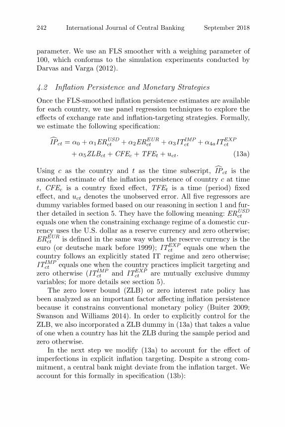
4.2 Inflation Persistence and Monetary Strategies

Once the FLS-smoothed inflation persistence estimates are availablefor each country, we use panel regression techniques to explore theeffects of exchange rate and inflation-targeting strategies. Formally,we estimate the following specification:

IPct = α0 + α1ERUSDct + α2EREUR

ct + α3ITIMPct + α4aITEXP

ct

+ α5ZLBct + CFEc + TFEt + uct. (13a)

Using c as the country and t as the time subscript, IPct is thesmoothed estimate of the inflation persistence of country c at timet, CFEc is a country fixed effect, TFEt is a time (period) fixedeffect, and uct denotes the unobserved error. All five regressors aredummy variables formed based on our reasoning in section 1 and fur-ther detailed in section 5. They have the following meaning: ERUSD

ct

equals one when the constraining exchange regime of a domestic cur-rency uses the U.S. dollar as a reserve currency and zero otherwise;EREUR

ct is defined in the same way when the reserve currency is theeuro (or deutsche mark before 1999); ITEXP

ct equals one when thecountry follows an explicitly stated IT regime and zero otherwise;ITIMP

ct equals one when the country practices implicit targeting andzero otherwise (ITIMP

ct and ITEXPct are mutually exclusive dummy

variables; for more details see section 5).The zero lower bound (ZLB) or zero interest rate policy has

been analyzed as an important factor affecting inflation persistencebecause it constrains conventional monetary policy (Buiter 2009;Swanson and Williams 2014). In order to explicitly control for theZLB, we also incorporated a ZLB dummy in (13a) that takes a valueof one when a country has hit the ZLB during the sample period andzero otherwise.

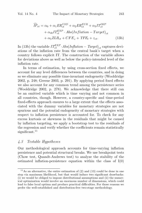
In the next step we modify (13a) to account for the effect ofimperfections in explicit inflation targeting. Despite a strong com-mitment, a central bank might deviate from the inflation target. Weaccount for this formally in specification (13b):


IPct = α0 + α1ERUSDct + α2EREUR

ct + α3ITIMPct

+ α4bITEXPct · Abs(Inflation − Target)ct

+ α5ZLBct + CFEc + TFEt + zct. (13b)

In (13b) the variable ITEXPct ·Abs(Inflation − Target)ct captures devi-

ations of the inflation rate from the central bank’s target when acountry follows explicit IT. The construction of the variable allowsfor deviations above as well as below the policy-intended level of theinflation rate.

In terms of estimation, by using cross-section fixed effects, weaccount for any level differences between the countries, and in doingso we eliminate any possible time-invariant endogeneity (Wooldridge2002, p. 248; Greene 2003, p. 291). By applying period fixed effectswe also account for any common trend among the persistence series(Wooldridge 2002, p. 278). We acknowledge that there still canbe an omitted variable which is time varying and not common inall countries, though. However, a country-specific and time-periodfixed-effects approach ensures to a large extent that the effects asso-ciated with the dummy variables for monetary strategies are notspurious and the potential endogeneity of monetary strategies withrespect to inflation persistence is accounted for. To check for anyexcess kurtosis or skewness in the residuals that might be causedby inflation targeting, we apply a bootstrap test to the residuals ofthe regression and verify whether the coefficients remain statisticallysignificant.11

4.3 Testable Hypotheses

Our methodological approach accounts for time-varying inflationpersistence and potential structural breaks. We use breakpoint tests(Chow test, Quandt-Andrews test) to analyze the stability of theestimated inflation-persistence equation within the class of I(0)

11As an alternative, the entire estimation of (2) and (13) could be done in onestep via maximum likelihood, but that would induce two significant drawbacks:(i) we would be obliged to impose distributional assumptions and (ii) the numer-ical optimization would involve an enormous number of dimensions, which couldlead to false local optima and produce practical difficulties. For those reasons weprefer the well-established and distribution-free two-stage methodology.


series. We assess a null hypothesis of no break at the 5 percentsignificance level and report the results in section 6.1.

Further, we assess the link between the exchange rate regimeand inflation persistence. Our working hypothesis is that there is nosuch link. We specify two possibilities of reserve currency in a con-straining exchange arrangement (U.S. dollar and euro, or deutschemark before 1999) and assess the coefficients α1 and α2 in specifi-cation (13). We formally test two null hypotheses, H0: α1 = 0 forUSD and H0: α2 = 0 for EUR, against the respective alternativehypotheses HA: α1 �= 0 and HA: α2 �= 0. If the null hypothesis isrejected, a negative (positive) coefficient indicates the existence of alink between the exchange rate regime and a decrease (increase) ininflation persistence. The results are reported in section 6.2.

Finally, we uncover the link between two degrees of inflation tar-geting and inflation persistence via an assessment of coefficients α3and α4 in specification (13). Here again we formally test two nullhypotheses depending on the type of IT strategy. Specifically, wetest H0: α3 = 0 for implicit IT and H0: α4 = 0 for explicit ITagainst their respective alternatives HA: α3 �= 0 and HA: α4 �= 0.Similarly as above, when the null hypothesis is rejected, a negative(positive) coefficient points to a decrease (increase) in inflation per-sistence with respect to the inflation-targeting strategy. The resultsare reported in section 6.3.

5. Data

Our sample covers sixty-eight countries that are listed in the appen-dix, table 3. The set contains both developed countries and emergingmarkets according to the Dow Jones list. We use quarterly inflationrates computed as changes in the consumer price index (CPI). CPIvalues were obtained from International Financial Statistics (IFS)of the International Monetary Fund (IMF) for two decades from1993:Q1 to 2013:Q4. In addition, the data were cross-checked oraugmented with the information provided by the statistical officesor central banks of the countries under research.

Further, in order to analyze the effect of monetary strategies, weform a data set indicating the date when implicit inflation targeting(IIT) and explicit inflation targeting (EIT) were adopted (table 3).Dummy variables for IIT or EIT take values of one when a country


exercises IIT or EIT and zero otherwise. Since both classifications aremutually exclusive, the estimated effects of both IT regimes are neteffects. The classification strategy follows Carare and Stone (2006)and is based on the information obtained from the individual centralbanks and numerous studies in the academic literature.12

In addition, we form a set of ZLB dummies that take a value ofone for those countries in our sample that have hit the ZLB duringthe sample period and zero otherwise. The ZLB is represented by a0.5 percent or lower value of a central policy rate that corresponds toempirically observed values associated with the ZLB-related mone-tary policy of major central banks in the United States, United King-dom, euro area, Canada, etc. (Buiter 2009; Swanson and Williams2014). Eleven countries plus the euro area in our sample that havehit a ZLB during the sample period are listed in the appendix, table3, with starting and ending dates when the central bank policy ratewas at or below 0.5 percent. If there is no ending date, the ZLB wasmaintained until the end of our sample period.

Further, we form the variable ITEXPct · Abs(Inflation − Target)ct

to capture absolute deviations of the inflation rate from the centralbank’s explicit inflation target. The changes in target levels overtime are accounted for. If a central bank has a target interval, weuse a midpoint as a reference value. In table 3 we provide informa-tion on countries’ inflation target rates as well as the timing of theiradoption.

Finally, we employ a de facto exchange rate regime classifica-tion of Reinhart and Rogoff (2004) that is available until 2001. Forthe later period (2002–13) a de facto regime classification is basedon their approach and checked against information obtained fromthe literature. We distinguish constraining exchange rate arrange-ments with respect to the U.S. dollar and the euro (or the deutsche

12Euro-area countries are primarily classified as explicitly targeting becauseof the declared commitment of the European Central Bank (ECB) to keep theannual inflation rate close to or below 2 percent. However, the classification ofindividual euro-area member states as explicit inflation targeters can certainlybe debated, as the ECB is not expected to stabilize inflation at close to 2 percentfor the individual member states but for the euro area as a whole. In this sensethe IMF classifies the monetary policy regime in euro-area member states as“other,” instead of “inflation targeting.” Therefore, as an alternative and robust-ness check we classify the euro-area member states as having floating exchangerates but without an inflation-targeting regime.


mark before 1999); on one occasion we also account for a peg to theBritish pound.13 The dummy variable for the exchange rate regimewith respect to a specific currency takes a value of one during peri-ods when such a regime was in power and zero otherwise (table 3).We account for a peg to a reserve currency along with constrainingintermediate regimes. In the case of a currency basket peg or itscrawling version, the dummy variables are coded to reflect a link tomore reserve currencies.

6. Empirical Results

6.1 Inflation Persistence Dynamics

First, we assess the stability of the estimated inflation-persistenceequation within the class of I(0) series by using two breakpoint tests:the Chow test and the Quandt-Andrews test (at the 5 percent sta-tistical significance level and under 10 percent trimming). For theChow test we assume the break point to be exogenous because thedate of IT adoption is known. Depending on the type of statisticsused (indicated in parentheses), the Chow test rejects the null ofno change in three (F -stat.), five (LR-stat.), and nine (Wald-type)cases out of thirty-one countries that adopted EIT during our sam-ple period. With the Quandt-Andrews test we tested for stabilitychanges at unknown break points to account for potential instabil-ities due to reasons other than IT adoption. The test rejects thenull of no change in six to thirty-nine cases, depending on the typeof statistics used.14 When comparing the results of both tests, we

13Euro-area countries are classified as floaters because, since its introduction,the euro freely floats. This is in line with the IMF exchange rate classification(AREAER) that classifies the euro-area member states as having freely floatingexchange rate regimes. During our sample period only Israel used the Britishpound as a reserve currency in its constraining exchange rate regime, when theBritish pound was part of a basket with the U.S. dollar.

14The Quandt-Andrews test provides maximum (MaxF), exponential average(ExpF), and average (AveF) test statistics with non-standard distributions. Thetrue distribution was developed by Andrews (1993) and the approximate asymp-totic p-values were provided by Hansen (1997). In our analysis, there are 3×2 = 6potential results (MaxF/ExpF/AveF × LR/Wald) on rejecting the null of nobreak. The specific numbers of rejections are twenty-nine, ten, four, thirty-nine,six, and twenty-five (observing the order of the test statistics list in parentheses).


conclude that instabilities in the persistence equation exist and anumber of them materialize for reasons additional to IT adoption.

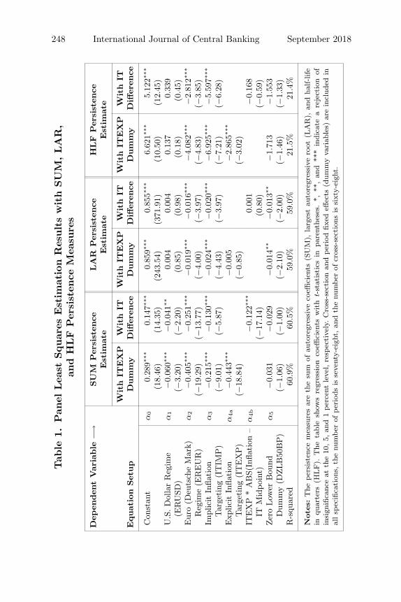
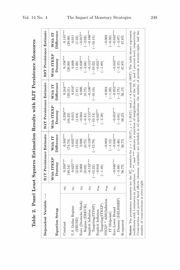
Second, we describe the essential facts related to the panel esti-mation.15 The key results are obtained based on the SUM persis-tence measure (table 1). Supplementary results are obtained basedon alternative measures: LAR (table 1), HLF (table 1), and RJT(table 2). Since all four IP measures are constructed differently, thepersistence estimates derived from the measures are not directlycomparable.

In our panel setup a constant is the same for all countries and rep-resents the average persistence of all countries under the conditionthat the exchange rate and IT regime-dependent dummies do notexhibit any effect. Based on the constant coefficient (α0) value, theaverage persistence is rather low. In our estimations we also accountfor country-specific and time fixed effects. The country-specific effectis basically an added constant for every given country, and its sumwith the global constant above (α0) represents the average coun-try persistence (again, under the condition that the exchange-rate-dependent and IT-regime-dependent dummies do not exhibit anyeffect). Based on the SUM measure, the values of country-specificeffects range from 0 to about |0.7|; this means that inflation per-sistence is strongly country dependent. Since we have sixty-eightcountries, the individual fixed-effect coefficients are not reported.

Time fixed effects account for a common trend in inflation per-sistence among countries. In figure 1 we present a plot of thoseestimated period fixed effects; they are obtained from the panel spec-ification (13a) estimated with the different IP measures defined in(3), (6), (7), and (9). Through period fixed effects we control forthe downward trend in the IP dynamics that changed into a gen-eral increase after 2001 and culminated with the financial crisis in2008. Later this pattern is characterized by a mild decline. Thesefeatures were well captured by period-specific effects, as advocatedin section 4.2.

Further, in figure 2, we present plots of the averages of theFLS-smoothed inflation persistence based on the SUM persistence

15The panel regression results largely stay the same when applying a boot-strap test to the residuals, as none of the estimated coefficients’ significance levelschange when looking at the bootstrap distribution.


Tab

le1.

Pan

elLea

stSquar

esEst

imat

ion

Res

ults

with

SU

M,LA

R,

and

HLF

Per

sist

ence

Mea

sure

s

Dep

enden

tV

aria

ble

−→SU

MPer

sist

ence

LA

RPer

sist

ence

HLF

Per

sist

ence

Est

imat

eEst

imat

eEst

imat

e

Wit

hIT

EX

PW

ith

ITW

ith

ITEX

PW

ith

ITW

ith

ITEX

PW

ith

ITEquat

ion

Set

up

Dum

my

Diff

eren

ceD

um

my

Diff

eren

ceD

um

my

Diff

eren

ce

Con

stan

tα

00.

289∗∗

∗0.

147∗∗

∗0.

859∗∗

∗0.

855∗∗

∗6.

621∗∗

∗5.

122∗∗

∗

(18.

46)

(14.

35)

(243

.54)

(371

.91)

(10.

50)

(12.

45)

U.S

.D

olla

rR

egim

eα

1−

0.06

0∗∗∗

−0.

041∗∗

0.00

40.

004

0.13

70.

339

(ER

USD

)(−

3.20

)(−

2.20

)(0

.85)

(0.9

8)(0

.18)

(0.4

5)E

uro

(Deu

tsch

eM

ark)

α2

−0.

405∗∗

∗−

0.25

1∗∗∗

−0.

019∗∗

∗−

0.01

6∗∗∗

−4.

082∗∗

∗−

2.81

2∗∗∗

Reg

ime

(ER

EU

R)

(−19

.29)

(−13

.77)

(−4.

00)

(−3.

97)

(−4.

83)

(−3.

85)

Impl

icit

Infla

tion

α3

−0.

215∗∗

∗−

0.13

0∗∗∗

−0.

024∗∗

∗−

0.02

0∗∗∗

−6.

925∗∗

∗−

5.59

7∗∗∗

Tar

geti

ng(I

TIM

P)

(−9.

01)

(−5.

87)

(−4.

43)

(−3.

97)

(−7.

21)

(−6.

28)

Exp

licit

Infla

tion

α4a

−0.

443∗∗

∗−

0.00

5−

2.86

5∗∗∗

Tar

geti

ng(I

TE

XP

)(−

18.8

4)(−

0.85

)(−

3.02

)IT

EX

P*

AB

S(In

flati

on–

α4b

−0.

122∗∗

∗0.

001

−0.

168

ITM

idpo

int)

(−17

.14)

(0.8

0)(−

0.59

)Zer

oLow

erB

ound

α5

−0.

031

−0.

029

−0.

014∗∗

−0.

013∗∗

−1.

713

−1.

553

Dum

my

(DZLB

50B

P)

(−1.

06)

(−1.

00)

(−2.

10)

(−2.

00)

(−1.

46)

(−1.

33)

R-s

quar

ed60

.9%

60.5

%59

.0%

59.0

%21

.5%

21.4

%

Note

s:T

heper

sist

ence

mea

sure

sar

eth

esu

mof

auto

regr

essi

veco

effici

ents

(SU

M),

larg

est

auto

regr

essi

vero

ot(L

AR

),an

dha

lf-life

inqu

arte

rs(H

LF).

The

tabl

esh

ows

regr

essi

onco

effici

ents

wit

ht-

stat

isti

csin

pare

nthe

ses.

*,**

,an

d**

*in

dica

tea

reje

ctio

nof

insi

gnifi

canc

eat

the

10,5,

and

1per

cent

leve

l,re

spec

tive

ly.C

ross

-sec

tion

and

per

iod

fixed

effec

ts(d

umm

yva

riab

les)

are

incl

uded

inal

lsp

ecifi

cati

ons,

the

num

ber

ofper

iods

isse

vent

y-ei

ght,

and

the

num

ber

ofcr

oss-

sect

ions

issi

xty-

eigh

t.


Tab

le2.

Pan

elLea

stSquar

esEst

imat

ion

Res

ults

with

RJT

Per

sist

ence

Mea

sure

s

Dep

enden

tV

aria

ble

−→R

1T

Per

sist

ence

Est

imat

eR

4T

Per

sist

ence

Est

imat

eR

8T

Per

sist

ence

Est

imat

e

Wit

hIT

EX

PW

ith

ITW

ith

ITEX

PW

ith

ITW

ith

ITEX

PW

ith

ITEquat

ion

Set

up

Dum

my

Diff

eren

ceD

um

my

Diff

eren

ceD

um

my

Diff

eren

ce

Con

stan

tα

00.

350∗

∗∗0.

344∗

∗∗0.

256∗

∗∗0.

244∗

∗∗0.

156∗

∗∗0.

145∗

∗∗

(49.

54)

(74.

74)

(34.

33)

(50.

31)

(20.

99)

(29.

99)

U.S

.D

olla

rR

egim

eα

10.

025∗

∗∗0.

025∗

∗∗0.

015

0.01

6∗0.

009

0.01

1(E

RU

SD)

(2.9

3)(3

.04)

(1.6

4)(1

.81)

(1.0

6)(1

.22)

Eur

o(D

euts

che

Mar

k)α

20.

000

0.00

6−

0.00

40.

006

−0.

026∗

∗∗−

0.01

7∗∗

Reg

ime

(ER

EU

R)

(0.0

3)(0

.75)

(−0.

41)

(0.7

5)(−

2.66

)(−

2.02

)Im

plic

itIn

flati

onα

3−

0.13

2∗∗∗

−0.

128∗

∗∗−

0.11

5∗∗∗

−0.

106∗

∗∗−

0.11

5∗∗∗

−0.

106∗

∗∗

Tar

geti

ng(I

TIM

P)

(−12

.22)

(−12

.79)

(−10

.14)

(−10

.10)

(−10

.22)

(−10

.15)

Exp

licit

Infla

tion

α4a

−0.

016

−0.

027∗

∗−

0.02

1∗

Tar

geti

ng(I

TE

XP

)(−

1.48

)(−

2.38

)(−

1.89

)IT

EX

P*

AB

S(In

flati

on–

α4b

−0.

004

−0.

004

−0.

002

ITM

idpoi

nt)

(−1.

12)

(−1.

29)

(−0.

50)

Zer

oLow

erB

ound

α5

−0.

046∗

∗∗−

0.04

5∗∗∗

−0.

053∗

∗∗−

0.05

2∗∗∗

−0.

043∗

∗∗−

0.04

2∗∗∗

Dum

my

(DZLB

50B

P)

(−3.

48)

(−3.

46)

(−3.

81)

(−3.

75)

(−3.

15)

(−3.

07)

R-s

quar

ed56

.7%

56.7

%56

.2%

56.1

%47

.8%

47.8

%

Note

s:T

he

per

sist

ence

mea

sure

sar

eth

eR

2 jt

stat

isti

csfo

rj

=1

(R1T

),j

=4

(R4T

),an

dj

=8

per

iods

(R8T

).T

he

table

show

sre

gres

sion

coeffi

cien

tsw

ith

t-st

atis

tics

inpar

enth

eses

.*,

**,an

d**

*in

dic

ate

are

ject

ion

ofin

sign

ifica

nce

atth

e10

,5,

and

1per

cent

leve

l,re

spec

tive

ly.

Cro

ss-s

ecti

onan

dper

iod

fixe

deff

ects

(dum

my

vari

able

s)ar

ein

cluded

inal

lsp

ecifi

cati

ons,

the

num

ber

ofper

iods

isse

vent

y-ei

ght,

and

the

num

ber

ofcr

oss-

sect

ions

issi

xty-

eigh

t.


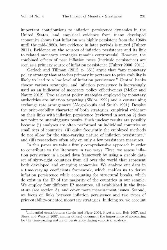
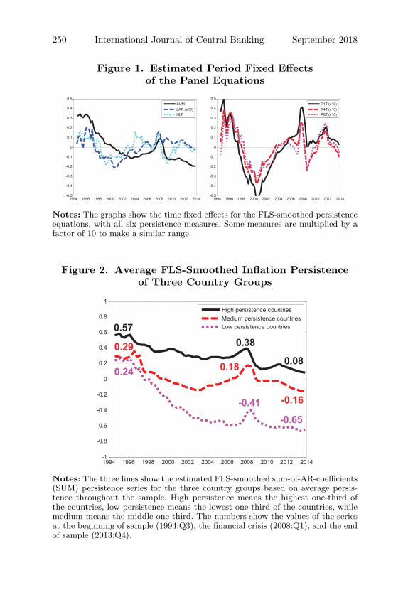
Figure 1. Estimated Period Fixed Effectsof the Panel Equations

Notes: The graphs show the time fixed effects for the FLS-smoothed persistenceequations, with all six persistence measures. Some measures are multiplied by afactor of 10 to make a similar range.

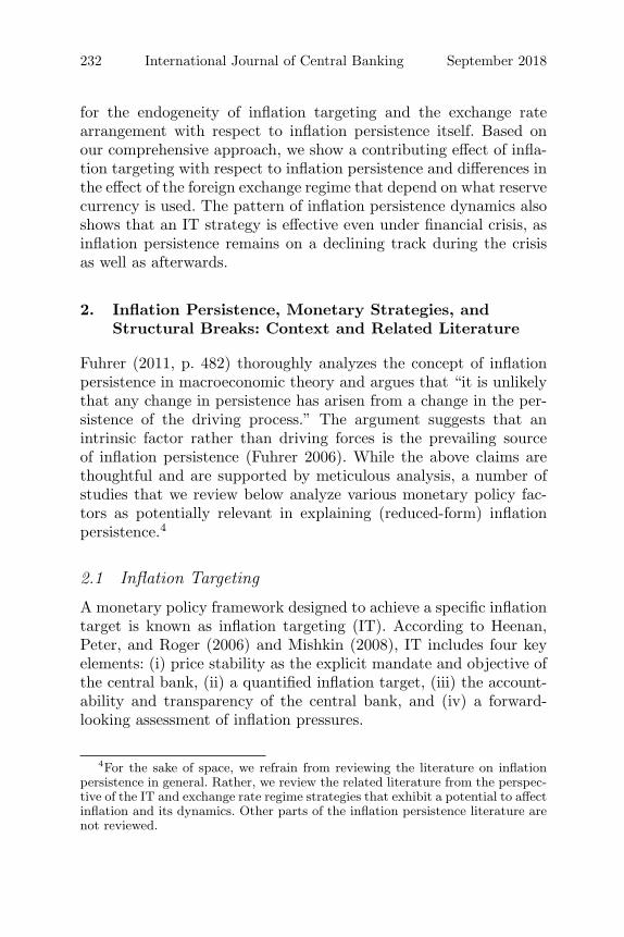
Figure 2. Average FLS-Smoothed Inflation Persistenceof Three Country Groups

Notes: The three lines show the estimated FLS-smoothed sum-of-AR-coefficients(SUM) persistence series for the three country groups based on average persis-tence throughout the sample. High persistence means the highest one-third ofthe countries, low persistence means the lowest one-third of the countries, whilemedium means the middle one-third. The numbers show the values of the seriesat the beginning of sample (1994:Q3), the financial crisis (2008:Q1), and the endof sample (2013:Q4).


measure for three country groups: low-, middle-, and high-persistence countries. The plots show (i) ample evidence of a com-mon pattern in inflation persistence among countries, albeit at dif-ferent IP levels, (ii) existence of structural breaks, and (iii) a uniformeffect of the financial crisis as IP was rising in all three groups dur-ing 2007–08.16 In addition, low-persistence countries even exhibitnegative inflation persistence. This finding could partly be a conse-quence of the time-varying steady-state level of the inflation rate,but it is not unusual, as it is reported in other studies as well (see,among others, Benati 2008; Meller and Nautz 2012; and Darvas andVarga 2014). This phenomenon can be explained with the help ofmicroeconomic price-setting models that often imply that “high per-sistence in the price level . . . translates into very low or even neg-ative persistence in inflation” (Cecchetti and Debelle 2006, p. 317).For example, in the canonical time-dependent price-setting model ofTaylor (1980), positive persistence in the price level implies negativeinflation persistence. Hence, price-level stickiness yields a plausibleinterpretation of the negative inflation persistence observed in somecountries in our sample. From a technical point of view it is alsoworth considering that state-space models, like the Kalman filteror FLS, compute the optimal increment of the state variable (inour example, the AR coefficients which are directly linked to per-sistence), holding the variance of this increment constant (or given,as in the FLS case). This can more easily lead to negative persis-tence values. The key takeaway from this is to look more at thedevelopment of IP than the exact levels of IP.

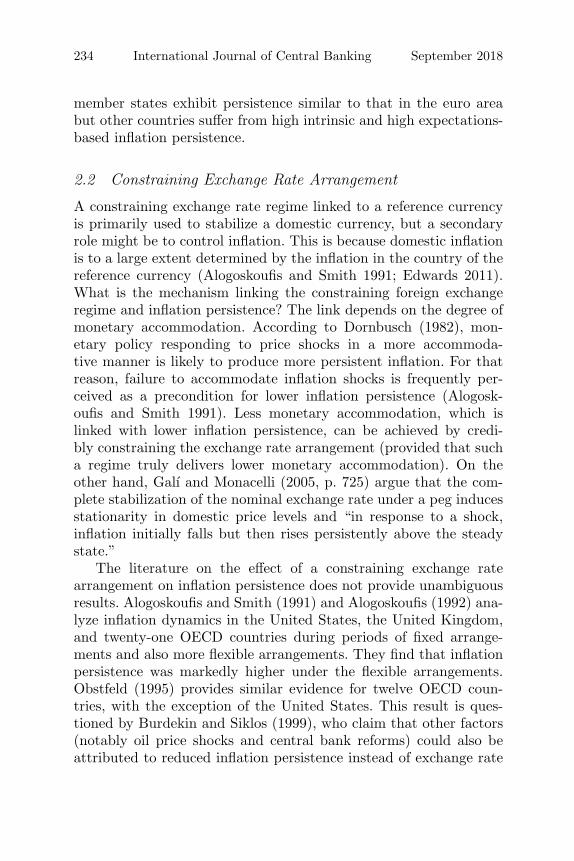
Finally, in figure 3 we present the persistence series for the UnitedStates and Germany (as a proxy for the euro area). The IP seriesis based on the estimated FLS-smoothed sum of AR coefficients(SUM). Their evolution is quite similar, as, in most cases, they seemto change direction at the same time, although the German series issmoother than the U.S. series.

16Principal components analysis (PCA) of the SUM-based IP series revealsthat the first two principal components explain 76 percent of the total variance(58 percent and 18 percent, respectively); the influence of the remaining compo-nents is negligible. The PCA result hints at the existence of a factor structure ininflation persistence across countries, possibly due to policy factors as argued byBenati and Surico (2008) and Cogley, Primiceri, and Sargent (2010).


Figure 3. FLS-Smoothed Inflation Persistence

Notes: The two lines show the estimated FLS-smoothed sum-of-AR-coefficients(SUM) persistence series for the United States and Germany. The beginning ofthe light gray background shows when the euro was adopted. The dark graybackground depicts when the United States adopted explicit inflation targeting.

6.2 Exchange Rate Regime and Inflation Persistence

The link between a constraining exchange arrangement and IP iscaptured by the coefficients α1 and α2, which represent the mar-ginal effects of dummy variables ERUSD and EREUR on inflationpersistence as an average for all countries. Relatively small and neg-ative values of the α1 coefficient based on the SUM measure (table 1)suggest that the USD-based constraining regime is mildly linked topersistence decrease. Results based on the LAR and HLF persistencemeasures are not available, as the estimate coefficients are statis-tically insignificant (table 1). Results based on the RJT measureproduce very small positive coefficients, but half of them are statis-tically insignificant (table 2). All of the results, taken together, indi-cate a limited but contributing link between the U.S.-dollar-basedconstraining exchange regime and inflation persistence.

Regimes using the euro (or deutsche mark) exhibit an order ofmagnitude larger effect that contributes to lower persistence sincethe SUM-based α2 coefficients are negative and relatively large


(table 1). Results obtained by using three other measures of infla-tion persistence are also negative and proportionally similar (tables 1and 2), given the differences in measure construction. Low Germaninflation and reasonably low inflation pursued by the ECB underthe Maastricht stability criterion along with the prudent monetarypolicies of both institutions have led to low or moderate inflationpersistence (Altissimo, Ehrmann, and Smets 2006; Meller and Nautz2012), as documented for much of the span of our sample. Based onsuch IP dynamics, the negative α2 coefficients come as a sensibleoutcome and the estimates provide consistent findings: the effect ofconstraining exchange regimes using the euro (or deutsche mark)is relatively strong and uniformly points at a link to a decrease ininflation persistence. The effect is also in accord with the dramaticdecrease in inflation persistence following the euro introduction thatis documented by Lopez and Papell (2012), and progressive inflationconvergence documented by Broz and Kocenda (2018).

The above results indicate some difference between the effects ofexchange rate regimes using different reserve currencies. Such dissim-ilarity materialized despite the strong constraints on domestic policyactions imposed by a commitment to a constraining exchange rateregime and limitations on how the monetary authorities can react tothe persistence of inflation shocks (Bleaney 2000). As a complement,in figure 3 we provide a plot of inflation persistence for the UnitedStates and Germany. Inflation persistence in the United States wasrelatively high for the initial two-thirds of the period under researchand, in fact, was rising prior to the financial crisis. Then it experi-enced a marked decline during 2006–08. This pattern is quite differ-ent from the global picture (figure 2), where a major increase in IPcoincides with the crisis period in 2008. The sharpest decline in U.S.inflation persistence occurs from mid-2007 and correlates with thesequence of cuts to the federal funds rate initiated in August 2007.An increase in the post-crisis IP is soon transformed into a subse-quent decline that coincides with the adoption of explicit inflationtargeting by the Federal Reserve in 2012. The German IP exhibits adifferent pattern: it is low for most of the period and declines in a sta-ble manner. A notable difference between U.S. and German inflationpersistence is visible with respect to the 2008 crisis, though. Duringthe crisis, German IP rises, albeit marginally, then declines and lev-els off. On the other hand, after the crisis U.S. inflation persistence


has been remarkably low. The difference between the patterns in theU.S. and German IP likely stems from the fact that post-crisis ECBinterest rate cuts were less pronounced than those of the FederalReserve.

Despite some differences in the effects, the results can be reason-ably explained. Bleaney (2000, p. 393) develops a model of inflationpersistence under a constraining exchange rate regime and arguesthat a “more constraining exchange rate regime tends to reducethe variance of inflation persistence across countries, because allcountries take on the inflation persistence of the reserve currencyin proportion to the degree of exchange rate constraint.” However,inflation persistence is not necessarily lower in a more constrainingarrangement. According to his model, the coincidence of low infla-tion persistence under a more constraining regime would emerge “ifthe exchange rate regime constrains the reserve currency to havelow inflation persistence, or if it happened to have low inflationpersistence by chance.” The above arguments imply that undera constraining exchange rate regime—linked to a specific reservecurrency—lower inflation persistence can be potentially importedunder the condition that in the reserve-currency country persistenceis low and its dynamics is stable. Pivetta and Reis (2007) provideevidence of high U.S. inflation from the end of World War II to thelate 1990s. Beechey and Osterholm (2012) argue that U.S. inflationpersistence decreased during recent decades (partly thanks to theFederal Reserve accentuating price stability in its monetary policy).This claim resonates well with our evidence on high U.S. persis-tence before the crisis and particularly low IP afterwards (figure 3).The above theoretical arguments along with the empirical evidencehelp to explain that a constraining exchange arrangement with theU.S. dollar as a reserve currency might suppress inflation persistencesomewhat less than one based on the euro (deutsche mark).

The above findings and interpretation are further complementedby testing the exchange rate channel of IP. We proceed by includingthe IP of Germany and the United States separately in the regres-sion ((13a); not shown formally) and at the same time we removethe IP of each country from a panel of dependent variables. Statisti-cally significant results are limited to the SUM measure and positivecoefficients amount to 0.4 for U.S. IP and 2.6 for German IP (detailsnot reported, available upon request). These marginal effects from


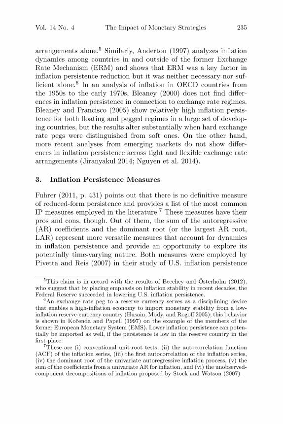
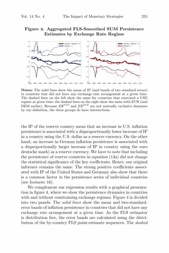
Figure 4. Aggregated FLS-Smoothed SUM PersistenceEstimates by Exchange Rate Regime

Notes: The solid lines show the mean of IP (and bands of two standard errors)in countries that did not have any exchange rate arrangement at a given time.The dashed lines on the left show the same for countries that exercised a USDregime at given time; the dashed lines on the right show the same with EUR (andDEM earlier). Because ERUSD and EREUR are not mutually exclusive dummiesby our definition, the three groups do have intersections.

the IP of the reserve country mean that an increase in U.S. inflationpersistence is associated with a disproportionally lower increase of IPin a country using the U.S. dollar as a reserve currency. On the otherhand, an increase in German inflation persistence is associated witha disproportionally larger increase of IP in country using the eurodeutsche mark) as a reserve currency. We have to note that includingthe persistence of reserve countries in equation (13a) did not changethe statistical significance of the key coefficients. Hence, our originalinference remains the same. The strong positive coefficients associ-ated with IP of the United States and Germany also show that thereis a common factor in the persistence series of individual countries(see footnote 16).

We complement our regression results with a graphical presenta-tion in figure 4, where we show the persistence dynamics in countrieswith and without constraining exchange regimes. Figure 4 is dividedinto two panels. The solid lines show the mean and two-standard-error bands of inflation persistence in countries that did not have anyexchange rate arrangement at a given time. As the FLS estimatoris distribution free, the error bands are calculated using the distri-bution of the by-country FLS point-estimate sequences. The dashed


lines in both left and right panels show the same information forcountries that exercised dollar-based or euro-based/deutsche-mark-based arrangements at a given time. The persistence in countriesusing a dollar-based regime was decreasing until 2002 and increasedafterwards, reaching the highest value during the 2008 crisis (figure4, left panel). Increasing persistence before the world financial cri-sis signals worsening monetary conditions in countries with tightexchange arrangements potentially transferred via the USD. A tem-poral drop in persistence after 2008 was quickly replaced by anincrease of persistence to a new level, slightly higher than prior to thecrisis. Inflation persistence in countries with floating exchange rateswas mostly somewhat lower than that of those with dollar-basedregimes and exhibits a more stable decreasing pattern. Persistencein countries using the euro (deutsche mark) as a reserve currencyexperienced a continuous decrease until 2000 and, after stabiliza-tion, began to marginally rise during the 2005–08 period (figure 4,right panel). After the financial crisis, inflation persistence began todecrease. In general, IP was also slightly lower and exhibited a morestable pattern than persistence in floating countries. The dynamicsof persistence in both panels indirectly supports our quantitativeresults presented in table 2 about the contribution a constrainingexchange rate regime makes in pacifying inflation persistence.

6.3 Inflation Targeting and Inflation Persistence

Coefficients α3 and α4a exhibit the marginal effects of two forms ofIT on inflation persistence. The negative values of the coefficients intables 1 and 2 represent consistent outcomes, indicating a decreasein inflation persistence. The coefficients (table 1; SUM) associatedwith explicit IT (α4a) are almost two times as large as the coeffi-cients of implicit IT (α3). This is quite a strong result, as our samplecontains sixty-eight countries, out of which forty-two have practicedsome type of IT during the time span. First, it shows that inflationtargeting contributes to lower inflation persistence. Second, it showsthat even its less strict version (IIT) possesses the power to tamepersistence.

The results based on the LAR persistence measure also show acontributing effect to lower inflation persistence (table 1), but theestimate for the EIT is statistically insignificant. The values of the


coefficients associated with the HLF measure indicate that implicitIT is more contributive than explicit IT (table 1). This finding mightstem from differences in the construction of the persistence measures.Recall that the HLF measure represents the number of periods afterwhich the absolute value of the impulse response is indefinitely below0.5. Since inflation is usually higher under implicit IT than underexplicit IT, it is more likely that the impulse response of the individ-ual IP will be above the 0.5 threshold longer under implicit IT. Inthis sense, implicit IT provides more room for potential improvementof the HLF measure as the coefficient values attest.

Further, the results based on RJT measures (table 2) also showthat the effect of implicit IT on inflation persistence seems to belarger than that of explicit IT. However, the coefficients show thatthe effect of explicit IT is rather stable but that of implicit IT dimin-ishes with the time over which the specific RJT measure is computed.Thus, after all, results from the SUM measure (table 1) and thosebased on the HLF (table 1) and RJT measures (table 2) provide aqualitatively similar inference.

Our results also contribute to the debate on how the zero lowerbound (ZLB) has affected inflation persistence due to the constraintit imposes on conventional monetary policy (Buiter 2009; Swansonand Williams 2014). The coefficients of the ZLB dummy (α5) are rel-atively small, negative, and statistically significant when measuredby the LAR (table 1) and RJT (table 2) measures; they are alsonegative but statistically insignificant in the case of the SUM andHLF measures (table 1). The negative marginal effect of the ZLBmeans that, ceteris paribus, once a country hits the ZLB its infla-tion persistence mildly decreases. This result should not be taken asadvice to lower the interest rate to achieve lower IP, though. Underthe ZLB, inflation is low anyway. Plus, the limited fraction of ourresearch time span, during which some countries entered the ZLB,suggests that we take the ZLB effect with a grain of salt.

Further, we show how deviations of the inflation rate fromthe central bank’s explicit inflation target affect inflation persis-tence. The results are limited to the SUM measure (table 1) deliv-ering a statistically significant coefficient (α4b) associated withthe deviation-from-the-target variable (ITEXP

ct · Abs(Inflation −Target)ct); other measures produce statistically insignificant coef-ficients. A negative coefficient (α4b) means that, ceteris paribus,


there exists a pull to return to the inflation persistence mean asa central bank moves from its inflation target. However, the extentof this impact should not be overstated: when inflation is 1 percentfrom its target, the average marginal effect of the pull causes lowerpersistence of about 0.1 percent.17

Finally, in figure 5 we bring forth a graphical presentation ofthe persistence dynamics. The solid lines show the mean and two-standard-error bands of inflation persistence in countries that didnot practice any form of IT. The dashed lines in the left panel showthe same information for countries that implicitly (and only implic-itly) exercised inflation targeting at any given time. The dashed linesin the right panel show the inflation persistence in countries withexplicit inflation targeting. Inflation persistence in countries practic-ing any form of IT shows a very stable pattern of gradual decline thatis not interrupted even by the 2008 financial crisis. The key differencebetween the two panels is the dramatically larger decrease in per-sistence for countries with implicit IT. After 2002, the paths of thepersistence of implicitly IT and non-IT countries even diverge. Dur-ing most of the period under research, the persistence in explicitly

17As a complementary check we performed a formal test for the statistical sig-nificance of the difference between explicit and implicit inflation targeters. For allIP measures, the effects of the EIT and IIT were found to be statistically differentat the 1 percent significance level (not reported but available upon request).

Further, since the ECB is not expected to stabilize inflation at close to 2percent for the individual member states but for the euro area as a whole, weperformed a robustness check. We ran our panel regressions again under an alter-native classification of the euro-area member states: floating exchange rates butwithout an inflation-targeting regime. In terms of the signs and statistical signif-icance of the coefficients, the results did not materially change (not reported butavailable upon request). The single notable change was a statistical significancegain (under the alternative classification) of the coefficient capturing absolutedeviations of the inflation rate from the central bank’s explicit inflation target(α4b) when using the RJT measure (lag 1 and 4). Hence, the results reportedin tables 1 and 2 are robust with respect to the alternative classification of theeuro-area member states.

Finally, one has to note that the number of countries practicing any form ofIT has been growing. Consequently, from our IP estimates we witness a mostlydecreasing pattern of IP over time (figure 5). These two phenomena might pro-duce an inverse relationship. In order to rule out the possibility of such a spuriouslink, we repeated the estimation with the difference of IP as our explanatory vari-able in (13). This robustness check produced negative and statistically significantcoefficients (α3 and α4; not reported, available upon request) and confirmed thecontributive effect of IT on inflation persistence.


Figure 5. Aggregated FLS-Smoothed SUM PersistenceEstimates by Inflation Targeting

Notes: The solid lines show the mean of IP (and bands of two standard errors)in countries that did not have inflation targeting at a given time. The dashedlines on the left show the same for countries that implicitly (and only implicitly)exercised inflation targeting at a given time; the dashed lines on the right showthe same with explicit inflation targeting. Because ITIMP and ITEXP are mutuallyexclusive dummies by our definition, the three groups are disjunctive and theirunion gives all the countries at every time point.

targeting countries is low and stable, and exhibits a mild decreasingpattern that is interrupted only by temporary and marginal increasesaround 2000 and in 2008. Further, confidence bands around the per-sistence of the explicit-IT countries are visibly narrower that thoserelated to the persistence of non-IT countries. The IP pattern incountries without IT is quite different. A gradual decline during the1990s is replaced in 2002 by an upward trend and IP sharply risesprior to and during the 2008 financial crisis. A post-crisis drop isthen replaced by an increase in IP to a new level that is higher thanthe low IP in 2002. In general, persistence dynamics is in line withour quantitative results and supports the favorable effect of IT withrespect to inflation persistence, even during the financial crisis.

7. Conclusions

We provide a comprehensive analysis of the link between price-stability-oriented monetary strategies and inflation persistence. Weanalyze the dynamics of inflation persistence in a panel of sixty-eightcountries by employing quarterly inflation rates for the period from


1993:Q1 to 2013:Q4. The panel data set contains both developedcountries and emerging markets. This exceptionally wide coverageenables us to provide a truly “big picture” of the analyzed phe-nomenon. In our analysis we first use the time-varying coefficientsapproach to derive four different measures of inflation persistencefor each individual country. The time-varying persistence approachhelps us to account for structural breaks in persistence that in factexist in a majority of the countries in our sample. In the secondstage, we estimate links between inflation persistence and two policystrategies that possess potential to affect inflation persistence. Thestrategies are inflation targeting and a constraining exchange ratearrangement. We distinguish between implicit and explicit inflation-targeting strategies of central banks, and also identify constrainingexchange rate arrangements with respect to the U.S. dollar and euro(or deutsche mark).

Based on our results, we show a contributing effect of inflationtargeting with respect to inflation persistence. The effect of explicitIT is stronger than that of implicit targeting. However, even the lessstrict version (IIT) possesses the power to tame persistence. Thelink between inflation persistence and constraining exchange rateregimes is, in general, less pronounced than that of IT and the effectis statistically significant across all IP measures. Our results alsocontribute to the debate on how the zero lower bound has affectedinflation persistence due to the constraint that it imposes on conven-tional monetary policy. We show that once a country hits the ZLB,its inflation persistence mildly decreases. Finally, we assess how devi-ations of the inflation rate from the central bank’s explicit inflationtarget impact inflation persistence. We show that there exists a mildpull to return to the inflation persistence mean once a central bankmoves away from its inflation target.

Further, regimes with the U.S. dollar as a reserve currencyseem to be less effective in taming inflation persistence than thoseusing the euro (deutsche mark). On the other hand, U.S. infla-tion persistence exhibits a disproportionally lower effect on othercountries’ persistence than its German counterpart. Our evidenceshows that the effect of the exchange rate regime on inflation per-sistence depends on the reserve currency and correlates with thecharacteristics of inflation persistence in the country of the reservecurrency.


Our findings show that price-stability-oriented policy strategiesseem to possess the ability to help reduce inflation persistence. Inthis respect, both monetary strategies provide central banks with anenlarged “policy space” to deal with temporary price shocks, albeitto different extents. This result is in line with the argument voiced bySiklos (2017, p. 42) that “low and stable inflation continues to rep-resent an essential ingredient of good practice in monetary policy.”We conclude that IT seems to be an effective monetary strategy, asinflation persistence in countries practicing any form of IT exhibitsa stable pattern of gradual decline, which is not interrupted even bythe 2008 financial crisis.


Appen

dix

Tab

le3.

Tim

ings

ofIn

flat

ion

Tar

geting,

Exch

ange

Rat

e,an

dZer

oLow

erB

ound

Reg

imes

ZLB

Sta

rtN

o.C

ountr

yII

TSta

rtEIT

Sta

rtIT

Val

ue

(End)

ER

Inte

rval

sER

Types

1A

rgen

tina

1964

–197

1U

SD19

85–1

986

USD

1991

:Q2–

2002

:Q3

USD

2A

ustr

alia

Jan.

1990

Apr

.19

932.

50±

0.50

1972

–198

7U

SD3

Aus

tria

Jan.

1999

1.75

±0.

25M

ay20

1319

54–1

959

USD

1960

–199

8D

EM

4B

angl

ades

hJu

l.20

13(1

972)

–198

2G

BP

1983

–200

2U

SD5

Bel

gium

Jan.

1999

1.75

±0.

25M

ay20

1319

54–1

955

USD

1956

–199

8D

EM

6B

razi

lJu

n.19

994.

50±

2.00

(194

5)–1

950

USD

1967

–199

8U

SD7

Bul

gari

aJa

n.20

10(1

945)

–198

9U

SD19

97–

DE

M/E

UR

8C

anad

aM

ar.19

912.

00±

1.00

Mar

.20

09(1

945)

–195

0U

SD(J

ul.20

10)

1963

–196

9U

SD9

Chi

leSe

p.19

90Se

p.19

994.

00±

0.00

1960

–196

2U

SDJa

n.20

013.

00±

1.00

1973

:Q2–

1999

:Q3

USD

1982

–198

3D

EM

10C

hina

Jan.

2003

1994

–U

SD11

Col

ombi

aJa

n.19

91Se

p.19

993.

00±

1.00

(194

5)–1

983

USD

1985

–199

8U

SD12

Cze

chR

epub

licD

ec.19

972.

00±

1.00

Jul.

2012

(199

1)–1

997:

Q2

USD

(199

1)–1

997:

Q2

DE

M

(con

tinu

ed)

Vol. 14 No. 4 The Impact of Monetary Strategies 263Tab

le3.

(Con

tinued

)

ZLB

Sta

rtN

o.C

ountr

yII

TSta

rtEIT

Sta

rtIT

Val

ue

(End)

ER

Inte

rval

sER

Types

13D

enm

ark

Jun.

2012

(194

5)–1

951

USD

1952

–D

EM

/EU

R14

Egy

pt(1

945)

–195

0G

BP

1963

–200

2U

SD15

Est

onia

Jan.

2011

1.75

±0.

25M

ay20

1319

92–2

010

DE

M/E

UR

16Fin

land

Feb.

1993

2.00

±0.

00M

ay20

1319

49–1

972

USD

Jan.

1999

1.75

±0.

0019

73–1

998

DE

M17

Fran

ceJa

n.19

991.

75±

0.25

May

2013

1949

–197

1U

SD19

72–1

998

DE

M18

Ger

man

yJa

n.19

75Ja

n.19

991.

75±

0.25

May

2013

(194

5)–1

970

USD

1971

(DE

M)

1972

USD

1973

–199

8(D

EM

)19

Gre

ece

Jan.

2001

1.75

±0.

25M

ay20

1319

50–1

981

USD

1985

–200

0D

EM

/EU

R20

Hon

gK

ong

Dec

.20

08(1

945)

–197

2U

SD19

83:Q

4–U

SD21

Hun

gary

Jun.

2001

3.00

±0.

00(1

946:

Q3)

–200

1:Q

1D

EM

/EU

R22

Icel

and

Mar

.20

012.

50±

0.00

1947

–197

7U

SD19

84–2

000

DE

M/E

UR

23In

dia

(194

5)–1

969

GB

P19

70U

SD19

71–1

978

GB

P19

80–2

007

USD

(con

tinu

ed)

264 International Journal of Central Banking September 2018Tab

le3.

(Con

tinued

) ZLB

Sta

rtN

o.C

ountr

yII

TSta

rtEIT

Sta

rtIT

Val

ue

(End)

ER

Inte

rval

sER

Types

24In

done

sia

May

1999

Jul.

2005

5.00

±1.

00(1

945)

–194

9G

BP

1969

–199

7U

SD25

Iran

1954

–197

6U

SD26

Irel

and

Jan.

1999

1.75

±0.

25M

ay20

1319

80–1

998

DE

M27

Isra

elJu

n.19

92Ju

n.19

978.

50±

1.50

(194

8)–1

950

GB

PJa

n.19

994.

00±

0.00

1962

–197

0G

BP

Jan.

2000

3.50

±0.

5019

71–1

975

USD

Jan.

2001

3.00

±0.

5019

80–1

998

GB

PJa

n.20

022.

50±

0.50

1986

–199

8U

SDJa

n.20

032.

00±

1.00

28It

aly

Jan.

1999

1.75

±0.

25M

ay20

1319

52–1

975

USD

1979

:Q2–

1998

DE

M29

Japa

nJa

n.20

10Fe

b.20

121.

00±

1.00

Oct

.19

9519

49–1

977

USD

Jan.

2013

2.00

±0.

0030

Jord

an(1

945)

–197

1G

BP

1972

–U

SD19

75–1

988

SDR

31K

orea

(Sou

th)

Apr

.19

98Ja

n.20

002.

50±

1.00

(194

5)–1

997

USD

Jan.

2001

3.00

±1.

00Ja

n.20

043.

00±

0.50

Jan.

2010

3.00

±1.

00Ja

n.20

133.

00±

0.50

Jan.

2016

2.00

±0.

00

(con

tinu

ed)


le3.

(Con

tinued

)

ZLB

Sta

rtN

o.C

ountr

yII

TSta

rtEIT

Sta

rtIT

Val

ue

(End)

ER

Inte

rval

sER

Types

32K

uwai

t(1

959)

–196

1D

EM

1969

–U

SD19

75:Q

2–20

02D

EM

/EU

R20

07:Q

3–E

UR

33Lat

via

1995

–201

3D

EM

/EU

R34

Lit

huan

ia19

95–2

001

USD

2002

–201

4E

UR

35Lux

embo

urg

Jan.

1999

1.75

±0.

25M

ay20

13(1

945)

–195

5U

SD19

56–1

998

DE

M36

Mal

aysi

a19

46–1

975

GB

P19

76–1

997

USD

1999

–200

5U

SD37

Mau

riti

us(1

945)

–197

5D

EM

1972

:Q3

USD

1976

–199

4:Q

2U

SD38

Mex

ico

Jan.

1996

Jan.

2001

3.00

±1.

00(1

945)

–197

6:Q

3U

SD19

82:Q

3–19

94U

SD39

Mor

occo

(194

5)–

DE

M40

Net

herl

ands

Jan.

1999

1.75

±0.

25M

ay20

1319

51–1

970

USD

1971

–199

8D

EM

41N

ewZea

land

Mar

.19

902.

00±

1.00

(194

5)–1

971

GB

P19

72–1

982

USD

Peg

via

AU

D

(con

tinu

ed)

266 International Journal of Central Banking September 2018Tab

le3.

(Con

tinued

)

ZLB

Sta

rtN

o.C

ountr

yII

TSta

rtEIT

Sta

rtIT

Val

ue

(End)

ER

Inte

rval

sER

Types

42N

iger

ia(1

945)

–197

1D

EM

1983

:Q3–

1984

:Q2

USD

1991

:Q3–

1998

USD

43N

orw

ayFe

b.19

99M

ar.20

012.

50±

0.00

(194

5)–1

972

USD

1973

–199

2D

EM

44Pak

ista

n(1

945)

–197

1G

BP

1972

–200

7U

SD45

Per

uJa

n.20

022.

00±

1.00

(194

5)–1

971

USD

1994

–200

7U

SD46

Phi

lippi

nes

Jul.

1993

Jan.

2002

4.00

±1.

0019

52–1

956

USD

1962

–196

8U

SD19

73–1

982

USD

1986

–199

0U

SD47

Pol

and

Aug

.19

97O

ct.19

982.

50±

1.00

1990

–200

0U

SD19

91–2

000

DE

M/E

UR

48Por

tuga

lJa

n.19

991.

75±

0.25

May

2013

(194

5)–1

972

USD

1973

–199

8D

EM

49R

oman

iaJa

n.20

02A

ug.20

053.

00±

1.00

1990

–200

2U

SD19

90–1

993

DE

M20

09–

EU

R50

Rus

sia

Jan.

2001

1995

–199

8U

SD20

05–2

008

USD

2005

–200

8D

EM

/EU

R

(con

tinu

ed)


le3.

(Con

tinued

) ZLB

Sta

rtN

o.C

ountr

yII

TSta

rtEIT

Sta

rtIT

Val

ue

(End)

ER

Inte

rval

sER

Types

51Sa

udiA

rabi

a(1

945)

–195

8D

EM

1959

–U

SD52

Sing

apor

eJa

n.20

09(1

945)

–197

1D

EM

1972

–199

8U

SD53

Slov

akR

epub

licJa

n.20

091.

75±

0.25

May

2013

(199

1)–1

997

USD

(199

1)–1

997

DE

M19

99–2

008

EU

R54

Slov

enia

Nov

.20

03Ja

n.20

071.

75±

0.25

May

2013

1993

–200

6D

EM

/EU

R55

Sout

hA

fric

aJa

n.19

90Fe

b.20

004.

50±

1.50

(194

5)–1

973

DE

M56

Spai

nJa

n.19

95Ja

n.19

991.

75±

0.25

May

2013

(194

5)–1

946

USD

1949

–198

0U

SD19

81–1

998

DE

M57

SriLan

ka(1

945)

–196

7D

EM

1972

–201

1U

SD58

Suda

n19

58–1

978

USD

(199

0)–

USD

59Sw

eden

Jan.

1993

2.00

±1.

00A

pr.20

0919

46–1

972

USD

(Aug

.20

10)

1973

–199

2D

EM

60Sw

itze

rlan

dJa

n.19

75Ja

n.20

001.

00±

1.00

Dec

.20

08(1

945)

–197

3U

SD19

82–

DE

M/E

UR

61Tai

wan

——

62T

haila

ndM

ay20

001.

75±

1.75

(194

5)–1

947

DE

MSe

p.20

091.

75±

1.25

1948

–199

7U

SDJa

n.20

152.

50±

1.50

(con

tinu

ed)


Tab

le3.

(Con

tinued

)

ZLB

Sta

rtN

o.C

ountr

yII

TSta

rtEIT

Sta

rtIT

Val

ue

(End)

ER

Inte

rval

sER

Types

63Tun

isia

(194

5)–

DE

M64

Tur

key

Jan.

2002

Jan.

2006

5.50

±0.

0019

46–1

953

USD

1961

–198

0U

SD19

98–2

000

DE

M/E

UR

65U

krai

ne19

97–2

006

USD

66U

nite

dK

ingd

omO

ct.19

932.

00±

0.00

Mar

.20

09(1

945)

–197

1U

SD19

91–1

992

DE

M67

Uni

ted

Stat

es19

92Ja

n.20

122.

00±

0.00

Jan.

2009

(194

5)–

(USD

)68

Ven

ezue

la(1

945)

–198

2U

SD19

94–

USD

Note

s:Im

plic

it(I

IT)

and

expl

icit

(EIT

)in

flati

onta

rget

ing

and

zero

low

erbou

nd(Z

LB

)re

gim

esha

vem

ostl

yst

arti

ngda

tes

(no

ITre

gim

eha

sen

ded

yet,

and

only

two

ZLB

regi

mes

have

ende

dw

ithi

nou

rsa

mpl

eti

me

span

).W

ere

por

tth

ese

wit

hm

onth

lypr

ecis

ion.

Ann

ual

infla

tion

targ

etva

lues

orba

nds

are

alw

ays

conv

erte

dto

am

idpoi

ntpl

us/m

inus

aha

lfra

nge

(zer

oin

case

ofex

act

targ

etra

te),

and

are

repor

ted

inper

cent

age

poi

nts;

the

conv

ersi

onw

asdo

nefo

rco

nven

ienc

eof

esti

mat

ion

irre

spec

tive

ofw

heth

era

cent

ral

bank

has

asp

ecifi

cra

teor

band

asa

targ

et.

For

the

euro

zone

we

use

valu

esof

1.75

±0.

25;

this

solu

tion

refle

cts

asl

ight

lyva

gue

com

mit

men

tof

the

Eur

opea

nC

entr

alB

ank

(EC

B)

toke

epth

ean

nual

infla

tion

rate

clos

eto

orbel

ow2

per

cent

(diff

eren

tta

rget

valu

eop

tion

sre

flect

ing

the

com

mit

men

tdo

not

yiel

dm

ater

ially

differ

ent

resu

lts)

.Fo

rso

me

ITva

lues

(EIT

and

ZLB

star

ting

date

s)a

shad

edba

ckgr

ound

mar

ksth

atth

esp

ecifi

cco

untr

yad

opte

da

give

nre

gim

ebec

ause

ofit

seu

ro-a

rea

mem

ber

ship

.T

heex

chan

gera

tere

gim

e(E

R)

inte

rval

sar

ere

por

ted

wit

hqu

arte

rly

prec

isio

n.T

heQ

1no

tati

ons

atst

arti

ngda

tes

and

Q4

nota

tion

sat

endi

ngda

tes

are

omit

ted.

The

star

ting

date

sin

pare

nthe

ses

indi

cate

the

appr

oxim

ate

star

ting

poi

ntof

agi

ven

ER

regi

me,

but

this

does

not

affec

tou

ran

alys

is,as

our

data

sam

ple

star

tsla

ter

on.In

case

ofa

vari

ant

ofcu

rren

cyba

sket

peg

s,th

eex

chan

gera

tere

gim

ein

volv

esa

peg

tom

ore

than

one

curr

ency

duri

ngth

esp

ecifi

cper

iod.


References

Alogoskoufis, G. S. 1992. “Monetary Accommodation, ExchangeRate Regimes and Inflation Persistence.” Economic Journal 102(412): 461–80.

Alogoskoufis, G. S., and R. P. Smith. 1991. “The Phillips Curve, thePersistence of Inflation, and the Lucas Critique: Evidence fromExchange Rate Regimes.” American Economic Review 81 (6):1254–75.

Altissimo, F., M. Ehrmann, and F. Smets. 2006. “Inflation Persis-tence and Price-Setting Behaviour in the Euro Area: A Summaryof the IPN Evidence.” ECB Occasional Paper No. 46.

Anderton, R. 1997. “Did the Underlying Behaviour of Infla-tion Change in the 1980s? A Study of 17 Countries.”Weltwirtschaftliches Archiv 133 (1): 22–38.

Andrews, D. 1993. “Tests for Parameter Instability and StructuralChange with Unknown Change Point.” Econometrica 61 (4):821–56.

Ascari, G., and T. Ropele. 2012. “Sacrifice Ratio in a Medium-ScaleNew Keynesian Model.” Journal of Money, Credit and Banking44 (2–3): 457–67.

Ascari, G., and A. M. Sbordone. 2014. “The Macroeconomicsof Trend Inflation.” Journal of Economic Literature 52 (3):679–739.

Banerjee, A., R. Lumsdaine, and J. Stock. 1992. “Recursive andSequential Tests of the Unit-Root and Trend-Break Hypotheses:Theory and International Evidence.” Journal of Business andEconomic Statistics 10 (3): 271–88.

Baxa, J., R. Horvath, and B. Vasıcek. 2014. “How Does Mone-tary Policy Change? Evidence on Inflation-Targeting Countries.”Macroeconomic Dynamics 18 (3): 593–630.

Beechey, M., and P. Osterholm. 2012. “The Rise and Fall of U.S.Inflation Persistence.” International Journal of Central Banking8 (3): 55–86.

Benati, L. 2008. “Investigating Inflation Persistence Across Mon-etary Regimes.” Quarterly Journal of Economics 123 (3):1005–60.


Benati, L., and P. Surico. 2008. “Evolving U.S. Monetary Policy andthe Decline of Inflation Predictability.” Journal of the EuropeanEconomic Association 6 (2–3): 634–46.

Bernanke, B. S., T. Laubach, F. S. Mishkin, and A. S. Posen. 2001.Inflation Targeting: Lessons from the International Experience.Princeton University Press.

Bleaney, M. F. 2000. “Exchange Rate Regimes and Inflation Persis-tence.” IMF Staff Papers 47 (3): 387–402.

Bleaney, M. F., and M. Francisco. 2005. “Inflation Persistence andExchange Rate Regimes: Evidence from Developing Countries.”Economics Bulletin 6 (2): 1–15.

Bofinger, P. 2001. Monetary Policy: Goals, Institutions, Strategies,and Instruments. Oxford University Press.

Broz, V., and E. Kocenda. 2018. “Dynamics and Factors of InflationConvergence in the European Union.” Journal of InternationalMoney and Finance 86 (September): 93–111.

Buiter, W. H. 2009. “Negative Nominal Interest Rates: Three Waysto Overcome the Zero Lower Bound.” North American Journalof Economics and Finance 20 (3): 213–38.

Burdekin, R. C. K., and P. L. Siklos. 1999. “Exchange Rate Regimesand Shifts in Inflation Persistence: Does Nothing Else Matter?”Journal of Money, Credit and Banking 31 (2): 234–47.

Busetti, F., and A. M. R. Taylor. 2004. “Tests of Stationarity againsta Change in Persistence. Journal of Econometrics 123 (1): 33–66.

Carare, A., and M. R. Stone. 2006. “Inflation Targeting Regimes.”European Economic Review 50 (5): 1297–1315.

Cecchetti, S. G., and G. Debelle. 2006. “Has the Inflation ProcessChanged?” Economic Policy 21 (46): 311–52.

Cogley, T., G. E. Primiceri, and T. J. Sargent. 2010. “Inflation-GapPersistence in the US.” American Economic Journal: Macroeco-nomics 2 (1): 43–69.

Cogley, T., and T. J. Sargent. 2002. “Evolving Post-World WarII U.S. Inflation Dynamics.” In NBER Macroeconomics Annual2001, ed. B. Bernanke and K. Rogoff, 331–72. MIT Press.

Darvas, Z., and B. Varga. 2012. “Uncovering Time-Varying Param-eters with the Kalman-Filter and the Flexible Least Squares:A Monte Carlo Study.” Working Paper No. 12/04, Departmentof Mathematical Economics and Economic Analysis, CorvinusUniversity of Budapest.


———. 2014. “Inflation Persistence in Central and Eastern Euro-pean Countries.” Applied Economics 46 (13): 1437–48.

Dornbusch, R. 1982. “PPP Exchange-Rate Rules and Macroeco-nomic Stability.” Journal of Political Economy 90 (1): 158–65.

Edwards, S. 2011. “Exchange-Rate Policies in Emerging Countries:Eleven Empirical Regularities from Latin America and EastAsia.” Open Economies Review 22 (4): 533–63.

European Central Bank. 2004. The Monetary Policy of the ECB,2nd ed. Frankfurt: European Central Bank.

Filardo, A., and H. Genberg. 2010. “Targeting Inflation in Asia andthe Pacific: Lessons from the Recent Past.” BIS Papers 52 (July):251–73.

Franta, M., B. Saxa, and K. Smıdkova. 2010. “The Role of Infla-tion Persistence in the Inflation Process in the New EU Mem-ber States.” Czech Journal of Economics and Finance 60 (6):480–500.

Fuhrer, J. C. 1994. “Optimal Monetary Policy and the SacrificeRatio.” Federal Reserve Bank of Boston Conference Series, [Pro-ceedings] 38: 43–84.

———. 2006. “Intrinsic and Inherited Inflation Persistence.” Inter-national Journal of Central Banking 2 (3): 49–86.

———. 2011. “Inflation Persistence.” In Handbook of Monetary Eco-nomics, Vol. 3A, ed. B. M. Friedman and M. Woodford, 423–86(chapter 9). Elsevier.

Galı, J., and T. Monacelli. 2005. “Monetary Policy and ExchangeRate Volatility in a Small Open Economy.” Review of EconomicStudies 72 (3): 707–34.

Gerlach, S., and P. Tillmann. 2012. “Inflation Targeting and Infla-tion Persistence in Asia–Pacific.” Journal of Asian Economics23 (4): 360–73.

Goodfriend, M. 2004. “Inflation Targeting in the United States?”In The Inflation-Targeting Debate, ed. B. S. Bernanke and M.Woodford. NBER Book Series Studies in Business Cycles, p. 311–52. University of Chicago Press.

Greene, W. 2003. Econometric Analysis. Upper Saddle River, NJ:Prentice Hall.

Greenwood-Nimmo, M. 2014. “Inflation Targeting Monetary andFiscal Policies in a Two-Country Stock–Flow-Consistent Model.”Cambridge Journal of Economics 38 (4): 839–67.


Hansen, B. E. 1997. “Approximate Asymptotic P Values forStructural-Change Tests.” Journal of Business and EconomicStatistics 15 (1): 60–67.

Harvey, D. I., S. J. Leybourne, and A. M. R. Taylor. 2006. “ModifiedTests for a Change in Persistence.” Journal of Econometrics 134(2): 441–69.

Heenan, G. M., M. Peter, and S. Roger. 2006. “Implementing Infla-tion Targeting: Institutional Arrangements, Target Design, andCommunication.” IMF Working Paper No. 06/278.

Husain, A., A. Mody, and K. Rogoff. 2005. “Exchange Rate RegimeDurability and Performance in Developing versus AdvancedEconomies.” Journal of Monetary Economics 52 (1): 35–64.

Jiranyakul, K. 2014. “Exchange Rate Regimes and Persistence ofInflation in Thailand (June 11, 2014).” Available at: http://dx.doi.org/10.2139/ssrn.2448663.

Kalaba, R., and L. Tesfatsion. 1988. “The Flexible Least SquaresApproach to Time-varying Linear Regression.” Journal of Eco-nomic Dynamics and Control 12 (1): 43–48.

Kim, J-Y. 2000. “Detection of Change in Persistence of a LinearTime Series.” Journal of Econometrics 95 (1): 97–116.

Kim, J-Y., J. Belaire-Franch, and R. B. Amador. 2002. “Corrigen-dum to ‘Detection of Change in Persistence of a Linear TimeSeries’.” Journal of Econometrics 109 (2): 389–92.

Kocenda, E., and D. Papell. 1997. “Inflation Convergence within theEuropean Union: A Panel Data Analysis.” International Journalof Finance and Economics 2 (3): 189–98.

Levin, A. T., and J. M. Piger. 2004. “Is Inflation Persistence Intrinsicin Industrial Economies?” ECB Working Paper No. 334.

Lopez, C., and D. Papell. 2012. “Convergence of Euro Area Infla-tion Rates.” Journal of International Money and Finance 31 (6):1440–58.

Meller, B., and D. Nautz. 2012. “Inflation Persistence in the EuroArea Before and After the European Monetary Union.” Eco-nomic Modelling 29 (4): 1170–76.

Mishkin, F. 2008. “Can Inflation Targeting Work in Emerging Mar-ket Countries?” In Money, Crises, and Transition: Essays inHonor of Guillermo A. Calvo, ed. C. Reinhart, C. Vegh, andA. Velasco, 74–91. MIT Press.


Mishkin, F. S., and K. Schmidt-Hebbel. 2007. “Does Inflation Tar-geting Make a Difference?” In Monetary Policy under InflationTargeting, Edition 1, Vol. 11 (chapter 9), ed. F. S. Mishkin,K. Schmidt-Hebbel, and N. Loayz. Central Bank of Chile.

Montana, G., K. Triantafyllopoulos, and T. Tsagaris. 2009. “Flex-ible Least Squares for Temporal Data Mining and StatisticalArbitrage.” Expert Systems with Applications 36 (2, Part 2):2819–30.

Nguyen, T.-P., D. T. Nguyen, J. J. Su, and T. Singh. 2014. “Shiftsin Exchange Rate Regimes and Inflation Persistence in Viet-nam, 1992–2010.” Journal of Southeast Asian Economies 31 (2):256–75.

Noriega, A. E., C. Capistran, and M. Ramos-Francia. 2013. “On theDynamics of Inflation Persistence around the World.” EmpiricalEconomics 44 (3): 1243–65.

Obstfeld, M. 1995. “International Currency Experience: NewLessons and Lessons Relearned.” Brookings Papers on EconomicActivity 1995 (1): 119–220.

Pivetta, F., and R. Reis. 2007. “The Persistence of Inflation in theUnited States.” Journal of Economic Dynamics and Control 31(4): 1326–58.

Reinhart, C. M., and K. S. Rogoff. 2004. “The Modern History ofExchange Rate Arrangements: A Reinterpretation.” QuarterlyJournal of Economics 119 (1): 1–48.

Roache, S. K. 2014. “Inflation Persistence in Brazil—A Cross Coun-try Comparison.” IMF Working Paper No. 14/55.

Siklos, P. L. 1999. “Inflation-Target Design: Changing Inflation Per-formance and Persistence in Industrial Countries.” Review (Fed-eral Reserve Bank of St. Louis) March/April: 47–58.

———. 2008. “Inflation Targeting around the World.” EmergingMarkets Finance and Trade 44 (6): 17–37.

———. 2017. Central Banks into the Breach. Oxford UniversityPress.

Stock, J. H., and M. Watson. 2007. “Why Has Inflation BecomeHarder to Forecast?” Journal of Money, Credit and Banking 39(s1): 3–34.

Swanson, E. T., and J. C. Williams. 2014. “Measuring the Effectof the Zero Lower Bound on Medium- and Longer-Term InterestRates.” American Economic Review 104 (10): 3154–85.


Svensson, L. 1997. “Inflation Forecast Targeting: Implementing andMonitoring Inflation Targets.” European Economic Review 41(6): 1111–46.

———. 2002. “Inflation Targeting: Should It Be Modeled as anInstrument Rule or a Targeting Rule?” European EconomicReview 46 (4–5): 771–80.

Taylor, J. 1980. “Aggregate Dynamics and Staggered Contracts.”Journal of Political Economy 88 (1): 1–24.

Watson, M. W. 2014. “Inflation Persistence, the NAIRU, and theGreat Recession.” American Economic Review: Papers & Pro-ceedings 104 (5): 31–36.

Wheeler, G. 2015. “Opening Remarks: Reflections on 25 Years ofInflation Targeting.” International Journal of Central Banking11 (S1): 3–17.

Wooldridge, J. 2002. Econometric Analysis of Cross Section andPanel Data. Cambridge, MA: The MIT Press.

the impact of monetary strategies on inflation persistence · (ascari and sbordone 2014)....

Documents