See discussions, stats, and author profiles for this publication at: https://www.researchgate.net/publication/327729445

The impact of power generation emissions on ambient PM2.5 pollution and

human health in China and India

Article  in  Environment international · September 2018

DOI: 10.1016/j.envint.2018.09.015

CITATION

1READS

110

14 authors, including:

Some of the authors of this publication are also working on these related projects:

California 7 years study View project

Air pollution in Shaanxi View project

Meng Gao

Harvard University

26 PUBLICATIONS   304 CITATIONS   

SEE PROFILE

Hongliang Zhang

Louisiana State University

72 PUBLICATIONS   1,202 CITATIONS   

SEE PROFILE

Jianlin Hu

Nanjing University of Information Science & Technology

66 PUBLICATIONS   1,169 CITATIONS   

SEE PROFILE

Fengchao Liang

Peking University

21 PUBLICATIONS   63 CITATIONS   

SEE PROFILE

All content following this page was uploaded by Meng Gao on 01 October 2018.

The user has requested enhancement of the downloaded file.

Contents lists available at ScienceDirect

Environment International

journal homepage: www.elsevier.com/locate/envint

The impact of power generation emissions on ambient PM2.5 pollution andhuman health in China and India

Meng Gaoa,⁎, Gufran Beigb, Shaojie Songa, Hongliang Zhangc, Jianlin Hud, Qi Yinge,Fengchao Liangf,g, Yang Liug, Haikun Wangh, Xiao Lua,i, Tong Zhuj, Gregory R. Carmichaelk,Chris P. Nielsena,⁎, Michael B. McElroya

aHarvard John A. Paulson School of Engineering and Applied Sciences, Harvard University, Cambridge, MA 02138, USAb Indian Institute of Tropical Meteorology, Pune, Maharashtra 411008, Indiac Department of Civil and Environmental Engineering, Louisiana State University, Baton Rouge, LA 70803, USAd School of Environmental Science and Engineering, Nanjing University of Information Science & Technology, 219 Ningliu Road, Nanjing 210044, Chinae Zachry Department of Civil Engineering, Texas A&M University, College Station, TX 77843, USAfDepartment of Occupational and Environmental Health, School of Public Heath, Peking University, Beijing 100191, Chinag Department of Environmental Health, Rollins School of Public Health, Emory University, Atlanta, GA 30322, United Statesh State Key Laboratory of Pollution Control and Resource Reuse, School of the Environment, Nanjing University, Nanjing 210023, PR Chinai Laboratory for Climate and Ocean-Atmosphere Sciences, Department of Atmospheric and Oceanic Sciences, School of Physics, Peking University, Beijing 100871, Chinaj State Key Lab for Environmental Simulation and Pollution Control, College of Environmental Science and Engineering, Peking University, Beijing 100871, Chinak Center for the Global and Regional Environmental Research, The University of Iowa, Iowa City, IA 52242, USA

A R T I C L E I N F O

Handling editor: Xavier Querol

Keywords:Air quality modelingPower generationChinaIndiaWRF-Chem

A B S T R A C T

Emissions from power plants in China and India contain a myriad of fine particulate matter (PM2.5, PM≤ 2.5 μmin diameter) precursors, posing significant health risks among large, densely settled populations. Studies iso-lating the contributions of various source classes and geographic regions are limited in China and India, but suchinformation could be helpful for policy makers attempting to identify efficient mitigation strategies. We quan-tified the impact of power generation emissions on annual mean PM2.5 concentrations using the state-of-the-artatmospheric chemistry model WRF-Chem (Weather Research Forecasting model coupled with Chemistry) inChina and India. Evaluations using nationwide surface measurements show the model performs reasonably well.We calculated province-specific annual changes in mortality and life expectancy due to power generationemissions generated PM2.5 using the Integrated Exposure Response (IER) model, recently updated IER para-meters from Global Burden of Disease (GBD) 2015, population data, and the World Health Organization (WHO)life tables for China and India. We estimate that 15 million (95% Confidence Interval (CI): 10 to 21 million) yearsof life lost can be avoided in China each year and 11 million (95% CI: 7 to 15 million) in India by eliminatingpower generation emissions. Priorities in upgrading existing power generating technologies should be given toShandong, Henan, and Sichuan provinces in China, and Uttar Pradesh state in India due to their dominantcontributions to the current health risks.

1. Introduction

Exposure to fine particulate matter (PM2.5) has been linked tomortality from a variety of causes in both adults (ischemic heart dis-ease, stroke, chronic obstructive pulmonary disease, lung cancer) andchildren (acute lower respiratory infections) (Dockery et al., 1993;Hoek et al., 2013). In Asia, particularly China and India, PM2.5 pollu-tion has been an increasingly important research topic, and has at-tracted worldwide attention. A large fraction of the world's population

lives in these two countries where they are exposed to extremely un-healthy air. Lim et al. (2012) estimated that ambient PM2.5 pollution isthe 4th largest contributor to deaths in China and the 5th in India.

Anthropogenic activities, including industry, power generation,transportation, and residential energy usage (heating and cooking),contribute to the total ambient concentrations of PM2.5 directly andindirectly through gas-to-particle conversions. In China and India,secondary inorganic aerosols account for a large portion of the ambientPM2.5 mass concentration (Huang et al., 2014; Singh et al., 2017),

https://doi.org/10.1016/j.envint.2018.09.015Received 24 June 2018; Received in revised form 9 August 2018; Accepted 7 September 2018

⁎ Corresponding authors.E-mail addresses: mgao2@seas.harvard.edu (M. Gao), nielsen2@fas.harvard.edu (C.P. Nielsen).

Environment International 121 (2018) 250–259

0160-4120/ © 2018 Elsevier Ltd. All rights reserved.

T

which is mainly formed from sulfur dioxide (SO2) and nitrogen oxides(NOx). A significant use of coal in China and India generates largeamounts of SO2 and NOx (Lu et al., 2011). In both China and India,power and industrial sectors are the largest sector consumers of coal (Luet al., 2011). According to statistics in Li et al. (2017), the powergeneration sector contributes 28.5% and 32.5% to SO2 and NOx emis-sions in China, and 59.1% and 25.0% in India.

For decades, the influence of power generation emissions on healthdamages in the United States has been of interest (Buonocore et al.,2014; Fann et al., 2013; Levy and Spengler, 2002; Levy et al., 2002,2009). With growing attention to serious air pollution in China andIndia, the resulting health risks have become the focus of many studies.The 2010 Global Burden of Disease report (Lim et al., 2012) analyzedthe worldwide impacts of PM2.5 and estimated that 1.2 million lives(corresponding to 25 million DALYs (Disability-Adjusted Life Year))were lost in China and 0.6 million lives (corresponding to 17.7 millionDALYs) in India each year due to ambient PM2.5 exposure, but resultswere not disaggregated to identify the impacts of various emissionsources. Lelieveld et al. (2015) provided a similar assessment of theworldwide mortality impacts of PM2.5; they estimated that 1.3 milliondeaths each year in China and 0.6 million in India were attributable toambient PM2.5 exposure, suggesting additionally that 18% and 14% ofdeaths attributable to PM2.5 exposure, respectively, were linked topower generation. More recently, GBD MAPS Working Group (2016)analyzed the mortality impacts of PM2.5 in China and estimated that 0.9million lives were lost in 2013 due to ambient PM2.5 exposures. GBDMAPS Working Group (2016) also provided a breakdown of the con-tributions of multiple major source classes to this impact and the geo-graphic distribution of the contributions.

These studies present quite different pictures of the importance ofutility coal combustion. In any study of the impacts of PM2.5 on mor-tality, the analyst faces several important choices:

• What emissions inventory to use;

• What approach to employ for atmospheric modeling, at what spatialresolution;

• Which exposure-response coefficients to use;

• Whether to focus on marginal or average impacts; and

• Whether to report results as ‘attributable deaths,’ ‘years of life lost,’and/or ‘DALYs.’

The choices underlying several previous studies are summarized inTable 1. Some of these studies relied on relatively simple global che-mical transport models, in which important mesoscale information (i.e.boundary layer processes, cloud physics, etc.) might be missing and/oroversimplified. In addition, some are driven by older emissions in-ventories, which now have been replaced. Finally, many of the studiesuse older estimates (2010 or 2013) of the IER parameters, and fail toshow convincing evidence of that their atmospheric fate and transportmodels agree with ground based PM2.5 measurements.

This study fills these gaps by using a regional scale chemistry-me-teorology model WRF-Chem (Weather Research Forecasting-Chemistry,Gao et al., 2015, 2016a, 2016b, 2016c, 2017; Marrapu et al., 2014);nationwide surface PM2.5 measurements in both China and India; astate-of-the-art emission inventory; and the newly updated IER para-meters from GBD 2015 (Cohen et al., 2017). We present our results interms of both the number of deaths attributable to PM2.5 exposure andthe number of years of life lost (YLL) due to PM2.5 exposure.

2. Materials and methods

2.1. Atmospheric modeling

In this study, the WRF-Chem model version 3.6.1 was implementedto cover both China and India. WRF-Chem is a fully online coupledregional scale meteorology-chemistry model that enables aerosol-ra-diation-cloud interactions (Grell et al., 2005), and includes multipleoptions for physical and chemical parameterizations. The main chosenoptions for physical parameterizations of the Planetary Boundary Layer(PBL), cloud microphysics, and land surface are listed in Table S1,which include the Yonsei University PBL scheme (Hong et al., 2006),the Noah land surface scheme, the Goddard shortwave radiationscheme (Chou et al., 1998), the RRTM (Rapid Radiative TransferModel) long wave radiation scheme (Mlawer et al., 1997), and the Lincloud microphysics scheme (Lin et al., 1983). We use the Carbon BondMechanism version Z (CBMZ, Zaveri and Peters, 1999) for gas-phasechemistry, and the Model for Simulating Aerosol Interactions andChemistry (MOSAIC, Zaveri et al., 2008), which calculates size resolvedsulfate, nitrate, ammonium, black carbon, organic carbon, and sec-ondary organic aerosol (SOA). Dust and sea-salt are also considered inthe model configuration. Simulations are conducted for the entire yearof 2013, and the model was initialized at the beginning of each month,with the last 5 days of the previous month employed as model spin-up.The model is configured with a horizontal resolution of 60 km and with27 vertical levels up to 50 hPa. Meteorological initial and boundaryconditions are obtained from the National Centers for EnvironmentalPrediction final analysis (NCEP FNL) 6-hourly 1°× 1° data, and ana-lyses of wind, temperature and water vapor are nudged to correctmodel meteorology fields using the four-dimensional data assimilation(FDDA) method. Chemical initial and boundary conditions are takenfrom the Model for Ozone and Related chemical Tracers, version 4(MOZART-4) global simulations (Emmons et al., 2010).

2.2. Emissions

Anthropogenic emissions are adopted from the MIX emission in-ventory (Li et al., 2017), which combines five emission inventories forAsia and is considered as the most advanced inventory for Asia to date.Among them, the Multi-resolution Emission Inventory for China (MEIC)developed by Tsinghua University is used over China, and the ANL

Table 1Summary of choices of estimation inputs in previous studies.

Study Emissions inventory Atmospheric model &resolution

Exposure-responsecoefficients

Marginal or averageimpacts

Results reported

Lim et al., 2012a n/a n/a 2010 Marginal Attributable deaths & DALYsLelieveld et al., 2015 EDGAR EMAC, 1.1°× 1.1° degree 2010 Marginal Attributable deathsGBD MAPS Working Group

(2016)MIX GEOS-Chem, 0.5×0.667

degree2013 Marginal Attributable deaths

GBD 2015b n/a n/a 2015 Marginal Attributable deaths & DALYs

a Global estimates of PM2.5 at 0.1°× 0.1° scale: combination of TM5 global chemical transport model simulated PM2.5 (at 1°× 1° resolution), satellite aerosoloptical depth (AOD) derived PM2.5 (the relationship between AOD and PM2.5 is calculated using GEOS-Chem at 2°× 2.5° resolution), and surface PM measurements(Brauer et al., 2012).

b Global estimates of PM2.5 at 0.1°× 0.1° scale: combined estimates from satellite AOD, chemical transport models (GEOS-Chem) and ground-level measurements(Cohen et al., 2017; van Donkelaar et al., 2015).

M. Gao et al. Environment International 121 (2018) 250–259

251

emission inventory developed at the Argonne National Laboratory isused over India (ANL-India). Power plant emissions in MEIC are takenfrom the China coal-fired Power Plant Emission Database (CPED),which includes estimates of emissions for each generation unit con-sidering fuel consumption rates, fuel quality, combustion technologyand emission control technology (Li et al., 2017). In ANL-India, powerplant emissions are calculated also for each generation unit based onthe reports of the Central Electricity Authority (CEA), which includesdetailed information on geographical location, capacity, fuel type,electricity generation, time the plant was commissioned/decommis-sioned, etc. (Li et al., 2017). The ANL-India emission inventory coversonly some MIX species (SO2, BC, and OC for all sectors, and NOx forpower plants), and emissions of other species are taken from the REAS2(Regional Emission Inventory in Asia version 2, Kurokawa et al., 2013)inventory (Li et al., 2017). The MIX inventory includes 10 species,namely SO2, NOx, CO, non-methane volatile organic compounds(NMVOCs), ammonia (NH3), PM2.5, PM10, black carbon (BC), organiccarbon (OC), and carbon dioxide (CO2). In this study, the MEIC data for2010 are replaced in MIX with the revised results from MEIC 2013, butemissions for India are not changed.

Biogenic emissions are calculated online using the MEGAN model(Model of Emissions of Gases and Aerosols from Nature, Guenther et al.,2012), and the driving variables of this model include land cover,weather, and atmospheric chemical composition. GFEDv4 (Global FireEmissions Database, Version 4) emissions are used for open biomassburning, based on satellite information on fire activity and vegetationproductivity (Randerson et al., 2015). Other emissions including onlinedust emissions and online sea-salt emissions are also considered.

2.3. Study design

We explore the impact of each emission sector on annual meanPM2.5 concentrations for the year 2013 through a series of simulations.Descriptions of these simulations are listed in Table S2. The BASE caseincludes all anthropogenic emission sectors, biogenic emissions, andbiomass burning emissions. In the noIND case, the anthropogenicemissions from the industrial sector are excluded, and all the othersettings are the same as in the BASE case. The remaining cases are si-milar. The noPOW case excludes power plant emissions, the noAGRcase excludes agriculture emissions, the noTRA case excludes trans-portation emissions, the noRES case excludes residential emissions, andthe noBB case excludes biomass burning emissions. The differencesbetween BASE and noIND, BASE and noPOW, BASE and noAGR, BASEand noTRA, BASE and noRES, and BASE and noBB, are considered es-timates of the impact of eliminating industrial emissions, power plantemissions, transportation emissions, residential emissions, and biomassburning emissions respectively. The contributions of source sectorsoutside the domain are not further separately quantified in this study.

2.4. Observational networks

This study benefits from a wealth of nationwide surface PM2.5

measurements in China and India which allow us to evaluate the per-formance of the WRF-Chem simulated PM2.5 concentrations. SinceJanuary 2013, the China National Environmental Monitoring Center(CNEMC) has released monitored PM2.5 concentrations to the public.The CNEMC monitoring sites (shown as red dots in Fig. S1) are locatedmostly in east China. Hourly average PM2.5 concentrations for 2013were downloaded from the www.cnemc.cn website. This dataset hasbeen used widely to statistically evaluate air quality models acrossChina (Hu et al., 2017). Modeling of Atmospheric Pollution and Net-working (MAPAN) was set up by the Indian Institute of Tropical Me-teorology (IITM) under the project SAFAR (System of Air Quality andweather Forecasting And Research) (Beig et al., 2015, WMO report)across all of India to measure various pollutants, including ozone (O3),NOx, PM2.5, PM10, CO, hydrocarbon, BC and OC, as well as weather

parameters. The measured PM2.5 at the MAPAN sites are used in thisstudy to evaluate model performance for India.

2.5. Mortality analysis

The lack of cohort mortality evidence in developing countries, suchas China and India, hinders research on health impacts attributable toPM2.5 exposure. Burnett et al. (2014) developed integrated exposureresponse (IER) functions to include data from western cohort studies ofexposures to PM2.5 in ambient air and the smoke from active andsecond-hand tobacco smoking as well as from the burning of solid fuelsfor household cooking and heating. We rely on the 2015 GBD IER be-cause it is the most widely accepted and employed synthesis of theepidemiological evidence on the mortality impacts of PM2.5. In thisstudy, annual mean ambient PM2.5 concentrations derived from theWRF-Chem model are taken into the IER functions to examine mortalityattributable to PM2.5 exposure.

In GBD the mortality burden attributable to PM2.5 is calculated forfour diseases among adults, namely ischemic heart disease (IHD), stroke(STK, including both ischemic and hemorrhagic stroke), lung cancer(LC), and chronic obstructive pulmonary disease (COPD), and for onedisease among young children, acute lower respiratory infections (LRI).The RR for each disease is calculated as,

= ⎧⎨⎩

+ − ≥<

− −RR α e Cl C

Cl C(C ) 1 (1 ),

1,i j k l

i j kβ Cl C

, ,, ,

( )0

0

i j kγi j k, , 0 , ,

(1)

where Cl is the annual PM2.5 concentrations calculated from the WRF-Chem model in the lth geographic region, and C0 is the counterfactualconcentration; αi, j, k, βi, j, k and γi, j, k are the parameters used to describethe shape of IER curves in the ith age and jth sex group for the kth dis-ease.

Our calculations rely on the GBD 2015 IER parameter estimatesreported by Cohen et al. (2017) for αi, j, k, βi, j, k, γi, j, k and C0,. Thesenew parameters reflect all cohort studies conducted on subjects livingin the US and Western Europe published as of mid-2016. More detailedexplanations for the revised methods are documented in the appendixfor Cohen et al. (2017).

The relative risk (RR) factors are used then to calculate populationattributable fractions (PAF, Eq. (2)), for each disease for each age andsex subgroup.

=−

PAFRR

RR(C ) 1

(C )i j ki j k l

i j k l, ,

, ,

, , (2)

= × ×ΔM PAF y Popi j k l i j k l i j k l i j l, , , , , , 0 , , , , , (3)

Eq. (3) is used to calculate mortality, M, attributable to PM2.5 ex-posure for each disease. y0i, j, k, l represents the current age-sex-specificmortality rate for the kth disease, and Popi, j, l reflects the size of theexposed population in that age-sex-specific group in that grid cell.

The United Nations (UN)-adjusted population distribution for years2010 and 2015 from the Center for International Earth ScienceInformation Network (CIESIN) are used to calculate the populationexposure. To represent the population in 2013, we average data foryears 2010 and 2015. The estimates for year 2013 are re-gridded to0.5°× 0.5° horizontal resolution, which approximates the WRF-Chemmodel resolution. National baseline age-sex-disease-specific dependentmortality rates for IHD, STK, LC, COPD, and LRI for years 2010 and2015 are obtained from the GHDx (Global Heath Data Exchange) da-tabase. We interpolate to year 2013 based on the trends observed from2005 to 2015. For China, provincial level baseline rates are estimatedusing the relationships between provincial and national rates shown inXie et al. (2016).

While it is common to report the number of ‘premature deaths at-tributable to air pollution’ calculated in this manner, it has long beenknown that estimates of ‘premature deaths’ based on the attributable

M. Gao et al. Environment International 121 (2018) 250–259

252

fraction may be biased in either direction and misleading (Robins andGreenland, 1989; Greenland and Robins, 1991). Fortunately, estimatesof the impacts of PM on life expectancy are not affected by these issuesand are therefore preferred.

The impact of PM exposure on the life expectancy of the populationis calculated by multiplying the number of deaths (Ni, j) in each age andsex group by the remaining life expectancy (Li, j) for that age and sexgroup and summing across all age and sex groups:

∑= ×YLL N Li j

i j i j,

, ,

In this study, life tables for China and India for 2013, downloadedfrom the World Health Organization website, are used. In 2013, the lifeexpectancy at birth for Chinese males and females were 74.1 and77.2 years, respectively, and for Indian males and females 66.2 and69.1 years, respectively (Table S3).

It is important to note that the approach we use is different fromthat used in the GBD studies. The GBD uses the life tables from Japan(which has the highest life expectancy in the world – 80.3 years for menand 86.7 for women) in the calculation of disability adjusted years lost(DALYs) rather than using country-specific life tables. They do so in aneffort to reflect the potential benefits of improvements in air quality in aworld where other public health risks had already been mitigated. As aresult of this difference in approach, our estimates of life expectancyimpacts will be lower by 5 to10% than those given by studies which useDALYs and rely on Japanese life tables.

2.6. Source sector attribution

The gridded annual surface PM2.5 concentrations from the BASEcase and the noPOW case are used to calculate the fraction of PM2.5

health impacts attributable to power generation emissions using thefollowing equation:

= −F PM PMPMpow

BASE noPOW

BASE

where PMBASE and PMnoPOW denote annual mean surface PM2.5 con-centrations from the WRF-Chem BASE and noPOW cases, respectively.

This approach is similar to that used in the China MAPS (Major AirPollution Sources project) study for apportioning mortality impacts tovarious source classes. It differs however from the approach used byLelieveld et al. (2015) – in which the contribution of a source class wascomputed using:

= −F M PM M PMM PM

( ) ( )( )

,s urce classBASE without source class

BASEo

where M denotes mortality.It is important to recognize that the approaches taken by China

MAPS and by Lelieveld et al. (2015) differ in the question they seek toanswer. The approach of Lelieveld et al. (2015) follows the tradition offorward-looking ‘consequential’ analysis. It seeks to determine howlarge of a reduction in mortality would be expected if emissions from asingle source class were eliminated. In contrast the China MAPS ap-proach is rooted in backward-looking ‘attributional analysis’ and seeksto determine what fraction of total PM2.5 related mortality is attribu-table to (caused by) emissions of a single source.

In cases where the exposure-response function is linear, these twoapproaches will give the same answer. However, given the strongnonlinearities of the IER concentration-response function, they will notin the current case. At current levels of PM exposure in China, theconsequential approach used by Lelieveld et al. (2015) will give esti-mates of source class impacts that are significantly smaller – perhaps bya factor of 2 or 3 – than those from the attributional approach.

3. Results

3.1. Evaluation of surface PM2.5

In this study, we compare the WRF-Chem outputs from the BASEcase against surface PM2.5 observations in the CNEMC network in Chinaand the MAPAN network in India. Fig. 1 shows how our model performsin capturing temporal variations of PM2.5 concentrations in China andIndia. In general, the simulated monthly and seasonal trends of PM2.5

surface concentrations in China are consistent with surface measure-ments, with extremely high monthly PM2.5 during winter months andrelatively low concentrations during summer months (Fig. 1(a)). Thecalculated R2 value for China is as high as 0.87. In China, PM2.5 con-centrations during summer are overestimated by our model, which islikely due to errors in model wet deposition. Summer is the season witha large amount of precipitation, but the 60 km horizontal resolution inthis study is insufficient to capture the variability in summer pre-cipitation. The calculated R2 value for India is 0.54, and the simulatedmagnitudes of surface PM2.5 concentrations are close to the measure-ments across India. Detailed comparisons for each observation site inChina and India are presented in Fig. S2 and S3 in the supporting in-formation.

For estimates of PM2.5 exposure, spatial features are more im-portant. We also evaluate the spatial distribution of simulated yearly

Fig. 1. Simulated and observed monthly mean PM2.5 concentrations averaged across China (a) and India (b).

M. Gao et al. Environment International 121 (2018) 250–259

253

mean PM2.5 surface concentrations by comparing the model resultsagainst observations at 58 cities in China and 9 sites in India. As shownin Fig. 2(a), in China, high PM2.5 concentrations are located mainly ineastern China and southwestern China (Sichuan Basin) due to high localemissions of air pollutants. Relatively high PM2.5 concentrations inXinjiang, in the northwest, result partly from windblown dust. In India,PM2.5 pollution hotspots are located mostly in the Indo-Gangetic Plain(IGP), not only because of high emissions of air pollutants. Reducedventilation due to obstruction from the Tibetan Plateau may also play arole. The calculated mean bias, index of agreement, and normalizedmean bias are −15.7 (−5.7), 0.8 (0.77), and 21.1% (−12.5%) forChina (India), respectively.

The model generally reproduces well the spatial patterns of ob-served PM2.5 concentrations in 2013, with high magnitudes of PM2.5

over South Hebei, Shandong and Henan provinces in China. Relativelylow PM2.5 magnitudes in south China are also well reproduced well bythe model. For India, high measured concentrations of PM2.5 over theIGP is simulated well by the model, and relatively low concentrationsobserved in southern regions are also consistent with the model results.

The above evaluations show that the WRF-Chem model has rea-sonable success in simulating both the temporal and spatial features ofPM2.5 concentrations in China and India, and results are consequentlyreliable for use in analysis of health exposures.

3.2. Impacts of source sectors on PM2.5 concentrations

PM2.5 in the atmosphere is emitted either directly or formed throughgas-to-particle conversions from various emission source sectors.

Understanding the contributions of source sectors on air quality andclimate forcing is of great importance for policy makers, charged withdesign of emission control strategies. In this study, we examine therelative importance of individual source sectors on PM2.5 concentra-tions in China and India excluding them one-by-one from modelemission inputs in simulations (listed in Table S2). Fig. 2(b–g) showsthe individual impact of industrial, power plant, agriculture, re-sidential, transportation, and biomass burning emissions on annualmean PM2.5 concentrations in China and India. In China, the industrialsector is the largest contributor, followed by power generation. In India,emissions from power generation significantly increase PM2.5 con-centrations, and have a larger effect compared with residential andother source sectors. Transportation emissions play a minor role in bothcountries and PM2.5 increases induced by biomass burning are sig-nificant only in Southeast Asian countries. Over Laos and northernThailand, PM2.5 increases resulting from biomass burning can reach ashigh as 50 μg/m3.

In China and India, secondary inorganic aerosols (mostly sulfate andnitrate formed via oxidation of SO2 and NOx emissions) account for alarge fraction of the PM2.5 mass concentration (Huang et al., 2014;Singh et al., 2017). In China, emissions from power generation con-tribute 28.5% of SO2 and 32.5% of NOx emissions. In India, the con-tribution of power generation of SO2 emissions is almost 60% (Fig. S4).These significant emissions of SO2 and NOx by power generation inChina and India lead to substantial increments in PM2.5 mass con-centrations, as shown in Figs. 2(c) and S5.

Fig. 2. Spatial distributions of annual mean surface PM2.5 concentrations (a: observations are shown in dots) and sector contributions from industry, power plants,agriculture, residential, transportation and biomass burning (b–f).

Table 2Estimated mortality attributable to PM2.5 concentrations due to all sources and power plant emissions over China in 2013 (95% uncertainty confidential intervals arebased on IER parameters) (thousand).

Stoke IHD COPD LC LRI Total

ChinaAll sources 365.7 (203.7–542.0) 388.1 (227.6–606.0) 345.4 (225.1–477.1) 150.3 (106.0–190.5) 81.7 (62.5–99.0) 1331.1 (824.8–1914.6)Power plant 144.4 (81.0–213.6) 152.8 (90.2–238.9) 130.9 (86.0–180.5) 59.8 (42.4–75.5) 32.1 (24.6–38.7) 520.0 (324.3–747.3)

IndiaAll sources 123.2 (64.4–185.6) 191.4 (106.3–295.5) 300.9 (184.5–419.3) 18.0 (12.0–23.8) 170.4 (126.3–211.0) 803.8 (493.3–1135.2)Power plant 41.0 (21.6–61.6) 63.4 (35.4–98.1) 100.4 (62.0–139.7) 6.1 (4.0–8.0) 57.0 (42.5–70.3) 267.9 (165.6–377.6)

M. Gao et al. Environment International 121 (2018) 250–259

254

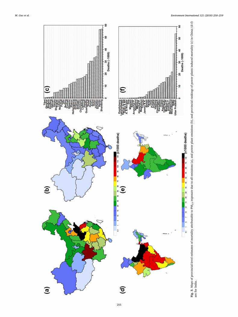
Fig.

3.Map

sof

prov

incial-le

vele

stim

ates

ofmortalityattributab

leto

PM2.5expo

sure

dueto

alle

mission

s(a),an

dpo

wer

plan

temission

s(b),an

dprov

incial

rank

ings

ofpo

wer

plan

tsindu

cedmortality(c)in

China

;(d–

f)areforIndia.

M. Gao et al. Environment International 121 (2018) 250–259

255

3.3. Mortality and YLL attributable to PM2.5 exposure

Estimates of mortality attributable to PM2.5 exposure due to allemissions and power generation emissions in China and India are listedin Table 2. The 95% uncertainty confidence intervals (CIs) are calcu-lated based only on the uncertainties of IER curve parameters. Othersources of uncertainty, such as the uncertainty in air quality modeling(emissions, model setup, etc.), population datasets and the fundamentaluncertainties inherent in applying a concentration-response functiondeveloped largely on the basis of epidemiology conducted in the US andWestern Europe at much lower concentrations than those now pre-valent in China and India to populations with a different genetic ma-keup, access to health care, diet and so forth to predict risks in Chinaand India (Dockery and Evans, 2017), are not included. Total ambientPM2.5 concentrations resulting from all sources would have led to1331.1 (95% Confidence Interval: 824.8–1914.6) thousand deaths at-tributable to PM2.5 exposure in China in 2013. Large fractions of theeffect come from stoke, IHD and COPD diseases.

Power plants are responsible for approximately 39% of ambientPM2.5 across China, and therefore are responsible for this share of themortality attributable to PM2.5 exposure – some 500 thousand annualdeaths (CI: 320 to 750 thousand deaths). However, because of the non-linearity in the IER, replacing all traditional coal-fired power genera-tion in China with clean energy sources would be expected to reducethe mortality attributable to PM2.5 by a fraction less than this value(Lelieveld et al., 2015). Of course, if such a strategy were coupled withother aggressive air pollution controls, the mortality benefits of repla-cing power plants with clean energy could be significantly larger.

In India, ambient PM2.5 concentrations resulting from all sources areprojected to be responsible for 803.8 (493.3–1135.2) thousand pre-mature deaths. Specifically, COPD contributes about 37.4%, IHD isresponsible for 23.8%, LRI contributes about 21.2%, stroke (both is-chemic and hemorrhagic) contributes about 15.3%, with a negligiblecontribution from LC. Emissions from power generation account forabout 60% of total SO2 emissions in India, but their influence on am-bient PM2.5 concentrations (accounting for only 32% of PM2.5 mass) islower than in China (where power plant emissions account for 39% ofPM2.5 mass).

Provincial health impacts attributable to PM2.5 exposure depend onboth population and ambient PM2.5 concentrations. In China, theBeijing-Tianjin-Hebei (BTH), the Yangtze River Delta (YRD), the PearlRiver Delta (PRD), and the Sichuan Basin (SCB) are densely populated(Fig. S6). In India, the IGP and east India are densely populated. Asshown in Fig. 2(a), the BTH (and Shandong, Henan provinces), YRD andthe SCB regions in China, and the IGP region in India exhibit the highestPM2.5 exposure. Fig. 3(a, d) shows the distributions of mortality attri-butable to PM2.5 exposure by province, in China and India. Shandong,Henan and Sichuan provinces in China, and Uttar Pradesh state in Indiaexhibit the largest mortality impacts of PM2.5. When attention is fo-cused on the impacts of emissions from power generation, Shandongand Henan provinces show the largest impacts in China (Fig. 3(b, c)). InIndia, the largest impacts of power plants are evident in the state ofUttar Pradesh (Fig. 3(e, f)).

Estimates of YLL attributable to PM2.5 exposure due to all emissions

and power generation emissions in China and India are summarized inTable 3. In China, the estimated YLL attributable to PM2.5 concentra-tions due to all sources are about 38.9 million years. In India, the totalYLL number attributable to PM2.5 exposure is only slightly lower (32.3million) than in China, in contrast to the large dissimilarity in mortality.

The calculations of YLL involve age specific life expectancy. In thisstudy, we take the average based on the distributions of ages in thepopulations. Since the birth rate in India is higher than in China, and itspopulation is younger, the remaining life expectancy (L) value for Indiafor all-age disease is higher than for China. This leads to high numbersof YLL attributable to PM2.5 exposure. In India, power generationemissions contribute about 33.1% of the YLL attributable to PM2.5 ex-posure. Fig. 4 shows the spatial distributions of provincial-level esti-mates of YLL attributable to PM2.5 exposure due to all emissions andpower generation emissions in China and India. Similar to the spatialdistributions of mortality attributable to PM2.5 exposure, Shandong,Henan and Sichuan provinces in China and Uttar Pradesh state in Indiaexhibit the largest YLL.

4. Discussion

4.1. Comparing health impacts with other studies

Several previous studies have estimated the mortality attributable toPM2.5 exposure in China and India (GBD MAPS Working Group, 2016;Ghude et al., 2016; Lelieveld et al., 2015; Liu et al., 2016), and ourestimates, 1.3 million deaths in China and 0.8 million deaths in India in2013, are consistent with the findings of these previous studies(Table 4).

When viewed in the context of the likely uncertainty in any of theseestimates, the differences among the many estimates are relativelyminor – especially considering that the studies used a variety of emis-sions estimates, atmospheric fate and transport models, and (to someextent) different syntheses of the epidemiological literature linkingPM2.5 exposure to mortality.

It may be of interest that although the estimates of the total mor-tality impact of PM2.5 exposure are similar across all studies, there aredifferences in the relative importance of various causes of death. Themore recent studies, which rely on the 2015 IER, tend to find greaterimpacts on COPD disease and smaller impacts on stroke. This is a re-flection of differences between the IER 2015 parameter estimates fromthe 2010 and 2013 versions of the IER. It is also worth noting that therole of ambient PM2.5 in the development of COPD is generally con-sidered to be uncertain (Schikowski et al., 2013).

Even using the same GBD framework (GBD 2015), estimates candiffer. Cohen et al. (2017) estimated 1108.1 thousand deaths attribu-table to PM2.5 (LRI: 66.3, LC: 146.0, IHD: 291.8, COPD: 281.7, andStroke: 322.3) in China and 1090.4 thousand deaths attributable toPM2.5 (LRI: 200.7, LC: 22.5, IHD: 365.6, COPD: 349.0, Stroke: 152.5) inIndia in 2015. In our study, the fractions of each disease in all-causedeath are similar to Cohen et al. (2017), but the all-cause deaths arehigher in China (1331.1 thousand), and lower in India (803.8 thou-sand).

The differences of annual mean PM2.5 concentrations in 2015 and

Table 3Estimated YLL attributable to PM2.5 concentrations due to all sources and power plant emissions over China in 2013 (95% uncertainty intervals are based on IERparameters) (million).

Stoke IHD COPD LC LRI Total

ChinaAll sources 5.6 (3.1–8.1) 6.0 (3.6–9.2) 16.3 (10.6–22.5) 7.1 (5.0–9.0) 3.9 (3.9–4.7) 38.9 (25.2–53.5)POW 2.2 (1.2–3.2) 2.4 (1.4–3.6) 6.2 (4.1–8.5) 2.8 (2.0–3.6) 1.5 (1.2–1.8) 15.1 (9.9–20.7)

IndiaAll sources 1.7 (0.9–2.5) 2.8 (1.6–4.3) 17.1 (10.5–23.9) 1.0 (0.7–1.4) 9.7 (7.2–12.0) 32.3 (20.9–44.1)POW 0.6 (0.3–0.8) 0.9 (0.5–1.4) 5.7 (3.5–7.9) 0.3 (0.2–0.5) 3.2 (2.4–4.0) 10.7 (6.9–14.6)

M. Gao et al. Environment International 121 (2018) 250–259

256

Fig.

4.Map

sof

prov

incial-le

vele

stim

ates

ofYLL

attributab

leto

PM2.5expo

sure

dueto

alle

mission

s(a),an

dpo

wer

plan

temission

s(b),an

dprov

incial

rank

ings

ofpo

wer

plan

tsindu

cedYLL

(c)inChina

;(d–

f)areforIndia.

M. Gao et al. Environment International 121 (2018) 250–259

257

2013 are likely to represent the major cause for these disparities. From2013 to 2015, PM2.5 concentrations in China decreased significantly(Clean Air Alliance of China, 2016) because of the strict air pollutioncontrol measures taken since 2013. The emission inventory used forIndia is based on the year 2010 in this study, so it might have led tounderestimations of all-cause deaths, and lower results for India thanCohen et al. (2017).

Large uncertainties are embodied in the calculations of source sectorcontributions because of the uncertainties in emission inventories, anddifferent responses to emission perturbations in different atmosphericchemistry models. Lelieveld et al. (2015) concluded that residentialenergy was dominant in outdoor air pollution in 2010 in both China(32%) and India (50%), while industry accounted for only 8% in Chinaand 7% in India. Both the GBD MAPS study and this study found thatindustrial sources are the largest sectoral contributor to air pollution inChina. The differences result very likely from the dissimilarities in theemission inventories employed, and partially from the differences ofatmospheric chemistry models. Lelieveld et al. (2015) used the Emis-sion Database for Global Atmospheric Research (EDGAR), and thisstudy used a state-of-the-art emission inventory for Asia (MIX, Li et al.,2017). Table S4 shows the comparison between these two datasets andshows that NOx non-methane volatile organic compounds (NMVOC)and NH3 emissions differ greatly, which might have led to the dominantrole of the agriculture sector in the results of Lelieveld et al. (2015).EDGAR ignores primary PM2.5 emissions in the simulation, which couldshow an even larger contribution to PM2.5 than BC and OC, leading toreduced contributions from sectors with high primary PM2.5 emissions.Besides, the coarser global model resolution (~100 km×100 km) usedin Lelieveld et al. (2015) might have missed mesoscale informationimportant for assessments on a regional scale.

4.2. Limitations

Although a complex regional meteorology-chemistry model, a state-of-the-art emission inventory in Asia, and more accurate IER para-meters were used in this study compared to previous studies, there arestill a number of limitations, involving each step in the calculationprocedures. We used relatively high model resolution to represent re-gional pollution features (60 km) compared to ~100 km in Lelieveldet al. (2015), but 60 km is still not good for precipitation simulations,and detailed urban and sub-grid information might have been missed.In this study, we need to run six one-year simulations (Table S2), andused 60 km due to computational limitations. Besides, we did not in-clude health impacts resulting from ozone exposure, mainly because themortality due to ozone exposure is small compared to that from PM2.5

(Ghude et al., 2016).Second, although thorough and detailed energy use information was

used in the development of the emission inventories, there is still agreat deal of uncertainty related to emission estimates from powerplants and other sectors. The uncertainties for different species differgreatly, and uncertainties for particles are much larger than those forgases. For example, the uncertainties of BC and OC emissions in MIXare±208% and±258% in China, but uncertainties of SO2 and NOx

are only± 12% and±31% (Li et al., 2017). The uncertainties in

emissions will be propagated into the meteorology-chemistry modeling.In terms of the source attribution to power plants, the uncertainties arerelatively low because of low uncertainties in gases and the importanceof gases in power plant emissions. In addition, SO2 and NOx emissionsfrom power plants were constrained using satellite retrievals (Streetset al., 2013). Compared to the sector contributions in Lelieveld et al.(2015), we found that different inventories can lead to large differ-ences. Thus we used the most advanced emission estimates (MIX, Liet al., 2017) in this study.

Third, uncertainties also arise from chemistry-meteorology mod-eling, related to chemical reactions, atmospheric dispersion, and de-position. Although we use nationwide surface PM2.5 measurements toevaluate model performance, comparisons of other air pollutants, in-cluding SO2, NOx, VOCs, and ozone, were not presented due to in-accessibility of relevant measurements. Yet the WRF-Chem perfor-mance was comprehensively evaluated in China and India in manyprevious studies (Gao et al., 2015, 2016a, 2016b, 2016c, 2017; Marrapuet al., 2014), and the results were encouraging, increasing confidence toour findings. Atmospheric chemistry modeling is the only approach toexamine sector-specific contributions to exposure. Errors can be re-duced further with advances in modeling approaches.

Fourth, the GBD 2015 IER parameters used in this study representonly the current best understanding, which will be enhanced withregular GBD updates in the future. For example, the IERs were devel-oped based on observed cohort studies in the US, Canada, and westEurope (Cohen et al., 2017), implying large uncertainties when appliedto China and India. In addition, the province-specific health benefits donot quantify the effect of inter-province transport due to computationalcomplexity, which may be redressed in the future using source appor-tionment techniques embodied in atmospheric chemistry models.

5. Conclusion

We estimate province-specific mortality and YLL attributable toambient PM2.5 exposure, and examine the changes in ambient PM2.5

and the health benefits expected to flow from eliminating power plantemissions, by combining atmospheric modeling and health impactanalyses. Several previous studies have evaluated the global mortalityattributable to PM2.5 exposure, but few have as yet explored the con-tributions of source classes.

The mortality burdens attributable to PM2.5 are estimated to be 1.3million in China and 0.8 million in India, which are consistent withprevious studies. We further quantified the impact of power generationemissions and found that power generation emissions contribute to 0.5million death in China and 0.3 million in India. We estimated also that15 million (95% Confidence Interval (CI): 10 to 21 million) years of lifelost can be avoided in China each year and 11 million (95% CI: 7 to 15million) in India by eliminating power generation emissions. The spa-tial distribution of these results reveals that priorities in upgradingexisting power generating technologies should be given to Shandong,Henan, and Sichuan provinces in China, and Uttar Pradesh state inIndia due to their dominant contributions to the current health risks.

Table 4Summary of Health Impacts from This Study and Other Studies.

Author Year analyzed Sources China India

Deaths (million) YLL (million) Deaths (million) YLL (million)

Lelieveld et al. (2015) 2010 All 1.4 0.6Ghude et al. (2016) 2011 All – 0.6Liu et al. (2016) 2013 All 0.9 –This study 2013 All 1.3 38.9 0.8 32.3HEI China MAPS, 2017 2015 All 1.1

M. Gao et al. Environment International 121 (2018) 250–259

258

Acknowledgements

We would like to acknowledge Professor John Evans at HarvardSchool of Public Health for insightful discussion and helpful comments;we thank Dr. Aaron J. Cohen and Dr. Richard T. Burnett for providingthe latest version IER parameters. We are grateful also to the ChinaNational Environmental Monitoring Center (CNEMC) and the Modelingof Atmospheric Pollution and Networking (MAPAN) groups for main-taining the high quality measurements of air pollutants in China andIndia. This study was supported by the Harvard Global Institute (HGI)fund, Harvard University, USA.

Appendix A. Supplementary data

Supplementary data to this article can be found online at https://doi.org/10.1016/j.envint.2018.09.015.

References

Beig, Gufran, Chate, D.M., Sahu, S.K., Parkhi, N.S., Srinivas, R., Ali, K., Ghude, S.D.,Yadav, S., Trimbake, H.K., 2015. System of Air Quality Forecasting and Research(SAFAR-India), GAW Report No. 217, World Meteorological Organization. GlobalAtmosphere Watch, Geneva, Switzerland.

Brauer, M., Amann, M., Burnett, R.T., Cohen, A., Dentener, F., Ezzati, M., Henderson, S.B.,Krzyzanowski, M., Martin, R.V., Dingenen, R., Donkelaar, A., Thurston, G.D., 2012.Exposure assessment for estimation of the global burden of disease attributable tooutdoor air pollutionEnviron. Sci. Technol. 46, 652–660.

Buonocore, J.J., Dong, X., Spengler, J.D., Fu, J.S., Levy, J.I., 2014. Using the CommunityMultiscale Air Quality (CMAQ) model to estimate public health impacts of PM2.5 fromindividual power plants. Environ. Int. 68, 200–208. https://doi.org/10.1016/j.envint.2014.03.031.

Burnett, R.T., Pope, C.A., Ezzati, M., Olives, C., Lim, S.S., Mehta, S., 2014. An integratedrisk function for estimating the global burden of disease attributable to ambient fineparticulate matter exposure. Environ. Health Perspect. 3, 397–404.

Chou, M.-D., Suarez, M.J., Ho, C.-H., Yan, M.M.-H., Lee, K.-T., 1998. Parameterizationsfor cloud overlapping and shortwave single-scattering properties for use in generalcirculation and cloud ensemble models. J. Clim. 11, 202–214.

Clean air alliance of China, 2016. CAAC Clean Air Management Report (2016).Cohen, A.J., Brauer, M., Burnett, R., Anderson, H.R., Frostad, J., Estep, K., et al., 2017.

Estimates and 25-year trends of the global burden of disease attributable to ambientair pollution: an analysis of data from the Global Burden of Diseases Study 2015.Lancet 389, 1907–1918. https://doi.org/10.1016/S0140-6736(17)30505-6.

Dockery, D.W., Evans, J.S., 2017. Tallying the bills of mortality from air pollution. Lancet389 (10082), 1862–1864.

Dockery, D.W., Pope, C.A., Xu, X., Spengler, J.D., Ware, J.H., Fay, M.E., Ferris Jr., B.G.,Speizer, F.E., 1993. An association between air pollution and mortality in six UScities. N. Engl. J. Med. 329 (24), 1753–1759.

Emmons, L.K., Walters, S., Hess, P.G., Lamarque, J.-F., Pfister, G.G., Fillmore, D., et al.,2010. Description and evaluation of the model for ozone and related chemical tra-cers, version 4 (MOZART-4). Geosci. Model Dev. 3, 43–67. https://doi.org/10.5194/gmd-3-43-2010.

Fann, N., Fulcher, C.M., Baker, K., 2013. The recent and future health burden of airpollution apportioned across U.S. sectors. Environ. Sci. Technol. 47, 3580–3589.https://doi.org/10.1021/es304831q.

Gao, M., Guttikunda, S.K., Carmichael, G.R., Wang, Y., Liu, Z., Stanier, C.O., et al., 2015.Health impacts and economic losses assessment of the 2013 severe haze event inBeijing area. Sci. Total Environ. 511C, 553–561. https://doi.org/10.1016/j.scitotenv.2015.01.005.

Gao, M., Carmichael, G.R., Wang, Y., Saide, P.E., Yu, M., Xin, J., et al., 2016a. Modelingstudy of the 2010 regional haze event in the North China Plain. Atmos. Chem. Phys.16, 1673–1691. https://doi.org/10.5194/acp-16-1673-2016.

Gao, M., Carmichael, G.R., Saide, P.E., Lu, Z., Yu, M., Streets, D.G., et al., 2016b.Response of winter fine particulate matter concentrations to emission and meteor-ology changes in North China. Atmos. Chem. Phys. Discuss. 1, 1–38. https://doi.org/10.5194/acp-2016-429.

Gao, M., Carmichael, G.R., Wang, Y., Ji, D., Liu, Z., Wang, Z., 2016c. Improving simu-lations of sulfate aerosols during winter haze over Northern China: the impacts ofheterogeneous oxidation by NO2. Front. Environ. Sci. Eng. 10, 1–11. https://doi.org/10.1007/s11783-016-0878-2.

Gao, M., Saide, P.E., Xin, J., Wang, Y., Liu, Z., Wang, Y., et al., 2017. Estimates of healthimpacts and radiative forcing in winter haze in eastern China through constraints ofsurface PM2.5 predictions. Environ. Sci. Technol. 51, 2178–2185. https://doi.org/10.1021/acs.est.6b03745.

GBD MAPS Working Group, 2016. Burden of Disease Attributable to Coal-burning andOther Air Pollution Sources in China|Health Effects Institute.

Ghude, S.D., Chate, D.M., Jena, C., Beig, G., Kumar, R., Barth, M.C., et al., 2016.Premature mortality in India due to PM2.5 and ozone exposure. Geophys. Res. Lett.43, 4650–4658. https://doi.org/10.1002/2016GL068949.

Greenland, S., Robins, J.M., 1991. Empirical-Bayes adjustments for multiple comparisonsare sometimes useful. Epidemiology 2, 244–251.

Grell, G.a., Peckham, S.E., Schmitz, R., McKeen, S.a., Frost, G., Skamarock, W.C., et al.,

2005. Fully coupled “online” chemistry within the WRF model. Atmos. Environ. 39,6957–6975. https://doi.org/10.1016/j.atmosenv.2005.04.027.

Guenther, A.B., Jiang, X., Heald, C.L., Sakulyanontvittaya, T., Duhl, T., Emmons, L.K.,et al., 2012. The model of emissions of gases and aerosols from nature version 2.1(MEGAN2.1): an extended and updated framework for modeling biogenic emissions.Geosci. Model Dev. 5, 1471–1492. https://doi.org/10.5194/gmd-5-1471-2012.

Hoek, G., Krishnan, R.M., Beelen, R., Peters, A., Ostro, B., Brunekreef, B., Kaufman, J.D.,2013. Long-term air pollution exposure and cardio-respiratory mortality: a review.Environ. Health 12 (1), 43.

Hong, Song-You, Noh, Yign, Dudhia, J., 2006. A new vertical diffusion package with anexplicit treatment of. Mon. Weather Rev. 134, 2318–2341.

Hu, J., Huang, L., Chen, M., Liao, H., Zhang, H., Wang, S., Zhang, Q., Ying, Q., 2017.Premature mortality attributable to particulate matter in China: source contributionsand responses to reductions. Environ. Sci. Technol. 51 (17), 9950–9959.

Huang, R.-J., Zhang, Y., Bozzetti, C., Ho, K.-F., Cao, J.-J., Han, Y., et al., 2014. Highsecondary aerosol contribution to particulate pollution during haze events in China.Nature. https://doi.org/10.1038/nature13774.

Kurokawa, J., Ohara, T., Morikawa, T., Hanayama, S., Janssens-Maenhout, G., Fukui, T.,et al., 2013. Emissions of air pollutants and greenhouse gases over Asian regionsduring 2000–2008: regional emission inventory in ASia (REAS) version 2. Atmos.Chem. Phys. 13, 11019–11058. https://doi.org/10.5194/acp-13-11019-2013.

Lelieveld, J., Evans, J.S., Fnais, M., Giannadaki, D., Pozzer, A., 2015. The contribution ofoutdoor air pollution sources to premature mortality on a global scale. Nature.https://doi.org/10.1038/nature15371.

Levy, J.I., Spengler, J.D., 2002. Modeling the benefits of power plant emission controls inMassachusetts. J. Air Waste Manage. Assoc. 52, 5–18. https://doi.org/10.1080/10473289.2002.10470753.

Levy, J.I., Spengler, J.D., Hlinka, D., Sullivan, D., Moon, D., 2002. Using CALPUFF toevaluate the impacts of power plant emissions in Illinois: model sensitivity and im-plications. Atmos. Environ. 36, 1063–1075. https://doi.org/10.1016/S1352-2310(01)00493-9.

Levy, J.I., Baxter, L.K., Schwartz, J., 2009. Uncertainty and variability in health-relateddamages from coal-fired power plants in the United States. Risk Anal. 29, 1000–1014.https://doi.org/10.1111/j.1539-6924.2009.01227.x.

Li, M., Zhang, Q., Kurokawa, J.I., Woo, J.H., He, K., Lu, Z., et al., 2017. MIX: a mosaicAsian anthropogenic emission inventory under the international collaboration fra-mework of the MICS-Asia and HTAP. Atmos. Chem. Phys. 17, 935–963. https://doi.org/10.5194/acp-17-935-2017.

Lim, S.S., Vos, T., Flaxman, A.D., Danaei, G., Shibuya, K., Adair-Rohani, H., et al., 2012. Acomparative risk assessment of burden of disease and injury attributable to 67 riskfactors and risk factor clusters in 21 regions, 1990–2010: a systematic analysis for theGlobal Burden of Disease Study 2010. Lancet 380, 2224–2260. https://doi.org/10.1016/S0140-6736(12)61766-8.

Lin, Yuh-Lang, Farley, Richard D., Orville, H.D., 1983. Bulk parameterization of the snowfield in a cloud model. J. Clim. Appl. Meteorol. 22, 1065–1092.

Liu, J., Han, Y., Tang, X., Zhu, J., Zhu, T., 2016. Estimating adult mortality attributable toPM2.5 exposure in China with assimilated PM2.5 concentrations based on a groundmonitoring network. Sci. Total Environ. 568, 1253–1262. https://doi.org/10.1016/j.scitotenv.2016.05.165.

Lu, Z., Zhang, Q., Streets, D.G., 2011. Sulfur dioxide and primary carbonaceous aerosolemissions in China and India, 1996–2010. Atmos. Chem. Phys. 11, 9839–9864.https://doi.org/10.5194/acp-11-9839-2011.

Marrapu, P., Cheng, Y., Beig, G., Sahu, S., Srinivas, R., Carmichael, G.R., 2014. Air qualityin Delhi during the commonwealth games. Atmos. Chem. Phys. 14, 10619–10630.https://doi.org/10.5194/acp-14-10619-2014.

Mlawer, E.J., Taubman, S.J., Brown, P.D., Iacono, M.J., Clough S A., 1997. Radiativetransfer for inhomogeneous atmospheres: RRTM, a validated correlated-k model forthe longwave. J. Geophys. Res. 102, 16663. https://doi.org/10.1029/97JD00237.

Randerson, J.T., van der Werf, G.R., Giglio, L., Collatz, G.J., Kasibhatla, P.S., 2015. GlobalFire Emissions Database, Version 4, (GFEDv4). ORNL DAAC, Oak Ridge, Tennessee,USA. https://doi.org/10.3334/ORNLDAAC/1293.

Robins, J.M., Greenland, S., 1989. Estimability and estimation of excess and etiologicfractions. Stat. Med. 8, 845–859.

Schikowski, T., Mills, I.C., Anderson, H.R., Cohen, A., Hansell, A., Kauffmann, F., Krämer,U., Marcon, A., Perez, L., Sunyer, J., Probst-Hensch, N., 2013. Ambient air pollution-acause for COPD? Eur. Respir. J. 43, 250–263. https://doi.org/10.1183/09031936.00100112.

Singh, N., Murari, V., Kumar, M., Barman, S.C., Banerjee, T., 2017. Fine particulates overSouth Asia: review and meta-analysis of PM2.5 source apportionment through re-ceptor model. Environ. Pollut. 223, 121–136. https://doi.org/10.1016/j.envpol.2016.12.071.

Streets, D.G., Canty, T., Carmichael, G.R., De Foy, B., Dickerson, R.R., Duncan, B.N., et al.,2013. Emissions estimation from satellite retrievals: a review of current capability.Atmos. Environ. 77, 1011–1042. https://doi.org/10.1016/j.atmosenv.2013.05.051Review.

van Donkelaar, A., Martin, R.V., Brauer, M., Boys, B.L., 2015. Global fine particulatematter concentrations from satellite for long-term exposure assessment. Environ.Health Perspect. 123, 135–143. https://doi.org/10.1289/ehp.1408646.

Xie, R., Sabel, C.E., Lu, X., Zhu, W., Kan, H., Nielsen, C.P., et al., 2016. Long-term trendand spatial pattern of PM2.5 induced premature mortality in China. Environ. Int. 97,180–186. https://doi.org/10.1016/j.envint.2016.09.003.

Zaveri, R.a., Peters, L.K., 1999. A new lumped structure photochemical mechanism forlarge-scale applications. J. Geophys. Res. 104, 30387. https://doi.org/10.1029/1999JD900876.

Zaveri, R.a., Easter, R.C., Fast, J.D., Peters, L.K., 2008. Model for simulating aerosol in-teractions and chemistry (MOSAIC). J. Geophys. Res. 113, D13204. https://doi.org/10.1029/2007JD008782.

M. Gao et al. Environment International 121 (2018) 250–259

259

View publication statsView publication stats