UNITED NATIONS CONFERENCE ON TRADE AND DEVELOPMENT

POLICY ISSUES IN INTERNATIONAL TRADE AND COMMODITIES

STUDY SERIES No. 45

THE IMPACT OF REMOVAL OF ATC QUOTAS ON INTERNATIONAL TRADE IN TEXTILES AND APPAREL

by

Marco Fugazza UNCTAD

and

Patrick Conway

University of North Carolina

UNITED NATIONS 

New York and Geneva, 2010 

ii

Note

The purpose of this series of studies is to analyse policy issues and stimulate discussions in the area of international trade and development. The series includes studies by UNCTAD staff, as well as by distinguished researchers from academia. In keeping with the objective of the series, authors are encouraged to express their own views, which do not necessarily reflect the views of the UNCTAD secretariat or its member States.

The designations employed and the presentation of the material do not imply the expression of any opinion whatsoever on the part of the United Nations Secretariat concerning the legal status of any country, territory, city or area, or of its authorities, or concerning the delimitation of its frontiers or boundaries.

Material in this publication may be freely quoted or reprinted, but acknowledgement is requested, together with a reference to the document number. It would be appreciated if a copy of the publication containing the quotation or reprint were sent to the UNCTAD secretariat at the following address:

Chief

Trade Analysis Branch Division on International Trade in Goods and Services, and Commodities

United Nations Conference on Trade and Development Palais des Nations CH-1211 Geneva

Switzerland

Series editor: Khalilur Rahman

Chief, Trade Analysis Branch

UNCTAD/ITCD/TAB/45

UNITED NATIONS PUBLICATION

ISSN 1607-8291

© Copyright United Nations 2010 All rights reserved

iii

Abstract

Theory predicts that a system of bilateral quotas such as observed in the Agreement on Textiles and Clothing (ATC) will cause both trade diversion and trade deflection, with an end result of more trading partners and smaller values traded on average than in the absence of the quotas. Quota removal will reverse this process, leading to trade creation and the focusing of trade in larger values by a smaller group of exporters.

We test these predictions in a model of bilateral trade among 128 world trading partners in

cotton textiles and apparel. We build a microfounded model of bilateral imports and estimate this model for those countries over the period 1997–2004. We find evidence of both trade diversion and trade deflection in this period governed by quotas.

The quota system was largely removed at the beginning of 2005. We use the model estimated

for the quota system years to predict bilateral trade in textiles and apparel in 2005 (out of sample). We do not find evidence of trade focus on average. This aggregate non-result is shown to be due to the averaging of the anticipated trade creation effect among a small group of low comparative cost exporters and the opposite, trade rediverting, effect among a larger group of countries displaced from sales in the United States and the European Union (EU) by the removal of quotas.

Key words: Quotas, trade models, heterogeneous firms, gravity

JEL Classification: F12, F13, F14

iv

Acknowledgements

This research was begun while Patrick Conway was a visitor at the UNCTAD headquarters in Geneva, and he thanks the Trade Analysis Branch for its hospitality and support during that time. Thanks to Michiko Hayashi for comments on an earlier version.

v

Contents

I. Characteristics of restraints on textiles and apparel imports to the United States and the EU ..........................................................................................3 II. Patterns of bilateral trade in textiles and apparel.............................................................5 A. Great variation in number of exports partners .............................................................5 B. Positive correlation of export markets and mean value of exports ..............................7 III. Modelling the bilateral import-export decision.................................................................9 A. Consumer demand........................................................................................................9 B. Producer characteristics ...............................................................................................9 C. Equilibrium in country j for variety v ........................................................................11 D. Deriving the value of bilateral trade...........................................................................11 E. Parameterizing the heterogeneity of exporting firms.................................................12 F. Implications of imposition of country-specific quotas by country j ..........................13 IV. Identification strategy for empirical estimation ..............................................................14 V. Estimation results...............................................................................................................17 A. Preliminary estimation: cost competitiveness in 1997 ...............................................17 B. Estimating the pattern of bilateral trade .....................................................................17 C. Estimating the value of bilateral trade........................................................................22 VI. Linking the two sectors ......................................................................................................26 VII. Predicting the effect of removing quota restrictions.......................................................27 VIII. Conclusions and extensions ...............................................................................................32 Bibliography ....................................................................................................................................33 Appendix 1 Trade focus – and trade deflection........................................................................35 Appendix 2 Measuring the quota system..................................................................................36 Appendix 3 Comparison of 2005 to pre-2005 average pattern of trade and value of trade: unconditional measure ..........................................................................................38

vi

List of figures

Figure 1. Textile and apparel trade in 2004................................................................................ 5 Figure 2. Textiles in 2004: number of export destinations and average value ........................... 7 Figure 3. Apparel in 2004: number of export destinations and average value ........................... 8

List of tables Table 1. Number of countries receiving textiles exports (by major exporter) .......................... 6 Table 2. Number of countries receiving apparel exports (by major exporter) .......................... 6 Table 3. Probit estimation of determinants of positive trade for SITC 652 ............................ 18 Table 4. Economies whose quality-adjusted cost differentials for 1998–2004 deviate significantly on average from the ĉi ranking in 1997 ................................................ 19 Table 5. How well do we predict (in-sample) the pattern of trade in textiles? ....................... 20 Table 6. Probit estimation of determinants of positive trade for SITC 841/842 ..................... 21 Table 7. How well do we predict (in sample) the pattern of trade in apparel?........................ 21 Table 8. Estimation results for textiles (SITC 652)................................................................. 22 Table 9. Estimation results for apparel (SITC 841/842) ......................................................... 24 Table 10. Estimation results for apparel (SITC 841/842) accounting for links to textiles (SITC 652) .................................................................................................... 25 Table 11. Proportion of non-zero bilateral trade pairs in sample (128 countries)..................... 27 Table 12. The implications of the quota regime for trade ......................................................... 28 Table 13. Out-of-sample forecasts for the trade pattern in 2005............................................... 29 Table 14. Actual versus predicted trade in textiles in 2005 ...................................................... 30 Table 15. Actual versus predicted trade in apparel in 2005 ...................................................... 30 Table 16. The change in “normal” trade relations in 2005........................................................ 31 Appendix tables Table A1. Quota limits (and binding quotas) in 1997................................................................ 36 Table A2. Correlation of quota limits and binding quotas in textiles, 1997 .............................. 37 Table A3. Correlation of quota limits and binding quotas in apparel, 1997 .............................. 37 Table A4. Trade focus and trade diversification in textiles ....................................................... 38 Table A5. Trade focus and trade diversification in apparel ....................................................... 38

1

On 1 January 2005 the United States, Canada and the EU eliminated a system of bilateral quotas on imports of textiles and apparel established by the ATC of the World Trade Organization (WTO) during the period 1995–2004. While these quotas were welfare reducing for the residents of these areas, they also had the effect of stimulating exports of textiles and apparel from a number of developing economies that might otherwise not have participated in those import markets. This effect is “trade diversion”, as Viner (1950) characterized it, for the importing countries and a growth stimulus for the developing country exporters. There is also the potential for “trade deflection” and “trade destruction”, as Bown and Crowley (2007) predict: countries facing a binding quota from these areas will then either deflect their products to third countries or reduce their imports from third countries by substituting domestic production.

In this paper we investigate these hypotheses about trade flows. We create a microfounded model of trade flows using the heterogeneous firm approach of Helpman et al. (2007). We estimate this model in the quota period 1997–2004 for a sample of 128 developed and developing countries, and then use the removal of quotas in 2005 as an experiment to identify the refocusing of trade predicted by theory relative to the pattern of the quota period model. This out-of-sample exercise yields quantitative predictions of patterns and volumes of trade that we compare to the actual realizations. While we do not measure welfare effects explicitly, we are able to track the country-specific evolution in export expansion or contraction. We find that, contrary to theoretical predictions, the average number of trading partners rose between 2004 and 2005 and the average volume of trade was reduced. While the simple theory of trade creation suggests that there will be greater specialization and greater volume of trade per trading partner with the removal of trade barriers, the opposite is evident on average. The reason for this paradoxical result is evident once countries are separated by outcome. The “comparative advantage” exporters (including the major Asian exporters) in these two industries did reduce the number of trading partners and increase the average volume of trade per exporter, just as theory predicts. By contrast, the countries that became exporters of textiles and apparel because of the quota system did not shut down. Instead, they sold smaller volumes of their goods to more peripheral markets. The predicted outcomes from the sample are the average of these two effects, with the non-comparative advantage countries dominating the average.

Our attention to the general equilibrium and third country effects of removal of quotas distinguishes our work from two recent papers on the removal of the ATC quotas. Harrigan and Barrows (2006) examined the difference in price and quality for United States imports in a difference-in-difference framework for the top 20 exporters to the United States: there is the time difference, from 2004 to 2005, and the categorical difference in quota-constrained versus unconstrained imports.1 The authors first measure the average adjustment in price and quality for each country in the sample; they find a substantial downward average adjustment in price for quota-constrained imports and a much smaller downward adjustment in quality. There are no such downward adjustments for unconstrained imports. The authors then test across countries to determine whether the adjustments in price and quality from 2004 to 2005 are on average significantly different for constrained than for unconstrained categories. The downward price adjustments are statistically significant for all exporters at a 95 per cent level of confidence, for China alone and for the non-China exporters. The downward quality adjustments are significant for China alone and for all exporters at the 90 per cent level of confidence. This work is done at a quite detailed level of disaggregation, and signals the expected impact of quota removal on both price and quality. It treats the observation of a binding quota as an exogenous event, however – and this can introduce bias.

Brambilla et al. (2007) focus their attention on exporters of textiles and apparel to the United States. They work as well with 10-digit HS data on imports from these countries into the United States, and they also categorize the imports as being quota-constrained versus unconstrained using the

1 The unit for imports is the HS 10 classification. Each classification is designated as either “constrained” or “unconstrained” depending upon whether that classification is part of a quota category binding for that exporter in that year.

2

United States quota classifications. They analyse carefully the impact of the quota, and then contrast that with behaviour after quota removal: they are careful to distinguish the four stages of sequential quota elimination under the ATC, and to connect the changes in quantity and price with the appropriate stage of quota removal. They find both an increase in quantity and a reduction in price for Chinese goods that is significantly different from that observed in other quota-constrained exporters. They do not calculate quality as in Harrigan and Barrows (2006), and thus cannot draw conclusions on the impacts of price versus quality. They also treat the quota-constrained period as an exogenous event.

Our approach to the removal of quotas represents both an extension and an aggregation of the results of these two papers. We extend these conceptually by considering the general equilibrium effects of bilateral trade among all countries, not just those that impose quotas. We model the production/trade relationship between textiles and clothing. We also extend the analysis technically by recognizing that a binding quota will be an endogenous event in this model. We draw back from the disaggregation at the 10-digit HS level used by these two papers. As a result, we must create an indicator of quota limits and binding quotas based upon aggregating up from the individual quota categories defined by the United States and the EU. Details are provided in the text and data appendices.

3

I.   Characteristics of restraints on textiles and apparel imports to the United States and the EU 

The system of bilateral quantitative restraints (or quotas) on textile and apparel imports was an enduring feature of the United States and EU commercial policy system. From its inception in the early 1960s with the Long-Term Agreement regarding International Trade in Cotton Textiles (LTA), through its codification in the Multi Fibre Agreement (MFA) from 1974 to 1995, and to its 1995–2005 form in the ATC, the system provided protection to United States and EU producers of textiles and apparel.2

In the negotiations that led to the adoption of the ATC in 1995, the United States and EU agreed to dismantle the system of quantitative restraints sequentially. A large number of restraints were removed at the beginning of 1995, 1998 and 2002, but those remaining governed trade in the categories of textiles and apparel most produced in the United States and EU. These remaining restraints were removed on 1 January 2005. The ATC by its end had evolved into a complicated interlocking set of bilateral agreements on quantities exported. They acted as export restraints, but they were binding in any given year on only a small subset of the countries under restraint. Specific limits and group limits interacted in non-transparent ways to limit a given country’s exports.

The basic unit of the quota system was the restraint category, or quota category. These categories were defined as aggregated sub-groups of textile and apparel products with some shared characteristic or raw material. The system of import restraints defined by the United States identified 11 aggregated categories of yarns, 34 aggregated categories of textiles, 86 categories of apparel and 16 categories of miscellaneous textiles (e.g. towels). Together these categories spanned the entire set of United States textile and apparel imports. The EU identified 41 categories of yarns, 28 categories of textiles, 42 categories of apparel and 32 categories of miscellaneous textiles for a total of 143 categories – although some of these categories were further subdivided by raw material.3 Each category included multiple products. For example, United States category 225 (blue denim) was aggregated from 16 distinct HS product lines. Products included in each category were similar, but could have significant differences: for example, the “blue denim” category included denim made from both cotton and man-made fibres. There is no corresponding category for the EU: its blue denim imports would have been classified EU category 2 (woven cotton fabric, with 105 CN product lines) or EU category 3 (synthetic woven fabric, with 80 CN product lines).

Limits under the system of restraints were divided into specific limits and group limits. Specific limits governed the import of goods within the specific quota category. Group limits placed aggregate limits on a subset of the quota categories. If a country’s exports were subject to group limits but not specific limits, then the suppliers of that country (or more likely, a government agency supervising these exports) could choose any mix of goods shipped to the United States so long as in aggregate the totals did not exceed the group limit. Some group limits covered only two quota categories: e.g. United States group 300/301, covering United States quota categories 300 (carded cotton yarn) and 301 (combed cotton yarn). Others spanned a large number of categories: for example, Sub-group 1 in Hong Kong (China) included United States quota categories 200, 226, 313, 314, 315, 369 and 604. In many cases, a country had its exports bound by both specific limits and group limits.

2 Francois et al. (2007) provides a detailed discussion of this chronology. There were actually six groupings that imposed bilateral quotas under the MFA and ATC: in addition to the EU and the United States, there were Austria, Canada, Finland and Norway. The work in this paper focuses upon the United States and the EU, but the analysis will be extended to the others in future research. 3 The categories for the United States and the correspondence between those categories and the HS classification of imports are published by the Office of Textiles and Apparel (OTEXA), Department of Commerce, at http://otexa.ita.doc.gov/corr.htm. The categories for the EU and concordance with CN category are published in EEC Council Regulation 3030/93 of 12 October 1993.

4

Under the MFA and ATC, exporting countries were given flexibility in meeting these restraints. In each category, the agreement specified a percentage by which the country could either exceed or fall short of its restraint. In those cases, a maximum per cent of possible “carry-forward” or “carry-over” is specified in the agreement. With carry-over, the country transfers an unused part of the previous year’s quota to the current year. With carry-forward, the country exceeds its quota in the current period by counting the excess against quota in the following year.4

Not all textiles exporters were subject to quantitative limits. Under the MFA and ATC, restraints were negotiated whenever a country’s exports caused (or threatened to cause) market disruption in the United States or EU. Of the 152 countries exporting cotton knit shirts to the United States (United States categories 338 and 339) in 2004, only 32 were subject to quantitative limits and of these only 11 exported as much as 90 per cent of the quota limit to the United States. Similarly, of the 156 countries exporting knit shirts (cotton and other fabrics) to the EU in 2004, only 25 were subject to quantitative limits, and of those only four exported more than 90 per cent of the quota limit to the EU.

4 Information on flexibility is drawn from OTEXA (2003) and from EEC (2005).

5

II.  Patterns of bilateral trade in textiles and apparel 

We begin by examining the bilateral trade patterns in aggregate cotton textiles (SITC 652) and apparel (SITC 841 & 842) for 169 countries over the period 1997–2004.5 There are three salient features of international trading patterns evident in the data: the great variation in the number of trade partners by exporting country, the positive correlation between number of trade partners and mean value of exports and the distinctive patterns of trade partners brought about by the system of quotas.

A. Great variation in number of export partners

Figure 1 ranks each of the 169 countries in the sample in ascending order by the number of countries to which it exported in 2004 in these two trade classifications. It then indicates on the vertical axis the percentage of the 168 potential trading partners to which each country exports. In the apparel classification, there are four countries that report zero exports. The numbers then slowly rise, until for the country with the most partners (Italy) 86 per cent of the countries are destinations for their exports. In the textile classification, 12 countries report zero exports. The country with the most textile export markets (Italy, once again) exports to 83 per cent of the countries in the sample.

Figure 1. Textile and apparel trade in 2004

0

10

20

30

40

50

60

70

80

90

100

Ranked in ascending order by percent of other countries served through exports

Expo

rts

to th

is p

erce

nt o

f sam

ple

SITC 841 & 842 SITC 652

5 We have bilateral trade flows by year for 169 countries, but will reduce the sample to 128 countries later so that we will have access to necessary non-trade regressors.

6

While the focus of the debate over the elimination of the ATC has been on the flows of exports from Asia to the United States and the EU, Asian exporters are involved in sales to many more countries than these – in fact, to a majority of the countries in the sample. Table 1 indicates the number of countries receiving exports from seven major textiles exporters. The Asian countries have a market base that extends well beyond the 18 ATC quota-imposing countries. The United States is also a major exporter of its textiles.

Table 1. Number of countries receiving textiles exports (by major exporter)

China India Pakistan Republic of Korea Indonesia Viet Nam

United States

1997 115 107 98 97 79 22 114 1998 123 109 102 101 94 29 116 1999 126 115 107 105 93 34 119 2000 131 119 108 106 92 35 123 2001 132 126 113 103 95 32 123 2002 131 120 107 101 90 44 117 2003 130 117 116 104 89 47 117 2004 114 106 100 90 84 40 106 Source: COMTRADE database.

In table 2, a similar point is made even more emphatically for apparel. The seven Asian countries have customers in a great majority of the countries of the world – as do the United States.

Table 2. Number of countries receiving apparel exports (by major exporter)

China India Pakistan Republic of Korea Indonesia Viet Nam

United States

1997 110 102 61 80 96 58 112 1998 118 103 61 89 103 64 116 1999 126 101 66 90 101 65 121 2000 135 112 69 91 112 66 121 2001 138 116 75 95 112 71 126 2002 124 114 74 91 105 76 117 2003 129 110 75 92 108 77 120 2004 116 106 80 84 103 79 106 Source: COMTRADE database.

Most countries do not have this great diversification of exports – in fact, 92 per cent of apparel exporters and 90 per cent of textiles exporters sell to fewer than half the countries in the sample. The export business is also not driven solely by low labour cost: the lists of top 20 exporters in terms of number of markets served include a large number of developed countries.6

6 In apparel, six of the top 10 exporters in terms of numbers of trading partners are developed countries (Italy, Germany, France, Spain, the United Kingdom and the United States). In textiles, seven of the top 10 exporters in terms of numbers of trading partners (those above plus Belgium) are developed countries.

7

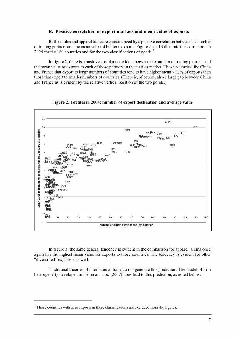
B. Positive correlation of export markets and mean value of exports

Both textiles and apparel trade are characterized by a positive correlation between the number of trading partners and the mean value of bilateral exports. Figures 2 and 3 illustrate this correlation in 2004 for the 169 countries and for the two classifications of goods.7

In figure 2, there is a positive correlation evident between the number of trading partners and the mean value of exports to each of those partners in the textiles market. Those countries like China and France that export to large numbers of countries tend to have higher mean values of exports than those that export to smaller numbers of countries. (There is, of course, also a large gap between China and France as is evident by the relative vertical position of the two points.)

Figure 2. Textiles in 2004: number of export destination and average value

ITA

DEUFRA

GBR

ESP

CHN

BEL

USA

IND

PAKHKG

TWN

AUT

KOR

THA

TUR

NLDPRT

IDNCHE

JPN

ARE

BRACZE

CANMYS

SWEZAFEGY

AUS

RUS

POLSGP

GRC

DNKBGRISRIRL

SVN

NORFIN

VNMLKA

PHL

MEX

EST

BGD

ROM

TUN

SYR

MAR

LTU

UZB

MUS

HUN

SVKPER

TKM

SAU

LVABLR

CHL

PRK

URY

NGA

BHR

UKR

TJK

NZL

COL

PAN

KEN

CIVMDA

ZWE

SEN

IRN

GHA

ARG

CYP

MLTMKD

GTM

MLI

MAC

HRV

ECU

TZA

LBN

KHM

ISL

MDGKAZETH

LUXPRY

NPL

NER

BEN

TTO

SLV

OMN

JOR

BFA

VEN

TGO

MRT

LAOCRI

HNDCMR

AFG

SLE

NIC

GMB

GEODOMBOL

BIHZMB

KGZFJICOGALB

ZARKWT

DJI

SUR

MWI

MOZ

MNG

MDV

JAM

CPV

BRNBRBAZE

ANT

YEM

TCD

SYCSDN

RWAQAT

PNG

LBR

GUY

GNB

ERI

DZA

DMA

CUB

BMU

BHS

BDI

ATG

ARM

-1

0

1

2

3

4

5

6

7

8

9

10

11

0 10 20 30 40 50 60 70 80 90 100 110 120 130 140 150

Number of export destinations (by exporter)

Mea

n va

lue

in lo

garit

hms

of th

ousa

nds

USD

of S

ITC

652

exp

orts

In figure 3, the same general tendency is evident in the comparison for apparel. China once again has the highest mean value for exports to those countries. The tendency is evident for other “diversified” exporters as well.

Traditional theories of international trade do not generate this prediction. The model of firm heterogeneity developed in Helpman et al. (2007) does lead to this prediction, as noted below.

7 Those countries with zero exports in these classifications are excluded from the figures.

8

Figure 3. Apparel in 2004: number of export destination and average value

ITADEU

FRA

CHN

ESPGBR

IND

USA

HKGIDN

THA

TUR

TWNARE

KORCANPAK

AUTCHE

VNM

NLDPHLDNK

JPN

BELLKA

ROMBGDMARTUN

POL

MYS

BGR

HUN

SGP

PRT

BRA

MAC

GRC

KHM

SVKUKR

MUS

MEX

EGYHRVSVNCZERUS

AUS

LTUSWE

SYR

MKD

ZAFISR

COL

MDG

PER

LVAFINIRL

NOR

BLRMLTNPL

ARG

LAO

SAU

CYP

BIHMDA

ECU

PAN

CHL

LBN

ESTALBPRK

KGZ

DOM

JOR

OMN

GTMHND

BOLPRY

SLV

NZL

KEN

LUX

CRI

IRN

URY

BHR

CMR

MNG

KWT

KAZ

VEN

NIC

ZWE

ISL

NGA

MRTGHA

QAT

TKMTJKUZB

ANT

FJI

SLE

DMASEN

AFG

JAMBRN

MDV

MOZ

ETH

TGO

GEOTTO

CIVTZA

YEM

BFA

ARM

ZAR

HTI

BLZ

LCAAZECUB

DZA

MWI

KNA

MLIBRBATG

CPVUGA

SURLBR

GMBSDNNER

PNGBENBMU

GUY

BHSCAFZMBCOG

COM

BDISTPGINVCTGAB

RWA

ERI

TCD

-1

0

1

2

3

4

5

6

7

8

9

10

11

12

13

0 10 20 30 40 50 60 70 80 90 100 110 120 130 140 150

Number of Export Destinations (by exporter)

Ave

rage

Val

ue o

f Exp

orts

(in

loga

rithm

s of

USD

thou

sand

s)

9

III.  Modelling the bilateral import‐export decision 

To identify the impact of quotas on the pattern and volume of bilateral trade, it is necessary to control for the other factors determining trade in these goods. In this section we provide a structural model of the decision to import from one country to another adapted from Helpman et al. (2008) to the features of world trade in textiles and apparel.

A. Consumer demand

In country j and in time t, each individual b consumes a quantity ξbjt(ν) of each variety of textiles (or apparel) from a continuum along the interval [0 β], with β the share of individual income spent on these varieties. He derives utility in a Dixit and Stiglitz (1977) aggregator as below:

Ubjt = {∫ ξbjt(ν)α dν}(1/α) 0 < α < 1 (1)

If Yjt = Σb Ybjt is the real income of country j in time t, aggregated from real income of each individual b, then the country j demand for variety ν is

pjt(ν) xjt(ν) = Σb ξbjt = pjt(ν)1-ε βYjt/Pjt1-ε (2)

Pjt = { ∫ pjt(ν)1-ε dν} 1/(1-ε) (3)

Where pjt(ν) is the average price of variety ν in country j at time t.8 Pjt is the sector’s ideal price index, and every product ν has a constant price elasticity ε = (1/(1-α)) defined to be positive. These goods could either be locally produced or produced in foreign countries, as noted below: within each variety ν, the products of different countries of the same quality are near-perfect substitutes to the consumer.

B. Producer characteristics

Suppliers create each variety ν through use of labour. The total cost of production for an individual supplier f is given in labour units as

Cfit(ν) = citaf(ν)xf(ν) + citFfit(ν) (4)

8 This derivation is appropriate for differentiated products with the same quality. If the differentiated products differ as well along a quality dimension, Hallak (2006) demonstrates that a similar derivation will hold with ξbjt and pjt(ν) defined in quality adjusted units. For example, if quality of goods from supplier i is defined θi and the price of product ν from supplier i to country j is pijt(ν) , then pjt(ν) xjt(ν) = (pijt(ν)/θi) 1-ε Yjt/Pjt

1-ε, where Pjt = { ∫ (pijt(ν)/θi) 1-ε dν} 1/(1-ε). We return to this point in the next section.

10

The first element of the summation is the variable cost, with xf(ν) as a measure of total production.9 The second element is the fixed cost of producing for export; it will be the summation of fixed costs for exporting to each of the supplier’s importing countries.10 For each variety ν there is a distribution of suppliers in each country. Supplier-level heterogeneity is decomposed into two parts. First, there is a global distribution of technology. We use labour input per unit of output (or the inverse of productivity) as the index, denoted by “a”. (Low values of “a” represent low cost, or high productivity, firms, and high values represent the converse.) All suppliers worldwide have technology defined by a supplier-specific draw af from the time-invariant distribution g(a) bounded in the range [aL aH]. Second, there is a country-level difference in production cost cit that scales up or down the productivity of all suppliers in that country. Consider a continuum of suppliers in country i at time t. The per-unit variable cost of each country i firm in time t is defined citaf(ν). Each supplier f in country i of variety ν will have unit cost vfit(ν) = cit af(ν) in selling in the domestic market. vijt(af(ν)) = cit af(ν) + Fijt(ν)/xf(ν) is the unit cost for goods exported to country j.11

Not all producers will export to all countries. Define Πijt(ν) as supplier profits due to exporting from country i to country j in period t. The zero profit condition in (5) defines the lowest productivity firm ao

ijt(ν) able to export variety ν to country j. A definition of this productivity level is derived from (5) and reported in (6).

Πijt(ν) = [pijt(ν)/[(1+sijt)(1+tijt)] – citaoijt(ν)] xf (ν) – citFijt(ν) = 0 (5)

{pijt(ν)/[cit(1+sijt)(1+tijt)]} - Fijt(ν)/ xf (ν) = aoijt(ν) (6)

sijt is the per cent shipping cost from country i to country j and tijt is the ad valorem tariff (or tariff equivalent of a non-tariff barrier) imposed by country j on the products of country i. As shipping costs, country-specific production costs, fixed costs or tariffs rise, the critical ao

ijt(ν) will fall (i.e. the necessary productivity level to be an exporter to j will rise). As average import price in country j pjt(ν) rises, ao

ijt(ν) will rise. For suppliers in country i with high productivity draws af < aoijt there will be non-

negative profits in exporting to country j; for firms with af > aoijt there will be no exporting to country j.

Since the cut-off differs by trading partner, those firms in country i unable to export to country j may be able to export to country k so long as ao

ijt < aoikt.

Note the important end-point restrictions. The calculation in (6) puts no limits on aoijt, but we

know that a is drawn from the range [aL aH]. If aoijt < aL, this indicates that none of the country i

suppliers can be profitable in selling to country j. If aoijt > aH, then all country i suppliers will be

profitable in selling in the country j market.

9 Given the producer’s technology, we assume that it is either producing at full capacity or not producing at all. 10 This fixed cost is exemplified by the distribution network that an exporter must establish prior to servicing a new market. 11 The total fixed cost Ffit = Σj Fijt, where j is summed over the set of countries to which the supplier exports.

11

C. Equilibrium in country j for variety ν

Demand for variety ν in country j is given by xjt(ν) in equation (2). Supply of variety ν to country j is determined by the individual firm’s zero profit condition in equation (5). As the price pjt(ν) at which the variety can be sold rises, ao

ijt(ν) rises. This increases (or at worst leaves constant) the number of suppliers in country i willing to export to country j.

The supply from country i to country j (Xijt) and the total supply to country j (Xjt) can be defined:

Xijt(ν) = aL ∫ aoijt(ν) xf(ν) g(a) da (7)

Xjt(ν) = Σi Xijt(ν) (8)

Note that both Xijt(ν) and Xjt(ν) are non-decreasing in the price pjt(ν) through the cut-off productivity values ao

ijt(ν).

Equilibrium in country j in the market for variety υ is defined by the equality of supply and demand:

Xjt(ν) = xjt(ν) (9)

The equilibrium pjt(ν) and aoijt(ν) are jointly determined through the zero profit condition for

each supplier country. This equilibrium is not determined in isolation: firms potentially supplying variety ν will also consider exporting to other countries, and will be competing for scarce resources with suppliers of other varieties – and other goods. The set {pjt(ν), ao

ijt(ν)} equilibrates to leave country i at full employment. We also anticipate that cit could adjust over time to achieve full employment: one interpretation of cit is as the prevailing wage in country i, exogenous to each firm but endogenous to the labour market of the country.

D. Deriving the value of bilateral trade

In this model, the landed (i.e. cif) value of textile imports of variety ν from i into j in time t is

Mijt = [pijt(ν)/(1+tijt)]xijt(ν) (10)

= [pijt(ν)/(1+tijt)]xjt(ν){xijt(ν)/xjt(ν)}

Mijt = Yjt Δijt(ν) Vijt(ν) (11)

Where Vijt(ν) = xijt(ν)/xjt(ν)

and Δijt = β (pijt(ν))/Pjt)1-ε/(1+tijt)

12

Bilateral trade values thus depend on three elements. The gross domestic product (GDP) of the importing country Yjt represents the purchasing power of the importing economy. Δijt represents the cost of imported variety ν from exporter i relative to other products available within the economy. Vijt(ν) measures the technological competitiveness of country i producers in the country j market, inclusive of the impact of tariff barriers to trade.12 If ao

ijt < aL, then xijt(ν) = 0 and Vijt(ν) = 0. As aoijt

rises above aL, the number of exporters from country i to country j will rise and the share Vijt(ν) will rise as well. As the number of exporters rise, so also does the value of trade. As the tariff rate rises, the landed value of imports will fall.

The correlation between the number of export markets served and the mean value of exports per export market follows from this theoretical feature of the model. Exporting countries with (for example) lower production cost (cit) will have higher cut-off productivity ao

ijt for all importers j. This leads both to export to more countries through (6) and to larger mean value of imports to those countries through (11).

E. Parameterizing the heterogeneity of exporting firms

In this model of international trade, it is quite important to consider explicitly the productivity of individual suppliers within an exporting country. The preceding section derived results for a general distribution function g(a). In this section, we will consider the implications of use of a specific distributional assumption for g(a).

We follow Helpman et al. (2007) in assuming that the global technology distribution function g(a) follows a constant Pareto distribution across time and country.

g(a) = κaµ-1/(aHµ – aL

µ) with shape parameter µ (12)

The distribution nests the uniform distribution as a special case with µ = 1, but also admits distributions skewed towards a higher marginal cost of production for µ > 1 and distributions skewed toward a lower marginal cost of production for µ < 1.

Given this parameterization, the variable Vijt from (11) can be rewritten as

Vijt = Wijt / Vojt (13)

with Vojt = Njt(ν)[(aojt/aL)µ – 1]

and Wijt ={(aoijt/aL)µ – 1} for ao

ijt > aL

= 0 otherwise

The definition of Vojt indicates that it is increasing in µ, ceteris paribus, and is a measure of the equilibrium volume for all suppliers to country j. Njt(ν) is the number of countries exporting variety ν to country j in period t. ao

jt(ν) is the “average” competitiveness of all suppliers to importer j in period t. Wijt is an indicator of the degree to which individual suppliers from country i are competitive in country j.

12 If we impose an assumption of equal capacity xf(ν) for all firms in all countries, then (xijt(ν)/xf(ν)) = aL∫aoijt(ν) g(a) da. We define the “average” competitiveness through definition of ao

jt(ν) such that (xjt(ν)/xf(ν)) = Nj(ν) aL∫aojt(ν) g(a) da, with Nj(ν) the number of countries with positive exports of ν to country j.

13

F. Implications of imposition of country-specific quotas by country j

The country j market is an imperfectly competitive one, but there are two reasons that pijt(υ) will diverge from the country j average pjt(υ). The first will be differences in quality. With quality denoted by θi for each exporter i, the equilibrium prices in importer j in period t will have the relation defined in (14).

pijt(υ)/ θi = pjt(υ) for each variety υ without quota (14)

pijt(υ)/ [θi pjt(υ)] = τijt τijt > 1 with quota (15)

The second will be the existence of binding quota restrictions imposed by country j on the exports of county i. If country j imposes binding quotas qkjt < xkjt on the quantity imported from country k in period t, then the value of imports from country k will be Mkjt = pkjtqkjt, not the optimal quantity defined by (2) for these goods. This will lead to the protection of domestic industry, the deadweight losses associated with quotas and a wedge between average price and quota-driven price as in (15). τijt is the value of the wedge created by a binding quota by country j on country i goods.

The quota may also lead to trade diversion, trade deflection and trade destruction. If country j originally imported only from country 1 but then imposed a quota on imports from that country, there will be a variety of efficiency losses. First, the binding quota excludes exports from country 1. Country j will import the quota amount from country 1, but its excess demand will spill over to other exporting countries. The spillover of demand due to the quota may raise the critical value for exporter k (ao

kjt) so that it is greater than aL and then the most productive firms in country k will sell to country j. The reduced demand by country j for country 1’s products may also increase the quantities exported by country 1 to other trading partners – and may in fact lead to initial exports to some countries not previously served.

Once quotas are imposed, the new pattern of trade includes imports from country 1 and other countries. Imports from another country k are a form of trade diversion as first propounded by Viner (1950), although in this case the diversion is due to a country-specific quantitative restriction rather than a customs union. There are thus two implications of imposition of the non-zero quota. First, there will be at least as many, and possibly more, countries exporting to the quota imposing importer. Second, the quantities imported from exporters subject to a binding quota will be strictly less. For ε > 1, the value of imports M1jt from country 1 subject to a binding quota will also be less.13 Exporters denied entry to the quota-imposing importers will also export more to other importing countries – the “trade deflection” described by Bown and Crowley (2007). They will import less of varieties of this good from third countries – the “trade destruction” of Bown and Crowley (2007).

Removing quotas should then generate fewer bilateral trading pairs, and greater average imports along remaining bilateral lines, for the countries removing the quotas. Third country exporters – those without comparative advantage in the absence of quotas – will export less to those countries removing the quotas. This could either lead to reduced production (as resources shift to exploit comparative advantage) or re-orientation of exports to other markets.

13 This is certainly the case in the model presented here. An alternative model will include quota rents in the exporting country. These rents will raise the rent-inclusive price of the export and could reverse the conclusion.

14

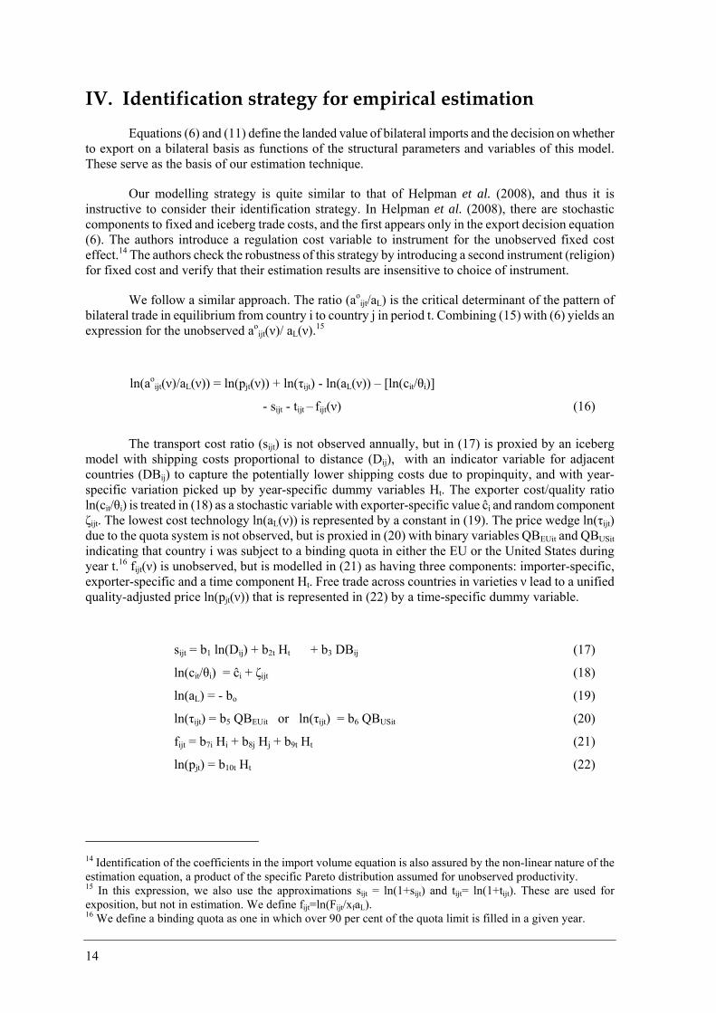
IV.  Identification strategy for empirical estimation 

Equations (6) and (11) define the landed value of bilateral imports and the decision on whether to export on a bilateral basis as functions of the structural parameters and variables of this model. These serve as the basis of our estimation technique.

Our modelling strategy is quite similar to that of Helpman et al. (2008), and thus it is instructive to consider their identification strategy. In Helpman et al. (2008), there are stochastic components to fixed and iceberg trade costs, and the first appears only in the export decision equation (6). The authors introduce a regulation cost variable to instrument for the unobserved fixed cost effect.14 The authors check the robustness of this strategy by introducing a second instrument (religion) for fixed cost and verify that their estimation results are insensitive to choice of instrument.

We follow a similar approach. The ratio (aoijt/aL) is the critical determinant of the pattern of

bilateral trade in equilibrium from country i to country j in period t. Combining (15) with (6) yields an expression for the unobserved ao

ijt(ν)/ aL(ν).15

ln(aoijt(ν)/aL(ν)) = ln(pjt(ν)) + ln(τijt) - ln(aL(ν)) – [ln(cit/θi)]

- sijt - tijt – fijt(ν) (16)

The transport cost ratio (sijt) is not observed annually, but in (17) is proxied by an iceberg model with shipping costs proportional to distance (Dij), with an indicator variable for adjacent countries (DBij) to capture the potentially lower shipping costs due to propinquity, and with year-specific variation picked up by year-specific dummy variables Ht. The exporter cost/quality ratio ln(cit/θi) is treated in (18) as a stochastic variable with exporter-specific value ĉi and random component ζijt. The lowest cost technology ln(aL(ν)) is represented by a constant in (19). The price wedge ln(τijt) due to the quota system is not observed, but is proxied in (20) with binary variables QBEUit and QBUSit indicating that country i was subject to a binding quota in either the EU or the United States during year t.16 fijt(ν) is unobserved, but is modelled in (21) as having three components: importer-specific, exporter-specific and a time component Ht. Free trade across countries in varieties ν lead to a unified quality-adjusted price ln(pjt(ν)) that is represented in (22) by a time-specific dummy variable.

sijt = b1 ln(Dij) + b2t Ht + b3 DBij (17)

ln(cit/θi) = ĉi + ζijt (18)

ln(aL) = - bo (19)

ln(τijt) = b5 QBEUit or ln(τijt) = b6 QBUSit (20)

fijt = b7i Hi + b8j Hj + b9t Ht (21)

ln(pjt) = b10t Ht (22)

14 Identification of the coefficients in the import volume equation is also assured by the non-linear nature of the estimation equation, a product of the specific Pareto distribution assumed for unobserved productivity. 15 In this expression, we also use the approximations sijt = ln(1+sijt) and tijt= ln(1+tijt). These are used for exposition, but not in estimation. We define fijt=ln(Fijt/xfaL). 16 We define a binding quota as one in which over 90 per cent of the quota limit is filled in a given year.

15

The exporter-specific cost/quality ratio ĉi is unobserved. We instrument for this by partitioning our data. We use the year 1994 as indicative of the quota-driven trading pattern: it represents trading patterns observed prior to the phasing out of the ATC quotas agreed upon in 1995. We estimate a probit model to derive the country-specific estimate ĉi.17 We normalize this so that ĉChina = 0.

This ĉi is then a constructed instrument by definition uncorrelated with trade costs. It enters the model symmetrically to the fixed cost instrument posited by Helpman et al. (2007), and plays the same role in identification. In the following section we will consider other potential instruments as well to check for the robustness of our results.

ln(aoijt(ν)/aL(ν)) is itself unobserved. However, theory predicts that positive trade will be

observed if ln(aoijt/aL) > 0. We define the variable Tijt as a binary indicator of trade. Tijt = 1 if Mijt > 0,

and 0 otherwise for each variety (suppressed in what follows).

Tijt = 1 if and only if ln(aoijt/aL) > 0 (23)

= 0 otherwise.

Substituting equations (17)-(22) into (16) yields a version (16’) used with (23) in probit estimation.18

ln(aoijt/aL) = αo + α1ln (Dij) + α2ln(1+tijt) + α3DBij + α4 ĉi + α5QBEUit-1 + α6QBUSit-1 +

Σi γiHi + Σj σjHj + Σt κtHt + ζijt (16’)

We have adjusted for the problems of missing data while also controlling for variables shown to be important in practice in explaining bilateral trade. The variables QBEUit and QBUSit that belong in equation (16’) are potentially simultaneously determined with the decision to export bilaterally. To remove that source of simultaneity bias we use the lagged values of these variables in (16’). We also use both fixed and random effects specifications for the importer-specific effects; the random effects results are preferred on econometric grounds because of the coefficient bias possible in fixed effect estimation.19 We then estimate the equations (16’) and (23) over the sample period 1997–2004.

Equation (11) defines the value of bilateral exports in terms of structural parameters. When combined with (13) and (15) it is rewritten in logarithmic form as:

mijt = yjt + ln (β) + (1-ε)[ln(pjt(ν)) + ln(τijt) + ln(θi) – ln(Pjt)] + wijt – vojt – tijt + eijt (24)

for the observations with Mijt > 0. The variable wijt captures the proportion of exporting firms to sell in a given market. It is unobserved, but a consistent estimator of it is derived in (25) using the predicted probability (ρijt) of the direction-of-trade probit estimated from (16’) and (23). The variable vojt is unobserved, but is dependent upon importer-specific characteristics modelled with fixed effects. The relative import cost term ln(θi pjt/Pjt) is unobserved, but is proxied in (26) by a time-specific effect, the lagged value of importer income (yjt-1) and the logarithm of lagged per capita income in the importing country (yjt-1 – ljt-1). As these rise, other things equal, we expect bilateral imports to rise. The impact of

17 The modified version can be defined (16”) below and is estimated for 1997 observations alone. ln(ao

ij97/aL)* = (κ97 + αo) + α1ln (Dij) + α2ln(1+tij97) + α3DBij + Σi γ’iHi + ζij97 (16”) The estimates of γ’i are used as instruments for ĉi when estimating (16’) for following years. 18 The theory predicts that αo =bo, α1=b1 , α2 =-1, α3 = b3, α4 = -1, α5 = b5, α6 = b6, γi = b7i, σj = b8j, κt = (b2t+ b9t+b10t). 19 See, for example, Greene (2005: 697).

16

the quota here is more variegated than in the direction-of-trade equation, and thus has a number of components in (26). By 1997, the United States and the EU had identified the most competitive export countries for each variety produced. It had established a quota limit for these export countries. We create the binary variables QUSi97 and QEUi97 taking the value one if country i was subject to such a quota limit in 1997.20 This is an indicator of cost competitive exporters, and we anticipate that these countries will have greater than expected exports to the United States and the EU, respectively, in subsequent years. We also check for exporter i’s above average exports to non-United States or non-EU destinations through the inclusion of QNUSi97 and QNEUi97: a positive coefficient indicates cost competitiveness on average among those under quota limits, while a negative coefficient indicates that these countries were on average specializing in the quota-driven market. We also examine the effect of binding quotas on the value of trade with QBUUSit-1, QBEEUit-1, QBNUSit-1 and QBNEUit-1.21 We anticipate that the own effect of the binding quota may be positive: a positive shock in an exporting country will both increase the value of exports and push the country’s exports up against the quota limit. Trade deflection due to the quota will be evident if exports to the non-quota-imposing importers are rising in response to these binding quotas.

wijt = ln{(aoijt/aL)µ – 1} = ln{exp[g1 ρijt]-1} (25)

ln(pjt/Pjt) = g2t Ht - g3 (yjt-1 – ljt-1) (26)

ln(τijt) = g4 QEUi97 + g5 QUSi97 + g6 QNEUi97 + g7 QNUSi97 +

g8 QBEEUit-1 + g9 QBUUSit-1 + g10 QBNEUit-1 + g11 QBNUSit-1 (27)

There is also a selection bias inherent in the censored sample of only country pairs with non-zero trade, and that implies that the expected value of eijt will be non-zero. To correct for this, the inverse Mills ratio zijt is included with coefficient η.22

With these substitutions, the estimating equation (24) can be restated as23

mijt = ωo + ω1 yjt-1 + ω2 ljt-1 + ω3 ln(1+tijt ) + Σt ω4t Ht + ln{exp[ω5 ρijt]-1} +

ω6 QEUi97 + ω7 QUSi97 + ω8 QNEUi97 + ω9 QNUSi97 + ω10 QBEEUit-1 + ω11 QBUUSit-1 +

ω12 QBNEUit-1 + ω13 QBNUSit-1 + Σj ω14jHj + η zijt + eijt (28)

The zijt is the correction for the non-random pattern of non-zero bilateral trade in the data, while the ln{exp[ω6 ρijt]-1} term is an indicator of the share of suppliers in country i that find exporting profitable.

The equations (16’) and (28) are simultaneously determined equations. The independent effect of ρijt in (28) is identified through two channels. First, the cost/quality ratio ĉi that affects the decision to trade in (16’) does not in theory enter (28) separately from ρijt. Second, ρijt is a non-linear function of the shared explanatory variables. Equation (28) is itself identified by the inclusion of importer-specific variables yjt-1 , ljt-1, and the disaggregated quota limit and binding quota variables.

20 There is a more detailed discussion of the derivation of quota limits and binding quotas in appendix 2. 21 These variables are created by multiplying QBUSit-1 and QBEUit-1 by a dummy variable taking the value 1 when the United States or the EU, respectively, is the importer. QBUUSit-1 and QBEEUit-1 are the own effect of the binding quota, while QBNUSit-1 and QBNEUit-1 are the third party importer effects. 22 Heckman (1974) provides the derivation of bias inherent in such censoring in the case of female labour supply decisions. Maddala (1983, chapter 8.5) outlines the two-stage correction. 23 In theory, ωo = ln(β), ω1 = 1-(1-ε)g3, ω2 = (1-ε)g3, ω3 = -1, ω4 = (1-ε)g12, ω5t = (1-ε)g2t, ω6=g1, ω7=(1-ε)g4, ω8=(1-ε)g5, ω9=(1-ε)g6, ω10=(1-ε)g7, ω11=(1-ε)g8, ω12=(1-ε)g9, ω13=(1-ε)g10, ω14j=φj.

17

V.  Estimation results 

This structural model of bilateral trade in textiles and apparel shares some of the predictions of the gravity model. The value of bilateral trade will rise with the national income of the importer, with the share of income spent on this product and with Δijt. This latter term summarizes the predictions of greater trade through propinquity, lower transport costs, quality differences and lower policy barriers to trade.

The appearance of Vijt provides a wrinkle in the gravity model stressed by Helpman et al. (2008). There is a possibility of “zeros”: there will be some countries in which none of the firms will be able to export to country j.24

Of importance to our question, the imposition of country-specific quotas will bias bilateral trade in predictable ways. The value imported from countries with binding quotas will be limited relative to the non-quota equilibrium, the number of countries exporting to the countries with binding quotas will be at least as large, and the number of countries served by an exporter subject to a binding quota will be at least as large as in the non-quota equilibrium. Estimation of the model will allow quantification of these effects.

A. Preliminary estimation: cost competitiveness in 1997

Initial values for the model are derived for 1994. Two sets of initial values are calculated: the cost/quality ratio for each exporter, and the set of countries facing quota limits in the United States and the EU.

The cost/quality ratio for each exporter ĉi is calculated as described in section IV. The most efficient countries are an interesting mix of Asian emerging economies and developed country producers. Among the ten most efficient economies are China, Taiwan Province of China, Hong Kong (China), Republic of Korea, India and Pakistan from the Asian emerging economies, as well as the United States, Germany, the United Kingdom and Japan. The least efficient producers are least developed economies from the Caribbean, Africa and the Middle East.

The set of countries facing quota limits in the United States and the EU in 1997 is given in table A1 in appendix 2. These are the countries defined in the variables QEUi97 and QUSi97.25

B. Estimating the pattern of bilateral trade

We estimate the determinants of the pattern of trade for the period 1998–2004. As theory suggests, we estimate the probit model:

24 Baranga (2008) provides a different interpretation of the Helpman et al. (2007) results – one of selection bias driven by defining missing trade values as “zeros” in the data set. This is an interesting direction for future research. 25 Tables A2 and A3 in appendix 2 also report the correlation between countries under quota limits for the United States and those under quota limits for the EU. As is evident there, the correlation is strong but not perfect in textiles, and is near zero for apparel.

18

Tijt = 1 if and only if ln(aoijt/aL) > 0 (23)

= 0 otherwise.

ln(aoijt/aL) = = αo + α1ln (Dij) + α2ln(1+tijt) + α3DBij + α4 ĉi + α5QBEUit-1

+ α6QBUSit-1 + Σi γiHi + Σj σjHj + Σt κtHt + ζijt (16’)

This estimation design operationalizes the question: when will the suppliers in country i be competitive in sales to country j? Table 3 reports the results of three versions of probit estimation for textiles, with t statistics calculated with robust standard errors. The first pair of columns reports the results from a simple version of the model without controls for exporter-specific differences. Distance and tariffs have coefficients of the expected sign significant at a 95 per cent level of confidence. Bordering countries are more likely, other things equal, to have firms able to compete across the border. The estimated cost coefficient ĉi takes the expected sign and magnitude and its parameter is remarkably precisely estimated. The time-varying effects are in most cases negative, indicating that countries exported to fewer trading partners on average prior to 2004, but only the 1998 effect is significantly different from zero.

Source: COMTRADE for values of bilateral trade, Penn World Tables for GDP and authors’ calculations. ** – significant at a 95 per cent level of confidence. T statistics from robust standard errors.

Table 3. Probit estimation of determinants of positive trade for SITC 652

Coefficient t stat Coefficient t stat Coefficient t stat

Intercept 6.55 ** 98.92 6.67 ** 96.59 9.88 ** 106.19

ln(Dij) -0.58 ** 84.95 -0.59 ** 84.34 -0.89 ** 98.47

DBij 0.52 ** 14.54 0.52 ** 14.24 0.58 ** 14.24

ln(1+tjt) -1.67 ** 30.35 -1.67 ** 30.31 -0.67 ** 6.40

ĉi -1.00 ** 158.45 -1.04 ** 116.64 -1.45 ** 109.85

QBEUit-1 0.06 ** 2.28 0.10 ** 3.35

QBUSit-1 0.06 ** 2.87 0.14 ** 5.30

y1998 -0.04 ** 2.06 -0.05 ** 2.35 -0.10 ** 4.40

y1999 -0.01 0.74 -0.02 1.03 -0.07 ** 2.88

y2000 -0.003 0.20 - 0.01 0.37 -0.04 * 1.82

y2001 0.02 0.79 0.01 0.65 -0.00 0.20

y2002 0.003 0.14 -0.00 0.04 -0.02 0.73

y2003 0.01 0.64 0.01 0.56 0.01 0.29

N 110 236 110 236 110 236

Exporter effect N Y Y Importer

random effect N N Y

Positive trade 26 292 26 292 26 292

Log likelihood -37 643 -37 445 -26 576

19

The quota variables are introduced in the second set of columns. Quota limits (QEUj97, QUSj97) proved to have no significant explanatory power when introduced in the specification along with ĉi; this specification is excluded from table 6, but is available on demand. The existence of binding quotas (QBEUit, QBUSit) is in principle simultaneously determined with the pattern of trade; for that reason, the lagged values (QBEUit-1, QBUSit-1) are used as instruments.26 The spillover effects are positive and significant, indicating that an exporter’s binding quota in the United States or the EU is associated with a 6 per cent larger propensity to export to the average non-United States or -EU importer.

While the cost differential effect ĉi picks up the majority of cross-country deviation in trading pattern, there are 20 countries in textiles and 42 countries in apparel whose behaviour deviates significantly on average from that relative ranking over the period 1998–2004. Table 4 presents some of these countries and the direction of deviation from the initial cost differential.

Table 4. Economies whose quality-adjusted cost differentials for 1998–2004 deviate significantly on average from the ĉi ranking in 1997

Reduced quality-adjusted cost differential Increased quality-adjusted cost differential

In textiles In apparel In textiles In apparel

Bahrain -0.43 Bahrain -0.29 Canada 0.12 Austria 0.19 Central African Republic

-0.36 Bolivia (Plurinational State of)

-1.52 Germany 0.24 Azerbaijan 0.28

Ghana -0.28 Cambodia -0.27 Hong Kong (China) 0.10 Ghana 0.39

Iceland -0.48 Cameroon -0.28 Ireland 0.30 Greece 0.14

Jordan -0.49 China -0.20 Italy 0.13 Honduras 0.14

Mauritania -0.49 Madagascar -0.27 Japan 0.12 Jamaica 0.28

Nicaragua -0.41 Republic of Moldova -0.29 Republic of

Korea 0.20 Nepal 0.20

Togo -0.29 Viet Nam -0.13 Russian Federation 0.20 Niger 0.33

Singapore 0.14 Singapore 0.26

United Kingdom 0.14 Sweden 0.17

United States 0.05 United

Kingdom 0.17

Authors’ calculations. In the last column (increased cost differential, apparel) there were 34 countries. Those listed are presented as a sample, and the complete list is available on demand.

The developed economies listed as well as Hong Kong (China), Republic of Korea, Russian Federation and Singapore became significantly less competitive in the textiles market than they were in 1997. For a number of African and other countries, however, their cost differential vis-à-vis China fell significantly after 1997.

26 QBkjt-1 is highly correlated with QBkjt, while it should be uncorrelated with ζijt in (16’).

20

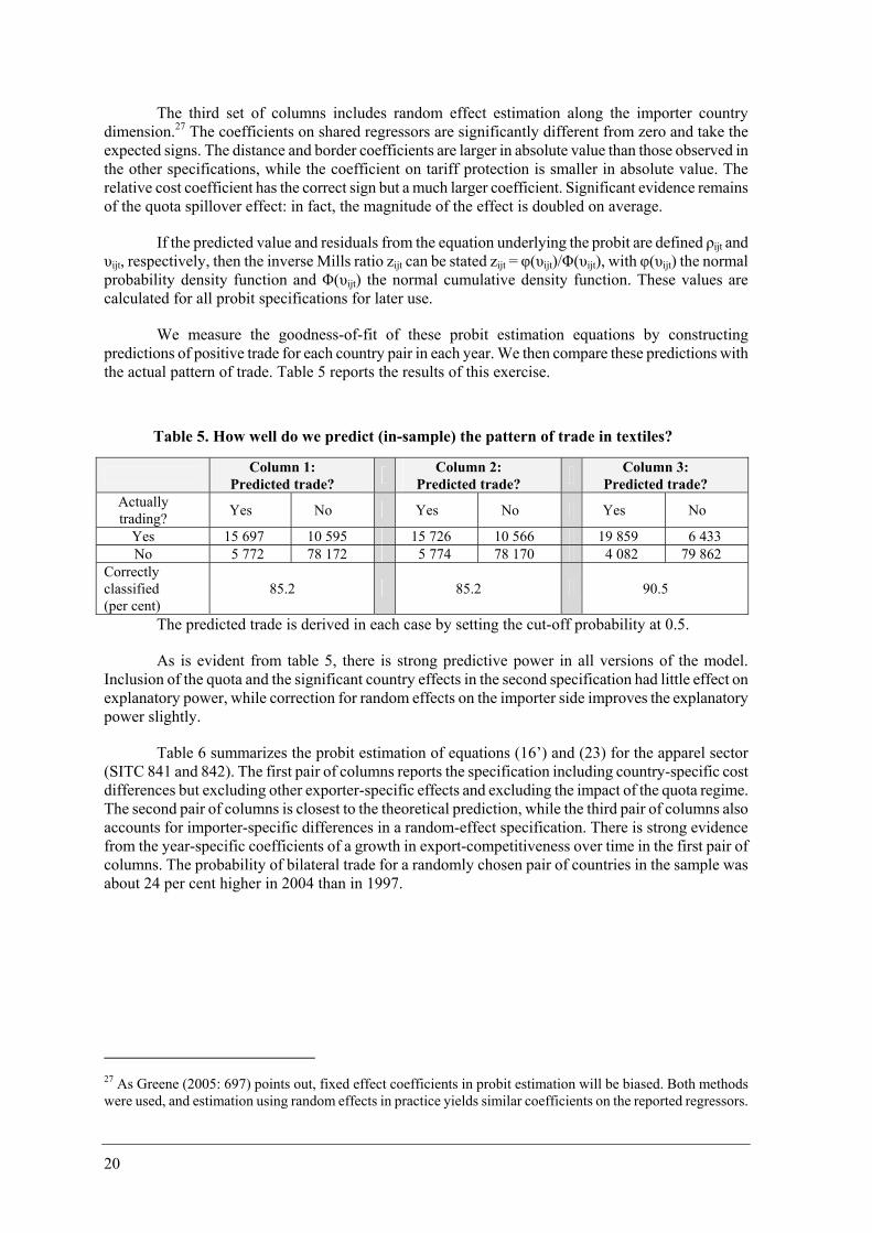
The third set of columns includes random effect estimation along the importer country dimension.27 The coefficients on shared regressors are significantly different from zero and take the expected signs. The distance and border coefficients are larger in absolute value than those observed in the other specifications, while the coefficient on tariff protection is smaller in absolute value. The relative cost coefficient has the correct sign but a much larger coefficient. Significant evidence remains of the quota spillover effect: in fact, the magnitude of the effect is doubled on average.

If the predicted value and residuals from the equation underlying the probit are defined ρijt and υijt, respectively, then the inverse Mills ratio zijt can be stated zijt = φ(υijt)/Φ(υijt), with φ(υijt) the normal probability density function and Φ(υijt) the normal cumulative density function. These values are calculated for all probit specifications for later use.

We measure the goodness-of-fit of these probit estimation equations by constructing predictions of positive trade for each country pair in each year. We then compare these predictions with the actual pattern of trade. Table 5 reports the results of this exercise.

Table 5. How well do we predict (in-sample) the pattern of trade in textiles?

Column 1: Predicted trade? Column 2:

Predicted trade? Column 3: Predicted trade?

Actually trading? Yes No Yes No Yes No

Yes 15 697 10 595 15 726 10 566 19 859 6 433 No 5 772 78 172 5 774 78 170 4 082 79 862

Correctly classified (per cent)

85.2 85.2 90.5

The predicted trade is derived in each case by setting the cut-off probability at 0.5.

As is evident from table 5, there is strong predictive power in all versions of the model. Inclusion of the quota and the significant country effects in the second specification had little effect on explanatory power, while correction for random effects on the importer side improves the explanatory power slightly.

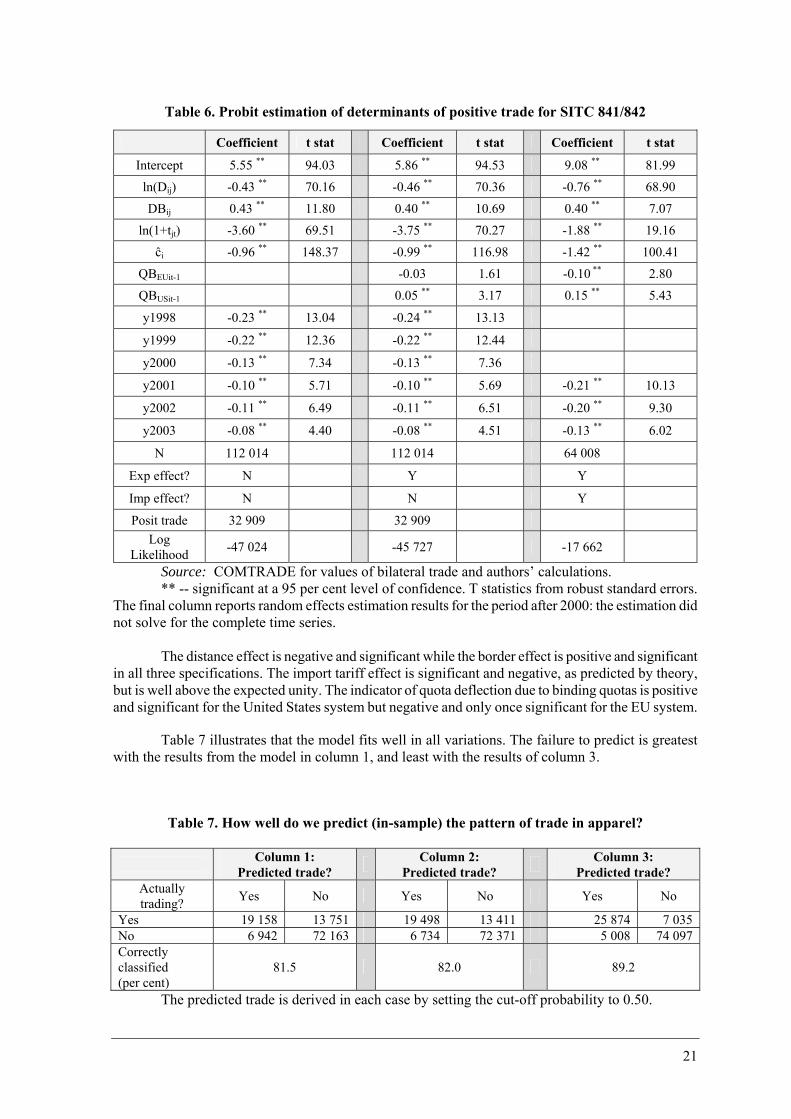
Table 6 summarizes the probit estimation of equations (16’) and (23) for the apparel sector (SITC 841 and 842). The first pair of columns reports the specification including country-specific cost differences but excluding other exporter-specific effects and excluding the impact of the quota regime. The second pair of columns is closest to the theoretical prediction, while the third pair of columns also accounts for importer-specific differences in a random-effect specification. There is strong evidence from the year-specific coefficients of a growth in export-competitiveness over time in the first pair of columns. The probability of bilateral trade for a randomly chosen pair of countries in the sample was about 24 per cent higher in 2004 than in 1997.

27 As Greene (2005: 697) points out, fixed effect coefficients in probit estimation will be biased. Both methods were used, and estimation using random effects in practice yields similar coefficients on the reported regressors.

21

Source: COMTRADE for values of bilateral trade and authors’ calculations. ** -- significant at a 95 per cent level of confidence. T statistics from robust standard errors.

The final column reports random effects estimation results for the period after 2000: the estimation did not solve for the complete time series.

The distance effect is negative and significant while the border effect is positive and significant

in all three specifications. The import tariff effect is significant and negative, as predicted by theory, but is well above the expected unity. The indicator of quota deflection due to binding quotas is positive and significant for the United States system but negative and only once significant for the EU system.

Table 7 illustrates that the model fits well in all variations. The failure to predict is greatest with the results from the model in column 1, and least with the results of column 3.

Table 7. How well do we predict (in-sample) the pattern of trade in apparel?

Column 1: Predicted trade? Column 2:

Predicted trade? Column 3: Predicted trade?

Actually trading? Yes No Yes No Yes No

Yes 19 158 13 751 19 498 13 411 25 874 7 035 No 6 942 72 163 6 734 72 371 5 008 74 097 Correctly classified (per cent)

81.5 82.0 89.2

The predicted trade is derived in each case by setting the cut-off probability to 0.50.

Table 6. Probit estimation of determinants of positive trade for SITC 841/842

Coefficient t stat Coefficient t stat Coefficient t stat

Intercept 5.55 ** 94.03 5.86 ** 94.53 9.08 ** 81.99 ln(Dij) -0.43 ** 70.16 -0.46 ** 70.36 -0.76 ** 68.90 DBij 0.43 ** 11.80 0.40 ** 10.69 0.40 ** 7.07

ln(1+tjt) -3.60 ** 69.51 -3.75 ** 70.27 -1.88 ** 19.16 ĉi -0.96 ** 148.37 -0.99 ** 116.98 -1.42 ** 100.41

QBEUit-1 -0.03 1.61 -0.10 ** 2.80

QBUSit-1 0.05 ** 3.17 0.15 ** 5.43

y1998 -0.23 ** 13.04 -0.24 ** 13.13

y1999 -0.22 ** 12.36 -0.22 ** 12.44

y2000 -0.13 ** 7.34 -0.13 ** 7.36

y2001 -0.10 ** 5.71 -0.10 ** 5.69 -0.21 ** 10.13

y2002 -0.11 ** 6.49 -0.11 ** 6.51 -0.20 ** 9.30

y2003 -0.08 ** 4.40 -0.08 ** 4.51 -0.13 ** 6.02

N 112 014 112 014 64 008

Exp effect? N Y Y

Imp effect? N N Y

Posit trade 32 909 32 909 Log

Likelihood -47 024 -45 727 -17 662

22

C. Estimating the value of bilateral trade

As theory predicts, we estimate the equation (28) reproduced below to define the determinants of the value of bilateral trade.

mijt = ωo + ω1 yjt-1 + ω2 ljt-1 + ω3 tijt + ω4 ĉi + Σt ω5t Ht + ln{exp[ω6 ρijt]-1} +

ω7 QEUi97 + ω8 QUSi97 + ω9 QNEUi97 + ω10 QNUSi97 + ω11 QBEEUit-1 + ω11 QBUUSit-1 +

ω12 QBNEUit-1 + ω13 QBNUSit-1 + Σj ω14jHj + η zijt + eijt (28)

Table 8 reports the results of this estimation for textiles. The first pair of columns is presented for comparison. It is a typical gravity model equation estimated over country pairs with non-zero imports, with inclusion of an inverse Mills ratio zij (with coefficient η) to control for countries’ selection bias. The second pair of columns reports the results from a version of the gravity equation that includes year-specific dummy variables. The third pair of columns is a modification of the estimation equation to include the exporter-specific cost differences and exclude the exporter GDP and population. The fourth pair of columns provides a complete estimate of equation (28), with separate controls for selection into imports, for exporter cost differentials and for point estimate μ of the parameter from the underlying distribution of suppliers.

Table 8. Estimation results for textiles (SITC 652)

Gravity models Theoretical specification

Intercept 10.08 ** 17.51 9.90 ** 17.17 7.40 ** 15.90 1.01 0.38 ln(Yit-1) -0.27 ** 9.10 -0.26 ** 8.67 ln(Yjt-1) 0.67 ** 38.50 0.67 ** 38.42 0.70 ** 40.52 0.71 ** 40.69 ln(Lit-1) 0.02 1.23 0.03 * 1.81 ln(Ljt-1) 0.59 ** 68.67 0.59 ** 69.11 0.60 ** 71.59 0.59 ** 70.77 ln(Dij) -1.46 ** 48.66 -1.44 ** 47.96 -1.51 ** 45.68 -0.83 ** 7.72

ln(1+tjt) -1.48 ** 7.79 -1.63 ** 8.53 -1.80 ** 9.48 -1.33 ** 6.61 ĉi -2.26 ** 39.53 -2.22 ** 38.72 -2.09 ** 11.42 -1.05 1.36 η 0.24 ** 3.76 0.20 ** 3.16 0.21 ** 3.02 0.29 ** 4.05

QEEUi97 -0.01 0.15 -0.01 0.21 0.29 0.44 0.35 ** 2.71 QUUSi97 0.59 ** 2.12 0.59 ** 2.12 0.49 1.43 QNEUi97 -0.20 ** 4.40 -0.18 ** 4.04 0.07 0.10 0.21 * 1.68 QNUSi97 0.03 0.70 0.05 1.09 -0.51 * 1.72 -0.06 0.33

QBEEUit-1 0.07 0.70 0.05 0.53 -0.08 0.72 -0.21 * 1.73 QBUUSit-1 2.77 ** 9.23 2.74 ** 9.21 2.47 ** 7.50 2.38 ** 7.20 QBNEUit-1 0.19 ** 0.93 0.18 ** 3.03 0.12 1.25 0.02 0.34 QBNUSit-1 0.27 ** 4.77 0.24 ** 4.25 -0.05 0.57 -0.14 1.54

y1998 -0.10 ** 2.04 -0.11 ** 2.30 0.51 ** 9.91 y1999 -0.22 ** 4.41 -0.24 ** 5.03 0.38 ** 7.62 y2000 -0.28 ** 5.52 -0.32 ** 6.49 0.22 ** 4.51 y2001 -0.32 ** 6.36 -0.37 ** 7.53 0.12 ** 2.49 y2002 -0.34 ** 6.56 -0.39 ** 7.89 0.08 * 1.69 y2003 -0.36 ** 6.93 -0.44 ** 8.72 0.04 0.89 μ 0.74 ** 6.63

Exp effect No No Yes Yes R2 0.44 0.45 0.50 0.50 N 26 142 26 142 26 142 26 142

Source: COMTRADE for values of bilateral trade, Penn World Tables for population and GDP, and authors’ calculations.

** -- significant at a 95 per cent level of confidence, robust standard errors.

23

The coefficient estimates are similar across specifications, and so we focus on the last pair of columns. The coefficients on year-specific dummy variables indicate a significant tendency for the mean value of bilateral imports to fall throughout the sample period – quite sharply in the period until 2000, and then slightly thereafter.28 The coefficient on the tariff variable is both negative and significantly different from zero, as predicted by theory. The estimate of η is significant and positive, indicating the importance of controlling for selection bias.29 The correction of supplier-level heterogeneity, μ = 0.74, is positive and significant; it implies an underlying distribution of firms with greater density at higher marginal costs and lower density of the low cost firms. The significant value indicates the importance of controlling for the heterogeneity of suppliers, as different values of ρijt imply different percentages of foreign firms competitive in the home market. The importer variables took the expected sign and similar magnitudes in each version.30 The cost/quality ratio ĉi is included as a proxy for quality. As quality rises, its value will fall – thus the negative coefficient is expected. It is not significantly different from zero in this specification.31

The effects of the ATC quota on the mean value of bilateral trade are investigated in two parts in this estimation. The four explanatory variables in the quota limit (QEEUi97, QUUSi97, QNEUi97, QNUSi97) measure whether quota limits are correlated with increased value of exports on average into the quota-setting country (QEEUi97, QUUSi97) or with increased value of exports to third-country importers (QNEUi97, QNUSi97) – i.e. trade deflection. We expect the coefficients of QEEUi97 and QUUSi97 to be positive – countries with quota limits are countries with above average exports to the United States or the EU.32 The coefficients of QNEUi97 and QNUSi97 will be positive for trade deflection: there is significant evidence of that for the EU quotas, and insignificant evidence against that for the United States quotas. The next four coefficients measure the additional effect of a binding quota (QBEEUit-1, QBUUSit-1, QBNEUit-1, QBNUSit-1). The own effect for United States quotas is positive and significant (2.38), while the own effect of binding EU quotas is negative and significant (-0.21). There is no evidence of trade deflection in the outside effects terms: that for the EU is positive and insignificant (0.02), while that for the United States is negative and insignificant (-0.14).33

Tables 9 and 10 report estimation results for apparel, with table 9 building up to the form of (28) and table 10 adding potentially important linkages between textile and apparel producers to each specification of table 9. Specification (1) is a gravity-like estimating equation excluding both exporter-specific cost heterogeneity and year-specific effects. Specification (2) introduces year-specific effects. Specification (3) excludes exporter GDP and population as explanatory variables while introducing exporter-cost heterogeneity. Specification (4) is closest to equation (28), with both cross-country exporter cost heterogeneity and the impact of supplier heterogeneity within countries.

28 Note the asymmetry with the pattern of trade reported earlier: each country was found to export to significantly more import destinations over time. 29 In this case, the sign of the coefficient for the inverse Mills ratio changes with the introduction of the plant distribution effects. We will be investigating the implications of this reversal carefully in future work. 30 The theory predicted that the shipping cost variables (distance and propinquity) should not enter separately. Our original specification excluded them, but we found that distance entered with a significant and negative coefficient. As a result, we retained that explanatory variable in the specifications reported here. 31 As a check of ĉi as a proxy for quality, we created a measure of unit values in cotton cloth imports into the United States. If unit values are a measure of quality, then the inverse of ĉi should be positively correlated with the unit value. We found a positive and significant correlation of 0.33 for a subsample of 105 countries in 2004. These results are available on request. 32 Note that this effect is calculated simultaneously with fixed effects for each exporter. A large exporter to all countries will have a large fixed effect; the effect of the quota measured here is in addition to that. 33 Note that this effect is calculated simultaneously with fixed effects for each exporter. A large exporter to all countries will have a large fixed effect; the effect of the quota measured here is in addition to that.

24

Table 9. Estimation results for apparel (SITC 841/842)

Equation (1) (2) (3) (4) Intercept -2.99 ** 7.90 -3.17 ** 8.35 -5.75 * 1.71 -4.68 * 1.72 ln(Yit-1) -0.10 ** 5.02 -0.09 ** 4.63 ln(Yjt-1) 1.33 ** 62.88 1.32 ** 62.13 1.45 ** 69.04 1.27 ** 60.82 ln(Lit-1) 0.18 ** 14.98 0.18 ** 15.23 ln(Ljt-1) 0.50 ** 59.69 0.50 ** 59.66 0.54 ** 66.11 0.48 ** 59.86 ln(Dij) -1.06 ** 68.18 -1.05 ** 67.29 -1.10 ** 67.93 -0.94 ** 57.27 ĉi -1.58 ** 44.28 -1.55 ** 43.40 -0.48 0.46 -2.43 ** 2.84

η -0.70 ** 16.34 -0.73 ** 17.04 -0.52 ** 11.78 2.51 ** 24.07 ln(1+tjt) -1.77 ** 11.70 -1.86 ** 12.27 -1.99 ** 13.54 -2.18 ** 15.16 QEEUj97 1.36 ** 22.45 1.35 ** 22.27 1.22 ** 2.04 y QUUSj97 3.48 ** 15.43 3.47 ** 15.35 4.51 ** 2.29 y QNEUj97 0.22 ** 6.34 0.23 ** 6.44 0.12 0.21 y QNUSj97 -0.24 ** 6.05 -0.23 ** 5.80 0.95 0.49 y

QBEEUjt-1 0.70 ** 8.57 0.72 ** 8.73 0.60 ** 5.22 0.62 ** 5.50 QBUUSjt-1 1.80 ** 6.50 1.78 ** 6.35 1.67 ** 6.22 1.75 ** 6.83 QBNEUjt-1 -0.05 1.10 -0.04 0.85 -0.18 * 1.87 -0.19 ** 2.07 QBNUSjt-1 0.26 ** 5.41 0.24 ** 4.99 0.09 1.26 0.06 0.92

y1998 0.39 ** 8.69 0.21 ** 4.56 0.45 ** 10.63 y1999 0.27 ** 6.09 0.09** 2.04 0.33 ** 7.91 y2000 0.06 1.31 -0.04 1.06 0.09 ** 2.23 y2001 0.02 0.48 -0.08 * 1.85 0.04 0.91 y2002 0.08 * 1.79 -0.04 0.89 0.06 1.59 y2003 0.10 ** 2.38 0.03 0.74 0.11 ** 2.62 μ 6.81 ** 34.34

Exporter dummy No No Yes Yes N 32 698 32 698 32 698 32 698 R2 0.54 0.54 0.60 0.62

Source: COMTRADE for values of bilateral trade, World Development Indicators for population

and GDP, and authors’ calculations. ** -- significant at a 95 per cent level of confidence, robust standard errors. y - incredibly high

values

Consider specification (4) in table 9. The year-specific effects are uniformly positive, indicating reduction in mean value of exports from 1997 on, but these effects are concentrated in the period 1997–2001. The importer GDP, importer population and distance variables all have significant coefficients of the expected sign. The importer tariff variable also takes the expected negative sign and is significantly different from zero. The inverse Mills ratio correction for selection bias has coefficient η=2.51 and is significantly different from zero. The effect μ of supplier heterogeneity is at 6.81 both large and significant: it indicates a distribution of suppliers within each country highly skewed towards higher cost production.

The ATC system of quotas is introduced in two parts, as in the previous section. The exports of quota-limited or quota-bound country i to quota-imposing countries are significantly larger in each case than exports by non-quota-limited or -bound exporters: these effects are maintained even when exporter fixed effects are introduced. There is insignificant evidence of trade deflection by binding

25

United States quotas, as illustrated in the coefficient on QBNUSit. The coefficient on QBNEUit is negative and significant, and tells an interesting story – countries with binding EU quotas in apparel export significantly less to non-EU countries on average. These are truly export platforms, and platforms only for the EU market.

Table 10. Estimation results for apparel (SITC 841/842) accounting

for links to textiles (SITC 652)

Equation (1) (2) (3) (4) Intercept -7.78 ** 20.61 -7.90 ** 20.93 -5.27 16.08 y ln(Yit-1) -0.11 ** 4.30 -0.10 ** 4.05 ln(Yjt-1) 1.06 ** 41.79 1.05 ** 41.49 1.23 ** 29.34 1.18 ** 48.15 ln(Lit-1) 0.14 ** 9.12 0.14 ** 9.23 ln(Ljt-1) 0.35 ** 25.16 0.35 ** 25.25 0.40 ** 29.34 0.48 ** 36.50 ln(Dij) -0.17 ** 5.69 -0.16 ** 5.61 -0.56 * 19.72 0.24 ** 2.27 ĉi

-1.18 ** 30.83 -11.03 ** 79.18

η -1.17 ** 28.20 -1.19 ** 28.80 -0.62 ** 14.26 2.57 ** 23.99 ln(1+tjt) -1.11 ** 7.17 -1.26 ** 8.08 -1.62 ** 10.50 -1.63 ** 11.05 QEEUj97 1.42 ** 21.83 1.41 ** 21.64 1.09 ** 14.86 y QUUSj97 3.61 ** 18.19 3.61 ** 18.02 4.16 ** 20.20 y QNEUj97 0.6 ** 7.19 0.27 ** 7.42 -0.06 1.23 y QNUSj97 -0.52 ** 12.85 -0.50 ** 12.22 0.12 ** 2.20 y

QBEEUjt-1 0.80 ** 9.00 0.81 ** 9.16 0.68 ** 7.64 0.58 ** 5.12 QBUUSjt-1 1.70 ** 7.52 1.65 ** 7.19 1.40 ** 6.04 1.26 ** 5.56 QBNEUjt-1 -0.01 0.11 0.01 0.10 -0.04 0.68 -0.18 ** 1.96 QBNUSjt-1 0.51 ** 10.32 0.46 ** 9.40 0.31 ** 6.21 0.03 0.40

y1998 0.48 ** 10.38 0.40 ** 8.76 0.53 ** 12.24 y1999 0.35 ** 7.53 0.26 ** 5.82 0.37 ** 8.82 y2000 0.11 ** 2.32 0.06 1.35 0.13 ** 3.06 y2001 0.03 0.67 -0.00 0.05 0.02 0.51 y2002 0.10 ** 2.31 0.06 1.31 0.06 1.52 y2003 0.10 ** 2.29 0.09 ** 1.96 0.09 ** 2.13 μ 6.80 ** 33.53 ŝijt 0.73 ** 30.43 0.72 ** 30.08 0.42 ** 19.64 1.13 ** 10.23 ŝjit 0.13 ** 6.94 0.13 ** 6.91 0.15 ** 7.96 0.13 ** 7.20

Exporter dummy No No Yes Yes N 31 905 31 905 31 905 31 905 R2 0.53 0.53 0.55 0.62

Source: COMTRADE for values of bilateral trade, World Development Indicators for population

and GDP, and authors’ calculations. ** -- significant at a 95 per cent level of confidence, robust standard errors. y – unreasonably high

values

26

VI.  Linking the two sectors 

The preceding analysis was undertaken with the assumption that the textiles and apparel industries were independent. In fact, they are closely linked along two dimensions. First is the technological dimension: because the two industries developed together and are two stages in a final product, it is to be expected that countries with a comparative advantage in the production of textiles will (other things equal) have an existing production of apparel. Second is the dimension of regional integration: if a country has comparative advantage in the production of textiles, it will look for regional partners to process the textiles into apparel for re-export to the country of origin of the textiles. Each of these is investigated in turn in this section.

Given that the textiles sector is the upstream sector in this linkage, analysis of that sector is unchanged. The probit estimation for textiles is used to create two fitted values in predicting trade flows: ŝijt is the prediction that country i will export textiles to country j, while ŝjit is the prediction that country i will import textiles from country j. The ŝijt variable will pick up the common cost advantage of a textiles producer (or economies of scope): if a country has a natural comparative advantage in both, or there are economies of scope, then positive ŝijt will be correlated positively with export of apparel. The coefficient of ŝjit will take a positive value when there is evidence that textiles exporters more often sell to importers using the textiles for offshore assembly and re-import of apparel to the textile-exporting country.

The specifications in table 10 extend the structure of table 9 to include the variables ŝijt and ŝjit. For countries predicted to be textile exporters to country j in period t, the value of apparel exports to country j is also significantly more – this is consistent either with an argument of common comparative advantage in the two sectors or in an argument of economies of scope in internalizing textiles and apparel production within the same supplier. An increase in the probability of textiles export from country i to country j tends to increase the mean value of apparel exports from i to j by 1.13 per cent in specification (4). An increase in the probability of textiles export from country i to country j also increases significantly the mean value of apparel exports from j to i, by a nearly constant 0.13 per cent in the four specifications. This is an indicator of “offshoring”. Specification (4) is the closest to the theoretical specification. Importer GDP and population effects are significant and take the expected sign. Importer tariff also has a strongly negative effect on the mean value of imports. The inverse Mills ratio takes the coefficient η=2.57, similar to that observed in the estimations reported in table 9. The quota spillover effects are also similar to those reported above. The supplier heterogeneity effect μ = 6.80 is significantly different from zero and similar to that of table 9.

When we consider the coefficients linking textiles and apparel, we see large jumps in the “economies of scope” effect but stability of the offshoring effect. For the offshoring effect proxied by ŝjit, the elasticity falls in the narrow range (0.13–0.15). For the economies of scope effect proxied by ŝijt, the elasticity falls in the wider range (0.42–1.13). Both effects are always significantly different from zero.

27

VII. Predicting the effect of removing quota restrictions 

Since 2005 marks the end of the quota system, theory predicts that the pattern of trade in these two categories will become more focused: fewer countries will export to those countries formerly under quota (less trade diversion) and those exporters serving the formerly quota-restrained countries will export to fewer other countries (less trade deflection). This is not immediately evident in the data, as table 11 illustrates.

Table 11. Proportion of non-zero bilateral trade pairs in sample (128 countries)

Year Textiles (652) Apparel (841/842)

1997 21.8 25.0

1998 22.3 25.8

1999 22.7 26.1

2000 22.9 28.2

2001 23.4 29.1

2002 23.5 29.7

2003 23.8 31.0

2004 23.7 33.1

2005 24.9 35.7

For these 128 countries, there are 146,304 observations of bilateral imports over the nine-year sample. If the share of bilateral observations with non-zero trade is calculated for each year, it is evident that in both textiles and apparel there has been a diversification in trading patterns. The share of possible bilateral pairs with non-zero textiles imports was 21.8 per cent in 1997; by 2004 it was 23.7 per cent. In apparel, a similar calculation yields 25 per cent in 1997 and 33.1 per cent in 2004. This increased share is consistent with steadily increasing trade diversion and trade deflection from an increasingly binding system of quotas.

This explanation is less compelling, though, for 2005. With the removal of quota restrictions, other things equal, we predict a fall in this percentage. Instead, there is a jump in both shares larger than observed in previous years. These shares are unconditional means, and as such do not reflect the impact of other possible determinants. To address this question properly, we undertake a comparative static exercise based upon the estimation results of the previous sections.

First we examine the estimated impact of quota restrictions from the data panel for the quota-driven period 1998–2004. The coefficients are derived in the earlier section and are reproduced in table 12. The first two columns represent the effect of the quota on the observed pattern of trade, while the last two columns represent the effect of the quota on the mean value of imports given that trade occurs. These coefficients are taken from the theoretically consistent regressions (right-hand column) of each table.

28

Table 12. The implications of the quota regime for trade

Apparel Probit Structural Estimation Coefficient T statistic Coefficient T statistic

QEUj97

QEEUj97 1.22 ** 2.04 QUUSj97 4.51 ** 2.29 QUSj97 QNEUj97 0.12 0.21 QNUSj97 0.95 0.49 QBEUjt-1 -0.10 ** 2.80 QBEEUjt-1 0.60 ** 5.22 QBUUSjt-1 1.67 ** 6.22 QBUSjt-1 0.15 ** 5.43 QBNEUjt-1 -0.18 * 1.87 QBNUSjt-1 0.09 1.26 Textiles Coefficient T statistic Coefficient T statistic QEUj97

QEEUj97 0.35 ** 2.71 QUUSj97 0.49 1.43 QUSj97

QNEUj97 0.21 * 1.68 QNUSj97 -0.06 0.33 QBEUjt-1 -0.10 ** 5.30 QBEEUjt-1 -0.21 * 1.73 QBUUSjt-1 2.38 ** 7.20 QBUSjt-1 -0.14 ** 4.40 QBNEUjt-1 0.02 0.34 QBNUSjt-1 -0.14 1.54

These coefficients are reproduced from tables 3, 6, 8 and 9.

The observed pattern of trade in textiles is not significantly affected by the existence of quota limits, but there is a significant effect of binding quotas on the pattern of trade.34 Theory suggests that these coefficients will be positive – a quota limit or binding quota will encourage the exporter to develop new export markets. The econometric results in only one of four cases support that conclusion. In textiles, the country with binding quota, whether of the United States or the EU, will – other things equal – have a significant lower probability to export to the average importer. In apparel, a binding quota in the United States has the expected effect of increasing the probability of exporting to an average importer, while a binding quota in the EU has a significant effect in the opposite direction.

The effects of quota limits on the average value of exports by the country under quota can be broken into the impact on the quota-setting country and on other countries. The quota limits, whether by United States or the EU, are associated with significantly large mean value exports to the quota-setting country, other things equal. The effect on the mean export value to other countries is predominantly negative. Consider the example of the United States: quota limits on an apparel exporter are associated with significantly larger imports by the United States from that country (3.38) but a minimal and insignificant effect on imports by other countries (-0.01). Quota limits on a textiles exporter are also associated with a significantly positive change in mean value of United States imports from that exporter (0.49), but a negative and insignificant effect on mean value of exports of that country to non-United States importers (-0.06). The causality here should probably be reversed –

34 The coefficients on quota limits are not reported, just as in the preceding tables, but augmented probits including those quota limits led to insignificant coefficients on those variables.

29

exporting countries are given quota limits when they demonstrate the ability to export large amounts to the United States (or the EU). Binding quotas have a significant additional effect on quota limits for the quota-setting country: for the United States, 1.52 and 2.38 for apparel and textiles respectively. The effect of these binding quotas on the mean value of exports to non-quota-setting countries is generally insignificant for both EU and United States quotas.

For a second investigation of the impact of quotas, we use out-of-sample forecasting to check actual against predicted patterns of trade. We begin from the quota-distorted equilibrium of 1998–2004 as summarized in the probit regression results of tables 3 and 6 and the non-linear regression results of tables 8 and 9. We then use these results to forecast the trade pattern and trade volume in 2005. Table 13 summarizes our results for the trade pattern.

The χ2 (1) statistic represents the difference between the given distribution and a distribution with equally distributed errors in prediction.

These out-of-sample forecasts were calibrated on the 1998–2004 data, and in this table the estimated probability used to separate predicted trade from no predicted trade was chosen to ensure equal numbers of type 1 and type 2 errors (Actual: no; predicted: yes – or Actual: yes; predicted: no) in that sample. As is evident in table 13, the model’s predictions for 2005 are significantly skewed toward (Actual: yes; predicted: no) errors both for textiles and for apparel: we have observed greater numbers of bilateral trading combinations. Just as is evident in table 11, this exercise indicates that 2005 was a period of diversifying trade unpredicted by the simple model of Vinerian trade creation. The hypothesis that removal of quotas will lead to greater trade focus – i.e. less trade diversion and less trade deflection – does not hold in aggregate for 2005, even when controlling for other factors that might affect trade patterns.

Tables 14 and 15 compare bilateral mean export value and number of export markets on average in 1997–2004 to 2005 for each exporter. The Vinerian prediction was to observe the quota-bound countries in the lower left-hand corner: increased mean export value and reduced number of export markets. In table 14, the results for textiles trade indicate that other than China, this is not the case – that category is dominated by the developed countries in Europe, Japan and the United States. The combination of reduced mean export value and increased number of export markets is the most often observed and includes the largest group of developing countries. Table 15 illustrates a similar pattern for bilateral trade in apparel.35

The country acronyms in bold in these two tables are the countries subject to binding quotas in 2004. The pattern of these is suggestive – a binding quota in 2004 is associated with a reduced number of export markets in 2005, as the Vinerian hypothesis suggests.

35 A large number of countries fall into the “missing data” category. For these, the 2005 figures on GDP and population were not available to create predicted trade values for 2005. Once the data set is updated, we will be able to move these countries into the left-hand quadrants of the tables. For comparison, tables A4 and A5 in appendix 3 provide the complete unconditional mean assignments of countries to these categories.

Table 13. Out-of-sample forecasts for the trade pattern in 2005

Textiles: predicted trade? Apparel:

predicted trade? Bilateral pair actually trading? Yes No Yes No

Yes 3 071 963 4 458 1 323 No 715 10 999 873 9 348 Correctly classified (per cent) 89.3 86.3 χ2 (1) test: significant imbalance 36.6 ** 92.2 **

30

x – indicates that the actual and predicted number of export markets was the same. Country acronyms in bold are those with binding quotas from either the EU or the United States (or both) in 2004.

x – indicates that the actual and predicted number of export markets was the same. Country acronyms in bold are those with binding quotas from either the EU or the United States (or both) in 2004.

Table 14. Actual versus predicted trade in textiles in 2005

Increased mean export value

Reduced mean export value

Missing data on mean export value in 2005

Increased number of export markets

ESP, FRA, TUR PAKx

ARG, AUS, BFA, BGR, BLZ, CHL, CRI, CZE, ECU, EST, FIN, GAB, GRC, IDN, ISL, LTU, MDA, MDG, MLI, MUS, MWI, NER, NIC, NZL, PHL, POL, SVN, SWE, TGO, TUN, URY CYPx, GEOx, HNDx

AZE, BDI, BEN, BGD, BHR, BOL, CMR, DMA, DZA, EGY, GHA, GTM, GUY, JOR, KAZ, KEN, LBN, LKA, MAR, MNG, MOZ, NPL, OMN, PAN, PRY, QAT, SDN, SEN, SLV, SYC, SYR, THA, TTO, TZA, UGA, UKR, VCT, VNM, YEM, ZMB

Reduced number of export markets

AUT, ALB, CHN, DEU, GBR, ITA, JPN, NLD, PRT, USA

CAN, DNK, HKG, HRV, HUN, IRL, ISR, KOR, MEX, MLT, SGP, SVK, TWN, VEN, ZAF

BLR, BRA, CIV, COL, IND, IRN, JAM, KGZ, LVA, MRT, MYS, RUS, SAU

Table 15. Actual versus predicted trade in apparel in 2005

Increased mean export value

Reduced mean export value

Missing values on 2005 export value

Increased number of export markets

BGR, ESP, GAB, GEO, MLI, NLD, PAK, PHL, POL, SVK, SWE, TUN, TUR CZE x

ARG, AUS, AUT, BFA, BLZ, CHL, CRI, FIN, GRC, HND, ISL, ISR, JPN, LTU, MDG, MEX, MUS, MWI, NIC, NZL, TGO, URY, VEN IRL x, NERx

ARM, AZE, BEN, BGD, BHR, BOL, BRA, CAF, CIV, CMR, COL, DMA, DZA, EGY, GHA, GTM, GUY, IRN, JAM, JOR, KAZ, KEN, KGZ, KHM, KNA, LBN, LCA, LKA, LVA, MAR, MNG, MOZ, MRT, MYS, NPL, OMN, PER, QAT, RUS, SAU, SDN, SEN, SLV, SYC, SYR, TTO, TZA, UGA, UKR, VCT, VNM, YEM, ZMB

Reduced number of export markets

CAN, CHN, DEU, DNK, FRA, GBR, HKG, HRV, IDN, ITA, MDA, MLT, PRT, SVN

ALB, CYP, ECU, EST, HUN, KOR, MDV, NOR, SGP, TWN, USA, ZAF

THA, IND, PAN, BLR, PRY, GRD

31

The majority of countries, though, are associated with an increased number of export markets. These will be the countries finding fewer purchasers in the United States and EU markets post-quota; their producers then adjust by selling less to a greater number of other importers.

Comparing actual and predicted for 2005, as done here, leaves open three possibilities for the source of the change. First, the removal of the quota system may have triggered the effect. Second, there could have been a change to the common costs of or benefits from bilateral trade that led to a change in “normal” trade. Third, there could have been country-specific idiosyncratic effects that caused the divergence. The analysis preceding this combined these three possibilities. We examine the evidence of the second effect by measuring the change in coefficients of the probit and regression equations when 1998–2004 and 2005 are compared. Table 16 reports these results.

The coefficients reported in the “1998–2004” columns of table 16 are the coefficients on the explanatory variables estimated in the 1998–2004 analysis reported earlier. The “2005” columns represent the change in the coefficient when the same analysis is done for 2005 alone. (For example, the coefficient on ln(Dij) for textiles in 1998–2004 was -0.92, while the coefficient in 2005 is -0.87. The difference for 2005 is reported. The T statistic tests whether the difference 0.05 is significantly different from zero.) Significant differences indicate a fundamental change in the “normal” pattern and value of trade as defined in earlier sections. The significant coefficients on distance (Dij) and contiguity (DBij) in the pattern of trade indicate that the transport costs of trade in textiles and apparel have declined significantly in 2005. The significant negative change in the coefficient on average tariff (1+tjt) indicates that tariffs took on a larger discouraging effect on establishing trade in 2005. In examining the coefficients from the “value of trade” equations, we observe that the economic size of the importing country (ln(Yjt-1), ln(Ljt-1)) played a significantly larger role in increasing the mean value of trade in 2005. The quality of the export goods (ĉi) also became a larger determinant of the value of trade – there was a “flight to quality” in 2005 when countries were no longer constrained by quotas.

Table 16. The change in “normal” trade relations in 2005

Textiles Apparel

1998–2004 2005 2005 T-stat 1998–2004 2005 2005

T-stat Pattern of

trade

ln(Dij) -0.92 ** 0.05 * 1.91 -0.81 ** 0.09 ** 3.92

DBij 0.58 ** 0.30 ** 2.10 0.40 ** 0.18 1.13

ln(1+tjt) 0.19 -0.91 ** 4.03 0.44 ** -0.40 ** 2.42

ĉi -1.45 ** -0.01 0.36 -1.47 ** 0.05 ** 2.39 Value of

trade

ln(Yjt-1) 0.71 ** 0.06 0.71 1.47 ** 0.25 ** 6.64

ln(Ljt-1) 0.60 ** 0.21 ** 6.81 0.54 ** 0.17 ** 6.52

ln(Dij) -1.43 ** -0.21 ** 3.85 -1.08 ** -0.45 ** 10.76

ln(1+tjt) -1.77 ** -1.00 0.92 -1.95 ** 2.56 ** 4.31

ĉi -2.36 ** -0.31 ** 2.10 -0.49 -0.44 ** 6.52

Source: authors’ calculations ** - significant at a 95 per cent level of confidence * - significant at a 90 per cent level of confidence

32

VIII. Conclusions and extensions 

The global story of the removal of quotas on textiles and apparel has been told in large part from the perspective of the quota-setting countries, and in particular the United States and the members of the EU. This paper nests that perspective within the global fabric of trade. The removal of the ATC quotas in 2005 served as a shock to which all trading countries must adjust – not just consumers in the United States and the EU. The conclusion of this paper supports the Vinerian trade creation story, but with a twist. While the countries presumed to be comparative advantage exporters of textiles and apparel exhibit the expected increased exports to the quota-removing importers, the other exporters whose market has been reduced in the United States and the EU have expanded their exports to larger numbers of smaller importers than they served during the quota period.

The model presented here proves to be effective in capturing both the pattern and value of international trade in textiles and apparel, and may be useful in other industry-level trade studies. It introduces a number of improvements over the typical gravity equation or computable general equilibrium (CGE) model. First, it identifies the comparative cost advantage of exporting countries by looking across importers, rather than simply at the United States or the European market. Second, it incorporates the heterogeneity of suppliers within the exporting country; this proves to be an important factor in explaining the variation of export success by the same country across trading partners. Third, it introduces the impact of the ATC system of bilateral quotas imposed by the United States, the EU and Canada during this period. Fourth, it endogenizes the export platform explanation for offshoring.

The heterogeneity of suppliers within an exporting economy is advanced in Melitz (2003) and Helpman et al. (2008) as a useful way to consider the incremental nature of exporter response to export incentives. This proves its worth in the present analysis. The pattern of trade provides us with an insight into that heterogeneity that can be exploited and then applied to distinguish the impact of the quota regime.

The deflection effect of quotas on other importers is evident in the data. First, quotas in the United States and the EU are associated with exports to more non-quota destinations, even after controlling for importer size, distance, tariffs and other features of the economies. Second, there is evidence that binding apparel quotas in the United States are associated with increased apparel exports by those constrained exporters in other countries.

There is strong support in the data for the export platform argument. If country j exports textiles to country k, then the value of apparel exports from k to j is significantly increased.

Use of the model for out-of-sample forecasts of textiles and apparel exports in 2005 suggests a reality that is more complex than the simple prediction that “China takes over the market”. The year 2005 was not characterized overall by the “focusing” of the pattern of trade suggested by the simple predictions of CGE models – there was in fact an increased diversification of trading patterns over the quota-restricted periods on average. There was also a reduction in the average trading volume of both exporters and importers during 2005, but this was a continuation of a trend evident in the data in previous years.

The technique used here has not only identified the “normal” trade pattern and mean value of trade, but has also identified countries that stand out in their success in dealing with the removal of the ATC quotas. In examining tables 14 and 15, for example, we note the success of Pakistan and Turkey in both expanding the number of importers for their textiles and apparel and expanding the mean value of shipments to those importers. It will be useful to investigate these successful countries more closely, specifically in the context of the heterogeneous supplier framework put forward by Helpman et al. (2008). This can be done through the analysis of plant-level decision-making.

33

Bibliography

Baranga T (2008). How empirically important are zero trade flows and firm-level heterogeneity when estimating gravity equations?

Bown C and Crowley M (2007). Trade deflection and trade depression. Journal of International

Economics. 72: 176–201. Brambilla I et al. (2007). China’s experience under the MultiFiber Arrangement and the Agreement on

Textiles and Clothing. NBER working paper 13346. Conway P (2007). Global implications of unraveling textiles and apparel quotas. Dean J (1990). The effects of the US MFA on small exporters. Review of Economics and Statistics.

72(1): 63–69. Dean J (1995). Market disruption and the incidence of VERs under the MFA. Review of Economics

and Statistics. 77(2): 383–388. Dixit A and Stiglitz J (1977). Monopolistic competition and optimum product diversity. American

Economic Review. 97: 297–308. EEC (2005). Annex 8, EEC Council Regulation 3030/93, as updated in EC Commission

Regulation 930/2005. Francois J et al. (1977). Impacts of textiles and clothing sectors liberalisation of price. Final report.

Kiel Institute for the World Economy. Greene W (2005). Econometric Analysis. New York, Prentice Hall. Hallak JC (2006). Product quality and the direction of trade. Journal of International Economics.

68(1): 238–265. Harrigan J and Barrows G (2006). Testing the theory of trade policy: evidence from the abrupt end of

the Multifibre Arrangement. NBER working paper 12579. Heckman J (1974). Shadow prices, market wages, and labor supply. Econometrica. 42: 679–694. Helpman E et al. (2008). Trading partners and trading volumes.Quarterly Journal of Economics,

123 (2): 441–487. Maddala G (1983). Limited Dependent and Qualitative Variables in Econometrics. Cambridge,

Cambridge University Press. Melitz M (2003). The impact of trade on intraindustry reallocations and aggregate industry

productivity. Econometrica. 71: 1695–1725. OTEXA (2003). Summary of Agreements. Viner J (1950). The Customs Union Issue. London, Carnegie Endowment for International Peace.

35

Appendix 1. Trade focus – and trade deflection 

1. Increased trade focus in apparel: increased mean value, reduced number of export markets CAN, DNK, ESP, ITA, USA BRA, CHN, HKG, HUN, IDN, IND, LKA, MAR, PHL, THA, TUR, VNM 2. Increased trade focus in textiles: increased mean value, reduced number of export markets AUT, ITA, JPN, PRT BRA, CHN, IND, PAK, TUR 3. Trade deflection after the removal of quotas: reduced mean value, but increased number of export markets In textiles: AUS, DNK, IRL, NOR, SWE ARG, AZE, BEN, BFA, BGD, BLZ, BRB, CHL, CIV, CMR, COL, CRI, CYP, CZE, DMA, DZA, ECU, EGY, GHA, GTM, GUY, HND, HRV, IRN, ISR, JAM, JOR, KAZ, KEN, LBN, LKA, LTU, MDA, MEX, MKD, MLI, MLT, MNG, MOZ, MRT, MUS, MWI, NER, NIC, NPL, OMN, PAN, PER, PRY, QAT, RUS, SAU, SDN, SEN, SGP, SLV, SVK, SVN, SYC, TGO, TTO, TUN, TZA, UGA, VCT, VEN, YEM, ZAF, ZMB In apparel: AUS, FIN, GRC, IRL, ISL, NOR, NZL, SWE ALB, ARM, AZE, BFA, BHR, BLZ, BRB, CHL, CIV, CMR, COL, CYP, DMA, DZA, ECU, EST, GEO, GHA, GRD, GTM, GUY, HND, IRN, ISR, JAM, KAZ, KEN, KGZ, KNA, LCA, LSO, MDG, MDV, MLI, MLT, MNG, MOZ, MRT, MWI, NER, NIC, OMN, PRY, QAT, RUS, SAU, SDN, SEN, SLV, SYR, TGO, TTO, TZA, URY, VCT, VEN, YEM, ZMB

36

Appendix 2. Measuring the quota system 

The quota system under the MFA and ATC agreements is described in section II. Quotas in these agreements were defined for product categories narrower than the 3-digit SITC classification used in this paper. We use a mapping rule in classifying a country subject to a quota limit or a binding quota. First, we define the set of quota categories that covered products in the 652 and 841/842 SITC classifications. Second, we defined a country as subject to a quota limit if the United States or the EU had specified a quota limit for that exporting country in any one of those categories. Third, following Dean (1990) and Dean (1995), we categorized an exporting country as subject to a binding quota if its observed quantity exported in that year was greater than 90 per cent of the quota limit. We used data provided by the OTEXA Division of the United States Department of Commerce and by the EU to calculate this percentage.

Table A1. Quota limits (and binding quotas) in 1997

United States – textiles (25/13)

EU – textiles (41/11)

United States – apparel (44/34)

EU – apparel (46/16)

ARE, BRA, CHN*, ALB, ARE, ARG, ARE*, BGD*, BHR, ALB, ARE, ARM, COL, CZE, EGY*, ARM, AZE, BGR*, BRA, CHN*, COL*, AZE, BGD, BGR, HKG*, HUN, IDN*, BLR, BRA, CHN*, CRI*, CZE, DOM*, BLR*, BRA, CHN*, IND*, LKA, KOR*, CZE*, EGY, EST, EGY*, FJI*, GTM*, CZE, EGY, EST, MAC, MUS, MYS*, GEO, HKG, HUN, HKG*, HND, HUN, GEO, HKG*, HUN, PAK*, PHL*, POL, IDN*, IND*, KAZ, IDN*, IND*, JAM*, IDN*, IND*, KAZ, ROM*, SGP, SVK, KGZ, KOR*, KSV, KEN, KOR*, KWT, KGZ, KOR*, KSV, THA*, TUR*, TWN*, LTU, LVA, MDA, LAO*, LKA*, MAC*, LKA*, LTU, LVA, URY MKD, MLT, MYS, MKD*, MMR, MUS*, MAC*, MAR, MDA, PAK*, PER, POL*, MYS*, NPL*, OMN*, MKD, MLT, MNG, ROM, SGP, SVK, PAK*, PHL*, POL*, MYS*, PAK*, PHL*, SVN, THA*, TJK QAT*, ROM*, RUS*, POL, ROM*, SGP, TKM, TUN, TWN*, SGP*, SLV*, SVK, SVK, SVN, THA*, UZB, VNM* THA*, TUR*, TWN*, TJK, TKM, TUN, UKR*, URY TWN*, UKR*, UZB, VNM*

Source: authors’ calculations.

Table A1 indicates the countries subject to quota limits in 1997 – these were the countries i designated with 1 in QEUi97 and QUSi97. Those with binding quotas in 1997 are marked with an asterisk. The totals of countries with quota limits and with binding quotas are given in parentheses at the top of each column. Note that the number of countries with quota limits is relatively small compared to the total universe of potential exporters. Note also that the percentage of countries with binding quotas is relatively high due to the aggregation performed here. In any single quota category, the number of countries subject to binding quotas will typically be closer to 10 per cent. See Conway (2007) for examples.

Tables A2 and A3 report the correlation between quota limits and binding quotas for the United States and EU in 1997. The correlation is calculated over the 79 countries for which at least one importer had established a quota limit in either cotton textiles or cotton apparel in 1997.

37

Table A2. Correlation of quota limits and binding quotas in textiles, 1997

QUS97 QBUS97 QEU97 QBEU97

QUS97 1.00 0.65 ** 0.26 ** 0.43 **

QBUS97 1.00 0.28 ** 0.51 **

QEU97 1.00 0.38 **

QBEU97 1.00

Table A3. Correlation of quota limits and binding quotas in apparel, 1997

QUS97 QBUS97 QEU97 QBEU97

QUS97 1.00 0.78 ** -0.08 0.32 **

QBUS97 1.00 0.01 0.45 **

QEU97 1.00 0.43 **

QBEU97 1.00

Source: authors’ calculations.

There is a strong positive but not perfect correlation between countries facing binding quotas from the two importers. By contrast, the set of countries facing quota limits in textiles is not so strongly positively correlated, and in apparel is not significantly correlated.

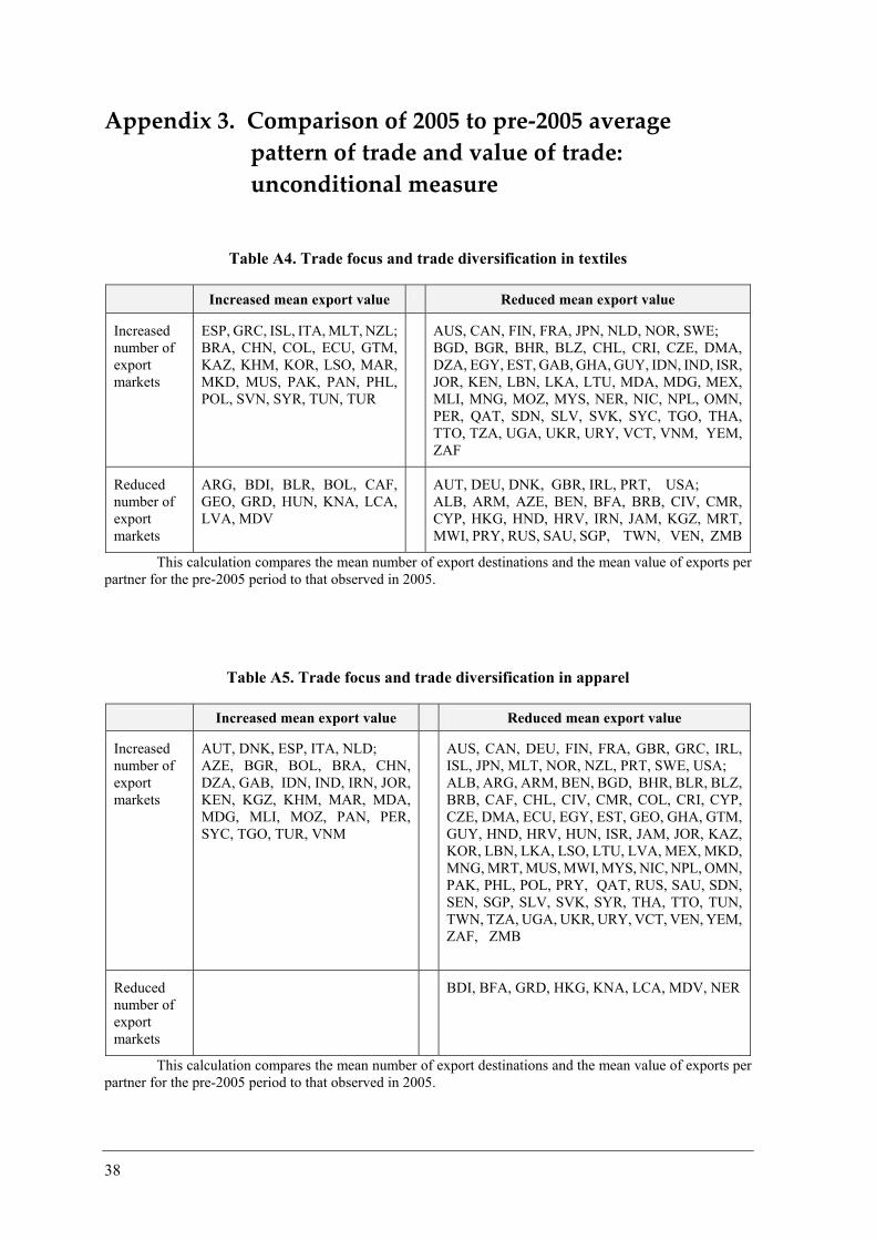
38

Appendix 3.  Comparison of 2005 to pre‐2005 average pattern of trade and value of trade: unconditional measure 

This calculation compares the mean number of export destinations and the mean value of exports per partner for the pre-2005 period to that observed in 2005.

This calculation compares the mean number of export destinations and the mean value of exports per partner for the pre-2005 period to that observed in 2005.

Table A4. Trade focus and trade diversification in textiles

Increased mean export value Reduced mean export value

Increased number of export markets

ESP, GRC, ISL, ITA, MLT, NZL; BRA, CHN, COL, ECU, GTM, KAZ, KHM, KOR, LSO, MAR, MKD, MUS, PAK, PAN, PHL, POL, SVN, SYR, TUN, TUR

AUS, CAN, FIN, FRA, JPN, NLD, NOR, SWE; BGD, BGR, BHR, BLZ, CHL, CRI, CZE, DMA, DZA, EGY, EST, GAB, GHA, GUY, IDN, IND, ISR, JOR, KEN, LBN, LKA, LTU, MDA, MDG, MEX, MLI, MNG, MOZ, MYS, NER, NIC, NPL, OMN, PER, QAT, SDN, SLV, SVK, SYC, TGO, THA, TTO, TZA, UGA, UKR, URY, VCT, VNM, YEM, ZAF

Reduced number of export markets

ARG, BDI, BLR, BOL, CAF, GEO, GRD, HUN, KNA, LCA, LVA, MDV

AUT, DEU, DNK, GBR, IRL, PRT, USA; ALB, ARM, AZE, BEN, BFA, BRB, CIV, CMR, CYP, HKG, HND, HRV, IRN, JAM, KGZ, MRT, MWI, PRY, RUS, SAU, SGP, TWN, VEN, ZMB

Table A5. Trade focus and trade diversification in apparel

Increased mean export value Reduced mean export value

Increased number of export markets

AUT, DNK, ESP, ITA, NLD; AZE, BGR, BOL, BRA, CHN, DZA, GAB, IDN, IND, IRN, JOR, KEN, KGZ, KHM, MAR, MDA, MDG, MLI, MOZ, PAN, PER, SYC, TGO, TUR, VNM

AUS, CAN, DEU, FIN, FRA, GBR, GRC, IRL, ISL, JPN, MLT, NOR, NZL, PRT, SWE, USA; ALB, ARG, ARM, BEN, BGD, BHR, BLR, BLZ, BRB, CAF, CHL, CIV, CMR, COL, CRI, CYP, CZE, DMA, ECU, EGY, EST, GEO, GHA, GTM, GUY, HND, HRV, HUN, ISR, JAM, JOR, KAZ, KOR, LBN, LKA, LSO, LTU, LVA, MEX, MKD, MNG, MRT, MUS, MWI, MYS, NIC, NPL, OMN, PAK, PHL, POL, PRY, QAT, RUS, SAU, SDN, SEN, SGP, SLV, SVK, SYR, THA, TTO, TUN, TWN, TZA, UGA, UKR, URY, VCT, VEN, YEM, ZAF, ZMB

Reduced number of export markets

BDI, BFA, GRD, HKG, KNA, LCA, MDV, NER

39

UNCTAD Study Series on

POLICY ISSUES IN INTERNATIONAL TRADE AND COMMODITIES

No. 1 Erich Supper, Is there effectively a level playing field for developing country exports?,

2001, 138 p. Sales No. E.00.II.D.22. No. 2 Arvind Panagariya, E-commerce, WTO and developing countries, 2000, 24 p. Sales No.

E.00.II.D.23. No. 3 Joseph Francois, Assessing the results of general equilibrium studies of multilateral

trade negotiations, 2000, 26 p. Sales No. E.00.II.D.24. No. 4 John Whalley, What can the developing countries infer from the Uruguay Round

models for future negotiations?, 2000, 29 p. Sales No. E.00.II.D.25. No. 5 Susan Teltscher, Tariffs, taxes and electronic commerce: Revenue implications for

developing countries, 2000, 57 p. Sales No. E.00.II.D.36. No. 6 Bijit Bora, Peter J. Lloyd, Mari Pangestu, Industrial policy and the WTO, 2000, 47 p.

Sales No. E.00.II.D.26. No. 7 Emilio J. Medina-Smith, Is the export-led growth hypothesis valid for developing

countries? A case study of Costa Rica, 2001, 49 p. Sales No. E.01.II.D.8. No. 8 Christopher Findlay, Service sector reform and development strategies: Issues and

research priorities, 2001, 24 p. Sales No. E.01.II.D.7. No. 9 Inge Nora Neufeld, Anti-dumping and countervailing procedures – Use or abuse?

Implications for developing countries, 2001, 33 p. Sales No. E.01.II.D.6. No. 10 Robert Scollay, Regional trade agreements and developing countries: The case of the

Pacific Islands’ proposed free trade agreement, 2001, 45 p. Sales No. E.01.II.D.16. No. 11 Robert Scollay and John Gilbert, An integrated approach to agricultural trade and

development issues: Exploring the welfare and distribution issues, 2001, 43 p. Sales No. E.01.II.D.15.

No. 12 Marc Bacchetta and Bijit Bora, Post-Uruguay round market access barriers for

industrial products, 2001, 50 p. Sales No. E.01.II.D.23. No. 13 Bijit Bora and Inge Nora Neufeld, Tariffs and the East Asian financial crisis, 2001, 30

p. Sales No. E.01.II.D.27. No. 14 Bijit Bora, Lucian Cernat, Alessandro Turrini, Duty and quota-free access for LDCs:

Further evidence from CGE modelling, 2002, 130 p. Sales No. E.01.II.D.22. No. 15 Bijit Bora, John Gilbert, Robert Scollay, Assessing regional trading arrangements in the

Asia-Pacific, 2001, 29 p. Sales No. E.01.II.D.21.

40

No. 16 Lucian Cernat, Assessing regional trade arrangements: Are South-South RTAs more trade diverting?, 2001, 24 p. Sales No. E.01.II.D.32.

No. 17 Bijit Bora, Trade related investment measures and the WTO: 1995-2001, 2002. No. 18 Bijit Bora, Aki Kuwahara, Sam Laird, Quantification of non-tariff measures, 2002, 42

p. Sales No. E.02.II.D.8. No. 19 Greg McGuire, Trade in services – Market access opportunities and the benefits of

liberalization for developing economies, 2002, 45 p. Sales No. E.02.II.D.9. No. 20 Alessandro Turrini, International trade and labour market performance: Major

findings and open questions, 2002, 30 p. Sales No. E.02.II.D.10. No. 21 Lucian Cernat, Assessing south-south regional integration: Same issues, many metrics,

2003, 32 p. Sales No. E.02.II.D.11. No. 22 Kym Anderson, Agriculture, trade reform and poverty reduction: Implications for Sub-

Saharan Africa, 2004, 30 p. Sales No. E.04.II.D.5. No. 23 Ralf Peters and David Vanzetti, Shifting sands: Searching for a compromise in the WTO

negotiations on agriculture, 2004, 46 p. Sales No. E.04.II.D.4. No. 24 Ralf Peters and David Vanzetti, User manual and handbook on Agricultural Trade

Policy Simulation Model (ATPSM), 2004, 45 p. Sales No. E.04.II.D.3. No. 25 Khalil Rahman, Crawling out of snake pit: Special and differential treatment and post-

Cancun imperatives, 2004. No. 26 Marco Fugazza, Export performance and its determinants: Supply and demand

constraints, 2004, 57 p. Sales No. E.04.II.D.20. No. 27 Luis Abugattas, Swimming in the spaghetti bowl: Challenges for developing countries

under the “New Regionalism”, 2004, 30 p. Sales No. E.04.II.D.38. No. 28 David Vanzetti, Greg McGuire and Prabowo, Trade policy at the crossroads – The

Indonesian story, 2005, 40 p. Sales No. E.04.II.D.40. No. 29 Simonetta Zarrilli, International trade in GMOs and GM products: National and

multilateral legal frameworks, 2005, 57 p. Sales No. E.04.II.D.41. No. 30 Sam Laird, David Vanzetti and Santiago Fernández de Córdoba, Smoke and mirrors:

Making sense of the WTO industrial tariff negotiations, 2006, Sales No. E.05.II.D.16. No. 31 David Vanzetti, Santiago Fernandez de Córdoba and Veronica Chau, Banana split: How

EU policies divide global producers, 2005, 27 p. Sales No. E.05.II.D.17. No. 32 Ralf Peters, Roadblock to reform: The persistence of agricultural export subsidies,

2006, 43 p. Sales No. E.05.II.D.18. No. 33 Marco Fugazza and David Vanzetti, A South-South survival strategy: The potential for

trade among developing countries, 2006, 25 p.

41

No. 34 Andrew Cornford, The global implementation of Basel II: Prospects and outstanding problems, 2006, 30 p.

No. 35 Lakshmi Puri, IBSA: An emerging trinity in the new geography of international trade,

2007, 50 p. No. 36 Craig VanGrasstek, The challenges of trade policymaking: Analysis, communication and

representation, 2008, 45 p. No. 37 Sudip Ranjan Basu, A new way to link development to institutions, policies and

geography, 2008, 50 p. No. 38 Marco Fugazza and Jean-Christophe Maur, Non-tariff barriers in computable general

equilibrium modelling, 2008, 25 p. No. 39 Alberto Portugal-Perez, The costs of rules of origin in apparel: African preferential

exports to the United States and the European Union, 2008, 35 p. No. 40 Bailey Klinger, Is South-South trade a testing ground for structural transformation?,

2009, 30 p. No. 41 Sudip Ranjan Basu, Victor Ognivtsev and Miho Shirotori, Building trade-relating

institutions and WTO accession, 2009, 50 p. No. 42 Sudip Ranjan Basu and Monica Das, Institution and development revisited: A

nonparametric approach, 2010, 26 p. No. 43 Marco Fugazza and Norbert Fiess, Trade liberalization and informality: New stylized

facts, 2010, 45 p. No. 44 Miho Shirotori, Bolormaa Tumurchudur and Olivier Cadot, Revealed factor intensity

indices at the product level, 2010, 55 p.

No. 45 Marco Fugazza and Patrick Conway, The impact of removal of ATC Quotas on international trade in textiles and apparel, 2010, 50 p.

42

United Nations Publications

All orders from North America, Latin America, the Caribbean and Asia and the Pacific should be sent to:

United Nations Publications Room DC2-853, 2 UN Plaza New York, NY 10017, USA Telephone: (212) 963-8302, Toll Free 1-800-253-9646 (North America only) Fax: (212) 963-3489 E-mail: publications@un.org

Customers in Europe, Africa and the Middle East should send their orders to: Section des Ventes et Commercialisation Bureau E-4, CH-1211 Geneva 10, Switzerland Telephone: 41 (22) 917-2613/2614 Fax: 41 (22) 917-0027 E-mail: unpubli@unog.ch

For further information, please visit: http://www.unctad.org/tab

Since 1999, the Trade Analysis Branch of the Division on International Trade in Goods and Services, and Commodities of UNCTAD has been carrying out policy-oriented analytical work aimed at improving the understanding of current and emerging issues in international trade and development. In order to improve the quality of the work of the Branch, it would be useful to receive the views of readers on this and other similar publications. It would therefore be greatly appreciated if you could complete the following questionnaire and return to:

Trade Analysis Branch, DITCRm. E-8065

United Nations Conference on Trade and DevelopmentPalais des Nations

CH-1211 Geneva 10, Switzerland

1. Name and address of respondent (optional):

2. Which of the following describes your area of work?

Government Public enterprise Private enterprise institution Academic or research International organization Media Not-for-profi t organization Other (specify) _________________

3. In which country do you work? _________________________________________

4. Did you fi nd this publication Very useful Of some use Litt le use to your work?

5. What is your assessment of the contents of this publication? Excellent Good Adequate Poor

6. Other comments:

QUESTIONNAIRE

UNCTAD Study series on

POLICY ISSUES IN INTERNATIONAL TRADEAND COMMODITIES

(Study series no. 45: The impact of removal of ATC Quotason international trade in textiles and apparel)

Readership Survey