1

The impact of social cash transfers on household economic decision making and development in Eastern and Southern Africa

Alberto Zezza1, Bénédicte de la Brière2 and Benjamin Davis3

Draft October 28, 2010

Not for citation without permission

Abstract

Apart from their well-documented impacts on human development and poverty alleviation, recent evidence suggest that social cash transfer programs may foster broader economic development impacts. These impacts come through changes in household behavior and through impacts on the local economy of the communities where the transfers operate. The household-level impacts follow three main documented channels: (1) changes in labor supply of different household members, (2) investments in productive activities that increase the beneficiary household’s revenue generation capacity, and (3) prevention of detrimental risk-coping strategies. Using quasi experimental impact evaluation data from Kenya and Malawi, we identify the impact of cash transfers on income-generation strategies and productive activities. Beneficiary households seem more likely to invest in durable goods in Kenya, and in small animals, tools in Malawi. In Kenya, some forms of child labor decrease. In Malawi, adults seem less likely to engage in casual agricultural labor although data limitations prevent us from ascertaining which activities they are spending more time on, probably on their own plot. Program effects vary with age and gender of household head and with number of children. Linking these programs with agricultural development and credit/insurance programs may help strengthen these nascent impacts and improve the sustainability and resilience of household income-generation strategies. Keywords: social assistance; social cash transfers; quasi-experimental evaluations; local development, Africa

JEL Codes: I38, D13,O15.

1 World Bank, Development Economics and Research Group. The research was conducted while he was at the

FAO. 2 FAO-Agricultural Development Economics Division (ESA). Corresponding author:

benedicte.delabriere@fao.org, FAO, Room C-311, Viale delle Terme di Caracalla 00153 Rome, Italy 3 UNICEF Eastern and Southern Africa Regional Office

We are grateful to Ana Paula de la O Campos and Katia Covarrubias at FAO and Wei Ha at UNICEF for able data analysis and to participants at an ES seminar at FAO for comments on early versions of the concept note. The views expressed in the paper are those of the authors, and should not be attributed to the Food and Agriculture Organization (FAO) of the United Nations, the United Nations Children Fund (UNICEF) or the World Bank. The designations employed and the presentation of material in this information product do not imply the expression of any opinion whatsoever on the part of the FAO or the WB concerning the legal status of any country, territory, city or area or of its authorities, or concerning the delimitation of its frontiers or boundaries.

2

1. Introduction

This article studies the impacts of two social cash transfers program in Eastern and Southern Africa on household economic activities and local development. Most impact analysis of cash transfers has focused on conditional cash transfers (CCTs) in Latin America and their short-term impacts on consumption4 and access to services and potential long-term impacts through education and health outcomes. However, some recent evidence (Gertler et al., 2007; Barrientos and Sabatés-Wheeler, 2009; Miller, 2009) point to the important role of transfers on income growth and local development, which would yield medium-term impacts on poverty reduction and increased household well-being. These impacts come through changes in household behavior and through impacts on the local economy of the communities where the transfers operate.

Partly given these encouraging results, cash transfers – with different degrees of conditionality -- are gaining ground as tools of social protection and poverty reduction strategies in low-income countries. Concerns about dependency traps and medium-term fiscal sustainability of these programs make it important to understand the full range of their impacts so as to increase local political support for these interventions. This paper seeks to contribute new evidence on economic impacts, using panel data from two of the first on-going impact evaluations of social cash transfers in Africa.

The second section of the paper provides information on potential channels for economic development impacts, specifically through changes in household’s behavior. The third section describes the Kenya Orphan and Vulnerable Children Cash Transfer program, the Malawi M’chinji Cash Transfer and their respective evaluation. The fourth section delineates the empirical strategy and the fifth summarizes results. The concluding section reviews some of the lessons learnt for program design and evaluation.

2. Potential channels for economic development impacts

Economic literature provides evidence of geographic externalities in local economic development, especially in rural areas, owing to spillovers on the level and composition of local economic activities and changes in the returns to human and physical endowments (Ravallion and Chen, 2005). Social cash transfers can provide larger cash injections than other government transfers in small poor local economies. Studies of rural pensions in South Africa (Moller and Ferreira, 2003) or in Brazil (Delgado and Cardoso, 2000, Schwarzer, 2000, Augusto and Ribeiro, 2006) strongly suggest local economy effects (Barrientos et al., 2003).

Most social cash transfer programs also operate in environments prone to market failures, where households take production and consumption decisions jointly and thus it is possible that programs impact household investment decisions and help lift some of the constraints in

4 Duflo (2000) examines the impact of old-age pensions on the nutritional status of recipients’ grandchildren and

finds improvements in the anthropometric status of girls whose grandmothers receive the pension.

3

effective demand, liquidity and credit markets at the community level. In rural areas, peasant households maximize a multiple-objective utility function including food consumption, market purchases and home time (Ellis, 1988). An intervention on the consumption side may change the relative weights of market and own food consumption, the relative value of children’s and women’s time and will influence decisions about intra-household labor allocation on and off-farm and choice of activities. It may also influence participation in social networks (investments in social capital, mutual insurance) since the incomplete markets both generate and reflect social relationships, which frame households decisions. The household-level economic impacts of social cash transfers follow three main documented channels: (1) changes in labor supply of different household members, (2) investments of some part of the funds into productive activities that increase the beneficiary household’s revenue generation capacity, and (3) prevention of detrimental risk-coping strategies such as distress sales of productive assets, children school drop-out, and risky income-generation activities such as commercial sex, begging and theft. Research has also documented three types of local economy impacts: (4) transfers between beneficiary and non-beneficiary (eligible or ineligible) households, (5) effects on local goods and labor markets and (6) multiplier effects. In this paper, given the available data, we are focusing on household-level impacts5 but report existing evidence on local economy impacts for the programs. Channel 1: Labor supply. A frequent concern of policy-makers and the public in general is that cash transfers would create work disincentives among adults in beneficiary households. Contrary to the effects in developed countries (see de Neubourg et al., 2007 for a review of European programs), this effect has not been documented in general for conditional cash transfers (Fiszbein and Schady, 2009) or social pensions (Barrientos et al., 2003). Among Bolsa Família beneficiaries, some specific groups may decrease their labor supply modestly (Teixeira, 2010) as a response to the additional income provided by the transfers: mothers of several children, unpaid workers and workers in the informal sector6. However, some programs have large effects on decreasing some forms of child labor (see Fiszbein and Schady, 2009 for evidence on Ecuador’s Bono de Desarrollo Humano, Mexico’s Oportunidades, Cambodia’s CESSP). Several reasons can account for the modest effects on adults’ labor supply: first, beneficiaries of CT are often quite poor and their income elasticity of leisure may be quite low; second the reduction in income from child work and the additional school and health expenditures may offset the transfer. Third, if the program is seen as transitory, households would treat it as a windfall and the labor supply may not change in the short to medium-term. In addition,

5 As shown in Table 1, we are planning additional data collection for both programs and we are awaiting data from an evaluation of the Mozambique Programa de Subsidios de Alimentos. Additional data rounds will include more complete modules on economic activities as well as some additional community-level information. 6 Similar types of effects have been described with transfers from migrants’ remittances and their interaction with

labor allocation in subsistence farming in Albania (Azzari et al., 2006, Mc Carthy et al., 2006)

4

households, which are severely labor-constrained in Zambia (Schubert, 2005), have sometimes used part of the cash transfers to satisfy their demand for labor and increased hiring-in. Channel 2: Potential investment in productive activities. While the bulk of impact analysis of cash transfers has focused on poverty alleviation through impacts on consumption in the short-run and on investments in human capital7 in the long-run (see for CCTs, Fiszbein and Schady, 2009), recent evidence on their potential –albeit mixed – impacts on saving and investments has surfaced. In Mexico, Gertler et al. (2007) report that, after 8 months in the program (3 payment cycles), recipients invested 14 per cent of Oportunidades transfers, notably in farm animals (first small production animals then lumpier draft animals) and land for agricultural production as well as micro-entreprises. The aggregate effect of the investments yielded a 1.9 per cent increase in consumption for each peso of transfers received. These estimates indicate an estimated rate of return on investment of 15.3% in term of income and 13.2% in terms of consumption. Through investments in productive activities, beneficiary households increased their consumption by 47.6 per cent after nine years in the program. In Nicaragua, Maluccio (2010) however finds only limited evidence of such investment impacts for the Red de Protección Social. Explanations include that households follow the program instructions to focus on food and education investments, that economic opportunities are limited in the Central region where the program operated, and that, since households know the program is temporary, they are satisfying pent-up demand. Channel 3: Protection against detrimental risk-coping strategies. When credit and insurance markets are absent or limited and social networks insufficient, detrimental risk-coping strategies may include selling productive assets (Rosenzweig and Wolpin, 1993), taking children out of school (Jacoby and Skoufias, 1997), engaging in transactional sex (Robinson and Yeh, 2009) as well as resorting to begging and theft (Schechter, 2007). In Nicaragua, the Red de Protección Social operated during a severe economic downturn due to a record 30-year low worldwide price for coffee. Maluccio (2005) showed that program beneficiaries were better able than non-beneficiaries to protect their income and to not divest in human capital (keeping children in school and maintaining access to basic health services). Sabates-Wheeler and Devereux (2010) report the same type of effects in Ethiopia so long as the shocks are not too important with respect to the size of the transfer. The Productive Safety Net Program transfers helped protect household income-generation strategies in 2008 despite the high food prices, except in one region where high food prices combined with rain failure. Depending on the characteristics of the households at baseline, we seek to understand whether the SCT programs we study could activate any of the three channels. The relative size of the

7 These investments are often fostered through program information campaigns or through conditions on ensuring continuous receipt of the cash benefits in conditional cash transfers.

5

transfer as well as the general economic environment may also influence the importance of each of the channels in the different countries. 3. Program Information and Data

The data we use in this paper were collected for the impact evaluation of two programs, which receive technical support from UNICEF in Southern and Eastern Africa: the Kenya Orphan and Vulnerable Children Cash Transfer (OVC CT) and the Malawi M’chinji Social Cash Transfer (SCT). The programs are mostly unconditional cash transfers which target the extreme poor and vulnerable. However, they present interesting differences in their implementation in terms of: (a) scale (Malawi SCT operates in one district with 24,000 rural beneficiaries, Kenya OVC CT is a pilot with 82,000 mostly rural beneficiaries), (c) targeting methods: both rely on community selection of final beneficiary households however Kenya OVC CCT complements it with a proxy-means test, while Malawi relies on community targeting through social protection committees, and (d) amounts transferred (an average household transfer of US$ 14.00 (Miller, 2009) in Malawi and a flat US$ 19.5 monthly in Kenya represent respectively 22 and 300 percent of the households’ pre-transfer income). Table 1 summarizes basic information about the two programs.

Both programs set up a rigorous quasi-experimental impact evaluation8. The data collected for the evaluation include a household panel data survey implemented in both interventions and control localities. In Kenya, baseline information was collected between March and August 2007 and between March and July 2009 for the first round9. In Malawi, baseline data were collected in March 2007, with a first round in September 2007 and a second round in March 2008.

The impact evaluation survey questionnaires include information about household composition, consumption, anthropometrics, health and education, housing and some assets, employment and income sources, shocks and some information about livestock and farming activities. The Kenya evaluation also includes community-level information while the Malawi evaluation included complementary qualitative fieldwork on traders in one locality and on social networks in another. Reflecting the focus on understanding consumption and expenditure, which may be better related to permanent income, the modules about income sources and employment tend to be less comprehensive than some of the other modules and the questions are not always comparable across questionnaires. The Kenya questionnaires include less information about income and agricultural activities than the Malawi survey.

Quasi-experimental survey design

8 In Malawi, the protocol for evaluation was reviewed by the Boston University International Review Board and the

Malawian Health Research Council at the Ministry of Health.

9 Second round data collection is planned for spring 2011 in Kenya.

6

Both evaluations followed a quasi-experimental survey design at the community-level. In Kenya, the program selected seven districts for the evaluation sample. In each district, two communities were selected randomly as intervention and two as control communities. Households selected in control areas are eligible households that meet program criteria and would have been selected if the program had operated there. Some randomly chosen districts would impose conditions on the cash transfer. Non-beneficiary households were also included at baseline so that targeting could be assessed, however the quality of the targeting was also evaluated against the nationally representative Kenya Integrated Household Budget Survey of 2005-6 (Davis et al., 2010).

Likewise, the evaluation of the Malawi Mchinji SCT pilot was randomized at the village-group level. Given the staggered roll-out of the program, the District Assembly first identified the next 8 village-groups (including approximately 1,000 households) eligible for the SCT according to the scale-up plan. Community Social Protection Committees (CSPC) then selected 100 SCT eligible household per village group (10% of all households) according to the program’s guidelines. Village-groups were then randomly assigned to control (4) or intervention (4). Control households are then eligible households in control village groups. The quality of the targeting was evaluated against the Malawi Integrated Household Survey of 2004-5 (Davis et al., 2010).

Table 2 summarizes the main features of the impact evaluation designs.

Outcomes of the quasi-experimental design

The evaluation of the Kenya OVC CCT was based on randomized, community-based intervention. The sample includes eligible and non-eligible households in both intervention areas and control areas but we restrict the analysis to eligible households. While the selection of communities between intervention and control groups was random, the districts were purposely selected. In Malawi Mchinji Social Cash Transfer, while the communities were chosen randomly, the CSPC seem to have applied different rules in the treatment and control village groups. Annex 1 reports the comparison between households in treatment and control communities on a set of demographic, education, wealth and other indicators. In Kenya (Table A1), the control and intervention communities differ for a few variables of interest such as reporting wage employment as one of three main sources of income (3% of households in intervention localities vs. 6% in control localities), owning animals such as sheep (0.53 in households in intervention localities vs. 1.18 in control localities) and poultry (3.89 in households in intervention localities vs. 4.65 in control localities). Households were however very similar in terms of demographics (including high number of OVCs at 2.68 per household), poverty status and expenditures.

7

In Malawi (Table A2), households in the control and intervention communities also differ for more variables of interest such as ownership of tools (households own 0.27 sickles on average in intervention localities vs. 0.17 in control localities), availability of working age adults (1.25 members between 15 and 59 years of age in intervention localities vs. 0.89 in control localities). In addition, households in intervention localities are larger (4.82 members vs. 3.89 in control localities), because of a higher number of children under 15 years of age (2.17 vs 1.56 in control localities), youth between 16 and 25 years of age (0.47 vs 0.32) and adults. They include more orphans (1.53 per household vs. 1.08 in control localities), their heads have nearly one more year of schooling than household heads in control localities (1.97 vs. 1.19) and are 3 years younger (60.56 years vs. 63.55). Households were however statistically similar in terms of per capita expenditures, a result similar to that of Miller et al. (2009) albeit intervention households spent more on children education. The systematic differences between households in intervention and control communities invalidate the hypothesis that the two groups were similar at baseline, so we should use matching techniques to generate a conditional randomization before conducting the impact analysis. Household characteristics and targeting As the descriptive statistics in Annex 1 show for Kenya, households in the control and intervention areas are extremely poor. Monthly household per capita expenditure is on average K Sh$ 1,245.00 or US$ 0.54 per day. Households own just an hectare of land for a household size of 5.7 members. Heads of households are on average 56 years old, 67 percent are women. Household dependency ratio is 1.36 and households host on average 2.68 orphans and vulnerable children. Twenty-four percent of children below 18 were orphans at baseline. Nearly half of the houses have no toilet and roughly half use river/pond/lakes as their source of drinking water. The transfer represents approximately 22 percent of household’s total consumption at baseline. Leakage is small (only four percent of ineligible households) and the benefits distribution moderately favor the poorer households among the eligible (54.4% of benefits go to the poorest 20% (Davis et al., 2010), compared to 36% on average in the cash transfers programs reviewed in Coady, Grosh and Hoddinott (2004)). In Malawi, eligible households in both treatment and comparison areas are destitute and the evaluation design allows for the detection of large seasonal income fluctuations: expenditures double between March and September before falling again during the rainy season. Monthly household per capita expenditure was MK 130.00 in March 2007 or US$ 0.03 per day, at the lowest point of the year. Households comprise 4.4 members on average with a dependency ratio of 1.22. Heads of households are 62 years of age on average, 64 percent are women. Forty-eight percent of adults are illiterate. Six of ten children were missing at least one parent. The transfer represents approximately 360% of household’s total consumption at baseline, which is a huge

8

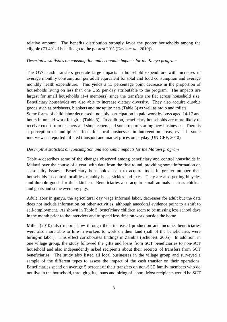
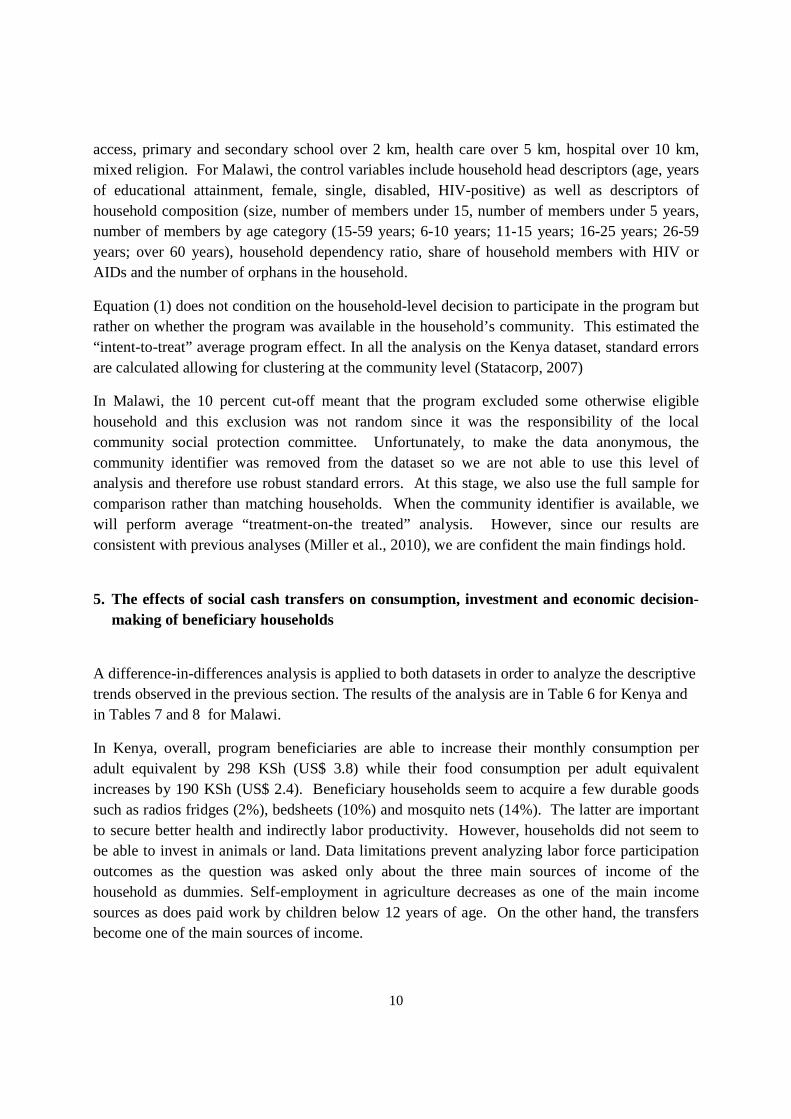
relative amount. The benefits distribution strongly favor the poorer households among the eligible (73.4% of benefits go to the poorest 20% (Davis et al., 2010)). Descriptive statistics on consumption and economic impacts for the Kenya program The OVC cash transfers generate large impacts in household expenditure with increases in average monthly consumption per adult equivalent for total and food consumption and average monthly health expenditure. This yields a 13 percentage point decrease in the proportion of households living on less than one US$ per day attributable to the program. The impacts are largest for small households (1-4 members) since the transfers are flat across household size. Beneficiary households are also able to increase dietary diversity. They also acquire durable goods such as bedsheets, blankets and mosquito nets (Table 3) as well as radio and toilets. Some forms of child labor decreased: notably participation in paid work by boys aged 14-17 and hours in unpaid work for girls (Table 3). In addition, beneficiary households are more likely to receive credit from teachers and shopkeepers and some report starting new businesses. There is a perception of multiplier effects for local businesses in intervention areas, even if some interviewees reported inflated transport and market prices on payday (UNICEF, 2010). Descriptive statistics on consumption and economic impacts for the Malawi program

Table 4 describes some of the changes observed among beneficiary and control households in Malawi over the course of a year, with data from the first round, providing some information on seasonality issues. Beneficiary households seem to acquire tools in greater number than households in control localities, notably hoes, sickles and axes. They are also getting bicycles and durable goods for their kitchen. Beneficiaries also acquire small animals such as chicken and goats and some even buy pigs.

Adult labor in ganyu, the agricultural day wage informal labor, decreases for adult but the data does not include information on other activities, although anecdotal evidence point to a shift to self-employment. As shown in Table 5, beneficiary children seem to be missing less school days in the month prior to the interview and to spend less time on work outside the home.

Miller (2010) also reports how through their increased production and income, beneficiaries were also more able to hire-in workers to work on their land (half of the beneficiaries were hiring-in labor). This effect corroborates findings in Zambia (Schubert, 2005). In addition, in one village group, the study followed the gifts and loans from SCT beneficiaries to non-SCT household and also independently asked recipients about their receipts of transfers from SCT beneficiaries. The study also listed all local businesses in the village group and surveyed a sample of the different types to assess the impact of the cash transfer on their operations. Beneficiaries spend on average 5 percent of their transfers on non-SCT family members who do not live in the household, through gifts, loans and hiring of labor. Most recipients would be SCT

9

eligible if it were not for the 10 percent cut-off point for the program. In addition, beneficiaries seem less likely to resort to begging and theft than control households.

Business reported steadier sales even during the rainy/hungry season and growth in profits. Payment days have become market days and business stock in expectation of heightened sales during those days. Business owners were also more willing to lend to SCT beneficiaries, on the grounds that the transfers provided regular income. However, program implementation issues may jeopardize this strategy (when payments get delayed). Overall, the program therefore seems to generate significant economic impacts on beneficiary households.

4. Empirical strategy

For both impact evaluations, household-level panel data is available in both the treatment and control areas before and after the program was implemented. This enables the use of double difference methods to estimate the average program impact (Duflo et al., 2008 and Ravallion, 2008). The basic estimation equation employing double-difference and incorporating household-level fixed-effects is:

���� � �� ��� ��� �� �� ���� ����,� ��� �����,� ���� ��� ���� (1),

where:

���� is the outcome variable of interest for household i in community c at time t

�� ��� �,��,� � 1 if round=1 (or 2 for Malawi)

��,� ��� � � 1 if the program intervenes in community c at round j

��� all household-level time-invariant factors for household i (fixed effect)

���� the unobserved idiosyncratic household- or community-level, time-varying error

α and δ are unknown coefficients.

δd1 is the double-difference estimator of the average program effect for the first round (relative to the baseline) and δd2 is for the second round relative to the baseline. Given that the control and treatment households differ systematically at baseline, ��,� ��� is correlated with some household- or community-level variables so the analysis will have to correct for these potential biases, using matching techniques, either based on eligibility rules or on propensity scores. For Kenya, the household-level controls at baseline include: household size, number of females, children, adults older than 20 years of age, persons with disability, orphans, ill care providers, whether the head is a female, age of head (linear and square), education dummies, rural, Muslim religion dummy. The community controls include: number of households in the village, car

10

access, primary and secondary school over 2 km, health care over 5 km, hospital over 10 km, mixed religion. For Malawi, the control variables include household head descriptors (age, years of educational attainment, female, single, disabled, HIV-positive) as well as descriptors of household composition (size, number of members under 15, number of members under 5 years, number of members by age category (15-59 years; 6-10 years; 11-15 years; 16-25 years; 26-59 years; over 60 years), household dependency ratio, share of household members with HIV or AIDs and the number of orphans in the household.

Equation (1) does not condition on the household-level decision to participate in the program but rather on whether the program was available in the household’s community. This estimated the “intent-to-treat” average program effect. In all the analysis on the Kenya dataset, standard errors are calculated allowing for clustering at the community level (Statacorp, 2007)

In Malawi, the 10 percent cut-off meant that the program excluded some otherwise eligible household and this exclusion was not random since it was the responsibility of the local community social protection committee. Unfortunately, to make the data anonymous, the community identifier was removed from the dataset so we are not able to use this level of analysis and therefore use robust standard errors. At this stage, we also use the full sample for comparison rather than matching households. When the community identifier is available, we will perform average “treatment-on-the treated” analysis. However, since our results are consistent with previous analyses (Miller et al., 2010), we are confident the main findings hold.

5. The effects of social cash transfers on consumption, investment and economic decision-

making of beneficiary households

A difference-in-differences analysis is applied to both datasets in order to analyze the descriptive trends observed in the previous section. The results of the analysis are in Table 6 for Kenya and in Tables 7 and 8 for Malawi.

In Kenya, overall, program beneficiaries are able to increase their monthly consumption per adult equivalent by 298 KSh (US$ 3.8) while their food consumption per adult equivalent increases by 190 KSh (US$ 2.4). Beneficiary households seem to acquire a few durable goods such as radios fridges (2%), bedsheets (10%) and mosquito nets (14%). The latter are important to secure better health and indirectly labor productivity. However, households did not seem to be able to invest in animals or land. Data limitations prevent analyzing labor force participation outcomes as the question was asked only about the three main sources of income of the household as dummies. Self-employment in agriculture decreases as one of the main income sources as does paid work by children below 12 years of age. On the other hand, the transfers become one of the main sources of income.

11

In Malawi, variables indicative of the economic impacts at the household (Table 7) and child (Table 8) level are explored in regressions with and without control variables. Clustering could not be controlled for at this stage10 so robust standard errors are used.

From the baseline to the second round, a number of economic impacts have taken place. Beneficiary households have increased their per capita monthly food expenditure by MW$ 900 (US$ 6.5) and their non-food expenditure by MW$ 317 (US2.3). As in Kenya, participation in agriculture wage employment and self-employment decrease while transfer income increases, although private transfers (specifically gifts but not remittances) become less frequent. The number of days worked in casual agricultural labor (ganyu) decreased, though the magnitude is smaller than the decrease between baseline and the rainy season. The share of adults working outside the home has also decreased, perhaps conveying a preference for home-based activities, which would be consistent with the minor investments observed in agricultural tools (hoes, axes, sickles) that took place mostly between baseline and the first round and hold up in the second round. In addition, beneficiaries are to buy small animals such as chickens and goats.

Twelve months from the first transfer receipt, the double-difference impact on school attendance is still positive and significant. The effect on number of school days missed by children attending school is also positive and significant, although on a lesser magnitude than between baseline and the first round. There is a slight increase in hours spent on leisure by children in treatment households (half an hour more).

The analysis of double difference results between the baseline and the first round indicators of economic impacts11 point to significant effects for both household and child level variables and shed some light on the timing of investments and the effect of seasonality. March is the end of the rainy season, which is a lean season with little food availability for these households while September is the end of the winter. Days of casual (ganyu) agricultural labor worked are significantly lower among treatment households, the net effect being a drop of approximately one day per month. Food consumption is more important than non-food expenditures in the allocation of the increased liquidity at that moment. A look at asset ownership levels confirms that investments in livestock and in non-agricultural assets are significant but with a net effect of close to zero. Conversely, the double-difference results on agricultural assets reveal positive and significant effects on the number of hoes and sickles owned, indicating that, in the short run, households do make some productive investment, in this case in small tools.

At the child level, positive effects are observed on school enrollment, negative on days of school missed in the previous month and a net negative effect on whether the child worked outside the home when control variables are included in the regression. These outcomes show the net positive effects of the cash transfer on child time use and the household preference for children

10

The data set is missing community identifiers. 11Tables are available upon request.

12

to attend school when liquidity constraints are relaxed. These effects are stronger than on a year-to-year comparison, pointing to the importance of seasonal variations in the liquidity constraints.

In Malawi, the program seems to generate significant economic impacts. Beneficiary households seem to first satisfy their consumption needs and invest in small agricultural tools and animals. This enables them to move out of ganyu labor and to work/hire-in more on their own plot of land. Children in beneficiary households are more able to attend school but their participation in the labor market may still be required in times of severe liquidity constraints. On the other hand, in Kenya, we observe no impacts on investments (although we are missing information on purchases of tools) but we do observe that participation of children in paid work decreases.

To understand whether the results are homogenous among different types of household, we run separate regressions for female and male-headed households; households with one, two, three or more children (since the transfer is flat per household in Kenya); and households with heads younger or older than 60 years of age (because of the demographic differences between households in Kenya and Malawi). Results are summarized in Table 9 for gender of head, Table 10 for household size, and Table 11 for age of head12.

In Kenya, male-headed households are able to acquire farming land but are less likely to acquire radio or mosquito nets. They also spend less on health than female-headed households. On the other hand, teenagers paid work increases among female-headed households even if those children are also more likely to go to school. In Malawi, female-headed households seem more vulnerable as they depend more on casual agricultural labor and include more ill or disabled members. Male-headed households seem to acquire more tools, bicycles and chickens than female-headed ones while female-headed household acquire more goats and spend more on consumption. However, the differences are not significant. In both cases, asset preferences seem to differ according to the gender of the head. It would be interesting to understand why women are less likely to buy tools in Malawi since they seem more involved in agricultural activities overall.

In Kenya, policy-makers and donors are concerned about the heterogeneity of impacts between small and large households given that the transfer is flat, regardless of household size. As described by Azzarri and de la O Campos (2010), impacts on expenditures decrease with household size, including for purchases of household durables such as bed sheets and mosquito nets. Young children (under 12) participation in paid work decreases significantly in households with three or more children as a result of the program (Table 10), maybe because the program covers their opportunity cost.

In Malawi, the transfer follows more closely the number of children with a cap at three. Impacts on expenditures also decrease but less so than in Kenya. However, purchases of small agricultural tools and chicken and goats hold for larger households. Larger households are also 12

Only interactions that are significant for one category are reported.

13

lees likely to participate in casual daily agricultural labor (ganyu) and work less days in this activity than smaller households. One-child households are less likely to keep receiving private gifts.

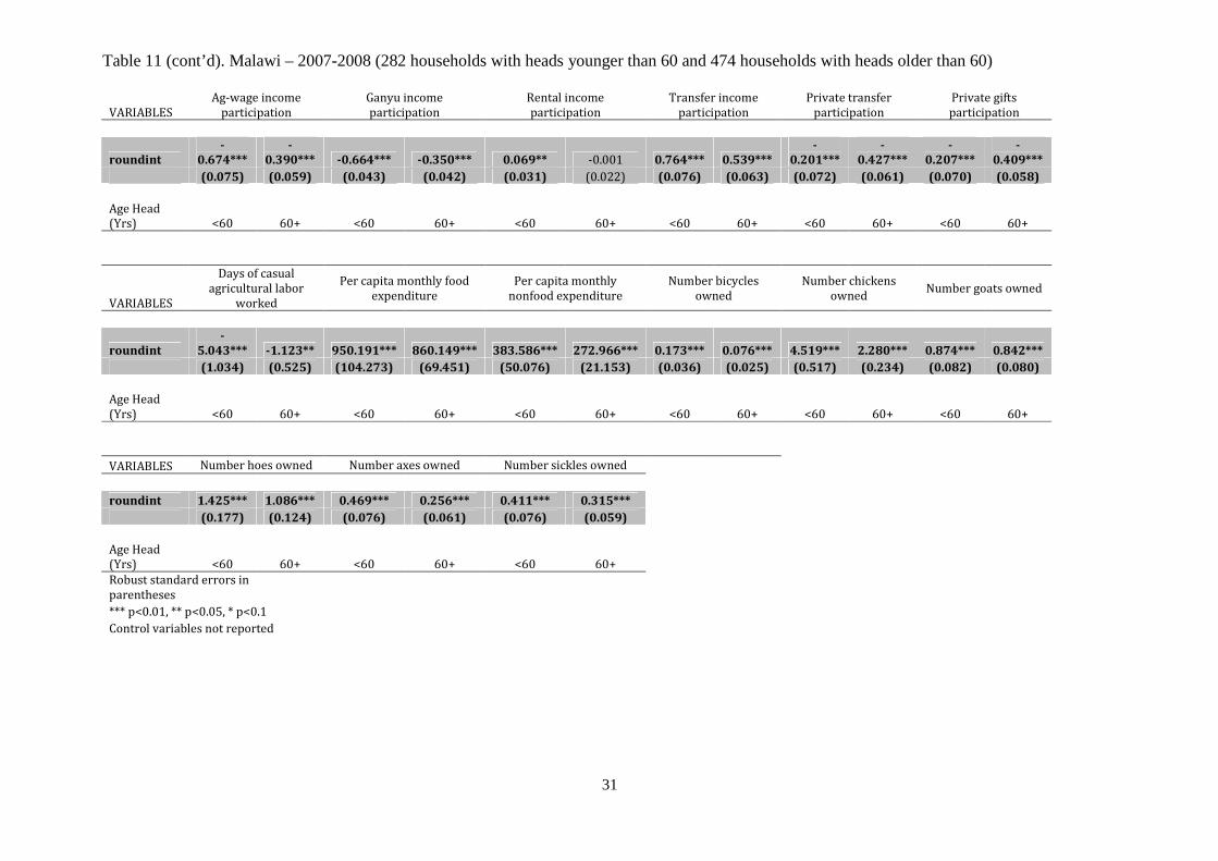
Given the different age profile of beneficiaries in Malawi and Kenya and the concern about differential responses in households where grandparents are taking care of orphan grandchildren (the missing generation households), we also run regressions separately for household heads younger and older than 60 years of age (Table 11). In Kenya, households with elderly heads allocate transfers more towards expenditures (including in health and children’s education) than durable goods. However, the descriptive statistics show that they had higher level of durable goods than younger households, probably reflecting more years of potential accumulation. Children are also healthier and participate less in work than in other types of household, however they spend the same number of hours in unpaid work.

In Malawi, households with older heads are smaller (3.70 members vs. 5.45 for younger households) but disability is more frequent among older households and aged-dependency is higher. As a result, at baseline, their consumption per capita was similar to those of younger households. Households with older heads are less likely to work less in ganyu labor and they also do not decrease their number of days as much as younger households. On the other hand, they are less likely to keep receiving private gifts than younger households as a result of the SCT. Contrary to Kenya their per capita monthly expenditure is less affected by the SCT than younger households. Households with older heads also invest less in durable goods and small animals, even though they did not start with higher levels at baseline.

6. Conclusions

Even among very poor communities, social cash transfers may generate significant economic changes, especially if their amount is large enough to relieve some of the strong liquidity constraints facing poor rural households. We study the impacts of the Kenya OVC Cash Transfer between 2007 and 2009 and the Malawi M’chinji Social Cash Transfer between 2007 and 2008. Both programs target the poor, using community-based targeting complemented with a proxy-means test in the case of Kenya. They successfully reach the poor, with the Malawi program reaching among the most destitute. Beneficiary households in Malawi are older, smaller but with higher dependency ratio than their Kenyan counterparts. They are also much poorer and orphans and vulnerable children are more frequent.

While both programs randomized the intervention at the community-level, households in control and intervention communities, while similar in terms of poverty as measured by household expenditures, differ systematically on other outcomes of interests in Malawi, probably due to the non-uniform application of the targeting criteria at the community level. This illustrates the

14

difficulty of targeting when poverty levels are high and the multi-dimensional aspects of poverty beyond monetary expenditures.

In Kenya, after two years in the program, in addition to positive consumption impacts and increased access to health and education services, beneficiary households seem able to buy some durable goods. However, they do not seem to have been able to acquire animals or land. One potential explanation would the onset of the food price crisis in 2008: households would have been able to maintain consumption but not to invest. The available information does not allow for a detailed analysis of investment in tools, household enterprises or agricultural activities.

As a contrast, in Malawi, after a year in the program, in addition to positive consumption impacts and increased access to health, beneficiary households seem able to buy durable goods such as bicycles, but also small agricultural tools such as hoes, sickles and axes. In addition, they invest in poultry and goats. As a result of the program, adults are also able to get out of agricultural daily labor (ganyu) and additional information from program managers confirms that they work more or hire-in more labor to work on their own plots. Children are less likely to miss school and while they may still engage in the labor market outside the home, they enjoy more leisure. These effects are particularly strong during the winter, when liquidity constraints are further relaxed. Complementary information also describes more community-level multiplier impacts as additional money circulates in these small communities.

These preliminary results are all the more promising given that these programs were operating as the food price crisis hit those countries and the real value of the transfers eroded between baseline and subsequent data collection (20 percent loss in Kenya between 2007 and 2009 and nearly 10 percent in Malawi between 2007 and 2008). While the data at hand do not allow us to qualify whether these impacts will be sustained, one can hope that the increase in landholdings, animals and own production will enable households to maintain higher income streams. However, sustainability remains an issue and some of the impacts may be vulnerable to the program’s operational problems, such as delayed payments in Malawi. The issue of the size of transfer also needs further consideration as it may explain some of the differences in impacts between Kenya and Malawi.

We start exploring possible heterogeneity in impacts according to the gender and age of household heads and the number of children in the household. Households with male heads seem more likely to invest in productive assets in both countries while households with female heads invest more in children’s education (Kenya), spend more on food and health (Kenya and Malawi), seem to depend more on teenager children paid work and participate more in non-agricultural self-employment (Malawi). Further research is needed to understand the barrier that female-headed households face to invest in agricultural activities and other economic activities. type of investments in agriculture that these poor households would favor, especially the ones that are labor-constrained.

15

Older households seem to have accumulated slightly more durables and land than younger households in Kenya and the transfer allows them to increase consumption and expenses related to children. However in Malawi, older households seem more vulnerable overall despite their smaller size. Their income generation strategy is less affected by the program than younger households. The fact that the SCT seems to have displaced private gifts raises questions about the way social networks would work for these households. Overall, older households are not as likely to invest either because of a life-cycle effect or because they are more vulnerable.

Consumption impacts of the transfer decrease with household size, especially when the transfer is flat (Kenya). Children are more likely to be stunted (Kenya) and teenage girls work more hours in unpaid work. However, while in Kenya, they are also less likely to acquire durable goods, in Malawi they do purchase agricultural tools and small animals, consistent with a strategy of increasing work on own plot. This difference is probably explained by the relative size of the transfers in both countries.

Overall, impacts do vary along household demographics characteristics and policy-makers need to be aware of the different income-generation options available to and chosen by different households as the social cash transfers will interact differently with them. Most of data collection so far has focused on human capital and consumption indicators and the information on labor allocation, income, agricultural activities and assets is limited. While our analysis complements other findings, evidence about labor allocation and a wider range of assets would provide a more complete understanding of household behavior. In addition, additional evaluation data from other neighboring countries may shed some light on the dynamics at play.

16

Table 1: Basic Information about Country Case Programs

Country Kenya Malawi Name of program

OVC Cash Transfer Social Cash Transfer

Institutional setting

OVC Transfer Secretariat in the Ministry of Gender, Children and Social Development

Department of Poverty Reduction and Social Protection in the Ministry of Economic Planning and Development

Start date 2004-2005 (pre-pilot); 2006-2009 (pilot)

2006 (expanded in 2008)

End date None None, pending funding Expansion plans

Yes. 139,000 hhs (458,000 OVCs) in 47 districts by 2012

Yes, pending approval by government. 300,000 hh w/ 910,000 children by 2015

Target Orphans living in extreme poverty Ultra-poor and labor constrained HHs (bottom 10%)

Targeting mechanism

Three Step Process: 1) Community Targeting 2) Means Testing 3) Community Consultation and Grievance Procedure

Community-Based (community social protection committees as village level) w/ checks from village development committee

Urban/rural Urban and Rural Rural Conditionali-ty

Yes in random districts. Testing both health and schooling conditions and non-conditions.

No, but bonus for school attendance. Bonus is US$1.4 (MK 200) for primary and US$2.8 (MK 400) for secondary

Amount 1500 Ksh (US$19.50) per hh per month, irrespective of size

Based on hh size per month: 1= US$4.3 (MK 600) 2 = US$7.1 3 = US$10 4+ = US$12.9 Average transfer including schooling bonuses is US$ 14.

Delivery mechanism

Postal Office in 7 districts. District Children's Offices in 30 districts. Both bi-monthly

Monthly through government.

# of hh 82,000 24,300 # participants

270,000 OVCs 51,410 people (33,700 children, of which 25,780 are orphans)

# districts 37 7 # districts in country

115 28

Table 2: Evaluation design for the country case programs Kenya OVC CCT Malawi SCT Timing Baseline data in 8 districts in March-

Aug 2007. Follow-up in March-July 2009. 2nd follow-up planned in 2011

Baseline data in Mchinji district in March 2007. Follow-up in September 2007 and March 2008.

Number of hh

2,255 hh (1,513 in treatment communities)

758 hh (372 in intervention communities)

Randomization

Community-level. Eligible households by community and PMT.

Community-level. Eligible households by committee.

Methods PSM and DiD PSM and DiD Partner First stage Oxford Policy Management ,

currently University of North Carolina (UNC)

First stage Boston University, currently UNC

17

Table 3: Descriptive statistics on income sources, durable and asset holdings among eligible households in treatment and control areas in Kenya

Baseline Round 1

HOUSEHOLD LEVEL STATISTICS

Control

(n=747)

Treated

(n= 1,494)

Control

(n=572)

Treated

(n=1,282)

Income: Participation in three main activities

Household has no work 0.03 0.04 0.05** 0.08**

Main HH income source is wage employment 0.06** 0.03** 0.09** 0.05**

Main HH income source is ag self-employment 0.6 0.62 0.45* 0.39*

Main HH income source is non-ag self-employment 0.21 0.2 0.31 0.27

Main HH income source is own business / employer 0.06 0.08 0.09 0.08

Main HH income source is gifts or transfers (incl OVC cash) 0.05 0.06 0.05*** 0.21***

(OVC transfer not in baseline)

Main HH income source is OVC-CT transfers 0.00*** 0.19***

(OVC transfer not in baseline)

Child Employment

Children (aged 12 to 18) work for money 0.69 0.67 0.55** 0.62**

Young children (aged under 12) work for money 0.25 0.3 0.20*** 0.12***

Expenditures

Mean monthly real HH consumptionper adult equivalent 1513.87 1574.81 1542.36*** 1865.00***

Mean monthly real HH food consumptionper adult equivalent 979.05 1012.97 1110.22*** 1337.23***

Mean monthly health expenditure pc (excluding AIDS) 39.80 35.54 31.66* 38.73*

Mean monthly education expenditure per child 115.16 112.77 124.37 150.76

Assets and durables

HH owns real estate property (e.g. household dwelling) 0.88 0.86 0.91 0.93

Acres of farming land owned by household 1.99 1.78 2.90** 1.77**

Household owns radio 0.4 0.43 0.47*** 0.56***

Household owns telephone 0.1 0.13 0.32 0.31

Household owns bucket 0.89 0.9 0.93 0.94

Household owns table 0.85* 0.89* 0.87 0.9

Household owns chairstool 0.93 0.94 0.94 0.95

Household owns bedsheets 0.82 0.81 0.82*** 0.92***

Household owns blankets 0.87 0.9 0.89** 0.93**

Household owns mosquitonet 0.64 0.65 0.73*** 0.85***

Household owns livestock 0.84 0.83 0.8 0.82

Number of cattle owned 1.34 1.21 1.58 1.44

Number of donkeys owned 0.04 0.04 0.08 0.07

Number of camels owned 0.05 0.07 0.09 0.05

Number of goats owned 2.33 2.01 0 0

Number of sheep owned 1.18** 0.53** 1.19 0.75

Number of pigs owned 0.03 0.02 0.03 0.07

Number of poultry owned 4.65* 3.89* 3.42 3.32

Number of small animals owned 3.54 2.56 1.23 0.83

18

HOUSEHOLD LEVEL STATISTICS

Control

(n=747)

Treated

(n=

1,494)

Control

(n=572)

Treated

(n=1,282)

Child Labour

Participates in paid work (ages 6-13) 0.03 0.04 0.01 0.01

Participates in paid work (ages 14-17) 0.14 0.12 0.07** 0.04**

Boys participate in paid work (ages 14-17) 0.19 0.13 0.09* 0.05*

Girls participate in paid work (ages 14-17) 0.09 0.11 0.04 0.02

Participates in unpaid work (ages 6-13) 0.77 0.78 0.85** 0.79**

Participates in unpaid work (ages 14-17) 0.84* 0.89* 0.88* 0.83*

Hours in unpaid work (ages 6-13) 13.98** 15.39** 9.96** 9.00**

Hours in unpaid work (ages 14-17) 17.56** 20.48** 12.78 12.02

Boys: hours in unpaid work (ages 6-13) 13.83 14.78 9.84 9.14

Girls: hours in unpaid work (ages 6-13) 14.19* 16.07* 10.10* 8.86*

Boys: hours in unpaid work (ages 14-17) 17.21* 20.35* 11.56 11.17

Girls: hours in unpaid work (ages 14-17) 18.00 20.68 14.62 13.13

Notes: asterisk denotes statistically different means based on t-test using robust standard errors. * significant at 10%, ** significant at 5% and *** significant at 1%.

19

Table 4: Descriptive statistics on durable and animal holdings, and adult labor in treatment and control areas in Malawi Baseline Mar-07 Round 1 Sep-07 Round 2 Mar-08

HOUSEHOLD LEVEL STATISTICS

Control

(n=386)

Treated

(n=372)

Control

(n=386)

Treated

(n=372)

Control

(n=387)

Treated

(n=371)

Income: Participation

Salaried employment 0.02** 0.05** 0 0.01 0.02 0.03

Agricultural wage labour 0.29 0.33 0.66*** 0.29*** 0.69*** 0.26***

Ganyu labour (not reported at baseline) 0 0 0.65*** 0.29*** 0.68*** 0.25***

On-farm self employment 0.31 0.33 0.38 0.34 0.33** 0.41**

Rental income 0.03 0.03 0.03 0.03 0.01** 0.04**

Transfer income 0.38* 0.44* 0.35*** 1.09*** 0.41*** 1.09***

Public transfer income 0.03 0.03 0.03*** 0.99*** 0.02*** 0.99***

Public transfers: government grants 0.02 0.01 0.01*** 0.98*** 0.01*** 0.96***

Private transfers: gifts from family/friends 0.31** 0.39** 0.27*** 0.06*** 0.35*** 0.09***

Other income sources 0.07 0.07 0.05 0.03 0.04 0.04

Employment

share of adults in household that worked outside the home 0.5 0.52 0.04 0.03 0.10* 0.07*

number of ganyu days worked per adult in household 3.83 3.93 2.91*** 0.81*** 3.00*** 0.54***

working age adults(19-64)not ill/disable 0.49*** 0.64*** 0.57*** 0.77*** 0.57*** 0.88***

Expenditures

No health expenditure 0.69*** 0.59*** 0.70*** 0.35*** 0.63*** 0.24***

Monthly school expenditure per child 190.33** 288.96** 88.41 158.54 . 142.3

Per capita monthly food expenditure 125.32 134.19 85.59*** 858.31*** 141.42*** 1055.53***

Per capita monthly non-food expenditure 45.86 51.4 73.46*** 305.89*** 90.78*** 422.15***

Assets

number of hoes 0.88 0.88 1.53*** 2.22*** 1.49*** 2.80***

number of axes 0.28 0.33 0.18*** 0.54*** 0.20*** 0.60***

number of sickles 0.17*** 0.27*** 0.13*** 0.59*** 0.18*** 0.63***

number of beer drums (used of iga) 0 0.01 0.01* 0.03* 0.03 0.03

number of bicycles 0.01 0.01 0.01*** 0.13*** 0.02*** 0.13***

number of chickens 0.1 0.13 0.18*** 2.08*** 0.21*** 3.43***

number of goats 0.02 0.01 0.03*** 0.52*** 0.02*** 0.87***

number of cattle 0 0 0.01 0.01 0 0.02

number of pigs 0 0 0.00*** 0.25*** 0.00*** 0.23***

changes of clothing 2.08 2.07 2.17*** 4.07*** 1.81*** 3.87***

number of metallic plates N/A N/A 1.76*** 5.33*** 2.13*** 7.31***

number of metal pots N/A N/A 0.98*** 1.99*** 1.34*** 2.61***

number of pounding mortars N/A N/A 0.45*** 0.70*** 0.59*** 1.13***

number of panga knives N/A N/A 0.09*** 0.40*** 0.12*** 0.52***

number of mats N/A N/A 0.97*** 1.80*** 1.21*** 2.60***

number of pails/buckets 0 N/A 0.71*** 1.66*** 0.85*** 2.11***

20

Table 5: Descriptive statistics on children activities in treatment and control areas in Malawi

Baseline (March 07) Round 1 (Sep 07) Round 2 (March 08)

BY TREATMENT/CONTROL HOUSEHOLDControl Treated Control Treated Control Treated

Number of children 673 909 673 909 673 909

child currently attending school 0.85** 0.89** 0.82*** 0.92*** 0.84*** 0.93***

[0.36] [0.31] [0.38] [0.27] [0.37] [0.25]

child worked outside home 0.3 0.28 0.37*** 0.44*** 0.34 0.36

[0.46] [0.45] [0.48] [0.50] [0.47] [0.48]

number of hours worked outside home 3.01 2.75 1.30*** 1.05*** 2.76** 2.28**

[3.30] [2.69] [1.70] [0.61] [1.84] [2.38]

child did any leisure activities 0.71 0.74 0.76 0.76 0.77 0.78

[0.45] [0.44] [0.43] [0.43] [0.42] [0.41]

hours spent on leisure activities 3.27 2.98 2.42** 2.21** 2.69** 2.96**

[4.03] [2.58] [1.42] [1.43] [1.84] [2.45]

number of days missed school past month 3.12 2.81 2.67*** 1.62*** 2.28*** 1.15***

[4.76] [3.67] [3.69] [3.35] [3.68] [2.33]

household is headed by child 0 0.01 0 0.01 0.01 0.01

[0.04] [0.07] [0.04] [0.07] [0.10] [0.08]

Notes: asterisk denotes statistically different means based on t-test using robust standard errors. Standard deviations in square brackets. * significant at 10%, ** significant at 5% and *** significant at 1%

21

Table 6: Double-difference estimates of the Kenya CT-OVC household-level effects between 2007 and 2009

VARIABLES

round 0.03 0.03 -0.12** -0.12*** 0.09** 0.09** 0.02 0.02 -0.02 -0.02 -0.13*** -0.13*** 0.01 0.01

(0.04) (0.03) (0.05) (0.04) (0.04) (0.04) (0.02) (0.02) (0.03) (0.02) (0.04) (0.03) (0.04) (0.04)

intervention -0.06** -0.05** 0.06 0.05 -0.01 0.01 0.03* 0.03* -0.02 -0.02 -0.06 -0.05* 0.06* 0.07**

(0.03) (0.02) (0.04) (0.03) (0.03) (0.03) (0.02) (0.02) (0.02) (0.02) (0.03) (0.03) (0.03) (0.03)

round*int -0.01 -0.01 -0.09* -0.09** -0.02 -0.02 -0.02 -0.02 0.15*** 0.15*** 0.08 0.08* -0.19*** -0.19***

(0.04) (0.03) (0.06) (0.04) (0.05) (0.05) (0.03) (0.02) (0.04) (0.03) (0.05) (0.04) (0.05) (0.05)

Constant 0.10*** -0.02 0.54*** 0.35 0.23*** 0.59** 0.05*** 0.22 0.07*** -0.05 0.73*** 0.62** 0.24*** -0.33

(0.03) (0.16) (0.04) (0.27) (0.03) (0.27) (0.01) (0.14) (0.02) (0.18) (0.03) (0.26) (0.03) (0.23)

Control variables? NO YES NO YES NO YES NO YES NO YES NO YES NO YES

Observations 1,924 1,924 1,924 1,924 1,924 1,924 1,924 1,924 1,924 1,924 1,924 1,924 1,924 1,924

R-squared 0.02 0.23 0.03 0.32 0.01 0.15 0.00 0.16 0.03 0.18 0.01 0.17 0.02 0.12

VARIABLES

round -37.18 -37.18 110.25* 110.29** -14.97* -14.97* 3.42 4.65 0.76 0.76 0.03 0.03 0.02 0.02

(94.02) (80.95) (57.26) (51.06) (8.80) (7.75) (33.25) (28.50) (0.58) (0.57) (0.05) (0.04) (0.04) (0.03)

intervention -1.89 -25.48 30.68 10.81 -13.08* -14.63** -24.58 -24.33 -0.24 -0.22 -0.01 -0.00 -0.01 -0.02

(85.68) (72.93) (47.54) (43.21) (7.88) (6.75) (27.05) (24.02) (0.21) (0.20) (0.04) (0.03) (0.03) (0.03)

round*int 298.64*** 298.64*** 190.98*** 191.13*** 16.91* 16.91** 33.67 31.94 -0.65 -0.65 0.08 0.08 0.10** 0.10***

(106.52) (94.01) (68.42) (62.41) (9.36) (8.41) (36.08) (31.51) (0.64) (0.63) (0.06) (0.05) (0.04) (0.04)

Constant 1,581.92*** 2,366.26*** 983.18*** 1,540.45*** 47.97*** -24.59 138.68*** -84.85 2.10*** 0.83 0.44*** 0.39 0.80*** 0.88***

(77.00) (452.24) (39.78) (310.55) (7.52) (31.43) (24.96) (146.26) (0.18) (1.98) (0.04) (0.28) (0.03) (0.21)

Control variables? NO YES NO YES NO YES NO YES NO YES NO YES NO YES

Observations 1,924 1,924 1,920 1,920 1,924 1,924 1,907 1,907 1,924 1,924 1,924 1,924 1,924 1,924

R-squared 0.02 0.19 0.04 0.17 0.01 0.11 0.00 0.20 0.00 0.05 0.01 0.21 0.01 0.20

Robust standard errors in parentheses

*** p<0.01, ** p<0.05, * p<0.1

Main Income is Own-

Business Main Income is Transfers

Monthly Education Exp.

per Child

Child Paid Work

12-18 years

Owned

Farming land

Household Owns

Radio

Household Owns

Bedsheet

Child Paid Work

below 12

Main Income is Wage

Employment

Monthly Exp. per

Adult Equivalent

Monthly Food Exp. per

Adult Equivalent

Monthly Health Exp. per

Capita

Main Income is Self

Employment Agr

Main Income is Self

Employment Non-Agr

Table 6 (cont’d): Double-difference estimates of the Kenya CT-OVC household-level effects between 2007 and 2009

22

VARIABLES

Number of Cattle

Owned

Number of Donkeys

Owned

Number of Camels

Owned

Number of Poultry

Owned

round 0.25 0.25 0.04 0.04 0.05 0.05 -0.94* -0.94**

(0.21) (0.19) (0.04) (0.03) (0.05) (0.05) (0.51) (0.45)

intervention 0.05 -0.02 0.01 0.01 0.02 0.01 -0.15 -0.07

(0.17) (0.16) (0.02) (0.02) (0.03) (0.03) (0.48) (0.47)

round*int -0.05 -0.05 -0.02 -0.02 -0.07 -0.07 0.08 0.08

(0.25) (0.23) (0.04) (0.04) (0.06) (0.05) (0.61) (0.56)

Constant 1.18*** -0.18 0.03*** -0.27* 0.03 -0.98*** 4.33*** 4.90*

(0.15) (2.06) (0.01) (0.16) (0.02) (0.38) (0.37) (2.65)

Control

variables? NO YES NO YES NO YES NO YES

Observations 1,924 1,924 1,924 1,924 1,924 1,924 1,924 1,924

R-squared 0.00 0.14 0.00 0.19 0.00 0.19 0.01 0.13

23

Table 7: Double-difference estimates of the Malawi M’chinji SCT household-level effects between 2007 and 2008

VARIABLES

round -0.001 -0.005 0.201*** 0.398*** 0.342*** 0.685*** 0.007 0.014 -0.006 -0.015 -0.148*** -0.301*** 0.018 0.030

(0.005) (0.010) (0.017) (0.032) (0.012) (0.022) (0.017) (0.034) (0.005) (0.010) (0.015) (0.031) (0.018) (0.037)

intervention 0.041** 0.022* 0.274*** 0.011 0.218*** -0.022*** -0.011 0.013 -0.002 0.009 0.141** 0.064* -0.245*** 0.084**

(0.021) (0.013) (0.053) (0.035) (0.016) (0.007) (0.054) (0.035) (0.020) (0.013) (0.056) (0.036) (0.056) (0.036)

roundint -0.008 -0.015 -0.236*** -0.484*** -0.218*** -0.443*** 0.031 0.054 0.011 0.025 -0.044** -0.088** 0.308*** 0.617***

(0.009) (0.018) (0.024) (0.047) (0.016) (0.032) (0.024) (0.049) (0.009) (0.018) (0.022) (0.044) (0.024) (0.049)

Constant 0.019* -0.003 0.089** 0.431*** -0.342*** 0.034 0.306*** 0.316*** 0.032*** 0.078** 0.573*** 0.536*** 0.361*** 0.378***

(0.011) (0.034) (0.037) (0.098) (0.012) (0.068) (0.037) (0.096) (0.012) (0.034) (0.039) (0.090) (0.040) (0.106)

Control variables? NO YES NO YES NO YES NO YES NO YES NO YES NO YES

Observations 1,516 1,497 1,516 1,497 1,516 1,497 1,516 1,497 1,516 1,497 1,516 1,497 1,516 1,497

R-squared 0.007 0.039 0.128 0.172 0.440 0.473 0.006 0.027 0.004 0.015 0.139 0.174 0.276 0.294

VARIABLES

round -0.008 -0.015 -0.005 -0.013 0.016 0.028 -0.017* -0.033* 0.019 0.034 -0.014* -0.027*

(0.006) (0.012) (0.004) (0.009) (0.018) (0.036) (0.009) (0.017) (0.017) (0.034) (0.008) (0.017)

intervention -0.484*** 0.002 -0.490*** -0.009 0.227*** 0.078** 0.001 0.003 0.252*** 0.096*** 0.007 -0.003

(0.021) (0.013) (0.014) (0.008) (0.055) (0.036) (0.029) (0.020) (0.054) (0.035) (0.029) (0.019)

roundint 0.485*** 0.969*** 0.482*** 0.965*** -0.173*** -0.347*** -0.011 -0.024 -0.171*** -0.339*** -0.004 -0.009

(0.009) (0.019) (0.007) (0.014) (0.024) (0.047) (0.011) (0.023) (0.022) (0.045) (0.012) (0.024)

Constant 0.041*** -0.049 0.023** -0.016 0.346*** 0.403*** 0.097*** 0.073 0.292*** 0.334*** 0.084*** 0.185***

(0.014) (0.039) (0.010) (0.035) (0.039) (0.102) (0.021) (0.048) (0.037) (0.090) (0.020) (0.053)

Control variables? NO YES NO YES NO YES NO YES NO YES NO YES

Observations 1,516 1,497 1,516 1,497 1,516 1,497 1,516 1,497 1,516 1,497 1,516 1,497

R-squared 0.844 0.847 0.906 0.909 0.070 0.103 0.013 0.030 0.066 0.095 0.005 0.031

Robust standard errors in parentheses

*** p<0.01, ** p<0.05, * p<0.1

Ag-wage income

participation

Ganyu income

participation

On-farm income

participation

Rental income

participation

Self employment

participation

Transfer income

participation

Public transfer income

participation

Public cash transfer

participation

Private transfer

participation

Private remittances

participation

Private gifts

participation

Wage income

participation

Other income

participation

24

Table 7 (cont’d): Double-difference estimates of the Malawi M’chinji SCT household-level effects between 2007 and 2008

VARIABLES

round -0.415** -0.778** -0.200*** -0.403*** 8.048 15.839 22.461*** 45.320*** 0.057** 0.073 0.001 -0.013 -0.001 -0.004

(0.203) (0.381) (0.012) (0.023) (10.027) (21.637) (3.439) (6.759) (0.023) (0.053) (0.006) (0.015) (0.001) (0.003)

intervention 1.331* -0.379 0.053 0.002 -443.748*** 49.038** -157.373*** 23.418*** -1.564*** -0.067 -0.432*** -0.040*** -0.013* -0.004

(0.684) (0.426) (0.045) (0.027) (41.738) (21.677) (14.586) (7.605) (0.134) (0.050) (0.032) (0.015) (0.007) (0.003)

roundint -1.261*** -2.686*** -0.028* -0.065** 452.622*** 898.031*** 162.912*** 316.609*** 1.594*** 3.229*** 0.427*** 0.852*** 0.011* 0.020*

(0.261) (0.500) (0.017) (0.032) (31.607) (58.991) (12.136) (23.541) (0.130) (0.259) (0.029) (0.059) (0.006) (0.012)

Constant 4.236*** 5.733*** 0.698*** 0.728*** 117.273*** 590.249*** 23.399*** 242.115*** 0.044 0.496 0.017 -0.246** 0.004 0.001

(0.493) (0.942) (0.032) (0.063) (20.856) (114.248) (6.178) (62.119) (0.032) (0.426) (0.011) (0.106) (0.004) (0.011)

Control variables? NO YES NO YES NO YES NO YES NO YES NO YES NO YES

Observations 1,516 1,497 1,506 1,497 1,516 1,497 1,516 1,497 1,516 1,497 1,516 1,497 1,516 1,497

R-squared 0.065 0.187 0.299 0.392 0.301 0.362 0.310 0.345 0.246 0.273 0.299 0.333 0.004 0.016

VARIABLES

round 0.301*** 0.551*** -0.042*** -0.082*** 0.002 -0.004 0.012* 0.022 0.005 0.007

(0.030) (0.057) (0.016) (0.029) (0.014) (0.027) (0.007) (0.014) (0.005) (0.010)

intervention -0.659*** -0.137*** -0.131** 0.038 -0.087* 0.075** 0.012 0.008 -0.063*** -0.012

(0.065) (0.040) (0.054) (0.031) (0.049) (0.029) (0.012) (0.006) (0.015) (0.008)

roundint 0.657*** 1.281*** 0.177*** 0.340*** 0.180*** 0.354*** -0.004 -0.006 0.058*** 0.117***

(0.056) (0.102) (0.026) (0.048) (0.024) (0.047) (0.009) (0.018) (0.011) (0.021)

Constant 0.582*** 1.012*** 0.324*** 0.297*** 0.171*** 0.191* -0.009 -0.039 0.008 0.081*

(0.038) (0.229) (0.036) (0.095) (0.031) (0.104) (0.008) (0.029) (0.009) (0.043)

Control variables? NO YES NO YES NO YES NO YES NO YES

Observations 1,516 1,497 1,516 1,497 1,516 1,497 1,516 1,497 1,516 1,497

R-squared 0.342 0.468 0.080 0.251 0.137 0.220 0.004 0.015 0.062 0.102

Robust standard errors in parentheses

*** p<0.01, ** p<0.05, * p<0.1

Number chickens owned Number goats owned Number cattle owned

Number hoes owned Number axes owned Number sickles owned Number beerdrum

Days of casual

agricultural labor

worked

Share of adults in

household worked

outside home

Per capita monthly food

expenditure

Per capita monthly

nonfood expenditure

Number bicycles owned

25

Table 8: Double-difference estimates of the Malawi M’chinji SCT child-level effects between 2007 and 2008

Child currently

attending school

Child worked outside

home

Hours child worked

outside home Any leisure activities

Hours child spent on

leisure

School days missed in

last month

(1) (2) (1) (2) (1) (2) (1) (2) (1) (2) (1) (2)

round -0.010 0.002 0.039 0.002 -0.250 -0.252 0.058** 0.017 -0.574*** -0.392**

-

0.837*** -0.761***

(0.022) (0.021) (0.025) (0.023) (0.261) (0.244) (0.024) (0.019) (0.200) (0.182) (0.280) (0.281)

intervention 0.043** 0.034* -0.023 -0.019 -0.265 -0.101 0.025 0.008 -0.288 -0.249 -0.310 -0.261

(0.019) (0.019) (0.023) (0.022) (0.287) (0.262) (0.023) (0.020) (0.209) (0.180) (0.266) (0.268)

roundint 0.051* 0.043* 0.043 0.043 -0.217 -0.321 -0.016 -0.009 0.553** 0.494** -0.815**

-

0.912***

(0.026) (0.025) (0.033) (0.031) (0.338) (0.312) (0.031) (0.025) (0.242) (0.224) (0.325) (0.325)

Constant 0.849*** -0.127 0.300*** -0.004 3.010*** 3.748** 0.715*** -0.358*** 3.267*** 3.227*** 3.116*** 3.668***

(0.016) (0.095) (0.018) (0.068) (0.231) (1.661) (0.017) (0.061) (0.183) (0.764) (0.224) (0.925)

Control variables? NO YES NO YES NO YES NO YES NO YES YES NO

Observations 2,667 2,617 3,164 3,109 1,011 987 3,164 3,109 2,380 2,337 2,342 2,299

R-squared 0.014 0.103 0.005 0.188 0.011 0.119 0.004 0.347 0.005 0.061 0.046 0.062

Robust standard errors in parentheses

*** p<0.01, ** p<0.05, * p<0.1

26

Table 9: Double-difference estimates by gender of household head Note: only significant interactions for at least one category reported. Kenya – 2007-2009 (632 male-headed households and 1,292 female-headed households)

VARIABLES

round*int -0.16** -0.06 0.13*** 0.16*** 0.00 0.13** -0.17* -0.19*** -0.91* -0.65

(0.07) (0.05) (0.04) (0.04) (0.07) (0.06) (0.08) (0.06) (0.53) (0.93)

Head gender MALE FEMALE MALE FEMALE MALE FEMALE MALE FEMALE MALE FEMALE

VARIABLES

round*int 205.87 349.15*** 159.39* 217.45*** 2.83 23.39** 0.04 0.10* 0.16*** 0.07 0.03 0.19***

(154.27) (112.66) (88.79) (76.93) (9.99) (10.66) (0.08) (0.06) (0.06) (0.05) (0.08) (0.06)

Head gender MALE FEMALE MALE FEMALE MALE FEMALE MALE FEMALE MALE FEMALE MALE FEMALE

Robust standard errors in parentheses

*** p<0.01, ** p<0.05, * p<0.1

Household Owns

Mosquitonet

Main Income is

Transfers

Child Paid Work

below 12

Child Paid Work

12-18 years

Owned

Farming land

Household Owns

Radio

Household Owns

Bedsheet

Monthly Exp. per

Adult Equivalent

Monthly Food Exp. per

Adult Equivalent

Monthly Health Exp.

per Capita

Main Income is Self

Employment Agr

27

Table 9 (cont’d) Malawi – 2007-2008 (271 male-headed households and 485 female-headed households)

Malawi Control variables not reported

VARIABLES

roundint -0.526*** -0.452*** -0.447*** -0.435*** -0.020 -0.134** 0.625*** 0.611*** 0.973*** 0.967*** 0.942*** 0.977*** -0.335*** -0.355*** -0.335*** -0.344***

(0.079) (0.059) (0.054) (0.040) (0.080) (0.053) (0.081) (0.061) (0.029) (0.024) (0.021) (0.018) (0.079) (0.059) (0.074) (0.056)

Head Gender Male Female Male Female Male Female Male Female Male Female Male Female Male Female Male Female

VARIABLES

roundint -3.118*** -2.358*** 795.277*** 969.672*** 258.887*** 354.882*** 0.200*** 0.070*** 3.809*** 2.874*** 0.718*** 0.921***

(0.761) (0.642) (83.043) (82.206) (24.314) (36.593) (0.046) (0.020) (0.385) (0.341) (0.086) (0.076)

Head Gender Male Female Male Female Male Female Male Female Male Female Male Female

VARIABLES

roundint 1.507*** 1.119*** 0.407*** 0.303*** 0.364*** 0.345***

(0.186) (0.117) (0.096) (0.052) (0.091) (0.052)

Head Gender Male Female Male Female Male Female

Robust standard errors in parentheses

*** p<0.01, ** p<0.05, * p<0.1

Control variables not reported

Private transfer Private gifts

Number chickens

ownedNumber goats owned

Number hoes owned Number axes owned Number sickles owned

Days of casual

agricultural labor

Per capita monthly

food expenditure

Per capita monthly

nonfood expenditure

Number bicycles

owned

Ag-wage income Ganyu income Self employment Transfer income Public transfer income Public cash transfer

28

Table 10: Double-difference estimates by household size (one, two, three or more children) Kenya – 2007-2009 (312 one-child, 457 two-children and 1,138 three or more children households)

VARIABLES

Main Income is

Self Employment Agr

Main Income is

Self Employment Non-Agr

Main Income is

Transfers

Child Paid Work

below 12

round*int -0.19* -0.08 -0.06 0.01 -0.16** 0.00 0.18*** 0.18*** 0.14*** -0.05 -0.04 -0.28***

(0.10) (0.09) (0.06) (0.10) (0.08) (0.06) (0.06) (0.07) (0.04) (0.12) (0.09) (0.06)

No of Children 1 2 3+ 1 2 3+ 1 2 3+ 1 2 3+

VARIABLES

Monthly Exp. per

Adult Equivalent

Monthly Food Exp. per Adult

Equivalent

Monthly Health Exp.

per Capita

Household Owns

Bedsheet

Household Owns

Mosquitonet

round*int 663.46** 249.64 201.13* 415.77** 188.05* 120.86 30.65* 28.12** 9.83 0.33*** 0.14 0.03 0.32** 0.19* 0.09

(263.25) (158.08) (116.91) (187.91) (113.62) (74.94) (16.13) (12.53) (11.54) (0.11) (0.09) (0.04) (0.13) (0.10) (0.06)

No of Children 1 2 3+ 1 2 3+ 1 2 3+ 1 2 3+ 1 2 3+

Robust standard errors in parentheses

*** p<0.01, ** p<0.05, * p<0.1

29

Table 10 (cont’d) Malawi – 2007-2008 (131 one-child, 116 two-children and 264 three or more children households)

Malawi

VARIABLES

roundint -0.560*** -0.479*** -0.693*** -0.481*** -0.596*** -0.715*** -0.185* -0.063 0.005 0.590*** 0.698*** 0.726*** -0.335*** -0.261** -0.244***

(0.116) (0.117) (0.078) (0.077) (0.071) (0.045) (0.111) (0.108) (0.075) (0.120) (0.130) (0.082) (0.118) (0.124) (0.077)

N Children 1 2 3+ 1 2 3+ 1 2 3+ 1 2 3+ 1 2 3+

VARIABLES

roundint -0.337*** -0.172 -0.264*** -3.488*** -3.079** -4.117*** 1,008.505***823.938*** 713.798*** 283.126*** 320.892*** 253.159*** 0.022 0.187*** 0.142***

(0.111) (0.114) (0.075) (0.897) (1.241) (1.108) (197.158) (109.936) (64.143) (31.213) (35.568) (22.220) (0.048) (0.056) (0.034)

N Children 1 2 3+ 1 2 3+ 1 2 3+ 1 2 3+ 1 2 3+

VARIABLES

roundint 2.329*** 3.835*** 3.885*** 0.708*** 1.066*** 1.001*** 1.185*** 1.199*** 1.521*** 0.255** 0.360*** 0.428*** 0.385*** 0.409*** 0.352***

(0.489) (0.664) (0.447) (0.118) (0.151) (0.090) (0.243) (0.255) (0.210) (0.111) (0.109) (0.082) (0.118) (0.114) (0.078)

N Children 1 2 3+ 1 2 3+ 1 2 3+ 1 2 3+ 1 2 3+

Robust standard errors in parentheses

*** p<0.01, ** p<0.05, * p<0.1

Control variables not reported

Ag-wage income participation Ganyu income participation Self employment participation Transfer income participation Private transfer participation

Number axes owned Number sickles owned

Per capita monthly nonfood Number bicycles owned

Number chickens owned Number goats owned Number hoes owned

Private gifts participation Days of casual agricultural labor Per capita monthly food

30

Table 11: Double-difference estimates by age of household head (below or above 60 years) Kenya – 2007-2009 (1,090 households with heads younger than 60 and 834 households with heads older than 60)

VARIABLES

Main Income is Self

Employment Agr

Main Income is

Transfers

Child Paid Work

12-18 years

Child Paid Work

below 12

Monthly Exp. per

Adult Equivalent

Monthly Food Exp.

per Adult Equivalent

round*int -0.09* -0.08 0.14*** 0.14*** 0.02 0.09 -0.34*** 0.06 127.27 551.58*** 69.95 377.89***

(0.05) (0.07) (0.04) (0.04) (0.06) (0.07) (0.06) (0.07) (125.96) (116.16) (80.38) (90.49)

Age Head

(Yrs) <60 60+ <60 60+ <60 60+ <60 60+ <60 60+ <60 60+

VARIABLES

Monthly Health Exp.

per Capita

Monthly Education

Exp. per Child

Owned

Farming land

Household Owns

Radio

Household Owns

Bedsheet

Household Owns

Mosquitonet

round*int 15.21 18.18** 17.05 45.55* -0.55 -0.68* 0.11* 0.04 0.12*** 0.09 0.15** 0.13*

(11.34) (9.11) (44.81) (27.47) (0.99) (0.41) (0.06) (0.07) (0.04) (0.06) (0.06) (0.07)

Age Head

(Yrs) <60 60+ <60 60+ <60 60+ <60 60+ <60 60+ <60 60+

Robust standard errors in

parentheses

*** p<0.01, ** p<0.05, * p<0.1

31

Table 11 (cont’d). Malawi – 2007-2008 (282 households with heads younger than 60 and 474 households with heads older than 60)

VARIABLES

Ag-wage income

participation

Ganyu income

participation

Rental income

participation

Transfer income

participation

Private transfer

participation

Private gifts

participation

roundint

-

0.674***

-

0.390*** -0.664*** -0.350*** 0.069** -0.001 0.764*** 0.539***

-

0.201***

-

0.427***

-

0.207***

-

0.409***

(0.075) (0.059) (0.043) (0.042) (0.031) (0.022) (0.076) (0.063) (0.072) (0.061) (0.070) (0.058)

Age Head

(Yrs) <60 60+ <60 60+ <60 60+ <60 60+ <60 60+ <60 60+

VARIABLES

Days of casual

agricultural labor

worked

Per capita monthly food

expenditure

Per capita monthly

nonfood expenditure

Number bicycles

owned

Number chickens

owned Number goats owned

roundint

-

5.043*** -1.123** 950.191*** 860.149*** 383.586*** 272.966*** 0.173*** 0.076*** 4.519*** 2.280*** 0.874*** 0.842***

(1.034) (0.525) (104.273) (69.451) (50.076) (21.153) (0.036) (0.025) (0.517) (0.234) (0.082) (0.080)

Age Head

(Yrs) <60 60+ <60 60+ <60 60+ <60 60+ <60 60+ <60 60+

VARIABLES Number hoes owned Number axes owned Number sickles owned

roundint 1.425*** 1.086*** 0.469*** 0.256*** 0.411*** 0.315***

(0.177) (0.124) (0.076) (0.061) (0.076) (0.059)

Age Head

(Yrs) <60 60+ <60 60+ <60 60+

Robust standard errors in

parentheses

*** p<0.01, ** p<0.05, * p<0.1

Control variables not reported

32

References

Augusto, H.A. and E. M. Ribeiro. 2006. O Idoso Rural e os Efeitos das Aprosentadorias Rurais nos Domicílios e no Comercio Local: O Caso de Medina, Nordeste de Minas. Paper presented at the 2006 meetings of the Associação Brasileira de Estudos Populacionais. Mimeo, 16 pp.

Azzarri, C., G. Carletto, B. Davis and A. Zezza. 2006. Choosing to Migrate or Migrating to Choose: Migration and Labor Choice in Albania. ESA Working Paper, 06-06, FAO, Rome, Italy

Azzarri, C. and A.P. de la O Campos. 2010. Optimal size of benefits level in the CT-OVC in Kenya. Mimeo, 10 pp.

Barrientos, A., M. Ferreira, M. Gorman, A. Heslop, H. Legido-Quigley, P. Lloyd-Sherlock, V. Møller, J. Saboia and M.L.T. Werneck. 2003. Non-Contributory Pensions and Poverty Prevention: A Comparative Study of South Africa and Brazil. HelpAge International and Institute for Development Policy and Management, London, UK.

Barrientos, A. and R. Sabatés-Wheeler. 2009. Do Transfers Generate Local Economy Effects? Brooks World Poverty Institute Working Paper 106, Manchester, United Kingdom.

Coady, D., M. Grosh and J. Hoddinott. 2004. Targeting of Transfers in Developing Countries: Review of Lessons and Experiences. Regional and Sectoral Studies, The World Bank, Washington, DC.

Davis, B., S. Handa, C. Huang, N. Hypher and F. Veras. 2010. Targeting Performance in Three African Cash Transfer Programs. Presentation at the Regional Workshop on Social Cash Transfer Programs in Maseru, Lesotho, September 21-24, 2010.

Delgado, G.C. and J.S. Cardoso (Eds). 2000. A Universalização de Direitos Sociais no Brasil: A Previdência Rural nos Anos 90. IPEA, Brasília, Brazil.

De Neubourg, C. , J. Castonguay and K. Roelen. 2007. Social Safety Nets and Targeted Social Assistance: Lessons from the European Experience. World Bank Social Protection Discussion Paper 718, Washington, DC.

Duflo, E. 2000. Grandmothers and Granddaughters: Old-Age Pension and Intrahousehold Allocation in South Africa. NBER Working Paper 8061.

Duflo, E, R. Glennerster and M. Kremer. 2008. Using Randomization in Development Economics Research: A Toolkit, in: T.P. Schultz and J. Strauss (Eds). Handbook of Development Economics, Volume 4 (Amsterdam: North Holland) pp. 3895-3962.

33

Ellis, F. 1988. Peasant Economics. Farm Households and Agrarian Development. Wye Studies in Agricultural and Rural Development, Cambridge University Press.

Fiszbein, A. and N. Schady. 2009. Conditional Cash Transfers. Reducing Present and Future Poverty. A World Bank Policy Research Report. Washington, DC

Gertler, P., S. Martinez and M. Rubio-Codina. 2007. Investing Cash Transfers to Raise Long-Term Living Standards. Mimeo, 48 pp.

Jacoby, H. and E. Skoufias. 1997. Risks, Financial Markets and Human Capital in a Developing Country. Review of Economic Studies 64 (3) 311-335.

Maluccio, J. 2010. The Impact of Conditional Cash Transfers in Nicaragua on Consumption, Productive Investments and Labor Allocation. Journal of Development Studies 46 (1) 14-38.

Maluccio, J. 2005. Coping with the “Coffee Crisis” in Central America. The Role of the Nicaraguan Red de Protección Social. Discussion Paper 188, Food Consumption and Nutrition Division, IFPRI, Washington, DC.

McCarthy, N., G. Carletto, B. Davis and I. Maltsoglou. 2006. Assessing the Impact of Massive Outmigration on Agriculture. ESA Working Paper 06-14, FAO, Rome, Italy.

Miller, C. 2009. Economic impacts report of the Mchinji Social Cash Transfer Pilot. Draft. Report for the Government of Malawi and USAID. Mimeo, 35 pp. Center for International Health and Development, Boston University School of Public Health and The Centre for Social Research, University of Malawi. Available on line at http://www.childresearchpolicy.org/

Miller, C., M. Tsoka, and K. Reichert. 2009. Impact Evaluation Report. External evaluation of the Mchinji Social Cash Transfer Pilot. Report for the Government of Malawi, USAID and UNICEF Malawi. Mimeo, 56 pp. Center for International Health and Development, Boston University School of Public Health and The Centre for Social Research, University of Malawi. Available on line at http://www.childresearchpolicy.org/

Møller, V. and M. Ferreira. 2003. Getting by... Benefits of Non-Contributory Pension Income for Older South African Households. Institute for Ageing in Africa, University of Cape Town, South Africa. Mimeo, 87 pp. Available on line at http://www.sarpn.org.za/documents/d0000732/P815-Pensions_report_SA.pdf

Ravallion, M. 2008. Evaluating anti-poverty programs, in in: T.P. Schultz and J. Strauss (Eds). Handbook of Development Economics, Volume 4 (Amsterdam: North Holland) pp. 3787-3846.

Ravallion, M. and S. Chen. 2005. Hidden impact? Household saving in response to a poor-area development project. Journal of Public Economics 89: 2183-204

34

Robinson, J. and E. Yeh. 2009. Transactional Sex as a Response to Risk in Western Kenya. World Bank Policy Research Working Paper 4857, Washington, DC.

Rosenzweig, M. and K. Wolpin. 1993. Credit Market Constraints, Consumption Smoothing, and the Accumulation of Durable Production Assets in Low-Income Countries: Investments in Bullocks in India. Journal of Political Economy 101 (2) 223-244.

Sabates-Wheeler, R. and S. Devereux. 2010. Cash Transfers and High Food Prices: Explaining Outcomes on Ethiopia’s Productive Safety Net Program. Food Policy, doi: 10.1016/j.foodpol.2010.01.001.

Schechter, L. 2007. Theft, Gift-Giving, and Trustworthiness: Honesty Is its Own Reward in Rural Paraguay. American Economic Review 97 (5) 1560-82.

Schubert, B. 2005. The Pilot Social Cash Transfer Scheme, Kalomo District, Zambia. Chronic Poverty Research Center, Manchester, Working Paper 52.

Schwarzer, H. 2000. Impactos Socio-econômicos do Sistema de Aposentadorias Rurais no Brasil: Evidências empíricas de um estado de caso no Estado do Pará. IPEA, Texto para discussão 729, Rio de Janeiro, Brazil.

Teixeira, C.G. 2010. A Heterogeneity Analysis of the Bolsa Família Programme Effect on Men and Women’s Work Supply. UNDP Inclusive Growth Policy Centre, Working paper # 61.

UNICEF. 2010. Kenya CT OVC Operational and Impact Evaluation, 2007-2009. Main results and conclusions. Mimeo, 35 pp.

Zezza, A., P. Winters, B. Davis, G. Carletto, K. Covarrubias, E. Quinones, K. Stamoulis, T. Karfakis, L. Tasciotti, S. DiGiuseppe and G. Bonomi. 2007. Rural household Access to assets and agrarian institutions: A cross-country comparison. ESA Working Paper 07-17. Agricultural Economics Development Division, The Food and Agriculture Organization of the United Nations.

35

Annex 1: Outcomes of the quasi-experimental design Notes: * significant at 10%; ** significant at 5%; *** significant at 1% , standard errors in brackets

Table A1: Comparison of control and treated households at baseline (March 2007) in Kenya

HOUSEHOLD LEVEL STATISTICS

Control

(n=747)s.e.

Treated

(n= 1,494)s.e. t-test

Income: Participation

Household has no work 0.03 [0.17] 0.04 [0.20]

Main HH income source is wage employment 0.06 [0.25] 0.03 [0.17] **

Main HH income source is ag self-employment 0.6 [0.49] 0.62 [0.49]

Main HH income source is non-ag self-employment 0.21 [0.41] 0.2 [0.40]

Main HH income source is own business / employer 0.06 [0.23] 0.08 [0.27]

Child Employment

Children (aged 12 to 18) work for money 0.69 [0.46] 0.67 [0.47]

Young children (aged under 12) work for money 0.25 [0.43] 0.3 [0.46]

Expenditures

Mean monthly real HH consumptionper adult equivalent 1513.87 [788.69] 1574.81 [882.94]

Mean monthly real HH food consumptionper adult equivalent 979.05 [516.24] 1012.97 [596.69]

Mean monthly health expenditure pc (excluding AIDS) 39.80 [65.23] 35.54 [59.57]

Mean monthly education expenditure per child 115.16 [260.68] 112.77 [256.99]

Assets

HH owns real estate property (e.g. household dwelling) 0.88 [0.32] 0.86 [0.34]

Acres of farming land owned by household 1.99 [2.10] 1.78 [2.10]

Household owns table 0.85 [0.36] 0.89 [0.31] *

Household owns livestock 0.84 [0.37] 0.83 [0.38]

Number of cattle owned 1.34 [2.31] 1.21 [2.09]

Number of donkeys owned 0.04 [0.24] 0.04 [0.32]

Number of camels owned 0.05 [0.64] 0.07 [1.00]

Number of goats owned 2.33 [6.00] 2.01 [12.30]

Number of sheep owned 1.18 [6.43] 0.53 [2.16] **

Number of pigs owned 0.03 [0.47] 0.02 [0.20]

Number of poultry owned 4.65 [6.29] 3.89 [5.58] *

Household head

Female 0.65 [0.48] 0.68 [0.47]

Age 55.47 [14.78] 56.73 [14.19]

Years of education 0.99 [1.33] 1.06 [1.37]

Demographics

Household size 5.64 [2.54] 5.38 [2.63]

Children years 6-12 1.54 [1.29] 1.52 [1.17]

Children years 13-17 1.13 [0.93] 1.03 [0.97]

Household poor according to programme's definition 0.99 [0.12] 0.98 [0.14]

Number of OVCs 2.65 [1.54] 2.69 [1.45]

Number of disabled household members 0.19 [0.57] 0.24 [0.72]

Rural 0.90 [0.29] 0.89 [0.32]

36

Table A2: Comparison of control and treated households at baseline (March 2007) in Malawi

HOUSEHOLD LEVEL STATISTICS

Control

(n=386)s.e

Treated

(n=372)s.e Difference

Income: Participation

Salaried employment 0.02 [0.13] 0.05 [0.22] **

Agricultural wage labour 0.29 [0.45] 0.33 [0.47]

On-farm self employment 0.31 [0.46] 0.33 [0.47]

Non-farm self employment 0.42 [0.49] 0.52 [0.50] ***

Transfer income 0.38 [0.49] 0.44 [0.50] *

Public transfer income 0.03 [0.18] 0.03 [0.18]

Private transfer income 0.36 [0.48] 0.42 [0.49]

Private transfers: gifts from family/friends 0.31 [0.46] 0.39 [0.49] **

Employment

share of adults in hh that worked outside the home 0.5 [0.41] 0.52 [0.40]

number of ganyu days worked per adult in household 3.83 [6.24] 3.93 [6.08]

working age adults(19-64)not ill/disabled 0.49 [0.72] 0.64 [0.83] ***

Expenditures

No health expenditure 0.69 [0.46] 0.59 [0.49] ***

Monthly school expenditure per child 190.33 [244.25] 288.96 [615.64] **

Per capita monthly food expenditure 125.32 [254.05] 134.19 [275.71]

Per capita monthly non-food expenditure 45.86 [71.29] 51.4 [85.30]

Assets

number of hoes 0.88 [0.32] 0.88 [0.32]

number of axes 0.28 [0.45] 0.33 [0.47]

number of sickles 0.17 [0.38] 0.27 [0.44] ***

number of beer drums (used of iga) 0 [0.05] 0.01 [0.10]

number of bicycles 0.01 [0.11] 0.01 [0.09]

number of chickens 0.1 [0.30] 0.13 [0.34]

number of goats 0.02 [0.13] 0.01 [0.12]

number of cattle 0 [0.05] 0 [0.00]

number of pigs 0 [0.00] 0 [0.00]

Household head

Age 63.55 [17.36] 60.56 [17.48] **

Years of schooling 1.19 [2.21] 1.97 [2.49] ***

Female 0.66 [0.48] 0.62 [0.49]

Single 0.74 [0.44] 0.71 [0.45]

Disabled 0.22 [0.41] 0.2 [0.40]

Diagnosed with HIV/AIDS 0.02 [0.15] 0.01 [0.07] **

Demographics

Household size 3.89 [2.13] 4.82 [2.57] ***

Number of children 5 and less 0.32 [0.65] 0.38 [0.69]

Number of children 6 to 10 0.49 [0.67] 0.73 [0.85] ***

Number of children 11 to 15 0.54 [0.72] 0.75 [0.85] ***

Number of youth 16 to 25 0.32 [0.64] 0.47 [0.73] ***

Number of adults 26 to 59 0.47 [0.64] 0.66 [0.75] ***

Number of adults 60 and over 0.85 [0.65] 0.72 [0.65] ***

Dependency ratio, total 1.05 [1.42] 1.39 [1.59] ***

Number of hh members that are orphans 1.08 [1.50] 1.53 [1.81] ***