the impact of the german autobahn net on regional labor market...

DI

SC

US

SI

ON

P

AP

ER

S

ER

IE

S

Forschungsinstitut zur Zukunft der ArbeitInstitute for the Study of Labor

The Impact of the German Autobahn Net onRegional Labor Market Performance:A Study Using Historical Instrument Variables

IZA DP No. 8593

October 2014

Joachim MöllerMarcus Zierer

The Impact of the German Autobahn Net on Regional Labor Market Performance:

A Study Using Historical Instrument Variables

Joachim Möller Institute for Employment Research (IAB),

IZA and University of Regensburg

Marcus Zierer University of Regensburg

Discussion Paper No. 8593 October 2014

IZA

P.O. Box 7240 53072 Bonn

Germany

Phone: +49-228-3894-0 Fax: +49-228-3894-180

E-mail: [email protected]

Any opinions expressed here are those of the author(s) and not those of IZA. Research published in this series may include views on policy, but the institute itself takes no institutional policy positions. The IZA research network is committed to the IZA Guiding Principles of Research Integrity. The Institute for the Study of Labor (IZA) in Bonn is a local and virtual international research center and a place of communication between science, politics and business. IZA is an independent nonprofit organization supported by Deutsche Post Foundation. The center is associated with the University of Bonn and offers a stimulating research environment through its international network, workshops and conferences, data service, project support, research visits and doctoral program. IZA engages in (i) original and internationally competitive research in all fields of labor economics, (ii) development of policy concepts, and (iii) dissemination of research results and concepts to the interested public. IZA Discussion Papers often represent preliminary work and are circulated to encourage discussion. Citation of such a paper should account for its provisional character. A revised version may be available directly from the author.

mailto:[email protected]

IZA Discussion Paper No. 8593 October 2014

ABSTRACT

The Impact of the German Autobahn Net on Regional Labor Market Performance:

A Study Using Historical Instrument Variables This paper analyzes the impact of the German autobahn net on the economic performance of German regions. To address endogeneity and reverse causation problems, we use historical instrument variables, i.e. a plan of the railroad net in 1890 and a plan of the autobahn net in 1937. We find a statistically and economically significant causal effect of transport infrastructure investments as measured by changes in the length of the autobahn net of West German NUTS 3 areas on regional employment and the wage bill. JEL Classification: L91, N73, N74, R11, R40, R49 Keywords: transport infrastructure, regional labor market performance,

historical instrumental variables, reverse causation, new economic geography Corresponding author: Joachim Möller Institute for Employment Research (IAB) Regensburger Str. 104 D-90478 Nürnberg Germany E-mail: [email protected]

mailto:[email protected]

2 JOACHIM MÖLLER AND MARCUS ZIERER

1. INTRODUCTION

Investment in transport infrastructure aims to extend the radius of action forindividuals and �rms. Mobile consumers are closely linked to suppliers of goodsand services. Through well-developed transportation systems, workers obtain ac-cess to workplaces and producers obtain access to their customers or suppliers.An e�cient transportation net is a prerequisite for value-added chains that en-able producers to use the advantages of specialization and the division of labor.Therefore, there are good reasons to assume that investment in transportationfacilities is a major driver of regional economic growth. However, it is also truethat transport facilities could ease the accessibility of the region for externalproducers. More competition might be detrimental to home producers, and thenet e�ect of lower transportation costs is ambiguous. Studies on the relation-ship between transportation infrastructure and economic growth are plagued bya reverse causality problem. For example, a positive correlation between trans-port infrastructure and regional growth might exist because lower transportationcosts spur regional growth, or because higher regional growth leads to a higherdemand for transportation infrastructure. Empirical studies must take this issueinto account.

The aim of the present paper is to contribute to a small but growing literatureon the causal e�ect of infrastructure on economic growth at the regional level byusing historic instrumental data. The approach is in the spirit of Duranton andTurner (2012), who investigate the causal e�ect of transport infrastructure on re-gional economic growth for the US. Their theoretical motivation relies on a modelof city size. Here, we stress agglomeration and network e�ects through the acces-sibility of producers and consumers. Moreover, we test alternative speci�cationsof the estimated equations and provide a battery of test statistics to scrutinizethe assumptions underlying the instrumental variable approach. In general, our�ndings indicate that there is a sizable causal e�ect of public investment in theGerman autobahn network on future regional labor market performance. Ex-tending the regional autobahn net by one standard deviation in the 1937 to 1994period led to higher employment or wage bill growth in the period from 1994 to2008 of 1.8-3 and 2.7-4.3 percentage points, respectively. The results are robustwith respect to changes in the speci�cation and estimation methods.

Several arguments underline the economic policy relevance of our investiga-tion. The results could contribute to the debate on the importance of the sizeand quality of transport systems for the economy. Investment in the transportinfrastructure makes up a material part of total public investment activities inGermany. Identifying the size of the e�ect of transportation investment on eco-nomic growth may serve as a guideline for public initiatives or public/privatepartnerships in an important �eld of public activities.

The remainder of the paper is organized as follows. In the next section, wesummarize the results of previous studies. In section 3, we introduce a theoreticalmodel that captures the interaction between investment in transport infrastruc-

THE AUTOBAHN NET AND LABOR MARKET PERFORMANCE 3

ture and economic performance as measured by regional employment or thewage bill. The theoretical approach is based on the concepts of the reachabilityand market potential of a location. Both depend on investment in transport in-frastructure. The model serves as a foundation for the empirical speci�cation.Section 4 describes the data and presents some descriptive evidence. As spatialunits, we consider NUTS 3 areas1. To address the reverse causality issue, weadopt an approach using historic instruments on regional railroads from 1890and road networks from 1937. Section 5 contains the results of the econometricestimates, and Section 6 concludes.

2. BACKGROUND

Roughly three-quarters of the German population live in metropolitan areas,i.e., big cities and their surroundings within commuting distance (BBSR (2011)).The transport system is of paramount importance for the development and func-tioning of the economy within the spatial and settlement structures. This is es-pecially true for manufacturing industries, which still play an important role inGermany. In many �elds, such as the automotive industry, supply chains are aconstituting element of industrial organization. Transport infrastructure is likelyto in�uence the allocation of the working population as well as the location of�rms.

2.1. Previous theoretical approaches

In regional research, the importance of transport and transport costs for eco-nomic development has been recognized since the early days (see, for instance,Thünen (1842)). Classical and New Economic Geography have shown that trans-port costs play a crucial role in shaping the spatial structure of the economy(e.g. Fujita et al. (1999)). In this context, we restrict ourselves to the impact oftransport infrastructure on regional economic performance as measured by em-ployment or the wage bill. Duranton and Turner (2012) investigate how changesin a city's supply of transportation infrastructure a�ect its growth. To clarifythese e�ects, they develop a model describing the relationship between trans-port networks and urban population growth. The theory is structured alongfour equations. Foremost, they consider transport costs and population or em-ployment in a static model of a monocentric city. In equilibrium, workers areindi�erent between alternative locations. The authors assume that homogenousworkers commute to a central business district (CBD) to earn their wage. Gen-erally, the equilibrium population depends on the attractiveness of the city (e.g.,regional wages and the city's value of amenities) and local transport costs. Thefundamental idea is that commuting costs are directly related to the size of a city.Transferring the static model to a dynamic setting implies a convergence process.

1NUTS: fr. Nomenclature des Unités Territoriales Statistiques.


The convergence to a steady state indicates that large cities grow more slowlythan do smaller ones. Asymmetrically, cities larger than their steady state will de-cline slowly, and cities smaller than their steady state will grow relatively quickly.Third, transportation costs can be construed as a function of the transportationinfrastructure and population. The relationship must satisfy the condition thatcommuting costs increase with population but decrease with the transportationinfrastructure. Furthermore, transport costs can vary with local conditions.

2.2. Previous empirical studies

The interdependence of investments in infrastructure and regional economicgrowth has been noted in early research. Frey (1979), for instance, stresses thedouble character of public expenditure for infrastructure: on the one hand, it an-ticipates economic growth; on the other hand, it responds to economic growth.Hence, empirical studies that aim to identify the role transport plays for eco-nomic growth are plagued by endogeneity and reverse causality issues. Previousstudies on the impact of infrastructure on regional economic development mainlyconsider output. In his pioneering work, Aschauer (1989) investigates the pro-ductive role of public investments from a more general perspective. His empiricalapproach is based on macroeconomic models with strongly aggregated data. Asimilar method is employed by Holtz-Eakin (1988), Munnell (1990)) and Fordand Poret (1991), who concentrate on transport infrastructure. A general prob-lem in these early contributions is the neglect of the endogeneity issue, or thepossibility that economic development in�uences investment in infrastructure.More recent work attempts to address the endogeneity problem of public in-

frastructure through structural models (Bougheas et al. (2000)) or instrumen-tal variables approaches (Calderon and Servén (2003)). Increasingly, panel datamodels are employed (Canning and Pedroni (2004)) through which dynamice�ects can be captured (e.g. Hsiao and Shen (2003), Brülhart and Sbergami(2009)). It is increasingly acknowledged that the subject requires a disaggre-gated approach. This is due to the necessary variation for identifying statisticale�ects. As noted by Gramlich (1994), regional disaggregation enables a moredetailed consideration of factors that are relevant for the growth of a location.In particular, the issue of endogeneity can be addressed more adequately withdisaggregated data.The studies by Anas (1981, 1982), Anas and Duann (1985) and McDonald and

Osuji (1995) concentrate more on land use and the determination of land pricesin suburbanization. Few papers address the interrelationship between transportinfrastructure and changes in spatial structure and the distribution of wealthacross space. In this context, Steen (1986) analyzes the interrelationship betweentransport networks and population in a polycentric spatial structure. Populationdensity decreases with growing distance to a well-functioning transportation net.McMillen and McDonald (1998) support these results with respect to employ-ment and the main road network. The study by Baum-Snow (2007) uses an


instrumental variable approach and corroborates this analysis with respect tothe U.S. interstate highway system. The outcome variable in this context isthe population density within cities. It becomes evident that population densityparticularly increases in locations with close distance to express highways. Thisphenomenon might spur suburbanization processes. The author uses a speci�ca-tion in �rst di�erences. The results indicate that regions with better endowmentin transport infrastructure exhibit higher population growth rates. The work ofBaum-Snow (2007) shows a close relationship to the causal analysis of Durantonand Turner (2012). Both studies start from the fact that in a model of regionaleconomic development, transport infrastructure is endogenous. The simultane-ity issue is addressed by the use of instrumental variables. The central �ndingof Duranton and Turner (2012) is that a 10 percent increase in a city's initialstock of roads causes an approximately 2 percent increase in its population andemployment over a 20-year period.

3. THEORETICAL CONSIDERATIONS

3.1. A New Economic Geography model

Investment in the transport infrastructure of a location improves its reacha-bility for other regions and its accessibility to other regions. A given location isembedded in a spatial structure that involves other locations at various distancesand of various size. A suitable concept for capturing the spatial economic contextof a location is the market potential as introduced by Harris (1954).The market potential of region r depends on the accessibility or reachability

of regions in a wider economic space S surrounding the �rm's location as well ason the number and income of customers living there. According to Harris (1954),it can be de�ned as

(3.1) Mr :=∑s∈S

Ysf (dr,s, Ir,s),

where Ys is total income at location s and f (·) is the distance deterrence function.The latter depends negatively on the distance dr,s and positively on the transportinfrastructure Ir,s between region r and s. Hence, investment in infrastructureincreases the market potential of a location.The problem with Hanson's concept is that it is introduced in an ad hoc man-

ner and not embedded in general equilibrium considerations. Hence, the theoret-ical justi�cation appears to be weak prima facie. Hanson (2005), however, hasemphasized that contributions in the �eld of New Economic Geography (NEG,see Fujita et al. (1999)) have o�ered a sound theoretical underpinning of (a mod-i�ed) market potential concept. In the spirit of Hanson (2005), we follow thisroute. However, whereas Hanson is interested in the in�uence of regional struc-tures such as agglomerations on the wage level, we stress the role of transportinfrastructure for labor market performance.


De�ne a composite consumption good C as

(3.2) C =

[N∑i=1

cρ

]1/ρ

with ρ= (σ − 1) /σ. Let the utility function of a representative customer dependon a composite consumption good C and housing services H

(3.3) U = CµH1−µ.

Hence, the expenditure shares of the composite consumption good and housingservices are µ and 1− µ, respectively.The �rm produces output with labor as the only input. Through the network

and knowledge spillover e�ects of �rms in the neighborhood, there are posi-tive external e�ects on productivity. A better transport infrastructure increasesthe accessibility of partners and leads to higher external e�ects, which fosterse�ciency in production. We model this through an in�uence of transport infra-structure on �xed and variable labor requirements for an individual �rm i inregion r:

(3.4) `ir = αr(Ir)(−)

+ βr(Ir)(−)

yir.

The individual �rm faces marginal costs of

(3.5) cir = βrwr,

where wr is the local wage. Then, the pro�t-maximizing f.o.b. price for the �rmis given in the usual way as a mark-up on marginal costs.

(3.6) p∗ir =σ

σ − 1βrwr.

Using equations 3.4 and 3.6, one obtains for the optimal �rm's pro�t in region r

(3.7) π∗ir = p∗iryir − wr`ir = wr

(1

σ − 1βryir − αr

).

Free entry implies a zero pro�t condition; thus,

(3.8) y∗ir =αr(σ − 1)

βr.

For optimal employment of an individual �rm, we have

(3.9) `∗ir = αr + βry∗ir = αrσ.


Because all �rms in region r are identical by assumption,

(3.10) Lr = nr`ir , Yr = nryir and Pr = pir ∀ i, r.

The c.i.f. price of region's r goods in region s is

(3.11) Pr,s = PrTr,s with Tr,s = Ts,r = τ (dr,s, Ir) ,

where the transportation costs between r and s increase with distance, dr,s, anddecline with transport infrastructure Ir.

2 The general price level for manufac-turing goods in region r is

(3.12) Pr =

[∑s

nsP−(σ−1)s τ (dr,s, Ir)

−(σ−1)

]−1/(σ−1).

The price index of manufacturing goods, Pr, is higher for regions in the peripherywhere the lion's share of goods has to be imported from distant regions and lowerfor regions in the core, where many �rms are located. It is evident from equation3.12 that Pr also increases with accessibility and declines with investment intransport infrastructure.The total sales of region's r manufacturing products are given as

(3.13) Yr = µnr∑s

Ys

(Pr,sPs

)1−σ

where Ps and Ys are the general price level and total income in the target regions, respectively. With zero pro�ts, the region's total wage bill WrLr = Wrnrαrσmust be equal to total manufacturing sales:

(3.14) Yr = µnr∑s

Ys

(Pr,sPs

)1−σ

= Wrnrαrσ.

Solving for wages yields

(3.15) Wr =µ

αrσ

∑s

Ys

(Pr,sPs

)−(σ−1).

Together with equations 3.7 and 3.11, one obtains an equation similar to the oneHanson (2005) uses for investigating regional nominal wage-level e�ects:

(3.16)

Wr =

(µ

αr (Ir)

)1/σ

σ−1(σ − 1

βr (Ir)

)(σ−1)/σ[∑

s

YsPσ−1s τ (dr,s, Ir)

−(σ−1)

]1/σ.

2Of course, the infrastructure in r and all other transport facilities between r and s matter;these are of no interest here.


As Hanson (2005) points out, the right-hand side resembles a traditional marketpotential equation because wages in region r are increasing with rising incomein trading partner regions and their accessibility, as indicated by lower transportcosts. However, as noted by Brakman et al. (2009) [p.237�], the di�erence fromthe traditional market potential concept is that the square brackets on the right-hand side of equation 3.16 additionally contain the price index of the partnerregions. Hence, the concept should be addressed as the real instead of the nominalmarket potential. A lower price index in the trading partner's region indicatesmore competition. This could be interpreted as a deglomeration force as opposedto the agglomeration force of the nominal market potential e�ect.In our extension of the model transport, one can derive from equation 3.16

that investment in local transport infrastructure increases the local wage levelthrough three di�erent channels. Local transport infrastructure lowers the con-stant and variable part of labor requirement per unit of the manufacturing good,as modeled in equation 3.9. Moreover, if the market access is improved, thisleads to lower c.i.f. prices of the region's products. A counter-force comes intoplay if one considers not only the fact that a better infrastructure in region rincreases access to other regions but also that region r can be accessed more eas-ily by the partner regions. This implies higher competition in the home market.Considering the possibility of multiple equilibria in the NEG models (implyingconcentration as well as dispersion tendencies), the outcome of investment ininfrastructure is theoretically ambiguous in general.

3.2. General equilibrium conditions

Equation 3.16 does not prevent a complete description of the model because itcontains endogenous variables on the right-hand side. To complete the solution,consider that in spatial equilibrium, real wages in all regions must be equal:

(3.17)Wr

P 1−µr Qµr

=Ws

P 1−µs Qµs

∀ r, s,

where Qr is the price index for housing services in region r.Let the total wage bill in the economy and in the region be denoted by B and

Br, respectively. Total income is the sum of sales from manufacturing � or thetotal wage bill � and housing services:

(3.18) Yr = Br +HrQr and Y = B +∑r

HrQr.

The share of expenditures for housing services is 1− µ; hence,

(3.19) HrQr = (1− µ)Yr.

Total expenditures for housing services across all regions are

(3.20)∑r

HrQr =1− µµ

B =1− µµ

∑r

nrWrαrσ.


The share of the regional labor force in total national labor force is Lr/L. Thisyields

(3.21) Yr = Br +1− µµ

LrL

∑s

HsQs = nrαrσ

(Br +

1− µµ

1

L

∑s

nsαsσWs

).

Note that the number of housing units in a region equals the number of workersby assumption:Hr = Lr. The model gives an interdependent system of non-linearequations for four central unknown variables in each region. These variables areincome Yr, the price index, Pr, the number of �rms nr and the wage level Wr.In equilibrium, the following conditions must hold for all regions:

(3.22) Pr =

[∑s

nsθ(βsWsTs,r)−(σ−1)

]−1/(σ−1),

(3.23) Wr =

(µ

αr (Ir)

)1/σ

σ−1(

(σ − 1)

βr (Ir)

)(σ−1)/σ[∑

s

YsPσ−1s T−(σ−1)r,s

]1/σand

(3.24) Yr = nrαr (Ir)σ

(Wr +

1− µµ

σ

L

∑s

nsαs (Is)Ws

),

where θ :=(

σσ−1

)−(σ−1)and L is the aggregate labor supply. Moreover, r − 1

equations can be derived from the fact that in equilibrium, real wages must beequal across regions:

(3.25)Wr

P 1−µr

(nrαr (Ir)

Yr

)µ=

Ws

P 1−µs

(nsαs (Ir)

Ys

)µ∀ r, s.

The �nal equation for determining the solution of the system is that the sum ofregional employment must be equal to the aggregate labor supply:

(3.26)∑r

Lr =∑r

nrαr (Ir)σ = L.

3.3. From theory to empirics

The structural general equilibrium model as outlined in the previous subsec-tion is a highly non-linear interdependent model. We limit our interest to theanalysis of a speci�c partial aspect of the model: the impact of public transportinfrastructure investment Ir on regional labor market outcomes. As discussed


in the interpretation of equation 3.16, investment in transport infrastructure af-fects the regional wage level through di�erent channels. If the competition e�ectis not dominant, we would expect the regional price level to fall and the wagelevel to rise with higher accessibility of the region. Although it is cushioned bythe rise of the regional housing prices, an expected response would be growth ofthe regional labor force through inter-regional mobility and a subsequent rise inemployment, Lr. If, however, the competition e�ect dominates, one would expecta decreasing number of jobs in the region. An analogous argument can be madefor the regional wage bill, Br.Because the response of labor outcomes to investment in transport infrastruc-

ture is theoretically ambiguous, empirical analysis is needed. We therefore turnto the empirical part. We start from the fact that decisions on investments inpublic transport infrastructure are partly due to exogenous historical processes.For example, the railway and autobahn networks in the �rst half of the 20th cen-tury were signi�cantly in�uenced by strategic military considerations. Hence, ouridenti�cation strategy is based on historical data on regional transport networks,which we use as instruments.

3.4. Empirical model

As outlined in the theoretical model, labor market performance, as measuredby indicator Vrt ∈ (Lrt, Brt), is in�uenced through various channels by invest-ments in transport infrastructure Irt. We aim to identify a causal e�ect of trans-port infrastructure on regional employment or the wage bill. In this way, ouranalysis is similar to the pioneering study of Duranton and Turner (2012) forthe U.S. These authors use a speci�cation in which the relative change in labormarket performance, ∆ lnVr, is explained by the lagged level of this variable, thelagged level of infrastructure and controls. Our results with German data indi-cate that it might be preferable to relate changes in labor market performanceto relative changes in transport infrastructure, where the latter is measured asthe length of the express highway (autobahn) net in the speci�c region.Our basic equation for estimation has the following form:

(3.27) lnVr,t2 − lnVr,t1 = a0 + a1 lnVr,t1 + a2 (ln Ir,t1 − ln Ir,t0) + x1rβ

1 + ε1r.

Here, the row vector x1r stands for a set of exogenous regional control variables

with corresponding parameter vector β1r and ε1r for a stochastic disturbance

with the usual characteristics. The corresponding equation for infrastructureinvestment is

(3.28) ln Ir,t2 − ln Ir,t1 = b0 + b1 ln Ir,t1 + b2 (lnVr,t2 − lnVr,t1) + x2rβ

2 + ε2r.

The lagged relative change in infrastructure investment as an explanatory vari-able in equation 3.27 and the relative change of labor market of labor marketperformance in equation 3.28 must be considered endogenous. In equation 3.27,


this is the case despite the assumed time lag in the infrastructure investment vari-able. The reason is that the size of the infrastructure investment between t0 andt1 may be in�uenced by expectations of future regional economic development.The reduced form equation for the development of infrastructure investment

is

(3.29) ln Ir,t1 − ln Ir,t0 = c0 + c1 lnVr,t1 + zrγ + x3rβ

3 + ε3r.

where zr is a vector of suitable (excluded) instrument variables.The model must satisfy the relevance and exogeneity conditions:

γ 6= 0(3.30)

cov(zir, ε3r) = 0 ∀ i.(3.31)

We instrumented the lagged relative change in transport infrastructure, ln Ir,t1−ln Ir,t0 , and the relative change in labor market performance, lnVr,t2 − lnVr,t1 ,by historical variables. For information far back in history (for example, we usedthe year 1937 for the autobahn variable and the year 1890 for the railway vari-able), it seems unlikely that these variables are correlated with the error termin equations 3.27 and 3.28. Note that the speci�cation of equation 3.28 can bemotivated through saturation e�ects. It can be expected that infrastructure in-vestment is lower the higher the initial level of transport infrastructure is. Hence,the coe�cient b2 should be negative.

4. DATA AND DESCRIPTIVE EVIDENCE

4.1. Historical data on transport nets

4.1.1. The 1890 plan of the German railway net

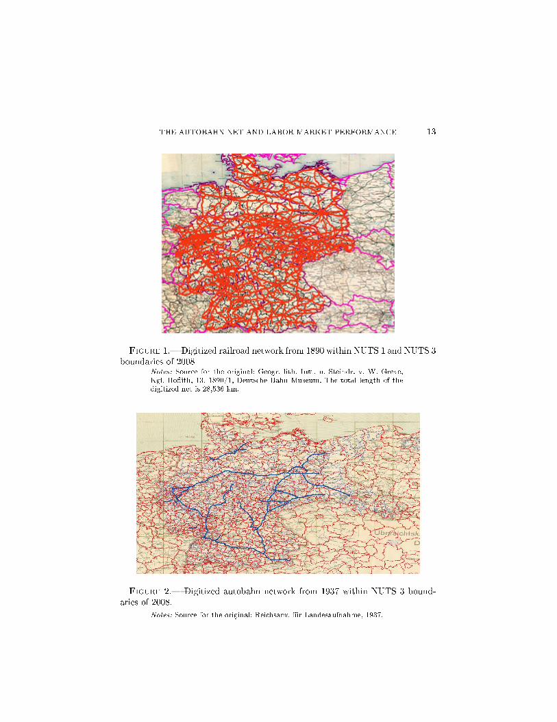
In the following, we make use of a plan of the German railroad network from1890. The plan was digitized within NUTS 1 and NUTS 3 boundaries of 2008(see Figure 1). The map shows that railway lines were planned according to abroad mixture of geographical conditions, the principle of federalism, and strate-gic economic and military aspects. The polycentric development is one of thebasic tenets of today's infrastructure and regional politics. In contrast to othercountries, such as France, the convergence of living conditions represents a ba-sic principle in the German constitution and has long been a focus of Germaneconomic policy (Aubert and Stephan (2000)).The exogeneity can be motivated by some historical facts. In 1870, Germany

consisted of a confederation of 39 states. Thus, in the beginning, a German na-tional railroad network (suggested by Friedrich List in 1833) could not be commu-nicated. However, the founding of the German Customs Union e�ected increasingtrade between the di�erent states. The bene�ts of this development were recog-nized, and the expansion of the transport system became desirable. Therefore,


the objective of building railroad lines was to connect cities and metropolitanareas as directly and practicably as possible to foster inter-regional trade in theshort term. However, neither later population and employment growth nor theincome development of modern cities were in the foreground of economic andinfrastructure politics. It is extremely unlikely that the economic developmentof the second half of the 20th century was anticipated at that time. A compar-ison with List's suggestions shows that his blueprints were partly modi�ed andgreatly expanded. The 1890 railroad network � 20 years after the creation of theBismarckian empire � was extended to the East by approximately 15,000 km.Some of these tracks were built to meet the requirements of expected economicgrowth at that time. However, an explicit intention to allow modern commutertra�c and goods exchange through low transport costs seems unlikely. The ini-tial railway building boom in Germany � mostly initiated by private companies �aimed for pro�ts in a not too distant future. For this reason, the plan of networkconstruction also shows the pro�tability of railroads at that time. If economicdevelopment phases are overshadowed by irrational acts of war, such as in thewars of 1864 (German-Danish), 1866 (Prussian-Austrian) and 1870-71 (German-French), long-term economic plans do not make sense. It is also clear that thenetwork of railroads had a military-strategic task, particularly with respect tothe national defense. A prominent example is the railroad line around Berlin. Thering in the east was completed in 1872, and the one in the west was completedin 1877.

4.1.2. The 1937 plan of the German autobahn system

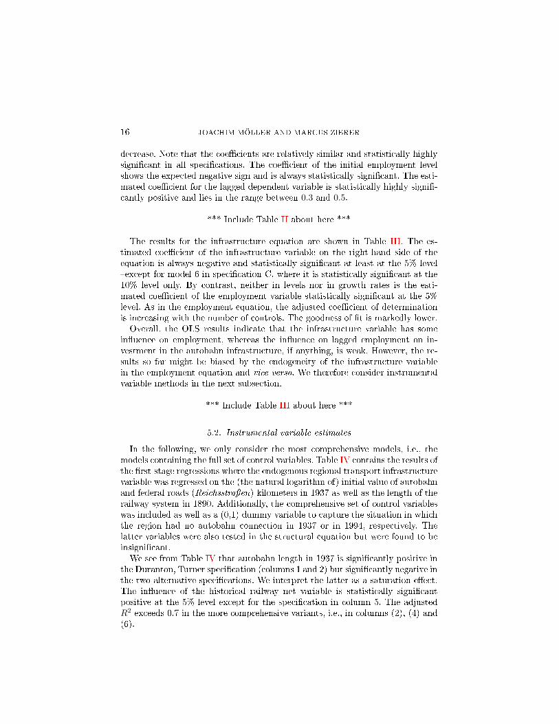
In the 1920s, north-south connections were planned and built. Initially, theHalle-Leipzig and Hamburg-Frankfurt-Basel sections were included in the auto-bahn construction programs. The expansion of the express highway network waslegally adopted in 1933. The 1937 autobahn network (see Figure 2) shows (i)roads that were already built and (ii) sections that should be completed in thefuture with the highest priority. The route length for the realized and plannedautobahn network amounted to more than 3,600 km in 1937. The 1937 plan hadan eminent in�uence on the current network of motorways. However, it seemsrather unlikely that the planned network concepts of that time anticipated thefuture regional labor market development, commuting and goods exchange ofthe post-war economy. Contemporaneous economic activity as well as strategicmilitary considerations clearly stood in the foreground. The latter is con�rmedby the so-called �Brown Memorandum� (submitted by Inspector General of RoadConstructions, Fritz Todt) (see Kornrumpf (1990)). The military-strategic im-portance of the autobahn network is demonstrated by the fact that it was ex-plicitly considered in the Four-Year Plan from fall 1936.


Figure 1.� Digitized railroad network from 1890 within NUTS 1 and NUTS 3boundaries of 2008

Notes: Source for the original: Geogr. lith. Inst. u. Steindr. v. W. Greve,Kgl. Ho�ith, 13. 1890/1, Deutsche Bahn Museum. The total length of thedigitized net is 28,536 km.

Figure 2.� Digitized autobahn network from 1937 within NUTS 3 bound-aries of 2008.

Notes: Source for the original: Reichsamt für Landesaufnahme, 1937.


4.2. Data and descriptive evidence

To obtain a consistent data set, we adjusted socio-demographic, economic andinfrastructure data in a adequate manner to the administrative territorial unitsat the NUTS 3 level of 2008. Historical infrastructure variables were obtainedfrom historical maps. These maps were digitized and transformed into a graphicalrepresentation. With the help of a geo-information system, the information couldbe mapped to the modern administrative units.

For the outcome variables, employment growth and the growth of the totalregional wage bill between 1994 and 2008 were chosen. We took 1994 as thestarting point of the analysis because the �rst years after re-uni�cation werecharacterized by extraordinary developments that a�ected population and em-ployment. Furthermore, the large migration processes in the initial period afterre-uni�cation might have biased the results. For the same reason, we decided toonly consider the time period before the Great Recession, which hit the Germanlabor market in 2009.

As further control variables, we used historical population data for the years1939, 1950, 1961 and 1970. Furthermore, the skill level of the work force mightplay a role in regional economic development. We therefore included the 1994share of intermediate and highly skilled workers generated from data of theInstitute for Employment Research (IAB). Moreover, we constructed seven (0,1)dummy variables as controls for (slightly aggregated) federal states (laender)and eight (0,1) dummy variables for types of regions ranging from metropolitancore cities to rural areas in the periphery.3

Table I presents some descriptive statistics for West German NUTS 3 re-gions. The average length and density of the autobahn net in the regions roughlyquadrupled from 1937 to 2008, with the major change occurring before 1994. In1937, 122 (37 percent) of regions at the NUTS 3 level had an autobahn withintheir area. This number increased to 291, or almost 90 percent, in 2008. However,there were still 35 regions without an autobahn running through their area atthe end of our observation period. The region with the highest density (Hof) hasalmost 1.3 km of autobahn length per square kilometer of its area.

*** Include Table I about here ***

5. ESTIMATION RESULTS

5.1. Speci�cation search and OLS results

Because our infrastructure variable, autobahn in kilometers(It), is equal to zerofor a number of regions, we use two alternative ways of calculating the relativechange. Both methods of calculating the growth rate led to similar results.

3The classi�cation is taken from the Bundesamt für Bauwesen, Städtebau und Raumordnungin Bonn.


The �rst way of handling the problem can be described as follows. We run aregression of ln It−1 on It for all cases where It−1 and It are strictly positive.Then, the non-de�ned values (ln 0) in period t−1 are replaced by the �tted valueof the regression. In an analogous way, a regression was run for the periods t andt+ 1 to replace the non-de�ned values in period t.The second method relies on a modi�ed growth rate:

(5.1)

%∆t−1,tIr =

{(Irt − Ir,t−1)/0.5(Irt + Ir,t−1)0

}if Irt+Ir,t−1

{> 0= 0

}.

Because this method creates an arti�cial mass point of the distribution at It = 2,we introduced a (0,1) dummy variable in the �rst-stage regression to capture thespeci�c situation of regions that in 1937 or 1994, respectively, had no autobahnwithin their area. In a variant of our estimation approach, only the �rst dummywas used.We used the OLS method to test for di�erent speci�cations of the basic equa-

tion relating the change in labor market performance to the infrastructure vari-able and other controls. Without presenting the test results in detail, the �ndingscan be summarized as follows:

� infrastructure variables are statistically highly signi�cant, but only whenintroduced with a time lag;

� the hypothesis that the coe�cients of the infrastructure variables add upto zero cannot be rejected; hence, a speci�cation in changes rather than inlevels is preferred;

� the same is true for the lagged population variables;� initial human capital variables matter for the labor market development ofthe regions;

� dummies for the region type and the federal states are jointly signi�cant;� the (log of) the region's area is statistically signi�cant in most speci�ca-tions;

� a measure of the relative change of the infrastructure variable clearly out-performs a qualitative variable that indicates whether the region is relatedto the autobahn net.

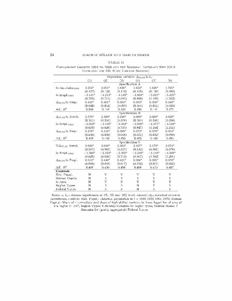
We �rst present OLS results for a regression of growth of regional employmenton infrastructure variables in the same speci�cation as in Duranton and Turner(2012) and compare them with our own speci�cation.Table II presents the outcome of OLS estimations of employment growth. The

comparison between the model of Duranton and Turner (2012) (Speci�cation A)and the two variants of our model (Speci�cation B for infrastructure measuredin log di�erences and Speci�cation C for infrastructure measured in modi�edgrowth rates) show qualitatively similar results. The adjusted coe�cient of de-termination increases markedly when more control variables are included. At thesame time, the estimated coe�cients of the core explanatory variables tend to


decrease. Note that the coe�cients are relatively similar and statistically highlysigni�cant in all speci�cations. The coe�cient of the initial employment levelshows the expected negative sign and is always statistically signi�cant. The esti-mated coe�cient for the lagged dependent variable is statistically highly signi�-cantly positive and lies in the range between 0.3 and 0.5.

*** Include Table II about here ***

The results for the infrastructure equation are shown in Table III. The es-timated coe�cient of the infrastructure variable on the right-hand side of theequation is always negative and statistically signi�cant at least at the 5% level�except for model 6 in speci�cation C, where it is statistically signi�cant at the10% level only. By contrast, neither in levels nor in growth rates is the esti-mated coe�cient of the employment variable statistically signi�cant at the 5%level. As in the employment equation, the adjusted coe�cient of determinationis increasing with the number of controls. The goodness of �t is markedly lower.Overall, the OLS results indicate that the infrastructure variable has some

in�uence on employment, whereas the in�uence on lagged employment on in-vestment in the autobahn infrastructure, if anything, is weak. However, the re-sults so far might be biased by the endogeneity of the infrastructure variablein the employment equation and vice versa. We therefore consider instrumentalvariable methods in the next subsection.

*** Include Table III about here ***

5.2. Instrumental variable estimates

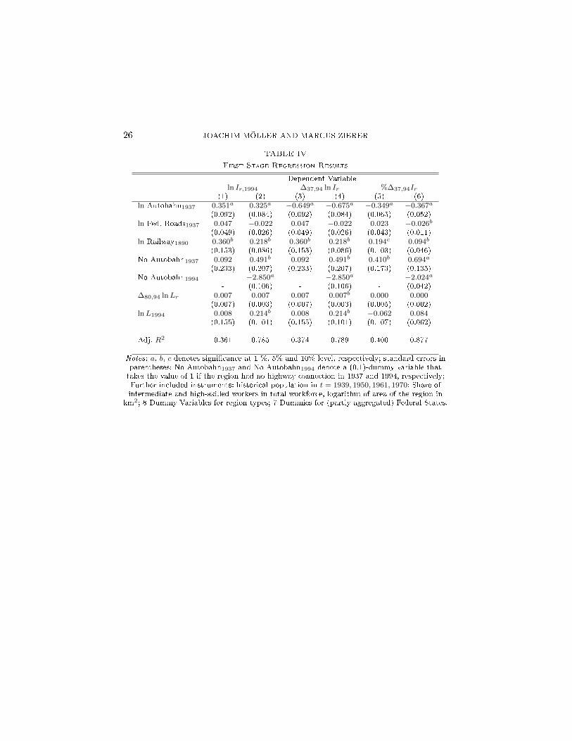
In the following, we only consider the most comprehensive models, i.e., themodels containing the full set of control variables. Table IV contains the results ofthe �rst-stage regressions where the endogenous regional transport infrastructurevariable was regressed on the (the natural logarithm of) initial value of autobahnand federal roads (Reichsstraÿen) kilometers in 1937 as well as the length of therailway system in 1890. Additionally, the comprehensive set of control variableswas included as well as a (0,1) dummy variable to capture the situation in whichthe region had no autobahn connection in 1937 or in 1994, respectively. Thelatter variables were also tested in the structural equation but were found to beinsigni�cant.We see from Table IV that autobahn length in 1937 is signi�cantly positive in

the Duranton, Turner speci�cation (columns 1 and 2) but signi�cantly negative inthe two alternative speci�cations. We interpret the latter as a saturation e�ect.The in�uence of the historical railway net variable is statistically signi�cantpositive at the 5% level except for the speci�cation in column 5. The adjustedR2 exceeds 0.7 in the more comprehensive variants, i.e., in columns (2), (4) and(6).


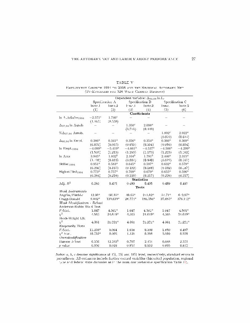
When considering the test statistics in the lower panel of Table V, it appearsthat the variants with the extended set of instruments (Instr.2) are clearly prefer-able. Although the Angrist-Pischke and the Cragg-Donald test statistics supportthe relevance of the instruments in all cases, the null in the robust weak iden-ti�cation tests cannot be rejected in all speci�cations using the restricted setof instruments (Instr.1). Moreover, speci�cation A appears to be problematic inboth variants. Identi�cation is weak when using the restricted set of instruments,whereas in the estimates using the extended set of instruments, the Hanson testrejects the hypothesis that the instruments are uncorrelated with the residuals.Hence, we conclude that speci�cations B and C are more suitable.With regard to the estimated coe�cients, one can observe that the coe�cient of

the autobahn variable is higher when the extended set of instruments is used. Inthe preferred variant, the estimated coe�cient is roughly 2 in speci�cation B androughly 3 in speci�cation C. Both estimates are statistically highly signi�cant.The coe�cient of the lagged endogenous variable is highly signi�cantly negative,whereas the coe�cient of the lagged growth rate of employment is positive,indicating some sluggishness in the process of adjusting regional employment.The human capital variables are also highly statistically signi�cant and all carrya positive sign. Hence, regions with more human capital per employee in theinitial period had better performance thereafter.Interestingly, we �nd evidence for a correlation between the explanatory in-

frastructure variable and the disturbance term only in the model in column (1),which we disregard for other reasons. The null of exogeneity of the autobahnvariable cannot be rejected in all variants of the model shown in columns (2)to (6). Hence, it would be justi�ed to return to the OLS results because theseestimates are more e�cient.

*** Include Table IV about here ***

*** Include Table V about here ***

5.3. Results for the impact of the regional autobahn net on the wage bill

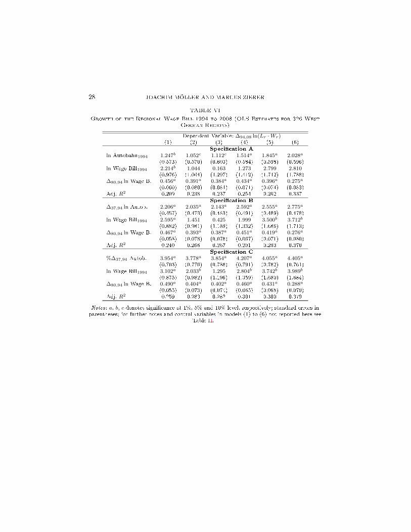
The e�ects of the growth in transport infrastructure � as measured by auto-bahn kilometers � on the total regional wage bill are estimated in an analogousway as described in the last two subsections. Table VI presents the results forthe OLS speci�cations. In contrast to the �ndings for the employment growthvariable, the estimated coe�cient for the autobahn variable tends to increase inall speci�cations when more control variables are introduced.The coe�cient of infrastructure is always positive. It is statistically highly

signi�cant in all variants of speci�cations B and C, whereas this is the case onlyin the models with a more comprehensive set of control variables in speci�cationA. In the preferred models in column (6), the coe�cient of the infrastructure


variable on regional wage bill growth lies in the range between 2.0 (speci�cationA) and 4.4 (speci�cation C). It is somewhat puzzling that the coe�cient ofthe lagged regional wage bill is positive in all variants. This �nding indicatesdivergence of the total regional wage bill distribution. The choice of other controlvariables has a relatively small in�uence on the results.Again, the IV approach passes all relevant test statistics. The instruments are

powerful, and there is no indication that the residuals are correlated with theinstruments. The impact of the growth in autobahn kilometers on the wage billis estimated to be between 0.38 and 0.51. According to our analysis, the causale�ect of infrastructure on the regional wage bill is in the order of magnitude of0.47. This result implies that an increase in the autobahn length of one standarddeviation led to an additional increase in the regional wage bill of roughly 2.3percentage points in the 1994-2008 period. The e�ect obtained from the IV esti-mation is approximately 60% smaller than the OLS estimate. However, it is stillstatistically highly signi�cant.A comparison of results for our two basic variants of the estimation indicate

that the e�ect of infrastructure on regional employment performance tends tobe higher than that for employment growth. As argued in the theoretical part ofthe paper, this must be expected because the e�ect of infrastructure on wages ispositive.

*** Include Table VI about here ***

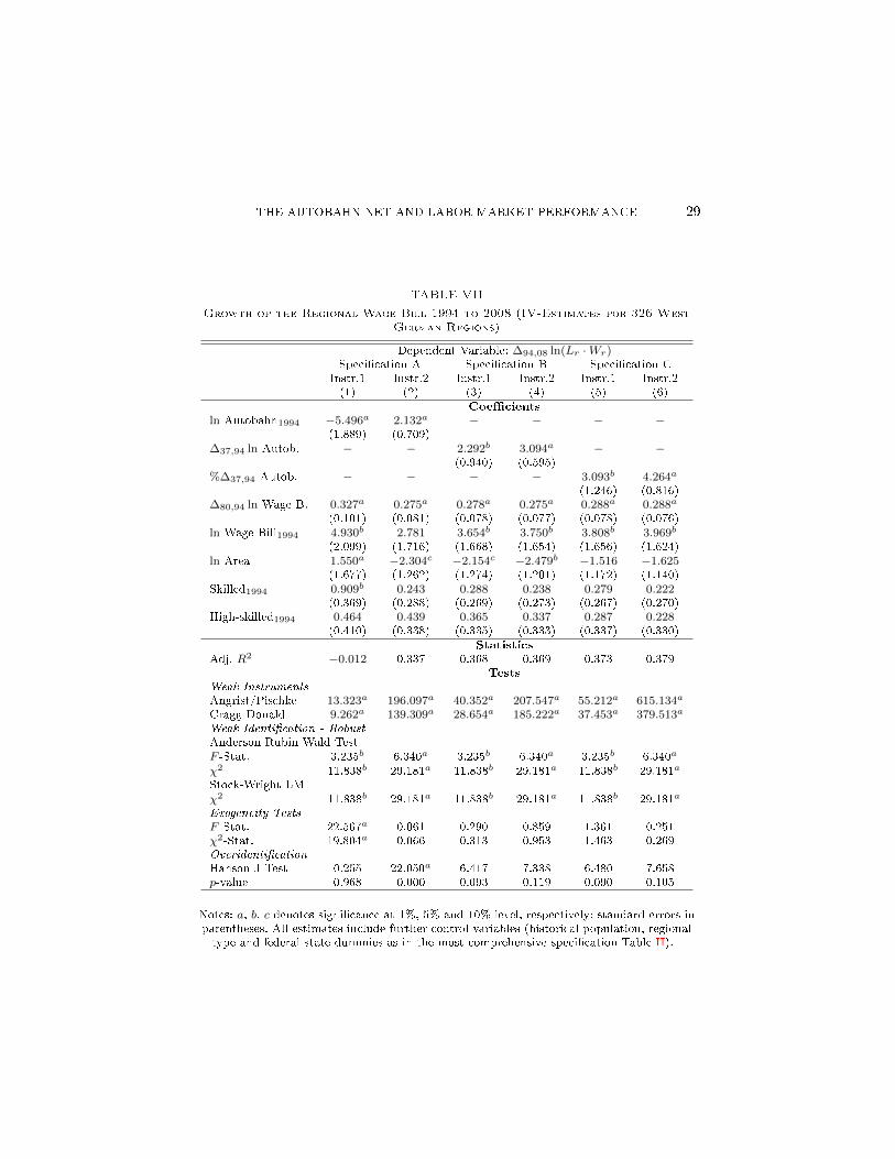
We also ran IV regressions using the same two sets of instruments as in theestimates for regional employment growth. Table VII contains the results, whichare qualitatively similar to those for employment growth. Again, the identi�-cation is stronger according to the Anderson-Rubin and the Stock-Wright testswhen the extended set of control is used. Speci�cation A yields a negative R2 anda negative sign for the infrastructure variable in column (1). The variant in col-umn (2), however, seems to violate the uncorrelatedness condition. Speci�cationsB and C perform better, and the instruments appear stronger in both variants.The over-identi�cation test does not reject uncorrelatedness, at least when usingthe extended set of instruments. Speci�cation C in this variant yields the highestcoe�cient of determination and seems to be the preferable model (column (6)).As in the OLS estimates, the dependent variable in levels has a positive sign.The lagged dependent variable exhibits a statistically highly signi�cant positivecoe�cient, indicating some sluggishness in the development of the regional wagebill. Note that the human capital variables do not seem to have an importantin�uence.In addition to the OLS and 2SLS estimates, we used a robust GMM and LIML

estimator. As the overview in Table VIII shows, the di�erent estimators yieldsimilar results. With the estimated coe�cients, we calculated the impact of aone standard deviation increase of the autobahn variable on the growth of re-gional employment and the total wage bill. Several points must be mentioned.


The di�erences between speci�cations B and C are small. With the extendedset of instruments, all coe�cients are positive, statistically highly signi�cant andvery close to the OLS results. Furthermore, for the restricted set of instruments,we �nd positive and signi�cant e�ects that are somewhat lower than the OLSestimates. Depending on the speci�cation or the estimation method, one stan-dard deviation of the infrastructure variable leads to higher regional employmentgrowth of between 1.8 and 3 percentage points in the 1994 to 2008 period. Thecorresponding impact on the total regional wage bill is between 2.7 and 4.3 per-centage points. The higher e�ect for the total wage bill implies that an increasein the regional autobahn net led not only to more employment but also to higherwages.

*** Include Table VII about here ***

*** Include Table VIII about here ***

6. CONCLUSIONS

This paper investigates a causal e�ect of investment in transport infrastruc-ture � particularly in the autobahn net � on regional labor market performance.We �rst present a theoretical model in the spirit of New Economic Geographythat explicitly includes regional heterogeneity with respect to transport infra-structure. We argue that in addition to a direct e�ect on the transportation of�nal goods and corresponding market potential e�ects, there are positive e�ectsof the regional transport system on the e�ciency of production.The theoretical reasoning leads to a highly interdependent non-linear model

that cannot be estimated directly. However, the model is able to clarify the di�er-ent channels by which transport costs are related to labor market performance.It is important to note that the theoretical model is ambiguous with respectto the impact of transport infrastructure on regional labor market performance.Hence, empirical analysis is required.We concentrate on a speci�c part of the German transport infrastructure, the

autobahn net. An autobahn connection leads to a considerable increase in theaccessibility of the region and lower transport costs. Speci�cation tests suggestthat changes in the autobahn net a�ect regional labor market performance onlywith a time lag. Moreover, it seems that changes in regional employment or thetotal regional wage bill are related to changes in transport infrastructure, not itslevel.In the regression analysis, a crucial problem is the possible endogeneity of

transport infrastructure investments. Hence, a region might be chosen to obtainan autobahn connection if it is expected to become an economically successfularea in the future. To address the endogeneity issue, we rely on a strategy withhistorical instrumental variables. These are taken from historical plans for auto-


bahns and railway tracks and were digitized and related to the NUTS 3 areas oftoday.The instrumental variable approach turns out to be successful. According to

the corresponding test statistics, we can show that in our preferred speci�cations,the instruments are relevant and uncorrelated with the residuals. Moreover, thestrategy allows us to test for the exogeneity of the autobahn variable in the em-ployment and wage bill equations. According to the test statistics, exogeneitycannot be rejected in our preferred speci�cation variants. This �nding is sup-ported by the small di�erences between the OLS and the IV estimates.According to our estimates, an increase in autobahn length of one standard

deviation in the 1937 to 1994 period leads to higher employment growth between1.8 and 3 percentage points and to higher total growth of the wage bill between2.7 and 4.3 percentage points in the 1994 to 2008 period. We therefore concludethat higher accessibility and lower transport costs through a more extensiveautobahn net are bene�cial to the regional labor market performance.


REFERENCES

Anas, Alex, �The estimation of multinomial Logit models of joint location and mode choicefrom aggregated data.,� Journal of Regional Science, 1981, 21, 223�242.

, Residential Location Markets and Urban Transportation: Economic Theory, Econo-

metrics and Policy Analysis with Discrete Choice Models, Oxford: Academic Press., 1982.and Liang Shyong Duann, �Dynamic forecasting of travel demand, residential

location and land development,� Papers of the Regional Science Association, 1985, 56 (1),37�58.

Aschauer, David Alan, �Is public expenditure productive?,� Journal of Monetary Eco-

nomics, March 1989, 23 (2), 177�200.Aubert, S. and A. Stephan, �Regionale Infrastrukturpolitik und ihre Auswirkung auf die

Produktivität: Ein Vergleich von Deutschland und Frankreich,� Discussion Papers, Wis-senschaftszentrum Berlin für Sozialforschung, Deutsches Institut für Wirtschaftsforschung2000.

Baum-Snow, Nathaniel, �Did highways cause suburbanization?,� The Quarterly Journal ofEconomics, 2007, 122 (2), 775�805.

BBSR, �Stadtansichten: Befunde der BBSR-Umfrage aus Groÿ- und Mittelstädten,� July 2011.Bougheas, Spiros, Panicos O Demetriades, and Theofanis P Mamuneas, �Infrastruc-

ture, specialization, and economic growth,� Canadian Journal of Economics, 2000, 33 (2),506�522.

Brakman, Steven, Harry Garretsen, and Charles van Marrewijk, The New Introduc-

tion to Geographical Economics number 9780521875325. In `Cambridge Books.', CambridgeUniversity Press, April 2009.

Brülhart, Marius and Federica Sbergami, �Agglomeration and growth: Cross-countryevidence,� Journal of Urban Economics, 2009, 65 (1), 48�63.

Calderon, César and Luis Servén, �The output cost of Latin America's infrastructuregap,� in William Easterly and Luis Serven, eds., The Limits of Stabilization: Infrastructure,Public De�cits, and Growth in Latin America, Stanford University Press, 2003, pp. 95�118.

Canning, David and Peter Pedroni, �The e�ect of infrastructure on long run economicgrowth,� 2004.

Duranton, Gilles and Matthew A Turner, �Urban growth and transportation,� The Re-view of Economic Studies, 2012, 79 (4), 1407�1440.

Ford, Robert and Pierre Poret, Infrastructure and private-sector productivity number 91.In `Working Paper - Economic Series.', OECD Paris, 1991.

Frey, René Leo, Die Infrastruktur als Mittel der Regionalpolitik: Eine wirtschaftstheoretis-

che Untersuchung zur Bedeutung der Infrastrukturförderung von entwicklungsschwachen

Regionen in der Schweiz, Vol. 1 of Publikationen des Schweizerischen Nationalfonds aus

den Nationalen Forschungsprogrammen, Bern: Haupt, 1979.Fujita, Masahisa, Paul R. Krugman, and Anthony Venables, The Spatial Economy:

Cities, Regions and International trade, Cambridge and Mass: MIT Press, 1999.Gramlich, Edward M, �Infrastructure investment: A review essay,� Journal of Economic

Literature, 1994, 32 (3), 1176�1196.Hanson, Gordon H., �Market potential, increasing returns and geographic concentration,�

Journal of International Economics, 2005, 67 (1), 1�24.Harris, C. D., �The market as a factor in the localization of industry in the United States,�

Annals of the Association of American Geographers, 1954, 44, 315�348.Holtz-Eakin, D., �Private Output, Government Capital, And The Infrastructure Crisis,�

Discussion Papers 1988-08, Columbia University, Department of Economics 1988.Hsiao, Cheng and Yan Shen, �Foreign Direct Investment and Economic Growth: The Im-

portance of Institutions and Urbanization*,� Economic Development and Cultural Change,2003, 51 (4), 883�896.

Kornrumpf, M., HAFRABA e. V., Deutsche Autobahn-Planung 1926-1934. 1990.McDonald, J. F. and C. I. Osuji, �The e�ect of anticipated transportation improvement

on residential land values,� Regional Science and Urban Economics, 1995, 25 (3), 261�278.


McMillen, Daniel P. and John F. McDonald, �Suburban Subcenters and EmploymentDensity in Metropolitan Chicago,� Journal of Urban Economics, March 1998, 43 (2), 157�180.

Munnell, Alicia H., �Why has productivity growth declined? Productivity and public in-vestment,� New England Economic Review, Jan 1990, 30, 3�22.

Steen, Robert C, �Nonubiquitous transportation and urban population density gradients,�Journal of Urban Economics, 1986, 20 (1), 97�106.

Thünen, Johann H. Von, Der isolirte Staat in Beziehung auf Landwirthschaft und Nation-

alökonomie, neu hrsg. von Walter Braeuer u. Eberhard E. A. Gerhardt 1966 ed. 1842.


TABLE I

Descriptive Statistics for the Development of Transport Infrastructure ofWest German NUTS-3-Regions

Autobahn Net1937 1994 2008

Total number of regions 326Area in km2

- Average 761.52- St.deviation 534.05- Minimum 35.71- Maximum 2881.40Regions without autobahn 204 44 35Regions with autobahn 122 282 291Highway length in km- Average 6.84 29.83 30.38- St.deviation 11.81 27.11 24.83- Minimum 0 0 0- Maximum 52.92 164.00 111.59Highway density- Average 1.72 6.83 6.75- St.deviation 5.39 9.54 9.23- Maximum 83.86 90.49 128.22

Railway Net1890 1994 2008

Regions with railroads 326 326 326Railway net length in km- Average 58.87 93.83 87.61- St.deviation 37.19 56.28 52.55- Minimum 3.83 3.86 3.86- Maximum 52.92 164.00 111.59Railway density- Average 120.96 181.92 170.24- St.deviation 115.58 158.28 144.33- Minimum 7.34 13.43 13.43- Maximum 1428.60 1907.00 1735.43

Notes: Highway (railway) density is calculated as autobahn (railway) length in km per 100km2.


TABLE II

Employment Growth 1994 to 2008 and the Regional Autobahn Net (OLSEstimates for 326 West German Regions)

Dependent variable: ∆94,08 lnLr

(1) (2) (3) (4) (5) (6)Speci�cation A

ln Autobahn1994 2.252a 2.051a 1.826a 1.622a 1.626a 1.765a

(0.447) (0.422) (0.413) (0.415) (0.438) (0.460)ln Empl.1994 −3.141a −4.213a −4.149a −4.804a −5.021a −5.425a

(0.733) (0.715) (0.835) (0.890) (1.109) (1.262)∆80,94 ln Empl. 0.443a 0.401a 0.384a 0.353a 0.356a 0.340a

(0.040) (0.054) (0.052) (0.054) (0.055) (0.059)Adj. R2 0.369 0.418 0.428 0.436 0.441 0.475

Speci�cation B∆37,94 ln Autob. 2.578a 2.389a 2.238a 2.080a 2.068a 2.028a

(0.357) (0.350) (0.324) (0.334) (0.348) (0.358)ln Empl.1994 −2.059a −3.150a −3.334a −3.939a −4.371a −4.549a

(0.620) (0.626) (0.735) (0.847) (1.104) (1.211)∆80,94 ln Empl. 0.478a 0.418a 0.399a 0.373a 0.379a 0.354a

(0.039) (0.050) (0.048) (0.051) (0.052) (0.056)Adj. R2 0.405 0.449 0.459 0.463 0.469 0.495

Speci�cation C%∆37,94 Autob. 3.926a 3.649a 3.363a 3.167a 3.179a 3.074a

(0.557) (0.565) (0.527) (0.532) (0.561) (0.576)ln Empl.1994 −1.360a −2.433a −2.402a −3.248a −4.118a −4.269a

(0.625) (0.636) (0.743) (0.867) (1.102) (1.201)∆80,94 ln Empl. 0.513a 0.440a 0.421a 0.386a 0.395a 0.370a

(0.039) (0.048) (0.047) (0.050) (0.051) (0.056)Adj. R2 0.408 0.450 0.458 0.466 0.473 0.497Controls

Hist. Popul. N Y Y Y Y YHuman Capital N N Y Y Y Yln Area N N N Y Y YRegion Types N N N N Y YFederal States N N N N N Y

Notes: a, b, c denotes signi�cance at 1%, 5% and 10% level, respectively; standard errors inparentheses; controls: Hist. Popul.: historical population in t = 1939, 1950, 1961, 1970; HumanCapital: Share of intermediate and share of high-skilled workers; ln Area: logarithm of area of

the region in km2; Region Types: 8 dummy-Variables for region types; Federal States: 7dummies for (partly aggregated) Federal States.


TABLE III

Growth of the Autobahn Net 1994 to 2008 (OLS Estimates for 326 WestGerman Regions)

Dependent variable: ∆94,08 ln Ir(1) (2) (3) (4) (5) (6)

Speci�cation Aln Autobahn1994 −0.115a −0.115a −0.109a −0.117a −0.119a −0.114a

(0.033) (0.033) (0.031) (0.034) (0.034) (0.034)ln Empl.1994 −0.035 −0.012 0.033 0.013 0.021 0.092c

(0.028) (0.033) (0.039) (0.036) (0.048) (0.051)Adj. R2 0.102 0.107 0.126 0.129 0.142 0.196

Speci�cation B∆37,94 ln Autobahn −0.089a −0.084a −0.079a −0.082a −0.076a −0.070a

(0.026) (0.024) (0.023) (0.025) (0.025) (0.024)∆94,08 ln Empl. −0.001 0.002 0.003 0.003 0.002 −0.003

(0.004) (0.004) (0.003) (0.003) (0.004) (0.004)Adj. R2 0.048 0.059 0.094 0.092 0.104 0.166

Speci�cation C%∆37,94 Autobahn −0.084b −0.081b −0.073b −0.072b −0.070b −0.062c

(0.037) (0.036) (0.035) (0.035) (0.035) (0.035)∆94,08 ln Empl. 0.001 0.003 0.004 0.004 0.003 −0.001

(0.003) (0.003) (0.003) (0.003) (0.003) (0.003)Adj. R2 0.023 0.045 0.073 0.071 0.088 0.159

Notes: a, b, c denotes signi�cance at 1%, 5% and 10% level, respectively; standard errors inparentheses; for further notes and control variables in models (1) to (6), see Table II.


TABLE IV

First-Stage Regression Results

Dependent Variableln Ir,1994 ∆37,94 ln Ir %∆37,94Ir

(1) (2) (3) (4) (5) (6)ln Autobahn1937 0.351a 0.325a −0.649a −0.675a −0.349a −0.367a

(0.092) (0.084) (0.092) (0.084) (0.065) (0.052)ln Fed. Roads1937 0.047 −0.022 0.047 −0.022 0.023 −0.026b

(0.049) (0.026) (0.049) (0.026) (0.043) (0.011)ln Railway1890 0.360b 0.218b 0.360b 0.218b 0.194c 0.094b

(0.153) (0.086) (0.153) (0.086) (0.103) (0.046)No Autobahn1937 0.092 0.491b 0.092 0.491b 0.410b 0.694a

(0.233) (0.207) (0.233) (0.207) (0.173) (0.135)No Autobahn1994 - −2.850a - −2.850a - −2.024a

- (0.106) - (0.106) - (0.042)∆80,94 lnLr 0.007 0.007 0.007 0.007b 0.000 0.000

(0.007) (0.003) (0.007) (0.003) (0.005) (0.002)lnL1994 0.008 0.214b 0.008 0.214b −0.062 0.084

(0.155) (0.101) (0.155) (0.101) (0.107) (0.062)

Adj. R2 0.361 0.785 0.374 0.789 0.400 0.877

Notes: a, b, c denotes signi�cance at 1 %, 5% and 10% level, respectively; standard errors inparentheses; No Autobahn1937 and No Autobahn1994 denote a (0,1)-dummy variable thattakes the value of 1 if the region had no highway connection in 1937 and 1994, respectively;Further included instruments: historical population in t = 1939, 1950, 1961, 1970; Share ofintermediate and high-skilled workers in total workforce, logarithm of area of the region in

km2; 8 Dummy Variables for region types; 7 Dummies for (partly aggregated) Federal States.


TABLE V

Employment Growth 1994 to 2008 and the Regional Autobahn Net(IV-Estimates for 326 West German Regions)

Dependent variable: ∆94,08 lnLr

Speci�cation A Speci�cation B Speci�cation CInstr.1 Instr.2 Instr.1 Instr.2 Instr.1 Instr.2(1) (2) (3) (4) (5) (6)

Coe�cients

ln Autobahn1994 −2.571c 1.746c − − − −(1.465) (0.550)

∆37,94 ln Autob. − − 1.350c 2.098a − −(0.710) (0.443)

%∆37,94 Autob. − − − − 1.892c 2.922a

(0.970) (0.614)∆80,94 ln Empl. 0.386a 0.341a 0.356a 0.354a 0.366a 0.369a

(0.070) (0.057) (0.055) (0.054) (0.056) (0.054)ln Empl.1994 −4.099a −5.419a −4.661a −4.537a −4.506a −4.299a

(1.535) (1.213) (1.205) (1.173) (1.225) (1.162)ln Area 3.945a 1.832b 2.104b 1.781b 2.446a 2.315a

(1.128) (0.893) (0.907) (0.840) (0.822) (0.787)Skilled1994 0.951a 0.583a 0.645a 0.597a 0.632a 0.578a

(0.260) (0.197) (0.192) (0.188) (0.192) (0.187)High-skilled1994 0.773a 0.757a 0.709a 0.679a 0.655a 0.596a

(0.264) (0.216) (0.220) (0.217) (0.226) (0.217)Statistics

Adj. R2 0.285 0.475 0.489 0.495 0.489 0.497Tests

Weak Instruments

Angrist/Pischke 12.90a 196.35a 40.65a 211.02a 54.71a 612.97a

Cragg-Donald 9.042a 139.639a 28.774a 186.556a 37.085a 376.142a

Weak Identi�cation - Robust

Anderson-Rubin Wald TestF -Stat. 1.047 4.501a 1.047 4.501a 1.047 4.501a

χ2 4.565 24.619a 4.565 24.619a 4.565 24.619a

Stock-Wright LMχ2 4.361 21.221a 4.361 21.221a 4.361 21.221a

Exogeneity Tests

F -Stat. 11.259a 0.004 1.038 0.090 1.850 0.497χ2-Stat. 10.732a 0.005 1.128 0.098 2.009 0.529Overidenti�cation

Hanson J-Test 0.350 12.243b 0.767 2.454 0.608 2.351p-value 0.950 0.016 0.857 0.653 0.895 0.672

Notes: a, b, c denotes signi�cance at 1%, 5% and 10% level, respectively; standard errors inparentheses. All estimates include further control variables (historical population, regionaltype and federal state dummies as in the most comprehensive speci�cation Table II).


TABLE VI

Growth of the Regional Wage Bill 1994 to 2008 (OLS Estimates for 326 WestGerman Regions)

Dependent Variable: ∆94,08 ln(Lr ·Wr)(1) (2) (3) (4) (5) (6)

Speci�cation A

ln Autobahn1994 1.247b 1.052c 1.112c 1.514a 1.845a 2.028a

(0.573) (0.570) (0.603) (0.584) (0.598) (0.596)ln Wage Bill1994 2.214b 1.044 0.163 1.273 2.799 2.810

(0.976) (1.064) (1.297) (1.412) (1.712) (1.788)∆80,94 ln Wage B. 0.456a 0.391a 0.384a 0.434a 0.396a 0.275a

(0.060) (0.080) (0.081) (0.071) (0.074) (0.083)Adj. R2 0.209 0.238 0.237 0.254 0.262 0.337

Speci�cation B

∆37,94 ln Autob. 2.206a 2.035a 2.143a 2.592a 2.555a 2.775a

(0.457) (0.473) (0.483) (0.491) (0.489) (0.478)ln Wage Bill1994 2.595a 1.451 0.425 1.999 3.500b 3.712b

(0.882) (0.981) (1.189) (1.332) (1.686) (1.713)∆80,94 ln Wage B. 0.467a 0.393a 0.387a 0.451a 0.419a 0.276a

(0.058) (0.078) (0.078) (0.067) (0.071) (0.080)Adj. R2 0.240 0.266 0.267 0.291 0.293 0.370

Speci�cation C

%∆37,94 Autob. 3.954a 3.778a 3.854a 4.207a 4.055a 4.405a

(0.703) (0.776) (0.788) (0.791) (0.782) (0.761)ln Wage Bill1994 3.102a 2.033b 1.295 2.804b 3.742b 3.989b

(0.875) (0.982) (1.196) (1.359) (1.680) (1.684)∆80,94 ln Wage B. 0.490a 0.404a 0.402a 0.460a 0.431a 0.288a

(0.055) (0.073) (0.074) (0.065) (0.068) (0.079)Adj. R2 0.259 0.283 0.282 0.301 0.300 0.379

Notes: a, b, c denotes signi�cance at 1%, 5% and 10% level, respectively; standard errors inparentheses; for further notes and control variables in models (1) to (6) not reported here see

Table II.


TABLE VII

Growth of the Regional Wage Bill 1994 to 2008 (IV-Estimates for 326 WestGerman Regions)

Dependent Variable: ∆94,08 ln(Lr ·Wr)Speci�cation A Speci�cation B Speci�cation C

Instr.1 Instr.2 Instr.1 Instr.2 Instr.1 Instr.2(1) (2) (3) (4) (5) (6)

Coe�cients

ln Autobahn1994 −5.496a 2.132a − − − −(1.889) (0.709)

∆37,94 ln Autob. − − 2.292b 3.094a − −(0.940) (0.595)

%∆37,94 Autob. − − − − 3.093b 4.264a

(1.246) (0.816)∆80,94 ln Wage B. 0.327a 0.275a 0.278a 0.275a 0.288a 0.288a

(0.101) (0.081) (0.078) (0.077) (0.078) (0.076)ln Wage Bill1994 4.930b 2.781 3.654b 3.750b 3.808b 3.969b

(2.099) (1.716) (1.668) (1.654) (1.656) (1.624)ln Area 1.550a −2.304c −2.154c −2.479b −1.516 −1.625

(1.677) (1.262) (1.274) (1.201) (1.172) (1.140)Skilled1994 0.909b 0.243 0.288 0.238 0.279 0.222

(0.369) (0.288) (0.269) (0.273) (0.267) (0.270)High-skilled1994 0.464 0.439 0.365 0.337 0.287 0.228

(0.410) (0.338) (0.335) (0.333) (0.337) (0.330)Statistics

Adj. R2 −0.012 0.337 0.368 0.369 0.373 0.379Tests

Weak Instruments

Angrist/Pischke 13.323a 196.097a 40.352a 207.547a 55.212a 615.134a

Cragg-Donald 9.262a 139.309a 28.654a 185.222a 37.453a 379.513a

Weak Identi�cation - Robust

Anderson-Rubin Wald TestF -Stat. 3.235b 6.340a 3.235b 6.340a 3.235b 6.340a

χ2 11.838b 29.181a 11.838b 29.181a 11.838b 29.181a

Stock-Wright LMχ2 11.838b 29.181a 11.838b 29.181a 11.838b 29.181a

Exogeneity Tests

F -Stat. 22.567a 0.061 0.290 0.859 1.361 0.251χ2-Stat. 19.804a 0.066 0.313 0.953 1.463 0.269Overidenti�cation

Hanson J-Test 0.255 22.050a 6.417 7.338 6.480 7.658p-value 0.968 0.000 0.093 0.119 0.090 0.105

Notes: a, b, c denotes signi�cance at 1%, 5% and 10% level, respectively; standard errors inparentheses. All estimates include further control variables (historical population, regionaltype and federal state dummies as in the most comprehensive speci�cation Table II).


TABLE VIII

The Impact of Regional Transport Infrastructure on Regional Employment andthe Wage Bill for Different Estimation Methods

A. Employment Growth

Instruments 1 Instruments 2Method Coe�. z-Stat. Impact Coe�. z-Stat. Impact

Speci�cation AOLS 1.765 3.836 2.421 1.765 3.836 2.4212SLS − − − 1.746 3.661 2.395GMM-rob. − − − 1.853 3.387 2.541LIML-rob. − − − 1.744 3.105 2.393

Speci�cation BOLS 2.028 5.664 2.829 2.028 5.664 2.8292SLS 1.350 2.010 1.884 2.098 5.185 2.927GMM-rob. 1.356 1.923 1.892 2.077 4.705 2.897LIML-rob. 1.341 1.871 1.871 2.099 4.719 2.928

Speci�cation COLS 3.074 5.333 2.982 3.074 5.333 2.9822SLS 1.892 2.076 1.835 2.922 5.212 2.833GMM-rob. 1.917 1.987 1.859 2.911 4.760 2.823LIML-rob. 1.882 1.929 1.825 2.920 4.749 2.832

B. Wage Bill

Instruments 1 Instruments 2Method Coe�. z-Stat. Impact Coe�. z-Stat. Impact

Speci�cation AOLS 2.028 3.401 2.783 2.028 3.401 2.7832SLS − − − 2.132 3.108 2.925GMM-rob. − − − 2.040 2.889 2.798LIML-rob. − − − 2.144 2.925 2.942

Speci�cation BOLS 2.775 5.809 3.872 2.775 5.809 3.8722SLS 2.292 2.388 3.197 3.094 5.331 4.316GMM-rob. 2.274 2.474 3.173 3.015 5.088 4.206LIML-rob. 2.262 2.306 3.156 3.102 5.182 4.328

Speci�cation COLS 4.405 5.788 4.272 4.405 5.788 4.2722SLS 3.093 2.401 2.999 4.264 5.351 4.135GMM-rob. 3.121 2.541 3.027 4.172 5.135 4.046LIML-rob. 3.026 2.349 2.935 4.261 5.207 4.132

Notes: TSLS : 2-Stage Least Squares, GMM-rob.: Generalized Method of Moments, estimatese�cient for arbitrary heteroskedasticity and statistics robust to heteroskedasticity;LIML-rob.: Limited Maximum Likelihood Estimator, estimates e�cient for arbitrary

heteroskedasticity and statistics robust to heteroskedasticity; �Impact� is the e�ect of a onestandard deviation increase of the respective endogenous infrastructure variable; Instruments1 (2): speci�cation excluding (including) a (0,1)-dummy variable for no autobahn in 1994.

the impact of the german autobahn net on regional labor market...

Documents