UMR DIAL 225 Place du Maréchal de Lattre de Tassigny 75775 • Paris Cedex 16 •Tél. (33) 01 44 05 45 42 • Fax (33) 01 44 05 45 45

• 4, rue d’Enghien • 75010 Paris • Tél. (33) 01 53 24 14 50 • Fax (33) 01 53 24 14 51 E-mail : dial@dial.prd.fr • Site : www.dial.prd.fr

DOCUMENT DE TRAVAIL DT/2010-04

The impact of trade openness on regional inequality : the cases of India and Brazil

Marie DAUMAL

THE IMPACT OF TRADE OPENNESS ON REGIONAL INEQUALITY : THE CASES OF INDIA AND BRAZIL1

Marie Daumal Université Paris 8 Vincennes-Saint-Denis

Université Paris-Dauphine, LEDa, UMR DIAL marie.daumal@univ-paris8.fr

Document de travail UMR DIAL Février 2010

Abstract

Regional inequalities are large in India and Brazil and represent a development challenge. This paper aims to determine whether regional disparities are linked to countries’ trade openness. An annual indicator of regional inequalities is constructed for India over the period 1980-2003 and for Brazil over 1985-2003. Results from time series regressions show that Brazil’s trade openness contributes to the reduction in regional inequalities in Brazil. The opposite result is found for India. India’s trade openness is an important factor aggravating income inequality among Indian states. In both countries, the inflows of foreign direct investment are found to increase regional disparities.

Key words : Trade openness, regional inequality, India, Brazil, time series regression.

Résumé

Dans les années 90, les inégalités régionales ont fortement augment´e en Inde. Les inégalités entre Etats brésiliens sont importantes et constituent un problème politique majeur pour la fédération brésilienne. En 1991, ces deux pays se sont progressivement ouverts au commerce international. L’objectif du papier est de déterminer s’il existe ou non un lien entre les inégalités régionales et l’ouverture commerciale dans les cas de l’Inde et du Brésil. J’ai construit un indicateur, l’index Gini, qui est une mesure des inégalités régionales, sur la période 1980-2004 pour l’Inde et sur la période 1985-2004 pour le Brésil. Cet indicateur des inégalités régionales est ensuite régressé sur divers déterminants dont l’ouverture commerciale des pays, en utilisant la technique des séries temporelles et des modèles vectoriels à correction d’erreur. Je trouve que l’ouverture commerciale de l’Inde a fortement aggravé les inégalités existant entre l’Inde du Nord, de plus en plus pauvre, et l’Inde du Sud de plus en plus riche. Or ces inégalités régionales croissantes sont maintenant une source de tension et de conflits au sein de la fédération indienne, les Etats du Sud ne voulant plus “payer” pour le Nord du pays. Au contraire, l’ouverture du Brésil semble avoir entraîné une diminution des inégalités entre Etats brésiliens.

Mots clés : Ouverture commerciale, inégalités régionales, Inde, Brésil, séries temporelles.

JEL Classification : F43, R11

1 Many thanks to Jean-Marc Siroën, Christophe Hurlin, Sandra Poncet, Philippe De Vreyer, Jean-François Jacques for their help and the

participants of the ETSG conference in Warsaw (2008).

1 Introduction

Regional inequalities, namely per capita income inequalities across states, are a matter of serious

concern in India and in Brazil. Regional disparity has been rising in India since the 1990s and

now reachs a critical level. Currently, one of the major concerns of the Indian central government

is that the rising regional disparities might affect India’s political unity. Regional disparities have

always been large in Brazil. On his election in 2002, President Lula da Silva stated that efforts to

combat regional inequalities would be one of his priorities. There is a growing consensus among

the Brazilian political parties that addressing regional inequalities that expose the country to

the risk of fragmentation is a major challenge and a priority for Brazil. Both countries have

undergone trade liberalization in the 1990’s. India’s liberalization program of 1991 reduced trade

barriers. Before 1987, Brazil was one of the most heavily protected economies in the world. Trade

liberalization mainly occured between 1988 and 1995. A strategy of outward orientation led to

reductions in tariffs and removal of other trade barriers. An important question for a country

is to know whether the country’s insertion into the global economy will affect the regions’

economic development and thus impact on regional inequality. Focusing on trade globalization,

this paper aims to determine whether or not the evolution of regional inequality in India and

Brazil is linked to their trade openness.

The new economic geography models have explored the effects of trade openness on regional

disparities. Krugman and Livas Elizondo (1996) show that trade liberalization reduce spatial

disparities across regions. In their model, when a country opens to international trade, firms re-

locate in periphery to avoid congestion costs. Paluzie (2001) finds that regional inequality rises

as international trade in manufacturing increases. The model shows that firms agglomerate af-

ter trade liberalization in the central region to benefit the various advantages of agglomeration.

Crozet and Koenig-Soubeyran’s (2004) model shows that the impact of trade liberalization on

spatial disparities depends on the specific internal geography of the country. When one of the

regions of the country has a better and lowest-access to foreign markets, trade liberalization

fosters a cumulative agglomeration process in this advantaged region. The new economic geogra-

phy models differ concerning their predictions - trade openness is likely to reduce or aggravate

regional inequalities - that are dependent on the type of agglomeration and dispersion forces

included resulting from the chosen hypotheses. Theory does not allow to predict the impact of

greater trade openness on regional inequality. That is why empirical studies are important.

Empirical studies on trade openness and regional inequality are only case studies of a few coun-

tries and, as the economic geography models, they lead to contradictory results. Gonzales Rivas

(2007) finds that trade liberalization increases regional disparities in Mexico whereas Paluzie,

Pons and Tirado (2004) show that industrial concentration and regional inequality have decrea-

sed in Spain since 1960 and the European integration. Ge (2006) shows that foreign trade and

inflows of foreign direct investment (FDI) are positively correlated to industry agglomeration

in China in the coastal regions. Using panel data analysis, Milanovic (2005) finds that trade

openness results in more regional inequality in India, Brazil, Indonesia, China and the United

States.

4

Many studies (Sachs, Bajpai and Ramiah, 2002, for instance) have investigated regional dis-

parities in India but very few studied the link between India’s trade openness and inequality

among Indian states. Barua and Chakraborty (2006) finds that trade openness reduces regional

inequality in India. Aghion, Burgess and Redding (2004) show that India’s 1991 trade liberaliza-

tion fosters growth only in the most productive Indian industries located in already-advantaged

states (Karnataka, Andra Pradesh, Tamil Nadu), thereby tending to increase regional inequa-

lities. Regional disparities in Brazil have been studied by Horridge and de Souza (2004), for

instance. The authors use a general equilibrium model to examine how trade openness affects

poverty in Brazilian states. They find no evidence for a trade effect on poverty in states.

Given the outcomes from theory and empirical studies on the link between regional inequality

and trade openness, it seems that trade openness may have a different effect on regional dis-

parities depending on the country. A case study of a national experience such as the Indian

and Brazilian experiences can offer a useful complement to the literature. This study uses the

time series analysis to investigate the effects of trade openness on regional inequalities. First,

an annual indicator of regional inequalities is constructed for India between 1980 and 2004 and

for Brazil between 1985 and 2004. This calculation allows to know the evolution of regional

inequalities in both countries. Secondly, this indicator that is a proxy of regional inequalities

is regressed in time series regressions, for each country, on country’s trade openness and other

determinants of regional inequalities such as the inflows of FDI.

The main empirical results are : (i) in Brazil, trade openness contributes to the decline in

regional disparities and (ii) in India, more trade openness means more regional inequalities.

Then possible explanations for these findings are explored such as the composition of foreign

trade. A result is that a shift from exports in agriculture to exports in manufacturing products

could partly explain the rise of inequality among Indian states. The contribution to the literature

is thus to provide consistent estimations of the impact of trade openness on regional inequalities

in India and Brazil and to provide possible explanations for these findings.

The paper is organized as follows. Section 2 describes the calculation of the indicator of regional

inequality and provides some stylized facts on regional inequality in Brazil and India. Section

3 presents the econometric methodology used to estimate the impact of trade on regional

disparities. Section 4 presents the results obtained for Brazil and India and explores some

possible explanations. Section 5 discusses the results. Section 6 concludes.

2 Constructing an indicator of regional inequality in Bra-

zil and India

2.1 Calculating the Gini index of regional inequality

An annual indicator of regional inequality for Brazil and India is calculated over the periods

1985-2004 and 1980-2004 respectively. Gini index is widely used in the inequality literature to

measure the extent to which the distribution of income among individuals deviates from a per-

5

fectly equal distribution. Gini coefficient varies between 0 (complete equality) and 1 (complete

inequality). There are not many available data on regional inequality. Due to this lack of data,

empirical analyses on openness and regional inequality, based on cross-countries regressions, do

no exist. Thus an indicator of regional inequality must be constructed for this study. As Gini

index is widely used in the inequality literature, it is used here as a measure of the level of

inequalities among states. In its calculation, states are considered as individuals.

Gini index is calculated as shown in Eq. (1) and measures the income per capita inequality

across 19 Indian states, considered as individuals, for each year between 1980 and 2004 and

across 26 Brazilian states for each year between 1985 and 2004. More precisely, Eq. (1) is the

formula of the weighted Gini index that weights the states’ per capita GDP based on their res-

pective population proportions. Weighting by population involves that states does not count the

same. That is, the more populated an Indian state is, the more the gap between its income and

the average income will be taken into account to calculate the Gini index. Per capita incomes

data and population data by state and by year are necessary to construct the Gini coefficient.

Per capita incomes data are not available before 1980 for India and not available for Brazil

before 1985 and are not available either for both countries for 2005 and 2006. Thus, the periods

studied in this paper are due to the availability of per capita incomes data at a subnational level.

The weighted Gini index is computed using the usual formula of Gini coefficient :

Gini =1

GDPm

n∑i

n∑j>i

(GDPj −GDPi)PopiPopj (1)

where n is the number of Indian states if Gini is calculated for India ; i and j an Indian state ;

GDPm is the mean of GDP per capita of the 19 Indian states weighted by states’ populations ;

GDPi is GDP per capita of the i-th Indian state ; states’ GDP data are provided in current

local currency. Data sources are detailed in the Appendix A. Popi is the population share of the

i-th state in the total Indian population. The Gini coefficient is calculated from 19 Indian states

out of 28 states that are the largest states comprising 98.2 percent of total Indian population in

2003. The same calculation is repeated for Brazil and the 26 Brazilian states. Calculated Gini

coefficients are reported in Table 1.

2.2 Stylized facts on regional inequality in Brazil and India

Figure 1 reports the Gini index of inter-state disparities in India and India’s trade openness from

1980 to 2004. Trade openness is the sum of exports and imports in percentage of GDP in a given

year t. Data come from World Bank’s World Development Indicator (WDI). In the eighties,

trade openness and regional inequality are rather stable. Then, there is a dramatic increase in

regional disparities in 1991 post liberalization period : regional inequality and trade openness

were rising altogether in India during the last fifteen years. The correlation coefficient between

the Gini index and trade openness is equal to 0.96. The year 2004 indicates an unusually rise

6

Tab. 1 – Gini index as indicator of the level of regional inequality in India and in Brazil

1980 1981 1982 1983 1984 1985 1986 1987 1988 1989 1990 1991India .160 .172 .163 .164 .164 .165 .164 .171 .167 .183 .177 .185Brazil .273 .263 .283 .289 .290 .278 .270

1992 1993 1994 1995 1996 1997 1998 1999 2000 2001 2002 2003India .207 .217 .222 .235 .230 .234 .233 .238 .241 .247 .255 .256Brazil .275 .267 .257 .269 .261 .267 .269 .263 .261 .258 .248 .238Note : The higher the Gini index, the higher the regional inequalitySource : calculation of the author

in India’s trade openness ratio that increases from 31% to 40%. This unusual increase will be

treated as an outlier data. In consequence, this paper studies the impact of trade openness

over this period 1980-2003. In a country of India’s size, significant regional inequality is not a

surprise. However, the evolution of these regional inequalities is of concern. In Table 5 in the

Appendix which reports per capita GDP of Indian states in 1980 and 2000, it can be observed

that the hierarchy of the richer Indian states remained quite the same over the period. The richer

states in 1980 are the same ones as in 2000. Geographically (see Figure 2 in the Appendix),

the forward group of states (Maharashtra, Goa, Karnataka) fall in the southern parts of the

country and are contiguous, excepted for the region of the capital New Dehli and Punjab.

Evolution of inter-state inequality in Brazil differ from the Indian experience. Figure 1 also

reports the Gini index of inter-state disparities in Brazil and Brazil’s trade openness from 1985

to 2004. Regional inequality and trade openness in Brazil varied over the period 1985-2004 with

alternating periods of increase and decrease. There is no noticeable trend between 1985 and

1998. Then, there has been an increase in trade openness and a decline in regional inequality

since 1998. The correlation coefficient between Gini index and trade openness is -0.75. In Brazil,

the north and north-east regions are the poorest (see Figure 3 in the Appendix). Per capita

GDP of the southeast region is more than three times that of the north.

In conclusion, the country experiences differ and the rough data show that : (i) In India, trade

openness might be associated with increasing regional inequalities ; (ii) In Brazil, trade openness

seems to be associated with a decline in regional inequality. However, concomitance of greater

trade openness and rising (or decreasing) regional disparities does not mean causation and it has

still to be demonstrated that trade openness impacts on regional disparities in both countries.

3 Methodology

The empirical methodology consists in regressing in a time series equation the Gini index of

regional inequality on various determinants and on the country’s trade openness. The next

subsection identifies the determinants of regional inequality to be taken into account and the

subsection 3.2 presents the empirical equation used to estimate the impact of trade openness

7

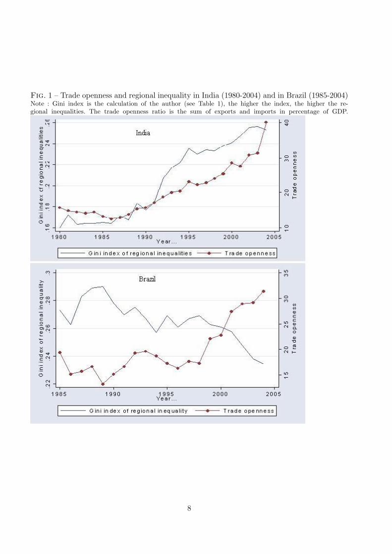
Fig. 1 – Trade openness and regional inequality in India (1980-2004) and in Brazil (1985-2004)Note : Gini index is the calculation of the author (see Table 1), the higher the index, the higher the re-gional inequalities. The trade openness ratio is the sum of exports and imports in percentage of GDP.

8

on regional disparities.

3.1 The determinants of regional inequality

Some of the factors of the level of regional disparities are intrinsic to the country and depend on

countries’ specificities. They are, for instance, the history of the national economic development,

the geographic advantages of some regions and the climate. Fiess and Verner (2003) explain

that the inequality between the northeast and the south of Brazil goes back centuries. The

scope of this paper is not to explain the level of regional inequalities in India and in Brazil

but their evolution over time in the last twenty years. Wei and Wu (2001) argue that studying

inequality in a short time period has one advantage. Any inequality within a country depends

on history, culture, legal system and other national institutions. Over a short time period, these

factors of inequality can be considered as constant and the researcher is more able to isolate

the influence of current phenomena such as trade openness.

New economic geography models predict that trade openness has an impact on regional in-

equality. Then, this prediction is tested empirically by specifying an empirical equation where

regional inequalities are regressed on trade openness. The exclusion of relevant factors of in-

equality potentially correlated with trade openness may result in a biased estimation of the

impact of trade openness variable on inequality. The control for factors that may drive both

trade openness and regional inequality is thus necessary. Other factors of regional inequality can

be omitted from the empirical equation provided they are not correlated with trade openness.

Their effect will be included in the error term and their omission will not introduce substantial

bias in the estimates of coefficients on the trade openness variables.

Foreign direct investment inflows could be a factor of regional inequality in India and in Brazil

and be correlated with their trade liberalization. FDI are concentrated in both countries in

the most developed states. Hansen and Rand (2006) show that FDI convey advantages to host

countries and that they have a positive effect on growth. FDI is also seen as a vehicle for

technological spillover. By promoting the growth of richer states, the concentration of FDI in

richer Indian and Brazilian states probably aggravates the economic gap between rich and poor

states. Thus, inflows of FDI are included as a determinant of regional regionalities and are

expected to exarcerbate them.

Per capita income of the country is also included in the empirical equation as determinant

of regional inequality. Indeed, literature has expressed the idea of a non-linear relationship

between economic development and regional inequalities. Indeed, Williamson (1965) or Lucas

(2000) argue that regional inequalities follow an inverted U-shaped curve depending on the

country’s level of development. Regional inequality should first rise then diminish. At the early

stages of the development process, growth is expected to be spatially unbalanced. According to

Milanovic (2005), the impact of economic development on regional inequality depends on what

drives growth. When growth is fuelled by agricultural growth, growth can foster convergence

and reduce regional inequality. When growth is fuelled by industrial growth and that industries

are subject to agglomerative forces, growth can create regional inequalities. As regards Brazil,

9

Azzoni (2001) finds that fast growth periods are associated with a rise in regional inequalities

in Brazil between 1939 and 1995.

3.2 The empirical equation

To investigate the impact of trade openness on regional inequalities in India and in Brazil, the

time series equation of the following form is specified :

lnGinit = a0 + a1lnOpennesst + a2lnFDIt + a3lnGDPcapitat + ut (2)

The dependent variable is the Ginit index that is the measure of regional inequality for the

year t presented in Table 1. The variable Opennesst is the measure of India’s or Brazil’s trade

openness. This is the sum of exports and imports in percentage of GDP in a given year t, which

is a common measure of trade openness. The trade openness ratio is presented in Figure 1.

The variable FDIt is the net inflows of FDI in percentage of the GDP in India or in Brazil.

Data on FDI are presented in Table 3. The variable GDPcapita is India’s or Brazil’s per capita

GDP in constant 2000 US dollars and is a control variable for the level of development. For all

equations in this paper, t denotes the year t and ln is the log. All data sources are presented

in the Appendix A. Eq. (2) is estimated from 1980 to 2003 for India and from 1985 to 2004 for

Brazil due to availability of the data.

This paper uses the unit root tests, the cointegration techniques and the error-correction models

to test the causal relationship between trade openness and regional disparities. Direct OLS

estimations of Eq.(2) are not appropriate if time series are not stationary. Indeed, there is a

risk of spurious regression when the variables are non-stationary. The econometric methodology

is presented in details in the Appendix B.

4 Empirical results

4.1 Results from the error correction model estimations

First, estimation for Brazil is conducted. Considering Eq. (2), the unit root and time series pro-

perties of all series (lnGinit, lnOpennesst, lnFDIt and lnGDPcapitat) are investigated using

the Augmented Dickey-Fuller and Phillips-Perron unit root tests. For space reason, the test sta-

tistics are not reported in this paper but are available upon request. The unit root test results

indicate that the time series lnGinit, lnOpennesst and lnGDPcapitat are I(1), integrated of

order one. The serie lnFDIt is a TS, that is with a time trend. Having confirmed the existence of

unit root for three time series, the next step involves conducting Engle-Granger two-step coin-

tegration method. The aim is to determine whether the series lnOpenness and lnGDPcapita

are cointegrated with lnGini. Results from the Engle-Granger method show that the variables

lnGinit and lnOpennesst are cointegrated but the variables lnGinit and lnGDPcapitat are not

cointegrated.

10

Since the variables lnGini and lnOpenness are cointegrated in Granger sense, the use of error

correction model (ECM) procedure is appropriate. If two variables are cointegrated, then the

relationship between the two can be expressed as ECM of the following form :

D.lnGinit = a0 + a1residualt−1 + a2D.lnOpennesst + X ′tβ + ut (3)

D. denotes I(1) variables stationarized in first-difference. D. is the differencing operator such

that D.lnGinit is equal to lnGinit - lnGinit−1. The variable residualt−1 is the serie of the

lagged residuals collected from the regression of the variable lnGinit on the explanatory variable

lnOpennesst. X ′t are any exogenous stationnary variables, which are here the GDP per capita

and the inflows of FDI both stationarized. The variable lnFDIt is stationarized by removing

the trend. The ECM of Eq.(3) says that changes in trade openness, in inflows of FDI and in per

capita GDP cause regional inequality to change. The estimation of Eq.(3) is presented in column

2 of Table 2. Column 1 reports the long-run relationships between lnGini and lnOpenness.

In column 2 of Table 2, the trade openness variable D.lnOpennesst yields a negative (-0.11)

and significant coefficient : the opening of the national economy to the foreign market appears

to have reduced regional inequality in Brazil. Milanovic (2005) finds the opposite result for

Brazil since his regression analysis using panel data including India, Brazil, the USA, Indonesia

and China establishs that trade openness results in greater regional inequality. Yet, Milanovic

(2005) and this paper regress the same weighted Gini index of regional inequality. But, while Eq.

(2) is a time series regression for Brazil, Milanovic (2005) uses panel data regressions including

five countries. Besides, the non-stationnarity of the data is not handled, which could explain

the difference in outcomes. Concerning the other factors of regional inequalities, in Milanovic

(2005), the weighted Gini index is regressed on trade openness as well, on GDP per capita, on

interest rate and inflation rate but FDI are not included. In the absence of FDI as an explanatory

variable, trade openness could capture the positive impact of FDI on inequality. In column 2

of Table 2, the coefficient of the lagged residual term included in the ECM is significant and

negative equal to -0.69, which is expected if there exists a cointegration relationship between

the variables lnGini and lnOpenness.

The same econometric methodology is used for India. The series lnGinit, lnOpennesst, lnFDIt

and lnGDPcapitat are found to be integrated of order 1 and the series lnOpenness and lnFDI

are cointegrated with lnGini. If trade openness and the inflows of FDI are cointegrated with

the Gini variable, then the relationship between the three can be expressed as ECM of the

following form :

D.lnGinit = a0+a1residualt−1+a2D.lnOpennesst+a3D.lnFDIt+a4D.lnGDPcapitat+ut (4)

The variable residualt−1 is the serie of the lagged residuals collected from the regression of

the variable lnGinit on the cointegrated variables lnOpennesst and lnFDIt. The estimation

of Eq. (4) is presented in column 4 of Table 2. Column 3 reports the long-run relationships

between the cointegrated lnGini, lnOpenness and lnFDI. The coefficient on the trade openness

11

Tab. 2 – Estimation of the error correction models. Estimation of the impact of trade opennesson regional inequality. Brazil, 1985-2004, and India, 1980-2003.

Dependent variable : Regional inequality (Gini index)Brazil India

lnGinit D.lnGinit lnGinit D.lnGinit(1) (2) (3) (4)

lnOpennesst -.19 .40(.029)∗∗∗ (.041)∗∗∗

lnFDIt .04(.009)∗∗∗

D.lnOpennesst -.11 .40(export + import to GDP) (.064)∗ (.094)∗∗∗

D.lnGDPcapitat -.22 .24(.273) (.310)

lnFDIts or D.lnFDIt* .02 .03(inflows of FDI) (.010)∗ (.010)∗∗∗

residualt−1 -.69 -.71(.215)∗∗∗ (.137)∗∗∗

constant -.76 -.00 -2.74 -.00(.087)∗∗∗ (.007) (.137)∗∗∗ (.015)

observations 20 19 24 23

R2

0.70 0.53 0.96 0.59Note : Robust standard errors in parentheses ; ***, ** and * re-present respectively statistical significance at the 1%, 5% and 10%levels. * The serie is stationarized in first-difference for India andby removing the trend for Brazil.

variable D.lnOpennesst is positive (+ 0.40) and highly significant : the opening of the national

economy to the foreign market appears to have aggravated regional inequality in India. This

result is similar to that found by Milanovic (2005) who finds that greater trade openness results

in more regional inequality in India. However, it is the opposite of that found by Barua and

Chakraborty (2006) who find that trade openness reduced regional inequality in India over

the same period. Their econometric estimation consists in regressing a Theil index of regional

inequality on a trade openness variable using time series. But control variables are not included

in their empirical estimation and the stationarity of the variables is not tested, which could

explain the difference in outcomes.

As said in the introduction, new economic geography models differ concerning their predictions

on the impact of trade on regional inequalities. The empirical results illustrate well this indeci-

siveness since Brazil’s trade openness is found to contribute to a reduction of inequality among

Brazilian states whereas India’s trade openness is found to contribute to a rise of regional in-

equality.

12

The results for the other determinants of regional inequalities are now commented. In the

estimations of the ECM in columns 2 and 4 of Table 2, the coefficients on the FDI variables

are significant and positive, equal to + 0.02 and to +0.03, which indicates that FDI reinforce

regional inequality in India and Brazil. This result was expected. Since the opening of its

economy in the nineties, Brazil has experienced a great increase in inflows of FDI, most of

which has been concentrated in richer regions such as Sao Paulo or Rio Grande do Sul. Indeed

there is clearly a leadership of the southeast region in attracting foreign investment. According

to Bacen (Foreign Capital Census of the Brazilian Central Bank), the southeast concentrated

91% of all assets of firms with foreign control in 1995. FDI probably favor the growth rate of the

host rich states and provides additional advantages to the already well-developed states, thereby

tending to increase regional inequality. FDI were also expected to reinforce inequalities among

Indian states. Indeed, since the liberalization of 1991, India has also experienced a continous

increase in inflows of FDI, most of which has been concentrated in richer states. According to

FDI data of the Indian Ministry of Commerce, the top five states that receive high levels of FDI

between 1991 and 2002 are the richest states (Maharashtra, Tamil Nadu, Karnataka, Gujarat)

and the capital, Dehli. In terms of the destination of FDI flows in 2003, New Dehli (26% of

the total FDI inflows) and Maharashtra (25%) top the list followed by Karnataka (10%), Tamil

Nadu (6%) and Gujarat (4%). FDI probably favor the growth rate of the host rich states,

thereby tending to increase regional inequality. Nunnenkamp and Stracke (2007) who study the

determinants of FDI location and their growth effects in India also find that FDI is likely to

increase India’s regional inequality because FDI are concentrated in already advanced regions

and highly foster their economic growth. Ge (2006) finds a same result for China showing that

FDI reinforce industry agglomeration in China, especially in the coastal Chinese regions that

have the best access to foreign markets.

As regards Brazil and India, in columns 2 and 4 respectively, the coefficients on the variables

D.lnGDPcapita are not significant, which indicates that there is not an instantaneous causality

from economic development to regional inequality in both countries.

Tab. 3 – Net infows of FDI in percentage of countries’ GDP in India and Brazil. Selectedyears over the period 1980-2003.

1980 1983 1985 1987 1990 1993 1995 1997 2000 2003

India 0.04 0.003 0.05 0.08 0.08 0.20 0.60 0.87 0.78 0.76Brazil 0.65 0.40 0.21 0.29 0.69 2.43 5.45 2.01Note : for instance, in 2003, net inflows of FDI account for 2.01% of Brazil’s GDP.Source : WDI, 2004

13

4.2 Robustness checks

4.2.1 Estimating vector error correction models

The aim is to check the robustness of the results on the trade openness variable, which is the

main interest of the paper. A way to test the robustness is to estimate an vector autoregression

(VAR) model or a vector error correction model (VECM) (see Appendix B for more details).

The VAR suggests that the current (time t) observation of regional inequality depends on its

own lags as well as on the lags of each other variable in the equation (trade openness, inflows

of FDI and GDP per capita). All variables are included in the VAR equation after being

stationarized. For both countries, the optimal lag lenght is 2 according to the AIC criterion.

The cointegration between variables is taken into account through including an error term as

in the ECM. The VECM can be expressed of the following form for Brazil :

D.lnGinit = a0 + a1residualt−1 + a2D.lnGinit−1 + a3D.lnGinit−2 + a4D.lnOpennesst−1

+a5D.lnOpennesst−2 + a6lnFDIt−1 + a7lnFDIt−2

+a8D.lnGDPcapitat−1 + a9D.lnGDPcapitat−2 + ut (5)

Estimations of the VECM models are reported in Table 6. Columns 1 and 2 reports the estima-

tions for Brazil and columns 3 and 4 for India. In column 1, Eq. (5) is estimated. The coefficients

on the lagged values of trade openness are significant and negative (-0.16 and -0.15). This means

that lagged values of Brazil’s trade openness are useful in forecasting regional inequality in Bra-

zil : more trade openness means less regional inequality in future, which confirms the results

from the ECM estimation in previous subsection. It is possible to provide a concrete inter-

pretation of this result. The coefficient on the openness variable is equal to -0.16. Assuming

that Gini index in Brazil is equal to 0.26 at year 2000, if Brazil’s trade openness increased

from 20% of GDP to 25% of GDP from year 1999 to year 2000, Gini index should decrease

from 0.26 in 2000 to 0.249 in 2001, which is rather important. An increase in trade openness

reduces the Gini index of regional inequalities. In column 2 of Table 6, the dependent variable

is now Brazil’s trade openness. The lagged values of D.lnGini (regional inequality) and the

error correction term are not significant, which indicates that regional inequality in Brazil do

not Granger-cause Brazil’s trade openness. That is, there is probably one-way causality from

trade openness to regional inequality but not the reverse. Trade openness does not seem to be

endogenous to regional inequality.

Column 3 of Table 6 reports the estimation for India. The regional inequality is the dependent

variable. The coefficients on the lagged values of trade openness are significant and positive

(+ 0.49 and + 0.33), which confirms the results from the ECM regression. Lagged values of

India’s trade openness are useful in forecasting income disparities among Indian states : more

trade openness means more regional disparities in future. Let’s take the coefficient of + 0.49

on the lagged value of trade openness. Assuming Gini index in India is equal to 0.20 at year

1992, if India’s trade openness increased from 20% of GDP to 25% of GDP from year 1991

14

to year 1992, Gini index should increase from 0.20 in 1992 to 0.222 in 1993, which is quite

important. A rise of trade openness increases Gini index of regional inequalities. In column 4

of Table 6, trade openness is now the dependent variable. The lagged values of D.lnGini and

the error correction term are not significant : inequality among Indian states does not seem

to Granger-cause India’s trade openness. There is one-way causality from trade openness to

regional inequality in India but the reverse is not true. In conclusion, the VECM estimations

confirm the results from the ECM estimations. Trade openness reduces regional inequality in

Brazil and aggravates regional inequality in India.

4.2.2 The role of decentralization in regional disparities in India

The preceding analysis assumes that the evolution of regional disparities is influenced by trade

openness, inflows of FDI and national economic development. But another possible determinant

of regional inequalities is fiscal decentralization. Rodriguez-Pose and Gill (2003) show that rising

regional disparities and decentralization have become established trends since the eighties in

China, India, Mexico, Spain, and the US. In the nineties, India favored a greater redistribution of

authority to the sub-national levels. According to the authors, decentralization of expenditures

disadvantages the poorer Indian states whose public investments can not compete with the

richer states. The poorer states became unable to provide infrastructure and services necessary

to attract investments. Kurian (2001), in an official report of the Indian government, also

explains that backward states will not be able to improve their infrastructure and education

facilities because their finances are too deteriorated.

To control for the impact of decentralization on inequalities, lagged values of decentralization

variables are included in the VECM estimation for India in column 5 of Table 6. Data come

from World Bank’s Country Database on Fiscal Decentralization. As regards India, data are

available from 1980 to 1999. The analysis is not conducted for Brazil because of lack of data over

the full period 1985-2003. In column 5, the sub-national share of public expenditures in total

public expenditures, which is a proxy of decentralization (net of expenditures in defense and

interest), is included. This indicator fell from 72.8% in 1980 to 67.7% in 1989. In the nineties,

decentralization increased, up to 73.2% in 1999. This time series is I(1) and is included after

being stationarized. The coefficient on the decentralization variable lagged at two periods is

positive (+1.47) and significant, which indicates that more decentralization of expenditures

means more regional inequalities in India. This result is similar to Rodriguez-Pose and Gill’s

(2003) findings. Besides, trade openness has still a significant impact on regional inequality,

after including the decentalization variable.

4.2.3 The role of composition of trade in regional inequalities

In a new economic geography model, Paluzie (2001) shows that opening to manufacturing

trade increases regional inequalities. She assumes the immobility of the agricultural sector.

Labor force and agricultural inputs are tied to the land and the agricultural population is dis-

persed throughout the national territory, which encourages firms and industries, in a closed

15

economy, to be also dispersed to service the local demand. When the country opens to inter-

national trade, local demand can be replaced by foreign demand and, thus, industrial firms

leave the agricultural regions to agglomerate and benefit from the advantages of concentra-

tion. Besides, an increase in manufacturing exports relatively to agricultural exports will favor

the manufacturing region at the expenses of the agricultural regions. Rodrıguez-Pose and Gill

(2006) provide a similar analysis and argue that changes in trade composition can impact on

regional inequality. When agricultural exports decrease relatively to manufacturing exports,

regional disparities increase. The idea is that agriculture is tied to the land and is (more and

less) equally distributed throuhgout the national territory, whereas manufacturing industry

can be subject to agglomerative forces and be concentrated in one region. Agricultural exports

are favorable to the whole country, while manufacturing exports are directly favorable only to

the industrial center. If manufacturing exports develop at the expense of agricultural exports,

trade favors one region and contributes to a rise of regional inequality. Rodrıguez-Pose and

Gill (2006) find a correlation between the composition of trade and regional inequalities for

eight countries (India, Germany...) but they examine correlation, without controlling for other

factors of regional disparity.

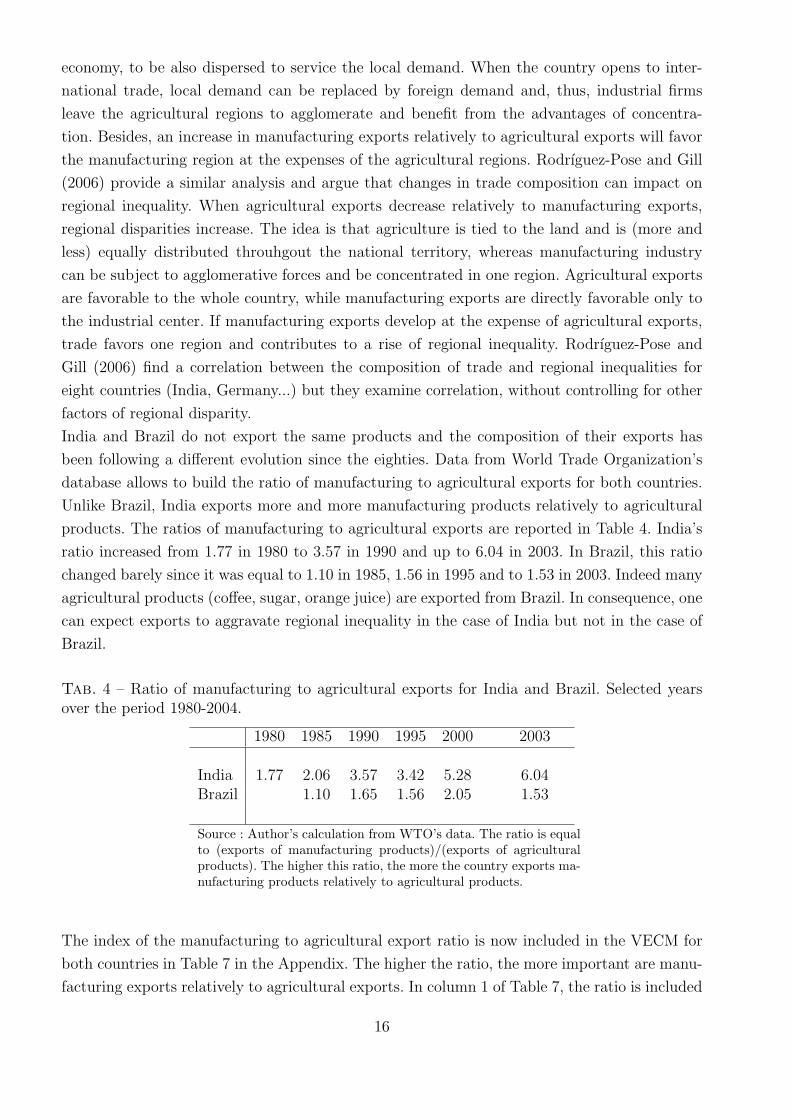
India and Brazil do not export the same products and the composition of their exports has

been following a different evolution since the eighties. Data from World Trade Organization’s

database allows to build the ratio of manufacturing to agricultural exports for both countries.

Unlike Brazil, India exports more and more manufacturing products relatively to agricultural

products. The ratios of manufacturing to agricultural exports are reported in Table 4. India’s

ratio increased from 1.77 in 1980 to 3.57 in 1990 and up to 6.04 in 2003. In Brazil, this ratio

changed barely since it was equal to 1.10 in 1985, 1.56 in 1995 and to 1.53 in 2003. Indeed many

agricultural products (coffee, sugar, orange juice) are exported from Brazil. In consequence, one

can expect exports to aggravate regional inequality in the case of India but not in the case of

Brazil.

Tab. 4 – Ratio of manufacturing to agricultural exports for India and Brazil. Selected yearsover the period 1980-2004.

1980 1985 1990 1995 2000 2003

India 1.77 2.06 3.57 3.42 5.28 6.04Brazil 1.10 1.65 1.56 2.05 1.53

Source : Author’s calculation from WTO’s data. The ratio is equalto (exports of manufacturing products)/(exports of agriculturalproducts). The higher this ratio, the more the country exports ma-nufacturing products relatively to agricultural products.

The index of the manufacturing to agricultural export ratio is now included in the VECM for

both countries in Table 7 in the Appendix. The higher the ratio, the more important are manu-

facturing exports relatively to agricultural exports. In column 1 of Table 7, the ratio is included

16

for India. The ratio is a TS serie and is included stationarized. The coefficient on the lagged

value of the ratio is significant and positive, equal to +0.03 : an increase in manufacturing

exports relatively to agricultural exports increase inequality among Indian states. This result

is confirmed in column 2 when the manufacturing exports in percentage of GDP is included.

Indeed, in India, industries are mainly located in developed states of South India (Mahara-

shtra and Karnataka). In the nineties, manufacturing exports increased greatly relatively to

agricultural exports, thereby favoring the manufacturing area at the expense of the agricul-

tural states. For Brazil, the ratio that is a stationnary serie is included in column 3 of Table

7. The coefficients are negative (equal to -.02) and, as expected, not significant. Last but not

least, if the rich nations accept in the future to open up their markets for agricultural goods, it

could foster the economic growth of the poor agricultural regions in India. But if the European

nations accept such an opening, it could be at the expense of agricultural regions and could

exacerbate regional inequalities within their own territory between agricultural and industrial

regions. It depends how important agriculture is in the economy and how it is distributed over

the national territory.

5 Discussion

Empirical results show that trade openness aggravates inequality among Indian states. A first

explanation is that the increase in manufacturing exports relatively to agricultural exports has

reinforced this inequality. But there may be additionnal mechanisms linking trade openness

and regional inequality in India. Brazil’s trade openness is found to have reduced regional

inequality in Brazil. The regression fails to establish a link between composition of exports and

regional inequality. Links between Brazil’s trade openness and regional disparities have still

to be found. This section discusses some hypotheses on how trade openness might impact on

regional inequalities in both countries.

5.1 Why India’s trade openness increases inequality among states

Crozet and Koenig-Soubeyran (2004) build a theoretical model that predicts that trade libera-

lization can increase regional inequalities depending on the national geography : trade liberali-

zation fosters agglomeration of economic activities in the border region that has the best and

lowest-cost access to foreign markets, thereby creating inequalities between this region and the

remote regions. The purpose is now to determine whether such a scenario occurred in India

atfer the 1991 trade liberalization.

In India, the coastal and southern states have clearly a better access to foreign markets than

the landlocked northern states do. The southern states have always had vast seaports and an

active coastline and, in the past, South India welcame foreign traders and travellers. Nowadays,

industries located in coastal South India can satisfy both the international market and the

internal market. This region has big cities (Mumbay for instance) and is very populated. After

the 1991 trade liberalization, coastal regions may have been advantaged relative to interior

17

regions. Besides, South India has many other intrinsic qualities. The good practice of English,

the good quality of sub-national goverments and of local education (Guha, 2007) made this

region even more attractive for Indian and foreign firms.

But is there any evidence for an agglomeration process in South India after trade liberalization ?

Thanks of the Indian Ministry of Statistics that provides data on state domestic product for each

year, it is possible to calculate that, in 1990, South India (formed by Maharashtra, Karnataka,

Kerala, Tamil Nadu and Andra Pradesh) that represented 32% of Indian population produced

29% of the total Indian output. In 2003, the same states represent 30% of the Indian population

and produce 42% of the total Indian output. Their share in Indian output increased sharply

in the nineties during the liberalization process. Jayanth (2007) reports that Indian firms,

from Reliance Industries and Tatas, to the Mittals and Mahindras, that located in the past

in the northern parts of the country have been moving into New Dehli or into South India

since 1991. The forward group of southern states has come to prominence in manufacturing

and tradable goods. Labor and capital migrate from poor states to rich ones, from northern

states to southern states. FDI also go mainly to most developed states. Okada and Siddharthan

(2007) show that Indian industrial clusters have emerged since 1991 and are now concentrated

in the three clustered regions : the region of the capital New Dehli, in Mumbai-Pune in the

state of Maharashtra, and in Chennai-Bangalore in the states of Karnata and Tamil Nadu. The

proposition here is that Indian coastal states have the best access to foreign markets, due to

the precise geography of the country, and that an agglomeration process has occurred in South

India after trade liberalization, thereby aggravating the inequalities between South India and

North India.

Another channel linking international trade and regional inequality in India could be that of

economic growth. The most recent studies on trade openness and growth such as Calderon,

Loayza and Schmidt-Hebbel (2004) show that the growth effect is almost null for countries

with low levels of per capita income and positive for countries with a good level of development.

According to this point of view, trade openness might be beneficial to more developed Indian

states and detrimental to the other ones, thereby tending to increase regional disparities. In

other words, the richer Indian states in South India and the capital Dehli would benefit from

India’s trade openness because of their good level of development and the lagged regions of

North India would not.

India’s insertion into the global economy is certainly linked to increasing regional disparities.

Currently, the Indian Central government recognises regional inequalities as a threat to national

unity. The problem of rising regional disparities is all the more dangerous since India has a very

high cultural and linguistic heterogeneity. Many Indian states have their own language, culture

and traditions. Besides, 10 Indian states have large populations (between 50 millions and 170

millions). With such large populations, they could become sovereign countries among the largest

ones in the world. There are growing demands for autonomy voiced by southern non-Hindi

states. In a context of federalism and linguistic heterogeneity, large regional disparities can

become a threat to India’s territorial integrity. Political conflicts between forward Indian states

18

and the center have emerged strongly since the Eleventh Finance Commission in 2000. Kurian

(2001) reports that the richest Indian states were clearly against more transfers and against an

increased tax revenue devolution in favor of poorest States. Some southern non-Hindi states no

longer want to subsidise the Hindi-states of the North. In consequence, the richest states demand

for more fiscal autonomy while the populous backward states (Uttar Pradesh for instance) which

cannot be ignored politically by the center demand for more redistributive transfers. In such a

context, regional inequalities could lead in India to more fiscal decentralization (if the Southern

states win) or more fiscal centralization (if the poorest states take the political advantage). In

India, the political disintegration threat could stem primarily from conflict between the centre

and a few rich states that seek greater fiscal autonomy.

5.2 Why Brazil’s trade openness reduces inequalities across Brazi-

lian states

A possible explanation, inspired from Krugman and Livas Elizondo’s (1996) model, would be

that Brazil’s trade openness fostered the dispersion of economic activities from Sao Paulo to the

peripheral regions. Krugman and Livas Elizondo’s (1996) model shows that trade liberalization

may reduce spatial disparities. In the model, repellent forces are congestion costs, pollution,

insecurity and high land costs. These forces encourage firms to move to the peripheral region.

The agglomeration force is the proximity to large consumer markets, to workers and input

suppliers. In autarky, workers follow firms and the centripetal forces are self-reinforcing, ensu-

ring big agglomerations. When the country opens to international trade, consumers and input

suppliers are partly replaced by exports and imports respectively and the attraction of the

economic center is weakening. Then, there is a dispersal of manufacturing firms throughout the

national territory because of the congestion forces.

Brazil opened to international trade in the nineties. Is there any evidence for a dispersal of firms

over the same period ? Regional inequality in Brazil is mainly due to the concentration of the

production in one region, the state of Sao Paulo. This region enjoys a large consumer market,

educated labor and an easy access to foreign markets, which is favorable to concentration.

Industries are concentrated in the Southeast. But there are congestion costs. Sao Paulo is one

of the most expensive places to live in Brazil. The cost of land, traffic congestion, delays,

accidents and environmental problems are important (Jacobi, 2001). There are many local

conflicts with polluting industries. Trade unions are also stronger than those of the periphery.

The periphery region (Amazonia, Northeast and South) provides a smaller domestic market but

has comparative advantages relative to Sao Paulo : it offers low wages, lower production costs

and more space (Tendler, 2000). Moreover, the states of the periphery provide tax exemptions

or subsidies in order to attract firms and the coastal northeast region has a closer access to

European and North American markets thanks to its international ports and airports and the

south of the country has the closest access to Mercosur countries.

Saboia (2001) and Gutberlet (2007) argue that the Brazilian development trend has been

towards industrial decentralization since the beginning of the 1990s. The Annual Survey of

19

Mining and Manufacturing Industry conducted by Instituto Brasileiro de Geografia e Estatıstica

(IBGE) in 2003 also confirms that there has been a change in Brazilian industrial localization

pattern and a reversal of industrial polarization. The region of Sao Paulo has experienced a

downwards trend in terms of industrial production since Sao Paulo’s industrial production

accounts for about 53% of the nation’s industrial output in 1990 and only 40% in 2004. There

has been a rise of new industries and production lines in other regions. Rodrigues (2002)

also confirms the trend towards decentralization of investments away from Sao Paulo and the

extension of production towards the south and the north east of the country. Some firms move

out of the state of Sao Paulo into other states. It seems that indeed an industrial dispersion

occured in Brazil in conjunction with Brazil’s trade liberalization.

6 Conclusion

Regional disparities represent a development challenge in many countries. The persistence of

large regional disparities may pose a threat to a country’s territorial integrity and affect its

political unity. Globalization is frequently cited as a factor of rising disparities across regions

within a country. The investigation of this paper of a causal link between trade openness and

regional inequality is based on two country cases, India and Brazil, and respectively over the

period 1980-2003 and the period 1985-2004.

Empirical evidence from time series analysis shows that Brazil’s trade openness has contributed

to the reduction of income inequality across Brazilian states. An explanation comes from the

composition of trade. Brazil exports many agricultural products relatively to manufacturing

products, which favorized the agricultural regions that are not the richer in Brazil. Another

possible explanation is that Brazil’s trade liberalization has been responsible for the reallo-

cation of some industrial activities to the peripheral regions. The empirical results also show

that the inflows of foreign direct investments reinforce the territorial disparities in Brazil by

being concentrated in richer states. As regards India, the empirical estimations indicate that

greater global integration of India in international trade has gone together with rising regional

inequality. More precisely, this paper shows that a rise of India’s exports, combined with a shift

from exports in agriculture to exports in manufacturing products, could partly explain the rise

of inequality among Indian states. Besides, the opening of the country to the foreign markets

in the nineties may have also generated an agglomeration process in South India that is the

border region with the lowest-cost access to foreign markets. Results also indicate that foreign

direct investment aggravates regional inequality in India by being concentrated in richer Indian

states. This paper shows that the impact of trade openness on regional inequality may depend

on the studied country, on the context in which trade liberalization takes place and on the

composition of trade.

20

References

AGHION P., BURGESS R. and Redding S. (2004) The unequal effects of liberalization : Theory

and evidence from India. Society for Economic Dynamics, Discussion Paper No. 40.

AZZONI C. (2001) Economic growth and regional income inequality in Brazil. The Annals of

Regional Science 35, 133-152.

BARUA A. and CHAKRABORTY P. (2006) Does openness affect inequality ? A case study of

manufacturing sector of India. International Conference, Economic Integration and Economic

Development, Beijing, China.

CALDERON C., LOAYZA N. and SCHMIDT-HEBBEL K. (2004) External conditions and

growth performance. Central Bank of Chile, Discussion Paper No.292.

CROZET M. and KOENIG-SOUBEYRAN P. (2004) Trade liberalization and the internal geo-

graphy of countries. in MAYER T. and MUCCHIELLI J. Mucchielli (Eds) Multinational firms’

location and economic Geography, Edward Elgar, Cheltenham, pp. 91-109.

ENGLE R.F. and GRANGER C.W. (1987) Co-integration and error-correction : Representa-

tion, estimation and testing. Econometrica 55, 251-276.

ENGLE R.F. and YOO B.S. (1987) Forecasting and testing in co-integrated systems. Journal

of Econometrics 35, 143-159.

FIESS N. and VERNER D. (2003) Migration and human capital in Brazil during the 1990s.

World Bank Policy Research, Discussion Paper No. 3093.

GE Y. (2006) Regional inequality, industry agglomeration and foreign trade : the case of China.

World Institute for Development Economics Research, Discussion Paper No.105.

GONZALES RIVAS M. (2007) The effect of trade openness on regional inequality in Mexico.

The Annals of Regional Science 41, 545-561.

GRANGER C.W. (1988) Some recent developments in a concept of causality. Journal of Eco-

nometrics 39, 199-211.

GUHA R. (2007) The better half. Outlook India Magazine, Jul 16 2007.

GUTBERLET J. (2007) The impact of industrial development in Brazil, in Regional Sustainable

Development Review : Brazil, [Ed. Luis Enrique Sanchez], in Encyclopedia of Life Support

Systems (EOLSS).

HORRIDGE M. and DE SOUZA J. (2004) Economic integration, poverty and regional inequa-

lity in Brazil. Center of Policy Studies, Discussion Paper No. 149.

JACOBI P. (2001) The metropolitan region of Sao Paulo. University of Sao Paulo, Discussion

Paper No. 157.

JAYANTH V. (2007) Why the south attracts. The Hindu, Aug 15, 2007.

KRUGMAN P. and LIVAS ELIZONDO R. (1996) Trade policy and the Third World metropolis.

Journal of Development Economics 49, 137-150.

21

KURIAN N.J. (2001) Regional disparities in India. New Delhi, Planning Commission of India.

HANSEN H. and RAND J. (2006) On the causal links between FDI and growth in developing

countries. The World Economy 29, 21–41.

HENDERSON J.V. (1996) Ways to think about urban concentration : neoclassical. Urban

systems versus the new economic geography. International Regional Science Review 19, 31-36.

LUCAS R.E. (2000) Some macroeconomics for the 21st Centrury. Journal of Economic Pers-

pectives 14, 159-168.

MILANOVIC B. (2005) Half a world : regional inequality in five great federations. World Bank

Policy Research, Working Paper No.3699.

NUNNENKAMP P. and STRACKE R. (2007) Foreign direct investment in post-reform India :

likely to work wonders for regional development ? Kiel Institute of World EConomics, Discussion

Paper No. 1375.

OKADA A. and SIDDHARTHAN N.S. (2007) Industrial clusters in India : Evidence from au-

tomobile clusters in Chennai and the national capital region. Institute of developing economies,

Discussion Paper No. 103.

PALUZIE E. (2001) Trade policy and regional inequalities. Papers in Regional Science 80,

67-85.

PALUZIE E., PONS J. and TIRADO D.A. (2004) The geographical concentration of industry

across Spanish regions, 1856-1995. Review of Regional Research 24, 143-160.

RODRIGUEZ-POSE A. and GILL N. (2003) Is there a global link between regional disparities

and devolution ? Research Papers in Environmental and Spatial Analysis No. 79.

RODRIGUEZ-POSE A. and GILL N. (2006) How does trade affect regional inequalities ? World

Development 34, 1201-1222.

SABOIA J. (2001) Industrial decentralization in Brazil in the 1990’s : A dynamic regionally

distinct process. Nova Economia 11, 85-122.

SACHS J., BAJPAI N. and RAMIAH A. (2002) Understanding regional economic growth in

India. Center for International Development, Discussion Paper No.088.

SCHWERT G. W. (1989) Tests for unit roots : a Monte Carlo investigation. Journal of Business

and Economic Statistics 7, 147-59.

WEI S. and WU Y. (2001) Globalization and inequality : Evidence from within China. NBER

Working Paper No. 8611.

WILLIAMSON J. (1965) Regional inequality and the process of national development. Econo-

mic Development and Cultural Change 14, 3-45.

22

Appendix A. Data sources

India

The Republic of India is a federal country consisting of 28 states and seven union territories.

The Gini coefficients are calculated from 19 states that are the largest states comprising 98.2

percent of total Indian population in 2003. To calculate the Gini indicator, one needs GDP per

capita data at current prices (in local currency) and population data for each Indian state and

each year. These data come from the Indian Ministry of Statistics and Programme Implemen-

tation. To my knowledge, GDP per capita data by Indian state are available only from the year

1980, which explains that this paper studies the evolution of regional inequalities only from

this year. The data for the year 2006 are not available. Data for 2005 exist but data are not

reported for a few states, which explains that the studied period ends in 2004. India’s exports

and imports, the net inflows of foreign direct investment (FDI) in India and India’s GDP per

capita come from the World Bank’s World Development Indicator.

Brazil

Brazil is a federal country divided in 27 states. GDP per capita and population data for each

Brazilian state and each year are provided by the Brazilian institute IBGE (Instituto Brasileiro

de Geografia e Estatistica). IBGE provides annual data for the period 1985-2004. Data for

2005 and 2006 are not available. To my knowledge, GDP per capita and population data by

Brazilian state and for each year are available only from 1985 to 2004, which has limited the

studied period by this paper. Brazil’s exports and imports, the net inflows of foreign direct

investment (FDI) in Brazil and Brazil’s GDP per capita come from the World Bank’s WDI.

Appendix B. Econometric methodology

All time series of Eq. (2) have to be tested for a unit root. The Augmented Dickey-Fuller (ADF)

and Phillips-Perron (PP) unit root tests are used. A crucial issue regarding the implementation

of the ADF test is the selection of the number k of lagged first-difference terms in the ADF

estimated equation. ADF tests are estimated from 5 to 0 lags and the number of lags is then

chosen by minimising the Akaike information criterion (AIC). The sequential strategy of the

ADF test is also followed. The ADF test equation is first estimated with a time trend and

a constant. If the time trend is significant, we stop here. If the time trend is not significant,

the ADF equation is estimated with a constant and without a time trend. If the constant is

significant, we stop here. If the constant is not significant, the equation of the ADF test is

estimated without a time trend and without a constant. An alternative unit root test is the

Phillips-Perron test that is also used here to provide robust results on time series’ order of

integration. The implementation of the Philipps-Perron (PP) test also depends on number of

lags. This number is chosen on the basis of the formula reported in Schwert (1989) who suggests

l = T 1/4 where T is the sample size. The paramater is here equal to 2 in view of the used data.

23

After testing the series for stationarity, cointegration must be tested between variables in-

tegrated of same order I(k). A I(1) variable is a non-stationary DS serie that is stationary

in first-difference. The Engle-Granger approach is used here to determine the existence of a

cointegration relationship. It involves the estimation of the cointegration relationship by OLS.

Then, if the residual predicted from this regression is stationary according to an ADF test

and the Engle and Yoo (1987) tables, the variables are said to be cointegrated. If two or more

variables are found to be cointegrated, error correction models will be estimated. If no variables

are cointegrated, Eq.(2) can be estimated with the OLS estimator, after stationarizing the

non-stationary variables.

After estimating the error correction models (ECM), I perform in section 4.2 vector error

correction models (VECM) to provide robustness checks on the results between trade openness

and regional inequality. Granger-causality test is a method for determining whether one time

series is useful in forecasting another. A time series X is said to Granger-cause Y if lagged

values of X provide significant information about future values of Y. A vector autoregression

(VAR) is used to determine whether lagged values of trade openness are useful in forecasting

the evolution of regional inequality in Brazil and in India. The VAR is also useful to test for

the direction of causality and to check that there is one-way causality from trade openness

to regional inequality. A vector error correction model is a VAR with cointegrated variables,

including the error-correction mechanism term. The variables must be stationary in the VAR.

In consequence, the DS I(1) variables are included in first difference and the TS variables

are included stationarized. The optimal lag lenght for autoregressive terms is determined by

minimizing the AIC. Owing to the small number of observations (around 20) for each country,

the VECM are estimated with the lag lenght of 1 and 2 and find that, across all specifications,

the AIC statistics choose the model with a lag lenght of 2.

Appendix C. Empirical estimations and descriptive data

24

Fig. 2 – Regional inequality in India. Per capita income of Indian states in 2001.Source : map of the author. Per capita income is in PPP current dollars.

25

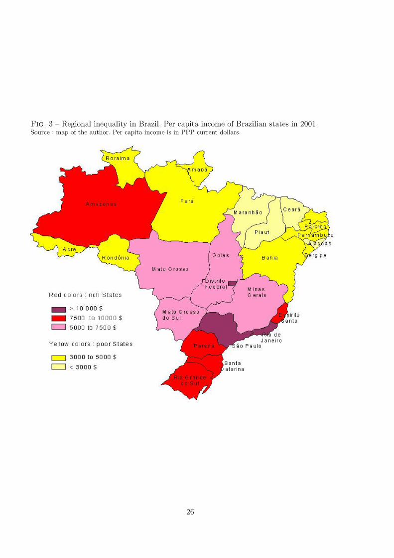
Fig. 3 – Regional inequality in Brazil. Per capita income of Brazilian states in 2001.Source : map of the author. Per capita income is in PPP current dollars.

26

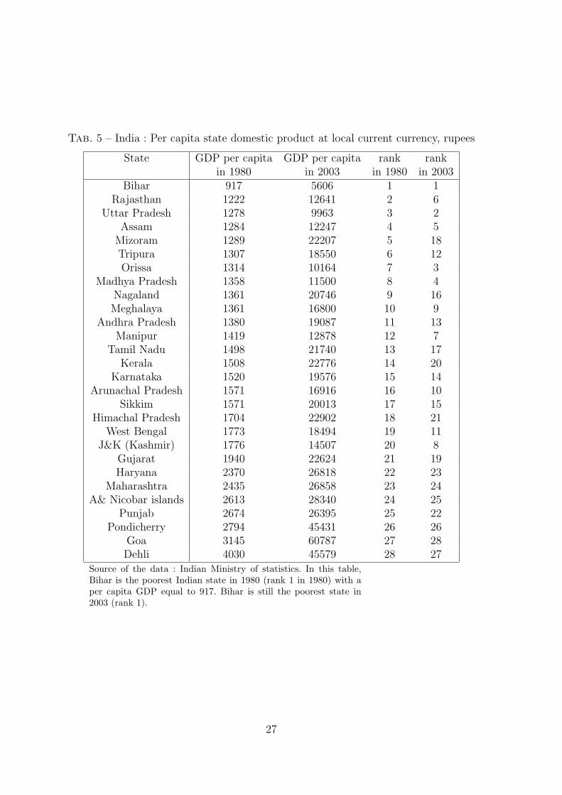
Tab. 5 – India : Per capita state domestic product at local current currency, rupees

State GDP per capita GDP per capita rank rankin 1980 in 2003 in 1980 in 2003

Bihar 917 5606 1 1Rajasthan 1222 12641 2 6

Uttar Pradesh 1278 9963 3 2Assam 1284 12247 4 5

Mizoram 1289 22207 5 18Tripura 1307 18550 6 12Orissa 1314 10164 7 3

Madhya Pradesh 1358 11500 8 4Nagaland 1361 20746 9 16Meghalaya 1361 16800 10 9

Andhra Pradesh 1380 19087 11 13Manipur 1419 12878 12 7

Tamil Nadu 1498 21740 13 17Kerala 1508 22776 14 20

Karnataka 1520 19576 15 14Arunachal Pradesh 1571 16916 16 10

Sikkim 1571 20013 17 15Himachal Pradesh 1704 22902 18 21

West Bengal 1773 18494 19 11J&K (Kashmir) 1776 14507 20 8

Gujarat 1940 22624 21 19Haryana 2370 26818 22 23

Maharashtra 2435 26858 23 24A& Nicobar islands 2613 28340 24 25

Punjab 2674 26395 25 22Pondicherry 2794 45431 26 26

Goa 3145 60787 27 28Dehli 4030 45579 28 27

Source of the data : Indian Ministry of statistics. In this table,Bihar is the poorest Indian state in 1980 (rank 1 in 1980) with aper capita GDP equal to 917. Bihar is still the poorest state in2003 (rank 1).

27

Tab. 6 – Links between regional inequality and trade openness. Estimation of the vector errorcorrection models (VECM). Brazil, period 1985-2004 and India, period 1980-2003.

Brazil IndiaDependent variable :

regional trade regional trade regionalinequality openness inequality openness inequalityD.lnGinit D.lnOpennesst D.lnGinit D.lnOpennesst D.lnGinit

(1) (2) (3) (4) (5)

residualt−1 .34 -.66 .57 -.48 -.18(.287) (.817) (.333)∗ (.300) (.392)

D.lnGinit−1 -.71 .20 -1.07 -.77 -.88(.224)∗∗∗ (1.774) (.528)∗∗ (.723) (.437)∗∗

D.lnGinit−2 -.28 -1.89 -.35 -.54 -.51(.136)∗∗ (1.242) (.265) (.454) (.200)∗∗

D.lnOpennesst−1 -.16 -.05 .49 .51 .33(.046)∗∗∗ (.825) (.269)∗ (.377) (.241)

D.lnOpennesst−2 -.15 .26 .33 .57 .42(.039)∗∗∗ (.634) (.172)∗ (.216)∗∗∗ (.166)∗∗∗

D.lnGDPcapitat−1 .44 -2.37 -1.05 -.48 -.80(.177)∗∗ (1.367)∗ (.700) (.724) (.704)

D.lnGDPcapitat−2 -.51 -.14 -1.30 -1.40 -.92(.171)∗∗∗ (2.043) (.519)∗∗ (.646)∗∗ (.480)∗

lnFDIt−1 .06 .02 .005 -.02 .009(.011)∗∗∗ (.121) (.013) (.027) (.013)

lnFDIt−2 -.04 .11 .01 .01 .02(.010)∗∗∗ (.122) (.009) (.015) (.009)∗

Decentralizationt−1 -.23of expenditures (.635)

Decentralizationt−2 1.47of expenditures (.493)∗∗∗

constant -.006 .04 .09 .08 .08(.003)∗ (.050) (.031)∗∗∗ (.039)∗∗ (.031)∗∗∗

observations 17 17 21 21 18

R2

0.88 0.55 0.57 0.55 0.83Note : Robust standard errors in parentheses ; ***, ** and * re-present respectively statistical significance at the 1%, 5% and 10%levels. For India, FDI is stationarized in first-difference and forBrazil by removing the trend.

28

Tab. 7 – Robustness check. Decomposition of exports as determinant of regional inequality.Estimation of the vector error correction model (VECM) for India, on 1980-2003, and Brazil,on 1985-2004.

Dependent variable : D.lnGinit, regional inequality

India Brazil(1) (2) (3) (4)

residualt−1 .86 .45 .36 .33(.289)∗∗ (.326) (.376) (.392)

D.lnGinit−1 -1.34 -.85 -.73 -.76(.477)∗∗∗ (.355)∗∗ (.309)∗∗ (.318)∗∗

D.lnGinit−2 -.45 -.16 -.26 -.28(.297) (.211) (.149)∗ (.178)

D.lnOpennesst−1 .45 .13 -.14 -.23(.203)∗∗ (.174) (.064)∗∗ (.100)∗∗

D.lnOpennesst−2 .30 .33 -.13 -.18(.174)∗ (.195)∗ (.092) (.069)∗∗∗

lnFDIt−1 .01 -.003 .06 .06(.012) (.009) (.017)∗∗∗ (.011)∗∗∗

lnFDIt−2 .01 .02 -.04 -.04(.009) (.007)∗∗ (.012)∗∗∗ (.010)∗∗∗

D.lnGDPcapitat−1 -1.19 -.87 .49 .43(.550)∗∗ (.482)∗ (.131)∗∗∗ (.150)∗∗∗

D.lnGDPcapitat−2 -1.10 -.87 -.48 -.44(.441)∗∗ (.275)∗∗∗ (.229)∗∗ (.250)∗

(manuf exports/ agricultural exports)t−1 .03 -.02(.017)∗ (.090)

(manuf exports/ agricultural exports)t−2 .005 -.02(.017) (.053)

manuf exports in % of GDPt−1 .25 .06(.094)∗∗∗ (.056)

manuf exports in % of GDPt−2 -.02 .01(.103) (.057)

constant .10 .07 .01 -.006(.028)∗∗∗ (.020)∗∗∗ (.061) (.004)

Observations 21 21 17 17

R2

0.69 0.75 0.88 0.91Note : Robust Standard errors in parentheses ; ***, ** and * re-present respectively statistical significance at the 1%, 5% and 10%levels. For India, FDI is stationarized in first-difference and forBrazil by removing the trend.

29