the impact of transportation costs and trade barriers …

THE IMPACT OF TRANSPORTATION COSTS AND TRADE BARRIERS ON

INTERNATIONAL TRADE FLOWS

by

JASON ALAN QUERY

A DISSERTATION

Presented to the Department of Economicsand the Graduate School of the University of Oregon

in partial fulfillment of the requirementsfor the degree of

Doctor of Philosophy

June 2015

DISSERTATION APPROVAL PAGE

Student: Jason Alan Query

Title: The Impact of Transportation Costs and Trade Barriers on International Trade Flows

This dissertation has been accepted and approved in partial fulfillment of the requirements for theDoctor of Philosophy degree in the Department of Economics by:

Bruce A. Blonigen Co-chairWesley W. Wilson Co-chairAnca D. Cristea Core MemberDaniel Buck Institutional Representative

and

Scott L. Pratt Dean of the Graduate School

Original approval signatures are on file with the University of Oregon Graduate School.

Degree awarded June 2015

ii

c© 2015 Jason Alan Query

iii

DISSERTATION ABSTRACT

Jason Alan Query

Doctor of Philosophy

Department of Economics

June 2015

Title: The Impact of Transportation Costs and Trade Barriers on International Trade Flows

Because trade is seen as welfare improving for society, governments have long employed

their policy-making powers to increase trade levels. In recent years, no strategy has been more

employed by policy makers than free trade agreements. As free trade agreements become more

popular, world tariff levels rapidly approach zero. Given this, policy makers must look to other

methods to encourage trade. I examine how non-tariff trade barriers impact international trade

levels. By better understanding these trade barriers, policy makers will be able to make more

informed decisions.

To better understand non-tariff trade barriers, I begin with well-known impediments to

trade, including the border effect, transportation costs, and the trade creation and trade diversion

effects of regional trade agreements. I then demonstrate and examine heterogeneity in these trade

costs.

In Chapter II I examine the often-studied border effect, the notion that regions trade more

intra-nationally than internationally. I demonstrate that smaller regions are less attractive to

foreign trading partners than their larger counterparts. Fixed costs of crossing an international

border, as well as more effective marketing methods, mean economically larger U.S. states or

Canadian provinces see a smaller border effect. In Chapter III I look at how transportation costs

incurred within the exporting country impact trade levels. Using a unique instrumental variable

strategy, I show that the cost of getting a good to a port is a significant hindrance to trade.

Finally, in Chapter IV I show that the benefits of joining the European Union are heterogeneous

across countries. This means that while the E.U. may be beneficial on average, it may not be

beneficial for individual countries.

iv

CURRICULUM VITAE

NAME OF AUTHOR: Jason Alan Query

GRADUATE AND UNDERGRADUATE SCHOOLS ATTENDED:University of Oregon, Eugene, ORThe University of Texas at Austin, Austin, TXGonzaga University, Spokane, WA

DEGREES AWARDED:Doctor of Philosophy, Economics, 2015, University of OregonMaster of Science, Economics, 2012, University of OregonMaster of Professional Accounting, 2010, The University of Texas at AustinBachelor of Arts, Economics, 2009, Gonzaga UniversityBachelor of Business Administration, 2009, Gonzaga University

AREAS OF SPECIAL INTEREST:International economics, public economics, and applied econometrics

GRANTS, AWARDS AND HONORS:

Graduate Teaching Fellowship, University of Oregon, 2010-Present

Kleinsorge Summer Research Award, University of Oregon, 2013

Econometrics Scholarship,University of Oregon, 2011

v

ACKNOWLEDGEMENTS

I would like to thank Bruce Blonigen for his assistance in creating this dissertation; his

advice, feedback, and financial assistance were all invaluable. I would also like to thank Wesley

Wilson for his guidance, feedback, and unwavering support. Anca Cristea always had time to

discuss my projects and for that I am eternally grateful. I also thank Daniel Buck for his much

needed non-Economist point of view. In addition, Jonathan Thompson and Logan Lee provided

constant and useful feedback. Jordan Kruse is the best proofreader and best friend a person could

possibly want. This dissertation is significantly better thanks to the help of all of these people.

Any remaining mistakes are entirely my own.

In addition, this dissertation benefited from the feedback of a supportive University of

Oregon Department of Economics. Nicholas Sly, the University of Oregon Trade Group, and

the University of Oregon Microeconomic Group all provided feedback on every part of this

dissertation. In addition, Chapter III benefited from seminar presentations at the Western

Economic Association International Annual Meetings and at Colgate University.

vi

For my parents. Thank you for being the best parents a person could ever hope to have.

vii

TABLE OF CONTENTS

Chapter Page

I. INTRODUCTION . . . . . . . . . . . . . . . . . . . . . . . . . . . . . . . . . . . . . 1

II. MARKET SIZE AND HETEROGENEITY OF BORDER EFFECTS . . . . . . . . . 3

Introduction . . . . . . . . . . . . . . . . . . . . . . . . . . . . . . . . . . . . . . 3

Literature Review . . . . . . . . . . . . . . . . . . . . . . . . . . . . . . . . . . . 4

Theoretical Framework . . . . . . . . . . . . . . . . . . . . . . . . . . . . . . . . 8

Data . . . . . . . . . . . . . . . . . . . . . . . . . . . . . . . . . . . . . . . . . . 12

Empirical Evidence of Systematic Heterogeneity in Border Effects . . . . . . . . 13

Market Size and the Border Effect: Empirical Results . . . . . . . . . . . . . . . 19

Robustness Checks . . . . . . . . . . . . . . . . . . . . . . . . . . . . . . . . . . 22

Conclusion . . . . . . . . . . . . . . . . . . . . . . . . . . . . . . . . . . . . . . . 25

III. INTERNAL TRANSPORTATION COSTS AND INTERNATIONAL TRADE . . . . 27

Introduction . . . . . . . . . . . . . . . . . . . . . . . . . . . . . . . . . . . . . . 27


Empirical Methodology . . . . . . . . . . . . . . . . . . . . . . . . . . . . . . . . 30

Data . . . . . . . . . . . . . . . . . . . . . . . . . . . . . . . . . . . . . . . . . . 34

Results . . . . . . . . . . . . . . . . . . . . . . . . . . . . . . . . . . . . . . . . . 36

Conclusion . . . . . . . . . . . . . . . . . . . . . . . . . . . . . . . . . . . . . . . 39

IV. TRADE CREATION AND TRADE DIVERSION IN THE EUROPEAN UNION: DOLARGER COUNTRIES BENEFIT MORE? . . . . . . . . . . . . . . . . . . . . . 40

Introduction . . . . . . . . . . . . . . . . . . . . . . . . . . . . . . . . . . . . . . 40


viii

Chapter Page

Model . . . . . . . . . . . . . . . . . . . . . . . . . . . . . . . . . . . . . . . . . . 43

Data . . . . . . . . . . . . . . . . . . . . . . . . . . . . . . . . . . . . . . . . . . 46

Results . . . . . . . . . . . . . . . . . . . . . . . . . . . . . . . . . . . . . . . . . 47

Conclusion . . . . . . . . . . . . . . . . . . . . . . . . . . . . . . . . . . . . . . . 52

V. CONCLUSION . . . . . . . . . . . . . . . . . . . . . . . . . . . . . . . . . . . . . . . 53

APPENDIX: TABLES AND FIGURES . . . . . . . . . . . . . . . . . . . . . . . . . . . . . . 55

REFERENCES CITED . . . . . . . . . . . . . . . . . . . . . . . . . . . . . . . . . . . . . . . 80

ix

LIST OF FIGURES

Figure Page

1. A Map of Provincial Border Effects . . . . . . . . . . . . . . . . . . . . . . . . . . . . 67

2. A Map of State Border Effects . . . . . . . . . . . . . . . . . . . . . . . . . . . . . . . 67

3. Graph of the Implied Border Effect Over Various Importer Market Sizes . . . . . . . 68

4. Imports and Exports Before and After Joining the EU - Austria and Bulgaria . . . . 69

5. Imports and Exports Before and After Joining the EU - Cyprus and Czech Rep. . . . 70

6. Imports and Exports Before and After Joining the EU - Denmark and Estonia . . . . 71

7. Imports and Exports Before and After Joining the EU - Finland and Greece . . . . . 72

8. Imports and Exports Before and After Joining the EU - Hungary and Ireland . . . . 73

9. Imports and Exports Before and After Joining the EU - Latvia and Lithuania . . . . 74

10. Imports and Exports Before and After Joining the EU - Malta and Poland . . . . . . 75

11. Imports and Exports Before and After Joining the EU - Portugal and Romania . . . 76

12. Imports and Exports Before and After Joining the EU - Slovakia and Slovenia . . . . 77

13. Imports and Exports Before and After Joining the EU - Spain and Sweden . . . . . . 78

14. Imports and Exports Before and After Joining the EU - United Kingdom . . . . . . 79

x

LIST OF TABLES

Table Page

1. States Excluded from Previous Literature . . . . . . . . . . . . . . . . . . . . . . . . 55

2. Border Heterogeneity - OLS - Independent Variable ln(XijYiYj

). . . . . . . . . . . . . 56

3. Robustness Check - OLS - Independent Variable ln(XijYiYj

). . . . . . . . . . . . . . . 57

4. Robustness Checks - OLS - Independent Variable ln(

XijYiYj

). . . . . . . . . . . . . . . . . 58

5. Poisson Estimations - Independent Variable(XijYiYj

). . . . . . . . . . . . . . . . . . . 59

6. Negative Binomial Estimations - Independent Variable(XijYiYj

). . . . . . . . . . . . . 60

7. Summary Statistics for Internal Distance by Product . . . . . . . . . . . . . . . . . . 61

8. Products Included in Sample . . . . . . . . . . . . . . . . . . . . . . . . . . . . . . . . 61

9. Internal Distance Gravity Regressions . . . . . . . . . . . . . . . . . . . . . . . . . . . . 62

10. Internal Distance Gravity Regressions: Standardized Coefficients . . . . . . . . . . . . . . 63

11. Internal Distance Gravity Regressions - Various Years . . . . . . . . . . . . . . . . . 64

12. Trade Creation and Trade Diversion in the E.U. . . . . . . . . . . . . . . . . . . . . . 65

13. Individual Trade Creation and Trade Diversion Effects . . . . . . . . . . . . . . . . . 66

xi

CHAPTER I

INTRODUCTION

Because trade is seen as welfare improving for society, governments have long employed

their policy-making powers to increase trade levels. In recent years, no strategy has been more

employed by policy makers than free trade agreements. As free trade agreements become more

popular, world tariff levels rapidly approach zero. Given this, policy makers must look to other

methods of encouraging trade. I examine how non-tariff trade barriers impact international trade

levels. By better understanding these trade barriers, policy makers will be able to make more

informed decisions.

To better understand non-tariff trade barriers, I begin with well-known impediments to

trade, including the border effect, transportation costs, and the trade creation and trade diversion

effects of regional trade agreements. I then demonstrate and examine heterogeneity in these trade

costs.

Chapter II, titled “Market Size and Heterogeneity of Border Effects in Gravity Models of

Trade,” examines the impact of importer market size on the border effect. The border effect is

the idea that Canadian provinces trade more with other Canadian provinces than they do with

U.S. states after controlling for distance and other relevant variables. Because distance controls

for transportation costs, the border effect should represent fixed costs of crossing the U.S.-Canada

border. When selling to a larger market, the per-unit value of these fixed costs is necessarily

lower which makes a larger market a more attractive export destination. In addition, per-person

marketing costs are likely lower for economically larger regions as large cities make reaching

customers easier. I estimate the impact of importer size on the border effect by estimating the

standard gravity model and include an interaction between the border effect and importer size. I

find that a 10% increase in importer market size leads to a 2.6% increase in international trade

relative to intra-national trade. This result is robust to a variety of specifications, including non-

linear estimation.

Chapter III, titled “Differing Trade Elasticities for Intra- and International Distances:

a Gravity Approach,” focuses on the importance of internal trade costs in exporting items

internationally. The gravity model literature typically proxies for trade costs by included a

1

between-country distance variable. While this serves as a good proxy for trade costs incurred in

shipping a good from one country to another, it does not capture the trade costs incurred before

a good leaves the country. I estimate the effect of these internal trade costs by creating a measure

of internal distance, the distance a good travels before exiting the United States. In addition, I

use two different identification strategies to correct for the potential endogeneity bias created by

firms being able to pick their production location. I find that the internal trade costs are a more

important determinant of trade than external transportation costs.

Chapter IV is titled “Trade Creation and Trade Diversion in the European Union: Do

Larger Countries Benefit More?” and focuses on the border effect of the European Union. I

begin by estimating the average trade creation and trade diversion effects of joining the European

Union. Then, by estimating these effects for each member country, I demonstrate that the benefits

and costs of joining the European Union are heterogeneous across countries. I further explore

potential causes of this heterogeneity. I show that one cause of heterogeneous trade creation

and trade diversion effects is importer and exporter market size. In addition, various natural

country groups such as Scandinavian and Eastern Bloc countries face differing results of joining

the European Union.

Each chapter focuses on a different non-tariff trade barrier, but they ultimately seek to

accomplish the same goal. Lowering tariffs is no longer a practical trade-creating policy tool.

By looking at well known trade costs, and explaining precisely how these trade costs impact

trade levels, I seek to create a better informed policy maker. A complete understanding of the

border effect allows policy makers to focus on lowering the fixed costs of crossing the U.S.-

Canadian border. By knowing that internal transportation costs are a larger hindrance to trade

than between country transportation costs, policy makers should set as their main priority

improving the country’s transportation infrastructure. Through fully understanding trade costs,

this dissertation seeks to allow for better-informed trade policy.

2

CHAPTER II

MARKET SIZE AND HETEROGENEITY OF BORDER EFFECTS

Introduction

The gravity model is one of the most successful empirical models employed in the trade

literature. It does a remarkable job of predicting the direction and volume of trade. One

particularly interesting empirical regularity found with the application of the gravity model is the

border puzzle, which Obstfeld and Rogoff (2001) call one of the six major puzzles of international

economics. Stated simply, controlling for relevant factors, regions are significantly more likely to

trade with other regions within their country than with regions outside the home country.

Since McCallum (1995) found that Canadian provinces have an alarmingly high propensity

to trade with other provinces, as compared to U.S. states, ceteris peribus, trade economists have

set out to explain this “border puzzle.” A seminal work on the subject is Anderson and van

Wincoop (2003), which finds that while the border puzzle still remains, when properly specifying

the model used in the border effect literature the magnitude is much smaller than previously

thought.

In this paper, I contribute to the border effect literature in two key ways. First, I

demonstrate that the border effect is heterogeneous across states and provinces and suggest

one potential cause of this heterogeneity: economically larger regions may have significantly

smaller border effects because the costs associated with crossing the Canada-U.S. border are fixed,

meaning the per-unit impact of these costs are smaller for larger importing markets. My second

major contribution to the border effect literature is that I formalize this “market size” effect both

theoretically and empirically, showing that importer market sizes positively affect international

trade more than intranational trade, even after accounting for multilateral resistance terms. In

addition, I show that a region’s population density is a significant determinant of its border effect.

These empirical results are derived through the use of a unique data set which includes all U.S.

states, something the previous literature frequently fails to consider. I briefly demonstrate that

the exclusion of small states by prior studies leads to a biased estimate of the border effect.

This paper proceeds as follows. In the next section I briefly review the literature on

gravity, border effect, and market size. In section three I discuss the theoretical implications of

3

transportation costs being a function of importer size. In the fourth section, I describe the data

used in the paper. In section five I demonstrate the sampling bias present in previous border

effect papers as well as individually estimate each region’s border effect. I find heterogeneous

border effects and list potential causes for this result. In section six, I test for the presence of the

market size effect. In section seven, I perform a variety of robustness checks. The eighth section

concludes.

Literature Review

Since Tinbergen (1962) developed the gravity model of trade, it has been an empirical

work horse for international trade economists. Though economists have been using the gravity

model since the 1960s, it stood only on its empirical success until Anderson (1979), when it gained

theoretical justification. Now, more than thirty years after Anderson (1979) and more than fifty

years after its introduction, trade economists still use the gravity model to understand the size,

direction, and causes of bilateral trade flows.

One important use of the gravity model has been to explain the importance of trade

costs. In Anderson and van Wincoop (2004), the authors explain that trade costs, especially

non-policy trade costs, continue to be large. Taylor, Robindeaux, and Jackson (2004) argues

that transportation costs at the United States-Canadian border costs the countries $10.3 billion

annually. Disdier and Head (2008) demonstrates that despite market globalization, the distance

effect continues to persist in trade. Hillberry and Hummels (2008) shows that trade costs reduce

the extensive margin of trade, so exporters ship less varieties, with little impact on the per-

unit value of the goods shipped. On the other hand, Chaney (2008) and Helpman, Melitz and

Rubinstein (2008) develop models that show both the intensive and extensive margins changing

with trade costs.

McCallum (1995) employs the gravity model to examine what has become known as

the border puzzle. In the paper, McCallum uses a standard gravity model to examine trade

between Canadian provinces and U.S. states or other provinces, adding only a dummy variable

to indicate if the trade is from one province to another. The author finds that, holding other

relevant variables constant, trade between two Canadian provinces is more than twenty times

larger than trade between that same province and an otherwise identical U.S. state. While it is

4

not particularly unexpected that a province is more inclined to trade with another province, the

magnitude of the border effect was quite surprising and led to considerable follow-up research

attempting to explain the magnitude.

One potential explanation of the border effect is that a border dummy variable is proxying

for tariffs or other trade policies. However, Wolf (2000) shows that state borders matter within

the United States, implying that the border effect must be proxying for more than just U.S. trade

policy. Wolf (2005) finds a similar result in Poland. Hillberry and Hummels (2003) demonstrates

that the Wolf (2000) result is driven by wholesaling, while Millimet and Osang (2007) shows that

controlling for past levels of trade can explain the state home bias. I demonstrate a different

factor in determining the border effect: importer market size.

Likely the most well known follow-up to McCallum (1995) is Anderson and van Wincoop

(2003). In their paper, Anderson and van Wincoop develop a structural specification for

the model McCallum employs, something missing from the original paper. This theoretical

justification makes clear that the McCallum paper suffers from omitted variables bias. Specifically,

the equation should include what Anderson and van Wincoop call a “multilateral resistance”

variable which captures the notion that bilateral trade depends not only on the prices of the two

regions involved, but also the prices of all outside options. Through a demanding econometric

methodology, the authors construct multilateral resistance terms, allowing them to estimate the

border effect consistently and efficiently. While they do find a sizable border effect of roughly

20% to 50%, this number is considerably smaller than the effect discovered in McCallum (1995).

Another key aspect of Anderson and van Wincoop (2003) is the inclusion of state to state trade,

which McCallum had omitted. This allows the authors to examine the border effect going from

Canada to the United States and compare it to the effect of moving from the United States to

Canada. They find that the border effect is much more pronounced for Canadian provinces than

for U.S. states.1

Anderson and van Wincoop (2003) is not without its critics, however. In Santos Silva and

Tenreyro (2006), the authors show that using Poisson Quasi-Maximum Likelihood estimation

techniques yield very different results than one would get using log-linear specifications, as both

McCallum and Anderson and van Wincoop do. I use this as a robustness check to my log-linear

1There also exists a considerable literature examining the border effect using price data, such as Engel andRogers (1996), Parsley and Wei (2000), and Gorodnichenko and Tesar (2009).

5

specifications. By examining the proportions of trade costs paid by buyers and sellers, Anderson

and Yotov (2010) demonstrates that the previous border effect literature suffers from a downward

bias of the border effect variable.

In Balistreri and Hillberry (2007), the authors argue that the Anderson and van Wincoop

assumption of symmetric trade costs is inappropriate. In addition, the authors argue that the

inclusion of U.S. to U.S. trade data is the only driving force behind the Anderson and van

Wincoop result. Using Anderson and van Wincoop’s structural model without state to state

trade alters the McCallum border effect estimate very little, implying that perhaps Anderson

and van Wincoop have not found a “solution” to the border puzzle. In essence, Balistreri and

Hillberry (2007) show that Anderson and van Wincoop’s (2003) estimates suffer from a sampling

bias. Similarly, Matsuo and Ishise (2012) add the missing U.S. states to the Anderson and van

Wincoop sample to document that this exclusion generates sampling bias. My analysis provides

an explanation for the small state sampling bias; I show that this bias can be explained by the

fixed-cost portion of crossing the border resulting in a smaller per-unit impact of the border on

larger markets. An incomplete working paper, Coughlin and Novy (2011), also demonstrates a

size-based omitted variable bias. However, the authors do not explore the connection to marketing

costs as I do in this paper but assume it comes from aggregation bias.

In Redding and Venables (2004), the authors construct a model of trade that yields

a gravity equation that contains exporter and importer fixed effects. Along a similar track,

Feenstra (2002) estimates the border effect gravity equations three different ways: using published

price indexes, using the methods outlined in Anderson and van Wincoop (2003), and including

exporter and importer fixed effects. Feenstra concludes that the fixed effect methodology

produces consistent estimates of the average border effect, while simultaneously being much

easier to implement than the Anderson and van Wincoop (2003) methodology, and thus could

be considered the preferred methodology for estimating border effects. I use this methodology to

account for the multilateral resistance terms in sections six and seven. In “Bonus vetus OLS,”

Baier and Bergstrand (2009) use a Taylor-series expansion to arrive at a consistent method

of estimating gravity models without the econometric rigor of the Anderson and van Wincoop

specification. This methodology has the added benefit of allowing for comparative statics, which

cannot be done in the Feenstra (2002) specification.

6

Recently, Dias (2011b) argues that the trade cost component of the gravity equation should

best be estimated using a polynomial function that would allow distance to enter the gravity

equation in a way not typically employed in the literature. This determination follows from the

author developing a model of trade based on Eaton and Kortum (2002), which Dias modifies to

include FDI and the idea that some trade costs may vary with distance while others may not.

In Dias (2011a), the author argues that an interaction between the border dummy and distance

should be added to the typical gravity equation. In addition, the author argues linear estimation

techniques bias the border effect upward and that non-linear estimation techniques must be

used. Lastly, the author argues that by including the interaction between the border dummy

and distance, the McCallum (1995) border effect disappears, indicating distance matters more

for international trade than it does for intra-national trade. I show that the market-size effect is

present even after controlling for differing distance effects.

My paper is also related to an extensive literature on how both importer and exporter

market sizes impact trade patterns. Exporter market sizes are often linked to trade through a

supply-side story. A seminal paper on the subject is Krugman (1980). In this paper, Krugman

creates a model with transportation costs and economies of scale in production. These

assumptions drive the “market size” effect, which says that locations with a larger market for a

good are more likely to be exporters of that good. Campbell and Hopenhayn (2005) demonstrate

a positive relationship between area population, which they use as a measure of market size, and

average firm size. Combining this with Bernard and Jensen (1999), who demonstrate that larger

firms tend to export, and the resulting implication is that there is a positive relationship between

exporter market size and exporting. However, none of these papers relate any market size effect to

the border effect, as I do in this paper.

There are also papers discussing the impact of importer market size on trade. One such

paper, Eaton, Kortum and Kramarz (2005), shows that the fixed costs of entering a market as

outlined in Melitz (2003) and Chaney (2008) are an important determinant of the relationship

between market size and firm entry. Another paper is Arkolakis (2010). Arkolakis creates a

model using the general framework of Melitz (2003) and Chaney (2008), adding a“marketing

cost.” The cost of reaching a certain number of consumers is assumed to be decreasing in the

market’s population size while reaching the next customer in a given market is increasing in cost.

7

This allows Arkolakis to reconcile trade models with the finding of Eaton, Kortum, and Kramarz

(2011) that the number of exports to a given market is positively associated with the size of the

market. In contrast to these papers, I am taking the further step of linking importer market size

to the magnitude of the border effect.

Theoretical Framework

There exist fixed costs of crossing the border between the United States and Canada.

These can include delays in clearing customs or fees associated with understanding regulatory

requirements for crossing the border. Indeed, in 1993 (the year of my data), with the Canada-

United States Free Trade Agreement well into its life, there likely are very few variable costs

associated with crossing the Canadian-U.S. border. As such, these fixed costs could potentially

explain much of the border effect. In addition, because these costs are fixed, the costs being

spread across more goods implies that the costs have a smaller impact on larger markets. I call

this effect, in the border effect context, the “market size effect.” Thus, the border effect could be

explained in part by the importer market size.

I develop a model that highlights why this market-size effect on the border is important to

capture. I adapt a model by Eaton and Kortum (2002), explicitly making trade costs a function of

importer market size. This allows for very different outcomes when employing comparative statics.

The model outlined in Eaton and Kortum (2002) is well suited as a framework for my empirical

model developed below, as it results in an empirically testable gravity equation, and it does so by

allowing for multiple regions to produce homogeneous, rather than differentiated goods.

The Eaton and Kortum (2002) model is one of Ricardian trade, where firms have access to

differing technologies. There is a continuum of goods k ∈ [0, 1], region i’s efficiency in producing k

is denoted by zi(k), the cost of a bundle of inputs is region - but not good - specific, and is labeled

ci, and there are constant returns to scale. This results in a cost of producing good k in region i

of cizi(k) .

Region i’s efficiency (or technology) at producing good k, zi(k), is assumed to be a random

draw from a region-specific probability distribution Fi(z) = Pr[zi ≤ z]. By the law of large

numbers, Fi(z) is the fraction of goods in region i whose efficiency is less than z. As in Eaton

and Kortum (2002), I assume that the distribution of efficiencies in a region follows a Frechet

8

distribution, so that

Fi(z) = e−Tiz−θ

(2.1)

where Ti > 0 is the location of the distribution and can be thought of as the state of technology

in region i, and θ is the variation in the distribution. The variable θ is assumed the same for

all regions. A larger Ti implies a higher probability of a larger efficiency draw for any good k.

A higher θ implies less variation in the distribution. Thus, according to Eaton and Kortum, Ti

governs a region’s absolute advantage, while θ governs its comparative advantage.

Trade costs follow the typical iceberg assumption. That is, delivering one unit of a good

from exporter region i to importer region j requires producing and shipping dij units of the

good, where dij is referred to as trade costs. A few underlying assumptions about the trade cost

component are that dii = 1 so that there are no internal trade costs, that dij > 1 ∀i 6= j so that

there are positive external trade costs and that the triangle inequality holds so that dij < dimdmj .

To reflect that trade costs may be a function of importer market size, I adapt the Eaton

and Kortum (2002) model to explicitly make the trade cost parameter a function of importer

market size, denoted Yj , but not exporter market size, so that trade costs are equal to dij(Yj).

The effects of this are immediate. While Eaton and Kortum themselves do not assume identical

trade costs (in other words, that dij = dji), many empirical specifications of the gravity equation

do rely on this assumption. However, in this model, except in the highly unlikely case that Yi =

Yj ∀i 6= j, it is extremely unlikely that the assumption of identical trade costs will hold.2 Note

that I am not assuming that the trade costs are solely determined by importer market size, so it

need not be the case that dij = dmj . For simplicity and clarity, I write the trade cost variable as

dij .

Combining the discussion of trade costs, input costs, and efficiency described above, one

arrives at a price of good k in region j that is purchased from region i:

Pij(k) =

(ci

zi(k)

)dij (2.2)

2It is technically possible for the trade costs to be identical, so that dij = dji even if it is not the case thatYi = Yj ∀i 6= j. This can be true if any other relevant variable for determining trade costs between partners vary ina way that exactly offsets the differing size effect. However, while it may be probable for a few trade pairs to havethe same trade costs in either direction, it remains highly unlikely for all trade pairs.

9

The model is one of perfect competition, so the price actually paid in region j for good k can be

written as:

Pj(k) = min {Pij(k); i = 1, ..., N} (2.3)

where N is the total number of regions, including region j. Consumers buy Q(k) amounts of good

k in order to maximize the CES utility function

U =

[∫ 1

0

Q(k)(σ−1)/σ) dk

] σσ−1

(2.4)

subject to the budget constraint that the total spending in region j is equal to Yj , where σ > 0 is

the elasticity of substitution.

Substituting equation 4.2 into equation 2.1 yields the following distribution of prices from

region i to region j:

Gij(p) = Pr[Pij ≤ p] = 1− Fj(cidij/p) (2.5)

Gij(p) = 1− e−[Ti(cidij)−θ]pθ (2.6)

If the lowest price at which region j can purchase a good is from purchasing domestically, they

will do so. Thus, the lowest price in region j will be less than the domestic price p so long as at

least one region, m, satisfies the constraint pmj < p. This implies that the distribution of goods

region j imports, Gj(p) is given by:

Gj(p) = 1−N∏i=1

[1−Gij(p)] (2.7)

Substituting equation 2.6 into equation 2.7 then gives:

Gj(p) = 1− e−Φjpθ

(2.8)

where Φj =∑Ni=1 Ti (cidij)

−θ. As Eaton and Kortum note, Φj , which they call the price

parameter, is an important component of trade analysis because it shows how world technological

levels Ti, world input costs ci, and geographic trade barriers dij impact the prices for any given

region j. Remembering that because dij is a function of importer market size Yj , Φj is also

determined by Yj .

10

Eaton and Kortum (2002) note an important result from this analysis. The probability that

region i is the lowest cost supplier of a good is given by:

πij =Ti (cidij)

−θ

Φj(2.9)

Due to the assumption of a continuum of goods, this also represents the fraction of goods that j

buys from i. Calling Yj region j’s total spending and Xij the amount of spending in region j on

goods from region i, this yields:

Xij

Yj=Ti (cidij)

−θ

Φj=

Ti (cidij)−θ∑N

k=1 Tk (ckdkj)−θ (2.10)

By noting that region i’s total sales, Qi is given by:

Qi =

N∑m=1

Xim = Tic−θi

N∑m=1

d−θimYmΦm

(2.11)

solving for Tic−θi , and substituting these into equation 2.11 gives an expression for the sales from

region i to region j analogous to the typical gravity equation:

Xij =

(dijPj

)−θ∑Nm=1

(dimPm

)−θYm

YjQi (2.12)

Note that exporter sales Qi and importer purchases, Yj , can be thought of as exporter and

importer GDP. As with Anderson and van Wincoop (2003), the exporter GDP enters the equation

with unit elasticity. In addition, the trade between region i and region j depend on world price

levels, not just the price levels of the two regions involved. Recall that dij , the trade costs of

shipping from i to j, are a function of the importer GDP, which is equivalent to Yj . Thus, while

Yj enters by itself as a multiplicative term with unit elasticity, trade between i and j also depends

on Yj through trade costs; thus, Yj does not necessarily have unit elasticity.

This equation is able to highlight the bias generated by ignoring the market size effect when

estimating a gravity equation. To show this, I hold the expression∑Nm=1

(dimPm

)−θYm constant.

Because the gravity model here is not a model over time, this term, which can be thought of as

the multilateral resistance term, will be constant for each given region. This can also be thought

11

of as the small region assumption, such that no state or province is large enough to impact the

price index. Thus, taking the derivative of equation 2.12 with respect to Yj yields:

∂Xij

∂Yj=

(dijPj

)−θQi∑N

m=1

(dimPm

)−θYm

−θ(dijPj

)−1−θQiYj

(∂dij∂Yj

)∑Nm=1

(dimPm

)−θYm

(2.13)

The first component of this derivative is the part typically captured by gravity specifications.

However, the second component is typically ignored by omitting trade cost dij ’s dependence

on importer market size Yj . Because dij is a per unit cost and fixed costs of the market are

likely present, I assume(∂dij∂Yj

)< 0, or that a larger importing market faces lower per-unit

trade costs (through, for example, a more developed and efficient infrastructure); this means

that typical gravity estimation is underestimating the impact of importer market size on trade

flows. In section six, I correct for the omitted variable bias inherent in the previous border effect

specifications.

Data

This paper uses inter-regional trade data for all ten Canadian provinces and fifty U.S.

states in the year 1993. The primary data used for this analysis comes from three primary

sources. These include Statistic Canada’s Input-Output Division, the Canadian International

Merchandise Trade Database, and the U.S. Census Bureau. Interprovincial merchandise trade

data for the year 1993 is provided online by Anderson, and comes from the interprovincial

merchandise trade from Statics Canada’s Input-Output (IO) Division.

Province-to-state and state-to-province trade data comes from the Canadian International

Merchandise Trade Database.3 McCallum (1995) modified these numbers using trade ratios

and the IO trade numbers, while Anderson and van Wincoop (2003) follow Helliwell (1998) in

making the same adjustment at a more detailed industry level. I have opted to not make these

adjustments, with the minor exception of Anderson and van Wincoop’s “rest of U.S.” observation,

which I leave as constructed in their data. I drop all intra-regional trade observations in this

paper. To keep all state trade numbers comparable, I use the unadjusted trade numbers for all

3This database can be located at http://www5.statcan.gc.ca/cimt-cicm/home-accueil?lang=eng

12

states, including those originally in the McCallum and Anderson and van Wincoop specifications.

All trade numbers are converted to 1993 U.S. dollars.

The 1993 Commodity Flow Survey (CFS), conducted by the U.S. Census Bureau, provides

within-state and state-to-state trade numbers for the year 1993. The reported trade numbers

are then scaled down by a factor of 3,025/5,846 for consistency with Anderson and van Wincoop

(2003). This scaling was performed by Anderson and van Wincoop for three reasons. First, while

the Canadian trade data contains only shipments from source to final user, the CFS data contains

all shipments. In addition, goods intended to be exported but first shipped domestically are

included in the CFS data. Lastly, the CFS data does not include agriculture or parts of mining

that are included in the Canadian data. This scaling methodology is not without its detractors.

See, for example, Balistreri and Hillberry (2007).

Of the 3600 trading pairs in the sample, 297 are excluded from the log-linear regressions;

73 pairs are excluded because the value of exports from one partner to the other is zero, so when

the value of trade is logged these become undefined. These pairs are included in the non-linear

estimations presented. The other 224 are excluded because there is not sufficiently reliable data

on trade from the relevant origin to the relevant destination. Of these 297 omitted pairs, 114

have either Alaska or Hawaii as one of the partners and would be omitted from the 48 state

specifications anyway. Other exporting regions that omit more than 10% of their partners are

Kentucky, Louisiana, North Dakota, Oregon, Rhode Island, West Virginia, and Wyoming.

Distances between interprovincial pairs, interstate pairs, and province-to-state pairs were

taken from Anderson, who used kilometer greater circle distances from each regions’ capital. The

gross product of Canadian provinces were taken from Statistics Canada. Gross state products for

U.S. states were taken from the Bureau of Economic Analysis.4

Empirical Evidence of Systematic Heterogeneity in Border Effects

Reasons for Modifying the Anderson and van Wincoop Sample

In McCallum (1995), only thirty states and ten Canadian provinces are included in the

data set. A list of states excluded in McCallum can be found in Table 1 (see Appendix for all

tables). McCallum notes that these thirty states make up 90% of Canada-USA trade in the

4GSP can be located at http://www.bea.gov/newsreleases/regional/gdp state/1998/gsp 0698.htm

13

year he examined. Desiring to remain comparable with McCallum, Anderson and van Wincoop

(2003) also used only thirty states, though they constructed a “rest of U.S.” observation from the

additional twenty states and the District of Columbia. As such, much of the literature on border

effects has been written without incorporating the full set of states in the United States.

This omission of certain states potentially results in sampling bias. McCallum’s sample

includes only those states that border Canada or are the largest, by economic size, in the United

States. Table 1 lists those states omitted from McCallum’s sample. Trade theory (and indeed the

gravity equation itself) says that these states should have systematically higher trade numbers

with Canadian provinces than those excluded from the sample. I begin by examining if adding

these twenty states significantly impacts border effect estimates using a gravity equation that uses

importer and exporter fixed effects to control for multilateral resistance terms.

I estimate the gravity model using the Anderson and van Wincoop sample, which adds

state to state trade to the McCallum sample, using only the 30 states included in the paper and a

“rest of U.S.” composite y. I also estimate the gravity equation using all 48 states.5 To estimate

these equations, I follow Feenstra (2002), who demonstrates that importer and exporter fixed

effects control for multilateral resistance effects. As such, I estimate the following equation:

ln

(Xij

YiYj

)= β4 ln dij + β5δ

ij + αi + αj + εij (2.14)

where δij is a dummy variable equal to unity if the region i is a province and region j is a state,

or vice versa, and αi and αj are exporter and importer fixed effects respectively. Note here that

δij is a dummy variable indicating international trade.

Table 2 reports the results of the Anderson and van Wincoop specifications. The first

column reports the results for equation 2.14 using the original sample of thirty states and ten

provinces. Column 2 reports the specification with all fifty states, and column 3 removes Hawaii

5Alaska and Hawai’i are excluded for peculiarities other than size, as is typical in much of the state tradeliterature.

14

and Alaska from the specification. All variables are statistically significant at the 1% level and the

border effect is negative in all specifications.

It is important to note that Feenstra estimates an average effect of 4.7, while column 1 of

Table 2 indicates an effect of 6.4 (e1.866). This effect is also greater than that of Anderson and

van Wincoop (5.2). This is likely due to the trade data being unadjusted in these specifications

(though adjusted in Anderson and van Wincoop and Feenstra). Comparatively, the 48 state

specification has an average border effect of 7.46 (e2.009). This number is higher than the

thirty state specification; it represent a 16.5% increase in the border effect. This suggests

that by excluding the 18 states I have added to the specification, Anderson and Van Wincoop

underestimated the border effect. However, it should be noted that the 48-state specification does

not result in a magnitude as high as that of the McCallum specification.

It is also important to test if the 48-state specification is statistically significantly different

from the 30-state specification. To do this, I estimated the equation including all variables in

equation 2.14 as well as each of those variables (including the fixed effects) interacted with a

dummy variable equal to unity if the observation was present in the old sample only. Column

4 of Table 2 reports the results of this significant test. Both the distance effect and the border

effect are significantly different from the thirty state specification at the 1% significance level. The

positive sign and large magnitude of the coefficient for the border dummy interacted with the in-

original-sample dummy indicates that the border effect is much more substantial for the 18 added

states than it is for the thirty included states, implying heterogeneous border effects. These results

provide strong evidence that a sampling bias is introduced by excluding the smaller 18 states

resulting in an underestimation of the border effect, thus verifying the results found in Matsuo

and Ishise (2012), among others. For the remainder of this paper I use the 48 state sample.

15

Heterogeneous Border Effects

Before demonstrating the market size effect discussed in the theoretical model, I first

examine whether regions have differing border effects. To estimate individual region border effects,

I estimate the following equation for each state and province6, restricting either i or j to be equal

to the region of interest:

ln

(Xij

YiYj


ij + εij (2.15)

where Xij is the exports from region i to region j, Yi is the gross product of region i, dij is the

distance from region i to region j, and δij is a dummy variable equal to unity if region i is located

in a different country than region j. Thus, to estimate Texas’ border effect, I estimate equation

2.15 for each observation in which Texas is an importer or an exporter.

Note that this is equation 2.14, but without the fixed effects. The fixed effects are excluded

due to concerns about degrees of freedom. For this reason, I do not claim to have precisely

measured each region’s border effect. Instead, I only use these measures to examine patterns

in region-specific border effects. Later, I estimate market size effects on the border effect using

the full sample where I can employ exporter and importer fixed effects to properly control for

multilateral resistance.

Table 3 reports coefficients on the border dummy, the standard errors of these estimates,

and the border effects for each of the 48 U.S. states, where the border effect is calculated as

e|Border Coefficient|. Table 4 reports these same estimates for all ten Canadian provinces. All

estimated border coefficients are negative and all are statistically significant at the 10% level or

greater except for Michigan and Minnesota, which are negative but statistically insignificant.

The first thing to note is that the border effects for the Canadian provinces are significantly

larger in magnitude than those of the United States, with the smallest border effect for a

6I do not estimate individual border effects for Hawaii or Alaska and also excluded these observations in thecalculation of other regions’ border effects.

16

Canadian province being more than double the largest border effect of any U.S. state. This is

consistent with AvW’s finding that the border has a larger impact on the smaller country.

However, even within Canada there is significant variation in the border effects. British

Columbia (BC) has the lowest border effect of any Canadian province with 11.48, meaning BC is

eleven times more likely to trade with a Canadian province than a U.S. state, controlling for the

effects of gross product and distances. Prince Edward Island has the largest border effect of all

Canadian provinces (and indeed, all regions) with an unrealistic 114.01. In Figure 1 (see Appendix

for all figures), I depict the pattern of border effects for Canadian provinces.

There is also considerable heterogeneity in the border effects of the states, with border

effects ranging from 1.29 to 5.88. Michigan has the smallest border effect, though its border is not

statistically significantly different from one. The same is true of Minnesota, with an estimated

border effect of 1.62. It is interesting to note that both of these states border Canada. New

Mexico has the largest border effect of any U.S. state, estimated to be 5.88. In Figure 2, I show

the pattern of border effects for U.S. states.

One pattern of interest is that larger states generally have smaller border effects. For

example, note that Texas and Florida (two of the states with the smallest border effect) are

among the top five gross state products, whereas Montana (with a very high border effect) has the

fourth lowest gross state product of all states. New York and Illinois are in the top five in gross

state product and also have relatively small border effects. On the Canadian side, Prince Edward

Island has a far larger border effect than any other Canadian province. Its gross product is also

only one fourth of the second smallest province by gross product. One potential anomaly to this

explanation, however, is the state of California. Despite the fact that California has more gross

product than any state or province in the sample, the impact of the border on trade with Canada

is significantly high. One potential explanation for this anomaly is that California trades heavily

with Mexico and as such does not rely on Canadian trade as much as other states. Another

17

potential anomaly is North Dakota, which has the lowest gross product of all included states,

but the border has little impact on its trade with Canada.7

There are many potential causes of this size-dependent border effect heterogeneity. One

potential reason that larger regions tend to show smaller border effects is the omitted variable bias

discussed in Anderson and van Wincoop (2003). The larger a region, the smaller the multilateral

resistance term for that region. If multilateral resistance terms are positively correlated with

a border effect, the omission of importer and exporter fixed effects (and thus the multilateral

resistance term) from equation 2.15 would show larger regions having smaller border effects. All

specifications in section six and seven of this paper correct for this bias by including importer and

exporter fixed effects.

Another potential cause of the heterogeneity is that tariffs may impact different regions in

different ways. For example, a large Canadian tariff on corn production is likely to have a larger

effect on Nebraska or Iowa, which produce large amounts of corn, than Florida, which produces

very little corn. While I believe this is an important potential cause of the heterogeneity, my data

do not contain industry-level trade and as such I am unable to test this. I leave this potential

avenue of border effect heterogeneity for future research.

Dias (2011a) argues for an interaction between distance and the border dummy, but given

Figure 2 this cannot be the complete story. The argument is that international transportation is

different from domestic transportation in such a way that distance matters more to international

trade. This would be the case if international shipping is less competitive than intranational

shipping. While most of the low-border effect states do tend to be in New England or the

Midwest, which are close to the Canadian provinces, Texas and Florida have small border effects

despite their distance from Canada; similarly, Montana, which actually borders Canada, is among

the highest border effect states. I include a test of this potential avenue of heterogeneity in my

7It should be noted that of the potential trading partners in the sample, trade from North Dakota to 8 of thepartners are omitted due to zero trade values or insufficient data. Exports from 15 partners to North Dakota areomitted for the same reason. Thus, North Dakota’s puzzling border effect could be caused by omitted observations.

18

econometric specifications, though it should be noted that Dias (2011a) finds no such effect using

OLS.

As mentioned in the theory section, while the multilateral resistance terms are likely

one part of the explanation for border effect heterogeneity, the “market size effect” is also an

important plausible explanation of size-dependent border effect heterogeneity. In the next section,

I disentangle these two effects by including importer and exporter fixed effects to correct for

multilateral resistance terms while also including an interaction between the border effect dummy

and importer market size to help explain the market size effect.

Market Size and the Border Effect: Empirical Results

To examine the issues discussed in the previous section, I run three new gravity

specifications, all of which are built on the baseline regression model given by equation 2.14. I first

add to equation 2.14 an interaction of the dummy variable and the log of distance in an attempt

to replicate Dias (2011a). In another specification, I add an interaction of the border dummy and

the log of gross product of the importing state or province. Lastly, I add both interactions into

one equation. As such, my preferred specification is:

ln

(Xij

YiYj


ij + β3δij × ln dij + β4δ

ij × lnYj + αi + αj + εij (2.16)

The results of these specification are found in Table 5. Column 1 contains the results of

the specification that includes 48 states and no interaction terms and is included for comparison.

In column 2, I report the specification that includes the interaction of distance and the border

dummy. In column 3, I report the specification which includes the interaction of the border

dummy and the log of the importer’s gross product. Lastly, column 4 reports the inclusion of

both interaction terms as to avoid potential omitted variable bias. Note that all results mentioned

19

below are contingent on trade occurring between the two regions. This is caused by the log-

linearization of the model.

In column 3, I test the market-size effect on the border. Column 3 demonstrates that

gross product impacts the measure of the border effect. Significant at the 1% level, the larger

the economy of a trading partner, ceteris paribus, the smaller the effect the border has on trade.

Specifically, a 10% increase in the total size of an importing state or province would result

in a 2.6% increase in international trade beyond the same market size increase’s impact on

intranational trade. The last column acts as a robustness check, demonstrating that this market-

size effect is robust to the inclusion of the distance-border interaction that Dias (2011a) highlights

as being important.8 The market-size interaction term remains significant at the 1% level (the

distance interaction is significant at the 10% level) and the coefficient estimates, while smaller in

both cases, are nearly the same as when only one interaction term is include. Thus, I conclude

that market size has a larger positive effect for cross-border trade than it does for intranational

trade.

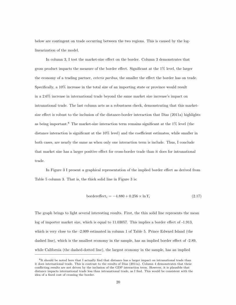
In Figure 3 I present a graphical representation of the implied border effect as derived from

Table 5 column 3. That is, the thick solid line in Figure 3 is:

bordereffecti = −4.880 + 0.256× lnYi (2.17)

The graph brings to light several interesting results. First, the thin solid line represents the mean

log of importer market size, which is equal to 11.03057. This implies a border effect of -1.913,

which is very close to the -2.009 estimated in column 1 of Table 5. Prince Edward Island (the

dashed line), which is the smallest economy in the sample, has an implied border effect of -2.89,

while California (the dashed-dotted line), the largest economy in the sample, has an implied

8It should be noted here that I actually find that distance has a larger impact on intranational trade thanit does international trade. This is contrast to the results of Dias (2011a). Column 4 demonstrates that theseconflicting results are not driven by the inclusion of the GDP interaction term. However, it is plausible thatdistance impacts international trade less than intranational trade, as I find. This would be consistent with theidea of a fixed cost of crossing the border.

20

border effect of only -1.21, significantly smaller than even that of the average border effect.

Perhaps the most important result demonstrated on this graph is the dotted line, the size the

importer would need to be such that there would be no border effect. The log of importer GDP,

in millions, would have to be 18.142. Thus, for a state or province to have no border effect it

would have to have an economy of $75 trillion dollars, or nearly ninety times the 1993 California

economy. Thus, for no plausible region size will the border effect completely disappear.

In the above analysis, I use the interaction of the market size and the border effect to proxy

for a possible effect of fixed costs in crossing the border. However, marketing costs, MCij , are

likely a function of variables beyond just economic size of importer Yj . However, there are other

marketing costs that may impact the border effect. For example, Arkolakis (2010) allows for

the possibility that it is less costly to market to regions with a larger population. To estimate

this potential effect, I include an interaction between the border dummy and importer logged

population density. I use population density, rather than population count, because populations

are not uniformly distributed within regions. One million people concentrated in a region the size

of Rhode Island would likely be much easier to reach with marketing than the same million people

spread across Montana.

The results for these estimations are reported in Table 6. The first column reproduces

the most diverse specification from Table 5. Column two adds the importer population density

interaction, which demonstrates the impact of ease of marketing on the border effect. The first

important result is that importer population density has a statistically significant positive effect.

According to column two, a 10% increase in the population density of an importer will increase

international trade to that region by 1.35% more than intranational trade. This indicates that

population-density based marketing costs are an important determinant of the border effect.

It is also important to note that while the magnitude of the market size effect (the interaction

of the border dummy and the log of importer market size) has changed, the magnitude is not

21

statistically significantly different than that found in column one. As such, both region economic

size and population density of a region are important determinants of that region’s border effect.

Robustness Checks

As mentioned in the previous section, there are many potential explanations for the

observed geographical patterns of individual border effects. In this section, I perform a variety of

robustness checks to assure the reader that the importer market size effect is not simply proxying

for some other cause of heterogeneous border effects. I begin by adding exporter market size into

the specification and by adding a coastal region dummy variable to the specification. I conclude

this section by performing non-linear estimations of the gravity equation.

Exporter Market Size

One potential concern is that importer market size may be highly correlated with any

potential exporter market size effect. The idea that home market demand makes a country more

likely to export a good is a well known concept in the trade literature and is commonly referred

to as the home market effect (see Krugman 1980). Transportation costs make it more costly to

export a good than to sell it locally, so a competitive advantage is given to producers of a good

near the market that demands it. If a larger population results in higher demand for a good,

exporter market size could have a positive impact on trade totals, which may differ when crossing

a border.

To test for this possibility, I run the regression including both an interaction between

importer market size and the border dummy and an interaction between exporter market size

and the border dummy. The results can be found in column 2 of Table 7. The importer market

size interaction is robust to the inclusion of the exporter market size interaction. The importer

market size effect is still significant at the 1% level and positive. In addition, the magnitude is

functionally the same. The exporter market size interaction enters the specification positively and

22

statistically at the 1% level. The regression shows that a 10% increase in exporter market size

will increase trade with international partners by 1.59% more than it would increase intranational

trade. This result is quite interesting. Given the extensive home bias literature, it is no surprise

that exporter market size is an important factor in determining trade. However, the result that

this home bias has a larger impact on international trade is a new one. One potential explanation

of this would be the presence of increasing returns to scale. If the producers of a good face

increasing returns to scale, higher domestic sales potentially makes these producers better able

to overcome any fixed or variable costs of crossing a border.

Coastal States

By noting that Texas and Florida, along with much of the Northeastern United States, in

particular have very low border effects, one may think that having access to a coast, and thus

ocean transportation, may have an impact on the border effect. To allow for this potentiality, I

include in column 3 of Table 7 a dummy variable equal to one if the importing state has an ocean

coast and a dummy variable equal to one if the exporting region is on the coast. Even with the

inclusion of these dummy variables, the market size interaction is still statistically significant and

positive and the magnitude is mostly unchanged.

An importing country having a coastal border has a statistically and economically negative

impact on trade. While this result may seem counterintuitive, it is likely caused by the fact that

this is an examination of trade specifically between the United States and Canada. Coastal access

would have little impact on the transportation costs between states and provinces but would

have a large impact on the transportation costs from European and Asian countries. As such,

these foreign countries may crowd out trade with coastal states and provinces without having

a similar impact on the internal regions. The exporter coastal dummy also enters statistically

significant and negative, but has a much smaller magnitude. Note that the inclusion of these

coastal variables greatly reduces the magnitude of the border effect before the correction for

23

market size. It could be the case that when properly correcting for coastal access, there is a

significantly smaller border effect between the United States and Canada; however, this result

could also be driven by the data-generating process resulting in the misrecording of the origin or

destination of a good. Further research is necessary to see if coastal access can explain much of

the border effect.

In column 4 of Table 7 I include the two coastal dummy variables mentioned above as well

as an interaction between these dummy variables and the border dummy to see if coastal access

impacts intranational trade differently than international trade. The first thing to note is that the

market size effect is still statistically significant and has roughly the same magnitude. Neither of

the coastal interaction terms enter with statistical significance. From this I conclude that coastal

access does not have a differing impact if trade crosses the U.S.-Canada border.

Non-linear Least Squares

Another potential concern is that the importance of importer market size on the border

effect is simply driven by misspecification. Santos Silva and Tenreyro (2006) have observed

that misspecifying the gravity equation as linear biases the coefficient estimates of any gravity

regression. They demonstrate that non-linear techniques, such as Poisson Quasi-Maximum

Likelihood, result in non-biased coefficient estimates. Dias (2011a) demonstrates that log-

linearizing the border effect equation results in border effect estimates that are biased upward. In

this section I estimate the impact of importer market size on the border effect using two different

non-linear estimation techniques.

Since Santos Silva and Tenreyro (2006), Poisson Quasi-Maximum Likelihood (PQML) has

become the preferred estimation method for any gravity equation. In Table 8, I report each of

the results of using PQML to estimate the impact of importer market size on the border effect.

Columns 4 and 5 indicate that the importer market size interaction term loses significance when

I move to a PQML estimation. However, in this specification the standard errors have become

24

significantly large. For example, the standard error of the border dummy in column 5 is more

than ten times larger than the same coefficient’s standard error in column 1. Indeed, the border

effect itself seems to have disappeared! This is likely caused by multicolinearity. Because there

are significantly more intranational trade observations than international trade observations, the

border dummy variable is highly correlated with the market size interaction. As such, I interact

the market size with (1− border effect) in column 6.

The market size effect is statistically significant at the 1% level and moves in the same

direction as the log-linearized specification.9 In addition, the magnitude in the PQML estimation

is more than double that of the log-linear estimation, indicating the log-linear estimation’s

importer market size effect is a conservative estimate. It should also be noted that the sign on

the distance interaction switches signs, and is now consistent with Dias (2011a).

While PQML is the most common estimator used in the recent border effect literature, it

does have its drawbacks. Specifically, it assumes that the mean and standard deviation are equal

to each other. To be sure this is not impacting the results, I also estimate the equations using

a negative binomial estimator. These results are found in Table 9. The coefficient estimates are

nearly identical to those found in the PQML estimations.

Conclusion

The “home bias” or “border effect” puzzle has been a striking empirical oddity since

McCallum (1995). Trade economists have long attempted to explain the magnitude of the border

effect through a variety of econometric and theoretical techniques; perhaps the most successful

example is Anderson and van Wincoop (2003), which explains much of the magnitude of the

border effect as being the result of omitted variables bias.

In this paper, I demonstrate another important omitted variable in the estimation of home

bias: the importer market size’s impact on the border effect. I develop a model based on Eaton

9Because it is now interaction with (1− border effect), the negative sign is now the same as a positive sign inthe log-linear equation.

25

and Kortum (2002) in which trade costs are explicitly a function of importer market size. I

then empirically demonstrate the existence of heterogeneous border effects. From these results,

I provide a mechanism, fixed costs of crossing the border, that potentially explains why larger

markets would experience a smaller border effect.

With this, I empirically estimate how the border effect is impacted by importer market

size. I find that a 10% increase in the market size of an importing country would increase trade

by 2.6% more for cross border trade, thus mitigating the border effect. In addition, importer

population density, proxying for marketing costs, also are important in determining the border

effect. I finish the paper by performing robustness checks to strengthen my result. From these

robustness checks I conclude that importer market size does in fact have a significant impact on

the border effect.

26

CHAPTER III

INTERNAL TRANSPORTATION COSTS AND INTERNATIONAL TRADE

Introduction

International trade economists have long been interested in trade costs. In recent years,

as artificial trade barriers, such as tariffs and quotas, fall to low levels, trade economists have

become more interested in transportation costs as a trade barrier. Because they are difficult to

measure, many trade models proxy for these trade costs with distances between countries. While

the distance between countries, which I call external distance, functions well as a proxy for trade

costs (and has since Tinbergen 1962), it does not give an explicit explanation of trade costs. In

addition, it fails to capture anything not correlated with external distance.

Because of this limitation, there is a significant literature that attempts to explicitly define

trade costs (see for example Anderson and van Wincoop 2004). Transportation costs can be

anything from actual shipping costs to time delays associated with shipping (Hummels and Schaur

2013) to uncertainty associated with maritime piracy (Burlando et al. 2014). The trade cost

literature includes examinations of free trade agreements (Baier and Bergstrand 2007), culture

(Rauch and Trindade 2002), historical and political costs (Head et al. 2010), and the border effect

(McCallum 1995, Anderson and van Wincoop 2003) among many others.

One potentially important trade cost that has received little attention until recently is the

costs incurred in trading before a good leaves the country of origin, which I call internal costs (see

Agnosteva et al. 2014). One probable avenue in which internal costs are important is that a firm

located in a country with high internal costs is at a competitive disadvantage compared to those

firms that can move a good through its location cheaper. While we have many estimates for the

effect of external distance on trade, we know very little about the magnitude of internal distance

as a hindrance to international trade.

27

Little research has been done in this area because internal trade costs and internal distance

can be both extremely difficult to measure and difficult to estimate. No comprehensive data

set exists that allows a researcher to perfectly track the movements of a traded good within

the country of origin. To overcome this obstacle, I combine two data sets, a data set including

commodity-level exports at the U.S. port level and a data set with state-level agricultural

production, to create a unique weighted-average measure of internal distance.

The impact of internal distance on trade is difficult to estimate because it is plausible

that internal distance is endogenous to trade levels. Ceteris paribus, firms which export heavily

will tend to locate production closer to the port of export as a means of reducing internal trade

costs, biasing the estimate of the impact of internal distance. To alleviate this concern, I limit

my sample to agricultural goods, which are constrained in production location by climate and

soil factors. This allows me to use an instrumental variable strategy, where I instrument actual

agricultural production with the Food and Agricultural Organization’s (FAO) Global Agro-

Ecological Zone project’s suitability index. This index essentially ranks the ability of each state

to grow a given agricultural good. The measure is created by the FAO using historical measures of

climate and soil that are independent of U.S. trade patterns.

I find that the internal distance elasticity of trade is statistically significant and large

in magnitude, having a larger impact on trade flows than external distance. I find that, using

conservative estimates, a 10% decrease in the distance a good must travel before leaving the

United States would increase the exports of that good by 16%. These findings have potentially

significant policy implications, particularly with policy makers’ decisions to fund internal

infrastructure.

This paper proceeds as follows. Section two of this paper gives a brief review of the relevant

literature. Section three outlines the empirical specifications and section four details the data used

in this paper. Section five details the results. Section six concludes.

28

Literature Review

This paper contributes to a key literature in international trade which focuses on gravity

models of trade and trade costs. Trade economists have long attempted to explain what exactly

the trade cost component in the gravity model should properly consist of. Authors have examined

the border effect, or the notion that regions are more likely to trade with other regions within

their country as compared to international regions. Examples of these papers include McCallum

(1995), which found the border effect between Canada and the U.S., Anderson and van Wincoop

(2003), which outlined the theoretical justification and an empirical methodology for properly

estimating the border effect, and Query (2014) which shows that the border effect is smaller for

importers with greater GDP. Many papers have examined the potential trade-encouraging effects

of currency and trade unions. Glick and Rose (2002) finds that joining a currency union nearly

doubles trade between the sharing countries. Head et al. (2010) finds that strong colonial ties

can boost trade. Blonigen and Wilson (2008) and Clark et al. (2004) show that the efficiency of

a country’s ports significantly impact trade. Most gravity-based papers examine between-country

trade costs. In this paper, I further attempt to understand how trade costs drive trade flows, but I

am examining the costs a trading firm incurs before a good leaves the country.

Two papers that are directly related to this paper are Agnosteva et al. (2014) and Cosar

and Fajgelbam (2014). A recent paper, Agnosteva et al. (2014) outlines a methodology for

measuring intra-national border barriers and intra-regional trade costs. The paper finds that

intra-regional trade costs are an important consideration in conducting comparative statics.

The paper notes the importance of future research “exploring the connection between intra-

regional and inter-regional trade costs.” Cosar and Fajgelbaum (2014) develops a model which

demonstrates that costly trade leads production to move to areas with easy access to foreign

ports. Reduction in trade costs results in migration to coastal areas. This finding is supported

with data showing that U.S. export-oriented industries are more likely to be located near

international ports. This finding is important to the endogeneity discussion in this paper.

29

Many previous papers examined internal distance, but these papers typically refer to how

far a good bought and sold in the same country travels; they do not consider the effect on related

international trade flows. For a discussion of how various papers measure this type of internal

distance, see Head and Mayer (2002). A few papers do examine internal distance in a similar

fashion to this paper. Blonigen and Wilson (2006) estimates a gravity model which includes

inland transport prices, as well as inland transport distances, though the latter is included in

a market potential variable so no direct internal distance elasticity is estimated. Malchow and

Kanafani (2004) uses the distance a good would have to travel before leaving a port to estimate

the internal distances effect on port choice, though the paper does not look at trade level effects.

While containing no direct measure of distance, Volpe Martincus and Blyde (2013) finds that

firms in Chile which experienced a shock to their transportation network saw a decrease in

the total value of exports. However, because this paper does not contain a measure of internal

distance it does not estimate an internal distance elasticity. Cosar and Demir (2014) uses internal

distance measures to calculate the remoteness of Turkish provinces. The authors demonstrate that

improved road infrastructure results in increased trade levels. Atkin and Donaldson (2014) uses

price gaps to show that intranational trade costs are significantly larger in Ethiopia and Nigeria

than in the United States. For a review of literature related to transportation infrastructure, see

Redding and Turner (2014).

Empirical Methodology

Gravity Model

The model used to econometrically estimate the elasticities associated with internal

and external distance is the gravity model of trade pioneered by Tinbergen (1962) and given

theoretical justification by Anderson (1979). The typical log-linearized specification for trade is

given by:

lnXijk = β1 + β2 lnYi + β3 lnYj + β4Zijk + αi + αj + αk + εijk (3.1)

30

where Xijk is the trade in product k exported by country i to country j, Yi is the GDP of country

i, Zijk is a vector of explanatory variables, αi, αj , and αk are importer, exporter, and product

fixed effects, and εijk is an i.i.d. error term with mean zero and variance one. As outlined in in

Anderson and van Wincoop (2003), this specification should include multilateral resistance terms

for both the importer and exporter, which Feenstra (2002) shows can be accounted for using

importer and exporter fixed effects. Theoretically, β2 and β3 should be equal to one.1 As such, the

gravity equation can be rewritten as:

lnXijk

YiYj= β1 + β4Zijk + αi + αj + αk + εijk (3.2)

Variables often included in Zijk are the distance between i and j, whether i and j share a

common language, whether i and j border each other, and whether i and j share a common

colonial tie. For this paper, I include the distance between country i and j as well as adding a

new variable, the distance good k travels within country i before being exported to country j.

There are a few complications that lead to modifications of equation 3.2 for my data

set. First, because the only exporter in my data set is the United States, Yi and αi cannot be

seperarely identified from the regression’s constant.2 In addition, because the external distance

between the United States and a given country is fixed, I cannot include both a measure of

external distance and the importer fixed effect αj . To allow for a comparison of the magnitude

between internal and external distance elasticities, I will exclude αj from my specifications. This

could lead to a potential bias in my specification, as the importer multilateral resistance term is

not fully accounted for and is potentially correlated with included variables. In addition, I allow

the importer income elasticity of trade to differ from one.

1However, as noted in my result section, when I allow the income elasticity to differ from one, I find an incomeelasticity significantly lower than one.

2The main importance of the exporter fixed effect is to account for country specific effects including thatcountry’s multilateral resistance term, but because there is only one exporter, this fixed effect simply gets subsumedinto the constant without generating any bias.

31

One potential issue with omitting importer fixed effects is that importer-specific factors

that impact trade which are typically subsumed into the importer fixed effect are not accounted

for.3 These omitted variables are unlikely to be correlated with internal distance but may bias

coefficient estimates, especially with regards to external distance. As a result, the regressions I

estimate in this paper will be a variation of the following equation:

lnXjk = β1 + β2 lnYj + β3 lnEXTDISTj + β4 ln INTDISTjk + β5COMLANGj (3.3)

+β6AREAj + β7COMCURRj + β8RTAj + β9CONTIGj + αk + εjk

where Xjk is the value of commodity k exported from the United States to country j, Yj is

the GDP of country j, EXTDISTj is the external distance between the United States and

country j, INTDISTjk is the internal distance of commodity k before being exported to country

j, COMLANGj is a dummy variable indicating if the United States and country j share an

official language, AREAj is the geographic area of country j, COMCURRj is a dummy variable

taking the value of one if the United States and country j share a common currency, RTAj is a

dummy variable indicating if the United States and country j are in a regional trade agreement,

CONTIGj is a dummy variable taking the value of one if the United States and country j have a

contiguous border, and αk is a commodity fixed effect.

Accounting for Production Location Endogeneity

Within-country distance is likely endogenous. It is possible that producers, at least to

some extent, locate their production as close to their customers as is feasible. Thus, producers

of exported commodities likely move closer to the coasts, limiting the within-country distance

traveled (see, for example, Cosar and Fajgelbaum 2014). To accommodate for this potential

endogeneity, I limit my data to agricultural goods. Because of the nature of agricultural goods,

3Any U.S.-specific trade determinants will be in the constant term β1 as the U.S. is the only exporter.

32

production is limited to a specific area where the climate and soil are suited for growing a crop.

As such, agricultural goods are less likely to be subject to this endogeneity concern.

Measuring the distance a good travels within the exporting country before leaving a port

is difficult. One potential problem is that a given good-importer pair will almost certainly not

originate from the same location. Countries that import corn may get corn from both Indiana and

Iowa, for example. In addition, many goods travel through multiple ports for the same importer.

Of the 1,175 country-commodity pairs available in my port trade data set, a mere 421 go through

only one port. The mean number of ports a country-commodity pair goes through is 3.7, and the

most ports a commodity-pair goes through is 48, which is corn to Canada. As a non-Canadian

example, Japan’s imports of soybeans went through 28 different U.S. ports in 2007.

In this paper, I generate a measure of the internal distance of agricultural goods for a given

importer. Due to data limitations, this measure is limited to exports from the United States. I

use state shares of agricultural production, as well as port shares in agricultural exports to a given

importer, to generate a weighted average of all distances a good can travel before leaving the

United States for its final destination. The measure of internal distance for a given commodity

and importer pair, INTDISTjk, is given by:

INTDISTjk =∑s

∑p

Xjkp∑p′ Xjkp′

Pks∑s′ Pks′

dsp (3.4)

where j is the importer, k is the commodity, s is a given state, p is a given port, Xjkp is country

j’s imports of commodity k through port p, Pks is the total production of commodity k in state

s, and dsp is the distance from state s to port p. By constructing a weighted average measure

of internal distance, I place a higher importance on ports frequently used for a given importer-

commodity pair and place little weight on infrequently used ports. In addition, I place a higher

weight on states with larger volumes of production of a given commodity and little weight on

states that grow very little.

33

Table 7 includes summary statistics for INTDISTjk by commodity. Because the United

States is one of the largest countries in the world, by area, it is not surprising to see such large

internal distances for the U.S. Only one good (Tobacco) travels less than 1000 miles, on average,

to a port before being shipped to a country. Tomatoes and Potatoes tend to travel the furthest

within the United States before being exported.

This measure is still subject to endogeneity concerns. Specifically, it could be the case

that crop production locations are determined by the trade demand for these goods. Producers

potentially choose to grow crops as close as possible to the ports their crops will ship through,

even if that location is not the most ideal location for production. To correct for this possible

endogeneity, I create an instrument for INTDISTjk, IVjk, which uses the FAO Global Agro-

Ecological Zone project’s crop suitability index to instrument for actual state agricultural

production. The suitability index uses comprehensive soil and climate data to determine how

suitable the land of a given U.S. state is for growing a given crop. Further details on construction

of this index are in the data section of this paper. The crop suitability index is based only a

state’s climate and soil conditions and thus is independent of the trade process. Thus, I construct

IVjk as follows:

IVjk =∑s

∑p

Xjkp∑p′ Xjkp′

PPks∑s′ PPks′

dsp (3.5)

where all variables previously described are the same and PPks is the crop suitability from the

Global Agro-Ecological Zone project. This measure is used to instrument for INTDISTjk in a

two-stage least squares process.

Data

The data used in this paper come from a variety of sources. The trade data come from

the UN Comtrade database. Comtrade provides trade data for a variety of years and levels of

aggregation. In this paper, I use 4-digit harmonized system 2007 data for the year 2007 and 4-

34

digit harmonized system 1992 data for years 1992, 1997, 2002, and 2007.4 The Comtrade data

does not report which port a good went through, information that is necessary in constructing my

internal distance measure. To handle this, I use the U.S. port to foreign country trade data for the

year 2007 available from the U.S. Census Bureau’s USA Trade Online, which is provided at the

4-digit harmonized system level.

Agricultural data comes from two main sources. Actual agricultural production for the U.S.

comes from the 2007 Agricultural Census. The Agricultural Census has total production by state

for the agricultural products listed in Table 8. A measure of how good a state is at producing

a crop, the crop suitability index, comes from the Food and Agricultural Organization Global

Agro-Ecological Zone (GAEZ). The crop suitability index is a value between zero and one hundred

and is derived from the GAEZ model which estimates the potential crop yield of each state’s

land using average climate data from 1961 to 1990 as well as data on soil resources and terrain-

slope conditions. The index is estimated separately for differing input levels as well as source

of water. In this paper, I use the intermediate input level, rain fed suitability index. The FAO

GAEZ data have previously been used by Costinot and Donaldson (2011), using both actual

and potential production of agricultural goods to measure gains from economic integration. In

addition, it was used in Nunn and Qian (2011) to estimate the potential productivity of potatoes

in Europe, allowing them to estimate the impact of potatoes on population growth.

State-to-port distances are calculated “as the crow flies,” using data on longtitude and

latitude coordinates for each state and port. The location data for each state comes from Google

Maps,5 and is measured at the center of the city with the largest population according to the 2000

U.S. Census. Port location data comes from the U.S. Army Corps of Engineers’ Navigation Data

Center6. Gravity variables come from the CEPII Gravity dataset (see Head et al. 2010).

4For most specifications, I use the HS2007 data as it is the most detailed data available in 2007. Unfortunately,HS2007 data does not exist prior to 2007, so for the year-by-year comparison I use HS1992 even for the 2007estimation.

5Found using http://www.mapcoordinates.net/en.

6The data can be found at http://www.navigationdatacenter.us/ports/ports.asp.

35

Results

Internal Distance Elasticity

To generate estimates of the various distance elasticities, I estimate variations of equation

3.3 using basic OLS and the IV strategy outlined above. Table 9 reports these estimations using

the HS2007 data for the year 2007. Column one is equation 3.3 estimated using the variable

INTDISTjk without any instrumental or control variables, while column two excludes control

variables but uses 2SLS to instrument for INTDISTjk with IVjk. Column three adds the

importer-specific control variables using OLS. Column four uses both importer-specific controls

and the IV strategy.

Both columns one and two have an external distance elasticity near unity in magnitude.

The distance elasticity of trade being close to one makes intuitive sense, but this result is not

often found in empirical estimations. Columns three and four have an external distance elasticity

between -0.445 and -0.465, smaller in magnitude than the results in column one and two. This

indicates that while transportation costs have a significant impact on trade, costs other than

transportation costs such as ease of communication (proxied for by the common language dummy)

also have a significant impact on trade and are highly correlated with between-country distance.

As expected, the contiguity dummy is large in magnitude, though it is only statistically significant

in the IV regression. The regional trade agreement dummy is statistically significant and large in

magnitude in both regressions. The other control variables are not statistically significant in either

specification.

In all specifications, the coefficient on the log of internal distance is negative, ranging from

-1.669 to -2.002, and of a larger magnitude than external distance, which ranges from -0.445 to

-1.068. The last row of Table 9 reports the p-value of the test that the coefficient on internal

distance is equal to the coefficient on external distance. In my most-preferred specification which

is reported in column four, I can reject that the internal distance elasticity is equal to the external

36

distance elasticity at the 5% significance level. A 10% decrease in internal distance would cause a

16-20% increase in trade. This effect is similar to, and potentially larger than, the positive impact

on trade than a 10% decrease in the distance between countries, which would only increase trade

by 4%-11%.

Because EXTDISTj is simply a measure of distance between two points while

INTDISTjk is a weighted average measure of distances, I report the standardized coefficients

for the regressions in Table 10. Using column four as an example, these results say that a

one standard deviation decrease in internal distance will increase trade in a given product

by 0.23 standard deviations; a one standard deviation decrease in external distance will only

increase trade by 0.08 standard deviations. The results here are similar to those of Table 9.

The standardized coefficients on internal distance are always larger in magnitude than the

standardized coefficients on external distance.

This result has potentially important policy implications. Artificial trade barriers, such as

tariffs and quotas, are becoming less relevant given that policies such as free trade agreements

push these barriers toward zero. As such, if policy makers look to reducing non-artificial barriers

as a means to promote trade, these results indicate that internal trade costs are a potentially

fruitful avenue for policy makers to pursue. Not only will improving domestic trade infrastructure

be an effective tool in trade promotion, it also creates important externalities for the country. A

more efficient transportation network in the United States will not only have a strong impact on

the U.S.’s international trade but will also encourage more domestic trade. In addition, domestic

investment is more politically palatable than “international” investment.

Finally, Table 9 shows an income elasticity of trade that is different from the one dictated

by theory. In fact, the income elasticity of trade is around 0.55 in Table 9. This pattern also holds

true in Table 11. While the income elasticity of trade varies year-by-year, going as low as 0.44 in

1992, it hovers around the 0.55 mark for most years and is never close to one.

37

I now use the potential production index to generate IV estimates. The first-stage F-stat

for the instrumental variable is reported in columns 2 and 4. The F-stat is greater than 400, a

strong indication that my instrument is correlated with internal distance. The difference between

columns one and two and the difference between columns three and four are both negligible. The

IV-estimated coefficient is always within one standard deviation of the OLS estimation. The

similarity between the OLS and IV estimates is evidence that farmers are not locating their farms

based on distance to the port of export. Instead, they are potentially choosing production location

based on some other factors, such as soil and climate quality or distance to domestic customers.

Internal Distance Over Time

One natural question that comes from this result is: does this result hold for years besides

2007? To test this, I estimate equation 3.3 using HS1992 data for the years 1992, 1997, 2002, and

2007.7 These results can be found in Table 11. For the years 1992 and 2007, the trade elasticity of

internal distance is about 1.5-1.6%, similar to those found in Table 9. In magnitude, the internal

distance elasticity is statistically significant and greater than the external distance elasticity for all

years, though the degrees to which they are different vary greatly. For 1992, the coefficients on the

two distance measures are different at almost the 90% confidence level while for the years 1997,

2002, and 2007 the coefficients on internal and external distance do not appear to be significantly

different. This indicates that international trade is indeed as responsive, if not more responsive, to

internal distance than external distance.

Table 11 has another interesting result to note. The external distance elasticity was

significantly smaller in 1992 than it is in 2007. In fact, external distance in 1992 has less than

half the impact it does in 2007. In addition, the impact of external distance is monotonically

increasing in time. A plausible explanation for this result could be the tendency of the United

States to move towards exporting those agricultural goods which cost more to ship via boat. This

7Note that this means the 2007 results in Table 9, which uses HS2007 instead of HS1992 data, and Table 11 willdiffer.

38

result is consistent with the finding in Head and Mayer (2000) which shows that external distance

effects have either increased, or remained constant, throughout time.

Conclusion

In this paper, I estimate the elasticity of trade associated with transportation costs that

occur within the exporting county. I accomplish this by generating a measure of the distance

various goods must travel to a port before being exported. I find that trade barriers occuring

within the exporting country have a significant impact on trade flows; the impact of these barriers

are potentially more important than external trade barriers.

In order to properly estimate the internal distance elasticity of trade, I combine multiple

data sets to arrive at a weighted average measure of the distance a good must travel before

leaving the United States. I use state production values and port export data to get an estimate

of internal distance. I then include this estimate in a gravity model of trade as a proxy for

intranational trade costs.

The location of production for a good may be endogenous to trade levels. I accommodate

this potential endogeneity in two key ways. First, I limit my sample to only include agricultural

products. Because agricultural products need the correct soil and climate conditions to grow,

producers have less options when it comes to production location. To further alleviate this, I use

the potential of state land to grow a good as an instrument for actual state production.

I find that internal distance is statistically significant and large in magnitude. In my most

conservative estimate, a 10% reduction in internal distance would result in a 16.49% increase

in international trade. The IV regression coefficients are similar in magnitude to their OLS

counterparts. As such, there is no evidence that agricultural producers are selecting their farm

locations based on their international trading partners.

39

CHAPTER IV

TRADE CREATION AND TRADE DIVERSION IN THE EUROPEAN UNION: DO LARGER

COUNTRIES BENEFIT MORE?

Introduction

Regional trade agreements, including free trade agreements and customs unions, have

increasingly been used to encourage trade between member countries. Perhaps no regional trade

agreement has shaped international trade patterns more than the European Union (E.U.). The

E.U. is the largest economy in the world. In addition it goes further than most regional trade

agreements, having a currency union and allowing for the free movement of labor between many

member nations.

Since the formation of regional trade agreements (RTAs) people have been studying their

effects. Viner (1950) first introduced two major outcomes of joining an RTA: the concepts of trade

creation and trade diversion. Trade creation is the idea that after joining an RTA, two member

countries will trade more with each other. Trade diversion is the idea that member countries will

trade less with non-member countries. Typically, trade is being diverted from more efficient non-

member countries to less efficient member countries because lower trade barriers between member

countries results in a cheaper price despite inefficiencies in production.

In this paper, I contribute to the trade creation and trade diversion literature by

demonstrating that the costs and benefits of joining the E.U. are heterogeneous across member

nations and, as such, previous estimations of the average effect fail to tell the complete story. I

estimate the trade creation and trade diversion effects for each country that joined the European

Union between the years 1962 and 2010 and show that these effects differ from country to country.

Furthermore, I demonstrate a variety of causes for this heterogeneity in trade creation and trade

diversion effects. I provide strong evidence that the economic size of a member nation is a key

40

component of trade creation and trade diversion heterogeneity. Economically larger E.U. members

face smaller trade creation and trade diversion effects; they continue to trade extensively with

non-E.U. members. On the other hand, smaller countries become more dependent on other

E.U. members, importing less from and exporting less to non-E.U. members. Certain country

groups also see heterogeneous effects. On average, countries see a 26% jump in trade with other

E.U. members upon joining the E.U. Similarly, they see a 13.8% decrease in trade with non-E.U.

members. Scandinavian countries, however, see smaller trade creation and trade diversion effects

than the E.U. average. Interestingly, former Eastern Bloc countries see an increase in trade with

E.U. members of 150%, resulting in a trade creation effect that is significantly higher than the

E.U. average. In addition, rather than seeing a decrease in trade with non-E.U. members, Eastern

Bloc countries actually increase their trade with non-E.U. members.

This paper proceeds as follows. In the next section, I briefly review the related trade

creation and trade diversion literature. In section three I outline the model to be estimated.

Section four describes the data used in this paper and section five describes the results. Section

six concludes.

Literature Review

This paper contributes to three key literatures: the regional trade agreement literature, the

related trade creation and trade diversion literature, and the border effect of trade literature. This

paper addresses various aspects of all three literatures while also adding to each.

A sizable literature exists which uses the gravity model of trade to estimate the impact of

regional trade agreements on bilateral trade levels. Head et al. (2010) includes a regional trade

agreement dummy in the gravity equation and finds that trade is greater for two RTA members

than for similar nonmembers. Several papers have included a dummy variable for currency unions

in the gravity model, including Rose (2000) and Nitsch (2002). Both find that a currency union

increases trade, though Nitsch’s effect is half that of Rose’s. Haveman and Hummels (1998) find

41

that RTAs can divert trade away from member countries and they can increase trade for non-

member countries.

A related literature examines the endogenous process of joining an RTA. Baier and

Bergstrand (2004) find that key determinants of joining an RTA include distance between

countries, remoteness of partners from the rest of the world, the economic size of the trading

partners, and the proximity of the trading partners. However, to my knowledge, no paper dealing

with the trade creation or diversion associated with an RTA has examined heterogeneous benefits

of RTAs as I do in this paper. In addition, Baier and Bergstrand (2007) show that the most

appropriate method for handling this endogeneity is doing a panel approach with bilateral and

time fixed effects; I follow their methodology in this paper.

A significant literature exists examining the trade creation and trade diversion effects of

regional trade agreements. Viner (1950) first introduced the concepts of trade creation and trade

diversion. These concepts have been expanded on heavily in the last half century. Panagariya

(2000) is a detailed survey of the theoretical literature dealing with trade creation and trade

diversion. A recent paper estimating these two effects is Magee (2008), which uses fixed effects in

a gravity model to control for the “natural trading partner” hypothesis introduced by Wonnacott

and Lutz (1989) and Krugman (1991). This hypothesis states that partners which previously

had large trade levels are more likely to enter into a regional trade agreement. I deal with this

“natural trading partner” problem by only examining the overall increase in trade during the

period following joining an RTA. Magee (2008) finds that regional trade agreements have a

significant impact on trade both before joining the RTA (“anticipatory effects”) and for several

years after joining. This implies that my estimation results are lower bounds of the trade creation

and trade diversion effects.

Lastly, this paper is related to the literature concerning the border effect, or home bias,

of trade. The idea that, controlling for relevant variables, two regions within a country are

significantly more likely to trade with each other than with international regions was introduced

42

by McCallum (1995) and expanded on by Anderson and van Wincoop (2003) among others.1

One border effect paper of particular relevance is Nitsch (2000). Nitsch finds that the border

effect exists among E.U. members; despite the E.U.’s goal of economic integration, E.U. members

are ten times more likely to trade with themselves than with other E.U. members. Nitsch also

finds that countries with a larger per-capita GDP have smaller border effects. Chen (2004) also

finds border effects among E.U. members and demonstrates that technical barriers to trade and

information costs can explain these border effects. Of note is that both of these papers examine

the country-level border effect rather than a “European Union Border effect.” I treat the E.U.

as one country to estimate the border effect and then further estimate how economic size may

impact the magnitude of the border effect using an idea similar to Query (2014).

Model

This paper uses the gravity model of trade, outlined in Tinbergen (1962), to estimate the

impact of joining the European Union on international trade levels. In addition, I follow the

methodology of Baier and Bergstrand (2007) and include importer-exporter and time fixed effects.

The typical gravity model can then be written as:

lnXijt = β1 + β2 lnGDPit + β3 lnGDPjt + β4 lnGDPPCit + β5 lnGDPPCjt+ (4.1)

β6Zijt + αij + αt + εijt

where Xijt is the trade from exporter i to importer j in year t, GDPi is the gross domestic

product of country i, GDPPCi is the GDP-per-capita of country i, Zijt is a vector of ijt specific

variables, αij are importer-exporter fixed effects, and αt is a time fixed effect.

1A non-exhaustive list includes Wolf (2000), Feenstra (2002), Hillberry and Hummels (2003), and Wolf (2005).

43

Trade Creation and Trade Diversion

To estimate the trade creation and trade diversion effects of joining the E.U., I modify

equation 4.1 to include a set of variables related to a country’s relative status to the E.U. This

results in the following equation:

lnXijt = β1 + β2 lnGDPit + β3 lnGDPjt + β4 lnGDPPCjt + β5 lnGDPPCjt+ (4.2)

β6EUEUijt + β7EUNONEUijt + β8EUROEUROijt + αij + αt + εijt

where EUEUijt is a dummy variable equal to one if both i and j are members of the E.U. in year

t EUNONEU is equal to one if one country is a member of the E.U. in year t and the other is

not, and EUROEUROijt is equal to one of both countries are members of the Eurozone in year

t. The coefficient β6 represents the average percentage trade created between two members by

joining the E.U. and β7 is the average percentage trade decrease, or diversion, from non-E.U.

members which is caused by joining the E.U. As such, theory dictates that β6 should be positive

and β7 should be negative.

Heterogeneity in Trade Creation and Trade Diversion

Equation 4.2 estimates the average trade creation and trade diversion effects of the E.U.

However, there is no reason to suspect that the European Union impacts each member in the

same way. For example, Query (2014) indicates that trade barriers can impact economically-

smaller regions differently than their economically-larger counterparts. The paper argues that

fixed costs of crossing the border result in smaller per-unit costs in larger importing regions.

In addition, the paper argues that easy of marketing to larger regions may be a factor. In this

paper, I demonstrate heterogeneity in the trade creation and trade diversion effects and then

examine multiple causes of this heterogeneity. I expect to see larger E.U. members to see smaller

trade diversion effects. Large E.U. members are likely to be competitive enough to overcome

44

the extra trade barrier created when joining the E.U. On the other hand, smaller E.U. members

may struggle to overcome the E.U. border effect and, as such, will become reliant on large E.U.

members as their main trading partners.

To demonstrate heterogeneity in the trade creation and diversion effects of the European

Union, I estimate the trade creation and trade diversion effects for each country that joined the

E.U. during my sample. Thus, I estimate equation 4.2 for each member country, requiring either i

or j to be the country of interest.

Having demonstrated heterogeneity in trade creation and diversion caused by the E.U., I

explore multiple potential causes of this heterogeneity. Following Query (2014), I explore the idea

that the trade creation and diversion effects of the E.U. may be a function of economic size. Thus,

I estimate the following equation:

lnXijt = β1 + β2 lnGDPit + β3 lnGDPjt + β4 lnGDPPCjt + β5 lnGDPPCjt+ (4.3)

β6EUEUijt + β7EUNONEUijt + β8EUROEUROijt + β9EUEUijt ×GDPi

+β10EUNONEUijt ×GDPi + β11EUEUijt ×GDPj + β12EUNONEUijt ×GDPj+

αij + αt + εijt

Query (2014) suggests that β10 and β12 would be negative if E.U. member countries face the

“border effect” in the same way as U.S. states and Canadian provinces, though this need not be

true. Query (2014) offers no suggestion on the the sign of either β9 or β11.

In addition, I explore the possibility that natural country groups may experience trade

creation and trade diversion differently. I first explore the idea that Eastern Bloc countries

experience trade creation and trade diversion in a manner different than that of the rest of the

E.U. Strong influence from the Soviet Union meant this countries emerged from communism to

embrace capitalist markets during my sample. As such, they are likely to experience economic

shocks differently than other E.U. members. Next, I examine whether Scandinavian and non-

45

Scandinavian states see differing effects of joining the E.U. I suspect these countries may be

different than other E.U. members because of the seeming opposition to the E.U. in Scandinavia.

Norway has not joined the E.U. and neither Sweden or Denmark have joined the Eurozone. The

equation used for these estimations is equation 4.2 but requiring that either i or j be a member of

the relevant group of countries.

Data

The trade data used in this paper comes from the UN Comtrade database. Comtrade

contains imports and exports between partners for many years and varying degrees of dis-

aggregation. For this paper, I use the Comtrade data at the SITC Rev.1 level. I then aggregate

this data to arrive at total importer-exporter trade. This allows me to create a panel from 1962 to

2010. Trade values are adjusted to constant-value using the Consumer Price Index with 1982-1984

as the base year. The CPI comes from FRED.

Unfortunately, this dataset reports Belgium and Luxembourg as one country from 1962

to 1998 and as separate countries from 1999 on. I leave Luxembourg and Belgium as separate

observations from 1999 on to allow for the possibility that smaller countries like Luxembourg face

larger border effects. In addition, I drop East Germany from my specification and treat pre-1991

West Germany as the same country as post-1991 Germany.2

Dates for when each country joined the European Union and the Eurozone were retrieved

from the European Union’s official website. Purchasing-power parity adjusted gross domestic

product and country population come from the Penn World Table and cover the entire panel from

1962 to 2010.

My observations are at the importer-exporter-year level. The countries that join the E.U.

during my sample, and thus are the source of variation in my specifications, are Austria, Bulgaria,

Cyprus, the Czech Republic, Denmark, Estonia, Finland, Greece, Hungary, Ireland, Latvia,

2This details are mentioned for clarity but do not have a significant impact on the empirics present in thispaper.

46

Lithuania, Malta, Poland, Portugal, Romania, Slovakia, Slovenia, Spain, Sweden, and the United

Kingdom. For each of these countries, I have created regression discontinuity graphs on total

trade before and after joining the European Union. That is, I regressed the following equation on

two different time periods for each country that joins the E.U. in my sample, all years before a

country joined the European Union and all years after:

Xit = α+ βt+ εit (4.4)

These graphs can be found in Figures 4 through 14.

Results

This section reports the results of the regressions mentioned in the Empirical Model

section. I begin by estimating the trade creation and trade diversion effects of being a European

Union member. I then individually estimate the trade creation and trade diversion effect

individually for each member state to demonstrate heterogeneous effects. Finally, I investigate

potential causes for this heterogeneity.

Trade Creation and Trade Diversion

Column 1 of Table 12 reports the estimation of equation 4.2. The results are as expected.

A positive coefficient on the E.U. to E.U. trade dummy indicates E.U. member states trade more

with each other than two comparable non-E.U. member countries. This is the trade creation

effect of the E.U. Similarly, a negative coefficient on the E.U./non-E.U. trade dummy means that

E.U. member states tend to trade less with non-E.U. members than two comparable non-E.U.

members. This is the trade diversion effect.

The trade creation coefficient is positive and statistically significant at the 99% confidence

level and the magnitude is economically significant. E.U. to E.U. trade is 26% larger than non-

47

E.U. to non-E.U. trade.3 It is worth noting that this effect is significantly smaller than the border

effect between the U.S. and Canada, which is closer to 300%.4 However, the border effect within

the E.U. may still be as large as that seen in the U.S.-Canada border effect literature. The trade

diversion coefficient is negative and statistically significant at the 99% confidence level. E.U.

member states trade 13.8% less with non-E.U. members than you would see from two comparable

non-E.U. members.5 This effect is economically significant but smaller than the trade creation

effect.

Another result worth noting from column 1 of Table 12 is that the coefficient on the Euro

to Euro trade dummy is not statistically significant. This is evidence that, after controlling for

time and importer-exporter fixed effect, being in the Eurozone does not have trade creation effects

above and beyond that which a member state could expect from being in the European Union.

Individual Trade Creation and Trade Diversion Effects

Column 1 of Table 12 reports the average trade creation and trade diversion effects, but

there is no reason to assume the impact the E.U. has on member nations is uniform. In Table

13 I report the individually estimated trade creation and trade diversion effects as well as their

standard errors. Column 1 of Table 13 reports the coefficient on E.U. to E.U. trade for each

individual country and column 2 reports the standard error for that estimate. Column 3 reports

the individually estimated E.U. to non-E.U. coefficient and column 4 reports that coefficient’s

standard error.

Table 13 shows considerable heterogeneity in the effects of joining the European Union.

Interestingly, only Hungary and Romania have coefficients with the same sign as the average.

Every other country has either a positive coefficient on both variables of interest or a negative

3e0.234 − 1

4See Anderson and van Wincoop (2003) and Feenstra (2002) for estimates of U.S-Canada border effect size.

5e−.149 − 1

48

coefficient on both variables. That is, while on average there is a positive cofficient for E.U.

to E.U. trade and a negative coefficient for E.U. to non-E.U. trade, for most individual E.U.

members either trade with both E.U. countries and non-E.U. countries rose or trade with both

E.U. and non-E.U. countries fell. Countries which saw trade with both E.U. and non-E.U.

countries rise include Bulgaria, Denmark, Estonia, Latvia, Malta, Poland, Slovakia and Slovenia.

Cyprus, Ireland, and the United Kingdom have positive coefficients on both the E.U. to E.U.

and E.U. to non-E.U. coefficients; however, the E.U. to non-E.U. coefficient is not statistically

significant. Neither coefficient is statistically significant for the Czech Republic and Finland.

Several countries see trade decrease both with E.U. countries and non-E.U. countries

on average. For Greece, Lithuania, and Spain, both coefficients are negative and statistically

significant. This implies that for these countries joining the European Union unequivocally

decreased trade. Austria, Portugal, and Sweden have negative and statistically significant

coefficients on E.U. to non-E.U. trade; their E.U. to E.U. coefficient is negative but not

statistically significant. They appear to see trade diversion from non-E.U. members while failing

to see the trade creation effect of the E.U.

A few interesting patterns emerge from this analysis. Both countries that saw the same

coefficients as the average members are from the Eastern Bloc. In addition, it is worth noting

that five of the nine Eastern Bloc countries are included in this group. In fact, the only Eastern

Bloc country that has a negative and statistically significant coefficient on E.U. to E.U. trade is

Lithuania. The European Union seems to have been a significant boost to trade for the Eastern

Bloc. In addition, the two Scandinavian countries that are E.U. members are Denmark and

Sweden. Denmark saw trade rise with both E.U. and non-E.U. members after joining the E.U.

Sweden, however, saw the negative trade diversion effect with no corresponding trade creation

effect. Despite both being Scandinavian countries, they see vastly differing effects of the European

Union. I explore heterogeneity among nation groups later in this paper.

49

Market Size

Given the established heterogeneity in the effect of joining the E.U., I now turn to various

explanations of this heterogeneity. I first examine the “market size effect” documented in Query

(2014). Column 2 of table 12 reports the results for the estimation of equation 4.3. The negative

coefficient on the interaction of importer GDP and the E.U. to E.U. trade dummy indicates that

larger E.U. members see a smaller increase in imports from other E.U. countries. One explanation

for this is that larger countries face a smaller barrier to trade with non-E.U. countries and as

such divert less trade from non-E.U. to E.U. members. The negative coefficient on the interaction

between exporter GDP and the E.U. to E.U. dummy says that larger E.U. members also divert

a smaller fraction of their exports to E.U. members. These two results imply that smaller E.U.

members become reliant on larger E.U. members as they both import and export more heavily

from E.U. members than their larger counterparts, while the larger E.U. members continue to

trade heavily with outside countries.

Another interesting result reported in column 2 of table 12 is the negative coefficient on the

interaction of importer GDP and the E.U. to non E.U. dummy. This goes against the results of

Query (2014) and says that smaller E.U. members see a smaller decrease in non-E.U. trade than

their larger counterparts. A potential explanation for this is that, all else equal, simply joining

the European Union makes a country a more attractive trading partner. This could be because of

implied financial stability, confidence in the reliability of courts and laws, or the ease of extending

trading networks from one E.U. country to another. This result alleviates some of the reliance on

larger E.U. countries for imports as mentioned above. Exporter GDP does not appear to have an

effect on the diversion of exports from non-E.U. to E.U. countries.

Heterogeneous Effects for Differing Nation Groups

Another potential source of heterogeneity is that joining the E.U. impacts groups of nations

differently. Column 3 of Table 12 reports the results for only the Eastern Bloc countries, all of

50

which are members of the European Union.6 Note that the coefficient on E.U. to E.U. trade is

statistically significant at the 99% confidence level and is of a magnitude larger than the average

E.U. to E.U. effect. Eastern Bloc countries see an increase in trade with other E.U. members of

more than 150%.7 This is both statstically and economically significantly different than the 26%

average effect. Not only is the trade creation effect for Eastern Bloc countries higher, but the

coefficient on E.U. to non-E.U. trade is positive and statistically significant. Rather than diverting

trade from non-E.U. countries, the Eastern Bloc countries actually increased trade with non-E.U.

countries after joining the E.U.

These results suggests that the Eastern Bloc countries unequivocally benefit from

joining the E.U. One potential explanation for this result is that, as mentioned previously, E.U.

membership itself acts as a signal of consistent and predictable economic and monetary stability.

Another potential explanation is that Eastern European countries function as export platforms

for the European Union, with significant FDI taking place in these countries due to their E.U.

membership and low wages.

Finally it is important to note that while on average the adoption of Euro has no effect

on trade, for the Eastern Block countries which adopted the Euro the Euro has a positive,

statistically significant, and economically significant impact on trade. The Eastern Bloc countries

trade 42% more with other Eurozone members than with non-Eurozone E.U. countries.8

Column 4 of Table 12 shows the impact of the European Union on Scandinavian countries.9

Unlike the Eastern Bloc, which had all members join the E.U., not all Scandinavian countries

are E.U. members. Norway is not an E.U. member and does not participate in the customs

union, though they do participate in the European Economic Area. No Scandinavian country

6These countries are Bulgaria, the Czech Republic, Estonia, Hungary, Latvia, Lithuania, Poland, Romania, andSlovakia.

7This number is equal to 1− e.938.


9These countries are Norway, Denmark, and Sweden.

51

participates in the Eurozone. The Scandinavian countries see the same signs on all major

coefficients though with smaller magnitudes. The Scandinavian countries see a trade creation

effect of approximately 20%10 and a trade diversion effect of only -8%.11 The trade creation effect

is only statistically significant at the 90% confidence level and the trade diversion effect is not

statistically significant.

Conclusion

Fully understanding the effects of regional trade agreements is important for examining

their usefulness as trade creation policies. International trade economists have been examining the

impact of RTAs on trade, most often estimating the average trade creation and trade diversion

effects of joining an RTA. Key amongst this research is an examination of the impact of the

largest regional trade agreement, the European Union.

In this paper, I show that estimating the average trade creation and trade diversion effects

of the European Union is not sufficient for understanding if joining the E.U. is beneficial for a

country. I individually estimate the trade creation and trade diversion effects of the E.U. and

demonstrate that these effects differ from country to country. I then explore multiple causes of

this heterogeneity. Larger E.U. members see less trade creation and less trade diversion, while

smaller members become more reliant on other E.U. members for trade. In addition, Scandinavian

countries see smaller trade creation and trade diversion effects while Eastern Bloc countries see

larger trade creation effects while also increasing trade with non-E.U. members. To understand if

joining the E.U. is beneficial for a country, one must consider the whole picture.


11This number is equal to 1− e−.079.

52

CHAPTER V

CONCLUSION

International trade is welfare creating. As such, policy makers constantly seek to increase

international trade levels. As free trade agreements bring tariff levels ever close to zero worldwide,

the policy instruments available to these policy makers shrink. This dissertation examines non-

tariff trade barriers, diving below the surface and seeking to fully understand how these implicit

trade costs impact international trade levels. In doing so, this dissertation allows policy makers to

make a better-informed decision. I have outlined three major contributions to the understanding

of how non-tariff trade costs impact international trade.

The first key contribution of this dissertation is the examination of how the border effect is

a function of importer market size. While previous literature, such as Anderson and van Wincoop

(2003), has tried to explain away the border effect found in McCallum (1995), I attempt to

understand exactly what the border effect is composed of. In Chapter II, I demonstrate that the

border effect is heterogeneous across regions in the same country. Further, I demonstrate that a

cause of this heterogeneity is importer market size. Ease of marketing access, as well as fixed costs

of crossing the border resulting in lower per-unit costs, mean that economically larger regions of a

country are better able to trade internationally than their smaller counterparts.

The second key contribution is the examination of internal transportation costs. While

transportation costs have long been a focus of the international trade literature, researchers

typically have focused on the transportation costs of moving a good from one country to another.

This completely ignores an important component of transportation costs: getting a good from

the place of production to the port of export. In Chapter III, I demonstrate that internal

transportation costs significantly lower international trade levels. In doing so, I employ a unique

instrumental variable strategy to handle the endogeneity of production location.

53

The final contribution is demonstrating that joining the European Union has heterogeneous

effects across member nations. In Chapter IV, I revisit the well known fact that the E.U., on

average, increases trade with between its members, known as trade creation, while simultaneously

lowering trade with non-E.U. members, known as trade diversion. This average effect is what

is typically calculated in the international trade literature. I then go one step further and

demonstrate that each of these effects differs from member to member. Indeed, the Eastern Bloc

countries not only see significantly more trade with E.U. members than the average country,

they actually increase trade with non-E.U. members as well. While the literature has often noted

that the European Union has had a positive effect on trade, without fully understanding the

heterogeneity of the trade creation and trade diversion effects one cannot say if a specific member

benefited, or indeed if a specific country should seek to join the E.U.

The chapters of this dissertation offer several avenues of future research. Chapter II

demonstrates that the border effect is also a function of exporter size. Larger regions face a

smaller border effect when exporting. However, no explanation is offered for this heterogeneity.

Future research could explain why exporter market size is important. While Chapter III is

innovative in demonstrating that the costs of moving a good from the place of production to

the port of export matter, data limitations prevented me from examining an equally important

trade cost: the transportation cost of moving a good from the port of entry to its final customer.

Understanding these costs would allow for a complete understanding of each link in the

transportation of internationally traded goods. By continuing with these avenues of research,

society can make better informed trade policy in a world where lowering tariffs is no longer a

viable options.

54

APPENDIX

TABLES AND FIGURES

TABLE 1. States Excluded from Previous Literature

Alaska Arkansas Colorado ConnecticutDelaware Hawaii Iowa KansasMississippi Nebraska Nevada New MexicoOklahoma Oregon Rhode Island South CarolinaSouth Dakota Utah West Virginia Wyoming

55

TABLE 2. Border Heterogeneity - OLS - Independent Variable ln(XijYiYj

)(1) (2) (3) (4)

AvW AvW AvW AvWLog Distance -1.902∗∗∗ -1.919∗∗∗ -1.902∗∗∗ -1.919∗∗∗

(0.034) (0.035) (0.034) (0.035)

Border Dummy -2.009∗∗∗ -3.269∗∗∗ -4.880∗∗∗ -6.055∗∗∗

(0.080) (0.651) (0.595) (0.886)

Distance X Border 0.167∗ 0.159∗

(0.086) (0.087)

Importer Market Size X Border 0.269∗∗∗ 0.267∗∗∗

(0.054) (0.054)Importer Exporter Fixed Effect Yes Yes Yes YesNumber of States 48 48 48 48Observations 3118 3118 3118 3118R2 0.997 0.997 0.997 0.997

* p < 0.1, ** p < 0.05, *** p < 0.01. Robust standard errors in parentheses.

56

57

TABLE 3. Robustness Check - OLS - Independent Variable ln(XijYiYj

)(1) (2)

AvW AvWLog Distance -1.919∗∗∗ -1.923∗∗∗

(0.035) (0.035)

Border Dummy -6.055∗∗∗ -6.003∗∗∗

(0.886) (0.898)

Distance X Border 0.159∗ 0.188∗∗

(0.087) (0.088)

Importer Market Size X Border 0.267∗∗∗ 0.198∗∗∗

(0.054) (0.066)

Log Importer Population Density x Border Dummy 0.135∗∗

(0.061)Importer Exporter Fixed Effect Yes YesNumber of States 48 48Observations 3118 3118R2 0.997 0.997


58

TABLE 4. Robustness Checks - OLS - Independent Variable ln(

XijYiYj

)(1) (2) (3) (4)

AvW Exporter Size Importer and Exporter Coast Coast Interact

Log Distance -1.919∗∗∗ -1.918∗∗∗ -1.201∗∗∗ -1.201∗∗∗

(0.035) (0.035) (0.025) (0.025)

Border Dummy -6.055∗∗∗ -7.789∗∗∗ -1.685∗∗ -1.745∗∗

(0.886) (1.015) (0.854) (0.855)

Distance X Border 0.159∗ 0.155∗ -0.440∗∗∗ -0.437∗∗∗

(0.087) (0.088) (0.077) (0.077)

Importer Market Size X Border 0.267∗∗∗ 0.274∗∗∗ 0.266∗∗∗ 0.281∗∗∗

(0.054) (0.055) (0.054) (0.054)

Exporter Market Size X Border 0.159∗∗∗

(0.045)

Importer Coastal States -7.788∗∗∗ -8.115∗∗∗

(0.441) (0.439)

Exporter Coastal States -0.864∗∗ -0.512

(0.383) (0.384)

Importer Coast X Border Dummy 0.335

(0.470)

Exporter Coast X Border Dummy -0.537

(0.487)

Importer Exporter Fixed Effect Yes Yes Yes Yes

Number of States 48 48 48 48

Observations 3118 3118 3118 3118

R2 0.997 0.997 0.998 0.998


59

TABLE 5. Poisson Estimations - Independent Variable(XijYiYj

)(1) (2) (3) (4) (5) (6)

PQML PQML PQML PQML PQML PQML: (1-Border)Log Distance -2.079∗∗∗ -2.016∗∗∗ -2.019∗∗∗ -2.017∗∗∗ -2.019∗∗∗ -1.948∗∗∗

(0.031) (0.027) (0.028) (0.027) (0.028) (0.164)

Border Dummy -1.089∗∗∗ -1.089∗∗∗ -1.479 -1.396∗ -1.774 -3.453∗∗∗

(0.107) (0.088) (0.945) (0.764) (1.285) (1.254)

Distance X Border 0.057 0.057(0.130) (0.131)

Importer Market Size X Border 0.029 0.029(0.072) (0.073)

(1-Border) X Distance 0.604∗∗∗

(0.153)

(1-Border) X Market Size -0.591∗∗∗

(0.026)Importer Exporter Fixed Effect Yes Yes Yes Yes Yes YesNumber of States 30 48 48 48 48 48Observations 1582 3143 3143 3143 3143 3143R2


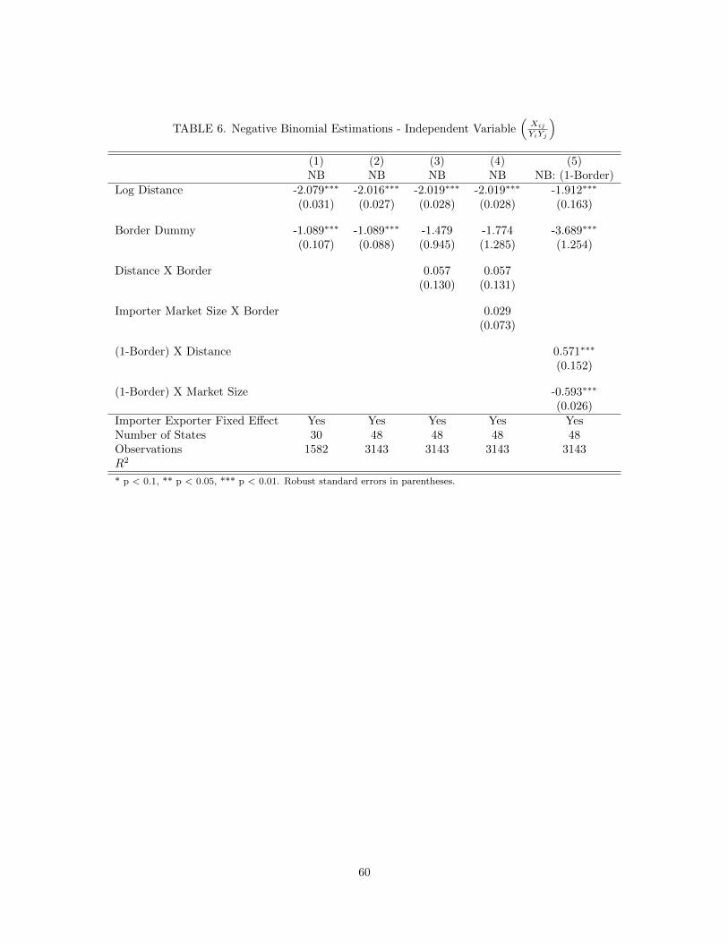
TABLE 6. Negative Binomial Estimations - Independent Variable(XijYiYj

)(1) (2) (3) (4) (5)NB NB NB NB NB: (1-Border)

Log Distance -2.079∗∗∗ -2.016∗∗∗ -2.019∗∗∗ -2.019∗∗∗ -1.912∗∗∗

(0.031) (0.027) (0.028) (0.028) (0.163)

Border Dummy -1.089∗∗∗ -1.089∗∗∗ -1.479 -1.774 -3.689∗∗∗

(0.107) (0.088) (0.945) (1.285) (1.254)

Distance X Border 0.057 0.057(0.130) (0.131)

Importer Market Size X Border 0.029(0.073)

(1-Border) X Distance 0.571∗∗∗

(0.152)

(1-Border) X Market Size -0.593∗∗∗

(0.026)Importer Exporter Fixed Effect Yes Yes Yes Yes YesNumber of States 30 48 48 48 48Observations 1582 3143 3143 3143 3143R2


60

TABLE 7. Summary Statistics for Internal Distance by Product

mean max min sd countBarley 1706 2217 1526 307 7Grain 1006 2644 606 570 50Maize 1448 3486 840 452 96Oats 1797 2567 1094 463 19Potatoes 2148 3121 1561 564 29Rice 1592 3536 859 642 99Soy 1459 2655 932 408 44Tobacco 898 3526 510 555 41Tomatoes 2648 3252 821 857 16Wheat 1628 2162 1107 273 78Total 1515 3536 510 630 479

All numbers are reported in miles.

TABLE 8. Products Included in Sample

HS Code Description Non-IV Sample IV Sample0701 Potatoes (except sweet potatoes), fresh or chilled Yes Yes0702 Tomatoes, fresh or chilled Yes Yes0708 Leguminous vegetables, shelled or not, fresh or chilled Yes No0805 Citrus fruit, fresh or dried Yes No0806 Grapes, fresh or dried Yes No0808 Apples, pears, and quinces, fresh Yes No0809 Apricots, cherries, peaches, plums & sloes, fresh Yes No1001 Wheat and meslin Yes Yes1003 Barley Yes Yes1004 Oats Yes Yes1005 Corn (maize) Yes Yes1006 Rice Yes Yes1007 Grain sorghum Yes Yes1201 Soybeans, whether or not broken Yes Yes1202 Peanuts (ground-nuts), raw Yes No1206 Sunflower seeds, whether or not broken Yes No1214 Rutabagas, hay, clover & other forage products Yes No2401 Tobacco, unmanufactured Yes Yes

61

62

TABLE 9. Internal Distance Gravity Regressions

(1) (2) (3) (4)

Basic Reg, No IV Basic Reg, 2SLS Controls Reg, No IV Controls Reg, 2SLS

Log of External Distance -1.053∗∗ -1.068∗∗∗ -0.445 -0.465∗

(0.382) (0.211) (0.415) (0.262)

Log of Internal Distance -1.936∗∗∗ -1.669∗∗∗ -2.002∗∗∗ -1.754∗∗∗

(0.479) (0.504) (0.518) (0.497)

Log of Importer GDP 0.533∗∗∗ 0.538∗∗∗ 0.431∗∗∗ 0.433∗∗∗

(0.086) (0.057) (0.074) (0.073)

Contiguity Dummy 1.796 1.772∗∗

(1.039) (0.759)

Common Language Dummy -0.294 -0.318

(0.274) (0.272)

Log of Importer Area 0.012 0.014

(0.087) (0.064)

Colonial Dummy 0.411 0.408

(0.564) (0.475)

RTA Dummy 1.010∗ 1.002∗∗∗

(0.529) (0.337)

Common Currency Dummy 0.476 0.467

(0.565) (0.607)

Fixed Effects Used Commodity Commodity Commodity Commodity

Observations 479 479 479 479

R2 0.241 0.240 0.274 0.274

First-stage F-stat 400.859 403.439

P-value of test ln intdist 6= ln dist 0.272 0.292 0.100 0.031


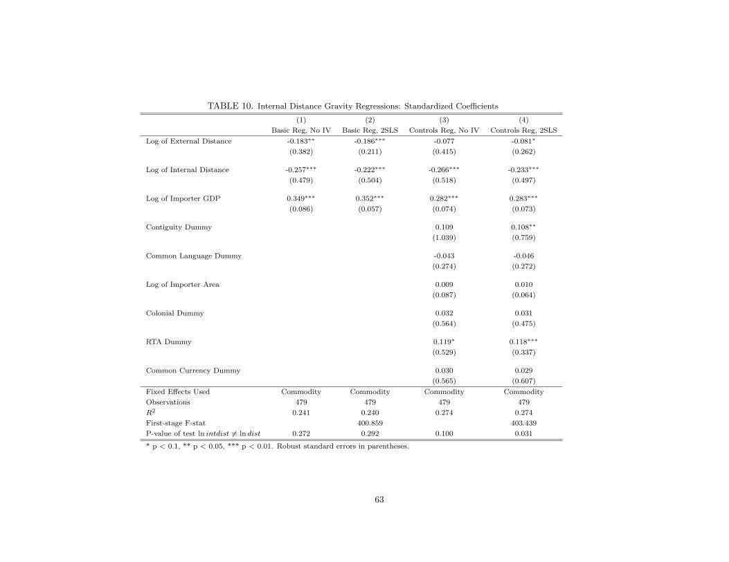
63

TABLE 10. Internal Distance Gravity Regressions: Standardized Coefficients

(1) (2) (3) (4)

Basic Reg, No IV Basic Reg, 2SLS Controls Reg, No IV Controls Reg, 2SLS

Log of External Distance -0.183∗∗ -0.186∗∗∗ -0.077 -0.081∗

(0.382) (0.211) (0.415) (0.262)

Log of Internal Distance -0.257∗∗∗ -0.222∗∗∗ -0.266∗∗∗ -0.233∗∗∗

(0.479) (0.504) (0.518) (0.497)


(0.086) (0.057) (0.074) (0.073)

Contiguity Dummy 0.109 0.108∗∗

(1.039) (0.759)

Common Language Dummy -0.043 -0.046

(0.274) (0.272)

Log of Importer Area 0.009 0.010

(0.087) (0.064)

Colonial Dummy 0.032 0.031

(0.564) (0.475)

RTA Dummy 0.119∗ 0.118∗∗∗

(0.529) (0.337)

Common Currency Dummy 0.030 0.029

(0.565) (0.607)

Fixed Effects Used Commodity Commodity Commodity Commodity

Observations 479 479 479 479

R2 0.241 0.240 0.274 0.274

First-stage F-stat 400.859 403.439

P-value of test ln intdist 6= ln dist 0.272 0.292 0.100 0.031


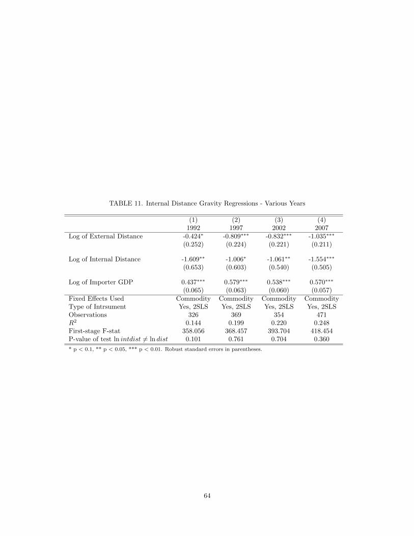
TABLE 11. Internal Distance Gravity Regressions - Various Years

(1) (2) (3) (4)1992 1997 2002 2007

Log of External Distance -0.424∗ -0.809∗∗∗ -0.832∗∗∗ -1.035∗∗∗

(0.252) (0.224) (0.221) (0.211)

Log of Internal Distance -1.609∗∗ -1.006∗ -1.061∗∗ -1.554∗∗∗

(0.653) (0.603) (0.540) (0.505)


(0.065) (0.063) (0.060) (0.057)Fixed Effects Used Commodity Commodity Commodity CommodityType of Intrsument Yes, 2SLS Yes, 2SLS Yes, 2SLS Yes, 2SLSObservations 326 369 354 471R2 0.144 0.199 0.220 0.248First-stage F-stat 358.056 368.457 393.704 418.454P-value of test ln intdist 6= ln dist 0.101 0.761 0.704 0.360


64

TABLE 12. Trade Creation and Trade Diversion in the E.U.

(1) (2) (3) (4)EU Border Effect Market Size Effect EU Border Effect EU Border Effect

EU to EU trade 0.234∗∗∗ 2.312∗∗∗ 0.938∗∗∗ 0.187∗

(0.042) (0.402) (0.064) (0.107)

EU to Non-EU trade -0.149∗∗∗ 0.164 0.348∗∗∗ -0.079(0.024) (0.164) (0.040) (0.066)

Euro to Euro trade -0.074 0.009 0.194∗∗

(0.052) (0.054) (0.093)

Importer GDP * EU to EU dummy -0.074∗∗∗

(0.023)

Exporter GDP * EU to EU dummy -0.099∗∗∗

(0.025)

Importer GDP * EU to non-EU dummy -0.027∗∗

(0.011)

Exporter GDP * EU to non-EU dummy -0.001(0.012)

Sample all all Eastern Bloc ScandinaviaObservations 532017 532017 45994 34480Fixed Effects Importer-Exporter Importer-Exporter Importer-Exporter Importer-ExporterTime Fixed Effects Yes Yes Yes YesR2 0.105 0.105 0.106 0.090


65

TABLE 13. Individual Trade Creation and Trade Diversion Effects

(1) (2) (3) (4)Country EU to EU EU to EU Standard Error EU to Non-EU EU to Non-EU Standard ErrorAustria -0.126 0.122 -0.220 0.084Bulgaria 1.063 0.129 0.569 0.085Cyprus 0.503 0.152 0.032 0.010CzechRep 0.110 0.142 0.031 0.086Denmark 0.742 0.181 0.248 0.089Estonia 0.355 0.163 0.219 0.106Finland -0.130 0.154 -0.038 0.089Greece -0.869 0.166 -0.740 0.101Hungary 0.798 0.154 -0.009 0.091Ireland 0.475 0.191 0.193 0.120Latvia 0.636 0.205 0.245 0.114Lithuania -0.165 0.204 -0.295 0.129Malta 0.677 0.172 0.329 0.099Poland 1.122 0.129 0.375 0.082Portugal -0.012 0.186 -0.310 0.089Romania 0.913 0.170 -0.057 0.110Slovakia 0.647 0.165 0.315 0.107Slovenia 0.398 0.180 0.248 0.125Spain -0.295 0.150 -0.459 0.072Sweden -0.125 0.131 -0.301 0.086UK 0.492 0.170 0.111 0.090

66

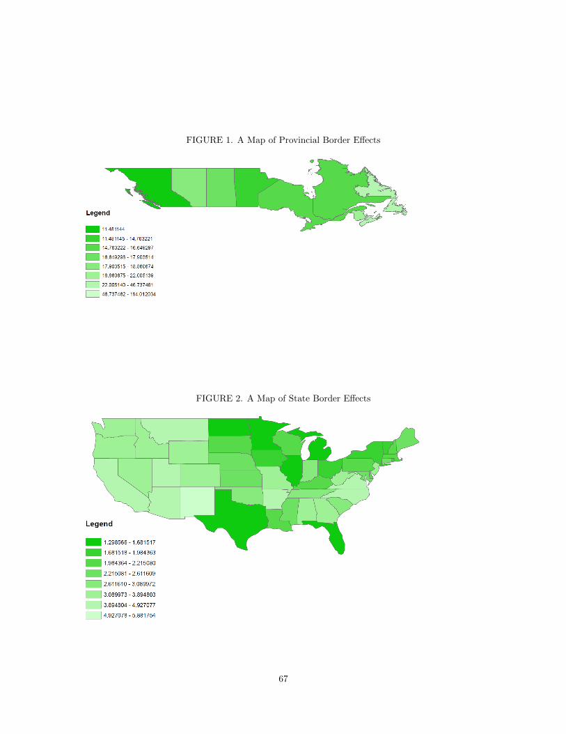
FIGURE 1. A Map of Provincial Border Effects

FIGURE 2. A Map of State Border Effects

67

FIGURE 3. Graph of the Implied Border Effect Over Various Importer Market Sizes

68

FIGURE 4. Imports and Exports Before and After Joining the EU - Austria and Bulgaria

69

FIGURE 5. Imports and Exports Before and After Joining the EU - Cyprus and Czech Rep.

70

FIGURE 6. Imports and Exports Before and After Joining the EU - Denmark and Estonia

71

FIGURE 7. Imports and Exports Before and After Joining the EU - Finland and Greece

72

FIGURE 8. Imports and Exports Before and After Joining the EU - Hungary and Ireland

73

FIGURE 9. Imports and Exports Before and After Joining the EU - Latvia and Lithuania

74

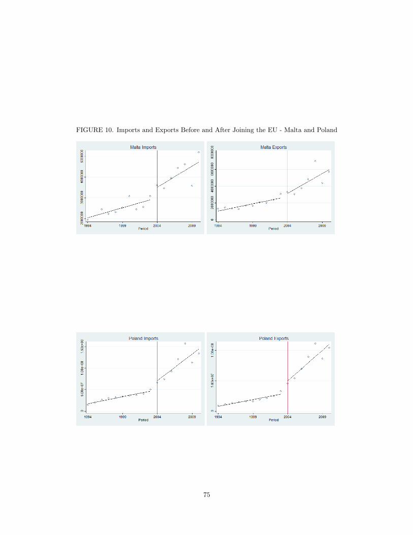
FIGURE 10. Imports and Exports Before and After Joining the EU - Malta and Poland

75

FIGURE 11. Imports and Exports Before and After Joining the EU - Portugal and Romania

76

FIGURE 12. Imports and Exports Before and After Joining the EU - Slovakia and Slovenia

77

FIGURE 13. Imports and Exports Before and After Joining the EU - Spain and Sweden

78

FIGURE 14. Imports and Exports Before and After Joining the EU - United Kingdom

79

REFERENCES CITED

Agnosteva, D. E., Anderson, J. E., and Yotov, Y. V. (2014). Intra-national Trade Costs:Measurement and Aggregation. (19872).

Anderson, J. and van Wincoop, E. (2003). Gravity with Gravitas: A Solution to the BorderPuzzle. American Economic Review, 93(1):170–192.

Anderson, J. E. (1979). A Theoretical Foundation for the Gravity Equation. The AmericanEconomic Review, 69(1):106–116.

Anderson, J. E. and Van Wincoop, E. (2004). Trade Costs.

Anderson, J. E. and Yotov, Y. V. (2010). The Changing Incidence of Geography. The AmericanEconomic Review, 100(5):2157–86.

Arkolakis, C. (2010). Market Penetration Costs and the New Consumers Margin in InternationalTrade. Journal of political economy, 118(6):1151–1199.

Atkin, D. and Donaldson, D. (2014). Who is Getting Globalized? The Size and Implications ofIntranational Trade Costs.

Baier, S. L. and Bergstrand, J. H. (2004). Economic Determinants of Free Trade Agreements.Journal of International Economics, 64(1):29–63.

Baier, S. L. and Bergstrand, J. H. (2007). Do Free Trade Agreements Actually Increase Members’International Trade? Journal of international Economics, 71(1):72–95.

Baier, S. L. and Bergstrand, J. H. (2009). Bonus vetus OLS: A Simple Method for ApproximatingInternational Trade-cost Effects Using the Gravity Equation. Journal of InternationalEconomics, 77(1):77–85.

Balistreri, E. J. and Hillberry, R. H. (2007). Structural Estimation and the Border Puzzle.Journal of International Economics, 72(2):451–463.

Bernard, A. B. and Jensen, B. J. (1999). Exceptional Exporter Performance: Cause, Effect, orBoth? Journal of International Economics, 47(1):1–25.

Blonigen, B. A. and Wilson, W. W. (2006). International Trade, Transportation Networks, andPort Choice. http://www. nets. iwr. usace. army.mil/docs/PortDevInternalTransport/PortChoice114. pdf.

Blonigen, B. A. and Wilson, W. W. (2008). Port Efficiency and Trade Flows. Review ofInternational Economics, 16(1):21–36.

Burlando, A., Cristea, A., and Lee, L. M. (Mimeo, 2014). The Trade Consequences of MaritimeInsecurity: Evidence from Somali Piracy.

Campbell, J. R. and Hopenhayn, H. A. (2005). Market Size Matters. The Journal of IndustrialEconomics, 53(1):1–25.

Chaney, T. (2008). Distorted Gravity: The Intensive and Extensive Margins of InternationalTrade. The American Economic Review, 98(4):1707–1721.

Chen, N. (2004). Intra-national Versus International Trade in the European Union: Why DoNational Borders Matter? Journal of International Economics, 63(1):93–118.

80

Clark, X., Dollar, D., and Micco, A. (2004). Port Efficiency, Maritime Transport Costs, andBilateral Trade. Journal of development economics, 75(2):417–450.

Cosar, A. K. and Demir, B. (2014). Domestic Road Infrastructure and International Trade:Evidence from Turkey.

Cosar, A. K. and Fajgelbaum, P. D. (Mimeo, 2014). Internal Geography, International Trade, andRegional Outcomes. University of Chicago and UCLA, unpublished mimeo.

Costinot, A. and Donaldson, D. (2011). How Large Are the Gains from Economic Integration?Theory and Evidence from US Agriculture, 1880-2002.

Coughlin, C. C. and Novy, D. (2011). Domestic and International Border Effects: State SizeMatters.

Dias, D. (2011a). Gravity and Globalization.

Dias, D. (2011b). The Border Effect Through the Rearview Mirror: Would the Puzzle HaveExisted if Todays Tools Had Been Used?

Disdier, A.-C. and Head, K. (2008). The Puzzling Persistence of the Distance Effect on BilateralTrade. The Review of Economics and Statistics, 90(1):37–48.

Eaton, J. and Kortum, S. (2002). Technology, Geography, and Trade. Econometrica,70(5):1741–1779.

Eaton, J., Kortum, S., and Kramarz, F. (2011). An Anatomy of International Trade: Evidencefrom French Firms. Econometrica, 79(5):1453–1498.

Engel, C. and Rogers, J. H. (1996). How Wide Is the Border? The American Economic Review,86(5):1112–1125.

FAO and IIASA (2010). Global Agro-ecological Zones (GAEZ v3.0). FAO, Rome, Italy andIIASA, Laxenburg, Austria.

Feenstra, R. (2003). Border Effects and the Gravity Equation: Consistent Methods forEstimation. Scottish Journal of Political Economy, 49(5):491–506.

Glick, R. and Rose, A. K. (2002). Does a Currency Union Affect Trade? The Time-seriesEvidence. European Economic Review, 46(6):1125–1151.

Gorodnichenko, Y. and Tesar, L. L. (2009). Border Effect or Country Effect? Seattle May Not Beso Far from Vancouver After All. American Economic Journal, Macroeconomics,1(1):219–241.

Haveman, J. and Hummels, D. (1998). Trade Creation and Trade Diversion: New EmpiricalResults. Journal of Transnational Management Development, 3(2):47–72.

Head, K., Mayer, T., and Ries, J. (2010). The Erosion of Colonial Trade Linkages AfterIndependence. Journal of International Economics, 81(1):1–14.

Helliwell, J. F. (1998). How Much Do National Borders Matter?

Helpman, E., Melitz, M., and Rubinstein, Y. (2008). Estimating Trade Flows: Trading Partnersand Trading Volumes. The Quarterly Journal of Economics, 123(2):441–487.

Hillberry, R. and Hummels, D. (2003). Intranational Home Bias: Some Explanations. Review ofEconomics and Statistics, 85(4):1089–1092.

81

Hillberry, R. and Hummels, D. (2008). Trade Responses to Geographic Frictions: ADecomposition Using Micro-data. European Economic Review, 52(3):527–550.

Hummels, D. and Schaur, G. (2013). Time as a Trade Barrier. The American Economic Review,103(7):2935–59.

Krugman, P. (1980). Scale Economies, Product Differentiation, and the Pattern of Trade. TheAmerican Economic Review, 70(5):950–959.

Krugman, P. (1991). The Move Toward Free Trade Zones. Economic Review, 76(6):5.

Magee, C. S. (2008). New Measures of Trade Creation and Trade Diversion. Journal ofInternational Economics, 75(2):349–362.

Malchow, M. B. and Kanafani, A. (2004). A Disaggregate Analysis of Port Selection.Transportation Research Part E: Logistics and Transportation Review, 40(4):317–337.

Matsuo, M. and Ishise, H. (2012). The US-Canada Border Effect: Smaller Than PreviouslyThought and Becoming Smaller.

McCallum, J. (1995). National Borders Matter: Canada-US Regional Trade Patterns. TheAmerican Economic Review, 85(3):615–623.

Melitz, M. J. (2003). The Impact of Trade on Intra-industry Reallocations and AggregateIndustry Productivity. Econometrica, 71(6):1695–1725.

Millimet, D. L. and Osang, T. (2007). Do State Borders Matter for US Intranational Trade? TheRole of History and Internal Migration. Canadian Journal of Economics/Revue canadienned’economique, 40(1):93–126.

Nitsch, V. (2000). National Borders and International Trade: Evidence from the European Union.Canadian Journal of Economics/Revue canadienne d’economique, 33(4):1091–1105.

Nitsch, V. (2002). Honey, I Shrunk the Currency Union Effect on Trade. The World Economy,25(4):457–474.

Nunn, N. and Qian, N. (2011). The Potato’s Contribution to Population and Urbanization:Evidence from a Historical Experiment. The Quarterly Journal of Economics, 126:593–650.

Obstfeld, M. and Rogoff, K. (2001). The Six Major Puzzles in International Macroeconomics: IsThere a Common Cause? pages 339–412.

Parsley, D. C. and Wei, S.-J. (2001). Explaining the Border Effect: the Role of Exchange RateVariability, Shipping Costs, and Geography. Journal of International Economics,55(1):87–105.

Query, J. (2014). Market Size and Heterogeneity of Border Effects in Gravity Models of Trade.

Rauch, J. E. and Trindade, V. (2002). Ethnic Chinese Networks in International Trade. Review ofEconomics and Statistics, 84(1):116–130.

Redding, S. and Venables, A. J. (2004). Economic Geography and International Inequality.Journal of international Economics, 62(1):53–82.

Redding, S. J. and Turner, M. A. (2014). Transportation Costs and the Spatial Organization ofEconomic Activity. Chapter in progress for the Handbook of Regional and UrbanEconomics.

82

Rose, A. K. (2000). One Money, One Market: the Effect of Common Currencies on Trade.Economic policy, 15(30):7–46.

Silva, J. S. and Tenreyro, S. (2006). The Log of Gravity. The Review of Economics and Statistics,88(4):641–658.

Taylor, J. C., Robideaux, D. R., and Jackson, G. C. (2004). US-Canada Transportation andLogistics: Border Impacts and Costs, Causes, and Possible Solutions. TransportationJournal, 43(4):5–21.

Tinbergen, J. (1962). Shaping the World Economy: Suggestions for an International EconomicPolicy.

Viner, J. (1950). The Customs Union Issue.

Volpe Martincus, C. and Blyde, J. (2013). Shaky Roads and Trembling Exports: Assessing theTrade Effects of Domestic Infrastructure Using a Natural Experiment. Journal ofInternational Economics, 90(1):148–161.

Wolf, H. C. (2000). Intranational Home Bias in Trade. Review of Economics and Statistics,82(4):555–563.

Wolf, N. (2005). Path Dependent Border Effects: the Case of Polands Reunification (1918–1939).Explorations in Economic History, 42(3):414–438.

Wonnacott, P. and Lutz, M. (1989). Is There a Case for Free Trade Areas? Free Trade Areas andUS Trade Policy, 59:84.

83

the impact of transportation costs and trade barriers …

Documents