1

The impact of unconventional monetary policy on firm financing constraints: Evidence from the maturity extension program

Nathan Foley-Fisher, Rodney Ramcharan, and Edison Yu1

Federal Reserve Board     University of Southern California   Federal Reserve Bank of Philadelphia 

December 2015 

Abstract 

This paper investigates the impact of unconventional monetary policy on firm financing

constraints. It focuses on the Federal Reserve’s maturity extension program (MEP),

intended to lower longer-term rates and flatten the yield curve by reducing the supply of

long-term government debt. Consistent with those models that emphasize bond market

segmentation and limits to arbitrage, around the MEP’s announcement, stock prices rose

most sharply for those firms that are more dependent on longer-term debt. These firms

also issued more long-term debt during the MEP and expanded employment and

investment. These responses are most pronounced for those firms that are larger and older,

and hence less likely to be financially constrained. There is also evidence of “reach for

yield” behavior among some institutional investors, as the demand for riskier debt also

rose during the MEP. Our results suggest that unconventional monetary policy might have

helped to relax financing constraints and stimulate economic activity in part by inducing

gap-filling behavior and affecting the pricing of risk in the bond market.

JEL: E52, G23, G32 

Key words: unconventional monetary policy, firm‐financing constraints, bond markets.  

 

 

                                                            

1 Nathan.C.Foley‐Fisher@frb.gov; rramchar@usc.edu; Edison.Yu@phil.frb.org. We would like to thank Roc Armenter, Mitchell Berlin, Jef Boeckx, Pablo D'Erasmo, Harry DeAngeleo, Thorsten Drautzburg, Steven Sharpe, Ashley Wang, and participants in seminars hosted by the Bundesbank, Federal Reserve Bank of Philadelphia, Federal Reserve Board of Governors. The views expressed in this paper are those of the authors and do not necessarily reflect the views of the Federal Reserve Bank of Philadelphia, the Federal Reserve Board of Governors, or the Federal Reserve System. 

  2

 

1.  Introduction 

To help overcome the zero lower bound constraint after the 2008‐2009 financial crisis, the 

Federal Reserve and other central banks have implemented a number of unconventional policies, 

including a series of large‐scale asset purchases or quantitative easing (QE). These policies are in part 

intended to work around the zero lower bound constraint by directly buying assets, such as U.S. 

Treasury bonds and mortgage‐backed securities, in order to offset disruptions in private sector 

intermediation and stimulate economic activity (Cahill et al., 2013; Gertler and Karadi, 2011; 

Krishnamurthy and Vissing‐Jorgensen, 2011; and Shleifer and Vishny, 2011).2 

This paper develops a number of empirical tests to understand better the impact of 

unconventional monetary policy. We focus mainly on the Federal Reserve’s attempt to flatten the yield 

curve through the maturity extension program (MEP), announced on Sept. 21, 2011. The explicit 

intention behind the MEP was to reduce the supply of long‐term Treasury securities and put downward 

pressure on longer‐term interest rates, especially on those assets considered close substitutes for long‐

term Treasury securities. Under the plan, lower borrowing costs and increased credit availability would 

relieve possibly binding financing constraints on firms and households. To that end, the MEP committed 

the Federal Reserve to sell about $400 billion in shorter‐term Treasury securities and use the proceeds 

to buy longer‐term Treasury securities. The Federal Reserve extended the program in June 2012 through 

December 2012 for an additional $267 billion. In this paper, we examine how stock prices, debt issuance, 

and firms' investment and hiring activities reacted to the MEP. 

Our empirical tests of the MEP’s impact are motivated by those theories that emphasize partial 

segmentation in bond markets, limits to arbitrage, and the role of nonfinancial corporations in 

responding to shocks in the supply of government debt (Greenwood, Hanson, and Stein, 2010; Vayanos 

and Vila, 2009). Partial segmentation in bond markets can arise when some natural buyers of bonds, 

such as insurance firms and pension funds, prefer investing at specific maturities; life insurers, for 

example, mainly invest in longer‐term bonds to match the duration of their liabilities.3 These models 

also observe that in response to an unexpected decline in the supply of longer‐term government debt, 

arbitrageurs with limited capital relative to the size of the shock or high levels of risk aversion may only 

                                                            

2 See Chowdorow‐Reich (2013) for evidence on how the crisis might have affected financing constraints at bank‐

dependent firms. Di Maggio and Kacperczyk (2014) study the impact of low interest rates on reach for yield 

behavior in the mutual fund industry. Benmelech, Meisenzahl, and Ramcharan (2014) and Ramcharan, Verani, and 

Van den Heuvel (forthcoming) study the impact of financial sector distress during the crisis on households. 

DiMaggio, Kermani, and Ramcharan (2014) and Keys et. al (2014) study how monetary policy after the crisis might 

have affected household level financing constraints.  

3 The average maturity of corporate bond holdings in the life insurance industry about 11 years, roughly 

unchanged since 2004 (NAIC 2014).   

  3

imperfectly enforce the expectations hypothesis, resulting in bond yields that differ from the 

expectations hypothesis.4  

With inelastic demand and limits to arbitrage, the argument in Greenwood, Hanson, and Stein 

(2010) predicts that nonfinancial corporations would fill in the supply gaps for longer‐term debt created 

by government supply shocks like the MEP.5 This channel would be especially strong for those firms with 

a preference for using longer‐term debt to meet their financing needs or those with the financial 

flexibility to adjust the maturity of their debt issuances easily. Moreover, if these firms faced binding 

financing constraints after the crisis, then filling the supply gaps created by the MEP might also allow 

them to take better advantage of growth opportunities, leading to increased investment and 

employment. In contrast, if arbitrageurs operate freely at different maturities along the yield curve, then 

any policy‐induced reduction in longer‐term yields might be evanescent, leaving little impact on 

corporate debt issuances and real outcomes. 

Table 1 shows that the decline in the supply of longer‐term government debt envisaged by the 

MEP was large relative to the size of the Treasury market, and we find evidence consistent with the gap‐

filling hypothesis in Greenwood, Hanson, and Stein (2010). Our first set of tests exploits cross‐sectional 

differences in the stock price response to the MEP’s announcement. These tests suggest that market 

participants likely expected the MEP to lower financing costs and relax financing constraints primarily 

for those firms that traditionally rely on longer‐maturity debt. That is, abnormal stock returns on the day 

after the MEP’s announcement rose sharply for those nonfinancial firms that traditionally relied on 

longer‐term debt finance. An increase of one standard deviation in the long‐term debt ratio of a firm is 

associated with a 0.26 percentage point higher abnormal return, which is about 93% in annualized terms. 

These results are robust to a variety of controls and persist even when using higher‐frequency intraday 

data around the announcement. 

The next set of tests examines the response of firms to the MEP using a difference‐in‐difference 

methodology. There is evidence that firms with a greater preference for relying on longer‐term debt 

issued more longer‐term debt during the MEP to fill the “gap” created by the Fed’s purchases of longer‐

term assets. An increase of one standard deviation in the long‐term debt ratio is associated with about a 

8% faster growth in the stock of long‐term debt during the MEP’s implementation. As a falsification test, 

the coefficient estimate for the growth in short‐term debt is not statistically significant, giving us some 

confidence that the effect of the MEP program operates through longer‐term borrowing. And consistent 

with the gap‐filling motive, as well as the evidence in Badoer and James (forthcoming), we find that 

                                                            

4 What makes bond financing even more important during the financial crisis is that there is evidence of firms 

switching from bank financing to bond financing during the period (see De Fiore and Uhlig, 2015). Various reports 

on this can also be found on the Bankscope platform.  

5 Apart from the MEP, Badoer and James (forthcoming) provide evidence that gap‐filling behavior in response to 

Treasury supply shocks might be an important determinant of long‐term corporate issuances. 

  4

firms with more financial flexibility might have more easily adjusted their financing plans to take 

advantage of the MEP.  

Beyond inducing gap‐filling bond issuances by nonfinancial firms, low nominal interest rates or 

the expectation that low rates might persist can also create incentives for certain types of creditors to 

take added risk in an effort to reach for yield, affecting risk premia and the demand for longer‐dated 

high‐yielding debt (Morris and Shin, 2012; Borio and Zhu, 2012; and Hanson and Stein, forthcoming). 

That is, a monetary policy shock such as the MEP might be associated with changes in the risk premium 

over and above any change in the actuarially fair long‐term interest rate implied by the expectations 

theory of the yield curve.  

We test this “reach for yield” channel using a discontinuity in the capital regulations that govern 

the insurance industry (Becker and Ivashina, forthcoming). Insurers are the main buyers of corporate 

debt in the United States, accounting for about 60% of all institutional investors’ corporate bond 

holdings. Their bond holdings are also subject to risk‐adjusted capital requirements. These requirements 

are based on bond ratings, and they increase exponentially as the credit quality worsens. For bonds 

rated AAA through A‐, the capital requirement is identical, but this requirement rises sharply for bonds 

below the A‐ threshold. Among AAA through A‐ bonds, we show that during the period of the MEP’s 

implementation, risk premia fell disproportionately for the higher‐yielding A‐ bonds, reflecting in part an 

increase demand for higher‐yielding debt that also economize on regulatory capital requirements. We 

also find evidence that those insurers more dependent on income earned from Treasury securities 

before the MEP, and thus more affected by the decline in longer‐term Treasury yields, increased their 

relative purchases of higher yielding A‐ securities during the MEP’s implementation. 

Finally, we investigate the MEP’s impact on a range of firm decisions. The difference‐in‐

difference approach suggests that firms more dependent on longer‐term debt may have been able to 

take advantage of the more benign financing conditions to increase investment and employment during 

the MEP relative to other periods. During the MEP’s implementation, an increase of one standard 

deviation in long‐term debt dependence is associated with a 1.4 percentage point increase in 

employment growth during the MEP. The effects are similar for the growth in plant and equipment 

expenditures. And again consistent with the prediction in Greenwood, Hanson, and Stein (2010), these 

magnitudes appear larger for firms with stronger balance sheets and more financial flexibility.  

Our analysis contributes to the literature in three ways. First, we provide new evidence that 

nonfinancial corporations, especially those that are larger and older and thus less likely to be financially 

constrained, might systematically provide liquidity in response to shocks in the supply of government 

debt. Second, some of our results inform the broader literature on the impact of external financing 

constraints on stock returns—see, for example, Whited and Wu (2006). Third, this paper adds to the 

debate on the effects of unconventional policies such as the MEP. Some have argued, for example, that 

these policies might have little real impact, as economic growth in a post‐crisis economy might be 

shaped more by the pace of reallocation across geography and industries (King, 2013). Unconventional 

policies are then more likely instead to fuel asset price bubbles, excessive risk‐taking, and future 

instability (Rajan, 2013; Stein, 2014). Several recent papers already provide important evidence 

  5

documenting the effects of these policies, primarily around their announcement dates, on a range of 

asset prices.6 But we are able to probe further and build upon economic theory to identify key 

mechanisms through which the MEP might relax financing constraints and affect economic decisions at 

firms.  

The remainder of the paper is structured as follows: Section II describes the maturity extension 

program and the basic empirical tests. Section III provides a summary of data used in the paper. Section 

IV presents empirical results using firm‐ and bond‐level data. Section V concludes. 

2. The Maturity Extension Program and the Basic Hypotheses 

The Federal Reserve announced the maturity extension program (MEP) at 2:23 p.m. EST on Sept. 

21, 2011, in its Federal Open Market Committee (FOMC) statement. The Federal Reserve announced 

that it would sell or redeem a total of $400 billion of shorter‐term Treasury securities and use the 

proceeds to buy longer‐term Treasury securities, thereby extending the average maturity of the 

securities in the Federal Reserve’s portfolio. With the short‐term interest rate near the zero lower 

bound, the program’s intention was to lower long‐term interest rates, and ultimately the cost of longer‐

term credit for households and firms.7 The September 2011 announcement indicated a program end 

date of June 2012. But in June 2012, the MEP was renewed; the Fed announced plans to swap another 

$200 billion in short‐term Treasuries for longer‐maturity debt. The MEP was officially discontinued at 

the end of 2012. 

The MEP was large relative to the size of the Treasury market. Table 1 shows the maturity 

structure of the Federal Reserve Bank of New York purchases of Treasuries under the MEP. The bottom 

panel of the table also shows the stock of outstanding Treasuries at various maturities at the end of 

2011. For bonds of duration roughly eight years or longer, projected MEP purchases equal about 18 

percent of the outstanding stock Treasuries in 2011. To help visualize the potential impact of these 

purchases on bond prices, panel A of Figure 1 plots the daily yields of 30‐year and one‐year Treasury 

bonds around the announcement of MEP. The solid line is the yield on the 30‐year Treasury and the 

dashed line is the one‐year yield. The 30‐year yield started to drop when the Fed announced the MEP on 

Sept. 21, 2011, but the more significant drop occurred on Sept. 22, 2011. Consistent with the economic 

magnitudes in Table 1, the drop of 25 basis points on Sept. 22 alone was a two standard deviation 

change, and the 30‐year yield dropped by 42 basis points over the two‐day period.  

                                                            

6 See, for example, Cahil et al., 2013; Gagnon et al., 2011; Hamilton and Wu, 2012; Swanson and Williams 

(forthcoming), and Wright, 2012. 

7 See the following link for details about the MEP

(www.federalreserve.gov/monetarypolicy/maturityextensionprogram-faqs.htm).  

  6

Intraday movements in yields show the MEP’s impact more clearly. Panel B of Figure 1 plots the 

cumulative change in the 30‐year Treasury yield over Sept. 21 and 22, observed at 30‐minute intervals. 

Yields began dropping right after the announcement at 2:30 p.m. on Sept. 21. But consistent with the 

fact that market participants might have taken time to process the announcement’s implications, as well 

as the fact that the Federal Reserve Bank of New York’s trading desk only began program 

implementation at 9:30 a.m. on Sept. 22, yields continued falling until the afternoon of Sept. 22. Panel C 

shows that the yield curve of Treasury bonds also tilted downward, consistent with the intention of the 

MEP. The solid line is the yield curve of Treasury bonds on Sept. 20, 2011. The dashed and dotted lines 

are the yield curves for Sept. 21 and Sept. 22, 2011, respectively.  

Models that emphasize bond market segmentation and limited arbitrage suggest that the MEP 

might affect the term spread and the pattern of corporate debt issuances (Greenwood, Hanson, and 

Stein, 2010; Vayanos and Vila, 2009). If arbitrageurs are risk averse, and some natural buyers of 

corporate debt have relatively inelastic demand for longer‐dated maturities, perhaps because they wish 

to match the maturities of their assets and liabilities, then targeted policies such as the MEP can flatten 

the yield curve. A key implication of these theories then is that those firms with a “preferred habitat” or 

a preference for longer‐term liabilities, or those able to adjust easily the maturity structure of their 

borrowings, are likely to benefit the most from the MEP’s attempt to reduce the relative cost of longer‐

term external finance.  

But unconventional policies such as the MEP can also affect the demand for debt and the risk 

premia that borrowers might face. The expectation that low rates might persist can induce certain types 

of creditors to take added risk in an effort to reach for yield, reducing risk premia (Guerrieri and Kondor, 

2012; Hanson and Stein, forthcoming; and Stein, 2013). Investors, for example, with a focus on current 

income and a need to hold longer‐term assets to match the duration of their liabilities, such as life 

insurance firms, could rebalance their portfolios in favor of both more duration and credit risk when 

they expect longer‐term interest rates to remain low for an extended period.8 In this case, bond market 

risk premia are likely to decline especially for those firms that issue longer‐term debt. 

Motivated by these ideas of limited arbitrage and segmentation at various points in the yield 

curve, we construct a number of tests to measure the MEP’s impact. These tests build on the idea that 

in a cross‐section of firms, the policy’s impact should be the largest among those firms with a stronger 

preference for issuing longer‐term maturities. When applied to an event study framework around the 

MEP’s announcement, if market participants absorbed the forward guidance associated with the MEP 

and believed in segmentation and limits to arbitrage, then stock prices of firms with a higher 

dependence on long‐term debt should react more positively to the MEP’s announcement. After all, 

because the expected effect of the MEP was to relax financing constraints disproportionately for these 

types of firms in the aftermath of the financial crisis, they would now be better able to take advantage 

of growth opportunities.  

                                                            

8 Morris and Shin (2012) develop a variation of this idea in the case of asset managers, noting that herding 

behavior can lead to a collapse in the risk premium after a central bank signals low future rates.  

  7

The second battery of tests focuses on external finance. If the MEP disproportionately reduced 

the cost of external finance for these firms, we should see an increase in their debt issuances at the 

extensive margin during the program’s implementation relative to other types of firms. We use a 

difference‐in‐difference framework to test these predictions. We also construct tests to gauge the 

impact of the MEP on the search for yield behavior among the natural buyers of long dated debt, and 

study its impact on bond market risk premia and the portfolios of insurance companies. A final set of 

tests is motivated by the idea that if the MEP did relax financing constraints disproportionately for those 

firms better able to fill the gap in longer‐term debt, then these firms might more readily expand 

employment and investment during the program relative to other types of firms.  

The MEP provides an especially useful context in which to investigate the effects of 

unconventional monetary policy on real economic outcomes. The relative calm around the MEP’s 

announcement makes it somewhat easier to avoid conflating the effects of the MEP with wider 

developments in financial markets. The Fed’s previous attempts at quantitative easing, such as QE 1, 

were announced and implemented in 2008 during the financial crisis—a period when financial markets 

were significantly dislocated and the economy was rapidly slowing. This makes it an especially difficult 

period for statistical inference. Panic selling and fire sales in asset markets, as well as general 

uncertainty in the wider economy, all likely occurred around the same time as these unconventional 

monetary policy announcements.  

Compared with the other QE programs, the MEP’s focus was on flattening the yield curve. Even 

though the goal of other QEs was also to stimulate the economy, the MEP had the largest proportion of 

its purchases of long‐maturity securities. This precise focus on the yield curve affords us a “natural 

experiment” to study the differential impact of the program on firms with different debt maturity 

structures, making it somewhat easier to interpret the evidence relative to other monetary policy 

measures during the crisis. Indeed, because movements in the term spread generally reflect broader 

factors, such as expected business cycle movements or consumption smoothing motives, which might 

also shape firm behavior, distinguishing the direct impact of the term spread on firm behavior and asset 

prices from these broader factors can be even more difficult outside of the MEP (Estrella and 

Hardouvelis, 1991; Wheelock and Wohar, 2009).  

To be sure, there are also challenges in interpreting the results using the MEP in our analysis. 

The motivation for the Federal Reserve’s MEP announcement could have been an anticipation of future 

weakness in those sectors more dependent on longer‐term credit. But this anticipatory bias is likely to 

lead to underestimates of the MEP’s impact on asset prices and outcomes for these types of firms. In 

sum, our efforts to identify better the MEP’s impact are aided by the policy’s precise focus on the term 

spread, its well‐defined implementation period, and the relative calm surrounding its announcement. 

However, considerable care is still required when interpreting the evidence. Economic theory 

observes that the asset and liability side of a firm’s balance sheet is jointly determined, and the asset 

side of a firm’s balance sheet could independently shape how a firm might respond to the MEP. For 

instance, because firms might match the maturity of their liabilities with the maturity of their assets, 

those firms that issue longer‐term debt might also operate longer‐lived assets (Myers (1977). In this case, 

  8

changes in the term structure brought about by the MEP could have an independent effect on future 

cash flow and firm value that is separate from the hypothesized external finance channel.  

Also, because of contracting and information problems, a firm’s maturity structure, as well as its 

choice between arm’s‐length and bank financing, can be closely related to the firm’s credit rating, the 

quality of projects chosen by its management, and the information that management might have about 

these projects compared to outsiders (Diamond, 1991; Flannery 1986). 9 But the credit rating of a firm or 

even the market’s perception of the quality of a firm’s projects could also be alternative channels 

through which the MEP might affect firm value. Concretely, a firm with projects that generate variable 

cash flow might both predominantly fund itself with longer‐term debt to reduce the risk of inefficient 

liquidation. It might also expect an increase in demand and higher cash flow on account of a more 

accommodative monetary policy stance. Thus, any increase in firm value that coincides with the MEP’s 

announcement might stem from the expected increase in demand rather than the hypothesized 

relaxation in financing constraints.  

This endogeneity concern guides our empirical research design. In many of our specifications, 

we use a large number of firm‐ and industry‐level observables to control for various aspects of a firm’s 

balance sheet. We also use high‐frequency data to connect more directly our results to the MEP and a 

firm’s dependence on longer‐term debt. We document that those firms more dependent on longer‐term 

debt were also more likely to issue debt during the MEP. And we exploit discontinuities in capital 

regulation among some of the natural buyers of this type of corporate debt to measure the impact of 

the MEP on risk premia and portfolio choices. We also provide evidence that those firms more affected 

by the MEP on account of their capital structure were also more likely to expand employment and 

investment during the program.  

However, it is impossible to address fully this endogeneity concern using firm‐level 

observational data. But by considering a wide range of alternative specifications and developing tests to 

identify the underlying mechanisms through which the MEP might affect firm outcomes, unobserved 

firm heterogeneity is a less attractive interpretation of the evidence, especially when taken together. 

Another concern stems from the fact that most public databases only coarsely measure the maturity 

structure of debt. To help address this measurement problem, we report results based on finer proxies 

for long‐term debt dependence (Rauh and Sufi, 2010). In the next section, we describe the data in 

greater detail. 

                                                            

9 This literature is large, and often points to a nonmonotonic relationship between the choice of maturity structure 

and these firm level observables. See also Hart and Moore,1994; Berglof and von Thadden,1994; the evidence in 

Barclay and Smith,1995; and Guedes and Opler, 1996; as well as the survey in Rajan, 2013 and more recent work 

by Crouzet, 2014. 

  9

3. Data 

We rely on the cross‐firm variation in long‐term debt dependence to construct tests of the 

MEP’s impact. To measure this cross‐firm variation, most of our baseline tests follow Greenwood, 

Hanson, and Stein (2010), and define long‐term debt as debt with a maturity at issuance longer than one 

year. Since these tests depend on the variation across firms in their preference for longer‐term 

maturities relative to shorter‐term debt—see also Badoer and James (forthcoming)—the baseline 

measure of long‐term debt dependence scales long‐term debt by total debt. Also, since the MEP was 

primarily aimed at maturities greater than one year (Table 1), to match better theory and measurement, 

we conduct robustness checks using long‐term debt dependence with the numerator defined as debt 

with remaining maturity in excess of three years.10     

Our choice of control variables is shaped by the fact that the debt maturity structure of a firm 

might be driven by the nature of its assets and the industry in which it operates (see for example Badoer 

and James, forthcoming). We thus include a large number of firm‐level controls from Compustat to limit 

the potential for biased estimates; throughout, financial firms (SIC 6000‐6999) are excluded from the 

sample. These controls include market capitalization, the product of the total number of outstanding 

common shares and the closing stock price at fiscal year end; total assets; the book‐to‐market ratio is 

included to differentiate between growth and value firms and is defined as the ratio of book value of 

equity over market capitalization. We include two measures of firm profitability: 1) net income growth is 

the log growth rate of a firm’s net income; 2) the return on assets is net income divided by total assets; 

we also include operating income before depreciation and normalized by lagged total assets.  

Stock price reaction and debt issuance might also be closely related to investment opportunities, and so 

we include average Q to  control for firms' investment opportunity (see Gan, 2007 and Almeida, 2012 for 

example).  A firm's average Q is the sum of market capitalization and total assets minus book equity, 

normalized by lagged total assets.  We also have a measure of short‐term financing need: The difference 

between accounts receivable and payable, normalized by lagged total sales. Capital intensity measured 

by depreciation divided by lagged total assets is also added as a control variable in the regression. 

Gorodnichenko and Weber (2013) and Barattieri, Basu, and Gottschalk (2014) suggest that capital 

intensity of firms might affect firms’ sensitivity to monetary shocks, since more capital‐intensive firms 

are subject to less wage stickiness, and hence react faster to monetary shocks.  

Again, to limit any spurious associations induced by the crisis, we take the historical average of 

all the control variables through 2007. Some firm‐level variables can vary significantly over time—see, 

for example, the discussion of capital structures in DeAngelo and Roll (2015)—and for robustness, we 

also try taking the average of the control variables through to Sept. 21, 2011, or just use the last 

                                                            

10 Unfortunately, debt reporting becomes increasingly unreliable in Compustat as maturities increase, and 

imputations based on longer maturities are less useful. Please see the data appendix for a discussion of these 

issues.  

  10

available observation before 2007. All variables are winsorized at the 1% level to eliminate outliers. The 

data appendix describes the variables in greater detail.  

Panel A of Table 2 reports summary statistics for two measures of long‐term debt dependence 

and the key control variables. To make more transparent the challenges to casual inference, Panel B of 

Table 2 shows the simple and conditional correlations between the control variables and the baseline 

(one year cutoff) long‐term debt dependence measure. There is some evidence that lower Q, more 

capital intensive and profitable firms tend to depend more on longer‐term debt. In what follows then 

we are careful to include these and a number of other controls in our baseline specification.   

4. The MEP, Long‐Term Debt Dependence, and Stock Returns 

We first examine whether the MEP’s attempt to relax financing constraints affected stock 

returns. That is, if market participants expected the MEP to relax financing constraints primarily for 

those firms that traditionally rely on longer maturity debt, allowing these firms to capitalize better on 

growth opportunities, then abnormal stock returns obtained around the MEP announcement date 

should be positively correlated with a firm’s long‐term debt dependence. But if market participants 

perceived that investors would quickly arbitrage away the MEP’s attempt to reduce longer‐term yields 

relative to shorter‐term debt, leaving little impact on firm financing constraints, then there should be no 

statistically significant relationship between abnormal returns and a firm’s debt maturity profile. These 

tests also rely on the fact that markets did not fully anticipate the MEP. If the MEP details and 

announcement were anticipated, then these anticipation effects should attenuate the impact of the 

MEP announcement on stock returns. 

Broader macroeconomic trends can also mask any potential impact from the MEP’s 

announcement. Long‐term yields began falling in the summer of 2011, driven in part by developments in 

Europe, and well ahead of the MEP’s announcement. If market participants believed that these broader 

macro trends would likely account for most of the movements in yields and firms’ financing costs, then 

the MEP’s announcement would again be expected to have little impact on the abnormal returns of 

those firms more reliant on longer‐term debt.  

   Table 3 examines the relationship between abnormal returns and long‐term debt dependence. 

Column 1 presents the most parsimonious specification: A simple OLS regression of abnormal returns of 

firms on Sept. 22, 2011 on firms' long‐term debt dependence. Abnormal stock returns are obtained from 

a standard one factor model (MacKinlay, 1997), and long‐term debt dependence is defined as the ratio 

of debt with a maturity greater than one year to total debt; for each firm, this ratio is averaged through 

the history of the firm up through Dec. 31, 2006. Throughout, standard errors are clustered at the three‐

digit SIC level. 

Consistent with the preferred habitat hypothesis, and some of the evidence in the literature on 

financing constraints and stock returns—see for example Whited and Wu (2006)—the coefficient 

estimate is positive and statistically significant. A one standard deviation increase in the long‐term debt 

ratio of a firm is associated with a 0.26 percentage point higher abnormal return, which is about 93% in 

  11

annualized term. To distinguish these results from purely sectoral effects, where some sectors are more 

affected by the announcement of the MEP than others, we include sector (SIC three‐digit) fixed effects 

in the regression in column 2. The coefficient estimate is even bigger after controlling for sector fixed 

effects.  

A firm’s capital structure closely relates to the nature of its assets and the industry in which the 

firm operates, and these results could be driven by unobserved balance sheet factors. For example, the 

stock price reaction to changes in the term spread might vary depending on the size of the firm or its 

relative “growth potential”. To control for some of these characteristics, we compute the historical 

average of market capitalization and book‐to‐market ratio of firms. As before, we calculate the average 

through the whole history of each firm up until Dec. 31, 2006. Column 3 of Table 3 shows that the 

results are very similar, suggesting that the MEP might have had an impact on the value of the firm 

through the cost of long‐term debt rather than purely through size and/or the growth potential of the 

firm. 

We now include a veritable kitchen sink of firm‐level observables to gauge the robustness of 

these results. Column 4 controls for firm leverage; the impact of leverage on abnormal returns is 

positive and the coefficient on long‐term debt dependence remains significant. In addition to leverage, 

we add the total assets of a firm to measure better firm size. Column 5 also includes various measures of 

profitability; the firm’s “investment opportunities”; dependence on external financing; short‐term 

financing, and capital intensity. The coefficient on long‐term debt dependence remains unchanged 

throughout.  

In reacting to the MEP’s announcement, market participants may have been influenced by more 

recent firm‐level information than those observed pre‐2007. As an additional robustness exercise, we 

use the last available observation of the control variables before Sept. 21, 2011 in column 6, instead of 

the historical average. And in column 7, the historical averages for all variables are computed using 

observations before the announcement of the MEP; we thus include the financial crisis. Across these 

various specifications, the impact of long‐term debt dependence on abnormal returns the day after the 

MEP announcement remains positive and significant.  

  We have seen that the relationship between long‐term debt dependence and abnormal stock 

returns is robust to most firm‐level controls, but one competing explanation is that these firms are just 

more sensitive to monetary shocks more generally. As shown by Kuttner (2001), Bernanke and Kuttner 

(2005), and Gürkaynak et al. (2005), among others, stock prices react to unexpected monetary shocks. 

And to some extent, the MEP is an unexpected monetary shock, as measured by the changes in the 

prices of the federal fund futures. If our measure of long‐term debt dependence captures the sensitivity 

of firms' response to monetary shock, these results could merely be a consequence of the differential 

effects of an unexpected monetary shock to short‐term interest rates on firm value.  

This interpretation is belied by the fact that the magnitude of the unexpected shock on the 

federal funds rate is small (about 0.8 basis points), and this shock occurred on Sept. 21, 2011, rather 

than on Sept. 22, 2011—the day the yield curve flattened the most. But to address more directly this 

  12

concern, we include a control variable called “monetary shock sensitivity” in the regression. Following 

Gorodnichenko and Weber (2013), this monetary shock sensitivity variable is the slope coefficient 

estimates from firm‐by‐firm regressions of stock returns on unexpected monetary shocks over the 

period between 1980 and 2010. These slope coefficients capture the sensitivity of a particular firm's 

stock return to unexpected monetary shocks. The results of the regression with the inclusion of this 

extra control variable are reported in column 8. The long‐term debt dependence coefficient remains 

large and statistically significant. 

Finally, our baseline measure of long‐term debt—debt with a maturity greater than one year—

has the widest coverage in public databases and is likely to have been the focus of investor attention as 

markets tried to parse the impact of the MEP on firms. Nevertheless, the MEP primarily affected yields 

at maturities longer than a year, and in column 9, we define long‐term debt dependence as the ratio of 

debt with a maturity in excess of three years to total debt. The coefficient remains positive but 

unfortunately statistically insignificant. This can be a result of the noisy measure of debt with longer 

maturity cutoff than one year. We discuss this issue in the appendix.  

4.1 Alternative Dates 

   

While it seems unlikely that the results in Table 3 are driven by latent firm‐level factors, they might be 

driven by events other than the MEP. In this subsection, we consider a number of additional tests to 

check whether the relationship between long‐term dependence and abnormal returns is unique to Sept. 

22, 2011 or also appear around dates unrelated to the MEP. Using the baseline specification in column 8 

of Table 3 we first plot the long‐term debt dependence coefficient estimate for a 10‐day window around 

Sept. 22, 2011 event date. The red line in Figure 2 plots the coefficient point estimate on each day in 

that window and the shaded area indicates the 95% confidence interval. The coefficient is statistically 

significant only on Sept. 22, 2011 at the 5% level. This gives us some confidence that the MEP affects 

firms on the day the yield curve flattens the most and that these results are not driven by other 

proximate events.  

  In addition to the placebo test previously described, we also report the regression results for a 

10‐day window around some other dates. The first set of these dates corresponds to the period around 

the MEP’s announcement, namely around Sept. 22, but for the three different years nearest our event: 

2009, 2010, and 2012. The second set of dates is the two announcement dates for quantitative easing: 

Nov. 3, 2010 (QE2), and Sept. 13, 2012 (QE3). The reason that we exclude the announcement date of 

QE1 is that the Fed announced QE1 in 2008 during the financial crisis. Since the computed abnormal 

returns in our analysis are predicted residuals of a one‐factor model using historical data one year in 

advance, the residuals are not reliably predicted during extreme market turbulence, and we exclude 

2008 from the placebo test here.  

Table 4 shows the results of these various placebo tests. In Panel A of Table 4, we run the same 

regression for the 10‐day windows around the same time of year in 2009, 2010, and 2012. The exact 

date is either Sept. 20, 21, or 22, depending on weekends. No coefficient estimates are statistically 

  13

significant at the 5% level. In Panel B, we include the announcement dates of QE2 and QE3 in addition to 

the previous results for the MEP. Out of all these dates, only the coefficient estimate for Sept. 22, 2011, 

is statistically significant at the 1% level. Two coefficient estimates are marginally significant at the 5% 

level. The coefficient estimate is marginally significant but negative on Nov. 8, 2010, three days after the 

announcement of QE2.  One explanation that we do not see significant announcement effects of QE2 or 

QE3 is that those announcements are largely anticipated by the market11. This confirms the usefulness 

of focusing on the MEP in this paper. 

 

4.2 Intra‐day Data 

  The positive association between abnormal returns on Sept. 22, 2011, and long‐term debt 

dependence appears robust to a large number of firm‐level controls, and there is little evidence of any 

such positive association on days unrelated to the MEP. However, using a finer temporal dimension 

based on intraday stock returns can help us further exclude alternative explanations and help reveal 

better how financial markets might process complex news. Panel B of Figure 1 already suggests that 

bond markets might have taken some time to react to the MEP. Given that the Fed announced the 

program at 2:23 p.m., Sept. 21, 2011, and the market closed at 4 p.m., if indeed investors needed time 

to digest the announcement, then the main hypothesis would predict that the relationship between 

abnormal returns and long‐term debt dependence should become increasingly positive during early 

trading on Sept. 22, 2011. 

  To test this prediction, we use high frequency stock returns from the NYSE TAQ database. We 

compute 30‐minute log returns for each stock between 9:30 a.m. and 4 p.m. for each day; the 9:30 a.m. 

we compute the return using the opening price of the day and the closing price of the previous trading 

day. We next obtain abnormal returns by using a one factor model‐controlling for S&P 500 returns‐over 

the base period 9:30 a.m. Aug. 22, 2011, through 4 p.m. Sept. 16, 2011, for each stock.12 From this 

baseline factor model, we compute abnormal returns for every 30‐minute interval for the trading days 

of Sept. 21 and Sept. 22, 2011. Finally, we regress cumulative abnormal returns during those two trading 

days on the long‐term debt dependence variable along with all the control variables from our baseline 

specification in column 8 of Table 3; industry fixed effects (SIC‐3) are included and standard errors are 

clustered at the SIC‐3 level.  

Panel A of Figure 3 plots the coefficient estimates for long‐term debt dependence and the 

corresponding 95% confidence intervals for each 30‐minute interval over the two trading days. 

                                                            

11 See Krishnamurthy and Vissing‐Jorgensen (2011) and this news article for examples, 

http://www.washingtonsblog.com/2012/09/the‐fed‐is‐expected‐to‐launch‐qe3‐next‐week.html. 

12 High‐frequency data allow for the calculation of reliable correlations over a far shorter horizon that required by 

daily data.  For example, Huang, Zhou and Zhu (2009) use equally spaced 30‐minute returns over a range of time 

horizons from one week to one quarter.  

  14

Consistent with the idea that market participants might have gradually begun to expect the MEP to relax 

financing constraints primarily for those firms that traditionally rely on longer maturity debt, the 

coefficient fluctuated around zero for the trading day of Sept. 21 but then began rising when trading 

resumed on Sept. 22. The point estimate kept rising until around 11 a.m. of Sept. 22, before plateauing 

for the rest of the trading day. This pattern is consistent with the idea that investors might have only 

gradually digested news of the MEP, adjusting their valuations throughout the morning of Sept. 22. 

Narrowing the frequency of analysis down to 30‐minute time intervals helps to exclude a 

number of alternative explanations, but at this level of granularity we need to consider possible 

confounding effects due to major economic news and policy announcements on that day. To this end, 

we did a search on Bloomberg news and found three economic releases on Sept. 22. The Department of 

Labor released the U.S. jobless claims data at 8:30 a.m. The released number was at 423,000 for the 

week ended on Sept. 17, 2012, which was very similar to those of the previous few weeks with the four‐

week moving average at 421,000 and the number was also within the range of forecasts by economists 

(408,000 to 430,000). The Conference Board released its monthly Leading Economic Index for the U.S. at 

10:00 a.m. The index increased 0.3% in August to 116.2, following a 0.6% increase in July and a 0.3% 

increase in June. The Federal Housing Finance Agency (FHFA) released its monthly House Price Index for 

July at 10 a.m. The index increased 0.8% for July, compared with 0.7% and 0.3% increases for June and 

May, respectively.  

None of the aforementioned three is a major economic release and all the numbers were seen 

to be well within the range of expectations. The Conference Board index, for example, is computed 

using economic data that were already released in the previous month, and hence the released number 

was likely to have been already anticipated. Also, the jobless claims and the Conference Board index are 

both indicators of aggregate economic activity, which are already absorbed in our event study 

regressions through the S&P 500 factor. It is also unclear theoretically why the impact of these 

announcements on firm value should vary depending on the maturity structure debt.   

The FHFA index release was also not a major surprise, with housing market conditions slowly 

improving. But given the importance of housing‐related news after the crisis, we report estimates from 

the high‐frequency event study regressions excluding observations from the construction industry (SIC 

1500‐1799).13 Panel B of Figure 3 shows that the results are almost unchanged compared with those in 

Panel A. Finally, instead of using the ratio of debt with a maturity in excess of one year to total debt, as a 

further robustness check, we replicate the analysis in Panel A but use debt with a remaining maturity in 

excess of three years as the numerator in this alternative measure of long‐term debt dependence. The 

coefficients are quantitatively similar, though somewhat less precisely estimated (Panel C of Fig. 3). 

                                                            

13 In all regressions, we already excluded firms in the real estate industry as a part of the financial sector. 

  15

5. The MEP, long‐term debt dependence and corporate bonds 

In this subsection, we develop additional tests to understand better the mechanisms underlying 

these results. We have already seen evidence that upon the MEP’s announcement, firm value increased 

disproportionately among those firms more dependent on longer‐term debt. But a determined skeptic 

might nonetheless argue that the change in firm value does not reflect the causal impact of the policy on 

financing constraints and valuation but instead reflects latent news that also coincided with the MEP’s 

announcement, or unobserved firm heterogeneity that correlate with long debt dependence. Even if the 

increase in firm value causally reflects the impact of the MEP’s announcement on equity prices, the 

evidence is still silent on whether the MEP actually relaxed firm financing constraints in practice for 

those more dependent on longer‐term debt and whether the policy influenced employment or 

investment decisions.  

We begin with the idea that if the MEP affected the cost of longer‐term external finance, then 

firms more reliant on this type of external finance would be more likely to issue longer‐term debt during 

the MEP’s implementation period relative to other periods. That is, to the extent that corporate bonds 

are close substitutes for longer‐term Treasuries, the gap‐filling hypothesis would predict that when Fed 

purchases reduce the supply of long‐term Treasuries, firms with a preference for longer‐term debt, or 

with the financial flexibility to adjust easily the maturities of their issuances, will increase the supply of 

longer‐dated corporate bonds.  

We also consider tests of the “reach for yield” hypothesis and bond risk premia. Low nominal 

interest rates, and the expectation that low rates might persist, can also create incentives for certain 

types of creditors to take added risk in an effort to reach for yield, affecting risk premia and the supply 

of credit (Adrian and Shin, 2010; Borio and Zhu, 2012; Hanson and Stein, forthcoming). Thus, a monetary 

policy shock such as the MEP might be associated with changes in the risk premium over and above any 

change in the actuarially fair long‐term interest rate implied by the expectations theory of the yield 

curve. 

  Investors, for example, with a focus on current income and a need to hold longer‐term 

assets in order to match the duration of their liabilities, such as life insurance firms, could rebalance 

their bond portfolios in favor of more credit risk when longer‐term interest rates are expected to remain 

low for an extended period (Greenwood and Hanson, 2013; Stein, 2013). Using a global games 

framework, Morris and Shin (2012) develop a variation of this idea in the case of asset managers, noting 

that after a central bank signals low future rates, herding behavior can lead to a collapse in the risk 

premium. 

 

5.1 Bond issuances 

To investigate the MEP’s potential impact on bond issuances, we first focus on the extensive 

margin. The basic test uses a difference‐in‐difference estimation strategy to examine whether the stock 

of longer‐duration debt rose faster during the MEP’s implementation at firms with a preference for 

issuing this kind of debt. The data are observed annually from 2007 to 2013, and the dependent variable 

in column 1 of Table 5 Panel A is the growth in the stock of long‐term debt—debt with maturity over 

  16

one year—observed for the panel of firms. We create a dummy variable to capture the implementation 

of the MEP program; it equals one if a firm‐year observation falls between Jan. 1, 2012 and Dec. 31, 

2012, and zero otherwise.14  

The key variable of interest is the interaction between this dummy variable and a firm’s long‐

term debt dependence: If the MEP disproportionately increased credit usage for firms more reliant on 

longer‐term debt, then we would expect this coefficient to be positive. As always, we use the historical 

average before 2007 to avoid any potential endogenous firm responses to large scale asset purchases 

and the crisis. We use a full suite of firm controls in the regressions. These controls include the historical 

averages of the same variables as in column 8 of Table 3, all interacted with the MEP indicator variable; 

we also allow these variables to vary linearly over time in the panel to control for time‐varying firm 

characteristics. Firm and year fixed effects are also included in all regressions. 

We find evidence consistent with gap‐filling behavior. The point estimate in column 1 of Table 5 

suggests that a one standard deviation higher long‐term debt ratio is associated with about a 8% faster 

growth in the stock of long‐term debt during the MEP’s implementation. The unconditional mean of the 

growth rate in the stock of long‐term debt during the sample period is about 5%. As a falsification test, 

in column 2, the coefficient estimate for the growth in short‐term debt is not statistically significant, 

giving us some confidence that the effect of the MEP operates through longer‐term borrowing. All this 

suggests that those firms that traditionally rely on longer‐term financing may have more easily been 

able to fill the gap in longer‐dated securities created by the MEP.   

Building on Greenwood, Hanson, and Stein (2010) and the evidence in Badoer and James 

(forthcoming) we examine whether firm financing constraints help to shape the bond issuance response 

to the MEP. That is, the bonds of less financially constrained firms are likely to be the closest substitutes 

for US Treasuries (Graham, Leary and Roberts, 2014). And among those firms that rely more on longer‐

term debt, the ones that are also less financially constrained—those for instance that are large and have 

ready access to the bond market—should evince a greater supply elasticity, making use of their 

relatively greater financial flexibility in order to increase more rapidly their longer‐term borrowings 

during the MEP relative to firms with less flexibility.  

Panel B of Table 5 investigates this hypothesis. Our baseline measure of financing constraints 

come from Hadlock and Pierce (2010) which suggests that firm size and age are useful predictors of 

financial constraint levels. The relationship between these two variables and financing constraints 

becomes flat at certain points, and Hadlock and Pierce (2010) use a simple index to model this non‐

                                                            

14 The reason that we use the 2012 calendar year for the post event period is twofold. First, the MEP was 

announced toward the end of 2011 and expired at the end of 2012. It might take some time for the firms to adjust 

their borrowing and investment, and the reported financials for 2011 may not fully reflect the effects of the MEP. 

Second, firms report financials on different dates of a year and many firms' fiscal years end in December. Using the 

2012 calendar year thus likely includes the most updated financial information in 2012—the full year in which the 

MEP was in effect. 

  17

linearity and a higher index value means more financially constrained. The size‐age index suggests that 

financial constraints decline sharply as young and small firms mature and grow. The index also has the 

advantage that age and size are not easily adjustable in the short run, and are less likely to be 

endogenous. In contrast, common proxies such as cash holdings can be more difficult to interpret. To 

wit, while a large stock of liquid assets such as cash might relax external financial constraints, it might 

also be indicative of these very constraints, as a firm that expects to face limited access to external 

finance might accumulate cash.  

Using the same specification as in column 1 of Panel A, column 1 of Panel B restricts the sample 

to those firms below the 75th percentile of financial constraints age‐size index. Column 2 repeats the 

exercise for those firms above the 75th percentile of the index—the more financially constrained sample. 

The differences across the two samples suggest that those firms that rely more on longer‐term debt and 

that are less financially constrained may have been able to increase more rapidly their longer‐term 

borrowings during the MEP. That is, in column 2 the point estimate on the interaction term between the 

MEP and long‐term debt dependence is insignificant and about 22 percent smaller than the coefficient 

obtained in column 1, which itself is significant.  

To examine further these differences, column 3 uses the full sample and introduces a series of 

interaction terms to the baseline specification. Specifically, column 3 interacts the MEP indicator 

variable with the age‐size index; it also adds a triple interaction term, consisting of long‐term debt 

dependence, the MEP indicator and the age‐size index; the index itself is linearly absorbed in the firm 

fixed effect, and long‐term debt dependence continues to be interacted with the MEP indicator variable. 

The coefficient on the interaction term between the MEP and long‐term debt dependence remains 

positive, but the triple interaction term is negative, suggesting that the supply elasticity of long‐term 

debt in response to the MEP might be larger among less constrained firms. In terms of quantity, for a 

firm at the 90th percentile of the age‐size index, a one standard deviation increase in long‐term debt 

dependence is associated with a 7.6 percentage point increase in the growth in long‐term debt during 

the MEP. But for a firm at the 10th percentile of the index, a similar increase in long‐term debt 

dependence implies a 7.8 percentage point increase. Although the magnitude is small, the difference is 

statistically significant. Finally, in results available from the authors, we also replicate the sample splits 

using various other indicators of financial constraints, such as cash flow to assets, cash balances to 

assets, Tobin’s Q and market capitalization.15 We generally find a higher supply elasticity among the less 

financially constrained firms. 

Changes in a stock variable can imperfectly measure the response of firms at the extensive 

margin, and we now use data on corporate bond issuances from the Mergent FISD database to measure 

better the connection between the MEP and bond issuances. The database covers most corporate bond 

                                                            

15 The literature on firm financing constraints is large, and offers a diverse range of approaches to measuring 

financing constraints. See for example Faulkender and Petersen (2006); Farre‐Mensa and Ljungqvist (2014); Fazzari, 

Hubbard and Petersen (1988); Hoshi, Kasyhap and Scharfstein (1991); Kaplan and Zingales (1997); Hubbard, 

Kashyap and Whited (1995); Whited and Wu (2006). 

  18

issuances, recording information about the issuer, offering date, maturity, and issuance amount. We use 

this information to study whether firms that are more reliant on longer‐term debt are more likely to 

issue debt during the MEP. We measure the extensive margin by aggregating the issuance data up to the 

firm‐calendar year level, merging the FISD data with the Compustat file by CUSIP and company names. 

This merge results in a match of 2,517 firm years, and it allows us to test whether the MEP is associated 

with a change in the probability that a firm issues a bond. 

In column 1 of Table 6 Panel A, the dependent variable equals 1 if a firm issued a bond of any 

maturity in the calendar year and 0 otherwise.16 The key variable of interest remains the interaction 

between the MEP implementation period indicator variable—equal to 1 for calendar year 2012 and 0 

otherwise—and a firm’s long‐term debt dependence, as measured up through 2007; year fixed effects 

are the only other controls, and the sample period is 2007‐‐2013. The evidence suggests that the MEP is 

associated with a higher probability of issuing a bond, especially for those firms more reliant on longer‐

term debt. In this most parsimonious specification, the point estimate in column 1 suggests that moving 

from a firm at the 25th to 75th percentile of long‐term debt dependence is associated with a 0.013 

increase in the probability of a bond issuance in 2012; the unconditional probability of a bond issuance 

is 0.31 over the sample period.  

A firm’s past decision to issue debt could potentially bias these estimates, and column 2 includes 

the one‐year lag in the issuance decision as a control variable. The results remain unchanged in this 

autoregressive specification. Column 3 controls for time invariant firm unobservables using firm fixed 

effects, while column 4 retains firm fixed effects and interacts the full suite of firm‐level controls with 

the MEP indicator variable in order to gauge further the robustness of these results; these controls are 

linearly absorbed in the firm fixed effects. Finally, Panel B of Table 6 examine whether these results vary 

depending on financial flexibility. The estimates are somewhat noisier but continue to suggest that more 

financially flexible firms with a greater dependence on longer‐term debt might have more easily filled 

the MEP‐induced gap in longer‐term Treasuries.  

 

5.2 Reaching for yield  

This subsection develops tests of the MEP’s impact on “reach for yield” behavior using 

institutional features of the insurance industry. We have already seen evidence of gap‐filling behavior by 

nonfinancial firms during the MEP, but some arguments observe that by engendering expectations of 

persistently low long‐term rates, the MEP could provide incentives for certain types of creditors to take 

on added risk in an effort to reach for yield. This “reaching for yield” behavior can in turn shape risk 

premia and the supply of external finance. Insurers and the capital regulations that govern the industry 

provide an especially helpful context in which to investigate further this mechanism. Insurers are the 

                                                            

16 Corporate bonds usually have very long maturity. In our sample, over 90% of bonds issued have maturity of 30 

years or longer. 

  19

dominant buyers of corporate bonds among institutional investors, holding about 60% of all corporate 

bonds. And there is already evidence that the industry as a whole might engage in reach for yield 

behavior (Becker and Ivashina, 2014).   

The empirical tests in this subsection builds on the fact that insurance companies, like banks, are 

subject to risk‐adjusted capital requirements on their investments. These requirements, which are 

coordinated through the National Association of Insurance Commissioners (NAIC), are based on the 

bond rating of the investment and increase sharply and discontinuously as the credit quality of the asset 

declines. For instance, regulations require that insurers maintain $0.30 of equity capital for each $100 

invested in NAIC Category 1 bonds—those rated AAA through A‐, excluding Treasuries. But for Category 

2 bonds, those rated BBB+ to BBB‐, the capital requirement triples. Our empirical tests exploit this 

discontinuity in the regulatory capital requirement between Category 1 and Category 2 bonds. Among 

Category 1 bonds, those rated A‐ potentially afford the highest yield for the same capital requirement. 

Therefore, if the MEP and the associated forward guidance aimed at depressing longer‐term rates also 

induced a greater “search for yield” among insurers, then the relative demand for A‐ debt should rise 

during the MEP, with a corresponding drop in the risk premia for A‐ bonds. 17   

The results in Table 7 appear consistent with the reaching for yield hypothesis. For those firms 

that issued debt during the sample period, in Panel A of Table 7 we compute the risk premium 

associated with each bond at issuance: The spread between the bond’s offering yield and the 

corresponding Treasury yield of the same duration. Using this risk premium as the dependent variable, 

in column 1 we restrict the sample to NAIC Category 1 bonds. To test for the impact of reach for yield 

behavior during the MEP, we then interact an indicator variable for A‐ bonds with the MEP dummy 

variable. The coefficient on the interaction term gives the difference‐in‐difference effect on the bond 

risk premium of an issue having an A‐ rating during the MEP period.  We also include time and issuer 

(firm) fixed effects in addition to firm‐level time‐varying covariates from Table 5, along with key bond 

characteristics such as the maturity, rating, and issuance size.  

The interaction coefficient is statistically and economically significant. Among Category 1 bonds, 

those rated A‐ were associated with a roughly 25% lower risk premium during the MEP period. Column 2 

reports the same specification adding interaction terms between the MEP indicator variable and all the 

firm‐level covariates, so that the coefficient on the interaction term reflects the discontinuity in ratings 

during the MEP holding firm‐level fundamentals fixed.  The results are unchanged.  

However, rather than identifying reach for yield through a regulatory discontinuity, the MEP and 

the attendant forward guidance or even developments in Europe around this time might have reduced 

policy uncertainty, lowering all credit spreads in general, or perhaps especially for high‐yielding debt. In 

                                                            

17 We constructed NAIC bond credit ratings from the credit ratings assigned by the three major credit rating 

agencies and provided by Mergent’s Fixed Income Securities Database (FISD).  Following the NAIC procedure as applied by Becker and Ivashina (forthcoming), we use the median credit rating when all three ratings are available, and the minimum credit rating when only two ratings are available.  

  20

column 3, we consider a sample of all Category 1 bonds plus BBB+ bonds—the highest‐rated Category 2 

bonds—and examine whether spreads on BBB+ bonds fell during the MEP relative to Category 1 bonds. 

We find no evidence that spreads on these higher‐yielding bonds that also absorb more regulatory 

capital fell during the MEP’s implementation. Even when broadening the sample to all Category 1 and 

Category 2 bonds, there is no evidence that spreads fell during the MEP for the highest‐yielding bonds: 

BBB‐ (column 4). In contrast, even among this same sample, spreads fell significantly for A‐ debt (column 

5).  

Consistent with the results in Panel A of Table 7, the aggregate evidence in Figure 4 suggests 

that the MEP might have also affected the quantity of A‐ debt purchased by the insurance industry. 

Figure 4 plots the share of A‐ rated debt in their Category 1 holdings for insurers. This share remained 

relatively flat the previous decade at around 5%. But it nearly triples between 2008 and 2011, and 

increases sharply in the period around the MEP before dropping in 2013, after the expiration of the MEP.  

To understand better how the MEP might have affected the demand for riskier debt, in Panel B 

of Table 7 we construct more direct tests linking the MEP to insurer portfolio decisions. The logic of 

these tests builds on the idea that those insurers more dependent on income from Treasury securities 

would be more affected by the MEP’s attempt to lower long‐term Treasury yields for an extended 

period. These firms would in turn have a greater incentive to reach for yield and tilt their bond portfolios 

towards riskier, higher yielding assets in response to the MEP and the prospect of persistently low long‐

term Treasury yields.  

To implement this test, we collected data from insurance companies’ annual statutory filings 

provided by SNL Financial on their bond holdings along with other income statement and balance sheet 

variables over the period 2004‐2013. The dependent variable in column 1 Panel B of Table 7 is the 

fraction of A‐ debt in the insurer’s bond portfolio. The key variable is the interaction between the MEP 

indicator and the ratio of income earned from Treasury securities to total earned income, where we 

average the ratio over the years before the crisis: 2004‐‐2006. To limit the potential for biased estimates, 

we also control for a number of potentially relevant insurer characteristics. These include the log of the 

insurer’s size, as measured by the total par value of all securities in the general account portfolio; the 

weighted average duration of the portfolio—up to a quadratic term; and the weighted average credit 

rating of the portfolio. These variables are observed annually and are also interacted with the MEP 

indicator. In addition, to control for persistence in portfolio allocation choices, we also interact the share 

of A‐ debt in the bond portfolio, averaged over 2004‐2006, with the MEP indicator.  Throughout, we also 

include year and insurer fixed effects and cluster standard errors at the insurer level.  

The coefficient on the interaction term between the MEP and the pre‐crisis ratio of income 

earned from Treasury securities is positive and significant. It suggests that during the MEP, a one 

standard deviation increase in the share of income derived from Treasuries is associated with a 

1.25 percentage point or 0.23 standard deviation increase in the share of A‐ securities. To gauge further 

the robustness of these results, column 2 interacts the MEP with a number of pre‐crisis observables; 

  21

these variables are again linearly absorbed in the insurer fixed effect. The coefficient on the Treasuries 

interaction term remains significant and is little changed.18 

We now focus on the extensive margin. To this end, the dependent variable in column 3 is the 

share of A‐ securities in new securities purchased. The interaction between the Treasury‐dependence 

variable and the MEP is significant and positive, suggesting that those firms more dependent on 

Treasury income before the crisis significantly increased their purchases of riskier bonds during the MEP. 

A one standard deviation increase in the Treasury dependence variable is associated with a 

2.46 percentage point or 0.45 standard deviation increase in the share of A‐ securities in total securities 

purchased in the calendar year. Column 4 includes the additional interaction terms with the other pre‐

crisis variables. The main result is little changed.  

IV.C. Firm Outcomes 

  This subsection investigates the other dimensions through which the MEP might have affected 

firm behavior. In particular, we have seen that the MEP’s impact on the yield curve might have shaped 

the cost and availability of credit disproportionately for those firms with a preference for longer‐

maturity borrowing. A key implication of these results then is that any relaxation in financing constraints 

for these firms might have also allowed them to take advantage of growth opportunities, leading to 

more investment and employment at firms more dependent on longer‐term debt during the MEP 

(Adrian, Colla  and Shin, 2013; Becker and Ivashina, forthcoming). Alternatively, absent good investment 

opportunities but amid continued economic and policy uncertainty in the aftermath of the crisis, firms 

could have also responded to the MEP induced decline in borrowing costs by holding more cash or 

repurchasing shares (Bates, Kahle, and Stulz, 2009).  

We investigate these hypotheses using a similar difference‐in‐difference framework as before. 

The key variable of interest is the interaction between the MEP and a firm’s long‐term debt dependence 

measure, as measured before 2007. We continue to interact the full suite of other firm‐level controls 

with the MEP indicator variable to measure more accurately the impact of long‐term debt dependence 

on firm outcomes during the MEP. The panel structure also allows firm fixed effects to absorb firm level 

time invariant heterogeneity, along with year fixed effects. Time varying firm characteristics are also 

included as in the previous sections, and we cluster standard errors at the firm‐year level.   

Using the sample of public firm‐year observations from 2007 to 2013, the dependent variable in 

Panel A column 1 of Table 8 is the growth in spending on plant, property, and equipment. The 

                                                            

18 Ellul et al (forthcoming) show that insurer capital ratios along with accounting rules might have shaped insurer 

trading behavior during the financial crisis. Our results are also robust to including insurer pre‐crisis capital ratios 

interacted with the MEP, and these results are available upon request. Also, Merrill et al (2014) suggest that 

insurer demand for riskier structured finance products before the financial crisis might have been driven by their 

issuance of guaranteed annuities. Our results are again robust to including a measure of annuities issuances before 

the crisis interacted with the MEP indicator.  

  22

coefficient on the interaction term between the MEP and long‐term debt dependence is positive and 

significant at the 5% level. The point estimate suggests that an increase of one standard deviation in 

long‐term debt dependence is associated with a 2.1 percentage point increase in the growth in PPE 

expenditures during the MEP. The unconditional mean of the growth in PPE expenditures is about 4.7% 

during the sample period. In column 2, we use the growth in the number of employees as the 

dependent variable. We compute these from employee data reported in firms’ annual reports. Again, 

we find significant evidence that those firms more dependent on longer‐term debt may have expanded 

employment at a faster pace during the MEP. In this case, an increase of one standard deviation in long‐

term debt dependence is associated with a 1.4 percentage point increase in employment growth during 

the MEP. The unconditional mean of the growth in employment is about 1.9% during the sample period. 

In Panel A column 3 of Table 8, the dependent variable is the growth in cash holdings. The 

interaction term between the MEP and long‐term debt dependence is not significant, and there is little 

evidence of the precautionary motive. We also find no evidence that firms’ more dependent on longer‐

term debt engaged in significantly higher levels of dividends and share buybacks during the MEP.19 As a 

robustness check, Panel B of Table 8 uses the noisier but potentially more relevant measure of long‐

term debt dependence: the ratio of debt with a maturity greater than three years to total debt 

(observed before 2007). The main results are unchanged, though the interaction term between the MEP 

and long‐term debt dependence is significant at the 10 percent level in the case of cash holdings 

(column 3).  

Among those firms more dependent on long‐term debt, there is some evidence that firms with 

greater financial flexibility evinced a greater supply elasticity with respect to the “gap” in longer‐dated 

maturities created by the MEP. Therefore, if the investment and employment results stem from the 

increased availability of external funds during the MEP, then the coefficient on the interaction term 

between the MEP and long‐term debt dependence should be largest for the sample of firms with 

greater financial flexibility; these firms after all were more likely to access external funds during the MEP.  

Using the growth in spending on plant, property, and equipment as the dependent variable, 

Panel C of Table 8 examines whether the coefficient on the interaction term between the MEP and long‐

term debt dependence varies by the degree of firm financial flexibility. As before, we rely primarily on 

the Hadlock and Pierce (2010) age‐size index of financing constraints. From Panel C, the evidence is 

suggestive that the MEP’s impact might have been larger among less financially constrained firms. 

Among those firms in the top quartile of the age‐size index—recall that higher values suggest greater 

financial constraints—the interaction term between long‐term debt dependence and the MEP is both 

small and statistically insignificant (column 2). Yet, for firms outside the top quartile, the point estimates 

are economically and statistically meaningful (column 1). Column 3 suggests that these differences 

across the two samples are statistically significant. In contrast, the remaining columns of Panel C 

indicate little difference in the employment response to the MEP across these two groups.   

                                                            

19 The details of constructing these variables are provided in the data appendix. 

  23

V. Conclusion 

Despite the extensive literature focused on the impact of unconventional monetary policy on 

asset prices, little is known about whether these programs are effective in stimulating real economic 

activity or the underlying mechanisms through which they might work. The current paper fills this gap by 

examining the impact of the maturity extension program on firms. Consistent with the Federal Reserve’s 

forward guidance, and those theories that emphasize limits to arbitrage and segmentation in the bond 

market, we first document that abnormal returns around the MEP’s announcement were higher among 

firms more dependent on longer‐term debt. That is, financial markets seemed to expect that the MEP 

would help disproportionately relax financing constraints for this set of firms. 

Consistent with this expectation, we also find that firms traditionally more reliant on longer‐

term debt had faster growth in long‐term borrowing during the MEP’s implementation. These firms also 

appeared to have expanded employment and investment faster during the MEP. Also, among the set of 

firms more reliant on longer‐term debt, these responses to the MEP are much more pronounced for 

those with greater financial flexibility, as measured by the size and age of firms. But we also find some 

evidence of reach for yield behavior, as credit spreads fell disproportionately for firms issuing longer‐

term riskier debt during the MEP.  

When taken together, the evidence suggests that the MEP might have been effective in relieving 

financing constraints and stimulating economic activity in the aftermath of the crisis, especially for those 

firms with strong balance sheets and more dependent on longer‐term debt. But the reach for yield 

evidence also suggests that these policies could affect the pricing of risk in bond markets. We leave it to 

future research to understand better the longer‐term implications of these policies for bond markets. 

Also, our methodology seems most apt for evaluating the MEP, and we also leave it to future research 

to understand better the other unconventional monetary policy interventions after the crisis. 

 

   

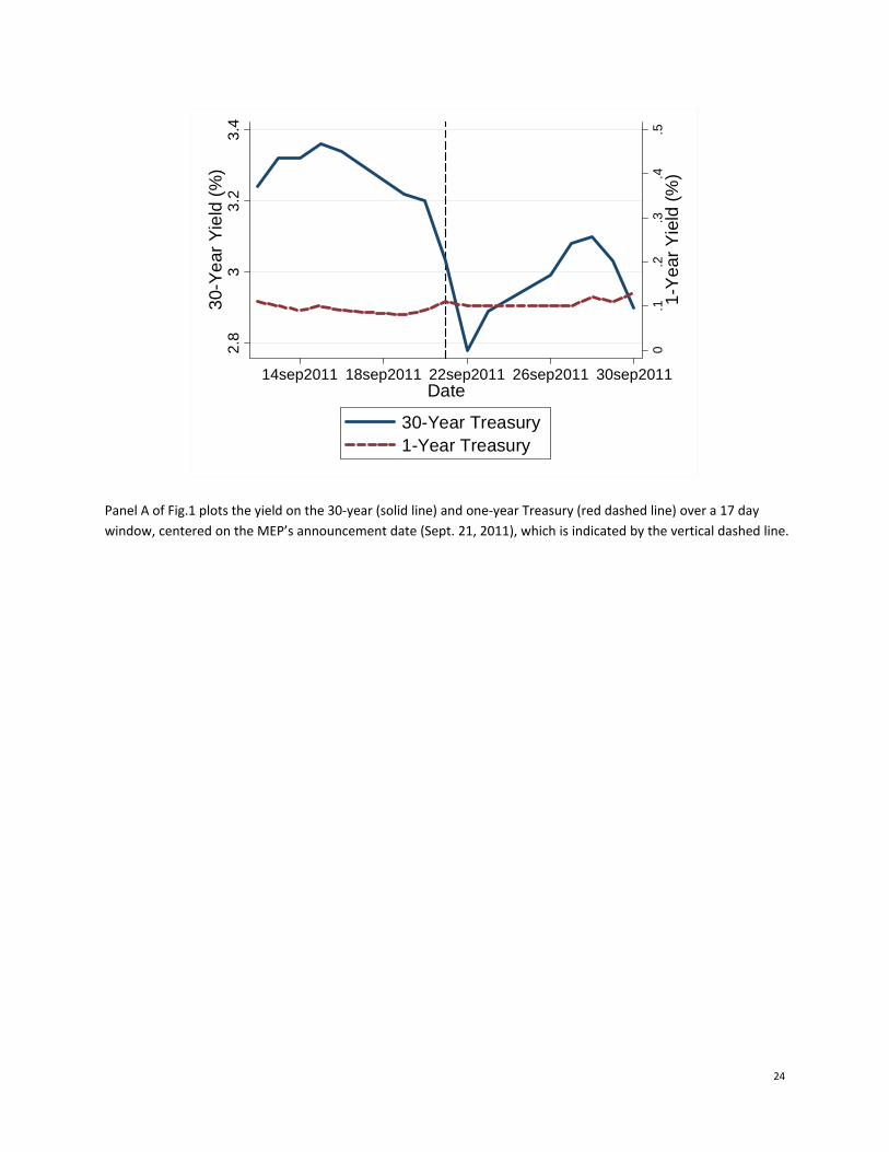
  24

 

Panel A of Fig.1 plots the yield on the 30‐year (solid line) and one‐year Treasury (red dashed line) over a 17 day 

window, centered on the MEP’s announcement date (Sept. 21, 2011), which is indicated by the vertical dashed line. 

 

 

 0

.1.2

.3.4

.51

-Yea

r Y

ield

(%

)

2.8

33

.23.

43

0-Y

ear

Yie

ld (

%)

14sep2011 18sep2011 22sep2011 26sep2011 30sep2011Date

30-Year Treasury1-Year Treasury

  25

 

Panel B of Fig.1 plots the cumulative change in the 30‐year Treasury yield at 30‐minute intervals over Sept. 21 and 

22, 2011. The vertical dashed line indicates the announcement time of the MEP at 2:23 p.m. on Sept. 21, 2011. The 

solid vertical line indicates the stock market opening time of Sept. 22, 2011. 

 

 

-.4

-.3

-.2

-.1

0C

um

ula

tive

Yie

ld C

han

ges

Sep21 9:30am

Sep21 10:30am

Sep21 11:30am

Sep21 12:30pm

Sep21 1:30pm

Sep21 2:30pm

Sep21 3:30pm

Sep22 9:30am

Sep22 10:30am

Sep22 11:30am

Sep22 12:30pm

Sep22 1:30pm

Sep22 2:30pm

Sep22 3:30pm

Treasury Yield Changes Zero

Intraday Long-Term Treasury Yield Changes

01

23

Yie

ld (

%)

0 10 20 30Maturity

Sep 20, 2011 Sep 21, 2011Sep 22, 2011

  26

Panel C of Fig. 1 plots the Treasury yield curve over a three-day window centered on Sept. 21, 2011.

 

Fig. 2 plots thday window column 8 of column 8 of T

he long-term debt around Sept. 22, Table 3, which re

Table 3. Standard e

Figure

dependence point2011, event date,

egresses abnormalerrors are clustered

2. Coefficient estim

t estimates and con, which is indicatel returns for a gived at the three-digit

mates around the ev

nfidence bands obted by the verticalen day on long-tet SIC level.

vent date

tained from a seril line. The regresserm debt dependen

es of daily regresssion specificationsnce and the set of

sions, for a 10-s are based on f controls from

27

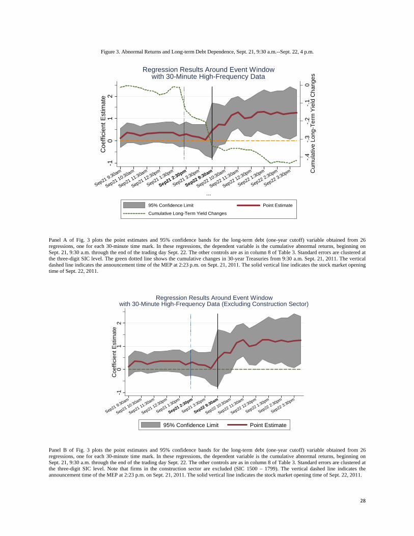
  28

Figure 3. Abnormal Returns and Long-term Debt Dependence, Sept. 21, 9:30 a.m.--Sept. 22, 4 p.m.

   

Panel A of Fig. 3 plots the point estimates and 95% confidence bands for the long-term debt (one-year cutoff) variable obtained from 26 regressions, one for each 30-minute time mark. In these regressions, the dependent variable is the cumulative abnormal returns, beginning on Sept. 21, 9:30 a.m. through the end of the trading day Sept. 22. The other controls are as in column 8 of Table 3. Standard errors are clustered at the three-digit SIC level. The green dotted line shows the cumulative changes in 30-year Treasuries from 9:30 a.m. Sept. 21, 2011. The vertical dashed line indicates the announcement time of the MEP at 2:23 p.m. on Sept. 21, 2011. The solid vertical line indicates the stock market opening time of Sept. 22, 2011.

 

Panel B of Fig. 3 plots the point estimates and 95% confidence bands for the long-term debt (one-year cutoff) variable obtained from 26 regressions, one for each 30-minute time mark. In these regressions, the dependent variable is the cumulative abnormal returns, beginning on Sept. 21, 9:30 a.m. through the end of the trading day Sept. 22. The other controls are as in column 8 of Table 3. Standard errors are clustered at the three-digit SIC level. Note that firms in the construction sector are excluded (SIC 1500 – 1799). The vertical dashed line indicates the announcement time of the MEP at 2:23 p.m. on Sept. 21, 2011. The solid vertical line indicates the stock market opening time of Sept. 22, 2011.

-.4

-.3

-.2

-.1

0C

umu

lativ

e Lo

ng-T

erm

Yie

ld C

han

ges

-10

12

Co

effic

ient

Est

ima

te

Sep21 9:30am

Sep21 10:30am

Sep21 11:30am

Sep21 12:30pm

Sep21 1:30pm

Sep21 2:30pm

Sep21 3:30pm

Sep22 9:30am

Sep22 10:30am

Sep22 11:30am

Sep22 12:30pm

Sep22 1:30pm

Sep22 2:30pm

Sep22 3:30pm

...

95% Confidence Limit Point Estimate

Cumulative Long-Term Yield Changes

Regression Results Around Event Windowwith 30-Minute High-Frequency Data

-10

12

Co

effic

ient

Est

ima

te

Sep21 9:30am

Sep21 10:30am

Sep21 11:30am

Sep21 12:30pm

Sep21 1:30pm

Sep21 2:30pm

Sep21 3:30pm

Sep22 9:30am

Sep22 10:30am

Sep22 11:30am

Sep22 12:30pm

Sep22 1:30pm

Sep22 2:30pm

Sep22 3:30pm

95% Confidence Limit Point Estimate

Regression Results Around Event Windowwith 30-Minute High-Frequency Data (Excluding Construction Sector)

  29

 

Panel C of Fig. 3 plots the point estimates and 95% confidence bands for the long-term debt (three-year cutoff) variable obtained from 26 regressions, one for each 30-minute time mark. In these regressions, the dependent variable is the cumulative abnormal returns, beginning on Sept. 21, 9:30 a.m. through the end of the trading day Sept. 22. The other controls are as in column 8 of Table 3. Standard errors are clustered at the three-digit SIC level. Note that these regressions use the full available sample of firms. The vertical dashed line indicates the announcement time of the MEP at 2:23 p.m. on Sept. 21, 2011. The solid vertical line indicates the stock market opening time of Sept. 22, 2011.

 

   

-10

12

Co

effic

ient

Est

ima

te

Sep21 9:30am

Sep21 10:30am

Sep21 11:30am

Sep21 12:30pm

Sep21 1:30pm

Sep21 2:30pm

Sep21 3:30pm

Sep22 9:30am

Sep22 10:30am

Sep22 11:30am

Sep22 12:30pm

Sep22 1:30pm

Sep22 2:30pm

Sep22 3:30pm

95% Confidence Limit Point Estimate

Regression Results Around Event Windowwith 30-Minute High-Frequency Data

(Long-term Debts with Three-Year Cutoff)

  30

Figure 4. Insurers’ Median Fixed Income Holdings Rated A- as a Share of Total NAIC Risk Category 1.

 

Fig. 4 plots the quarterly median holdings of fixed income securities rated A‐ as a share of the total NAIC risk category 1 (ratings AAA to A‐) from 

2002Q1 to 2013Q4.  The source for these data is Thompson Reuters’ eMAXX database of institutional bond holdings.  The shaded MEP region 

covers 2011Q4 through 2012Q4. 

 

 

   

MEP

.05.1

.15

2002q1 2005q1 2008q1 2011q1 2014q1

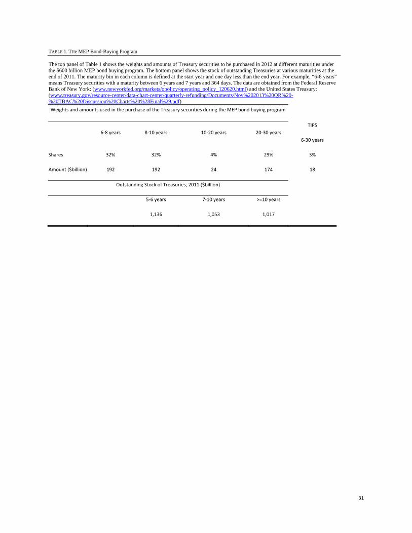
  31

TABLE 1. THe MEP Bond-Buying Program

The top panel of Table 1 shows the weights and amounts of Treasury securities to be purchased in 2012 at different maturities under the $600 billion MEP bond buying program. The bottom panel shows the stock of outstanding Treasuries at various maturities at the end of 2011. The maturity bin in each column is defined at the start year and one day less than the end year. For example, “6-8 years” means Treasury securities with a maturity between 6 years and 7 years and 364 days. The data are obtained from the Federal Reserve Bank of New York: (www.newyorkfed.org/markets/opolicy/operating_policy_120620.html) and the United States Treasury: (www.treasury.gov/resource-center/data-chart-center/quarterly-refunding/Documents/Nov%202013%20QR%20-%20TBAC%20Discussion%20Charts%20%28Final%29.pdf)

Weights and amounts used in the purchase of the Treasury securities during the MEP bond buying program

6‐8 years  8‐10 years  10‐20 years  20‐30 years 

TIPS 

6‐30 years 

Shares  32%  32%  4% 29% 3% 

Amount ($billion)  192  192  24 174 18 

Outstanding Stock of Treasuries, 2011 ($billion)

   5‐6 years 7‐10 years >=10 years   

      1,136  1,053 1,017   

   

  32

Table 2. Summary Statistics

Panel A of Table 2 reports the number of observations, mean, standard deviation, and various percentiles of two measures of long-term debt dependence and the key control variables. All variables are averages of firm-level characteristics through 2006. Variables are winsorized at the 1% level to reduce the effects of outliers. The data description in the appendix provides more detail on the variable constructions.

Variables  No. Obs.  MEAN SD 5% 25% 50%  75% 95%

Long‐Term Debt Dependence 

(One‐Year Cutoff) 3297  0.82  0.25  0.22  0.74  0.92  1.00  1.00 

Long‐Term Debt Dependence 

(Three‐Year Cutoff) 2713  0.43  0.3  0  0.15  0.45  0.67  0.9 

Market Capitalization (billions)  2564  1.58 4.24 0.02 0.11 0.35  1.09 6.49

Book‐to‐Market Ratio  2563  0.56 0.39 0.11 0.29 0.49  0.75 1.24

Total Debts (Normalized by Total 

Assets) 2713  0.36  0.96  0.000  0.003  0.03  0.22  2.00 

Total Assets  2717  1.16 2.85 0.01 0.05 0.22  0.80 5.79

Net Income Growth  2601  0.19 0.35 ‐0.32 0.06 0.14  0.30 0.81

Return on Assets  2447  0.00 0.09 ‐0.18 ‐0.017  0.03  0.05 0.07

Income over Assets  2634  ‐0.03 0.79 ‐0.85 0.06 0.15  0.21 0.37

Average Q  2542  6.33 16.09 1.18 1.58 2.43  4.81 18.05

Short‐Term Financial Constraint  2668  ‐0.13 1.16 ‐0.42 0.00 0.07  0.13 0.24

Capital Intensity  2634  0.06 0.05 0.02 0.03 0.05  0.07 0.14

 

 

 

 

   

  33

Panel B. Long-Term Debt Dependence (Ratio of Debt with Maturity Beyond One Year to Total Debt)

Panel B of Table 2 investigates the relationship between long-term debt dependence and other firm characteristics; all variables are averaged through 2006, creating a cross-section. In column 1, the dependent variable in the regression is long-term debt dependence; the regression also includes sector fixed effects (three-digit SIC code), and standard errors (in parentheses) are clustered at the sector level. Column 2 reports the simple bivariate correlation between long-term debt dependence and each variable. *** p<0.01, ** p<0.05, * p<0.1.

  (1)  (2)

OLS  Unconditional correlations

Market Capitalization (billions) 

‐0.0020  0.02

(0.0035) 

 

Book‐to‐Market Ratio 

‐0.014  ‐0.01

(0.013) 

 

Total Debt (Normalized by 

Total Assets) 

0.030**  0.10**

(0.013) 

 

Total Assets 

‐0.0057  0.07***

(0.0077) 

 

Net Income Growth 

0.011  ‐0.02

(0.018) 

 

Return on Assets 

‐0.0042  0.07**

(0.11) 

 

Income over Assets 

0.025*  0.12***

(0.013) 

 

Average Q 

‐0.0011**  ‐0.17***

(0.00049) 

 

Short‐Term Financial Constraint 

0.00091  0.01

(0.0040) 

 

Capital Intensity 

0.37**  0.03

(0.16) 

  34

Observations  2373 

 

R‐Squared  0.233 

 

Table 3. Stock Returns and MEP

This table reports regression results from an event study using daily stock returns. The dependent variable is abnormal stock returns on September 22, 2011, after controlling for the S&P 500 returns. Standard errors in parentheses are clustered at the SIC 3 industry level. *** p<0.01, ** p<0.05, * p<0.1. All columns except for column 1 includes sector fixed effects. In columns 1-8, long-term debt dependence is defined as the ratio of debt with a maturity in excess of one year divided by total debt; in column 9 this variable is computed using debt with a maturity in excess of three years in the numerator. In all columns except column 7, the variables are averaged before 2007. Column 7 computes these averages based on the last available data before September, 21 2011.

  (1)  (2)  (3) (4) (5) (6) (7)  (8)  (9)

Long‐Term Debt Dependence (One‐Year Cutoff) 

0.85**  0.91**  0.90** 0.93*** 0.97** 0.96** 1.61***  1.05***

0.39)  (0.43)  (0.36) 0.36) 0.38) 0.38) 0.50)  0.37)

Long‐Term Debt Dependence (Three‐Year Cutoff) 

0.24

0.32)

Market Capitalization (billions)  ‐0.0095 0.0079 0.0028 0.0048 ‐0.024  0.0053 0.0069

0.015) 0.015) 0.020) 0.0080) 0.023)  0.021) 0.022)

Book‐to‐Market Ratio   ‐0.62***  ‐0.60*** ‐0.55*** ‐0.37 ‐0.73***  ‐0.45* ‐0.49**

0.19) 0.19) 0.20) 0.35) 0.17)  0.23) 0.24)

Total Debt (Normalized by Total Assets) 

‐0.14 ‐0.15 ‐0.024 ‐0.11  ‐0.17  ‐0.16

0.086) 0.13) 0.055) 0.11)  0.13) 0.13)

Total Assets  0.012 ‐0.0078 0.027  0.012  0.00030

0.061) 0.020) 0.053)  0.064) 0.067)

Net Income Growth  ‐0.35 ‐0.012 0.014  ‐0.36  ‐0.37

0.25) 0.12) 0.36)  0.26) 0.27)

Return on Assets  1.92 3.28 0.23  1.62  1.78

1.64) 2.00) 1.07)  1.66) 1.69)

Income over Assets  ‐0.10 ‐0.52 0.16  ‐0.055 ‐0.093

0.13) 0.51) 0.19)  0.14) 0.13)

Average Q  0.018** ‐0.0038 0.019*  0.018** 0.016*

0.0074) 0.045) 0.012)  0.0077) 0.0085)

Short‐Term Financial Constraint  0.087 ‐0.37* 0.051  0.048  0.049

0.12) 0.21) 0.11)  0.11) 0.12)

Capital Intensity  ‐2.24 ‐2.64 ‐3.15  ‐1.88  ‐1.19

2.13) 3.63) 2.49)  2.19) 2.23)

Sensitivity to Monetary Shocks  43.6  33.1

62.7) 71.5)

Observations  2618  2618  2492 2492 2373 2373 2759  2344  2280

R‐Squared  0.003  0.145  0.150 0.150 0.154 0.151 0.155  0.147  0.148

 

   

  35

Table 4. Alternative Dates

This table reports regression results from a series of event studies using daily stock returns. Each event date is listed at the top of the column. Panel A focuses on the 10 days centered around September, 21st (the day of the MEP’s announcement), but for 2009, 2010 and 2012. Panel B focuses on the dates centered around QE2 and QE 3, as well as the MEP. In all cases, the dependent variable is abnormal stock returns after controlling for the S&P 500 returns. The independent variable of interest is long-term debt dependence: the ratio of debt with a maturity in excess of one year divided by total debt, and averaged through 2007. Each regression includes the same set of controls as in column 8 of Table 3. Standard errors in parentheses are clustered at the SIC 3 industry level. *** p<0.01, ** p<0.05, * p<0.1.

Panel A of Table 4. Event studies around same time of year

2009  Sep 14  Sep 15  Sep 16  Sep 17 Sep 18 Sep 21 Sep 22 Sep 23  Sep 24  Sep 25 Sep 28

  ‐0.94  ‐0.21  0.29  ‐0.13 0.68 ‐0.19 ‐0.77* ‐0.10  0.51  ‐0.61 0.28

  (0.61)  (0.51)  (0.45)  (0.46) (0.52) (0.49) (0.42) (0.42)  (0.44)  (0.37) (0.58)

           

2010  Sep 14  Sep 15  Sep 16  Sep 17 Sep 20 Sep 21 Sep 22 Sep 23  Sep 24  Sep 27 Sep 28

  0.100  ‐0.30  ‐0.31  0.55 0.28 ‐0.43 ‐0.31 0.29  0.11  ‐0.40 0.38

  (0.25)  (0.29)  (0.36)  (0.35) (0.57) (0.43) (0.42) (0.26)  (0.31)  (0.37) (0.29)

           

2012  Sep 14  Sep 17  Sep 18  Sep 19 Sep 20 Sep 21 Sep 24 Sep 25  Sep 26  Sep 27 Sep 28

  0.17  ‐0.62*  ‐0.55  ‐0.14 ‐0.091 ‐0.46 ‐0.31 ‐0.0095  ‐0.30  0.17 ‐0.080

   (0.38)  (0.33)  (0.50)  (0.38) (0.41) (0.43) (0.46) (0.29)  (0.30)  (0.35) (0.28)

           

 

Panel B of Table 4: Event studies  around announcement of different LSAPs  

QE2  Oct 27  Oct 28  Oct 29  Nov 1 Nov 2 Nov 3 Nov 4 Nov 5  Nov 8  Nov 9 Nov 10

2010  0.23  0.49  0.24  ‐0.47 0.50 0.035 ‐0.050 ‐0.34  ‐0.92** 0.18 0.25

  (0.42)  (0.36)  (0.39)  (0.40) (0.31) (0.40) (0.35) (0.54)  (0.42)  (0.34) (0.35)

           

MEP  Sep 14  Sep 15  Sep 16  Sep 19 Sep 20 Sep 21 Sep 22 Sep 23  Sep 26  Sep 27 Sep 28

2011  0.27  0.17  0.13  ‐0.63 ‐0.58 0.12 1.05*** 0.24  0.21  0.39 ‐0.53

  (0.29)  (0.29)  (0.41)  (0.43) (0.50) (0.40) (0.37) (0.33)  (0.27)  (0.33) (0.36)

           

QE3  Sep 6  Sep 7  Sep 10  Sep 11 Sep 12 Sep 13 Sep 14 Sep 17  Sep 18  Sep 19 Sep 20

2012  0.85*  ‐0.65*  ‐0.064  0.41 0.15 ‐0.83* 0.17 ‐0.62*  ‐0.55  ‐0.14 ‐0.089

   (0.48)  (0.35)  (0.42)  (0.37) (0.38) (0.47) (0.38) (0.33)  (0.50)  (0.38) (0.41)

 

 

 

   

  36

Table 5. The Change in Long-Term Debt and the MEP

Panel A. The dependent variable in column 1 is the growth in long-term debt outstanding (one year cutoff). In column 2, the dependent variable is the growth in short-term debt. Standard errors are clustered by firms and years. *** p<0.01, ** p<0.05, * p<0.1. The MEP indicator variable equals 1 if the year is 2012 and 0 otherwise. The sample period is 2007-2013, and all specifications include firm and year fixed effects, and all the time invariant firm observables in column 5 of Table 3 interacted with the MEP indicator variable. All time invariant variables are observed pre-2007. These variables also enter linearly as time varying controls. Variables are winsorized at the 1% level.    (1) (2) 

   Long‐Term Debt Growth Short‐Term Debt Growth 

Long‐Term Debt Dependence * MEP  0.33*** 0.34

(0.12) (0.25)

Market Capitalization (billions) * MEP  ‐0.0067 ‐0.0020

(0.0044) (0.019)

Book‐to‐Market Ratio * MEP  0.022 0.015

(0.015) (0.038)

Total Debt (Normalized by Total Assets) * MEP  0.018 0.024

(0.016) (0.068)

Total Assets * MEP  ‐0.0024 ‐0.011

(0.0053) (0.022)

Net Income Growth * MEP  0.12* 0.093

(0.072) (0.22)

Return on Assets * MEP  0.025 ‐0.61

(0.39) (0.81)

Income over Assets * MEP  0.028 0.091

(0.046) (0.13)

Average Q * MEP  ‐0.0033 0.0053

(0.0026) (0.0065)

Short‐Term Financial Constraint * MEP  0.0019 ‐0.0013

(0.031) (0.068)

Capital Intensity * MEP  0.36 0.050

(0.55) (1.70)

Number of Observations  16498 6129

R‐Squared 

 

 

 

  37

Table 5. The Change in Long-Term Debt and the MEP

Panel B: Financial Constraints. The dependent variable is the growth in long‐term debt outstanding (one year cutoff). In column 1, the sample is restricted to those firms that score below the 75th percentile of the age‐size index from Hadlock and Pierce (2010). Column 2 uses the sample of firms in the top quartile of this index. Higher values of the index suggest more financial constraints. The MEP indicator variable equals 1 if the year is 2012 and 0 otherwise. Column 3 uses the full sample of firms and includes Age‐Size Index interaction terms. The sample period is 2007‐‐2013. The control variables are identical to column 1 of Panel A.      (1)  (2) (3)

  Low  High Full Sample

Long‐Term Debt Dependence * MEP 

0.32***  0.25 0.31***

(0.12)  (0.25) (0.10)

Age‐Size Index* MEP      0.00010**

      (0.000048)

Age‐Size Index*Long‐Term Debt Dependence * MEP 

    ‐0.00014**

      (0.000057)

Number of Observations  12332  411216219 

 

 

 

 

 

 

 

 

 

 

 

 

   

  38

Table 6. Did a Firm Issue Debt?

Panel A. The dependent variable equals 1 if a firm issued debt in the calendar year and 0 otherwise. Standard errors clustered at the firm level for columns (1) and (2) and are clustered at firm and year levels for the other columns. *** p<0.01, ** p<0.05, * p<0.1. All specifications include year effects. Column 2 include a first-order autoregressive term. Column 3 includes firm fixed effects. Column 4 includes all the time invariant firm observables in column 5 of Table 3 interacted with the MEP indicator variable. The MEP indicator variable equals 1 if the year is 2012 and 0 otherwise. The sample period is 2007—2013. Iterations terms of MEP and average firm characteristics before 2007 are included in the regressions. In addition, time varying firm characteristics are included all regressions. These variables are Market capitalization, Book-to-Market Ratio, Total Debt, Long-term Debt, Total Assets, Net Income Growth, Return on Assets, Income over Assets, Average Q, Investment Opportunity, Short-term Financial Constraint, and Capital Intensity.

 

(1)  (2) (3) (4) 

Variables  No Controls  AR(1) Firm Fixed Effects Firm Controls

Long‐term Debt 

Dependence * MEP 

0.050***  0.049*** 0.045*** 0.040***

(0.0089)  (0.010) (0.0095) (0.015)

Observations  35771  29152 35771 21593 

R‐squared  0.013  0.163 0.469 0.502 

Panel B: Financial Constraints. The dependent variable equals 1 if a firm issued debt in the calendar year and 0 otherwise, and all regressions use the same controls as in column 4 of Panel A. In column 1, the sample is restricted to those firms that score below the 75th percentile of the age-size index from Hadlock and Pierce (2010). Column 2 uses the sample of firms in the top quartile of this index. Higher values of the index suggest more financial constraints. The MEP indicator variable equals 1 if the year is 2012 and 0 otherwise. Column 3 uses the full sample of firms and includes Age-Size Index interaction terms. The sample period is 2007--2013.   (1)  (2) (3)

  Low  High Full Sample

Long‐Term Debt Dependence * MEP 

0.050**  0.0049  0.040*** 

(0.022)  (0.0048)  (0.015) 

Age‐Size Index* MEP      ‐0.000034 

      (0.000024) 

Age‐Size Index*Long‐Term Debt Dependence * MEP 

   0.000040 

      (0.000028) 

Number of Observations 16039  5349  21104 

 

   

  39

Table 7. Reaching for Yield

Panel A: Bond Spreads. The dependent variable is the log spread between a bond and the corresponding Treasury of the same maturity. Numbers in parentheses are standard errors clustered at the issuer (firm) level. *** p<0.01, ** p<0.05, * p<0.1. All specifications include firm, year, and quarter fixed effects; the time-varying firm observables in Panel A Table 5; the log of the principal issued; log maturity; and the bond credit rating; these bond-level variables are also interacted with the MEP. All continuous variables are winsorized at the 1 percent level. Columns 2—5 also include the time-varying firm observables interacted with the MEP. Category 1 bonds are rated AAA through A-. Category 2 bonds are rated BBB+ through BBB-. The MEP indicator variable equals 1 if the year is 2012 and 0 otherwise. The sample period is 2007—2013.

   (1)  (2) (3) (4)  (5)

Variables  Category 1 Category 1 AAA to BBB+ Cats 1 & 2  Cats 1 & 2

        

A‐ Rating*MEP  ‐0.231** ‐0.295* ‐0.270***

(0.11) (0.17) (0.10)

BBB+ Rating*MEP  0.149

(0.14)

BBB‐ Rating*MEP  0.0961 

(0.13) 

        

Observations  738  738 994 1,590  1,590

R‐Squared  0.811 0.819 0.817 0.826  0.826

 

 

 

 

 

 

 

 

 

 

 

  40

 

 

 

 

 

 

Panel B: Insurer bond portfolios. The dependent variable in columns 1 and 2 is the share of A‐ debt in an insurer’s bond portfolio. In columns 3 and 4 the dependent variable is the share of A‐ debt in new bond purchases within the calendar year. “Pre‐crisis” variables are averaged over 2004‐2006. The data are a panel from 2007‐2013. All specifications include insurer and year fixed effects.  

    (1) (2) (3)  (4)

  A‐ share in portfolio A‐ share in new purchases

MEP * Pre‐crisis ratio of treasury to total earned income 

0.0725** 0.0603** 0.143**  0.159**

  (0.0278) (0.0289) (0.0642)  (0.0615)

Log of size of general account  0.0112 0.0113 ‐0.00529  ‐0.00430

  (0.00880) (0.00892) (0.0115)  (0.0115)

Portfolio duration weighted by amt held  ‐0.000206 ‐0.000350 0.00235  0.00226

  (0.00303) (0.00306) (0.00376)  (0.00373)

Squared portfolio duration weighted by amt held  7.27e‐05 7.70e‐05 ‐3.74e‐06  ‐2.95e‐06

  (8.39e‐05) (8.43e‐05) (0.000105)  (0.000104)

Portfolio rating weighted by amt held  1.430 1.072 ‐11.06  ‐8.223

  (6.017) (5.638) (9.493)  (7.692)

MEP * Log of size of general account  ‐0.00120 ‐0.00225 0.00176  ‐0.00447

  (0.00181) (0.00424) (0.00328)  (0.00800)

MEP * Portfolio duration weighted by amt held  0.00248 0.00608* ‐0.000561  ‐0.00497

  (0.00342) (0.00357) (0.00774)  (0.00917)

MEP * Squared portfolio duration weighted by amt held 

‐7.36e‐05 ‐0.000204 2.62e‐05  0.000206

  (0.000136) (0.000140) (0.000336)  (0.000370)

MEP * Portfolio rating weighted by amt held  ‐0.551 ‐2.108 14.58  12.81

  (3.723) (4.039) (14.22)  (9.457)

MEP * Pre‐crisis share of portfolio in A‐ rated securities 

0.0100 0.0407 0.0656  0.0624

  (0.0981) (0.108) (0.189)  (0.213)

MEP * Pre‐crisis log of size of general account  0.000396 0.0119

  (0.00440) (0.00827)

MEP * Pre_crisis portfolio duration weighted by amt held 

‐0.00769* 0.00419

  (0.00408) (0.00811)

MEP * Pre‐crisis squared portfolio duration weighted by amt held 

0.000295** ‐0.000202

  (0.000130) (0.000249)

MEP * Pre‐crisis portfolio rating weighted by amt held 

2.663 46.09

  (17.47) (30.58)

Observations  1,126 1,126 1,122  1,122

R‐squared  0.628 0.630 0.371  0.374

  41

 

 

 

Table 8. The Real Effects of the MEP

Panel A. The dependent variable in column 1 is the growth in plant and equipment expenditures (PPENT). In column 2, it is the growth in the number of employees; column 3 uses the growth in cash holdings and column 4 is the growth in dividend and share repurchases. Standard errors are clustered at the firm-year level. *** p<0.01, ** p<0.05, * p<0.1. The MEP indicator variable equals 1 if the year is 2012 and 0 otherwise. The sample period is 2007—2013. Time varying firm characteristics are included in all regressions. These variables are Market capitalization, Book-to-Market Ratio, Total Debt, Long-term Debt, Total Assets, Net Income Growth, Return on Assets, Income over Assets, Average Q, Investment Opportunity, Short-term Financial Constraint, and Capital Intensity. All regressions also include firm and year fixed effects.

(1) (2) (3)  (4)

   Growth in PPENT  Growth in Employees 

Growth in Cash 

Holdings 

Growth in Dividend and 

Share Repurchase 

Long‐term Debt Dependence * MEP  0.085** 0.057** 0.012  0.0081

(0.039) (0.025) (0.087)  (0.16)

Market Capitalization (billions) * MEP 

0.00018 ‐0.00066 ‐0.00082  ‐0.0020

(0.0016) (0.0013) (0.0049)  (0.0093)

Book to Market Ratio * MEP 

0.016* ‐0.00011 ‐0.024  0.0063

(0.0096) (0.0054) (0.020)  (0.030)

Total Debt (normalized by total assets) * 

MEP 

0.016** 0.014** 0.00022  ‐0.037

(0.0066) (0.0055) (0.018)  (0.037)

Total Assets * MEP 

‐0.0043* ‐0.0038** 0.0046  0.0023

(0.0023) (0.0018) (0.0063)  (0.011)

Net income growth * MEP 

0.020 0.011 0.10  0.051

(0.031) (0.018) (0.061)  (0.15)

Return on Assets * MEP 

‐0.22 0.072 ‐0.18  0.33

(0.15) (0.087) (0.32)  (0.70)

Income over assets * MEP 

0.020 ‐0.0098 ‐0.024  ‐0.037

(0.020) (0.014) (0.047)  (0.074)

Average Q * MEP 

‐0.000091 0.00030 ‐0.0011  ‐0.0024

(0.0011) (0.00072) (0.0023)  (0.0035)

  42

Short‐term Financial Constraint * MEP 

0.0090 ‐0.0061 ‐0.013  ‐0.011

(0.016) (0.0090) (0.024)  (0.046)

Capital Intensity * MEP 

‐0.059 ‐0.31** ‐0.76  ‐1.54**

(0.21) (0.14) (0.50)  (0.78)

     

Number of Observations   26128  24642   25814   13723 

 

Panel B: Alternative measure of long‐term debt dependence.  Panel B replicates Panel A but long‐term debt dependence is defined as the ratio of debt with remaining maturity in excess of three years divided by total debt. Standard errors are clustered at the firm‐year level. *** p<0.01, ** p<0.05, * p<0.1. The MEP indicator variable equals 1 if the year is 2012 and 0 otherwise. The sample period is 2007‐‐2013. As with Panel A, interaction terms between the MEP and firm characteristics observed before 2007 are included in the regressions. In addition, time varying firm characteristics are included all regressions. These variables are Market capitalization, Book‐to‐Market Ratio, Total Debt, Long‐term Debt, Total Assets, Net Income Growth, Return on Assets, Income over Assets, Average Q, Investment Opportunity, Short‐term Financial Constraint and Capital Intensity. 

   (1) (2) (3) (4)

 

Growth in PPENT  Growth in Employees  Growth in Cash Holdings Growth in Dividend and 

Share Repurchase 

Long‐term Debt Dependence (3Years) 

* MEP 

0.058** 0.058*** 0.15* ‐0.10

(0.026) (0.021) (0.080)  (0.13)

Number of Observations  25135 23740 24846  13216

 

Panel C: Financing constraints. The dependent variable in columns 1-3 is the growth in plant and equipment expenditures. In columns 4-6, the dependent variable is the growth in the number of employees. In columns 1 and 4, the sample is restricted to those firms that score below the 75th percentile of the age-size index from Hadlock and Pierce (2010). Columns 2 and 5 use the sample of firms in the top quartile of this index. Columns 3 and 6 use the full sample of firms and includes Age-Size Index interaction terms. Higher values of the index suggest more financial constraints. The MEP indicator variable equals 1 if the year is 2012 and 0 otherwise. The sample period is 2007--2013. The other variables are as in Panel A.   Growth in PPENT Growth in Employees 

  (1)  (2) (3) (4) (5)  (6)

  Low  High Full Sample Low High  Full Sample

Long‐Term Debt Dependence * MEP 

0.063***  0.020  0.070*  0.055  0.058  0.058** 

(0.024)  (0.057)  (0.042)  (0.035)  (0.100)  (0.025) 

Age‐Size Index* MEP      0.000033**  0.000016 

      (0.000014)  (0.000012) 

Age‐Size Index*Long‐Term Debt Dependence * MEP 

   ‐0.000036*  ‐0.000014 

      (0.000021)  (0.000019) 

 Number of Observations 

18427  6144  21333  19526  6513 

  20256 

  43

References 

Adrian, Tobias, Paolo Colla, and Hyun Shin. 2013. “Which Financial Frictions? Parsing the Evidence from 

the Financial Crisis of 2007—09 ,” NBER Macroeconomics Annual, Volume 27, Daron Acemoglu, 

Jonathan Parker, and Michael Woodford, editors, 159‐214. 

Adrian, Tobias, and Hyun Shin. 2010. "The Changing Nature of Financial Intermediation and the Financial 

Crisis of 2007–2009," Annual Review of Economics, 2(1), 603‐618. 

Badoer, Dominique C., and Christopher M. James. Forthcoming. "The Determinants of Long‐Term 

Corporate Debt Issuances," Journal of Finance 

Barclay, Michael j., and Clifford W. Smith Jr.1995. "The Maturity Structure of Corporate Debt," Journal of 

Finance, 50(2) 609‐631 

Bates, Thomas W., Kathleen M. Kahle, and René M. Stulz. 2009. "Why Does US Firms Hold So Much 

More Cash Than They Used to?" Journal of Finance 64(5) 

Bernanke, Ben S., and Kenneth N. Kuttner. 2005. "What Explains the Stock Market's Reaction to Federal 

Reserve Policy?" Journal of Finance, 60(3), 1221‐1257. 

Becker, Bo, and Victora Ivashina. Forthcoming. "Reaching for Yield in the Bond Market", Journal of 

Finance. 

Becker, Bo, and Victora Ivashina. 2014. "Cyclicality of Credit Supply: Firm Level Evidence," Journal of 

Monetary Economics, 62(C), 76‐93. 

Benmelech, Ephraim, Ralf Meisenzahl and Rodney Ramcharan. 2014. "The Real Effects of Liquidity 

During the Financial Crisis: Evidence from Automobiles", SSRN Working Paper 2511181. 

Berglof, Erik, and Ernst‐Ludwig Thadden. 1994. "Short‐Term Versus Long‐Term Interests: Capital 

Structure with Multiple Investors," Quarterly Journal of Economics, 109(4), 1055‐84. 

Bloom, Nicholas. 2009. "The Impact of Uncertainty Shocks," Econometrica, 77(3), 623‐685. 

Borio, Claudio, and Haibin Zhu. 2012. "Capital Regulation, Risk‐Taking and Monetary Policy: A Missing 

Link in the Transmission Mechanism?" Journal of Financial Stability, 8(4), 236‐251. 

Cahill, Michael E., Stefania D'Amico, Canlin Li, and Jonh S. Sears. 2013. "Duration Risk Versus Local 

Supply Channel in Treasury Yields: Evidence from the Federal Reserve's Asset Purchase 

Announcements,"  Finance and Economics Discussion Series, Board of Governors of the Federal 

Reserve System (U.S.). 

Chodorow‐Reich, Gabriel. 2014. "Effects of Unconventional Monetary Policy on Financial Institutions," 

Brookings Papers on Economic Activity, 48(1), 155‐227. 

Crouzet, Nicolas. 2014. "Firm Investment and the Composition of Debt", SSRN Working Paper 2524589. 

  44

Diamond, Douglas W. 1991. "Debt Maturity Structure and Liquidity Risk,"  Quarterly Journal of 

Economics, 106(3), 709‐37. 

DeAngelo, Harry, and Richard Roll. 2015. “How Stable Are Corporate Capital Structures?” Journal of 

Finance, 70(1) 373–418. 

De Fiore, Fiorella, and Harald Uhlig. 2015 "Corporate Debt Structure and the Financial Crisis" Journal of 

Money, Credit and Banking, 47(8) 1571‐1598 

DiMaggio, Marco, and Marcin Kacperczyk. 2015. "The Unintended Consequences of the Zero Lower 

Bound Policy", SSSRN Working Paper 2458587. 

DiMaggio, Marco, Amir Kermani, and Rodney Ramcharan. 2014. "Monetary Policy Pass Through: 

Household Consumption and Voluntary Deleveraging," SSRN Working Paper 2489793. 

Eggertsson, Gauti. B., and Michael Woodford. 2006. "Optimal Monetary and Fiscal Policy in a Liquidity 

Trap," In NBER International Seminar on Macroeconomics 2004, National Bureau of Economic 

Research, Inc., 75‐144. 

Ellul, Andrew, Chotibhak Jotkasthira, Christian Lundbald and Yihui Wang. "Is Historical Cost Accounting a 

Panacea? Market Stress, Incentive Distortions and Gains Trading", forthcoming Journal of 

Finance. 

Estrella, Arturo, and Gikas A. Hardouvelis. 1991. "The Term Structure as a Predictor of Real Economic 

Activity," Journal of Finance, 46(2), 555‐76. 

Farre‐Mensa, Joan, and Alexander Ljungqvist. 2015. “Do Measures of Financial Constraints Measure 

Financial Constraints?” SSRN Working Paper 2338575. 

Faulkender, Michael, and Mitchell A. Petersen. 2006. "Does the Source of Capital Affect Capital 

Structure?" Review of Financial Studies, 19(1), 45‐79. 

Fazzari, Steven M., R. Glenn Hubbard, and Bruce C. Petersen. 1988. “Financing Constraints and Coporate 

Investment," Brookings Papers on Economic Activity, 19(1), 141‐206 

Flannery, Mark J. 1986. "Asymmetric Information and Risky Debt Maturity Choice," Journal of Finance, 

41(1), 19‐37. 

Gagnon, Joseph, Matthew Raskin, Julie Remache, and Brian Sack. 2011. "Large‐scale asset purchases by 

the Federal Reserve: did they work?" Economic Policy Review (May), 41‐59. 

Gertler, Mark, and Peter Karadi. 2011. "A model of unconventional monetary policy," Journal of 

Monetary Economics, 58(1), 17‐34. 

Gertler, Mark, and Peter Karadi. 2013. "QE 1 vs. 2 vs. 3. . . : A Framework for Analyzing Large‐Scale Asset 

Purchases as a Monetary Policy Tool," International Journal of Central Banking, 9(1), 5‐53. 

  45

Gorodnichenko, Yuriy, and Michael Weber. 2013. "Are Sticky Prices Costly? Evidence From The Stock 

Market," NBER Working Papers, National Bureau of Economic Research, Inc. 

Greenwood, Robin, and Samuel G. Hanson. 2013. "Issuer Quality and Corporate Bond Returns," Review 

of Financial Studies, 26(6), 1483‐1525. 

Greenwood, Robin, Samuel G. Hanson, and Jeremy C. Stein, 2010. "A Gap‐Filling Theory of Corporate 

Debt Maturity Choice," Journal of Finance, 65(3), 993‐1028. 

Guedes, Jose, and Tim Opler. 1996. "The Determinants of the Maturity of Corporate Debt Issues," 

Journal of Finance, 51(5), 1809‐1833. 

Guerrieri, Veronica, and Péter Kondor. 2012. "Fund Managers, Career Concerns, and Asset Price 

Volatility," American Economic Review, 102(5), 1986‐2017. 

Gürkaynak, Refet S., Brian Sack, and Eric Swanson. 2005." Do Actions Speak Louder Than Words? The 

Response of Asset Prices to Monetary Policy Actions and Statements," International Journal of 

Central Banking, 1(1). 

Hamilton, James D., and Jing Cynthia Wu. 2012. "The Effectiveness of Alternative Monetary Policy Tools 

in a Zero Lower Bound Environment,", Journal of Money, Credit and Banking, 44(2), 3‐46. 

Hanson, Samuel G., and Jeremy C. Stein. Forthcoming. "Monetary policy and long‐term real rates," 

Journal of Financial Economics. 

Hart, Oliver, and John Moore. 1994. "A Theory of Debt Based on the Inalienability of Human Capital," 

Quarterly Journal of Economics, 109(4), 841‐79. 

Hoshi, Takeo, Anil Kashyap, and David Scharfstein. 1991. "Coporate Structure, Liquidity, and Investment 

Evidence from Japanese Industrial Groups," Quarterly Journal of Economics, 106(1), 33‐60. 

Huang, Xin, Hao Zhou, and Haibin Zhu. 2009. "A Framework for Assessing the Systemic Risk of Major 

Financial Institutions," Journal of Banking and Finance, 33(11) 2036‐2049. 

Hubbard, R. Glenn, Anil Kashyap, and Toni Whited. 1995. "International Finance and Firm Investment," 

Journal of Money, Credit and Banking, 27(3), 683‐701. 

Kaplan, Steven N., and Luigi Zingales. 1997. "Do Investment‐Cash Flow Sensitivities Provide Useful 

Measures of Financing Constraints,"  Quarterly Journal of Economics, 112(1), 169‐215. 

Keys, Benjamin J., Tomasz Piskorski, Amit Seru, and Vincent Yao. 2014. "Mortgage Rates, Household 

Balance Sheets, and the Real Economy," NBER Working Paper 20561. 

King, Mervyn. 2013. “Monetary Policy: Many Targets, Many Instruments. Where do We Stand?” remarks 

given by the Governor of the Bank of England at the IMF Conference on Rethinking Macro Policy 

II: First Steps and Early Lessons.  

  46

Krishnamurthy, Arvind, and Annette Vissing‐Jorgensen. 2011. "The Effects of Quantitative Easing on 

Interest Rates: Channels and Implications for Policy," Brookings Papers on Economic Activity, 

43(2 (Fall)), 215‐287. 

Krishnamurthy, Arvind, and Annette Vissing‐Jorgensen. 2013. "The Ins and Outs of LSAPs" Proceedings. 

Kuttner, Kenneth N. 2001. "Monetary policy surprises and interest rates: Evidence from the Fed funds 

futures market," Journal of Monetary Economics, 47(3), 523‐544. 

MacKinlay, A. Craig. 1997. "Event Studies in Economics and Finance," Journal of Economic Literature, 

35(1), 13‐39. 

Merril, Craig, Taylor Nadauld and Phillip Strahan. 2014. "Final Demand for Structured Finance Securities", 

Unpublished Working paper. 

Myers, Stewart C. 1977. "Determinants of Corporate Borrowing," Journal of Financial Economics, 5(2), 

147‐175. 

Morris, Stephen, and Hyun Song Shin. 2012. "Contagious Adverse Selection," American Economic Journal: 

Macroeconomics, 4(1), 1‐21. 

NAIC. 2014. "New Issuance of Corporate Bonds and U.S. Insurer Corporate Bond Portfolios," Capital 

Markets Special Report 3/7/14. 

Ramcharan, Rodney, Skander Van den Heuvel, and Stephane Verani. Forthcoming. "From Wall Street to 

Main Street: the Impact of the Financial Crisis on Consumer Credit Supply," Journal of Finance. 

Rajan, Raghuram. 2013. "A Step in the Dark: Unconvential Monetary Policy After the Crisis," Andrew 

Crockett Memoral Lecture. 

Rauh, Joshua D., and Amir Sufi. 2010. "Capital Structure and Debt Structure," Review of Financial Studies, 

23(12), 4242‐4280. 

Shleifer, Andrei, and Robert Vishny. 2011. "Fire Sales in Finance and Macroeconomics," Journal of 

Economic Perspectives, 25(1), 29‐48. 

Stein, Jeremy C. 2013. "Yield‐Oriented Investors and the Monetary Transmission Mechanism," Speech at 

the Banking, Liquidity and Monetary Policy Symposium, Center for Financial Studies, Frankfurt, 

Germany, September 26, 2013. 

Stein, Jeremy C. 2014. "Incorporating Financial Stability Considerations into a Monetary Policy 

Framework," Speech at the International Research Forum on Monetary Policy, Washington, D.C., 

March 21, 2014. 

Swanson, Eric T., and John C. Williams. Forthcoming. "Measuring the Effect of the Zero Lower Bound on 

Yields and Exchange Rates," American Economic Review. 

  47

Vayanos, Dimitri, and Jean‐Luc Vila. 2009. "A Preferred‐Habitat Model of the Term Structure of Interest 

Rates." Working Paper, National Bureau of Economic Research. 

Wheelock, David C., and Mark E. Wohar. 2009. "Can the Term Spread Predict Output Growth and 

Recessions? a Survey of the Literature," Review, (Sep), 419‐440. 

Whited, Toni M., and Guojun Wu. 2006. "Financial Constraints Risk," Review of Financial Studies, 19(2), 

531‐559. 

Wright, Jonathan H. 2012. "What does Monetary Policy do to Long‐Term Interest Rates at the Zero 

Lower Bound?", Economic Journal, 122(564), F447‐‐F466. 

 

Appendix: Data Description 

The firm level data come from Compustat. Variables of firms’ financial statement variables are 

downloaded for U.S. firms at an annual frequency for all years that are available. Financial firms with SIC 

code between 6000 and 6999 are dropped.  

 

Long‐Term Debt Dependence 

We construct the baseline long‐term debt dependence as follows: in financial statements, assets 

and liabilities of different maturities are distinguished at the one‐year cutoff. Following Greenwood, 

Hanson, and Stein (2010), long‐term liability is defined as all debts with a maturity of one year or longer. 

Since some of the short‐term liabilities on the balance sheets are long‐term debts with remaining 

maturing less than one year, the total amount of long‐term debts is the sum of total long‐term debt (dltt) 

and long‐term debt due in one year (dd1). Similarly, short‐term debt is calculated as Debt in Current 

Liabilities minus long‐term debt due in one year (dd1). This ratio is then averaged over years to obtain 

the long‐term debt dependence ratio. For the baseline case, the average is computed with observations 

before 2007.  

We compute long‐term debt dependence with maturity in excess of three years as follows. The 

variables dd2 and dd3 measure debt with remaining maturity between one and two years, and two and 

three years, respectively. Total long‐term debt (dltt)‐dd2‐dd3 gives the stock of debt with maturity in 

excess of three years. Unfortunately, because variables like dd2 and dd3 measure the remaining 

maturity of debt, rather than the maturity at issuance, a long‐term loan (at issuance) can be 

misclassified as a short‐term loan if the long‐term loan is close to maturity. 20 Consider a loan that was 

issued with maturity of 30 years and is now 28 years old. This loan will have a remaining maturity of two 

                                                            

20 The choice of remaining maturity and issuance maturity does not affect long‐term debts measures with one‐

year cutoff. The two measures are identical for the one‐year cutoff. 

  48

years (dd2), and be omitted in an imputation like ddlt‐dd2‐dd3, potentially mismeasuring a firm’s long‐

term debt dependence. This mismeasurement problem can become worse when the imputation is 

extended to longer maturities dd4 and dd5. 

Also, the reporting in Compustat can make these imputations unreliable. In the case of dltt‐dd2‐

dd3, some 3.5% of the observations are negative, and another 32% are missing, relative to the baseline 

one year cutoff definition for long‐term debt. Extending the imputation to debt with remaining maturity 

beyond five years: dltt‐dd2‐dd3‐dd4‐dd5 gives negative values in 9.1% of the observations, and missing 

values in 37% of the cases relative to the one year cutoff baseline. 

 

Other Controls 

A couple of size variables are controlled for in the model. All variables are at an annual 

frequency. Total assets are obtained directly from Compustat (at). Market capitalization is the product 

of closing stock price on financial year end (prcc_f) and total amount of outstanding common shares of 

the firm (csho). Sizes of debts are controlled for by total long‐term debts and total debts, both 

normalized by lagged total assets (at). Book‐to‐market ratio is the ratio of book equity (ceq) over market 

capitalization.  We have a few measures of firms' profitability: (1) net income growth is the log growth 

rate of firms net income (item ni); (2) return on assets is net income divided by the sum of market 

capitalization and total liabilities (item ni divided by the sum of market capitalization and lt); (3) i2a is 

computed by dividing operating income before depreciation (item oibdp) normalized by lagged total 

assets. 

Two measures are used to control for firms' investment opportunity: average Q and investment 

opportunity i2s. A firm's average Q is the sum of market capitalization and total assets minus book 

equity and all normalized by lagged total assets. Investment opportunity is defined to be capital 

expenditure (item capx) divided by net sales (item sale) of firms. This variable is similarly defined as in 

Gorodnichenko and Weber (2013). Capital intensity (d2a) is the ratio of depreciation (dp) over lagged 

total assets (at). 

We have variables to measure a firm's dependence on short term financing and external 

financing and. Short‐term financing need (rp2s) is calculated first by taking the difference between 

receivables (rect) and payables (ap), and then by the dividing this difference by total sales (sale).  

And as before, to limit any spurious associations induced by the crisis, we take the historical 

average of all the control variables through 2007. For robustness, we also try taking the average of the 

control variables through to Sept. 21, 2011, or just use the last available observation before 2007. All 

variables are winsorized at the 1% level to reduce the impact of outliers. 

In the sections of evaluating the effect of MEP on firm activities, we have other firm‐level 

variables at an annual frequency. Growth in long‐term debts and in short‐term debts are log growth 

rates of long‐term debts and short‐term debts, respectively. Growth in properties, plants, and 

  49

equipment, a measure of net investment, is computed as the log growth rate of the item ppent in 

Compustat.  Growth in employment is computed as the log growth rate of the item emp in Compustat. 

Similarly, growth in cash holdings is the log growth rate of cash and short‐term investments (item che) in 

Compustat. Dividend and shares repurchase is equal to total dividend (item dvt) plus purchase of 

preferred and common stocks (item prstkc) minus redemption of preferred stocks (item pstkrv). Then 

we compute the log growth rate for this variable. All of these four variables are winsorized at the 1% 

level. 

 

Abnormal Returns 

We obtained daily returns of stocks of public firms from CRSP to compute abnormal returns. The 

abnormal returns used on the left hand side of the regressions are predicted residuals from a one‐factor 

model controlling for market returns (MacKinlay, 1997). To be more specific, suppose the event date is 

denoted as T, we first run a one‐factor regression using data range from one year and one month before 

the event date to one month before the event date. The one‐factor regression for firm i is given as 

 

 

 

where t=T‐395,...,T‐30, and   the returns of the S&P 500 portfolio. After obtaining the 

coefficient estimates   and  , the abnormal returns are computed as the predicted residuals   ̂

 for firm i at event date T. 

 

Bond Data 

We obtain bond issuance data from the Mergent FISD database, which contains comprehensive 

bond issuance data since the 1980s. The database provides a lot of information about a particular 

issuance, including date of issuance, maturity, amount issued, coupon, and credit rating. We first 

collected all bond issuances for nonfinancial firms from FISD. From the data, we see that a firm typically 

issues very few bonds per year. For example, among firms that have ever issued a corporate bond in a 

given year, over 50% of those firm issued only one corporate bond in that year. Given this sparse nature 

of bond issuance, we aggregate the issuance to firm‐calendar year and merge the data set from FISD to 

the Compustat file by CUSIP and company names. This merge results in a match of 2,517 firm year, and 

it allows us to test whether the MEP affected the probability of a firm issuing a corporate bond.   

We constructed NAIC bond credit ratings from the credit ratings assigned by the three major 

credit rating agencies and provided by FISD.  Following the NAIC procedure similarly applied by Becker 

  50

and Ivashina (forthcoming), we compute the median credit rating when all three ratings are available, 

and the minimum credit rating when only two ratings are available.  

 

Insurance company data 

Our source for information about insurance companies is the annual statutory filings collated by 

the National Association of Insurance Commissioners and provided by SNL Financial.  We extract data on 

individual bond holdings from the Schedule D (Part 1), including bond identifier (CUSIP), type of bond 

(e.g. Treasury), the date of first purchase, the residual maturity, and the par value held. We obtain the 

size of each insurer company’s portfolio, excluding the separate account, from the summary balance 

sheet tables.  And we collect data on the income earned from Treasuries from the exhibit of net 

investment income.  We merge these data with the FISD database to obtain ratings information for each 

bond at year end.  Our final sample is an unbalanced panel of 150 insurance companies over the years 

2004‐2014.