IZA DP No. 3380

The Impact of Unilateral Divorce on Crime

Julio Cáceres-DelpianoEugenio Giolito

DI

SC

US

SI

ON

PA

PE

R S

ER

IE

S

Forschungsinstitutzur Zukunft der ArbeitInstitute for the Studyof Labor

March 2008

The Impact of Unilateral Divorce on Crime

Julio Cáceres-Delpiano Universidad Carlos III de Madrid

Eugenio Giolito

Universidad Carlos III de Madrid and IZA

Discussion Paper No. 3380 March 2008

IZA

P.O. Box 7240 53072 Bonn

Germany

Phone: +49-228-3894-0 Fax: +49-228-3894-180

E-mail: iza@iza.org

Any opinions expressed here are those of the author(s) and not those of IZA. Research published in this series may include views on policy, but the institute itself takes no institutional policy positions. The Institute for the Study of Labor (IZA) in Bonn is a local and virtual international research center and a place of communication between science, politics and business. IZA is an independent nonprofit organization supported by Deutsche Post World Net. The center is associated with the University of Bonn and offers a stimulating research environment through its international network, workshops and conferences, data service, project support, research visits and doctoral program. IZA engages in (i) original and internationally competitive research in all fields of labor economics, (ii) development of policy concepts, and (iii) dissemination of research results and concepts to the interested public. IZA Discussion Papers often represent preliminary work and are circulated to encourage discussion. Citation of such a paper should account for its provisional character. A revised version may be available directly from the author.

IZA Discussion Paper No. 3380 March 2008

ABSTRACT

The Impact of Unilateral Divorce on Crime*

In this paper, we evaluate the impact of unilateral divorce on crime. First, using crime rates from the FBI’s Uniform Crime Report program for the period 1965-1998 and differences in the timing in the introduction of the reform, we find that unilateral divorce has a positive impact on violent crime rates, with an 8% to 12% average increase for the period under consideration. Second, arrest data not only confirms the findings of a positive impact on violent crime but also shows that this impact is concentrated among those age groups (15 to 24) that are more likely to engage in these type of offenses. Specifically, for the age group 15-19, we observe an average impact over the period under analysis of 40% and 36% for murder and aggravated assault arrest rates, respectively. Disaggregating total arrest rates by race, we find that the effects are driven by the Black sub-sample. Third, using the age at the time of the divorce law reform as a second source of variation to analyze age-specific arrest rates we confirm the positive impact on the different types of violent crime as well as a positive impact for property crime rates, controlling for all confounding factors that may operate at the state-year, state age or age-year level. The results for murder arrests and for homicide rates (Supplemental Homicide Report) for the 15-24 age groups are robust with respect to specifications and specifically those that include year-state and year-age dummies. The magnitude goes from 15% to 40% depending on the specification and the age at the time of the reform. JEL Classification: J12, J13 Keywords: unilateral divorce, crime rates, arrest rates Corresponding author: Eugenio Giolito Department of Economics Universidad Carlos III de Madrid C/Madrid, 126 Getafe (Madrid) 28903 Spain E-mail: egiolito@eco.uc3m.es

* We thank Dan Black, Antonio Cabrales, Nezih Guner and Seth Sanders for their helpful comments. Financial support from the Spanish Ministry of Education, Grant BEC2006-05710, and from the European Commission (MRTN-CT-2003-50496) are gratefully acknowledged. Errors are ours.

2

1. Introduction

Family as institution has undergone a “complete make-over” in the U.S. and in the Western Hemisphere

during the last fifty years. Institutional and technological changes such as abortion and contraceptive methods

have not only changed the gender roles (Goldin and Katz, 2002) but also the family backgrounds faced by the

new generations. Children as never before are as likely to growth up in a one parent or a blended family, or

with a working mother. Among the most important institutional changes was the reform in divorce legislation

to the extent that it has been called the “Divorce Revolution”. Specifically, unilateral divorce, the right of one

spouse to ask for a divorce without the consent of the other, is the aspect of the reform that has captured the

greatest attention in the literature during the last twenty years.1

Initially, the scholarly debate was focused on the impact of unilateral divorce on divorce rates (Peters, 1986;

Friedberg, 1998; Gruber, 2004). Nowadays, there is growing consensus in the literature regarding a short-term

increase in divorce rates (Wolfers, 2006). This evidence has been related by scholars to a greater selection

into and out of marriage in adopting states, and therefore to an increase in the average match-quality of new

and surviving marriages.2 Despite the direct effects of unilateral divorce on divorce rates, recent research has

focused on the role of the reform in several other aspects of individual behavior. Some examples are studies

on family formation (Drewianka, 2004; Rasul, 2004; Alesina and Giuliano, 2007), marriage-specific

investments (Stevenson 2007) or female labor supply (Gray, 1998; Chiappori, Fortin and Lacroix, 2002;

Stevenson 2007b). The evidence in these studies also points towards a change in behavior in those couples

formed under the new legislation.

Stevenson and Wolfers (2006) provide a link between unilateral divorce and crime. Specifically, they

consider two types of offenses: domestic violence and homicide committed by a spouse3. They show that in

states that introduced unilateral divorce there is a sizable decline in domestic violence and in the number of

1 Nevertheless, the process began before 1950 in a number of states, by removing fault grounds, for example adultery, desertion or

physical abuse, in order for spouses to ask for a divorce (Gruber, 2004). In the early 1970's some states started introducing not only no-fault grounds in the legislation but also allowing one spouse to ask for a divorce without the consent of the other spouse, which has been called “Unilateral divorce”. An additional aspect of the reform is related to the division of property and assets in case of divorce. By the end of 1970s, the majority of the states had moved to a regime where property was more equally divided. In the same period, many states eliminated the consideration of fault regarding asset division and spousal support settlement. Nevertheless, not all states adopting unilateral divorce introduced these reforms simultaneously so we can sort out the impact of unilateral divorce from the

others. For a careful review of the characteristics of the reform, see Mechoulan (2005).

2 This interpretation gains support from recent evidence on the lower divorce rate among couples married under unilateral divorce,

compared with those married under mutual consent (Mechoulan, 2006). Additionally, evidence supports a reduction in the average

duration of marriages that end in divorce (Matouschek and Rasul, 2006) and a decrease in marriage rates (Rasul, 2004).

3 In addition to these two outcomes, they find that unilateral divorce produces an 8–16 percent decline in female suicide.

3

women murdered by their partner. Individuals living in an unwanted relationship once the reform came into

place could either leave the relationship or improve their situation to reduce the level of violence. Given the

nature of the outcomes (use of force), and biological differences in terms of physical strength between

genders, this analysis captures mostly the “benefit” for individuals (women) who were locked into a bad

marriage and who, as a consequence of unilateral divorce, profited from an easier divorce setting. It also

points toward a better selection into marriage.4

Even though most of the recent empirical research is supportive of the idea that unilateral divorce has been

beneficial for married adults and specifically for women, the current evidence also suggests that the reform

may have had some negative effects on children. For example, Gruber (2004), using a sample of adults (25 to

50 years old) from the US Census data for the period 1960-1990, studies the long-term effects of unilateral

divorce on children. He finds that those adults who were exposed to the reform as children have lower

educational attainments and lower family incomes, marry earlier but separate more often, and have higher

odds of adult suicide.5 More recently, Cáceres-Delpiano and Giolito (2008) go further down the causal chain

and study the impact of unilateral divorce on outcomes of children together with those of their mothers, using

U.S. Census data for the years 1960-1980. We find that mothers in adopting states whose eldest child was 5

years old or more at the time of the reform are approximately 16% more likely to be divorced and 16% more

likely to be below the poverty line. Their children also face a 4% to 6% decrease in family income, and they

are 16% to 24% less likely to be enrolled in a private school. The results for child outcomes show that

children of pre-school age at the time of the reform (age 0-4) are more likely to repeat a grade. The analysis

for the same cohorts of children ten years later (using the 1970-1990 Census), shows an increase of the

probability of living in an institution (men), or falling below the poverty line (women), consistent with

Gruber‟s (2004) negative findings on adults.

Independently of the channels behind the relationship between unilateral divorce and negative family and

child outcomes, the previous findings can be easily linked with some factors that the sociology and

criminology literature consider determinant in defining the start and length of a criminal career. Some

examples of these studies are those that link crime with family structure (Matsueda and Heimer, 1987;

4 Using data similar to Stevenson and Wolfers, Dee (2003) finds that unilateral divorce significantly increased the number of husbands

killed by their wives. Stevenson and Wolfers do not find an effect on husbands killed. One way to reconcile these results, given Dee‟s shorter sample period (1968-1978), is that his results may come from marriages formed under mutual consent (and where husbands were willing to divorce under the new legislation). If unilateral divorce implied selection into marriage, those effects may have disappeared once new marriages formed under unilateral divorce were taken into account.

5 Johnson and Mazingo (2000) using 1990 US Census data examines the amount of time individuals were exposed to unilateral

divorce laws as children, finding results consistent with Gruber (2004).

4

Sampson, 1987; Sampson, Laub and Wimer, 2006), poverty and inequality (Blau and Blau, 1982; Wilson,

1987) or school completion (Rand, 1987).6

The contribution of this paper is twofold. First, based on the literature which has already shown that unilateral

divorce affects, at least in the short-run, not only family structure but also outcomes related with investments

in the family, we study the potential effects of the divorce reform on aggregate crime. Second, we try to

identify precisely the group in the population that was particularly affected, in order to give an interpretation

to the potential channels. A closely related work in terms of the outcomes studied here is Donohue and Levitt

(2001). Donohue and Levitt link the legalization of abortion in the early 1970‟s with the fall in the crime rate

in the 1990‟s. Nevertheless, here we focus on a different question; we try to take into account the several

issues raised in the empirical debate developed over Donohue and Levitt‟s original work. (Joyce, 2004 and

2006; Foote and Goetz, 2005; Donohue and Levitt, 2004 and 2006).

In this paper, we exploit two sources of variation and use three different types of data to evaluate how

unilateral divorce affected crime. The first source of variation comes from differences in the timing of divorce

law reforms across the United States. Using crime rates from the FBI´s Uniform Crime Report program

(UCR) for the period 1965-1998, we find that unilateral divorce has a positive impact on violent crime rates,

with an 8% to 12% average increase for the period under consideration. Then, using UCR Arrest data

disaggregated by age group, we not only confirm our previous findings but we are also able to identify that

the impact concentrates on the most relevant age group for this type of offenses (15 to 24 year olds). In

particular, the results for the 15-19 age group reveal an average impact over the period under analysis of 40%

and 36% for murder and aggravated assault arrest rates, respectively. The fact that the impact concentrates

mostly on the middle to long term suggests that the impact comes from those individuals who faced the

reform as children. Disaggregating total arrest rates by race, we find that the effects on the aggregate rates are

driven by the Black sub-sample, while for whites we only see an impact in the first four years after the law

was enacted.

In order to identify more precisely the groups of the population affected by the reform and to check the

robustness of our results, we introduce a second specification that uses the age at which a given cohort was

first exposed to the reform as an additional source of variation. We apply this second source of variation to

5

age-specific arrest rates and to homicide rates from the Supplemental Homicide Report. This source of

variation allows us to control by potential confounding factors at the state-year, state-age or year-age level

that could contaminate our previous results (such as the crack epidemic, for example)7. Here we are able not

only to confirm the positive impact on the different components of violent crime, but we also find a positive

impact on property arrest rates. The results for murder arrest rates and for homicide rates are robust with

respect to specifications. The results for murder rates confirm that individuals who were four years old or

older are those who face an increase in the probability of engaging in crime. We also find a greater impact in

murder arrests for individuals who were aged 20-24 at the time of the reform. The higher impact for this

group might be linked to their own marriage disruption rather than those effects suffered as children.

However, our findings in aggravated assault arrest rates, which are greater for the youngest cohorts exposed

to unilateral divorce, are consistent with our long term findings in aggregate rates.

The paper is organized as follows. In Section 2, we briefly review the related literature. Section 3 describes

our empirical strategy and the data sources used in the analysis. In Sections 5 and 6 we present our results for

the two specifications described above, respectively. Section 6 concludes.

2. Unilateral Divorce, Family Disruption and Crime

The current evidence points toward a better marriage selection as a consequence of unilateral divorce.

However, since divorce legislation acts as the dissolution clause of a marriage contract, the unilateral reform

can be seen as a retroactive change in this dissolution clause for those marriage contracts already in place at

the time of the reform. Therefore, the change in legislation may have produced different effects on those

individuals who had taken marriage, fertility or investment decisions based on mutual consent divorce rules.

Even though those effects are transitional overall (Wolfers, 2006), they may become permanent for children

of those families “trapped” in the transition. Therefore, it is particularly important to identify whether the

effects come from those individuals who faced the reform either as adults or as children.

In the case of those who faced the reform as adults, they can be affected either through their own marriage

disruption or through a more difficult setting for individuals with risky backgrounds in order to access the

benefits of marriage, due to the increase in marriage selection fueled by unilateral divorce. Specifically,

criminology literature has linked family structure as a key factor that defines the start and length of a crime

7 See Fryer et al. (2005) for a detailed description of the crack epidemic.

6

career. Sampson, Laub and Wimer (2006) describe three channels, among others, which explain the

relationship between marriage and desistance from crime. First, marriage creates a social bond that defines

obligations, mutual support and self-discipline which increases the cost of criminal activities. Second,

marriage defines obligations that reduce leisure activities outside of the family (Osgood and Lee, 1993) and

therefore changes an individual‟s routines and patterns of association with deviant peers (Warr, 1998). Third,

marriage increases male crime desistance because of the direct monitoring exerted by female spouses.

Empirical research regarding the relationship between family structure and crime is not new in criminology or

in sociology literature.8 For example, Rand (1987), examining data for 106 male offenders from the follow-up

study of the 1945 birth cohorts in Philadelphia, finds that transitional life events were positively related to

crime (as well as crime characteristics), such as marriage, completing school, and receiving vocational

training in the military. Horney, Osgood and Marshall (1995) analyze the history of current offenders

(incarcerated men), finding that particular life events affect their criminal behavior, at least temporarily. They

find that moving in with one‟s wife doubles the odds of stopping a man from offending (compared with

moving away), and moving away from one‟s wife doubles the odds of starting to offend (compared to

moving-in). Sampson, Laub and Wimer (2006), expanding crime history for 500 high-risk boys from the

original data of Glueck and Glueck (1950), find an average reduction of approximately 35 percent in the odds

of crime associated with being married.

Research from Wolfers (2006) shows that unilateral divorce only affected divorce rates in the short-run

(around 8-10 years). Therefore, we should expect only transitional effects on crime if an individual engages in

(or resumes) criminal activities because of their own divorce. However, those effects might become long

lasting if the increase in crime comes from children who were negatively affected by the law, especially

through parental divorce (Gruber, 2004). Extensive, and impossible to summarize in this paper, is the

literature that has linked divorce with factors related to a start in crime among children. Single-parent families

are more likely to live below the poverty line; approximately one in two single mothers lives below the

poverty line (Garfinkel and McLanahan, 1986). Furthermore, the disruption of the family implies a reduction

of income for both spouses. Duncan and Hoffman (1985) estimate that the income of mothers and their

children after divorce is 65% of their pre-divorce income, whereas the income of divorced men is about 90%

of their pre-divorce income. Recently, Page and Stevens (2004) have found that, in the year following a

divorce, family income falls by 41 percent and family food consumption falls by 18 percent. Six or more

years later, the family income of the average child whose parent remains unmarried is 45 percent lower than it

8 A more in depth discussion can be found in Laub and Sampson (1990 and 2001) and Sampson, Laub and Wimer (2006).

7

would have been if the divorce had not occurred. Also residential mobility is more likely in one parent

(mother only) households, which implies an adjustment not only to new neighborhood and leaving conditions

but also the loss of social networks (McLanahan and Booth, 1989). Specifically referring to unilateral

divorce, Cáceres-Delpiano and Giolito (2008) find, using 1960-1980 Census data, that mothers of children

aged 6-15 face a 4% to 6% decrease in family income because of the reform, independently of whether they

divorce or not.

It is a well-known fact that single-headed households, and especially those of black young mothers, are

concentrated in disadvantaged neighborhoods with higher crime rates and poverty, low rates of employment

and poor educational facilities (Wilson, 1987), with all these factors being positively related to the

engagement in a criminal career. Additionally, children who have gone through a divorce are more likely to

live in a household where their mother is working, and therefore have less supervision. However, Sampson

(1987) examines race-specific rates of robbery and homicide by juveniles and adults in over 150 U.S. cities in

1980, finding that black family disruption substantially increases the rates of black murder and robbery,

especially by juveniles, although the effects are similar to those of white family disruption on white violence.

His main hypothesis is that variations in rates of black family disruption are positively related to rates of black

criminal behavior, independent of those factors (e.g., poverty) associated with families headed by females and

frequently hypothesized as providing motivation for crime. To the extent that the disruption of families is

linked primarily to the social control of juveniles and their peer groups, the effect of family structure on crime

should be strongest for juveniles.

3. Empirical Strategy and Data

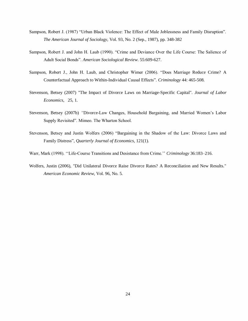
We follow Friedberg‟s (1998) coding of state divorce regimes and the dates of divorce reforms.9 There are

five states that have not yet adopted any form of unilateral divorce: Arkansas, Delaware, Mississippi, New

York and Tennessee. Of the forty-six states that currently have unilateral divorce regimes, eight had adopted

some variant of unilateral divorce before the no-fault revolution during the early 1970s.10

In our analysis we

9 However, our results are robust to alternative divorce coding such as that from Gruber (2004).The most important difference with

Gruber (2004) coding comes from the fact that he considers as “non-adopting” those states that have unilateral divorce as well as separation requirements: Illinois, New Jersey, Ohio, Pennsylvania, South Carolina and the District of Columbia. In our analysis, we define an additional dummy variable that captures whether a state has separation requirements. See Table 1 for details.

10 They are Louisiana, Maryland, North Carolina, Oklahoma, Utah, Vermont, Virginia and West Virginia. These states are coded as

“Pre-1968” in Column 1 of Table 1.

8

consider as “adopting states” those 38 states (including the District of Columbia) that adopted unilateral

divorce in 1968 or later; while the remaining 13 states are considered “control states”.

In the first part of our analysis, we use the natural variation resulting from the different timing of the adoption

of unilateral divorce laws across states to estimate the effects of these laws on aggregate crime and arrest

rates. Consequently, we use state-based panel estimation, including both state and time fixed effects in all

regressions and state-specific trends. We opted for a dynamic specification, allowing the impact to vary by

time since the reform was introduced, in order to differentiate short run from long term impacts of the reform

(Wolfers, 2006).

In the second part of our study, we use age-specific arrest and murder rates. Here we take advantage of an

additional source of variation that comes from the age that a cohort faced the unilateral reform. This second

source of variation allows us first to identify differential effects between individuals that have faced the

reform at different points of their life. Second, since the source of variation is at the state-year of birth level,

we are able to control by confounding factors that might operate at the state-year, state-age or age-year level.

All our regressions are state population weighted.11

Finally, to control for serial correlation, we correct the

standard errors by clustering by state, following Bertrand, Duflo, and Mullainathan (2004).

The crime data in our analysis comes from the FBI´s Uniform Crime Report program (UCR) and from the

Supplemental Homicide Report.12

The UCR data consists of information at the state level for the eight types

of crimes that are considered the most important because of their nature or volume among all offenses (Part I

offenses). These felonies are classified into two groups: Violent Crimes13

and Property Crime. Violent crime

groups four offenses: murder and non-negligent manslaughter, forcible rape, robbery, and aggravated assault.

Property Crime includes the offenses of burglary, larceny-theft, motor vehicle theft, and arson.

Because the FBI data rely on police reporting, there are often problems of underreporting or downgrading of

crimes. However, the use of aggregate information at different levels (state-year, state-year-age or state-year-

11 Similar conclusions we get performing unweighted regressions.

12 The UCR data has information for the whole period 1960-2005 with the exception of NY for which the information is available as

of 1965. Therefore, we restrict the analysis for the period 1965-1998, because for other covariates the information is not available beyond the selected period. Nevertheless, we checked the robustness by estimating a model for the whole period without controls; the results do not change qualitatively.

13 The Uniform Crime Reporting (UCR) Program defines as violent crimes those that involve force or threat of force. The

classification of these offenses is based on police investigation as opposed to the determination of a court, medical examiner, coroner, jury, or other judicial body. For more details, see the Uniform Crime Reporting codebook at http://www.fbi.gov/ucr/handbook/ucrhandbook04.pdf.

9

race) as well as analyzing different types of offenses allow us to draw conclusions based on results that are

less sensitive to measurement errors.14

In this paper we use, first, the crime rates reported at state-year level for the period 1965-1998.15

We also use

data on the number of arrests by type of offense and on homicide counts from the Supplemental Homicide

Report (SHR). The number of arrests reported to the FBI UCR Program each year by police agencies in

metropolitan statistical areas in the United States is disaggregated by age, sex, and race. The age detail is at

single age for 15 to 24 year olds and grouped for the other ages. This level of detail is useful since it allows us

to identify not only the population affected by the reform, but also the potentials channels. The third source of

data consists of homicide offenders from the FBI‟s Supplemental Homicide Reports (SHR). These data are

also available by state, year and single-year of age for the period 1976-1999; unlike the data on FBI UCR

arrests, all ages are identified. The SHR account for approximately 92 percent of all known homicides, and

just under 4 percent of cases lack information on age. The most significant problem in using SHR data to

analyze offender characteristics, however, is the sizable and growing number of unsolved homicides

contained in the data file. In this paper we used the imputation method created by Fox and Zawitz (2004).16

In order to construct the arrest and homicide (SHR) rates, we use three sources of population counts. The

state population by year is from Donohue and Wolfers (2005). We also use population counts disaggregated

by state and age from Census US Intercensal County Population Data, which is available for all years starting

in 1970. We finally use population counts disaggregated by state, year and race from the National Cancer

Institute (SEER Population estimates), available since 1969. (see data Appendix).

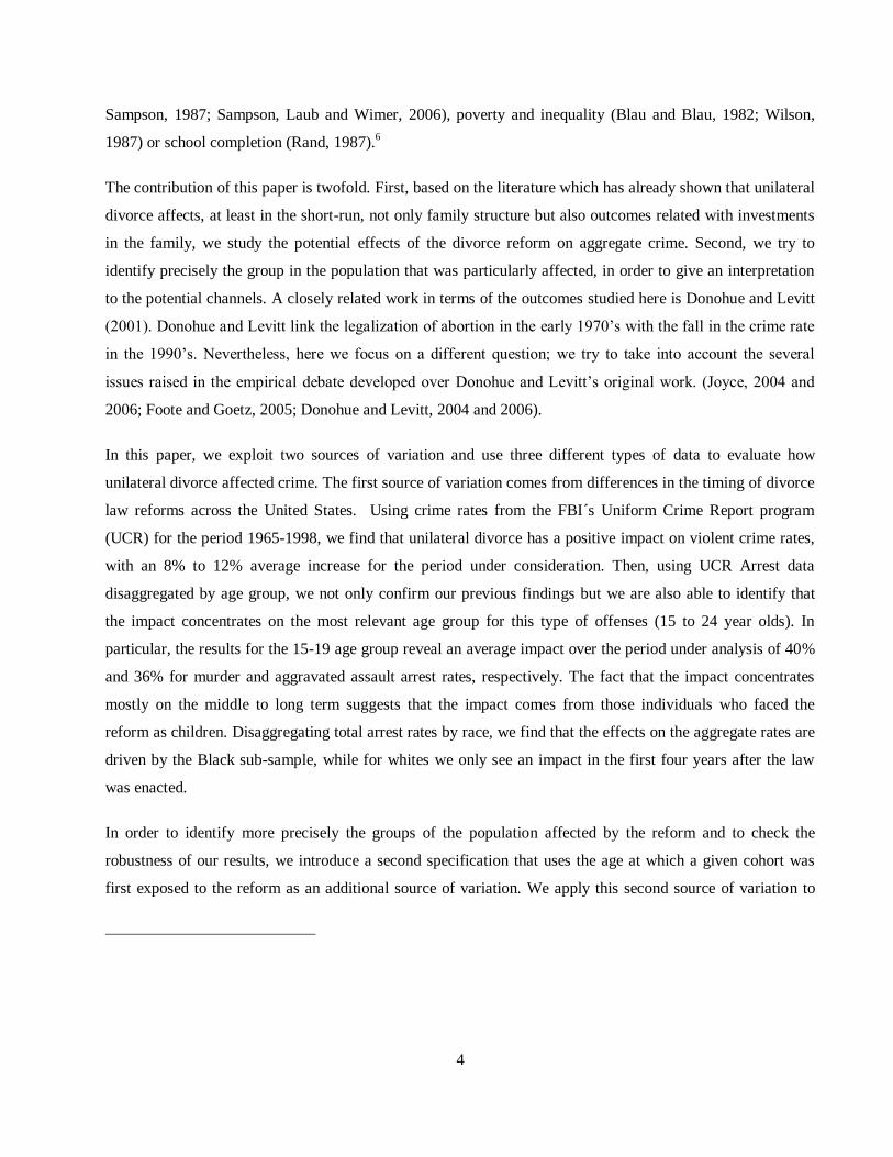
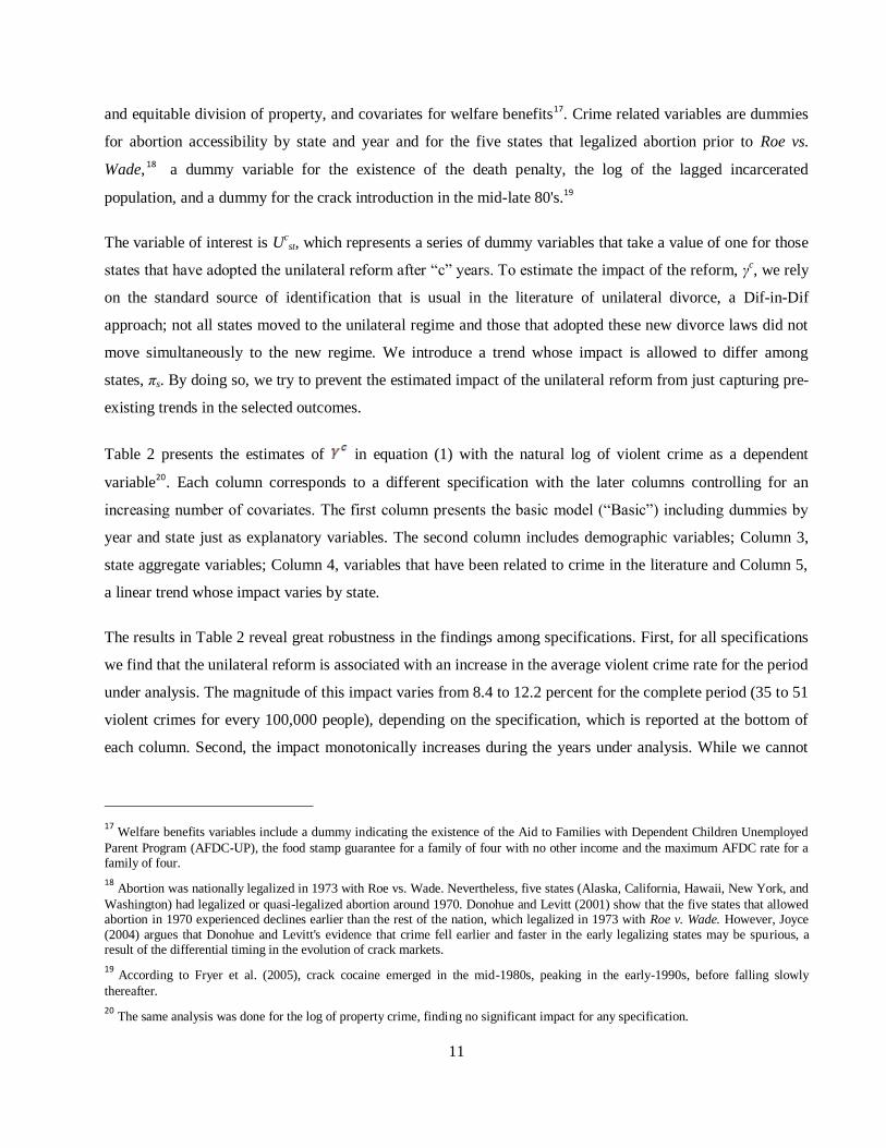
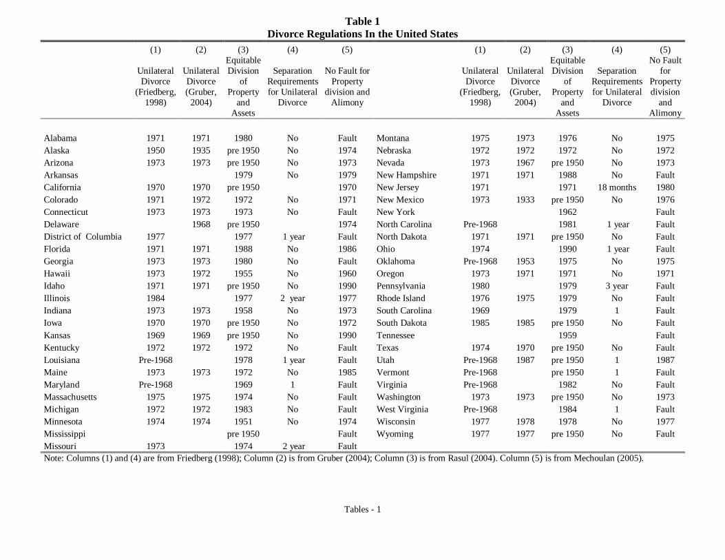
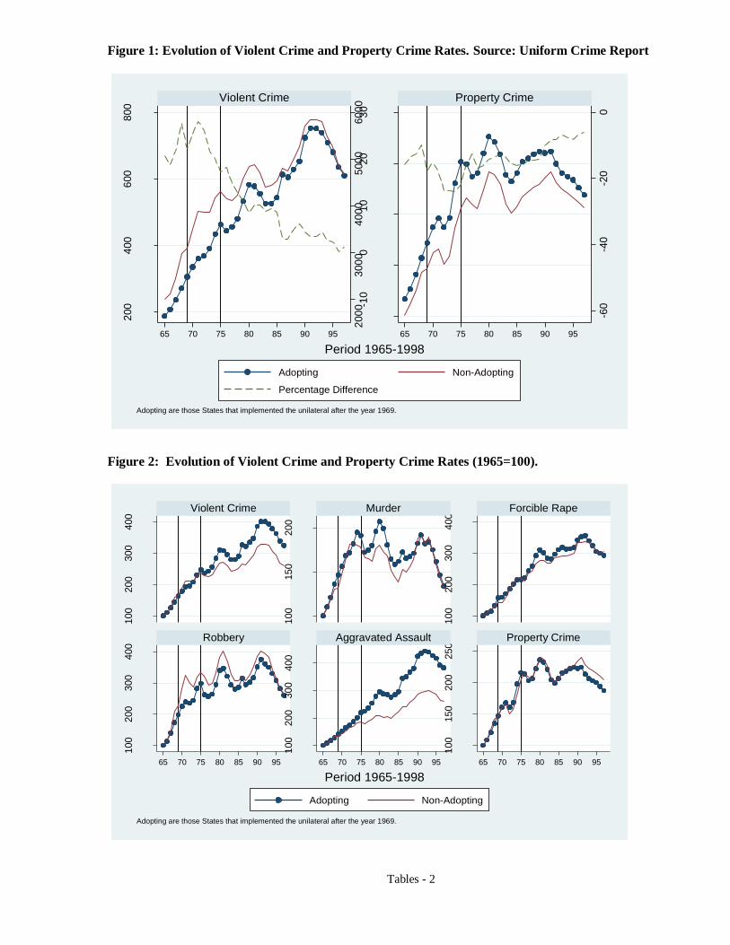
Figure 1 shows the comparative evolution between Adopting and Non-Adopting States for raw Violent and

Property Crime rates, respectively. By “adopting”, we mean states adopting unilateral divorce in 1968 or later.

For each of the panels we introduce two vertical lines signaling the years 1970 and 1975, which indicate the

period that most states adopted the unilateral divorce law (see Table 1). We can see, first, that adopting states

have a lower incidence of violent crimes than non-adopting states. On the other hand, however, adopting

14 Stevenson and Wolfers (2006) check the FBI counts of total murders each year by state against murder counts gathered by the

National Center for Health Statistics (NCHS). They find that these two data sources provide murder counts that are consistent with each other.

15 The UCR data has information for the whole period 1960-2005 with the exception of NY for which the information is available as

of 1965. Therefore, we restrict the analysis to the period 1965-1998, because for other covariates the information is not available beyond the selected period. Nevertheless, we checked the robustness by estimating a model for the whole period without controls; the results do not change qualitatively.

16 With this methodology, offender profiles for unsolved crimes are estimated based on the offender profiles in solved cases matched

by victim age, sex, and race as well as year and state. However, our results are robust to the use of non-imputed offender data.

10

states have higher incidence of property crime for the period under analysis. Second, after (and not before) the

unilateral reform started there is monotonic reduction in the gap in violent crime rates between adopting and

non-adopting with almost no observable difference in the 1990‟s. On the other hand, the gap between

adopting and non-adopting states in terms of property crime rates seems stable during the period, with a

marginal tendency to increase after 1985.

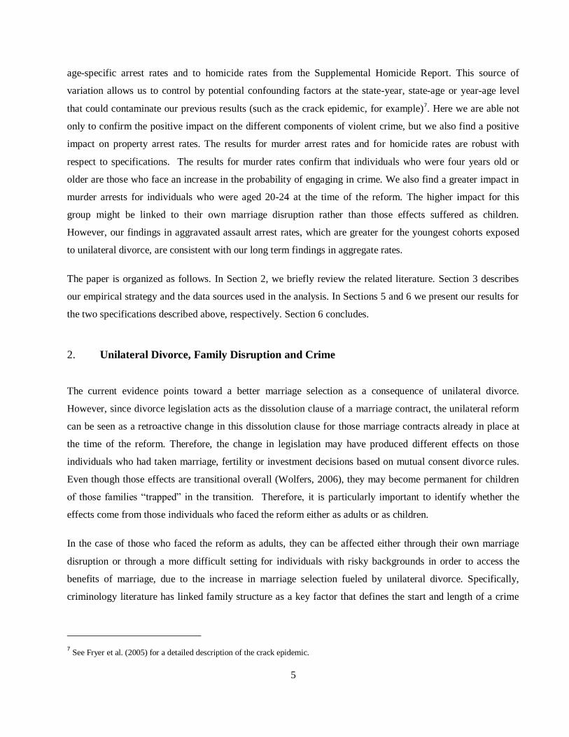
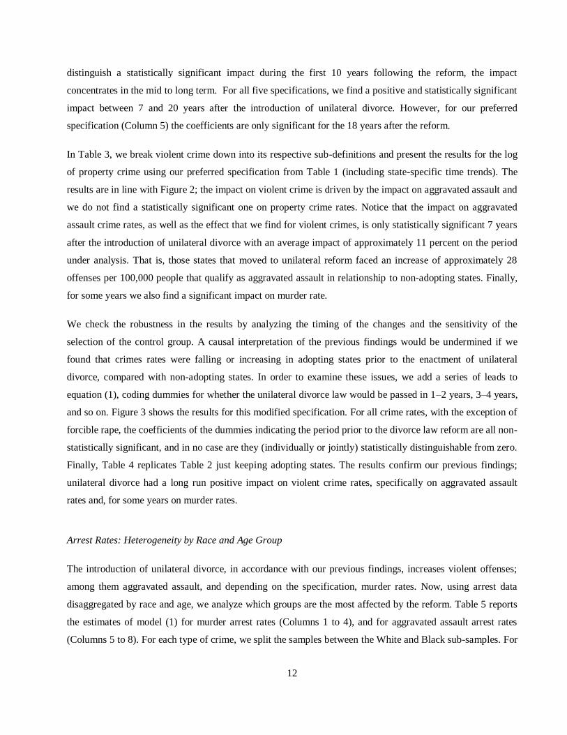
Figure 2 shows violent crime in its different transgressions. In order to stress the evolution during the period

under analysis, we index the different crime rates by using 1965 as base year. Three elements are worth

noting. First, the evolution of violent crimes goes hand in hand with the evolution of aggravated assault,

which is the most significant type of violent crime in terms of volume. Second, adopting states did not begin

catching up in terms of violent crime rates until 1975, which is, at least at a descriptive level, consistent with

non-preexistent trends driving this profile during this period. Third, the faster relative growth of violent crime

rates among adopting states in relation to non-adopting states occurs for the periods 1975-1980 and 1985-

1990. In fact, after 1990 both adopting and non-adopting states follow a similar profile for all violent

transgressions, that is, a well-known and documented drop in crime rates after 1995. Finally, for “Murder”

and “Forcible Rape” offenses, there is a mid–run relative increase among adopting states, which at the end of

the period, however, is not perceptible.

4. Aggregate Crime and Arrest Rates

The following expression represents the first specification of interest,

, (1)

with yst representing one specific crime or arrest rate for state s at time t, δs and ηt, represent state and year

fixed effects, respectively. Finally, Zst stands for time-varying aggregate and policy state variables. Among

these time-varying covariates we distinguish three groups of variables: Demographic variables, State

Aggregate and Policy variables, and finally variables that have been associated with crime by previous

studies. Demographic covariates include the fraction of African-American population living in the state, the

state poverty rate, fraction of foreign-born population, the fraction of people living in metropolitan areas, the

state-year age structure of the population and the interaction of the fraction of African-American population

with the poverty rate, and fraction in a metropolitan area. Policy variables are the log of per capita income, the

unemployment rate, and dummies for the requirement of fault for property division, separation requirements,

11

and equitable division of property, and covariates for welfare benefits17

. Crime related variables are dummies

for abortion accessibility by state and year and for the five states that legalized abortion prior to Roe vs.

Wade,18

a dummy variable for the existence of the death penalty, the log of the lagged incarcerated

population, and a dummy for the crack introduction in the mid-late 80's.19

The variable of interest is Ucst, which represents a series of dummy variables that take a value of one for those

states that have adopted the unilateral reform after “c” years. To estimate the impact of the reform, γc, we rely

on the standard source of identification that is usual in the literature of unilateral divorce, a Dif-in-Dif

approach; not all states moved to the unilateral regime and those that adopted these new divorce laws did not

move simultaneously to the new regime. We introduce a trend whose impact is allowed to differ among

states, πs. By doing so, we try to prevent the estimated impact of the unilateral reform from just capturing pre-

existing trends in the selected outcomes.

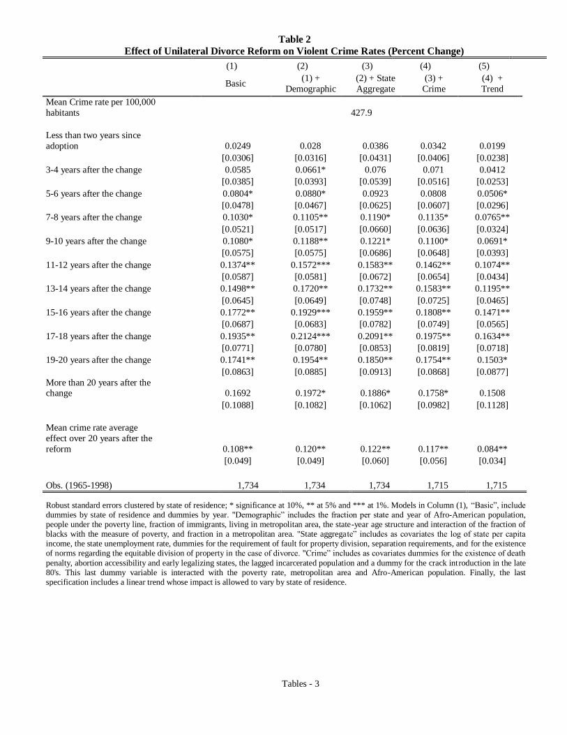
Table 2 presents the estimates of in equation (1) with the natural log of violent crime as a dependent

variable20

. Each column corresponds to a different specification with the later columns controlling for an

increasing number of covariates. The first column presents the basic model (“Basic”) including dummies by

year and state just as explanatory variables. The second column includes demographic variables; Column 3,

state aggregate variables; Column 4, variables that have been related to crime in the literature and Column 5,

a linear trend whose impact varies by state.

The results in Table 2 reveal great robustness in the findings among specifications. First, for all specifications

we find that the unilateral reform is associated with an increase in the average violent crime rate for the period

under analysis. The magnitude of this impact varies from 8.4 to 12.2 percent for the complete period (35 to 51

violent crimes for every 100,000 people), depending on the specification, which is reported at the bottom of

each column. Second, the impact monotonically increases during the years under analysis. While we cannot

17 Welfare benefits variables include a dummy indicating the existence of the Aid to Families with Dependent Children Unemployed

Parent Program (AFDC-UP), the food stamp guarantee for a family of four with no other income and the maximum AFDC rate for a family of four.

18 Abortion was nationally legalized in 1973 with Roe vs. Wade. Nevertheless, five states (Alaska, California, Hawaii, New York, and

Washington) had legalized or quasi-legalized abortion around 1970. Donohue and Levitt (2001) show that the five states that allowed abortion in 1970 experienced declines earlier than the rest of the nation, which legalized in 1973 with Roe v. Wade. However, Joyce

(2004) argues that Donohue and Levitt's evidence that crime fell earlier and faster in the early legalizing states may be spurious, a result of the differential timing in the evolution of crack markets.

19 According to Fryer et al. (2005), crack cocaine emerged in the mid-1980s, peaking in the early-1990s, before falling slowly

thereafter.

20 The same analysis was done for the log of property crime, finding no significant impact for any specification.

12

distinguish a statistically significant impact during the first 10 years following the reform, the impact

concentrates in the mid to long term. For all five specifications, we find a positive and statistically significant

impact between 7 and 20 years after the introduction of unilateral divorce. However, for our preferred

specification (Column 5) the coefficients are only significant for the 18 years after the reform.

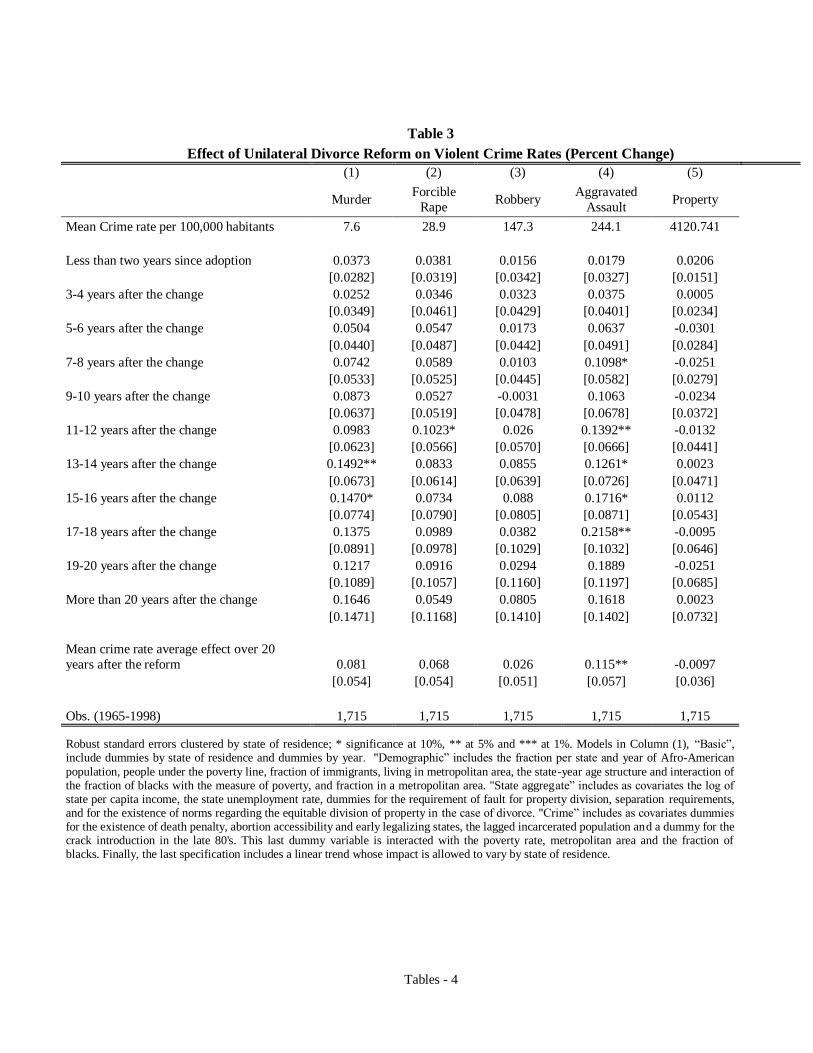
In Table 3, we break violent crime down into its respective sub-definitions and present the results for the log

of property crime using our preferred specification from Table 1 (including state-specific time trends). The

results are in line with Figure 2; the impact on violent crime is driven by the impact on aggravated assault and

we do not find a statistically significant one on property crime rates. Notice that the impact on aggravated

assault crime rates, as well as the effect that we find for violent crimes, is only statistically significant 7 years

after the introduction of unilateral divorce with an average impact of approximately 11 percent on the period

under analysis. That is, those states that moved to unilateral reform faced an increase of approximately 28

offenses per 100,000 people that qualify as aggravated assault in relationship to non-adopting states. Finally,

for some years we also find a significant impact on murder rate.

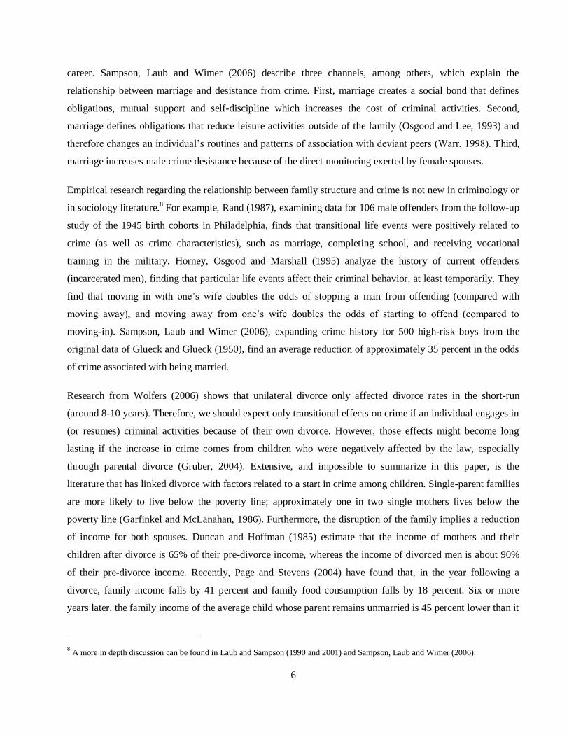
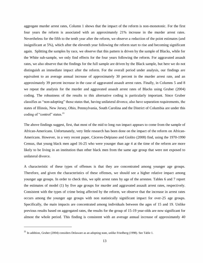
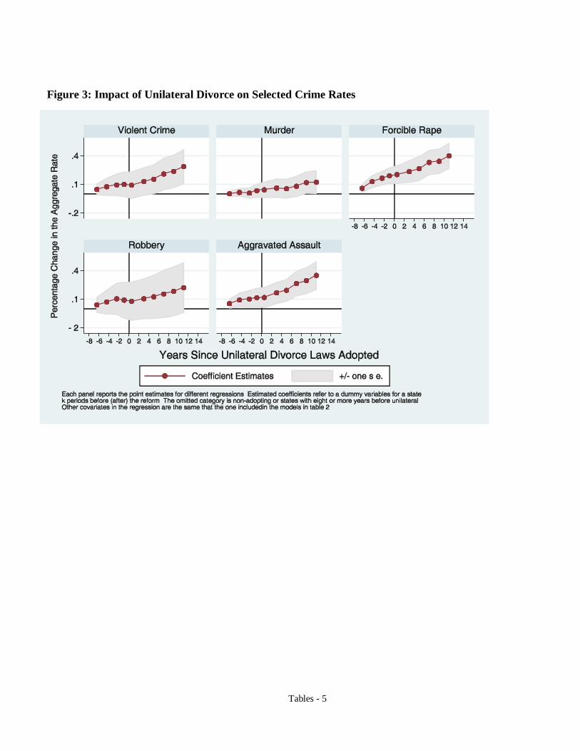
We check the robustness in the results by analyzing the timing of the changes and the sensitivity of the

selection of the control group. A causal interpretation of the previous findings would be undermined if we

found that crimes rates were falling or increasing in adopting states prior to the enactment of unilateral

divorce, compared with non-adopting states. In order to examine these issues, we add a series of leads to

equation (1), coding dummies for whether the unilateral divorce law would be passed in 1–2 years, 3–4 years,

and so on. Figure 3 shows the results for this modified specification. For all crime rates, with the exception of

forcible rape, the coefficients of the dummies indicating the period prior to the divorce law reform are all non-

statistically significant, and in no case are they (individually or jointly) statistically distinguishable from zero.

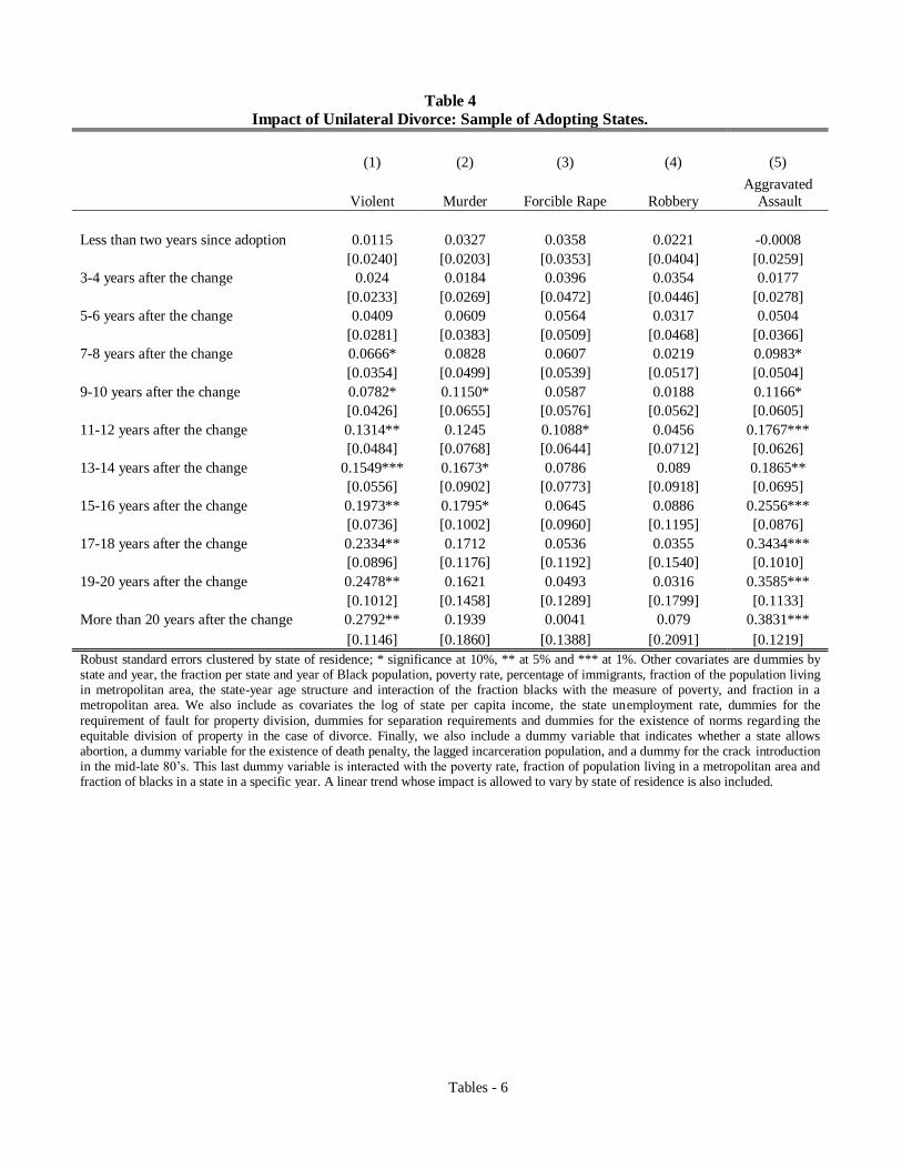
Finally, Table 4 replicates Table 2 just keeping adopting states. The results confirm our previous findings;

unilateral divorce had a long run positive impact on violent crime rates, specifically on aggravated assault

rates and, for some years on murder rates.

Arrest Rates: Heterogeneity by Race and Age Group

The introduction of unilateral divorce, in accordance with our previous findings, increases violent offenses;

among them aggravated assault, and depending on the specification, murder rates. Now, using arrest data

disaggregated by race and age, we analyze which groups are the most affected by the reform. Table 5 reports

the estimates of model (1) for murder arrest rates (Columns 1 to 4), and for aggravated assault arrest rates

(Columns 5 to 8). For each type of crime, we split the samples between the White and Black sub-samples. For

13

aggregate murder arrest rates, Column 1 shows that the impact of the reform is non-monotonic. For the first

four years the reform is associated with an approximately 21% increase in the murder arrest rates.

Nevertheless for the fifth to the tenth year after the reform, we observe a reduction of the point estimates (and

insignificant at 5%), which after the eleventh year following the reform start to rise and becoming significant

again. Splitting the samples by race, we observe that this pattern is driven by the sample of Blacks, while for

the White sub-sample, we only find effects for the four years following the reform. For aggravated assault

rates, we also observe that the findings for the full sample are driven by the Black sample, but here we do not

distinguish an immediate impact after the reform. For the overall period under analysis, our findings are

equivalent to an average annual increase of approximately 30 percent in the murder arrest rate, and an

approximately 39 percent increase in the case of aggravated assault arrest rates. Finally, in Columns 5 and 8

we repeat the analysis for the murder and aggravated assault arrest rates of Blacks using Gruber (2004)

coding. The robustness of the results to this alternative coding is particularly important. Since Gruber

classifies as “non-adopting” those states that, having unilateral divorce, also have separation requirements, the

states of Illinois, New Jersey, Ohio, Pennsylvania, South Carolina and the District of Columbia are under this

coding of “control” states.21

The above findings suggest, first, that most of the mid to long run impact appears to come from the sample of

African-Americans. Unfortunately, very little research has been done on the impact of the reform on African-

Americans. However, in a very recent paper, Cáceres-Delpiano and Giolito (2008) find, using the 1970-1990

Census, that young black men aged 16-25 who were younger than age 4 at the time of the reform are more

likely to be living in an institution than other black men from the same age group that were not exposed to

unilateral divorce.

A characteristic of these types of offenses is that they are concentrated among younger age groups.

Therefore, and given the characteristics of these offenses, we should see a higher relative impact among

younger age groups. In order to check this, we split arrest rates by age of the arrestee. Tables 6 and 7 report

the estimates of model (1) by five age groups for murder and aggravated assault arrest rates, respectively.

Consistent with the types of crime being affected by the reform, we observe that the increase in arrest rates

occurs among the younger age groups with non statistically significant impact for over-25 age groups.

Specifically, the main impacts are concentrated among individuals between the ages of 15 and 19. Unlike

previous results based on aggregated rates, the results for the group of 15-19 year-olds are now significant for

almost the whole period. This finding is consistent with an average annual increase of approximately 40

21 In addition, Gruber (2004) considers Delaware as an adopting state, unlike Friedberg (1998). See Table 1.

14

percent in the murder arrest rate (an increase of approximately 5 annual arrests per 100,000 people), and an

approximately 35 percent increase in the average annual rate for aggravated assault (an annual increase of 60

arrests per 100,000 habitants). For the group of 20-24 year olds we observe that the impact of unilateral

divorce is only present for the first 4 years after the reform and for the period 13 to 14 years after its

introduction in the case of murder arrest rates, with no significant impact for any period in the case of

aggravated assault. This pattern is consistent with an earlier start in relatively less serious offenses like

aggravated assault, and a later escalation to more serious offenses like murder. The lack of a significant

impact beyond the fourth year after the reform for the murder arrest rate for the age groups 15-19 and 20-24

might be mechanical. An earlier arrest implies that some individuals are locked up for a time, preventing them

from engaging in crime. For the period 1981-1995 the average time served for juveniles convicted for murder

was approximately 112 months (approximately 9 years)22

, which almost matches the 8 years in which we do

not observe an impact until the period 13 to 14 years after the introduction of unilateral divorce when younger

cohorts arrive on the scene. Evidence in criminology is consistent with our findings. The types of crime

affected by the reform and the timing of these impacts provide some explanation about the channels through

which the reform is affecting crime. Family structure is an element producing desistance from crime but its

impact on crime depends on the point in the life cycle in which it occurs. Divorce not only increases the

chances of a longer crime career but also increases the chances of more serious offenses (Laub and Sampson,

2001). Our findings of mid to long term impact on violent-crimes are consistent with an effect on younger

age groups who are negatively affected by the reform as children (Gruber, 2004; Cáceres-Delpiano and

Giolito, 2008). In the next section, we further investigate this hypothesis by analyzing age-specific arrest and

murder rates. In fact, this consequent increase in the likelihood of falling into crime earlier is by itself a

predictor of committing serious offenses (violent crime). We investigate these hypotheses in more detail in

the next section.

5. Age-Specific Arrest and Homicide Rates

The evidence so far points towards an impact of unilateral divorce on violent crime (murder and aggravated

assault), principally in the mid to long term for the 15-24 age group. The analysis by race showed that the

findings for the aggregate rates appear to follow closely from the ones for Blacks sub-sample. In this section,

we introduce a second specification that allows us, first, to identify more precisely the group of the population

most affected by the reform and, second, to introduce additional controls to check the robustness of previous

22 Bureau of Justice Statistics, U.S. Department of Justice. http://www.ojp.usdoj.gov/bjs/pub/html/cjusew96/ts.htm .

15

results. We concentrate on age-specific arrests and murder (SHR) rates of the population aged 15-24, since

the Uniform Crime Reports record arrests by single year of age for this group only. In order to construct age-

specific arrest and homicide rates we rely on the single-age population counts from the Census US Intercensal

County Population Data, which is available for all years starting in 1970 (see data Appendix). Therefore, we

restrict our analysis on age-specific arrest rates to the period starting in 1970.23

Our second specification is

the following:

, (2)

with yast now representing a crime rate for the population of age a, living in state s at year t.24

Here , , ,

and represent state, year, age, state-year, age-year and state-age fixed effects, respectively.

Furthermore, is a dummy variable representing whether abortion was already legalized in state s in

the year of birth of population that is a years old at time t; 1{*} is an indicator function that takes a value of

one when the logic statement * is true, and zero otherwise. YBast is the year of birth for individuals of age a at

time t living in the state s; YUnis is the year of adoption of unilateral divorce in the state s. That is,

represents the age at the time of introduction of the reform. The parameter of interest, , can be

interpreted as the ceteris paribus contribution of unilateral divorce of those cohorts of ages in the range

[ at the time of the reform, compared to those individuals living in states that have not adopted

unilateral divorce . Seven age groups at the time of the introduction of unilateral divorce are

defined; Born after the reform > 0), between 0 and 3 years old at the time of the reform,

between 4 and 7, 8 and 11 and so on. In this last specification, three are the source of variation of the variable

associated to the parameter . In addition to the differences in the timing of adoption of unilateral divorce

and the fact that not all states have introduced it, we use in the specification the fact that the reform affected

individuals at different points in their lives.

This specification also allows us to control for confounding factors that vary on the state-year level, that is,

they affect everyone within a state in a particular year. One example of these factors are the temporary state-

specific crime waves such us the introduction of new, illicit drugs, such as crack cocaine (Donohue and

Levitt, 2001, 2004, 2006; Joyce, 2004, Foote and Goetz, 2005). Given that here the source of variation is by

23 However, we obtain similar results if we construct rates back to 1965 by using linear interpolations of Census data.

24 Due to the high number of zeros in age-specific crime data, here we calculate elasticities evaluated at the sample mean instead of

using logs, as we did in previous sections.

16

state-year-age, we are able to introduce state-year, state-age and age-year interactions (Foote and Goetz, 2005;

Donohue and Levitt, 2006) and therefore remove any confounding effect operating at the state-year level,

state-age level or year-age level.

Table 8 presents the results for murder, robbery, aggravated assault, violent and property arrest rates using our

second specification. First, in contrast to our previous specifications, we now also find a significant impact for

robbery and property arrest rates. Nevertheless, the relative impact is still more important for murder and

aggravated assault arrest rates. Second, the coefficients for murder arrest rates are only significant for those

individuals aged 4 years old or more at the time of the reform, with higher point estimates for those aged 20-

24 when the law was passed. A similar pattern appears for robbery rates, significant for those who were older

than 12. However, for aggravated assault the coefficients are increasing for the younger the individuals were

at the time of the reform.

As we already mentioned, murder information, in general, is less likely than other types of offenses to suffer

from measurement problems. The robustness for murder rates is shown in Table 9, which presents the

estimates for murder arrest rates with each column representing a different specification. Observe that the

results are virtually the same when we replace the variable “legal” by directly including the abortion rates at

the year of birth (Donohue and Levitt, 2001, 2004, 2006). We also check our results by considering two

alternative unilateral divorce codings: Friedberg (1998) without separation requirements (i.e. the states that

require time of separation in order to grant a divorce are considered non-adopting) and Gruber (2004).25

In all

cases, the point estimates for individuals who were 20-24 years old at the time of the reform are considerably

higher than the coefficients for other age groups.

Finally, in Table 10, we also verify the robustness of our findings in murder arrest rates using homicide rates

constructed from SHR data, available from 1976 to 1999. The results are very similar to those from arrest

data, except that we do not observe the increase in the estimates for those individuals aged 20-24 at the time

of the reform, probably because the period under analysis starts six years later.

When analyzing the murder arrest rates for the age group 15-24 by the timing since adoption of the law (Table

6, Columns 1 to 3), we find a significant increase in the first four years after the reform. The short-run

increase for individuals aged 20-24 in Table 6 is equivalent to the result for those aged 20-24 at the time of

the reform we showed in Table 9. This group is the least likely to be affected by parental family disruption

25 Gruber (2004) considers unilateral divorce only in the case where there are no separation requirements.

17

because of the reform. In fact, some of these individuals could have already left the parents‟ household when

unilateral divorce was introduced. The higher impact for this group might be linked to their own marriage

disruption, or the greater selection into marriage caused by the law (Stevenson, 2007, Rasul, 2004) that may

have prevented some marginal individuals from the benefits of marriage, a key factor in criminal desistance

according to the criminology literature (Sampson, Laub and Wimer, 2006).

It is also worth noticing that the point estimates for murder arrests and SHR homicide rates (Tables 9 and 10)

do not show a significant impact for those groups born after the reform. This lack of significance raises some

doubts about the long-term effects (more than 20 years after the reform) that are shown in Table 6 for the age

group 15 to 19. Since we are now controlling for confounding factors at the state-year level, we may interpret

that the negative effects fade for children born after the reform, consistent with a better selection into

marriage and the decrease in the divorce rates 10 years after the reform. However, our findings in aggravated

assault arrest rates, which appear to be increasing for the youngest cohorts exposed to unilateral divorce, are

consistent with the long run increase in aggregate arrest rates (Table 5 and Table 7, Column 2), and therefore

striking.

6. Conclusion

In this paper, we study the impact of unilateral divorce on crime. Previous research has suggested that divorce

laws affected marriage selection and produced some negative effects on individuals who faced the reform as

children. Here we study whether those changes affected crime and arrest rates in states that passed unilateral

divorce laws.

First, using data from the FBI´s Uniform Crime Report program for the period 1965-1998 and differences in

the timing in the introduction of the reform we find that unilateral divorce has a positive impact on violent

crime rates, with an 8% to 12% average increase for the period under consideration. The analysis using arrest

data not only confirms the findings of a positive impact on violent crime but also that these impacts are

concentrated among those age groups (15 to 24) which are more likely to engage in these type of offenses.

Specifically for the group of 15-19 year olds, we observe an average impact over the period under analysis of

40% and 36% for murder and aggravated assault arrest rates, respectively. When we disaggregate the arrest

rates by race, we find the results are driven by the Black sub-sample, while for the White sub-sample, we only

find effects for the four years following the reform.

18

We finally analyze age-specific arrest and murder rates using the age at the reform as the second source of

variation. We are not only able to confirm the positive impact on different types of violent crime but we also

find a positive impact for property crimes. The results for murder arrest rates for the period 1970-1997 and for

homicide rates for the period 1976-1999 (Supplemental Homicide Report) are robust with respect to

specifications, specifically those that include year-state and year-age dummies. The results confirm, except

for the case of aggravated assault, that individuals who were already born at the time of the reform (aged 4

and older for murder) are the ones who face the increase in the probability of engaging in crime. The

magnitude goes from 15% to 40% depending on the specification and age at the time of the reform.

19

Data Appendix

Unilateral Divorce Coding

The coding for unilateral divorce and separation requirements comes from Friedberg (1998). The coding for

equitative division of property is from Rasul (2004). The coding for requirements of fault regarding property

division is from Mechoulan (2005). See Table 1 for details.

Aggregate Crime and Arrest Data

Aggregate crime and arrest data used in the analysis are from FBI´s Uniform Crime Report program (UCR)

for the period 1965-1998. The UCR data has information for the whole period 1960-2005 with the exception

of New York (since 1965). The data on crime rates is available from the Bureau of Justice Statistics web

page:

http://bjsdata.ojp.usdoj.gov/dataonline/Search/Crime/State/StatebyState.cfm

Arrest data is from Chilton and Weber (2000), available from the Inter-University Consortium for Political

and Social Research (ICPSR) web page: http://www.icpsr.umich.edu.

Supplemental Homicide Reports (SHR)

Data from SHR is from Fox (2004), available from the ICPSR web page: http://www.icpsr.umich.edu.

Prisoners, and Death Penalty

Data on number of prisoners and the existence of death penalty are from Donohue and Wolfers (2005),

available at Justin Wolfers‟ web page: http://bpp.wharton.upenn.edu/jwolfers/DeathPenalty.shtml. The

variable indicating the stock of incarcerated people have same states missing for the years 1965, 1968 and

1970-72.

Population

Population counts by year and state are taken form Donohue and Wolfers (2005). For counts at year-state-age

level, we use the Census US Intercensal Population Data, which is available for all years starting in 1970. The

data is available at the NBER website: http://www.nber.org/data/census-intercensal-population/

20

For population counts at the state-race-year level, we use data from the National Cancer Institute, Surveillance

Epidemiology and End Results, available at http://seer.cancer.gov/popdata/download.html. For the period

1965-1969, we make a linear interpolation using IPUMS Census data for the years 1960 and 1970.

Abortion Rates

Data on abortion rates by state and year is from Donohue and Levitt (2006), available from John J. Donohue

web page: http://islandia.law.yale.edu/donohue/pubsdata.htm.

Welfare Generosity, Unemployment rate, and Log of per capita Income

The data is from the “Moffit Benefits File”, available from Robert Moffit‟s web page:

http://www.econ.jhu.edu/people/moffitt/ben_data.txt.

Demographic Covariates

The share of Population living in Metropolitan areas , fraction of people below the poverty line, fraction of

blacks and the age structure of the population (5-year cohorts) are constructed from March CPS data starting

in 1977. Since for previous years some states are grouped in March CPS, we make a lineal interpolation using

IPUMS census data. The share of foreign-born population is also by linear interpolation of census data

21

References

Alesina, Alberto and Paola Giuliano (2007), “Divorce, Fertility and the Value of Marriage”. Mimeo. Harvard

University.

Bertrand, Marianne, Esther Duflo, and Sendhil Mullainathan (2004), “How much should we trust differences-

in-differences estimates?” Quarterly Journal of Economics 119, no. 1:249–75.

Blau, Judith R., and Peter M. Blau (1982), “The Cost of Inequality: Metropolitan Structure and Violent

Crime”. American Sociological Review, Vol. 47, No. 1. (Feb., 1982), pp. 114-129.

Cáceres-Delpiano, Julio, and Eugenio Giolito (2008), "How Unilateral Divorce Affects Children". IZA

Discussion Paper No. 3342.

Chiappori, Pierre André, Bernard Fortin, and Guy Lacroix (2002), "Marriage Market, Divorce Legislation,

and Household Labor Supply." Journal of Political Economy, 85 (6), 1141-1187.

Chilton, Roland, and Dee Weber (2000), Uniform Crime Reporting Program Data [United States]: Arrests by

Age, Sex, and Race for Police Agencies in Metropolitan Statistical Areas, 1960-1997 [Computer file].

2nd ICPSR version. Amherst, MA: University of Massachusetts [producer], 2000. Ann Arbor, MI:

Inter-university Consortium for Political and Social Research [distributor].

Dee, Thomas S. (2003) “Until death do you part: The effects of unilateral divorce on spousal homicides”,

Economic Inquiry; 41, 1.

Donohue, John J. and Steven Levitt (2001), “The Impact of Legalized Abortion on Crime”, Quarterly Journal

of Economics 116(2):379-420.

Donohue, John J. and Steven Levitt (2004), “Further Evidence that Legalized Abortion Lowered Crime: A

Reply to Joyce”, Journal of Human Resources 39(1):29-49.

Donohue, John J., and Steven Levitt (2006), “Measurement Error, Legalized Abortion, and the Decline in

Crime: A Response to Foote and Goetz (2005)”, Working Paper.

Donohue, John J., and Justin Wolfers (2005), “Uses and Abuses of Empirical Evidence in the Death Penalty

Debate”, Stanford Law Review 58:791-846.

22

Drewianka, Scott (2004). "Divorce Law and Family Formation". Journal of Population Economics,

forthcoming.

Foote, Christopher, and Christopher Goetz (2005), “The Impact of Legalized Abortion on Crime: Comment.”,

Quarterly Journal of Economics, forthcoming

Friedberg, Leora (1998) "Did Unilateral Divorce Raise Divorce Rates? Evidence from Panel Data," American

Economic Review, 88, 608-627.

Fryer, Roland, Paul Heaton, Steven Levitt and Kevin Murphy (2005). “Measuring the Impact of Crack

Cocaine.” NBER Working Papers Series no. 11318; Cambridge: National Bureau of Economic

Research.

Fox, James Alan. (2004). “Uniform Crime Reports [United States]: Supplemental Homicide Reports, 1976-

1998.” [Computer File]. Inter-University Consortium for Political and Social Research versions.

Boston, MA: Northeastern University, College of Criminal Justice [producer]; Ann Arbor: Michigan:

Inter-University Consortium for Political and Social Research [distributor].

Fox, James Alan, and Marianne W. Zawitz, (2004), “Weighting and Imputation Procedures for 1976-2002

Cumulative Data File. http://www.ojp.usdoj.gov/bjs/homicide/imputationandweighting.htm.

Ginther, Donna K., and Robert Pollak (2004), “Family Structure and Children's Educational Outcomes:

Blended Families, Stylized Facts, and Descriptive Regressions”. Demography - Volume 41, Number

4, November 2004, pp. 671-696

Goldin, Claudia, and Lawrence F. Katz (2002). “The Power of the Pill: Oral Contraceptives and Women‟s

Career and Marriage Decisions”. Journal of Political Economy, vol. 110, no. 4]

Gray, Jeffrey S. (1998), "Divorce-Law Changes, Household bargaining, and Married Women's Labor

Supply." American Economic Review, 88 (3), 628-642.

Glueck, Sheldon, and Eleanor Glueck (1950). Unraveling Juvenile Delinquency. New York: Commonwealth

Fund.

Gruber, Jonathan (2004), "Is making Divorce Easier Bad for Children?”. Journal of Labor Economics, 22 (4),

799-833.

23

Haveman, Robert, and Barbara Wolfe (1995), “The determinants of children's attainments: A review of

methods and findings”. Journal of Economic Literature 33, pp. 1829–1979.

Horney, Julie, D. Wayne Osgood and Ineke Marshall (1995). "Criminal Careers in the Short-Term: Intra-

Individual Variability in Crime and its relation to Local Life Circumstances." American Sociological

Review, 60, 655-673.

Johnson, John, and Christopher Mazingo (2000). "The Economic Consequences of Unilateral Divorce for

Children." University of Illinois Office of Research Working paper.

Joyce, Ted (2004), “Did Legalized Abortion Lower Crime?” Journal of Human Resources 39(1):1-28.

Joyce, Ted (2006), “A Simple Test of Abortion and Crime”. Review of Economics and Statistics, forthcoming.

Matsueda, Ross L, and Karen Heimer (1987), “Race, Family Structure, and Delinquency: A Test of

Differential Association and Social Control Theories”. American Sociological Review, Vol. 52, No. 6,

826-840.

Mechoulan, Stéphane (2005), Economic Theory‟s Stance on No-Fault Divorce, Review of the Economics of

the Household 3: 337-359.

Mechoulan, Stéphane (2006), Divorce Laws and the Structure of the American Family, Journal of Legal

Studies 35(1): 143-174.

McLanahan, Sara, and Karen Booth (1989), “Mother-Only Families: Problems, Prospects, and Politics,”

Journal of Marriage and the Family 51(3): 557-580.

Osgood, D. Wayne, and Hyunkee Lee (1993). „„Leisure Activities, Age, and Adult Roles across the

Lifespan‟‟. Society and Leisure 16:181–208.

Peters, H. Elizabeth (1986), "Marriage and Divorce: Informational Constraints and Private Contracting."

American Economic Review, 76 (3), 437-454.

Rand, Alicia (1987). „„Transitional Life Events and Desistance from Delinquency and Crime.‟‟ In From Boy

to Man, from Delinquency to Crime, edited by Marvin E. Wolfgang, Terence P. Thornberry, and

Robert M. Figlio. Chicago: University of Chicago Press.

Rasul, Imran (2004), "The Impact of Divorce Laws on Marriage". Mimeo. University of Chicago.

24

Sampson, Robert J. (1987) “Urban Black Violence: The Effect of Male Joblessness and Family Disruption”.

The American Journal of Sociology, Vol. 93, No. 2 (Sep., 1987), pp. 348-382

Sampson, Robert J. and John H. Laub (1990). “Crime and Deviance Over the Life Course: The Salience of

Adult Social Bonds”. American Sociological Review. 55:609-627.

Sampson, Robert J., John H. Laub, and Christopher Wimer (2006). “Does Marriage Reduce Crime? A

Counterfactual Approach to Within-Individual Causal Effects”. Criminology 44: 465-508.

Stevenson, Betsey (2007) "The Impact of Divorce Laws on Marriage-Specific Capital". Journal of Labor

Economics, 25, 1.

Stevenson, Betsey (2007b) “Divorce-Law Changes, Household Bargaining, and Married Women‟s Labor

Supply Revisited”. Mimeo. The Wharton School.

Stevenson, Betsey and Justin Wolfers (2006) “Bargaining in the Shadow of the Law: Divorce Laws and

Family Distress”, Quarterly Journal of Economics, 121(1).

Warr, Mark (1998). „„Life-Course Transitions and Desistance from Crime.‟‟ Criminology 36:183–216.

Wolfers, Justin (2006), "Did Unilateral Divorce Raise Divorce Rates? A Reconciliation and New Results."

American Economic Review, Vol. 96, No. 5.

Tables - 1

Table 1

Divorce Regulations In the United States

(1) (2) (3) (4) (5) (1) (2) (3) (4) (5)

Unilateral

Divorce

(Friedberg,

1998)

Unilateral

Divorce

(Gruber,

2004)

Equitable

Division

of

Property

and

Assets

Separation

Requirements

for Unilateral

Divorce

No Fault for

Property

division and

Alimony

Unilateral

Divorce

(Friedberg,

1998)

Unilateral

Divorce

(Gruber,

2004)

Equitable

Division

of

Property

and

Assets

Separation

Requirements

for Unilateral

Divorce

No Fault

for

Property

division

and

Alimony

Alabama 1971 1971 1980 No Fault Montana 1975 1973 1976 No 1975

Alaska 1950 1935 pre 1950 No 1974 Nebraska 1972 1972 1972 No 1972

Arizona 1973 1973 pre 1950 No 1973 Nevada 1973 1967 pre 1950 No 1973

Arkansas 1979 No 1979 New Hampshire 1971 1971 1988 No Fault

California 1970 1970 pre 1950 1970 New Jersey 1971 1971 18 months 1980

Colorado 1971 1972 1972 No 1971 New Mexico 1973 1933 pre 1950 No 1976

Connecticut 1973 1973 1973 No Fault New York 1962 Fault

Delaware 1968 pre 1950 1974 North Carolina Pre-1968 1981 1 year Fault

District of Columbia 1977 1977 1 year Fault North Dakota 1971 1971 pre 1950 No Fault

Florida 1971 1971 1988 No 1986 Ohio 1974 1990 1 year Fault

Georgia 1973 1973 1980 No Fault Oklahoma Pre-1968 1953 1975 No 1975

Hawaii 1973 1972 1955 No 1960 Oregon 1973 1971 1971 No 1971

Idaho 1971 1971 pre 1950 No 1990 Pennsylvania 1980 1979 3 year Fault

Illinois 1984 1977 2 year 1977 Rhode Island 1976 1975 1979 No Fault

Indiana 1973 1973 1958 No 1973 South Carolina 1969 1979 1 Fault

Iowa 1970 1970 pre 1950 No 1972 South Dakota 1985 1985 pre 1950 No Fault

Kansas 1969 1969 pre 1950 No 1990 Tennessee 1959 Fault

Kentucky 1972 1972 1972 No Fault Texas 1974 1970 pre 1950 No Fault

Louisiana Pre-1968 1978 1 year Fault Utah Pre-1968 1987 pre 1950 1 1987

Maine 1973 1973 1972 No 1985 Vermont Pre-1968 pre 1950 1 Fault

Maryland Pre-1968 1969 1 Fault Virginia Pre-1968 1982 No Fault

Massachusetts 1975 1975 1974 No Fault Washington 1973 1973 pre 1950 No 1973

Michigan 1972 1972 1983 No Fault West Virginia Pre-1968 1984 1 Fault

Minnesota 1974 1974 1951 No 1974 Wisconsin 1977 1978 1978 No 1977

Mississippi pre 1950 Fault Wyoming 1977 1977 pre 1950 No Fault

Missouri 1973 1974 2 year Fault

Note: Columns (1) and (4) are from Friedberg (1998); Column (2) is from Gruber (2004); Column (3) is from Rasul (2004). Column (5) is from Mechoulan (2005).

Tables - 2

Figure 1: Evolution of Violent Crime and Property Crime Rates. Source: Uniform Crime Report

Figure 2: Evolution of Violent Crime and Property Crime Rates (1965=100).

-10

01

02

03

0

-60

-40

-20

0

200

400

600

800

200

03

00

04

00

05

00

06

00

0

65 70 75 80 85 90 95 65 70 75 80 85 90 95

Violent Crime Property Crime

Adopting Non-Adopting

Percentage Difference

Num

ber

of C

rim

es p

er

100 T

ho

usand P

eo

ple

Period 1965-1998

Adopting are those States that implemented the unilateral after the year 1969.

100

200

300

400

100

150

200

100

200

300

400

100

200

300

400

100

200

300

400

100

150

200

250

65 70 75 80 85 90 95 65 70 75 80 85 90 95 65 70 75 80 85 90 95

Violent Crime Murder Forcible Rape

Robbery Aggravated Assault Property Crime

Adopting Non-Adopting

Cri

me Index 1

965=

10

0

Period 1965-1998

Adopting are those States that implemented the unilateral after the year 1969.

Tables - 3

Table 2 Effect of Unilateral Divorce Reform on Violent Crime Rates (Percent Change)

(1) (2) (3) (4) (5)

Basic

(1) +

Demographic

(2) + State

Aggregate

(3) +

Crime

(4) +

Trend

Mean Crime rate per 100,000

habitants 427.9

Less than two years since

adoption 0.0249 0.028 0.0386 0.0342 0.0199

[0.0306] [0.0316] [0.0431] [0.0406] [0.0238]

3-4 years after the change 0.0585 0.0661* 0.076 0.071 0.0412

[0.0385] [0.0393] [0.0539] [0.0516] [0.0253]

5-6 years after the change 0.0804* 0.0880* 0.0923 0.0808 0.0506*

[0.0478] [0.0467] [0.0625] [0.0607] [0.0296]

7-8 years after the change 0.1030* 0.1105** 0.1190* 0.1135* 0.0765**

[0.0521] [0.0517] [0.0660] [0.0636] [0.0324]

9-10 years after the change 0.1080* 0.1188** 0.1221* 0.1100* 0.0691*

[0.0575] [0.0575] [0.0686] [0.0648] [0.0393]

11-12 years after the change 0.1374** 0.1572*** 0.1583** 0.1462** 0.1074**

[0.0587] [0.0581] [0.0672] [0.0654] [0.0434]

13-14 years after the change 0.1498** 0.1720** 0.1732** 0.1583** 0.1195**

[0.0645] [0.0649] [0.0748] [0.0725] [0.0465]

15-16 years after the change 0.1772** 0.1929*** 0.1959** 0.1808** 0.1471**

[0.0687] [0.0683] [0.0782] [0.0749] [0.0565]

17-18 years after the change 0.1935** 0.2124*** 0.2091** 0.1975** 0.1634**

[0.0771] [0.0780] [0.0853] [0.0819] [0.0718]

19-20 years after the change 0.1741** 0.1954** 0.1850** 0.1754** 0.1503*

[0.0863] [0.0885] [0.0913] [0.0868] [0.0877]

More than 20 years after the change 0.1692 0.1972* 0.1886* 0.1758* 0.1508

[0.1088] [0.1082] [0.1062] [0.0982] [0.1128]

Mean crime rate average

effect over 20 years after the

reform 0.108** 0.120** 0.122** 0.117** 0.084**

[0.049] [0.049] [0.060] [0.056] [0.034]

Obs. (1965-1998) 1,734 1,734 1,734 1,715 1,715

Robust standard errors clustered by state of residence; * significance at 10%, ** at 5% and *** at 1%. Models in Column (1), “Basic”, include dummies by state of residence and dummies by year. "Demographic” includes the fraction per state and year of Afro-American population, people under the poverty line, fraction of immigrants, living in metropolitan area, the state-year age structure and interaction of the fraction of blacks with the measure of poverty, and fraction in a metropolitan area. "State aggregate” includes as covariates the log of state per capita income, the state unemployment rate, dummies for the requirement of fault for property division, separation requirements, and for the existence of norms regarding the equitable division of property in the case of divorce. "Crime” includes as covariates dummies for the existence of death

penalty, abortion accessibility and early legalizing states, the lagged incarcerated population and a dummy for the crack introduction in the late 80's. This last dummy variable is interacted with the poverty rate, metropolitan area and Afro-American population. Finally, the last specification includes a linear trend whose impact is allowed to vary by state of residence.

Tables - 4

Table 3

Effect of Unilateral Divorce Reform on Violent Crime Rates (Percent Change)

(1) (2) (3) (4) (5)

Murder

Forcible

Rape Robbery

Aggravated

Assault Property

Mean Crime rate per 100,000 habitants 7.6 28.9 147.3 244.1 4120.741

Less than two years since adoption 0.0373 0.0381 0.0156 0.0179 0.0206

[0.0282] [0.0319] [0.0342] [0.0327] [0.0151]

3-4 years after the change 0.0252 0.0346 0.0323 0.0375 0.0005

[0.0349] [0.0461] [0.0429] [0.0401] [0.0234]

5-6 years after the change 0.0504 0.0547 0.0173 0.0637 -0.0301

[0.0440] [0.0487] [0.0442] [0.0491] [0.0284]

7-8 years after the change 0.0742 0.0589 0.0103 0.1098* -0.0251

[0.0533] [0.0525] [0.0445] [0.0582] [0.0279]

9-10 years after the change 0.0873 0.0527 -0.0031 0.1063 -0.0234

[0.0637] [0.0519] [0.0478] [0.0678] [0.0372]

11-12 years after the change 0.0983 0.1023* 0.026 0.1392** -0.0132

[0.0623] [0.0566] [0.0570] [0.0666] [0.0441]

13-14 years after the change 0.1492** 0.0833 0.0855 0.1261* 0.0023

[0.0673] [0.0614] [0.0639] [0.0726] [0.0471]

15-16 years after the change 0.1470* 0.0734 0.088 0.1716* 0.0112

[0.0774] [0.0790] [0.0805] [0.0871] [0.0543]

17-18 years after the change 0.1375 0.0989 0.0382 0.2158** -0.0095

[0.0891] [0.0978] [0.1029] [0.1032] [0.0646]

19-20 years after the change 0.1217 0.0916 0.0294 0.1889 -0.0251

[0.1089] [0.1057] [0.1160] [0.1197] [0.0685]

More than 20 years after the change 0.1646 0.0549 0.0805 0.1618 0.0023

[0.1471] [0.1168] [0.1410] [0.1402] [0.0732]

Mean crime rate average effect over 20

years after the reform 0.081 0.068 0.026 0.115** -0.0097

[0.054] [0.054] [0.051] [0.057] [0.036]

Obs. (1965-1998) 1,715 1,715 1,715 1,715 1,715

Robust standard errors clustered by state of residence; * significance at 10%, ** at 5% and *** at 1%. Models in Column (1), “Basic”, include dummies by state of residence and dummies by year. "Demographic” includes the fraction per state and year of Afro-American

population, people under the poverty line, fraction of immigrants, living in metropolitan area, the state-year age structure and interaction of the fraction of blacks with the measure of poverty, and fraction in a metropolitan area. "State aggregate” includes as covariates the log of state per capita income, the state unemployment rate, dummies for the requirement of fault for property division, separation requirements, and for the existence of norms regarding the equitable division of property in the case of divorce. "Crime” includes as covariates dummies for the existence of death penalty, abortion accessibility and early legalizing states, the lagged incarcerated population and a dummy for the crack introduction in the late 80's. This last dummy variable is interacted with the poverty rate, metropolitan area and the fraction of blacks. Finally, the last specification includes a linear trend whose impact is allowed to vary by state of residence.

Tables - 5

Figure 3: Impact of Unilateral Divorce on Selected Crime Rates

Tables - 6

Table 4 Impact of Unilateral Divorce: Sample of Adopting States.

(1) (2) (3) (4) (5)

Violent Murder Forcible Rape Robbery

Aggravated

Assault

Less than two years since adoption 0.0115 0.0327 0.0358 0.0221 -0.0008

[0.0240] [0.0203] [0.0353] [0.0404] [0.0259]

3-4 years after the change 0.024 0.0184 0.0396 0.0354 0.0177

[0.0233] [0.0269] [0.0472] [0.0446] [0.0278]

5-6 years after the change 0.0409 0.0609 0.0564 0.0317 0.0504

[0.0281] [0.0383] [0.0509] [0.0468] [0.0366]

7-8 years after the change 0.0666* 0.0828 0.0607 0.0219 0.0983*

[0.0354] [0.0499] [0.0539] [0.0517] [0.0504]

9-10 years after the change 0.0782* 0.1150* 0.0587 0.0188 0.1166*

[0.0426] [0.0655] [0.0576] [0.0562] [0.0605]

11-12 years after the change 0.1314** 0.1245 0.1088* 0.0456 0.1767***

[0.0484] [0.0768] [0.0644] [0.0712] [0.0626]

13-14 years after the change 0.1549*** 0.1673* 0.0786 0.089 0.1865**

[0.0556] [0.0902] [0.0773] [0.0918] [0.0695]

15-16 years after the change 0.1973** 0.1795* 0.0645 0.0886 0.2556***

[0.0736] [0.1002] [0.0960] [0.1195] [0.0876]

17-18 years after the change 0.2334** 0.1712 0.0536 0.0355 0.3434***

[0.0896] [0.1176] [0.1192] [0.1540] [0.1010]

19-20 years after the change 0.2478** 0.1621 0.0493 0.0316 0.3585***

[0.1012] [0.1458] [0.1289] [0.1799] [0.1133]

More than 20 years after the change 0.2792** 0.1939 0.0041 0.079 0.3831***

[0.1146] [0.1860] [0.1388] [0.2091] [0.1219]

Robust standard errors clustered by state of residence; * significance at 10%, ** at 5% and *** at 1%. Other covariates are dummies by state and year, the fraction per state and year of Black population, poverty rate, percentage of immigrants, fraction of the population living in metropolitan area, the state-year age structure and interaction of the fraction blacks with the measure of poverty, and fraction in a metropolitan area. We also include as covariates the log of state per capita income, the state unemployment rate, dummies for the

requirement of fault for property division, dummies for separation requirements and dummies for the existence of norms regarding the equitable division of property in the case of divorce. Finally, we also include a dummy variable that indicates whether a state allows abortion, a dummy variable for the existence of death penalty, the lagged incarceration population, and a dummy for the crack introduction in the mid-late 80’s. This last dummy variable is interacted with the poverty rate, fraction of population living in a metropolitan area and fraction of blacks in a state in a specific year. A linear trend whose impact is allowed to vary by state of residence is also included.

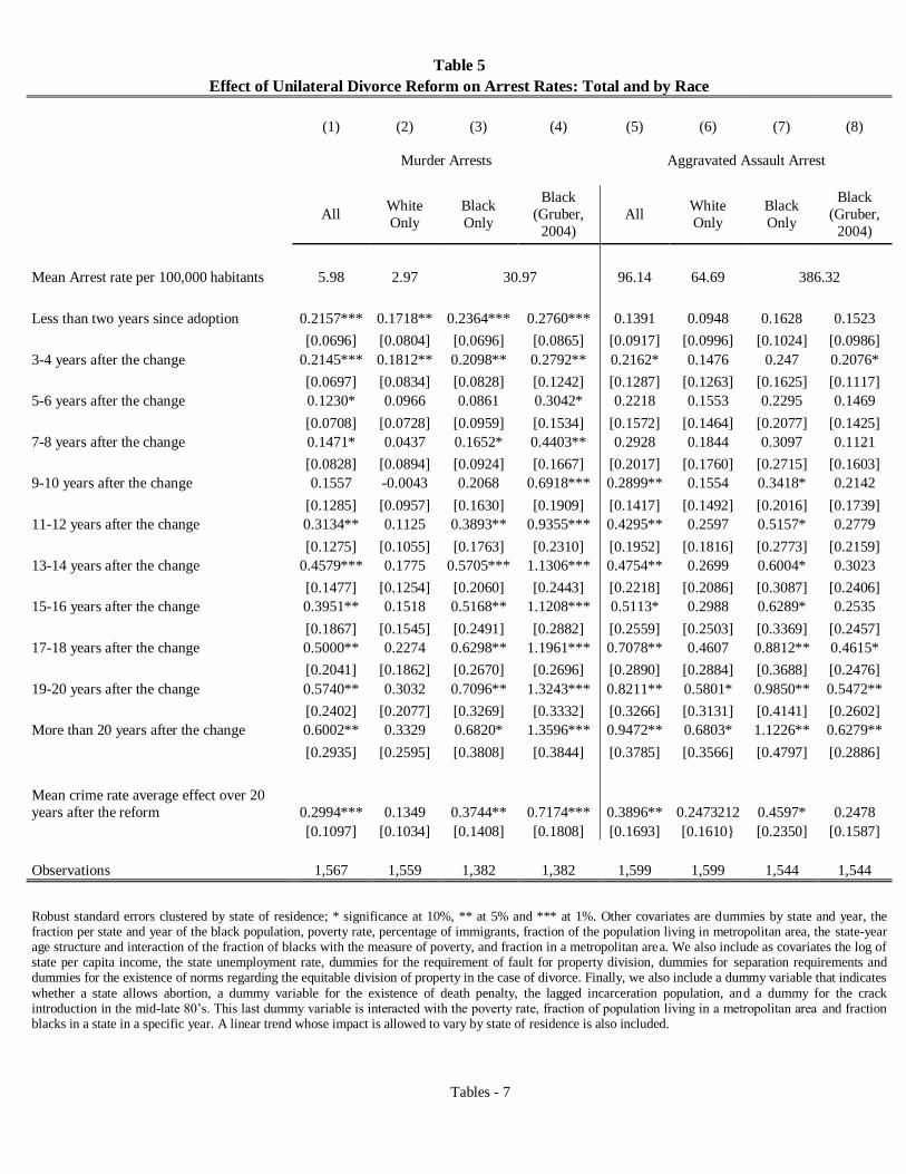
Tables - 7

Table 5

Effect of Unilateral Divorce Reform on Arrest Rates: Total and by Race

(1) (2) (3) (4) (5) (6) (7) (8)

Murder Arrests Aggravated Assault Arrest

All

White

Only

Black

Only

Black

(Gruber,

2004)

All White

Only

Black

Only

Black

(Gruber,

2004)

Mean Arrest rate per 100,000 habitants 5.98 2.97 30.97 96.14 64.69 386.32

Less than two years since adoption 0.2157*** 0.1718** 0.2364*** 0.2760*** 0.1391 0.0948 0.1628 0.1523

[0.0696] [0.0804] [0.0696] [0.0865] [0.0917] [0.0996] [0.1024] [0.0986]

3-4 years after the change 0.2145*** 0.1812** 0.2098** 0.2792** 0.2162* 0.1476 0.247 0.2076*

[0.0697] [0.0834] [0.0828] [0.1242] [0.1287] [0.1263] [0.1625] [0.1117]

5-6 years after the change 0.1230* 0.0966 0.0861 0.3042* 0.2218 0.1553 0.2295 0.1469

[0.0708] [0.0728] [0.0959] [0.1534] [0.1572] [0.1464] [0.2077] [0.1425]

7-8 years after the change 0.1471* 0.0437 0.1652* 0.4403** 0.2928 0.1844 0.3097 0.1121

[0.0828] [0.0894] [0.0924] [0.1667] [0.2017] [0.1760] [0.2715] [0.1603]

9-10 years after the change 0.1557 -0.0043 0.2068 0.6918*** 0.2899** 0.1554 0.3418* 0.2142

[0.1285] [0.0957] [0.1630] [0.1909] [0.1417] [0.1492] [0.2016] [0.1739]

11-12 years after the change 0.3134** 0.1125 0.3893** 0.9355*** 0.4295** 0.2597 0.5157* 0.2779

[0.1275] [0.1055] [0.1763] [0.2310] [0.1952] [0.1816] [0.2773] [0.2159]

13-14 years after the change 0.4579*** 0.1775 0.5705*** 1.1306*** 0.4754** 0.2699 0.6004* 0.3023

[0.1477] [0.1254] [0.2060] [0.2443] [0.2218] [0.2086] [0.3087] [0.2406]

15-16 years after the change 0.3951** 0.1518 0.5168** 1.1208*** 0.5113* 0.2988 0.6289* 0.2535

[0.1867] [0.1545] [0.2491] [0.2882] [0.2559] [0.2503] [0.3369] [0.2457]

17-18 years after the change 0.5000** 0.2274 0.6298** 1.1961*** 0.7078** 0.4607 0.8812** 0.4615*

[0.2041] [0.1862] [0.2670] [0.2696] [0.2890] [0.2884] [0.3688] [0.2476]

19-20 years after the change 0.5740** 0.3032 0.7096** 1.3243*** 0.8211** 0.5801* 0.9850** 0.5472**

[0.2402] [0.2077] [0.3269] [0.3332] [0.3266] [0.3131] [0.4141] [0.2602]

More than 20 years after the change 0.6002** 0.3329 0.6820* 1.3596*** 0.9472** 0.6803* 1.1226** 0.6279**

[0.2935] [0.2595] [0.3808] [0.3844] [0.3785] [0.3566] [0.4797] [0.2886]

Mean crime rate average effect over 20

years after the reform 0.2994*** 0.1349 0.3744** 0.7174*** 0.3896** 0.2473212 0.4597* 0.2478

[0.1097] [0.1034] [0.1408] [0.1808] [0.1693] [0.1610} [0.2350] [0.1587]

Observations 1,567 1,559 1,382 1,382 1,599 1,599 1,544 1,544

Robust standard errors clustered by state of residence; * significance at 10%, ** at 5% and *** at 1%. Other covariates are dummies by state and year, the fraction per state and year of the black population, poverty rate, percentage of immigrants, fraction of the population living in metropolitan area, the state-year age structure and interaction of the fraction of blacks with the measure of poverty, and fraction in a metropolitan area. We also include as covariates the log of state per capita income, the state unemployment rate, dummies for the requirement of fault for property division, dummies for separation requirements and dummies for the existence of norms regarding the equitable division of property in the case of divorce. Finally, we also include a dummy variable that indicates

whether a state allows abortion, a dummy variable for the existence of death penalty, the lagged incarceration population, and a dummy for the crack introduction in the mid-late 80’s. This last dummy variable is interacted with the poverty rate, fraction of population living in a metropolitan area and fraction blacks in a state in a specific year. A linear trend whose impact is allowed to vary by state of residence is also included.

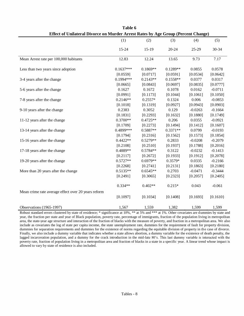
Tables - 8

Table 6

Effect of Unilateral Divorce on Murder Arrest Rates by Age Group (Percent Change)

(1) (2) (3) (4) (5)

15-24 15-19 20-24 25-29 30-34

Mean Arrest rate per 100,000 habitants 12.83 12.24 13.65 9.73 7.17

Less than two years since adoption 0.1637*** 0.1869** 0.1289** 0.0855 0.0578

[0.0559] [0.0717] [0.0591] [0.0534] [0.0642]

3-4 years after the change 0.1994*** 0.2143** 0.1558** 0.0377 0.0317

[0.0665] [0.0843] [0.0697] [0.0835] [0.0777]

5-6 years after the change 0.1627 0.1672 0.1078 0.0162 -0.0711

[0.0991] [0.1173] [0.1044] [0.1061] [0.1050]

7-8 years after the change 0.2146** 0.2557* 0.1324 0.006 -0.0853

[0.1018] [0.1319] [0.0927] [0.0943] [0.0903]

9-10 years after the change 0.2383 0.3052 0.129 -0.0263 -0.1664

[0.1831] [0.2293] [0.1632] [0.1880] [0.1749]

11-12 years after the change 0.3700** 0.4725** 0.206 0.0355 -0.0921

[0.1709] [0.2273] [0.1494] [0.1412] [0.1607]

13-14 years after the change 0.4899*** 0.5887** 0.3371** 0.0799 -0.0193

[0.1794] [0.2316] [0.1562] [0.1573] [0.1854]

15-16 years after the change 0.4422** 0.5279** 0.2833 -0.0208 -0.2079

[0.2108] [0.2510] [0.1937] [0.1788] [0.2016]

17-18 years after the change 0.4889** 0.5784** 0.3122 -0.0232 -0.1413

[0.2117] [0.2672] [0.1933] [0.1912] [0.2078]

19-20 years after the change 0.5727** 0.6979** 0.3579* 0.0335 -0.2166

[0.2268] [0.2741] [0.2131] [0.1863] [0.2180]

More than 20 years after the change 0.5135** 0.6545** 0.2703 -0.0471 -0.3444

[0.2491] [0.3065] [0.2323] [0.2057] [0.2405]

Mean crime rate average effect over 20 years reform

0.334** 0.402** 0.215* 0.043 -0.061

[0.1097] [0.1034] [0.1408] [0.1693] [0.1610}

Observations (1965-1997) 1,567 1,559 1,382 1,599 1,599

Robust standard errors clustered by state of residence; * significance at 10%, ** at 5% and *** at 1%. Other covariates are dummies by state and

year, the fraction per state and year of Black population, poverty rate, percentage of immigrants, fraction of the population living in metropolitan area, the state-year age structure and interaction of the fraction of blacks with the measure of poverty, and fraction in a metropolitan area. We also include as covariates the log of state per capita income, the state unemployment rate, dummies for the requirement of fault for property division, dummies for separation requirements and dummies for the existence of norms regarding the equitable division of property in the case of divorce. Finally, we also include a dummy variable that indicates whether a state allows abortion, a dummy variable for the existence of death penalty, the lagged incarceration population, and a dummy for the crack introduction in the mid-late 80’s. This last dummy variable is interacted with the poverty rate, fraction of population living in a metropolitan area and fraction of blacks in a state in a specific year. A linear trend whose impact is allowed to vary by state of residence is also included.

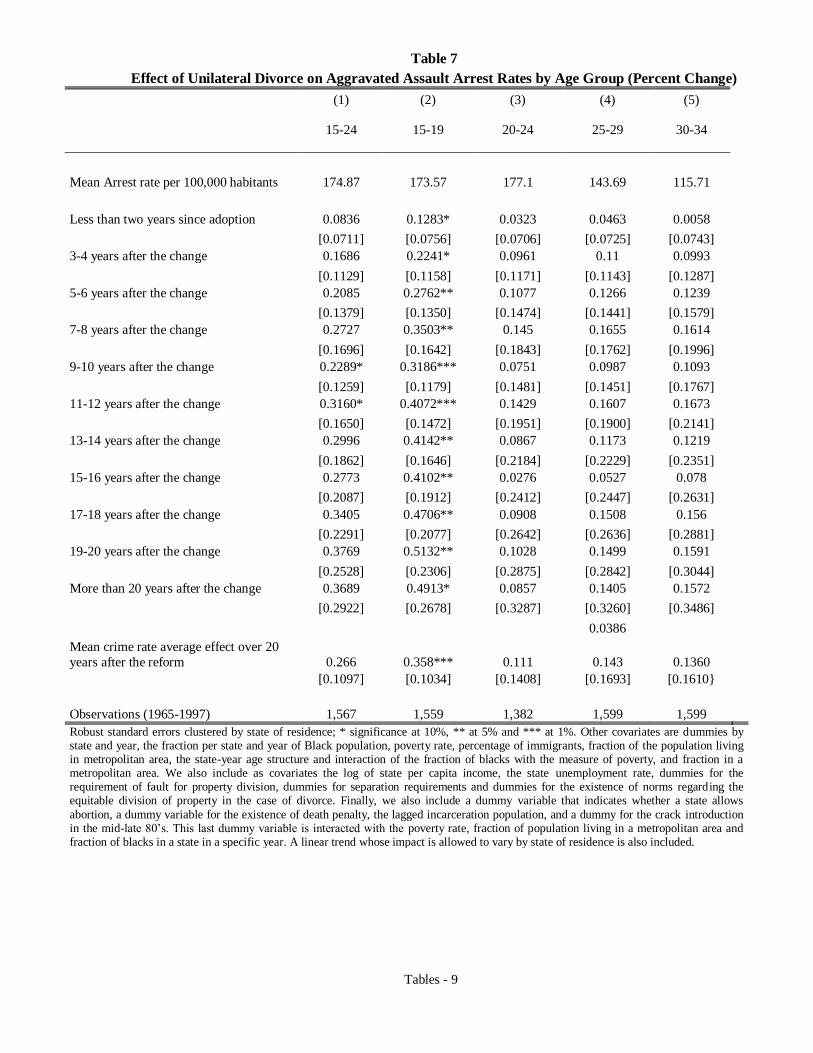
Tables - 9

Table 7

Effect of Unilateral Divorce on Aggravated Assault Arrest Rates by Age Group (Percent Change)

(1) (2) (3) (4) (5)

15-24 15-19 20-24 25-29 30-34

Mean Arrest rate per 100,000 habitants 174.87 173.57 177.1 143.69 115.71

Less than two years since adoption 0.0836 0.1283* 0.0323 0.0463 0.0058

[0.0711] [0.0756] [0.0706] [0.0725] [0.0743]

3-4 years after the change 0.1686 0.2241* 0.0961 0.11 0.0993

[0.1129] [0.1158] [0.1171] [0.1143] [0.1287]

5-6 years after the change 0.2085 0.2762** 0.1077 0.1266 0.1239

[0.1379] [0.1350] [0.1474] [0.1441] [0.1579]

7-8 years after the change 0.2727 0.3503** 0.145 0.1655 0.1614

[0.1696] [0.1642] [0.1843] [0.1762] [0.1996]

9-10 years after the change 0.2289* 0.3186*** 0.0751 0.0987 0.1093

[0.1259] [0.1179] [0.1481] [0.1451] [0.1767]

11-12 years after the change 0.3160* 0.4072*** 0.1429 0.1607 0.1673

[0.1650] [0.1472] [0.1951] [0.1900] [0.2141]

13-14 years after the change 0.2996 0.4142** 0.0867 0.1173 0.1219

[0.1862] [0.1646] [0.2184] [0.2229] [0.2351]

15-16 years after the change 0.2773 0.4102** 0.0276 0.0527 0.078

[0.2087] [0.1912] [0.2412] [0.2447] [0.2631]

17-18 years after the change 0.3405 0.4706** 0.0908 0.1508 0.156

[0.2291] [0.2077] [0.2642] [0.2636] [0.2881]

19-20 years after the change 0.3769 0.5132** 0.1028 0.1499 0.1591

[0.2528] [0.2306] [0.2875] [0.2842] [0.3044]

More than 20 years after the change 0.3689 0.4913* 0.0857 0.1405 0.1572

[0.2922] [0.2678] [0.3287] [0.3260] [0.3486]

0.0386

Mean crime rate average effect over 20

years after the reform 0.266 0.358*** 0.111 0.143 0.1360

[0.1097] [0.1034] [0.1408] [0.1693] [0.1610}

Observations (1965-1997) 1,567 1,559 1,382 1,599 1,599

Robust standard errors clustered by state of residence; * significance at 10%, ** at 5% and *** at 1%. Other covariates are dummies by state and year, the fraction per state and year of Black population, poverty rate, percentage of immigrants, fraction of the population living in metropolitan area, the state-year age structure and interaction of the fraction of blacks with the measure of poverty, and fraction in a metropolitan area. We also include as covariates the log of state per capita income, the state unemployment rate, dummies for the requirement of fault for property division, dummies for separation requirements and dummies for the existence of norms regarding the equitable division of property in the case of divorce. Finally, we also include a dummy variable that indicates whether a state allows

abortion, a dummy variable for the existence of death penalty, the lagged incarceration population, and a dummy for the crack introduction in the mid-late 80’s. This last dummy variable is interacted with the poverty rate, fraction of population living in a metropolitan area and fraction of blacks in a state in a specific year. A linear trend whose impact is allowed to vary by state of residence is also included.

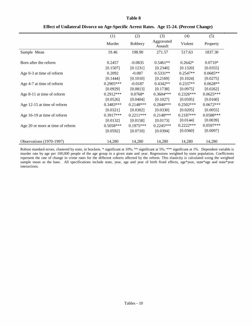
Tables - 10

Table 8

Effect of Unilateral Divorce on Age-Specific Arrest Rates. Age 15-24. (Percent Change)

(1) (2) (3) (4) (5)

Murder Robbery

Aggravated

Assault Violent Property

Sample Mean 19.46 198.90 271.57 517.63 1837.30

Born after the reform 0.2457 -0.0835 0.5461** 0.2642* 0.0710*

[0.1507] [0.1231] [0.2340] [0.1320] [0.0355]

Age 0-3 at time of reform 0.2092 -0.087 0.5331** 0.2547** 0.0685**

[0.1444] [0.1010] [0.2169] [0.1024] [0.0275]

Age 4-7 at time of reform 0.2905*** -0.0187 0.4342** 0.2337** 0.0628**

[0.0929] [0.0813] [0.1738] [0.0975] [0.0262]

Age 8-11 at time of reform 0.2912*** 0.0768* 0.3604*** 0.2326*** 0.0625***

[0.0526] [0.0404] [0.1027] [0.0595] [0.0160]

Age 12-15 at time of reform 0.3483*** 0.2148*** 0.2840*** 0.2502*** 0.0672***

[0.0321] [0.0302] [0.0330] [0.0205] [0.0055]

Age 16-19 at time of reform 0.3917*** 0.2211*** 0.2148*** 0.2187*** 0.0588***

[0.0132] [0.0158] [0.0173] [0.0144] [0.0039]

Age 20 or more at time of reform 0.5058*** 0.1975*** 0.2245*** 0.2222*** 0.0597***

[0.0592] [0.0710] [0.0394] [0.0360] [0.0097]

Observations (1970-1997) 14,280 14,280 14,280 14,280 14,280

Robust standard errors, clustered by state, in brackets. * significant at 10%; ** significant at 5%; *** significant at 1%. Dependent variable is murder rate by age per 100,000 people of the age group in a given state and year. Regressions weighted by state population. Coefficients represent the rate of change in crime rates for the different cohorts affected by the reform. This elasticity is calculated using the weighted sample mean as the base. All specifications include state, year, age and year of birth fixed effects, age*year, state*age and state*year

interactions.

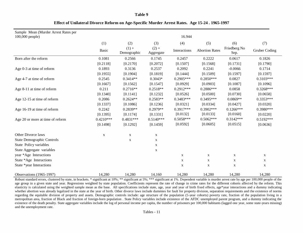
Tables - 11

Table 9

Effect of Unilateral Divorce Reform on Age-Specific Murder Arrest Rates. Age 15-24 . 1965-1997

Sample Mean (Murder Arrest Rates per

100,000 people) 16.944

(1) (2) (3) (4) (5) (6) (7)

Basic

(1) +

Demographic

(2) +

Aggregate Interactions Abortion Rates

Friedberg No

Sep. Gruber Coding

Born after the reform 0.1081 0.2566 0.1745 0.2457 0.2222 0.0617 0.1826

[0.2118] [0.2170] [0.2072] [0.1507] [0.1568] [0.1731] [0.1790]

Age 0-3 at time of reform 0.1893 0.3136 0.2537 0.2092 0.2241 -0.0066 0.1714

[0.1955] [0.1904] [0.1819] [0.1444] [0.1509] [0.1597] [0.1597]

Age 4-7 at time of reform 0.2545 0.3414** 0.3043* 0.2905*** 0.2850*** 0.0827 0.3103***

[0.1667] [0.1562] [0.1547] [0.0929] [0.0903] [0.1087] [0.1096]

Age 8-11 at time of reform 0.211 0.2716** 0.2518** 0.2912*** 0.2886*** 0.0858 0.3268***

[0.1340] [0.1141] [0.1232] [0.0526] [0.0500] [0.0730] [0.0658]

Age 12-15 at time of reform 0.2086 0.2624** 0.2583** 0.3483*** 0.3495*** 0.0869** 0.3353***

[0.1337] [0.1086] [0.1236] [0.0321] [0.0334] [0.0427] [0.0320]

Age 16-19 at time of reform 0.2242 0.2839** 0.2979** 0.3917*** 0.3902*** 0.1266*** 0.3980***

[0.1395] [0.1174] [0.1331] [0.0132] [0.0133] [0.0160] [0.0220]

Age 20 or more at time of reform 0.4210*** 0.4831*** 0.5140*** 0.5058*** 0.5062*** 0.3142*** 0.5192***

[0.1498] [0.1292] [0.1459] [0.0592] [0.0605] [0.0515] [0.0636]

Other Divorce laws x x x

State Demographic Controls x x

State Policy variables x

State Aggregate variables x

year *Age Interactions x x x x

State *Age Interactions x x x x

State *year Interactions x x x x

Observations (1965-1997) 14,280 14,280 14,160 14,280 14,280 14,280 14,280

Robust standard errors, clustered by state, in brackets. * significant at 10%; ** significant at 5%; *** significant at 1%. Dependent variable is murder arrest rate by age per 100,000 people of the age group in a given state and year. Regressions weighted by state population. Coefficients represent the rate of change in crime rates for the different cohorts affected by the reform. This elasticity is calculated using the weighted sample mean as the base. All specifications include state, age, year and year of birth fixed effects, age*year interactions and a dummy indicating whether abortion was already legalized in the state at the year of birth. Other divorce laws include dummies for fault for property division, separation requirements and the existence of norms regarding the equitable division of property and assets. Demographic controls include: age structure of the population (5-year cohorts) poverty rate, fraction of the population living in a metropolitan area, fraction of Black and fraction of foreign-born population . State Policy variables include existence of the AFDC unemployed parent program, and a dummy indicating the existence of the death penalty. State aggregate variables include the log of personal income per capita, the number of prisoners per 100,000 habitants (lagged one year, some state-years missing) and the unemployment rate.

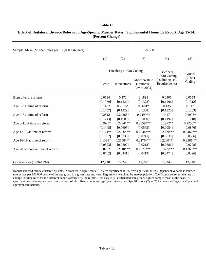
Tables - 12

Table 10

Effect of Unilateral Divorce Reform on Age-Specific Murder Rates. Supplemental Homicide Report. Age 15-24.

(Percent Change)

Sample Mean (Murder Rates per 100,000 habitants) 25.560

(1) (2) (3) (4) (5)

Friedberg (1998) Coding Friedberg

(1998) Coding

(excluding sep.

Requirements)

Gruber

(2004)

Coding

Basic Interactions

Abortion Rate

(Donohue-

Levitt, 2004)

Born after the reform 0.0124 0.172 0.1898 0.0906 0.0558

[0.1959] [0.1224] [0.1322] [0.1296] [0.1312]

Age 0-3 at time of reform 0.1482 0.2316* 0.2601* 0.135 0.112

[0.1737] [0.1229] [0.1308] [0.1320] [0.1383]

Age 4-7 at time of reform 0.2512 0.2426** 0.2499** 0.17 0.1905*

[0.1743] [0.1009] [0.1000] [0.1197] [0.1118]

Age 8-11 at time of reform 0.2625* 0.2294*** 0.2359*** 0.1972** 0.2258**

[0.1448] [0.0605] [0.0593] [0.0954] [0.0876]

Age 12-15 at time of reform 0.2121** 0.2266*** 0.2344*** 0.2389*** 0.2462***

[0.1052] [0.0235] [0.0241] [0.0630] [0.0556]

Age 16-19 at time of reform 0.1398* 0.2158*** 0.2176*** 0.2260*** 0.2581***

[0.0823] [0.0207] [0.0213] [0.0381] [0.0278]

Age 20 or more at time of reform 0.0732 0.2010*** 0.1977*** 0.1635*** 0.1260***

[0.0702] [0.0441] [0.0419] [0.0474] [0.0326]

Observations (1976-1999) 12,240 12,240 12,240 12,240 12,240

Robust standard errors, clustered by state, in brackets. * significant at 10%; ** significant at 5%; *** significant at 1%. Dependent variable is murder rate by age per 100,000 people of the age group in a given state and year. Regressions weighted by state population. Coefficients represent the rate of change in crime rates for the different cohorts affected by the reform. This elasticity is calculated using the weighted sample mean as the base. All specifications include state, year, age and year of birth fixed effects and age*year interactions. Specifications (2) to (5) include state*age, state*year and age*year interactions.