Working Paper Series

7/2012

The Impact of Volatility on Economic Growth

Aurelijus Dabušinskas, Dmitry Kulikov, Martti Randveer

The Working Paper is available on the Eesti Pank web site at:www.bankofestonia.ee/pub/en/dokumendid/publikatsioonid/seeriad/uuringud/

For information about subscription call: +372 668 0998; Fax: +372 668 0954e-mail: publications@eestipank.ee

ISBN 978-9949-493-10-4Eesti Pank. Working Paper Series, ISSN 1406-7161; 7

The Impact of Volatility on Economic Growth

Aurelijus Dabušinskas * , Dmitry Kulikov and Martti Randveer **

Abstract

This paper investigates the impact of macroeconomic volatility on

growth in a panel of 121 countries over the period 1980 to 2010. We

confirm the Ramey and Ramey (1995) result that macroeconomic

volatility is negatively related to economic growth using a different

empirical methodology and a newer dataset. Among the issues that

await further work are the interaction of financial development and

volatility, potential non-linearities of the impact of macroeconomic

volatility on growth, and issues related to the endogeneity of growth

and volatility in the context of empirical growth regression models.

JEL Code: E40, O40, C33

Keywords: economic growth, macroeconomic volatility, growth regressions,

panel data

Corresponding author’s e-mail address: dmitry.kulikov@eestipank.ee

The views expressed are those of the authors and do not necessarily represent

the official views of Eesti Pank.

* Aurelijus Dabušinskas is the Head of the Economics and Research Department, Bank of

Lithuania, Lithuania. **

Bank of Estonia, Estonia.

The authors would like to thank Liina Kulu for research assistance. The authors also wish to

thank conference participants of the 71st International Atlantic Economic Conference in

Athens and the 3rd

International Conference „Economies of Central and Eastern Europe:

Convergence, Opportunities and Challenges“ in Tallinn for their helpful comments and

suggestions. All remaining errors and omissions are our own.

2

Non-technical summary

The aim of the paper is to assess the impact of volatility on economic de-

velopment. More specifically, we focus on macroeconomic volatility and its

potential cost in terms of lower economic growth. We think of volatility as

fluctuations in the growth rate, and distinguish between realised volatility,

commonly measured by standard deviation of actual output growth, and inno-

vation volatility, which is proxied for example by standard deviation of “un-

expected” or unpredicted growth.

An oft-cited paper that galvanised the issue by demonstrating the presence

of a statistically and economically significant negative relationship between

volatility and growth was Ramey and Ramey (1995). Their data covered 92

countries for the period of 1962–1985; the dependent variable was per capita

output growth, and volatility was measured as either realised or innovation

variability in output growth. Ramey and Ramey estimation results implied

that an increase in realised volatility of one standard deviation was associated

with lower per capita growth of over half a percentage point in the whole

sample of countries and with lower growth of about one-third of a percentage

point in OECD countries.

This paper investigates the impact of macroeconomic volatility on growth

in a panel of 121 countries over the period 1980 to 2010. We confirm the

Ramey and Ramey (1995) result that macroeconomic volatility is negatively

related to economic growth using a different empirical methodology and a

newer dataset. We make a distinction between several sub-groups of coun-

tries, such as high-income OECD member countries, a group of Eastern Eu-

ropean countries, high-growth Asian economies, and others.

Our preliminary estimates suggest that for the full sample of 121 coun-

tries, a 50-percent increase in volatility translates into 0.4-percentage-point

lower annual per capita growth. The analogous estimate based on the sub-

sample of OECD countries is about 10 percent smaller but is statistically in-

distinguishable from the whole-sample result. A similar result applies for the

group of Eastern European countries, which includes the three Baltic coun-

tries.

Among the issues that await further work are the interaction of financial

development and volatility, potential non-linearities of the impact of macro-

economic volatility on growth, and issues related to the endogeneity of

growth and volatility in the context of empirical growth regression models.

3

Contents

1. Introduction .................................................................................................. 4

2. Data and econometric methodology ............................................................. 8

3. Empirical results ......................................................................................... 11

4. Conclusions ................................................................................................ 14

References ...................................................................................................... 15

Appendix A: Data sources .............................................................................. 16

4

1. Introduction

The aim of the paper is to assess the impact of volatility on economic de-

velopment. More specifically, we focus on macroeconomic volatility and its

potential cost in terms of lower economic growth. In empirical contexts, we

will think of volatility as fluctuations in the growth rate, in which case it is

useful to distinguish between realised volatility, commonly measured by

standard deviation of actual output growth, and innovation volatility, proxied,

for example, by standard deviation of ‘unexpected’ or unpredicted growth.1

Theoretical models, in contrast, typically capture such uncertainty more fun-

damentally by standard deviations of structural shocks such as productivity or

demand. Our focus on the link between volatility and growth is of course

only one way of thinking about the consequences or costs of volatility; the

choice seems justified, however, given how central economic growth is for

welfare in the longer run.

In the realm of mainstream economics, the question of how volatility af-

fects economic growth is relatively new. Prior to the emergence of the real

business cycle (RBC) theory, economic growth and business cycle fluctu-

ations were regarded as two separate issues, in, for example, the Solow

growth model and the IS-LM framework. It was believed that the two phe-

nomena had different causes and that, consequently, long-term economic

growth was independent of cyclical factors. Other approaches, like the

Schumpeterian paradigm of creative destruction and the Austrian school,2

were in this sense more integrated but were not mainstream and thus were far

less influential.

With the birth of RBC theory in the early 1980s (Kydland and Prescott

(1982)), cyclical fluctuations and economic growth begin to be analysed in a

unified modelling framework, but the previous dichotomy remains. As be-

fore, it is presumed that economic growth is driven by permanent incremental

improvements in productivity through technological progress, and even

though the RBC explanation that higher frequency fluctuations are caused by

temporary productivity shocks is novel, the variability of these disturbances –

the extent of cyclical volatility – is believed to have only second order effects

on growth. One important implication of this view was shown by Lucas

(1987): in an RBC world, the welfare costs of business cycle fluctuations,

and thus the benefit of eliminating them, amount to only 0.06 percent of

steady state consumption. Many felt the estimate was too low, but the result

1 This distinction is very clear in Ramey and Ramey (1995).

2 In a nutshell: monetary policy mistakes like being too accommodating in upswings

foster credit booms, which, in turn, lead to over-investment and eventual busts.

5

was partly due to the assumption that temporary cyclical fluctuations have no

first-order implications for long-term growth.

An oft-cited paper that galvanised the issue by demonstrating the presence

of a statistically and economically significant negative relationship between

volatility and growth was Ramey and Ramey (1995). Their data covered 92

countries for the period 1962–1985; the dependent variable was per capita

output growth, and volatility was measured as either realised or innovation

variability in output growth. The Ramey and Ramey estimation results im-

plied that an increase in realised volatility of one standard deviation was as-

sociated with lower per capita growth of over half a percentage point in the

whole sample of countries and with lower growth of about one-third of a per-

centage point in OECD countries (see Table 1 in Appendix). Importantly, this

negative relationship was robust to controlling for the investment-to-GDP

ratio, which meant that volatility was reducing growth not, or not only, by

lowering investments but via some other mechanism(s) as well. More recent

re-estimations of the Ramey and Ramey equations using updated data series

(Aghion and Banerjee (2005)) confirm these results, though the negative

volatility coefficient is no longer statistically significant for the OECD sub-

sample (see the last two columns of Table 1 in Appendix).

It would seem natural to seek theoretical grounds for the negative relation-

ship between volatility and growth in endogenous growth models. However,

as Aghion and Banerjee (2005) explain succinctly, the two main conceptual

mechanisms of endogenous growth ― the AK model and the Schumpeterian

paradigm ― tend to suggest that volatility should affect growth positively

rather than negatively. To reconcile the theoretical implications with this em-

pirical evidence, Aghion and Banerjee (2005) argue it is necessary to modify

these models by introducing an additional crucial feature of economic reality

― imperfections in the functioning of financial markets.

In the AK framework,3 the impact of volatility on economic growth is am-

biguous because it depends on two counteracting effects. On the one hand,

higher volatility leads to higher saving, due to precautionary motives, re-

sulting in higher investment and thus faster growth. On the other, it reduces

risk-adjusted returns, which lowers investment as well as growth. The net

effect depends on the elasticity of inter-temporal substitution, which is

usually also equal to the coefficient of relative risk aversion, and particularly

on whether it is bigger or smaller than unity. Though there is substantial un-

certainty about the true magnitude of this elasticity, Aghion and Banerjee

3 The engine of growth in the AK model is capital accumulation, and the key element

guaranteeing that this growth is everlasting is the assumption that at the aggregate level capi-

tal is not subject to diminishing returns. It is common to assume that the aggregate produc-

tion function is linear in aggregate capital, hence the acronym AK.

6

argue that most empirical estimates for it fall in the range where the precau-

tionary motive dominates, and the implied volatility-growth relationship is

positive.

To illustrate the Schumpeterian paradigm of endogenous growth, Aghion

and Banerjee assume that firms face two types of investment: capital invest-

ments that are always productive in the short run and longer-term invest-

ments that are subject to uncertainty but have the potential to generate im-

provements in technology through innovations. The crux of this set-up is that

long-term growth becomes directly dependent on the intensity of innovative

(R&D) investment in the economy. Importantly for our discussion, this mod-

el implies that R&D investments and thus long-term growth are countercycli-

cal and that, by implication, volatility is good for growth. The main reason

for this outcome is the opportunity cost effect: in recessions, when short-term

projects are less profitable, it is relatively cheaper to invest for the long term.

In this way, economic slumps become fertile grounds for the kinds of invest-

ment that deliver future technological advancements, the driver of long-term

growth.

Since the prediction of a positive relationship between volatility and

growth lacks empirical support, Aghion and Banerjee argue that a key miss-

ing element in these growth models is financial frictions, because in the real

world, firms are financially constrained, and financial markets are imperfect.

To demonstrate the implications that such frictions have for the Schum-

peterian growth model, they introduce an additional assumption that longer-

term productivity-enhancing investments are subject to interim financing re-

quirements which are initially uncertain. Firms can meet these financing

needs by drawing on their own cash flow or by borrowing, but the maximum

amount that lenders are willing to lend in each case is assumed to be a fixed

multiple of the financial wealth available to the firm.

If sufficiently binding, such financial constraints reverse the counter-cycli-

cality of longer-term innovative investments because firms’ cash flows and

their ability to borrow to satisfy interim liquidity needs worsen during reces-

sions. That also changes the volatility-growth relationship from positive to

negative: volatility creates uncertainty in firms’ liquidity positions, and that

discourages them from making productivity-enhancing investments. This

characterisation is accurate not only for the extreme cases of financing con-

straints: if financial frictions are above a certain very-high level, innovative

investments are forgone and the economy stays on a low-growth path; con-

versely, if financing is relatively frictionless and collateral requirements are

below a certain level, productivity-enhancing investments are made and the

economy grows rapidly. For intermediate levels of financing frictions, the

model implies a monotonic negative relationship between volatility and

growth.

7

In this stylised framework, the extent to which financial constraints are

binding is controlled by the model parameter determining the maximum

amount of credit that can be extended for a given level of financial wealth as

collateral. In the real world, that should correlate with the level of financial

sector development, as more advanced financial intermediation makes bor-

rowing against future cash flows easier. The model predicts, then, that the

negative effect of macroeconomic volatility on growth should be weaker in

countries with more developed financial sectors.

According to Aghion and Banerjee (2005), this hypothesis is supported by

the data. First they use cross-sectional growth regressions similar to those in

Ramey and Ramey (1995) but modified to include the private sector credit-

to-GDP ratio as a proxy for the depth of financial intermediation and an inter-

action of this ratio with the volatility measure to confirm that the negative

volatility-growth association is weaker (less negative) when the credit ratio is

higher. Moreover they show the estimated financial sector effect is substan-

tial: it is strong enough to make the overall impact of volatility on growth

positive for the countries that have the most financially advanced financial

sectors. Second, similar estimations using panel data show that the terms of

trade and commodity price shocks ― two examples of exogenous causes of

volatility ― have a lower impact on growth in countries with more developed

financial sectors, again measured by the credit-to-GDP ratio.

Today, the idea that volatility and economic growth correlate negatively is

quite widely accepted.4 Easterly et al. (2000), for example, take it as given

and raise an important follow up question: if macroeconomic volatility is bad

for growth, what causes it? In particular, Easterly et al. (2000) argue that,

when trying to explain output volatility, macroeconomists have put too much

emphasis on price and wage rigidities and labour market flexibility, and paid

too little attention to the crucial role of the financial sector and financial fac-

tors in general.5 Using panel data for a large cross-section of countries, they

indeed obtain no statistically significant link between their measure of real

wage flexibility (standard deviation of real wage growth) and volatility in

growth. Importantly however, they find that the private credit to GDP ratio, a

proxy for financial sector development, is related to volatility in a non-linear

4 In a recent paper, Benigno et al. (2010) argue that macroeconomic volatility may in-

crease long-term unemployment. A central theoretical mechanism that implies this result in

their model is asymmetric (stronger downwards) real wage rigidity. As the realisation of

strongly adverse productivity shocks becomes more likely when the variability of productiv-

ity shocks is high, firms are more reluctant to hire if lowering real wages in bad times is dif-

ficult. As a consequence, higher macroeconomic volatility leads to higher long-term unem-

ployment. Benigno et al. (2010) show that this mechanism is important for explaining

unemployment trends in the US data. 5 Financial institutions, cash flow constraints, firm wealth effects and other balance

sheet effects, etc.

8

way: while the credit to GDP ratio remains below a certain level, the finan-

cial sector plays a stabilising role, but as it gets deeper and more sophisti-

cated its association with volatility becomes positive. Instead of diversifying

and insuring risks, very advanced financial sectors may in fact create addi-

tional risks. In the circumstances of the recent crisis, many would find this

argument particularly relevant and appealing today.6

As mentioned earlier, in this paper we will estimate the impact of vola-

tility on economic growth. The earlier empirical estimates are based on data

from until 2000 and therefore do not include the latest data from before the

global financial crisis and the data from during the financial crisis, which

might change the earlier conclusions. Although it is not included in this ver-

sion of the paper, we plan an estimate of the impact of the interaction be-

tween financial constraints and volatility on economic growth and an assess-

ment of whether the impact of volatility on economic growth is non-linear.

The paper is structured as follows. In Section 2 we present the methodol-

ogy and data. In Section 3 we discuss the main empirical results. Section 4

concludes.

2. Data and econometric methodology

This section details the data collection and processing strategy used in the

paper. It also provides an overview of the econometric methodology behind

the empirical growth-volatility regressions in Section 3.

The empirical part of this paper uses a wide sample of countries, drawing

most of the time series from the IMF’s International Financial Statistics data-

base.7 The full sample period covers the last three decades, from 1980 to

2010. Inevitably, some of the countries are dropped out of the sample be-

cause of missing data. Out of 144 countries in the IMF’s International Finan-

cial Statistics database, 23 countries are completely excluded from the sam-

ple due to their inadequate data coverage. For many of the remaining coun-

tries, the available data series start later than 1980, sometimes spanning just

the last ten years of the full sample period. However, since this does not pre-

sent a problem from the modelling point of view, the countries with partial

data coverage are still included in the empirical growth-volatility regressions

6 Easterly et al. (2000) also find that volatility is typically higher in developing countries

and countries more open to international trade. Concerning the latter they note, however, that

openness is also known to contribute to growth itself, so the overall effect is likely to be

positive. 7 See http://www.imfstatistics.org/IMF .

9

in Section 3 of this paper. The full sample of countries used in the empirical

part of this paper is listed in Table 2 of the Appendix.

For each country in the sample the following annual data series are col-

lected from the IMF’s International Financial Statistics database: (i) real GPD

per capita in PPP terms, (ii) nominal GDP, (iii) nominal gross fixed capital

formation outlays, (iv) nominal government consumption expenditure, (v)

nominal exports of goods and services, and (vi) population in millions. In

addition, the average years of schooling over five-year periods for each coun-

try in the sample are obtained from the World Bank’s EdStats database.8

The following data processing strategy is used to compile the set of vari-

ables used in the growth-volatility regressions in Section 3 of this paper. The

full 30-year sample period is divided into six equal five-year sub-periods,

starting with the first sub-period spanning the years 1980 to 1984, and ending

with the last sub-period from 2005 to 2010. For each of the countries in the

sample, indexed by i, and each of the six sub-periods, indexed by t, the fol-

lowing variables are computed: (i) ity∆ is the average annual growth rate of

real GPD per capita in PPP terms over the corresponding sub-period in per-

centage points; (ii) itσ is the standard deviation of the average annual growth

rate of real GPD per capita in PPP terms over the corresponding sub-period;

(iii) ity is the average annual real GPD per capita in PPP terms over the cor-

responding sub-period; (iv) itn∆ is the average annual population growth rate

over the corresponding sub-period; (v) its is the average years of schooling

over the corresponding sub-period; (vi) iti is the average annual investment

share in GDP over the corresponding sub-period, calculated as the ratio of

nominal gross fixed capital formation outlays to nominal GDP; (vii) itg is

the average annual government consumption share in GDP over the corre-

sponding sub-period, calculated as the ratio of nominal government con-

sumption expenditures to nominal GDP; and (viii) ite is the average annual

export share in GDP over the corresponding sub-period, calculated as the

ratio of nominal exports of goods and services to nominal GDP. This data

compilation strategy effectively creates a panel data set, with a cross-

sectional dimension indexed by individual countries in the sample, and a time

dimension given by six five-year sub-periods, over which the averages of the

relevant country-specific macroeconomic indicators are computed.

The choice of econometric methodology in this paper is guided by several

considerations. The growth-volatility regressions in Section 3 of this paper

can be regarded as empirical models designed for measuring the impact of

macroeconomic volatility on economic growth in a wide sample of heteroge-

8 See http://data.worldbank.org/data-catalog .

10

neous countries over the last three decades. They are vaguely related to

growth theory, but cannot be treated as structural econometric relationships

between a well-defined set of variables with well-understood structural pa-

rameters. Therefore, this paper emphasises simplicity, flexibility and robust-

ness in its statistical assessment of the impact of volatility on growth. At the

same time, given the complexity of this research question and the restrictions

imposed by the limited sample scope, the issues of endogeneity and omitted

variables loom large. Clearly, these two econometric issues need to be given

proper attention if the empirical implications of the growth-volatility regres-

sions in Section 3 are to be considered plausible.

This paper adopts the following linear regression view of the possible em-

pirical link between economic growth and macroeconomic volatility in a

panel of countries:

ittiititit uacXy ++++=∆ − δβσγ 1log (1)

In this linear regression model the primary parameter of interest that links

macroeconomic volatility to economic growth is γ . The log transform of itσ

is adopted for empirical reasons, as itσ is non-negative by construction with

a lot of statistical information concentrated in a small neighbourhood around

zero, whereas the distribution of itσlog is evened out across the real line.

The set of controls in 1−itX consists of 1log −ity , 1−∆ itn , 1−its , 1−iti , 1−itg , 1−ite ,

and an intercept. All variables in 1−itX pre-date the period over which the real

per capita GDP growth ity∆ and the corresponding volatility itσ are mea-

sured.9 This mitigates the potential endogeneity issues in model (1), which, if

present, may spill over to the estimate of γ , as well as fitting nicely into the

overall framework of the empirical growth theory. In order to address the

issue of sample heterogeneity and omitted variables, a set of individual

country fixed effects ic is added to the model, taking care of such potentially

important factors as geography, climate, natural resources, time-invariant po-

litical effects, and so on. The impact of time-varying factors affecting eco-

nomic growth on the global scale over the last three decades, such as changes

in world-wide trade, energy prices, or the economic and political climate, is

taken care of by a set of time dummies ta . Finally, the idiosyncratic compo-

nent of the economic growth in this panel of countries is assumed to come

from a white noise term itu .

The parameters of this linear regression are estimated by the fixed effects

estimator (see Wooldridge (2010)). It should be recalled that the fixed effects

9 Note that this specification implies that out of six five-year sub-periods available in the

full panel dataset, only five sub-periods are actually used for the purpose of statistical infer-

ence.

11

estimator does not impose any assumptions on the dependence between ic

and the remaining set of explanatory variables. This is particularly important

for the sample heterogeneity and omitted variables issue in an empirical in-

vestigation of growth-volatility linkages. A comparison to the bare-bones

pooled OLS results is also proved, where the latter omits the country-specific

fixed effects ic .

3. Empirical results

Before going into the discussion of empirical growth-volatility regres-

sions, it is instructive to take a closer look at the simple unconditional corre-

lation of macroeconomic growth and volatility in the sample of 121 countries

over the period of three decades from 1980 to 2010. Table 2 in the Appendix

lists the corresponding sample statistics: ity∆ and itσ are simple arithmetic

averages of, respectively, ity∆ -s and itσ -s over iT five-year sub-periods, for

which the corresponding variables are available for each particular country.

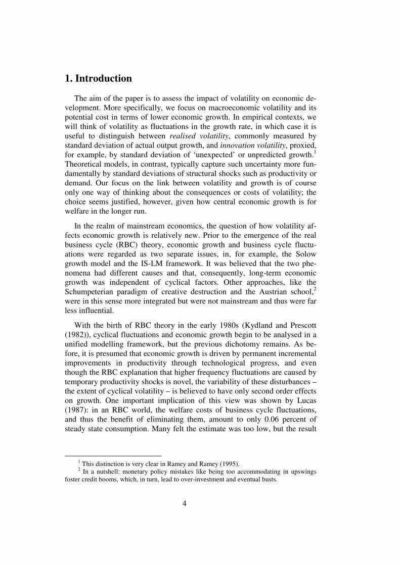
Their cross plot is displayed on Figure 1, and their unconditional correlation

is equal to 0.0127. A weak negative correlation of –0.0343 between ity∆ and

itσ is obtained when Armenia is excluded from the sample, but in any case

the unconditional correlation between macroeconomic growth and volatility

in the sample remains extremely weak. This finding is broadly in line with

the corresponding empirical evidence in the literature (see Ramey and Ramey

(1995)), once again highlighting a substantial heterogeneity across the sample

countries.

The empirical growth-volatility regressions are summarised in Table 1,

where both the pooled OLS and panel fixed effects estimates of the main pa-

rameters are listed. In addition to the reported results, time-dummy param-

eters δ and a time-invariant intercept are also estimated, but their estimates

are not reported in the table. The total number of observations used for the

statistical inference is 540, and they are split across 121 countries and five

time periods, as described in Section 2. In addition, a smaller sub-sample of

155 observations from the 33 countries which were OECD members at the

end of 2010 is also used for comparative purposes.

12

Figure 1: Cross plot of the average macroeconomic growth and its standard

deviation in the sample of 121 countries over the period 1980 to 2010

Note: Country abbreviations follow the ISO 3166 standard (see Table 2 in the Appendix A).

In line with Ramey and Ramey (1995) and many others, the empirical re-

sults in Table 1 point to a negative contemporaneous link between macroeco-

nomic volatility and growth in the sample of 121 countries over the last three

decades. The negative link is statistically significant across both the pooled

OLS and the panel fixed effects versions of the model, getting even stronger

in the latter case, when the sample heterogeneity is accounted for by the

country-specific fixed effects.

Of the six remaining control variables, only the preceding period log in-

come level 1log −ity and population growth rate 1−∆ itn retain their statistical

significance across the pooled OLS and panel fixed effects versions of the

model. Both of them also have the expected negative partial effect on growth,

along the lines of Ramey and Ramey (1995) and Levine and Renelt (1992).

Note that the effects of these two controls on ity∆ differ noticeably across the

two sets of estimates in Table 1, implying that the unaccounted for country-

specific heterogeneity in the pooled OLS version of the model can lead to

some sizeable and potentially important distortions.

ALDZ

AR

AM

AU

AT

BH

BD

BBBE

BZ

BJBO

BW

BRBN

BG

BI

KH

CMCA

CF

CL

CO

CGCR

CI

HR

CY

CZ

DK

DOEC

EG

SV

EE

FJ

FI

FR

GA

GM DE

GH

GRGT

GY

HN

HK

HU

IS

IN

ID

IR

IE

IL

IT

JM JP

JO

KZ

KE

KR

KG

LV

LS

LY

LT

LU

MW

MY

ML

MT

MR

MU

MXMN

MA

MZ

NA

NPNL

NZ

NE

NOPK

PA

PG

PY

PE

PH

PLPT

QA

RORU

RW

SA

SN

RS

SK

SI

ZAES

LK

SZSECH

TZ

TH

TG

TN

TR

UG

UA

GBUS

UY

VE

VNYE

ZM

02

46

8V

ola

tilit

y

0 2 4 6 8 10Growth

13

Table 1: Empirical growth-volatility regressions

Independent variable Pooled OLS

Full sample

Fixed effects

Full sample

Fixed effects

OECD sample

Log volatility ( itσlog ) –0.7051** –0.9286** –0.8590**

(-4.62) (–6.14) (–3.40)

Log income level ( 1log −ity ) –0.7305** –7.8478** –9.6451**

(-5.30) (–9.85) (–6.52)

Population growth rate

( 1−∆ itn ) –0.6156** –0.3891** –0.8146*

(–6.74) (–3.09) (–1.84)

Education level ( 1−its ) 0.1785** –0.1722 –0.0970

(2.86) (–0.93) (–0.51)

Investment share ( 1−iti ) 0.0350** 0.0124 –0.0223

(2.07) (0.40) (–0.45)

Government consumption

share ( 1−itg ) –0.0276 0.0136 –0.0990

(–1.40) (0.36) (–1.62)

Export share ( 1−ite ) 0.0154** 0.0070 0.0344**

(3.47) (0.58) (2.08) 2

R 0.25 0.45 0.68

No of observations 540 540 155

Notes: Pooled OLS and fixed effects estimation results for model (1) are shown in the table.

Full sample consists of 121 countries listed in Table 2 of the Appendix. OECD sample is the

33 countries which were OECD members at the end of 2010. Estimates of the time dummies

and a time-invariant intercept are not shown. Numbers in parentheses are robust t-statistics.

The superscripts ** and * indicate that the corresponding coefficient is statistically signifi-

cant at the 5% and 10% confidence level respectively. For the fixed effects estimator, 2

R

refers to the within statistic

Having said that, the previous period partial effects of education level

1−its , investment share 1−iti , government consumption share 1−itg , and export

share 1−ite on the economic growth in the following period ity∆ in the pooled

OLS version of the model in Table 1 all have empirically plausible signs.

In a smaller sample of 33 OECD countries, the fixed effects estimator un-

covers a very similar picture of the negative partial effect of volatility on

growth, with the corresponding coefficient being statistically indistinguish-

able from its full sample counterpart. In addition, the growth-volatility re-

gression for the OECD countries has a statistically significant positive effect

on openness to world trade, as measured by the export share 1−ite , on eco-

nomic growth in the next period.

14

The overall fit of the estimated growth-volatility models in Table 1 is

measured by the reported 2R statistics, and points to a substantial remaining

heterogeneity still unaccounted for by the three empirical models.

4. Conclusions

Using more recent data and a broader sample of countries, we confirm

the Ramey and Ramey (1995) result that macroeconomic volatility is neg-

atively related to economic growth. Our estimates for the whole sample of

121 countries indicate that a 50-percent increase in volatility translates into

0.4-percentage-point lower annual per capita growth. The analogous estimate

based on the sub-sample of OECD countries is about 10 percent smaller but

statistically indistinguishable from the whole-sample result.

The similarity of our findings for a broad set of countries and the OECD

sub-sample contrasts with the empirical evidence discussed by Aghion and

Banerjee (2005) who argue that the negative volatility-growth relationship is

harder to detect in OECD countries. According to Aghion and Banerjee, such

a tendency can be explained by their theoretical model, in which the more de-

veloped financial sectors of the OECD countries can reduce the financial fric-

tions which make volatility detrimental to growth. A recent paper by Arcand,

Berkes and Panizza (2012) examines non-linear effects of financial depth,

measured as the fraction of private credit to GDP, on medium-term economic

growth in a panel of 133 countries over the time periood 1960 to 2010. In

contrast to Aghion and Banerjee (2005), empirical results reported by

Arcand, Berkes and Panizza (2012) confirm that macroeconomic volatility

still retains its negative and statistically significant effect on medium-term

growth even in the presence of controls for the financial sector size.

We intend to address the interaction of financial development and

volatility and the potential non-linearities in their effects on economic growth

in a future version of this paper.

15

References

AGHION, P., G. ANGELETOS, A. BANEJEE AND K. MANOVA (2005):

“Volatility and growth: credit constraints and productivity-enhancing

investment”, NBER Working Paper, No. 11349.

AGHION, P. AND A. BANERJEE (2005): “Volatility and growth”, Oxford

University Press.

ARCAND, J.L., E. BERKES AND U. PANIZZA (2012): „Too Much

Finance?“ IMF Working Paper, WP/12/161.

BENIGNO, P., L.A. RICCI AND P. SURICO (2010): “Unemployment and

productivity in the long run: the role of macroeconomic volatility”,

NBER Working Paper, No. 16374.

EASTERLY, W., R. ISLAM AND J.E. STIGLITZ (2000): “Shaken and

stirred: explaining growth volatility”. In Pleskovic B. and N. Stern

(eds.). Annual World Bank Conference on Development Economics,

The World Bank, Washington, D.C., 191–211.

KYDLAND, F. AND E. PRESCOTT (1982): “Time to build and aggregate

fluctuations”, Econometrica, 1982, No. 50(6), 1345–1370.

LEVINE, R. AND D. RENELT (1992): “A sensitivity analysis of cross-

country growth regressions”, American Economic Review, No. 82(4),

942–963.

LUCAS, R.E., Jr (1987): Models of business cycles, Blackwell, Oxford.

LUCAS, R.E., Jr. (2003): “Macroeconomic Priorities”, American Economic

Review, No. 93(1), 1–14.

RAMEY, G. AND V.A. RAMEY (1995): “Cross-country evidence on the

link between volatility and growth”, American Economic Review, No.

85(5), 1138–1151.

WOOLDRIDGE, J.F. (2010): Econometric analysis of cross section and

panel data. The MIT Press, 2nd

edition.

16

Appendix A: Data sources Table 1: Relationship between average growth and volatility

Ramey and Ramey (1995) AABM (2004)a

Sample All countries

1962–1985

OECD

1952–1988

All countries

1960–1995

OECD

1960–1995

Effect of

volatilityb

–0.21*** –0.39* –0.22** –0.29

Summary of variance estimates (all variance figures are multiplied by 1,000)

Mean variance

(st.dev.)

3.58 (0.06) 0.99 (0.03)

Lowest variance

(st.dev.)

0.317 (0.018)

(Swed)

0.299 (0.017)

(Nor)

Highest variance

(st.dev.)

28.7 (0.17)

(Iraq)

2.90 (0.054)

(Tur)

US variance

(st.dev.)

0.663 (0.026) 0.596 (0.024)

Notes: a Aghion, Angeletos, Banerjee and Manova (2004) as reported in Aghion and Banerjee

(2005).

b Ramey and Ramey (1995): controlling for average investment share, average population

growth, initial human capital, initial per capita GDP; AABM (2004): controlling for average

investment share, average population growth, secondary school enrolment, initial per capita

GDP, government size, inflation, black market premium, trade openness, intellectual

property rights, property rights.

17

Table 2: Average economic growth and its standard deviation by country

Country ity∆ itσ iT Country ity∆ itσ iT

Albania (AL) 7.13 2.27 2 Korea Republic

(KR) 7.88 3.26 5

Algeria (DZ) 2.81 2.21 5 Kyrgyz Republic

(KG) 5.05 4.17 3

Argentina (AR) 3.94 6.06 3 Latvia (LV) 7.10 5.92 3

Armenia (AM) 10.07 5.62 3 Lesotho (LS) 4.19 2.87 5

Australia (AU) 4.32 1.20 5 Libya (LY) 1.07 7.45 5

Austria (AT) 4.12 1.80 5 Lithuania (LT) 7.22 6.00 3

Bahrain (BH) 3.24 5.19 5 Luxembourg (LU) 5.88 3.23 5

Bangladesh (BD) 5.31 0.84 5 Malawi (MW) 3.09 5.17 5

Barbados (BB) 3.32 2.10 4 Malaysia (MY) 5.54 4.30 5

Belgium (BE) 4.15 1.95 5 Mali (ML) 4.41 3.98 5

Belize (BZ) 5.80 4.65 5 Malta (MT) 4.92 2.32 5

Benin (BJ) 3.25 2.01 5 Mauritania (MR) 3.49 3.45 4

Bolivia (BO) 3.33 1.98 5 Mauritius (MU) 6.74 2.32 5

Botswana (BW) 6.40 4.04 5 Mexico (MX) 3.23 3.80 5

Brazil (BR) 3.27 2.72 4 Mongolia (MN) 5.66 3.55 3

Brunei Darussalam

(BN) 0.23 2.63 1 Morocco (MA) 4.64 4.51 5

Bulgaria (BG) 5.02 4.21 3 Mozambique (MZ) 6.71 3.77 5

Burundi (BI) 1.70 3.71 5 Namibia (NA) 4.25 2.54 3

Cambodia (KH) 6.42 4.29 4 Nepal (NP) 4.84 1.80 5

Cameroon (CM) 1.01 2.12 5 Netherlands (NL) 4.33 1.92 5

Canada (CA) 3.84 1.91 5 New Zealand (NZ) 3.42 1.78 5

Central African

Republic (CF) 0.95 3.71 4 Niger (NE) 2.20 4.56 5

Chile (CL) 6.10 3.08 5 Norway (NO) 4.39 1.76 5

Colombia (CO) 4.36 2.01 5 Pakistan (PK) 4.60 1.99 5

Congo Republic (CG) 3.56 4.94 5 Panama (PA) 4.79 4.03 5

Costa Rica (CR) 5.11 4.75 1 Papua New Guinea

(PG) 2.95 4.61 5

Côte d'Ivoire (CI) 1.24 1.85 5 Paraguay (PY) 2.76 3.32 5

Croatia (HR) 5.57 3.74 3 Peru (PE) 3.80 5.47 5

Cyprus (CY) 5.18 2.89 5 Philippines (PH) 3.60 3.13 5

Czech Republic (CZ) 5.37 3.38 2 Poland (PL) 5.51 2.56 5

Denmark (DK) 3.81 2.14 5 Portugal (PT) 4.80 2.39 5

Dominican Republic

(DO) 5.00 3.53 5 Qatar (QA) 2.06 8.74 5

Ecuador (EC) 3.58 3.68 5 Romania (RO) 3.31 4.97 5

Egypt Arab Republic

(EG) 4.74 1.30 5

Russian Federation

(RU) 5.49 5.10 3

El Salvador (SV) 4.10 2.09 3 Rwanda (RW) 3.48 7.16 5

Estonia (EE) 7.35 5.71 3 Saudi Arabia (SA) 1.98 3.54 5

Fiji (FJ) 3.69 4.34 5 Senegal (SN) 2.95 1.98 5

Finland (FI) 4.21 2.84 5 Serbia (RS) 6.56 4.94 1

France (FR) 3.80 1.69 5 Slovak Republic

(SK) 6.19 3.50 3

Gabon (GA) 1.73 5.44 5 Slovenia (SI) 5.10 2.87 3

Gambia (GM) 2.86 2.02 2 South Africa (ZA) 3.01 2.29 5

18

Germany (DE) 3.94 1.95 5 Spain (ES) 4.64 2.03 5

Ghana (GH) 4.32 1.10 4 Sri Lanka (LK) 5.88 1.87 5

Greece (GR) 4.30 2.09 5 Swaziland (SZ) 5.04 2.26 5

Guatemala (GT) 2.75 1.95 5 Sweden (SE) 3.96 2.05 5

Guyana (GY) 4.03 3.57 4 Switzerland (CH) 3.34 1.96 5

Honduras (HN) 3.39 2.70 5 Tanzania (TZ) 4.52 1.53 5

Hong Kong (HK) 5.73 3.80 5 Thailand (TH) 6.56 4.10 5

Hungary (HU) 3.90 2.89 5 Togo (TG) 1.65 5.31 5

Iceland (IS) 4.04 3.34 5 Tunisia (TN) 5.16 2.31 5

India (IN) 6.56 2.16 5 Turkey (TR) 4.56 6.05 4

Indonesia (ID) 5.61 3.16 5 Uganda (UG) 4.99 3.92 5

Iran Islamic Republic

(IR) 3.67 5.60 5 Ukraine (UA) 3.80 6.33 3

Ireland (IE) 6.00 3.13 5 United Kingdom

(GB) 4.36 1.61 5

Israel (IL) 4.42 2.73 5 United States (US) 4.06 1.48 5

Italy (IT) 3.59 1.80 5 Uruguay (UY) 5.07 3.69 5

Jamaica (JM) 2.99 2.67 5 Venezuela (VE) 2.90 6.71 5

Japan (JP) 4.05 2.63 5 Vietnam (VN) 7.77 1.73 3

Jordan (JO) 2.88 3.89 5 Yemen Republic

(YE) 2.67 1.61 3

Kazakhstan (KZ) 7.24 3.59 3 Zambia (ZM) 1.98 3.58 5

Kenya (KE) 3.00 1.98 5

Notes:

Listed above are the average economic growth ity∆ and its standard deviation itσ over the

sample period 1980 to 2010 for each country. The corresponding sample means across all

countries are 4.33 for ity∆ and 3.33 for itσ . The number of five-year sub-periods, for which

the variables in model (1) are available for each particular country, is shown in the iT

column.

Working Papers of Eesti Pank 2012

No 1Kadri MännasooDeterminants of Bank Interest Spread in Estonia

No 2Jaanika MeriküllHouseholds borrowing during a creditless recovery

No 3Merike Kukk, Dmitry Kulikov, Karsten StaehrConsumption Sensitivities in Estonia: Income Shocks of Different Persistence

No 4David SeimJob Displacement and Labor Market Outcomes by Skill Level

No 5Hubert Gabrisch, Karsten StaehrThe Euro Plus Pact: Competitiveness and External Capital Flows in the EU Countries

No 6Aleksei NetšunajevReaction to Technology Shocks in Markov-switching Structural VARs: Identification via Heteroskedasticity