1

The Implicit Prices of Finfish and Shellfish Attributes and Retail Promotion

Strategies: Hedonic Analysis of Weekly Scanner Data in the U.S.

Dr. Sherry Larkin

Glen Gold

University of Florida

slarkin@ufl.edu glengold@ufl.edu

Selected Paper prepared for presentation at the Southern Agricultural Economics

Association Annual Meeting, Birmingham, AL, February 4-7, 2012.

Copyright 2012 by Dr. Sherry Larkin and Glen Gold. All rights reserved. Readers may make

verbatim copies of this document for non-commercial purposes by any means, provided that this

copyright notice appears on all such copies.

2

Abstract

Using AC Neilson retail scanner data on U.S. frozen finfish and shellfish sales from 2007-2010,

hedonic models of each market estimated price discounts following the Deepwater Horizon oil

spill and as a result of promotional activities, and premiums and discounts for select products

labeled “wild” and “imported”, respectively.

Introduction

The US seafood industry is composed of a plethora of heterogeneous products. Much research

and analysis has been performed to understand what drives sales and prices of various products

within this industry. We know from past research that consumers place value on a variety of

seafood attributes and qualities (Roheim, Gardiner, and Asche, 2007; McConnell and Strand,

2000). Attributes that have been shown to affect price include product quality (McConnell and

Strand, 2000), form, brand, species, size and processing (Roheim, Gardiner, and Asche, 2007).

Leek and Maddock (2000) study the “situational determinants” that may encourage consumers’

choice to buy.

The objective of this paper is to expand on these commonly accepted factors by

introducing promotional, labeling and situational variables to a hedonic model of seafood prices.

This study hypothesizes that P=f(X,Y), where X is a vector of promotional, labeling and

situational variables and Y is a vector of product attributes.

At its simplest division, the seafood industry is composed of finfish and shellfish. This

study will estimate pricing models for both markets which provide a base to make comparisons

between the shellfish and finfish markets in the United States. The shellfish market (not

including shrimp), with an average weekly revenue of 40% that of the finfish market, serves as

3

an appropriate comparison group providing both similarities and differences in product,

promotional labeling and situational attributes (A.C. Neilson). Albeit less average weekly

revenue than finfish, the shellfish market obtains 40% the revenue with approximately one third

the average weekly volume sold (in packages) (A.C. Neilson).

Attributes of most interest in this study are the following: promotional effects on pricing,

seasonality effects of Christmas and Lent holidays, impacts of the Deepwater Horizon Gulf Oil

Spill, and the effect of labeling products as “imported” or “wild”.

The effect of labeling products as wild is of particular interest due to the recent push

towards the development and implementation of eco-labeling programs within the seafood

industry. With both governments and consumer groups pressuring the industry to act in a more

sustainable way, an understanding of the price effects these popular labels have on seafood could

be used to help justify industry standards and/or policy decisions. Research by Roheim, Asche

and Santos (2011) recently calculated the marginal increase of a consumers’ willingness to pay

for MSC-certified frozen processed Alaska Pollock in the London metropolitan area in the UK

market.

The most common method of learning consumers’ preferences toward fish has been

through conjoint analysis (Anderson and Brooks, 1986; Sylvia and Larkin, 1994). Using hedonic

analysis, implicit prices of various product attributes can be calculated (McConnell and Strand,

2000). Due to the availability of retail scanner data, more recent studies have been able to use

hedonic analysis to calculate the revealed preferences of consumers (Roheim, Gardiner, and

Asche, 2007). This study of the US finfish and shellfish market will serve as a platform for

which other more focused research studies may follow.

4

The Hedonic Model

The basis of the hedonic model is the assumption that a product is composed of a variety of

specific attributes or characteristics that the consumer values independently. Generally, first

degree hedonic models ignore production and demand effects on a goods’ price, however,

changes in production and demand may be picked up through the use of seasonal attributes (such

as increased sunscreen sales in hotter months) in a hedonic model.

The hedonic model estimates the shadow (or implicit) price of each individual attribute.

The total price of a product is calculated as the sum of the shadow prices of each attribute. In this

study, retail scanner data supplies the market prices of the various unbreaded frozen fish and

shellfish goods examined in this study.

The model results are used to identify the statistically significant variables and the sign

and magnitude of the associated parameter estimates. A negative parameter estimate indicates

that the attribute lowered the overall price of the good in the market and time periods covered.

Conversely, a positive parameter estimate for a specific attribute indicates that the attribute

increased the overall price of a good. Ultimately, consumer preferences as observed in the retail

market are extracted for various product characteristics.

Data

Retail scanner data for all frozen unbreaded fish and shellfish (“unbreaded remaining”) products

were obtained from AC Neilson. The focus on unbreaded products was designed to capture those

that the producer may have more control over. Unbreaded products, in general, have less

processing performed than their breaded counterparts and perhaps fewer middlemen between the

harvester and consumer.

5

To reduce the amount of noise in the data, products that did not sell for at least 1/3 of the

time frame are removed from the data set. This method was previously applied by Roheim,

Gardiner, and Asche (2007). Some species not typically considered seafood were also removed,

such as frogs

The data contains weekly sales of an individual products (as defined by UPC code)

aggregated from grocery stores with at least 2 million dollars in annual sales, and that are located

within metro areas of the United States. The data begins with the week ending June 17, 2007 and

ends with the week ending June 12, 2010. Each observation contains qualitative variables on

UPC, brand, product (i.e., species), form, size description and type; and quantitative variables on

week, year, rank, size, dollars (i.e., sales), units (i.e., packages), promotional dollars, and

promotional units. For a sale to qualify as promotional, it must either be made during a time of

advertisement, with or without a price adjustment; or sold at an adjusted price without

advertisement.

Total Dollars is the weekly revenue of each product. It is calculated by taking the sum of

promotional dollars and non-promotional dollars. The average weekly revenue for shellfish is

$4,074 and $9,572 for finfish. The maximum total weekly revenue for shellfish is $374,152 and

$991,375 for finfish. The maximum non-promotional dollars is about half the maximum

promotional dollars in both markets. Average weekly revenues are also examined by “proportion

of promotional sales” groups. This will be expanded on later.

Total Package is a measurement of product volume. It is calculated by taking the sum of

promotional packages and non-promotional packages sold during a given week. The average

weekly packages sold are 638 for shellfish and 1,800 for finfish. The weekly maximum non-

6

promotional packages sold was about one fourth the weekly maximum promotional packages

sold for both markets.

Through calculations made with dollars, units, promotional dollars, promotional units and

size variables, the dependent variable “adjusted weighted price per pound” was calculated. Price

was weighted by the proportion of sales made under promotion. The price per pound is adjusted

for inflation using the Consumer Price Index, base 2007. The dependent variable has a mean

value of $9.09 for shellfish and $5.17 for finfish. The maximum adjusted weighted price per

pound was $86 for shellfish and $148 for finfish. This relatively high values are associated with

specialty products in small (i.e., <= 10 ounce packages).

The proportion of sales made under promotion variable, PROP, is a continuous number

between 0 and 1. It is calculated using packages sold, to determine the proportion of sales made

under promotion for each weekly observation. For example, this variable does not pick up

proportions between products sold fully promotional one week of the month, and fully non-

promotional the remaining three weeks. The PROP variable can then be assigned to one of four

PROP groups: PROP = 0, PROP < 0.5, PROP ≥ 0.5 and PROP = 1. Observations which fall into

the middle groups are considered to be strategically promoted because the products are only

promoted in certain cities or stores, and not promoted everywhere else, during that week.

Observations which fall into the PROP = 0 or PROP = 1 group are either not promoted or fully

promoted across the entire U.S. market during that week. Products that are strategically

promoted with more promotional than non-promotional sales fall into the group PROP ≥0.5. This

group has the highest average total dollars for shellfish and finfish, $11,873 and $24,817,

respectively. The mean of the PROP variable indicates that 17% of the shellfish and 22% of the

finfish observation were sold under promotion.

7

Three time event variables were specified (OS, LENT, and CMAS) in order to capture

sales made during the weeks following the Deepwater Horizon Oil Spill, two weeks in February

(capturing the onset of the Lent season and Valentines’ Day sales collectively), and the two

weeks prior to Christmas, respectively. Each of these variables in each model (finfish and

shellfish) accounted for 3% to 5% of the observations.

The brand variable, NameBrand identifies products that were sold under a private label

versus under the stores’ label. Approximately 90% of shellfish and 81% of finish were sold

under private labels.

The special attribute category, Labeling, reveals information pertaining to location of

catch, whether the product was imported, and some product form information that was species-

specific. The finfish market has a higher percentage of products that do not have any additional

special attributes (50%) than the shellfish market (25%). In terms of special labels, 36% of the

shellfish market was comprised of imported products. Unfortunately, this label is not included on

any of the finfish products. However, over 7% of the finfish market over the period covered was

comprised of products that were labeled as “wild”.

The size variable, Size, has a mean of 21 ounces for both shellfish and finfish. It is

notable, given the previously mentioned finding that smaller packages occasionally were

associated with relatively high prices on a per pound basis, that 16% of the shellfish market and

14% of the finfish market was composed of products with a package size less of than or equal to

10 oz. An examination of the outliers, from a statistical basis (i.e., products with an adjusted

weighted price per pound outside two standard deviations from the mean), revealed that these

products cost more than $19.47/lb and $26.39/lb for finfish and shellfish, respectively. In the

8

finfish and shellfish markets these outlier products comprise 92% and 85%, respectively, of the

products that are less than or equal to 10 ounces.

The species grouping variables are limited to the inclusion of groupings that account for

at least 1% of the market. Many of the species with less than 1% market share are accounted for

as a subgroup within a more dominant species group.

Estimation and Model Specification

Hedonic regression analysis is used to calculate the implicit prices of several product,

promotional and labeling attributes. Separate models were estimated for finfish and shellfish

since the data sets contained different variables. For example, in the shellfish model, the “type”

variable contains information that identifies a product as imported. This variable does not contain

this information in the finfish model, so combining these data would make the assumption that

all finfish were domestically produced. This would be an incorrect assumption.

Initially, regression analysis is performed in SAS using the PROC REG procedure. Both

heteroscedasticity and autocorrelation are identified as issues with Ordinary Least Squares (OLS)

regression. The HETERO statement is applied to correct for Heteroscedasticity by assuming it is

related to the package size variable. According to Sayrs (1989), heteroscedasticity must be

corrected for prior to the detection of autocorrelation. An assumption of the OLS regression is

that the variances remain consistent across all values of a variable. This is not true along the

values of the size variable due to inconsistencies in product (species) size offerings as well as

increased variability in smaller package sizes. For example, the most common package size has

high “adjusted weighted price per pound” variability because many different products are offered

at that size package.

9

The time variables week and year are used to assign dummy variables to seasonal trends

determined by calculating PROP means by week. In other words, an examination of the average

PROP per week indicated seasonality related to major U.S. holidays when fish and shellfish

products are more or less likely to be on promotion.

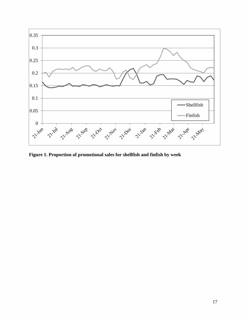
A comparative chart of the 3-year average PROP is particularly interesting (Figure 1). In

the shellfish market, Christmas is the time of heaviest average proportion of promotional

behavior. In the finfish market, Lent is the time of heaviest proportion of promotional behavior.

Shellfish promotion in February peaks prior to finfish, which may be due to promotions

encompassing Valentines’ Day. These peaks are captured with dummy variables to understand

how price is affected during these times of promotional behavior change.

The labeling variables differed between models. The finfish market includes labeling of

“Wild” products as well as regions of harvest. Smoked fish is also a popular type of processing

not present in the shellfish market. The shellfish market does include information pertaining to

the import of particular products. In both models, species-specific product labeling is accounted

for through the use of interaction terms. These interaction terms are necessary account for

particular price differences associated with distinct product (e.g., lobster tails versus crawfish

tails). Labeling variables may be applied to a large number of products (such as wild or regular)

or product specific (such as bay versus sea scallops). Imported shellfish and wild finfish are most

important to this study.

The base product in the finfish model is a whole, name brand Whitefish lacking any

special attribute labeling and not sold under promotion or during any of the “situational

influence” time-periods. The base is the mean package size as well as not sold in a small package

size.

10

The base product in the shellfish model is a whole, name brand Scallop lacking any

special attribute labeling and not sold under promotion or during and of the “situational

influence” time-periods. The base product is the mean for package size as well as not sold in a

small package size.

Results

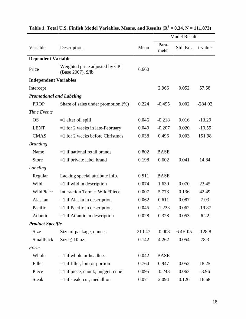
Tables 1 and 2 contain the regression results of the finfish and shellfish models, respectively,

estimated in SAS and corrected for autocorrelation as described previously. The finfish model

used 111,873 observations and had an underlying R2 value of 0.33, and 32 of the 33 variables

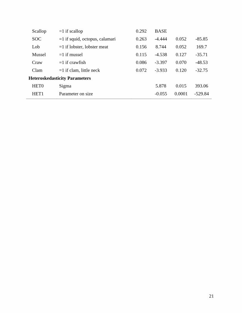
were statistically significant at the 99% level. The shellfish model uses 44,272 observations and

had an underlying R2 of 0.80, and 19 of the 22 variables were statistically significant at the 99%

level of confidence (not including the HET0 and HET1 variables, but note that the latter variable

is statistically significant in both models indicating that heteroskedasticity was present).

The intercept value is larger in the shellfish model than the finfish model, $9.48 and

$2.97, respectively, indicating that the average price of the base shellfish product was over three

times that of finfish, which is to be expected (especially in an unbreaded frozen market). The

magnitude of parameter estimates with respect to the intercept will be reported.

The proportion of promotional sales variable, PROP, has a negative influence in both

models. The magnitude is larger in the shellfish model than the finfish model, 19.8% and 16.7%

respectively.

The oil spill variable, OS, had a negative influence on price in both models. The finfish

market shows an average price cut of $0.22 per pound and the shellfish shows a price cut of

11

$0.33. The magnitude is larger in the finfish model than in the shellfish model, 7.3% and 3.5%

respectively.

LENT had a higher significant parameter estimate in the finfish model than in the

shellfish model. Both estimates are negative. The parameter estimates for the finfish and

shellfish model are -0.21 and -0.14, respectively, and equates to a marginal change of 7% and

1.4% with respect to the intercept.

CMAS had a positive influence in both the finfish and shellfish models. The estimate is

only significant at the 80% level in the shellfish model. The parameter estimates are 0.50 in the

finfish and 0.05 in the shellfish. This equates to a 16.7% and 0.6% marginally higher price.

In the finfish market, labeling products as “wild” had a positive influence on price. The

parameter estimates is 1.64. The magnitude is 55%. The interaction term between wild and piece

is used to distinguish more highly prized pieces of a larger wild fish from less valued smaller

pieces, such as nuggets. A product form of piece labeled as wild has a parameter estimate of

$5.77, which was a 195% increase over the base price.

In the shellfish market, products labeled as imported have a negative influence on price.

The imported parameter estimate is -0.10. This equates to a 1% discount on imported products.

The size variable has a negative influence in both models. The parameter estimates are -

0.0083 and -0.0473 in the finfish and shellfish models, respectively. This equates to a -0.3%

change per ounce of package size in the finfish model and 0.5% change per ounce of package

size in the shellfish model, with respect to the intercept.

The variable to capture products sold in a small package size of less than 10 ounces,

SmallPack, has a positive influence on price in both models. The parameter estimates are 1.90 in

12

the finfish model and 4.26 in the shellfish model. This equates to a marginal change of 144% in

the finfish model and 20% in the shellfish model, with respect to the intercept.

The product form variables are more extensive in the finfish model than the shellfish. As

expected, consumers on average pay more for product forms which are more processed and

contain less waste.

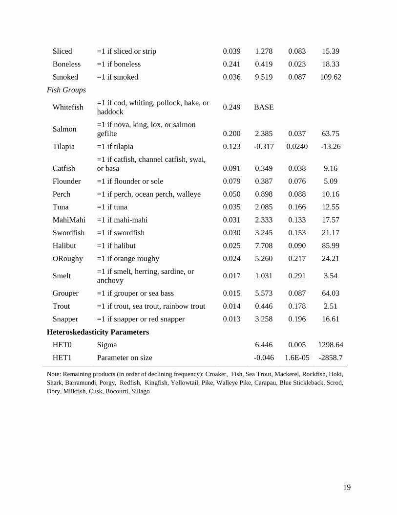
The species groups’ variables are included in the models to correct for price influences

due to the species of the product being sold. Removing the species groups has a dramatic

negative effect on the explanatory power of the models. In the shellfish model, all of the species

group parameter estimates are significant at a 99% level of confidence. With respect to the base

product of Scallop (not labeled as Bay), Lobster is the only parameter estimate with a positive

value. In the finfish model, Trout is the only group not significant at the 99% level (t-value 2.51).

Conclusions

By examining the average revenues by PROP group, it can be determined that promotional

efforts by the finfish and shellfish retailers are successful in increasing the average revenues in

both markets. Highly strategized promotional behavior has the highest weekly average revenue,

with more than half of the products sold being promoted, but not encompassing a “blanket”

promotional strategy for the week. The finfish market is more heavily involved in promotional

behavior than the shellfish market, however, shellfish products sold under promotion are

discounted by a higher margin than finfish, 20% and 17% respectively. Both shellfish and finfish

adjusted weighted price per pound decreases as proportion of promotional sales increases. A

higher percentage of finfish products are sold under promotion than shellfish products. A large

number of products in both markets are “lightly” promoted; this is determined by a PROP mean

13

of 0.19 in the PROP < 0.5 group for both markets. This may be explained by companies testing

specific regional markets in an attempt to identify those which more heavily promotion may be

successful.

The 4% and 7% average decrease in price following the Deepwater Horizon Oil Spill,

may be explained by retailers and producers attempt to increase demand for seafood during a

time in which its safety in question. Some may debate that the oil spill had just started during this

time period, and all the products on the shelf had more than likely been harvested prior to this

disaster. However, such an event acts as a reminder to consumers of past disasters, and revives

past questioning of seafood’s safety. For example, the Exxon Valdez disaster happened more

than 20 years ago, but consumers may begin to question Alaskan seafood once again because

they are reminded of safety concerns due to the new oil spill far from the Alaskan fisheries.

According to a review in the Journal of Environmental Health Perspectives, NOAA initiates the

first fisheries closures on May 2nd

, and expands closures to nearly 84 thousand square miles by

the beginning of July (Gohlke, 2011). This data ends prior to the reopening of closed areas,

which begins on June 23rd

.

The finfish market is more heavily involved in promotions during the Lent season. The

pricing behavior is more clearly estimated in this market than the shellfish. The average marginal

change is much larger, at -7%. This may be explained by the popularity of fish as a substitute for

beef rather than shellfish. This could be further explained by the popularity of shellfish, lobster

in particular, during Valentines’ Day.

Christmas is also a more significant holiday for the finfish market than the shellfish

market with regards to pricing. The finfish market exhibits an average price hike of 17%. This

could be explained by the higher level of promotional sales made during this time for shellfish,

14

and lower level of promotional sales for finfish. Fish is not a popular dinner item during the

Christmas season. The high parameter estimate during Christmas could also be explained by an

increase in the sale of specialty fish products, such as the smoked varieties.

Finfish products labeled as wild demand a price premium in comparison to products not

exhibiting any special attribute information. This evidence could be used to support a movement

by the industry to fully adopt an Eco-Labeling certification program such as the Marine

Stewardship Council (MSC). Although this variable encompasses products not certified, the

results are in line with similar studies done on the value of Eco-Labeled products in the literature

(Roheim, Asche and Santos 2011).

Imported products in the shellfish market are sold at a price discount. The magnitude of

price change is relatively small.

Discussion

These models serve as an overall representation of the United States market for shellfish and

finfish. Specific regional, promotional, labeling and time event models are necessary to reveal

intricacies unable to be detected by these general models. The Simpson Paradox is a

phenomenon which “occurs when a relationship that exists for all subgroups of a population

disappears when the data are aggregated for the whole population” (Klass, 2008). Breaking this

data apart and analyzing specific subgroups of interest could yield more explanatory results.

Recommendations for future studies include:

Improving the calculation of proportion of promotions (PROP) based on a monthly

aggregate of promotional and non-promotional sales. This will allow for the capture of week to

15

week changes in “blanket” promotional and non-promotional strategies which this model does

not capture.

The labeling variables wild and imported could be closer examined. By focusing in on

specific species or regions the explanatory power of the models will be improved. To better

estimate the consumers’ willingness to pay for a wild caught labeling, models of individual

species may be required, as done by Roheim, Asche and Santos (2011). This methodology could

also be applied to estimate the average price discount on products labeled imported. Wild and

imported labeling may also have a higher impact on price in specific regions.

Expand on the holiday variables to better capture or expand on the points of interest in

time. Dummy variables could be assigned to the exact weeks Lent occurs over the three year

period rather than just capturing the onset. Thanksgiving is another trough in the finfish

promotions that could be estimated.

The Oil Spill coefficient can be expanded on and better understood through more current,

encompassing data. This data runs through June 2010, at which point the oil spill was still

flowing and the public concern was continuing to grow. The 3.5% and 7% price discount

determined by this model may very well be a conservative estimate, and data running through the

end of 2010 may reveal more drastic price cuts by retailers to increase demand for seafood

products.

References

Gohlke, J. M., D. Doke, M. Tipre, M. Leader, T. Fitzgerald. “A Review of Seafood Safety after

the Deepwater Horizon Blowout.” Journal of Environmental Health Perspectives

119(2011): 1062-1069.

16

Klass, G. M. Just Plain Data Analysis, Rowman and Littlefield Publishers, Maryland. 2008.

Lambert, J., L. Klieb, and M. Weber. “Regional Influences Upon the Selection of Imported

Versus Domestic Seafood.” Academy of Marketing Studies Journal 12(2008): 17-42.

Leek, S., Maddock, S., Foxall, G. (2000). Situational determinants of Fish Consumption. British

Food Journal, Vol. 102(1). p.18-39.

McConnell, K. E. and I. E. Strand. “Hedonic Prices for Fish: Tuna Prices in Hawaii.” American

Journal of Agricultural Economics 82(2000): 133-144.

Roheim, C. A., F. Asche, and J. I. Santos. “The Elusive Price Premium for Ecolabelled Products:

Evidence from Seafood in the UK Market.” Journal of Agricultural Economics 62(2011):

655-668

Roheim, C. A., L. Gardiner, and F. Asche. “Value of Brands and Other Attributes: Hedonic

Analysis of Retail Frozen Fish in the UK.” Marine Resource Economics 22(2007): 239-

253.

Thrane, M., F. Ziegler, and U. Sonesson. “Eco-labelling of Wild-caught Seafood Products.”

Journal of Cleaner Production 17(2009): 416-423.

Sayrs, L.W. Pooled Time Series Analysis, Sage Publications, California. 1989.

17

Figure 1. Proportion of promotional sales for shellfish and finfish by week

0

0.05

0.1

0.15

0.2

0.25

0.3

0.35

Shellfish

Finfish

18

Table 1. Total U.S. Finfish Model Variables, Means, and Results (R2 = 0.34, N = 111,873)

Model Results

Variable Description Mean Para-

meter Std. Err. t-value

Dependent Variable

Price Weighted price adjusted by CPI

(Base 2007), $/lb 6.660

Independent Variables

Intercept 2.966 0.052 57.58

Promotional and Labeling

PROP Share of sales under promotion (%) 0.224 -0.495 0.002 -284.02

Time Events

OS =1 after oil spill 0.046 -0.218 0.016 -13.29

LENT =1 for 2 weeks in late-February 0.040 -0.207 0.020 -10.55

CMAS =1 for 2 weeks before Christmas 0.038 0.496 0.003 151.98

Branding

Name =1 if national retail brands 0.802 BASE

Store =1 if private label brand 0.198 0.602 0.041 14.84

Labeling

Regular Lacking special attribute info. 0.511 BASE

Wild =1 if wild in description 0.074 1.639 0.070 23.45

WildPiece Interaction Term = Wild*Piece 0.007 5.773 0.136 42.49

Alaskan =1 if Alaska in description 0.062 0.611 0.087 7.03

Pacific =1 if Pacific in description 0.045 -1.233 0.062 -19.87

Atlantic =1 if Atlantic in description 0.028 0.328 0.053 6.22

Product Specific

Size Size of package, ounces 21.047 -0.008 6.4E-05 -128.8

SmallPack Size ≤ 10 oz. 0.142 4.262 0.054 78.3

Form

Whole =1 if whole or headless 0.042 BASE

Fillet =1 if fillet, loin or portion 0.764 0.947 0.052 18.25

Piece =1 if piece, chunk, nugget, cube 0.095 -0.243 0.062 -3.96

Steak =1 if steak, cut, medallion 0.071 2.094 0.126 16.68

19

Note: Remaining products (in order of declining frequency): Croaker, Fish, Sea Trout, Mackerel, Rockfish, Hoki,

Shark, Barramundi, Porgy, Redfish, Kingfish, Yellowtail, Pike, Walleye Pike, Carapau, Blue Stickleback, Scrod,

Dory, Milkfish, Cusk, Bocourti, Sillago.

Sliced =1 if sliced or strip 0.039 1.278 0.083 15.39

Boneless =1 if boneless 0.241 0.419 0.023 18.33

Smoked =1 if smoked 0.036 9.519 0.087 109.62

Fish Groups

Whitefish =1 if cod, whiting, pollock, hake, or

haddock 0.249 BASE

Salmon =1 if nova, king, lox, or salmon

gefilte 0.200 2.385 0.037 63.75

Tilapia =1 if tilapia 0.123 -0.317 0.0240 -13.26

Catfish

=1 if catfish, channel catfish, swai,

or basa 0.091 0.349 0.038 9.16

Flounder =1 if flounder or sole 0.079 0.387 0.076 5.09

Perch =1 if perch, ocean perch, walleye 0.050 0.898 0.088 10.16

Tuna =1 if tuna 0.035 2.085 0.166 12.55

MahiMahi =1 if mahi-mahi 0.031 2.333 0.133 17.57

Swordfish =1 if swordfish 0.030 3.245 0.153 21.17

Halibut =1 if halibut 0.025 7.708 0.090 85.99

ORoughy =1 if orange roughy 0.024 5.260 0.217 24.21

Smelt =1 if smelt, herring, sardine, or

anchovy 0.017 1.031 0.291 3.54

Grouper =1 if grouper or sea bass 0.015 5.573 0.087 64.03

Trout =1 if trout, sea trout, rainbow trout 0.014 0.446 0.178 2.51

Snapper =1 if snapper or red snapper 0.013 3.258 0.196 16.61

Heteroskedasticity Parameters

HET0 Sigma 6.446 0.005 1298.64

HET1 Parameter on size -0.046 1.6E-05 -2858.7

20

Table 2. Total U.S. Shellfish Model Variables, Means, and Results (R2 = 0.80, N = 44,272)

Model Results

Variable Description Mean Para-

meter Std. Err. t-value

Dependent Variable

Price Weighted price adjusted by CPI

(Base 2007), $/lb 8.863

Independent Variables

Intercept 9.483 0.043 221.3

Promotional and Labeling

PROP Share of sales under promotion (%) 0.169 -1.873 0.034 -55.23

Time Events

OS =1 after oil spill 0.042 -0.334 0.066 -5.05

LENT =1 for 2 weeks mid-February 0.040 -0.138 0.052 -2.65

CMAS =1 for 2 weeks before Christmas 0.041 0.053 0.037 1.41

Branding

Name =1 if national retail brands 0.905 BASE

Store =1 if private label brand 0.095 0.398 0.038 10.53

Labeling

Regular Lacking special attribute info. 0.259 BASE

Imported =1 if imported 0.356 -0.102 0.028 -3.71

Atlantic =1 if Atlantic 0.010 3.621 0.029 124.52

Dressed =1 if dressed 0.099 0.596 0.095 6.30

BScallop Interaction term = bay*scallop 0.087 -1.729 0.055 -31.44

CTail Interaction term = crawfish*tail 0.075 -7.294 0.158 -46.31

Product Specific

Size Size of package, ounces 21.019 -0.047 0.0006 -80.51

SmallPack Size ≤ 10 oz. 0.158 1.903 0.051 37.37

Form

Whole =1 if whole or tube 0.573 BASE

Piece =1 if piece, ring, claw, chunk, or cut 0.265 0.123 0.044 2.78

Tail =1 if tail 0.163 11.355 0.063 180.39

Fish Groups

21

Scallop =1 if scallop 0.292 BASE

SOC =1 if squid, octopus, calamari 0.263 -4.444 0.052 -85.85

Lob =1 if lobster, lobster meat 0.156 8.744 0.052 169.7

Mussel =1 if mussel 0.115 -4.538 0.127 -35.71

Craw =1 if crawfish 0.086 -3.397 0.070 -48.53

Clam =1 if clam, little neck 0.072 -3.933 0.120 -32.75

Heteroskedasticity Parameters

HET0 Sigma 5.878 0.015 393.06

HET1 Parameter on size -0.055 0.0001 -529.84