The Importance of Educational Credentials: SchoolingDecisions and Returns in Modern China⇤

Alex EbleBrown University

JOB MARKET PAPER

Feng HuUniversity of Science

and Technology Beijing

January 2016

Abstract

Government policy sets the number of years of schooling needed to attain educationalcredentials such as a high school diploma. We exploit a policy change in China to estimatethe impact of this policy choice on schooling decisions and labor supply. The policy extendedthe length of primary school by one year and was rolled out gradually across China over 25years. We show this has reallocated 850 billion person-hours from labor to schooling to date,as the vast majority of affected individuals chose to earn a credential despite the additionalyear in school this required. A key contribution of our paper is to estimate the returns toan additional year of schooling while holding highest credential constant. We find the yeargenerates a two percent gain in monthly income, with somewhat higher returns for China’sdisadvantaged. This is much smaller than most estimates which do not separate the returnsto additional schooling from those to earning a credential. We show that the policy, whileredistributive, has generated a likely net loss of tens of billions of dollars. We interpret theseresults through a model of signaling and human capital accumulation and conclude that a highsignaling value of earning a credential, also known as “credentialism,” plays a crucial role inhousehold schooling decisions and in the returns to schooling in modern China.

⇤Eble (corresponding author): Department of Economics, Brown University. 64 Waterman Street, Providence, RI02912. Email: alexander_eble@brown.edu; Hu: Dongling School of Economics and Management, University of Scienceand Technology Beijing, 30 Xueyuan Road, Haidian District, Beijing, China 100083. Email: feng3hu@gmail.com. Wewould like to thank Andrew Foster, Emily Oster, and John Tyler for extensive feedback and guidance, and Alexei Abra-hams, Anna Aizer, Dionissi Aliprantis, Marianna Battaglia, Natalie Bau, Nate Baum-Snow, Ken Chay, Andrew Elzinga,John Friedman, David Glancy, Nate Hilger, Rob Jensen, Melanie Khamis, Eoin McGuirk, Bryce Millett-Steinberg, SriNagavarupu, Gareth Olds, Anja Sautmann, Rajiv Sethi, Jesse Shapiro, Zach Sullivan, Felipe Valencia, and seminar partic-ipants at APPAM, Brown, Cornell, NEUDC, SOLE, and Wesleyan for helpful suggestions. Eble gratefully acknowledgessupport from the United States National Science Foundation through a Graduate Research Fellowship and an IGERTFellowship, and financial and computing resources from the Brown University PSTC. Hu acknowledges financial supportfrom the National Natural Science Foundation of China (71373002, 71133003, 71420107023). All remaining errors areour own. JEL codes: I25, I26, J24, O15.

1

I. INTRODUCTION

A key decision every government makes is to determine the length of primary and secondary

schooling. This policy choice is intended to affect all citizens, potentially determining how they

spend the early productive years of their lives. In this paper, we exploit a policy change in China

to estimate this type of policy’s impact on schooling decisions and labor supply. We then interpret

our results through the lens of the literature on the relative importance of signaling and human

capital accumulation in the returns to schooling.

In 1980 the Chinese government announced that it would increase by one the number of years

needed to complete primary school while leaving unchanged the national curriculum and length

of all other levels of schooling. This policy was rolled out gradually across localities over 25 years

and has induced over 400 million people to spend an additional year in primary school so far. The

policy was implemented in each locality at a time when over 75% of individuals proceeded to

middle school or beyond and the modal student (also the median) left school after receiving her

middle school diploma. When affected by the policy, this modal student could either keep total

years of schooling constant by forgoing the credential she would have attained in the absence

of the policy1, or keep credential attainment constant by spending an additional year in school.

Figure I depicts the Chinese education system before and after the policy change and the modal

student’s post-policy schooling decision.

We identify the causal effect of the policy on schooling and labor market outcomes using

a simple regression discontinuity design. We compare treated and untreated individuals within

each locality2, restricting our attention to those leaving primary school within a few years of when

the policy took effect. This approach is similar to recent work studying the impact of changes

in compulsory education in the UK (Oreopoulos, 2006; Clark and Royer, 2013). Unlike those

studies, which examine the impacts of a policy implemented at once across an entire nation, we

take advantage of the fact that our policy was rolled out at different times in different places

across China to net out cohort, place, and cohort-by-region fixed effects. This protects against

the threat of upward bias from differential regional trends, shown to affect similar exercises in

the US (Stephens and Yang, 2014). To determine the treatment status of individuals in our data,1Though middle school was made compulsory in 1986, in Section VI.B we show evidence that the rollout of the

compulsory middle school policy has little effect on whether or not individuals complete middle school or earn at least amiddle school credential.

2County or prefecture, depending on the level of geographic resolution in each data source.

2

we collect information from educational gazetteers stored in China’s national archives which

document if, when, and how the policy was implemented in each locality.

We begin our analysis by estimating the impact of this change on credential attainment and

years of schooling. There is extensive bunching at credential attainment years prior to implemen-

tation of the policy. After the policy, we show that this bunching persists. Years of schooling

increased by nearly one for affected individuals, and we find no evidence of a decrease in creden-

tial attainment or years of post-primary schooling to offset the extra primary year.

This yields two central results: one, the value of a credential was high enough that nearly

all affected individuals chose to forgo an additional year of wages and pay an additional year of

schooling expenditure in order to attain the credential (e.g., a high school diploma) they would

have earned in the absence of the policy. Two, the policy has reallocated nearly one trillion

person-hours from the labor market to the pursuit of schooling to date3.

We find no evidence that the policy changed the characteristics of who earns which credential.

This allows us to estimate the return to an extra year of primary school, holding highest educa-

tional credential constant. We exploit the large sample size of the 2005 Chinese mini-census to

generate a precise but small estimate: the extra year increases monthly income by 2.03%. We find

no evidence that the additional year affected other labor market indicators such as entrepreneurial

activity, employment status, and type of employer, i.e. private vs. government, suggesting that

the income gains we observe are likely to be flowing through the human capital accumulation

channel and not through selection into different types of employment.

Our main estimate of the return to an additional year of schooling is one-third to one-seventh

the size of most credibly identified estimates from the developed world (Angrist and Krueger,

1991; Ashenfelter, Harmon, and Oosterbeek, 1999; Oreopoulos, 2006) and the 8-14% per-year

premium to earning a credential seen in our data. We suspect that a main reason for this discrep-

ancy is our ability to isolate the returns to additional schooling from the returns to an additional

credential. Our estimate is similar in magnitude to that of Li, Liu, and Zhang (2012), who esti-

mate these returns in China using schooling differences within twin pairs in order to mitigate bias

from the correlation between schooling levels and unobserved ability.3China’s educational yearbooks estimate that 332,321,868 children graduated with six years of primary school between

1984 and 2009. The number of students leaving primary school between 2010-2015 under the six-year regime, assumingnegligible drop-out from primary school, is 90,045,459. The number graduating under this regime between 1981 and1984 is not listed in the yearbooks. Using the proportions given in Figure A.1, we estimate that it is likely to be no morethan a few million students. We assume individuals spend 2,000 hours working in a year. We multiply the number ofaffected individuals to date by the year of lost labor hours each forgoes to generate an estimate of approximately 0.85trillion person-hours of labor reallocated to schooling between 1981 and 2015.

3

A primary impact of this policy is the reallocation of 850 billion person-hours from work to

school. We perform a cost-benefit analysis leaning heavily on that of Duflo (2001), comparing

the lifetime value of the increase in monthly income conferred by the extra year of schooling

to the cost of the lost year of productive activity in the labor market. As in Duflo’s study, our

time frame ranges from the first graduating cohort affected by the policy in 1981 to 2050. This

exercise generates four sets of estimates. In all but the most favorable scenario, the costs of the

policy exceed its benefits by at least tens of billions of US dollars.

We estimate higher returns from this extra year accruing to those with less schooling, the

intended beneficiaries of the policy. This result echoes that of research from India showing that

providing extra remedial education is most likely to help those with relatively low test scores

(Banerjee et al., 2007). It is also akin to more recent work showing that increased instructional

time is an important mechanism behind the success of a group of high-performing New York

charter schools in improving outcomes for the underprivileged (Dobbie and Fryer, 2013). We

measure a small but significant difference between the distribution of cognitive skills test scores

in the treated and untreated groups. This adds to recent evidence that there can be measurable

adult returns to childhood interventions decades after the intervention runs its course (Heckman,

2006; Chetty et al., 2011).

We develop a simple model of the household’s schooling decision. We use the model to

capture the idea that the relative importance of the signaling and human capital accumulation

channels in driving the returns to schooling determines how households respond to the policy we

study. Our empirical results are consistent with the version of the model in which signaling plays

the dominant role in driving schooling decisions and the returns to schooling. We also conduct

a back-of-the-envelope calculation to estimate the relative importance of the two channels in the

naive returns to schooling we observe in the cross-section. Using parameter estimates from our

analysis and other recent research from China (Li, Liu, and Zhang, 2012), the calculation suggests

that between 57 and 60 percent of these returns are flowing through the signaling channel.

Finally, we draw policy implications from our research. Our cost-benefit results show that

the policy shifted a tremendous amount of resources at a likely fiscal loss. This highlights the

importance of a seemingly arbitrary policy choice: how long should each level of schooling

last? To study the generalizability of our findings, we examine Demographic and Health Surveys

(DHS) data collected in 74 countries. We find patterns similar to those we observe in China, and

4

consistent with a high value of credential attainment, in 48 of these countries. This suggests that

government decisions on the length of each level of schooling have massive resource implications

beyond the Chinese setting.

Our paper contributes new evidence to three lines of empirical research on schooling. One line

highlights a set of cases where schooling decisions are driven by the signaling value of attaining

a credential (Lang and Kropp, 1986; Bedard, 2001). To it, we contribute evidence from a more

general case where the entire population is shocked with a change in the length of time required to

attain a credential. The second line of research shows significant positive returns to endowing an

individual with a credential while holding years of schooling constant. This work uses naturally

occurring, plausibly exogenous variation to causally estimate the value of a credential, exploiting

either arbitrary test passing thresholds or comparing otherwise similar education reforms that

vary in whether they also confer a credential on the treated population (Tyler, Murnane, and

Willett, 2000; Grenet, 2013; Clark and Martorell, 2014). Our study contributes evidence from the

converse of what these papers study - we hold highest educational credential constant and estimate

the returns to a marginal change in schooling. The third line uses large changes in schooling

policy from the developing world to assess the merits of different policy options (Duflo, 2001;

Lucas and Mbiti, 2012). To it, we add evidence from a readily implementable policy that has, to

the best of our knowledge, not yet been scrutinized.

The rest of the paper proceeds as follows. In Section II, we discuss the history of education in

modern China and describe the policy we study. In Section III, we describe the data we use and

our identification strategy. Section IV contains empirical results related to educational attainment

and Section V provides our empirical results relating to the labor market. In Section VI, we in-

terpret our results using a simple conceptual framework, use several ancillary analyses to discuss

alternative explanations for the bunching at credential attainment years we observe, perform the

cost-benefit analysis, and draw policy implications. Section VII concludes.

II. A BRIEF HISTORY OF PRIMARY AND SECONDARY EDUCATION IN MODERN CHINA

China’s education system has grown substantially in size and scope since the end of the Chinese

Civil War in 1949. Education levels at that time were quite low: only 20% of the population was

literate, and fewer than 40% of school-aged children were enrolled in school (Hannum, 1999).

The new government increased spending on primary education after independence and vastly

5

expanded the number of schools across the nation at all levels (Liu, 1993). During the period

1950-1980, a series of policy experiments and natural disasters racked China, leaving in its wake

an educational system which varied greatly in scope and structure across provinces. Even so,

literacy jumped to more than 50% by 1976 and average educational attainment rose to over 7

years (UNICEF, 1978). After the Cultural Revolution ended in 1976, China’s education system

moved towards standardization (Hannum et al., 2008). In January 1978, the Full-Time Ten-Year

Primary and Middle Education Teaching Plan (Draft) mandated national harmonization of the

length and structure of primary, middle, and high school4 in all provinces. This set the length of

primary school to be five years in schools across the country.

At the end of 1980, the Central Committee of the Communist Party of China and State Coun-

cil issued the Decision on Several Problems Relating to Universal Primary Education, the policy

whose changes we use for our analysis. This policy mandated that the total years of primary and

secondary education be extended to twelve years, including a shift from five to six years of pri-

mary school5. It allowed gradual adoption of the primary school length change across localities,

putting more pressure on urban schools (Liu, 1993). Appendix Figure A.1 plots national data on

the proportion of students in six year (or equivalent) primary school systems, showing gradual

adoption of the six year primary system between 1980 and 2005. About 60 percent of localities

switched to a six year system between 1981 and 1993, relatively few made the change in the

mid-1990’s, and the rest shifted in the late 1990’s and 2000’s, reaching near-universal adoption

in 2005. As explained in Footnote 3, we estimate that the policy has induced approximately 425

million students to spend a sixth year in primary school so far.

This policy was announced early on in Deng’s time as China’s de facto leader and at the

beginning of the country’s transition from a planned to a more market-oriented economy. One

of Deng’s early directives was that education should “face the demands of the new era and meet

head-on the challenges of the technological revolution.” The policy we study was implemented as

part of his larger move in the late 1970’s and early 1980’s to prepare China’s labor force to adapt

to this new economic arrangement (Vogel, 2011).

This policy did not change the age at which children entered school, nor did it change the

primary school, middle school, or high school curricula. Rather, the intent of the change was4In China, middle school and high school are referred to as junior middle school and senior middle school. We refer

to them here as middle school and high school to facilitate a layperson’s understanding.5In Shanghai and a few other localities, this policy was implemented instead by requiring that middle school last four

years instead of three.

6

that primary school students be taught the same material over a longer period of time to ensure

mastery of the curriculum.

We conducted a series of structured qualitative interviews with affected students, teachers,

and parents to collect a richer account of what happened during this extra year and how it was

perceived. Students and teachers reported that in the first year or two after the reform, the content

of the extra year consisted of a review of what was covered in the fifth year of primary school and

the addition of elective courses, such as physical education and music. After the adjustment pro-

cess was completed, students and teachers reported that the primary school curriculum previously

covered in five years was extended more smoothly over six years. In practice, this meant more

time allowed for review and ensuring the foundational concepts of the primary curriculum were

mastered by all students. Generally, respondents felt the extra year was most likely to have helped

those of lower ability. More than half the respondents mentioned the loss of a year of productive

work as the main downside of the policy.

The extra year of schooling posed logistical and personnel challenges. The policy required

primary schools to hold and teach an extra cohort of children, but these schools were given no

additional resources to do so. Gazetteer records and our interviews indicated that the additional

burden of housing and schooling this extra cohort in a given primary school involved assigning

more work to existing teachers and dividing up existing facilities, as opposed to building new

structures and hiring new staff. When asked about the effect of this extra burden on the quality

of education, respondents generally thought it unlikely to have a substantial impact. This claim

is consistent with the rote nature of Chinese primary education during this time, which we argue

is likely to dampen a possible negative relationship between class size and learning. As we

document later in the paper, this additional burden was gradually offset by secularly declining

cohort sizes over time.

The gazetteers document that the transition from five to six years of primary school was

carried out in a number of ways. Appendix Table A.1 gives six examples of how the policy was

enacted, taken from gazetteers in different implementing cities and counties across the country.

In some cases, the transition was accomplished by enforcing the policy immediately, forcing all

students who had not graduated from primary school, including those in fifth grade at the time,

to remain in primary school an extra year. In other cases, it was accomplished by selecting a

cohort of students (e.g. third graders) after which all students must complete six years of primary

7

schooling. In other instances, a portion of the exiting cohort of students was sent on to middle

school after their fifth year of primary school while the rest remained to finish a sixth year. This

practice was explained in the gazetteers as a method to smooth the flow of students during the

first year or two of transition, after which all subsequent cohorts would then take six years.

The decision of when to implement the policy was made at the local level. Though upper-level

pressure certainly played a factor, as we discuss in Section III, most counties had the ultimate say

on the year in which the switch was made6. Our data bears this out, and in section III.C we

address the issues surrounding discretion in timing of implementation and the attendant concerns

of omitted variable bias.

Our gazetteer data show no evidence of any other policy change which was regularly co-

incident with the change we study. A separate policy issued in April 1981 by the Ministry of

Education mandated that the length of high school to be extended from two years to three by the

end of 1985. This implementation occurred over a much shorter time frame than the extension

of primary school from five to six years: by 1984, 90% of students in high school were in three

year programs; in contrast, it was not until 2003 that more than 90% of primary school students

were in six year programs (National Institute, 1984). In 1986, the Chinese government made

middle school compulsory, but we show in Section VI that this law appears to have little impact

on the middle school attainment of observations in our estimation sample. We argue this is due

to two factors. One, there is widely documented porous enforcement of the law in rural areas

(Fang et al., 2012). Two, in urban areas education levels are already high at the time of the policy

announcement and so the law is binding for relatively few urban residents.

III. DATA AND IDENTIFICATION STRATEGY

This section describes the data sources and empirical methods of the paper. We show evidence

that the main identifying assumptions for the research design are satisfied, and address a set of

issues which could confound causal interpretation of our results.

III.A. Data Sources

Our sources of data are listed in Table I. There are two main sources of observational data: the

2005 Chinese mini-census and the 2010 wave of the China Family Panel Studies (CFPS). The6Local educational gazetteers document that, in most cases, counties within a prefecture implemented the policy in

the same year or within a few years of each other.

8

2005 Chinese mini-census collects basic data on family structure, highest educational credential

attained, health, and income, and contains 2.6 million observations7. The CFPS is a new, nation-

ally representative panel data set containing information from over 30,000 individuals in rural

and urban China across 25 provinces, representative of 94.5% of China’s population8. Summary

statistics on demographic, education, and employment characteristics of our sample population

are given in Appendix Table A.2 for each data set, separately for rural and urban residents.

We also collect our own data from two sets of national archives to determine which observa-

tions in the census data were affected by the policy we study. The shift to six-year primary school

was implemented at different times in different places both across and within China’s provinces,

as shown in Appendix Figure A.2. We hired a team of research assistants to read through county

educational gazetteers stored in the Chinese National and Peking University Archives, to deter-

mine if, when, and how the policy was implemented in each locality9. Appendix Figure A.3

shows a page from one of these gazetteers.

We determine the year the policy was implemented, separately for rural and urban residents10,

in 280 of the 345 prefectures11 in the census data. Of those 65 prefectures in the census we are

unable to code, 45 either implemented the policy gradually across counties within a prefecture,

so that we could not identify a unique prefecture-level treatment year, or instead changed to a

system of five years of primary school with four years of middle school instead of the six primary

plus three middle format we study. The remaining 20 had no record of implementing the policy

in the currently available educational gazetteers.

Determining Treatment Status in the CFPS Data

We use the gazetteer data to identify which individuals in the census are treated by the policy and

which are not. In the CFPS dataset, the location of observations is anonymized to the provincial

level, which prevents us from using the gazetteers to determine treatment status. Nonetheless,7Though the full sample is approximately 13 million observations, researchers are granted access to 20% sub-samples

of the parent dataset.8The data include all provinces but Tibet, Xinjiang, Inner Mongolia, Hainan, and Ningxia. The CFPS is conceived of

as a panel, with six waves planned, taking place in 2010, 2012, 2014, 2016, 2018, and 2020. For this analysis, we useonly the 2010 wave. The project is organized by a team of economists and sociologists at Peking University and collectsa rich set of data on family structure, income, expectations, and several other social and economic indicators. Detailedinformation about the sampling structure and overall plan for CFPS is available in Lv and Xie (2012).

9Recent work by Almond, Li, and Zhang (2013) uses Chinese gazetteers to identify when land-reform policy wasimplemented in different counties across the country.

10In many prefectures, urban implementation occurred before rural implementation.11Counties, prefectures, and provinces are the Chinese geographic divisions of interest to this study. There are several

counties in a prefecture and several prefectures in a province.

9

the CFPS has a few traits which make it particularly desirable. It collects detailed data on how

many years individuals spend in each level of schooling and identifies which individuals reside

in a given county. The gazetteers document that the policy is sometimes implemented at different

times between counties within prefectures. As a result, analysis at the county level is important

to understand precisely how the policy was rolled out in each location.

We apply a mean-shift algorithm (Fukunaga and Hostetler, 1975) to the CFPS data to deter-

mine treatment status for observations in the CFPS. Our algorithm generates, for each county,

the most likely cohort in which the number of years spent in primary school jumps from five to

six12. Its implementation in our context is straightforward - for observations in a given county,

we regress individual-level years of primary school on a constant and an indicator function for

having graduated in or after a given year:

si = g0 + g1 ·1{ti � t⇤}+ ei (1)

We estimate 27 regressions for each county, corresponding to every possible treatment year in our

data, t⇤ 2 [1981,2007]. In this equation, si is the number of years individual i spent in primary

school, ti is the year in which she graduated from primary school, and ei is an i.i.d. error term.

The year (t⇤) with smallest sum of squared residuals (ssr) is the predicted treatment year for that

county13. This exercise generates a treatment year for each county in our estimation sample14. In

Appendix 3, we use national statistics and the application of both archival and mean shift methods

to a third observational data set, the China Labor-Force Dynamics Survey15, to corroborate the

reliability of the mean shift method’s identified treatment years.12This mean-shift approach is similar to that used Munshi and Rosenzweig (2013).13An example of this process is shown in Appendix Figure A.4, which shows the histogram of cohort-mean years

of primary school in a county and plots the ssr estimates generated by Equation 1 for each treatment year. The ssrsequence reaches its minimum at 1997, where we also observe a clear shift upwards in mean years of primary schoolfrom approximately five to six.

14Beginning with 162 counties in the CFPS, we exclude the 18 counties from Shanghai, as they implemented the policyby extending middle school instead of primary school. Of the remaining 144, we only those 112 counties in which we candetect a clear policy change. Appendix 3 lists the inclusion criteria used to determine this sample. Our empirical resultsare robust to using data from all 144 non-Shanghai counties.

15The China Labor-Force Dynamics Survey (CLDS) is a panel survey similar to CFPS. We use it to corroborate thereliability of the Mean Shift method we use on CFPS. We do not use the CLDS for our main regressions as it has neitherthe large sample size of the census nor the fine-grain locality information of the CFPS (CLDS indicates only whichprefecture individuals are in, not which county).

10

III.B. Empirical Strategy

Our identification strategy is a simple regression discontinuity design with a discrete running

variable: distance in years between an individual’s birth cohort and the first cohort affected by

the policy change we study (Lee and Card, 2008). We compare outcomes of individuals finishing

primary school just before the policy is implemented in a given locality (county or prefecture) to

those in the same locality finishing primary school just after implementation. The gradual rollout

of the policy across time and space allows us to make this comparison while controlling flexibly

for cohort, place, and cohort-by-region fixed effects.

For causal interpretation of our results, we require that within our geographical unit of interest,

there is continuity in the conditional expectation of the outcome variable across the assignment

threshold (Lee and Lemieux, 2010). We test this assumption on three fundamental predetermined

characteristics which could affect our dependent variables, either through sorting or another selec-

tion mechanism: relative cohort size, gender composition of cohort, and proportion of individuals

with a household registration certificate (hukou) from an urban area. Figure II plots these data,

condensed to distance-to-treatment-year (the number of years between an observation’s cohort

and the first affected cohort) bin means. This figure shows no visible discontinuity at the treat-

ment threshold. Due to the discrete nature of the running variable, we cannot run a McCrary

(2008) test for bunching. Instead, as recommended in Lee and Card (2008), we use our main

regression equation to estimate the “effect” of the treatment on the three predetermined variables

for each dataset. In all cases we fail to reject a zero effect.

Following Imbens and Lemieux (2008) and Lee and Lemieux (2010), our main estimating

equation is an ordinary least squares regression of ylci, the outcome of interest for individual i in

birth cohort c and locality16 l, on a short set of key regressors:

ylci = b0 +b1 ⇤Treatedlc +b2(tlc|tlc � 0)+b3(tlc|tlc < 0)+b4Vi +lc +µl +hcr + elci (2)

Here Treatedlc is an indicator variable equal to 1 if the individual belongs to a cohort finish-

ing primary school in or after the first affected cohort in her locality. tlc is the locality-specific

distance-to-treatment-year. We estimate the coefficient on distance-to-treatment-year separately

for treated and untreated groups to account for pre- or post-policy trends (e.g., the possibility16As mentioned earlier, this is at the county-level in the CFPS data and prefecture in the census.

11

that the effect may differ over time elapsed since the treatment year, as counties get better at im-

plementing the policy) in order to ensure that b1 captures only the difference between pre- and

post-policy means17 (Gelman and Imbens, 2014). Vi is a vector of predetermined characteristics

which includes, at the individual level, gender, ethnicity, residence permit status, and urban/rural

residence, which can vary within a county or prefecture. Locality (µl), cohort (lc), and cohort-

by-region18 (hcr) fixed effects are also included in all specifications unless otherwise stated.

Following Lee and Card (2008), we test that our estimated coefficients are stable across the

choice of how many years around the treatment threshold we include in the estimation sample.

We show this stability for two main empirical results. For the rest, our estimates use the sample

limited to five years before or after the first treated cohort in each place. All regression results

we present use robust standard errors clustered at the county or prefecture level (Bertrand, Duflo,

and Mullainathan, 2004). We restrict our time frame to cohorts leaving primary school between

197619 and several years before the sample is drawn (1995 in the census data and 2003 in the

CFPS data) to give most individuals enough time to finish their schooling career before being

observed.

III.C. Potential confounders

The implementation of this policy across space and time was decided upon by local (province,

prefecture, and county-level) bureaucrats. We have shown evidence that our main identification

assumption is upheld and, as we are comparing within prefectures and counties, we do not need

the timing of the policy to be randomly assigned across localities (Black, Devereux, and Salvanes,

2005; Meghir and Palme, 2005). If, however, there were another policy or external phenomenon

correlated with both when the policy was implemented in a given locality and the later schooling

decisions or labor market outcomes of affected individuals, our results would suffer from omitted

variable bias.

Though it is impossible to rule out the existence of any external driver of both the timing of the

policy and our outcomes of interest, we fail to find evidence of such a factor among a set of likely

candidates. First, as recommended by Stephens and Yang (2014), we control for cohort-by-region17In Appendix Table A.1 we give six examples from gazetteers of how the policy is implemented which speak to the

need to control for the possibility of implementation varying over time.18China can be separated into four well-recognized regions: East, Northeast, Central, and West.19This coincides with the end of the Cultural Revolution and the end of the chaos it brought to the educational system

of China.

12

fixed effects. If such an external phenomenon were geographically auto-correlated, for example

due to intra-provincial policy coordination, these fixed effects would dampen its impact on our

estimates. Second, we show the geography of the timing of implementation in each of China’s

prefectures according to archival records. Appendix Figure A.2 provides a heat map of prefecture

implementation years, with lighter shades indicating earlier implementation. This map shows a

wide distribution of timing of implementation with no obvious geographical pattern aside from

later implementation in some prefectures in the central region. Third, we searched the gazetteers

for mention of a policy or external influence that was regularly coincident with the implementation

of the policy we study and found no such pattern. As these documents serve as official records of

policy implementation, this strongly suggests absence of a consistent confounder.

Finally, as in Black, Devereux, and Salvanes (2005), we use OLS to estimate the relation-

ship between timing of policy implementation and prefecture-level characteristics (e.g. gender

composition, mean income, and proportion of respondents working for the government) for those

prefectures in our estimation sample. While correlations here do not necessarily threaten causal

interpretation of our results, they give a descriptive account of what may have driven implemen-

tation choice. The results of this regression are given in Appendix Table A.3, and show that only

the central and northeastern regional dummies are statistically significant correlates of timing of

implementation, consistent with the map in Appendix Figure A.2.

A final concern is the potential for migration to bias our results. We cannot reliably estimate

treatment effects for migrants for two reasons: there are far fewer of them in our data and their

treatment status is more difficult to pin down because we do not have data on precisely when they

moved. In light of these limitations, we exclude migrants from our analyses. If the treatment

effect is different for migrants and non-migrants or the policy affects who is likely to migrate, our

estimates will differ from the true population average treatment effect. As there are far more rural-

urban than urban-urban migrants, this is more likely to be a concern in rural areas. We test for an

effect of the treatment on cohort size and characteristics of individuals in our rural sample, and

find no significant relationship between treatment status and cohort size or gender composition.

This suggests the extra year of primary school did not affect the propensity to migrate for the

population as a whole, or differentially for men and women. Beyond these tests, there is little

we can do about this concern, but the sample size of the census gives us the statistical power

to conduct these tests with precision and the relatively high response rate of the CFPS (97% for

13

households, 72% for identified adults within households) suggests that, at the very least, any

migration-induced selection bias will be minimal (Lv and Xie, 2012).

IV. EMPIRICAL RESULTS - SCHOOLING

In this section, we estimate the impact of the policy on individuals’ schooling outcomes. First,

we show that the policy was indeed effective at extending the number of years individuals spent

in primary school by one year. We then estimate the impact of this change on individuals’ later

schooling outcomes. These outcomes include years spent in post-primary schooling, whether or

not an individual attains one of two post-primary credentials (a middle school or high school

diploma), and drop-out. We finish this section looking at the effect of the policy on vulnerable

subgroups and on the characteristics of individuals with each credential.

We first examine whether the policy had its desired effect of increasing primary school for

affected individuals. Figure III plots distance-to-treatment-year bin means of the proportion of

individuals spending six or more years in primary school in our CFPS sample, overlaid on es-

timates of their confidence intervals. Prior to implementation of the policy, the proportion of

students spending at least six years in primary school is between 20 and 30% of the population.

This 20-30% comprises mainly individuals performing poorly in school who are made to repeat

a grade20. At the policy implementation year it jumps to over 80%, increasing to nearly 100%

over the next ten years. Results from the regression analog to this exercise are presented in the

first row of Table II. We estimate that the treatment causes a 0.547 increase (SE 0.029) in the

probability of taking a sixth year of primary school for those who graduate from primary school

within five years after the policy is implemented.

This is an underestimate of the “first stage” of the policy: a sixth year of primary schooling

post-policy is a deliberate expansion of the primary curriculum, as opposed to a forced repetition

of the fifth year of primary school. Furthermore, as shown in Figure III, this probability estimate

increases as we increase the bandwidth around the treatment year. We argue these circumstances

give us a sharp rather than a fuzzy discontinuity, allowing us to consider none of the pre-policy

group and nearly all of the post-policy group to be “treated.”

Recall that this policy was implemented in each locality at a time when over 75% of students20Data from the baseline wave of the China Education Panel Survey (CEPS), a new, nationally representative dataset

collected by scholars at Renmin University of China, corroborate this claim. In the CEPS dataset, approximately 16% ofsurveyed individuals repeated at least one year in school.

14

went on to get at least some post-primary schooling. Affected individuals could potentially hold

total years of schooling constant by offsetting the additional year of primary school with one less

year of post-primary school21. Figure IV shows, separately for untreated and treated observations

finishing primary school within five years of the treatment year, the distribution of post-primary

schooling. This figure summarizes our main empirical results related to the effect of the policy

on post-primary schooling. We see extensive bunching at credential attainment years and little

visible difference between the treated and untreated groups in either the location or the magnitude

of this bunching22.

The regression results for our schooling outcomes are given in the rest of Table II. The sec-

ond row shows our estimate of the effect of the policy on total years of schooling to be 0.660,

significant at the 1% level. This implies that the vast majority of Chinese citizens induced by the

policy to attend an extra year of primary school chose not to offset this with less post-primary

schooling. Our estimate of the effect of the policy on years of post-primary schooling is positive

(0.093) but statistically indistinguishable from zero. The standard errors we generate can exclude

anything larger than a 0.32 year decrease in post-primary schooling in response to the extension

of primary school and also admit positive estimates of up to a 0.5 year increase. In Panel A of

Figure V, we show that our point estimate of the impact of the policy on post-primary schooling

is stable over nine different bandwidth choices, as recommended in Lee and Card (2008). In no

case are we able to reject a zero effect23.

We next use the census data to examine the effect of the policy on credential attainment.

The census has coarser data on educational achievement (only highest credential attained, not

years spent in each level of schooling) but is two orders of magnitude larger than the CFPS

data. In the fourth and fifth rows of Table II, we estimate the effect of the policy on whether

or not an individual earns at least a middle school credential and whether or not she earns at

least a high school credential, using both census and CFPS data. The effect of the policy on

middle school completion, estimated using the census data, is negative but small and insignificant

(0.0049, SE 0.0030, from an untreated group average of 0.725). We can reject anything larger in21This assumes the extra year of primary school does not confer a major gain in skills sufficient to induce individuals

to proceed further in schooling. We provide evidence for this assumption in the next section.22Zero years of schooling is the end of primary school, three is the end of middle school, six the end of high school,

nine the end of technical college, and ten the end of university.23In Appendix Figure A.5, we plot the trends over distance-to-treatment year bin means in raw data (left column)

and cohort-demeaned residuals (right column) for total years of schooling (top row) and years of post-primary schooling(bottom row). We see the same patterns as in the regression coefficients: an upward jump of about one year of totalschooling at the treatment threshold, and no downward jump in post-primary schooling at the treatment threshold, bothfor the raw and demeaned data.

15

magnitude than a one percentage point decrease on the probability of completing middle school.

The estimated effect on finishing high school is small, positive (0.0063), and significant at the

10% level. We find no effect on the probability of dropping out. These small standard errors speak

to the statistical power the census affords us relative to the CFPS in measuring even small effects.

In short, we find no evidence of a decrease in post-primary schooling to offset the lengthening of

primary school.

One possible explanation for this overall pattern of no net change in post-primary schooling

is a change in composition of who earns which credential. The zero effect could mask two

countervailing phenomena: first, some individuals advancing further than they would by virtue

of the skills gained in the extra year, and second, others reducing post-primary schooling by an

entire credential. To test for this possibility, we perform two exercises. First, we look for changes

among those subgroups we would expect to be most likely to be induced by the policy to offset

the extra primary year with fewer post-primary years; second, we explicitly test for changes in

composition of background characteristics at each level of schooling.

Previous work has shown that Chinese households in the 1980’s and 1990’s often chose to

allocate fewer resources to women (Li, 2003). Income is also much lower in rural areas of China

than in urban areas, and women from rural areas are thus doubly disadvantaged. We anticipate the

extra year of forgone wages needed to earn a credential poses the greatest burden for these three

groups. If this is true, we are most likely to find a downward shift in their post-primary schooling

to offset the extra year of primary school.

We test these predictions in Table III, which shows the subgroup-specific treatment effect

estimates for the same outcomes examined in Table II. The estimated treatment effects are largely

negative, as predicted, and consistently so for rural women, the most disadvantaged group. The

magnitude of the estimates is uniformly small, however, and only for dropout rates do they reach

statistical significance at the 10% level. We estimate but do not present effect estimates for other

groups (such as men, those from western and non-western provinces, and urban areas), which we

find to be more consistently positive but similarly small relative to their respective standard error

estimates.

The second exercise estimates a version of our main empirical specification to test for com-

positional changes. We replace the single treatment variable with four dummy variables for the

treatment interacted with an individual’s highest educational credential (primary, middle, high,

16

or tertiary). For outcome variables, we use a set of predetermined characteristics to proxy for

household resources allocated to the child and scholastic ability, the most likely predictors of ad-

justment on the credential margin. We proxy for resources allocated to the child with number of

siblings and gender. We use parents’ highest credential (mother’s and father’s separately) to proxy

for scholastic ability. Wald tests of the equality of the treatment-by-credential level coefficients

tell us whether the proportion of individuals with the predetermined characteristic of interest hold-

ing a given credential changes, relative to that proportion among those holding other credentials,

across the treatment threshold. We use the CFPS data for these tests, and fail to reject equality

of the treatment-by-credential coefficients on number of siblings, mother’s and father’s highest

educational credential, and gender (p-values 0.740, 0.665, 0.135, and 0.660, respectively). We

conclude from these analyses that the characteristics of who earns which credential are unlikely

to change substantially as a result of the policy.

V. EMPIRICAL RESULTS - THE LABOR MARKET

In the previous section we studied the effect of a policy which adds an extra year to primary school

on schooling outcomes, assuming individuals could adjust their level of post-primary schooling

up or down to compensate for or reinforce the policy’s effects. We found that the policy induced

the vast majority of Chinese citizens to spend an extra year in primary school while leaving their

highest educational credential unaffected. In this section, we will treat the variation from this

policy as an experiment which induced all affected individuals to spend an extra year in school

while holding their highest credential constant. We defend our approach at the end of the section.

Under this interpretation, we can use our identification strategy to isolate the labor market returns

to the human capital accumulated during a year of schooling from the signaling effect of receiving

an additional credential that often confounds such work (Weiss, 1995; Card, 2001).

We use Equation 2 to estimate the effect of this additional year of schooling on various la-

bor market outcomes, including employment status, type of employment for the employed (i.e.,

self-employment, government sector employment, and private sector employment), and monthly

income. Though China was strictly a command economy as recently as 1978, reforms enacted in

the 1980’s and 1990’s pushed the Chinese labor market to more closely resemble that of a market

economy as early as the late 1990’s (Cai, Park, and Zhao, 2008).

We use the 2005 mini-census data for all of the analyses in this section due to its large sample

17

size24. We restrict our attention to urban residents, as in rural areas treatment effect estimates

would be muddied by the impact of the treatment on the decision to work in agriculture or not

and selective loss to migration is more of a concern. Our main dependent variable of interest is the

natural logarithm of monthly income25. We also investigate the effects of the policy on whether

the individual is employed and whether she is employed in a government job, in the private sector,

or works as an entrepreneur. In the regression results presented in this section, we add highest

credential fixed effects to the right hand side of Equation 2 and use the same sample restricted to

five years on either side of the treatment year for estimation26.

Regression results are given in Table IV. We find no evidence that the policy had any effect on

whether or not an individual is working, with a treatment effect very close to zero (0.26 percent,

from a treated group mean of 77.7 percent) and standard errors precise enough to reject anything

larger than a 1.2 percentage point increase or a 0.8 percentage point decrease in this probability.

Our estimate of the effect of the policy on whether the individual works for the government

(as opposed to for the private sector or as an entrepreneur) is similarly precisely estimated and

indistinguishable from zero. This result suggests that the policy is unlikely to have had a large

effect on whether or not an individual is working and, if so, whom she is working for.

Next, we estimate the effect of the policy on the natural log of monthly income. We add

employer-type fixed effects to this specification to more precisely estimate our parameter of in-

terest, the income returns to the extra year of schooling27. Our first specification uses cohort

and locality (prefecture) fixed effects. Here we find a gain of 1.94% in monthly income, sta-

tistically significant at a 99% confidence level. Recent work (Stephens and Yang, 2014) shows

that previous efforts to estimate the returns to schooling using strategies similar to ours may have

been biased upward and suggests including cohort-by-region fixed effects to mitigate this bias.

Implementing this recommended approach, we next estimate Equation 2 with the addition of co-

hort fixed effects specific to each of China’s regions (East, Northeast, Central, and West). Our

treatment effect estimate increases slightly, to a 2.03% gain, and remains significant (the standard24By 2005, we expect most workers to earn wages that are at least strongly correlated with their relative productivity

(Zhang et al., 2005).25When estimating the effect of the policy on income, we drop those 266 observations from the five-year bandwidth

estimation sample (163 in the treatment group, 103 in the control; out of 66,691 observations) who are working but reportzero monthly income.

26We do not have labor histories for individuals, and so cannot apply the normal Mincerian equation using years worked(experience) as an independent variable. Instead, we assume individuals are gaining experience in each year they are notin school. Under this assumption, the birth year (cohort) and credential level fixed effects are a sufficient statistic for theexperience of the individual.

27Results omitting these fixed effects are similar in magnitude, varying by less than 0.5%.

18

errors change by less than three hundredths of a percentage point).

Our treatment effect estimates are also stable across bandwidth choice. Panel B of Figure V

presents our treatment effect estimates for log monthly income and their confidence intervals for

the same nine different choices of sample bandwidth. This figure demonstrates the stability of

both the magnitude of the coefficient and its ability to reject a zero effect across a wide range of

bandwidth choice.

There is still concern that our research design, if specified incorrectly, could mechanically

generate a difference between the treated and control groups unrelated to the effect of the policy.

To test for this, we conduct a Monte Carlo exercise in which we draw 1,000 placebo treatment

years for each prefecture (sampled from the full support of the estimation sample’s potential years,

1981-1997). Then, using the treatment status assigned by these placebo years, we estimate the

placebo treatment effect on wages for each draw. Figure VI gives the probability density function

for these estimates. The placebo treatment effect estimates are normally distributed, with a mean

of -0.001 and a standard error of 0.0084, putting the true estimate of 0.0203 well beyond two

standard deviations from the mean. We conclude that the sign and significance of our estimates

are not merely a mechanical result of our research design.

We next explore heterogeneity in treatment by subgroups, shown in Panels B-D of Table IV.

The coefficients shown here are from an estimating equation similar to equation 2, only replacing

the single treatment variable with interactions between the treatment variable and a dummy for

membership in the mutually exclusive and exhaustive subgroups of interest (e.g. men and women,

government and non-government workers) and excluding the un-interacted treatment variable

from the equation for ease of interpreting each subgroup-by-treatment coefficient. Panel B shows

that the estimated gain from the additional year is monotonically decreasing in highest educational

credential, consistent with the goals of the policy and with the proportional contribution of an

additional year of schooling diminishing as total years of schooling increases. As mentioned in

the introduction, this result is also consistent with a study that identifies increased instructional

time as a key mechanism contributing to the success of a set of New York City charter schools in

raising achievement among underprivileged students (Dobbie and Fryer, 2013).

Panel C shows a higher return to the extra year for women than for men, consistent with

other work on returns to schooling by gender in urban China (Hannum, Zhang, and Wang, 2013).

Panel D shows that private sector workers appear to enjoy all of the wage premia from the extra

19

year. This difference is unsurprising, as pay is almost certainly more closely linked to the relative

productivity of labor in the private sector than in the government (Li et al., 2012). Independently

run Wald Tests reject equality of the coefficients for both differences.

We attempted to investigate the possibility of further conditional treatment effect heterogene-

ity, e.g. gender-by-occupation or gender-by-education level returns, but our research design is

too data-intensive to precisely estimate these effects, even using the census data. Comparing

the treated and untreated, within subgroups of subgroups in each locality, limited to a narrow

bandwidth around the treatment year, leaves us with too few observations per locality to generate

precise estimates using the RD design as specified.

We next test for a difference between the treated and untreated in cognitive skills, as measured

by a test administered to adult respondents in the CFPS survey. Figure VII plots the kernel density

functions for treated and untreated individuals using the five year bandwidth sample. The two

distributions track each other quite closely, but there is a visible rightward shift in the treated

distribution. A Kolmogorov-Smirnov test rejects the equality of the two distributions with a p-

value of 0.003. The difference in distributions is most stark in the left tails, precisely what we

anticipated given the nature of the extra year (Meghir and Palme, 2005; Dobbie and Fryer, 2013).

The difference between the the left tails of the two distributions is 0.1 to 0.3 standard deviations,

very similar to the estimated impact of a remedial primary education program in India (Banerjee

et al., 2007). This result, alongside our estimate of the effect of the extra year on monthly income,

adds to evidence that childhood interventions which may initially generate increases in test scores

or cognitive skills often bring labor market returns decades after the initial intervention (Heckman,

2006; Chetty et al., 2011).

Our estimates of the effect of the year of primary schooling on monthly income are small

compared to naive estimates of the Mincerian return to an additional year of schooling generated

using our census data. Columns (1) and (2) of Table V provide these cross-sectional estimates in

relative terms. Column (1) gives the naive estimate of the total income bonus from gaining a given

credential relative to the preceding credential, for example, the additional earnings someone with

a high school credential earns relative to someone with only a middle school credential. Column

(2) lists the per-year premium to each credential, calculated by dividing the value in Column (1)

by the number of years it takes to earn that credential. We place our estimates and those of Li, Liu,

and Zhang (2012) at the bottom of this column for comparison. Our naive estimates of the per-

20

year premium to earning a credential are between four and seven times as large as our average

treatment effect estimate of the return to the extra primary year. Our estimates are also small

relative to benchmark estimates of the returns to an additional year of schooling in developed

countries (Ashenfelter, Harmon, and Oosterbeek, 1999; Card, 2001).

We claim that much of this gap between our estimate and the naive mincerian return is driven

by our ability to shut down the signaling contribution to the returns to schooling by varying years

of schooling while holding highest credential constant. To evaluate the merits of this claim, we

next explore potential sources of downward bias on our estimate of the effect of the extra year

of schooling on income. The first is attenuation bias stemming from possible misclassification

of observations around the treatment threshold. If attenuation bias were a problem, we would

expect the treatment effect estimate to increase with the number of years around the bandwidth

we include in our sample, as this would increase the proportion of correctly identified obser-

vations. Panel B of Figure V shows that our effect estimate is quite stable across the different

bandwidth specifications, suggesting attenuation is not likely to be a concern for interpretation of

this coefficient estimate.

The second issue is the possibility of a gap between our treatment effect estimate, which esti-

mates the effect of the policy on self-reported monthly income, and the true returns to schooling.

Though it is common to “inflate” the reduced form treatment effect coefficient through dividing

it by the proportion of individuals affected by the policy (the “first stage”), we argue that is in-

appropriate in our scenario for the following reasons. First, the proportion affected is unstable

over bandwidth choice: the five year bandwidth estimate is 0.55, while the 10 year estimate is

almost 0.8. Second, as noted above, the effect estimate of the policy on monthly income is stable

across bandwidth choice, suggesting that we may have superior classification in our urban census

sample using the gazetteer data than in our rural and urban CFPS sample. Finally, as argued in

Section IV, the nature of the policy we study allows us to treat the change in the proportion of

each cohort in “six year primary school” across the treatment threshold as close to one.

Another potential explanation for this discrepancy is the difference between partial and gen-

eral equilibrium effects. The policy we study affects a far larger proportion of the population

than most studies which generate large effects, and it could be that the competition among many

workers with the same ability gain drives down the labor market returns to the extra year. There

are two reasons why we think this is unlikely to be the case. One, another study of an educational

21

policy change which increases years of schooling for nearly half of the UK population finds much

larger labor market returns (Oreopoulos, 2006). Two, we test for these general equilibrium effects

and find no evidence of their existence28.

The context in which we generate our estimate could also contribute to the gap between our

estimates and mincerian returns. While the remedial nature of this additional year could possibly

explain the small effect estimate, we note that the last year of both middle school and high school

is also review, suggesting the extra year that we study is not so unusual in its content (Larmer,

2014). Our estimates of the returns to this sixth year may therefore be similar to the returns to

these other years of schooling. In further support of this claim, we note that other well-identified

estimates of the returns to schooling in China are similar in magnitude. Li, Liu, and Zhang

(2012) estimate that an additional year of schooling brings a 2.7 to 3.8% increase in earnings,

using within-twin-pair differences in schooling to mitigate the potential for unobserved ability

correlated with credential attainment to bias the results.

Finally, we need to account for the fact that income increases with age and that some of this

may be due to the returns to experience. As in all exercises attempting to estimate the returns to

a year of schooling, we face the conundrum that an individual with one more year of schooling

has one less year of experience in the labor market, and so our estimate may capture the returns

to a year of schooling minus the returns to a year of experience. We calculate upper and lower

bounds on this potential contribution, as in Manski (2013). The lower bound is 0, reflecting a

world in which the returns to a year of age are entirely due to maturity. To calculate the upper

bound, we assume that the difference between the average income of a 36 year old and a 35 year

old with the same credential is entirely due to experience, and we calculate a weighted average of

the per-year-of-age income premium we see in our data: Âage=t

wt(Incomet � Incomet�1), where wt

is the proportion of individuals in our estimation sample of age t. This generates an upper bound

of 0.0168, suggesting that the upper bound of the range of estimates corrected for this bias would

be 0.0371, still less than half of the lowest value in our naive mincerian per-year return estimates.

We can use these results and three assumptions to make a back-of-the-envelope calculation

about the relative contribution of the signaling and human capital accumulation channels to the28To run this test, we divide our sample into three groups based on when the policy was implemented: 1981-85,

1986-1990, and 1991-1995. The earlier the implementation, the more individuals exposed to the extra year of primaryschooling, and so the closer the area is to the general equilibrium state of all workers being treated with this extra year.Though the earliest implementing group has a smaller treatment effect estimate than the later two groups (0.013, 0.033,and 0.031 for early, middle, and late implementers), consistent with the general equilibrium effect being smaller than thepartial equilibrium effect, a Wald test fails to reject the equality of these three coefficients (p-value of the f-test: 0.32).

22

correlation between schooling and income. Our first assumption is that the returns to schooling

flow only through two channels, the returns to skills gained and returns to the signal provided

by the individual’s highest educational credential. Our second assumption is that the final year

of middle school and high school, each of which is also a review, yield the same return as our

estimate of the return to the sixth year of primary school. Our final assumption is that the other

years of schooling give twice the boost of the review year (i.e. 4.06%, slightly larger than the

per-year estimate Li, Liu, and Zhang (2012) generate using twins for identification). Under these

assumptions, we estimate that the signaling channel accounts for 57.2% of the returns to a middle

school degree and 60.0% of the returns to a high school degree we observe in the cross-section.

VI. INTERPRETATION AND DISCUSSION

This section of the paper has four parts. First, we model a household’s decision about their

child’s schooling to formally link the household response to the policy we study and the relative

importance of signaling and human capital accumulation in driving the returns to schooling. Next,

we enumerate a set of other mechanisms which could generate similar results, describing their

empirical plausibility in our setting. We then perform a cost-benefit calculation of the policy’s

impacts and finish the section with a discussion of the policy implications of our analysis.

VI.A. Modeling the Schooling Decision

To formalize how we interpret our empirical results through the lens of the signaling/human cap-

ital accumulation literature, we use a simple model of a household’s schooling decision based

on Becker (1975). In our model, the household decides after which discrete year, s 2 [0,S], its

child will leave post-primary schooling29 and enter the labor market30. This decision’s arguments

are the expected future benefits of schooling, b(s), and the costs of schooling, c(s). We assume

that the benefits are increasing and concave, i.e. b0(s) > 0 and b00(s) < 0 , and that costs are

increasing and convex, c0(s) > 0 and c00(s) > 0. The first order condition of this calculus deter-29Recall that in our estimation sample, nearly 80% of observations go on to get at least some post-primary schooling

and primary school is compulsory for all.30We abstract from discussions about investment in children depending on the bargaining outcome between individual

parents and/or parents and the child. For a treatment of these issues, see Bobonis (2009). We also abstract from issuesof multiple children and inequality aversion here. As educational levels are rising over this period, multiple children andinequality aversion on the part of the parents will only make it more likely for us to observe a downward shift in post-primary attainment among treated individuals, as the shock of “extra” schooling to one child raises expenditure and alsopushes the parent to reallocate from the affected child to unaffected children. We see no such downward shift. Finally, weassume once a child leaves school, she is unable to return.

23

mines the optimal level of schooling, s⇤, satisfying b(s⇤)� c(s⇤) b(s)� c(s) for all s 6= s⇤ and

b(s⇤)� c(s⇤), b(s)� c(s)� 0.

We assume that b(s) is a function of the human capital accumulated (skills acquired) in a

given year of schooling and the signal conferred, b(s) = f (ht ,ct), where ht is the human capital

contribution of year t and ct is the signal conferred in that year. We assume that the accumulation

of human capital is a continuous, gradual process, such that b(s) = f (ht , ·) is smooth and nonzero

within a range (b, b̄) such that the probability mass function (pmf) of schooling is not degener-

ate. Within the signaling component, we restrict our attention to the signaling value of earning

an educational credential, also known as credentialism, as in Hungerford and Solon (1987). The

idea we aim to capture is that earning a credential conveys information to employers about valu-

able, unobservable characteristics unrelated to the process of human capital accumulation through

schooling. For intuition, we borrow the idea from Fang (2001) that completing a seemingly arbi-

trary task displays to potential employers your ability to accomplish similar tasks on the job. In

this setting, for example, earning a high school diploma conveys your ability to sit still in a seat,

hand in homework on a regular basis, and avoid expulsion for a period of 12 years. Such traits

may well be desirable and otherwise unobservable for firms looking to hire low-level white collar

employees.

The first link from this framework to our empirical results studies the pmf of schooling, f (s),

as in Lang and Kropp (1986) and Bedard (2001). We argue that, in the absence of confounding

institutional or contextual factors31, f (s) provides information about the relative contributions of

human capital accumulation and signaling in the returns to schooling. In a world where human

capital accumulation is the dominant driver of the returns to schooling, the pmf of schooling in

the population would then closely resemble the probability density function of the underlying

characteristic(s) which induce heterogeneity in households’ schooling choices for their children.

The relative contribution of signaling/credentialism is revealed by the extent of bunching at cre-

dential attainment years, as this is an indirect measure of the benefit individuals enjoy at certain

levels of s, si 2 {Sc}, where a credential is conferred and b(s) discontinuously increases. This

yields our first result.

PROPOSITION 1: If credentialism is the dominant driver of the returns to schooling, then

f (si)� f (s j)⌧ f (sk) for any two consecutive credential attainment years si,sk 2 {Sc}, and any

31The most probable of these confounding factors are discussed in the next subsection.

24

non-credential attainment year s j /2 {Sc} satisfying si < s j < sk. This result follows directly from

our assumptions about the marginal benefit of credential and non-credential attainment years.

Appendix Figure A.6 shows the distribution of schooling, assuming a uniform distribution of the

source(s) of heterogeneity, for the two regimes.

This framework also generates substantially different predictions of the response to the policy

we study. If we assume that, for the majority of the population, the main effect of the policy is to

raise the cost of all additional post-primary schooling32, we generate our next proposition.

PROPOSITION 2:

Âi

1{sipost 6= sipre} |credentialism dominant⌧ Âi

1{sipost 6= sipre} |human capital accum. dominant

In prose, if human capital accumulation is the dominant driver of schooling returns, we predict

a decrease in the number of years of post-primary schooling for a far larger proportion of the

population than if the signaling contribution were to be dominant. If signaling is the dominant

driver of returns, we would predict no change in the equilibrium number of years of post-primary

schooling for most, save the few for whom the increase in marginal cost is enough to edge the

marginal cost schedule above the marginal benefit peak of the pre-policy equilibrium attainment

level. The proof for this is straightforward. The main credentialism assumption is that there exist

credential attainment years si 2 {Sc} such that b(si) > b(s j) for all s j /2 {Sc} in a neighborhood

around si. This implies that for a given cost change c ! c0, P( ∂ s⇤∂c = 0) |credentialism dominant>

P( ∂ s⇤∂c = 0) |human capital accum. dominant if s⇤ 2 {Sc}, which gives our result. Appendix Figure A.7

displays a case demonstrating the intuition behind this proposition.

In the next part of our framework, we engage with a prominent institutional constraint in the

Chinese context: the high school and college entrance exams. Here we look for predictions about

heterogeneity in the policy’s effect on schooling. We study two likely determinants of whether a

student ascends from one level of schooling to the next, household wealth and the child’s genetic

endowment. This is motivated by the important roles that heterogeneity in genetic endowment and

material circumstances play in determining children’s schooling careers and overall development

(Black, Devereux, and Salvanes, 2005).

The object of interest is whether a student ascends from one level of schooling to the next:

sa 2 {0,1}. We assume all families face the same benefit function b(s), and that family wealth w

32This cost increase comprises a year of forgone wages, a year of school and transport fees and, assuming the childmoves away from home after the completion of school, an additional year of food and living costs.

25

and genetic endowment e determine the cost of keeping the child in school as she advances to the

next level: c(s) = g(w,e). We assume this cost function is decreasing in wealth and endowment

( ∂c(s)∂w < 0 , ∂c(s)

∂e < 0 ), capturing two notions. The first is that the higher the child’s endowment,

the less test prep the family must purchase to ensure the child passes the entrance exam. The

second is that the cost of keeping the child in school and out of the labor market is felt less

acutely as the family becomes richer.

We study a continuum of households heterogeneous in wealth, w, and child endowment, e. We

assume that the distribution of these two characteristics is continuous over a range that produces a

non-degenerate distribution of schooling in both the signaling- and human capital accumulation-

dominant scenarios, and that e?w. To simplify, we assume it is always preferable to go to school.

There are absolute minimum levels of endowment, e, necessary to even potentially pass the en-

trance exam, and wealth, w, necessary to pay for school should the student pass the exam, such

that if e < e or w < w, the student does not ascend: sa = 0. In addition, if both are exceeded,

additional expenditure of wealth is necessary for all but those with the highest endowment. This

assumption captures a key feature of the Chinese education system as well as of many others in

East and Southeast Asia: entrance exams are high-stakes and highly manipulable via test prepa-

ration (Lee, 2011; Jayachandran, 2014). This expenditure includes both money spent on tutoring,

particularly exam preparation courses, and time. Time resources consist of parental time spent

helping the child with her studies and time the family allows the child to spend doing homework

and not housework (Zhang, Hannum, and Wang, 2008).

We assume the amount of wealth necessary to ascend is inversely related to the child’s en-

dowment33. These assumptions generate a schooling threshold in the endowment-wealth space,

shown in Panel A of Appendix Figure A.8, determined by the two absolute minima and the func-

tion determining the minimum combinations of endowment and wealth needed to pass the test.

In this framework, there are two direct effects of the compulsory primary education expansion

policy, as shown in Panel B of Appendix Figure A.8.

PROPOSITION 3: w̄pre < w̄post . This follows directly from the nature of the policy: adding

a year to the length of primary school increases the wealth threshold for ascent, as it requires an33There is a large literature, starting with Becker and Tomes (1976), on whether expenditure on children’s education

is positively or negatively correlated with children’s endowments. Our assumption here is only about the likelihood ofa child passing an entrance exam, and is an extension of two simple assumptions: 1) a child’s likelihood of passing anentrance exam is positively related to both her endowment and the amount of resources spent on exam preparation, and2) endowment and exam preparation are substitutes in the production function for passing an entrance exam.

26

additional year of expenditures and forgone wages to be borne for all households wanting to send

their children on to further schooling. Table III presents our results testing for this effect; we

find some evidence that rural households and females (who were allocated fewer resources in the

household during our study period) may have been affected as predicted, though these estimates

are small in practical terms.

PROPOSITION 4: epre > epost . By making all children go through an extra year of primary

education, the schooling reform disproportionately helps those with lower endowments to pass

the entrance exam, reducing the absolute endowment threshold34 e. This aspect of our theory is

informed by the results of Meghir, Palme, and Simeonova (2013), who find that a compulsory

education reform in Sweden had a similar differential impact on the cognitive skills of those with

initially lower ability endowments. As we do not have data on cognitive skills collected before

the policy is implemented, we are unable to take this test to the data. Nonetheless, this prediction

of the model suggests that a policy such as the one we study would be redistributive towards those

with lower genetic endowments.

This simple model formalizes how we interpret our empirical results. We see extensive bunch-

ing at credential attainment years and little difference between the pre- and post-policy distribu-

tion of post-primary schooling, both consistent with credentialism being the dominant driver of

the returns to schooling. Also predicted by the model, we find (weak) evidence that the most

vulnerable groups may have reduced their highest credential in response to the additional costs

imposed by the policy.

These results are, of course, not conclusive proof of the primacy of the signaling channel.

The model abstracts from many important aspects of reality which could generate the patterns we

observe in the absence of an important signaling channel. In the next subsection, we enumerate

a set of relevant concerns, describe their theoretical implications, and discuss their empirical

plausibility in explaining our results.

VI.B. Alternative Explanations for Bunching at Credential Attainment Years

In our theoretical framework, we abstract from several phenomena which could generate bunching

at credential attainment years and inelasticity of demand for credentials with respect to credential34Note that we could generate the same result using a relative instead of an absolute threshold. A relative threshold that

allows only a fixed proportion of students to advance (e.g. grading on a curve) would also yield this result in the presenceof noise in the entrance exam which generates a nonzero probability of failing the test inversely related to endowment andexpenditure.

27

length in the absence of credentialism. The most prominent of these potential confounders are

compulsory schooling laws, price differentials between levels of schooling, supply constraints,

high human capital accumulation in credential attainment years, the lottery value of sitting a high

school or college entrance exam, the cultural value of credential attainment, and reporting bias.

In this section we deal with each in turn, providing evidence which suggests that few of these

issues are of concern and none can account for more than a fraction of the bunching we set out to

explain.

China’s 1986 compulsory education law stipulated that all Chinese students had to complete

primary and middle school. While the policy could conceivably have generated much of the

bunching at the middle school credential attainment year we observe, we estimate that it is un-

likely to have done so. Recent empirical work shows the law was gradually implemented and

remains porously enforced, with many places not implementing it until the mid-2000’s (Fang

et al., 2012). Using province-specific policy implementation years from that study, we estimate

the policy’s rollout has no effect on whether individuals attain a middle school credential or on the

number of years they spend in primary school35. We believe this null result is driven by porous

enforcement of the law in rural areas and the fact that, in urban areas, high educational attainment

levels (as seen in our data) make the law non-binding for the vast majority of affected individuals.

Further supporting the claim of porous enforcement in rural areas, recent work has shown that

as recently as 2010 the proportion of students not completing middle school was over 20% in

some areas of rural China (Mo et al., 2013). In Panel A of Appendix Figure A.9, we show that

the cohort-specific proportion of students who get less than a full middle school education (three

years of post-primary schooling) is stable at around 20% throughout most of the period we study.

The increase in school fees students face as they advance to each higher level of schooling is

also unlikely to explain much of the bunching we observe. Though there is evidence that these

school fee jumps pose binding constraints for China’s rural poor (Liu et al., 2009), it appears that

cost differentials do not determine schooling levels for the majority of the Chinese population.

Reductions in school fees have little impact on overall enrollment, even in rural China (Shi,

2012; Chyi and Zhou, 2014), and there is an abundance of qualitative accounts documenting that35Fang et al. (2012) estimate that the policy generated a 0.8 year increase in the average number of years spent in

middle school. Though we can replicate their results using their chosen empirical specification, when we apply thetreatment years identified in that study to our data using our RD design, we find no significant difference between treatedindividuals in terms of either years spent in middle school or the likelihood that individuals completed at least a middleschool degree.

28

the seats in Chinese universities are oversubscribed (Kipnis, 2011; Butrymowicz, 2012; Larmer,

2014). We test for a relationship between the cost of schooling and enrollment, using our main

estimating equation and the introduction of school fees at the tertiary level in 1995 as plausibly

exogenous variation in the cost gap between levels of schooling (Mok, 2000). We find no evidence

that the increase in cost at this time is associated with a change in the proportion of individuals

advancing to tertiary schooling.

Supply constraints are another possible driver of bunching at credential attainment years.

While this explanation surely accounts for some of the bunching we observe, the importance

of demand exceeding supply in generating bunching at credential attainment years is decreasing

over the duration of our study. As China was continuously expanding its supply of schooling over

the study period, the fertility reduction policies of the late 1970’s and early 1980’s reduced the

number of individuals in a cohort competing for a given number of spots in school. National-level

data plotted in Panel B of Appendix Figure A.9 shows that supply constraints are being contin-

ually relaxed both at the university and high school levels over the period we study (Ministry of

Education of the People’s Republic of China, 2013).

Supply constraints are most salient at the transition from high school to tertiary education.

Among those bunching at the high school credential attainment year, demand exceeding supply

of university spots can explain only a fraction of the bunching we observe. In our estimation

sample, 56% of high school finishers did not ascend to tertiary education. It is highly unlikely

that these individuals finish their schooling in this year because the ultimate year of schooling

generates a valuable increase in human capital. In China, the final year of high school is spent

almost exclusively on review for the entrance examination to the next level. This year of review,

similar to “cram school,” is unlikely to contribute to human capital accumulation to the same

extent as earlier years in the credential (Larmer, 2014). Another possibility is that the expectation

or “lottery” value of sitting the college entrance exam is great enough to make it worthwhile

for many to endure the final, review year of high school (Banerjee and Duflo, 2011). National

statistics show that, during our study period, 20-50% of individuals who make it to the final year

of high school but do not ascend to tertiary education do not attempt the college entrance exam36.

This means that at least half of the bunching we observe at the end of high school cannot be36Source: China Education Statistical Yearbooks. This 20-50% estimate masks the fact that few technical high school

students take the college entrance exam, while a much larger proportion of regular high school students do so. We areunable to differentiate between those in technical and regular high school in the census data.

29

explained by the lottery value story.

In China, the cultural value of credential attainment is important. This value, however, is

almost exclusively placed on receipt of a college degree (Kipnis, 2011; Loyalka et al., 2013). As

shown in Figure IV, only a small portion of our sample goes on to this stage and most of the rest

know early on if they are likely to ascend to that level. This candidate explanation is therefore of

little help in explaining the large amount of bunching at non-tertiary credential attainment years.

The last concern we engage is that measurement error from recall bias leads us to overestimate

the extent of bunching. We provide three pieces of evidence that this is unlikely to be the case.

First, we note that our CFPS data collects the years in which individuals enter and leave each

level of schooling, reducing the risk of reporting bias relative to surveys which ask only how

many years are spent in a given level. Second, we see that respondents appear to accurately report

when the number of years of primary school needed to attain a credential changes from five to

six, even when it is 25 years prior to their being interviewed. This suggests that our data on self-

reports of the amount of time spent in each level of schooling are unlikely to suffer from recall

bias. Third, we examine drop-out rates in a sub-sample of the educational gazetteers which report

statistics on how many children are in each level of school. Overall, we find very low drop-out

rates for middle and high school (less than 5% per year), particularly in urban areas, consistent

with our data on self-reports of years spent in school.

VI.C. Cost-benefit Analysis

We next use our results to generate an estimate of the net benefit of the program. We borrow

our framework directly from Duflo (2001), focusing on the private gains and losses and ignoring

the other potential benefits of increased wages (e.g. decreases in fertility and child morbidity).

Though we are aware that this type of exercise involves a precarious amount of uncertainty (Man-

ski, 2013), it is useful to gain some insight into the net effect of such a tremendous reallocation

of resources.

As in Duflo’s analysis, we choose our time frame to span from the first cohort in which some

students leaving primary school are affected by the policy, 1981, to the end of 2050, and assume

an annual discount rate of 5%. Our cost estimate has as its sole argument the lost year of wages37,

wit , that affected students i forgo during the year t they spend in school instead of in the labor37We assume that the extra year of primary school does not induce individuals to remain in the workforce for longer.

In Appendix 4 we discuss other costs and our decision not to include them in this calculation.

30

market:

Cost = Âi

wit

For each cohort, we determine what proportion of individuals leave school with a primary, middle,

high school or tertiary credential, and count the year lost as the last year they spent in school38.

We then calculate the total value of the years lost for all students in each cohort from 1981 to the

last cohort entering the labor force in 2050, using the same formula for the value of wages used in

the benefit calculation below. Unlike Duflo, we do not incorporate a deadweight loss of taxation,

as we assume there is no productive activity displaced by the policy other than the reallocation of

affected individuals’ time.

Our structure for estimating the benefit of this policy is also taken directly from Duflo’s analy-

sis. Specifically, we estimate the sum of income gains for all affected cohorts over the time frame

we have chosen:

Bene f it = Ât

Âc

aGDP(t)S(c, t)P(c)b

Here a is the share of labor in GDP39, S(c, t) is the size of cohort c divided by the total

working population in year t. P(c) is the proportion of cohort c affected by the policy, and b is

our estimated effect of the policy on income. We sum the benefits earned by each cohort in the

labor force in each year, assuming people work from when they leave school until age 6540.

In Table VI, we present four estimates, varying two key assumptions about the nature of b .

The first is whether to assign the average treatment effect to all individuals or to take into account

the changing educational profile of the Chinese citizenry over this time and use the credential-

specific treatment effects and data on the distribution of highest educational credential in each

cohort. The left column’s figures use the average treatment effect estimates, while the figures in

the right column use credential-specific estimates. The second is to decide how to estimate the

effects for rural China. So far we have presented estimates for urban areas only, citing concerns

about migration, the possibility for intensive or extensive reallocation of labor between agricul-38For example, an individual born in 1975 would start school in 1981. If her highest educational credential is a middle

school degree and she was affected by the policy (and so she spent nine years in school), her “lost year” would be 1990.39This labor share data comes from Karabarbounis and Neiman (2014). The rest of the data used in this section was

downloaded from stats.gov.cn and the World Bank’s World Development Indicators, projected forward using multi-yearmoving averages.

40This is a simplifying assumption. For those working in factories, the official retirement age is 60 for men and 50-55women, but individuals often work well beyond these ages. In addition, the official age is slated to be changed in thenext five years. Using the official retirement age would reduce the amount of years during which benefits accrue and thusreduce our estimate of the benefits of the policy.

31

ture and the non-farm rural labor market, and the great changes affecting rural China over this

period. The policy, however, was implemented in both urban and rural areas and, until 2011, more

than half of China’s population was rural. To assess the likely fiscal impact of the policy on all of

China, rural and urban, we present two sets of estimates. In the first row, we use the urban esti-

mates on returns for both urban and rural residents. In the second row, we use the treatment effect

estimates specific to urban and rural areas (the average treatment effect in the left column, then

the credential-specific effects estimated off of only rural residents) weighted by the population

share in a given year for the two groups.

Under three of the four scenarios, the policy’s costs exceed its benefits by tens of billions of

dollars. To provide an estimate of the current per-year cost of the policy, we compare the value

of a lost year of productive work to the lifetime productivity benefits of the extra year of primary

schooling for the cohort leaving primary school in 2014. We estimate this too to be a net loss of

456 million dollars. These figures underestimate the total costs, as we do not compute the value of

parents’ expenditures during that extra year on students’ food, clothing, and other necessities. A

conservative estimate of these would add hundreds of dollars to the per-person cost of the policy,

which is tens of billions more in costs over the policy’s lifetime.

VI.D. Policy Implications

We conclude this section with the policy implications of our research. Together, our results high-

light the massive amount of resources that can be reallocated by a seemingly arbitrary policy

choice: how many years should children spend in each level of school? To gain an idea of the

generalizability of this finding, we analyzed the most recent DHS data from those 74 countries in

which the number of years a respondent spends in school is collected. In 48 of these countries, we

found evidence of bunching at multiple credential attainment years similar to that shown in Figure

IV. We are less confident about the robustness of the DHS data to concerns about reporting error

than we are for the Chinese data, but these patterns are consistent with our claim that government

decisions on how long to make each level of schooling have massive resource implications41.

Though we estimate the policy to be a net loss in China’s case, it was redistributive: those with41Countries in which we observe bunching at credential attainment years had more than twice the per-capita GDP than

those without bunching. If productive characteristics for non-agricultural occupations are less observable than those foragricultural work (under the assumption it is more difficult to observe brains than brawn), the greater signaling amongricher countries we observe is consistent with a larger contribution of signaling to schooling returns in economies withmore developed non-agricultural labor markets.

32

lower levels of schooling gained the most from it. This section’s analysis reveals that bunching

at credential attainment years is commonly found in developing countries. In such countries, a

policy similar to the one we study which adds a year to the lowest level of schooling could be an

effective way to ensure the less well-off gain skills valued in the labor market. The bleak cost-

benefit estimates we generate in China’s case are driven by the large increase in the proportion

of individuals with secondary and tertiary credentials over time. In a country where the average

number of years spent in school is lower and grows less quickly than it did in China between 1980

and 2015, the benefits of such a policy could well exceed the costs.

VII. CONCLUSION

In this paper, we exploited a massive policy change in China’s educational system to study how

household decisions on children’s schooling respond to extending the length of primary school

by one year. We observe extensive bunching at credential attainment years both before and after

the policy. The vast majority of affected individuals spent an additional year in school, sacrificing

an entire year of earnings, in order to earn the credential they would have attained in the absence

of the policy. These results allowed us to generate a new parameter estimate of the returns to

a year of schooling, holding highest educational credential constant. We found a small but pre-

cisely estimated two percent increase in monthly income which is higher for individuals with less

schooling, those whom the policy set out to assist.

We then framed these results in relation to previous work on the roles of signaling and human

capital accumulation in generating returns to schooling. We interpret our results as suggestive that

the signaling value of attaining a credential is the dominant driver of two important phenomena

in modern China: household schooling decisions and the high returns to schooling we see in the

cross-section. Finally, we estimated the costs and benefits of the nearly one trillion person-hours

this policy has reallocated from the labor market to the pursuit of schooling, finding that in most

scenarios the policy generates a net loss of tens of billions of dollars.

In our policy analysis, we argue that our paper shines light on an important research lacuna:

government policy which sets the length of each level of schooling is under-researched given

the amount of resources at stake. In addition to the value of the time these policies reallocate,

over three trillion US dollars are spent worldwide on education by national governments each

year (World Bank, 2012). Essentially every government on the planet must decide how long

33

nationally-sanctioned school will last and how much to spend on it. Providing more informed

guidance on how to make these decisions is an important next step for education research in

economics.

34

REFERENCES

Almond, Douglas, Hongbin Li, and Shuang Zhang. 2013. “Land reform and sex selection in

China.” NBER Working Paper .

Angrist, Joshua and Alan Krueger. 1991. “Does Compulsory School Attendance Affect Schooling

and Earnings?” Quarterly Journal of Economics 106 (4):979–1014.

Ashenfelter, Orley, Colm Harmon, and Hessel Oosterbeek. 1999. “A review of estimates of the

schooling/earnings relationship, with tests for publication bias.” Labour Economics 6 (4):453–

470.

Banerjee, Abhijit and Esther Duflo. 2011. Poor economics: A radical rethinking of the way to

fight global poverty. PublicAffairs.

Banerjee, Abhijit V, Shawn Cole, Esther Duflo, and Leigh Linden. 2007. “Remedying educa-

tion: Evidence from two randomized experiments in India.” Quarterly Journal of Economics

122 (3):1235–1264.

Becker, Gary S. 1975. Human Capital: A Theoretical and Empirical Analysis, with Special

Reference to Education. National Bureau of Economic Research, Inc.

Becker, Gary S and Nigel Tomes. 1976. “Child Endowments and the Quantity and Quality of

Children.” Journal of Political Economy 84 (4):S143–S162.

Bedard, Kelly. 2001. “Human capital versus signaling models: university access and high school

dropouts.” Journal of Political Economy 109 (4):749–775.

Bertrand, Marianne, Esther Duflo, and Sendhil Mullainathan. 2004. “How much should we trust

differences-in-differences estimates?” Quarterly Journal of Economics 119 (1):249–275.

Black, Sandra E, Paul J Devereux, and Kjell G Salvanes. 2005. “Why the Apple Doesn’t Fall

Far: Understanding Intergenerational Transmission of Human Capital.” American Economic

Review 95 (1):437–449.

Bobonis, Gustavo J. 2009. “Is the allocation of resources within the household efficient? New

evidence from a randomized experiment.” Journal of Political Economy 117 (3):453–503.

35

Butrymowicz, Sarah. 2012. “In China, private colleges, universities multiply to meet higher-

education demand.” Washington Post .

Cai, Fang, Albert Park, and Yaohui Zhao. 2008. “The Chinese labor market in the reform era.” In

China’s Great Economic Transformation. Cambridge University Press.

Card, David. 2001. “Estimating the Return to Schooling: Progress on Some Persistent Econo-

metric Problems.” Econometrica 69 (5):1127–1160.

Chetty, Raj, John N Friedman, Nathaniel Hilger, Emmanuel Saez, Diane Whitmore Schanzen-

bach, and Danny Yagan. 2011. “How Does Your Kindergarten Classroom Affect Your Earn-

ings? Evidence from Project Star.” The Quarterly Journal of Economics 126 (4):1593–1660.

Chyi, Hau and Bo Zhou. 2014. “The effects of tuition reforms on school enrollment in rural

China.” Economics of Education Review 38:104–123.

Clark, Damon and Paco Martorell. 2014. “The signaling value of a high school diploma.” Journal

of Political Economy 122 (2):282–318.

Clark, Damon and Heather Royer. 2013. “The Effect of Education on Adult Mortality and Health:

Evidence from Britain.” American Economic Review 103 (6):2087–2120.

Dobbie, Will and Roland G Fryer. 2013. “Getting Beneath the Veil of Effective Schools: Evidence

From New York City.” American Economic Journal: Applied Economics 5 (4):28–60.

Duflo, Esther. 2001. “Schooling and Labor Market Consequences of School Construction in

Indonesia: Evidence from an Unusual Policy Experiment.” American Economic Review

91 (4):795–813.

Fang, Hai, Karen N. Eggleston, John A. Rizzo, Scott Rozelle, and Richard J. Zeckhauser. 2012.

“The Returns to Education in China: Evidence from the 1986 Compulsory Education Law.”

NBER Working Paper (18189).

Fang, Hanming. 2001. “Social culture and economic performance.” American Economic Review

91 (4):924–937.

Fukunaga, Keinosuke and Larry Hostetler. 1975. “The estimation of the gradient of a density

function, with applications in pattern recognition.” IEEE Transactions on Information Theory

21 (1):32–40.

36

Gelman, Andrew and Guido Imbens. 2014. “Why high-order polynomials should not be used in

regression discontinuity designs.” NBER Working Paper .

Grenet, Julien. 2013. “Is Extending Compulsory Schooling Alone Enough to Raise Earnings?

Evidence from French and British Compulsory Schooling Laws.” Scandinavian Journal of

Economics 115 (1):176–210.

Hannum, Emily. 1999. “Political change and the urban-rural gap in basic education in China,

1949-1990.” Comparative Education Review 43 (2):193–211.

Hannum, Emily, Yuping Zhang, and Meiyan Wang. 2013. “Why Are Returns to Education Higher

for Women than for Men in Urban China?” The China Quarterly 215:616–640.

Hannum, Emily C, Jere Behrman, Meiyan Wang, and Jihong Liu. 2008. “Education in the reform

era.” In China’s great economic transformation. Cambridge University Press.

Heckman, James J. 2006. “Skill formation and the economics of investing in disadvantaged

children.” Science 312 (5782):1900–1902.

Hungerford, Thomas and Gary Solon. 1987. “Sheepskin effects in the returns to education.”

Review of Economics and Statistics :175–177.

Imbens, Guido W and Thomas Lemieux. 2008. “Regression discontinuity designs: A guide to

practice.” Journal of Econometrics 142 (2):615–635.

Jayachandran, Seema. 2014. “Incentives to Teach Badly: After-School Tutoring in Developing

Countries.” Journal of Development Economics 108:190–205.

Karabarbounis, Loukas and Brent Neiman. 2014. “The Global Decline of the Labor Share.” The

Quarterly Journal of Economics 129 (1):61–103.

Kipnis, Andrew B. 2011. Governing educational desire: Culture, politics, and schooling in

China. University of Chicago Press.

Lang, Kevin and David Kropp. 1986. “Human capital versus sorting: the effects of compulsory

attendance laws.” Quarterly Journal of Economics :609–624.

Larmer, Brook. 2014. “Inside a Chinese Test-Prep Factory.” New York Times .

37

Lee, David S and David Card. 2008. “Regression discontinuity inference with specification error.”

Journal of Econometrics 142 (2):655–674.

Lee, David S and Thomas Lemieux. 2010. “Regression Discontinuity Designs in Economics.”

Journal of Economic Literature 48 (2):281–355.

Lee, Yong Suk. 2011. “School Districting and the Origins of Residential Land Price Inequality.”

Working paper.

Li, Haizheng. 2003. “Economic transition and returns to education in China.” Economics of

Education Review 22 (3):317–328.

Li, Hongbin, Lei Li, Binzhen Wu, and Yanyan Xiong. 2012. “The end of cheap Chinese labor.”

Journal of Economic Perspectives 26 (4):57–74.

Li, Hongbin, Pak Wai Liu, and Junsen Zhang. 2012. “Estimating returns to education using twins

in urban China.” Journal of Development Economics 97 (2):494–504.

Liu, Chengfang, Linxiu Zhang, Renfu Luo, Scott Rozelle, Brian Sharbono, and Yaojiang Shi.

2009. “Development challenges, tuition barriers, and high school education in China.” Asia

Pacific Journal of Education 29 (4):503–520.

Liu, Yingjie. 1993. Book of Major Educational Events in China 1949-1990 (in Chinese). Zhejiang

Education Publishing House.

Loyalka, Prashant, Chengfang Liu, Yingquan Song, Hongmei Yi, Xiaoting Huang, Jianguo Wei,

Linxiu Zhang, Yaojiang Shi, James Chu, and Scott Rozelle. 2013. “Can information and coun-

seling help students from poor rural areas go to high school? Evidence from China.” Journal

of Comparative Economics 41 (4):1012–1025.

Lucas, Adrienne M and Isaac M Mbiti. 2012. “Access, sorting, and achievement: the short-run

effects of free primary education in Kenya.” American Economic Journal: Applied Economics

:226–253.

Lv, Ping and Yu Xie. 2012. “Sampling Design of the Chinese Family Panel Studies.” Working

paper, Institute of Social Sciences Surveys, Peking University. URL http://www.uchicago.

cn/wp-content/uploads/2011/05/Ping-Lv.pdf.

38

Manski, Charles F. 2013. Public policy in an uncertain world: analysis and decisions. Harvard

University Press.

McCrary, Justin. 2008. “Manipulation of the running variable in the regression discontinuity

design: A density test.” Journal of Econometrics 142 (2):698–714.

Meghir, Costas and Mårten Palme. 2005. “Educational reform, ability, and family background.”

American Economic Review :414–424.

Meghir, Costas, Marten Palme, and Emilia Simeonova. 2013. “Education, Cognition and Health:

Evidence from a Social Experiment.” NBER Working Paper .

Ministry of Education of the People’s Republic of China, Beijing. 2013. “China Education Statis-

tical Yearbooks.” URL http://www.moe.gov.cn/publicfiles/business/htmlfiles/

moe/s7255/201303/149854.html.

Mo, Di, Linxiu Zhang, Hongmei Yi, Renfu Luo, Scott Rozelle, and Carl Brinton. 2013. “School

Dropouts and Conditional Cash Transfers: Evidence from a Randomised Controlled Trial in

Rural China’s Junior High Schools.” Journal of Development Studies 49 (2):190–207.

Mok, Ka Ho. 2000. “Marketizing higher education in post-Mao China.” International Journal of

Educational Development 20 (2):109–126.

Munshi, Kaivan and Mark Rosenzweig. 2013. “Networks, Commitment, and Competence: Caste

in Indian Local Politics.” NBER Working Paper .

National Institute, of Education Sciences. 1984. Chronicle of Education Events in China (in

Chinese). Educational Science Publishing House.

Oreopoulos, Philip. 2006. “Estimating average and local average treatment effects of education

when compulsory schooling laws really matter.” The American Economic Review :152–175.

Shi, Xinzheng. 2012. “Does an intra-household flypaper effect exist? Evidence from the educa-

tional fee reduction reform in rural China.” Journal of Development Economics 99 (2):459–

473.

Stephens, Melvin and Dou-Yan Yang. 2014. “Compulsory education and the benefits of school-

ing.” The American Economic Review 104 (6):1777–1792.

39

Tyler, John H, Richard J Murnane, and John B Willett. 2000. “Estimating the labor market

signaling value of the GED.” Quarterly Journal of Economics :431–468.

UNICEF. 1978. Statistics on children in UNICEF assisted countries. Unicef.

Vogel, Ezra F. 2011. Deng Xiaoping and the transformation of China. Belknap Press of Harvard

University Press.

Weiss, Andrew. 1995. “Human capital vs. signalling explanations of wages.” The Journal of

Economic Perspectives :133–154.

World Bank, Publications. 2012. World Development Indicators 2012. World Bank Publications.

Zhang, Junsen, Yaohui Zhao, Albert Park, and Xiaoqing Song. 2005. “Economic returns to

schooling in urban China, 1988 to 2001.” Journal of Comparative Economics 33 (4):730–752.

Zhang, Yuping, Emily Hannum, and Meiyan Wang. 2008. “Gender-based employment and in-

come differences in urban China: Considering the contributions of marriage and parenthood.”

Social Forces 86 (4):1529–1560.

40

TABLES

41

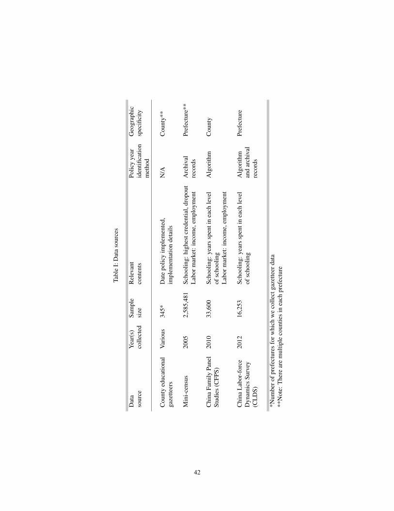
Tabl

eI:

Dat

aso

urce

s

Dat

aYe

ar(s

)Sa

mpl

eR

elev

ant

Polic

yye

arG

eogr

aphi

cso

urce

colle

cted

size

cont

ents

iden

tifica

tion

spec

ifici

tym

etho

d

Cou

nty

educ

atio

nal

Vario

us34

5*D

ate

polic

yim

plem

ente

d,N

/AC

ount

y**

gaze

tteer

sim

plem

enta

tion

deta

ils

Min

i-cen

sus

2005

2,58

5,48

1Sc

hool

ing:

high

estc

rede

ntia

l,dr

opou

tA

rchi

val

Pref

ectu

re**

Labo

rmar

ket:

inco

me,

empl

oym

ent

reco

rds

Chi

naFa

mily

Pane

l20

1033

,600

Scho

olin

g:ye

ars

spen

tin

each

leve

lA

lgor

ithm

Cou

nty

Stud

ies

(CFP

S)of

scho

olin

gLa

borm

arke

t:in

com

e,em

ploy

men

t

Chi

naLa

bor-

forc

e20

1216

,253

Scho

olin

g:ye

ars

spen

tin

each

leve

lA

lgor

ithm

Pref

ectu

reD

ynam

ics

Surv

eyof

scho

olin

gan

dar

chiv

al(C

LDS)

reco

rds

*Num

bero

fpre

fect

ures

forw

hich

we

colle

ctga

zette

erda

ta**

Not

e:Th

ere

are

mul

tiple

coun

ties

inea

chpr

efec

ture

42

Table II: Effects of the policy on schooling outcomes - average treatment effects

Outcome CFPS 2005 CensusProbability: at least six .547***years of primary school (.0294)

Years spent in all levels .66***of school (.209)

Years of post-primary .0928schooling (.204)

Highest credential: at least .00368 -.00495middle school (.0319) (.00303)

Highest credential: at least .000299 .00628*high school (.0263) (.00327)

Dropped out of school, -.00017any level (.00137)

Observations in sample 2,680 243,548

* p<0.10, ** p<0.05, *** p<0.01. Each cell presents a treatment effect estimate from a separateregression with the relevant robust standard error below, in parentheses. Standard errors areclustered at the county (CFPS) or prefecture (census) level.

43

Table III: Effects of the policy on schooling outcomes for vulnerable subgroups

Outcome Female Rural Rural femaleYears of post-primary schoolingCFPS -0.2020 0.2357 -0.0472

(0.2951) (0.2673) (0.4008)Graduated from middle schoolCFPS -0.0355 0.0550 0.0304

(0.0498) (0.0462) (0.0696)

Census -0.0057 -0.0049 -0.0044(0.0043) (0.0046) (0.0063)

Graduated from high schoolCFPS -0.0221 0.0238 0.0133

(0.0400) (0.0195) (0.0352)

Census 0.0043 -0.0016 -0.0030(0.0039) (0.0025) (0.0028)

Dropped out of school, any levelCensus 0.0037* -0.0003 0.0047*

(0.0019) (0.0021) (0.0028)

Observations in CFPS sample 1,277 1,293 592Observations in Census sample 126,081 157,308 81,490

* p<0.10, ** p<0.05, *** p<0.01. Each cell presents a treatment effect estimate from a separateregression with the relevant robust standard error below, in parentheses. Standard errors areclustered at the county (CFPS) or prefecture (census) level.

44

Table IV: Effects of the policy on labor market outcomes

Outcome EstimatesPanel A: average treatment effectsCurrently employed 0.0026

(0.0052)

Works for government 0.0035(0.0062)

Log of monthly income, using cohort and place 0.0194***fixed effects (0.0073)

Log of monthly income using cohort, place, and 0.0203***cohort-by-region fixed effects (0.0071)

Panel B: effect on log of monthly income, by highest credential†

Primary school 0.0694***(0.0279)

Middle school 0.0503***(0.0095)

High school 0.0257***(0.0092)

Tertiary schooling -0.0098(0.0093)

Panel C: effect on log of monthly income, by genderMen 0.0081

(0.0085)

Women 0.0375***(0.0086)

Panel D: effect on log of monthly income, by employerGovernment -0.0139

(0.0086)

Enterprise 0.0327***(0.0076)

* p<0.01, ** p<0.05, *** p<0.01. Data: census. For first row, N=86,240. For all other regressions,N=66,425. Panel A presents results from four different regressions. In panels B, C, and D, wepresent coefficients from a single regression as specified in the panel title. Panels B, C, and Dpresent coefficients of a dummy variable for membership in the group given in the left column(e.g. those whose highest credential is primary school) interacted with the treatment dummy. Allsamples include only urban residents and non-migrants. Robust standard errors are given belowthe coefficient estimate in parentheses and are clustered at prefecture level. †Panel B coefficients,when weighted by proportion of sample given in column 4 of Table V, sum to 0.0213.

45

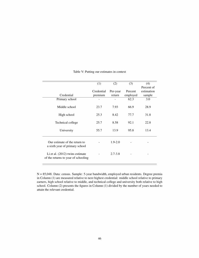
Table V: Putting our estimates in context

(1) (2) (3) (4)Percent of

Credential Per-year Percent estimationCredential premium return employed sample

Primary school - - 62.3 3.0

Middle school 23.7 7.93 66.9 28.9

High school 25.3 8.42 77.7 31.8

Technical college 25.7 8.58 92.1 22.8

University 55.7 13.9 95.8 13.4

Our estimate of the return to - 1.9-2.0 - -a sixth year of primary school

Li et al. (2012) twins estimate - 2.7-3.8 - -of the returns to year of schooling

N = 85,048. Data: census. Sample: 5-year bandwidth, employed urban residents. Degree premiain Column (1) are measured relative to next highest credential: middle school relative to primaryearners, high school relative to middle, and technical college and university both relative to highschool. Column (2) presents the figures in Column (1) divided by the number of years needed toattain the relevant credential.

46

Table VI: Cost-benefit calculation: 1981-2050

Assumption about heterogeneityin b1 by highest credential held

b1 estimate Using average Using credential-specificused for rural areas treatment effect for all treatment effects

Using estimates from urban areas -36,462 34,902

Using rural effect estimates from our data -82,390 -212,220

Costs 178,497 -

Cost-benefit calculation for cohort leaving -456.4primary school in 2014 (urban b1, average b1 )

*Estimates in millions of 2015 US Dollars. See Section VI for details on calculations.

47

FIGURES

Figure I: Length of each credential, pre- and post-policy

Primary

Middle

High

Tertiary

Primary

Middle

High

Tertiary

1

2

3

4

5

6

7

9

10

11

12

13

14

15

16

Years of schooling

Pre-policy Post-policy

Extra year

Pre-policymedian and mode = 8 Same years of schooling

Same credential

New decision

This figure depicts the length and structure of the Chinese education system before the policy isimplemented in the left column, and after the policy is implemented in the right column. The y-axis represents the number of years needed to complete a credential under normal circumstances.Before the policy, it took five years to finish a primary school credential, as represented by theheight of the box labeled “Primary” in the left column. Middle, High, and Tertiary refer to juniorhigh school, senior high school, and university, respectively. To finish Middle School before thepolicy is implemented, an individual would need 8 years of school - five years of Primary andthree of Middle, which can be read from the top line of the “Middle” box. The dashed bold linestemming from the y-axis at y = 8 indicates that prior to the policy, the median and mode of yearsof schooling is 8. The right column depicts the change introduced by the policy, adding an extrayear to the time it takes to attain a Primary credential. The lines connecting the left and rightcolumn depict the change in the total number of years it takes to earn each credential. The dashedred lines show the trade-off that the modal student faces after the policy.

48

Figure II: Predetermined characteristics across the treatment threshold

.02

.04

.06

Relative cohort size

.45

.5

.55

Proportion female

.25

.35

.45

−10 0 10Distance to treatment year

Proportion with urban household registry

49

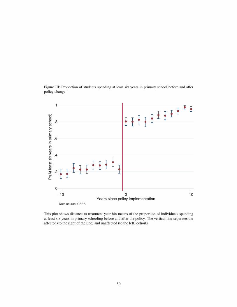
Figure III: Proportion of students spending at least six years in primary school before and afterpolicy change

0

.2

.4

.6

.8

1

Pr(

At

lea

st s

ix y

ea

rs in

prim

ary

sch

oo

l)

−10 0 10Years since policy implementation

Data source: CFPS

This plot shows distance-to-treatment-year bin means of the proportion of individuals spendingat least six years in primary schooling before and after the policy. The vertical line separates theaffected (to the right of the line) and unaffected (to the left) cohorts.

50

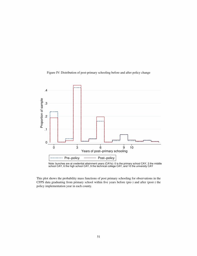
Figure IV: Distribution of post-primary schooling before and after policy change

0

.1

.2

.3

.4

Pro

po

rtio

n o

f sa

mp

le

0 3 6 9 10Years of post−primary schooling

Pre−policy Post−policy

Note: bunches are at credential attainment years (CAYs): 0 is the primary school CAY, 3 the middleschool CAY, 6 the high school CAY, 9 the technical college CAY, and 10 the university CAY

This plot shows the probability mass functions of post primary schooling for observations in theCFPS data graduating from primary school within five years before (pre-) and after (post-) thepolicy implementation year in each county.

51

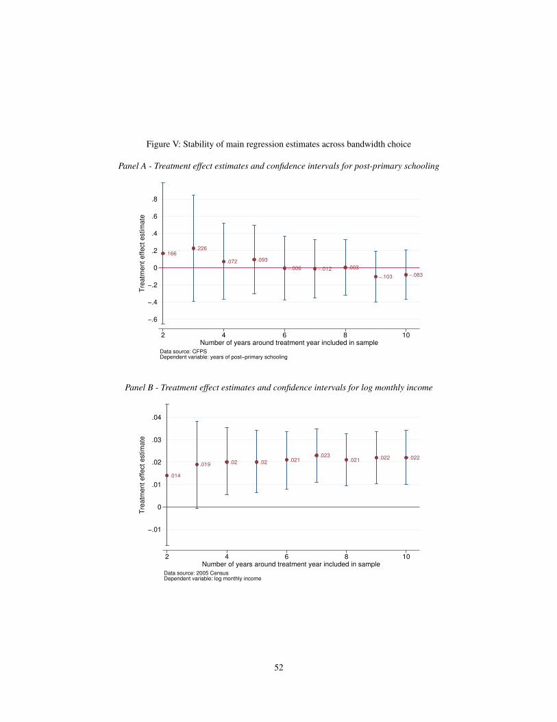
Figure V: Stability of main regression estimates across bandwidth choice

Panel A - Treatment effect estimates and confidence intervals for post-primary schooling

.166.226

.072 .093

−.006 −.012 .003

−.103 −.083

−.6

−.4

−.2

0

.2

.4

.6

.8

Tre

atm

ent effect

est

imate

2 4 6 8 10Number of years around treatment year included in sample

Data source: CFPSDependent variable: years of post−primary schooling

Panel B - Treatment effect estimates and confidence intervals for log monthly income

.014

.019 .02 .02 .021.023

.021 .022 .022

−.01

0

.01

.02

.03

.04

Tre

atm

ent effect

est

imate

2 4 6 8 10Number of years around treatment year included in sample

Data source: 2005 CensusDependent variable: log monthly income

52

Figure VI: Monte Carlo analysis - distribution of effect estimates of placebo treatment on logmonthly income from 1,000 draws of placebo years

Density

−.04 −.02 0 .02 .04Treatment effect estimate

Data source: 2005 census

Our estimate

Mean + / - twostandard deviations

53

Figure VII: Kernel density of cognitive skills test score, by treatment status

Density

0 .2 .4 .6 .8 1Ability test score

Untreated Treated

Data source: CFPS

This plot shows the kernel density of cognitive skills test scores for observations from the CFPSdata, plotted separately for those in affected and unaffected cohorts, in the five year bandwidthsample.

54

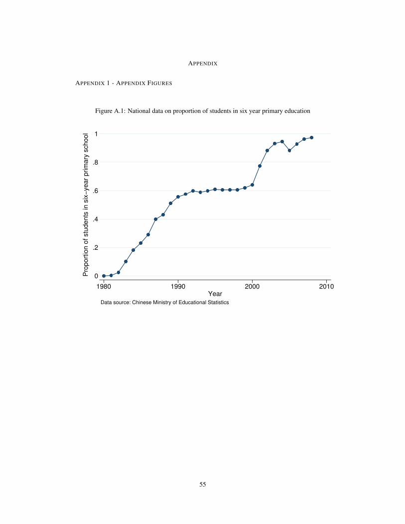
APPENDIX

APPENDIX 1 - APPENDIX FIGURES

Figure A.1: National data on proportion of students in six year primary education

0

.2

.4

.6

.8

1

Pro

po

rtio

n o

f st

ud

en

ts in

six

−ye

ar

prim

ary

sch

oo

l

1980 1990 2000 2010Year

Data source: Chinese Ministry of Educational Statistics

55

Figure A.2: Timing of implementation by prefecture

Note: In some cases, prefecture boundaries have changed since the archive was published. Inthese cases, we take the prefecture level-average of the treatment year in all previous prefecturecapitals falling within the new prefecture. In prefectures that are colored white, we are unable toassign a unique prefecture-level treatment year for reasons discussed in Section III.

56

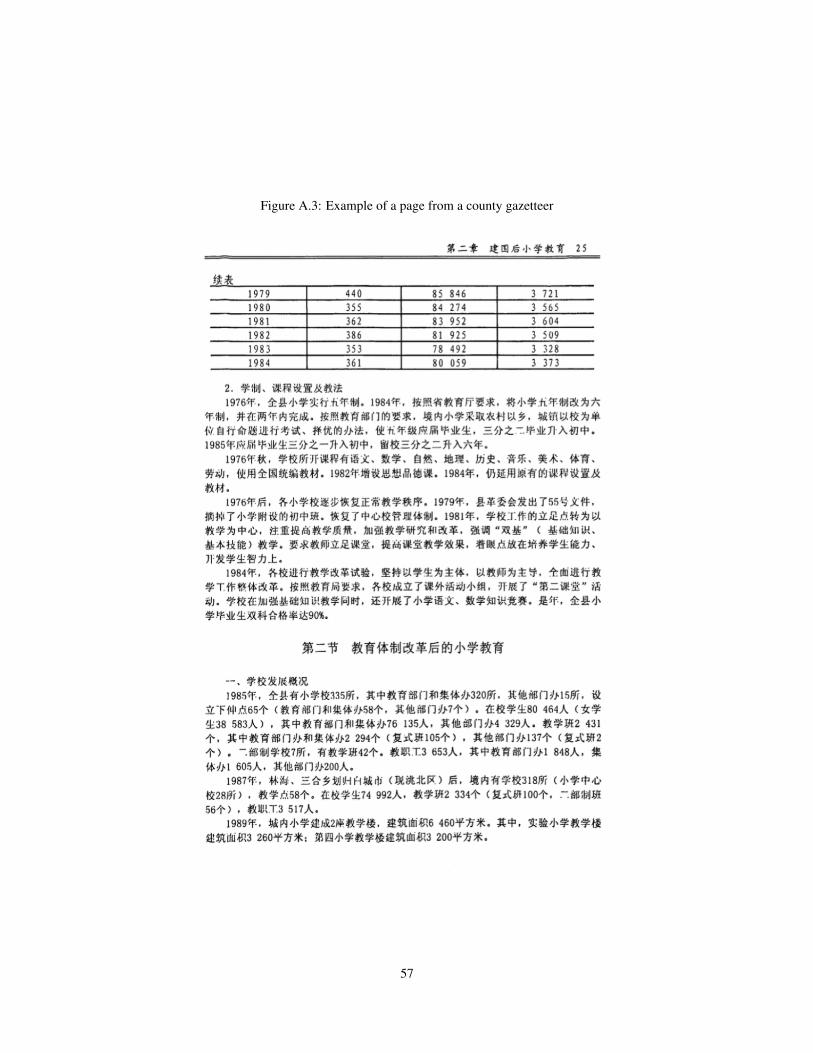
Figure A.3: Example of a page from a county gazetteer

57

Figure A.4: Example of mean shift algorithm identifying year of policy implementation

16

18

20

22

24

26

Su

m o

f sq

ua

red

re

sid

ua

ls

4

5

6

7

Me

an

ye

ars

of

prim

ary

sch

oo

l

1975 1980 1985 1990 1995 2000 2005 2010Year graduated from primary school

Mean years of primary school

Sum of squared residuals, mean shift regression

Data source: CFPS

58

Figure A.5: Mean schooling levels before and after policy implementation, by distance to treat-ment year cohort

7

8

9

10

11

Total years

of schooling

Raw data

−1

0

1

Cohort fixed effects removed

2

3

4

5

Years of

post−primary

schooling

−10 0 10Distance to treatment year

−1

0

1

−10 0 10Distance to treatment year

Data source: CFPS

59

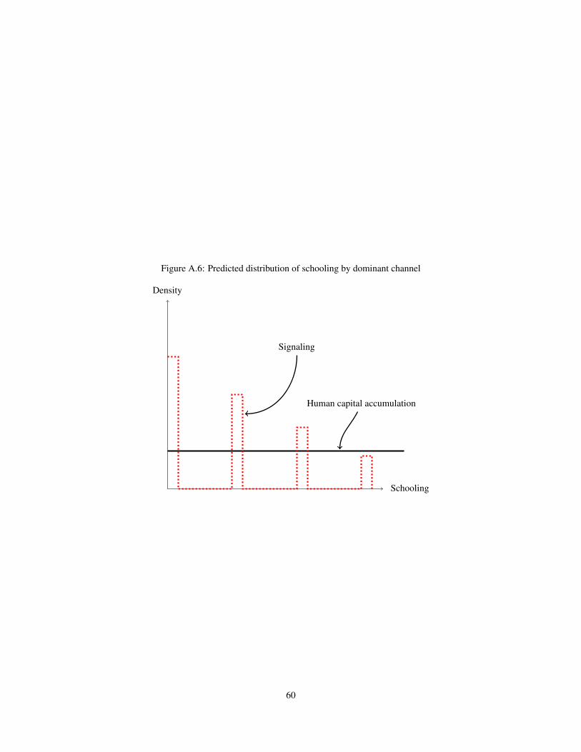
Figure A.6: Predicted distribution of schooling by dominant channel

Schooling

Density

Signaling

Human capital accumulation

60

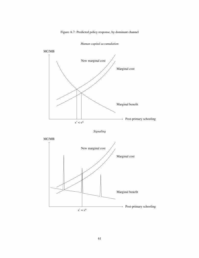
Figure A.7: Predicted policy response, by dominant channel

Human capital accumulation

Post-primary schooling

MC/MB

Marginal benefit

Marginal cost

New marginal cost

s’ < s*

Signaling

Post-primary schooling

MC/MB

Marginal benefit

Marginal cost

s’ = s*

New marginal cost

61

Figure A.8: Incorporating heterogeneity in wealth and genetic endowment into our model

Panel A: The schooling ascent threshold in the wealth/endowment space

Geneticendowment

Wealth

Wealth threshold

Endowment threshold

e

w

School ascent threshold

sa = 0

sa = 1

Panel B: The predicted impact of the policy on schooling ascent

Geneticendowment

Wealth

New wealth thresholdw0

Effect one:school more costly

e

w

sa = 0

sa = 1

New endowment threshold

e0

Effect two: entranceexam easier

62

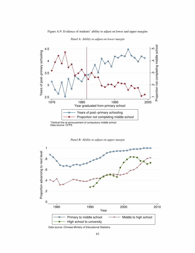
Figure A.9: Evidence of students’ ability to adjust on lower and upper margins

Panel A: Ability to adjust on lower margin

.1.2

.3.4

.5P

rop

ort

ion

no

t co

mp

letin

g m

idd

le s

cho

ol

2.5

3

3.5

4

4.5

Ye

ars

of

po

st−

prim

ary

sch

oo

ling

1976 1985 1995 2005Year graduated from primary school

Years of post−primary schooling

Proportion not completing middle school

*Vertical line at annoucement of compulsory middle schoolData source: CFPS

Panel B: Ability to adjust on upper margin

0

.2

.4

.6

.8

1

Pro

po

rtio

n a

dva

nci

ng

to

ne

xt le

vel

1980 1990 2000 2010Year

Primary to middle school Middle to high school

High school to university

Data source: Chinese Ministry of Educational Statistics

63

Figure A.10: National statistics and province-level CDFs of policy implementation

First 12 provinces

0.2.4.6.81

1980 1990 2000 2010Year

Anhui

0.2.4.6.81

1980 1990 2000 2010Year

Beijing

0.2.4.6.81

1980 1990 2000 2010Year

Chongqing

0.2.4.6.81

1980 1990 2000 2010Year

Fujian

0.2.4.6.81

1980 1990 2000 2010Year

Gansu

0.2.4.6.81

1980 1990 2000 2010Year

Guangdong

0.2.4.6.81

1980 1990 2000 2010Year

Guangxi

0.2.4.6.81

1980 1990 2000 2010Year

Guizhou

0.2.4.6.81

1980 1990 2000 2010Year

Hebei

0.2.4.6.81

1980 1990 2000 2010Year

Heilongjiang

0.2.4.6.81

1980 1990 2000 2010Year

Henan

0.2.4.6.81

1980 1990 2000 2010Year

Hubei

These plots show the proportion of individuals enrolled in six-year primary schools in the 24 non-Shanghai CFPS provinces. The sequence of hollow circles represent the proportion of treatedcounties in a given province by year according to county-specific implementation years identifiedin the CFPS data. The sequence of solid circles are from publicly available, Chinese Ministryof Education statistics on the number of schoolchildren benefiting from six year education in agiven province by year. Measurement error and policy experimentation cause these to brieflytrend downward in a few cases.

64

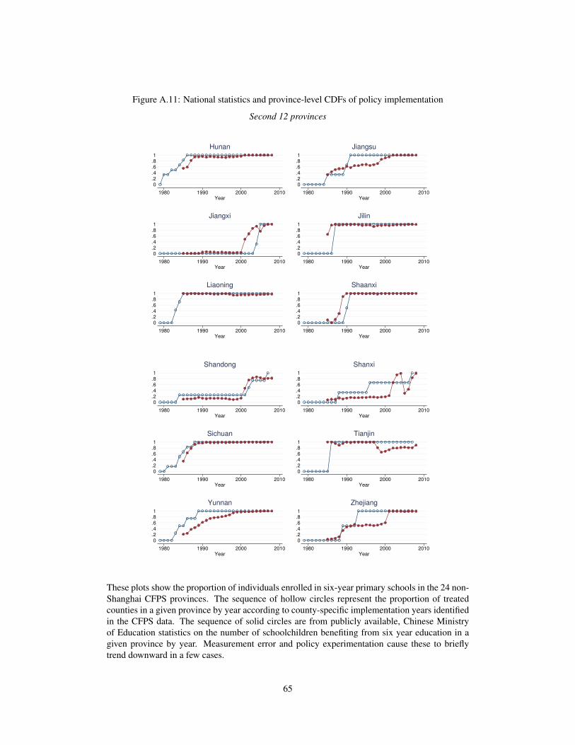
Figure A.11: National statistics and province-level CDFs of policy implementation

Second 12 provinces

0.2.4.6.81

1980 1990 2000 2010Year

Hunan

0.2.4.6.81

1980 1990 2000 2010Year

Jiangsu

0.2.4.6.81

1980 1990 2000 2010Year

Jiangxi

0.2.4.6.81

1980 1990 2000 2010Year

Jilin

0.2.4.6.81

1980 1990 2000 2010Year

Liaoning

0.2.4.6.81

1980 1990 2000 2010Year

Shaanxi

0.2.4.6.81

1980 1990 2000 2010Year

Shandong

0.2.4.6.81

1980 1990 2000 2010Year

Shanxi

0.2.4.6.81

1980 1990 2000 2010Year

Sichuan

0.2.4.6.81

1980 1990 2000 2010Year

Tianjin

0.2.4.6.81

1980 1990 2000 2010Year

Yunnan

0.2.4.6.81

1980 1990 2000 2010Year

Zhejiang

These plots show the proportion of individuals enrolled in six-year primary schools in the 24 non-Shanghai CFPS provinces. The sequence of hollow circles represent the proportion of treatedcounties in a given province by year according to county-specific implementation years identifiedin the CFPS data. The sequence of solid circles are from publicly available, Chinese Ministryof Education statistics on the number of schoolchildren benefiting from six year education in agiven province by year. Measurement error and policy experimentation cause these to brieflytrend downward in a few cases.

65

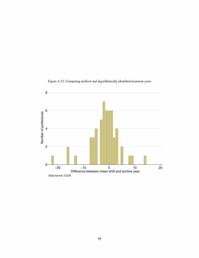
Figure A.12: Comparing archival and algorithmically identified treatment years

0

2

4

6

8

Nu

mb

er

of

pre

fect

ure

s

−20 −10 0 10 20Difference between mean shift and archive year

Data source: CLDS

66

APPENDIX 2 - APPENDIX TABLES

Table A.1: Anecdotes on implementation of six year primary education from across China

Locality Strategy of Changing 5-Year to 6-Year Primary Education SourceBeijing In 1969, the length of primary education was shortened to five

years. Starting from September 1st, 1980, the length of primaryeducation was prolonged to six years, with the fifth-grade

students continuing to be in the old system and students of othergrades entering into the new system.

BeijingGeneral

EducationChronicle

(Part I)Xinle

County,Hebei

Province

In 1967, the length of primary education was shortened to fiveyears. Starting from August 1985, first-grade students and one

half of second-grade students entered into the new six yearsystem, while the rest of students remained in the old system.

XinleEducationalChronicle

NanjingCity,

JiangsuProvince

In 1969, the length of primary education was shortened to fiveyears. Starting from 1982, the length of primary education was

prolonged to six years in urban districts and children startedprimary education at the age of six. By contrast, the length ofprimary education remained to be five years until 1999 in five

other counties (Jiangning, Jiangpu, Liuhe, Gaochun, andLishui).

NanjingEducationalChronicle

WuyiCounty,ZhejiangProvince

In 1984, first-grade students entered into the new six yearsystem in half of primary schools, with the other half following

the next year. In 1987, however, all primary schools wererequired to resume the five year system. In September 1999, allprimary schools were restored to the new system of six years.The final cohort under the old system graduated in June 2004.

WuyiEducationalChronicle

DongyingDistrict,

ShandongProvince

In 1997, the compulsory education system changed from the5-3 (years of primary school-years of middle school) to the 5-4system. In 2003, first-grade students entered into the new 6-3

system.

DongyingDistrict

Chronicle(1998-2005)

XishuiCounty,Hubei

Province

In 1986, the first-grade students entered into the new 6-3 systemin the primary schools located in county seats, while other

primary schools remained in the old 5-3 system. In 1987, thefirst-grade students in the primary schools located in the

township entered into the new 6-3 system. In 1991, first-gradestudents in the remaining primary schools entered into the new

6-3 system.

XishuiEducationalChronicle

(1986-2006)

67

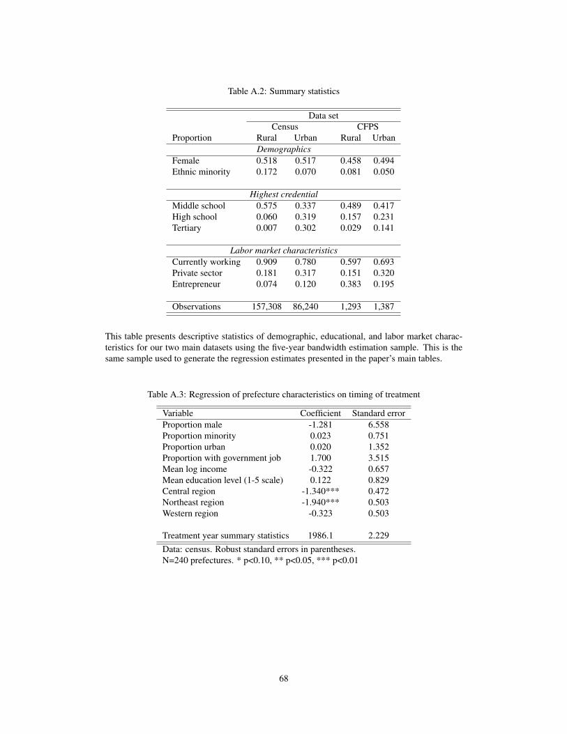
Table A.2: Summary statistics

Data setCensus CFPS

Proportion Rural Urban Rural UrbanDemographics

Female 0.518 0.517 0.458 0.494Ethnic minority 0.172 0.070 0.081 0.050

Highest credentialMiddle school 0.575 0.337 0.489 0.417High school 0.060 0.319 0.157 0.231Tertiary 0.007 0.302 0.029 0.141

Labor market characteristicsCurrently working 0.909 0.780 0.597 0.693Private sector 0.181 0.317 0.151 0.320Entrepreneur 0.074 0.120 0.383 0.195

Observations 157,308 86,240 1,293 1,387

This table presents descriptive statistics of demographic, educational, and labor market charac-teristics for our two main datasets using the five-year bandwidth estimation sample. This is thesame sample used to generate the regression estimates presented in the paper’s main tables.

Table A.3: Regression of prefecture characteristics on timing of treatment

Variable Coefficient Standard errorProportion male -1.281 6.558Proportion minority 0.023 0.751Proportion urban 0.020 1.352Proportion with government job 1.700 3.515Mean log income -0.322 0.657Mean education level (1-5 scale) 0.122 0.829Central region -1.340*** 0.472Northeast region -1.940*** 0.503Western region -0.323 0.503

Treatment year summary statistics 1986.1 2.229Data: census. Robust standard errors in parentheses.N=240 prefectures. * p<0.10, ** p<0.05, *** p<0.01

68

APPENDIX 3 - DETAILS ON OUR USE OF THE MEAN SHIFT MODEL

As we use an algorithm to determine treatment year status for observations in the CFPS, we

introduce a few safeguards to ensure that we are not erroneously choosing a year when there is no

change in treatment status or not enough evidence to determine the year. Specifically, we exclude

counties in which:

1. The cohort-level median number of years of primary school in a given county is never less

than 5.5 before the identified treatment year or is never more than 5.5 after;

2. The mean shift model predicts a treatment year after which individuals have less primary

schooling, that is, g1 < 0 in equation 1;

3. There are more than four cohorts for which we have no observations within five years

before or after the identified treatment year (that is, data for at least five of the ten cohorts

in this county’s restricted bandwidth sample are missing).

This exercise excludes 32 of the 144 non-Shanghai counties, or about 78% of the sample. All of

the results we show are qualitatively similar with the entire 144 county sample and are available

by request.

As a final check of accuracy, we visually compare the treatment year generated by the mean

shift model to each county’s histogram. In four cases, our inspection of the histograms suggested

a year more than one year different than the mean shift model’s choice and we use this visu-

ally identified year in our main analyses, controlling for those counties whose year was chosen

visually as opposed to algorithmically.

To check that these algorithmically identified years are credible, we conduct two exercises.

First, we compare the mean shift years for all counties within each province to national statistics

on provincial-level implementation, shown in Appendix Figures A.10 and A.11. The two series

track closely and their correlation is 0.7759. Second, we apply both the mean shift and archival

match policy year identification methods to the China Labor-force Dynamics Survey data. Ap-

pendix Figure A.12 shows the distribution of the difference between archival and algorithmically

identified treatment years. These values are normally distributed around 0, and in 67% of prefec-

tures the years identified by the two methods are within 3 years of each other. This amount of

69

discrepancy is not surprising, as in the gazetteers we see that counties occasionally implemented

at different times within a prefecture. Additionally, the number of observations in cohort-by-

prefecture bins in the Labor-force Dynamics dataset is small, which implies imprecision (relative

to using the CFPS) in our ability to algorithmically determine the implementation year.

APPENDIX 4 - DETAILS OF COST-BENEFIT ANALYSIS

This section outlines our data sources and extrapolation assumptions for the cost benefit analysis

we perform. The costs of the policy we include consist of one year of forgone wages for all

affected individuals. We assume the value of one individual’s forgone year of wages is equal

to a⇤GDPtNt

, where Nt is the size of the active workforce in year t. We calculate if and when the

forgone year falls for each individual born on or after 1969 (as the first affected cohort would

be leaving primary school in 1981). To calculate the total number losing a given year in each

cohort, we multiply the total number of individuals in each cohort (generated using data from

the Chinese National Statistical Bureau and World Bank World Development Indicators data) by

the proportion of individuals with a given credential in each cohort (calculated from the CLDS

data). We assume the lost year is the year a person would have entered the labor force in the

absence of the policy, e.g. for someone who was born in 1980 and finishes school with a middle

school credential, we calculate the value of the work they would have done in 1995 when they

would have left school in the absence of the policy (starting school at age 7, spending five years

in primary school and three years in middle school). We assume that those leaving school after

primary school do not lose a year of work, as they will leave school at the age of 12 and are not

likely to immediately enter gainful employment. For simplicity, we assume that everyone enters

school at age 7.

The benefits from the policy consist of the boost in earnings we estimate for affected individu-

als accruing throughout their lives. This parameter is taken directly from our estimates in Section

V. We assume that the benefits affected individuals enjoy are constant throughout their lifetimes,

and calculate the total value of the earnings gain for each affected individual up to the year 2050.

Table A.4 provides our data sources for each of these figures and assumptions used to extrapolate

into the future and where data is not available.

We exclude a few potential sources of costs and benefits, believing them to be several orders

of magnitude smaller than the lost year of wages and the lifetime of income gains. On the costs

70

side, we exclude the cost of hiring new teachers and the cost of building new facilities. We do so

because archival records suggest that in the short term, the current staff was used to meet most of

the increased personnel needs imposed by the policy and classrooms could be split, thus requiring

no sizable infrastructure additions. In the long term, the one child policy reduced the number of

children in schools, and so existing staff levels and infrastructure house a smaller and smaller

number of children. We assume that this would largely offset the need for long term staff and

infrastructure adjustments to accommodate the extra cohort of primary students. On the benefits

side, we disregard the possible benefit of the creation of new teacher jobs, as our assumption

about the staffing costs of the policy implies very few additional jobs would be created. As in

Duflo’s approach, we exclude the possible beneficial impact of the extra year of schooling on

health, fertility and other non-financial outcomes.

71

Tabl

eA

.4:C

ost-b

enefi

tcal

cula

tion

deta

ils

Ran

geR

ange

for

Dat

apo

int

Sour

ceof

data

extra

pola

tion

Ass

umpt

ions

used

Wha

tuse

dfo

rN

otes

Birt

hra

tepe

rst

ats.

gov.

cn19

66-2

013

N/A

N/A

Size

ofco

hort

Ass

ume:

coho

rtsi

ze1,

000

wom

enco

nsta

nt20

13-2

050

Num

bero

fwom

enst

ats.

gov.

cn19

70-2

013

N/A

N/A

Size

ofco

hort

-

Tota

llab

orfo

rce

Wor

ldB

ank

WD

I19

81-2

015,

Gap

sin

Line

artre

ndTo

tall

abor

forc

eC

lose

to(W

orld

Dev

.fiv

e-ye

arly

estim

ates

for

betw

een

stat

s.go

v.cn

figur

es,

Indi

cato

rs)

estim

ates

2020

-205

0es

timat

esbu

twith

pred

ictio

nsfo

r202

0-20

50to

2050

Prop

ortio

nof

coho

rtC

hina

Labo

r-fo

rce

Birt

hco

horts

Birt

hco

horts

Line

artre

nds

from

CB

estim

ates

with

Beg

inex

trapo

latio

nat

with

each

Dyn

amic

sSu

rvey

1969

-198

719

87-2

035

prev

ious

9ye

ars

and

coho

rt-sp

ecifi

cef

fect

s19

87co

hort

toav

oid

educ

atio

nle

vel

(CLD

S)ru

les

ofpr

obab

ility

mea

sure

men

terr

or(0

P

1)

Prop

ortio

nof

coho

rtC

hina

’sN

atio

nal

1981

-201

020

10-2

050

Full

cove

rage

Prop

ortio

naf

fect

edEq

uate

5ye

araf

fect

edby

polic

yB

urea

uof

afte

r201

0by

polic

ypr

imar

y+

4ye

arSt

atis

tics

mid

dle

with

6pr

imar

y+

3m

iddl

e

Alp

ha(la

bor’s

shar

eK

arab

arbo

unis

and

1992

-200

919

81-1

991

1981

-91:

aver

age

ofA

rgum

enti

nfin

al-

ofG

DP)

Nei

man

(201

4)20

10-2

050

t+1

tot+

3;ca

lcul

atio

n20

10-5

0:av

erag

eof

t-1to

t-3

GD

P(c

onst

ant

Wor

ldB

ank

WD

I19

81-2

013

2014

-205

0G

row

thra

tede

clin

esA

rgum

enti

nfin

al-

2005

US$

)an

nual

lyfr

om20

13ca

lcul

atio

nra

teto

4%,a

nnua

lde

crea

seof

0.15

%

72