the importance of multimodel projections to assess...

Ecological Applications, 19(7), 2009, pp. 1680–1692� 2009 by the Ecological Society of America

The importance of multimodel projections to assess uncertaintyin projections from simulation models

DENIS VALLE,1,2,4 CHRISTINA L. STAUDHAMMER,1 WENDELL P. CROPPER, JR.,1 AND PAUL R. VAN GARDINGEN3

1School of Forest Resources and Conservation, University of Florida, Gainesville, Florida 32611 USA2Projeto Dendrogene, Empresa Brasileira de Pesquisa Agropecuaria (EMBRAPA), Caixa Postal 48, Belem, Para 66095-100, Brazil

3School of GeoSciences, The University of Edinburgh, Edinburgh EH8 9XP United Kingdom

Abstract. Simulation models are increasingly used to gain insights regarding the long-term effect of both direct and indirect anthropogenic impacts on natural resources and todevise and evaluate policies that aim to minimize these effects. If the uncertainty fromsimulation model projections is not adequately quantified and reported, modeling resultsmight be misleading, with potentially serious implications. A method is described, based on anested simulation design associated with multimodel projections, that allows the partitioningof the overall uncertainty in model projections into a number of different sources ofuncertainty: model stochasticity, starting conditions, parameter uncertainty, and uncertaintythat originates from the use of key model assumptions. These sources of uncertainty are likelyto be present in most simulation models. Using the forest dynamics model SYMFOR as a casestudy, it is shown that the uncertainty originated from the use of alternate modelingassumptions, a source of uncertainty seldom reported, can be the greatest source ofuncertainty, accounting for 66–97% of the overall variance of the mean after 100 years ofstand dynamics simulation. This implicitly reveals the great importance of these multimodelprojections even when multiple models from independent research groups are not available.Finally, it is suggested that a weighted multimodel average (in which the weights are estimatedfrom the data) might be substantially more precise than a simple multimodel average(equivalent to equal weights for all models) as models that strongly conflict with the data aregiven greatly reduced or even zero weights. The method of partitioning modeling uncertaintyis likely to be useful for other simulation models, allowing for a better estimate of theuncertainty of model projections and allowing researchers to identify which data need to becollected to reduce this uncertainty.

Key words: model uncertainty; modeling assumptions; multimodel; partitioning of the variance;simulation model.

INTRODUCTION

Sustainable use of natural resources and the balance

between satisfying human needs and maintaining other

ecosystem functions will require quantitative knowledge

about the ecosystem’s present and future responses (Clark

et al. 2001, DeFries et al. 2004). Numerous models have

been created to predict ecosystem responses to direct and

indirect anthropogenic influence, but if the uncertainty

associated with these model projections is not reported

adequately, confidence of projections cannot be assessed.

At one extreme, thismay result in overconfident decisions,

while at the other, decisionmakers may use it as an excuse

to postpone or avoid making necessary decisions.

The field of statistics has traditionally acknowledged

parametric uncertainty once a particular model form has

been chosen. The exclusion of model structure and

model selection uncertainty has been shown, however, to

result in overly optimistic predictive or inferential un-

certainty, which can have serious implications (Draper

1995, Hoeting et al. 1999). The problem of ignoring

model structure uncertainty is likely to be exacerbated in

situations in which model extrapolations from available

data are needed for decision making, as models that are

very different mathematically can have similar fits to the

data but wildly different predictions outside the data

range (Chatfield 1995, Draper 1995). Multimodel in-

ference has been suggested as a robust method that cir-

cumvents the problem of overly optimistic predictive or

inferential uncertainty through improved representation

of model structure uncertainty (Burnham and Anderson

1998, Wintle et al. 2003, Ellison 2004, Link and Barker

2006).

As in the field of statistics, probably the most-studied

source of uncertainty in simulation modeling in the

ecological literature is parameter estimate uncertainty.

Parameter uncertainty has been assessed in population

viability analysis (e.g., Ellner and Fieberg 2003), as well

as in models of forest (e.g., Pacala et al. 1996), climate

Manuscript received 22 August 2008; revised 15 January2009; accepted 20 January 2009. Corresponding Editor: Y. Luo.

4 Present address: University Program in Ecology, DukeUniversity, Durham, North Carolina 27708 USA.E-mail: [email protected]

1680

(e.g., Wigley and Raper 2001, Murphy et al. 2004,

Stainforth et al. 2005), and disease (e.g., Elderd et al.2006). Other sources of uncertainty that are commonly

reported in simulation models include model stochas-ticity (e.g., Gourlet-Fleury et al. 2005, Degen et al. 2006)

and effect of starting conditions (e.g., simulationsinitialized with different forest plots; Phillips et al.2004, van Gardingen et al. 2006). Model stochasticity is

defined here as the changes in model projections,simulated with a fixed model structure and fixed

parameter values, solely due to the stochastic nature ofthe simulated processes (e.g., mortality and recruit-

ment). Model structure uncertainty, on the other hand,is defined here as the changes in model projections due

to changes in the structure of the model (e.g., changes inthe form of the underlying equations). Because of the

large number of general circulation and terrestrialbiogeochemistry models built by independent research

groups, multimodel projections have been increasinglyused for regional and global climate and vegetation

predictions. This has allowed for the assessment of therobustness of these predictions in relation to the choice

of the model (Cramer et al. 1999, Cox et al. 2008, Malhiet al. 2008). The evaluation of model structure un-certainty for other types of simulation models such as

those used for management of natural resources,however, is still uncommon (but see Pascual et al.

1997, Carpenter 2002, Bradshaw et al. 2006).The objective of this study is to show that, even if

multiple models built by independent research groupsare not available, multimodel inference is still a valuable

tool to assess the uncertainty that originates from theuse of key assumptions adopted in the process of model

building. In particular, multimodel projections are usedto show how the uncertainty resulting from these

assumptions can be larger than the uncertainty thatarises from other more commonly assessed sources, such

as parameter uncertainty, model stochasticity, and effectof starting conditions. To achieve this objective, the

method used to partition the overall uncertainty intothese different sources is described and a comparison of

the uncertainty originating from these sources is madeusing the forest dynamics model SYMFOR as a casestudy. Finally, the broader implications of the results

from this case study are discussed and general recom-mendations for ecological modelers are provided.

METHODS

The data set

The series of plots at the Tapajos National Forest,Para, Brazil, are clustered in two regions known as km

67 and km 114. The series of plots at km 114 arecomposed of 60 permanent sample plots (PSPs), each of

0.25 ha, initially measured (all trees with diameter atbreast height [dbh] �5 cm) in 1981 in an unloggedprimary forest. Twelve of these plots were left unlogged

while a silvicultural experiment with a randomized blockdesign was installed in the remaining 48 plots. In this

silvicultural experiment, all plots were selectively logged

in 1982 and different thinning intensity treatments were

applied in 1995. The series of plots at km 67 are

composed of 36 PSPs, each of 0.25 ha. This region wasselectively logged in 1979, two years prior to the in-

stallation of the permanent plots (in 1981). Detailed

description of the forest and these experiments can be

found elsewhere (Silva et al. 1995, 1996, Alder and Silva2000, Phillips et al. 2004, Oliveira 2005). This data set

was used to calibrate and to initialize SYMFOR

(Phillips et al. 2004).

The model and its variants

SYMFOR is a modeling framework for mixed

tropical forest that combines a management model with

an empirical spatially explicit individual-tree-based

ecological model. The management model allows users

to specify silvicultural activities, such as harvest, thin-ning, poisoning, and enrichment planting; the ecological

model simulates the natural processes of recruitment,

growth, and mortality. SYMFOR has been extensively

used for tropical forest management issues in Indonesia(Phillips et al. 2002, 2003, van Gardingen et al. 2003),

Brazil (Phillips et al. 2004, van Gardingen et al. 2006,

Valle et al. 2007), and Guyana (vanUlft 2004, Arets

2005).

A brief summary of the model, which is described in

greater detail elsewhere (Phillips et al. 2004), follows.First, because of the high diversity of tree species present

in the data set (see Plate 1), species were assigned to one

of 10 ecological species groups using a three-stage

method. Cluster analysis, discriminant analysis, and

subjective assignments were performed using variablesdescribing growth rates at different competition levels

and maximum tree size. Then, growth, recruitment, and

mortality functions were calibrated for each species

group. The growth submodel predicts annual diametergrowth, I (in centimeters per year), as a function of tree

diameter at breast height, D (in centimeters), and a

diameter-independent competition index, C, with the

equation I ¼ D(a0 þ a1e�a2D) þ a3C þ a4. Annual

recruitment probability, F, is predicted for each 10 3 10m subplot as a function of the growth, I, of a

hypothetical tree with 5 cm diameter centered in the

middle of the subplot, with the equation F¼ r1e�r2I þ r3I

þ r4. Finally, the annual mortality probability, M (as a

percentage), is given by the following equation:

M ¼ m0 if D , bd þ 5

m1 if bd þ 5 � D

�

where bd is the upper limit of the first diameter class (in

centimeters). This last equation describes how trees in the

first diameter class (D , bdþ 5) are predicted to have adifferent mortality rate than those in the other size classes

(bdþ5�D). Estimates of the parameters a0, a1, a2, a3, a4,

r1, r2, r3, r4, m0, and m1 for different model variants are

given in Appendix A. A flow diagram of SYMFOR with

the main simulated processes is provided in Fig. 1.

October 2009 1681IMPORTANCE OF MULTIMODEL SIMULATIONS

All results presented in this paper are assessed usingSYMFOR’s overall basal area (all trees with dbh �5 cm)projections. Basal area was of primary interest because it

is a well-accepted biological measure that integrates theecological processes within a forest. Moreover, it ishighly correlated with variables that are of immediate

interest to forest managers and ecologists, such as forestvolume and biomass. All 95% confidence intervalsreported throughout this article were approximated

using an interval around the mean of 62 SE.

The baseline model.—The baseline model is the model

that was originally parameterized to the Tapajos data setby P. Phillips (unpublished manuscript). A summary ofthe 10 species groups is given in Table 1 and a detailed

description of how these species were grouped, modelstructure, and the statistical procedures used to estimatethe baseline model parameters are given in Phillips et al.

(2004). Since the parameters shown in Phillips et al.(2004) were fine-tuned (i.e., manually adjusted), the

parameter set prior to the fine-tuning process (AppendixA: Table A1) was used as the baseline model. Two othermodel variants were created by adding selected assump-

tions to the baseline model.Dynamic equilibrium assumption model variant.—The

dynamic equilibrium assumption is a very commonassumption in forest dynamics modeling (Kammesheidtet al. 2001, Porte and Bartelink 2002) and is generally

interpreted in the context of forest dynamics modelingas assuming that an undisturbed forest will have a stable

basal area and/or tree density on the species group leveland/or the stand level. The idea of dynamic equilibriumhas a long tradition in fisheries, forestry, and ecology

(Sheil and May 1996, Sutherland 2001, Coomes et al.2003, Kohyama et al. 2003, Brown et al. 2004, Malhi etal. 2004, Muller-Landau et al. 2006, Palace et al. 2008).

The dynamic equilibrium assumption is frequentlyimplemented by fine-tuning the forest dynamics model,

regardless of whether the model is empirical ormechanistic (Gertner et al. 1995). We implemented thisassumption by iteratively adjusting the parameters from

the baseline mortality and recruitment submodels.Parameters were adjusted within their 95% CIs so that

species group composition over a 100-year simulation inundisturbed forest was relatively constant. The prag-matic justification for this procedure is that recruitment

and mortality data are notoriously noisy; therefore,empirical parameters are likely to be poorly estimated

and need to be adjusted. The modified parametersresulting from this fine-tuning procedure are shown inAppendix A: Table A2. The effect of fine-tuning the

model is shown in Fig. 2, in which the equilibrium model

FIG. 1. Flow diagram of the SYMFOR model, illustratingthe main processes simulated, where D, C, and I are diameter(cm), a diameter-independent competition index, and diameterincrement (cm/yr), respectively.

TABLE 1. Summary description of each species group in the study plots in the Tapajos National Forest, Para, Brazil.

Speciesgroup

Group name(reference)

95thpercentile

(cm) I (cm/yr) Dominant members

1 slow-growing mid-canopy 41.8 0.21 Sapotaceae, Lauraceae, Guatteria poeppigiana2 slow-growing understory 15.9 0.09 Rinorea flavescens, Duguetia echinophora, Talisia longifolia3 medium-growing mid-canopy 57.2 0.29 Geissospermum sericeum, Carapa guianensis, Pouteria spp.4 slow-growing lower canopy 27.7 0.18 Protium apiculatum, Rinorea guianensis, Neea spp.5 medium-growing upper canopy 72.5 0.26 Couratari oblongifolia, Minquartia guianensis6 fast-growing upper canopy 76 0.54 Sclerolobium chrysophyllum, Trattinickia rhoifolia,

Didymopanax morototoni7 fast-growing pioneers 35.8 0.54 Inga spp., Sloanea froesii, Bixa arborea, Jacaranda copaia8 emergents, climax 104 0.37 Manilkara huberi, Goupia glabra, Hymenaea courbaril,

Dipteryx odorata9 very-fast-growing pioneers 38.7 1.26 Cecropia sciadophylla, Jaracatia leucoma, Jaracatia spinosa10 very-fast-growing upper canopy 78.2 0.94 Tachigalia myrmecophylla, Sclerolobium tinctorium

Notes: The information provided here is reproduced with permission from Phillips et al. (2004). The 95th percentile is that of thecumulative diameter frequency distribution, and I is the annual mean growth rate.

DENIS VALLE ET AL.1682 Ecological ApplicationsVol. 19, No. 7

is contrasted to the baseline model in relation to the

projected species composition of the unlogged forest

over a 100-year period.

Growth extrapolation assumption (growthextrap) model

variant.—A multi-component iterative model such as

SYMFOR can easily start extrapolating outside the

range of the calibration data set without an obvious

indication to the user that this extrapolation is

occurring. This can occur either in relation to individual

tree characteristics (e.g., size, growth rate, competition

intensity) or stand-level characteristics (e.g., basal area,

species composition, tree density). Trees that grow in

diameter beyond the range of sizes contained in the

original data set are one of the most obvious model

extrapolations, and assumptions regarding the dynamics

of these trees are often needed. Other extrapolations are

far more subtle and frequently go unrecognized. The

growth submodel, for instance, might predict diameter

increment for covariate combinations that extrapolate

the data set used to calibrate it. Preliminary simulations

with the baseline model indicated that extrapolation

from the growth submodel was required for ;4% of all

trees by the end of 100-year simulations for both loggedand unlogged scenarios.

The growthextrap model is exactly the same as thebaseline model, except for a modification of the growth

submodel. The baseline growth submodel implicitlyassumes that the diameter increment is correctly

estimated even if used for covariate combinations thatextrapolate the calibration data set. The growthsubmodel in the growthextrap model was modified so

that the best point estimate (the species group meandiameter increment) was used whenever the combination

of covariates (diameter and competition index) extrap-olated outside the data range.

The analysis was limited to these two assumptions(i.e., dynamic equilibrium and growth extrapolation

assumptions) in order to keep simulations, results, anddiscussions concise. However, it is acknowledged thatthere are numerous other assumptions in forest dynamic

models. While the results do not refer to all possiblemodeling assumptions, they nevertheless help to illus-

trate how the method can be used and the magnitude ofthe uncertainty that may arise as a result of the use of a

few alternate assumptions.

FIG. 2. Comparison of the projected species composition for the unlogged forest simulations using the (A) baseline and (B)dynamic equilibrium assumption models over a 100-year period. Each line represents one of the 10 species groups simulated bySYMFOR. This figure illustrates how the (A) baseline model (which does not exhibit a dynamic equilibrium) can have itsparameters fine-tuned to exhibit (B) dynamic equilibrium. Data used to initialize and calibrate the model are from the TapajosNational Forest, Para, Brazil.


Design of simulations

Stand dynamics were simulated for two extreme

scenarios: (1) an undisturbed forest and (2) a heavily

logged forest, where simulated logging extracted all trees

�45 cm dbh from commercial species resulting in a

mean logging intensity of 75 6 6 m3/ha (mean 6 95%

CI; see Plate 1). Logging was simulated in the beginning

of the run and was exactly the same for all simulations in

order to ensure an identical starting point for all

subsequent stand projections. Both of these scenarios

are commonly simulated; the first scenario serves to

assess whether the model behaves as expected in

undisturbed forest, while the second provides an

assessment of the recovery of the forest (particularly in

relation to timber stocks and forest biomass) after a

major disturbance (e.g., logging). These two extremes

were chosen to evaluate how sensitive the results were to

the scenarios being simulated and to determine whether

the effect of a given assumption changed according to

the scenario being simulated.

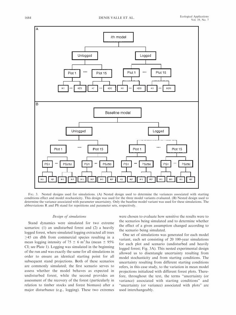
One set of simulations was generated for each model

variant, each set consisting of 20 100-year simulations

for each plot and scenario (undisturbed and heavily

logged forest; Fig. 3A). This nested experimental design

allowed us to disentangle uncertainty resulting from

model stochasticity and from starting conditions. The

uncertainty resulting from different starting conditions

refers, in this case study, to the variation in mean model

projections initialized with different forest plots. There-

fore, throughout the text, the terms ‘‘uncertainty (or

variance) associated with starting conditions’’ and

‘‘uncertainty (or variance) associated with plots’’ are

used interchangeably.

FIG. 3. Nested designs used for simulations. (A) Nested design used to determine the variances associated with startingconditions effect and model stochasticity. This design was used for the three model variants evaluated. (B) Nested design used todetermine the variance associated with parameter uncertainty. Only the baseline model variant was used for these simulations. Theabbreviations R and PS stand for repetitions and parameter sets, respectively.


One extra set of simulations was run solely to

determine uncertainty associated with parameter esti-

mation, consisting of 500 100-year simulations for each

plot and scenario. Parameters of the growth, recruit-

ment, and mortality submodels were drawn randomly

every two repetitions and were kept constant throughout

the run, resulting in a nested experimental design

(individual runs nested within parameter sets nested

within plots; Fig. 3B). This allowed us to separate the

uncertainty associated with parameter estimation from

the uncertainty resulting from model stochasticity and

from starting conditions.

Data analysis

Let L ¼ fS1, . . . , Smg be a finite set of model

alternatives, x be the data, and y be the response

variable. Furthermore, let li and r2i be the expected

value and the variance, respectively, of the response

variable given the data and the ith model alternative

(i.e., li ¼ E( y j x, Si ) and r2i ¼ Var( y j x, Si )). Let the

probability of the ith model given the data be pi (i.e., pi¼P(Si j x)). Draper (1995) showed that

Varðy j x; LÞ ¼Xm

i¼1

pir2i þ

Xm

i¼1

piðli � lÞ2

where

l ¼ Eðy j x; LÞ ¼Xm

i¼1

pili:

In other words, the variance of the response variable is

the sum of the within-model variance and the between-

model variance, both weighted by the probability of

each model given the data.

Following similar arguments, it can be shown that

Varð y j x; LÞ ¼Xm

i¼1

pir2y;i þ

Xm

i¼1

piðli � lÞ2

where r2y;i is the variance of the mean of the ith model

alternative. This equation can be further expanded by

decomposing r2y;i into the variances of the mean

associated with different uncertainty sources, such as

the variance of the mean associated with model stochas-

ticity, with starting conditions, and with parameter

uncertainty (r2y;ms;i, r2

y;p;i, and r2y;pu;i, respectively). If

model variants are created by adding or removing

assumptions from a single model, the uncertainty that

arises from the use of alternatemodeling assumptions can

be defined as the variance between these model variants,

given by

Xm

i¼1

piðli � lÞ2:

Therefore, the key equation that allows the partitioning of

the overall variance of the mean into different sources of

uncertainty is given by

Varð y j x; LÞ ¼Xm

i¼1

pi r2y;ms;i þ r2

y;p;i þ r2y;pu;i

� �

þXm

i¼1

piðli � lÞ2: ð1Þ

To illustrate, we could estimate some variable of

interest y with three independent climate models. If ywas mean annual temperature (8C), for example, li and

r2y;i would be the expected annual temperature and the

variance of the mean annual temperature, respectively,

as predicted by model i. Assume we populate the vector

li and r2y;i with model estimates so that we have li¼ [25,

22, 28] and r2y;i ¼ r2

y;ms;i þ r2y;p;i þ r2

y;pu;i ¼ [0.2, 0.2, 0.1]þ[0.4, 0.2, 0.1]þ [0.4, 0.1, 0.1]¼ [1, 0.5, 0.3], where vectors

are ordered from model 1 to model 3. Suppose the

probability of each model given the data was estimated

to be pi ¼ [0.2, 0.1, 0.7]. This implies that

l ¼Xm

i¼1

pili ¼ ½0:2; 0:1; 0:7�25

22

28

24

35 ¼ 26:8:

The variance of the mean annual temperature, taking

into account all three climate models, would therefore be

equal to

Varð y j x; LÞ ¼½0:2; 0:1; 0:7�1

0:5

0:3

264

375

þ ð½25; 22; 28� � ½26:8; 26:8; 26:8�Þ

3

0:2 0 0

0 0:1 0

0 0 0:7

264

375

25

22

28

264

375�

26:8

26:8

26:8

264

375

0B@

1CA

¼ 4:42:

A similar calculation could also be performed if the

modeler was interested in temporal variability (e.g., the

variable of interest y could then be the within-year

temperature range).

The elements of the within-model variance of the

mean (r2y;ms;i, r2

y;p;i, and r2y;pu;i) in Eq. 1 can be estimated

in several ways. In this paper, we chose to estimate

r2y;ms;i, r2

y;p;i, and r2y;pu;i by running the simulations

following a balanced nested experimental design and

using a variance component analysis assuming normal

residuals. These variances were then converted to r2y;ms;i,

r2y;p;i, and r2

y;pu;i, respectively, by dividing by the

appropriate number of observations. The variances

associated with starting conditions and with model

stochasticity (r2y;p;i and r2

y;ms;i, respectively) were deter-

mined using the expected means squares from an

ANOVA with one random effect (Table 2) estimated

at every 10-year time step. Using the simulation set in

which parameters were allowed to vary, the uncertainty

associated with parameter estimation (r2y;pu;i) was

determined using the variance components analysis

summarized in Table 3, also estimated separately for


every 10-year time step. The variance associated with

parameter uncertainty was the only result used from this

set of simulations. Because of the computational cost

necessary to determine r2y;pu;i for all models and since we

were interested in the magnitude and not the exact value

of this parameter, r2y;pu;i was determined only for the

baselinemodel and assumed to be the same for all models.

The probability of each model given the data (pi ) can

be estimated using Bayes rule. For instance, if there are

two independent data sets (e.g., Dmort and Drcrt, the

mortality and recruitment data sets, respectively), the

probability of model 1 given these two independent data

sets would be

pðM1 jDmort; DrcrtÞ

¼ LðDmort jM1Þ3 LðDrcrt jM1Þ3 pðM1ÞXm

i¼1

LðDmort jMiÞ3 LðDrcrt jMiÞ3 pðMiÞ

where L is the likelihood, and p(Mi ) and p(Mi jDmort,

Drcrt) are the prior and posterior probabilities, respec-

tively, of model Mi. Equal priors were assigned to each

model (i.e., p(Mi ) ¼ 1/3). The likelihood of each data

set given each model i, L(Dmort jMi ), and L(Drcrt jMi ),

was determined for each data set using SYMFOR’s

equations and inserting random effects to circumvent

the lack of independence of individual observations (as

described in Appendix B).

RESULTS

The results were in general consistent for the unlogged

and the logged scenarios. The 95% CIs describing the

uncertainty around the average projection from each

model variant tended to remain relatively constant and

small (Fig. 4A, B), and the variance of the mean was

mainly dominated by the effect of starting conditions

(Fig. 5A, B). A comparison of the projections from the

individual model variants, however, revealed that they

tended to diverge with increasing simulation length (Fig.

4A, B) and, as a consequence, after 100 years of

simulation, most 95% CIs did not overlap. These results

highlight the fact that, by neglecting simulation results

that could have originated had a different set of

assumptions been chosen, users of model projections

based on a single model variant tend to underestimate

the uncertainty associated with these projections. For

instance, users of the equilibrium model variant would

have predicted that basal area would recover to pre-

logging levels 50–70 years after logging, ignoring that, in

the absence of the dynamic equilibrium assumption, the

model (i.e., the baseline model variant) would predict

complete recovery of the basal area after 20–30 years.

Similarly, equilibrium model users would have predicted

an increase of the original basal after 100 years in the

unlogged scenario of 14–20% while the model without

this assumption (i.e., the baseline model variant) would

predict an increase of 26–32%.

As is often done in climate models, the overall trend

was initially described using a simple multimodel

average (i.e., equal weights are assigned to each model).

As simulation length increased, the width of the 95% CI

around the simple multimodel mean increased, reflecting

TABLE 2. ANOVA used to determine the variances associatedwith plots and model stochasticity (r2

y;p;i and r2y;ms;i,

respectively).

Source ofvariation df Expected MS

Plot np � 1 r2y;ms;i þ nrpsr2

y;p;i

Error np 3 (nrps � 1) r2y;ms;i

Total np 3 nrps � 1

Notes: These variances were estimated separately for eachmodel variant (i.e., baseline, dynamic equilibrium assumption,and growth extrapolation assumption models), logging sce-nario (logged and unlogged forest), and 10-year time step.This analysis corresponds to nested design shown in Fig. 3A.The variances r2

y;ms;i and r2y;p;i are associated with model

stochasticity and with plots (i.e., with different startingconditions), respectively, for the ith model; np and nrps arethe number of plots (i.e., 15) and number of repetitions perplot (i.e., 20), respectively.

TABLE 3. ANOVA used to determine the variance associated with parameter uncertainty(r2

y;pu;i) for the baseline model variant.

Source of variation df Expected MS

Plot np � 1 r2y;ms;i þ nrpsr2

y;pu;i þ nrpsnpsr2y;p;i

Parameter uncertainty np 3 (nps � 1) r2y;ms;i þ nrpsr2

y;pu;i

Model stochasticity np 3 nps 3 (nrps � 1) r2y;ms;i

Total np 3 nps 3 nrps � 1

Notes: The variances r2y;ms;i, r2

y;pu;i, and r2y;p;i were estimated separately for each logging

scenario (logged and unlogged forest), and 10-year time step. This analysis corresponds to thenested design shown in Fig. 3B. The variances r2

y;p;i, r2y;pu;i, and r2

y;ms;i are associated with plots(i.e., with different starting conditions), with parameter uncertainty, and with modelstochasticity, respectively, for the ith model; np, nrps, and nps are the number of plots (i.e.,15), the number of repetitions per parameter set (i.e., 2), and the number of randomly drawnparameter sets per plot (i.e., 250), respectively.


the divergence of results from the individual model

variants (Fig. 4C, D). The variance of the mean for the

simple multimodel average after 100 years was 21- and

29-fold larger than the average variance of the mean

from the individual model variants (for the unlogged

and logged scenarios, respectively). As shown in Fig.

5C, D, the uncertainty around the mean from the simple

multimodel average was dominated by the uncertainty

that arises from the use of the adopted assumptions.

More specifically, the variance of the mean associated

with the adopted assumptions represented 95% and 97%

of the overall variance of the mean, for the unlogged and

logged simulation results after 100 years, respectively.

These results, however, ignore the fact that some of

the model variants are more consistent with the data

than others. When using the data to estimate model

probabilities, it became clear that the equilibrium model

strongly conflicted with the data (i.e., the posterior

probability associated with this model was approxi-

mately zero) whereas the growthextrap and the baseline

models were equally supported by the data (Table 4).

This was not unexpected since the growthextrap and the

baseline model variants differed only in relation to the

growth submodel and the available growth data did not

distinguish between these two models. As a consequence

of the low weight of the equilibrium model, the variance

of the mean (at year 100) for the weighted multimodel

average (where the weights were estimated from the

data) was ;13–28% of those values when equal prob-

abilities were used (Fig. 5E, F; note narrower 95% CI in

Fig. 4E, F). The practical implication of these results is

that by using the weighted multimodel projections,

forest managers would expect that the forest would

recover its original basal area within 20–30 years after

logging vs. 20–80 years if a simple multimodel average

(i.e., equal weights) had been used. Likewise, the

projected increase in basal area after 100 years for the

unlogged forest with the weighted multimodel average is

equal to 26–36% of the basal area in year 0 vs. 13–40%

with the simple multimodel average. Despite the use of

FIG. 4. Mean model projections (and their associated 95% CIs) showing forest dynamics for an unlogged and a logged forest.Results from (A, B) the individual model variants (the baseline, dynamic equilibrium assumption, and growth extrapolationassumption models), (C, D) the simple multimodel average (i.e., equal model probabilities are assigned to each model variant), and(E, F) the weighted multimodel average (i.e., model probabilities are estimated from the data) are contrasted. The simplemultimodel average (C, D) incorporates the uncertainty associated with the contrasting mean results from the individual modelvariants (A, B) but ignores the negligible probability, given the data, associated with the dynamic equilibrium model variant. Theweighted multimodel average (E, F) takes the probability of each model variant into account, which results in a narrowerconfidence interval when compared to the simple multimodel average (C, D).


the data to estimate model probabilities and the

corresponding decrease in overall uncertainty, modeling

assumptions were still the greatest source of uncertainty

(Fig. 5E, F). The variance of the mean associated with

the used assumptions corresponded to 66% and 89% of

the overall variance of the mean, for the unlogged and

logged simulation results after 100 years, respectively.

DISCUSSION

Multimodel projections

Simulation model projections are frequently perceived

by modelers as conditional on the assumptions embed-

ded in the construction of the model (Haefner 1996).

Users of model projections, in contrast, are likely to

overlook this fact. In fact, it is impossible to assess the

uncertainty associated with these assumptions if projec-

tions are based on a single model variant. Multimodel

FIG. 5. Variance of the mean for the overall basal area projections, partitioned between parameter uncertainty, startingconditions effect, model stochasticity, and assumptions effect. Results are shown separately for logged and unlogged simulations.Results from (A, B) the individual model variants (variances were averaged over the three model variants), (C, D) the simplemultimodel average (i.e., equal model probabilities are assigned to each model variant), and (E, F) the weighted multimodelaverage (i.e., model probabilities are estimated from data) are contrasted. The individual model variants (A, B) exhibit anexcessively small mean overall variance of the mean that does not account for the uncertainties associated with model structure.Model structure uncertainty, shown as ‘‘Assumptions effect’’ (open bars), is taken into account in the simple multimodel average(C, D) and the weighted multimodel average (E, F), but the simple multimodel average assumes all models are equally likely whilethe weighted multimodel average effectively excludes the equilibrium model variant since this model variant has a negligibleprobability given the data.

TABLE 4. Posterior probability of each model variant (i.e.,baseline, growth extrapolation assumption [growthextrap],and dynamic equilibrium assumption [equilibrium] models)given the recruitment data, the mortality data, and both datasets combined.

Modelvariant

Recruitmentdata

Mortalitydata

Bothdata setscombined

Baseline 0.5 0.33 0.5Growthextrap 0.5 0.33 0.5Equilibrium 0.0 0.33 0.0

Notes: The posterior probability was estimated with Bayes’theorem by combining the prior probability (each model had anequal prior probability, one-third) and the likelihood (estimatedusing WinBUGS; see Appendix B). Recruitment and mortalitydata came from logged and unlogged forests (at km 67 and km114 at the Tapajos National Forest, Para, Brazil).


projections, on the other hand, are a multiple working

hypothesis (Chamberlin 1965) approach. The case study

illustrated that multimodel projections, even when based

on variants of a single model, can help mitigate this

problem by quantifying and including the uncertaintythat arises from the use of modeling assumptions,

particularly because these assumptions can be the

greatest source of uncertainty (e.g., Fig. 5C–F). The

effect of alternative model assumptions has been eval-

uated elsewhere (e.g., Chambers et al. 2004, Cropperand Loudermilk 2006), and this effect has been

compared to the uncertainty from other sources using

an approach based on sensitivity analysis (e.g., Knorr

and Heimann 2001, Jung et al. 2007). However, to ourknowledge, the comparison of the magnitude of

uncertainty from different sources has never been done

in a statistically comprehensive way. The case study also

exemplified that multimodel averaged projections can be

substantially different from projections based on a singlemodel variant (Fig. 4C–F vs. Fig. 4A, B).

Users and modelers may assume that even if

simulations are biased, the comparison of different

scenarios (e.g., logged vs. unlogged forest) or manage-

ment strategies simulated with the same set of assump-

tions would generally be unbiased (e.g., Ellner andFieberg 2003, Phillips et al. 2003, Arets 2005). The case

study results, however, show that this is not always true

given that the assumption effect may depend on the

scenario being simulated (e.g., compare baseline andequilibrium model projections in Fig. 4A vs. 4B).

The use of the best model, as chosen from a model

selection procedure, is equivalent to using a multimodel

projection in which the best model has a probability of

one and all the other alternative models have zero

probability. If all the other alternative models have

indeed zero probability, the use of the best model instead

of multimodel projections is clearly advantageous since

it reduces the number of simulations to be performed. If,

however, some of the other alternative models have a

nonzero probability (e.g., have similar fits to the data),then the use of the best model might be worrisome as the

best model may have wildly different predictions in

relation to other potential models when extrapolated.

Many ecological models are built for the purpose of

extrapolation (e.g., to predict the future) and, assumingthere is a set of plausible models that have similar fits to

the data, multimodel projections are essential to avoid

underestimating the uncertainty on model predictions.

The use of multimodel inference could have, for

instance, prevented such dramatic events as the disasterof the U.S. space shuttle Challenger. In this example,

engineers and managers had to predict the probability of

failure of the O-rings for a temperature that was outside

the range for which these rings had been previously

tested. A multimodel inference on the probability offailure of the O-rings for the low temperature at the time

of launching could have indicated the unacceptably high

risk associated with the space shuttle launching (Draper

1995).

Simple vs. weighted multimodel averaging

The case study suggests that simple multimodel

averaging, as often used with global vegetation and

climate models (Cramer et al. 2001, Koster et al. 2004),

might result in an overestimation of variability (similarto results in Murphy et al. [2004]). Indeed, multiple

models (or model variants) can be created based on

many biologically reasonable alternatives representing a

given phenomenon. For instance, to avoid trees from

getting too large, a forest modeler might use an equation

PLATE 1. (Left) A mixed tropical forest in the Brazilian Amazon. (Right) Logs of a tropical tree species at a sawmill in theBrazilian Amazon. The person standing close to the logs is approximately 1.75 m tall. Photo credits: forest, C. L. Staudhammer;logs, Simone Bauch.


that predicts zero growth for large trees (e.g., Alder and

Silva 2000, Gourlet-Fleury and Houllier 2000, Kamme-

sheidt et al. 2001, Kohler et al. 2003) or increase the

mortality rate of large trees as a result of senescence

(e.g., Phillips et al. 2003, 2004, Chambers et al. 2004,

Valle et al. 2007). Similarly, the dynamic equilibrium

assumption can be implemented by fine tuning the

model (e.g., Phillips et al. 2004, Gourlet-Fleury et al.

2005, Valle et al. 2007) or by replacing every tree that

dies by a newly recruited tree (e.g., Chambers et al.

2004). To reduce the uncertainty that arises from the use

of assumptions and consequently reduce overall uncer-

tainty around the mean, it is crucial to evaluate which of

these alternative representations are more consistent

with the data and weight them accordingly. Multimodel

projection, in which the individual models are weighted

according to their past performance, has been shown

elsewhere to result in a higher prediction ability than

individual models and simple multimodel averages

(Krishnamurti et al. 1999).

Even if the available data do not help to discern

between these alternative representations, the acknowl-

edgment of this fact can guide researchers to conduct

experiments or collect observational data in order to

strategically reduce model structure uncertainty. In the

case study, despite the fact that model parameters were

carefully fine tuned within the confidence interval of

each parameter, the equilibrium model was shown to be

inconsistent with the data. On the other hand, the data

supported equally well model variants that only differed

in relation to how growth submodel extrapolations were

handled (e.g., baseline and growthextrap models). A

carefully designed experiment might have helped to

further discern between the baseline and the growthex-

trap models.

General applicability of the uncertainty

partitioning methodology

It has been illustrated how a balanced, nested

simulation design facilitates in partitioning the within-

model variance into various sources of uncertainty and

how multimodel projections allow estimation of uncer-

tainty that arises as a result of the use of different model

assumptions (between model variance). This method can

potentially be applied to other types of simulation

models since the sources of uncertainty analyzed here

(i.e., parameter uncertainty, model stochasticity, effect

of starting conditions, and uncertainty associated with

model assumptions) are likely to be jointly present in

other models as well. This method might help model

developers and users to identify which are the greatest

sources of uncertainty and, more importantly, which

type of data should be collected or experiment

conducted to decrease the uncertainty from these

sources. However, depending on the computational

power needed for a single run of some models (e.g.,

global biogeochemical/biosphere models), the numerous

simulations needed for this methodology might limit its

use. One could reduce the number of simulations by

eliminating part of the nested simulation design at the

cost of additional assumptions in the data analysis. For

instance, in the case study described above, parameter

estimation uncertainty could have been assessed for only

one plot and one model and assumed to be the same for

all other plots and models. Also, simulations might

eventually become too numerous when using this

method if too many modeling assumptions are analyzed.

The number of simulations can be somewhat reduced by

discarding those modeling assumptions that are not

supported by the data; however, modelers, and poten-

tially other stakeholders, will ultimately have to decide

which are the key modeling assumptions that should be

included in their uncertainty analysis.

Simulation models have and will increasingly be used

to predict the outcomes of direct or indirect human-

induced changes (e.g., logging, burning, fragmentation,

or carbon accumulation in the atmosphere), sometimes

with millennium-long time windows (e.g., Chambers et

al. 2001). The uncertainty associated with these model

projections is underestimated, however, if the uncertain-

ty resulting from assumptions used in model building is

not taken into account. This has the potential to mislead

decision makers, reduce public confidence in model

projections, hamper the ability to anticipate extreme

events and devise robust policies, and could potentially

have dire consequences (Clark et al. 2001, Pielke and

Conant 2003). Simulation modelers in ecology should

follow the lead of those in the field of statistics, taking

model structure uncertainty into account through multi-

model projections.

ACKNOWLEDGMENTS

We are very thankful to Ben Bolker for his numerousinsightful comments. We also thank Linda Young and JackPutz for discussion and comments on the thesis that gave originto this paper, and Paulo M. Brando and Pieter Zuidema forreviewing an earlier version of this article. Funding for DenisValle was provided by University of Florida.

LITERATURE CITED

Alder, D., and J. N. M. Silva. 2000. An empirical cohort modelfor management of Terra Firme forests in the BrazilianAmazon. Forest Ecology and Management 130:141–157.

Arets, E. J. M. M. 2005. Long-term responses of populationsand communities of trees to selective logging in tropical rainforests in Guyana. Tropenbos International, Georgetown,Guyana.

Bradshaw, C. J. A., Y. Fukuda, M. Letnic, and B. W. Brook.2006. Incorporating known sources of uncertainty todetermine precautionary harvests of saltwater crocodiles.Ecological Applications 16:1436–1448.

Brown, J. H., J. F. Gillooly, A. P. Allen, V. M. Savage, andG. B. West. 2004. Toward a metabolic theory of ecology.Ecology 85:1771–1789.

Burnham, K. P., and D. R. Anderson. 1998. Model selectionand inference: a practical information-theoretic approach.Springer, New York, New York, USA.

Carpenter, S. R. 2002. Ecological futures: building an ecologyof the long now. Ecology 83:2069–2083.

Chamberlin, T. C. 1965. The method of multiple workinghypotheses. Science 148:754–759.


Chambers, J. Q., N. Higuchi, L. M. Teixeira, J. Santos, S. G.Laurance, and S. E. Trumbore. 2004. Response of treebiomass and wood litter to disturbance in a Central AmazonForest. Oecologia 141:596–611.

Chambers, J. Q., N. Higuchi, E. S. Tribuzy, and S. E.Trumbore. 2001. Carbon sink for a century. Nature 410:429.

Chatfield, C. 1995. Model uncertainty, data mining andstatistical inference. Journal of the Royal Statistical Society,Series A 158:419–466.

Clark, J. S., et al. 2001. Ecological forecasts: an emergingimperative. Science 293:657–660.

Coomes, D. A., R. P. Duncan, R. B. Allen, and J. Truscott.2003. Disturbances prevent stem size-density distributions innatural forests from following scaling relationships. EcologyLetters 6:980–989.

Cox, P. M., P. P. Harris, C. Huntingford, R. A. Betts, M.Collins, C. D. Jones, T. E. Jupp, J. A. Marengo, and C. A.Nobre. 2008. Increasing risk of Amazonian drought due todecreasing aerosol pollution. Nature 453:212–216.

Cramer, W., et al. 1999. Comparing global models of terrestrialnet primary productivity (NPP): overview and key results.Global Change Biology 5:1–15.

Cramer, W., et al. 2001. Global response of terrestrialecosystem structure and function to CO2 and climate change:results from six dynamic global vegetation models. GlobalChange Biology 7:357–373.

Cropper, W. P., Jr., and E. L. Loudermilk. 2006. Theinteraction of seedling density dependence and fire in amatrix population model of longleaf pine (Pinus palustris).Ecological Modelling 198:487–494.

DeFries, R. S., J. A. Foley, and G. P. Asner. 2004. Land-usechoices: balancing human needs and ecosystem function.Frontiers in Ecology and the Environment 2:249–257.

Degen, B., L. Blanc, H. Caron, L. Maggia, A. Kremer, and S.Gourlet-Fleury. 2006. Impact of selective logging on geneticcomposition and demographic structure of four tropical treespecies. Biological Conservation 131:386–401.

Draper, D. 1995. Assessment and propagation of modeluncertainty. Journal of the Royal Statistical Society, SeriesB 57:45–97.

Elderd, B. D., V. M. Dukic, and G. Dwyer. 2006. Uncertaintyin predictions of disease spread and public health responsesto bioterrorism and emerging diseases. Proceedings of theNational Academy of Sciences (USA) 103:15693–15697.

Ellison, A. M. 2004. Bayesian inference in ecology. EcologyLetters 7:509–520.

Ellner, S. P., and J. Fieberg. 2003. Using PVA for managementdespite uncertainty: effects of habitat, hatcheries, and harveston salmon. Ecology 84:1359–1369.

Gertner, G., X. Cao, and H. Zhu. 1995. A quality assessment ofa Weibull based growth projection system. Forest Ecologyand Management 71:235–250.

Gourlet-Fleury, S., G. Cornu, S. Jesel, H. Dessard, J. G.Jourget, L. Blanc, and N. Picard. 2005. Using models topredict recovery and assess tree species vulnerability inlogged tropical forests: a case study from French Guiana.Forest Ecology and Management 209:69–86.

Gourlet-Fleury, S., and F. Houllier. 2000. Modelling diameterincrement in a lowland evergreen rain forest in FrenchGuiana. Forest Ecology and Management 131:269–289.

Haefner, J. W. 1996. Modeling biological systems: principlesand applications. Chapman and Hall, New York, New York,USA.

Hoeting, J. A., D. Madigan, A. E. Raftery, and C. T. Volinsky.1999. Bayesian model averaging: a tutorial. Statistical Science14:382–401.

Jung, M., et al. 2007. Uncertainties of modeling gross primaryproductivity over Europe: a systematic study on the effects ofusing different drivers and terrestrial biosphere models. GlobalBiogeochemical Cycles 21. [doi: 10.1029/2006GB002915]

Kammesheidt, L., P. Kohler, and A. Huth. 2001. Sustainabletimber harvesting in Venezuela: a modelling approach.Journal of Applied Ecology 38:756–770.

Knorr, W., and M. Heimann. 2001. Uncertainties in globalterrestrial biosphere modeling. 1. A comprehensive sensitivityanalysis with a new photosynthesis and energy balancescheme. Global Biogeochemical Cycles 15:207–225.

Kohler, P., J. Chave, B. Riera, and A. Huth. 2003. Simulatingthe long-term response of tropical wet forests to fragmenta-tion. Ecosystems 6:114–128.

Kohyama, T., E. Suzuki, T. Partomihardjo, T. Yamada, and T.Kubo. 2003. Tree species differentiation in growth, recruit-ment and allometry in relation to maximum height in aBornean mixed dipterocarp forest. Journal of Ecology 91:797–806.

Koster, R. D., et al. 2004. Regions of strong coupling betweensoil moisture and precipitation. Science 305:1138–1140.

Krishnamurti, T. N., C. M. Kishtawal, T. E. LaRow, D. R.Bachiochi, Z. Zhang, C. E. Williford, S. Gadgil, and S.Surendran. 1999. Improved weather and seasonal climateforecasts from multimodel superensemble. Science 285:1548–1550.

Link, W. A., and R. J. Barker. 2006. Model weights and thefoundations of multimodel inference. Ecology 87:2626–2635.

Malhi, Y., J. T. Roberts, R. A. Betts, T. J. Killeen, W. Li, andC. A. Nobre. 2008. Climate change, deforestation, and thefate of the Amazon. Science 319:169–172.

Malhi, Y., et al. 2004. The above-ground coarse woodproductivity of 104 neotropical forest plots. Global ChangeBiology 10:563–591.

Muller-Landau, H. C., et al. 2006. Comparing tropical foresttree size distributions with the predictions of metabolicecology and equilibrium models. Ecology Letters 9:589–602.

Murphy, J. M., D. M. H. Sexton, D. N. Barnett, G. S. Jones,M. J. Webb, M. Collins, and D. A. Stainforth. 2004.Quantification of modelling uncertainties in a large ensembleof climate change simulations. Nature 430:768–772.

Oliveira, L. C. 2005. Efeito da exploracao da madeira e dediferentes intensidades de desbastes sobre a dinamica davegetacao de uma area de 136 ha na Floresta Nacional doTapajos. Dissertation. Escola Superior de Agricultura ‘‘Luizde Queiroz’’/USP, Piracicaba, Brazil.

Pacala, S. W., C. D. Canham, J. Saponara, J. A. Silander, R. K.Kobe, and E. N. Ribbens. 1996. Forest models defined byfield-measurements: estimation, error analysis, and dynamics.Ecological Monographs 66:1–43.

Palace, M., M. Keller, and H. Silva. 2008. Necromassproduction: studies in undisturbed and logged Amazonforests. Ecological Applications 18:873–884.

Pascual, M., P. Kareiva, and R. Hilborn. 1997. The influence ofmodel structure on conclusions about the viability andharvesting of Serengeti wildebeest. Conservation Biology11:966–976.

Phillips, P. D., T. E. Brash, I. Yasman, P. Subagyo, and P. R.van Gardingen. 2003. An individual-based spatially explicittree growth model for forests in East Kalimantan (Indone-sian Borneo). Ecological Modelling 159:1–26.

Phillips, P. D., C. P. de Azevedo, B. Degen, I. S. Thompson,J. N. M. Silva, and P. R. van Gardingen. 2004. Anindividual-based spatially explicit simulation model forstrategic forest management planning in the eastern Amazon.Ecological Modelling 173:335–354.

Phillips, P. D., I. Yasman, T. E. Brash, and P. R. vanGardingen. 2002. Grouping tree species for analysis of forestdata in Kalimantan (Indonesian Borneo). Forest Ecologyand Management 157:205–216.

Pielke, R. A., Jr., and R. T. Conant. 2003. Best practices inprediction for decision-making: lessons from the atmosphericand earth sciences. Ecology 84:1351–1358.


Porte, A., and H. H. Bartelink. 2002. Modelling mixed forestgrowth: a review of models for forest management.Ecological Modelling 150:141–188.

Sheil, D., and R. M. May. 1996. Mortality and recruitment rateevaluations in heterogeneous tropical forests. Journal ofEcology 84:91–100.

Silva, J. N. M., J. O. P. Carvalho, J. C. A. Lopes, B. F.Almeida, D. H. M. Costa, L. C. Oliveira, J. K. Vanclay, andJ. P. Skovsgaard. 1995. Growth and yield of a tropical rain-forest in the Brazilian Amazon 13 years after logging. ForestEcology and Management 71:267–274.

Silva, J. N. M., J. O. P. Carvalho, J. C. A. Lopes, R. P. Oliveira,and L. C. Oliveira. 1996. Growth and yield studies in theTapajos region, Central Brazilian Amazon. CommonwealthForestry Review 75:325–329.

Stainforth, D. A., et al. 2005. Uncertainty in predictions of theclimate response to rising levels of greenhouse gases. Nature433:403–406.

Sutherland, W. J. 2001. Sustainable exploitation: a review ofprinciples and methods. Wildlife Biology 7:131–140.

Valle, D., P. Phillips, E. Vidal, M. Schulze, J. Grogan, M. Sales,and P. van Gardingen. 2007. Adaptation of a spatially

explicit individual tree-based growth and yield model andlong-term comparison between reduced-impact and conven-tional logging in eastern Amazonia, Brazil. Forest Ecologyand Management 243:187–198.

van Gardingen, P. R., M. J. McLeish, P. D. Phillips, D.Fadilah, G. Tyrie, and I. Yasman. 2003. Financial andecological analysis of management options for logged-overDipterocarp forests in Indonesian Borneo. Forest Ecologyand Management 183:1–29.

van Gardingen, P. R., D. R. Valle, and I. S. Thompson. 2006.Evaluation of yield regulation options for primary forest inTapajos National Forest, Brazil. Forest Ecology andManagement 231:184–195.

van Ulft, L. H. 2004. Regeneration in natural and loggedtropical rain forest. Tropenbos International, Georgetown,Guyana.

Wigley, T.M. L., and S. C. B. Raper. 2001. Interpretation of highprojections for global-mean warming. Science 293:451–454.

Wintle, B. A., M. A. McCarthy, C. T. Volinsky, and R. P.Kavanagh. 2003. The use of Bayesian model averaging tobetter represent uncertainty in ecological models. Conserva-tion Biology 17:1579–1590.

APPENDIX A

Parameters used for different model variants of SYMFOR (Ecological Archives A019-068-A1).

APPENDIX B

Estimating the likelihood of each data set given each model (Ecological Archives A019-068-A2).


the importance of multimodel projections to assess...

Documents