the increase in shaft capacity with time for friction
TRANSCRIPT

Louisiana State UniversityLSU Digital Commons
LSU Historical Dissertations and Theses Graduate School
1996
The Increase in Shaft Capacity With Time forFriction Piles Driven Into Saturated Clay.Hani Hasan TitiLouisiana State University and Agricultural & Mechanical College
Follow this and additional works at: https://digitalcommons.lsu.edu/gradschool_disstheses
This Dissertation is brought to you for free and open access by the Graduate School at LSU Digital Commons. It has been accepted for inclusion inLSU Historical Dissertations and Theses by an authorized administrator of LSU Digital Commons. For more information, please [email protected].
Recommended CitationTiti, Hani Hasan, "The Increase in Shaft Capacity With Time for Friction Piles Driven Into Saturated Clay." (1996). LSU HistoricalDissertations and Theses. 6313.https://digitalcommons.lsu.edu/gradschool_disstheses/6313

INFORMATION TO USERS
This manuscript has been reproduced from the microfilm master. UMI
films the text directly from the original or copy submitted. Thus, some
thesis and dissertation copies are in typewriter face, while others may be
from any type of computer printer.
The quality of this reproduction is dependent upon the quality of the
copy submitted. Broken or indistinct print, colored or poor quality
illustrations and photographs, print bleedthrough, substandard margins,
and improper alignment can adversely affect reproduction.
In the unlikely event that the author did not send UMI a complete
manuscript and there are missing pages, these will be noted. Also, if
unauthorized copyright material had to be removed, a note will indicate
the deletion.
Oversize materials (e.g., maps, drawings, charts) are reproduced by
sectioning the original, beginning at the upper left-hand comer and
continuing from left to right in equal sections with small overlaps. Each
original is also photographed in one exposure and is included in reduced
form at the back of the book.
Photographs included in the original manuscript have been reproduced
xerographically in this copy. Higher quality 6” x 9” black and white
photographic prints are available for any photographs or illustrations
appearing in this copy for an additional charge. Contact UMI directly to
order.
UMIA Bell & Howell Information Company
300 North Zeeb Road, Ann Aitoor MI 48106-1346 USA 313/761-4700 800/521-0600
Reproduced with permission of the copyright owner. Further reproduction prohibited without permission.

Reproduced with permission of the copyright owner. Further reproduction prohibited without permission.

THE INCREASE IN SHAFT CAPACITY W ITH TIME FOR FRICTION PILES DRIVEN INTO SATURATED CLAY
A Dissertation
Submitted to the Graduate Faculty of the Louisiana State University and
Agricultural and Mechanical College in partial fulfillment of the
requirements for the degree of Doctor of Philosophy
m
The Department of Civil and Environmental Engineering
byHani Hasan Titi
B.S.C.E., Yarmouk University, Irbid, Jordan, 1987 M.S.C.E., Jordan University of Science and Technology, Irbid, Jordan, 1990
December 1996
Reproduced with permission of the copyright owner. Further reproduction prohibited without permission.

UMI Number: 9712861
UMI Microform 9712861 Copyright 1997, by UMI Company. All rights reserved.
This microform edition is protected against unauthorized copying under Title 17, United States Code.
UMI300 North Zeeb Road Ann Arbor, MI 48103
Reproduced with permission of the copyright owner. Further reproduction prohibited without permission.

Dedicated
To M y Parents
ii
Reproduced with permission of the copyright owner. Further reproduction prohibited without permission.

ACKNOWLEDGEMENTS
I would like to express my deepest appreciation to my advisor Professor G. Wije
Wathugala for his friendship, guidance, and support throughout this research, project.
His comments and suggestions have been invaluable.
My sincere gratitude is extended to Professor George Z. Voyiadjis. His help
and support during my study is acknowledged. I would like to thank Professor
Mehmet T. Tumay. His help, valuable comments, and suggestions are acknowledged
with gratitude. My thanks also goes to Professor Roger K. Seals for his valuable
comments. I would like to thank Professor Bruce Sbarky for his serving in the
examination committee.
I would like here to remember the memory of Professor Yalcin B. Acar who was
a committee member. His friendship will always remain in my thoughts.
This research performed herein was partially supported by Louisiana Transporta
tion Research Center (LTRC) and by the National Science Foundation (NSF) through
the grant No. CMS-9410482. These supports are gratefully acknowledged.
My t h a n k s extended to Dr. Akram Alshawabkeh and to Mr. Surajit Pal for
their friendship and support. I would like also to thank Mr. Manaa’ Mesleh for his
friendship and support. The help of my friend Mr. Ibrahim Mansi is acknowledged
with appreciation. I would like to t h ank my parents and siblings for continuous
support and encouragements.
To my wife Eman and my daughter Miriam I owe the most. This work would
have not been possible without their support and love.
iii
Reproduced with permission of the copyright owner. Further reproduction prohibited without permission.

CONTENTS
D E D IC A T IO N ...................................................................................................... ii
A C K N O W L E D G E M E N T S............................................................................. iii
L IS T O F T A B L E S ..................................................................................................... vii
LIST OF F IG U R E S ................................................................................................ viii
ABSTRACT .............................................................. xvii
CHAPTER
1 INTRODUCTION ....................................................................................... 11.1 B ack g ro u n d .......................................................t .......................................... 11.2 Objectives and Scope of the R esearch....................................................... 31.3 Organization of the M an u sc rip t................................................................. 4
2 BACKGROUND .......................................................................................... 62.1 In troduction .................................................................................................... 62.2 Effects of Pile Driving on the Clay-Water S y s te m ................................ 7
2.2.1 Disturbance Effects on Soil P roperties .......................................... 82.2.2 Changes in Pore Water P re s s u re s ................................................. 82.2.3 Equalization of Pore Water Pressures and S tresses ................... 11
2.3 Pile S e tu p ........................................................................................................ 122.4 Soil Sensitivity .............................................................................................. 182.5 Methods of Predicting Pile Shaft C a p a c ity ............................................. 192.6 Pile-Setup Related S tu d ies .......................................................................... 21
3 HIERARCHICAL SINGLE SURFACE M ODELING APPROACH 263.1 In troduction .................................................................................................... 263.2 The 5*-Series of HiSS Constitutive M o d e ls ............................................. 27
3.2.1 Basics of the Incremental Theory of P la s t ic i ty .......................... 273.2.2 Yield Surface, F ................................................................................. 283.2.3 Hardening Function, O p , ................................................................. 323.2.4 Interpolation Functions.................................................................... 343.2.5 Potential Function, Q ....................................................................... 36
3.3 The Proposed Interface HiSS-^,- M odel.................................................... 363.3.1 Potential Function, Q ....................................................................... 373.3.2 Translation R u le ................................................................................. 39
3.4 Evaluation of the M o d e l ............................................................................. 443.4.1 Field Investigation on Sabine C la y ................................................. 44
iv
Reproduced with permission of the copyright owner. Further reproduction prohibited without permission.

3.4.2 Material Parameters ........................................................................ 453.4.3 Implementation of the Model into Computer Procedures . . . 483.4.4 Capabilities and Properties of the M o d e l .................................... 483.4.5 Calibration of the M o d e l ................................................................. 51
4 S IM U L A T IO N O F P IL E IN S T A L L A T IO N ............................................ 604.1 In troduction ..................................................................................................... 604.2 Methods of Pile Driving S im ulation ........................................................... 614.3 Strain Path M ethod........................................................................................ 63
4.3.1 Limitations ........................................................................................ 634.3.2 Closed-Ended P i l e s ........................................................................... 634.3.3 Open-Ended P ile s .............................................................................. 67
4.3.3.1 Ring S o u rc e ........................................................................ 704.3.3.2 Superposing a Uniform Steady Flow on the Source-
Ring F lo w ........................................................................... 714.3.3.3 Strain F i e l d ....................................................................... 73
4.4 Numerical Simulation of Pile D riv in g ........................................................ 78
5 V E R IF IC A T IO N : P IL E D R IV IN G , S U B S E Q U E N T C O N SO L ID A T IO N A N D P IL E LO AD T E S T S .............................................................. 845.1 In troduction ..................................................................................................... 845.2 Field Tests at Sabine Site ........................................................................... 85
5.2.1 Test P rocedures................................................................................. 855.2.2 Pile Segment M o d e ls ....................................................................... 885.2.3 Results of Field Experim ents.......................................................... 88
5.3 The Finite Element Program A B A Q U S/S tandard................................ 925.3.1 Analysis of Porous M ed ia ................................................................ 925.3.2 Implementation of the HiSS-£Jt- Model in A B A Q U S ................. 955.3.3 Finite Element M e s h ....................................................................... 96
5.4 Pile D riv in g ........................................................................................................1025.5 Consolidation and Pile Load T e s ts .................................................................1085.6 Pile S e tu p ...........................................................................................................135
6 N U M E R IC A L SIM U L A T IO N O F T H E B E H A V IO R O F C L O S E D -E N D E D P IL E S .....................................................................................................1376.1 In troduction ....................................................................................................... 1376.2 Field Experim ents..............................................................................................1386.3 Finite Element M e s h ....................................................................................... 1386.4 Pile D r iv in g ....................................................................................................... 1436.5 Consolidation and Pile Load T e s ts ................................................................ 1486.6 Pile S e tu p ...........................................................................................................167
7 N U M E R IC A L S IM U L A T IO N O F T H E B E H A V IO R O F O P E N -E N D E D P IL E S .....................................................................................................1697.1 In troduction ....................................................................................................... 169
v
Reproduced with permission of the copyright owner. Further reproduction prohibited without permission.

7.2 Field Experim ents............................................................................................. 1707.3 Finite Element M esh ........................................................................................1707.4 Pile D r iv in g .......................................................................................................178
7.4.1 The 3 in. x 0.125 in. Open-ended Pile Segment Model . . . . 1797.4.2 The 3 in. x 0.065 in. Open-ended Pile Segment Model . . . . 179
7.5 Consolidation and Pile Load T e s ts ................................................................ 1847.5.1 The 3 in. x 0.125 in. Open-ended Pile Segment Model . . . . 1847.5.2 The 3 in. x 0.065 in. Open-ended Pile Segment Model . . . . 204
7.6 Pile S e t u p ..........................................................................................................204
8 NUMERICAL EXPERIMENTS ON A FULL-SCALE CLOSED- ENDED P I L E .................................................................................................. 2078.1 In troduction ...................................................................................................... 2078.2 Pile C haracteristics......................................................................................... 2078.3 Simulation of Pile D r iv in g .............................................................................2098.4 Consolidation and Pile Load T e s ts ................................................................2098.5 Pile S e tu p ......................................................................................................... 213
9 SUMMARY, CONCLUSIONS, AND RECOMMENDATIONS . 2189.1 Summary ......................................................................................................... 2189.2 C onclusions...................................................................................................... 2199.3 Recommendations............................................................................................ 220
R E FE R E N C E S........................................................................................................ 222
A PPEN D IX A: PILE SETUP RELATED ST U D IE S............................234
A PPEN D IX B: NUMERICAL SIMULATION OF THE BEHAVIOR OF 3 in. x 0.065 in. O PEN -ENDED PILE SEGMENT MODEL ....................................................... 242
V I T A ........................................................................................................................... 253
VI
Reproduced with permission of the copyright owner. Further reproduction prohibited without permission.

LIST OF TABLES
3.1 Soil properties of normally consolidated Sabine clay (after Bogard and Matlock, 1979, and Earth Technology Corporation, 1986)...................... 46
3.2 Material constants for Sabine clay (after Wathugala, 1990).................... 47
5.1 Dimensions of the pile segment models used in the field experiments. 86
A .l Pile setup related studies ............................................................................... 235
vii
Reproduced with permission of the copyright owner. Further reproduction prohibited without permission.

LIST OF FIGURES2.1 Full scale field data on bearing capacity increase with time of friction
piles driven into c la y ...................................................................................... 14
2.2 Dissipation of pore water pressure during soil consolidation aroundthe Piezo-Lateral Stress cell in Empire clay (after Azzouz, 1986). . . 16
2.3 Decrease in bearing capacity with time after driving friction piles intoc l a y . .................................................................................................................. 17
2.4 Comparison of measured increase in bearing capacity of pile with theoretical increase in strength of soil adjacent to (a) Pile driven into Drammen clay, (b) Pile driven into San Francisco Bay mud (after Randolph et al., 1979)...................................................................................... 23
2.5 Results of static tension load tests conducted on a 3 in. x 0.125 in.open-ended pile segment model at Sabine Pass, Texas (after Earth Technology Corp., 1986).................................................................................. 25
3.1 Shape of the yield surface in the Ji-y/JiD space...................................... 30
3.2 (a) Shape of the yield surface in the triaxial plane; (b) Trace of theyield surface in the octahedral plane............................................................ 31
3.3 The yield surface, F, and the reference surface, R, in the triaxial plane. 33
3.4 Results of direct simple shear test on NC Boston Blue Clay, (a) Stresspath; (b) Shear stress-strain and pore water pressure-strain curves (after Ahmad, 1990)......................................................................................... 38
3.5 Location of the translation tensor, ay, in the J \-y /J m space (after Wathugala, 1990).............................................................................................. 40
3.6 Location of the translation tensor, ay; section A-A in the octahedral plane (after Wathugala, 1990)........................................................................ 43
3.7 (a) Comparison of predicted effective stress paths during undrainedtriaxial compression test using and models; (b) The corresponding predicted stress-strain relationships...................................................... 49
3.8 (a) Variation of predicted effective stress path during undrained triaxial compression test with Aq\ (b) The corresponding predicted stress- strain relationships........................................................................................... 50
3.9 (a) Variation of predicted effective stress path during simple shear testwith A q; (b) The corresponding predicted stress-strain relationships. . 52
viii
Reproduced with permission of the copyright owner. Further reproduction prohibited without permission.

3.10 Comparison of predicted and measured effective radial stresses immediately after driving 1.72 in. diameter pile segment model into Sabine clay...................................................................................................... 53
3.11 Comparison of predicted and measured effective radial stresses immediately after driving 3 in. diameter pile segment model into Sabine clay ................................................................................................................... 54
3.12 (a) Variation of effective stress patb with A, during pile driving aspredicted by the model, using strain path method; (b) The corresponding predicted stress-strain relationships.......................................... 56
3.13 Predicted distribution of effective radial stress for different A, values immediately after pile driving, using the model................................. 57
3.14 Predicted distribution of pore water pressure for different Aq values immediately after pile driving, using the * u model................................ 58
4.1 Geometry of the simple pile........................................................................... 65
4.2 Strain field around simple pile for (a) Soil element located initially atra = R, (b) Soil element located initially at r„ = 2R ................................ 68
4.3 Distribution of strains immediately after driving at a depth z = R. . . 69
4.4 Geometry of the open-ended pile................................................................. 72
4.5 The effect of pile driving velocity, U, on the strain field of the surrounding soil (soil element is located at radial distance r = 1.5i2). . . 76
4.6 Strain field predicted by SPM due to an open-ended pile driving; (a)Soil element outside the pile located finally at radial distance r / =1.5f2, (b) Soil element inside the pile located finally at radial distanceTf = 15f............................................................................................................... 77
4.7 Strain paths, in the deviatoric space, of soil elements located at theimmediate vicinity outside and inside the wall during open-ended pile driving; (a) Ei vs E2] (b) E3 vs E2.............................................................. 79
4.8 The predicted effective stress path for a soil element at the pile-soilinterface path during pile driving................................................................. 81
4.9 Predicted distribution of effective stresses immediately after pile driving. 82
4.10 Predicted distribution of pore water pressure immediately after pile driving............................................................................................................... 83
5.1 The test procedure sequence for the field experiments........................... 87
ix
Reproduced with permission of the copyright owner. Further reproduction prohibited without permission.

5.2 The 1.72 in. diameter pile segment model (after Earth TechnologyCorp., 1986)....................................................................................................... 89
5.3 The 3 in. diameter pile segment model (after Earth Technology Corp.,1986).................................................................................................................... 90
5.4 Variations of the measured pressures during soil consolidation aroundthe 1.72 in. diameter pile segment model (after Earth Technology Corp., 1986)....................................................................................................... 91
5.5 Results of the field static tension tests conducted on the 1.72 in. diameter pile segment model (after Earth Technology Corp., 1986). . . 93
5.6 Diagram for the use of UMAT in the finite element analysis................. 97
5.7 ABAQUS axisymmetric solid element CAX8RP used in the finite element analysis................................................................................................... 98
5.8 The finite element mesh used to discretize the soil domain around the1.72 in diameter pile segment model..............................................................100
5.9 Variation with radial distance of predicted effective stress paths duringpile driving for soil elements located 16 m below the ground surface. . 101
5.10 Predicted effective stress path for a soil element at the soil-pile interface during driving the 1.72 in. diameter pile segment model. . . 103
5.11 Predicted distribution of effective stresses at 16 m below the ground surface immediately after driving 1.72 in. diameter pile segment model. 104
5.12 Comparison of predicted and measured effective radial stresses duringsoil consolidation around the 1.72 in. diameter pile segment model. . 106
5.13 Predicted distribution of pore water pressure immediately after driving 1.72 in. diameter pile segment model.....................................................107
5.14 Sequence of the load tests conducted during soil consolidation aroundthe 1.72 in. diameter pile segment model.....................................................109
5.15 Comparison of predicted and measured normalized excess pore waterpressures during soil consolidation around the 1.72 in. diameter pile segment model....................................................................................................I l l
5.16 Predicted dissipation of pore water pressures during soil consolidationaround the 1.72 in. diameter pile segment model.......................................112
5.17 Predicted increase in effective radial stresses during the consolidationof the soil around the 1.72 in. diameter pile segment model....................113
x
Reproduced with permission of the copyright owner. Further reproduction prohibited without permission.

5.18 Predicted distribution of effective stress at a depth of 16 m at the end of soil consolidation around the 1.72 in. diameter pile segment model....................................................................................................................114
5.19 Predicted effective stress path for a soil element at the pile-soil interface during driving and consolidation of the soil around the 1.72in. diameter pile segment model.................................................................... 116
5.20 Comparison of predicted and measured response during pile load test# 1 conducted on the 1.72 in. diameter pile segment model...........117
5.21 Comparison of predicted and measured response during pile load test# 2 conducted on the 1.72 in. diameter pile segment model...........119
5.22 Comparison of predicted and measured response during pile load test# 3 conducted on the 1.72 in. diameter pile segment model...................121
5.23 Comparison of predicted and measured response during pile load test# 4 conducted on the 1.72 in. diameter pile segment model...................123
5.24 Comparison of predicted and measured response during pile load test# 5 conducted on the 1.72 in. diameter pile segment model...................125
5.25 Comparison of predicted and measured response during pile load test# 6 conducted on the 1.72 in. diameter pile segment model...................127
5.26 Comparison of predicted and measured response during pile load test# 7 conducted on the 1.72 in. diameter pile segment model...................130
5.27 Comparison of predicted and measured response (shear transfer vs displacement) during the final cyclic pile load test conducted on the1.72 in. diameter pile segment model.......................................................... 132
5.28 Comparison of predicted and measured response (shear transfer vs time) during the final cyclic pile load test conducted on the 1.72 in. diameter pile segment model...........................................................................133
5.29 Comparison of predicted and measured response during the finalcyclic pile load test conducted on the 1.72 in. diameter pile segment model....................................................................................................................134
5.30 Comparison of predicted and measured increase in soil-pile shear transfer at failure (skin friction) for pile load tests performed at different time periods after driving.....................................................................136
6.1 Variation of measured pressures during soil consolidation around the3 in. diameter pile segment model (after Earth Technology Corp., 1986). 139
xi
Reproduced with permission of the copyright owner. Further reproduction prohibited without permission.

6.2 Results of the static tension load tests conducted on the 3 in. diameterpile segment model...............................................................................................140
6.3 Sequence of the load tests conducted during soil consolidation on the3 in. diameter pile segment model................................................................... 141
6.4 The finite element mesh used for discretize the soil domain around the3 in. diameter pile segment model................................................................... 142
6.5 Predicted effective stress path for a soil element at the soil-pile interface during driving 3 in. diameter pile segment model................................144
6.6 Predicted distribution of effective stresses at 16 m below the ground surface immediately after driving the 3 in. diameter pile segment model. 145
6.7 Comparison of predicted and measured effective radial stresses after driving and during soil consolidation around the 3 in. diameter pile segment model...................................................................................................... 146
6.8 Predicted distribution of pore water pressure immediately after driving3 in. diameter pile segment model................................................................... 147
6.9 Comparison of predicted and measured normalized excess pore water pressures during soil consolidation around the 3 in. diameter pile segment model...................................................................................................... 149
6.10 Predicted distribution of pore water pressures during consolidationof the soil around the 3 in. diameter pile segment model......................... 150
6.11 Predicted increase in the distribution of effective radial stresses during consolidation of the soil around the 3 in. diameter pile segment model....................................................................................................................151
6.12 Predicted distribution of effective stresses at a depth of 16 m at theend of soil consolidation around the 3 in. diameter pile segment model. 152
6.13 Predicted effective stress path for a soil element at the soil-pile interface during driving and soil consolidation around the 3 in. diameterpile segment model............................................................................................ 154
6.14 Comparison of predicted and measured response during pile load test# 1 conducted on the 3 in. diameter pile segment model.........................155
6.15 Comparison of predicted and measured response during pile load test# 2 conducted on the 3 in. diameter pile segment model.........................157
6.16 Comparison of predicted and measured response during pile load test# 3 conducted on the 3 in. diameter pile segment model.........................159
xii
Reproduced with permission of the copyright owner. Further reproduction prohibited without permission.

6.17 Comparison of predicted and measured response during pile load test# 4 conducted on the 3 in. diameter pile segment model........................ 162
6.18 Comparison of predicted and measured response during the cyclicpile load test conducted on the 3 in. diameter pile segment model. . 164
6.19 Comparison of predicted and measured increase in soil-pile shear transfer (setup) during pile load tests performed at different timeperiods after driving......................................................................................... 168
7.1 Variation of measured pressures during soil consolidation around the 3 in. x 0.125 in. open-ended pile segment model driven at Sabine Pass, Texas (after Earth Technology Corp., 1986)................................... 171
7.2 Variation of measures pressured during soil consolidation around the 3 in. x 0.065 in. open-ended pile segment model driven at Sabine Pass, Texas (after Earth Technology Corp., 1986)................................... 172
7.3 Sequence of the load tests conducted on the 3 in. x 0.125 in. open- ended pile segment model..................................................................................173
7.4 Sequence of the load tests conducted on the 3 in. x 0.065 in. open- ended pile segment model..................................................................................174
7.5 Results of tension pile load tests conducted on the 3 in. x 0.125 in. open-ended pile segment model (after Earth Technology Corp., 1986). 175
7.6 Results of tension pile load tests conducted on the 3 in. x 0.065 in. open-ended pile segment model (after Earth Technology Corp., 1986). 176
7.7 The finite element mesh used to simulate the soil behavior around the3 in. x 0.125 in. and 3 in. x 0.065 in. open-ended pile segment models.177
7.8 Predicted effective stress path for a soil element at the soil-pile interface during driving and soil consolidation around the 3 in. x 0.125 in. open-ended pile segment model....................................................................... 180
7.9 Predicted distribution of effective stresses at 16 m below the groundsurface immediately after driving 3 in. x 0.125 in. open-ended pile segment model..................................................................................................... 181
7.10 Comparison of measured and predicted effective radial stresses during soil consolidation around the 3 in. x 0.125 in. open-ended pile segment model................................................................................................... 182
7.11 Variation with radial distance of predicted pore water pressure immediately after driving 3 in. x 0.125 in. open-ended pile segment model................................................................................................................... 183
xiii
Reproduced with permission of the copyright owner. Further reproduction prohibited without permission.

7.12 Predicted dissipation of pore water pressures during soil consolidation around the 3 in. x 0.125 in. open-ended pile segment model................. 185
7.13 Predicted increase in effective radial stresses during soil consolidation around the 3 in. x 0.125 in. open-ended pile segment model................... 186
7.14 Comparison of predicted and measured normalized excess pore water pressures during soil consolidation around the 3 in. x 0.125 in. open- ended pile segment model.................................................................................187
7.15 Predicted distribution of effective stresses at a depth of 16 m at the end of soil consolidation around the 3 in. x 0.125 in. open-endedpile segment model.............................................................................................189
7.16 Comparison of predicted and measured response for pile load test #1 conducted on the 3 in. x 0.125 in open-ended pile segment model. 190
7.17 Comparison of predicted and measured response for pile load test #2 conducted on the 3 in. x 0.125 in open-ended pile segment model. 192
7.18 Comparison of predicted and measured response for pile load test #3 conducted on the 3 in. x 0.125 in open-ended pile segment model. 194
7.19 Comparison of predicted and measured response for pile load test #4 conducted on the 3 in. x 0.125 in open-ended pile segment model. 196
7.20 Comparison of predicted and measured response for pile load test #5 conducted on the 3 in. x 0.125 in open-ended pile segment model. 199
7.21 Predicted response during pile load test # 5 performed on the 3 in.x 0.125 in. open-ended pile segment model............................................. 200
7.22 Comparison of predicted and measured response for the final cyclic pile load test conducted on the 3 in. x 0.125 in open-ended pile segment model....................................................................................................201
7.23 Predicted response for the final cyclic pile load test conducted on the3 in. x 0.125 in open-ended pile segment model........................................203
7.24 The finite element prediction of the increase in shear transfer for pile load tests conducted during soil consolidation around the 3 in. x 0.125 in open-ended pile segment model......................................................205
7.25 Comparison of the predicted and measured pile setup for the 3 in. x 0.125 in open-ended pile segment model......................................................206
8.1 The finite element mesh used to discretize the soil round the pile. . . 208
xiv
Reproduced with permission of the copyright owner. Further reproduction prohibited without permission.

8.2 Predicted distribution of effective stresses immediately after driving0.5 m diameter full-scale pile............................................................................ 210
8.3 Predicted distribution of pore water pressure immediately after driving0.5 m diameter full-scale pile............................................................................ 211
8.4 Variation with time of predicted pore water pressure during soil consolidation around the 0.5 diameter full-scale pile.........................................212
8.5 Variation with time of predicted effective radial stress during soil consolidation around the 0.5 diameter full-scale pile...................................... 214
8.6 Variations with displacement of average skin friction along the shaft for different pile load tests conducted during soil consolidation aroundthe 0.5 m diameter full-scale pile..................................................................215
8.7 Predicted increase in average skin friction along the shaft of the pile during soil consolidation around the 0.5 m diameter full-scale pile. . . 216
B .l Comparison of measured and predicted effective radial stresses during soil consolidation around the 3 in. x 0.065 in. open-ended pile segment model..................................................................................................243
B.2 Comparison of predicted and measured normalized excess pore water pressures during soil consolidation around the 3 in. x 0.065 in. open- ended pile segment model.............................................................................. 244
B.3 Predicted distribution of effective stresses at 16 m below ground surface immediately after driving the 3 in. x 0.0.065 in. open-ended pile segment model and subsequent consolidation.................................... 245
B.4 Variation of predicted pore water pressure with normalized radial distance immediately after driving the 3 in. x 0.065 in. open-ended pile segment model..................................................................................................246
B.5 Variation of predicted effective radial stress with normalized radial distance during soil consolidation around the 3 in. x 0.065 in. open- ended pile segment model.............................................................................. 247
B.6 Variations of predicted pore water pressure distribution with normalized radial distance during soil consolidation around the 3 in. x 0.065 in. open-ended pile segment model............................................................. 248
B.7 Comparison of the predicted and measured shear transfer vs displacement for pile load test # 1 conducted on the 3 in. x 0.065 in open- ended pile segment model.............................................................................. 249
xv
Reproduced with permission of the copyright owner. Further reproduction prohibited without permission.

B.8 Comparison of the predicted and measured shear transfer vs displacement for pile load test # 2 conducted on the 3 in. x 0.065 in open- ended pile segment model................................................................................. 250
B.9 Comparison of the predicted and measured shear transfer vs displacement for pile load test # 3 conducted on the 3 in. x 0.065 in open- ended pile segment model................................................................................. 251
B.10 Comparison of the predicted and measured shear transfer vs displacement for pile load test # 4 conducted on the 3 in. x 0.065 in open-ended pile segment model.................................................................... 252
xvi
Reproduced with permission of the copyright owner. Further reproduction prohibited without permission.

ABSTRACT
A general method for predicting pile setup, or the increase in the load carrying
capacity of friction piles driven into saturated clay, was developed. The solution is
based on the HiSS modeling approach, the strain path method, and the theory of
nonlinear porous media. The ability of this method was demonstrated by predicting
the field behavior of pile segment models during driving, subsequent consolidation,
and load testing. Numerical simulations were performed on pile segment models
because of the availability of field experimental tests necessary for verification and
evaluation schemes. The method was also applied to investigate the behavior of
full-scale friction piles driven into saturated clay.
An HiSS constitutive interface model named was developed in order to capture
soil behavior under severe shear deformation at the soil-pile interface. Verification
and evaluation of the model demonstrated the ability of the model to characterize
soil behavior at the soil-pile interface.
Simulation of pile driving was achieved by the strain path method. The simple pile
approach was used for full-displacement (closed-ended) piles, while the concept of
the ‘ideal’ open-ended pile was utilized for partial-displacement (open-ended) piles.
Numerical simulations of pile driving were performed and successfully predicted the
field behavior of the pile segment models during the driving.
Finite element simulation of soil consolidation around the pile was conducted.
During the consolidation phase, pile load tests were simulated at different time in
tervals. The purpose of simulating these tests was to predict the variation of pile
shaft capacity with time. These simulations were conducted using full-displacement
(closed-ended) as well as partial-displacement (open-ended) pile segment models.
xvii
Reproduced with permission of the copyright owner. Further reproduction prohibited without permission.

The results of the finite element analysis were consistent with the measurements in
the field.
Investigating the behavior of the pile during its various life stages resulted in the
reasonable evaluation of pile shaft capacity. Finite element simulation of different pile
load tests during soil consolidation provided quantitative measures for the variation
in pile shaft capacity over time.
xviii
Reproduced with permission of the copyright owner. Further reproduction prohibited without permission.

CHAPTER 1 INTRODUCTION
1.1 Background
Based on the nature of support provided by the surrounding soil, piles may be clas
sified as end-bearing piles and friction piles. While end-bearing piles transfer most
of their loads to an end-bearing stratum, friction piles resist a significant portion of
their loads via the skin friction developed along the surface of the pile. The behavior
of friction piles mainly depends on the interaction between the surrounding soil and
the pile shaft.
Over the past th irty years, investigators have studied the skin friction of piles
driven into cohesive soil, in order to estimate the pile carrying capacity. Different so
lutions have been proposed for this problem, most of which are empirical approaches
wherein skin friction is correlated to soil characteristics. The shaft friction can be
estimated using the following empirical methods: (a) a-m ethod (Peck, 1958; Wood
ward et al., 1961; Tomlinson, 1971; Flaate, 1972; McClleland, 1972), in which the
skin friction is correlated to the undrained shear strength of the undisturbed soil,
factor a accounting for the soil disturbance caused by pile installation; (b) /3-method
(Zeevaert, 1959; Eide et al., 1961; Chandler, 1968; Burland, 1973; Meyerhof, 1976;
Flaate and Seines, 1977; Parry and Swain, 1977), in which the skin friction is corre
lated to the initial effective overburden stress; (c) A-method (Vijayvergiya and Focht,
1972; Kraft et al., 1981), in which the skin friction is related to both undrained shear
strength and initial effective overburden stress; and (d) p-method (Azzouz et al.,
1990), in which the skin friction is correlated to the horizontal effective stress acting
on the pile shaft at the end of consolidation.
1
Reproduced with permission of the copyright owner. Further reproduction prohibited without permission.

2
The bearing capacity (means load, carrying capacity) of friction piles driven into
clay may increase with time after driving. Sometimes called pile setup (or freeze), this
phenomenon has been observed by many researchers in different parts in the world
(Yang, 1956; Seed and Reese, 1955; Housel, 1958; McClelland, 1969; McCammon
and Golder, 1970; Flaate, 1972; Thorbum and Rigden, 1980; Konard and Roy, 1987;
McManis et al., 1988; Fellenius et al., 1989; Skov and Denver 1988). However, in a
few cases (Kraft et al., 1981; Cox and Kraft, 1979; Fellenius et al., 1989; Jardine and
Bond, 1989) the bearing capacity has decreased with time after pile driving.
Generally, current friction pile design is carried out based on empirical formu
las and depends to a large extent on the personal experience and judgment of the
engineer. Because of many uncertainties associated with pile foundation analysis
and design, full scale pile load tests are usually carried out at the site for important
projects. It is customary to do these tests 2 to 3 weeks after driving. The purpose
of a pile load test is mainly to assist the design engineer and to provide actual eval
uation of the pile response under loading. But these tests cannot substitute for the
engineering analysis of the pile behavior.
The empirical design methods do not provide a ‘general solution’ but rather a so
lution for a given site, pile characteristics, and driving and loading conditions. More
over, the existing design methods are conservative and may lead to over designed-
piles. Piles are expensive structural members, and pile projects are always costly.
For example, LaDODT (Louisiana Department of Transportation and Development)
spent about $7.8 million for precast concrete driven piles in Louisiana in 1993
(LaDODT, 1994). In the engineering practice, pile setup that develops after the
time of performing the load test is more often than not ignored. Therefore, a reli
able pile design based on a rational method that accounts for the time effect on the
shaft capacity of piles driven into saturated clay may reduce the cost and provide
the required performance for the pile.
Reproduced with permission of the copyright owner. Further reproduction prohibited without permission.

However, few researchers (Randolph et al., 1979; Bogard and Matlock, 1990) have
investigated pile setup during their main studies of the behavior of driven piles. Pile
setup has been described generally in geotechnical engineering literature. Sometimes
it is mentioned incidentally through the discussion of the main points of interest. But
at present, there is no systematic research devoted solely to studying the variation
of the bearing capacity with time of friction piles driven into saturated clay.
1.2 O bjectives and Scope o f the Research
A reliable prediction of the shaft capacity of friction piles driven into clay is com
plicated because of the effects of pile installation on the mechanical behavior of the
soil. A rational and reliable technique for predicting the maximum shaft capacity
of friction piles driven into saturated clay, as well as the variation of this capacity
with time, is proposed. A consistent formulation throughout pile driving, subse
quent consolidation, and loading is used. Understanding of the mechanical behavior
of the soil-water system around the pile during driving, subsequent consolidation,
and loading is essential for achieving this goal. This method could provide reliable
and practical solutions to a wide range of soil conditions, pile characteristics, and
driving and loading conditions. Moreover, incorporating pile setup predicted by this
method in the design procedures will lead to an economical and safe design and will
also decrease the dependence on the personal judgment of the engineer.
The objectives of this research are:
1. to develop a rational method in order to predict the mechanics involved in pile
setup, or the increase in the shaft capacity with time of friction piles driven
into saturated clay.
2. to develop an elasto-plastic constitutive model, based on the HiSS modeling
approach, to characterize the behavior of clay at the soil-pile interface.
Reproduced with permission of the copyright owner. Further reproduction prohibited without permission.

3. to determine the strain field of the soil around the pile during driving (based
on the strain path method) for partial-displacement (open-ended) piles.
4. to implement the proposed model into the finite element program ABAQUS,
in which the coupled theory of nonlinear porous media is used for the analysis.
5. to verify and evaluate the proposed method using the finite element simulation
of the field behavior of a well-documented case history.
6. to perform finite element simulations of pile load tests in order to estimate pile
setup and compare results with field measurements. The simulations include
closed-ended as well as open-ended piles.
7. to perform numerical experiments in order to study the setup behavior of a
full-scale pile.
1.3 Organization o f the Manuscript
The manuscript is organized into nine chapters. A brief summary of their contents
is presented in this section.
In Chapter One, the significance of the current study is discussed, and the objec
tives and scope of this research sure presented. A comprehensive review of pile setup
literature is given in Chapter Two. The factors affecting soil-pile interaction during
pile installation, consolidation, and loading are analyzed. The pile setup phenomenon
is thoroughly reviewed and interpreted. Furthermore, pile setup related studies are
compiled and presented in tabular form. The development of the ^‘-series of the
Hierarchical Single Surface modeling approach is covered in Chapter Three. The
proposed HiSS-cS^ model is presented, and the predictive capability of the proposed
model is discussed. Implementation of the proposed model into a computer code as
well as into the finite element program ABAQUS is presented. In Chapter Four, the
Reproduced with permission of the copyright owner. Further reproduction prohibited without permission.

5
simulation, of pile driving utilizing the strain path method is reviewed. The strain
field in the soil around the pile due to driving full-displacement (closed-ended) piles
as well as partial-displacement (open-ended) piles is determined. The verification of
the numerical procedure utilizing the Sabine Pass case study is presented in Chapter
Five. Finite element simulations of the consolidation and pile load tests during the
consolidation are conducted. Pile setup is determined. Discussion of the verification
scheme and its results are also covered. In Chapter Six, numerical simulations of pile
driving, consolidation, and pile load tests are performed on another closed-ended
pile segment model. Comparisons of the predicted and measured pile response are
presented. The numerical simulations of the behavior of open-ended pile segment
models are covered in Chapter Seven. Also, numerical results are compaxed with
field measurements during pile driving, consolidation, and load testing. In Chapter
Eight, numerical experiments are conducted on a full-scale pile. The behavior during
pile driving, consolidation and load testing is analyzed. Finally, in Chapter Nine,
the summary, conclusions, and recommendations are presented.
Reproduced with permission of the copyright owner. Further reproduction prohibited without permission.

CHAPTER 2 BACKGROUND
2.1 Introduction
Piles axe relatively long and generally slender structural foundation members that
transmit superstructure loads to deep soil layers. In geotechnical engineering, piles
usually serve as foundations when soil conditions are not suitable for the use of
shallow foundations. Moreover, piles have other applications in deep excavations
and in slope stability. As presented in the literature, piles axe classified according to:
• the nature of load support (friction and end-bearing piles),
• the displacement properties (full-displacement, partial-displacement, and non
displacement piles), and
• the composition of piles (timber, concrete, steel, and composite piles).
The behavior of the pile depends on many different factors, including pile charac
teristics, soil conditions and properties, installation method, and loading conditions,
among others. The performance of piles affects the serviceability of the structure
they support. In turn, the different life stages of the pile affect its performance. It is
important, therefore, to investigate and understand the behavior of the pile during
its various life stages.
In the current study, the behavior of friction piles driven into saturated clay is
investigated. Friction piles resist the load through the friction develops along the
shaft. In order to study thoroughly the behavior of friction piles, the effects of pile
installation on the surrounding soil should be analyzed. The stages that a driven
pile experiences during its life are:
6
Reproduced with permission of the copyright owner. Further reproduction prohibited without permission.

7
• pile driving,
• changes in the stress field as well as in pore water pressures in the surrounding
soil,
• equalization of the excess pore pressures and the stress field in the soil around
the pile, and
• pile loading, which includes load tests and/or construction of the proposed
structure.
In this chapter, a review of the installation effects of a driven pile on the clay-
water system is presented. Case studies, which investigate time dependent changes
in shaft capacity for friction piles driven into clay, are compiled and analyzed. The
results of the literature review are su m m arized in Table A .l in Appendix A.
2.2 Effects o f P ile Driving on the Clay—W ater System
Pile driving considerably affects the surrounding soil. Understanding and analyzing
the effects of pile driving on the surrounding soil is thus necessary to improve the
estimation of the bearing capacity of the pile. Many researchers have studied these
effects and their variations, experimentally as well as theoretically, through the var
ious life stages of the pile. According to de Mello (1969), the effects of pile driving
on the clay-water system are:
1. remolding and disturbance (partial structural alteration) of the soil surrounding
the pile,
2. changes in the stress state of the soil in the vicinity of the pile,
3. dissipation of the excess pore water pressure generated in the soil surrounding
the pile, and
Reproduced with permission of the copyright owner. Further reproduction prohibited without permission.

8
4. regain of the soil strength over time.
These effects are discussed in detail below.
2.2.1 D isturbance Effects on Soil Properties
The amount of soil disturbance around a driven pile, and its effects on soil prop
erties and pile behavior, have been widely investigated (Housel and Burkey, 1948;
C u m m in gs et al., 1950; Seed and Reese, 1955; Orrje and Broms, 1967; Flaate, 1972;
Fellenius and Samson, 1976; Bozozuk et al., 1978). Results indicated that an ap
preciable decrease in the undrained shear strength of the surrounding soil occurred
because of remolding due to driving. In some cases, the reduction occurred in a zone
around the pile that extended up to twice the pile diameter away from the surface
of the pile. Terzaghi (1941) attributed the decrease in soil strength upon remolding
to the destruction of particle contacts which allows more water to fill in old contact
points.
Changes in the water content of the soil after pile driving have been observed by
Cu m m in gs et al. (1950), Seed and Reese (1955), and Flaate (1968). Seed and Reese
(1955), performed a study on the behavior of friction piles driven into San Francisco
Bay mud. They reported a progressive reduction of the water content of the soil near
the pile after driving. A detailed study, conducted by Flaate (1968) at the Nitsund
bridge site in Norway, showed a significant decrease in soil water content in a zone
that extended up to 15 cm from the pile surface.
2.2.2 Changes in Pore W ater Pressures
When a pile is driven into soil, it displaces a volume of soil equal to its own volume.
Ground heave is associated with pile driving at small penetrations up to five times
pile diameter (Cooke and Price, 1973). At greater depths, the soil movement occurs
primarily in the radial direction. Pile driving into saturated clay is usually assumed
Reproduced with permission of the copyright owner. Further reproduction prohibited without permission.

9
to occur under undrained conditions because the process is performed in a relatively
short time.
The change in pore water pressure due to pile driving is attributed to the change
in the stress state of the surrounding soil. According to the effective stress principle,
the pore water pressure is equal to the difference between the total and effective
stresses. During pile driving, an increase in the total mean stress occurs as the pile
forces the soil out of its path. Moreover, severe shearing and remolding of the soil
in the vicinity of the pile may cause either an increase or a decrease in the effective
stresses, depending on whether the soil tends to dilate or contract upon shearing.
In normally consolidated and slightly overconsolidated clays, a decrease in effective
stresses occurs as the soil tends to contract upon undrained shearing. The net result
is an increase in the pore water pressure.
On the other hand, for a heavily overconsolidated clay, negative pore water pres
sures are generated due to the increase in the effective stresses, as soil tends to dilate
during undrained shearing. At the same time, positive pore water pressures develop
due to the increase in total mean stress as a result of driving. When the negative
part of the pore water pressures dominates, it is expected that a net decrease in pore
water pressures due to pile driving will be induced.
High excess pore water pressure buildup in clay after pile driving was observed
by Bjerrum et al. (1958), Lo and Stermac (1965), Lambe and Horn (1965), Koizumi
and Ito (1967), Orrje and Broms (1967), Flaate (1968), D’Appolonia and Lambe
(1971), Clark and Meyerhof (1972), Bozozuk et al. (1978), Sutton and Rigden (1979),
Konard and Roy (1987), Chung (1988), Bogard and Matlock (1990), Leung et al.
(1991) and many other investigators. Results indicated that the pressure decreased
with the increase of the radial distance from the pile surface. The radial effect
extended up to ten times the pile diameter. The magnitude of excess pore water
Reproduced with permission of the copyright owner. Further reproduction prohibited without permission.

10
pressure at a certain depth approached the initial total overburden pressure, and in
many cases even exceeded this amount.
Many researchers have proposed solutions to predict the induced pore water pres
sures due to driving. Theoretical solutions were proposed by Nishida (1964) based
on the elastoplasticity analysis, and by Ladanyi (1963), using the expansion of a
cylindrical cavity to estimate the pore water pressure distribution in the soil around
the pile. Lo and Stermac (1965) presented a theoretical solution that estimates the
maximum pore water pressure induced by pile driving. This method is applicable to
normally consolidated and slightly overconsolidated clays. The solution is based on
the assumption that the pore water pressure increases as a result of the increase in
the mean total stress and shearing of the soil around the pile. The results obtained by
this method were consistent with the field measurements. D’Appolonia and Lambe
(1971) derived another form of the Lo and Stermac solution. Randolph et al. (1979)
introduced an expression to estimate the excess pore water pressure develops close
to the pile. The formula relates the excess pore water pressure to the change in
the mean effective stress due to remolding and shearing and to the undrained shear
strength of the soil.
However, very little information is available about the generation of negative
excess pore water pressure due to driving. The reason might be the postulate that
negative pore water pressure is induced in heavily overconsolidated clay. This clay is
stiff and strong and may be suitable for other types of foundations. Field experiments
were conducted by Jardine and Bond (1989) on instrumented closed-ended steel
piles installed in heavily overconsolidated London clay. Measurements of pore water
pressure along the pile shaft during pile installation showed generally negative values.
Jardine and Bond (1989) and Bond and Jardine (1991) stated that the soil dilated
during installation and that significant increases in the effective radial stress and
negative pore water pressure were observed.
Reproduced with permission of the copyright owner. Further reproduction prohibited without permission.

11
2.2.3 Equalization o f Pore W ater Pressures and Stresses
As soon, as changes in pore water pressures occur, the equalization phase begins.
The process continues as pore water pressures change over time, as a result of pore
water migration from high excess pressure to low excess pressure zones. This is
accompanied by changes in the stress field of the soil around the pile.
In the case of normally consolidated and slightly overconsolidated clays, the ex
cess pore water pressure dissipates mainly by radial outward flow resulting in soil
consolidation. An increase in the effective stress field in the soil around the pile
occurs during the consolidation stage.
Soderberg (1962) presented a solution for the rate of dissipation of excess pore
water pressure around a driven pile. Dissipation was assumed to occur by radial
flow of pore water away from the pile. Vertical dissipation that might have occurred
around the tip and the top of the pile was neglected.
At the Nitsund bridge site study, a remarkable increase in the shear strength of
the soil at the end of consolidation (as compared to its original strength) was reported
by Flaate (1972). Orrje and Broms (1967) observed an increase in undrained shear
strength of soil around a pile nine months after driving. Seed and Reese (1955)
measured an increase in the shear strength of the soil from an initial value of 0.24
kg/cm 2 before driving to a 0.36 kg/cm2 thirty days after driving. The increase was
associated with a decrease in the water content from 48.1% to 41.1%.
The increase in the shear strength is attributed to the increase in the effective
stresses in the soil around the pile. Soderberg (1962) attributed the increase, over
time, in the bearing capacity of friction piles driven into clays and silts, to the
subsequent consolidation. Another phenomenon, known as thixotropy, contributes
to the increase in the strength of the sensitive clays. The undrained strength of the
clay is regained as a large percentage of the destroyed structural bonds due to soil
remolding is reestablished.
Reproduced with permission of the copyright owner. Further reproduction prohibited without permission.

12
In heavily overconsolidated clays, an inward flow of the pore water occurs due to
the generation of negative pore water pressures. The effective stresses decrease as
the process continues, and, with time, swelling takes place in the soil surrounding
the pile. As a result, soil strength decreases in addition to the strength reduction
from soil remolding. Therefore, over time, a decrease in the shaft capacity of friction
piles driven into heavily overconsolidated clay is expected. Jardine and Bond (1989)
reported that both swelling and consolidation were involved in the equalization pro
cess in heavily overconsolidated London clay. By the end of the equalization process,
a slight decrease in the bearing capacity was observed.
Due to lack of knowledge and limited field studies regarding the behavior of
overconsolidated clays, the preceding discussion is hypothetical.
2.3 P ile Setup
An extensive literature review was conducted in this study in order to collect the
available field measurements regarding pile setup. Cases of normally and slightly
overconsolidated clays were emphasized and are summarized in Table A .l in Ap
pendix A. The objectives of the literature review were to present the state-of-the-art
knowledge about pile setup and to locate a well-documented case history. This case
history was necessary in order to verify and evaluate the theoretical and numerical
approach proposed in this study.
Based on field observations, pile setup was reported by Yang (1956), Seed and
Reese (1955), Housel (1958), Eide et al. (1961), McClelland (1969), McCammon and
Golder (1970), Flaate (1972), Thorbum and Rigden (1980), Samson and Authier
(1986), Earth Technology Corp. (1986), Konard and Roy (1987), McManis et al.
(1988), Chung (1988), Skov and Denver (1988), Fellenius et al. (1989), Coop and
Wroth (1989) and Bogard and Matlock (1990). Most of these studies demonstrated
Reproduced with permission of the copyright owner. Further reproduction prohibited without permission.

13
a time dependent increase in the bearing capacity of friction piles driven into clay
(Figure 2.1).
The increase in pile capacity with time was reported in different regions, includ
ing Louisiana. Some of the field investigations that were conducted in Louisiana are
discussed below. Blessey and Lee (1980) observed an approximately 400 to 500 per
cent increase in shaft capacity a few weeks after pile driving in southeast Louisiana.
McManis et al. (1988) presented the results of a field investigation concerning pile
bearing capacity determination. In the investigation, square and cylindrical full scale
concrete piles were driven near the 1-310 Luling Bridge near New Orleans, Louisiana.
These piles were subjected to static load tests and dynamic field measurements using
the Pile Driving Analyzer (Goble et al., 1980). Field measurements were obtained
to determine the variation of the bearing capacity of driven piles over time. The end
of driving bearing capacity was estimated based on the dynamic analysis performed
using the Pile Driving Analyzer. Results indicated that, in the first five weeks after
driving, the bearing capacity increased by a factor ranging from 4.4 to 11.5. The
variation of these capacities with time is included in Figure 2.1.
Konard and Roy (1987) performed a full-scale study on two 22 cm diameter
closed-ended steel pipe piles at a test site in St. Alban, Canada, to investigate pile
setup. Results showed a significant time dependent increase in the bearing capacity
of short friction piles jacked into overconsolidated (OCR=2.20) soft sensitive marine
clay. The increase reached twelve times the initial shaft capacity. The excess pore
water pressure generated during driving was 1.6 times the overburden pressure, and
it dissipated in about 600 hours.
As shown in Figure 2.1, the bearing capacity of friction piles driven into clay
may increase as much as twelve times the capacity at the end of driving. The
rate of increase in the pile setup is variable. In some cases, most of the setup was
developed rapidly during the short time period (about thirty days) after driving, and
Reproduced with permission of the copyright owner. Further reproduction prohibited without permission.

Reproduced
with perm
ission of the
copyright ow
ner. Further
reproduction prohibited
without
permission.
o(0Q.80)
E3E'8
ca>Ea>CL
Seed and R eese, 1955
Yang, 1956
Yang, 1956
Housel, 1958
McClleland, 1969
Flaate, 1972
Flaate, 1972
Thorburn and Rigden, 1980
Konard and Roy, 1987
McManis, 1988
McManls, 1988
Skov and Denver, 1988
Fellenius et al., 1989
1.0E-1 1.0E+0 1.0E+1 1.0E+2
Time after driving, days
1.0E+3
Figure 2.1: Full scale field data on bearing capacity increase with time o f friction piles driven into clay.

15
then leveled off thereafter. Moreover, the pile setup curves are approximately the
inverse of the pore water pressure dissipation curves. Figure 2.2 shows a pore water
pressure dissipation curve. This indicates that the setup may be directly related to
the dissipation of the excess pore water pressures. Vesic (1977) presented field data
gathered from five cases in which the increase in the bearing capacity was reported
as 4 to 5 times the capacity at the end of driving. These case are included in Figure
2 . 1.
The results of a thorough review of pile setup related case studies are summarized
in Table A.I. Emphases were given to determine: (a) the soil conditions, (b) the
generation of the excess pore water pressure due to pile driving, and (c) the increase
in the bearing capacity with time after driving. Most of the soils shown in Table A .l
are normally consolidated, though some axe slightly over consolidated clays. Mea
surements of pore water pressure during pile driving, consolidation, and load testing
were conducted in some of these studies. Case studies in which measurements were
carried out showed an increase in pore water pressures due to pile driving. In most
of these studies, investigators reported an increase in pile bearing capacity with time
after driving (or pile setup). However, the decrease in the bearing capacity with
time after driving was also observed by Kraft et al. (1981), Fellenius et al. (1989),
and Bond and Jardine (1991). The measured decrease in bearing capacity with time
after driving is depicted in Figure 2.3. In these cases, no pore water pressure mea
surements were taken. Bond and Jardine (1991) performed field measurements on
friction piles driven into overconsolidated London clay. They showed that the effec
tive radial stress decreased during the pore water pressure equalization process, and
the long term pile capacities slightly decreased after jacking (i.e. negative pile setup
was observed).
The discussion presented in this Section indicates that the change in pile capacity
with time is significant. Within the presented case studies, the change was observed
Reproduced with permission of the copyright owner. Further reproduction prohibited without permission.

Reproduced
with perm
ission of the
copyright ow
ner. Further
reproduction prohibited
without
permission.
1.2
3(A</>s>CL 0.8
ro£oaT>0)= 0.4(0§oz
0.0 i m0 1 10 100 1000 10000
Time factor, T=ct/r02
Figure 2.2: Dissipation of pore water pressure during soil consolidation around the Piezo-Lateral Stress cell in Empire clay (after Azzouz, 1986).

Reproduced
with perm
ission of the
copyright ow
ner. Further
reproduction prohibited
without
permission.
600
Kraft et al. 1981, Empire site
Kraft et al. 1981, Empire site
Fellenius et al., 1989</>Q.V
500.S'on>Q.so>c•c(0a>
400a>K
300101 100 1000
Time after driving, Days
Figure 2.3: Decrease in bearing capacity with time after driving friction piles into clay.

18
mainly as an increase in the bearing capacity of the pile after driving (pile setup).
However, a decrease in bearing capacity after pile driving was also reported, although
it is not as common as pile setup. Therefore, a reliable method for predicting pile
setup would be very useful.
2.4 Soil Sensitivity
Clays exhibit reduction in strength upon remolding. The ratio of the undisturbed and
remolded strength of the clay is known as sensitivity. Different phenomena contribute
to the development of soil sensitivity. Among these are cementation, thixotropic
hardening, metastable structure and leaching, ion exchange, and change in mono
valent/divalent cation ratio. Mitchell (1993) defined thixotropy as am isothermal,
reversible, time dependent process occurring under conditions of constant composi
tion and volume, whereby a material stiffens while at rest and softens and liquefies
upon remolding. Mitchell (1960) also summarized previous studies of thixotropy
in suspensions and soils. He discussed the complex nature of and the important
factors involved in this phenomenon. These factors control the microstructural be
havior of the clay particles, such as pore fluid composition, particle size and shape,
and interaction between interparticle forces (attractions and repulsions). Based on
experimental observations, Mitchell (1960) proposed a hypothesis as a possible ex
planation of thixotropy effects in soils. But a comprehensive theory for the basic
cause of thixotropy is not available. Thixotropic regain is one of the factors that
cause soil sensitivity. This phenomenon occurs under controlled conditions such as
constant water content. Pore water pressure starts to dissipate immediately after
pile driving (actually it does so as soon as excess pore pressure is generated), leading
to a decrease in water content with time. Based on previous experiments, Skempton
and Northey (1952) showed that thixotropic regain decreases in accordance with the
Reproduced with permission of the copyright owner. Further reproduction prohibited without permission.

decrease in water content below the liquid limit. In addition, they presented the re
sults of studies conducted on different clays (London, Shellhaven, and Detroit clay),
where 100% of the strength of the clay was regained after one year.
Many case studies of pile driving in insensitive soils showed an appreciable amount
of pile setup. For example, Seed and Reese (1955) reported that, th irty days after
pile driving, a setup of 5.4 times that at the end of driving occurred. The increase
was attributed to the increase in the shear strength of the surrounding soil. This
case of insensitive soil is compared (in this study) with the Skempton and Northey
(1952) study about sensitivity. It is concluded that the 100% strength regain, after
one yeax, due to thixotropy, is relatively small when compared to the increase of
540%, after one month, due to consolidation.
Based on these observations, it was concluded that the effect of thixotropy is small
(if there is an effect) compared to that due to consolidation. Moreover, the lack of
sufficient knowledge about thixotropy in soils was one of the reasons for not incor
porating this phenomenon in pile setup. Therefore, thixotropy was not taken into
account during this study, and pile setup was investigated based on consolidation.
2.5 M ethods of Predicting Pile Shaft Capacity
For many years, researchers have attem pted to explain, understand, and predict pile
shaft capacity, using various empirical, semi-empirical, theoretical, and numerical
techniques. However, there is still no rigorous theory that accounts for the condi
tions involved in the pile problem and that yields a ‘general solution’. Solutions for
specific conditions have been achieved, and discrepancies have appeared in field mea
surements and observations. Meanwhile, the understanding of soil-pile interaction
is improving.
Reproduced with permission of the copyright owner. Further reproduction prohibited without permission.

20
Early interpretations (Peck, 1958; Woodward et al., 1961; Tomlinson, 1971;
Flaate, 1972; McCUeland, 1972) of the shaft-soil behavior were based on the to
tal stress approach, which correlates the strength of the soil-pile bond with the
undrained shear strength of the undisturbed soil.
Then the effective stress approach was introduced (Zeevaert, 1959; Eide et al.,
1961; Chandler, 1968; Burland, 1973; Meyerhof, 1976; Flaate and Seines, 1977; Parry
and Swain, 1977). It postulates that soil-pile behavior is governed by the effective
stress state, and that shaft capacity should be interpreted on this basis. Generally,
these studies were based on one-stage calculations and the life of the pile was not
considered.
Effective stress theories with treatment of all life stages of the pile then started
to appear. General effective stress theories (Esrig et al., 1977) for predicting pile
behavior during the different life stages as well as the bearing capacity for driven piles
were introduced. Kirby and Wroth (1977) utilized the critical state soil mechanics
concept to study pile behavior. Numerical and analytical methods, using cavity
expansion methods and the constitutive models to describe the soil response, were
developed to study pile behavior (Cater et al., 1979; Randolph et al., 1979; Randolph
and Wroth, 1979; Wroth el al., 1979). Instrumented piles, pile models, and pile
segment models were fabricated for experimental, theoretical, and numerical studies
(Banerjee et al., 1982; Roy et al., 1981; Azzouz and Lutz, 1986; Coop and Wroth,
1989; Bogard and Matlock, 1990; Bond and Jardine, 1991; Wathugala et al., 1993).
The results of these studies demonstrated the importance of the effective stress state
in the soil around the pile in evaluating pile shaft-soil behavior.
By considering the life stages of the pile, these studies treated pile behavior on the
basis of new considerations. Namely, proposing the constitutive laws to describe soil
behavior with the assistance of advanced laboratory testing programs; developing
ways to simulate pile driving, with the help of advanced computing power; and using
Reproduced with permission of the copyright owner. Further reproduction prohibited without permission.

21
the finite element method and different numerical techniques to predict pile response
during consolidation and loading.
2.6 Pile—Setup Related Studies
Seed and Reese (1955), Eide et al. (1961), Flaate (1972), Banerjee et al. (1982),
Bogard and Matlock (1990), and many other investigators, as presented in Table A .l,
discussed the increase in pile hearing capacity with time after driving. During these
experimental studies, the changes in soil properties and/or the changes in stresses
and pore water pressures during the different life stages of the pile, were monitored.
Few theoretical and numerical studies were carried out to investigate these effects
(Randolph et al., 1979; Banerjee et al., 1982; Wathugala, 1990).
Randolph et al. (1979) performed a numerical analysis of the behavior of piles
driven into clay. Changes in stresses and pore water pressures during pile driving
and during the subsequent consolidation of the soil around the pile were investigated.
Pile installation was modeled as the undrained expansion of a cylindrical cavity.
The excess pore water pressures generated due to cavity expansion were assumed
to dissipate by outward radial flow of the pore water. CAMFE (CAMbridge one
dimensional Finite Element program) was used in the study. The finite element
method was utilized to study the changes in the stresses and pore water pressures
due to cavity expansion and during consolidation, with the soil modeled as modified
Cam-clay. This approach was used to estimate the changes in strength and water
content of soil adjacent to a driven pile. It was shown that the rate of increase of
the bearing capacity of a driven pile may be estimated from the predicted rate of
increase in shear strength of soil around the pile. Results of the pile setup predicted
by Randolph et al. (1979) are shown in Figure 2.4
Reproduced with permission of the copyright owner. Further reproduction prohibited without permission.

22
The analysis was based on the assumption of plane strain and axial symmetry,
which reduced the problem to that of a one-dimensional category. Therefore, the
shear stress acting in the vertical-radial plane, in addition to the vertical movement
due to pile driving were not considered. The method proposed by Randolph et al.
(1979) predicts the pile capacity from the changes in the shear strength and water
content of the soil. Simulations of pile load tests and prediction of pile capacity were
not attem pted by Randolph et al. (1979).
Banerjee et al. (1982) conducted experimental, theoretical, and numerical studies
to investigate the behavior of axially loaded piles driven into saturated clay. The
stresses generated as well as the buildup and decay of the pore water pressures due
to driving an instrumented model pile into a normally consolidated kaolin bed, were
monitored continuously during and after pile driving. Theoretical and numerical
studies were performed to analyze the problem and to interpret the experimental
data. Pile driving was simulated as the penetration of a rigid, smooth, cylindrical
object within a soil mass, which was modeled as modified Cam-clay. This formu
lation Weis based on an axisymmetric updated Lagrangian formulation of the finite
element method. Another finite element code was developed to simulate the con
solidation process with consideration of small deformations. Finite element method
predictions of the pore water pressures at the soil-pile interface during pile driving
and subsequent consolidation were higher than those observed in the experiments.
A theoretical solution was also presented, based on the plane strain expansion of the
cylindrical cavity. The cavity expansion solution showed agreement with the exper
imental data at the soil-pile interface but disagreement with it at the boundaries.
This study provided small scale data used to calibrate numerical solutions to the
pile problem. During this study, no attempts were made to predict field data or to
simulate pile load tests.
Reproduced with permission of the copyright owner. Further reproduction prohibited without permission.

23
125
100
83
O
3
O
Eide et al. (1961); field measurements
Randolph et al. (1979); finite element prediction
0 200 400 600 800
Time after driving, days
(a)
125
100
875 -
3
O
3
O
Seed and R eese (1955); field measurements
Randolph et al. (1979); finite element prediction
0 10 20 30
Time after driving, days
(b)
Figur 2.4: Comparison o f measured increase in bearing capacity of pile with theoretical increase in strength o f soil adjacent to (a) Pile driven into Drammen caly, (b) Pile driven into San Francisco Bay mud (after Randolph et al., 1979).
Reproduced with permission of the copyright owner. Further reproduction prohibited without permission.

24
Through a joint study between the University of Arizona, Tucson, and the Earth
Technology Corporation (1986), field experiments were conducted at Sabine Pass,
Texas, using two instrumented pile segment models 1.72 in. and 3 in. (4.37 cm and
7.62 cm) in diameter with changeable cutting shoes. During installation, consoli
dation, and static and cyclic load tests, measurements of total radial stresses, pore
water pressures, shear transfer, and pile-soil displacement were carried out. Shown
in Figure 2.5 are the results of static tension tests performed on a 3 in. x 0.125 in.
(7.62 cm x 0.318 cm) pile segment model during consolidation. Wathugala (1990)
performed a theoretical and numerical study to investigate the behavior of piles
driven into saturated clay. A general procedure, based on finite element dynamic
analysis of nonlinear porous media, was developed to simulate and predict the re
sponse of the pile at its various life stages (initial conditions, driving, consolidation,
and load tests). The Hierarchical Single Surface modeling approach (Wathugala,
1990) was used to model clay behavior. The procedure successfully predicted the
fined cyclic load tests at the end of consolidation. Predictions of shear transfer versus
time and displacement were consistent with the field experiments. But this method
under predicted the pore water pressures immediately after driving and therefore
overestimated the effective stress state.
Reproduced with permission of the copyright owner. Further reproduction prohibited without permission.

Reproduced
with perm
ission of the
copyright ow
ner. Further
reproduction prohibited
without
permission.
(0CL
& 20 CO C
2t_(00)-Cw U = 9 5 %
U = 86%
U = 57%
U = 36%
U = 16%
0.0E+0 1.0E-3 2.0E-3 3.0E-3 4.0E-3
Displacement, m
Figure 2.5: Results o f static tension load tests conducted on a 3 in. X 0.125 in. open-ended pile segment model at Sabine Pass, Texas ( after Earth Technology Corp., 1986).
to

CHAPTER 3 HIERARCHICAL SINGLE SURFACE
MODELING APPROACH
3.1 Introduction
Understanding the mechanical stress-deformation response of geologic materials to
external excitations is essential for obtaining reliable solutions to different geotechni-
cal engineering problems. Researchers have developed various mathematical theories
in order to understand and interpret the mechanical behavior of these materials.
Constitutive models, or laws, are the general terms used to describe these theo
ries. The most com m on constitutive models for geologic materials are based on the
mathematical theories of elasticity and plasticity.
The Hierarchical Single Surface modeling approach (HiSS), as proposed by Desai
and co-workers in 1980, 1986, and 1993, is used for geologic materials. This modeling
approach captures the behavior of solids as well as discontinuities such as interfaces
and joints. The behavior of a wide range of geologic materials such as soils, rocks,
and concrete has been predicted and verified with respect to both laboratory and field
experiments. A major characteristic of the HiSS modeling approach is that it allows
for the progressive development of models of higher grades corresponding to different
levels of complexity. These models remain under the general HiSS theory. Wathugala
(1990) developed the ^‘-series of the HiSS constitutive models to characterize the
behavior of cohesive soils. An interface model named based on the nonassociative
anisotropic 8 J model, is proposed in this study. This model, in addition to the general
description of the 5*-series of HiSS constitutive models, is presented in this chapter.
26
Reproduced with permission of the copyright owner. Further reproduction prohibited without permission.

3.2 The (5*-Series o f HiSS Constitutive M odels
27
This series comprises a set of the HiSS models developed to study the behavior
of cohesive soil under different soil and loading conditions such as: normally and
overconsolidated soils; drained and undrained conditions; monotonic, cyclic, and
complex loading; and induced anisotropy.
The following is a general description of the HiSS ^‘-series models:
1. Sq model: the basic model with isotropic hardening and associative flow rale.
2. S* model: isotropic hardening and non associative flow rule.
3. 8 2 model: anisotropic hardening and non associative flow rale.
4. 5*+r model: strain softening, damage-based.
5 - s:+v model: viscoplastic, it is introduced using Perzyna’s theory.
3.2 .1 Basics o f the Increm ental Theory of Plasticity
The incremental theory of plasticity is based on the fundamental assumptions of
yield surface and of flow and hardening rules. These aspects describe the constitutive
behavior of the material as a result of external excitations.
The general incremental elastoplastic stress-strain relationship for any loading
may be given by
d<rH = °ijkid£ki (3.1)
or
dsij = D*jkldtrki (3.2)
Reproduced with permission of the copyright owner. Further reproduction prohibited without permission.

28
the superscript * can be V L, R L , or UL, depending on virgin loading, reloading,
or unloading, respectively. Ciju and Diju are the elastoplastic constitutive stiffness
and compliance tensors, respectively. The general forms of these tensors are given in
Wathugala (1990) as
H* + n*C ;.tunl.
and
/'-»• _ /nre v i j m n 1Lm n 1,'opKjopkl f n< 'ijU - ~ r r , , o Q I*1 - 1 !
DiiU = D‘iiU + ^ (3.4)
where H* is the plastic modulus and Cfjki and Dfjki Me the elastic constitutive
stiffness and compliance tensors, respectively. The task of a constitutive model is
to define n^-, n - , and H* for all loading situations. The tensors nf- and to- are
defined as unit normal tensors to surfaces R and Q. In the case of the virgin loading,
H*(= H VL) is derived using the consistency condition, while for other cases, H*
(H RL and H UL) is obtained using the interpolation functions.
3.2.2 Y ield S urface , F
The yield surface, F, is defined in terms of the invariants of the stress tensor, crtJ-.
Desai and Wathugala (1987) proposed the nondimensional form of the yield function
as follows
F = ( 7 I ) - F"F- = 0 (3-5>
where J 2D is the second invariant of the deviatoric stress tensor, Pa is the atmospheric
pressure, and F& is the basic function given by:
A = - a . . ( £ ) + T ( A ) (3.6)
Reproduced with permission of the copyright owner. Further reproduction prohibited without permission.

29
where J\ is the first invariant of the stress tensor and atp, is the hardening function.
The basic function, Ff,, describes the shape of F in the J \-y /J 2D space. The material
parameter n defines the phase change of the material from contraction to dilation,
while 7 is a material parameter related directly to the ultimate state and depends
on the angle of internal friction, <f>. The shape function, F5, describes the shape of
F in the octahedral plane and is given by:
F. = ( l - f 3 S r)m (3.7)
where /3 is the ultimate parameter that controls the shape of the yield surface in the
octahedral plane, m is a material parameter with a value equal to —0.5 for geologic
material (Wathugala, 1990), and Sr is the stress ratio given by:
_ yn J3p ( .
where J^d is the third invariant of the deviatoric stress tensor. The shape of the yield
surface, in addition to the phase change line and the ultimate line in the J \-y /J 2 D
space is shown in Figure 3.1. Moreover, Figure 3.2 depicts the shape of the yield
surface in the triaxial plane and the trace of this surface in the octahedral plane.
The HiSS ^’-series models treat virgin loading {VL), unloading (UL), and reload
ing (R L ) differently. When the material yields, the stress point lies on the yield
surface, F. If the stress increment, directs outward from the yield surface, then
virgin loading occurs. If the stress increment directs inward, then unloading occurs.
Neutral loading occurs when the stress increment is tangential to the yield surface,
F. In other words:
nf- d&ij > 0 virgin loading"tj “ '- 'u
lfj d<rHnf- daij < 0 unloading
Reproduced with permission of the copyright owner. Further reproduction prohibited without permission.

009
30
o
CN
OW
O
C L
in*o
oooCN
O O
ed* ‘ azr ^
Reproduced with permission of the copyright owner. Further reproduction prohibited without permission.
Figu
re
3.1:
Sha
pe
of the
yi
eld
surfa
ce
in the
J,
- V JID
sp
ace.

31
2000
Yield surface
HC line
0 1000 2000
V T a2= V T a3
(a)
(b)
Figure 3.2: (a) Shape o f the yield surface in the triaxial plane; (b) Trace of the yield surface in the octahedral plane.
Reproduced with permission of the copyright owner. Further reproduction prohibited without permission.

32
nfj d<Tij = 0 neutral loading (3.9)
where nf- is the unit normal to the yield surface, F, and is given by
BFF _ n-- =... _ a<r* (3.10)3 [ BF BF I 1/ 2
L8<Tm»W hen the stress point lies inside the yield surface, F, it is important to distinguish
unloading from reloading. Therefore, the convex reference surface, R, which passes
through the current stress point in the stress space, is introduced and defined as:
R = ( t t ) - F* F - = 0 <311)
and
'312)The loading conditions are similar to those when the stress point lies on the
yield surface, except that when the stress increment, d<r,-y, directs outward from the
reference surface, R, it is defined as reloading. The described loading conditions are
shown in Figure 3.3.
3.2.3 H ardening Function, a^.
The hardening function may be expressed in terms of variables that are related to
the plastic deformations as follows:
Op. = a P. ( f ,6 >,6 '') (3.13)
where f a n d £y are the trajectories of total, deviatoric, and volumetric plastic
strains, respectively. In order to capture the non-dilative behavior of normally con
solidated clay, Wathugala (1990) proposed the following hardening function for the
£*-series models
Reproduced with permission of the copyright owner. Further reproduction prohibited without permission.

2000
Yield surface
Reference surface
HC line
Current stress point Reloading
Neutral loading
Unloading
0 1000 2000
VTo^VTo,
Figure 3.3: The yield surface, F, and the reference surface, R, in the triaxial plane.
Reproduced with permission of the copyright owner. Further reproduction prohibited without permission.

34
( f r + M f c ) * * ( 3 U )
where hi,h.2 ,h 3 and h4 are material parameters. The increments of and £v are
defined as
M d = (*& *& )* (3.15)
and
f ( 7 5 )*$- ^ ^ > 0 |div = \ V (3.16)
[ 0 for d e fr < 0 J
where defy = defy — |defray is the incremental deviatoric plastic strain tensor, and
def- is the incremental volumetric plastic strain due to virgin loading. Wathugala
(1990) carried out a parametric study about the effect of h3. It was found that this
hardening function can account for the behavior of both clays and sands.
3.2.4 Interpolation Functions
Evaluation of the plastic modulus, H *, is necessary to calculate the elastoplastic
constitutive stiffness and compliance tensors Cijki and Dijki- The plastic modulus
for virgin, H VL, is obtained from the consistency condition as:
f — ^h vl = Kaap.J L
where
r _ d ° b * ( Q Q \ a , d c i p ' f a k k ) . .
where < > are the McAuley’s brackets:
Reproduced with permission of the copyright owner. Further reproduction prohibited without permission.

and 7i^t-y is the deviatoric part of the n - tensor.
The plastic moduli for non-virgin loading (unloading and reloading) ca n n o t be
obtained directly from the plasticity theory. Empirical functions are usually used
to evaluate them. Wathugala (1990) proposed the following simple interpolation
function to evaluate the reloading plastic modulus:
h r l = h v l + h v l Ti ^ r j ( 3 .2 0 )
where r i and r 2 are material parameters, and and Hj2L are virgin plastic moduli
at points I \ and J2 on the yield surface, as shown in Figure 3.3.
The intersection of the radial line passing through the current stress point and
yield surface locates point 7i, while the intersection of the hydrostatic compression
line and the yield surface represents the location of point / 2. The ratio (op^/ov) in
Equation 3.20 takes into account the distance effect from the current stress point to
the yield surface. When the stress point approaches the yield surface, av —* atp, and
—> H%L] which assures the smooth transition from reloading to virgin loading.
The presence of Hj7L in Equation 3.20 maintains the value of f f RL always greater
than zero, which is important since H* = 0 represents perfect plasticity and should
not occur inside the yield surface.
The most significant part of the plastic strains is developed during the reload
ing part of the cycle during cyclic loading. A small percentage of these strains is
developed during unloading. As a result, many investigators (Banerjee and Yousef,
1986; Dafalias and Hermann, 1986; Zienkiewicz et al., 1985; Wathugala and De-
sai, 1993) have successfully used the elastic unloading to predict the cyclic behavior
of clays. Despite the fact that an unloading plastic modulus, H UL, was proposed
Reproduced with permission of the copyright owner. Further reproduction prohibited without permission.

36
by Wathugala (1990) for the HiSS £*-series models, elastic unloading behavior is
assumed to be satisfactory in the current study.
3.2.5 Potential Function, Q
The potential function was introduced in the plasticity theory to define the direction
of the plastic strain increments. In the case of the associative models, such as 5$,
the yield function itself is used as the potential function. Nonassodative models, on
the other hand, have separate potential functions. For example, the nonassodative
anisotropic <5£ model has a potential function with a translation rule to predict the
behavior of anisotropic days.
3.3 T he Proposed Interface H iS S -^ i M odel
Soil behavior at the soil-structure interface differs from its behavior in the far field.
High shear strains usually develop at the interface. Therefore, the analysis of soil-
structure interaction problems requires advanced constitutive laws to account for the
behavior of the material at the interface.
Due to pile installation and loading, severe shear deformation occurs at the soil-
pile interface. Experiments have showed that shear failure actually occurs inside
the soil near the soil-pile interface. During the Earth Technology Corp. (1986)
investigation, cyclic load tests were performed on pile segment models and afterwards
multiple shear-failure surfaces were observed in the day near soil-pile interface. As
a result of the high shear strain at the soil-pile interface, the effective stresses at
failure of a soil element at the interface are very low.
Field measurements of insitu stresses at the end of pile driving at Sabine Pass,
Texas, indicated that the actual stress state reached by the soil at the soil-pile
interface was very low. Furthermore, a laboratory study conducted on Boston Blue
Reproduced with permission of the copyright owner. Further reproduction prohibited without permission.

37
Clay by Ahmad (1990) showed similar behavior (Figure 3.4). Laboratory direct
simple shear tests showed that the effective stress path of the soil almost reached a
point close to the origin. The low state of stress resulted from severe shear straining,
where shear strain reached almost 35%, and still pore water pressure increased and
normalized shear stress decreased, as shown in Figure 3.4b.
In this study, an HiSS constitutive model named Sh is developed in order to
capture soil behavior under severe shear deformation at the soil-pile interface. The
model is also applicable to the soil in the far field. This model is proposed based
on the more general nonassodative anisotropic 8 % model (Wathugala, 1990). The
anisotropic parameter is modified in this study so that a material point at the inter
face can reach a very low state of stress under severe shearing, as it does in reality.
Yield and potential functions for this model are the same as those of the 8 £ model,
(the yield function was described previously in this chapter).
3.3.1 P o ten tia l F u n c tio n , Q
The potential function, Q, is a small convex surface whose movement in the stress
space is based on a defined translation rule. The expression for Q surface is given
in terms of the modified stress tensor, &ij, and a constant value for the hardening
function, ocqo, as
« (» « ) = w - W - = 0 <3-21>
where
A , = ( £ ) + 7 ( £ ) (3.22)
F, = (1 - p S r)m (3.23)
Reproduced with permission of the copyright owner. Further reproduction prohibited without permission.

Nor
mal
ized
sh
ear
stre
ss
Nor
mal
ized
sh
ear
stre
ss
38
0.4
0.3
0.2
0.1
0.00.0 0.2 0.4 0.6 0.8 1.0 1.2
Normalized effective vertical stress
(a)
0.3Shear stress
Pore pressure
0.2
0.1
0.00 10 20 30 40
Shear strain, %
(b)
Figure 3.4: Results of direct simple shear test on NC Boston Blue Clay,(a) Stress path; (b) Shear stress-strain and pore water pressure-strain curves (after Ahmad, 1990).
Reproduced with permission of the copyright owner. Further reproduction prohibited without permission.

39
o-ij = °-ij - aij (3-24)
J \ = <Tkk (3.25)
J id — 2 (3.26)
h d = (3.27)
Si,- = o-ij - i <Tkk$ij (3.28)
the position and size of the potential surface in the stress space are defined by <ztJ-
and ago, respectively (other functions, variables, and parameters were defined in the
previous section).
3.3.2 Translation Rule
An efficient translation rule proposed for the model by Wathugala (1990) is
adopted herein. The isotropic potential function, Qi,0, is defined as the location
of Q tangential to the loading (reference) surface at the current stress point. The
isotropic translation tensor, atJ(t,0) , represents the position of the isotropic poten
tial surface, Qito- Figure 3.5 illustrates the isotropic surface and its location in the
Ji—\JJm space. The isotropic translation tensor can be expressed in terms of the
current stress, Cij, (Somasundaram and Desai, 1988) as
a ij{Uo) = <ra (3.29)
The translation tensor, atj, is defined as the deviation from atJ(,,0), and is given
by
Reproduced with permission of the copyright owner. Further reproduction prohibited without permission.

Reproduced
with perm
ission of the
copyright ow
ner. Further
reproduction prohibited
without
permission.
30
(0£L
Loading surface (R or F) • Current stress point,
Isotropic potential surface, Q(lto) ♦ Location of a (hK)J
Locus o f possib le locations of a
20 -
10 -
100 200
J„ kPa
Figure 3.5: Location of the translation tensor, a^ , in the J,-VJ2D space (after Wathugala, 1990).
300
-uo

41
®»j — ®»j(mo) "I" dij (3.30)
the deviation tensor, dij, is separated into a deviatoric (/*»/), and isotropic (II) parts
as:
dij = II&/ + fiij (3.31)
The normalized 11(5) is related to the anisotropy parameter, a„, (Somasundaram
and Desai, 1988) by
5 = Aqan (3.32)
5 = i (3.33)Jim
J lm = ( — ) n_J Pa (3.34)\ a Q o J
where A q is the translation material parameter, and Jim is the maximum J\ on the
Q surface. The parameter a* is related to the amount of anisotropy, and is defined
as (Desai et al., 1986)
a ' ~ ! m J r (3 3 5 )
The anisotropic parameter is modified in the current study as follows
On — Aq\ Aq2 (3.36)
where Aqi and A q 2 are constants whose values range from 0 to 1 , and I \ and I 2 are
the first and second invariants of the strain tensor, respectively. Superscripts e and p
refer to elastic and plastic quantities, respectively. In order to simplify the model and
Reproduced with permission of the copyright owner. Further reproduction prohibited without permission.

42
achieve numerical stability, the constants AqX and A q 2 are set 0 and 1, respectively.
Therefore, Equation 3.36 becomes
= ( 3 3 7 )
In order to find the direction of plastic strain increments, the translation tensor,
atj, and then the modified stress tensor, ay,-, should be determined. An illustration
of the translation rule proposed by Wathugala (1990) is shown in Figures 3.5 and
3.6. The position of the translation tensor, aij, can be located from the position of
the isotropic translation tensor, atJ(tJO). The isotropic potential function touches the
loading surface at the current stress point, r , in the stress space as shown in Figure
3.5. From Equations 3.30 and 3.31, the volumetric part of the translation tensor can
be written as
+ 3H (3.38)
In Figure 3.5, point p represents the center of Q(ito)- A shift of 311 distance on the
Ji-axis direction locates the center of Q in that direction. As a result, the translation
tensor, aij, lies on the plane A-A, as shown in Figure 3.5. This means that the shift
°f Otj(«o) in the Jx-axis direction is determined. The location of atJ- on the section
A-A in the octahedral plane is shown at point v in Figures 3.5 and 3.6. In addition,
the locus of possible locations for atJ- is also shown in Figure 3.6.
The direction of the deviatoric part of the translation tensor, tv, in Figure 3.6,
may depend on the strain history and the current stress. Wathugala (1990) defined
the direction as a combination of the deviatoric plastic and elastic strains
fij ~ ~^[^j + eij]
= -hey (3.39)
Reproduced with permission of the copyright owner. Further reproduction prohibited without permission.

43
Locus of possible locations of
°2
Figure 3.6: Location of the translation tensor,a^; section A-A in the octahedral plane (after Wathugala, 1990).
Reproduced with permission of the copyright owner. Further reproduction prohibited without permission.

44
where Cjy, e?-, and e?- are deviatoric total, plastic, and elastic strain tensors, respec
tively, and 6 is a positive scalar. Manipulation of the previous Equations will give
the translation tensor, a,y, (Wathugala, 1990) as
dij — 1 " ""1 ^ + + f—) " 3 S i* ~ 6e*\ O L Q o J \ a Q 0 j(3.40)
where
b =FbQF,
hD(3.41)
where F^q and F, are given in Equations 3.22 and 3.23, respectively. Alternatively,
the function F, may be evaluated from strain invariants as (Wathugala, 1990)
F. = ( l - ( 3 S r)m (3.42)
- y/T f h D /0 ^5 . - (3.43)
where I 2d and Izu are the second and third invariants of e^, respectively.
3.4 Evaluation of the M odel
This section presents the capabilities and characteristics of the proposed model.
3.4.1 Field Investiga tion on Sabine C lay
Successful accomplishment of this research required a well-documented case history
for the verification and evaluation of the proposed theoretical and numerical study.
The field and laboratory experiments carried out at a test site located 4 miles south
of Sabine Pass, Texas, satisfied this requirement. The Sabine Pass case study was
adopted in this study because it contains all necessary field and advanced testing
programs not found in other reviewed studies.
Reproduced with permission of the copyright owner. Further reproduction prohibited without permission.

45
A considerable number of field and laboratory experiments have been conducted
on Sabine clay (Matlock and Tucker, 1961; Matlock and Bogard, 1973 and 1975;
Matlock and Holmquist, 1976; Bogard and Matlock, 1979; Grosch and Reese, 1980;
Earth Technology Corporation, 1986). The Earth Technology Corporation field in
vestigation (1986) was carried out on instrumented pile segment models installed
in Sabine clay. Measurements of total radial pressure, pore water pressure, shear
transfer, and relative pile-soil displacement during driving, consolidation, and static
and cyclic axial loading, were reported. In addition, an advanced laboratory testing
program (Katti, 1991) was performed on Sabine clay at the University of Arizona,
Tucson. Consolidated-undrained conventional triaxial compression (CU-CTC), hy
drostatic compression (HC), and truly triaxial tests were among the experiments
conducted.
Sabine clay is described as normally consolidated gray marine clay (Earth Tech
nology Corp., 1986). Table 3.1 presents some of its mineralogical, physical and
mechanical properties. These properties were reported by Earth Technology Corpo
ration (1986) and Bogard and Matlock (1979).
3.4.2 M aterial Param eters
In this study, the model was developed from the HiSS-tfJ model. Therefore,
evaluation of material parameters can be achieved following the same procedure
described for the HiSS ^‘-series models. Wathugala (1990) presented a detailed study
on this subject. Material parameters for Sabine clay as determined by Wathugala
(1990) are given in Table 3.2. Wathugala (1990) used these parameters to calibrate
the Sq model and to successfully predict soil behavior at Sabine Pass, Texas. The
same material parameters were used in this study to characterize Sabine clay behavior
through the 6 ^ model.
Reproduced with permission of the copyright owner. Further reproduction prohibited without permission.

46
Table 3.1: Soil properties of normally consolidated Sabine clay (after Bogard and Matlock, 1979, and Earth Technology Corporation, 1986).
Mineralogy:
Montmorillonite 60%
Kaolinite 24%
Dlite 12%
Chlorite 4%
Physical properties:
Liquid limit, LL 100%
Plastic limit, PL 28%
Plasticity index, P I 72
Water content, w 73%
Submerged unit weight, 7 #tl$ 5.6kN/m3
Mechanical properties:
Undrained shear strength (UU-CTC) 24.4 kPa
Undrained shear strength (torvane) 35.9 kPa
Coefficient of consolidation, Cv 7 x 10- 9m2/sec
Preconsolidation pressure, Pa 95.8 kPa
Reproduced with permission of the copyright owner. Further reproduction prohibited without permission.

4 7
Table 3.2: Material constants for Sabine clay (after Wathugala, 1990).
Elastic constants:
Shear modulus, G 4147 kPa
Bulk modulus, B 24536 kPa
Young’s modulus, E 11777 kPa
Poisson’s ratio, u 0.42
Basic plasticity parameters:
Ultimate parameter, 7 0.047
Ultimate parameter, /3 0.0
Ultimate parameter, m -0.5
Phase change parameter, n 2.4
Hardening parameters:
hi 0.0034
hi 0.78
hz 0
hA not applicable
Interpolation parameters (reloading):
T\ 500
r 2 2.4
Reproduced with permission of the copyright owner. Further reproduction prohibited without permission.

48
3.4 .3 Im p le m en ta tio n o f th e M odel in to C o m p u te r P ro ced u res
The proposed model was implemented into the following:
1 . The computer program developed by Wathugala (1990) for the HiSS 6 ‘-series
models.
2. The computer code that utilizes the strain path method to simulate pile driving
effects on the surrounding soil.
3. The general purpose finite element computer program ABAQUS/Standard (Hi-
bbitt, Karlsson & Sorensen, Inc., 1995).
3 .4 .4 C apab ilities an d P ro p e rtie s of th e M odel
A major characteristic of the Vi model is that it allows the stress point to move
beyond the phase change line (or critical state line), as illustrated in Figure 3.7. In
the case of the ££ model, the failure occurs on the phase change line, which the stress
point cannot pass. In the proposed model, the degree of strain in the soil governs
the location of the stress point in the stress space. The failure point is controlled by
the parameter A q.
The capability of the model to predict failure beyond the phase change line de
pends on the magnitude of A q. In order to demonstrate this, the model was used to
predict different stress paths using Sabine clay parameters. The undrained conven
tional triaxial compression test was first simulated. Figure 3.8a shows the variation
of the predicted effective stress path during the test with different Aq values. The
soil underwent isotropic consolidation before the shearing; therefore, the stress path
moved from the origin to point A, in Figure 3.8a. Consequently, as a result of shear
ing, the stress point moved from point A to point C (failure state), when Aq, for
example, equaled —0.5. The corresponding stress-strain relationships for these tests
Reproduced with permission of the copyright owner. Further reproduction prohibited without permission.

49
500
Ultimate line400
Phase change line
Yield surfacew 300
QCM"3
^ 200
Failure point predicted by VFailure point
predicted by s^'
100
20000 500 1000 1500 2500
J, kPa(a)
200
150
CDQ.-X.100aCN
0.00 0.04 0.08 0.12
^ * 2 D
(b)
Figure 3.7: (a) Comparison of predicted effective stress paths during undrained triaxial compression test using Sjj* and 8 * models; (b) The corresponding predicted stress- strain relationships.
Reproduced with permission of the copyright owner. Further reproduction prohibited without permission.

50
500
Ultimate line400
Phase change line
« 300
Qr>4"5^ 200
100
0 500 1000 1500 2000 2500
J< kPa11
(a)200
150
(0CL
100aCM~5
0.00 0.04 0.08 0.12
VI2 D
(b)
Figure 3.8: (a) Variation of predicted effective stress path during undrained triaxial compression test with Aq; (b) The corresponding predicted stress-strain relationships.
Reproduced with permission of the copyright owner. Further reproduction prohibited without permission.

51
are presented in Figure 3.8b. The soil samples experienced a peak shear stress value,
followed by the critical state wherein the strain increased while the shear stress re
mained constant. As the Aq value decreased, the model predicted a lower state of
stress.
The model was also used to predict the results of the simple shear test. Figure
3.9 presents the results of the simulated test. The predicted stress paths and stress-
strain relations are similar to those found in experiments by Ahmad (1990). Low
states of stress were measured during a direct simple shear tests conducted on Boston
Blue Clay (Ahmad, 1990), as shown in Figure 3.4. The model is therefore capable
of predicting a low stress state, as indicted by the preceding discussion of the results.
3.4.5 Calibration o f th e M odel
Calibration and evaluation of the proposed HiSS-tfJ,- model was needed in order to
check the capability of the model to predict soil behavior. Constitutive models are
usually calibrated and evaluated with respect to laboratory experiments. In the
field of geotechnical engineering, simple (conventional triaxial compression) and ad
vanced (true triaxial compression) laboratory experiments may be used, depending
on the nature of the proposed constitutive model. In the case of the proposed HiSS-
^2i model, the calibration required advanced laboratory experimental devices such
as the interface testing device (Rigby, 1996) and the direct simple shear (Ahmad,
1990). Unfortunately, such devices were not available to achieve this requirement.
Alternatively, the proposed HiSS-£Jt- model was calibrated on the basis of field ex
periments.
In order to calibrate the model and verify its capabilities, the field experiments
conducted at the Sabine site were utilized. Field measurements (Earth Technology
Corporation, 1986) of the total radial stress and pore water pressures were reported
during and after driving pile segment models. Figures 3.10 and 3.11 show the results
Reproduced with permission of the copyright owner. Further reproduction prohibited without permission.

52200
150
co0.
- 100
500 1000 1500 2000 25000
J, kPa11
(a)
150
100(0Q.
aCN
0 «-0.0 0.1 0.2 0.3
(b)
Figure 3.9: (a) Variation of predicted effective stress path during simple shear test with Aq; (b) The corresponding stress-strain relationships.
Reproduced with permission of the copyright owner. Further reproduction prohibited without permission.

Reproduced
with perm
ission of the
copyright ow
ner. Further
reproduction prohibited
without
permission.
roQ.
tntnJ=tnrau20)>
st=hi
150
Field measurements
125 &2i model prediction
100
25
i m i l l ijJ i i i i 11 il lm i j i i i 11 j i i i i
1.0E+0 1.0E+1 1.0E+2 1.0E+3
Time after pile driving, min
1.0E+4
Figure 3.10: Comparison o f predicted and measured effective radial stresses immediately after driving 1.72 in. diameter pile segment model into Sabine clay.
Oiu>

Reproduced
with perm
ission of the
copyright ow
ner. Further
reproduction prohibited
without
permission.
125 t—i i 11 iii|----1—r i 111111-----1—i i 111 n|-----1—i i 111111-----1—i i 111111------1—n -
(0a.XL
tntn£tnraTJ2a>>••8£LU
75 -
50
25
Field measurements
^ 62,' model prediction
J — 1 1 11 m l -------1— L-i 1 m i l 1__1 1 11 m l 1 ........ 1 1 1 1 11 m l 1 11
1.0E-1 1.0E+0 1.0E+1 1.0E+2 1.0E+3
Time after pile driving, min
1 .OE+4
Figure 3.11: Comparison o f predicted and measured effective radial stresses immediately after driving 3 in. diameter pile segment model into Sabine clay.
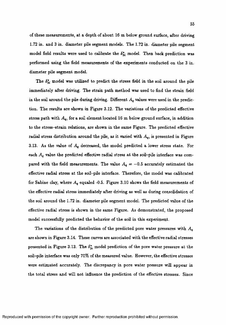
55
of these measurements, at a depth of about 16 m below ground surface, after driving
1.72 in. and 3 in. diameter pile segment models. The 1.72 in. diameter pile segment
model field results were used to calibrate the model. Then back prediction was
performed using the field measurements of the experiments conducted on the 3 in.
diameter pile segment model.
The &2 i model was utilized to predict the stress field in the soil around the pile
immediately after driving. The strain path method was used to find the strain field
in the soil around the pile during driving. Different A q values were used in the predic
tion. The results are shown in Figure 3.12. The variations of the predicted effective
stress path with A q, for a soil element located 16 m below ground surface, in addition
to the stress-strain relations, are shown in the same Figure. The predicted effective
radial stress distribution around the pile, as it varied with Aq, is presented in Figure
3.13. As the value of Aq decreased, the model predicted a lower stress state. For
each Aq value the predicted effective radial stress at the soil-pile interface was com
pared with the field measurements. The value A q = —0.5 accurately estimated the
effective radial stress at the soil-pile interface. Therefore, the model was calibrated
for Sabine clay, where Aq equaled -0.5. Figure 3.10 shows the field measurements of
the effective radial stress immediately after driving as well as during consolidation of
the soil around the 1.72 in. diameter pile segment model. The predicted value of the
effective radial stress is shown in the same Figure. As demonstrated, the proposed
model successfully predicted the behavior of the soil in this experiment.
The variations of the distribution of the predicted pore water pressures with A q
are shown in Figure 3.14. These curves are associated with the effective radial stresses
presented in Figure 3.13. The model prediction of the pore water pressure at the
soil-pile interface was only 70% of the measured value. However, the effective stresses
were estimated accurately. The discrepancy in pore water pressure will appear in
the total stress and will not influence the prediction of the effective stresses. Since
Reproduced with permission of the copyright owner. Further reproduction prohibited without permission.

56
20
K„ condition
CDQ.
QCM“D
A = 0.0
A = -0.3
A = -0.5
Aq= -0.7
A = -0.9
0 100 200 300
J-, , kPa
(a)
CDQ.
QCM
20
10
0.0 0.1 0.2
* 2 D
0.3 0.4
(b)
Figure 3.12: (a) Variation of effective stress path with Aq during pile driving as predicted by the model, using strain path method; (b) The corresponding predicted stress-strain relationships.
Reproduced with permission of the copyright owner. Further reproduction prohibited without permission.

Reproduced
with perm
ission of the
copyright ow
ner. Further
reproduction prohibited
without
permission.
100 "i------------1-------- 1— i— i— i i i [
75roQ.</>'inSin.5 50TJS©>'■sit=UJ 25 A—A a
Q 0 - 0 ----0 O "0
□ □ B -------- □ □ □ □ H o
f r o O O 8 0
- v 00
- v a3
- V -0 5
s— v a7- 0
J i i i i i i
10 100
Normalized distance from pile wall (r/r0)
Figure 3.13: Predicted distribution o f effective radial stress for different Aq values immediately after pile driving, using the 5*2j model.

Reproduced
with perm
ission of the
copyright ow
ner. Further
reproduction prohibited
without
permission.
(OCLX.e3(AWd)
£to£2on
250
225
200
175
15010 100
Normalized distance from pile wall (r/r„)
Figure 3.14: Predicted distribution o f pore water pressure for different Aq values immediately after pile driving, using the 8*2j model.
00

59
soil behavior depends on effective stresses, the model was considered satisfactory to
complete the proposed numerical study.
The model predictions of Sabine clay behavior were verified by simulating other
field experiments. Back prediction of the measured effective radial stress, at the
soil-pile interface around the 3 in. diameter pile segment model installed in Sabine
clay, is presented in Figure 3.11. The numerical results compare well with field
measurements, as shown in Figure 3.11. This demonstrates the capability of the
model to predict the behavior of the soil at Sabine Pass, Texas.
Reproduced with permission of the copyright owner. Further reproduction prohibited without permission.

CHAPTER 4 SIMULATION OF PILE INSTALLATION
4.1 Introduction
The installation process severely remolds and disturbs the soil around the pile and
generates changes in the pore water pressures. These effects greatly influence pile
performance. Simulation of the pile driving process provides the initial conditions
for subsequent consolidation and loading. Therefore, it is necessary to adopt a reli
able method to simulate pile driving and then to obtain the deformation field in the
surrounding soil. The accurate estimation of these deformations results in appro
priate predictions of the stresses and pore water pressures. There are three major
methods that can be used to simulate pile driving: the cavity expansion method, the
strain path method, and the large-strain finite element method. Among the different
methods available to simulate pile driving, the strain path method, as proposed by
Baligh (1975, 1985), was successfully used to solve deep penetration problems such
as: simple pile (Baligh, 1975; 1984; 1985; 1986); cone penetrometers (Levadoux and
Baligh, 1980); open-ended piles (Chin and Baligh, 1983); soil samplers (Baligh et al.
1987); and closed-ended pile segment models (Wathugala, 1990). This method was
used to simulate pile driving in the current study.
This chapter presents the aspects of simulation of pile driving using the strain
path method. Regarding the present study, the strain field around the closed-ended
pile (simple pile) was obtained using formulas, while a numerical scheme was used
to develop a computer code for the open-ended pile.
60
Reproduced with permission of the copyright owner. Further reproduction prohibited without permission.

61
4.2 M ethods o f Pile Driving Simulation
The behavior of piles driven into saturated clay is governed by the effects of driv
ing, subsequent consolidation, and loading on the clay-water system. In order to
understand the behavior of the pile, these effects may be studied using the most
reliable and practical methods. Theoretical and numerical studies, using different
methods, have been conducted to simulate these effects. Cavity expansion methods,
or CEMs, are the most popular ones used to simulate pile driving. The simplicity
of CEMs (due to the one-dimensional nature of the cavity expansion) has enabled
investigators to obtain analytical and numerical solutions (Butterfield and Banerjee,
1970; Carter et al., 1979).
However, the CEM cannot capture the two dimensional nature of the pile driving
problem. Because the actual deformations (due to driving) near the top and the tip
of the pile do not occur radially, as the cylindrical CEM postulates. In addition, the
strain path assumed in the CEM is not realistic and can lead to errors because soils,
in general, are strain path dependent. While cavity expansion methods are helpful
in developing a qualitative understanding of the problem, they are not a complete
solution.
Exact simulation of pile driving is difficult. The usual procedure would be to
start from an initial state of stress and pore water pressures and then to simulate the
process of driving as the pile is pushed into the ground. Desai (1978) proposed using
a large-strain finite element formulation for this purpose. Kiousis et al. (1988) used
a similar approach to solve the cone penetration problem, utilizing the large—strain
finite element method and the Cap model (DiMaggio and Sandler, 1971). The Cyber
205 supercomputer took 20 cpu hours for 20 mm advancement of the cone penetrom
eter. Consequently, with available computing power, it would be very expensive to
exactly simulate pile driving, which needs severed meters of advancement.
Reproduced with permission of the copyright owner. Further reproduction prohibited without permission.

62
Evidence from Experiments (Rourk, 1961; Vesic, 1963; Robinsky and Morrison,
1964; Szechy, 1968; Randolph, et al., 1979) confirmed that the deformations caused
by the penetration of a rigid indenter axe similar in different soils, even though
the penetration resistance can be drastically different. This implies that the pile
installation is a strain controlled problem and that the deformations associated with
it are not very sensitive to soil behavior (Levadoux and Baligh, 1980). Based on
these observations, Baligh and co-workers (1975, 1984, 1985, and 1986) developed
the Strain Path Method (SPM), to obtain solutions for different deep penetration
problems including pile driving. Their method is based on getting a kinematically
admissible deformation field for the particular problem, by using analytical solutions
of uniform inviscid flow around sinks and sources. By distributing different sources
of variable strength in the uniform flow, deformation fields were obtained around: (a)
the simple pile (Baligh 1975, 1984, 1985, and 1986), (b) cone penetrometers (Baligh
and Levadoux, 1980), (c) open ended piles (Chin and Baligh, 1983), and (d) soil
samplers (Baligh et al., 1987). The strain path at each point can be calculated from
the deformation field. Then the effective stress path corresponding to the strain
path can be determined from the constitutive equations. Total stresses and pore
water pressures can be obtained by solving the equilibrium equations. It should be
noted here that the final stresses and pore pressures will be exact if and only if the
estimated deformation fields are identical to those experienced in the actual problem.
Tumay et al. (1985) and Acar and Tumay (1986) proposed a strain path method
based on a semi-analytical technique to obtain deformation patterns around cone
penetrometers (this method uses the conformal mapping rather thcin sources and
sinks, as in the strain path method).
Reproduced with permission of the copyright owner. Further reproduction prohibited without permission.

63
4.3 Strain Path M ethod
The strain path method is an approximate analytical technique that utilizes the so
lution for steady irrotational flow of an inviscid incompressible fluid to solve deep
penetration problems. The basic idea of this approach is to obtain a kinematically
admissible deformation field for the particular problem by superimposing flow due
to different sources and sinks into a uniform steady flow coming from infinity. Com
bining a uniform steady flow with a flow resulting from a simple source yields the
solution for the simple pile, while replacing the simple source with a ring source
produces the solution for the open-ended pile.
4.3.1 Limitations
The strain path method simulates deep, steady, quasi-static, two-dimensional, undrained
penetration of axisymmetric piles in saturated (incompressible) homogeneous isotropic
clay initially subjected to an isotropic state of stress. These conditions cannot be met
in the case of piles driven into A"0-consolidated soils. Moreover, the method neglects
the surface roughness of the pile wall. This implies that the predicted deformation
field will only be approximate and therefore stresses and pore pressures estimated by
this method will also be approximate. However, experimental observations (Rourk,
1961; and Randolph et al., 1979) have suggested that the deformation field predicted
through these approximations may be considered the best available solution for deep
penetration problems.
4.3.2 C losed-Ended P iles
The simple pile approach (Baligh, 1975) was proposed to investigate the installation
effects of the simple solid (closed-ended) pile on the surrounding soil. The solution is
based on the principles and assumptions of the strain path method. Superimposing
Reproduced with permission of the copyright owner. Further reproduction prohibited without permission.

64
the flow resulting from a simple source (a point of outward radial flow) and a uniform
steady flow, provides the formulation for the simple pile problem.
Considering a cylindrical coordinate system with radial axis r and vertical axis z,
the stream function for a uniform steady flow of velocity U is given by (Thompson,
1976):
rp = Ur2 (4.1)
the stream function corresponding to a simple source emitting a fluid of volume equal
to 47rm per unit time (where m is the strength of the source) is given by (Thompson,
1976):
ip = m cos (p = m ------------j- (4-2)(r2 + z2)?
superposition of the stream functions, in Equations 4.1 and 4.2, yields:
ip = ~ ~ U t 2 + mcos <p (4-3)
the dividing stream line equation can be written as:
(^ ) = ^ [1 + cos^ (4-4)
this equation gives the geometry of a blunt-nosed cylindrical body whose diameter
at z = oo or (<p = 0) is 2R which is known as the simple pile. The geometry of the
simple pile is shown in Figure 4.1.
The path of a soil particle initially located at a radial distance r„ from the center
line of the pile can be obtained from (Baligh, 1985a):
<«>where R is the radius of the pile shaft.
R eproduced with perm ission of the copyright owner. Further reproduction prohibited without perm ission.

65
Stream line
► r
Stream line not drawn to scale
Figure 4.1: Geometry o f the simple pile.
R eproduced with perm ission of the copyright owner. Further reproduction prohibited without perm ission.

66
The semi-analytical solution for strains obtained by Baligh (1985) is only ap
proximate, because it is based on the simplifying assumption that the stream lines
are vertical. This implies that this solution is not exact and is only valid in the far
field, where stream lines are nearly parallel to the pile axis. Teh and Houlsby (1987)
considered the actual curved profile of the stream line and derived the following exact
analytical expressions for strains around the simple pile:
(4.6)
= -Fl(rf) - j(l - 3B*)fi(*) (4.7)
(4.8)
- (2B y /B 2 - l) tan -1 cot
sin(2$)
(4.9)
where err, ezz, egg, and eTZ are the radial, vertical, tangential, and shear strain
components, respectively, and
= 3(1 + cos (<£))[ ©
2 3 cos (<f>)(4.10)
F2(4) = b fl + i (^) (1 + cos(0)) (4.11)
B = 2(s ) ! + i <412>The modified strain field Equations 4.6, 4.7, 4.8, and 4.9 (Teh and Houlsby, 1987)
were used in this study to estimate the strain field in the soil around the closed-ended
R eproduced with perm ission of the copyright owner. Further reproduction prohibited without perm ission.

67
(or simple) pile. Figure 4.2 shows the predicted strain field around the simple pile for
soil elements located initially at radial distance ra = R and ra = 2R, respectively. In
this figure, the amount of strain is almost negligible when the soil element is located
at a vertical distance more than 5R in front of the tip of the pile. Then, as the soil
element approaches the tip of the pile, higher strains are induced by driving. The
magnitude of the radial and tangential strains increases as the soil element passes
the tip and then remains constant at a vertical distance of about 5R behind the tip
of the pile. The vertical strain vanishes at almost the same vertical distance, while
shear strain decreases to a very low value then remains constant. The variation with
radial distance of strains in the soil around the pile at the end of driving is presented
in Figure 4.3. High strains are developed at the pile-soil interface. The amount of
strain decreases with the increase in the radial distance away from the pile until it
becomes negligible in the far field.
4.3.3 O p en -E n d ed Piles
The mechanism of open-ended (cookie cutter or totally unplugged) pile driving was
investigated, via the strain path method, by Chin and Baligh (1983). Simulation
of an open-ended pile installation was performed using the method of sources and
sinks, by combining the flow of a ring source with a uniform steady flow. In the strain
path method, the pile is considered an “ideal” open-ended pile if it is simulated by
superimposing one ring source on a uniform steady flow. Different pile geometries can
be obtained by considering different numbers and arrangements of the ring sources in
the uniform flow. Using the cylindrical coordinate system, the formulation presented
herein describes the penetration of axisymmetric “ideal” open-ended pile.
R eproduced with perm ission of the copyright owner. Further reproduction prohibited without perm ission.

68
5.0
tr
8 2 5 -ceg]35T 3
ro0.0 -
®>TJ®NtO j c _§ 2 5 Oz
-5.0- 0.2-0.4 0.20.0 0.4
Strain, %(a)
5.0
CE15g 2.5ctoCOT315
o.o -0)>TJ0)N1 -2.5 -
r J R = 2.0
oz
-5.0- 0.2-0.4 0.20.0 0.4
Strain, %
(b)
Figure 4.2: Strain field around simple pile for (a) Soil element located initially at r0=R, (b) Soil element located initially at r0=2R.
R eproduced with perm ission of the copyright owner. Further reproduction prohibited without perm ission.

69
CM
in
©ocra"wT>raTJ5
T 30)NraEo
04
o£I!N.£H.c3S00c
■3o
' i
<D.2•3UHE
&e*3oco3
r2*CC/3scnrOw300
in ino
oo
tno'
% ‘UIBJJS
Reproduced with permission of the copyright owner. Further reproduction prohibited without permission.

70
4.3.3.1 R ing Source
The ring source is a distribution of constant strength sources along a circle. The
velocity components of a ring source of radius R placed in the plane z — 0 and
emitting an incompressible fluid at a rate of volume V per unit time in an infinite
medium are (Kuchemann and Weber, 1953):
V
4 * 2 v j z 2 + (r + R ) 2
v° = V 2 z-E(k)
(4.13)
(4.14)‘ 4* 2 yjz2 + (r + R ) 2 [z2 + (r - fl)2]
where v° is the radial velocity, v° is the vertical velocity (in the cylindrical coordinate
system), and k is the particle position parameter which is given by
4 tRh z 2 + (r + R ) 2 (4‘15)
the functions K {k ) and E(k) are complete elliptical integrals of the first and second
kind, respectively, and are given by:
K M = nJ o V r^ fc s in ^ a
da (4.16)
E(k) = f 3 y jl — k sin2 a da (417)Jo
the complete elliptical integrals can be evaluated through the following polynomial
approximation (Abramowitz and Stegun, 1964):
K{m) = + axm x + a2 m \ + a3 m \ + (4-18)
(=r)+ [&o + bxm x + b3 m \ + b3m l + In f — 1
+ e(m) | e(m) |< 2 x 10 - 8
Reproduced with permission of the copyright owner. Further reproduction prohibited without permission.

71
where m i = 1 — m, and 0 < m < 1; and
a0 = 1.38629436112
a\ = 0.09666344259
a2 = 0.03590092383
a3 = 0.03742563713
a4 = 0.01451196212
and
b0 = 0.5
&i = 0.12498593597
b2 = 0.06880248576
b3 = 0.03328355346
64 = 0.00441787012
E(m ) = £l + a-[TTi\ + a2 m \ + 03771 + a4m ij
+
+ e(m)
where
= 0.44325141463
a2 = 0.06260601220
a3 = 0.04757383546
a4 = 0.01736506451
+ b2 m \ + b3 vn\ + 64m^j In
| e(m) |< 2 x 10'
fcx = 0.24998368310
b2 = 0.09200180037
63 = 0.04069697526
64 = 0.00526449639
(4.19)
4.3.3.2 Superposing a Uniform Steady Flow on the Source—Ring Flow
The solution for the open-ended pile is achieved by superposing a uniform steady
flow of velocity U on the flow of a ring source. As a result, an annular body of infinite
length is obtained, which is the geometry of the open-ended pile. Figure 4.4 shows a
diagram for the geometry of the open-ended pile. In a cylindrical coordinate system,
the velocity components of a particle moving in the combined flow are
Reproduced with permission of the copyright owner. Further reproduction prohibited without permission.

B = 2R
soilInnerOutersoil
Particle path
Particle path not drawn to scale
Figure 4.4: Geomerty of the open-ended pile.
Reproduced with permission of the copyright owner. Further reproduction prohibited without permission.

73
vr = v° and vz = v° + U (4.20)
where vr and vz are the radial and vertical velocity components, respectively, and v°
and v° are the radial and vertical velocity components of the ring source as given by
Equations 4.13 and 4.14, respectively.
The relation between the aspect ratio of an open-ended pile, B / t (where B is
the diameter and t is the wall thickness of the open-ended pile), and the discharged
volume of the source fluid, V, can be obtained from the continuity as follows:
V = t U ( R 2 - R]) (4.21)
where R and Ri axe the outer and inner radii of the open-ended pile far behind the
tip, respectively. Defining the wall thickness t as t = R — f?,-, Equation 4.21 can be
approximated as :
V ~ 2trRtU, 4 < 1 (4.22)K
or
B B2irU— ~ ——— where B = 2R (4-23)
this approximation is acceptable since most of the open-ended piles in the engineering
practice have an aspect ratio of 17 < B / t < 44 (Azzouz and Baligh, 1984).
4.3.3.3 S tra in F ield
The coordinates of a material point Mi a t time t with initial coordinates r° and z°
far enough in front of the tip of the pile are given by
ri = r° + [ Vr(ri>zi)dT (4.24)Jo
Reproduced with permission of the copyright owner. Further reproduction prohibited without permission.

74
z\ = z\ + f v z ( t J , zT)dr (4.25)Jo
where vr and vz axe the radial and axial velocity components in the cylindrical
coordinate system, respectively. These components are given by Equation 4.20. The
tangential velocity vg vanishes because of axial symmetry.
The rate of deformation tensor, Dij, is given as follows
where ut- are the velocity components. The following components of the rate of
deformation tensor, D ^, during axisymmetric penetration in an infinite medium are
derived from Equation 4.26.
n - dVr n - dVz n — Vf n _ 1 ( dVr a o7^r r ~ dr ' z z ~ d z ' _ r ’ r z ~ 2 [ d z + d r ) ( }
where vr and vz are the radial and vertical velocity components, respectively.
The natural strain increment, detJ-, is introduced to determine the strain field in
the soil around the pile during driving
£ij = J deij = J Dijdt (4.28)
the integration is conducted by following a particle on its path along the stream
line. During undrained penetration, the resulting strain components must satisfy
zero volume change condition, which means:
£rr + + £se — 0 (4-29)
The estimation of deformations, strain increments, and strains in the soil during
open-ended pile penetration is performed numerically, due to the complexity of the
Reproduced with permission of the copyright owner. Further reproduction prohibited without permission.

75
ring source formulation. A numerical procedure proposed by Levadoux and Baligh
(1980) for investigating the deformations and strains around the cone penetrometer
was adopted by Chin and Baligh (1983) for the open-ended piles. This method
was used, with modifications on the integration method, in this study to develop
a computer code to simulate the driving of open-ended piles. The following is a
general description of the main steps of this method:
1. The path of a soil particle during driving is obtained by numerical integration
of Equations 4.24 and 4.25. The radial and axial velocity components are
given by Equation 4.20. Small time increments are used with the mid-point
integration method.
2. During the particle motion along its path, at each time increment the com
ponents of the rate of the deformation tensor are calculated from Equation
4.27.
3. Natural strain increments are obtained by the numerical integration of Equa
tion 4.28 at each time increment. Strain components at time t are obtained by
adding the strain increments.
The strain field in the soil during the driving of open-ended piles was obtained
using the described numerical procedure. The effect of the penetration velocity on
the predicted strain field was investigated. Simulation of pile driving was performed
with different penetration velocities. Results indicated that the penetration velocity,
U, did not affect the predicted strain field, even though the rate of deformation of the
soil around the pile was influenced. Figure 4.5 shows the strain field determined by
the strain path method resulting from the driving of open-ended piles with different
penetration velocities.
The predicted strain field for a soil element located, at the end of driving, at
distance 77 = 1.5fZ outside the wall, is shown in Figure 4.6a. The strain field for
Reproduced with permission of the copyright owner. Further reproduction prohibited without permission.
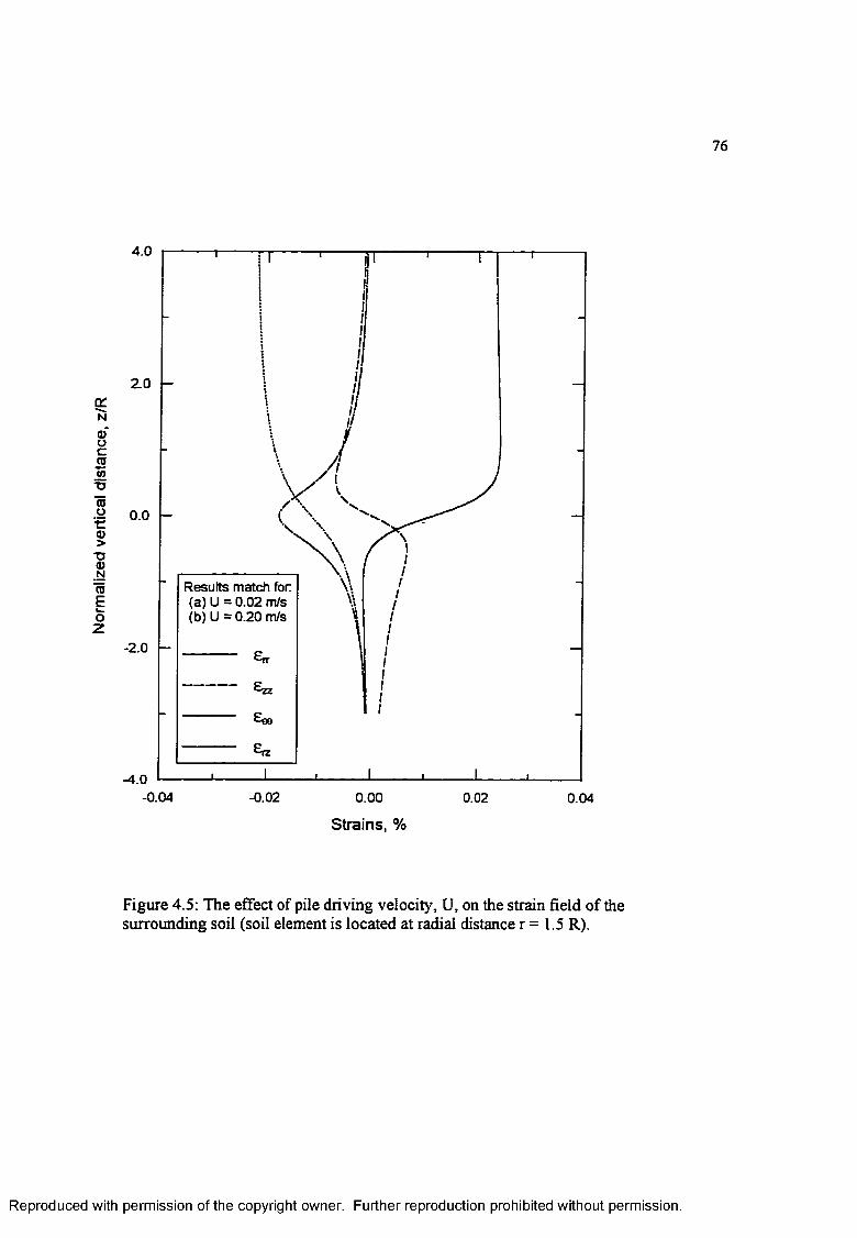
Nor
mal
ized
ve
rtic
al d
ista
nce,
z/R
76
4 .0
2.0
0.0
Results match for(a) U = 0.02 m/s(b) U = 0.20 m/s
- 2.0
-4.0-0.04 - 0.02 0.00 0.02 0.04
Strains, %
Figure 4.5: The effect of pile driving velocity, U, on the strain field of the surrounding soil (soil element is located at radial distance r = 1.5 R).
R eproduced with perm ission of the copyright owner. Further reproduction prohibited without perm ission.

Reproduced
with perm
ission of the
copyright ow
ner. Further
reproduction prohibited
without
permission.
a:■aofocain‘o8■e<1)>~o0)NID§oz
4
2
0
■2
-0.04 - 0.02 0.00 0.02 0.04
O'
ofoca</)8€a>>■oa>Nra§o
4
2
0
■2
•rz
-0.04 - 0.02 0.00 0.02 0.04
Strain
(a) r,=1.5R
Strain
(b) r,=15t
Figure 4.6: Strain field predicted by SPM due to an open-ended pile driving; (a) Soil element outside the pile located finally at radial distance rf=1.5R; (b) Soil element inside the pile located finally at radial distance r,^15t.
-j

78
this element is similar to the strain field obtained around the simple pile. Figure
4.6b presents the strain field for a soil element located inside the wall at a distance
77 = 15f from the center of the open-ended pile at the end of pile driving.
The strain paths for two soil elements located, at the end of driving, in the
immediate vicinity of the pile wall are presented in Figure 4.7. The strain paths are
presented in the deviatoric f?t—space where Ei, Et and E3 are defined as:
Ei = ezz
Et = ^ (e V r - )
E3 = ~^2 ,£rz (4.30)
the strain path moved along E\ for the triaxial test, along Et for the pressuremeter
test and along E 3 for the direct simple shear test. As shown in Figure 4.7, the soil
elements were located at 77 = r — 1.2£ inside and 77 = r + 1 outside the wall of the
pile. These elements were subjected to severe shearing and strain reversals. The
outside element, for example, experienced about 60% strain along the Ez-zxis (i.e.
the direct simple shear mode).
4.4 Numerical Simulation o f Pile Driving
In this study, the general procedure described by Wathugala (1990) is modified and
used to obtain the distribution of effective stresses, total stresses, pore water pres
sures, and hardening parameters in the soil, as follows:
1. The strain path method provides the strain path for a soil particle during pile
driving. Determination of the strain path due to pile driving is performed at
all Gauss points in the finite element mesh.
Reproduced with permission of the copyright owner. Further reproduction prohibited without permission.

CJII
liT
- 0.1
o.o
0.1
0.2
0.4
= r-1.2t
= r+t0.3 -
s t / /
-0.2 -0.1 0.0
E2 = (Err* %)A/3
0.1
CO-ycu_CMII
COHI
0.6
0.4
0.2
0.0
rf =r-1.2t
rf = r+t
- 0.2- 0.1 0.0- 0.2 0.1
B,= (V e«t)/V3
Figure 4.7: Strain paths, in the deviatoric space, o f soil elements located at the immediate vicinity outside and inside the wall during open-ended pile driving; (a) E, vs E2, (b) E3 vs E2.
Reproduced with permission of the copyright owner. Further reproduction prohibited without permission.

80
2. The corresponding effective stress path for each point is determined by inte
grating the constitutive equations along the given strain path. The proposed
H iSS-^i model through the ‘strain to stress’ algorithm is utilized to fulfill this
purpose.
3. The pore water pressures, effective stresses, and hardening parameters calcu
lated in step 2 are supplied to the finite element program ABAQUS/Standard
as input data. Distributions of pore water pressures, total stresses, effective
stresses, and hardening parameters that simultaneously satisfy equilibrium
equations, strain compatibility, and constitutive equations are computed by
ABAQUS/Standard. These distributions are calculated under undrained con
ditions, because pile driving is assumed to occur under these conditions. The
results at the end of the pile driving simulation are used as initial conditions
for the subsequent consolidation stage.
This procedure was applied to simulate the driving process for closed-ended and
open-ended piles. The effective stress path during driving for a soil element at the
pile-soil interface is presented in Figure 4.8. Point A in the Figure represents the
AT0-condition before pile driving. As the pile penetrated the soil, the state of stress
decreased until point B was reached at the end of driving. The distribution of effective
stresses at the end of driving is depicted in Figure 4.9. As shown in the Figure, a
low state of stress was predicted for the soil at the pile-soil interface as a result of
severe shearing. ff0-conditions were estimated for the soil in the far field, where
the strains developed due to driving were negligible. The corresponding predicted
pore water pressure distribution is shown in Figure 4.10. High pore water pressure
was predicted at the pile-soil interface, while hydrostatic pore water pressure was
estimated in the far held.
Reproduced with permission of the copyright owner. Further reproduction prohibited without permission.

Reproduced
with perm
ission of the
copyright ow
ner. Further
reproduction prohibited
without
permission.
Stress path during pile driving
Yield surface
Phase change line
20raCL
0 50 150100 200 250 300
J, , kPa
Figure 4.8: The predicted effective stress path for a soil element at the pile-soil interface during pile driving.
00

Reproduced
with perm
ission of the
copyright ow
ner. Further
reproduction prohibited
without
permission.
150
125(UCL-sc 100</)'w0)5 75u>0)I 50
LLI or
'oo
■e—o o o ooooocojooaMiiixx)— e—o o o o o o o o o
1 10 100Normalized distance from pile wall (r/r„)
Figure 4.9: Predicted distribution of effective stresses immediately after pile driving.

Reproduced
with perm
ission of the
copyright ow
ner. Further
reproduction prohibited
without
permission.
(OCL
8>3atatfl>
0)ro£a>oQ.
250
225
200
175
1 _ J L j . i X J 1 I I I J .150 x x j i i i
10 100
Normalized distance from pile wall (r/r0)
Figure 4.10: Predicted distribution of pore water pressure immediately after pile driving.
OOu>

CHAPTER 5VERIFICATION: PILE DRIVING,
SUBSEQUENT CONSOLIDATION AND PILELOAD TESTS
5.1 Introduction
In this study, a general method for predicting pile setup is proposed and verified. The
solution is based on a consistent formulation during the different life stages of a pile.
Utilized to achieve the objectives of this research are: the HiSS modeling approach
(Desai et al., 1986; Wathugala, 1990; Wathugala and Desai, 1993), the strain path
method (Baligh, 1975, 1984 and 1985; Levadoux and Baligh, 1980; Chin and Baligh,
1983), and the coupled theory of the nonlinear porous media formulated in the finite
element program ABAQUS/Standard (Hibbitt, Karlsson & Sorensen, INC., 1995).
The soil behavior was characterized by the proposed HiSS-^,- model (discussed
in detail in Chapter 3). The strain path method was used to simulate the pile driving
process. The conditions at the end of driving were used in the finite element program
ABAQUS/Standard to start the consolidation phase. This program uses the cou
pled theory of the nonlinear porous media to solve different geotechnical engineering
problems including consolidation. During the consolidation phase, different pile load
tests were simulated.
It is necessary to verify and evaluate the proposed method based on existing field
experiments. The verification scheme is important in order to check the validity of
the numerical solution and to asses the possibility of using the method in future
applications.
This chapter presents the verification of the proposed method. Field experiments
performed on a 1.72 in. (4.37 cm) diameter pile segment model installed at Sabine
84
Reproduced with permission of the copyright owner. Further reproduction prohibited without permission.

85
Pass, Texas, were used for this purpose. The verification included the pile driving
process, subsequent consolidation, pile load tests conducted during consolidation,
and the final cyclic pile load test.
5.2 Field Tests at Sabine Site
The field experiments conducted by the Earth Technology Corp. (1986) on Sabine
clay were employed to verify and evaluate the current theoretical and numerical
study. These experiments were performed at a depth of 50 ft (15.24 m), using two
instrumented pile segment models of 1.72 in. (4.37 cm) and 3 (7.62 cm) in. in
diameter. Changeable cutting shoes with different wall thicknesses were attached
to these models in order to conduct measurements on open-ended piles. Table 5.1
presents the dimensions of these pile segment models. These models were equipped to
measure simultaneously the total radial pressure, pore pressure, shear transfer, and
relative pile-soil displacement, during driving, consolidation, and static and cyclic
load tests.
The testing program was initiated: (a) to examine the effects of the diameter/wall
thickness ratio, D /w t , on the rate of consolidation and setup; (b) to study the effects
of the diameter, D, on the rate of consolidation and setup; and (c) to investigate
the role of the effective radial pressure and pore water pressure with regard to the
axial shear transfer capacity. This well-documented study provided high quality
experimental data in the area of axial pile-soil interaction and therefore was used
for the verification and evaluation scheme.
5.2.1 T est Procedures
The test procedure sequence for each experiment is described in Figure 5.1. One
of the main objectives of these experiments was to study the evolution of the static
Reproduced with permission of the copyright owner. Further reproduction prohibited without permission.

86
Table 5.1: Dimensions of the pile segment models used in the field experiments.
Diameter (D), in. (cm) Wall thickness (wt), in. (cm) D/wt
1.72 (4.37) - 2 (closed-ended)
3.0 (7.62) - 2 (closed-ended)
3.0 (7.62) 0.125 (0.318) 24 (open-ended)
3.0 (7.62) 0.065 (0.165) 46 (open-ended)
Reproduced with permission of the copyright owner. Further reproduction prohibited without permission.

87
Setting up the loading system at the top of the borehole
Drilling and casing the bore holes up to the test depth
Lowering the pile segment model into the borehole
Attachment of the data acquisition system to the pile segment model
Performing the final two-way cyclic load tests at the end of consolidation
Conducting static tension and compression tests during consolidation
nstallation of the models by pushing the X-probe or driving the 3 in. diameter pile segment model
Continuously measuring the pore pressure, the shear transfer, the total radial pressure, and the relative soil-pile displacement
Figure 5.1: The test procedure sequence for the field experiments.
Reproduced with permission of the copyright owner. Further reproduction prohibited without permission.

88
shear transfer capacity during consolidation. Therefore, it was decided to perform
load tests at degrees of consolidation of 20, 40, 60, 80 and 90 percent and more.
However, the load tests were conducted at degrees of consolidation close to the
predetermined ones.
5.2.2 P ile Segm ent M odels
Two pile segment models with changeable cutting shoes were used in Sabine field
experiments: the 1.72 in. diameter pile segment model (also known as the X-probe)
and the 3 in. diameter pile segment model. The 1.72 in. diameter pile segment
model is shown in Figure 5.2. This model has a length of 56.5 in. (1.44 m). It
is equipped with a total pressure transducer, a pore pressure transducer, a shear-
sensing element (friction sleeve), and a displacement transducer. Figure 5.3 shows
the 3 in. diameter pile segment model. This probe is instrumented with: load cells
(for friction measurements), total and pore pressure transducers, and DC-LVDT (for
measurements of the relative pile-soil displacement). Detailed information about
these models and the test setup was presented in the studies conducted by Earth
Technology Corp. (1986) and Wathugala (1990).
5.2.3 R esults of Field Experim ents
Presented herein are the results of the field experiments conducted on the 1.72 in.
diameter pile segment model. The measurements taken during the pile driving are
not available. The measured total radial and pore water pressures during the con
solidation phase are shown in Figure 5.4. The corresponding calculated effective
radial stress variation is also presented in the same figure. The breaks in the plots
correspond to the time at which pile load tests were performed. It can be noted that
the static load tests have only minor effects on the consolidation phase (Earth Tech
nology Corp., 1986). Pile load tests were performed during consolidation in order to
Reproduced with permission of the copyright owner. Further reproduction prohibited without permission.

89
INSTRUMENT CABLE
STANDARD CONE ROD CONNECTION
LOAD CELL
TOTAL PRESSURE CELL
PORE PRESSURE CELL
DISPLACEMENT TRANSDUCER
SOIL ANCHOR
Figure 5.2: The 1.72 in. diameter pile segment model (after Earth Technology Corp., 1986).
Reproduced with permission of the copyright owner. Further reproduction prohibited without permission.

90
O R IL L RO D ADA PTER
Ca b l e j u n c t i o n
SPACER
LOAO CELL
SPACER
HOU SING FO R TO TA L A N D PORE PRESSU R E
TRAN SD U CERS
SPACER
LOAO C ELL
O O L V D T HOUSING
i n t e r c h a n g e a b l e CUTTIN G SHOE
• SEE O E T A 1L A
> SEE / D E T A IL b
; SEE / D E T A IL A
ITlUUf; tAZtZD E T A IL A
Ulf VI MtXU |LOAO CELL FOR
FRICTION MEASUREMENT
' SEE D ETA IL C
D E T A IL B
T O T A L P R E S S U R E L O A D C E L L A N D P O R E P R E S S U R E
T R A N S D U C E R H O U S IN G
t 0 E T A 1 L C
I D C -L V D T F O RI M E A S U R E M E N T O F
/ R E L A T IV E D ISPL A C E M E N Te r r t iM C s n o c
Figure 5.3: The 3 in. diameter pile segment model (after Earth Technology Corp., 1986).
Reproduced with permission of the copyright owner. Further reproduction prohibited without permission.

Effe
ctiv
e ra
dial
pre
ssur
e, k
Pa
Radi
a to
tal
and
pore
pr
essu
re,
kPa
91
400
300
200 -
Total radial pressure
Pore water pressure
10010 100 1000 100001
Time after driving, min
(a) Total radial and pore water pressures.
200
100 -
10 1000 100001 100
Time after driving, min
(b) Effective radial pressure.
Figure 5.4: Variations of the measured pressures during soil consolidation around the 1.72 in. diameter pile segment model (after Earth Technology Corp., 1986).
Reproduced with permission of the copyright owner. Further reproduction prohibited without permission.

92
investigate the increase of bearing capacity with time (the pile setup). The results
of the measured shear transfer-displacement response for different tension pile load
tests are shown in Figure 5.5. Other results will be presented and compared with
the numerical solutions later.
5.3 T he Finite Element Program A B A Q U S/Standard
The general purpose finite element program ABAQUS/Standard (called ABAQUS in
this report) was used in the current study to perform the numerical simulation of the
consolidation phase and the pile load tests. The results of the numerical simulation
were processed through the post processing program ABAQUS/Post.
5.3.1 A nalysis o f Porous M edia
The analysis of porous media is treated in ABAQUS by the conventional approach.
The porous medium is considered a multi-phase material and the effective stress
principle is used to describe its behavior. The theory of deformation of porous media
as presented in the ABAQUS Theory Manual (Hibbitt, Karlsson & Sorensen, INC.,
1995) is summarized below. ABAQUS notations and sign conventions are used here.
The effective stress, a, acting at a point in the saturated porous medium, is given
by:
<r = <r + x u j i (5.1)
where a is the total stress, uw is the wetting liquid pressure (pore pressure), and
X is a factor that depends on the saturation and surface tension of the liquid-solid
system. For saturated systems, x = 1-0. In ABAQUS, tensile stress components are
stored as positive, which explains the sign in Equation 5.1.
R eproduced with perm ission of the copyright owner. Further reproduction prohibited without perm ission.

Reproduced
with perm
ission of the
copyright ow
ner. Further
reproduction prohibited
without
permission.
S . 20uT(ACsI—ro<u■Cw
Degree of consolidation
U = 22%
U = 60%
U = 87%
U = 98%
0.0E+0 3.0E-4 6.0E-4 9.0E-4 1.2E-3 1.5E-3
Displacement, m
Figure 5.5: Results o f the field static tension tests conducted on the 1.72 in. diameter pile segment model (after Earth Technology Corp., 1986).
v Ou>

94
The constitutive response of the porous medium includes the simple bulk elasticity
relationships for the pore fluid and the solid grains. Moreover, the material skeleton
behavior is determined by the constitutive theory in which the effective stress, <f , is
defined as a function of the strain history, the temperature, and the state dependent
variables.
The behavior of the porous medium is governed by the equilibrium and the con
tinuity equations. For the solid phase of the material, the stress equilibrium is
expressed by the virtual work principle for the volume V in its current configuration
at time t as:
J ( a - xtt*I) : SedV = J t ,8vdS+ j f.8vdV + J snpiofT.SvdV (5-2) v s v v
where 5e = sym(d8v/dx) is the virtual rate of deformation, a is the Cauchy effective
stress, 6 v is a virtual velocity field, t are surface tractions per unit area, f are body
forces per unit volume (excluding fluid weight), pw is the fluid density, and g is
the gravity acceleration. The Lagrangian formulation is used to discretize the solid
phase equation with the displacements as the nodal variables. In order to model the
porous medium, the continuity equation is required for the fluid phase. The equation
is obtained by equating the rate of increase in fluid volume stored at a point with
the rate of volume of fluid flowing into the point within the time increment:
/T ( I I = ~ f ^ r 37m -v todS (5-3)\ v P°w J s P°m
where v„ is the average seepage velocity (fluid velocity relative to the solid phase),
n is the outward normal to the surface S, s is the degree of saturation, and n is
the porosity. This continuity equation is normalized by the reference density of the
fluid p°w. The backward Euler approximation is used for the time integration of the
R eproduced with perm ission of the copyright owner. Further reproduction prohibited without perm ission.

95
continuity equation. For further details, the reader is referred to Section 2.6 in the
ABAQUS Theory Manual (Hibbitt, Karlsson & Sorensen, INC., 1995).
5.3.2 Im plem entation o f th e HiSS—£|t- M odel in A B A Q U S
The proposed EiSS-S^ model was implemented in the finite element program ABAQUS,
which allows the use of user defined subroutines. The HiSS- model was first in
corporated in the ‘strain to stress’ algorithm developed by Wathugala (1990) for the
HiSS-£* series models. This algorithm uses the incremental theory of plasticity to
predict the stress increment corresponding to a given strain increment during vir
gin loading, unloading, and reloading. The hardening parameters are also updated
during the incremental calculations.
The user defined subroutine, UMAT, was then used to implement the ‘strain
to stress’ algorithm into ABAQUS. UMAT is developed in ABAQUS to incorporate
any user defined material behavior into the finite element. This subroutine exchanges
information between the ‘strain to stress’ algorithm and ABAQUS. The information
includes the element number, Gauss point number, step number, iteration number,
time, total strains, incremented strains, predicted stresses, and updated hardening
parameters.
The initial conditions needed to be given to the finite element program before
starting the analysis. This was achieved through the user defined subroutines SIGINI
and SDVINI. The user subroutine, SIGINI, defines the initial stress field. The initial
stresses are calculated at each Gauss point in the finite element mesh. The subroutine
SDVINI is called to define the initial solution dependent state variable fields only
in the beginning of the analyses. The variable fields include the strain trajectories,
plastic strains, initial hardening function, and the flag that defines the virgin loading,
unloading, and reloading.
R eproduced with perm ission of the copyright owner. Further reproduction prohibited without perm ission.

96
The numerical simulation was performed in this study through a single set of user
subroutines. First, the pile driving process was simulated. The effective stresses and
hardening parameters were determined during pile driving at all Gauss points in the
finite element mesh. This was achieved through the ‘strain to stress’ algorithm used
to integrate the constitutive equations. The integration was performed along the
strain path for the Gauss point during pile driving. The strain field was predicted by
the strain path method. At the end of driving, ABAQUS performed globed iterations
to calculate the equilibrated effective stress and pore water pressure distributions.
The effective stresses, pore water pressures, and hardening parameters calculated at
end of driving were supplied to ABAQUS as initial conditions for the consolidation
phase. During the consolidation, each pile load test was simulated at a time equal
to the actual time of conducting the field test. Figure 5.6 shows a diagram for the
numerical simulation procedure.
5.3.3 F in ite Elem ent Mesh
The element library in ABAQUS contains a wide range of elements which provide
the geometric modeling capability for various applications. Due to the symmetry
around the pile axis, the axisymmetric solid element CAX8RP was selected to model
the geometry of the problem. This element is one of a variety of elements provided for
modeling coupled pore fluid diffusion/stress analysis problems. The nodal variables
for this element are the displacements and the pore pressure. The element CAX8RP
uses second-order (quadratic) interpolation for the geometry and displacements. The
pore pressure is interpolated linearly from the comer nodes. Reduced integration
scheme is recommended by Wathugala (1990) to avoid unstable prediction of pore
water pressures in this type of problems. This element is generally described as an
8-node biquadratic displacement, bilinear pore pressure, with reduced integration
scheme. The element CAX8RP and its characteristics are shown in Figure 5.7.
R eproduced with perm ission of the copyright owner. Further reproduction prohibited without perm ission.

97
Open-ended pile i Call KOPENDRIV!
Closed-ended pile Call KSPILE
Run ABAQUS
Call pile driving subroutines KINSITU (main)
Initial conditions before pile driving Call SIGINI Call SDVINI
_ Initial conditions at | the end of pile driving
; ABAQUS-UMAT
Stresses, pore pressures, hardening parameter and state dependent variables at the end of pile
j driving (initial conditions for consolidation)
Pile load tests including the final cyclic load test
Consolidation stresses, pore pressures, hardening parameters
(initial conditions for pile load test)
Figure 5.6: Diagram for the use of UMAT in the finite element analysis.
R eproduced with perm ission of the copyright owner. Further reproduction prohibited without perm ission.

98
4 7 3
8
21 5
Uz▲
p • --------------------► U r
• Node
+ Gauss point
up Radial displacement
uz, Vertical displacement
p, Pore water pressure (at nodes 1, 2, 3, and 4)
Figure 5.7: ABAQUS axisymmetric solid element CAX8RP used in the finite element analysis.
R eproduced with perm ission of the copyright owner. Further reproduction prohibited without perm ission.

99
The finite element mesh used to simulate the consolidation and pile load tests for
the 1.72 in diameter pile segment model is shown in Figure 5.8. The mesh consists
of 578 elements and 1837 nodes. The analysis was started using a coarse finite
element mesh. This mesh led to numerical oscillations in pore water pressures. The
mesh was then refined until these numerical oscillations disappeared. The mesh was
generated so that small size elements were used around the pile. This was necessary
for accurately capturing the response in the surrounding soil where laxge deformations
were developed. Moreover, the fine mesh arrangement leads to numerical stability
and faster convergence.
The H iSS-^i model was proposed in this study to characterize the soil behavior
at the interface. As presented in Chapter 3, this model has the capability to predict
the stress state beyond the phase change line (critical state line). Such a stress
condition results from the high shear deformations at the soil-pile interface. On the
other hand, the HiSS-£j model predicts the state of failure at the phase change line.
Therefore, up to a certain degree of straining, both models predict almost similar
stress conditions before the phase change line. This is illustrated in Figure 5.9. The
strain field during pile driving for soil elements (A, B, C and D) located at different
radial distances from the pile surface was determined. Then the HiSS-j^ model was
used to predict the corresponding stress path for these elements, as shown in the
figure. The stress points at the end of driving passed the phase change line when soil
elements were located at radial distances 1.5R and 5R (elements C and D). On the
other hand, the stress point stopped before the phase change line for the element at
6.5R from the pile center line (element B). The far field element A remained under
AT0-condition both before and after driving.
The predictions of the HiSS-tf ,- and models were similar when the elements
were located at a radial distance of more than about 6.5R from the center line of
the pile. Therefore, it was expected that the interface model BSSS-fJ,- would be used
Reproduced with permission of the copyright owner. Further reproduction prohibited without permission.

fi> <5 T
< 5
< s
Element. 8-node ABAQUS-CAX8RP 578 elements 1837 nodes
Figure 5.8: The finite element mesh used to discretize the soil domain around the 1.72 in. diameter pile segment model.
Reproduced with permission of the copyright owner. Further reproduction prohibited without permission.

Pile Ground surface
(a) The location of the elements.
CDO.
□CM
30
Yield surface
Phase change line
Radial distance = 1.5R
Radial distance = 5R20
Radial distance = 6.5R
10
00 100 200 300
J1 , kPa
(b) The stress paths.
Figure 5.9: Variation with radial distance of predicted effective stress paths during pile driving for soil elements located 16 m below the ground surface.
Reproduced with permission of the copyright owner. Further reproduction prohibited without permission.

102
for the soil around the pile up to about 6.5R radial distance, and the HiSS-£g model
would be used for the soil beyond this distance. However, the difference between the
predictions of the HiSS-tfJ,- and Sq models is negligible before the phase change line
is reached. Therefore, the whole soil domain around the pile was modeled using the
interface HiSS- f t model.
5.4 P ile Driving
As described in Figure 5.1, the 1.72 in. diameter pile segment model was driven at
the bottom of the bore hole. The soil from the ground surface down to the bottom of
the bore hole was assumed to be at AT0—condition. The soil below the bottom of the
bore hole was affected by pile driving. The strain path method was used to estimate
the strain field in the soil around the pile during driving. The 1.72 in diameter pile
segment model is a closed-ended pile and therefore the pile driving was simulated
utilizing the simple pile approach (Baligh, 1984). Simulation of pile driving was
presented in detail in Section 4.3.
The soil element located at the soil-pile interface at a depth of about 16 m was
used for verifying and evaluating the numerical results. This depth corresponded to
the location of the radial and pore water pressure transducers in the field experiments.
The predicted effective stress path for the soil element during pile driving is shown
in Figure 5.10. Point A in the figure represents the AT0-condition before pile driving.
As the pile penetrated the soil, the stress point moved along the path until it reached
point B at the end of pile driving.
Shown in Figure 5.11 are the variations of the predicted effective stresses with
the normalized radial distance immediately after pile driving. Examination of this
figure indicates that pile driving caused a significant decrease in the effective stresses
Reproduced with permission of the copyright owner. Further reproduction prohibited without permission.
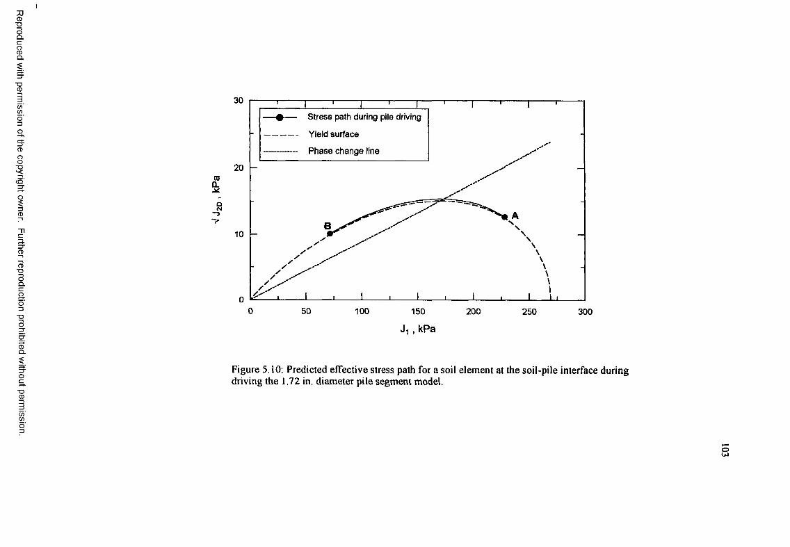
Reproduced
with perm
ission of the
copyright ow
ner. Further
reproduction prohibited
without
permission.
30
Stress path during pile driving
Yield surface
Phase change line
nCL
0 50 100 150 200 250 300
J, , kPa
Figure 5.10: Predicted effective stress path for a soil element at the soil-pile interface during driving the 1.72 in. diameter pile segment model.

Reproduced
with perm
ission of the
copyright ow
ner. Further
reproduction prohibited
without
permission.
(0Q.yU)in
in0)>'•8*=l b
150
125
100 'oo
75
50
25
0
1 10 100Normalized distance from pile wall (r/r0)
Figure 5.11: Predicted distribution of effective stresses at 16 m below the ground surface, immediately after driving 1.72 in. diameter pile segment model.
o

105
near the pile, up to a radial distance of about ten times the pile diameter. The pre
dicted effective radial stress, for example, decreased from 69 kPa before pile driving
to 17 kPa immediately after pile driving. The effective stresses in the far field re
mained under iif0-condition. A comparison of the predicted and measured effective
radial stresses immediately after driving is shown in Figure 5.12. The prediction is
consistent with the field measurements.
The proposed HiSS-^,- model successfully predicted the low stress conditions
immediately after driving. Field experiments (Earth Technology Corp., 1986; Azzouz
and Lutz, 1986; Azzouz and Morrison, 1988; Bogard and Matlock, 1990) showed that
low effective radial stresses were obtained immediately after pile driving. In a study
conducted in Empire, Louisiana, Azzouz and Lutz (1986) found that the effective
radial stresses acting on the pile shaft during installation were smaller than the
initial insitu effective radial stresses. The solution obtained in the current study is
consistent with the findings of these field studies. On the other hand, theoretical
and numerical studies (Randolph et al., 1979; Heydinger and O’Neill, 1986; Chopra
and Dargush, 1992) presented contrary results, showing that the predicted effective
radial stresses increased immediately after driving.
The predicted pore water pressure distribution and the maximum measured value
at the pile wall are shown in Figure 5.13. The maximum pore water pressure pre
dicted at the soil-pile interface was about 70% of the measured value. The maximum
excess pore water pressure was under predicted by a factor of 0.5. Similar results
were obtained by Baligh and Levadoux (1980) for cone penetrometers in clays, where
the excess pore water pressure was under estimated by a factor of 0.5. Pore water
pressure was also under predicted by a factor of 0.3 during the pile behavior study
by Wathugala (1990), where the HiSS-^J model was used to model the entire soil
domain.
Reproduced with permission of the copyright owner. Further reproduction prohibited without permission.

Reproduced
with perm
ission of the
copyright ow
ner. Further
reproduction prohibited
without
permission.
150
Field data
125 k =1.0E-8 m/sec
k=1.0E-9 m/sec
k =6.25E-10 m/sec
ro■5(0k . Immediately after
driving0)>•■83=at
25
1.0E+0 1.0E+1 1.0E+2 1.0E+3 1.0E+4
Time after pile driving, min
Figure 5.12: Comparison of predicted and measured effective radial stresses during soil consolidation around the 1.72 in. diameter pile segment model.
OC\

Reproduced
with perm
ission of the
copyright ow
ner. Further
reproduction prohibited
without
permission.
400
£3tntna>q . 200L .
B(0£2o
100
Field measurement
Finite element prediction
1 10 100
Normalized distance from pile wall (r/r0)
Figure 5.13: Predicted distribution of pore water pressure immediately after driving 1.72 in. pile segment model.
o

108
For given boundary conditions, many possible stress fields satisfy the equilib
rium requirements. In the simulation of pile driving, the analysis began with an
approximate solution for effective stresses, strains, and displacements in order to
calculate the stress field under equilibrium. The results of this analysis showed that
the calculated effective stresses are consistent with the measured values. Therefore,
the predicted effective stresses obtained by the constitutive model are the correct
effective stress fields. In such condition, many combinations of the to tal stresses and
pore water pressures can produce one effective stress field. In this method, the pore
water pressures were under predicted, and therefore the total stresses were also under
predicted.
The preceding results and discussion indicate that even though the pore water
pressure is under predicted, the effective radial stress at the end of driving is in good
agreement with the field measurement. The comparison is shown in Figure 5.12 (the
value correspond ing to coefficient of permeability k = 1 x 10~9 m/sec).
5.5 Consolidation and P ile Load Tests
The finite element simulation was conducted using the nonlinear transient analysis in
ABAQUS. The initial conditions required to start the simulation of the consolidation
phase were obtained from the end of pile driving stage. These conditions included
the pore water pressure and effective stresses distributions which were already under
equilibrium, in addition to the hardening parameters and other state dependent
variables.
During the simulation of the consolidation phase, different pile load tests (ten
sion, compression, and cyclic) were numerically simulated according to the sequence
presented in Figure 5.14. Pile load tests were conducted at degrees of consolidation
of 22, 40, 60, 87, 97, 98, and 99 percent.
Reproduced with permission of the copyright owner. Further reproduction prohibited without permission.

109
Perform static tension test at U=60%
Perform static tension test at U=98%
Perform static tension test at U=97%
Perform static tension test at U=87%
Perform static tension test at U=40%
Perform static compression test at U=97%
Perform final two-way cyclic load tests at U=99%
Install 1.72 in. full displacement pile segment model
Perform static tension test at degree o f consolidation, U=22%
Figure 5.14: Sequence o f the load tests conducted during soil consolidation around the 1.72 in. diameter pile segment model.
Reproduced with permission of the copyright owner. Further reproduction prohibited without permission.

110
The coefficient of permeability, k, was evaluated for Sabine clay, based on three
one-dimensional consolidation tests performed by the Earth Technology Corp. (1986).
In the present study, k was calculated as 6.25 xlO -10 m/sec and was used in the sim
ulation of the consolidation. The simulation was repeated using two other values for
the coefficient of permeability: 1.0xlO -8 and 1.0 xlO -9 m/sec. The eifect of k on
the rate of dissipation of the excess pore water pressure is illustrated in Figure 5.15.
The results indicate that when k equals 1.0 xlO -9 cm/sec, the predictions and field
measurements are consistent. Moreover, this value for k predicts the effective radial
stress distribution during the consolidation very well, as shown in Figure 5.12.
Using the o n e -d im ensional consolidation test, the evaluation of the coefficient of
permeability is only approximate. In the field, more reliable techniques usually axe
utilized to evaluate the coefficient of permeability. Because of the uncertainty in
evaluating k and because the difference between the calculated and corrected k is
relatively small, it is believed that the correction is within acceptable deviation. In
this study, therefore, the k value of 1.0xlO -9 m/sec was used in the simulation. This
value was also used in Chapters 6 and 7 for the closed-ended and open-ended piles,
where the results were found to be consistent with field measurements.
During the consolidation phase, the excess pore water pressures were gradually
dissipated. This dissipation was associated with the increase in the effective stresses.
The predicted pore water pressure distributions at different time intervals during
consolidation are shown in Figure 5.16. The corresponding changes in the effective
radial stresses are presented in Figure 5.17. At the end of consolidation, the excess
pore water pressures were fully dissipated and the m axim um increase in the effec
tive stresses was reached. Figure 5.18 shows the predicted variation of the effective
stresses at the completion of the consolidation. Examination of the figure indicates
that the effective radial stress increased from 17 kPa immediately after driving to
97 kPa at the end of consolidation. Moreover, the effective radial stress increased
Reproduced with permission of the copyright owner. Further reproduction prohibited without permission.
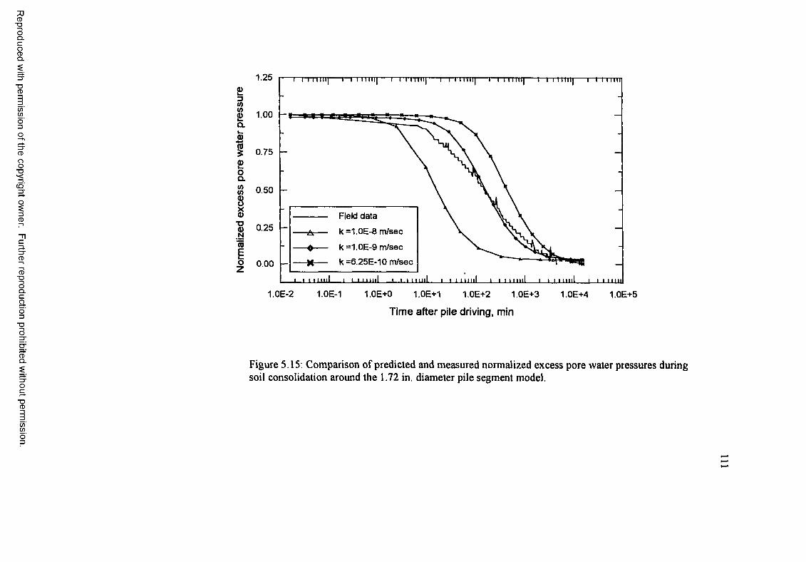
Reproduced
with perm
ission of the
copyright ow
ner. Further
reproduction prohibited
without
permission.
1.25 i n ui|£3tntn£ 1.00 -
CL
BTo£ 0.75
oQ.# 0.508 0)© 0.25N15
Field data
k =1.0E-8 m/sec
k =1.0E-9 m/sec
k =6.25E-10 m/sec§o O.oo
1.0E-2 1.0E-1 1.0E+0 1.0E+1 1.0E+2 1.0E+3 1.0E+4 1.0E+5
Time after pile driving, min
Figure 5.15: Comparison of predicted and measured normalized excess pore water pressures during soil consolidation around the 1.72 in. diameter pile segment model.

Reproduced
with perm
ission of the
copyright ow
ner. Further
reproduction prohibited
without
permission.
250 1 sec
1370 s e c
6920 secraQ. 13600 se c
22524200 se ca>
L .3Wtn 39700 sec
63100 sec
900000 sec
£a200
1(0?a)oCL
175
1501 10 100
Normalized distance from pile wall (r/r0)
Figure S. 16: Predicted dissipation of pore water pressures during soil consolidation around the 1.72 in. diameter pile segment model.

Reproduced
with perm
ission of the
copyright ow
ner. Further
reproduction prohibited
without
permission.
(0Q.j*ofo>.§u>raT>ra<u>o
HI
100 r - i - T
80
60
40
20
t--------- 1------1— i—i—r*T"T"
Q—©—©-----©—©■■ Q~^
I I _l____ I___I__I_I_I I I
— ©— 1 sec
— e — 1370 sec
-----A— 6920 sec
— B — 13800 sec
— K— 24200 sec
— ♦ — 39700 sec
-----A---- - 63100 sec
- 900000 sec
j ____ i___i__i_i_i i i1 10
Normalized distance from pile wall (r/rc)
100
Figure 5.17: Predicted increase in effective radial stresses during the consolidation of the soil around the 1.72 in. diameter pile segment m odel.
OJ

Reproduced
with perm
ission of the
copyright ow
ner. Further
reproduction prohibited
without
permission.
125
z z
(0!* 100</)'w&(Aa>>■*3uI 751U
501 10 100
Normalized distance from pile wall (r/rc)
Figure 5.18: Predicted distribution o f effective stresses at a depth o f 16 m at the end of soil consolidation around the 1.72 in. diameter pile segment model.

115
from 69 kPa before pile driving to 97 kPa at the completion of consolidation. The
effective stresses in the far field were not affected during the consolidation. The ef
fective stress path for the soil element at the soil-pile interface during consolidation
is shown in Figure 5.19. Stress point C represents the stress condition at the end of
consolidation.
The simulation of pile load tests was performed during the consolidation phase.
These tests consisted of tension pullout tests, a compression test, and the final cyclic
pile load test. The initial conditions necessary to simulate a pile load test were
obtained from the consolidation phase at a time corresponding to the degree of
consolidation at which the load test was conducted. These conditions include stresses,
pore water pressures, and hardening parameters.
The measured displacement-time history was applied to simulate the pile load
tests. In Figures 5.20, 5.21, 5.22, 5.23, 5.24, and 5.25, the finite element results
for pile load tests # 1, # 2, # 3, # 4, # 5, and # 6 are compared with the field
measurements. The shear transfer represents the average values along the shaft of the
1.72 in. diameter pile segment model. Comparisons of the predicted and measured
variations of shear transfer during these tests indicate that the simulation captured
the measured behavior very well. Predicted variations of the shear transfer with the
displacement match the measurements for pile load tests # 3, # 4 and # 6 . Other
tests showed slight differences between the predictions and measurements, but the
shear transfer values at failure were well predicted.
The predicted variations of the effective radial stresses for these tests compared
very well with the field measurements. During pile load test # 3, the estimated and
measured variations of effective radial stress contradicted each other. However, the
predicted values showed good agreement with field measurements at the beginning
and end of the test.
Reproduced with permission of the copyright owner. Further reproduction prohibited without permission.

Reproduced
with perm
ission of the
copyright ow
ner. Further
reproduction prohibited
without
permission.
Stress path during pile driving
Stress path during consolidation
Yield surface
Phase change line20(0CL
oN—i
0 50 100 150 200 250 300
Jt , KPa
Figure 5.19: Predicted effective stress path for a soil element at the soil-pile interface during pile driving and consolidation o f soil around the 1.72 in. diameter pile segment model.

Shea
r tr
ansf
er,
kPa
Shea
r tr
ansf
er,
kPa
117
20
10
0 Degree of consolidation, U = 22%
Field pile load test
Finite element simulation
-10 ----0.0E+0 3.0E-4 4.0E-4 5.0E-41.0E-4 2.0E-4
Displacement, m
(a) Shear transfer vs displacement
20
10
\ -
0 Degree of consolidation, U = 22%
Reid pile load test
Rnite element simulation
-10150 20050 1000
Time, sec
(b) Shear transfer vs time.
Figure 5.20: Comparison of predicted and measured response during pile load test #1 conducted on the 1.72 in. diameter pile segment model.
(figure con'd)
Reproduced with permission of the copyright owner. Further reproduction prohibited without permission.

Effe
ctiv
e ra
dial
str
ess,
kPa
118
40
30
20
10
00 50 100 150 200
Time, sec
(c) Effective radial stress vs time.
400
coa.
| 300(/)(0d>wQ.wd)$ 200©k .o0.
1000 50 100 150 200
Time, sec
(d) Pore water pressure vs time.
Degree of consolidation, U = 22%
Field pile load test
Rnite element simulation
A
Degree of consolidation, U = 22%
Field pile load test
Finite element simulation
Reproduced with permission of the copyright owner. Further reproduction prohibited without permission.

Shea
r tr
ansf
er,
kPa
Shea
r tr
ansf
er,
kPa
20
15
10
5
Degree of consolidation, U = 40%
Field pile load test
Finite element simulation
I I3.5E-4 4.0E-4 4.5E-4
Displacement, m
5.0E-4 5.5E-4
(a) Shear transfer vs displacement
20
15
10
Degree of consolidation, U = 40%
5 Field pile load test
Finite element simulation
025 50 750 100 125
Time, s e c
(b) Shear transfer vs time.
Figure 5.21: Comparison of predicted and measured response during pile load test #2 conducted on the 1.72 in. diameter pile segment model.
(figure con'd)
Reproduced with permission of the copyright owner. Further reproduction prohibited without permission.

Effe
ctiv
e ra
dial
str
ess,
kPa
120
e>u - i | i | 1 ~ T " i 1 1 1 1
50 — —
-
40 —
Degree of consolidation, U = 40%30 —
---------- Field pile load test—
---------- Finite element simulation -
20 1 , 1 1 . , 1 , 1
0 20 40 60 80 100 120
Time, se c
(c) Effective radial stress vs time.
1------r
raQ.
s3W(/)d)
300 -
® 200 09 $£oCL
10020
Degree of consolidation, U = 40%
Field pile load test
Finite element simulation
_L _L40 60
Time, sec
80 100 120
(d) Pore water pressure vs time.
Reproduced with permission of the copyright owner. Further reproduction prohibited without permission.

Shea
r tr
ansf
er,
kPa
Shea
r tr
ansf
er,
kPa
12140
Degree of consolidation, U = 60%
Reid pile load test
Rnite element simulation
30
20
10
0
4.0E-40.0E+0 8.0E-4 1.2E-3
Displacement, m
(a) Shear transfer vs displacement
40
Degree of consolidation, U = 60%
Field pile load test
Finite element simulation
50 750 25 100
Time, sec
(b) Shear transfer vs time.
Figure 5.22: Comparison of predicted and measured response during pile load test #3 conducted on the 1.72 in. diameter pile segment model.
(figure con'd)
Reproduced with permission of the copyright owner. Further reproduction prohibited without permission.

Pore
w
ater
pre
ssur
e, k
Pa
Effe
ctiv
e ra
dial
str
ess,
kPa
122
100
75
50
Degree of consolidation, U = 60%25 Field pile load test
Finite element simulation
00 20 40 60 80 100
Time, se c
(c) Effective radial stress vs time.
300
250 -_r
200 -
150 -Degree of consolidation, U = 60%
Field pile load test
Finite element simulation
100 I I20 40 60
Time, sec
80 100
(d) Pore water pressure vs time.
Reproduced with permission of the copyright owner. Further reproduction prohibited without permission.
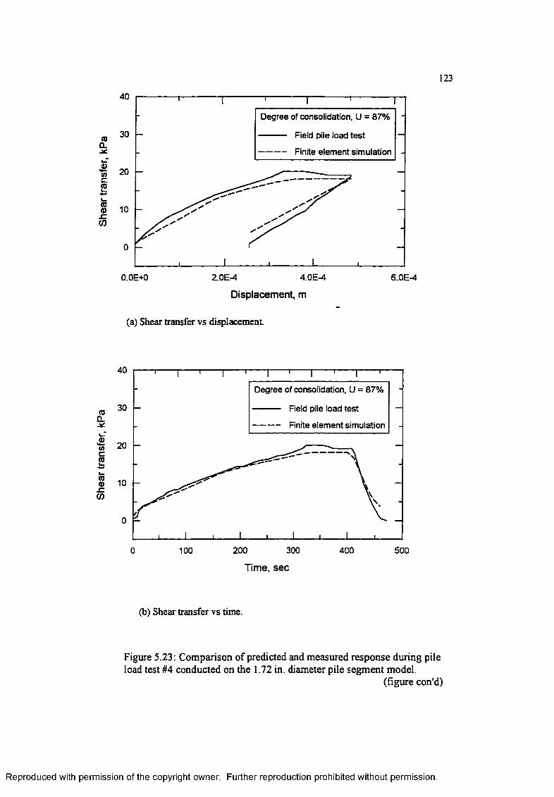
Shea
r tr
ansf
er,
kPa
Shea
r tr
ansf
er,
kPa
123
40
Degree of consolidation, U = 87%
30 Field pile load test
Finite element simulation
20
10
0
4.0E-42.0E-40.0E+0
Displacement, m
(a) Shear transfer vs displacement
40
Degree of consolidation, U = 87%
30 Reid pile load test
Rnite element simulation
20
10
0
300200 400 5000 100
Time, sec
(b) Shear transfer vs time.
Figure 5.23: Comparison of predicted and measured response during pile load test #4 conducted on the 1.72 in. diameter pile segment model.
(figure con'd)
Reproduced with permission of the copyright owner. Further reproduction prohibited without permission.

124
120
(0CLJCto'to0)L _
toro~o5©>o!fcUJ
80
40
i |" . ------- -t- " t i i
1uu— nil— |
\\ ^
-V_____S
-
- Degree of consolidation, U = 87% —
---------- Field pile load test
---------- Finite element simulation
> 1 i 1 1 , 1 ,
100 200 300
Time, se c
400 500
(c) Effective radial stress vs time.
300
(00.
| 200toto©
©ro
£o0.
100 - Degree of consolidation, U = 87%
Field pile load test
Finite element simulation
100 200 300
Time, se c
400 500
(d) Pore water pressure vs time.
Reproduced with permission of the copyright owner. Further reproduction prohibited without permission.

Shea
r tr
ansf
er,
kPa
Shea
r tr
ansf
er,
kPa
125
30
20
10
Degree of consolidation, U =97%
0 Field pile load test
Finite element simulation
-10 ----0.0E+0 4.5E-3 6.0E-33.0E-31.5E-3
Displacement, m
(a) Shear transfer vs displacement.
30
20
10
Degree of consolidation, U = 97%
0 Field pile load test
Finite element simulation
-10200 250 30050 100 1500
Time, sec
(b) Shear transfer vs time.
Figure 5.24: Comparison of predicted and measured response during pile load test #5 conducted on the 1.72 in. diameter pile segment model.
(figure con'd)
Reproduced with permission of the copyright owner. Further reproduction prohibited without permission.

Pore
w
ater
pre
ssur
e, K
Pa
Effe
ctiv
e ra
dial
str
ess,
kPa
126
300
Degree of consolidation, U = 97%
Field pile load test
Finite element simulation200
100 2000 300
Time, se c
(c) Effective radial stress vs tune.
r—200
100
Degree of consolidation, U = 97%
Field pile load test
Finite element simulation
00 100 200 300
Time, se c
(d) Pore water pressure.
R eproduced with perm ission of the copyright owner. Further reproduction prohibited without perm ission.

Shea
r tr
ansf
er,
KPa
Shea
r tr
ansf
er,
kPa
30
Degree of consolidation, U = 97%
Reid pile load test
Rnite element simulation15
0
-15
-30 ------3.2E-3 -2.4E-3 -1.6E-3 -8.0E-4 0.0E+0
Displacement, m
(a) Shear transfer vs displacement
30
Degree of consolidation, U = 97%
Field pile load test15
Rnite element simulation
0
-15
-30400 6000 200 800 1000
Time, s e c
(b) Shear transfer vs time.
Figure 5.25: Comparison of predicted and measured response during pile load test #6 conducted on the 1.72 in. diameter pile segment model.
(figure con'd)
Reproduced with permission of the copyright owner. Further reproduction prohibited without permission.

Pore
w
ater
pre
ssur
e, k
Pa
Effe
ctiv
e ra
dial
str
ess,
kPa
128
100
75
50
Degree of consolidation, U = 97%25 Field pile load test
Finite element simulation
0400 600 800 10002000
Time, sec
(c) Effective radial stress vs time.
200 -
'--------------- j
100 -
Degree of consolidation, U = 97%
Field pile load test
Finite element simulation
200 400 600
Time, sec
800 1000
(d) Pore water pressure vs time.
Reproduced with permission of the copyright owner. Further reproduction prohibited without permission.

129
Since the pore water pressure was underestimated at the end of pile driving, the
discrepancy occurred in the first few pile load tests. Comparisons of the measured
and predicted changes in the pore water pressure during pile load tests # 4, # 5,
and # 6 indicate that the results are not consistent with each other. Generally, the
pore water pressure is not predicted well in this study.
Pile load test # 7 was numerically simulated at a degree of consolidation of
98 percent. Loading-unloading cycles were performed during the test. The finite
element results, as compared to the field measurements, are depicted in Figure 5.26.
The predicted variations of the shear transfer during the test are in good agreement
with field measurements, as shown in Figures 5.26a and 5.26b. The predictions
accurately capture the behavior during the loading-unloading cycles. Variations of
predicted effective radial stresses and pore water pressures are consistent with field
measurements (Figures 5.26c and 5.26d).
The final two-way cyclic load test was conducted near the end of consolidation.
The test consisted of five tension-compression cycles. During all cycles, the failure
occurred before the direction of loading was reversed. A comparison of the predicted
and measured shear transfer variations with displacement is shown in Figure 5.27.
The simulation predicted the response during the first cycle very well. During the
other cycles, the estimated shear transfer was slightly lower than that of the field
measurements. The variation of shear transfer during the test is presented in Figure
5.28. The predicted and measured response are in good agreement. The variations
with time of the effective radial stress and pore water pressure are shown in Figures
5.29a and 5.29b, respectively. The variations in the predicted effective radial stress
and pore water pressure during the test were relatively smaller than those in the
measured values. However, the finite element results at the beginning and end of the
test aue in good agreement with the field measurements.
Reproduced with permission of the copyright owner. Further reproduction prohibited without permission.

Shea
r tr
ansf
er,
kPa
Shea
r tr
ansf
er,
kPa
130
40
20
0
-20Degree of consolidation, U = 98%
Reid pile load test
Rnite element simulation
-40
-60 -----0.0E+0 1.5E-35.0E-4 1.0E-3 2.0E-3
Displacement, m
(a) Shear transfer vs displacement
40
20
0
-20Degree of consolidation, U = 98%
Field pile load test-40
Finite element simulation
-60200 400 600 8000 1000
Time, sec
(b) Shear transfer vs time.
Figure 5.26: Comparison of predicted and measured response during pile load test #7 conducted on the 1.72 in. diameter pile segment model.
(figure con'd)
Reproduced with permission of the copyright owner. Further reproduction prohibited without permission.

Pore
w
ater
pre
ssur
e, k
Pa
Effe
ctiv
e ra
dial
str
ess,
kPa
131
100
75
" \
50
Degree of consolidation, U = 98%
25 Reid pile load test
Rnite element simulation
4000 200 600 800
Time, se c
(a) Effective radial stress vs time.
250
200
150 Degree of consolidation, U = 98%
Field pile load test
Finite element simulation
1000 200 400 600 800
Time, se c
(b) Pore water pressure vs time.
Reproduced with permission of the copyright owner. Further reproduction prohibited without permission.
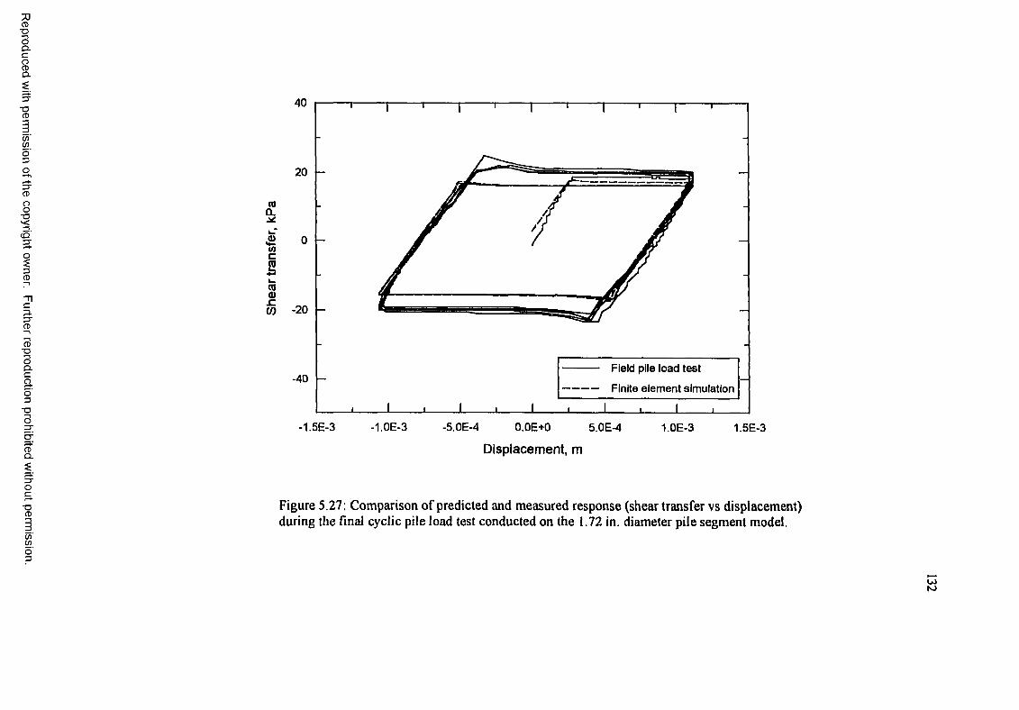
Reproduced
with perm
ission of the
copyright ow
ner. Further
reproduction prohibited
without
permission.
40
20
coQ.Mil> owc£L .
W -20
-40
-1.5E-3 -1.0E-3 -5.0E-4 0.0E+0 5.0E-4 1.0E-3 1.5E-3
Displacement, m
Figure 5.27, Comparison of predicted and measured response (shear transfer vs displacement) during the final cyclic pile load test conducted on the 1.72 in. diameter pile segment model.
T
Field pile load test
Finite element simulation
J i I i I ■ I ■ I
u>K>

Reproduced
with perm
ission of the
copyright ow
ner. Further
reproduction prohibited
without
permission.
40
20
-V
(0c£&_CO0)JC0)
-20
Field pile load test
Finite element simulation-40
2000 400 600 800 1000 1200
Time, sec
Figure 5.28: Comparison of predicted and measured response (shear transfer vs time) during the final cyclic pile load test conducted on the 1.72 in. diameter pile segment model.
U>U>

134
200
Field pile load test
Finite element simulation(0CL
150(003
2•*4CO
m 100■o5a)> ” \o:t=III
4000 800 1200
Time, sec
(a) Effective radial stress vs time.
250
(0CL- * 200
3C/303
Q. 150k .0)+-»CD
50)u . 100 - Field pile load test
Finite element simulationoCL
4000 800 1200
Time, sec
(b) Pore water pressure vs time.
Figure 5.29: Comparison of predicted and measured response during the final cyclic pile load test conducted on the 1.72 in. diameter pile segment model.
Reproduced with permission of the copyright owner. Further reproduction prohibited without permission.

135
5.6 P ile Setup
The main objective of the current research was to predict pile setup, or the increase
of bearing capacity with time after pile driving. In order to accomplish this task,
the finite element simulation of pile load tests during consolidation was conducted.
Comparisons of the predicted and measured behavior of the pile in these tests showed
that the finite element results are in good agreement with field measurements.
For some load tests, the finite element simulation accurately predicted the mea
sured shear transfer at failure. For each simulated pile load test, the estimated peak
and residual shear transfer values were compared with those obtained in the field.
The results are presented in Figure 5.30. The comparisons showed that the predicted
increase in the shear transfer with time after pile driving are consistent with the field
measurements.
It should be noted that at the beginning of consolidation, the finite element
method overestimated the pile setup. The reason could be that the constitutive
model is not calibrated using overconsolidated test data. The finite element method
underpredicted pile setup at the end of soil consolidation.
Reproduced with permission of the copyright owner. Further reproduction prohibited without permission.

Reproduced
with perm
ission of the
copyright ow
ner. Further
reproduction prohibited
without
permission.
(0Q.i_ra(ACroL -(0a>JC(0
30
20
Field test, peak10
Field test, residual
— A -— Prediction, peak
— ©•— Prediction, residual
0 — 1.0E+3 1.0E+4 1.0E+5
Time after pile driving, sec
Figure 5.30; Comparison of predicted and measured increase in soil-pile shear transfer at failure (skin friction) for pile load tests performed at different time periods after driving.
U>O s

CHAPTER 6 NUMERICAL SIMULATION OF THE
BEHAVIOR OF CLOSED-ENDED PILES
6.1 Introduction
In the previous chapter, a proposed numerical method for investigating the increase in
bearing capacity, with time, of friction piles driven into saturated clay, was verified
with respect to field experiments. The proposed HiSS-^i model was calibrated
and successfully predicted the soil behavior at Sabine Pass, Texas. Then numerical
simulations of pile driving, subsequent consolidation, and load tests were conducted.
The numerical results were verified with respect to the field experiments conducted
on the 1.72 in. diameter pile segment model. During the verification stage, material
parameters, soil conditions, and numerical stability and convergence parameters for
Sabine clay were identified. It was essential to utilize this numerical environment to
evaluate another set of field experiments. The back prediction scheme would support
and assure the validity of the method.
The main objective of the current research was to study the increase in the
shaft capacity, with time, of friction piles driven into saturated clay. Therefore,
finite element numerical simulations of the different load tests conducted during
consolidation on the 3 in. diameter pile segment model, were employed to achieve
this goal. These load tests provided the qualitative and quantitative estimates of the
time increase in shaft capacity (or pile setup).
This chapter presents the results of the numerical simulation of the various life
stages of a closed-ended pile segment model driven into saturated clay.
137
Reproduced with permission of the copyright owner. Further reproduction prohibited without permission.

138
6.2 Field Experim ents
Field experiments on a 3 in. diameter pile segment model were conducted during the
Earth Technology Corp. investigation (1986). The experiments consisted of measur
ing the total radial pressure, pore water pressure, shear transfer, and relative soil-pile
displacement, during driving, consolidation, and load testing. The 3 in. diameter
pile segment model was installed according to the procedure described in Figure 5.1
(refer to Section 5.2). Figure 6.1 presents the variations in the measured total radial
and pore water pressures as well as the change in the corresponding effective radial
pressure during consolidation. During consolidation, a series of pile load (tension
and cyclic) tests were conducted at different time intervals corresponding to degrees
of consolidation of 18, 37, 92, and 100 percent. Figure 6.2 shows the variation of the
shear transfer with the displacement for the conducted tension pile load tests. The
final two-way cyclic pile load test was performed at the completion of consolidation.
Figure 6.3 displays the sequence of these tests.
6.3 Finite Elem ent M esh
The 8-node axisymmetric solid element CAX8RP was used in the finite element
analysis (the element and its properties were described in Section 5.3.3).
The soil mass was discretized according to the finite element mesh presented in
Figure 6.4. The mesh consisted of 578 elements and 1837 nodes. The described mesh
(Figure 6.4) was used for the finite element simulation of consolidation and pile load
tests. The soil mass surrounding the pile was modeled as the HiSS-tfJi material.
Reproduced with permission of the copyright owner. Further reproduction prohibited without permission.

Effe
ctiv
e ra
dial
pre
ssur
e, k
Pa
Tota
| ra
dia|
and
po
re
pres
sura
kP
a139
400
300
200 -Total radial pressure
Pore water pressure
10010 100 10001 10000
Time after driving, min
(a) Total radial and pore water pressures.
100
50
10 1001 1000 10000
Time after driving, min
(b) Effective radial pressure.
Figure 6.1: Variation of the measured pressures during soil consolidation around the 3 in. diameter pile segment model (after Earth Technology Corp., 1986).
Reproduced with permission of the copyright owner. Further reproduction prohibited without permission.

Reproduced
with perm
ission of the
copyright ow
ner. Further
reproduction prohibited
without
permission.
30
20
CD0 .
&tncs
\
I—(0a)szCO U = 18%
U - 37%
U = 92%-10 U = 100%
5.0E-40.0E+0 1.0E-3 1.5E-3 2.0E-3 2.5E-3
Displacement, m
Figure 6.2: Results of static tension tests conducted on the 3 in. diameter pile segment model (after Earth Technology Corp., 1986).
O

141
Perform static tension test at U=92%
erform static tension test at U=100
Perform static tension test a t U=37%
Install 3 in. full displacement pile segment model
Perform final two-way cyclic load test at U=100%
Perform static tension test at degree o f consolidation, U=18%
Figure 6.3: Sequence o f the load tests conducted during soil consolidation around the 3 in. diameter pile segment model.
Reproduced with permission of the copyright owner. Further reproduction prohibited without permission.

142
s >
§ >
S > ,
T
< 5
aA
Element &-node ABAQUS-CAX8RP 578 elements 1837 nodes
Figure 6.4: The finite element mesh used to discretize the soil domain around the 3 in. diameter pile segment model.
Reproduced with permission of the copyright owner. Further reproduction prohibited without permission.

143
6.4 Pile Driving
The 3 in. diameter pile segment model was driven according to the procedure de
scribed in Figure 5.1. The simple pile approach (Baligh, 1984), developed for deep
penetration of closed-ended piles, was utilized to obtain the strain field in the soil
during pile driving (details of this subject were described in Section 4.3). Simulation
of pile driving was performed in a manner similar to the simulation of the 1.72 in
diameter pile segment model (Section 5.4).
Throughout this chapter (unless otherwise indicated), the numerical results for
the soil element located at the soil-pile interface at 16 m below ground surface, are
compared with field measurements. This depth (16 m) corresponds to the approxi
mate location of the total and pore water pressure transducers during testing.
The predicted effective stress path for the soil element at the soil-pile interface
during driving is shown in Figure 6.5. Points A and B represent the initial K a-
condition before, and the condition immediately after pile driving, respectively. In
this study, simulation of pile driving reduced the effective mean stress (J i/3 ) as well
as the second invariant of the deviatoric stress tensor {Jzd)- At the end of driving,
the effective stresses for the soil around the pile were substantially decreased. On
the other hand, the effective stresses for the soil in the far field remained under K a-
conditions. Examination of Figure 6.6 indicates that the decrease in the predicted
effective stresses around the pile extended to about ten times the pile diameter. The
effective radial stress decreased from 70 kPa before, to 18 kPa immediately after pile
driving. The prediction of low effective radial stress at the end of pile installation
is consistent with the field measurements (Figure 6.7). The predicted pore water
pressure distribution at the end of pile driving is depicted in Figure 6 .8 . Shown
in the same figure is the measured pore water pressure, at the soil-pile interface,
immediately after pile driving. The numerical simulation predicted about 66% of
Reproduced with permission of the copyright owner. Further reproduction prohibited without permission.

Reproduced
with perm
ission of the
copyright ow
ner. Further
reproduction prohibited
without
permission.
30
Stress path during pile driving
Yield surface
Phase change line20
toQ.
Q04—)
0 100 200 300
J , , kPa
Figure 6.5: Predicted effective stress path for a soil element at the soil-pile interface during driving 3 in. diameter pile segment model.
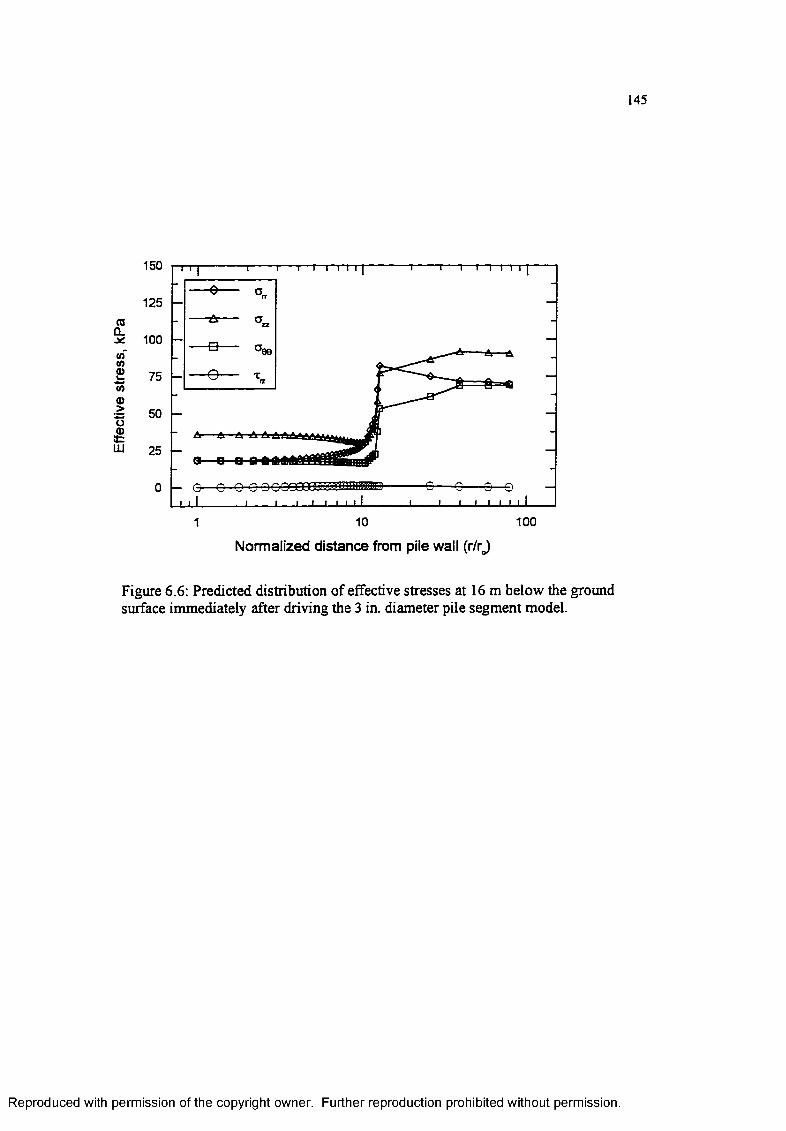
Effe
ctiv
e st
ress
, K
Pa145
150
125
100
75
50
25
0
Figure 6 .6 : Predicted distribution of effective stresses at 16 m below the ground surface immediately after driving the 3 in. diameter pile segment model.
A A A A A .
G—G C O QQQQG8E
1 10 100
Normalized distance from pile wall (r/rj
Reproduced with permission of the copyright owner. Further reproduction prohibited without permission.

Reproduced
with perm
ission of the
copyright ow
ner. Further
reproduction prohibited
without
permission.
125
Field data
k =1.0E-8 m/sec(0 100 Q.
k=1.0E-9 m/secminSinTo
k =6.25E-10 m/sec
T32 After driving50a>>'Sa=LU
i 11ill i i m il___
1.0E+41.0E-1 1.0E+0 1.0E+1 1.0E+2 1.0E+3
Time after pile driving, min
Figure 6.7: Comparison of predicted and measured effective radial stresses after driving, and during soil consolidation around the 3 in. diameter pile segment model.
-u0\

Reproduced
with perm
ission of the
copyright ow
ner. Further
reproduction prohibited
without
permission.
300
Finite element prediction
Field measurementtoQ.
O. 200
OCL
1001 10 100
Normalized distance from pile wall (r/r0)
Figure 6.8: Predicted distribution of pore water pressure immediately after driving 3 in. diameter pile segment model.
4*."4

148
the maximum pore water pressure measured at the pile wall. The maximum excess
pore water pressure was underestimated by a factor of 0.41. The maximum pore
water pressure was underestimated by a factor of 0.5 in the case of the 1.72 in.
diameter pile segment model (Chapter 5).
6.5 Consolidation and Pile Load Tests
The finite element simulation of the subsequent consolidation and load tests was
conducted according to the same procedure used for the X-probe in Chapter 5. Fig
ure 6.3 shows the sequence of simulating the pile load tests during the consolidation
phase.
The predicted and measured effective radial stresses during consolidation are com
pared in Figure 6.7. The finite element results indicate that the simulation predicted
the field behavior very well. The analysis was performed with the calibrated value
of the coefficient of permeability (k = 1 x 10⁻⁹ m/sec). This comparison supports
the argument presented in Section 5.2 regarding the coefficient of permeability.
During consolidation, the effective stresses gradually increased as the excess pore
water pressures dissipated. A comparison of the predicted and measured normalized
excess pore water pressures is presented in Figure 6.9. The numerical results are in
good agreement with the field measurements, and the pattern of the measured dis
sipation is accurately estimated. Most of the excess pore water pressures dissipated
within three hours after driving. The predicted pore water pressure distributions
at different time periods during consolidation are shown in Figure 6.10. The corre
sponding estimated increase in the effective radial stresses is depicted in Figure 6.11.
At the end of consolidation, the maximum increase in the effective stresses devel
oped upon complete dissipation of the excess pore water pressures (Figure 6.12). The
Reproduced with permission of the copyright owner. Further reproduction prohibited without permission.

Reproduced
with perm
ission of the
copyright ow
ner. Further
reproduction prohibited
without
permission.
1.25
3inw£ 1.00Q.
0.75
o0.50
inina>oa> 0.25
T 3<UN0.00
Field data
k=1.0E-8 m/sec
k=1.0E-9 m/sec(0EU . k =6.25E-10 m/secoz xuJ_
1.0E+4-0.25
1.0E+0 1.0E+1 1.0E+2 1.0E+3
Time after pile driving, min
Figure 6.9: Comparison of predicted and measured normalized excess pore water pressures during soil consolidation around the 3 in. diameter pile segment model.

Reproduced
with perm
ission of the
copyright ow
ner. Further
reproduction prohibited
without
permission.
fljQ_
e3(0Wa>
£CO
£oOu
250
11 sec
74 sec225
290 sec
1154 sec
4610 sec200
38434 se c
178434 sec
900000 sec175
O Q OOOQi
1501 10 100
Normalized distance from pile wall (r/rQ)
Figure 6.10. Predicted distribution o f pore water pressures during consolidation o f the soil around the 3 in. diameter pile segment model.
L/iO
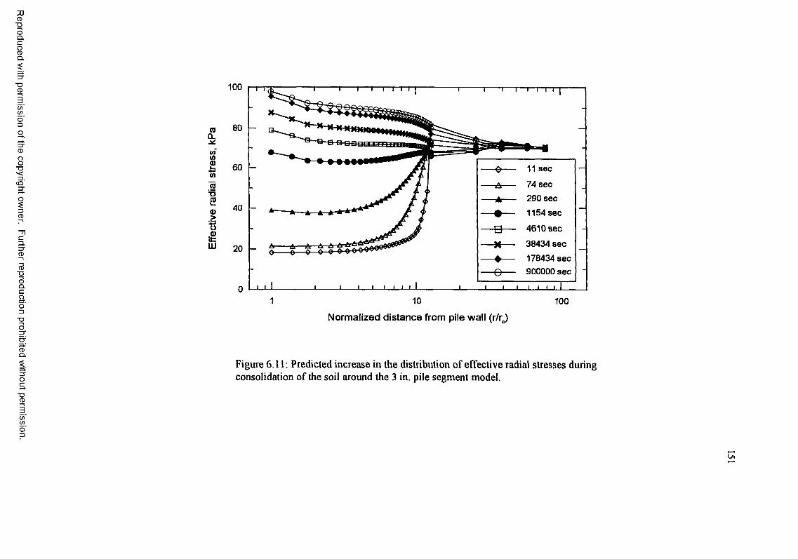
Reproduced
with perm
ission of the
copyright ow
ner. Further
reproduction prohibited
without
permission.
n>CLXLin(/>0)-bV)raTJ2a>>'■8i»=ID
100
80
60 11 sec
74 sec 290 sec
1154 sec40
4610 sec
38434 sec
178434 se c 900000 se c
20
01 10 100
Normalized distance from pile wall (r/r0)
Figure 6.11: Predicted increase in the distribution of effective radial stresses during consolidation of the soil around the 3 in. pile segment model.
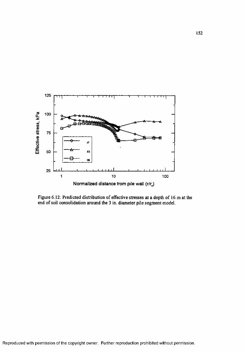
Effe
ctiv
e st
ress
, kP
a152
125
100
75
50
251 10 100
Normalized distance from pile wall (r/ro)
Figure 6.12: Predicted distribution of effective stresses at a depth of 16 m at the end of soil consolidation around the 3 in. diameter pile segment model.
Reproduced with permission of the copyright owner. Further reproduction prohibited without permission.

153
predicted effective radial stress increased from 18 kPa immediately after driving to
98 kPa at the end of consolidation. The final estimated effective stresses near the pile
increased when compared with the pre-driving conditions (ifo-conditions). For ex
ample, the predicted effective radial stress increased from 70 kPa before pile driving
(iT0-condition), to 98 kPa at the end of consolidation. In the far field, on the other
hand, the effective stresses of the soil remained unchanged during consolidation.
The predicted effective stress path during consolidation for the soil element at the
soil-pile interface is shown in Figure 6.13. Point C represents the stress condition at
the end of consolidation.
Four static tension pile load tests were simulated during the consolidation phase.
In addition, a simulation of the final two-way cyclic load test was conducted at the
end of consolidation (Figure 6.3).
The first three static pile load tests were performed in the tension mode. These
tests were simulated at degrees of consolidation of 18, 37, 92, and 100 percent.
Comparisons of predicted and measured response during pile load tests # 1, # 2, and
# 3 axe shown in Figures 6.14, 6.15, and 6.16, respectively. Changes in predicted
shear transfer during these tests are consistent with field measurements (Figures
6.14a, 6.14b, 6.15a, 6.15b, 6.16a and 6.16b). It should be noted that the shear transfer
is the average value along the shaft of the pile segment model. The estimations
of shear transfer at failure were successfully achieved. The predicted changes in
the effective radial stresses compare well with the measured changes (Figures 6.14c,
6.15c, 6.16c).
The estimated pore water pressure variations together with the field measure
ments zire presented in Figures (6.14d, 6.15d, 6.16d). Because of the difference be
tween the measured and predicted pore water pressures immediately after driving,
pore water pressures were predicted less than the measured values during tests #
Reproduced with permission of the copyright owner. Further reproduction prohibited without permission.

Reproduced
with perm
ission of the
copyright ow
ner. Further
reproduction prohibited
without
permission.
(0Q.
QCM—}
V
30
Stress path during pile driving (A-B)
Stress path during consolidation (B-C)
Yield surface
Phase change line20
10
00 100 200 300
J i , kPa
Figure 6.13: Predicted effective stress path for a soil element at the soil-pile interface during driving and soil consolidation around the 3 in. diameter pile segment model.
L/i
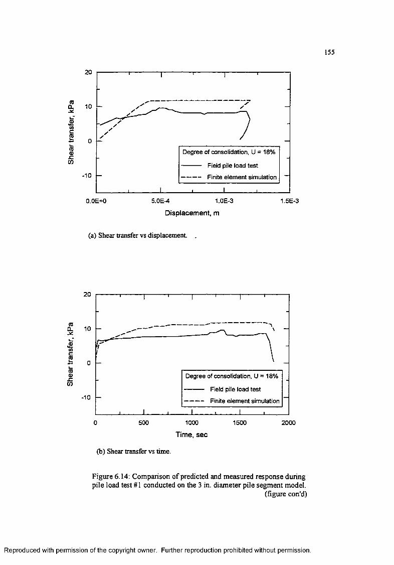
Shea
r tr
ansf
er,
kPa
Shea
r tr
ansf
er,
kPa
155
20
10
0Degree of consolidation, U = 18%
Field pile load test
Finite element simulation-10
5.0E-4 1.0E-3 1.5E-3O.OE+O
Displacement, m
(a) Shear transfer vs displacement
20
10
0
Degree of consolidation, U = 18%
Field pile load test
Finite element simulation-10
5000 1000 1500 2000
Time, sec
(b) Shear transfer vs time.
Figure 6.14: Comparison of predicted and measured response during pile load test #1 conducted on the 3 in. diameter pile segment model.
(figure con'd)
Reproduced with permission of the copyright owner. Further reproduction prohibited without permission.

156
40
(0a.
mtna>L -<n
20
©>o!t=LU
Degree of consolidation, U = 18%
Field pile load test
Finite element simulation
0 500 15001000 2000
Time, s e c
(c) Effective radial stress vs time.
400
CD£L
| 300COCO0)L .Q.k -0)I 200Soa.
1000 500 1000 1500 2000
Time, se c
(d) Pore water pressure vs time.
Degree of consolidation, U = 18%
Field pile load test
Finite element simulation
Reproduced with permission of the copyright owner. Further reproduction prohibited without permission.

157
coCLJC
UicCOL_
1 -COa>szCO
[Degree of consolidation, U=37%
Field pile load test
Finite element simulation-10
O.OE+O 5.0E-4 1.0E-3 1.5E-3
Displacement, m
(a) Shear transfer vs displacement
coo.
aincCO
CO0)JZCO
Degree of consolidation, U = 37%
Reid pile load test
Rnite element simulation-10
200 40 60 80 100
Time, se c
(b) Shear transfer vs time.
Figure 6.15: Comparison of predicted and measured response during pile load test #2 conducted on the 3 in. diameter pile segment model.
(figure con'd)
Reproduced with permission of the copyright owner. Further reproduction prohibited without permission.

Effe
ctiv
e ra
dial
str
ess,
kPa
158
60
40
20 Degree of consolidation, U = 37%
Field pile load test
Finite element simulation
00 20 40 60 80 100
Time, sec
(c) Effective radial stress vs time.
coO.
23U]in<o
d>(05£oQ.
300 = -
200 -
100 -
20
Degree of consolidation, U = 37%
Reid pile load test
Rnite element simulation
_L40 60
Time, sec
80 100
(d) Pore water pressure vs time.
Reproduced with permission of the copyright owner. Further reproduction prohibited without permission.

Shea
r tr
ansf
er,
kPa
Shea
r tr
ansf
er,
kPa
159
30
20
10
Degree of consolidation, U = 92%0
Field pile load test
Finite element simulation-10
0.0E+0 5.0E-4 1.0E-3 1.5E-3 2.0E-3 2.5E-3
Displacement, m
(a) Shear transfer vs displacement
30
20
10
0
Degree of consolidation, U = 92%
-10 Field pile load test
Finite element simulation
-202000 400 600 800 1000
Time, se c
(b) Shear transfer vs time.
Figure 6.16: Comparison of predicted and measured response during pile load test #3 conducted on the 3 in. diameter pile segment model.
(figure con'd)
Reproduced with permission of the copyright owner. Further reproduction prohibited without permission.

Pore
w
ater
pre
ssur
e, k
Pa
Effe
ctiv
e ra
dial
str
ess.
kPa
160
120
80
Degree of consolidation, U = 92%
Field pile load test
Finite element simulation
40
0 200 400 600 800
Time, se c
(c) Effective radial stress vs time.
3UU "■ ' I ' I 1 1 1
✓ \200 —
____________
100 Degree of consolidation, U = 92%
---------- Field pile load test
---------- Finite element simulation -
0 1 , 1 1
0 200 400 600 800
Time, sec
(d) Pore water pressure vs time.
Reproduced with permission of the copyright owner. Further reproduction prohibited without permission.

161
1 and # 2. However, the simulation predicted the correct trend of the pore water
pressure change during these tests.
Pile load test # 4 was simulated at the completion of consolidation (degree of
consolidation, U=100%). Unlike in the previous tests, loading and unloading cycles
were simulated during this test. As presented in Figures 6.17a and 6.17b, both
the predicted and measured shear transfer show consistent patterns during loading-
unloading cycles. Figure 6.17c presents the comparison between measured and pre
dicted effective radial stresses during the test. The field measurements did not show
any significant variation during the cycles of the test. The simulated results and
the field measurements diverged at the end of the test. Changes in predicted and
measured pore water pressure during the test are shown in Figure 6.17d. The results
compared well with each other.
Finally, numerical simulation was performed to predict the behavior during the
final two-way cyclic pile load test. The test consisted of five tension-compression
cycles. The numerical results are in good agreement with the measurements, as
presented in Figure 6.18. The predicted shear transfer change with displacement,
in the first tension cycle, was slightly lower than in the field measurements. As
depicted in Figure 6.18a, estimation of shear transfer during the compression part
of the cycle is consistent with field measurements. During the tension part of the
cycle, the predicted shear transfer was slightly lower than the field measurements.
However, the numerical simulation accurately captured the response patterns during
the tension-compression cycles (Figure 6.18b).
Predicted and measured variations of the effective radial stresses during the test
are compared in Figure 6.18c. Field measurements did not show a consistent behavior
during the test. The predicted results were slightly lower than the measurements.
A comparison of the predicted and measured pore water pressure during the test is
Reproduced with permission of the copyright owner. Further reproduction prohibited without permission.

Shea
r tr
ansf
er,
kPa
Shea
r tr
ansf
er,
kPa
162
40 Degree of consolidation, U = 100%
Field pile load test
Finite element simulation
8.0E-4 1.6E-3 2.4E-3O.OE+O 3.2E-3
Displacement m
(a) Shear transfer vs displacement
40 Degree of consolidation, U = 100%
Field pile load test
30 Finite element simulation
20
500 1000 15000 2000 2500
Time, s e c
(b) Shear transfer vs time.
Figure 6.17: Comparison of predicted and measured response during pile load test #4 conducted on the 3 in. diameter pile segment model.
(figure con'd)
Reproduced with permission of the copyright owner. Further reproduction prohibited without permission.

163
toQ.ininsto52©_>Oit=LU
150
100
50 -
n 1----------1----------r t r t r
Degree of consolidation, U = 100%
Reid pile load test
Finite element simulation
_■__ _______ ;— v.
V
_l_________1________ I_________L. _ l _ _ _ _ _ _ _ _ L _
500 1000 1500
Time, s e c
2000 2500
(c) Effective radial stress vs time.
300
(0CL
§ 200COCO£Q.©| 100©L _oQ.
00 500 1000 1500 2000 2500
Time, sec
(d) Pore water pressure vs time.
I\\■\\\\
I I
■> | - r | ,
“
— Degree of consolidation, U = 100% -
---------- Reid pile load test
----------Rnite element simulation
I . I I , I
Reproduced with permission of the copyright owner. Further reproduction prohibited without permission.

Reproduced
with perm
ission of the
copyright ow
ner. Further
reproduction prohibited
without
permission.
Finite element simulation
-2.0E-3 -1.0E-3 0.0E+0 1.0E-3 2.0E-3
Displacement, m
(a) Shear transfer vs displacement.
Figure 6.18: Comparison of predicted and measured response during the cyclic pile load test conducted on the 3 in. diameter pile segment model.
(figure con'd)
£

Reproduced
with perm
ission of the
copyright ow
ner. Further
reproduction prohibited
without
permission.
40
(QCL
-Stncra• tol _raa>
_ c(/)
500
I1000
Field pile load test
Finite element simulation
_ J i l i I i I__1500 2000 2500 3000
Time, sec
(b) Shear transfer vs time.

Pore
w
ater
pre
ssur
e,kP
a Ef
fect
ive
radi
al s
tres
s, k
Pa
150 Reid pile load test
Rnite element simulation
100 -
ou . / N /* l ••*'1 —l/ ' V v' \ / V i / \
» u
—1
I0 500 1000 1500 2000 2500 3000
Time, sec
(c) Effective radial stress vs time.
250
200
150 -
100 -
Field pile load test
Finite element simulation
2000500 1000 1500 2500 30000
Time, sec
(d) Pore water pressure vs time.
Reproduced with permission of the copyright owner. Further reproduction prohibited without permission.

167
depicted in Figure 6.18d. The variations of predicted pore water pressure during the
test cycles were slightly higher than field measurements.
Regardless of the slight differences between the measured and predicted responses,
the finite element simulation successfully estimated the various behavior patterns of
the field experiments.
6.6 Pile Setup
Conducting pile load tests at different time intervals during consolidation provided
the necessary means for finding the variation in pile shaft capacity with time. For
each conducted load test (field measurements and finite element simulation), the peak
and residual values of the shear transfer were identified. Figure 6.19 compares the
predicted and measured increases with time in the peak and residual shear transfer
during the pile load tests. Within the same set of measurements and predictions, the
differences between the peak and residual values were small.
The predicted peak shear transfer increased from 11 kPa, 54 minutes after driving,
to 19 kPa, at the end of consolidation. The corresponding field measurements were
increased from 10 to 24 kPa. Therefore, the increase in the shear transfer with time
occurred in both the measured and predicted results. In conclusion, even though the
simulation estimated a slightly lower setup at the end of consolidation, the predictions
compared very well with the field measurements, and both results have consistent
patterns.
Reproduced with permission of the copyright owner. Further reproduction prohibited without permission.

Reproduced
with perm
ission of the
copyright ow
ner. Further
reproduction prohibited
without
permission.
Field test, peak
Field test, residual30
— A -— Prediction, peak(0CL
— - Prediction, residual
u>c
I—(0a>xzCO
1.0E+3 1.0E+4 1.0E+5 1.0E+6
Time after pile driving, sec
Figure 6.19: Comparison o f predicted and measured increase in soii-pile shear transfer (setup) during pile load tests performed at different time periods after driving.

CHAPTER 7 NUMERICAL SIMULATION OF THE BEHAVIOR OF OPEN-ENDED PILES
7.1 Introduction
Open-ended piles are usually steel pipes or concrete cylinders. These piles are com
monly used in geotechnical and offshore engineering applications. It is essential to
study the behavior of open-ended piles in order to evaluate their response during
driving and loading.
As presented in Chapter 5 and 6 , the numerical simulation of the behavior of
closed-ended piles was successfully achieved. But the behavior of open-ended piles,
during driving and loading, differs from that of closed-ended piles. As the open-
ended pile penetrates the ground, the soil enters the pile. The accumulation of soil
inside the pile may result in pile plugging, which affects the behavior of the pile.
In this study, the method used for predicting the response of closed-ended piles
was modified for open-ended piles. This method was applied to predict the response
of field experiments (Earth Technology Corp. 1986) conducted on a 3 in. diameter
pile segment model with changeable cutting shoes, during driving, consolidation,
and load testing. The purpose of using the cutting shoes was to investigate the
behavior of open-ended piles. The numerical results were compared with the field
measurements in order to demonstrate the validity of the procedure for open-ended
piles.
This Chapter presents the results of the numerical simulation of the field exper
iments conducted on the 3 in. x 0.125 in. and 3 in. x 0.065 in. open-ended pile
segment models driven into Sabine clay.
169
Reproduced with permission of the copyright owner. Further reproduction prohibited without permission.

170
7.2 Field Experim ents
Part of the Earth Technology Corp. study (1986) was to investigate the response of
open-ended piles during driving, subsequent consolidation, and load testing. There
fore, field experiments were conducted on a 3 in. diameter pile segment model driven
with cutting shoes of 0.125 in. and 0.065 in. wall thicknesses.
Changes in the measured total radial and pore water pressures as well as in the
corresponding calculated effective radial pressure, during soil consolidation for the 3
in. x 0.125 in. and 3 in. x 0.065 in. open-ended pile segment models, are shown in
Figures 7.1 and 7.2, respectively. Earth Technology Corp. (1986) reported a leakage
of moisture during the experiment on the 3 in. x 0.125 in. model, as a result,
instability in the recorded data was observed. The incident occurred at a degree
of consolidation of 93%; thus, the loss of the pressure data did not invalidate the
experiment. In the case of the 3 in. x 0.065 in. model, the calculated effective radial
pressure was negative during the first seventy minutes of soil consolidation. Earth
Technology Corp. (1986) stated that these values should not be considered real, but
rather indicative of nearly equal total and pore water pressures.
Pile load tests were carried out on the 3 in. x 0.125 in. model at 16%, 36%,
57%, 86%, and 95% degrees of consolidation, as described in Figure 7.3. For the
3 in. x 0.065 in. model, the pile load tests were conducted at different degrees of
consolidation, namely: 39%, 72%, 85%, and 99% (Figure 7.4). The measured shear
transfer changes with displacement for these tests are presented in Figures 7.5 and
7.6.
7.3 Finite Element M esh
The finite element mesh used for the simulation of consolidation and pile load tests
is shown in Figure 7.7. The 8-node axisymmetric solid element CAX8RP was used
Reproduced with permission of the copyright owner. Further reproduction prohibited without permission.

Effe
ctiv
e ra
dial
pre
ssur
e, k
Pa
Tota
l ra
dial
and
po
re
pres
sure
, kP
a
171
400
200
Total radial pressure
Pore water pressure
10 1000 100001001
Time, min
(a) Total radial and pore pressures.
200
100
01000 1000010 1001
Time, min
(b) Effective radial pressure.
Figure 7.1: Variation of measured pressures during soil consolidation around the 3 in. X 0.125 in. opend-ended pile segment model driven at Sabine Pass, Texas (after Earth Technology Corp., 1986).
Reproduced with permission of the copyright owner. Further reproduction prohibited without permission.

Effe
ctiv
e ra
dial
pre
ssur
e, k
Pa
Tota
l ra
dial
and
po
re
pres
sure
, kP
a
172
400
200
Pore water pressure
Total radial pressure
10 1001 1000 10000
Time, min
(a) Total radial and pore pressures.
100
50
0 -
1001 10 1000 10000Time, min
(b) Effective radial pressure.
Figure 7.2: Variation of measured pressures during soil consolidation around the 3 in. X 0.065 in opend-ended pile segment model driven at Sabine Pass, Texas (after Earth Technology Corp., 1986).
Reproduced with permission of the copyright owner. Further reproduction prohibited without permission.

173
Perform static tension test at U=86%
Perform static tension test at U=57%
Perform static tension test at U=36%
Perform static tension test at U=95%
Perform final two-way cyclic load tests at U=95%
Perform static tension test at degree o f consolidation, U=16%
Install 3 in. x 0.125 in. partial displacement pile segment model
Figure 7.3: Sequence o f the load tests conducted on the 3in. x 0.125 in. open-ended pile segment model.
Reproduced with permission of the copyright owner. Further reproduction prohibited without permission.

174
Perform static tension test at U=85%
Perform static tension test at U=72%
Perform static tension test at U=99%
Perform final two-way cyclic load tests at U=99%
Perform static tension test at degree o f consolidation, U=39%
Install 3 in. x 0.065 in. partial displacement pile segment model
Figure 7.4: Sequence o f the load tests conducted on the 3in. x 0.065 in. open-ended pile segment model.
Reproduced with permission of the copyright owner. Further reproduction prohibited without permission.

Reproduced
with perm
ission of the
copyright ow
ner. Further
reproduction prohibited
without
permission.
30
COCL■ * 20t _
</>c2
-* -*
i _(00)s z(I)
U = 16%
U = 36%
U = 57%
U = 86%
U = 95%-10
O.OE+O 1.0E-3 2.0E-3 3.0E-3 4.0E-3
Displacement, m
Figure 7.5: Results of tension pile load tests conducted on the 3 in. X 0.125 in. open-ended pile segment model (after Earth Technology Corp., 1986).

Reproduced
with perm
ission of the
copyright ow
ner. Further
reproduction prohibited
without
permission.
30
U = 39%
U = 72%
U = 85%toCL
U = 99%
£(/>c£(00)x :(/)
-10 ----0.0E+0 1.0E-3 2.0E-3 3.0E-3 4.0E-3
Displacement, m
Figure 7.6: Results o f tension pile load tests conducted on the 3 in. X 0.065 in. open-ended pile segment model (after Earth Technology Corp., 1986).
ON

177
S>i
£>/
< 3 x
<5 (N
Element 8-node ABAQUS-CAX8RP 782 elements 2473 nodes
Figure 7.7: Finite element mesh used to simulate soil behavior around the 3 in. X 0.125 in. and 3 in. X 0.065 in. pile segment models.
Reproduced with permission of the copyright owner. Further reproduction prohibited without permission.
6

178
to form the mesh, which consisted of 782 elements and 2473 nodes. The soil mass
around the pile was modeled as the HiSS-^i material.
7.4 P ile Driving
Open-ended pile driving was simulated based on the strain path method (Chen and
Baligh, 1983). In the present study, a computer code was developed to predict
the strain field around open-ended piles during driving. Details of the numerical
procedure used in this code to simulate the driving of open-ended piles were described
in Section 4.3.3.
When an open-ended pile is driven into the ground, part of the surrounding soil
is displaced and another part enters the pile. The soil plug, or soil column inside
the pile, may affect the behavior of the pile during driving and loading. A pipe pile
is considered a closed-ended pile when sufficient internal shaft friction between the
soil plug and the pile is mobilized to provide end bearing over the full cross section
at the pile base (Leong and Randolph, 1991). The pile is then called fully plugged.
The totally unplugged pile is an open-ended pile, where the soil plug has no effect
on the behavior of the pile. Field measurements of the upper face of soil plugs inside
open-ended piles were conducted by Sovinc et al. (1985). Results indicated that the
piles remained mainly unplugged during driving. Leong and Randolph (1991) stated
that the assumption that piles remain essentially unplugged during pile driving is
generally acceptable.
Soil may plug open-ended piles during testing. Smith and Willson (1986) showed
that most piles plug during static loading. The soil plug may affect the behavior of
the pile differently under compression and tension loading. Beringen and Ruiter
(1987) stated that the plugged or unplugged condition of the pile is not significant
for pullout capacities. Most of the load tests simulated herein are static tension
Reproduced with permission of the copyright owner. Further reproduction prohibited without permission.

179
tests. Therefore, open-ended pile driving and testing is simulated herein without
considering soil plug response.
7.4.1 T h e 3 in . x 0.125 in . O p en -en d ed P ile Segm ent M odel
Figure 7.8 shows the predicted effective stress path for a soil element at the soil-pile
interface during pile driving. The soil element is located at a depth of 16 m. This
element has an initial ff0-condition at point A before pile driving and a low stress
state at point B at the end of pile driving. Variations of the predicted effective stresses
with the normalized radial distance immediately after driving are shown in Figure
7.9. Examination of Figure 7.9 indicates that the predicted effective stresses were
significantly reduced due to pile driving. The reduction in these stresses occurred
around the pile up to a distance of about three times pile diameter. The estimated
effective radial stress at the soil-pile interface was substantially decreased from 69
kPa before, to 18 kPa after pile driving.
Based on field measurements, the Earth Technology Corp. (1986) calculated neg
ative effective radial stress after driving. It was suggested that these measurements
should not be considered real (Earth Technology Corp., 1986). The prediction of the
effective radial stress immediately after driving is higher than field measurements,
as shown in Figure 7.10.
The predicted pore water pressure distribution at the end of pile driving is shown
in Figure 7.11. The maximum predicted pore water pressure at the pile wall was
75% of the corresponding measured value. Therefore, the maximum excess pore
water pressure was underestimated by a factor of 0.5.
7.4.2 T h e 3 in . x 0.065 in . O p e n -e n d e d P ile Segm ent M odel
Numerical simulations of open-ended pile driving, subsequent consolidation, and
load testing are sim ila r for both the 3 in. x 0.125 in. and the 3 in. x 0.065 in.
Reproduced with permission of the copyright owner. Further reproduction prohibited without permission.

180
30
a. 20JCaCM
10
00 100 200 300
Jn , kPa
Figure 7.8: Predicted effective stress path for a soil element at the soil-pile interface during driving and soil consolidation around the 3 in. X 0.125 in. open-ended pile segment model.
Reproduced with permission of the copyright owner. Further reproduction prohibited without permission.
Yield surface
Phase change line
Effective stress path during pile driving
Effective stress path during consolidation

Effe
ctiv
e st
ress
, kP
a
181
150
125
zz
100
1 10 100
Normalized distance from pile wall (r/rj
Figure 7.9: Predicted distribution of effective stresses at 16 m below the ground surface, immediately after driving 3 in. X 0.125 in. open-ended pile segment model.
Reproduced with permission of the copyright owner. Further reproduction prohibited without permission.

Reproduced
with perm
ission of the
copyright ow
ner. Further
reproduction prohibited
without
permission.
200
Field measurements
Finite element simulation(0£ 150tnco£co
100TJsa>>’■8I 50ud
After pile driving
1 10 100 1000 10000
Time after driving, min
Figure 7.10: Comparison of measured and predicted effective radial stresses during soil consolidation around the 3 in. X 0.125 in. open-ended pile segment model.
00N>

Reproduced
with perm
ission of the
copyright ow
ner. Further
reproduction prohibited
without
permission.
400
Finite element simulation
Field measurementnsQ_- 300
23(ACO0)u .Q.
200£oCL
1001 10 100
Normalized distance from pile wall (r/r0)
Figure 7.11: Variation with radial distance of predicted pore water pressure immediately after driving 3 in. X 0.125 in. open-ended pile segment model.
00
184
models. Therefore, the simulation results for the 3 in. x 0.125 in. model is discussed
in detail herein, while the results of the 3 in. x 0.065 in. are presented in Appendix
B of this report.
7.5 Consolidation and Pile Load Tests
Finite element simulation of the consolidation phase started immediately after pile
driving. Initial conditions required for the simulation were obtained from the end of
driving stage. During soil consolidation, different pile load tests were simulated at
time intervals corresponding to the degrees of consolidation specified in Figures 7.3
and 7.4.
7.5.1 T he 3 in . x 0.125 in . O p en -en d ed P ile S eg m en t M odel
Changes in the predicted and measured effective radial stresses during the subsequent
consolidation are compared in Figure 7.10. Immediately after driving, the predicted
effective radial stress is higher than the field measurement. During consolidation,
the estimated variation of the predicted effective radial stress is slightly lower than
the field measurement. However, the results of the finite element simulation are
considered satisfactory.
During the consolidation phase, the excess pore water pressures gradually dis
sipated. The dissipation was associated with the increase in the effective stresses.
Predicted pore water pressure distributions at different time periods during con
solidation are shown in Figure 7.12. The corresponding estimated increase in the
effective radial stresses is presented in Figure 7.13. The predicted and measured
normalized excess pore water pressures are compared in Figure 7.14. The predicted
and measured dissipation patterns are consistent.
Reproduced with permission of the copyright owner. Further reproduction prohibited without permission.

Reproduced
with perm
ission of the
copyright ow
ner. Further
reproduction prohibited
without
permission.
260 |—r-r-p
(UQ.
fi3 in w 0)
0)to5S>oQ.
240
220
200
180
160
T 1------1---- I ' l l
i i J L I I I
T 1---1-- I I I '
65 sec
1025 sec
2049 sec
3585 sec
5889 sec
10497 sec
17409 sec
47409 sec 200000 sec
i i i i i i10
Normalized distance from pile wall (r/r0)
100
Figure 7.12: Predicted dissipation of pore water pressures during soil consolidation around the 3 in. X 0.125 in. open-ended pile segment model.
OO

Reproduced
with perm
ission of the
copyright ow
ner. Further
reproduction prohibited
without
permission.
CD0.ininSmroT3ro0)>'■83=LU
1 0 0 —i—r
80
60 -
40 -
20 -
0 -
□ □ □65 sec
1025 sec 2049 sec
3585 sec
5889 sec
10497 sec 17409 sec
47409 sec 200000 sec
10 100
Normalized distance from pile wall (r/rD)
Figure 7.13: Predicted increase in effective radial stresses during soil consolidation around the 3 in. X 0.125 in. open-ended pile segment model.
OOON

Reproduced
with perm
ission of the
copyright ow
ner. Further
reproduction prohibited
without
permission.
1.25£3Wtn£ 1.00CLLm0)I 0.75
£o0.50 -
(A</)<Uo8 0.25 -TJ©N
| 0.00 -oz
-0.25 —1.0E-2
Field measurements
— 0 .— Finite element simulation
1.0E-1 1.0E+0 1.0E+1 1.0E+2 1.0E+3 1.0E+4
Time after pile driving, min
Figure 7.14: Comparison of predicted and measured normalized excess pore water pressures during soil consolidation around the 3 in. X 0.125 in. open-ended pile segment model.
00

188
When, the excess pore water pressures are fully dissipated, the maximum increase
in the effective stresses is predicted (Figure 7.15). In this study, as indicated by the
figure, the effective radial stress increased from 18 kPa immediately after driving to
96 kPa at the end of consolidation. Effective stresses close to the pile also increased
when compared to the initial Ka-conditions before pile driving. Predicted effective
radial stress near the pile increased from 69 kPa before pile driving, to 96 kPa at
the end of consolidation. On the other hand, the effective stresses at the far field
remained unchanged during consolidation.
The predicted effective stress path for a soil element at the soil-pile interface dur
ing consolidation is shown in Figure 7.8. The stress condition at point C represents
the end of consolidation.
The static tension and final two-way cyclic pile load tests were simulated during
consolidation in accordance with the sequence described in Figure 7.3. The predicted
and measured behavior during pile load tests # 1, # 2, # 3, and # 4 are compaxed in
Figures 7.16, 7.17, 7.18, and 7.19. Variations of the predicted and measured shear
transfer during these tests are shown in Figures 7.16a, 7.16b, 7.17a, 7.17b, 7.18a,
7.18b, 7.19a and 7.19b. Comparisons of the predicted and measured shear transfer
variations indicate the presence of slight differences between these values at failure.
However, the results of the finite element simulation are in reasonable agreement
with field measurements.
The predicted and measured changes of effective radial stresses and pore water
pressures during these tests axe depicted in Figures 7.16c, 7.16d, 7.17c, 7.17d, 7.18c,
7.18d, 7.19c and 7.19d. The estimations axe slightly lower than the field measure
ments. Variations of predicted pore water pressures during these tests show dis
crepancies with the experimental results. The differences between the finite element
Reproduced with permission of the copyright owner. Further reproduction prohibited without permission.

189
100
(0CL
(A<0(1)(0<D>o£ID zz
00
101 100Normalized distance from pile wall (r/ro)
Figure 7.15: Predicted distribution of effective stresses at a depth of 16 m at the end of soil consolidation around the 3 in. X 0.125 in. open-ended pile segment model.
Reproduced with permission of the copyright owner. Further reproduction prohibited without permission.

Shea
r tr
ansf
er,
kPa
Shea
r tr
ansf
er,
kPa
190
20
10
0
Degree of consolidation. U = 16%
Reid pile load test
Rnite element simulation-10
0.0E+0 5.0E-4 1.0E-3 1.5E-3
Displacement, m
(a) Shear transfer vs displacement
20
\__
Degree of consolidation, U = 16%
Field pile load test-10
Finite element simulation
0 40 80 120Time, sec
(b) Shear transfer vs time.
Figure 7.16: Comparison of predicted and measured response for pile load test # 1 conducted on the 3 in. X 0.125 in. open-ended pile segment model.
(figure con'd)
Reproduced with permission of the copyright owner. Further reproduction prohibited without permission.

Pore
w
ater
pr
essu
re,
kPa
Effe
ctiv
e ra
dial
str
ess,
kPa
191
100
Degree of consolidation, U = 16%
Field pile load test
Finite element simulation
50
08040 1200
Time, sec
(c) Effective radial stress vs tiine.
400
300
200 -
10040
Degree of consolidation, U = 16%
Field pile load test
Finite element simulation
80 120
Time, sec
(d) Pore water pressure vs time.
Reproduced with permission of the copyright owner. Further reproduction prohibited without permission.

Shea
r tr
ansf
er,
kPa
Shea
r tr
ansf
er,
kPa
192
20
Degree of consolidation, U = 36%
-10 Field pile load test
Finite element simulation
-20 ----0.0E+0 1.5E-35.0E-4 1.0E-3
Displacement, m
(a) Shear transfer vs displacement
Degree of consolidation, U = 36%
-10 Field pile load test
Finite element simulation
-203002001000
Time, sec
(b) Shear transfer vs time.
Figure 7.17: Comparison of predicted and measured response for pile load test # 2 conducted on the 3 in. X 0.125 in. open-ended pile segment model.
(figure con'd)
Reproduced with permission of the copyright owner. Further reproduction prohibited without permission.

Pore
w
ater
pre
ssur
e, k
Pa
Effe
ctiv
e ra
dial
str
ess,
kPa
193
100
75 -
------------------------------------50 -
25 -Degree of consolidation, U = 36%
Field pile load test
Finite element simulation
100 200
Time, se c
300
(c) Effective radial stress vs time.
300
200 -
100
Degree of consolidation, U = 36%
Reid pile load test
Rnite element simulation
100 200
Time, sec
300
(d) Pore water pressure vs time.
Reproduced with permission of the copyright owner. Further reproduction prohibited without permission.
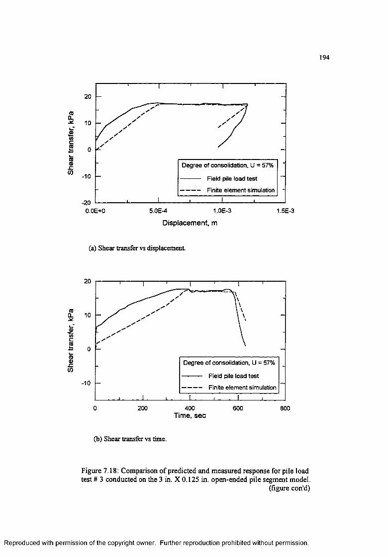
Shea
r tr
ansf
er,
kPa
Shea
r tr
ansf
er,
kPa
194
20
10
0
Degree of consolidation, U = 57%
-10 Field pile load test
Finite element simulation
-20 ----O.OE+O 1.0E-35.0E-4 1.5E-3
Displacement, m
(a) Shear transfer vs displacement
20
10
0
Degree of consolidation, U = 57%
Field pile load test
Finite element simulation-10
0 200 400 600 800Time, s e c
(b) Shear transfer vs time.
Figure 7.18: Comparison of predicted and measured response for pile load test # 3 conducted on the 3 in. X 0.125 in. open-ended pile segment model.
(figure con’d)
Reproduced with permission of the copyright owner. Further reproduction prohibited without permission.

Pore
w
ater
pre
ssur
e, k
Pa
Effe
ctiv
e ra
dial
str
ess,
kPa
195
100 -
50 -
Degree of consolidation, U = 57%
Field pile loasd test
Finite element simulation
200 400
Time, se c
600 800
(c) Effective radial stress vs time.
300
200 -
100200
Degree of consolidation, U = 57%
Field pile load test
Finite element simulation
I _ i_
400
Time, sec
600 800
(d) Pore water pressure vs time.
Reproduced with permission of the copyright owner. Further reproduction prohibited without permission.

Shea
r tr
ansf
er,
KPa
Shea
r tr
ansf
er,
kPa
196
30
20
10
0Degree of consolidation, U = 86%
Field pile load test
Finite element simulation-10
-20 ----O.OE+O 1.0E-35.0E-4 1.5E-3
Displacement, m
(a) Shear transfer vs displacement
30
20
10
0 Degree of consolidation, U = 86%
Field pile load test
Finite element simulation-10
0 150 300 450
Time, sec
(b) Shear transfer vs time
Figure 7.19: Comparison of predicted and measured response for pile load test # 4 conducted on the 3 in. X 0.125 in. open-ended pile segment model.
(figure con'd)
Reproduced with permission of the copyright owner. Further reproduction prohibited without permission.

Pore
w
ater
pre
ssur
e, k
Pa
Effe
ctiv
e ra
dial
str
ess,
kPa
197
250
200
150
100
50
00 150 300 450
Time, sec
(c) Effective radial stress vs time.
250
200
150
100
0 150 300 450
Time, sec
(d) Pore water pressure vs time.
Degree of consolidation, U = 86%
Field pile load test
Finite element simulation
i________I________■ ..
Degree of consolidation, U = 86%
Field pile load test
Finite element simulation
v___
Reproduced with permission of the copyright owner. Further reproduction prohibited without permission.

198
solution and the field measurements decrease as the excess pore water pressures dis
sipate. However, these differences did not affect the predictions of the shear transfer
during the simulation of the pile load tests.
Pile load test # 5 was simulated at 95% degree of consolidation. The test con
sisted of both loading and unloading cycles. Figure 7.20a shows the predicted and
measured variations of the shear transfer with the displacement. The numerical re
sults are lower than the field measurements. However, the behavior is well predicted
during the unloading-reloading cycles. Variations of the predicted and measured
shear transfer during the test are comparable, as shown in Figure 7.20b.
Figure 7.21a presents the variations of the estimated effective radial stress during
the test. Because of the leakage that occurred near the end of the experiment, the
measured total radial and pore water pressures were not considered for comparisons.
Therefore, only the finite element results are presented. The change in predicted
pore water pressure with time is shown in Figure 7.21b.
The numerical simulation of the final two-way cyclic pile load test was performed
near the end of consolidation. The test consisted of four tension-compression cycles.
The finite element results are in good agreement with the field measurements, as
presented in Figures 7.22 and 7.23.
The estimated shear transfer variations during the cycles axe slightly lower than
the measured values. However, the predicted and measured results are consistent,
and the numerical simulation accurately captured the response patterns during the
tension-compression cycles.
The predicted variations of effective radial stress and pore water pressure during
the test are shown in Figures 7.23a and 7.23b. The field measurements are not
presented due to their fluctuations during the test.
Reproduced with permission of the copyright owner. Further reproduction prohibited without permission.
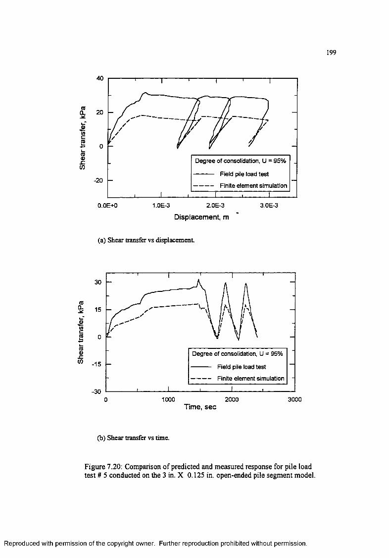
199
40
(0CL 20
l—<Dcnc2L_(00)r.CO
Degree of consolidation, U = 95%
Field pile load test
Finite element simulation-20
1.0E-3 2.0E-3 3.0E-3O.OE+O
Displacement, m
(a) Shear transfer vs displacement
CDQ.
inc(0k_
i—(0d)x:CO
Degree of consolidation, U = 95%
-15 Field pile load test
Finite element simulation
-301000 2000 30000
Time, s e c
(b) Shear transfer vs time.
Figure 7.20: Comparison of predicted and measured response for pile load test # 5 conducted on the 3 in. X 0.125 in. open-ended pile segment model.
Reproduced with permission of the copyright owner. Further reproduction prohibited without permission.

Pore
w
ater
pre
ssur
e, k
Pa
Effe
ctiv
e ra
dial
str
ess,
kPa
200
100
1000 2000o 3000
Time, se c
(a) Effective radial stress vs time.
300
100 1 1 1 1 1------------0 1000 2000 3000
Time, se c
(b) Pore water pressure vs time.
Figure 7.21: Predicted response during pile load test # 5 performed on the 3 in. X 0.125 in. open-ended pile segment model.
Reproduced with permission of the copyright owner. Further reproduction prohibited without permission.

Shea
r tr
ansf
er,
kPa
201
40
20
0
-20
Field pile load test
Finite element simulation-40
O.OOE+O 1.00E-3 2.00E-3-1.00E-3
Displacement, m
(a) Shear transfer vs displacement.
Figure 7.22: Comparison of predicted and measured response for the final cyclic pile load test conducted on the 3 in. X 0.125 in. open-ended pile segment model.
(figure con'd)
Reproduced with permission of the copyright owner. Further reproduction prohibited without permission.

Shea
r tr
ansf
er,
kPa202
40
20
0
-20
Field pile load test
Finite element simulation-40
0 1000 2000 3000 4000Time, sec
(b) Shear transfer vs time.
Reproduced with permission of the copyright owner. Further reproduction prohibited without permission.

Pore
w
ater
pre
ssur
e, k
Pa
Effe
ctiv
e ra
dial
str
ess,
kPa
203
100
75
50
2520000 1000 3000 4000
Time, sec
(a) Effective radial stress vs time.
250
200
150
1000 2000 3000 40000
Time, sec(b) Pore water pressure vs time.
Figure 7. 23: Predicted response for the final cyclic pile load test conducted on the 3 in. X 0.125 in. open-end pile segment model.
Reproduced with permission of the copyright owner. Further reproduction prohibited without permission.

204
7.5.2 The 3 in . x 0.065 in. O pen-ended P ile Segm ent M odel
Finite element simulation of the subsequent consolidation and pile load tests was
conducted to predict the response of the 3 in. x 0.065 in. open-ended pile segment
model. The estimated behavior of the model was compared with the results of the
field experiments. In order to avoid repetition, comparisons of the numerical results
with measurements are presented in Appendix B.
7.6 P ile Setup
Examination of Figures 7.16, 7.17, 7.18, 7.19, 7.20 and 7.22 indicates that the finite
element results are generally consistent with the field measurements. The predicted
variation of shear transfer during these tests is shown in Figure 7.24. The magnitude
of the estimated shear transfer at failure increased with the increase in the degree
of consolidation. The finite element successfully predicted the increase in the shaft
capacity with time (the pile setup).
The predicted and measured shear transfer values at failure are compared in
Figure 7.25. The comparison includes the peak and residual shear transfer values.
Within the estimated and measured values, the difference between the peak and the
residual is small. Finite element solutions axe consistent with the measured increase
with time in the peak and residual shear transfer values. At the end of consolidation,
the predictions axe slightly lower than the field measurements.
The response of the open-ended pile during pile driving, subsequent consolida
tion, and pile load tests was predicted using numerical and finite element methods.
The numerical solutions for the different life stages of the open-ended pile axe suc
cessfully achieved. These solutions are found to be consistent with the field measure
ments.
Reproduced with permission of the copyright owner. Further reproduction prohibited without permission.

Reproduced
with perm
ission of the
copyright ow
ner. Further
reproduction prohibited
without
permission.
20
15
10U = 95%
U = 86%
U = 57%5
U = 36%
U = 16%
0 It—0.0E+0 5.0E-4 1.0E-3 1.5E-3 2.0E-3
Displacement, m
Figure 7.24: The finite element prediction of the increase in shear transfer for pile load tests conducted during soil consolidation around the 3 in. X 0.125 in. pile segment model.
toO
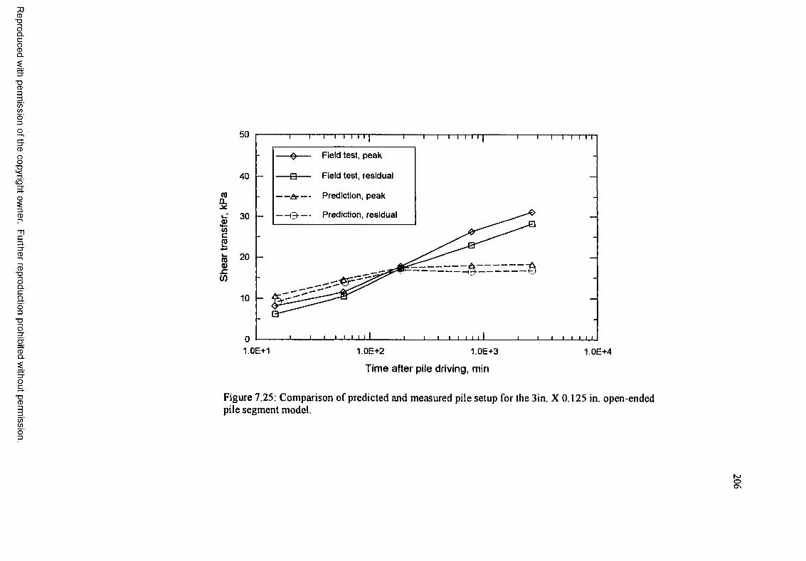
Reproduced
with perm
ission of the
copyright ow
ner. Further
reproduction prohibited
without
permission.
(0CLyc.uT£.<nc2i .(0Q)x z(/)
50
Field test, peak
Field test, residual40
— A- — - Prediction, peak
— Q- — - Prediction, residual30
20
10
0 ---1.0E+1 1.0E+2 1.0E+3 1.0E+4
Time after pile driving, min
Figure 7.25: Comparison of predicted and measured pile setup for the 3in. X 0.125 in. open-ended pile segment model.
NJOO N

CHAPTER 8 NUMERICAL EXPERIMENTS ON A FULL-SCALE CLOSED-ENDED PILE
8.1 Introduction
Numerical simulations of the behavior of closed-ended as well as open-ended pile
segment models during driving, consolidation, and load testing were successfully
conducted. The numerical study was performed on pile segment models due to
the availability of the field experiments necessary for the verification and evaluation
schemes. However, the method is also applicable for investigating the behavior of
full-scale friction piles driven into saturated clay. For demonstration, finite element
numerical simulation of the behavior of a full scale pile was earned out.
This chapter presents the results of the numerical simulation of the various life
stages of a full-scale friction pile driven into saturated clay.
8.2 Pile Characteristics
A full-scale pile, 0.5 m in diameter and 10 m in length, was considered in order to
perform various numerical experiments. The material parameters, soil conditions,
and numerical stability and convergence parameters of Sabine clay were used in the
simulation.
The soil mass was discretized according to the finite element mesh presented
in Figure 8.1. The mesh consists of 377 elements and 1216 nodes. The 8-node
axisymmetric solid element CAX8RP was used to form the finite element mesh. The
soil mass around the pile was modeled as the HiSS- material.
207
Reproduced with permission of the copyright owner. Further reproduction prohibited without permission.

k5 m 208
Element 8-node ABAQUS-CAX8RP 377 elements 1216 nodes
Figure 8.1: The finite element mesh used to discretize the soil around the pile.
R eproduced with perm ission of the copyright owner. Further reproduction prohibited without perm ission.

209
8.3 Simulation o f Pile Driving
The pile was driven at the ground surface. As a result, the soil mass around the pile
was assumed to be affected by pile driving. The simple pile approach (Baligh, 1984),
developed for deep penetration of closed-ended piles, was utilized to simulate pile
driving.
At the end of driving, the effective stresses of the soil around the pile significantly
decreased. In contrast, the effective stresses of the soil in the far field remained under
AT,,-conditions. Figure 8.2 shows that low magnitudes of predicted effective stresses
around the pile extend to about ten times pile diameter. The effective radial stress
decreased from about 50 kPa before driving to 12 kPa immediately after driving.
The predicted pore water pressure distribution at the end of pile driving is de
picted in Figure 8.3. Immediately after pile driving, excess pore pressure developed
in the soil around the pile, up to a distance of about ten times pile diameter.
8.4 Consolidation and Pile Load Tests
The initial conditions required for the finite element simulation of consolidation were
obtained at the end of driving. They include stresses and pore water pressures
that satisfy equilibrium, strain compatibility, and constitutive relations. The finite
element simulation was conducted based on the nonlinear transient analysis available
in ABAQUS.
The effective stresses gradually increased as the excess pore water pressures dis
sipated during consolidation. Dissipation of the excess pore water pressure during
soil consolidation around the pile is presented in Figure 8.4. Most of the excess pore
water pressures dissipated within 1000 hours after driving. Konard and Roy (1987)
reported that the excess pore water pressures generated during driving 22 cm di
ameter steel piles were dissipated 600 hours after driving. For the 0.5 diameter pile
R eproduced with perm ission of the copyright owner. Further reproduction prohibited without perm ission.
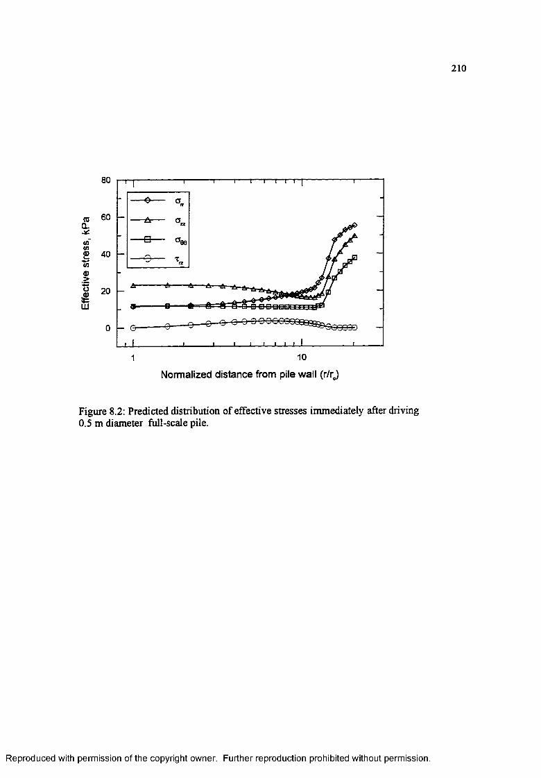
Effe
ctiv
e st
ress
, kP
a
210
80
60
40
20
0
Figure 8.2: Predicted distribution of effective stresses immediately after driving 0.5 m diameter full-scale pile.
□ O O D D I
o o o c o
1 10
Normalized distance from pile wall (r/r)
R eproduced with perm ission of the copyright owner. Further reproduction prohibited without perm ission.

Pore
w
ater
pre
ssur
e, k
Pa211
120
100
80
60101
Normalized distance from pile wall (r/rj
Figure 8.3: Predicted distribution of pore water pressure immediately after driving 0.5 m diameter full-scale pile.
Reproduced with permission of the copyright owner. Further reproduction prohibited without permission.

Reproduced
with perm
ission of the
copyright ow
ner. Further
reproduction prohibited
without
permission.
140 1 1—i—i i n~ 1 ----------- 1-------- 1— i— i i i i
(0CL 120
S3 w tn 9>
<oCD$a>L -oQ.
100
80
60 1.0E+0
_i i i i i i 11 j i i i i i 111 j i i i 1111 j i i i i 111 1
1.0E+1 1.0E+2 1.0E+3
Time after pile driving, hours
1.0E+4
Figure 8.4: Variation with time of predicted pore water pressure during soil consolidation around the 0.5 m diameter full-scale pile.
212

213
simulated herein, it is therefore acceptable for most of the excess pore water pres
sures to dissipate during the 1000 hours. Furthermore, the pattern of the dissipation
curve is similar to those obtained in the field by the Earth Technology Corp. (1986).
The estimated increase in the effective radial stress during consolidation is de
picted in Figure 8.5. At the end of consolidation, the maximum increase in the
effective stresses developed with complete dissipation of the excess pore water pres
sures. The effective radial stress increased from 12 kPa immediately after driving to
53 kPa at the end of consolidation.
Four static compression load tests were simulated during the consolidation phase.
These tests were simulated at 10, 43, 78, and 100 percent degrees of consolidation.
For each pile load test, linear displacement was applied during the test until the
shear transfer at the soil-pile interface became constant with time. Variations of
shear transfer with displacement for these tests Me presented in Figure 8 .6 . The
predictions of shear transfer change with displacement axe consistent with those
obtained in the previous chapters.
8.5 P ile Setup
Simulating pile load tests at different time intervals during consolidation provided the
necessary means to estimate pile setup. During the pile load test, the maximum shear
stress at the soil-pile interface represents the maximum mobilized skin friction for
resisting pile loading. For these simulated tests, the variations with displacement of
the average skin friction along the pile shaft Me shown in Figure 8 .6 . The maximum
average value for each pile load test was identified (Figure 8 .6 ). Shown in Figure
8.7 is the variation with time of the average skin friction along the pile shaft for
these load tests. Examination of Figure 8.7 indicates that the bearing capacity of
the pile increased during soil consolidation and a pile setup developed. The average
Reproduced with permission of the copyright owner. Further reproduction prohibited without permission.
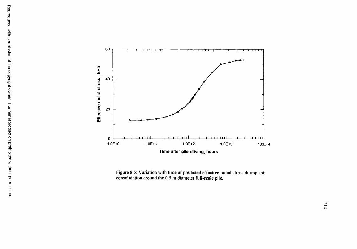
Reproduced
with perm
ission of the
copyright ow
ner. Further
reproduction prohibited
without
permission.
60 i --------- 1— i— i i i i i i ----- 1— i—i i i i i ~ i-------1— i—i~i i n
coQ.
g 40
.£<nraTJroa)>
sSLLl
20
_i i i i i i 11 J i i i i i 111 i i i i i i n J I 1- 1 L l l l l
1.0E+0 1.0E+1 1.0E+2 1.0E+3
Time after pile driving, hours
1.0E+4
Figure 8.5; Variation with time of predicted effective radial stress during soil consolidation around the 0.5 m diameter full-scale pile.
N>£

Reproduced
with perm
ission of the
copyright ow
ner. Further
reproduction prohibited
without
permission.
(0CL
i t fros zV)a>£o>co(0co
* 3oEc12<na>a)2a>><
10
5
Degree of consolidation
U = 100%
U = 78%
U = 43%0U = 10%
0E+0 2E-3 4E-3 6E-3
Displacement, m
Figure 8.6: Variations with displacement of average skin friction along the shaft for different pile load tests conducted during soil consolidation around the 0.5 m diameter full-scale pile.
NJ •—*

Ave
rage
sk
in fri
cition
alo
ng
the
shaf
t, kP
a
216
10
8
6
4 -----1.0E+0 1.0E+1 1.0E+2 1.0E+3 1.0E+4
Time after pile driving, hour
Figure 8.7: Predicted increase in average skin friction along the shaft of the pile during soil consolidation around the 0.5 diameter full-scale pile.
Reproduced with permission of the copyright owner. Further reproduction prohibited without permission.

217
skin, friction increased from about 5 kPa six hours after driving to about 7.8 kPa at
the end of consolidation.
Reproduced with permission of the copyright owner. Further reproduction prohibited without permission.

CHAPTER 9 SUMMARY, CONCLUSIONS, AND
RECOMMENDATIONS
9.1 Summary
In this study, a general method for predicting pile setup, or the increase in bearing
capacity of friction piles driven into saturated clay, was developed based on consis
tent formulations during pile driving, consolidation, and loading. The behavior of
friction piles driven into saturated clay was investigated during pile driving, sub
sequent consolidation, and load testing. During soil consolidation, the response of
the pile upon loading provided the quantitative estimate of the variation of the pile
bearing capacity over time. The method was applied to both partial-displacement
(open-ended) and full-displacement (closed-ended) piles.
An HiSS constitutive interface model named was developed in order to capture
soil behavior under severe shear deformation at the soil-pile interface. The model
could also be used to characterize the behavior of the soil in the far field. The
developed model was implemented into the ‘strain to stress’ algorithm as well as into
the finite element program ABAQUS, in which the theory of nonlinear porous media
is used to perform the analysis.
The strain path method was used to simulate pile driving. The simple pile ap
proach was utilized for full-displacement (closed-ended) piles, while the concept of
the ‘ideal’ open-ended pile was utilized for partial-displacement (open-ended) piles.
A computer code was developed to obtain the strain field in the surrounding soil re
sulting from pile driving. This code used the proposed interface model to predict
the stress field in the soil around the pile during driving. Numerical simulations of
pile driving were performed in order to predict the field behavior of well-documented
218
Reproduced with permission of the copyright owner. Further reproduction prohibited without permission.

219
field experiments conducted on pile segment models at Sabine Pass in Texas. Simu
lations included closed-ended as well as open-ended piles.
The finite element simulation of soil consolidation around the pile was conducted.
During the consolidation phase, pile load tests were simulated at different time inter
vals. The purpose of simulating these tests was to predict the variation of pile bear
ing capacity with time. These simulations were conducted using full-displacement
(closed-ended) as well as partial-displacement (open-ended) pile segment models.
The results of the finite element analysis were evaluated by comparing them with
pile behavior measurements in the field.
In this study, numerical simulations were performed on pile segment models due
to the availability of the field experimental tests necessary for the verification and
evaluation schemes. However, the method was also used to investigate the behavior
of full-scale friction piles driven into saturated clay. Finite element numerical exper
iments were conducted using a full-scale friction pile driven into saturated clay. The
numerical simulation included the various life stages of a full-scale driven friction
pile (pile driving, subsequent consolidation, and load testing). The variation of pile
bearing capacity with time was also investigated.
9.2 Conclusions
The following general conclusions are derived from this study:
• The ability of the general method developed for predicting the pile setup of
friction piles driven into saturated clay was demonstrated. The finite element
results were verified with respect to field experiments conducted on pile segment
models.
• Successful predictions of pile setup for both partial-displacement and full-
displacement pile segment models were achieved.
Reproduced with permission of the copyright owner. Further reproduction prohibited without permission.

220
• Numerical experiments showed that the method is applicable for the prediction
of the pile setup of full-scale piles.
• Investigating the behavior of the pile during its various life stages resulted in
the reasonable evaluation of the pile bearing capacity.
• Finite element simulations of different pile load tests during soil consolidation
provided quantitative measures for the variation of pile bearing capacity over
time.
• An HiSS interface model named model was developed and evaluated with
respect to field experiments. This model was successfully used to predict soil
behavior under severe shearing at the soil-pile interface.
9.3 Recom m endations
The following are some recommendations for future research:
• Incorporating the effect of thixotropy on the pile setup.
• Further research to modfiy the constitutive model and to consider the changes
in the soil fabric during a loading (consideration of the micromechanical be
havior in the constitutive model).
• Studying the pile setup for a pile group.
• Investigating the effect of soil-plug response on the behavior of open-ended
piles and on the setup.
• Pefroming numerical experiments on full-scale piles with different dimensions
and considering different soil conditions. This can initiate a pile setup design
charts.
Reproduced with permission of the copyright owner. Further reproduction prohibited without permission.

221
• Conducting an experimental program to obtain stresses and pore water pres
sures in the soil during pile driving, subsequent consolidation, and loading.
These measurements will provide the necessary means to evaluate the predic
tions of the stresses and pore water pressures away from the pile.
Reproduced with permission of the copyright owner. Further reproduction prohibited without permission.

R E F E R E N C E S
• ABAQUS/Standard (1995). Hibbitt, Karlsson & Sorensen, Inc.
• Abramowitz, M., and Stegnn, I. A. (1965). “Handbook of Mathematical Functions,” Dover Publications, New York.
• Acar, Y. B., and Tumay, M. T. (1986). “Strain Field Around Cones in Steady Penetration,” Journal of Geotechnical Engineering, ASCE, Vol. 112, No. GT2, p p 207-213.
• Ahmad, I. (1990). “Investigation of Normalized Behavior of Resedimented Boston Blue Clay Using the Geonor Direct Simple Shear Apparatus,” MS Thesis, MIT, Cambridge, Massachusetts.
• Azzouz, A. S. (1986). “Role of Load Tests in Friction Pile Design,” Journal of Geotechnical Engineering, ASCE, Vol. 112, No. GT4, pp 407-423.
• Azzouz, A. S., and Baligh, M. M. (1984). “Behavior of Friction Piles in Plastic Empire Clays,” MIT Research Report, MA.
• Azzouz, A. S., Baligh, M. M., and W hittle, A. J. (1990). “Shaft Resistance of Pile in Clay,” Journal of Geotechnical Engineering, ASCE, Vol. 116, No. GT2, pp 205-221.
• Azzouz, A. S., and Lutz, D. G. (1986). “Shaft Behavior of a Model Pile in Plastic Empire Clay,” Journal of Geotechnical Engineering, ASCE, Vol. 112, No. GT4, pp 389-406.
• Azzouz, A. S., and Morrison, M. J. (1988). “Field Measurements on Model Pile in Two Clay Deposits,” Journal of Geotechnical Engineering, Vol. 114, No. 1, pp 104-121.
• Baligh, M. M. (1975). “Theory of Deep Site Static Cone Penetration Resistance,” Research Report No. R75-56, Department of Civil Engineering, MIT, Cambridge, Massachusetts, 133 Pages.
• Baligh, M. M. (1984). “Simple Pile Approach to Pile Installation in Clays,” Analysis and Design of Pile Foundations, J. R. Meyer, (Editor), pp 310-330.
• Baligh, M. M. (1985). “Strain Path Method,” Journal of Geotechnical Engineering, ASCE, Vol. I l l , No. GT7, pp 1108-1196.
• Baligh, M. M. (1986a). “Undrained Deep Penetration, I: Shear Stresses,” Geotechnique, Vol. 36, No. 4, pp 471-485.
• Baligh, M. M. (1986b). “Undrained Deep Penetration, II: Pore Pressures,” Geotechnique, Vol. 36, No. 4, pp 487-501.
222
Reproduced with permission of the copyright owner. Further reproduction prohibited without permission.

223
• Baligh, M. M., Azzouz, A. S. and Chin, C. T. (1987). “Disturbance due to Ideal Tube Sampling,” Journal of Geotechnical Engineering, ASCE, Vol. 113, No. GT7, pp 793-757.
• Baligh, M. M., and Levadoux N., J. (1980). “Pore Pressure Dissipation After Cone Penetration,” Report No. MITSG 80-13, MIT, Cambridge, Massachusetts.
• Banerjee, P. K., Davies, T. G., and Fathallah, R. C. (1982). “Behavior of Axially Loaded Driven Piles in Saturated Clay from Model Studies,” Chapter 5 in Developments in Soil Mechanics and Foundation Engineering, Edited by P. K. Banerjee, Applied Science Publishers Ltd., England.
• Banerjee, P. K., and Fathallah, R. C. (1979). “Stresses and Pore Water Pressures Around a Continuously Penetrating Pile,” Civil Engineering Department, University College, Cardiff.
• Banerjee, P. K., and Yousif, N. B. (1986). “A Plasticity Model for the Mechanical Behavior of Anisotropically Consolidated Clays,” Int. J. Num. Analyt. Meth. Geomechanics, Vol. 10, pp 521-541.
• Bartolomy, A. A. and Yushkov, B. S. (1985). “Variation in Time of Capacity of Pile Foundations in Clay,” P roc .llth Int. Conf. of Soil Mech. and Found. Eng., San Francisco, pp 1517-1520.
• Beringen, F. L., and De Ruiter, J. (1987). “Pile Foundation for Offshore Fixed Platforms,” in B. K. Mazurkiewicz, (ed.), Offshore Platforms and Pipelines: Selected Contributions, Series on Rock and Soil Mechanics, Vol. 13, pp 165— 216.
• Bjerrum, L., Brinch Hansen, J., and Sevaldson, R. (1958). “Geotechnical Investigation for a Quay Structure in Horten,” NGI, No. 28, 1-17.
• Blessey, W.E., and Lee, P.Y. (1980). “Report on Wave Equation Analysis of Pile Driving in the New Orleans Area,” Pile Driving Contractors Association of New Orleans Inc.
• Bogard, J . D., and Matlock, H. (1979). “A Model Study of Axially Loaded Pile Segments, Including Pore Pressure Measurements,” Report to the American Petroleum Institute, Austin, Texas.
• Bogard, J . D., and Matlock, H. (1990a). “In-Situ Pile Segment Model Experiments at Empire, Louisiana,” Proceedings, Offshore Technology Conference, Paper 6323, Houston, Texas, USA.
• Bogard, J. D., and Matlock, H. (1990b). “In-Situ Pile Segment Model Experiments at Harvey, Louisiana,” Proceedings, Offshore Technology Conference, Paper 6324, Houston, Texas, USA.
Reproduced with permission of the copyright owner. Further reproduction prohibited without permission.

2 2 4
• Bogard, J. D., and Matlock, H. (1990c). “Application to Model Pile Tests to Axial Pile Design,” Proceedings, Offshore Technology Conference, Paper 6376, Houston, Texas, USA.
• Bond, A. J., and Jardine, R. J. (1991). “Effects of Installing Displacement Piles in a High OCR Clay,” Geotechnique, Vol. 41, No. 3, pp 341-363.
• Bozozuk, M., Fellenius, B. H., and Samson, L. (1978). “Soil Disturbance from Pile Driving in Sensitive Clay,” Canadian Geotechnical Journal, Vol 15, pp 346-361.
• Burland, J. (1973). “Shaft Friction of Piles in Clay a Simple Fundamental Approach,” Proc., Ground Engineering, 6(3), pp 48-51.
• Butterfield, R., and Banerjee, P. K. (1970). “The Effect of Pore Water Pressures on the Ultimate Bearing Capacity of Driven Piles,” Proc. of the 2nd Southeast Asian Conference on Soil Engineering, Singapore, pp 385-394.
• Carter, J. P., Randolph, M. F., and Wroth, C. P. (1979). “Stress and Pore Pressure Changes in Clay During and After the Expansion of the of a Cylindrical Cavity,” International Journal for Numerical and Analytical Methods in Geomechanics, Vol. 3, pp 305-322.
• Chandler, R. J. (1968). “The Shaft Friction of Piles in Cohesive Soils in Terms of Effective Stresses,” Civil Engineering and Public Works Review, 63, pp 48- 51.
• Chandler, R. J., and Martins, J. P., (1982). “An Experimental Study of Skin Friction Around Piles in Clay,” Geotechnique, Vol. 32, No. 2, pp 119-132.
• Chen, Z., and Schreyer, H. L. (1987). “Simulation of Soil-Concrete Interface with Nonlocal Constitutive Models,” Journal of Engineering Mechanics, ASCE, Vol. 113, No. 11, pp 1665-1677.
• Chin, C. T. and Baligh, M. M. (1983). “Deformations and Strains due to Open-Ended Pile Installation in Saturated Clay,” Reseaxch Report No. R83- 17, Dept, of Civil Eng., MIT, Cambridge, MA 02139.
• Chopra, M. B., and Dargush, G. F. (1992). “Finite-Element Analysis of Time- Dependent Large-Deformation Problems,” International Journal for Numerical and Analytical Methods in Geomechanics, Vol. 16, pp 101-130.
• Chow, Y. K., Karunaratne, G. P., Wong, K. Y., and Lee, S. L. (1988). “Prediction of Load Carrying Capacity of Driven Piles,” Canadian Geotechnical Journal, Vol. 25, pp 13-25.
• Chung, K. Y. C. (1988). “Excess Pore Pressure Induced by Pile Driving in Sensitive River Sediment” Proceedings, 3rd. Int. Seminar on the Application of Stress-Wave Theory to Piles,” Ottawa, B. H. Fellenius, Ed., pp 679-688.
Reproduced with permission of the copyright owner. Further reproduction prohibited without permission.

225
• Clark, J . I., and Meyerhof, G. G. (1972). “The Behavior of Piles Driven in Clay. I. An Investigation of Soil Stress and Pore Water Pressure as Related to Soil Properties,” Canadian Geotechnical Journal, Vol. 9, pp 351-373.
• Clark, J. I., and Meyerhof, G. G. (1973). “The Behavior of Piles Driven in Clay. II. Investigation of the Bearing Capacity Using Total and Effective Strength Parameters,” Canadian Geotechnical Journal, Vol. 10, pp 86—102.
• Cooke, R. W., and Price, G. (1973). “Strains and Displacements Around Friction Piles,” Proceedings, 8th ICSMFE, Moscow, Vol. 2, No. 1 , pp 53-60.
• Coop, M. R., and Wroth, C. P. (1989). “Field Studies of an Instrumented Model Pile in Clay,” Geotechnique, Vol. 39, No. 4, pp 679-696.
• Cox, W. R., and Kraft, L. M. (1979). “Axial Load Tests on 14-inch Pipe Piles in Clay,” Proceedings, Offshore Technology Conference, Paper 3491, Houston, Texas, USA.
• Cummings, A. E., Kerkhoff, G. 0 ., and Peck, R. B. (1950). “Effect of pile Driving in Soft Clay,” Trans. ASCE, vol. 115, 275-286.
• Dafalias, Y. F., and Herrmann, L. R. (1986). “Bounding Surface Plasticity II: Application to Isotropic Cohesive Soils,” J. Eng. Mech., ASCE, Vol. 112, No.12, pp 1263-1291.
• D’Appolonia, D. J. and Lambe, T. W. (1971). “Performance of Four Foundation on End-Bearing Piles,” JSMFD, ASCE, 97(10), 1359-1377.
• de Mello, V. F. B. (1969). “Foundations of Buildings on Clay,” S tate-of-the- Art Report, Proc. 7th ICSMFE, 49-136.
• Desai, C. S. (1978). “Effects of Driving and Subsequent Consolidation on Behavior of Driven Piles,” Int. Journal of Numerical and Analytical Methods in Geomechanics, Vol. 2, pp 283-301.
• Desai, C. S. (1980). “A General Basis for Yield, Failure and Potential Functions in Plasticity,” Int. J. Num. Analyt. Meth. in Geomechanics, Vol. 4, pp 361— 375.
• Desai, C. S., Galagoda, H. M., and Wathugala, G. W. (1987). “Hierarchical Modelling for Geologic Materials and Discontinuities-Joints, Interfaces,” Invited Paper, Proceedings of the Second Int. Conf. on Constitutive Laws for Engineering Materials: Theory and Applications, Tucson, Arizona, Desai et al (Eds.), Elsevier, New York, Vol. 1, pp 81-95.
• Desai, C. S., Sharma, K. G., Wathugala, G. W., and Rigby, D. B. (1991) “Implementation of Hierarchical Single Surface and Models in Finite Element Procedures,” International Journal of Analytical and Numerical Methods in Geomechanics, Vol. 15, pp 649-680.
Reproduced with permission of the copyright owner. Further reproduction prohibited without permission.

226
• Desai, C. S., Somasundaram, S., and Frantziskonis, G. N. (1986). “A Hierarchical Approach for Constitutive Modelling of Geologic Materials,” Int. J. Num. Analyt. Meth. Geomechanics, Vol. 10, pp 225-257.
• Desai, C. S., and Wathugala, G. W. (1987) “Hierarchical and Unified Models for Solids and Discontinuities (Joints/Interfaces),” Short Course Notes, Second Int. Conf. on Constitutive Laws for Engineering Materials: Theory and Applications, Tucson, Arizona, pp 31-124.
• Desai, C. S., Wathugala, G. W., and Matlock, H. (1993). “Constitutive Model for Cyclic Behavior of Clays. I: Applications,” Journal of Geotechnical Engineering, ASCE, Vol. 119, No. GT4, pp 730—748.
• Desai, C. S., Wathugala, G. W., and Navayogarajah, N. (1989). “Developments in Hierarchical Modelling for Solids and Discontinuities and Applications,” Invited Paper, Proc. International Conference on Constitutive Laws for Engineering Materials, Chongqing, China, International Academic Publishers, Pregamon Press, Vol. 1, pp 43-53.
• Desai, C. S., Wathugala, G. W., Sharma, S. K., and Woo, L. (1990). “Factors Affecting Reliability of Computer Solutions with Hierarchical Single Surface Models,” International Journal of Computer Methods in Applied Mechanics and Engineering, Vol. 82, pp 115-137.
• DiMaggio, F. L., and Sandler, I. S. (1971). “Material Model for Granular Soils,” Journal of the Engineering Mechanics Division, ASCE, Vol. 97, No. EM3, pp 935-950.
• Earth Technology Corporation (1986). “Pile Segment Tests - Sabine Pass : Some Aspects of the Fundamental Behavior of Axially Loaded Piles in Clay Soils,” ETC Report No. 85-007, Houston, Texas.
• Eide, 0 ., Hutchinson, J. N., and Landva, A. (1961). “Short and Long-Term Test Loading of A Friction Pile in Clay,” Proc. 5th Int. Conf. of Soil Mech. and Found. Eng., pp 45-54, Paris.
• Esrig, M. I., Kirby, R. C., Bea, R. G., and Murphy, B. S. (1977). Initial Development of A General Effective Stress Method for the Prediction of Axial Capacity of piles in Clay,” Proceedings, Offshore Technology Conference, Houston, Texas, USA.
• Flaate, K. (1968). “The Bearing Capacity of Friction Piles in Clay (in Norwegian),” Norw. Road Res. Lab., Oslo, 38 p.
• Flaate, K. (1972). “Effects of Pile Driving on Clays,” Canadian Geotechnical Journal, Vol. 9, pp 81-88.
Reproduced with permission of the copyright owner. Further reproduction prohibited without permission.

2 27
• Flaate, K., and Seines P. (1977). “Side Friction of Piles in Clay,” Proc. 9th Int. Conf. on Soil Mechanics and Foundation Engineering, Tokyo, Japan, Vol. 1, pp 517-522.
• Fellenius, B. H., Riker, R. E., O’Brien, J. A., and Tracy, G. R. (1989). “Dynamic and Static Testing in Soils Exhibiting Set-Up,” Journal of Geotechnical Engineering, ASCE, Vol. 115, No. GT7, pp 984-1001.
• Fellenius, B. H., and Samson, L. (1976). “Testing of Drivability of Concrete Piles and Disturbance to Sensitive Clay,” Canadian Geotechnical Journal, Vol 13, pp 139-160.
• Galagoda, M. H. (1986). “Nonlinear Analysis of Soil Porous Media and Applications,” Ph.D. Dissertation, University of Arizona, Tucson, USA.
• Goble, G. G., Rausche, F., and Likins, G. E. (1980). “The analysis of Pile Driving A State-of-the-A rt,” Proceedings, 1st. Int. Seminar on the Application of Stress-Wave Theory on Piles,” Stockholm, H. Bredenberg, Ed., A. A. Balkema, Rotterdam, pp 131-162.
• Grosch, J. J., and Reese, L. C. (1980). “Field Tests of Small-Scale Pile Segments in a Soft Clay Deposit Under Repeated Axial Loading,” Proceedings, Offshore Technology Conference, Paper 3869, Houston, Texas, USA.
• Heydinger A. G., and O’Niell, M. W. (1986). “Analysis of Axial Pile-Soil Interaction in Clay,” International Journal for Numerical and Analytical Methods in Geomechanics, Vol. 10, pp 367-381.
• Housel, W. S., and Burkey, J. R. (1948). “Investigation to Determine the Driving Characteristics of Piles in Soft Clay,” Proc. 2nd ICSMFE, Vol. 5, 146-154.
• Ismael, N. F., and Klym, T. W. (1979). “Pore Water Pressures Induced by Pile Driving,” Journal of the Geotechnical Engineering Division, ASCE, Vol. 105, No. GT11, pp 1349-1354.
• Jaime, A., Romo, M. P., and Resendiz, D. (1990). “Behavior of Friction Piles in Mexico City Clay,” Journal of Geotechnical Engineering, ASCE, Vol. 116, No. GT6 , pp 915-931.
• Jardine, R. J., and Bond, A. J. (1989). “Behavior of Displacement Piles in a Heavily Overconsolidated Clay,” Proceedings of the 12th International Conference on Soil Mechanics and Foundation Engineering, Rio de Janeiro, Vol. 2, pp 1147-1151.
• Katti, D. R. (1991). “Constitutive Modelling and Testing of Saturated Marine Clay,” Ph.D. Dissertation, Department of Civil Engineering, University of Arizona, Tucson, Arizona.
Reproduced with permission of the copyright owner. Further reproduction prohibited without permission.

228
• Kiousis, P. D. (1985). “Large Strain Theory as Applied to Penetration Mechanisms in Soils,” Ph.D. Dissertation, Department of Civil Engineering, Louisiana State University, Baton Rouge, LA.
• Kiousis, P. D., Voyiadjis, G. Z., and Tumay, M. T. (1988). “A Large Strain Theory and Its Application in the Analysis of the Cone Penetration Mechanism,” International Journal for Numerical and Analytical Methods in Geomechanics, Vol. 12, pp 45-60.
• Kirby, R.C., and Wroth, C. P. (1977). “Applications of Critical State Soil Mechanics to the Prediction of Axial Capacity for Driven Piles in Clay,” Offshore Technology Conference, Houston, Texas, Paper No. 2942.
• Koizumi, Y., and Ito, K. (1967). “Field Tests with Regard to Pile Driving and Bearing Capacity of Piled Foundation,” Soil and Found., VII (3), pp 30-53.
• Konard, J. M. and Roy, M. (1987). “Bearing Capacity of Friction Piles in Marine Clay,” Geotechnique, Vol. 37, No. 2, pp 163-175.
• Kraft, L. M., Cox, W. R., and Vemer, E. A. (1980). “Pile Load Tests: Cyclic Loads and Varying Load Rates,” Journal of the Geotechnical Engineering Division, ASCE, Vol. 107, No. G Tl, pp 1-19.
• Kraft, L. M., Focht, J . A., and Amerasinghe, S. F. (1981). “Friction Capacity of Piles Driven into Clay,” Journal of the Geotechnical Engineering Division, ASCE, Vol. 107, No. G T ll, pp 1521-1541.
• Kuchemann, D., and Weber, J. (1953). “Aerodynamics of Propulsion,” McGraw- Hill, New York, 1953.
• Ladanyi, B. (1963). “Expansion of a Cavity is Saturated Medium,” JSMFD, ASCE, Vol. 89, SM4, pp 127-161.
• LADODT (1994), Personal Communications.
• Lambe, T. W., and Horn, H. M. (1965). “The Influence on an Adjacent Building of Pile Driving for the M.I.T. Materials Center,” Proceedings, 6th ICSMFE, Montreal, Vol. II, pp 280-284.
• Leong, C. E., and Randolph, M. F. (1991). “Finite Element Analyses of Soil Plug Response,” International Journal for Numerical and Analytical Methods in Geomechanics, Vol. 15, pp 121-141.
• Leung, C. F., Radhakrishnan, R., and Tan, S. (1991) “Performance of Precast Driven Piles in Marine Clay,” Journal of Geotechnical Engineering, ASCE, Vol. 117, No. 4, pp 637-657.
Reproduced with permission of the copyright owner. Further reproduction prohibited without permission.

229
• Levadoux, J. N., and Baligh, M. M. (1980). “Pore Pressures During Cone Penetration in Clays,” Report No. MITSG 80-12, Dept, of Civil Eng., MIT, Cambridge, MA.
• Lo, K. Y., and Stermac, A. G. (1965). “Induced Pore Pressures During Pile Driving Operations,” Proc. 6th ICSMFE, vol. 2, 285.
• Matlock, H., and Bogard, J. D. (1973). “Lateral Load Behavior of Piles and Pile Groups Under Surcharge,” Report to Chevron Oil Filed Research Company, Austin, Texas.
• Matlock, H., and Bogard, J. D. (1975). “Pile Model Scale Effects and Cyclic Vane Shear Tests,” Report to Chevron Oil Filed Research Company, Austin, Texas.
• Matlock, H., and Holmquist, D. V. (1976). “A Model Study of Axially Loaded Piles in Soft Clay,” Report to the American Petroleum Institute, Austin, Texas.
• Matlock, H., and Tucker, R. L. (1961). “Lateral-Load Tests of an Instrumented Pile at Sabine, Texas,” Report to Shell Oil Company on Research Conducted by Engineering Science Consultants, Austin, Texas.
• McCammon, N. R., and Golder, H. Q. (1970). “Some Loading Tests on Long Pipe Piles,” Geotechnique, Vol. 20, No. 2, pp 171-184.
• McClleland Engineers (1969). “ Additional Soil Investigation, Pile Research Program, Block 100, Eugene Island Area,” Report to Shell Oil Company.
• McClleland, B. (1972). “Design and Performance of Deep Foundations in Clay,” General Report ASCE Specialty Conf. Performance of Earth and Earth Supported Structures, 2, pp 111-114.
• McManis, K. L., Folse, M. D., and Elias, J. S. (1988). “Determining Pile Bearing Capacity by Some Means Other than the Engineering News Formula,” Research Report No. 234, LTRC, Baton Rouge, LA.
• Meyerhof, G. G. (1976). “Bearing Capacity and Settlement of Pile Foundations,” Journal of Geotechnical Engineering Division, ASCE, Vol. 102, No. 3, pp 197-228.
• Milne-Thompson, L. M. (1976). “Theoretical Hydrodynamics,” 5th Ed., Revised, The Mac Millan Press, London, England.
• Mitchell, J. K. (1960). “Fundamental Aspects of Thixotropy in Soils,” JSMFD, ASCE, Vol. 86, No. SM3, pp 19-52.
• Mitchell, J. K. (1993). “Fundamentals of Soil Behavior,” John Wiley and Sons, New York, 437 pp
Reproduced with permission of the copyright owner. Further reproduction prohibited without permission.

230
• Nishida, Y. (1964). “A Basic Calculation on the Failure Zone and the Initial Pore Pressure Around a Driven Pile,” Proc. of the First Reg. Asian Conf. on Soil Mech. and Found. Eng., Tokyo, 1 , pp 217-219.
• Orrje, O., and Broms, B. (1967). “Effects of Pile Driving on Soil Properties,” Journal of the Soil Mechanics and Foundation Division, ASCE, Vol. 93, No. SM5, pp 59-73.
• Parry, R. H. G., and Swain, C. W. (1977). “Effective Stress M ethod of Calculating Skin Friction on Driven Piles in Soft Clay,” Ground Engineering 10, No. 3, pp 24-26.
• Peck, R. B. (1958). “A Study of the Comparative Behavior of Friction Piles,” Special Report 36, Highway Research Board.
• Poulos, H. G., and Davis, E. H. (1980). “Pile Foundation Analysis and Design,” John Wiley and Sons Inc.
• Randolph, M. F., Carter, J. P., and Wroth, C. P. (1979). “Driven Piles in Clay-the Effects of Installation and Subsequent Consolidation,” Geotechnique, Vol. 29, No. 4, pp 361-393.
• Randolph, M. F., Leong, E. C., and Houlsby, G. T. (1991). “One-dimensional Analysis of Soil Plugs in Pipe Piles,” Geotechnique, Vol. 41, No. 4, pp 587-598.
• Randolph, M. F., May, M., Leong, E. C., Hyden, A. M., and Murff, J. D. (1992). “Soil Plug Response in Open-ended Pipe Piles,” Journal of Geotechni- cal Engineering, Vol. 118, No. 5, pp 743-759.
• Randolph, M. F., and Wroth, C. P. (1979). “An Analytical Solution for the Consolidation Around A Driven Pile,” International Journal for Numerical and Analytical Methods in Geomechanics, Vol. 3, pp 217-229.
• Randolph, M. F., and Wroth, C. P. (1981a). “Recent Developments in Understanding the Axial Capacity of Piles in Clay,” Ground Engineering, Vol. 15, No. 17, pp 17-25, 32.
• Randolph, M. F., and Wroth, C. P. (1981b). “Application of the Failure State in Undrained Simple Shear to the Shaft Capacity of Driven Piles,” Geotechnique, Vol. 31, No. 1, pp 143-157.
• Rigby, D. B. (1988). “Cyclic Shear Device for Interfaces and Joints with Pore Water Pressure,” M.S. Thesis, Department of Civil Engineering and Engineering Mechanics, University of Arizona, Tucson, USA.
• Rigby, D. B. (1996). “Testing and Constitutive Modelling of Saturated Interfaces in Dynamic Soil-Structure Interaction,” PhD Dissertation, Department of Civil Engineering and Engineering Mechanics, University of Arizona, Tucson, USA.
Reproduced with permission of the copyright owner. Further reproduction prohibited without permission.

231
• Robinsky, E. I., and Morrison, C. F. (1964). “Sand Displacement and Compaction Around Friction Piles,” Canadian Geotechnical Journal, Vol. 1, pp 81-93.
• Rourk, T. L. (1961). "Model Studies of a Pile Failure Surface in a Cohesive Soil,” M.S. Thesis, Department of Civil Engineering, Georgia Institute of Technology, Atlanta.
• Roy, M., and Lemieux, M. (1986). “Long Term Behavior of Reconsolidated Clay Around a Driven Pile,” Canadian Geotechnical Journal, Vol. 23, No. 1, pp 23-29.
• Roy, M., Blanchet, R., Tavenas, F. and La Rochelle, P. (1981). "Behavior of Sensitive Clay During Pile Driving,” Canadian Geotechnical Journal, Vol. 18, pp 67-85.
• Roy, M., Tremblay, M., Tavenas, F. and La Rochelle, P. (1982). “Development of Pore Pressure in Quasi-Static Penetration Tests in Sensitive Clay,” Canadian Geotechnical Journal, Vol. 19,No. 2, pp 124-138.
• Samson, L., and Authier, J. (1986). “Change in Pile Capacity with Time: Case Histories,” Canadian Geotechnical Journal, Vol. 23, pp 174-180.
• Seed, H. B., and Reese, L. C. (1955). “The Action of Soft Clay Along Friction Piles,” Proceedings, ASCE, Vol. 81, Paper No. 842.
• Skempton A. W., and Northey, R. D. (1952). “The Sensitivity of Clays,” Geotechnique, Vol. HI, No. 1, pp 30-51.
• Skove, R., and Denver, H. (1988). “Time-Dependence of Bearing Capacity of Piles,” Third International Conference on Applications of Stress Wave Theory to Piles, ISSMFE and Canadian Geotechnical Society, Ottawa, Canada.
• Smith, I. M., and Willson, S. M. (1986). “Plugging of Pipe Piles,” Proc. Int. Conf. Numer. Methods in Offshore Piling, Nantes, France, pp 53-73.
• Soderberg, L. O. (1962). “Consolidation Theory Applied to Foundation Pile Time Effects,” Geotechnique, Vol. 12, No. 3, pp 217-225.
• Somasundaram, S., and Desai, C. S., (1988). “Modelling and Testing for Anisotropic Behavior of Soils,” J. Eng. Mechanics, ASCE, Vol. 114, No. 9, pp 1473-1497.
• Sovinc, I., Likar, J., Vogrincic, G., and Zigman, F. (1985). “Loading Tests on Closed and Open Ended Pipe Piles,” Proceedings 11th ICSMFE, San Francisco, Vol. 3, pp 1475-1478.
Reproduced with permission of the copyright owner. Further reproduction prohibited without permission.
232
• Sutton, V. J., and Rigden, B. P., (1979). “A Full Scale Instrum ented Pile Test in the North Sea,” Offshore Technology Conference, Houston, Texas, Paper No. 3489.
• Szechy, K. (1968). “Deformation Around and Below Driven and Vibrated Test Tubes,” Acta Technica Acad. Sci., Hungary, Vol. 62, pp 97-113.
• Teh, C. I., and Houlsby, G. T. (1987). Discussion for “Undrained Deep Penetration I: Shear Stresses,” by Baligh, M. M., Geotechnique, Vol. 37, No. 4, pp 525-527.
• Terzaghi, K. (1941). “Undisturbed Clay Samples and Undisturbed Clays,” Journal of the Boston Society of Civil Engineers, Vol. 28, No. 3, pp 211-231.
• Thorbum, S., and Rigden, W. J. (1980). “A Practical Study of Pile Behavior,” Proceedings, Offshore Technology Conference, Paper 3825, Houston, Texas, USA.
• Tomlinson, M. J. (1971). “Adhesion of Piles Driven in Clay Soils,” Proc. 4th Int. Conf. of Soil Mechanics and Foundation Engineering, London, 12, pp 66-71.
• Tumay, M. T., Acar, Y. B., Cekirge, M. H., and Ramesh, N. (1985). “Field Flow Around Cones in Steady Penetration,” Journal of Geotechnical Engineering, ASCE, Vol. I l l , No. GT2.
• Vesic, A. S. (1963). “Bearing Capacity of Deep Foundations in Sand,” Stresses in Soils and Layered Systems, Highway Research Board No. 39, pp 112-153.
• Vesic, A. S. (1977). “Design of Pile Foundation,” National Cooperative Highway Research Program, Synthesis of Highway Practice No. 42, Transportation Research Board, National Research Council, Washington, D.C., USA.
• Vijayvergiya, V. N., and Focht, J . A. (1972). “A New Way to Predict the Capacity of Piles in Clay,” Proc. 4th Offshore Technology Conference, OTC, Houston, Texas, Vol. 2., pp 865-874.
• Wathugala, G. W. (1990). “Finite Element Dynamic Analysis of Nonlinear Porous Media with Application to Pile in Saturated Clays,” Ph.D. Dissertation, University of Arizona, Tucson, USA.
• Wathugala, G. W., and Desai, C. S. (1989). “An Analysis of Piles in Marine Clay Under Cyclic Loading,” Proceedings of the 21st Offshore Technology Conference, Houston, Texas, Paper No. OTC6002, Vol. 2, pp 359-366.
• Wathugala, G. W., and Desai, C. S. (1991a). “Hierarchical Single Surface Model for Isotropic Hardening Cohesive Soils,” Constitutive Laws for Engineering Materials: Recent Advances and Industrial and infrastructure Applications Desai et al. (Editors), ASME Press, New York, pp 231-234.
R eproduced with perm ission of the copyright owner. Further reproduction prohibited without perm ission.

233
• Wathugala, G. W., and Desai, C. S. (1991b). “Hierarchical Single Surface Model for Anisotropic Hardening Cohesive Soils,” Computer Methods and Advances in Geomechanics: Proceedings of the 7th Int. Conf. of the International Association for Computer Methods and Advances in Geomechanics, Eds. J. Beer, J.R. Booker and J.P. Carter, Cairns, Australia, A.A. Balkema, Rotterdam, Netherlands, pp 1249-1254.
• Wathugala, G. W., and Desai, C. S. (1993). “Constitutive Model for Cyclic Behavior of Clays. I: Theory,” Journal of Geotechnical Engineering, ASCE, Vol. 119, No. GT4, pp 714-729.
• Wathugala, G. W., and Desai, C. S. (1994). “Stress to Strain Algorithm for HiSS Models,” Computer Methods and Advances in Geomechanics: Proceedings of the 8th Int. Conf. of the International Association for Computer Methods and Advances in Geomechanics, Eds. H.J. Siriwardane and M. Zaman, Morgantown, West Virginia, U.S.A., A. A. Balkema, Rotterdam, Netherlands, p p 725-730.
• Wathugala, G. W., Desai, C. S., and Matlock, H. (1994). “Field Verification of Pile Load Tests by Numerical Methods with a General Constitutive Model,” Proc. of XIII International Conference on Soil Mechanics and Foundation Engineering, Vol. 1, New Delhi, India, pp 433-436.
• Woodwaxd, R. J., Lundgren, R., and Boitano, J. (1961). “Pile Loading Tests in Stiff Clays,” Proc. 5th Int. Conf. of Soil Mechanics and Foundation Engineering, Vol. 2, pp 177-184.
• Wroth, C. P., Carter, J. P., and Randolph, M. F. (1979). “Stress Changes Around a Pile Driven into Cohesive Soil. Recent Developments in the Design and Construction of Piles,” Institution of Civil Engineers, London, pp345-354.
• Yang, N. (1956). “Redriving Characteristics of Piles,” Journal of Soil Mechanics and Foundation Division, ASCE, Vol. 82, SM3, Paper 1026.
• Zeevaert, L. (1959). “Reduction of Point Bearing Capacity of Piles Because of Negative Friction,” Proc. of the Pan-American Conference on Soil Mechanics and Foundation Engineering, Mexico, 3, pp 1145-1152.
• Zhongxiong, H., (1985). “Time Dependent Increase of Bearing Capacity of Single Pile in Saturated Clay,” Sel. Pap. from the Chin. J . of Geotech. Eng., 1985 Publ. by ASCE, New York, NY, USA, 1987 p 113-126.
• Zienkiewicz, O. C., Leung, K. H., and Paster, N. (1985). “Simple Model for Transient Soil Loading in Earthquake Analysis, I. Basic Model and Its Applications,” Int. Num. Analyt. Meth. Geomechanics, vol. 9, pp 453-476.
R eproduced with perm ission of the copyright owner. Further reproduction prohibited without perm ission.

APPENDIX A PILE SETUP RELATED STUDIES
234
R eproduced with perm ission of the copyright owner. Further reproduction prohibited without perm ission.

2 3 5
Table A .l: Pile setup related case studies.
Project Location and1 Reference(
San Francisco Bay, San Francisco, California,Seed and Reese (19SS).
Drammen, Norway,Eide et al. (1961).
Piles Used in the Project Full scale instrumented pipe piles, L=20 to 22 ft , D=6.0 in.
Full scale timber pile, D=0.35 m, L=13.1 m.
Loading Test Type Static pile load tests. Static short-term and long-term pile load tests .
Field Measurements Subsurface exploration (boreholes), vane shear tests.
Subsurface exploration, vane shear test, CPT, pore water pressure measurements with piezometers.
Laboratory Tests Physical properties (LL, PL, PL w, unit weight), unconfined compression test, one dimensional consolidation te st
Physical properties (LL, PL, PL w, unit weight, grain size distribution), salt content, unconfined compression test, standard oedometer consolidation te s t
Soil Conditions Bay mud (dark organic silty clay containing shells), nonsensitive soil.
Normally consolidated silty marine clay (sensitive clay where sensitivity ranges from 4 to 8).
Pile Setup Related Studies Measurements of the pile capacity at different times after driving, measurements of the shear strength and water content of the soil adjacent to the pile at different times after installation.
Performing pile load tests at different time intervals after driving. Determination of the final bearing capacity of the pile based on theoretical classical methods.
(table con’d)
R eproduced with perm ission of the copyright owner. Further reproduction prohibited without perm ission.

2 3 6
Project Location and Reference
Nitsund Bridge, Norway,Skrede (1967), and Flaate (1971) and (1968).
Lower A rrow Lake, British Columbia, Canada,McCammon and Golder (1970).
Piles Used in the Project Full Scale Timber Piles,Dl=0.37 m, Ll=11.7 m, D2=0J3 m, L2=13.7 m.
Full scale open-ended steel pipe piles, D=24in, L=153ft (this pile was driven 5 more feet as closed-ended pile).
Loading Test Type Static pile load tests . Static pile load tests.
Field M easurements Swedish fall cone test, pocket vane shear test
Subsurface exploration (boreholes), field vane shear test
Laboratory Tests Physical properties (LL, PL, PI, w, unit weight), unconfined compression te s t .
Physical properties (LL, PL, PI, w), unconfined compression test
Soil Conditions Silty clay with thin silt layers. Stiff to very stiff grey silty clay.
Pile Setup Related Studies Performing pile load tests at various time intervals after driving.
Measurements o f the pile shaft capacity at different time periods after driving.
(table con’d)
R eproduced with perm ission of the copyright owner. Further reproduction prohibited without perm ission.

2 3 7
Project Location and Reference
Study a t Nova Scotia Technical College in Halifax,Canada,Clark and Meyerhof (1972).
Sabine Pass, Texas,Bogard and Matlock (1979),Earth Technology Corp. (1986), Wathugala (1°90), Katti 1990 Wathugala and Desai (1993), and Desai et al. (1993).
Piles Used in the Project
Steel pipe pile model, D=3in, t=0.1 in, L=30in.
Instrumented model pile segments with exchangeable cutting shoes, Dl=3.0in, D2=1.72in.
Loading Test Type Static pile load tests with different procedures.
Static and cyclic pile load tests.
Field Measurements Tests are performed in instrumented clay bed, measurements o f linear displacement, pore water pressure, and total stresses, vane shear tests.
Subsurface exploration, monitoring of the total lateral stresses, pore water pressure, shear transfer and relau've pile load soil displacement during driving, consolidation and load tests. Soil testing with self boring pressuremeter. Undrained shear strength by means o f torevane and miniature vane tests.
Laboratory Tests Physical properties (LL, PL, PI, grain size distribution, specific gravity), unconfined compression test, consolidated undrained triaxial compression test, drained direct shear test
Physical properties (LL, PL, PI, w, unit weight), mineralogical composition,UU triaxial tests, CU triaxial compression and extension tests with pore water pressure measurements, hydrostatic compression tests, one dimensional consolidation te s t
Soil Conditions Clay bed composed of illite with quartz and feldspar.
Highly plastic normally consolidated clay (sensitivity= 2.0 to 3.0).
Pile Setup Related Studies
measurements o f the undrained shear strength (unconfined compression tests, and vane shear tests) o f the soil adjacent to the pile shaft at different distances and time intervals after driving. Monitoring time variation of pore water pressures in soil near to the pile shaft at various distances and depths, measurement o f the total stresses in the soil in the vicinity of the pile, pile load tests on the model pile at different time intervals after driving.
Measurements o f radial stresses, pore water pressures, shear transfer and pile displacement during driving, consolidation and loading tests o f the piles. Finite element dynamic analysis o f nonlinear porous media with soil modeled as HiSS material are utilized to predict the shear transfer, stress state around the pile, pore water pressures and load tests.
(table con’d)
R eproduced with perm ission of the copyright owner. Further reproduction prohibited without perm ission.

2 3 8
Project Location and Reference
Empire, Louisiana,Cox and Kraft (1979), Kraft et al. (1981), Azzouz and Baligh (1984), Azzouz (1986), Bogard and Matlock (1990), and Azzouz et al. (1990).
Thorbum and Rigden (1980).
Piles Used in the Project Instrumented pile model, Dl=3.0in , D2=1.72in, Piezo-Laterai Stress Cell, full scale steel pipe piles, D=14.0in.
Full scale precast solid concrete square piles, LI =32 m, L2=29 m, B=0.25 m. circular pile, L=I5.24 m, D=525 m.
Loading Test Type Static pile load tests, cyclic axial load tests .
Static constant rate penetration pile load tests.
Field Measurements Subsurface exploration (boreholes), cone resistance and pore water pressure measurements by piezocone penetrometer, measurements of pore water pressure, lateral total stress during and after installation by means of the Piezo-Lateral Stress Cell, measurements o f lateral stresses, pore pressures, and shear transfer using the instrumented pile model.
Field vane shear strength test, CPT.
Laboratory Tests Index classification tests (PL, LL, PI, w, specific gravity), salt content, pH, organic matter, mineralogical composition, standard one dimensional consolidation test, one dimensional consolidation test with the MIT lateral stress oedometer cell, constant head pe rm eab ility test, consolidated undrained triaxial compression and extension tests with pore water pressure measurements, direct simple shear tests.
Physical properties, consolidated undrained triaxial compression test.
Soil Conditions Uniform firm grey clay, stiff to very stiff grey clay, (overconsolidated clay).
Slightly overconsolidated soft alluvium (considered as NC clay).
Pile Setup Related Studies Measurements o f the time variations of pore water pressures, lateral stresses on the pile shaft during and after installation by the Piezo-Lateral Stress Cell, prediction o f pile capacities based on field measurements and theoretical investigations, measurements o f radial stresses, pore water pressures, shear transfer and pile displacement during driving, consolidation and loading tests of the pile, development o f correlation for time dependent shear transfer.
Field measurements of the pile bearing capacity at different time intervals after driving, determination o f the shaft capacity using various techniques.
(table con’d)
R eproduced with perm ission of the copyright owner. Further reproduction prohibited without perm ission.

239
Project Location and Reference
Saint Alban, Quebec, Canada,Roy et al. (1981) and (1982), Roy and Lemieux (1986), and Konard and Roy (1986).
Jones Island Project, Milwaukee, Wisconsin,Fellenius et al. (1988), and Riker et al. (1988).
Piles Used in the Project Instrumented closed ended steel pipe piles, D=0.22 m, t=.08 m, L=7.6 m.
Steel Piles: thin wall pipes 12.75x0.375 in, H-piles 12HP63, heavy wall pipes, Iength= 110 to 156 ft.
Loading Test Type Static pile load tests. Dynamic monitoring with Pile Driving Analyzer during initial writing and restriking, static pile load tests.
Field M easurements Subsurface exploration (boreholes), vane field test, measurements o f pore water pressures during driving by means o f pore pressure cells, piezometers and piezocone penetrometer, measurements of total lateral stress during driving.
Subsurface exploration (boreholes).
L aboratory Tests Physical properties (LL, PL, PI, w, clay content), salt content, unconsolidated undrained triaxial compression test
Classification tests, unit weight, triaxial compression tests.
Soil Conditions Over consolidated soft silty clay o f marine origin underlain by soft clayey silt (sensitive clay).
Earth fill underlain by soft to medium stiff compressible postglacial silty clay and clayey silt with organics.
Pile Setup Related Studies Measurements o f the shaft bearing capacities o f tested piles at different times after installation from load tests, monitoring o f the pore water pressure dissipation with time after installation. Evaluation of the ultimate shaft bearing capacity based on empirical and theoretical methods.
Determination of piles capacities by means o f CAPWAP analysis and static pile load tests at different times after piles driving.
(table con’d)
R eproduced with perm ission of the copyright owner. Further reproduction prohibited without perm ission.

2 4 0
Project Location and Reference
1-310, New Orleans, Louisiana,McManis et al. (1988).
Alborg, Denmark,Skove and Denver (1988).
Piles Used in the Project Prestressed concrete cylindrical piles, Ll=84ft, Dl=54in, tl=5in, L2=84ft, D2=36in, t2=5in. prestressed concrete square Piles, Ll=84, Bl=30in, L2=84, B2=24in.
Prefabricated concrete square piles. Ll=19m, L2=21m, B=0.25m.
Loading Test Type Dynamic measurements with the Pile Driving Analyzer, static quick load tests, static pile load tests.
Static pile load tests, dynamic stress wave measurements.
Field Measurements Subsurface exploration (boreholes).
Subsurface exploration (boreholes).
Laboratory Tests Physical properties(LL, PL, PI, w), unconfined compression te s t .
Soil Conditions Soft to stiff grey clay. Sand layer underlain by thick clay layer.
Pile Setup Related Studies Conducting a series o f static pile load tests over different time intervals after driving to determine the change in the shaft capacity with time, determination o f the time variation o f the bearing capacity from the Pile Priving Analyzer measurements.
Measurements o f the pile bearing capacity at different time periods after driving based on static pile load tests and dynamic restrike o f the piles, CAPWAP analysis conducted for restrike blows to determine the shaft capacity from the dynamic stress-wave measurements.
(table con’d)
R eproduced with perm ission of the copyright owner. Further reproduction prohibited without perm ission.

241
Project Location and Reference
Harvey, LouisianaBogard and Matlock (1990)
Susquehanna River, New York. Chung (1988)
Piles Used in the Project Instrumented pile models, Dl=3.0 in, D2=1.72 in.
Full scale H-steel piles, (14HP73), L=30.5 m.
Loading Test Type Static pile load tests, cyclic axial pile load tests.
Field M easurements Record o f the total lateral stresses, pore water pressure, shear transfer and relative pile load soil displacement, cone penetration tests, to revane and miniature vane tests.
Subsurface exploration (boreholes), insitu vane shear test (undisturbed), insitu vane shear test (remolded).
Laboratory Tests Physical properties (LL, PL, PI, w), Unconsolidated undrained triaxial compression test, onedimensional consolidation test
Physical properties(LL, PL, PL w), Unconfined compression te s t , triaxial unconsolidated undrained tests.
Soil Conditions Soft to stiff grey normally consolidated clay with low plasticity.
Silty sand underlain by a thick layer of very soft to medium stiff normally consolidated clayey silt and silty clay, (sensitivity ranges between 3 and 12).
Pile Setup Related Studies Measurements of Radial stresses, pore water pressures, shear transfer and pile displacement during driving, consolidation and loading tests o f the pile. Development of correlation for time dependent shear transfer, comparisons of the rate of increase of the shear transfer with field measurements at two locations.
Monitoring the buildup and dissipation o f the excess pore water pressures after pile installation, evaluation of the excess pore water pressures based on methods proposed by randolph (1979) and Baligh (198S).
R eproduced with perm ission of the copyright owner. Further reproduction prohibited without perm ission.

APPENDIX B NUMERICAL SIMULATION OF THE
BEHAVIOR OF 3 in. x 0.065 in. OPEN-ENDED PILE SEGMENT MODEL
242
R eproduced with perm ission of the copyright owner. Further reproduction prohibited without perm ission.

Reproduced
with perm
ission of the
copyright ow
ner. Further
reproduction prohibited
without
permission.
150
Field measurementscaO.■*. 100 10 <A
£(A
™ 50•os(U>O Q£LU
Finite element simulation
-501 10 100 1000 10000
Time after driving, minI
Figure B. 1: Comparison of measured and predicted effective radial stress during soil consolidation around the 3 in. X 0.063 in. open-ended pile sigment model.
u>

Reproduced
with perm
ission of the
copyright ow
ner. Further
reproduction prohibited
without
permission.
S>3inin
<0+ -»
s>oamin88TJa>Nro§o
Field measurements1.00 Finite element simulation
0.75
0.50
0.25
0.0010 100 1000
Time after driving, min
10000
Figure B.2: Comparison of predicted and measured normalized pore water pressures during soil consolidation around the 3 in. X 0.065 in. open-ended pile segment model.
244

Effe
ctiv
e st
ress
, kP
a
245
150
125
100
G— 0 Q QOOOOOroW OM nifflBBfr
10 1001
Normalized distance from pile wall (r/rj
Figure B.3: Predicted effective stress distribution at 16 m below ground surface at the end of driving the 3 in. X 0.065 in. open-ended pile segment model.
Reproduced with permission of the copyright owner. Further reproduction prohibited without permission.

Reproduced
with perm
ission of the
copyright ow
ner. Further
reproduction prohibited
without
permission.
toQ.JC2!3in<Aa)u .a&a?2oQ.
350
Finite element prediction
Field measurement300
250
200
1501 10 100
Normalized distance from pile wall (r/r0)
Figure B.4: Comparison o f predicted pore water pressure distribution and the maximum measured value immediately after driving the 3 in. X 0.063 in open-ended pile segment model.
246

Reproduced
with perm
ission of the
copyright ow
ner. Further
reproduction prohibited
without
permission.
100
80
(0a.tnV)S(AraTJ2(U>
'■s
£tu
60
40
20
0
65 sec
1025 sec
2049 sec
3585 sec
5889 sec
10497 sec 17409 sec
47409 sec 200000 sec
10 100
Normalized distance from pile wall (r/r0)
Figure B.5: Variation of predicted effective radial stress with normalized distance from pile wall at different time periods during soil consolidation (at a depth of 16 m) around 3 in. X 0.065 in. open-ended pile segment model.
247

Reproduced
with perm
ission of the
copyright ow
ner. Further
reproduction prohibited
without
permission.
260
65 sec240 1025 sec
2049 seccoCL
3585 sec2>3COco<DW
2205889 sec
10497 sec 17409 sec
a.200
£(0£ 47409 sec
200000 secO 180 Q.
160
1 10 100
Normalized distance from pile wall (r/r0)
Figure B.6: Variation o f predicted pore water pressure with the normalized distance from the pile wall at different time periods during soil consolidation around the 3 in. X 0.065 in. open-ended model pile segment.
400

Reproduced
with perm
ission of the
copyright ow
ner. Further
reproduction prohibited
without
permission.
(OCL
i _(00)•CCO Degree of consolidation, U = 39%
Field pile load test
Finite element simulation
-10 —
O.OE+O 1.0E-3 2.0E-3 3.0E-3 4.0E-3
Displacement, m
Figure B.7: Comparison of predicted and measured shear transfer vs displacement for pile load test # 1 conducted on the 3 in. X 0.06S in. open-ended pile segment model.
249

Reproduced
with perm
ission of the
copyright ow
ner. Further
reproduction prohibited
without
permission.
I
(0c2t _(00)JZU) Degree of consolidation, U = 72%
Field pile load test
Finite element simulation
-10 ----0.0E+0 4.0E-4 8.0E-4 1.2E-3
Displacement, mI
Figure B.8: Comparison of predicted and measured shear transfer vs. displacement for pile load tests # 2 conducted on the 3 in. X 0.063 in. open-ended pile segment model.
toUio

Reproduced
with perm
ission of the
copyright ow
ner. Further
reproduction prohibited
without
permission.
30
(0£L
t_r
<nc£L_CD0)•CCO Degree of Consolidation, U = 85%
Field pile load test
Finite element simulation
-10 —
0.0E+0 5.0E-4 1.0E-3 1.5E-3 2.0E-3
Displacement, m
Figure B.9: Comparison of predicted and measured shear transfer vs. displacement for pile load test #3 conducted on the 3 in. X 0.065 in. open-ended pile segment model.

Reproduced
with perm
ission of the
copyright ow
ner. Further
reproduction prohibited
without
permission.
50Degree of consolidation, U = 99%
Field pile load test
Finite element simulation40
(0CLj*
30Wc
l _ro0)_ c
0)
0.0E+0 1.0E-3 2.0E-3 3.0E-3
Displacement, m
Figure B. 10: Comparison of predicted and measured shear transfer vs. displacement for pile load test #4 conducted on the 3 in. X 0.06S in. open-ended pile segment model.
252

VITA
Hani Hasan Titi was bom in Alarioub, Jordan on September 16, 1964. He com
pleted his bachelor of science degree in civil engineering from Yarmouk University,
Jordan, in June 1987. Then he attended Jordan University of Science and Technology
(JUST) from 1987 to 1989. He received his master of science degree in geotechnical
engineering in February 1990. During his study, he worked as teaching and research
assistant at the civil engineering department, JUST. He worked in the geotechnical
profession thereafter. He came to Louisiana State University in the fall semester of
1992. He is married to Eman Elayan. As of the date of completion this degree, he
has a beautiful girl, Miriam (10 months of age).
253
Reproduced with permission of the copyright owner. Further reproduction prohibited without permission.

DOCTORAL EXAMINATION AND DISSERTATION REPORT
Candidate: Hani Hasan Titi
Major Field: civii Engineering
Title of Dissertation: THE INCREASE IN SHAFT CAPACITY WITHTIME FOR FRICTION PILES DRIVEN INTO SATURATED CLAY
Approved:
Major Professor and chairman
of -the Graduate SchoolDe<
EXAMINING COMMITTEE:
<2X v w \A A A
Date of Examination:
July 31, 1 996
Reproduced with permission of the copyright owner. Further reproduction prohibited without permission.