i

TTHHEE IINNDDIIRREECCTT EEFFFFEECCTT OOFF MMIICCRROOLLEENNDDIINNGG IINN UUKKRRAAIINNEE

by

Valeriya Shul’gat

A thesis submitted in partial fulfillment of the requirements for the degree of

MA in Economics

Kyiv School of Economics

2009

Approved by ___________________________________________________ KSE Program Director

__________________________________________________

__________________________________________________

__________________________________________________

Date _________________________________________________________

1

Kyiv School of Economics

Abstract

TTHHEE IINNDDIIRREECCTT EEFFFFEECCTT OOFF MMIICCRROOLLEENNDDIINNGG IINN UUKKRRAAIINNEE

by Valeriya Shul’gat

KSE Program Director: Tom Coupé

The paper analyzes whether microlending expansion in Ukraine in 1997-2007 has

become a determinant of the households’ well-being. The research is conducted

with the information basis provided by the Ukrainian Household Budgeting

Survey and the Ukrainian Microlending Program. The results reveal an evidence

of positive indirect effect of microlending on households’ income at the entire

distribution.

2

TABLE OF CONTENTS

Introduction Literature review Methodology Data description Multivariate regressions results Conclusions Appendix

3

LIST OF FIGURES

Figure 1. The dynamic of access to finance indicators Page 25 Figure 2. The penetration of the UMLP by regions in 2007 Page 27

4

ACKNOWLEDGMENTS

The author is grateful for advices from all reviewers during the workshop classes.

The valuable research support of the thesis advisor, Hanna Vakhitova, is

gratefully acknowledged. The author is indebted to Tom Coupe, Hanna

Vakhitova, EERC alumni for helping in uneasy data collection process and to

Ukrainian Microlending Program office for the data provision.

5

C h a p t e r 1

INTRODUCTION

Alleviating poverty through banking is an old idea

with a checked past.

(Morduch, 1999)

The relationship between financial development and economic growth of a

country is subject to a lot of research. In the beginning of XX century

Schumpeter (1911) stated that services provided by financial intermediaries, such

as the mobilization of savings, risk management, project evaluation, and the

facilitation of transactions, are precondition for economic development.

Empirical evidence indeed suggests that better-developed financial systems ease

the external financing constraints and promote economic growth (King, et al.

1993; Levine, 2003; de Avila 2003).

Nevertheless, the access to finance is limited around the world (Demirguc-

Kunt, et al. 2007). The first, who are excluded from financial services, are the

poor. Traditional commercial banks do not consider them as potential clients

because of the high risk and small volume of operations. But while some still

doubts the creditworthy of the poor, there are enthusiasts who have believed that

poverty can be alleviated by providing financial services to low-income

households and put their efforts to implement microfinance1 in real life.

In 2006, the Nobel Prize committee awarded the Nobel Peace Prize to the

Grameen Bank (Bangladesh) and its founder Muhammad Yunus “for their effort

to create economic and social development from below”. The Grameen Bank

was founded in 1983 to extend banking facilities to poor men and women. In

1 Microfinance is referred to as the provision of financial services to low-income clients (Morduch 1999)

6

order to guarantee repayment of loans, it leans on solidarity groups, small

informal groups consisting of co-opted members coming from the same

background and trusting each other2. Microcredit in Bangladesh has appeared to

be an important instrument in the struggle against poverty. By 2004, 55 percent

of the Grameen Bank regular clients had crossed the poverty line (Goldberg

2005). The success of the Grameen model of microfinancing has inspired similar

efforts in other developing and even developed countries. The microfinance

information exchange (MIX) market provides financial information on 1393

microfinance institutions (MFIs) from different countries3.

Not surprisingly, the impact of better financial inclusion on poverty

outcomes has become a subject to a lot of research. Different researchers report

success in poverty reduction achieved by broader financial inclusion of the

population (Burgess and Pande 2005, Mahjabeen 2008, Ashe 2000). There are

also opponents of microfinance. For example, Schreiner (2002) argues that all

recorded success of microfinance is due to subjectiveness of researchers, who a

priori believed in it. Thus, he calls for evaluation of MFIs’ efficiency and, if

necessory, reallocate resources in other poverty alleviation programs. Thus,

debates over microfinance as a tool to struggle with poverty are still in progress.

The Ukrainian Micro Lending Program (UMLP) provides natural

experiment to reveal the consequences of improved financial inclusion in

Ukraine. It is a good country to study for a number of reasons. First, Ukraine is a

country with a transition economic system. In contrast to other countries,

recession and the following drop in standards of living in transition countries

2 The detailed history, method of action and all other interesting information about the Grameen Bank is

available on the website http://www.grameen-info.org/index.php?option=com_frontpage&Itemid=68

3 The official cite of the MIX: http://www.themix.org/

7

were caused by initial shocks of transition movement from planned to market

economy, while the long-term recovery could be explained much by economic

reforms, firm-level restructuring, labor market transformations and gradual

adjustments to market economy (Bruck, et al. 2007). Given this process of

conversion to a market economy, UMLP’s expansion of credits to the poor for

developing their enterprises could contribute to development of private sector,

thus reducing sensitivity of households to economic shocks and helping them to

recover faster.

Second, the importance of this financial liberalization for Ukraine is

unquestionable given the statistics on financial inclusion of population. According

to Honohan (2006), in 2003-2004 only 24% of adult population had access to an

account with financial intermediaries. It is a very low share in comparison to the

share in developed and even in some transition countries. For example, in France

and Austria 96% of adult population has an access to an account with a financial

intermediary, in Russia – 69%, in Kazakhstan – 48%.

Third, according to the estimates of the State Statistics Committee of

Ukraine, the incidence of poverty in Ukraine has dropped from 80.2% in year

2000 to 55.3% in year 2005, and 29.3% in year 20074. This decrease in poverty in

Ukraine might be attributed, at least partially, to better financial inclusion of

population.

At first glance, the link between access to finance and households’ income

is not obvious. There are a number of possible explanations. One of them is that

improved access to finance makes the set of economic opportunities for

households wider: instead of working for a wage or remaining a farmer, an

individual, having access to external finance, is able to become an entrepreneur

and, thus, increase the income of its household (Aghion and Bolton 1997).

Another one is that as more and more new entrepreneurs arise and build their 4 The poverty estimates by the World Bank are even more optimistic: about 31% in year 2000 vs less than 8%

in year 2005 (The World Bank 2007)

8

companies, the demand on labor and credits increases, augmenting wage rate and

interest rates. The general equilibrium model analyzed by Gine & Townsend

(2003) implies that the increase in the fraction of population with access to a

credit market have greatest numerical effect on household income through this

indirect impact.

This paper aims at making an empirical contribution and estimating the

indirect effect of microlending on households’ well-being in Ukraine. The

information basis for the research is Ukrainian Household Budgeting Survey

(UHBS), conducted in 2000-2007, and data on UMLP for years 1997-2007. The

estimation procedure and technique are based on those used for estimating

poverty determinants with micro level data. According to the results of probit

regression, the financial liberalization in Ukraine decreases the household’s

probability to fall into poverty. In terms of OLS regression results, an increase in

issued loans in a region by one thousand is associated with an increase in an

average annual individual income by 0.5% next year, 0.6% two years after, and

0.9% three years after. The quantile regression results show positive significant

effect of new loans issued on households’ income at the entire distribution,

however with higher impact on richer households.

The rest of the paper is organized as follows. In chapter 2, the existent

researches on access to finance and its effect on different poverty outcomes are

discussed. Chapter 3 is focused on methodological issues of estimating the effect

of microfinance on households’ well-being. In chapter 4, the available data is

described. Chapter 5 reports the estimation results. Finally, Chapter 6 concludes.

9

C h a p t e r 2

LITERATURE REVIEW

Literature review is structured in the following way. First, it clarifies the

definition of access to finance and its synonyms, the main reasons for limited

access to finance (both on micro and macro levels) and how access to finance

could be measured. Second, the link between access to finance and economic

outcomes of households is discussed from the theoretical point of view. Then, a

part of the literature review is devoted to empirical evidence of access to finance

in developed and developing countries, and the main problems faced by authors

during their investigations. In the end, summary of the literature review with

suggestions of direction for further research are provided.

In the World Bank’s report Finance for all? (Demirguc-Kunt, et al. 2007),

“access to finance” (or, the other names, “financial outreach”, “financial

inclusion”) is defined “as an absence of price or nonprice barriers in the use of

financial services”. Beck, et al. (2007) distinguish between access to financial

services, which means the possibility to use them, and actual use of financial

services. Gine and Townsend (2004) use the term of “financial liberalization”,

when they refer to the increase in a faction of population to credit market.

Demirguc-Kunt, et al. (2007) single out physical access, eligibility and

affordability as the usual barriers that prevent households from using financial

services. In particular, the problem of physical access arises from uneven branch

or ATM penetration, and underuse of available financial technologies5 by

financial institutions. Lack of documentation for identification purposes causes

the eligibility barrier to financial inclusion. Minimum account-balance

5 For example, providing financial services via mobile phones or the Internet

10

requirements and fees could be too high for many potential users and that creates

affordability barrier to use financial services.

But the obstacles mentioned above do not appear by their own. The

others, deeper problems of delivering financial services (particularly, the lending

service) to households, exist. These are information asymmetry, resulting from

adverse selection6 and moral hazard7, and high transaction costs of processing

microcredit (Demirguc-Kunt, et al. 2007). Empirical evidence suggests that moral

hazard problem could be a driving factor for credit rationing for poor

households, while adverse selection problem and the evidence on default due to

repayment burden are weakly supported (Karlan and Zinman 2006; de Janvry, et

al. 2006).

Beck, et al. (2007) are pioneers in measuring financial sector outreach and

investigating its determinants. Distinguishing between access to financial services

and actual use of them, the authors introduced two classes of indicators. The first

class includes the access indicators, which are the bank branches and ATMs

penetration per capita (or per square kilometer). The second class includes the use

indicators, which are the number of loan and deposit accounts per capita, and the

average loan and deposit sizes relative to GDP per capita. Using these indicators,

the authors investigate the macroeconomic determinants of financial outreach

across countries. They found that access indicators are positively influenced by

GDP per capita, the quality of overall institutional environment, the strength of

informational environment, country endowments, German legal origin system

and communication infrastructure, and protestant creed. The cost of contract

enforcement, the share of government-owned banks, and Socialist legal origin 6 The inability of the lender to distinguish between high- and low-risk borrowers (Macho-Stadler and Perez-

Castrillo 2001)

7 The inability of the lender to detect and prevent the borrower from investing money in highly risky project

(Macho-Stadler and Perez-Castrillo 2001)

11

system influence negatively the access to finance. The presence of foreign banks

does not influence the financial sector outreach which is opposed to the upheld

views that the domination of foreign banks, which prefer the best and wealthiest

clients, in the banking sector is associated with narrower access.

A large theoretical body discusses the influence of access to finance on the

poverty alleviation and economic growth (Zeller 1999, Aghion and Bolton 1997,

Banerjee and Newman 1993). Banerjee and Newman (1993) showed that capital

market imperfections (information assymtry) limit the possible amount of credit8.

As a result, occupations, which require abundant investments, are beyound the

reach of the poor and they are constrained to work for a wage or remain

unemployed. The structure of occupational choice, determined by initial

distribution of wealth, defines how much is saved by a household and what risks

it bears, and, thus, the distribution of wealth in the next periods. Mathematical

analysis of the model of an economy with a high share of low income people and

imperfect capital market showed that the development of this economy

converges to a situation of high unemployment and low wages.

Aghion and Bolton (1997) formalized the widely believed point of view

that accumulation of capital by the rich is good for the poor, because a part of

accumulated capital trickles down to the poor through borrowig and lending

mechanism. Consequantly, the poor grow richer. Nevertheless, the authors argue

that such borrowing and lendign mechanism is not optimal for income

distribtion. They showed that even though wealth trickls down from the rich to

the poor, there is a room for wealth redistribution policies that could imrove the

long-run efficiency of an economy. Subsidezed by the government, the poor have

to borrow less for investments and, thus, have less distorted incentives for profit

8 According to the model of Banerjee and Newman (1993), the lender will only agree to give the loan that

satisfies 퐿 ≤ , where L – total amount of loan, w – total amount of initial wealth of a borrower, which is

used as collateral, and π – the probability of successful escaping from loan repayment

12

maximization9. In other words, redistibution policies equalize opportunities and

accelarates the trickle-down process.

Zeller (1999) considers the role of access to financial services for income

and consumption smoothing by the poor. He distinguishes between two

pathways through which this access can increase and smooth

income/consumption by households. The first pathway concerns ex ante income

and includes tools to increase and smooth future income of households. In

particular, having access to credit, a household can increase its capital base or

make it more resilient to shocks. Having access to saving accounts, a household

can accumulate savings in prior periods in order to divest them in future. By

entering into insurance contract, a household can safeguard itself against future

risks. In other words, access to credit, saving and/or insurance services can

enhance the expected value or reduce the variance of expected income. The

second pathway concerns ex post income and includes actions that could be

taken to smooth income influenced by current shocks. Particularly, if ex post

income is not sufficient to satisfy the needs for food and other necessities, a

household can demand consumption credit, exhaust previous savings or voice

insurance claims.

Morduch (1999) points out that financial inclusion could affect the demand

for children, children’s education and leisure. This effect is ambiguous, according

to the author. On the one hand, he supposes that entrepreneur activity due to

participation in a microfinance program has an income effect on households and,

thus, could increase the demand for leisure, children and their education. On the

other hand, he supposes that entrepreneur activity has an effect on the value of

time, and, thus, could decrease fertility rate and leisure, and increase the need for

children’s help at home.

9 Because a smaller fraction of marginal returns from effort should be shared with the lender

13

As theoreticians have come to the same conclusion that providing

financial services to the poor could alleviate poverty, MFIs started to arise around

the world with commitment to serve clients that have been excluded from the

formal banking sector (Morduch 1999). To overcome asymmetries in

information, MFIs introduce different techniques, for example, joint-liability

lending (Ghatak and Guinnane 1999, Besley and Coate 1995, Karlan 2007, Cull,

et al. 2007), dynamic incentives through repeat lending (Karlan and Zinman 2006,

Gine, et al. 2006) and offering complementary extension services (Valdivia and

Karlan 2006, Ashraf, et al. 2007). Financial inclusion of the poor made it possible

to test theoretical predictions empirically.

There is a string of empirical literature dedicated to the impact of improved

access to finance on economic outcomes for both developed (Clark and Kay

1999; Himes and Servon 1998) and developing countries (Burgess and Pande

2003; Burgess and Pande 2005; Jacoby 1994). As first microfinance programs

were implemented in developing countries, papers review on improved financial

inclusion there is coming first.

The evidence for developing countries is rather rich. Using data on

microfinance programs in different developing countries, Burgess and Pande

(2003) report the positive effect of improved financial inclusion on income

prospects, Aportela (1999) - on household savings, Muhajabeen (2008) - on

household consumption pattern, Jacoby (1994) - on their decision to send

children to school instead of using them as labor in household production.

For example, a large state-led bank branches expansion program in India

during 1969-1990 provided a natural experiment for estimating an effect of

banking expansion on poverty reduction there. Using regional level data for the

analysis, Burgess and Pande (2003) report that rural branch expansion influenced

economic growth captured by total per capita output. The most affected by bank

expansion program was nonagricultural sector (small-scale manufacturing and

services), which is the main source of employment in Indian rural areas.

14

Burgess and Pande (2005) provides robust evidence that opening branches

in rural unbanked areas of India have reduced rural poverty. They also found that

rural poverty reduction is associated with increased savings mobilization and

credit provizion in rural locations.

Using the data from Peruvial Living Standards Servay, Jacoby (1994) found

that children from poor households with less valuable durable goods (as proxy

for access to finance) are withdrawn from school ealier. He concluded that

borrowing constraints transmit poverty across generations.

Aportela (1999) found that exogenous expantion of a Mexican savings

institute scaled up average savings rate of affected households by almoust 5

percentage points.

Muhjabeen (2008) investigated welfare and distributional consequences of

microfinance in Bangladesh. His major findins are the following: MFIs increase

household income and consumption of all commodities, improve imployment

opportunities, decrease income inequlity and enhance social welfare.

Although, poverty is less pervasive problem in developed countries, they

were inspired by achievements of developing countries and have tried to

“replicate” microfinance models (Bhatt and Tang 2002). Different microfinance

programs were launched in the U.S., Canada, Germany, Netherlands and others

developed countries (Arnall 2006, Schreiner and Morduch 2001, Kreuz 2006).

For example, in the U.S. the number of microenterprise programs10, which

help households on welfare to become self-employed, has increased form less

then ten in 1987 to more then 300 in 1996 (Schreiner 1999). The Self-

Employment Learning Project (SELP) conducted five-year longitudinal survey of

405 individuals sampled from seven microenterprise programs. According to

SELP survey, over five years 72 % of poor microentrepreneurs increase their

10 In the U.S., microfinance programs offer not only credit but also education ,training and other services to

entrepreneurs (Bernanke, 2006)

15

househodl income by $8,484 on average (from $13,889 to $22,374); 53% of poor

microenterpreneurs moved out of poverty (Clark and Kay 1999). According to

ACCION’s analysis of its 1,959 clients, clients with two loans increased their

household income by 40% on average, clients with three loans – by 58% on

average, and clients with four loans – by 54% on average (Himes and Servon

1998). Schreiner (1999) recieved more pesimistic results: while microfinance

programs increase the relative rate of movement from welfare to self-

employment, in the absolute terms less than 1 out of 100 move from welfare to

self-employment. Moreover, the U.S. microfiance programs have not yet

achieved financial self-sufficiency and the evidence on repayment rates is mixed

(Schreiner and Morduch 2001, Bhatt and Tang 2002). The same problem exist in

Germany, i.e. although German microfinance model has achieved social

profitability, it is heavily subsidized (Kreuz 2006).

In general, as microfince has been launched in developed countries only

recently, the evidence is little and mixed. There is some success achieved in

poverty reduction, but, as opposed to developing countries, microfinance in

developed countries have not managed yet to cover costs and achieve a positive

return on equity.

The analysis of access to finance impact on economic outcomes is usually

problematic. The first problem, that arises, is the limited data on direct measures

of access to finance. For example, not having this data for Peru, Jacoby (1994)

used available durable goods as a proxy. The other problem is that expansion of

banking sector usually is not random: banks prefer to open branches in richer

areas, while state-led programs open branches in poorer areas (Burgess and Pande

2005). As a result, the direction of causality is ambiguous: whether it is access to

finance that influences economic outcomes, or vice versa (Temple 1999) and

different instrumental variables for access to finance indicators are designed

(Burgess and Pande 2005). King and Levine (1993) presentes cross-country

16

evidence that it is the financial system what promotes economic growth, and this

finding is consistent with Schumpeter view.

Thus, the theory and empirical evidence for both developing and

developed countries on the poverty reduction through financial liberalization go

together. The following research is devoted to the analysis of the effect of

improved access to finance on economic outcomes in a transition country on the

example of Ukraine. In particular, given regional level data on UMLP penetration

and loans issued for the period 1997-2007, and micro level data on Ukrainian

households for the period 2000-2007, the indirect effect of improved financial

inclusion on household well-being is in the focus of this analysis. The use of

micro level data on household is supposed to give more accurate assessments

then regional level one.

17

C h a p t e r 3

METHODOLOGY

One of the peculiarities of literature discussing the impact of access to

finance on economic outcomes is the variety of approaches in terms of models

and estimation procedures. The choice mainly depends on what economic

outcome is of particular interest and what data is available.

Taking into consideration the results of Gine and Townsend (2004)

research, according to which improved access to finance is considered to

influence not only its direct users but also those who do not take advantage of

extended financial possibilities, the access to finance indicator could be viewed

along with other determinants of households’ well-being. Thus, the model is

developed in the following way. Firstly, the sources of a household income are

discussed. Secondly, particular factors which influence availability of these

sources are explained with some references to existent literature. Thirdly,

econometric model which links household well-being indicator to its main

determinants is set.

Households’ income forms from different sources. In economics literature,

these sources are divided into labor and non-labor income (Ehrenberg, et al.

2000). Labor income includes wage, salary, bonuses, holiday pay, self employment

income, and income from the sale of home production. This income could be

monetary or in-kind, i.e. in the form of goods and services. Non-labor income

includes money earned from investments (dividend, interest and rent), transfer

receipts (social and unemployment security benefits, retirements, alimony

payments) and insurance payouts.

Mincer earnings function was the first attempt to explain labor income with

worker’s education level and experience (Heckman, et. al 2003). The positive

impact of human capital on earnings is widely confirmed with empirical evidence

18

(Becker, et. al 1966, Ashenfelter, et. al 1992). Among other relevant labor income

factors, gender and health are pointed out in the literature (Baldwin, et al. 1994).

The necessary condition for receiving earnings from investments is the ownership

of some initial endowments, i.e. physical assets. As for transfer receipts, only

people of special age, health status or labor market participation status, are eligible

for them.

The literature points out to two main approaches, how to estimate the

determinants of household well-being. The first approach consists in estimating

the levels regression, which links household exogenous characteristics to a

continuous measure of household well-being; and the second approach consists

in estimating the poverty regression, which links household exogenous

characteristics to a household poverty indicator, constructed as a binary variable

defined on the basis of a poverty line (Grootaert 1997; Bruck, et al. 2007). Both

approaches are considered to have some advantages and disadvantages. While

some authors choose one of the approaches, others use both of them to get more

comprehensive analysis. Table 1 summarizes pros and cons of using levels

regression and poverty in investigation household well-being determinants.

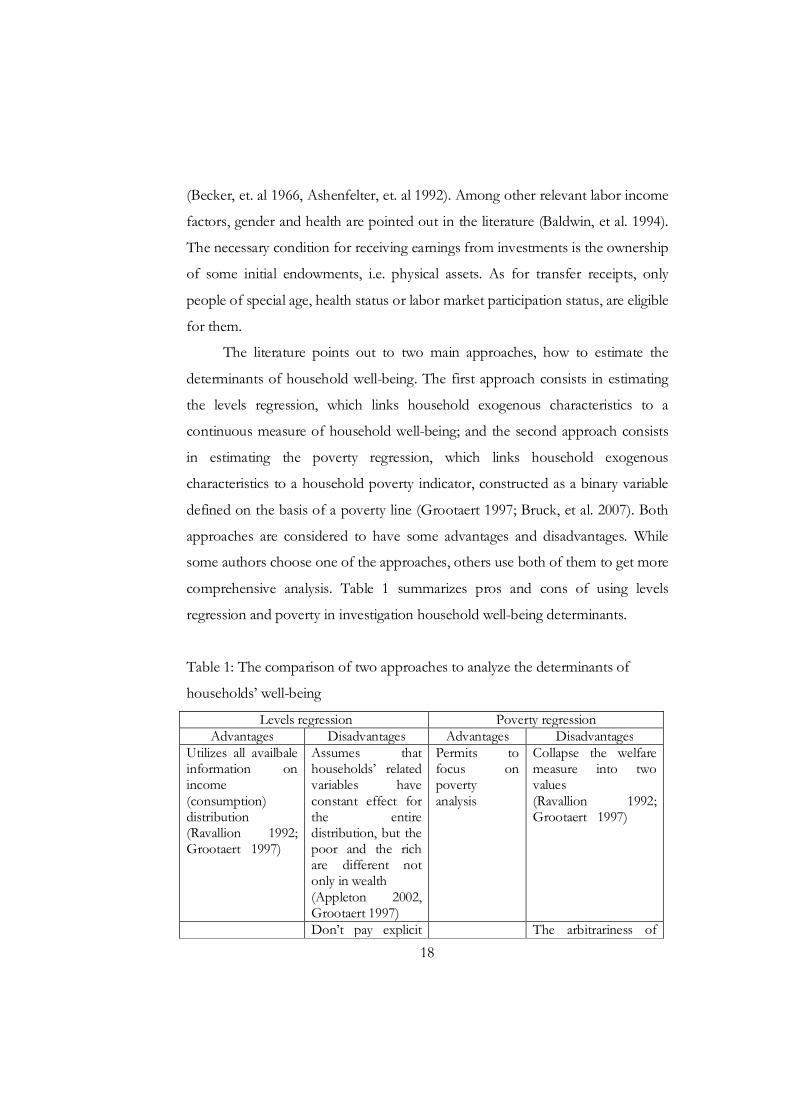
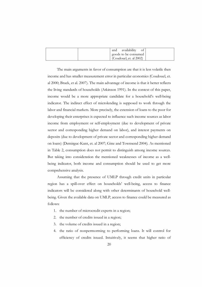
Table 1: The comparison of two approaches to analyze the determinants of

households’ well-being

Levels regression Poverty regression Advantages Disadvantages Advantages Disadvantages

Utilizes all availbale information on income (consumption) distribution (Ravallion 1992; Grootaert 1997)

Assumes that households’ related variables have constant effect for the entire distribution, but the poor and the rich are different not only in wealth (Appleton 2002, Grootaert 1997)

Permits to focus on poverty analysis

Collapse the welfare measure into two values (Ravallion 1992; Grootaert 1997)

Don’t pay explicit The arbitrariness of

19

attention to the poor and outliers (Baulch, et. al 2003)

the poverty line (Grootaert 1997; Coudouel, et. al 2002)

The choice of the dependent variables for both levels and poverty

regressions is not an easy one. There are numerous dimensions of well-being, i.e.

income, consumption, assets ownership, education and health (Coudouel, et. al

2002). The first two, income and consumption, are the most popular. Most

poverty researchers prefer consumption to income as a well-being indicator, or

they use them both and then compare the results. The comparison of two

household’s well-being indicators is presented in Table 2.

Table 2: The comparison of two main approaches to measure households’ well-

being

Income Consumption Advantages Disadvantages Advantages Disadvantages

Better proxy for living standards as it measures the opportunity for consumption opened to family (Atkinson 1991)

Measured over short periods, over/underestimates standards of living due to considerable variations in income over time (Bruck, et al. 2007)

Better indicator of general well-being as it is smoothed over time (Bruck, et al. 2007; Coudouel, et. al 2002)

Does not permit to distinguish among sources of income (Coudouel, et. al 2002)

Underestimates standards of living as people are less willing to reveal income than consumption (Datt, et al. 2000)

Has smaller measurement error for households living in poor agrarian economies or urban economies with large informal sector (Bruck, et al. 2007; Coudouel, et. al 2002)

Underestimates standards of living due to difficulties in quantifying earnings from self-employment (Datt, et al. 2000)

Reflects the access to

20

and availability of goods to be consumed (Coudouel, et. al 2002)

The main arguments in favor of consumption are that it is less volatile then

income and has smaller measurement error in particular economies (Coudouel, et.

al 2000; Bruck, et al. 2007). The main advantage of income is that it better reflects

the living standards of households (Atkinson 1991). In the context of this paper,

income would be a more appropriate candidate for a household’s well-being

indicator. The indirect effect of microlending is supposed to work through the

labor and financial markets. More precisely, the extension of loans to the poor for

developing their enterprises is expected to influence such income sources as labor

income from employment or self-employment (due to development of private

sector and corresponding higher demand on labor), and interest payments on

deposits (due to development of private sector and corresponding higher demand

on loans) (Demirguc-Kunt, et. al 2007; Gine and Townsend 2004). As mentioned

in Table 2, consumption does not permit to distinguish among income sources.

But taking into consideration the mentioned weaknesses of income as a well-

being indicator, both income and consumption should be used to get more

comprehensive analysis.

Assuming that the presence of UMLP through credit units in particular

region has a spill-over effect on households’ well-being, access to finance

indicators will be considered along with other determinants of household well-

being. Given the available data on UMLP, access to finance could be measured as

follows:

1. the number of microcredit experts in a region;

2. the number of credits issued in a region;

3. the volume of credits issued in a region;

4. the ratio of nonpermorming to performing loans. It will control for

efficiency of credits issued. Intuitively, it seems that higher ratio of

21

nonperforming to performing loans have no influence on average

household income (consumption), as nonperforming loans are

associated with unsuccessful projects, which have not contributed in

private sector development in a region and increase in demand for

labor.

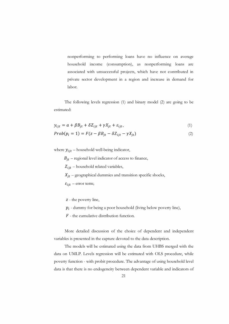
The following levels regression (1) and binary model (2) are going to be

estimated:

푦 = 푎 + 훽퐵 + 훿푍 + 훾푋 + 휀 , (1)

푃푟표푏(푝 = 1) = 퐹(푧 − 훽퐵 − 훿푍 − 훾푋 ) (2)

where 푦 – household well-being indicator,

퐵 – regional level indicator of access to finance,

푍 – household related variables,

푋 – geographical dummies and transition specific shocks,

휀 – error term;

푧 - the poverty line,

푝 - dummy for being a poor household (living below poverty line),

퐹 - the cumulative distribution function.

More detailed discussion of the choice of dependent and independent

variables is presented in the capture devoted to the data description.

The models will be estimated using the data from UHBS merged with the

data on UMLP. Levels regression will be estimated with OLS procedure, while

poverty function - with probit procedure. The advantage of using household level

data is that there is no endogeneity between dependent variable and indicators of

22

access to finance (banks penetration does not depend on wealth status of a

particular household but on average wealth status in a region). Nevertheless, there

is another potential problem for estimations. As explanatory variable data drawn

from a population with grouped structure (geographical location), the regression

errors could be correlated within groups (Moulton 1986, Moulton 1990). In this

case the assumption of independent errors is incorrect and the ordinary OLS

estimates will be biased. Thus, OLS standard errors will be adjusted for

intraregion correlation.

There is a rapidly expanding empirical quantile regression literature in

economics, which advocates using conditional quantile function to capture

different effect of explanatory variables across entire distribution (Koenker and

Hallock 2001). Thus, the analysis will be finished with estimation of a quantile

regresion to address the question whether improved access to finance has

different effect on households from different income groups.

23

C h a p t e r 4

DATA DESCRIPTION

The Ukrainian Microlending Program (UMLP)

UMLP is the only program in Ukraine that provides small loans for the

poor households to develop their enterprises. UMLP was established by the

European Bank for Reconstruction and Development and the German-Ukrainian

Fund in 1997. Raiffeisen Bank Aval (former Aval) was the first bank that joined

the program in Appril 1997. Initially, there were only four micro lending officers

that operated in Kyiv. Ggradually, other banks have joined the program: Privat

Bank (1997), Forum (2000), ProCredit Bank (former Microfinance Bank) (2001),

Nadra Bank (2002), CreditPrombank (2004). The youngest UMLP partner-banks

are Kredobank, Rodovid and Megabank (2007). Till recently, nine banks were

participating in the ULMP, providing microloans all over Ukraine. More detailed

history of this program is publicly available on its website

http://microcredit.com.ua.

The focus of this research is the indirect effect of microloans provision by

UMLP on households’ well-being in regions. To measure this effect, the access to

microloans in a region should be measured somehow. The dataset provided by

the UMLP includes monthly data on the number of experts operating in the

banks-participants, the number and volume of loans issued, and the number and

volume of overdue loans. This monthly data is specified for each region and

covers the period from the very beginning of the program (Appril, 1997) till

January, 2008. Using this dataset, three quantative and two qualitative indicators

are built in order to measure access to microloans in regions. They are as follows:

1. The number of UMLP experts operating through bank-participants of

the program. This indicator is built as a median of the number of

24

experts during the year in a region. This approach guarantees integers11

for persons (in contrast to mean values) and does not generate missing

values (in contrast to picking the number of experts in the beginnign

of the year).

2. The number of loans issued durgin a year. Calculated as the sum of

monthly loans issued in a region.

3. The volume of loans issued during a year. Calculated the same way as

the previous indicator, with only difference that it is in hryvnias.

4. The ratios of nonperforming loans to performing loans. Two

qualitative ratios could be built, using the data separatley on the

number of loans and on the volume of loans. These ratios will control

for the quality of loans issued. It is assumed that if loan is

nonperforming, the poor client have not managed to develop his

bussines yet, and thus the loan made to him have not created positive

spill-over effect on household’s well-being in this region. The number

and volumes of performing and nonperforming loans are provided

cummulatively per each month. Nonperforming loans are overdue

loans for 15, 30, 60 and more days. To calculate qualitative ratios for

each year, first, the ratios are calculated for each month. Then, the

median value of monthly ratios are chosen as the ratio for the current

year.

If the UMLP is not presented in the region, each of this indicators is taken

as zero. All the indicators are annual, for the period 1997-2007, and specified for

each region.

To see, how UMLP have been expending in Ukraine, each indicator was

calculated for the whole country by taking the median value of regional indicator

for each year. The dynamic of access to finance indicators are presented on 11 However, in data from UMLP the monthly number of experts sometimes have decimal point equal to 5,

which could mean that the an expert was hired (fired) during the month.

25

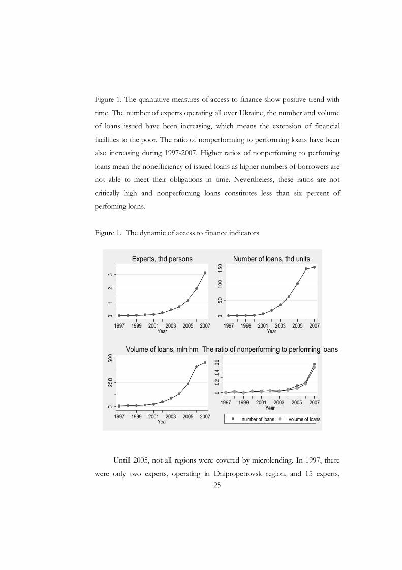
Figure 1. The quantative measures of access to finance show positive trend with

time. The number of experts operating all over Ukraine, the number and volume

of loans issued have been increasing, which means the extension of financial

facilities to the poor. The ratio of nonperforming to performing loans have been

also increasing during 1997-2007. Higher ratios of nonperfoming to perfoming

loans mean the nonefficiency of issued loans as higher numbers of borrowers are

not able to meet their obligations in time. Nevertheless, these ratios are not

critically high and nonperfoming loans constitutes less than six percent of

perfoming loans.

Figure 1. The dynamic of access to finance indicators

Untill 2005, not all regions were covered by microlending. In 1997, there

were only two experts, operating in Dnipropetrovsk region, and 15 experts,

01

23

1997 1999 2001 2003 2005 2007Year

Experts, thd persons

050

100

150

1997 1999 2001 2003 2005 2007Year

Number of loans, thd units

025

050

0

1997 1999 2001 2003 2005 2007Year

Volume of loans, mln hrn

0.0

2.0

4.0

6

1997 1999 2001 2003 2005 2007Year

number of loans volume of loans

The ratio of nonperforming to performing loans

26

operating in Kyiv region. In 1998, microlending covered two additional regions –

Lvivskyi and Zaporizhskyi. The last regions, which were covered only in 2005,

were Chernihivskyi region and Kirovohradskyi region. The detailed statistics on

experts penetration over regions in 1997-2007 is presented in the Appendix,

Table 8. There are a lot of experts in Dnipropetrovkyi, Donetskyi, Kyivskyi,

Lvivskyi and Crimea regions. These regions are known as highly populated and

much economically active.

If regions are aggregated in four geographical groups, i.e. north, south, west

and east regions, it appears that in 2007 UMLP experts have penetrated regions

propotionally to population. According to the diagram on Figure 2, in 2007

34.17% of experts were operating in east regions, 27.9% - in west regions,

22.48% - in north regions and 15.46% - in south regions. Correspondingly,

34.85% of Ukrainian population lives in the east, 26.83% – in the west, 23.11% -

in the north and only 15.21% - in the south. Thus, by 2007 miclolending has been

presented uniformly over Ukraine.

The Table 10 in the Appendix presents the summary statistics on

indicators of access to microloans in regions for the period 1997-2007. Those

regions, where the program were not presented at some points of time, are not

taken into account for calculation of these statistics. After merging this dataset

with the micro level data on households, indicators on access to microloans in a

region not covered by the UMLP in that time are set to zero.

The Ukrainian household budgeting survey (UHBS)

UHBS was introduced by the Cabinet of Ministers of Ukraine in 1998

(Enactment №1725 from 1998, November 2). The aim of this survey is to create data

base for detailed analysis of living standards of Ukrainian population and poverty

evaluation. UHBS provides with detailed information on socioeconomic characteristics

of households from a representative sample, i.e. households’ income and expenditures,

labor market participation, education, health status, assets and others. The survey is

27

conducted each quarter12, starting from 1999, and in line with world standards and

modern scientific researh. However, methodology of building a sample was approved

only in 2005, by Decree №223 of State Statistics Committee of Ukraine. According

to this Decree, the sample is

built in two stages. On the first stage, administrative-territorial units are chosen

and not changed during 5 years. On the second stage, addresses of households

are chosen. This sample dimention is changed each year.

Figure 2. The penetration of the UMLP by regions in 2007

Using the available sample of households, the sets of dependent and

explanatory variables are built. The former set includes income, consumption and

two corresponding poverty lines.

12 However, the data available for the analysis is an annual one and for the period starting from the year 2000

to the year 2007

15.46%

22.48%

27.9%

34.17%

soth northwest east

Penetraion of experts by regions, 2007

15.21%

23.11%

26.83%

34.85%

Source: State Statistics Committe of Ukraine

Penetraion of population by regions, 2007

28

In empirical poverty literature income is considered in a family context

under the assumption that all income is pooled and shared by all members

(Finnie, et. al 2003). The UHBS provides with data on both monetary and inkind

income received during a year by all household members. Among income

generating sources are after-tax wages, income from individual labor activities and

from sale of home produced goods, dividends, interest payments, property rents,

pensions, scholarships, unemployment payments and other social allowances,

subsidies and facilities, help and gifts, alimony and different arrears payments

(arrears of wages, pensions, scholarships and allowances). Household income also

includes the value of home produced and consumed food.

After summation of all these income sources, in order to make households’

well-being and poverty indicators comparable, firstly, the value of income is

deflated by the household size. The calculation of per capita income or

consumption is based on the assumption of economies of scale in family

consumption (Finnie, et. al 2003; Grootaert 1997; Kislitsyna 2003; Datt, et. al

1999). As large households can benefit from sharing commodities and utilities,

and from purchasing goods in bulk, household’s members are usually assigned

different weights (Coudouel, et. al 2002). The set of these weights is referred to as

the equivalence scale and there is no single agreed-on one (OECD Social Policy

Division n.d.). For example, Kislitsyna (2003) uses the equivalence scale of the

Organization of Economic Cooperation and Development (OECD), according

to which the household head has weight equal to 1, each other adult – 0.7, and

each child – 0.5. The household head is a family member who brings in the

highest share of total household income13, while children are the offspring of the

head (and/or spouse) irrespective of age (de Vos and Zaidi 1997). Finnie, et. al

(2003) refer to an increasingly common adjustment rule of square root.

13 In case of equal income but different sex, the household head is a male, in case

of equal income and the same sex, the household head is the older one (Kislitsyna 2003)

29

According to the square root rule, the household’s total income is divided by the

square root of household size, thus implying that the needs of a household of

four member is only twice as large as the needs of a household of one member.

Datt, et al. (2000) assumes no economies of household size and weights each

household member as 1.

For this research, individual income and consumption are calculated with

the equivalence scale, which reflects the economy of scales in consumption for

Ukrainian households and in accordance with the Methodology of integrated

evaluation of poverty in Ukraine (approved by Enactement

№171/238/100/149/2нд from 2002, April 5). This Methodology gives a

household head the weight equal to 1, but each other member – 0.7. The exact

formula to adjust household’s income and consumption for household size is

as follows:

푦 =. ( )

(3)

where 푦 – income or consumption per capita;

푌 – household income or consumption;

푁– household size.

Secondly, income should be adjusted for differences in prices across

regions and at different points in time (Coudouel, et. al 2002). Unfortunetely,

there is no data on regional price levels for Ukraine. For this reason, this research

relies only on national consumer price index (CPI), which could suffer from

regional biases (Bruck, et al. 2007). As income is an annual measures, it is deflated

by annual CPI to the year 2000.

Consumption measure reflects the value of all items, which were consumed

or spent money on during a year. These items involves food, drinks, clothes and

footwear, furniture, different services including utilities, education, recreation and

entertainment, renovation, help, alimony and others. The value of items,

30

produced at home or received free, and then consumed is also included in

expenditures. Input and investment expenditures are excluded from

consumption. Including such spending in the consumption leads to

overestimation of the actual welfare levels achieved by households (Coudouel, et.

al 2002). The total value of consumption is deflated by household size and CPI

index the same way as income.

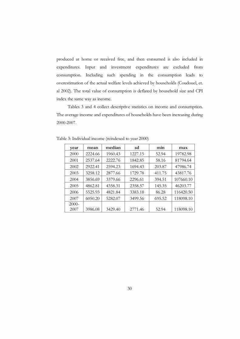
Tables 3 and 4 collect descriptive statistics on income and consumption.

The average income and expenditures of households have been increasing during

2000-2007.

Table 3: Individual income (reindexed to year 2000)

year mean median sd min max 2000 2224.66 1960.43 1227.15 52.94 19782.98 2001 2537.64 2222.76 1842.85 58.16 81794.64 2002 2922.41 2594.23 1694.43 203.87 47986.74 2003 3258.12 2877.66 1729.78 411.75 43817.76 2004 3856.69 3379.66 2296.61 394.51 107660.10 2005 4862.81 4358.31 2358.57 145.35 46203.77 2006 5525.93 4821.84 3383.18 86.28 116420.50 2007 6050.20 5282.07 3499.56 695.52 118098.10 2000-2007 3986.08 3429.40 2771.46 52.94 118098.10

31

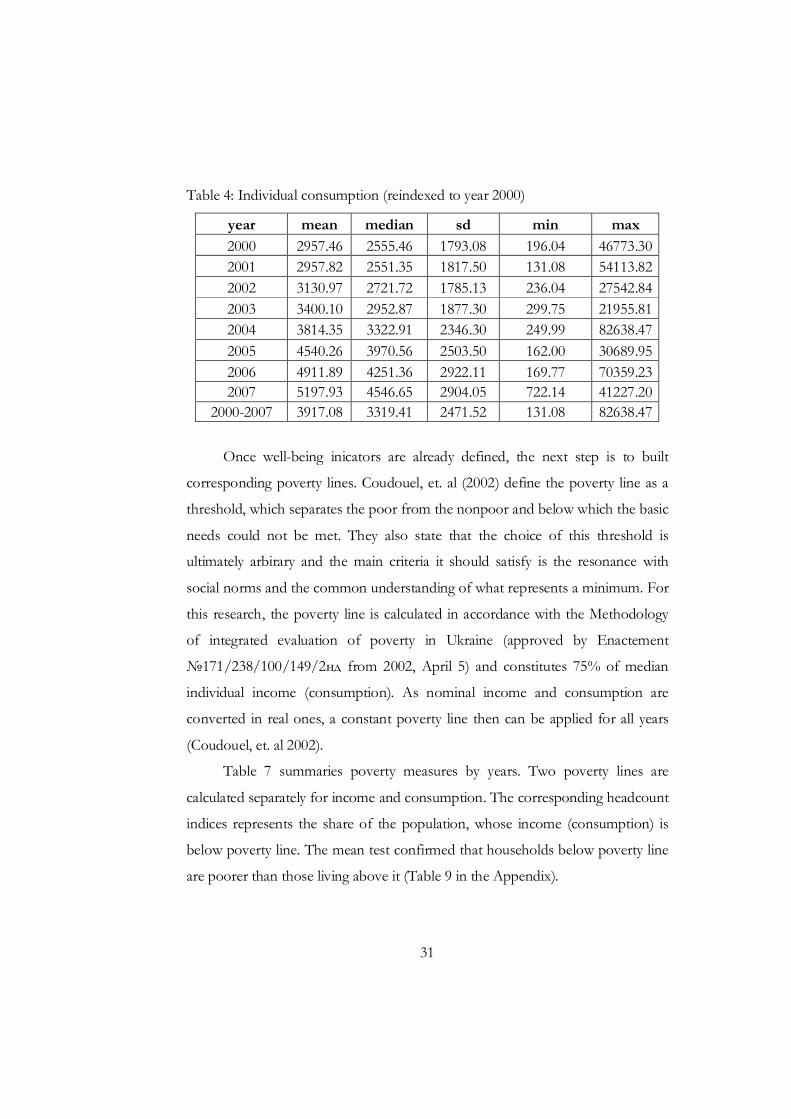
Table 4: Individual consumption (reindexed to year 2000)

year mean median sd min max 2000 2957.46 2555.46 1793.08 196.04 46773.30 2001 2957.82 2551.35 1817.50 131.08 54113.82 2002 3130.97 2721.72 1785.13 236.04 27542.84 2003 3400.10 2952.87 1877.30 299.75 21955.81 2004 3814.35 3322.91 2346.30 249.99 82638.47 2005 4540.26 3970.56 2503.50 162.00 30689.95 2006 4911.89 4251.36 2922.11 169.77 70359.23 2007 5197.93 4546.65 2904.05 722.14 41227.20

2000-2007 3917.08 3319.41 2471.52 131.08 82638.47

Once well-being inicators are already defined, the next step is to built

corresponding poverty lines. Coudouel, et. al (2002) define the poverty line as a

threshold, which separates the poor from the nonpoor and below which the basic

needs could not be met. They also state that the choice of this threshold is

ultimately arbirary and the main criteria it should satisfy is the resonance with

social norms and the common understanding of what represents a minimum. For

this research, the poverty line is calculated in accordance with the Methodology

of integrated evaluation of poverty in Ukraine (approved by Enactement

№171/238/100/149/2нд from 2002, April 5) and constitutes 75% of median

individual income (consumption). As nominal income and consumption are

converted in real ones, a constant poverty line then can be applied for all years

(Coudouel, et. al 2002).

Table 7 summaries poverty measures by years. Two poverty lines are

calculated separately for income and consumption. The corresponding headcount

indices represents the share of the population, whose income (consumption) is

below poverty line. The mean test confirmed that households below poverty line

are poorer than those living above it (Table 9 in the Appendix).

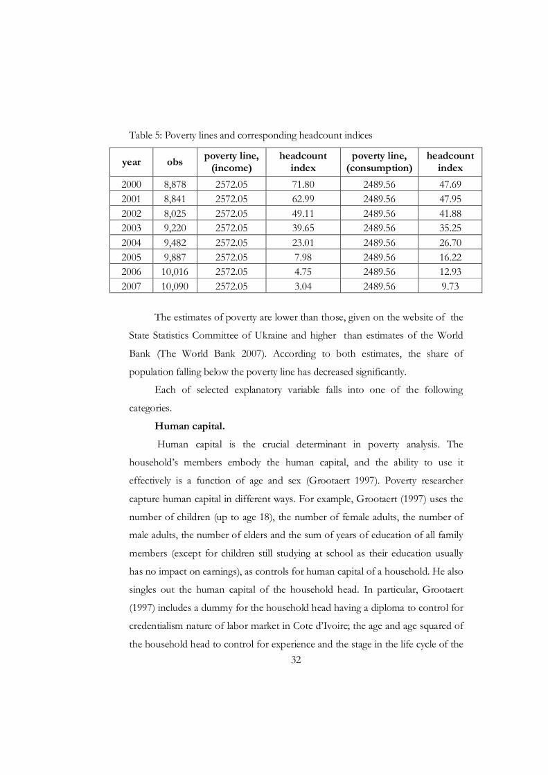
32

Table 5: Poverty lines and corresponding headcount indices

year obs poverty line, (income)

headcount index

poverty line, (consumption)

headcount index

2000 8,878 2572.05 71.80 2489.56 47.69 2001 8,841 2572.05 62.99 2489.56 47.95 2002 8,025 2572.05 49.11 2489.56 41.88 2003 9,220 2572.05 39.65 2489.56 35.25 2004 9,482 2572.05 23.01 2489.56 26.70 2005 9,887 2572.05 7.98 2489.56 16.22 2006 10,016 2572.05 4.75 2489.56 12.93 2007 10,090 2572.05 3.04 2489.56 9.73

The estimates of poverty are lower than those, given on the website of the

State Statistics Committee of Ukraine and higher than estimates of the World

Bank (The World Bank 2007). According to both estimates, the share of

population falling below the poverty line has decreased significantly.

Each of selected explanatory variable falls into one of the following

categories.

Human capital.

Human capital is the crucial determinant in poverty analysis. The

household’s members embody the human capital, and the ability to use it

effectively is a function of age and sex (Grootaert 1997). Poverty researcher

capture human capital in different ways. For example, Grootaert (1997) uses the

number of children (up to age 18), the number of female adults, the number of

male adults, the number of elders and the sum of years of education of all family

members (except for children still studying at school as their education usually

has no impact on earnings), as controls for human capital of a household. He also

singles out the human capital of the household head. In particular, Grootaert

(1997) includes a dummy for the household head having a diploma to control for

credentialism nature of labor market in Cote d’Ivoire; the age and age squared of

the household head to control for experience and the stage in the life cycle of the

33

household. Bokosi (2007) represents household composition with the total

number of household members as well as the number of family member below

10 years old and above 60 years old. As for education level, Bokosi (2007)

controls only for education of the household head, including dummy variables

for attending primary school, secondary school or no formal education at all into

regression. Similar to Grootaert (1997), Bokosi (2007) includes the age and age

squared of the household head among other human capital controls. The

distinctive features of Datt, et al. (2000) approach to capture human capital are as

follows: he takes household size squired (in order to allow for nonliniarity in the

household size living-standards relationships), distinguishes four main age

categories (under 10, 10-17, 18-59 and 60) and splits the number of productive

age adults in the 18-59 age-group by gender. For education, Datt, et. al (2000)

includes the maximum level of education attained by one of family members as

well as the number of literate family members, the number of family members

with primary or higher level of education. Lastly, in contrast to Grootaert (1997)

and Bokosi (2000), Datt, et. al (2000) does not control for the household’s stage

in the life cycle. All three researchers Grootaert (1997), Bokosi (2000) and Datt,

et. al (2000) put a dummy for the gender of the household head to control for

market discrimination and segmentation.

To analyse poverty determinants in Ukraine, Bruck, et al. (2007) propose to

capture human capital with household size (in log), average years of schooling

and the share of family members in one of the age groups (0-14, 15-25, 41-

pension age, after pension age). Such age composition is argued to affect the

distribution of different income sources in Ukraine.

For this research, the household size, average years of schooling, the

number of children and the number of elders are used to control for human

capital. Children are family members younger than 14 years old. This age range is

chosen, as children of this age could prevent matured family members from labor

market participation activities and require more time to take care of. Elders are

34

women after 55 and men after 60 years old. Most family members that belong to

this age category are retired and receive pension benefits. UHBS does not provide

data to distinguish students (aged 15-25), people in the beginning of their career,

from adults with great work experience (41-pension age). Instead of these two

age groups, the number of employed family members will be included in the

regression. The use of the number of members in the age group instead of their

share is motivated by convenience of interpretation and more frequent use by

other poverty researchers (Grootaert (1997), Bokosi (2007), Datt, et al. (2000)).

Average years of education control for education level of family member in

working age (starting from 16 according to the Ukrainian law). UHBS provides

with categorical information on education of family members, distinguishing

eight categories as follows:

1. Nonliterate family member,

2. Family member without primary school education,

3. Family member with primary school education,

4. Family member with secondary school education,

5. Family member with high school education,

6. Family member with unfinished degree,

7. Family member with one-two years degree,

8. Family member with four year degree and higher.

These categories are presented in ascending order as a proxy for years of

schooling. Average years of schooling for a household is received by the

summation of total years of schooling of household members in the working

age, divided by their number.

Physical capital.

Physical capital is another important determinant of household’s well-

being, as it determines the household’s possibility to generate income through

own activity or smooth consumption, and links the household with the labor

market (Grootaert 1997,). Datt, et. al (2000) captures physical capital with the

35

total area of landholding and a dummy for the possession of a particular type of

livestock no less than the 75th percentile among households who own at least one

of that type of livestock. Similarly, Bokosi (2007) includes the natural log of per

capita livestock owned and per capita acreage cultivated into regression. In

contrast to Datt, et. al (2000) and Bokosi (2007), Grootaert (1997) controls for

variety of assets owened by a household. They are the amount of farmland, the

value of farm equipment, the value of non-farm stocks and equipment, durable

goods and ownership of home the household live in.

Bruck, et. al (2007) use two dummies for possession of land and car in

previous period as proxies for cummulative wealth status of a household or

ability to generate inome through home-production activity. UHBS does not

specify data on households assets in periods prior to study. The alternative way to

set the link between productive assets and poverty is to include the share of

income sources (Grootaert (1997)). Thus, the ownership of productive assets is

captured with the share of agricultural income (including plant cultivation, poultry

faming, livestock farming and bee-farming).

Geographical dummies.

Locale of a household is an agreed-on determinant of a household well-

being. In Ukraine, they are proxy for industry structure (Bruck, et. al 2007). Both

the settlement type (village, town, city) and macro-regions (north, east, south,

west and capital Kiev) are controlled with correspondent dummies.

Transition specific shocks.

Bruck, et. al (2007) point out to the transition specific shocks as

determinants of poverty in Ukraine. Thus, two dummies for the transition

specific shocks are also included into regression. The first one is the inkind

payment (equal to one if one of the family members has received inkind wage)

and the second one is the unemployment (equal to one if one of the family

members has had a status of being unemployed).

36

In the long run such variables as household size or physical assets are

endogeneus to household wealth, while in one-year analysis they could be treated

as given (Grootaert 1997). Given the cross-section nature of the data provided by

the UHBS, the mentioned variabls are considered as exogenous for the further

analysis.

Descriptive statistics for all variables is presented in Tables 11-12 in the

Appendix. Income and consumption are loglinearised. Table 12 presents the

descriptive statistics on the indicators of access to microloans in a region, after

they were merged with the data file on households. All nominal variables are

expressed in 2000 hryvnias using the national CPI index, provided by the State

Statistics Committee of Ukraine. Intuition behind estimating the effect of lagged

indicators is as follows. After loans are approved and made to a household, it

takes time to establish and develop a business, hire additional worker and so on.

Thus, the spill-over effect should be estimated not earlier than a next year.

37

C h a p t e r 5

MULTIVARIATE REGRESSIONS RESULTS

OLS regressions

Tables 13-15 in the Appendix show regression results for determinants of

household well-being in 2000-2007, measured by income and consumption. For

estimation and interpretation convenience the number of experts is express in

tens of persons, the number of loans issued – in thousands of units and the

volume of loans issued – in million of hryvnias. The relevant goodness-of-fit

statistics shows the good fit for all model specifications.

Table 6 summarizes the estimated coefficients of variables that are in the

focus of this research, i.e. regional indicators of access to microloans. The

choice of household well-being indicator (income or consumption) has an

effect on estimates and the conclusions that one can draw regarding the impact

of improved access to finance on household well-being in Ukraine. According

to the results, the coefficients on quantitative indicators are positive and

significant for regressions with income as a dependent variable, in particular:

1. An increase in issued loans in a region by one thousand is associated with

an increase in an average income by 0.5% next year, 0.6% two years after,

and 0.9% three years after.

2. An increase in the volume of loans issued in a region by one million

hryvnias is associated with an increase in an average income by 0.1% next

year, 0.2% two years after, and 0.3% three years after.

3. An increase in the number of experts operating in a region is associated

with an increase in an average income by 0.4% next year, 0.5% two years

after, and 1.00% three years after.

38

All coefficients on quantitative indicators of access to microloans are

positive, but insignificant for regressions with consumption as a dependent

variable.

The coefficients on the ratio of nonperforming to performing loans is

also positive, but mostly insignificant for different regression specifications.

These ratios should have been measured more properly if there were better

information about credit portfolios.

Coefficients on other variables are mostly as expected. There is a strong

effect of household composition on its well-being level. Number of children

exhibit negative and significant effect on individual income, while insignificant

effect on individual consumption. Having a family member in the pension age

significantly increase individual income and consumption, which is attributed to

the pesion increase in Ukraine (Bruck, et al. 2007). Households with employed

family members also enjoyes higher income and consumption. There is a strong

gender effect, i.e. female-only households suffer from lower income and

consumption. Higher level of education benefits household in terms of both

income and consumption: an additional average year of schooling is associated

with 7% gain in average income and 8.6% gain in average consumption per

person. Bruck, et al. (2007) points out to increasing returns to human capital in

Ukraine.

Ownership of productive assets proxied by the share of farm income has

a positive and significant impact on income and consumption, showing the

importance of subsistence agriculture as a source of income for households in

Ukraine.

There is also an effect of geographical location on household well-being.

Houeholds residing in towns and villages are worse off than households living

in cities, however, the effect of villages is insignificant for income. Households

residing in any marco-region has a significant disadvange in terms of income

and consumption in comparison to households residing in the capital of Kiev.

39

There is a negative effect of transition shocks on households well-being,

i.e. households that are exposed to unemployment or inkind payment shocks

have lower income and consumption.

Dummies for years are positive and strongly significant.

Thus, according to the results from level functions estimation, there is an

indirect effect from improved access to finance on households income. The

robustness of results could be checked with probit regressions. The quantile

regression will be valuable to address the question whether improved access to

finance has different effects on households from different income groups.

Probit regressions

Tables 16-18 in the Appendix present the regression results for

determinants of household probability to fall into poverty.

Table 7 summarizes marginal effects of access to finance indicators

received from estimation of poverty functions. They are in line with results

from welfare functions estimation.

1. An increase in issued loans in a region by one thousand is associated

with a decrease in probability to be poor by 0.005 next year, 0.006 two

years after, and 0.009 three years after.

2. An increase in volume of loans issued in a region by one million

hryvnias is associated with a decrease in probability to be poor by

0.002 next year, 0.002 two years after, and 0.004 three years after.

3. An increase in the number of experts operating in a region is

associated with a decrease in probability to be poor by 0.004 next year,

0.007 two years after, and 0.013 three years after.

Again, the ratios of nonperforming loans to performing loans are

insignificant for most specifications.

40

Marginal effects of other poverty determinants are consonant with

estimations of levels function.

Human capital is an important determinant of household probability to fall

into poverty. In particular, household size, number of children and being only a

female household increase the probability to be poor, while number of employed

family members, number of elders and additional year in average years of

schooling decrease the probability to be poor. Having a productive assets

decrease the probability of household to fall into poverty. Transition specific

shocks, inkind payments and unemployment, have a significant positive effect on

household probability to be poor. Residing in village or town has a positive

significant effect on the probability to be poor in consumption, but insignificant

effect on the probability to be poor in income. Residing in regions different from

the capital of Kiev significantly increase the probability to be poor. According to

estimated effects of year dummies, each year the probability to be poor decrease.

Quantile regression

Table 19 in the Appendix shows the quantile regression of income on the

set of explanatory variables for the 10th, 25th, 50th, 75th, and 90th percentiles. The

access to finance indicators are the number of loans and the ratio of performing

to nonperforming loans with, taken with three lags.

One of the remarkable results concerns the quantitative indicator of

access to finance. The effect of it is higher at higher percentiles. The qualitative

indicator is positive and significant, and has highest effect on the households

with the median level income and below it.

Interesting results are on the effects of household human capital

indicators. For the less well-off households the household size has smaller

negative effect on income. Having more children has no effect for rich

households (0.9 percentile). Having more employed family members and elders

41

has higher positive effect on income of poorer households. Average years of

schooling and ownership of productive assets have higher effect on richer

households. Female-only households are worse-off and this gender factor has

higher effect at higher quantiles of income distribution. As for transition

specific shocks, the results are similar to those reported above, but it should be

mentioned that the poor are more sensitive to them. In terms of geographical

location, similar patterns are observed as before, with the only difference that

location has higher effect on less poor households. Residing in a village has no

effect on the households with income from the lower quantiles. Time positively

effects household income from entire distribution, but has higher effect on

poorer households.

42

Table 6: Estimated effect of microlending with levels regressions

Number of loans Volume of loans Number of experts Lags Ln of

income Ln of

consumption Ln of

income Ln of

consumption Ln of

income Ln of

consumption Lag 1 0.005***

(3.76) 0.003 (0.91)

0.001*** (3.98)

0.001 (1.05)

0.004*** (3.68)

0.002 (0.81)

Lag 2 0.006*** (3.05)

0.003 (0.6)

0.002*** (3.26)

0.001 (0.79)

0.005*** (3.36)

0.002 (0.6)

Lag 3 0.009*** (3.44)

0.005 (0.91)

0.003*** (4.67)

0.002 (1.26)

0.010*** (3.98)

0.006 (1.15)

Number of nonperforming loans to performing

Volume of nonperforming loans to performing

Number of nonperforming loans to performing

Lag 1 1.384** (2.57)

1.713 (1.42)

0.864 (1.20)

0.534 (0.52)

1.483*** (2.78)

1.797 (1.53)

Lag 2 1.863*** (5.20)

1.896** (2.52)

1.159 (1.16)

0.882 (0.82)

1.795*** (5.57)

1.919** (2.55)

Lag 3 1.071 (1.61)

0.713 (1.03)

-0.482 (0.75)

-0.466 (0.64)

0.826 (1.46)

0.550 (0.83)

43

Table 7: Estimated effect of microlending with poverty functions

Number of loans Volume of loans Number of experts Lags Poverty line

based on income

Poverty line based on

consumption

Poverty line based on income

Poverty line based on

consumption

Poverty line based on income

Poverty line based on

consumption Lag 1 -0.005***

(2.58) -0.003 (0.93)

-0.002*** (2.95)

-0.001 (1.03)

-0.004** (2.29)

-0.002 (0.61)

Lag 2 -0.006** (2.08)

-0.003 (0.68)

-0.002*** (2.72)

-0.001 (0.87)

-0.007*** (2.74)

-0.002 (0.43)

Lag 3 -0.009** (2.38)

-0.004 (0.75)

-0.004*** (3.78)

-0.002 (1.30)

-0.013*** (3.71)

-0.005 (1.01)

Number of nonperforming loans to performing

Volume of nonperforming loans to performing

Number of nonperforming loans to performing

Lag 1 -1.894*** (3.95)

-1.720 (1.61)

-0.737 (0.76)

-0.476 (0.50)

-1.919*** (4.08)

-1.869* (1.83)

Lag 2 -1.933*** (4.21)

-1.518** (2.53)

-0.971 (1.16)

-0.379 (0.38)

-1.766*** (4.51)

-1.593*** (2.63)

Lag 3 -0.566 (1.01)

-0.634 (1.00)

0.706 (1.53)

0.541 (0.80)

-0.220 (0.50)

-0.495 (0.81)

44

C h a p t e r 6

CONCLUSIONS

The impact of better financial inclusion of population on poverty

outcomes is subject to a lot of research. Some authors report the success of

microfinance in poverty reduction, while others still remain skeptic.

Using micro level data on households and regional access to finance

indicators, built with the data provided by the UMLP, the spill-over effect of

microlending expansion in Ukraine was analyzed. Evidence was presented that

there is an indirect effect of microlending on households’ income in Ukraine.

However, there is no observable effect on households’ consumption. The spill-

over effect is higher on the second and third years after loans were issued. It is

explained by UMLP contribution into private sector development and

corresponding increase in households’ labor income.

According to estimation results, the size of the effect is not very high.

The microlending expansion Ukraine explains no more than 1% increase in

average annual income per capita, which could be explained with the middle run

of microlending expansion.

The analysis with a quantile regression showed that the indirect effect of

microlending is positive for households at the entire distribution, but the effect

is higher at the top of it.

The assessment of the effect of improved access to finance on households’

well-being in a transition country, the use of UMLP data to measure access to

finance and the concentration on the indirect effect of microfinance makes this

research different.

45

Appendix

Table 8: The median number of UMLP experts by regions, 1997-2007

Regions 1997 1998 1999 2000 2001 2002 2003 2004 2005 2006 2007 Cherkasy - - - - - - 3 5.5 16.5 43 79 Chernihiv - - - - - - - - 7 17.5 47.5 Chernivtsi - - - - 1 7 16.5 25 49.5 70 104 Crimea - - - 4 5 8 13 20 44 116.5 162.5 Dnipropetrovsk 2 4 7.5 12 14.5 33 57.5 87.5 143 228 330.5 Donetsk - - 2 3 5 30.5 63.5 90 126 194 260.5 Ivano-Frankivsk - - - - - 1 5 6.5 6.5 34.5 97.5 Kharkiv - - 3 3 4.5 21.5 31 37.5 49 72 137.5 Kherson - - - - 1 8.5 19 27 60.5 87 89.5 Khmelnytskyi - - - 1.5 4 8.5 19 26.5 42.5 84.5 106.5 Kirovohrad - - - - - - - - 4.5 9 46 Kyiv 15 19.5 17 13 30 38 64 91 128.5 184 248 Luhansk - - - - 3 3.5 10.5 16 28.5 66.5 117 Lutsk - - - 3 2 4 7 14 23 61 115 Lviv - 4 10 9 13 19.5 33 49.5 74 130 195.5 Mykolaiv - - 2 2.5 5 9 18.5 35 56 77.5 109 Odessa - - - - - 10 23 30 54 91 119 Poltava - - - - - 2 4.5 7.5 28 65 104.5 Rivne - - - 1 3 5 10.5 20.5 28 38.5 88 Sumy - - - - - 1 4 5 9 14 77 Ternopil - - - - - - 7 13.5 22.5 38.5 94.5 Vinnytsia - - - - - - 7 15 22.5 39.5 97.5 Zakarpattya - - - - - 4 3 6.5 15.5 42.5 65.5 Zaporizhya - 2 6 8.5 9 14 23 29 62 100 138.5 Zhytomyr - - - - - - - 5 18.5 39.5 75.5

46

Table 9: T-test on the equality of income (consumption) means between poor and nonpoor households

Income Consumption

The nonpoor The poor The nonpoor The poor

2000 3689.13*** (1341.38)

1644.95*** (503.17)

4024.27*** (1891.85)

1790.44*** (442.25)

2001 3870.08*** (2473.4)

1756.65*** (483.94)

4063.98*** (1880.14)

1765.29*** (464.44)

2002 3913.53*** (1837.86)

1898.86*** (450.08)

4096.46*** (1843.5)

1820.91*** (443.14)

2003 4152.75*** (1889.87)

1997.10*** (400.77)

4304.44*** (1958.84)

1871.04*** (416.2)

2004 4479.01*** (2472.01)

2072.68*** (405.34)

4614.66*** (2427.69)

1923.34*** (416.27)

2005 5251.43*** (2501.58)

2064.85*** (397.82)

5163.55*** (2560.65)

1945.18*** (401.61)

2006 5801.29*** (3443.59)

2090.40*** (403.88)

5448.14*** (3015.91)

1990.19*** (385.56)

2007 6348.71*** (3687.45)

2093.71*** (376.09)

5633.73*** (2922.15)

2003.50*** (369.58)

2000-2007 5015.33*** (2934.07)

1831.90*** (486.98)

4797.78*** (2526.43)

1846.25*** (438.79)

47

Table 10: Descriptive statistics of regional access to finance indicators, 1997-2007

Variables Number of observations Mean Std. Dev. Min Max

Number of loans issued, thd. units 177 2.97 3.54 0.0010 17.07

Volume of loans issued, mln. hrns, reindexed to year 2000

177 13.93 16.85 0.01 91.82

Number of experts, tens of persons 177 4.38 5.49 0.10 33.05

Number of nonperfoming to perfoming loans

177 0.02 0.02 0 0.12

Volume of nonpermoning loans to perfoming loans

177 0.01 0.02 0 0.21

48

Table 11: Descriptive statistics of the data from UHBS, 2000-2007

Variables Obs Mean Std. Dev. Min Max Ln of income 74439 8.12 0.57 3.97 11.68 Ln of consumtpion 74439 8.12 0.55 4.88 11.32 Poverty line based on income 74439 0.31 0.46 0 1 Poverty line based on consumption 74439 0.29 0.45 0 1 Househod size, number of people 74439 2.49 1.32 1 14 Number of employed family members 74439 1.02 0.94 0 3

Number of children (0-14 years old) 74439 0.12 0.38 0 5 Number of elders (women older 55, men older 60) 74439 0.70 0.76 0 4

Average years of schooling 74439 5.07 1.40 1 8 Female-only household 74439 0.29 0.45 0 1 Share of farm income (a proxy for productive assets) 74439 0.16 0.23 0 25.49

Unemployment 74439 0.19 0.39 0 1 Inkind 74439 0.06 0.24 0 1 Village 74439 0.36 0.48 0 1 Town 74439 0.29 0.45 0 1 City 74439 0.35 0.48 0 1 Capital 74439 0.04 0.19 0 1 North 74439 0.24 0.43 0 1 West 74439 0.24 0.43 0 1 South 74439 0.15 0.36 0 1 East 74439 0.33 0.47 0 1 25 regions, Kiev and Sevastopol 74439 12.91 7.48 1 27 Year 74439 2003.64 2.30 2000 2007

49

Table 12: Descriptive statistics of regional access to finance indicators merged with data from UHBS, 2000-2007

Variable Obs Mean Std. Dev. Min Max Year 74439 2003.64 2.30 2000 2007 Regions 74439 12.21 6.93 1 25 Number of experts, lag1 74439 31.35 45.20 0 228 Number of experts, lag2 74439 18.92 29.44 0 143 Number of experts, lag3 74439 11.57 19.71 0 91 Number of loans, lag1 74439 2.57 3.74 0 17.07 Number of loans, lag2 74439 1.59 2.69 0 13.13 Number of loans, lag3 74439 0.91 1.78 0 9.55 Volume of loans, lag1 74439 11.33 16.43 0 80.99 Volume of loas, lag2 74439 6.84 10.76 0 49.27 Volume of loans, lag3 74439 4.19 7.35 0 36.84 Number of nonperforming loans to performing, lag1 74439 0.01 0.01 0 0.05 Number of nonperforming loans to performing, lag2 74439 0.01 0.01 0 0.04 Number of nonperforming loans to performing, lag2 74439 0.00 0.01 0 0.04 Volume of nonperforming loans to performing, lag1 74439 0.01 0.01 0 0.07 Volume of nonperforming loans to performing, lag1 74439 0.00 0.01 0 0.04 Volume of nonperforming loans to performing, lag1 74439 0.00 0.01 0 0.04

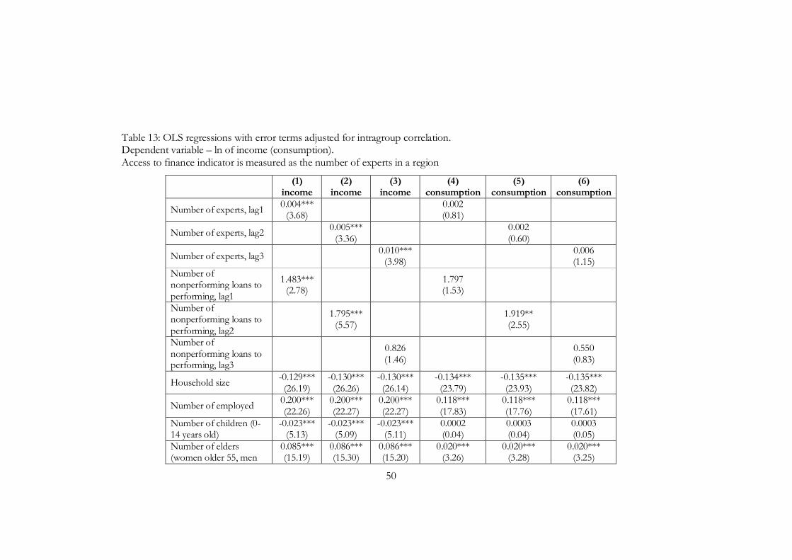
50

Table 13: OLS regressions with error terms adjusted for intragroup correlation. Dependent variable – ln of income (consumption). Access to finance indicator is measured as the number of experts in a region

(1) income

(2) income

(3) income

(4) consumption

(5) consumption

(6) consumption

Number of experts, lag1 0.004*** (3.68) 0.002

(0.81)

Number of experts, lag2 0.005*** (3.36) 0.002

(0.60)

Number of experts, lag3 0.010*** (3.98) 0.006

(1.15) Number of nonperforming loans to performing, lag1

1.483*** (2.78) 1.797

(1.53)

Number of nonperforming loans to performing, lag2

1.795*** (5.57) 1.919**

(2.55)

Number of nonperforming loans to performing, lag3

0.826 (1.46) 0.550

(0.83)

Household size -0.129*** (26.19)

-0.130*** (26.26)

-0.130*** (26.14)

-0.134*** (23.79)

-0.135*** (23.93)

-0.135*** (23.82)

Number of employed 0.200*** (22.26)

0.200*** (22.27)

0.200*** (22.27)

0.118*** (17.83)

0.118*** (17.76)

0.118*** (17.61)

Number of children (0-14 years old)

-0.023*** (5.13)

-0.023*** (5.09)

-0.023*** (5.11)

0.0002 (0.04)

0.0003 (0.04)

0.0003 (0.05)

Number of elders (women older 55, men

0.085*** (15.19)

0.086*** (15.30)

0.086*** (15.20)

0.020*** (3.26)

0.020*** (3.28)

0.020*** (3.25)

51

older 60)

Average years schooling 0.070*** (38.44)

0.070*** (38.52)

0.070*** (39.04)

0.086*** (31.24)

0.086*** (31.38)

0.086*** (31.43)

Share of farm income (a proxy for productive assets)

0.272** (2.47)

0.273** (2.46)

0.273** (2.46)

0.152** (2.14)

0.153** (2.14)

0.152** (2.13)

Female -0.121*** (10.27)

-0.120*** (10.23)

-0.120*** (10.26)

-0.048*** (5.45)

-0.048*** (5.37)

-0.048*** (5.39)

Unemployment -0.189*** (19.68)

-0.189*** (19.54)

-0.189*** (19.68)

-0.159*** (18.99)

-0.159*** (18.90)

-0.159*** (19.04)

Inkind -0.045*** (2.87)

-0.045*** (2.86)

-0.045*** (2.89)

-0.063*** (3.74)

-0.063*** (3.73)

-0.063*** (3.79)

Village 0.048 (1.28)

0.047 (1.26)

0.047 (1.27)

-0.143*** (5.07)

-0.143*** (5.06)

-0.143*** (5.04)

Town -0.041* (2.05)

-0.042** (2.09)

-0.042** (2.07)

-0.075*** (3.99)

-0.076*** (4.03)

-0.075*** (3.98)

West -0.162*** (9.44)

-0.157*** (9.40)

-0.160*** (9.58)

-0.200*** (8.25)

-0.199*** (8.81)

-0.203*** (8.90)

East -0.192*** (16.05)

-0.182*** (16.02)

-0.186*** (14.38)

-0.282*** (19.30)

-0.275*** (18.49)

-0.282*** (17.50)

North -0.192*** (13.07)

-0.185*** (13.63)

-0.190*** (12.41)

-0.229*** (11.75)

-0.225*** (11.90)

-0.231*** (13.20)

South -0.208*** (12.33)

-0.201*** (11.77)

-0.204*** (12.12)

-0.248*** (7.71)

-0.245*** (7.34)

-0.251*** (7.45)

2001 0.120*** (9.70)

0.132*** (10.88)

0.122*** (9.78)

-0.021 (1.41)

-0.008 (0.56)

-0.018 (1.12)

2002 0.294*** (16.45)

0.301*** (16.85)

0.299*** (16.99)

0.059*** (3.12)

0.067*** (3.38)

0.066*** (3.48)

52

2003 0.386*** (19.30)

0.393*** (20.54)

0.391*** (19.29)

0.120*** (5.97)

0.127*** (6.54)

0.126*** (6.21)

2004 0.557*** (23.49)

0.565*** (25.41)

0.563*** (23.34)

0.233*** (11.51)

0.241*** (12.24)

0.239*** (11.73)

2005 0.781*** (32.53)

0.795*** (36.02)

0.792*** (33.64)

0.389*** (15.75)

0.405*** (16.99)

0.400*** (16.58)

2006 0.866*** (34.61)

0.887*** (42.12)

0.887*** (39.94)

0.434*** (15.56)

0.458*** (19.48)

0.458*** (18.51)

2007 0.928*** (33.24)

0.949*** (41.74)

0.961*** (41.27)

0.471*** (12.36)

0.494*** (16.95)

0.504*** (17.33)

Constant 7.504*** (418.38)

7.491*** (392.84)

7.501*** (383.33)

7.973*** (328.19)

7.963*** (297.61)

7.974*** (311.76)

Observations 74439 74439 74439 74439 74439 74439 R-squared 0.55 0.55 0.55 0.36 0.36 0.36 Robust t statistics in parentheses * significant at 10%; ** significant at 5%; *** significant at 1%

53

Table 14: OLS regressions with error terms adjusted for intragroup correlation. Dependent variable – ln of income (consumption) Access to finance is measured as the number of loans issued in a region

(1) income

(2) income

(3) income

(4) consumption

(5) consumption

(6) consumption

Number of loans issued, lag1

0.005*** (3.76) 0.003

(0.91)

Number of loans issued, lag2 0.006***

(3.05) 0.003 (0.66)

Number of loans issued, lag3 0.009***

(3.44) 0.005 (0.91)

Number of nonperforming loans to performing, lag1

1.384** (2.57) 1.713

(1.42)

Number of nonperforming loans to performing, lag2 1.863***

(5.20) 1.896** (2.52)

Number of nonperforming loans to performing, lag3 1.071

(1.61) 0.713 (1.03)

Household size -0.129*** (26.17)

-0.130*** (26.21)

-0.130*** (26.04)

-0.134*** (23.81)

-0.135*** (23.95)

-0.135*** (23.76)

Number of employed 0.200*** (22.23)

0.200*** (22.26)

0.200*** (22.25)

0.118*** (17.82)

0.118*** (17.77)

0.118*** (17.60)

Number of children (0-14 years old)

-0.023*** (5.12)

-0.023*** (5.08)

-0.023***

(5.10)

0.0002 (0.04)

0.0003 (0.04)

0.0003 (0.05)

54

Number of elders (women older 55, men older 60)

0.085*** (15.20)

0.085*** (15.30)

0.085*** (15.20)

0.020*** (3.26)

0.020*** (3.28)

0.020*** (3.24)

Average years schooling 0.070*** (38.39)

0.070*** (38.41)

0.070*** (38.91)

0.086*** (31.21)

0.086*** (31.34)

0.086*** (31.41)

Share of farm income (a proxy for productive assets)

0.272** (2.47)

0.273** (2.47)

0.272** (2.46)

0.152** (2.14)

0.153** (2.14)

0.152** (2.14)

Female -0.121*** (10.27)

-0.120*** (10.22)

-0.120*** (10.26)

-0.048*** (5.44)

-0.048*** (5.36)

-0.048*** (5.38)

Unemployment -0.189*** (19.62)

-0.189*** (19.49)

-0.189*** (19.62)

-0.159*** (18.95)

-0.159*** (18.88)

-0.159*** (19.02)

Inkind -0.045*** (2.88)

-0.045*** (2.87)

-0.046***

(2.90)

-0.063*** (3.74)

-0.063*** (3.73)

-0.063*** (3.78)

Village 0.048 (1.29)

0.047 (1.26)

0.047 (1.27)

-0.143*** (5.07)

-0.143*** (5.07)

-0.143*** (5.05)

Town -0.041* (2.05)

-0.042** (2.10)

-0.042** (2.08)

-0.075*** (3.99)

-0.075*** (4.03)

-0.075*** (3.98)

West -0.165*** (9.83)

-0.164*** (9.93)

-0.171*** (10.05)

-0.201*** (8.58)

-0.200*** (9.37)

-0.210*** (9.99)

East -0.197*** (16.03)

-0.188*** (16.10)

-0.195*** (14.35)

-0.284*** (19.03)

-0.277*** (18.00)

-0.287*** (16.85)

North -0.195*** (14.00)

-0.191*** (14.48)

-0.199***

-0.229*** (12.08)

-0.226*** (12.68)

-0.237*** (14.82)

55

(12.43)

South -0.212*** (12.87)

-0.207*** (12.39)

-0.215*** (13.04)

-0.249*** (7.83)

-0.246*** (7.59)

-0.257*** (8.03)

2001 0.120*** (9.69)

0.133*** (10.94)

0.121*** (9.57)

-0.021 (1.39)

-0.008 (0.55)

-0.018 (1.12)

2002 0.293*** (16.45)

0.301*** (16.82)

0.301*** (17.01)

0.059*** (3.12)

0.067*** (3.38)

0.067*** (3.49)

2003 0.386*** (19.22)

0.393*** (20.61)

0.392*** (18.97)

0.120*** (5.94)

0.127*** (6.55)

0.126*** (6.15)

2004 0.556*** (23.63)

0.566*** (25.45)

0.564*** (23.24)

0.232*** (11.41)

0.241*** (12.24)

0.239*** (11.69)

2005 0.779*** (32.58)

0.796*** (36.55)

0.793*** (33.39)

0.387*** (15.43)

0.404*** (17.03)

0.401*** (16.59)

2006 0.863*** (34.57)

0.887*** (42.66)

0.891*** (40.89)

0.432*** (15.24)

0.457*** (19.09)

0.461*** (18.97)

2007 0.931*** (34.28)

0.949*** (42.34)

0.964*** (42.06)

0.470*** (12.75)

0.492*** (16.43)

0.507*** (17.19)

Constant 7.509*** (417.26)

7.498*** (390.35)

7.511*** (387.76)

7.975*** (333.68)

7.965*** (304.03)

7.981*** (329.63)

Observations 74439 74439 74439 74439 74439 74439 R-squared 0.55 0.55 0.55 0.36 0.36 0.36 Robust t statistics in parentheses * significant at 10%; ** significant at 5%; *** significant at 1%

56

Table 15: OLS regressions with error terms adjusted for intragroup correlation. Dependent variable – ln of income (consumption). Access to finance is measured as the volume of loans issued in a region

(1) income

(2) income

(3) income

(4) consumption

(5) consumption

(6) consumption

Volume of loans issued, lag1

0.001*** (3.98) 0.001

(1.05)

Volume of loans issued, lag2 0.002***

(3.26) 0.001 (0.79)

Volume of loans issued, lag3 0.003***

(4.67) 0.002 (1.26)

Volume of nonperforming loans to performing, lag1

0.864 (1.20) 0.534

(0.52)

Volume of nonperforming loans to performing, lag2 1.159

(1.16) 0.882 (0.82)

Volume of nonperforming loans to performing, lag3 -0.482

(0.75) -0.466 (0.64)

Household size -0.129*** (26.18)

-0.130*** (26.05)

-0.130*** (26.06)

-0.134*** (23.74)

-0.135*** (23.72)

-0.135*** (23.68)

Number of employed 0.200*** (22.33)

0.200*** (22.33)

0.200*** (22.27)

0.118*** (17.75)

0.118*** (17.75)

0.118*** (17.68)

Number of children (0-14 years old)

-0.023*** (5.13)

-0.023*** (5.09)

-0.023***

(5.12)

0.0003 (0.04)

0.0003 (0.06)

0.0003 (0.05)

Number of elders (women older 55, men older 60)

0.085*** (15.21)

0.086*** (15.25)

0.086*** (15.17)

0.020*** (3.25)

0.020*** (3.26)

0.020*** (3.25)

57

Average years schooling 0.070*** (38.51)

0.070*** (38.37)

0.070*** (38.89)

0.086*** (31.11)

0.086*** (31.15)

0.086*** (31.36)

Share of farm income (a proxy for productive assets)

0.272** (2.46)

0.273** (2.46)

0.273** (2.46)

0.152** (2.13)

0.152** (2.13)

0.152** (2.13)

Female -0.120*** (10.28)

-0.120*** (10.25)

-0.120*** (10.27)

-0.048*** (5.40)

-0.048*** (5.37)

-0.048*** (5.38)

Unemployment -0.189*** (19.74)

-0.189*** (19.62)

-0.189*** (19.78)

-0.159*** (19.19)

-0.159*** (19.01)

-0.159*** (19.18)

Inkind -0.046*** (2.89)

-0.045*** (2.89)

-0.045***

(2.91)

-0.063*** (3.79)

-0.063*** (3.78)

-0.063*** (3.84)

Village 0.048 (1.28)

0.047 (1.27)

0.047 (1.26)

-0.143*** (5.05)

-0.143*** (5.05)

-0.143*** (5.05)

Town -0.042* (2.05)

-0.042** (2.09)

-0.042** (2.10)

-0.075*** (3.95)

-0.075*** (3.98)

-0.075*** (3.98)

West -0.162*** (9.22)

-0.161*** (10.24)

-0.153*** (10.50)

-0.205*** (8.01)

-0.206*** (8.29)

-0.201*** (7.83)

East -0.190*** (16.18)

-0.185*** (16.94)

-0.181*** (16.13)

-0.285*** (17.55)

-0.283*** (17.29)

-0.281*** (16.52)

North -0.191*** (13.10)

-0.189*** (14.95)

-0.187*** (15.49)

-0.233*** (11.78)

-0.233*** (12.24)

-0.232*** (12.79)

South -0.207*** (11.36)

-0.205*** (11.40)

-0.198***

-0.253*** (7.77)

-0.253*** (7.67)

-0.249*** (7.37)

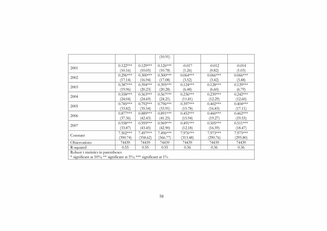
58

(10.91)

2001 0.122*** (10.16)

0.129*** (10.05)

0.126*** (10.78)

-0.017 (1.26)

-0.012 (0.82)

-0.014 (1.03)

2002 0.296*** (17.14)

0.300*** (16.94)

0.300*** (17.08)

0.064*** (3.52)

0.066*** (3.42)

0.066*** (3.48)

2003 0.387*** (19.96)

0.394*** (20.23)

0.395*** (20.28)

0.124*** (6.48)

0.128*** (6.60)

0.129*** (6.79)

2004 0.558*** (24.04)

0.563*** (24.69)

0.567*** (24.21)

0.236*** (11.81)

0.239*** (12.29)

0.242*** (12.60)

2005 0.785*** (33.82)

0.792*** (35.54)

0.796*** (33.91)

0.397*** (15.78)

0.402*** (16.83)

0.404*** (17.11)

2006 0.877*** (37.36)

0.889*** (42.43)

0.891*** (41.25)

0.452*** (15.94)

0.460*** (19.27)

0.462*** (19.55)

2007 0.938*** (33.87)

0.959*** (43.45)

0.969*** (42.90)

0.491*** (12.18)

0.505*** (16.59)

0.511*** (18.47)

Constant 7.502*** (390.74)

7.497*** (358.62)

7.496*** (366.77)

7.976*** (313.48)

7.973*** (290.76)

7.973*** (295.80)

Observations 74439 74439 74439 74439 74439 74439 R-squared 0.55 0.55 0.55 0.36 0.36 0.36 Robust t statistics in parentheses * significant at 10%; ** significant at 5%; *** significant at 1%

59

Table 16: Probit regressions of being poor with error terms adjusted for intragroup correlation (marginal effects). Dependent variable – binary variable for poverty. Equal to 1, if household’s income (consumption) is below poverty line. Access to finance is measured as the number of experts in a region

(1)

income poor

(2) income

poor

(3) income

poor

(4) consumption

poor

(5) consumption

poor

(6) consumption

poor Number of experts issued, lag1

-0.004** (2.49) -0.002

(0.61)

Number of experts issued, lag2 -0.007***

(2.74) -0.002 (0.43)

Number of experts issued, lag3 -0.013***

(3.71) -0.005 (1.01)

Number of nonperforming loans to performing, lag1

-1.919*** (4.08) -1.869*

(1.83)

Number of nonperforming loans to performing, lag2 -1.766***

(4.51) -1.593*** (2.63)

Number of nonperforming loans to performing, lag3 -0.220

(0.50) -0.495 (0.81)

Household size 0.092*** (14.53)

0.092*** (14.54)

0.092*** (14.50)

0.096*** (18.82)

0.096*** (18.91)

0.096*** (18.83)

Number of employed -0.150*** (14.80)

-0.150*** (14.82)

-0.150*** (14.83)

-0.084*** (13.83)

-0.085*** (13.81)

-0.085*** (13.77)

Number of children (0-14 years old)

0.032*** (5.29)

0.032*** (5.28)

0.032*** (5.28)

0.004 (0.90)

0.004 (0.88)

0.004 (0.88)

Number of elders (women older 55, men older 60)

-0.077*** (11.26)

-0.078*** (11.34)

-0.078*** (11.28)

-0.022*** (5.04)

-0.022*** (5.08)

-0.022*** (5.03)

Average years schooling -0.052*** (28.67)

-0.052*** (28.89)

-0.052*** (28.85)

-0.061*** (29.01)

-0.061*** (29.18)

-0.061*** (28.81)

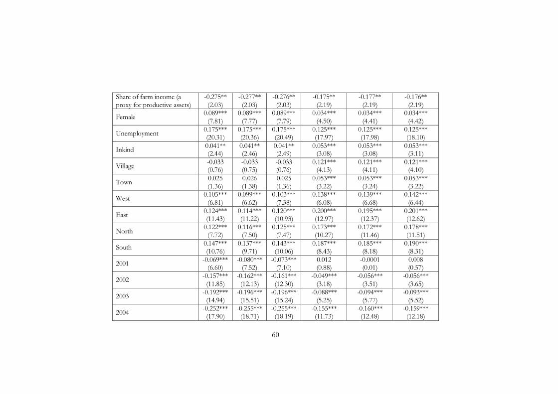
60

Share of farm income (a proxy for productive assets)

-0.275** (2.03)

-0.277** (2.03)

-0.276** (2.03)

-0.175** (2.19)

-0.177** (2.19)

-0.176** (2.19)

Female 0.089*** (7.81)

0.089*** (7.77)

0.089*** (7.79)

0.034*** (4.50)

0.034*** (4.41)

0.034*** (4.42)

Unemployment 0.175*** (20.31)

0.175*** (20.36)

0.175*** (20.49)

0.125*** (17.97)

0.125*** (17.98)

0.125*** (18.10)

Inkind 0.041** (2.44)

0.041** (2.46)

0.041** (2.49)

0.053*** (3.08)

0.053*** (3.08)

0.053*** (3.11)

Village -0.033 (0.76)

-0.033 (0.75)

-0.033 (0.76)

0.121*** (4.13)

0.121*** (4.11)

0.121*** (4.10)

Town 0.025 (1.36)

0.026 (1.38)

0.025 (1.36)

0.053*** (3.22)

0.053*** (3.24)

0.053*** (3.22)

West 0.105*** (6.81)

0.099*** (6.62)

0.103*** (7.38)

0.138*** (6.08)

0.139*** (6.68)

0.142*** (6.44)

East 0.124*** (11.43)

0.114*** (11.22)

0.120*** (10.93)

0.200*** (12.97)

0.195*** (12.37)

0.201*** (12.62)

North 0.122*** (7.72)

0.116*** (7.50)

0.125*** (7.47)

0.173*** (10.27)

0.172*** (11.46)

0.178*** (11.51)

South 0.147*** (10.76)

0.137*** (9.71)

0.143*** (10.06)

0.187*** (8.43)

0.185*** (8.18)

0.190*** (8.31)

2001 -0.069*** (6.60)

-0.080*** (7.52)

-0.073*** (7.10)

0.012 (0.88)

-0.0001 (0.01)

0.008 (0.57)

2002 -0.157*** (11.85)

-0.162*** (12.13)

-0.161*** (12.30)

-0.049*** (3.18)

-0.056*** (3.51)

-0.056*** (3.65)

2003 -0.192*** (14.94)

-0.196*** (15.51)

-0.196*** (15.24)

-0.088*** (5.25)

-0.094*** (5.77)

-0.093*** (5.52)

2004 -0.252*** (17.90)

-0.255*** (18.71)

-0.255*** (18.19)

-0.155*** (11.73)

-0.160*** (12.48)

-0.159*** (12.18)

61

2005 -0.302*** (22.00)

-0.305*** (22.47)

-0.305*** (22.35)

-0.221*** (13.53)

-0.228*** (14.14)

-0.226*** (14.43)

2006 -0.315*** (24.15)

-0.319*** (25.40)

-0.319*** (24.96)

-0.234*** (12.88)

-0.245*** (15.10)

-0.244*** (14.63)

2007 -0.322*** (22.85)

-0.327*** (25.21)

-0.329*** (25.17)

-0.248*** (10.80)

-0.259*** (14.25)

-0.262*** (14.85)

Observations 74439 74439 74439 74439 74439 74439 Robust z statistics in parentheses * significant at 10%; ** significant at 5%; *** significant at 1%

Table 17: Probit regression of being poor with error terms adjusted for intragroup correlation (marginal effects). Dependent variable – binary variable for poverty. Equal to 1, if household’s income (consumption) is below poverty line. Access to finance is measured as the number of loans issued in a region

(1)

income poor

(2) income

poor

(3) income

poor

(4) consumption

poor

(5) consumption

poor

(6) consumption

poor Number of loans issued, lag1

-0.005*** (2.58) -0.003

(0.93)

Number of loans issued, lag2 -0.006**

(2.08) -0.003 (0.68)

Number of loans issued, lag3 -0.009**

(2.38) -0.004 (0.75)

Number of nonperforming loans to performing, lag1

-1.894*** (3.95) -1.720

(1.61)

Number of nonperforming loans to -1.933***

(4.21) -1.518** (2.53)

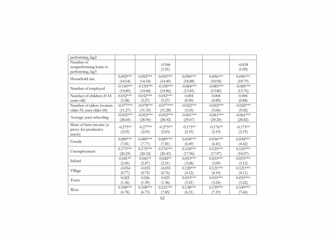
62

performing, lag2 Number of nonperforming loans to performing, lag3

-0.566 (1.01) -0.634

(1.00)

Household size 0.092*** (14.54)

0.092*** (14.54)

0.092*** (14.49)

0.096*** (18.88)

0.096*** (18.94)

0.096*** (18.79)

Number of employed -0.150*** (14.80)

-0.150*** (14.84)

-0.150*** (14.86)

-0.084*** (13.81)

-0.085*** (13.80)

-0.085*** (13.76)

Number of children (0-14 years old)

0.032*** (5.28)

0.032*** (5.27)

0.032*** (5.27)

0.004 (0.90)

0.004 (0.89)

0.004 (0.88)

Number of elders (women older 55, men older 60)

-0.077*** (11.27)

-0.078*** (11.33)

-0.077*** (11.28)

-0.022*** (5.03)

-0.022*** (5.06)

-0.022*** (5.02)

Average years schooling -0.052*** (28.69)

-0.052*** (28.90)

-0.052*** (28.92)

-0.061*** (29.07)

-0.061*** (29.20)

-0.061*** (28.82)

Share of farm income (a proxy for productive assets)

-0.275** (2.03)

-0.277** (2.03)

-0.275** (2.03)

-0.175** (2.19)

-0.176** (2.19)

-0.175** (2.19)

Female 0.089*** (7.81)

0.089*** (7.77)

0.089*** (7.81)

0.034*** (4.49)

0.034*** (4.41)

0.034*** (4.42)

Unemployment 0.175*** (20.25)

0.175*** (20.32)

0.176*** (20.43)

0.124*** (17.96)

0.125*** (17.97)

0.125*** (18.07)

Inkind 0.041** (2.45)

0.041** (2.47)

0.042** (2.51)

0.053*** (3.08)

0.053*** (3.09)

0.053*** (3.12)

Village -0.034 (0.77)

-0.033 (0.75)

-0.033 (0.76)

0.120*** (4.12)

0.121*** (4.10)

0.121*** (4.11)

Town 0.025 (1.36)

0.026 (1.39)

0.025 (1.36)

0.053*** (3.21)

0.053*** (3.24)

0.053*** (3.22)

West 0.108*** (6.78)

0.108*** (6.73)

0.121*** (7.85)

0.138*** (6.31)

0.139*** (7.19)

0.149*** (7.60)

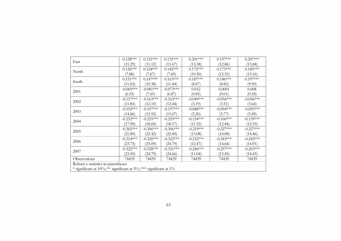
63

East 0.128*** (11.29)

0.121*** (11.12)

0.135*** (11.67)

0.201*** (13.38)

0.197*** (12.86)

0.207*** (13.68)

North 0.126*** (7.88)

0.124*** (7.67)

0.142*** (7.69)

0.172*** (10.50)

0.173*** (12.35)

0.185*** (13.16)

South 0.151*** (11.02)

0.147*** (10.38)

0.163*** (11.84)

0.187*** (8.67)

0.186*** (8.82)

0.197*** (9.90)

2001 -0.069*** (6.55)

-0.081*** (7.65)

-0.073*** (6.87)

0.012 (0.85)

0.0001 (0.01)

0.008 (0.58)

2002 -0.157*** (11.85)

-0.163*** (12.10)

-0.163*** (12.44)

-0.049*** (3.19)

-0.056*** (3.51)

-0.056*** (3.64)

2003 -0.192*** (14.86)

-0.197*** (15.55)

-0.197*** (15.07)

-0.088*** (5.20)

-0.094*** (5.77)

-0.093*** (5.49)

2004 -0.252*** (17.90)

-0.255*** (18.69)

-0.255*** (18.17)

-0.154*** (11.52)

-0.160*** (12.44)

-0.159*** (12.19)

2005 -0.302*** (21.89)

-0.306*** (22.42)

-0.306*** (22.00)

-0.219*** (13.08)

-0.227*** (14.08)

-0.227*** (14.46)

2006 -0.314*** (23.75)

-0.320*** (25.09)

-0.322*** (24.79)

-0.232*** (12.47)

-0.243*** (14.64)

-0.245*** (14.91)

2007 -0.322*** (23.50)

-0.328*** (24.79)

-0.331*** (24.66)

-0.246*** (11.04)

-0.257*** (13.45)

-0.263*** (14.43)

Observations 74439 74439 74439 74439 74439 74439 Robust z statistics in parentheses * significant at 10%; ** significant at 5%; *** significant at 1%

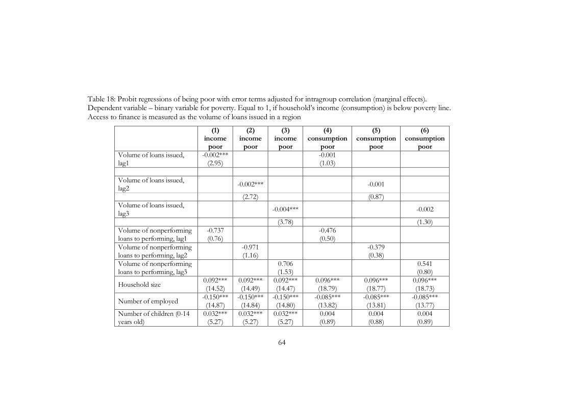
64

Table 18: Probit regressions of being poor with error terms adjusted for intragroup correlation (marginal effects). Dependent variable – binary variable for poverty. Equal to 1, if household’s income (consumption) is below poverty line. Access to finance is measured as the volume of loans issued in a region

(1)

income poor

(2) income

poor

(3) income

poor

(4) consumption

poor

(5) consumption

poor

(6) consumption

poor Volume of loans issued, lag1

-0.002*** (2.95) -0.001

(1.03)

Volume of loans issued, lag2 -0.002*** -0.001

(2.72) (0.87) Volume of loans issued, lag3 -0.004*** -0.002

(3.78) (1.30) Volume of nonperforming loans to performing, lag1

-0.737 (0.76) -0.476

(0.50)

Volume of nonperforming loans to performing, lag2 -0.971

(1.16) -0.379 (0.38)

Volume of nonperforming loans to performing, lag3 0.706

(1.53) 0.541 (0.80)

Household size 0.092*** (14.52)

0.092*** (14.49)

0.092*** (14.47)

0.096*** (18.79)

0.096*** (18.77)

0.096*** (18.73)

Number of employed -0.150*** (14.87)

-0.150*** (14.84)

-0.150*** (14.80)

-0.085*** (13.82)

-0.085*** (13.81)

-0.085*** (13.77)

Number of children (0-14 years old)

0.032*** (5.27)

0.032*** (5.27)

0.032*** (5.27)

0.004 (0.89)

0.004 (0.88)

0.004 (0.89)

65

Number of elders (women older 55, men older 60)

-0.078*** (11.29)

-0.078*** (11.31)

-0.078*** (11.26)

-0.022*** (5.02)

-0.022*** (5.03)

-0.022*** (5.01)

Average years of schooling -0.052*** (28.72)

-0.052*** (28.67)

-0.052*** (28.73)

-0.061*** (28.84)

-0.061*** (28.90)

-0.061*** (28.76)

Share of farm income (a proxy for productive assets)

-0.275** (2.03)

-0.276** (2.03)

-0.276** (2.03)

-0.175** (2.19)

-0.176** (2.19)

-0.176** (2.19)

Female 0.089*** (7.79)

0.089*** (7.77)

0.089*** (7.79)

0.034*** (4.41)

0.034*** (4.40)

0.034*** (4.41)

Unemployment 0.175*** (20.50)

0.175*** (20.39)

0.176*** (20.58)

0.125*** (18.27)

0.125*** (18.24)

0.125*** (18.37)

Inkind 0.041** (2.50)

0.041** (2.48)

0.041** (2.50)

0.053*** (3.12)

0.053*** (3.14)

0.053*** (3.15)

Village -0.034 (0.77)

-0.033 (0.75)

-0.033 (0.74)

0.120*** (4.11)

0.121*** (4.10)

0.121*** (4.11)

Town 0.025 (1.35)

0.026 (1.38)

0.026 (1.37)

0.053*** (3.19)

0.053*** (3.21)

0.053*** (3.21)

West 0.107*** (7.48)

0.103*** (7.48)

0.095*** (6.73)

0.144*** (6.14)

0.144*** (6.15)

0.140*** (5.66)

East 0.125*** (11.63)

0.118*** (10.44)

0.115*** (9.71)

0.204*** (11.99)

0.203*** (11.45)

0.202*** (11.16)

North 0.126*** (7.66)

0.121*** (7.77)

0.121*** (7.97)

0.180*** (10.52)

0.180*** (10.92)

0.181*** (11.03)

South 0.149*** (9.64)

0.141*** (8.84)

0.137*** (8.26)

0.193*** (8.79)

0.192*** (8.35)

0.190*** (7.98)

2001 -0.072*** (7.28)

-0.077*** (7.18)

-0.075*** (7.49)

0.007 (0.63)

0.004 (0.35)

0.005 (0.40)

2002 -0.160*** -0.162*** -0.162*** -0.054*** -0.056*** -0.056***

66

(12.48) (12.41) (12.43) (3.69) (3.62) (3.65)

2003 -0.194*** (15.54)

-0.197*** (15.63)

-0.197*** (15.62)

-0.092*** (5.62)

-0.094*** (5.88)

-0.096*** (5.96)

2004 -0.253*** (18.28)

-0.254*** (18.73)

-0.255*** (18.56)

-0.157*** (11.96)

-0.159*** (12.65)

-0.161*** (13.00)

2005 -0.304*** (22.18)

-0.305*** (22.97)

-0.305*** (22.55)

-0.225*** (13.67)

-0.227*** (14.40)

-0.228*** (14.74)

2006 -0.318*** (24.42)

-0.320*** (26.20)

-0.320*** (25.81)

-0.242*** (13.39)

-0.245*** (15.33)

-0.246*** (15.52)

2007 -0.325*** (21.95)

-0.329*** (25.83)

-0.330*** (26.28)

-0.257*** (11.24)

-0.262*** (14.30)

-0.264*** (16.05)

Observations 74439 74439 74439 74439 74439 74439 Robust z statistics in parentheses * significant at 10%; ** significant at 5%; *** significant at 1%

67

Table 19: Quantile regression. Dependent variable – ln of income. Access to finance indicator is measured as the number of loans issued in a region with three lags

0.1 percentile

0.25 percentile

0.5 percentile

0.75 percentile

0.9 percentile

Number of loans issued, lag3

0.004** (2.22)

0.004*** (3.04)

0.006*** (4.40)

0.010*** (6.65)

0.011*** (5.50)

Number of nonperforming loans to performing, lag3

1.435*** (3.92)

1.286*** (4.43)

1.460*** (4.71)

0.838** (2.42)

1.140** (2.49)

Household size -0.136*** (45.44)

-0.139*** (61.66)

-0.138*** (57.70)

-0.139*** (49.81)

-0.141*** (36.37)

Number of employed 0.232*** (64.54)

0.231*** (85.50)

0.224*** (79.37)

0.204*** (63.68)

0.184*** (42.97)

Number of children (0-14 years old)

-0.041*** (9.15)

-0.033*** (9.68)

-0.024*** (6.46)

-0.009** (2.25)

0.008 (1.45)

Number of elders (women older 55, men older 60)

0.190*** (57.50)

0.141*** (55.75)

0.090*** (33.21)

0.045*** (14.15)

0.007* (1.71)

Average years schooling 0.049*** (31.77)

0.054*** (44.91)

0.064*** (49.79)

0.075*** (52.26)

0.088*** (46.29)

Share of farm income (a proxy for productive assets)

0.469*** (21.17)

0.564*** (49.30)

0.611*** (66.26)

0.613*** (66.89)

0.539*** (44.39)

Female -0.083*** (15.20)

-0.107*** (25.76)

-0.126*** (28.82)

-0.140*** (28.15)

-0.136*** (20.26)

Unemployment -0.253*** (45.30)

-0.217*** (50.67)

-0.186*** (41.76)

-0.163*** (32.98)

-0.148*** (22.74)

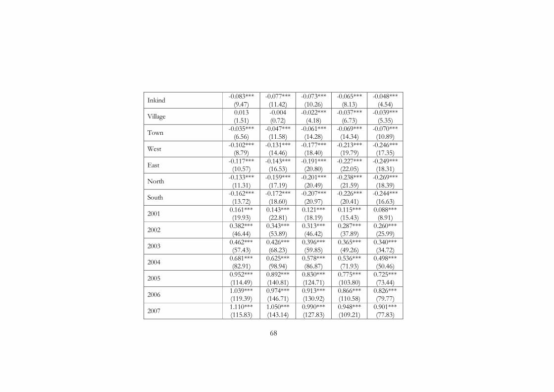
68

Inkind -0.083*** (9.47)

-0.077*** (11.42)

-0.073*** (10.26)

-0.065*** (8.13)

-0.048*** (4.54)

Village 0.013 (1.51)

-0.004 (0.72)

-0.022*** (4.18)

-0.037*** (6.73)

-0.039*** (5.35)

Town -0.035*** (6.56)

-0.047*** (11.58)

-0.061*** (14.28)

-0.069*** (14.34)

-0.070*** (10.89)

West -0.102*** (8.79)

-0.131*** (14.46)

-0.177*** (18.40)

-0.213*** (19.79)

-0.246*** (17.35)

East -0.117*** (10.57)

-0.143*** (16.53)

-0.191*** (20.80)

-0.227*** (22.05)

-0.249*** (18.31)

North -0.133*** (11.31)

-0.159*** (17.19)

-0.201*** (20.49)

-0.238*** (21.59)

-0.269*** (18.39)

South -0.162*** (13.72)

-0.172*** (18.60)

-0.207*** (20.97)

-0.226*** (20.41)

-0.244*** (16.63)

2001 0.161*** (19.93)

0.143*** (22.81)

0.121*** (18.19)

0.115*** (15.43)

0.088*** (8.91)

2002 0.382*** (46.44)

0.343*** (53.89)

0.313*** (46.42)

0.287*** (37.89)

0.260*** (25.99)

2003 0.462*** (57.43)

0.426*** (68.23)

0.396*** (59.85)

0.365*** (49.26)

0.340*** (34.72)

2004 0.681*** (82.91)

0.625*** (98.94)

0.578*** (86.87)

0.536*** (71.93)

0.498*** (50.46)

2005 0.952*** (114.49)

0.892*** (140.81)

0.830*** (124.71)

0.775*** (103.80)

0.725*** (73.44)

2006 1.039*** (119.39)

0.974*** (146.71)

0.913*** (130.92)

0.866*** (110.58)

0.826*** (79.77)

2007 1.110*** (115.83)

1.050*** (143.14)

0.990*** (127.83)

0.948*** (109.21)

0.901*** (77.83)

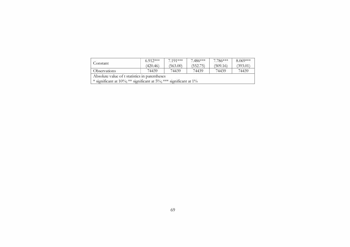
69

Constant 6.912*** (420.46)

7.191*** (563.00)

7.486*** (552.75)

7.786*** (509.16)

8.069*** (393.01)

Observations 74439 74439 74439 74439 74439 Absolute value of t statistics in parentheses * significant at 10%; ** significant at 5%; *** significant at 1%

70

BIBLIOGRAPHY

Aghion, Phillipe, and Patrick Bolton. "A theory of trickle-down growht and development ." The Review of Economic Studies , 1997: 151-172.

Andersen, Susan R. The influence and effects of financial development on economic growth. Bergen: Chr. Michelsen Institute, 2003.

Aportela, Francisco. Effects of financial access on savings by low-icome people. Cambridge, MA: MIT, 1999.

Appleton, Simon. "'The rich are just like us only richer': poverty functions or consumption functions." Journal of African Economies, 2002: 433-469.

Arnall, Dawn. Microfinance in the US. 11 26, 2006. http://thehague.usembassy.gov/mrs._arnall_microfinance/ (accessed 12 11, 2008).

Ashe, Jeffrey. "Microfinance in the United States: the Working Capital experience - ten years of lending and learning." Journal of Microfinance, 2000: 22-60.

Ashenfelter, O., and A. Krueger. "Estimates of the economic return to schooling from a new sample of twins." American Economic Review, 1992: 1157–74.

Ashraf, Nava, Xavier Gine, and Dean Karlan. Finding missing markets: an evaluation of a horticultural export and credit program in Kenya. Washington, DC: World Bank, 2007.

Atkinson, A., L. Rainwater, and T. Smeedin. Income distribution in advanced economies: evidence from Luxembourge income study. Luxembourge: Luxembourge Income Study Working Paper #12, 1995.

Atkinson, Anthony B. "Comparing Poverty Rates Internationally: Lessons from Recent Studies in Developed Countries." World Bank Economic Review, 1991: 3-21.

Baldwin, Majorie, and William G. Johnson. "Labor market discrimination against women with disabilities." Journal of Human Resources, 1994: 1-19.

Banerjee, Abhijit V., and Andrew F. Newman. "Occupatinal choice and the process of development." Journal of Political Economy, 1993: 274-298.

Baulch, Bob, and Edoardo Masset. "Do monetary and nonmonetary indicators tell the same story about chronic poverty? A study of Vietnam in the 1990s." World Development, 2003: 441-453.

71

Beck, Thorsten, Asli Demirguc-Kunt, and Maria Soledad Martinez Peria. "Reaching out: access to and use of banking servieses accross countries." Journal of Financial Economics, 2007: 234-266.

Beck, Thorsten, Asli Demirguc-Kunt, and Ross Levine. "Finance, inequality and the poor." Journal of Economic Growth, 2007: 27-49.

Becker, Gary S., and Barry R. Chiswick. "Education and the distribution of earnings." American Economic Review, 1966: 358-69.

Bena, Jen, and Stepan Jurajda. Which firms benefit more from financial development . Prague: CERGE-EI, 2007.

Bernanke, Ben S. "Microfinance in the United States." Board of Governors of the Federal Reserve System. 11 06, 2006. http://www.federalreserve.gov/newsevents/speech/bernanke20071106a.htm (accessed 12 11, 2008).

Besley, Timothy, and Stephen Coate. "Group lending, repayment incentives and social collateral." Journal of Development Economics, 1995: 1-18.

Bhatt, Nitin, and Shui-Yan Tang. "Determinants of repayment in microcredit: evidence from programs

in the United States ." International Journal of Urban and Regional Research, 2002: 360-376.

Bokosi, Fanwell K. "Household poverty dynamics in Malawi: a bivariate probit analysis." Journal of Applied Sciences, 2007: 258-262.

Bruck, Tirman, M. Alexander Danzer, Alexander Muravyav, and Natalia Weibhar. Determinants of poverty during transition: household survey evidence from Ukraine. PRUS, 2007.

Burgess, Robin, and Rohini Pande. "Do rural banks matter? Evidence from the Indian Social Banking Experiment." The American Economic Review, 2005: 780-795.

Burgess, Robin, and Rohini Pande. Do rural banks matter? Evidence from the Indian Social Banking Experiment. Bureau for research in economic analysis of development, 2003.

Clark, Peggy, and Amy Kay. Microenterprise and the poor: findings from the self-employment learning project. Washington, DC: The Aspen Institute, 1999.

Clarke, George R. G., Lixin Colin Xu, and Heng-fu Zou. "Finance and income inequality: what do the data tell us?" Southern Economic Journal, 2006: 578–596.

72

Coudouel, A., Jesko S. Hentschel, and Quentin. T. Wodon. Poverty Measurement and Analysis. Washington, D.C.: World Bank, 2002.

Cull, Robert, Asli Demirguc-Kunt, and Jonathan Morduch. "Financial performance and outreach: a global analysis of leading microbanks." Economic Journal, 2007: F107-F133.

Datt, G., K. Simler, S. Mukherjee, and G. Dava. Determinants of poverty in Mozambique: 1996-97. FCND DISCUSSION PAPER, Washington, D.C.: International Food Policy Research Institute, 2000.

Datt, Gaurav, and Dean Jolliffe. Determinants of poverty in Egypt: 1997. FCND DISCUSSION PAPER, Washington, D.C.: International Food Policy Research Institute, 1999.

de Avila, Diego R. Finance and growth in the EU: new evidence from the liberalization and harmonization of the banking industry. Frankfurt: European Central Bank, 2003.

De Janvry, Alain, Craig McIntosh, and Elisabeth Sadoulet. The supply and demand side impacts of credit market information. Berkeley, CA: University of California, Berkeley, Agricultural and Resource Economics, 2006.

de Vos, Klaas, and Asghar M. Zaidi. "Equivalence Scale Sensitivity of

Poverty Statistics for the Member States of the European Community." Review of Income and Wealth, 1997: 319-333.

Demirguc-Kunt, Asli, Thorsten Beck, and Patrick Honohan. Finance for all?: policies and pitfalls in expanding access. A World Bank policy research report, Washington D.C.: World Bank, 2007.

Ehrenberg, Ronald G., and Robert S. Smith. Modern labor economics: theory and public policy. The Addison-Wesley Longman, Inc., 2000.

Finnie, R., and A. Sweetman. "Poverty Dynamics: Empirical Evidence for Canada." The Canadian Journal of Economics, 2003: 291-325.

Ghatak, Maitreesh, and Timothy W. Guinnane. "The economics of lending with joint liability: theory and practice." Journal of Development Economics (Economic Growth Center, Yale University), 1999: 195-228.

Gine, Xavier, and Robert M. Townsend. Evaluatin of financial liberalization: a general equilibrium model with constrained occupation choice. Washington D.C.: World Bank, 2004.

Gine, Xavier, Pamela Jakiela, Dean Karlan, and Jonathan Morduch. Microfinance games. Washington, DC: World Bank, 2006.

73

Goldberg, Nathanael. "Measuring the impact of microfinance: taking stock of what we know." Grameen Foundation. December 2005. http://www.grameenfoundation.org/pubdownload/~pubid=29 (accessed November 14, 2008).

Gorodnichenko, Yuriy, and Klara Sabirianova Peter. "Returns to schooling in Russia and Ukraine: a semiparametric approach to cross-country comparative analysis ." Journal of Comparative Economics, 2005: 324-350.

Grootaert, Christiaan. "The determinants of poverty in Cote d'Ivoire in the 1980s." Journal of African Economies, 1997: 169-196.

Heckman, J. James, J. Lanc Lochner, and E. Todd Petra. Fifty years of Mincer earnings regressions. National Bureau of Economic Research, 2003.

Himes, Christina, and Lisa J. Servon. Measuring Client Success: An Evaluation of Accion’s Impact on Microenterprises in the United States. Boston: Accion International, 1998.

Jacoby, Hanan G. "Borrowing constraints and progress through school: Evidence from Peru." Review of Economics and Statistics, 1994: 151-160.

Karlan, Dean S. "Social connections and group banking." Economic Journal, 2007: F52-F84.

Karlan, Dean, and Jonathan Zinman. Observing unobservables: identifying information asymmetries with a consumer credit field experiment. New Haven, CT: Yale University, Department of Economics, 2006.

King, Robert G., and Ross Levine. "Finance and growth: Schumpeter might be right." The Quartely Journel of Economics, 1993: 717-737.

Kislitsyna, Olga. Income Inequality in Russia during Transition: How Can It Be Explained? Working Paper, Moscow: EERC, 2003.

Koenker, Roger, and Kevin F. Hallock. "Quantile regression." Journal of Economic Perspectives, 2001: 143–156.

Koo, Jaewoon, and Kyunghee Maeng. "The effect of financial liberalization on firms' investments in Korea." Journal of Asian Economics, 2005: 281-297.

Kreuz, Claudia. Microlending in Germany. Geneva: International Labour Organisation, 2006.

Levine, Ross. "Financial development and economic growth:

74

views and agenda." Journal of Economic Literature, 1997: 688–726.

Levine, Ross. More on finance and growth: more finance, more growth? . St. Louis: The Federal Reserve Bank of St. Louis, 2003.

Li, Hongyi, Lyn Squire, and Heng-fu Zou. "Explaining international and intertemporal variations in income inequality." The Economic Journal, 2001: 26-43.

Love, Inessa, and Lea Zicchino. Financial development and dynamic investment behavior: evidence from panel vector autoregression. Washington D.C.: World Bank, 2004.

Macho-Stadler, Ines, and J. David Perez-Castrillo. An introduction to the economics of information. New York: Oxford University Press Inc., 2001.

Mahjabeen, Rubana. "Microfinancing in Bangladesh: impact on households, consumption and welfare." Journal of Policy Modeling, 2008: 1083–1092.

Milanovic, Branko. "Income, inequality and poverty in the transition: A survey of the evidence." MOCT-MOST: Economic Policy in Transitional Economies, 2006: 131-147.

Morduch, Jonathan. "The Microfinance Promise." Journal of Economic Literature, 1999: 1569–1614.

Moulton, B. R. "An illustration of a pitfall in estimating the effects of aggregate variables on micro units." The Review of Economics and Statistics, 1990: 334-338.

Moulton, B. R. "Random group effects and the precision of regression estimates." Journal of Econometrics, 1986: 385-397.

OECD Social Policy Division. "What are equivalence scales?" Organization of Economic Cooperation and Development. n.d. www.oecd.org/dataoecd/61/52/35411111.pdf (accessed May 20, 2009).

Ravallion, Martin. Poverty comparisons: a guide to concepts and methods. Washington DC: World Bank, 1992.

Schreiner, Mark. "Self-employment, microenterprise, and the poorest." Social Service Review, 1999: 496-523.

Schreiner, Mark, and Jonathan Morduch. Replicating microfinance in the United States: opportunities and challenges. Washington, DC: Fannie Mae Foundation, 2001.

Schumpeter, Joseph A. The Theory of Economic Development. Cambridge: Harvard University Press, 1911.

75

Temple, Jonathan. "The new growth evidence." Journal of Economic Literature, 1999: 112-156.

The World Bank. Ukraine: Poverty Update. Report No. 39887, Washington D.C.: The World Bank, 2007.

Valdivia, Martin, and Dean Karlan. Teaching entrepreneurship: impact of business training on microfinance clients and institutions. New Heaven, CT: Economic Growth Center, Yale University, 2006.

Zeller, Manfred. "Conference on social protection and poverty." The role of micro-finance for income and consumption smoothing. Washington D.C.: Inter-American Development Bank, 1999. 1-26.

Державний Комітет Статистики України. "Наказ №223 "Про затвердження методологічних основ формування вибіркових сукупностей для проведення органами державної статистики України базових державних обстежень населення (домогосподарств)"." zakon.nau.ua. August 2, 2005. http://zakon.nau.ua/doc/?uid=1041.30590.1&nobreak=1 (accessed March 20, 2009).

Кабінет Міністрів України. "Постанова №1725 "Про

проведення обстеження умов життя у домогосподарствах"." zakon.rada.gov.ua. March 2, 1998. http://zakon.rada.gov.ua/cgi-bin/laws/main.cgi?nreg=1725-98-%EF (accessed March 20, 2009).

Міністерство праці та соціальної політики України, Міністерство фінансів України, Міністерство економіки та з питань європейської інтеграції, Державний комітет статистики України, Національна академія наук України. "Наказ №171/238/100/149/2нд "Про затвердження методики комплексної оцінки бідності"." zakon.nau.ua. April 5, 2002. http://zakon.nau.ua/doc/?uid=1029.365.0 (accessed April 10, 2009).

76