the influence of ply orientation on the open … · tension strength of composite laminates . by ....
TRANSCRIPT

THE INFLUENCE OF PLY ORIENTATION ON THE OPEN-HOLE
TENSION STRENGTH OF COMPOSITE LAMINATES
By
DANIEL PAUL STONE
A thesis submitted in partial fulfillment of the requirements for the degree of
MASTER OF SCIENCE IN MECHANICAL ENGINEERING
WASHINGTON STATE UNIVERSITY Department of Mechanical and Materials Engineering
MAY 2008

To the Faculty of Washington State University:
The members of the Committee appointed to examine the thesis of DANIEL PAUL STONE find it satisfactory and recommend that it be accepted.
___________________________________ Chair ___________________________________ ___________________________________
ii

ACKNOWLEDGMENT
This project would not have been possible without the insightful guidance of Dr.
Lloyd V. Smith, whose advice and knowledge were irreplaceable. I’d also like to thank
my committee members, Dr. Jow-Lian Ding and Dr. Vikram Yadama, for their help and
expertise, and to Dr. Kip Findley, for his instruction while he was at WSU. I’d also like
to thank Arjun Kothidar, my partner in this project, for all the work and discussion that he
has contributed. Boeing funded the initial part of this research, and their financial support
is appreciated.
As any researcher knows, work does not get done without the help of the machine
shop. Thanks to Kurt Hutchison, Jon Grimes, Norm Martel, and Henry Ruff for their help
with various aspects of composite fabrication. A special thanks to Steve Myers and
Myers Auto Rebuild and Towing for their patience and professionalism while
discovering how to best speckle the composites. Thank you to the MME staff, including
Jan Danforth, Bob Ames, Gayle Landeen, and Annette Cavalieri, who were always
reliable and whose sociability made my life better. I’d also like to thank Giac Pham and
Micheal Shook for their help and competence with technical issues. Thank you to all the
WSU researchers who have helped me throughout this project, including Matt Shultz,
Matthew Jorgensen, Alex Butterfield, and Tyler Start.
Lastly, and most importantly, I would like to thank my family for their
encouragement throughout my years of learning. To my parents, David and JoAnne
Stone, and to my brother, Jamie Stone, thank you, I could not have graduated without
your love, guidance, and support.
iii
THE INFLUENCE OF PLY ORIENTATION ON THE OPEN-HOLE
TENSION STRENGTH OF COMPOSITE LAMINATES
Abstract
by Daniel Paul Stone, M.S.
Washington State University May 2008
Chair: Lloyd V. Smith
Composite laminates can be tailored for a specific loading scenario by varying the ply
orientation. In open-hole tension, a circular area is removed from the center of the
composite specimen to simulate the stress concentration that occurs during the
introduction of a bolt or rivet. This stress concentration leads to a decrease in the strength
of the specimen, and is likely to be the location of crack initiation in an engineering
structure. Increases in first ply failure and ultimate tensile strength have been found by
tailoring the ply orientation for open-hole tension.
The strain fields of the tailored laminates have been characterized using the digital
image correlation method (DICM), Moiré interferometry (MI), and finite element
analysis (FEA). Results indicate that DICM is a useful tool for measuring the first ply
failure of the laminate. DICM accurately characterized the strain around the hole
throughout damage progression, and was verified using MI and FEA.
The failure criteria examined in the current study include Maximum Strain,
Maximum Stress, Tsai-Wu, Tsai-Hill, Hoffman, Hashin, and Yamada-Sun. The first ply
failure predictions of these criteria were compared to those experimentally measured by
DICM. The Maximum Strain and Maximum Stress failure criteria most accurately
predicted first ply failure.
iv

Eight non-traditional laminates were optimized to reduce the stress concentration and
increase the first ply failure. The influence of the ply orientation on the open-hole tension
strength of these laminates was examined. Significant increases in strength were found by
varying the ply orientation of the secondary load bearing plies (±45º and 90º), with
relatively small material property trade-off for some laminates. Thus, improvements in
strength were found for the tailored laminates in the open-hole tension loading scenario.
v

TABLE OF CONTENTS Page ACKNOWLEDGEMENT ...................................................................................................iii
ABSTRACT ......................................................................................................................... iv
LIST OF TABLES ............................................................................................................... ix
LIST OF FIGURES .............................................................................................................. x
CHAPTER
1 LITERATURE REVIEW ...................................................................................... 1
1.1 Introduction ............................................................................................. 1
1.2 Laminate Stacking Sequence .................................................................. 3
1.3 Layup ...................................................................................................... 5
1.4 Ply Orientation ........................................................................................ 8
1.5 Failure Criteria ...................................................................................... 11
1.5.1 Mode-based Failure Criteria .............................................................. 12
1.5.2 Quadratic Interaction Failure Criteria ................................................ 14
1.5.3 Failure Criteria versus Experimental Results .................................... 15
1.6 Failure Progression ............................................................................... 19
1.7 Conclusion ............................................................................................ 20
2 FINITE ELEMENT ANALYSIS ........................................................................ 22
2.1 Finite Element Model ........................................................................... 22
2.2 Optimization Methods .......................................................................... 27
2.3 Model Verification ................................................................................ 29
2.4 FEA Results .......................................................................................... 31
vi
3 DIGITAL IMAGE CORRELATION METHOD ................................................ 37
3.1 Experimental Technique ....................................................................... 37
3.2 Moiré Interferometry ............................................................................ 44
4 MANUFACTURING .......................................................................................... 48
4.1 Prepreg .................................................................................................. 48
4.2 Fabrication ............................................................................................ 48
5 RESULTS ............................................................................................................ 50
5.1 Introduction ........................................................................................... 50
5.2 Strain Profile ......................................................................................... 53
5.3 Failure Modes ....................................................................................... 68
5.4 Experimental and Theoretical FPF for Non-Traditional Laminates ..... 77
5.5 Strength ................................................................................................. 82
6 CONCLUSION .................................................................................................... 88
REFERENCES ................................................................................................................... 91
APPENDIX
A. TABLES ........................................................................................................... 95
B. COUPON DIMENSIONS ................................................................................ 96
C. CONVERGENCE STUDY FOR LOCATIONS (X,Y).................................... 97
D. OPTIMIZATION USING FEA ........................................................................ 98
D.1 Decrease the strain concentration, kt .................................................... 98
D.2 Increase the first ply failure, FPF ......................................................... 99
D.3 Example of a double angle optimization ............................................ 100
E. MATLAB PROGRAM FOR FAILURE CRITERIA ...................................... 101
vii

F. SELECTED STRAIN CONTOURS ................................................................ 105
H. PROPORTIONAL LIMIT COMPARED TO MAXIMUM STRAIN FPF ..... 110
H.1 Applied stress vs. longitudinal strain ................................................. 110
H.2 Applied stress vs. shear strain ............................................................ 113
I. SELECTED LAMINATES AT OR NEAR FAILURE .................................... 116
viii
LIST OF TABLES
2.1.1 T600: 125-33 Composite Material System (psi) ........................................................ 24
2.4.1 Method 1: reduce kt .................................................................................................... 34
2.4.2 Method 2: increase FPF ............................................................................................. 34
2.4.3 Fabricated layups ....................................................................................................... 35
5.1.1 Fabricated layups ....................................................................................................... 50
5.4.1 Failure Modes for FPF as predicted by Maximum Strain Criterion .......................... 78
5.4.2 Number of DICM coupons experimentally tested for Fig. 5.4.5 ............................... 82
5.5.1 Number of DICM coupons experimentally tested for Fig. 5.5.1 ............................... 84
5.5.2 Number of DICM coupons experimentally tested for Fig. 5.5.2 ............................... 86
ix

LIST OF FIGURES
1.1.1 Definition of fiber angle in a composite laminate under tensile stress [3] ................. 2 1.3.1 Joint configuration (dimensions in mm) [10] ............................................................. 6 1.5.1 Comparison between the predicted and measured failure stresses for a unidirectional fibre-reinforced lamina made of GRP material E-Glass/Ly556/HT907/ Dy063 and subjected to combined shear and normal stresses perpendicular to the fibres (Test Case no. 1). [1] .......................................................................................................... 17 1.5.2 Comparison between the predicted and measured biaxial failure envelope for a unidirectional fibre-reinforced GRP lamina under combined normal stresses in directins parallel (σx) and perpendicular (σy) to the fibres. Material: E-glass/MY750 epoxy (Test Case No. 3). [1] .................................................................................................................. 17 1.5.3 (a) Comparison between the predicted and measured final failure stresses for (±55º) E-glass/MY750 laminates subjected to biaxial loads (Test Case No. 9). (b) Comparison between the predicted and measured ‘initial’ failure stresses for (±55º) E-glass/MY750 laminates subjected to biaxial loads (Test Case No. 9). [1] ............................................... 18 1.6.1 Failure mechanisms for laminates loaded in tension [2] .......................................... 19 2.1.1 2D Finite Element Model ........................................................................................... 22 2.1.2 Boundary Conditions ................................................................................................. 23 2.1.3 Shell99 Element (© Ansys 2006) ............................................................................. 23 2.1.4 Ply orientations in Ansys ........................................................................................... 26 2.1.5 Final Mesh ................................................................................................................. 27 2.2.1 Strain Concentration .................................................................................................. 28 2.3.1 kt versus the hole-to-width ratio (d/D) for an isotropic material ............................... 30 2.3.2 Longitudinal strain vs. distance along X and Y ......................................................... 31 2.4.1 kt vs. the percentage of 45º plies for the baseline layup ............................................ 32 2.4.2 FEA Coordinates and locations of interest ................................................................ 33 2.4.3 Material properties from CLT of non-traditional laminates normalized to the baseline (BL) layup ............................................................................................................. 36
x
3.1.1 Longitudinal strain (tensile loading is horizontal) ..................................................... 37 3.1.2 Speckle pattern ........................................................................................................... 38 3.1.3 Image correlation [43]................................................................................................ 40 3.1.4 Image correlation showing a.) the reference image b.) the deformed image and c.) the subset matching [43] ..................................................................................................... 40 3.1.5 Speckle patterns for Layup B showing a.) a mediocre pattern (coupon1), b.) a better pattern (coupon 2), and c.) a good pattern (coupon 3) ........................................................ 43 3.1.6 Strain profiles for Layup B for a.) coupon 1, b.) coupon 2, and c.) coupon 3, corresponding to the speckle patterns of Fig. 3.1.5a-c and showing improved correlation for speckle patterns that are isotropic, high contrast, and with smaller areas of black and white .................................................................................................................................... 43 3.1.7 DICM parameter study for a.) Subset, and b.) Step Size ........................................... 44 3.2.1 Moiré Interferometry fringe pattern [55] ................................................................... 45 3.2.2 Moiré Interferometry measurement technique [56] ................................................... 45 4.2.1 Fabrication setup ........................................................................................................ 49 5.1.1 a.) Von Mises strain map measured by DICM around a 5 mm hole on a thermoplastic matrix composite, σapplied=67% σfailure (vertical loading) [45] b.) Transverse displacement (mm x 10-3) contour plots by DICM near a bolt (vertical load) [52] ............ 51 5.1.2 Longitudinal strain versus distance from the hole at the net section of a fatigued [0/±45/90]2s graphite/PEEk sample; maximum load=75% of the ultimate static load [46] ...................................................................................................................................... 51 5.1.3 Idealized load-strain curve for uniaxially loaded laminate showing multiple ply failures leading up to ultimate laminate failure. [26] .......................................................... 52 5.1.4 Comparison of predicted and measured stress-strain response of [0/±45/90]s glass/epoxy laminate. [53] .................................................................................................. 52 5.2.1 a.) Longitudinal strain DICM contours and b.) Principle strain vectors for the Baseline laminate at 19 Ksi (26% UTS), where tensile loading is horizontal .................... 54 5.2.2 Moiré Interferometry longitudinal deformation contour for the baseline layup at 19 Ksi (26% UTS), where tensile loading is horizontal .......................................................... 55
xi

5.2.3 Strain contours for layup A at 38 Ksi (53% UTS) in a strain range of 0.00117 in/in to 0.0121 in/in for a.) DICM and b.) 2D linear FEA. The gray band for b.) near the top and side of the hole represents strains above and below the strain range ........................... 56 5.2.4 Strain vs. Y distance from the hole using DICM for a.) longitudinal strain: layup D, b.) shear strain: layup B, and c.) transverse strain: layup A ............................................... 57 5.2.5 Strain vs. Y distance from the hole plots of selected coupons at 90% UTS for a.) longitudinal strain and b.) shear strain ................................................................................ 58 5.2.6 Stress vs. strain plots of selected coupons for a.) longitudinal strain and b.) shear strain .................................................................................................................................... 59 5.2.7 Longitudinal strain of layup A as a function of distance from the hole for DICM and 2D FEA ............................................................................................................................... 60 5.2.8 Longitudinal strain contours for layup A at a.) 90% UTS and b.) 98% UTS showing the maximum strain at the left of the net-section during high damage ............................... 60 5.2.9 a.) Diagram showing the crack and the location of the strain profiles, and b.) strain profiles for Layup A at 90% UTS ....................................................................................... 61 5.2.10 Longitudinal strain vs. distance from the hole for DICM and 2D FEA at 90% UTS for a.) Layup A, b.) Layup B, c.) Layup C, and d.) Layup D ............................................. 62 5.2.11 Longitudinal strain vs. distance from the hole for DICM and 2D FEA at 25% UTS for a.) Layup A, b.) Layup B, c.) Layup C, and d.) Layup D ............................................. 63 5.2.12 Strain profile for Layup A showing experimental variation at 25% UTS for a.) coupon 1, and b.) coupon 2 ................................................................................................. 63 5.2.13 Strain Profiles at the top and bottom of the hole along the net section for Layup G at a.) 24% UTS, and b.) 89% UTS ...................................................................................... 64 5.2.14 Longitudinal strain vs. distance from the hole at 19 Ksi (25% UTS) for Layup B using Moiré Interferometry, DICM, and FEA .................................................................... 64 5.2.15 Comparison of experimental (DICM) and theoretical (2D linear FEA) results for the strain concentration, kt, at the DICM location (εmax at 0.022 inches from the hole and εmin at (0.5, 0.375) inches from the coupon center) ............................................................ 66 5.2.16 Comparison of the kt from the DICM location (εmax at 0.022 inches from the hole and εmin at (0.5, 0.375) inches from the coupon center) to the kt from Location A (εmax at Location A, Fig. 2.4.1, and εmin at (4, 0) from the coupon center ) .................................... 66
xii

5.2.17 Comparison of experimental (DICM) and theoretical (FEA) results for the longitudinal modulus, Ex ..................................................................................................... 67 5.3.1 Stress vs. longitudinal strain for a uniaxial coupon (Layup J) showing an increase in stiffness after damage initation (at Location A, Fig. 2.4.1) ................................................ 69 5.3.2 Maximum vs. nominal strain for layup J (uniaxial), indicating a stress redistribution where the slope (representing the strain concentration) decreases, corresponding to an increase in stiffness in Fig.5.3.1 (at Location A, Fig 2.4.1) ................................................ 69 5.3.3 Strain contours at 90% UTS for a.) longitudinal strain, b.) transverse strain and, c.) shear strain. Image “d” shows the uniaxial coupon failed due to matrix splitting at the sides of the hole .................................................................................................................. 71 5.3.4 DICM (left image) and FEA (right image) strain contours at 25% UTS for a.) longitudinal strain, b.) transverse strain, and c.) shear strain .............................................. 72 5.3.5 Stress-strain plots for a.) shear, b.) transverse, and c.) axial strain at Location B of the uniaxial “J” laminate showing FPF and SPF ................................................................ 74 5.3.6 Stress-strain plots of the ±45 failure-mode layup I for a.) longitudinal strain and b.) shear strain comparing the proportional limit to the FPF predicted by the Maximum Strain Criterion.................................................................................................................... 76 5.3.7 Experimental FPF using DICM and the proportional compared to FPF predicted by common failure criteria ....................................................................................................... 77 5.4.1 Stress vs. longitudinal strain for locations from the hole along Y (Fig. 2.4.1) for Layup D .............................................................................................................................. 79 5.4.2 Stress vs. longitudinal strain for loading and reloading up to 90% UTS, compared to Maximum Strain predicted FPF (Layup D) ........................................................................ 79 5.4.3 Stress vs. longitudinal strain showing the proportional limit compared to Maximum Strain predicted FPF (layup F) ............................................................................................ 80 5.4.4 Stress vs. longitudinal strain for layup B, comparing the proportional limit to Maximum Strain predicted FPF .......................................................................................... 81 5.4.5 Experimental FPF (proportional limit, DICM) for non-traditional laminates, compared to common failure criteria .................................................................................. 82 5.5.1 Experimental first ply failure for non-traditional layups using DICM and the proportional limit ................................................................................................................ 84 5.5.2 Experimental ultimate tensile stress for non-traditional layups ................................. 86
xiii

xiv
5.5.3 Material properties of non-traditional laminates normalized to the baseline (BL) layup .................................................................................................................................... 87
1: Literature Review
1.1: Introduction
The operating strain level in engineering structures is often restricted by the presence
of bolts or rivets. The hole drilled for such a fastener introduces a stress concentration
that increases stress by a factor of three in an ideal material. While this effect may be
reduced in metal structures by cold working holes, the same is not possible for carbon
fiber reinforced plastics (CFRP) due to negligible plastic deformation. However, the
strength degradation caused by the hole may be reduced by tailoring the ply orientation of
the laminate.
Engineers, especially in aerospace, have expressed a strong preference for composite
laminates with fiber angles arranged in three directions, such as [0m/±45n/90o]s, where m,
n, and o are the number of plies. These layups provide robustness against primary and
secondary loading conditions [1]. With this design element in mind, the current research
began with a standard quasi-isotropic baseline layup of [(45/90/-45/0)2]s. The subscript
“2” indicates that the plies inside the parenthesis are repeated, and the subscript “s”
indicates that the bracketed description is repeated symmetrically. The ply angles (±45º,
90º, and 0º) are taken relative to the longitudinal (loading) axis, as shown in Fig. 1.1.1.
This layup has enough ply orientations to inhibit matrix cracking, and also has dispersed
orientations to inhibit matrix macrocracking [2]. Dispersed layups have angles spread out
through-the-thickness, and thus do not have large groupings of the same ply angle.
The following literature review examines the relation between strength and the ply
orientation, stacking sequence, and layup of filled- and open-hole composite laminates, as
well as the ability of common failure criteria to predict this strength. A filled-hole
1

includes a bolt or pin. The ply orientation, θ, is defined as the angle between the fiber and
the longitudinal direction (Fig. 1.1.1), and layups with ply orientations varied from the
baseline are termed non-traditional laminates. In Fig. 1.1.1, “1” and “2” are directions
longitudinal and transverse to the fiber, “x” and “y” are directions longitudinal and
transverse to the applied stress, σx, and the corresponding through-the-thickness
directions are 3 and z. The stacking sequence is the specific ordering of plies, such as
[45/90/-45/0] or [45/0/-45/90]. The layup refers to the specific ply configuration, such as
[0/±60] or [±45].
Figure 1.1.1: Definition of fiber angle in a composite laminate under tensile stress [3]
The literature review will provide the background for the current research, examining
well researched areas as well as current gaps in understanding. This review will serve as a
reference throughout the thesis and as a comparison for experimental and theoretical
results to follow. It is found that much literature has examined bolt-hole interaction, but
much less has concerned itself with the interaction between open-hole tension and a
specific variable of interest, such as laminate stacking sequence, layup, or ply orientation.
An understanding of these variables helps reveal the physical nature of the notched
composite, which is necessary for selecting appropriate failure criteria and performing
strength optimization.
2
1.2: Laminate Stacking Sequence
The laminate stacking sequence (LSS) has an important effect on strength. When 0º
fibers are placed on the surface of a coupon they buckle more easily due to reduced
support, and the laminate loses compressive strength [4]. Laminates with a dispersed LSS
have been found to yield higher in-situ ply shear strength [2]. Tay et. al. [5] examined
[45/0/-45/90]s and [±45/90/0]s stacking sequences in open-hole tension laminates.
Results indicated that the pattern of damage progression in each ply depends on the
stacking sequence. Tay et. al. also found that delamination and ultimate failure load
significantly depend on the stacking sequence, with [±45/90/0]s having higher ultimate
strength.
Research has been performed considering the bolt and washer interaction with the
hole. In two articles, Park [6,7] studied the effect of stacking sequence and clamping
force on the delamination bearing strength and ultimate bearing strength of pinned and
bolted joints in tensile loading. Acoustic emission (AE) was used to determine the onset
of delamination failure. Park found that while the ultimate bearing strengths of [906/06]S
and [06/906]S were approximately the same, the [906/06]S delamination bearing strength
was about twice as high, indicating that designing a layup with 90º plies on the surface
will increase the delamination bearing strength. Park found that the [903/03/±45]S has the
second highest ultimate bearing strength but the highest delamination bearing strength of
the possible stacking sequence variations, and concludes that this layup should be
preferred from the view point of fail-safe delamination failure. Park also concluded that
the clamping pressure of the bolted joint suppressed delamination onset, and continuously
suppressed interlaminar crack propagation, increasing both delamination and ultimate
3

bearing strengths (though the benefit to ultimate bearing strength reached saturation.) Oh
et. al. [8] examined 14 different stacking sequence variations of the layup
[0C/±45G/±45C/90C]S for hybrid composites, where C is a given percentage of carbon-
epoxy plies and G is a given percentage of glass-epoxy plies. Oh et. al. found that as the
±45º plies were evenly distributed through the thickness, the bearing strength increased,
irrespective of the C to G ratio. Oh et. al. found equivalent results to Park, in that the
bearing strength increased as higher clamping pressure was applied, and that this strength
benefit eventually became saturated at a constant value. Oh et. al. also found that as the
washer diameter increased the ultimate bearing strength increased and then became
saturated, eventually changing the failure mode from bearing to tension.
Some LSS optimization methods have been designed to increase composite strength.
Todoroki et. al. [9] developed a computer program to optimize the stacking sequence of a
composite laminate by reducing the number of plies, while remaining under an allowable
strain (calculated from classical lamination theory). Their algorithms allowed constraints
to be placed on the final layup, based on experimental knowledge, so that delamination
and matrix cracking could be avoided. Their sequential decision algorithm optimized one
outer ply at a time from available ply angles. Their branch-and-bound algorithm used a
combinatorial optimization approach [9]. The sequential decision algorithm was effective
when loading was dominated by bending, but the branch-and-bound algorithm was
chosen for having appropriate results within a short computation time. Layups for each
algorithm were found for anisotropic, isotropic, and isotropic in-plane conditions with a
low applied load. The in-plane layups for the sequential decision approach and the
4
branch-and-bound approach were [90/-45/0/452/0/-45]s and [30/45/0/-30/-45/90]s,
respectively. However, the suggested layups were not compared to experiment.
As shown in this section, LSS has been examined in literature for strength
optimization. However, much of the focus has been on bolt-hole interaction [6, 7, 8], and
not on characterizing the material behavior, especially in open-hole tension. Some
optimization programs have been designed [9], but not tested experimentally. When
experimental results have been produced [5], numerical values have either not been
offered due to proprietary constraints or have not been compared to other optimization
methods. The current study repeats and quantifies some of the experimental results of [5],
and compares these results to another LSS and to other optimization methods.
1.3: Layup
The layup of a composite laminate determines to a large extent its response to stress,
resulting in specific strength properties for a given loading scenario. The bolt-hole
interaction under tensile loading was studied by Starikov et. al. [10]. Starikov examined
the response of single and double lap bolted joints with two, four, or six bolts under
tensile and compressive loading. Starikov et. al. generally found a greater compressive
strength than tensile strength for the same specimen type. Higher strengths were achieved
with the zero dominated layup [±45/0/90/04/90/03]S compared to [(±45/0/90)3]S. Starikov
et. al. also found that the first bolt row (Fig. 1.3.1) generally transferred the largest
amount of load, and that specimens joined by six bolts had the highest tensile and
compressive strengths. It was also found that drilling holes can create large areas of
delaminated material. It is important to note that these observations are related to
Starikov’s joint configuration, and cannot be assumed to pertain to all joints.
5
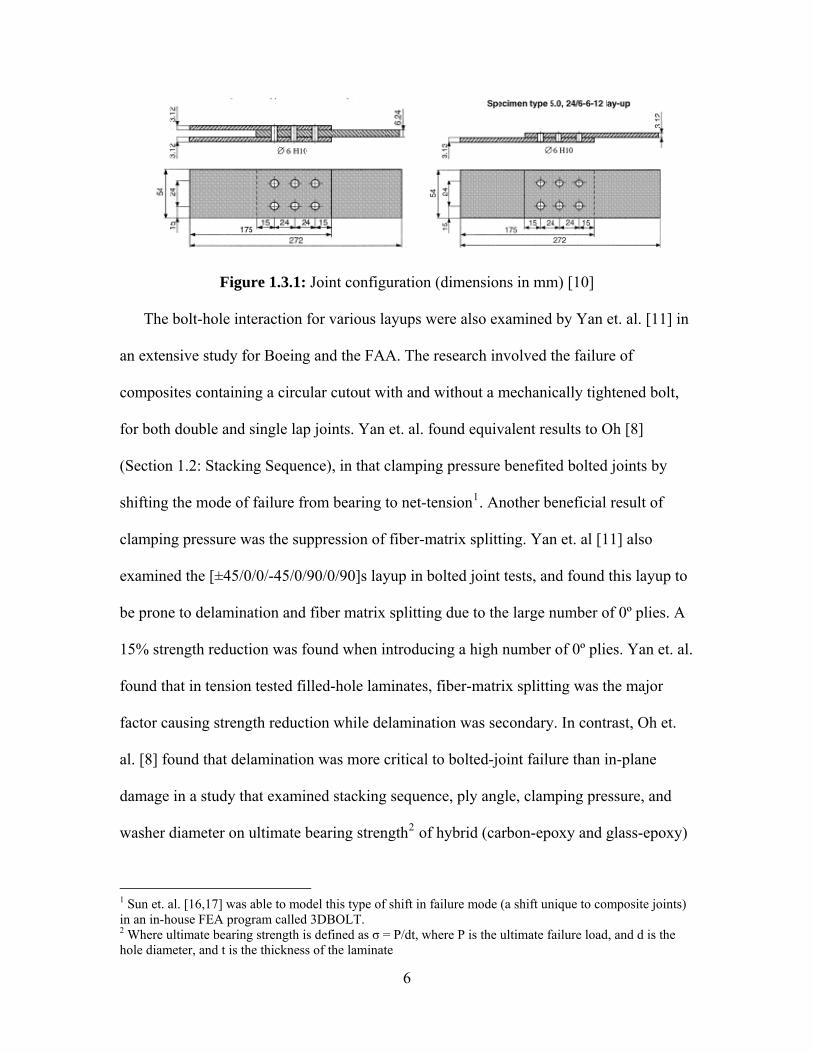
Figure 1.3.1: Joint configuration (dimensions in mm) [10]
The bolt-hole interaction for various layups were also examined by Yan et. al. [11] in
an extensive study for Boeing and the FAA. The research involved the failure of
composites containing a circular cutout with and without a mechanically tightened bolt,
for both double and single lap joints. Yan et. al. found equivalent results to Oh [8]
(Section 1.2: Stacking Sequence), in that clamping pressure benefited bolted joints by
shifting the mode of failure from bearing to net-tension1. Another beneficial result of
clamping pressure was the suppression of fiber-matrix splitting. Yan et. al [11] also
examined the [±45/0/0/-45/0/90/0/90]s layup in bolted joint tests, and found this layup to
be prone to delamination and fiber matrix splitting due to the large number of 0º plies. A
15% strength reduction was found when introducing a high number of 0º plies. Yan et. al.
found that in tension tested filled-hole laminates, fiber-matrix splitting was the major
factor causing strength reduction while delamination was secondary. In contrast, Oh et.
al. [8] found that delamination was more critical to bolted-joint failure than in-plane
damage in a study that examined stacking sequence, ply angle, clamping pressure, and
washer diameter on ultimate bearing strength2 of hybrid (carbon-epoxy and glass-epoxy)
1 Sun et. al. [16,17] was able to model this type of shift in failure mode (a shift unique to composite joints) in an in-house FEA program called 3DBOLT. 2 Where ultimate bearing strength is defined as σ = P/dt, where P is the ultimate failure load, and d is the hole diameter, and t is the thickness of the laminate
6
laminates. This indicates that conclusions drawn for open-hole and filled-hole laminates
are not necessarily applicable to single and double lap bolted joints.
The affects of various layups on through-the-thickness properties were examined by
Kostreva et. al. [12]. An experimental procedure was developed to determine through-
the-thickness compressive (TTTC) material properties for four different graphite/epoxy
material systems. TTTC strength increased as layups were changed from [0], [0/90],
[0/±45/90] and [0/±30/±60/90] (TTTC strengths were unaffected by thickness). Kostreva
found that while the matrix was dominant in determining TTTC modulus, it was also
affected by fiber orientations which doubled the stiffness as layups were changed from
cross ply to quasi-isotropic.
Finite element analysis (FEA) has been used to understand the strain response of
various layups. Dano et. al. [13] developed a finite element model to predict the bearing
response of pin-loaded graphite epoxy composite plates with different isotropic layups.
Non-linear shear behavior was found to be very important for strength prediction of two
layups, [(0/90)6]s and [(±45)6], but only had a slight effect for [(0/±45/90)3]. McCarthy et
al. [14,15] verified a non-linear finite element code MSC.Marc with a 3-D ABAQUS
code and an in-house finite element code entitled STRIPE. The FEA codes modeled a
single bolt, single lap joint with a layup of [45/0/-45/90]5s, and a similar layup with a
higher percentage of 0º plies. All the models predicted the same secondary bending, bolt
tilting, twisting, and through-thickness variations in stress and strain. Surface strain
distribution was not affected by bolt-hole clearance, except at points very close to the
loaded side of the hole. However bolt-hole clearance had a strong effect on the load at
which first significant failure (bearing failure) occurred. Another important finding was
7

that once significant damage has occurred, strain is no longer constant through-the-
thickness. Modeling the gripped area improved the FEA results. A study supporting
McCarthy’s results was performed by Sun et. al. [16, 17] for the effect of washer
clamping area on the ultimate bearing load of a bolt-filled hole. Sun et al. tested a cross
ply layup [(0/90)6] and a quasi-isotropic layup [(0/±45/90)3]. Sun et al. found
experimentally that bolt bearing failure is a 3-D phenomenon, and that joint strength
depends on the initial clamping force in the washer but more importantly on the size of
the clamped area. Sun et. al also found that an increase in the clamping area increased the
ultimate bearing load.
Similar to research on LSS, various layups have been examined in the literature for
bolt-hole interactions, but much less research has quantified the layup’s affect on open-
hole tension strength. What has been presented experimentally often has not been
compared theoretically, or visa-versa. Proprietary constraints make it difficult to compare
the experimental results of one study with the theoretical results of another. Thus, the
current research attempts to compare both experimental and theoretical observations for
the selected non-traditional laminates, and to quantify these results.
1.4: Ply Orientation
The ply orientation may be tailored to increase the strength of composite laminates,
and some literature has examined the open-hole tension loading scenario. Tan [18] tested
the influence of laminate thickness and ply orientation on the strength of graphite epoxy
laminates with circular holes centered in an infinite plate. Tan developed a computer
model using FORTRAN and the Quadratic failure criterion to estimate strength and
optimize the laminate, which successfully represented the behavior of a composite until
8

initial (first ply) failure. Tan found that [0/±29]s had a 41% strength increase over
aluminum. Tsau et. al. [19] used the simplex method to optimize the ply orientations of
four, six, and eight layer laminates, and used the Hashin failure criterion as an objective
function. The simplex method is a direct searching method, appropriate for an
unconstrained optimization problem. The stress components were input into Hashin, and
the objective function values were obtained. A smaller function value meant higher
laminate strength, so the simplex method was used to find a minimum function value.
Tsau found that with properly selected initial angles, the simplex method could be used to
optimize the ply orientations of the four, six, and eight ply laminates. The optimization
was verified by comparing the theoretical and experimental ultimate strengths. However,
above eight plies the error between the predicted optimization and experimental results
became too high for practical purposes. Also, even for some of the four, six, and eight ply
optimizations the error was above ten percent, indicating further study is needed to
control the effectiveness of this method. Barakat et. al. [20] used an energy based failure
criterion developed by Abu-Farsakh and Abdel-Jawad for the strength optimization of the
laminate. Analytical results showed that the laminate configuration was sensitive to the
loading case, that the minimum weight occurred at an orientation where the stresses were
maximum, and that the optimal laminate configuration was always non-symmetric.
The ply orientation of CFRP composites can alter interlaminar and shear strength
properties, as well as material properties such as modulus. Shi, C.H. [21] examined the
interlaminar stresses near the circular hole of open-hole carbon/epoxy symmetric
laminate coupons. Coupons with ply angles of 0º, 15º, 30º, 45º, and 90º were subjected to
in-plane shear. While the maximum interlaminar shear values for the 45º ply angle
9

laminate are generally the lowest, shear results varied largely depending on the location
around the hole and the diameter to thickness ratio. Oh et. al. [8] examined a
[02/θ 3/902]S layup for carbon-epoxy and glass-epoxy laminates where θ was (0/90), ±15º,
±30º, and ±45º ply orientations. Oh et. al. found that [02/(±45)3/902]s was highest in
ultimate bearing strength, and that [02/(±15)3/902]s had the highest modulus. Treasurer
[22] varied the longitudinal (0º) plies in traditional laminates for several loading
scenarios to be non-traditional ±5º or ±10º. In traditional laminates the stress
concentration was redistributed after longitudinal matrix splitting, however in the non-
traditional laminates this splitting was suppressed causing a reduction in strength and
modulus in open-hole tension and compression. However, non-traditional laminates
increased the strength of single-shear bearing due to increased bearing resistance. Muc
[23] analytically investigated the effect of ply orientations for uniaxial and biaxial
compression on the maximum buckling load. Muc used the Love-Kirchhoff hypothesis to
obtain the optimized laminate, which depended on the buckling mode, geometry, and
material properties.
Much less literature is available for the influence of ply orientation on open-hole
tension strength than for the influence of LSS or layup on strength. The literature that has
examined ply orientation is typically confined to a few angles [21, 22], and optimization
programs are also limited by number of plies [19]. The focus of the current study is to
select optimized non-traditional laminates from all possible ply orientation angles (0º to
90º), and to produce a large volume of experimental strength and strain field results.
10

1.5: Failure Criteria
Failure criteria have been used in literature to predict the strength of CFRP
composites. Dano et. al. [13] observed that when the shear stress is large, the Hashin
criterion is more conservative than the maximum stress criterion. However, when the
shear stress strain curve is linear, maximum stress criterion predicts higher and more
accurate strength than Hashin Criterion. Dano et. al proposed a mixed failure criteria and
associated table of degradation rules for pin-loaded composites.
Park [6,7] uses Ye-delamination failure criterion based on layerwise finite element
contact stress analysis to predict the bearing failure strengths of mechanically fastened
joints. The predicted strengths are lower than experimental strengths, a difference which
increases as clamping pressure increases. The predicted and measured values stay within
6-10%.
A recently proposed strain invariant failure theory (SIFT) shows promise for
modeling progressive damage and predicting strength in carbon fiber-epoxy specimens,
and may avoid many problems associated with other failure criteria. Previous methods
have used failure criteria to degrade properties in the stiffness matrix of failed FEA
elements. These material property degradation methods (MPDMs) are generally high in
computational demand3, and their solutions do not always converge. Gosse [24] used
SIFT with a damage function methodology to obtain the maximum energy retention
(MER, which corresponds to maximum load capacity of the strained specimen). This
theory is based on the idea that solids fail by excessive deformation. The MER
methodology was successfully demonstrated with normalized data from open-hole
3 When using an MPDM, commercial codes such as ABAQUS must recalculate entire meshes iteratively when properties are degraded causing a high computation demand.
11

compression, open-hole tension, filled-hole tension, large-notch tension, and large-notch
compression tests.
Tay et. al. [5] used the SIFT based Element-Failure Method (EFM) to avoid problems
associated with the MPDM and to present a simpler finite element approach. The
Element Failure Method (EFM) modifies nodal forces in a finite element model to reflect
the general state of damage and loading. Tay et. al. found that nodal force modification in
the thickness direction is needed to correctly predict interlaminar damage, supporting the
notion that composite damage progression is a complex three dimensional process. Tay’s
finite element model was in-house due to user constraints in the commercial code
ABAQUS (Tay et. al., [25]). Implementation of the SIFT-MER-EFM approach has been
demonstrated for many test scenarios and allows for both mechanical and environmental
loading (thermal residual strains).
1.5.1: Mode-based Failure Criteria
The Maximum Stress and Maximum Strain Criteria are dependent on the failure
strength of the lamina [26]. The Maximum Stress Criterion is based on the inequalities
(1.5.1) )(
111)(
1+− << ss σ
(1.5.2) )(222
)(2
+− << ss σ
1212 s<τ , (1.5.3)
where s1, s2, and s12 are the ultimate longitudinal, transverse, and shear strengths,
respectively, in tension (+) and compression (-), and σ11, σ22, and τ12 are the in-plane
stresses.
Similarly, the Maximum Strain Criterion is based on the strength of the lamina in
terms of engineering strain:
12

(1.5.4) )(111
)(1
+− << ee ε
(1.5.5) )(222
)(2
+− << ee ε
1212 e<γ , (1.5.6)
where e1, e2, and e12 are the ultimate longitudinal, transverse, and shear strains,
respectively, in tension (+) and compression (-), and ε11, ε22, and γ12 are the in-plane
strains. In these ply-by-ply failure criteria, analysis is confined to in-plane fracture.
Possible interaction between stress components, crack propagation between plies, and
delamination is neglected in the two dimensional form of the criteria.
Hashin [27] proposed a piecewise criterion to account for possible failure modes of
the composite. For plane stress, the fiber-mode failure in tension (σ11>0) is
12
12
12
2
)(1
11 =⎟⎟⎠
⎞⎜⎜⎝
⎛+⎟⎟
⎠
⎞⎜⎜⎝
⎛+ ss
τσ . (1.5.7)
For fiber-mode failure under compression (σ11<0) this becomes
12
)(1
11 =⎟⎟⎠
⎞⎜⎜⎝
⎛−s
σ . (1.5.8)
Similar equations are defined for the matrix-mode failure, and for plane stress under
tension (σ22>0) this is
12
12
12
2
)(1
22 =⎟⎟⎠
⎞⎜⎜⎝
⎛+⎟⎟
⎠
⎞⎜⎜⎝
⎛+ ss
τσ . (1.5.9)
For matrix-mode failure under compression (σ22<0) this becomes
1122
2
12
12)(
2
22
2
23
)(2
2
23
22 =⎟⎟⎠
⎞⎜⎜⎝
⎛+⎟⎟⎠
⎞⎜⎜⎝
⎛
⎥⎥⎦
⎤
⎢⎢⎣
⎡−⎟⎟
⎠
⎞⎜⎜⎝
⎛+⎟⎟
⎠
⎞⎜⎜⎝
⎛−
−
ssss
sσσσ . (1.5.10)
13

1.5.2: Quadratic Interaction Failure Criteria
Quadratic criteria differ from limit criteria because they use quadratic terms to
account for the interaction of stress components. While these terms are meant to mimic
the stress interaction in the composite, it is important to remember that these criteria are
purely empirical. Hill [28] was one of the first to suggest such a criterion. He modified
the von Mises Criterion for isotropic metals to include anisotropy in the equation
, (1.5.11) 1222)()()( 212
231
223
22211
21133
23322 =+++−+−+− τττσσσσσσ FEDCBA
where A, B, C, D, E, and F are constants based on yield strength, and defined in [28]. The
Hill Criterion was modified by Tsai [30] to assume plane stress in a transversely isotropic
lamina as
1212
212
22
222
21
221121
211 =++−
ssssτσσσσ , (1.5.12)
and is referred to as the Tsai-Hill Criterion [26]. Generalization of the von Mises criterion
for orthotropic material lacks analytic basis [30], resulting in 6 independent strength
components instead of 9. Hoffman [31] added linear stress terms to the Tsai-Hill
Criterion in order to account for unequal stresses in tension and compression [26, 32],
and the result was
22)(2
)(2
11)(1
)(1
2
12
12)(
2)(
2
222
)(11
)(11
2211)(
1)(
1
211 1111
2σστσ
σσσσσ
⎟⎟⎠
⎞⎜⎜⎝
⎛−+⎟⎟
⎠
⎞⎜⎜⎝
⎛−+⎟⎟
⎠
⎞⎜⎜⎝
⎛++− −+−+−+−+−+ sssssssss
. (1.5.13)
Tsai and Wu [30] proposed a tensor polynomial theory for anisotropic materials of
the form of
1=+ jiijii FF σσσ . (1.5.14)
14

This equation accounts for tensile and compressive stress induced failures, allowing the
failure curve to be represented in a single function. Under plane stress the Tsai-Wu
Criterion becomes
, (1.5.15) 12 2211122221121266
22222
21111 =+++++ σσσστσσ FFFFFF
where the Fij and Fi terms are found from uniaxial and shear strength tests and are
)(1
)(1
111
−+=ss
F ,
)(1
)(1
111−+ −=
ssF ,
)(
2)(
222
1−+=
ssF ,
)(2
)(2
211−+ −=
ssF ,
212
661s
F = . (1.5.16)
F12 was modified by Tsai and Hahn [33] to be
2)( 2/1
221112
FFF −= (1.5.17)
to avoid a complicated biaxial test and optimization procedure required by the original criterion. Yamada-Sun simplified the Tsai criterion for unidirectional materials [32] to
12
12
12
2
)(1
11 =⎟⎟⎠
⎞⎜⎜⎝
⎛+⎟⎟
⎠
⎞⎜⎜⎝
⎛+ ss
τσ . (1.5.18)
Quadratic criteria are fundamentally curve fits, with quadratic terms manipulated to
represent stress interactions. It is important to note that these terms aren’t based on
specific failure modes, but rather experimental data.
1.5.3: Failure Criteria versus Experimental Results
Failure criteria have shown useful results for some loading scenarios, and inadequate
results for others. Kam and Sher [34] studied the first ply failure and nonlinear behavior
of cross-ply laminated composite plates, and examined the energy based von Karman
Plate theory, the Maximum Stress, Maximum Strain, Hoffman, Tsai-Hill, and Tsai-Wu
15

Criteria. Matrix cracking was found to be a major factor leading to stiffness reduction,
and inconsistent results indicated that the strength-of-material approach to first-ply failure
prediction was insufficient. Treasurer [22] found that the Tsai-Wu Criterion predicted
experimental results for non-traditional laminates better than the Hashin or Maximum
Stress Criteria.
Soden et. al. [1] organized a World Wide Failure Exercise (WWFE) to test the
validity of 19 leading composite strength theories. Of these, the top 5 theories were
evaluated and recommendations on their applicability were made. The top 5 included the
theories of Zinoviev [35], Bogetti [36], Puck [37], Cuntze [38], and Tsai [39]. Theoretical
and experimental agreement for initial failure was considered poor, partly due to lack of
reliable experimental data, disagreement between definitions of initial failure, and not
enough attention given to residual thermal stresses4. Bogetti and Zinoviev ranked best for
initial failure in multidirectional laminates. Puck partially allowed for thermal stresses,
and his theory yielded conservative predictions. For final failure, none of the theories in
the WWFE could predict within ±10% of strength for more than 40% of the test cases. In
general, the theories were less accurate when shear stress and matrix behavior were
significant, and where large deformation occurred before failure. However, some theories
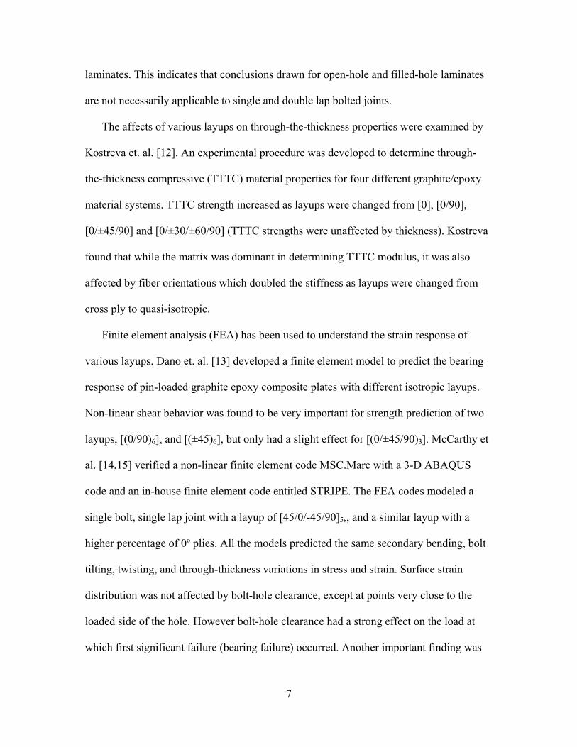
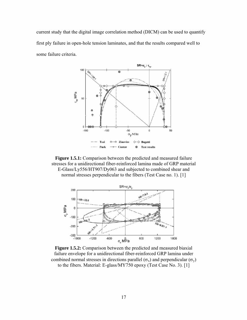
did well for predicting some test cases, as shown in Figures 1.5.1-1.5.3. The WWFE
findings were published in 2004, and this was one of the largest failure criteria studies to
date. The WWFE was useful in determining the weaknesses of current failure theories,
and the direction that composite research should pursue. One of the weaknesses
addressed was the lack of theoretical and experimental definitions for initial (first ply)
failure, and corresponding lack of reliable experimental data. It will be found in the 4 Residual thermal stresses can be introduced in curing, and when moisture exists.
16
current study that the digital image correlation method (DICM) can be used to quantify
first ply failure in open-hole tension laminates, and that the results compared well to
some failure criteria.
Figure 1.5.1: Comparison between the predicted and measured failure stresses for a unidirectional fiber-reinforced lamina made of GRP material
E-Glass/Ly556/HT907/Dy063 and subjected to combined shear and normal stresses perpendicular to the fibers (Test Case no. 1). [1]
Figure 1.5.2: Comparison between the predicted and measured biaxial failure envelope for a unidirectional fiber-reinforced GRP lamina under
combined normal stresses in directions parallel (σx) and perpendicular (σy) to the fibers. Material: E-glass/MY750 epoxy (Test Case No. 3). [1]
17
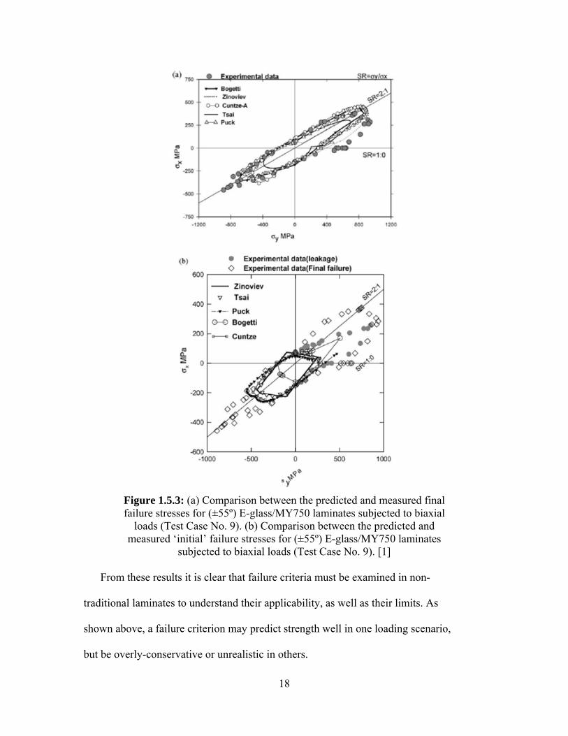
Figure 1.5.3: (a) Comparison between the predicted and measured final failure stresses for (±55º) E-glass/MY750 laminates subjected to biaxial
loads (Test Case No. 9). (b) Comparison between the predicted and measured ‘initial’ failure stresses for (±55º) E-glass/MY750 laminates
subjected to biaxial loads (Test Case No. 9). [1]
From these results it is clear that failure criteria must be examined in non-
traditional laminates to understand their applicability, as well as their limits. As
shown above, a failure criterion may predict strength well in one loading scenario,
but be overly-conservative or unrealistic in others.
18

1.6: Failure Progression
Failure in multidirectional laminates is a progressive and three-dimensional process.
First ply failure often occurs in the form of intralaminar matrix cracks such as matrix
splitting. Intralaminar cracks do not always degrade strength, but may promote other
forms of damage. Under fatigue loading, these cracks may propagate into adjacent plies.
When the cracks span the thickness of several off-axis plies, they can cause a stress
concentration in the load bearing 0º plies, resulting in a reduction of tensile strength [2].
Intralaminer cracks may also couple with interlaminar matrix failure (delamination), to
completely isolate a ply or group of plies. Delamination is prone to initiate at the free-
edges of the coupon. Various forms of tensile damage are shown in Fig. 1.6.1. Even when
matrix cracking does not degrade strength, it may alter properties such as thermal
expansion, liquid permeability, and oxidative stability.
Figure 1.6.1: Failure mechanisms for laminates loaded in tension [2]
19

Damage becomes more complicated with the introduction of a hole due to a bolt or
rivet. Matrix damage and fiber matrix splitting at the hole may actually increase the
ultimate tensile strength because the stress is redistributed. This often occurs in “hard
laminates,” which have an increased number of 0º plies. During the stress redistribution,
material stiffness is reduced [2]. Treasurer [22] also found this softening effect during the
stress redistribution of hard laminates. The decrease in material stiffness was verified in
the current study, as will be shown in Chapter 5. Treasurer [22] also found that replacing
longitudinal plies with off-axis plies (±5º and ±10º) in open-hole tension suppressed this
stress redistribution and decreased strength. However, Treasurer found a 23% and 25%
strength increase for the ±5º and ±10º longitudinal ply replacements in single-shear
bearing. The slightly off-axis plies added bearing resistance compared to the traditional
layups.
1.7: Conclusion
As shown in the literature review, much research has been done considering fastener
design. Studies may also be found focusing on the effect of stress concentrations in
composites. However, much of this work has concentrated on the interaction of the bolt
and the hole. Research that concerns itself with ply orientation generally only considers
changing the number of plies in standard layups, or comparing standard layups with one
another. Less work attempted to tailor the ply orientation to increase strength, which is
the focus of the current study.
The results in literature for open-hole tension are often limited by proprietary
constraint, lack of theoretical and experimental comparison, or limits in reliability (as in
the case of initial failure). The current study examines numerous non-traditional
20

laminates in open-hole tension and the corresponding interaction between the LSS, layup,
and ply orientation near the hole. Experimental results are compared to theoretical
predictions, as well as to results available in literature. It will be shown that the laminate
may be tailored to increase strength using tools readily available in industry, and that the
digital image correlation method is a valuable tool for locating first ply failure in
experimental research.
21
2: Finite Element Analysis
2.1: Finite Element Model
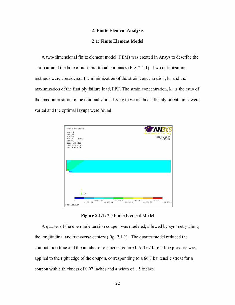
A two-dimensional finite element model (FEM) was created in Ansys to describe the
strain around the hole of non-traditional laminates (Fig. 2.1.1). Two optimization
methods were considered: the minimization of the strain concentration, kt, and the
maximization of the first ply failure load, FPF. The strain concentration, kt, is the ratio of
the maximum strain to the nominal strain. Using these methods, the ply orientations were
varied and the optimal layups were found.
Figure 2.1.1: 2D Finite Element Model
A quarter of the open-hole tension coupon was modeled, allowed by symmetry along
the longitudinal and transverse centers (Fig. 2.1.2). The quarter model reduced the
computation time and the number of elements required. A 4.67 kip/in line pressure was
applied to the right edge of the coupon, corresponding to a 66.7 ksi tensile stress for a
coupon with a thickness of 0.07 inches and a width of 1.5 inches.
22
Figure 2.1.2: Boundary Conditions
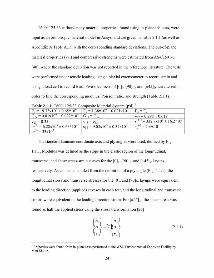
The finite element model was constructed using a linear Shell99 element (Fig. 2.1.3).
This element allows the input of either the ply orientations or the ABD matrix (from
classical lamination theory) to describe the layup. Shell99 is designed for layered
applications of two-dimensional structural shell models, appropriate for thin laminates.
The element has eight nodes (four corner, four midside), one element through the
thickness, and six degrees of freedom per node. Shell99 has less element formulation
time than other shell elements (Shell91) because it doesn’t have nonlinear capabilities.
Figure 2.1.3: Shell99 Element (© Ansys 2006)
23
T600: 125-33 carbon/epoxy material properties, found using in-plane lab tests, were
input as an orthotropic material model in Ansys, and are given in Table 2.1.1 (as well as
Appendix A Table A.1), with the corresponding standard deviations. The out-of-plane
material properties (ν23) and compressive strengths were estimated from AS4/3501-6
[40], where the standard deviation was not reported in the referenced literature. The tests
were performed under tensile loading using a biaxial extensometer to record strain and
using a load cell to record load. Five specimens of [0]6, [90]16, and [±45]2s were tested in
order to find the corresponding modulus, Poisson ratio, and strength (Table 2.1.1).
Table 2.1.1: T600: 125-33 Composite Material System (psi) 5 E1 = 19.73x10⁶ ± 0.65*106 E2 = 1.38x10⁶ ± 0.021x10⁶ E3 = E2 G12 = 0.81x10⁶ ± 0.022*106 G13 = G12 ν12 = 0.298 ± 0.019 ν23 = 0.35 ν13 = ν12 sL
(+) = 332.8x10³ ± 16.2*103
sT(+) = 6.28x10³ ± 0.63*103 sLT = 9.03x10³ ± 0.37x10³ sL
(-) = 209x103
sT(-) = 33x103
The standard laminate coordinate axis and ply angles were used, defined by Fig.
1.1.1. Modulus was defined as the slope in the elastic region of the longitudinal,
transverse, and shear stress-strain curves for the [0]6, [90]16, and [±45]2s layups,
respectively. As can be concluded from the definition of a ply angle (Fig. 1.1.1), the
longitudinal stress and transverse stresses for the [0]6 and [90]16 layups were equivalent
to the loading direction (applied) stresses in each test, and the longitudinal and transverse
strains were equivalent to the loading direction strain. For [±45]2s, the shear stress was
found as half the applied stress using the stress transformation [26]
(2.1.1) [ ]⎪⎭
⎪⎬
⎫
⎪⎩
⎪⎨
⎧
=⎪⎭
⎪⎬
⎫
⎪⎩
⎪⎨
⎧
xy
y
x
T
τ
σσ
τσσ
12
2
1
5 Properties were found from in-plane tests performed at the WSU Environmental Exposure Facility by Matt Shultz.
24

where the transformation matrix [T] is given by
(2.1.2) [ ]⎥⎥⎥
⎦
⎤
⎢⎢⎢
⎣
⎡
−−−=
22
22
22
22
sccscscscs
csscT
with c=cos(θ) s=sin(θ). Subsituting σx=τxy=0 for the [(±45)2]s loading scenario
( ) ( )2
º45sinº45cos12x
xσστ −=−= . (2.1.3)
Similarly, the shear strain is found using the strain transformation [26]
, (2.1.4) [ ]⎪⎭
⎪⎬
⎫
⎪⎩
⎪⎨
⎧
=⎪⎭
⎪⎬
⎫
⎪⎩
⎪⎨
⎧
2/2/12
2
1
xy
y
x
T
γ
εε
γεε
and solving for the shear strain we obtain
( ) ( ) ( ) ( )( )2
º45sinº45cosº45sinº45cos)º45sin()º45cos(2
2212 xyyx
γεεγ
−++−= . (2.1.5)
This reduces to
yx εεγ +−=12 , (2.1.6)
which shows that the shear strain for the [±45]2s test can be found from the sum of the
longitudinal and transverse strains, measured by the biaxial extensometer. The
longitudinal and transverse strengths were defined as the ultimate tensile strength
(Appendix A Table A.1). The shear strength was defined as the stress corresponding to
50,000 με, according to ASTM D3518 (discussed further in Section 5.3).
The dimensions for the baseline coupon are those of a standard open-hole tension
coupon (Appendix B), with a baseline layup of [(45/90/-45/0)2]s. This baseline layup is
shown ply-by-ply for half the laminate in Fig. 2.1.4 (the other half of the laminate is
25

symmetric to this). The 2D FEA in Ansys models these plies at the same location, so that
through-the-thickness effects are not accounted for. The plies can be easily altered for a
given layup, and the computation is under a minute. Thus, the 2D FEA is ideal for
analysis of a large number of layups, as in optimization considering all ply angles from 0º
to 90º.
Figure 2.1.4: Ply orientations in Ansys
The final mesh geometry was found to be optimal during the development of the
FEM, and contains 4,600 elements (Fig. 2.1.5). Other mesh shapes and configurations
distorted the strain contours near the hole, thus the triangular mesh areas at the hole were
extended to 0.75 inches from the hole center. At this mesh boundary, the stress
concentration of the hole had dissipated enough so that the strain contours are not
adversely affected by the mesh boundary. The convergence study (Appendix C) showed
that further mesh refinement is not necessary, as the solution was not altered by adding
more elements. The mesh was more refined at the hole due to the high strain gradients at
the stress concentration, and gradually became less refined away from the hole.
26

Figure 2.1.5: Final Mesh
2.2: Optimization Methods
Two optimization methods were used: the reduction of the strain concentration factor,
kt, in order to increase the strength of the laminate, and the use of the Maximum Strain
Criterion to increase the first ply failure load, FPF. The optimization curves for these
methods are shown in Appendix D and are described in Section 2.4. To define the stress
concentration, the maximum strain was taken at the top of the hole (0, 0.125), and the
nominal strain as taken at a point away from all edges where the strain reaches a constant
level (Fig. 2.2.1).
27
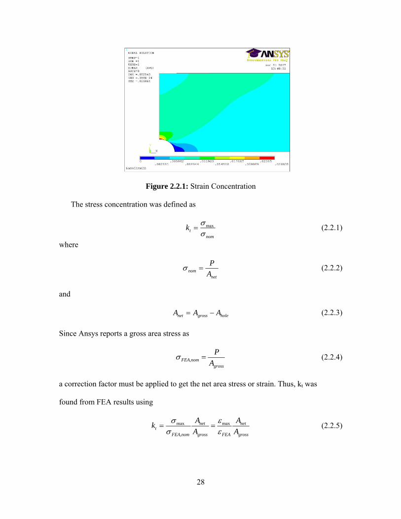
Figure 2.2.1: Strain Concentration
The stress concentration was defined as
nom
tkσσmax= (2.2.1)
where
net
nom AP
=σ (2.2.2)
and
holegrossnet AAA −= (2.2.3) Since Ansys reports a gross area stress as
gross
nomFEA AP
=,σ (2.2.4)
a correction factor must be applied to get the net area stress or strain. Thus, kt was
found from FEA results using
gross
net
FEAgross
net
nomFEAt A
AAAk
εε
σσ max
,
max == (2.2.5)
28
An alternative method for calculating kt, sometimes used in industry, is to apply a width
correction factor to a plate of infinite width. This is a more generally applicable method
because a width correction factor can be applied to the infinite plate results for any
number of geometries. If the appropriate correction factor is applied for the current
geometry, the infinite plate kt is approximately equivalent to the kt calculated from eq.
2.2.5. The dimensions of the open-hole tension coupon did not change for the current
study, so eq. 2.2.5 was used because it incorporates the coupon geometry and edge
effects.
In two dimensional FEA, the stress depends on the ply orientation and changes for
each ply, whereas the strain remains constant in the absence of through-the-thickness
effects. Therefore, a stress-based kt would require an average of the kt for each ply,
whereas a strain-based kt would be equivalent to the kt of any ply. Thus, the strain-based
kt was preferred for the current study so that only the strain data from the surface ply was
needed.
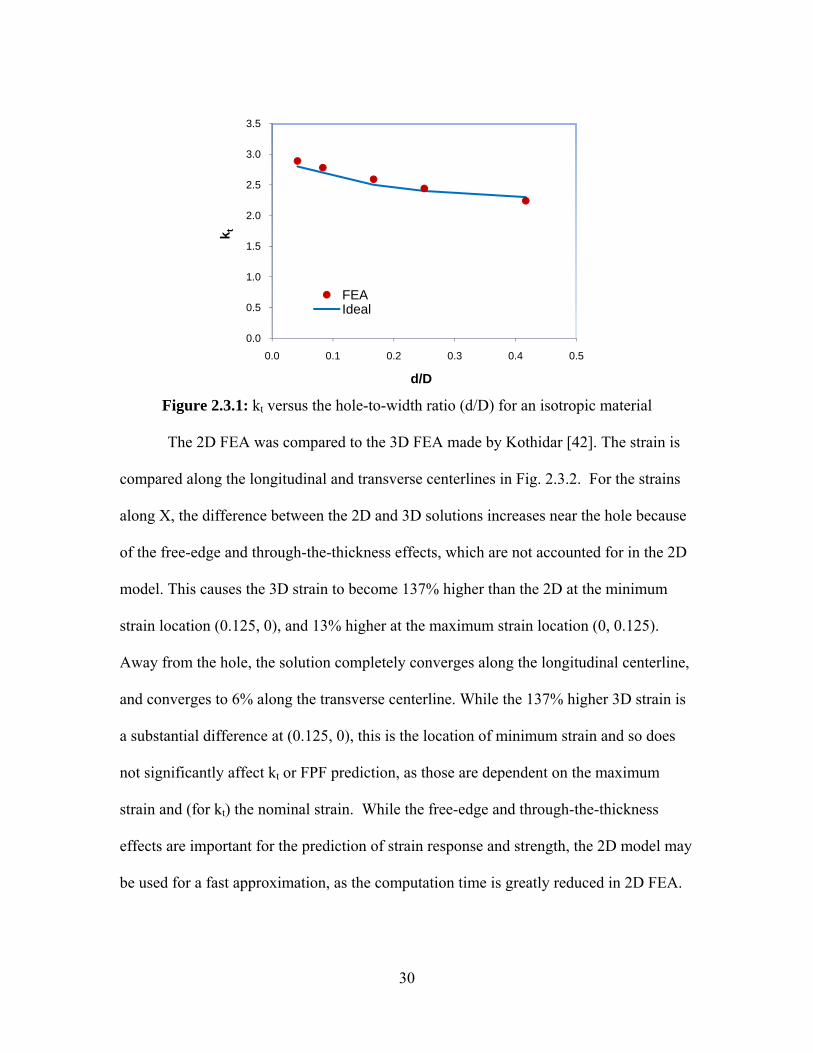
2.3: Model Verification
Aluminum material properties (Appendix A) were input into the FEM, and the kt
was found to be 2.59 for the given coupon geometry (Appendix B). This is near the
analytical value of 2.50 for an isotropic material with the same hole/width (d/D) ratio
[41]. The width was then varied and compared to analytical values, as shown in Fig.
2.3.1.
29
0.0
0.5
1.0
1.5
2.0
2.5
3.0
3.5
0.0 0.1 0.2 0.3 0.4 0.5
k t
d/D
FEAIdeal
Figure 2.3.1: kt versus the hole-to-width ratio (d/D) for an isotropic material
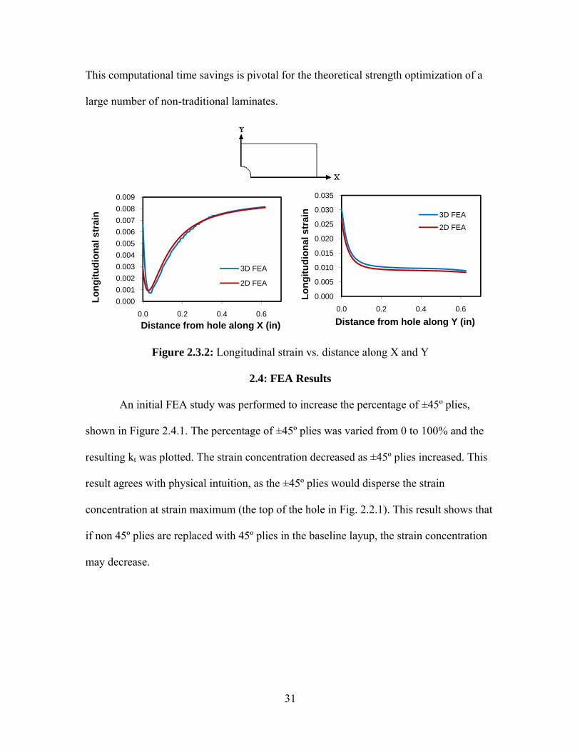
The 2D FEA was compared to the 3D FEA made by Kothidar [42]. The strain is
compared along the longitudinal and transverse centerlines in Fig. 2.3.2. For the strains
along X, the difference between the 2D and 3D solutions increases near the hole because
of the free-edge and through-the-thickness effects, which are not accounted for in the 2D
model. This causes the 3D strain to become 137% higher than the 2D at the minimum
strain location (0.125, 0), and 13% higher at the maximum strain location (0, 0.125).
Away from the hole, the solution completely converges along the longitudinal centerline,
and converges to 6% along the transverse centerline. While the 137% higher 3D strain is
a substantial difference at (0.125, 0), this is the location of minimum strain and so does
not significantly affect kt or FPF prediction, as those are dependent on the maximum
strain and (for kt) the nominal strain. While the free-edge and through-the-thickness
effects are important for the prediction of strain response and strength, the 2D model may
be used for a fast approximation, as the computation time is greatly reduced in 2D FEA.
30
This computational time savings is pivotal for the theoretical strength optimization of a
large number of non-traditional laminates.
0.0000.0010.0020.0030.0040.0050.0060.0070.0080.009
0.0 0.2 0.4 0.6
Long
itudi
onal
str
ain
Distance from hole along X (in)
3D FEA
2D FEA
0.000
0.005
0.010
0.015
0.020
0.025
0.030
0.035
0.0 0.2 0.4 0.6Lo
ngitu
dion
al s
trai
n
Distance from hole along Y (in)
3D FEA2D FEA
Figure 2.3.2: Longitudinal strain vs. distance along X and Y
2.4: FEA Results
An initial FEA study was performed to increase the percentage of ±45º plies,
shown in Figure 2.4.1. The percentage of ±45º plies was varied from 0 to 100% and the
resulting kt was plotted. The strain concentration decreased as ±45º plies increased. This
result agrees with physical intuition, as the ±45º plies would disperse the strain
concentration at strain maximum (the top of the hole in Fig. 2.2.1). This result shows that
if non 45º plies are replaced with 45º plies in the baseline layup, the strain concentration
may decrease.
31

Figure 2.4.1: kt vs. the percentage of 45º plies for the baseline layup
2.002.503.003.504.004.505.005.506.00
0% 20% 40% 60% 80% 100%
kt%45º
The Maximum Strain Criterion, discussed in Section 1.6, was used to predict FPF.
This is because the Maximum Strain Criterion best predicted the initial fabricated set of
kt-optimized non-traditional laminates, and was thus used for the second fabricated set of
FPF-optimized non-traditional laminates. The strain data from Ansys for a given layup
was input into a failure criteria Matlab program (Appendix E), which included the
Maximum Strain Criterion and several other common failure criteria, detailed in Section
1.6 and 1.7. The Matlab program was created with the use of Ref. [32]. The program
inputs were the strain state at a locations of interest, the ply orientations of the laminate,
and the load. The strain and corresponding stresses were transformed into the fiber
direction coordinate system for each ply using the transformation matrix of equations
2.1.1, 2.1.2, and 2.1.4 from Ref. [26]. The stress or strain was then applied to each
strength criterion for each ply. Since balanced orientations (±45º) produced the same
failure index, the absolute value of the ply orientations was used so that only one set of
tensile and compressive strengths were needed for a given failure criterion and strain
state. The in-plane allowable stresses were found in laboratory tests (Appendix A),
described in Section 2.1. These strengths were divided by the appropriate modulus to get
allowable strains for the strain based criteria. Nonlinear effects were ignored in the
current study to simplify analysis and decrease computation time, but would have some
32
influence on the strain state and thus the failure criteria. Using a given failure criterion,
the failure index was calculated and used to find strength by
..if
s appliedσ= (2.4.1)
where σapplied is the applied stress, s is the strength, and f.i. is the failure index. The
outputs of the Matlab program were the kth ply failure load and the corresponding failure
mode6 (for mode-based criteria).
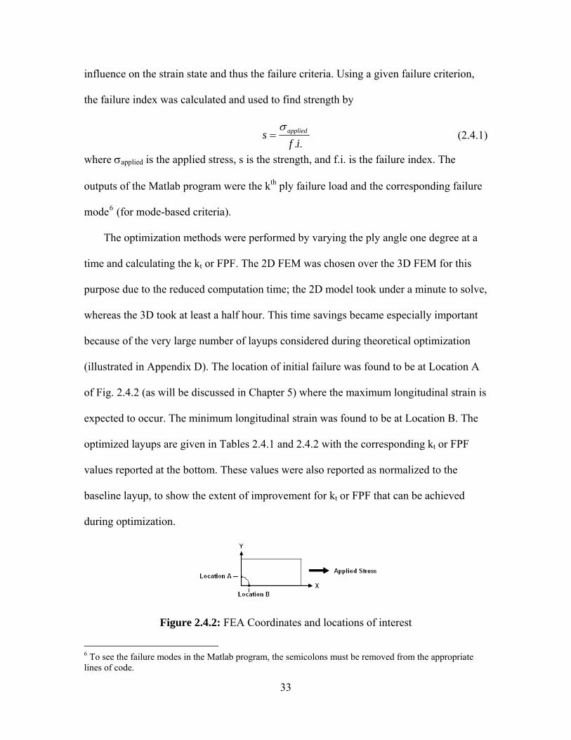
The optimization methods were performed by varying the ply angle one degree at a
time and calculating the kt or FPF. The 2D FEM was chosen over the 3D FEM for this
purpose due to the reduced computation time; the 2D model took under a minute to solve,
whereas the 3D took at least a half hour. This time savings became especially important
because of the very large number of layups considered during theoretical optimization
(illustrated in Appendix D). The location of initial failure was found to be at Location A
of Fig. 2.4.2 (as will be discussed in Chapter 5) where the maximum longitudinal strain is
expected to occur. The minimum longitudinal strain was found to be at Location B. The
optimized layups are given in Tables 2.4.1 and 2.4.2 with the corresponding kt or FPF
values reported at the bottom. These values were also reported as normalized to the
baseline layup, to show the extent of improvement for kt or FPF that can be achieved
during optimization.
Figure 2.4.2: FEA Coordinates and locations of interest
6 To see the failure modes in the Matlab program, the semicolons must be removed from the appropriate lines of code.
33
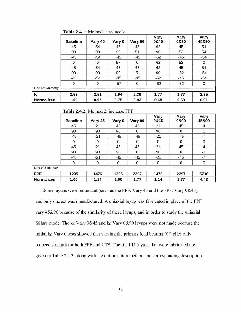
Table 2.4.1: Method 1: reduce kt
Baseline Vary 45 Vary 0 Vary 90 Vary 0&45
Vary 0&90
Vary 45&90
45 54 45 45 62 45 54 90 90 90 51 90 52 54 -45 -54 -45 -45 -62 -45 -54 0 0 57 0 62 52 0 45 54 45 45 62 45 54 90 90 90 -51 90 -52 -54 -45 -54 -45 -45 -62 -45 -54 0 0 -57 0 -62 -52 0 Line of Symmetry ------------------------------------------------------------------------------------------------------------------------------------------------
kt 2.58 2.51 1.94 2.39 1.77 1.77 2.35 Normalized 1.00 0.97 0.75 0.93 0.68 0.69 0.91 Table 2.4.2: Method 2: increase FPF
Baseline Vary 45 Vary 0 Vary 90 Vary 0&45
Vary 0&90
Vary 45&90
45 21 45 45 21 45 4 90 90 90 0 90 0 1 -45 -21 -45 -45 -21 -45 -4 0 0 0 0 0 0 0 45 21 45 45 21 45 4 90 90 90 0 90 0 -1 -45 -21 -45 -45 -21 -45 -4 0 0 0 0 0 0 0 Line of Symmetry -----------------------------------------------------------------------------------------------------------------------------------------------
FPF 1295 1476 1295 2297 1476 2297 5736 Normalized 1.00 1.14 1.00 1.77 1.14 1.77 4.43
Some layups were redundant (such as the FPF: Vary 45 and the FPF: Vary 0&45),
and only one set was manufactured. A uniaxial layup was fabricated in place of the FPF
vary 45&90 because of the similarity of these layups, and in order to study the uniaxial
failure mode. The kt: Vary 0&45 and kt: Vary 0&90 layups were not made because the
initial kt: Vary 0 tests showed that varying the primary load bearing (0º) plies only
reduced strength for both FPF and UTS. The final 11 layups that were fabricated are
given in Table 2.4.3, along with the optimization method and corresponding description.
34

Table 2.4.3: Fabricated layups7 Designation Layup Method Description
BL [(45/90/-45/0)2]s Quasi-isotropic Baseline A [(54/90/-54/0)2]s kt Vary 45º B [(45/51/-45/0)2]s kt Vary 90º C [(45/0/-45/90)2]s Stacking sequence Vary Order 1 D [(45/90/-45/57)2]s kt Vary 0º E [(54/54/-54/0)2]s FPF Vary 45º & 90º F [(45/-45/90/0)2]s Stacking sequence Vary Order 2 G [(21/90/-21/0)2]s FPF Vary 45º H [(45/0/-45/0)2]s FPF Vary 90º I [(±45)4]s Failure mode Shear failure J [0]16 Failure mode Uniaxial failure
The optimization schemes did not impose limits on the variation in material
properties of the resulting non-tradiational laminates compared to baseline. The predicted
values of the material properties (using CLT) are given in Appendix A, and are shown in
Fig. 2.4.3 normalized to baseline. The material properties of the I and J layups vary the
largest, as expected for failure-mode layups that are designed to focus on a specific
material property. While some layups do not vary much from baseline, others show large
variation, such as the H layup. These variations will be discussed and compared to
strength results in Chapter 5. Imposing limits during the optimization process (such as a
limit of 10% variation in modulus that might be imposed in industry), could easily be
done using CLT. However, for the current study, these limits were not imposed in order
to understand the full effect of the optimization methods.
7 The layups are all balanced (the same number of +/- plies on either side of the center line).
35

0.00
0.50
1.00
1.50
2.00
2.50
3.00
3.50
BL A B C D E F G H I J
Normalized
Value
Ex
Ey
vxy
Gxy
Figure 2.4.3: Material properties from CLT of non-traditional laminates normalized to the baseline (BL) layup
36
3: Digital Image Correlation Method
3.1: Experimental Technique
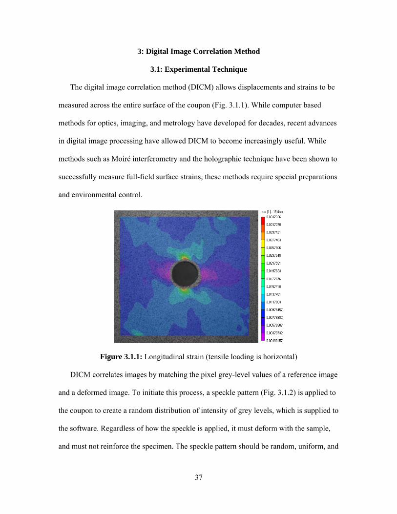
The digital image correlation method (DICM) allows displacements and strains to be
measured across the entire surface of the coupon (Fig. 3.1.1). While computer based
methods for optics, imaging, and metrology have developed for decades, recent advances
in digital image processing have allowed DICM to become increasingly useful. While
methods such as Moiré interferometry and the holographic technique have been shown to
successfully measure full-field surface strains, these methods require special preparations
and environmental control.
Figure 3.1.1: Longitudinal strain (tensile loading is horizontal)
DICM correlates images by matching the pixel grey-level values of a reference image
and a deformed image. To initiate this process, a speckle pattern (Fig. 3.1.2) is applied to
the coupon to create a random distribution of intensity of grey levels, which is supplied to
the software. Regardless of how the speckle is applied, it must deform with the sample,
and must not reinforce the specimen. The speckle pattern should be random, uniform, and
37
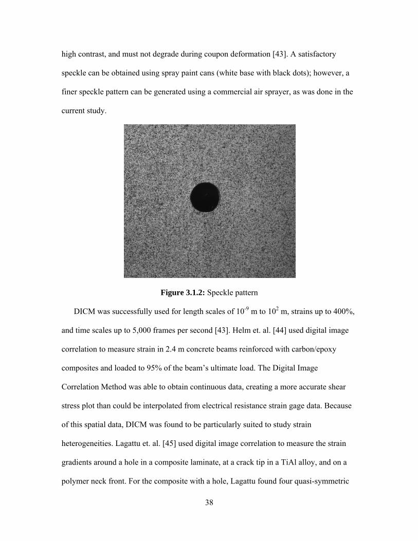
high contrast, and must not degrade during coupon deformation [43]. A satisfactory
speckle can be obtained using spray paint cans (white base with black dots); however, a
finer speckle pattern can be generated using a commercial air sprayer, as was done in the
current study.
Figure 3.1.2: Speckle pattern
DICM was successfully used for length scales of 10-9 m to 102 m, strains up to 400%,
and time scales up to 5,000 frames per second [43]. Helm et. al. [44] used digital image
correlation to measure strain in 2.4 m concrete beams reinforced with carbon/epoxy
composites and loaded to 95% of the beam’s ultimate load. The Digital Image
Correlation Method was able to obtain continuous data, creating a more accurate shear
stress plot than could be interpolated from electrical resistance strain gage data. Because
of this spatial data, DICM was found to be particularly suited to study strain
heterogeneities. Lagattu et. al. [45] used digital image correlation to measure the strain
gradients around a hole in a composite laminate, at a crack tip in a TiAl alloy, and on a
polymer neck front. For the composite with a hole, Lagattu found four quasi-symmetric
38

zones of high strains along the ±45 axes. Lagattu et. al. concluded that DICM was able to
characterize high strain gradient heterogeneities in materials. Ambu et. al. [46] applied
DICM to static and fatigue tensile loading of graphite/epoxy laminates with circular holes
for different stacking sequences. Strain distribution near the hole was found to be
significantly affected by fatigue damage. Ambu et. al. [46] found that DICM could be
used to study the effect of failure modes in composite laminates and that strain was
redistributed around the hole during failure progression.
The current study used commercial DICM software from Correlated Solutions, Inc.
Once the speckled images were acquired, the software descretized the digital images into
subsets, which were N x N pixel squares. The reference image subsets were matched with
their equivalent subsets in the deformed images (Fig. 3.1.3), creating a displacement field
over the coupon surface. Subset matching was accomplished with a correlation function
C, such as sum of squared differences [43]
(3.1.1) ( ) ( )∑−=
++++−++=2/
2/,
2* ),(),(,,,n
njijvyiuxIjyixIvuyxC
where x and y are the pixel coordinates of the reference image, u and v are the
displacements along the x and y axis, I and I* are the images before and after motion
describing the grey level intensity, n is the subset size, and i and j are the increments.
Smaller values for the correlation function meant better similarity for the subset matching
(Fig. 3.1.4).
39
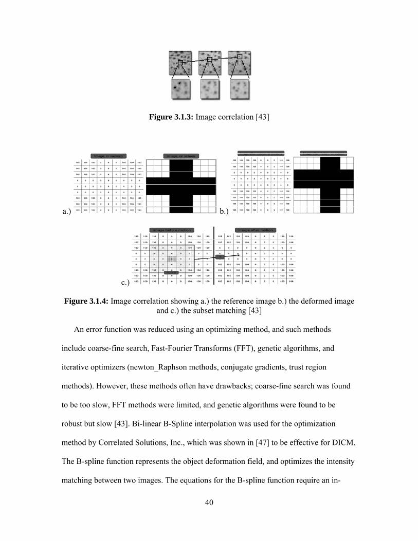
Figure 3.1.3: Image correlation [43]
a.) b.)
c.)
Figure 3.1.4: Image correlation showing a.) the reference image b.) the deformed image and c.) the subset matching [43]
An error function was reduced using an optimizing method, and such methods
include coarse-fine search, Fast-Fourier Transforms (FFT), genetic algorithms, and
iterative optimizers (newton_Raphson methods, conjugate gradients, trust region
methods). However, these methods often have drawbacks; coarse-fine search was found
to be too slow, FFT methods were limited, and genetic algorithms were found to be
robust but slow [43]. Bi-linear B-Spline interpolation was used for the optimization
method by Correlated Solutions, Inc., which was shown in [47] to be effective for DICM.
The B-spline function represents the object deformation field, and optimizes the intensity
matching between two images. The equations for the B-spline function require an in-
40

depth discussion, and the reader is referred to Ref. [47] for a description of these and the
equations for displacements and strains in DICM.
Vic3D data analysis software from Correlated Solutions was used in the present
research. In Vic3D, the displacements are calculated in the center of each subset. The
subset is defined as an nxn pixel window that surrounds a data point and represents a
strain window. During correlation, optimization equations are used to find out where the
window is in the deformed image, and the deformation is reported. The strains can then
be calculated from the deformation for each data point. The subsets are spaced by a user-
defined number of pixels, or step size. Subsets may overlap for a small stepsize, so that
the step size represents the increments, or steps, that the subset (strain window) is shifted
during correlation. A smaller step size yields more data points and also more computation
time. The displacement calculation is smoothed typically using a distortion order of 2 for
the data points in the subset. The in-plane displacement vector is calculated at every
subset center, and the strain is calculated from the triangle formed by three displacement
points. Due to variations inherent to experimental analysis, Vic3D uses a robust
correlation function, including a subset shape function from (similar to FEA) to define
the deformed subset. Displacements must be transformed into a useful coordinate system,
using calibration techniques [44].
As noted by Lagattu et. al. [45], measuring high strain gradients with DICM requires
a balance of parameters such as the speckle pattern, subset size, studied region size, data
point spacing, and measurable strain range. Once these parameters are accounted for,
DICM can be a useful tool to study high strain gradients such as those found around a
circular hole. As failure progresses, the redistribution of surface stress due to
41

delamination or fiber pullout can be observed. Full-field strains around the hole for the
entire loading range of a laminate can be compared for varied layups.
In the current study, a balance of parameters was found to be optimum during the
DICM data reduction. The final speckle pattern, shown in Fig. 3.1.2, worked well
because it was non-repetitive, isotropic, and high contrast. Speckle patterns with large
white or black areas did not correlate as well because larger dots required larger subsets.
Speckle patterns with a grey background also did not correlate well because of the lack of
contrast. The subset could not be smaller than the largest black or white region, or the
correlation function would have no variation in values to match between subsets. Fig.
3.1.5 shows different speckle patterns, and Fig. 3.1.6 shows the corresponding strain
profiles. The strain profiles in Fig. 3.1.6 are more consistent for the more isotropic and
higher contrast speckle patterns, as shown by the smoother lines. This trend in correlation
was shown for nearly all of the coupons tested, and thus the speckle pattern was found to
be one of the most important aspects of the test setup. Calibration was also clearly
important, and better correlation was found when the two cameras recorded the same
field of view. This could be achieved by locating dots in the speckle pattern, noting their
distance to the edges of the image, and matching the distance of the two camera images.
42
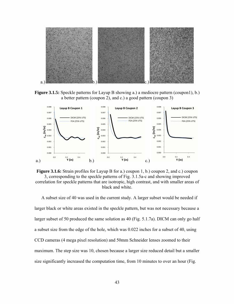
a.) b.) c.)
Figure 3.1.5: Speckle patterns for Layup B showing a.) a mediocre pattern (coupon1), b.) a better pattern (coupon 2), and c.) a good pattern (coupon 3)
a.) b.) c.)
0.000
0.001
0.002
0.003
0.004
0.005
0.006
0.007
0.008
0.0 0.2 0.4
ε xx(in
/in)
Y (in)
Layup B Coupon 1
DICM (25% UTS)
FEA (25% UTS)
0.000
0.001
0.002
0.003
0.004
0.005
0.006
0.007
0.008
0.0 0.2 0.4
ε xx(in
/in)
Y (in)
Layup B Coupon 2
DICM (25% UTS)FEA (25% UTS)
0.000
0.001
0.002
0.003
0.004
0.005
0.006
0.007
0.008
0.0 0.2 0.4ε x
x(in
/in)
Y (in)
Layup B Coupon 3
DICM (25% UTS)
FEA (25% UTS)
Figure 3.1.6: Strain profiles for Layup B for a.) coupon 1, b.) coupon 2, and c.) coupon 3, corresponding to the speckle patterns of Fig. 3.1.5a-c and showing improved
correlation for speckle patterns that are isotropic, high contrast, and with smaller areas of black and white.
A subset size of 40 was used in the current study. A larger subset would be needed if
larger black or white areas existed in the speckle pattern, but was not necessary because a
larger subset of 50 produced the same solution as 40 (Fig. 5.1.7a). DICM can only go half
a subset size from the edge of the hole, which was 0.022 inches for a subset of 40, using
CCD cameras (4 mega pixel resolution) and 50mm Schneider lenses zoomed to their
maximum. The step size was 10, chosen because a larger size reduced detail but a smaller
size significantly increased the computation time, from 10 minutes to over an hour (Fig.
43
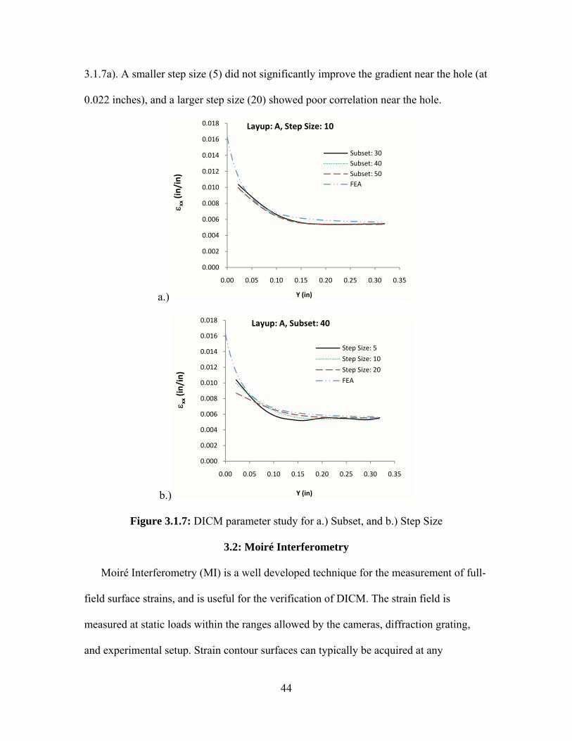
3.1.7a). A smaller step size (5) did not significantly improve the gradient near the hole (at
0.022 inches), and a larger step size (20) showed poor correlation near the hole.
a.)
0.000
0.002
0.004
0.006
0.008
0.010
0.012
0.014
0.016
0.018
0.00 0.05 0.10 0.15 0.20 0.25 0.30 0.35
ε xx(in
/in)
Y (in)
Layup: A, Step Size: 10
Subset: 30Subset: 40Subset: 50FEA
b.)
0.000
0.002
0.004
0.006
0.008
0.010
0.012
0.014
0.016
0.018
0.00 0.05 0.10 0.15 0.20 0.25 0.30 0.35
ε xx(in
/in)
Y (in)
Layup: A, Subset: 40
Step Size: 5
Step Size: 10
Step Size: 20
FEA
Figure 3.1.7: DICM parameter study for a.) Subset, and b.) Step Size
3.2: Moiré Interferometry
Moiré Interferometry (MI) is a well developed technique for the measurement of full-
field surface strains, and is useful for the verification of DICM. The strain field is
measured at static loads within the ranges allowed by the cameras, diffraction grating,
and experimental setup. Strain contour surfaces can typically be acquired at any
44
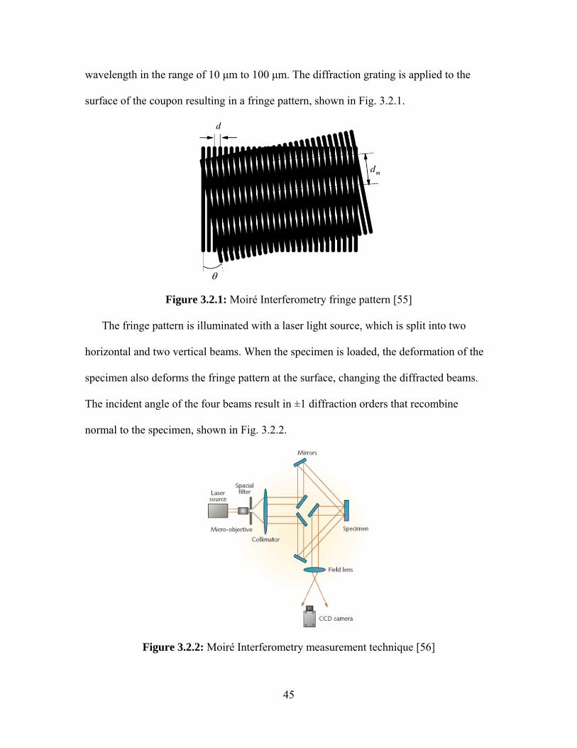
wavelength in the range of 10 μm to 100 μm. The diffraction grating is applied to the
surface of the coupon resulting in a fringe pattern, shown in Fig. 3.2.1.
Figure 3.2.1: Moiré Interferometry fringe pattern [55]
The fringe pattern is illuminated with a laser light source, which is split into two
horizontal and two vertical beams. When the specimen is loaded, the deformation of the
specimen also deforms the fringe pattern at the surface, changing the diffracted beams.
The incident angle of the four beams result in ±1 diffraction orders that recombine
normal to the specimen, shown in Fig. 3.2.2.
Figure 3.2.2: Moiré Interferometry measurement technique [56]
45

The recombined beams consist of interference patterns representing the deformation
of the coupon surface. The fringe patterns thus correspond to the in-plane displacements.
In order to measure longitudinal deformation, two horizontal beams are blocked using a
filter, and the two vertical beams interfere. This generates a vertical deformation field, or
V-Field. Similarly, in order to measure transverse deformation, two vertical beams are
blocked using a filter, and two horizontal beams interfere. This generates a horizontal
deformation field, or U-Field. The deformation fields can be related to in-plane strains
using [48, 49]
⎥⎦⎤⎡∂=
∂=
NU x1ε ⎢⎣ ∂∂ xfxx (3.2.1)
⎥⎦
⎤⎢⎡∂
=∂
=NV y1ε
⎣ ∂∂ yfyx (3.2.2)
⎥⎦
⎤⎢⎡ ∂
+∂
=∂
+∂
=NNVU yx1γ (3.2.3)
⎣ ∂∂∂∂ xyfyyxy
where f is the virtual grating frequency, Nx is the horizontal fringe order, and Ny is the
vertical fringe order. The fringe orders are retrieved from the unwrapped phase
distribution of the corresponding Moiré interferometric fringe pattern.
MI was used to measure deformation in composite multi-span beam shear specimens
in [50]. Analysis of composite beams under 5-point and 3-point flexure showed free-edge
effects produced shears on the edge of the beams, and that MI performed well for whole-
field strain analysis of composites. A fourier-transform method for analyzing fringe
patterns of Moiré Interferometry was performed by [51]. Surface strain measurements of
46

carbon-fiber/PEEK composite laminates were successfully achieved up to 37.9% the
theoretical limit of the fringe pattern.
Moiré and DICM are compared in Chapter 5. While both accurately measure strains
in the elastic region of composite laminates, Moiré was not able to obtain strains in the
damaged region. DICM has the advantage of continuous measurement and correlation,
while Moiré generally has higher accuracy, and can measure strains from 0.002 to 2%.
DICM has limits of measurement at extremely low strains due to the limit of the CCD
cameras, as will be shown in Chapter 5. However, Moiré can only take measurements at
static loads, and precautions must be taken to minimize vibrations from the equipment
and the building. Thus, DICM is more useful for measuring the surface strain of many
laminates over their entire load range.
47
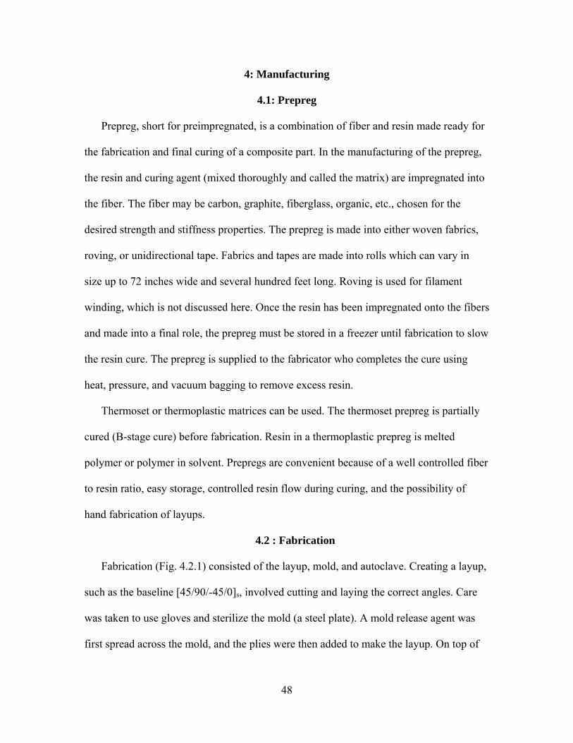
4: Manufacturing
4.1: Prepreg
Prepreg, short for preimpregnated, is a combination of fiber and resin made ready for
the fabrication and final curing of a composite part. In the manufacturing of the prepreg,
the resin and curing agent (mixed thoroughly and called the matrix) are impregnated into
the fiber. The fiber may be carbon, graphite, fiberglass, organic, etc., chosen for the
desired strength and stiffness properties. The prepreg is made into either woven fabrics,
roving, or unidirectional tape. Fabrics and tapes are made into rolls which can vary in
size up to 72 inches wide and several hundred feet long. Roving is used for filament
winding, which is not discussed here. Once the resin has been impregnated onto the fibers
and made into a final role, the prepreg must be stored in a freezer until fabrication to slow
the resin cure. The prepreg is supplied to the fabricator who completes the cure using
heat, pressure, and vacuum bagging to remove excess resin.
Thermoset or thermoplastic matrices can be used. The thermoset prepreg is partially
cured (B-stage cure) before fabrication. Resin in a thermoplastic prepreg is melted
polymer or polymer in solvent. Prepregs are convenient because of a well controlled fiber
to resin ratio, easy storage, controlled resin flow during curing, and the possibility of
hand fabrication of layups.
4.2 : Fabrication
Fabrication (Fig. 4.2.1) consisted of the layup, mold, and autoclave. Creating a layup,
such as the baseline [45/90/-45/0]s, involved cutting and laying the correct angles. Care
was taken to use gloves and sterilize the mold (a steel plate). A mold release agent was
first spread across the mold, and the plies were then added to make the layup. On top of
48

the layup, peel ply was added which allowed the resin to bleed through during cure, and
did not stick to the composite. Breather cloth was put on top, and the vacuum nozzle was
placed on top of this. Butyl tape was placed in a rectangle surrounding the part, and
vacuum bagging material was sealed on top of everything, with a slit for the vacuum
tube.
Figure 4.2.1: Fabrication setup
The autoclave was set to a specific cure cycle, as prescribed in literature. This cure
cycle starts with a ramp period, in which temperature and pressure were increased at a
constant rate. The part was soaked at a specific temperature and pressure for a given time,
followed by a ramp down period. For the current study, open-hole tension coupons were
fabricated from 16 plies of carbon/epoxy prepreg (T600/125-33). All coupons were
autoclave cured at 350 ºF and 90 psig. After a 10 minute ramp period, the coupons were
then soaked at this temperature and pressure for 45 minutes and then slowly cooled
(under a constant pressure of 90 psig) for an additional 45 minutes. Coupons were
machined from fabricated plaques using a waterjet system and an aerospace quality
abrasive mixture. The holes were drilled with a drill press, as would be encountered in
industry. The effect of this process is discussed in Chapter 5.
49

5: Results
5.1: Introduction
Linear finite element analysis was applied to kt- and FPF-optimization methods to
tailor non-traditional laminates in open-hole tension (Chapter 2). Some layups were not
fabricated because they were either repetitive or irrelevant (Section 2.4). The final eleven
layups, shown in Table 5.1.1, were fabricated according to the techniques explained in
Chapter 4 and the dimensions given in Appendix B. The coupons were speckled and
loaded in an MTS load frame (10 kip load cell) during which DICM surface strain
measurements (Chapter 3) were taken.
Table 5.1.1: Fabricated layups8 Designation Layup Method Description
BL [(45/90/-45/0)2]s Quasi-isotropic Baseline A [(54/90/-54/0)2]s kt Vary 45º B [(45/51/-45/0)2]s kt Vary 90º C [(45/0/-45/90)2]s Stacking sequence Vary Order 1 D [(45/90/-45/57)2]s kt Vary 0º E [(54/54/-54/0)2]s FPF Vary 45º & 90º F [(45/-45/90/0)2]s Stacking sequence Vary Order 2 G [(21/90/-21/0)2]s FPF Vary 45º H [(45/0/-45/0)2]s FPF Vary 90º I [(±45)4]s Failure mode Shear failure J [0]16 Failure mode Uniaxial failure
DICM has been used by others to quantitatively and qualitatively characterize surface
strain. DICM can be used to observe the strain concentration near a hole, as shown in Fig.
5.1.1, where the strain contours of a composite laminate (5.1.1.a) and a wood specimen
(5.1.1b) are given. Fig. 5.1.2 shows the strain profile along the net section of a composite
laminate in fatigue. The strain contours can be used to understand strain patterns around
the hole, and the strain profile can be used to quantify those observations.
8 The layups are all balanced (the same number of +/- plies on either side of the center line).
50

a.) b.)
Figure. 5.1.1: a.) Von Mises strain map measured by DICM around a 5 mm hole on a
thermoplastic matrix composite, σapplied=67% σfailure (vertical loading) [45] b.) Transverse displacement (mm x 10-3) contour plots by DICM near a bolt (vertical load) [52].
Figure 5.1.2: Longitudinal strain versus distance from the hole at the net section of a fatigued [0/±45/90]2s graphite/PEEk sample; maximum load=75% of the ultimate static
load [46].
Experimental measurement of FPF can be a difficult task. There is no generally
accepted experimental method for determining FPF, such as the 2% offset rule for yield
in some metals. The idealized load-strain curve displays several piecewise linear sections
separated by “knees” that correspond to the kth ply failure (Fig. 5.1.3). In reality, the
changes in stiffness are often more subtle for first ply failure (Fig. 5.1.4), and may be
51

nonlinear for subsequent ply failures. In the World Wide Failure Exercise [1], results for
initial failure were poor because of a shortage of reliable experimental data, and because
of discrepancies between experimental and theoretical definitions of initial failure.
Experimental analysis of FPF is further complicated by the inherent variations in
manufacturing. Stress-strain plots for coupons of the same layup will vary as damage
progresses, as shown by the diverging data points of Fig. 5.1.4. These issues will be
discussed, and experimental methods will be suggested, in Section 5.4.
Figure 5.1.3: Idealized load-strain curve for uniaxially loaded laminate showing multiple ply failures leading up to ultimate laminate failure. [26]
Figure 5.1.4: Comparison of predicted and measured stress-strain response of [0/±45/90]s glass/epoxy laminate. [53]
52
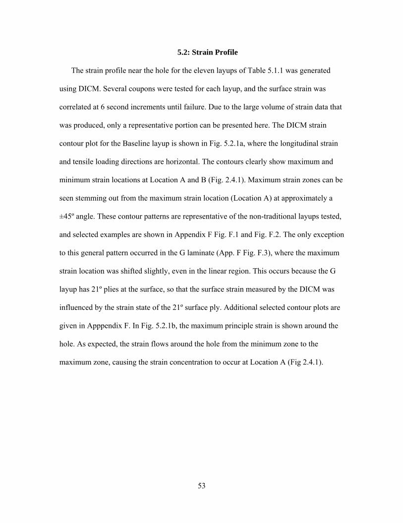
5.2: Strain Profile
The strain profile near the hole for the eleven layups of Table 5.1.1 was generated
using DICM. Several coupons were tested for each layup, and the surface strain was
correlated at 6 second increments until failure. Due to the large volume of strain data that
was produced, only a representative portion can be presented here. The DICM strain
contour plot for the Baseline layup is shown in Fig. 5.2.1a, where the longitudinal strain
and tensile loading directions are horizontal. The contours clearly show maximum and
minimum strain locations at Location A and B (Fig. 2.4.1). Maximum strain zones can be
seen stemming out from the maximum strain location (Location A) at approximately a
±45º angle. These contour patterns are representative of the non-traditional layups tested,
and selected examples are shown in Appendix F Fig. F.1 and Fig. F.2. The only exception
to this general pattern occurred in the G laminate (App. F Fig. F.3), where the maximum
strain location was shifted slightly, even in the linear region. This occurs because the G
layup has 21º plies at the surface, so that the surface strain measured by the DICM was
influenced by the strain state of the 21º surface ply. Additional selected contour plots are
given in Apppendix F. In Fig. 5.2.1b, the maximum principle strain is shown around the
hole. As expected, the strain flows around the hole from the minimum zone to the
maximum zone, causing the strain concentration to occur at Location A (Fig 2.4.1).
53

a.)
b.)
Figure 5.2.1: a.) Longitudinal strain DICM contours and b.) Principle strain vectors for the Baseline laminate at 19 Ksi (26% UTS), where tensile loading is horizontal.
Moiré Interferometry deformation contours are shown in Fig. 5.2.2 for the Baseline
layup. For Moiré interfermetry, lines closer together indicate high deformation zones and
correspond to the high strain zones of DICM shown in Fig 5.2.1. Thus, the high strain
zones at the top and bottom of the hole and the low strain zones at the sides of the hole of
Fig. 5.2.1 from DICM correspond well to the high and low deformation zones of Moiré
Interferometry shown in Fig. 5.2.2. However, the quality of contours at the top and
bottom of the hole in Fig. 5.2.2 degrades, perhaps due to damage introduced by drilling
the hole. As noted by [10], the drilling process may introduce delimitation, which would
54
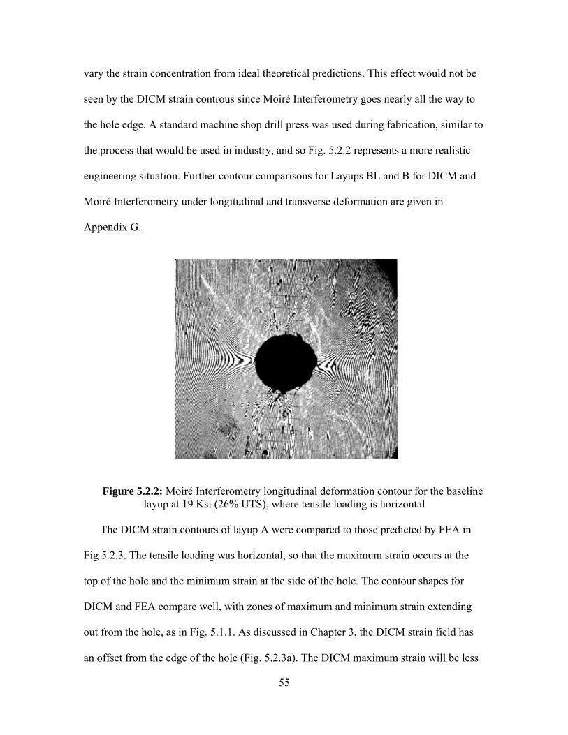
vary the strain concentration from ideal theoretical predictions. This effect would not be
seen by the DICM strain controus since Moiré Interferometry goes nearly all the way to
the hole edge. A standard machine shop drill press was used during fabrication, similar to
the process that would be used in industry, and so Fig. 5.2.2 represents a more realistic
engineering situation. Further contour comparisons for Layups BL and B for DICM and
Moiré Interferometry under longitudinal and transverse deformation are given in
Appendix G.
Figure 5.2.2: Moiré Interferometry longitudinal deformation contour for the baseline
layup at 19 Ksi (26% UTS), where tensile loading is horizontal The DICM strain contours of layup A were compared to those predicted by FEA in
Fig 5.2.3. The tensile loading was horizontal, so that the maximum strain occurs at the
top of the hole and the minimum strain at the side of the hole. The contour shapes for
DICM and FEA compare well, with zones of maximum and minimum strain extending
out from the hole, as in Fig. 5.1.1. As discussed in Chapter 3, the DICM strain field has
an offset from the edge of the hole (Fig. 5.2.3a). The DICM maximum strain will be less
55

than that predicted by FEA because the DICM strain field does not go to the edge of the
hole. The plotted strain range from the DICM contours was used for the FEA contours
(Fig. 5.2.3.b). The gray areas near the top and side of the hole in Fig. 5.2.3.b represent
strains above or below this range. The FEA gray area peaks should correspond to the
DICM maximum and minimum strain locations. This is approximately true for the
maximum strain, with FEA peak and DICM offset locations of 0.022 and 0.024 inches
from the hole. However, the locations do not compare as well at the minimum strain with
FEA peak and DICM offset locations of 0.056 and 0.026 inches from the hole. This
discrepancy reveals that DICM correlates well with linear FEA for higher strains but less
well for very low strains, as would be seen at the minimum strain zone of Location B
(Fig. 2.4.1).
a.) b.)
Figure 5.2.3: Strain contours for layup A at 38 Ksi (53% UTS) in a strain range of 0.00117 in/in to 0.0121 in/in for a.) DICM and b.) 2D linear FEA. The gray band for b.)
near the top and side of the hole represents strains above and below the strain range.
Fig. 5.2.4 shows the development of longitudinal, shear, and transverse strain
profiles along the net-section of selected layups, at loads of (or near) 25%, 50%, 75%,
and 90% UTS. As expected, the strain is maximum at the hole due to the strain
concentration induced by the absence of material. The transverse strain is negative due to
the Poisson effect. These graphs represent the general trend for the strain profiles of the
56

non-traditional layups tested, and the corresponding strain ranges. The trends are also
illustrated by the contour plots of App. F., F.1-F.6.
a.) b.)
0
0.005
0.01
0.015
0.02
0.025
0.03
0.035
0 0.1 0.2 0.3 0.4 0.5
ε xx(in
/in)
Y (in)
90%
74%
49%
24%
% UTS
0
0.002
0.004
0.006
0.008
0.01
0.012
0.014
0.016
0.018
0 0.2 0.4 0.6
γ xy(in
/in)
Y (in)
87%
76%
49%
26%
% UTS
c.) -0.008
-0.007
-0.006
-0.005
-0.004
-0.003
-0.002
-0.001
0
0 0.2 0.4 0.6ε y
y(in
/in)
Y (in)
90%
75%
50%
25%
% UTS
Figure 5.2.4: Strain vs. Y distance from the hole using DICM for a.) longitudinal
strain: layup D, b.) shear strain: layup B, and c.) transverse strain: layup A.
The longitudinal and shear strain profiles are compared in Fig. 5.2.5 for selected
layups. The general trend remains consistent for all the layups, with the maximum at the
hole and a decline in strain for the rest of the net section. Variations can be seen in
magnitude of the maximum strain and the existence of “peaks” and “valleys” along the
curve. The variation in the maximum strain is due to the specific layup’s strain response
to the applied load (90% UTS in Fig. 5.2.5), and the peaks and valleys are due to a
57

combination of factors including the layup, load, speckle pattern, and coupon
irregularities introduced during fabrication. From the magnitude of the maximum strains
near the hole in Figs. 5.2.4 and 5.2.5, it seems reasonable that failure will be primarily
dependent on the longitudinal strain and shear strain. Indeed, this is supported by the
Maximum Strain Criterion, in which first and second ply failure modes are always either
due to the longitudinal strain or the shear strain, which will be discussed further in
Section 5.3 and 5.4.
a.) b.)
0
0.005
0.01
0.015
0.02
0.025
0.03
0.035
0.04
0 0.2 0.4 0.6
ε xx(in
/in)
Y (in)
A-1-4
B-1-4
C-1-4
D-1-4
0
0.002
0.004
0.006
0.008
0.01
0.012
0.014
0.016
0.018
0 0.2 0.4 0.6
γ xy(in
/in)
Y (in)
A-1-4
B-1-4
C-1-4
D-1-4
Figure 5.2.5: Strain vs. Y distance from the hole plots of selected coupons at 90% UTS for a.) longitudinal strain and b.) shear strain.
The stress-strain curves are plotted at Location A (Fig. 2.4.1) for selected layups in
Fig. 5.2.6. The curves are clearly non-linear, indicating damage at the hole. “Knee”
points represent ply failure and can be seen throughout the curves, which will be
discussed in Section 5.3 and 5.4. The position of the curves relative to one another may
change for longitudinal or shear stiffness, as shown by the layup A and B coupons. As
damage progresses, some curves may soften more than others, as seen by comparing the
A and B coupons, as well as the BL and D coupons. All the non-traditional laminates
58

showed decreasing stiffness as damage progressed. Figs. 5.2.4-5.2.6 demonstrate the
comparisons that can be generated using DICM.
a.) b.)
0
10
20
30
40
50
60
70
80
0.00 0.01 0.02 0.03 0.04
σ x(Ksi)
εxx (in/in)
BL-1-4A-1-4B-1-4D-1-4
0
10
20
30
40
50
60
70
80
0.000 0.005 0.010 0.015 0.020
σ x(k
si)
γxy (in/in)
BL-1-4A-1-4B-1-4D-1-4
Figure 5.2.6: Stress vs. strain plots of selected coupons for a.) longitudinal strain and b.) shear strain.
To quantitatively compare DICM to the 2D FEA model, the axial strain was plotted
as a function of the distance from the hole (normal to the loading direction) as shown in
Fig. 5.2.7. DICM is not valid at the edge of the specimen (Fig. 5.2.1), so the DICM data
in Fig. 5.2.7 begins at 0.022 in from the hole. For mid-range loading (10 to 50% UTS) the
DICM solution compares reasonably well to linear FEA. The coupon used in Fig. 5.2.7
had a good speckle pattern (isotropic, high contrast, Fig. 3.1.5c), with camera images set
closely to each other to improve calibration and correlation. For coupons with the speckle
patterns of Fig. 3.1.5a-b (about two-thirds of the coupons tested), correlation was found
to be reasonably good for 25 to 50% UTS. For all the coupons at high loads (90% UTS),
non-linear effects become large, and the comparison deteriorates because the 2D FEA is
linear. At low loads (<25% UTS), the comparison again deteriorates because DICM
correlates poorly for low strains, as shown in Fig. 5.2.3. The DICM strain profile begins
to decline near the hole for 90% UTS. This is due to the shifting of the strain
concentration to the left under high damage, as shown in Fig. 5.2.8. This shift can be seen
59

to occur due to the ply splitting along the 45º angle during damage progression, as shown
by Fig. 5.2.9. The highest strain occurred at the crack, shown by Strain Profile 1 of Fig.
5.2.9. As the strain profile locations were moved away from the crack and away from
Location A, the strain profiles decreased as shown by Strain Profiles 2 and 3.
0.00
0.01
0.02
0.03
0.04
0.05
0.00 0.05 0.10 0.15 0.20 0.25 0.30 0.35 0.40 0.45 0.50
ε xx(in
/in)
Y (in)
DICM
FEA
90% UTS
50% UTS
25% UTS
10% UTS
Figure 5.2.7: Longitudinal strain of layup A as a function of distance from the hole for DICM and 2D FEA
a.) b.) Figure 5.2.8: Longitudinal strain contours for layup A at a.) 90% UTS and b.) 98% UTS
showing the maximum strain at the left of the net-section during high damage
60

a.)
b.)
0.00
0.01
0.02
0.03
0.04
0.05
0.06
0.00 0.10 0.20 0.30 0.40
ε xx(in
/in)
Y (in)
DICM Strain Profile 1
DICM Strain Profile 2
DICM Strain Profile 3
FEA Strain Profile 2
Figure 5.2.9: a.) Diagram showing the crack and the location of the strain profiles, and b.) strain profiles for Layup A at 90% UTS
The shift of the strain concentration in Fig.’s 5.2.7 -5.2.9 was unique to the damage of
this coupon, as shown Fig. 5.2.10a in which the strain profile for another Layup A
coupon does not decline near the hole. This illustrates the variability that can occur
during damage progression due to coupon irregularities introduced during fabrication.
Fig. 5.2.10b-d shows the strain profile along the net section of several other layups at
90% UTS, compared to linear FEA. This shows that the DICM curve is consistently
higher than the linear FEA curve. This is expected, since the modulus should decrease
during softening causing the strain to increase for the same applied stress.
61
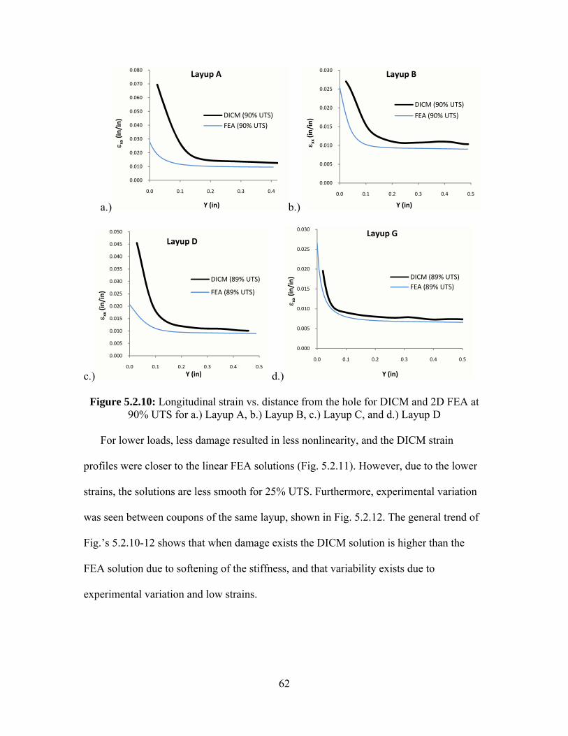
a.) b.)
0.000
0.010
0.020
0.030
0.040
0.050
0.060
0.070
0.080
0.0 0.1 0.2 0.3 0.4
ε xx(in
/in)
Y (in)
Layup A
DICM (90% UTS)FEA (90% UTS)
0.000
0.005
0.010
0.015
0.020
0.025
0.030
0.0 0.1 0.2 0.3 0.4 0.5
ε xx(in
/in)
Y (in)
Layup B
DICM (90% UTS)
FEA (90% UTS)
c.) d.)
0.000
0.005
0.010
0.015
0.020
0.025
0.030
0.035
0.040
0.045
0.050
0.0 0.1 0.2 0.3 0.4 0.5
ε xx(in
/in)
Y (in)
Layup D
DICM (89% UTS)
FEA (89% UTS)
0.000
0.005
0.010
0.015
0.020
0.025
0.030
0.0 0.1 0.2 0.3 0.4 0.5
ε xx(in
/in)
Y (in)
Layup G
DICM (89% UTS)FEA (89% UTS)
Figure 5.2.10: Longitudinal strain vs. distance from the hole for DICM and 2D FEA at 90% UTS for a.) Layup A, b.) Layup B, c.) Layup C, and d.) Layup D
For lower loads, less damage resulted in less nonlinearity, and the DICM strain
profiles were closer to the linear FEA solutions (Fig. 5.2.11). However, due to the lower
strains, the solutions are less smooth for 25% UTS. Furthermore, experimental variation
was seen between coupons of the same layup, shown in Fig. 5.2.12. The general trend of
Fig.’s 5.2.10-12 shows that when damage exists the DICM solution is higher than the
FEA solution due to softening of the stiffness, and that variability exists due to
experimental variation and low strains.
62
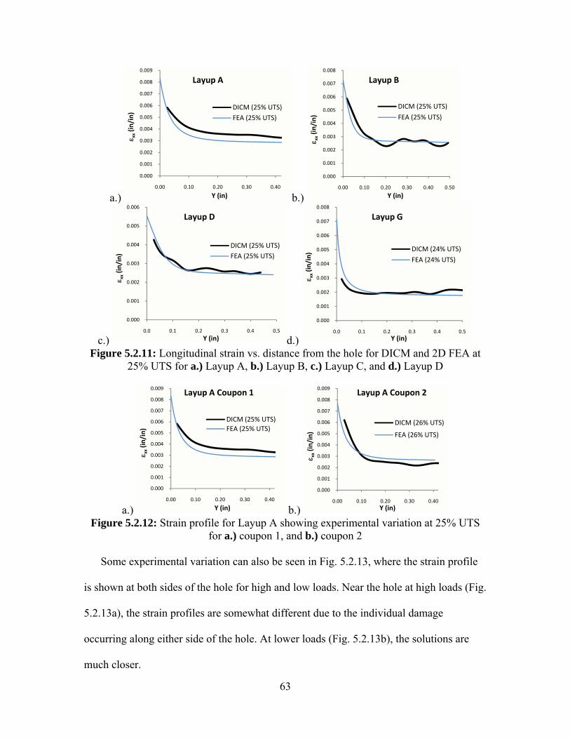
a.) b.)
0.000
0.001
0.002
0.003
0.004
0.005
0.006
0.007
0.008
0.009
0.00 0.10 0.20 0.30 0.40
ε xx(in
/in)
Y (in)
Layup A
DICM (25% UTS)FEA (25% UTS)
0.000
0.001
0.002
0.003
0.004
0.005
0.006
0.007
0.008
0.00 0.10 0.20 0.30 0.40 0.50
ε xx(in
/in)
Y (in)
Layup B
DICM (25% UTS)
FEA (25% UTS)
c.) d.)
0.000
0.001
0.002
0.003
0.004
0.005
0.006
0.0 0.1 0.2 0.3 0.4 0.5
ε xx(in
/in)
Y (in)
Layup D
DICM (25% UTS)FEA (25% UTS)
0.000
0.001
0.002
0.003
0.004
0.005
0.006
0.007
0.008
0.0 0.1 0.2 0.3 0.4 0.5
ε xx(in
/in)
Y (in)
Layup G
DICM (24% UTS)
FEA (24% UTS)
Figure 5.2.11: Longitudinal strain vs. distance from the hole for DICM and 2D FEA at 25% UTS for a.) Layup A, b.) Layup B, c.) Layup C, and d.) Layup D
a.) b.)
0.000
0.001
0.002
0.003
0.004
0.005
0.006
0.007
0.008
0.009
0.00 0.10 0.20 0.30 0.40
ε xx(in
/in)
Y (in)
Layup A Coupon 1
DICM (25% UTS)FEA (25% UTS)
0.000
0.001
0.002
0.003
0.004
0.005
0.006
0.007
0.008
0.009
0.00 0.10 0.20 0.30 0.40
ε xx(in
/in)
Y (in)
Layup A Coupon 2
DICM (26% UTS)
FEA (26% UTS)
Figure 5.2.12: Strain profile for Layup A showing experimental variation at 25% UTS for a.) coupon 1, and b.) coupon 2
Some experimental variation can also be seen in Fig. 5.2.13, where the strain profile
is shown at both sides of the hole for high and low loads. Near the hole at high loads (Fig.
5.2.13a), the strain profiles are somewhat different due to the individual damage
occurring along either side of the hole. At lower loads (Fig. 5.2.13b), the solutions are
much closer.
63
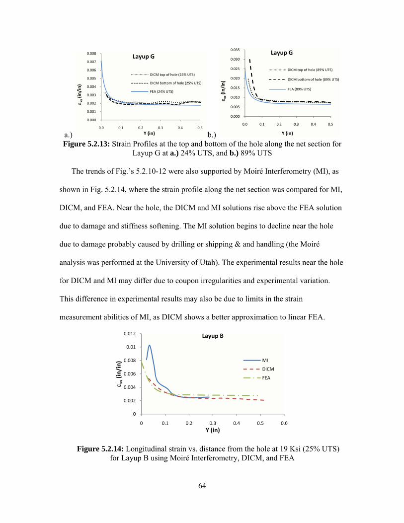
a.) b.)
0.000
0.001
0.002
0.003
0.004
0.005
0.006
0.007
0.008
0.0 0.1 0.2 0.3 0.4 0.5
ε xx(in
/in)
Y (in)
Layup G
DICM top of hole (24% UTS)
DICM bottom of hole (25% UTS)
FEA (24% UTS)
0.000
0.005
0.010
0.015
0.020
0.025
0.030
0.035
0.0 0.1 0.2 0.3 0.4 0.5
ε xx(in
/in)
Y (in)
Layup G
DICM top of hole (89% UTS)
DICM bottom of hole (89% UTS)
FEA (89% UTS)
Figure 5.2.13: Strain Profiles at the top and bottom of the hole along the net section for Layup G at a.) 24% UTS, and b.) 89% UTS
The trends of Fig.’s 5.2.10-12 were also supported by Moiré Interferometry (MI), as
shown in Fig. 5.2.14, where the strain profile along the net section was compared for MI,
DICM, and FEA. Near the hole, the DICM and MI solutions rise above the FEA solution
due to damage and stiffness softening. The MI solution begins to decline near the hole
due to damage probably caused by drilling or shipping & and handling (the Moiré
analysis was performed at the University of Utah). The experimental results near the hole
for DICM and MI may differ due to coupon irregularities and experimental variation.
This difference in experimental results may also be due to limits in the strain
measurement abilities of MI, as DICM shows a better approximation to linear FEA.
0
0.002
0.004
0.006
0.008
0.01
0.012
0 0.1 0.2 0.3 0.4 0.5 0.6
ε xx(in
/in)
Y (in)
Layup B
MI
DICM
FEA
Figure 5.2.14: Longitudinal strain vs. distance from the hole at 19 Ksi (25% UTS) for Layup B using Moiré Interferometry, DICM, and FEA
64
The experimental and theoretical strain concentrations were compared in Fig. 5.2.15
using DICM and linear 2D FEA, respectively. The experimental kt was found as the slope
of the εmax vs. εnom DICM plot in the linear region, with a correction factor applied as
explained in Section 2.2. To obtain an accurate comparison, the kt’s from the FEA were
compared to DICM at the DICM offset location, instead of Location A from Fig. 2.4.1. A
representative offset of 0.022 inches was used, due to the fact that the same or nearly the
same subset was used for the over 50 coupons tested resulting in approximately the same
offset for all the coupons. The DICM nominal strain was not a true nominal strain due to
the limits of the measureable area of the DICM camera. The DICM nominal strain
location was taken at (0.5 in, 0.375 in), as was the FEA nominal strain to obtain an
accurate comparison. This location was taken in order to avoid the minimum strain zone
stemming from Location B (Fig. 2.4.1), and also to avoid free-edge effects, and thus be as
close to the true experimental nominal strain as possible. The DICM- and FEA-predicted
kt’s did not compare well, due to the experimental variation near the hole shown by Fig.’s
5.2.10-5.2.13. Fig. 5.2.16 shows the difference between the adjusted DICM location kt,
used in Fig. 5.2.15, and the original Location A based kt, used in Chapter 2 . The large
variation in kt between these locations is due to the large strain gradient that exists near
the hole. This strain gradient, along with the experimental variation of Figs. 5.2.10-
5.2.12, explains the variation in experimental and theoretical results of Fig. 5.2.15. This
variation suggests that DICM can only be used as an indication of the strain concentration
near the hole.
65

0.00
0.50
1.00
1.50
2.00
2.50
3.00
BL A B C D E F G H I J
k t
DICM FEA
Figure 5.2.15: Comparison of experimental (DICM) and theoretical (2D linear FEA) results for the strain concentration, kt, at the DICM location (εmax at 0.022 inches from the
hole and εmin at (0.5, 0.375) inches from the coupon center)
Figure 5.2.16: Comparison of the kt from the DICM location (εmax at 0.022 inches from the hole and εmin at (0.5, 0.375) inches from the coupon center) to the kt from Location A
(εmax at Location A, Fig. 2.4.1, and εmin at (4, 0) from the coupon center )
0.00
1.00
2.00
3.00
4.00
5.00
6.00
BL A B C D E F G H I J
k t
FEA (DICM location)
FEA (Location A)
Fig. 5.2.17 compares the modulus calculated using DICM and FEA at the (0.5, 0.375)
nominal location. The modulus was calculated using the nominal strain and the applied
stress. As mentioned for Fig. 5.2.15, the nominal location was taken to avoid maximum
strain zones and be as close to the true nominal as the DICM strain field would allow.
66

Fig. 5.2.17 shows that the theoretical modulus was near but consistently higher than the
DICM modulus. This may be due to through-the-thickness effects caused by the
interlaminar interaction between plies of varying angles, not accounted for in 2D FEA.
Fig. 5.2.17 shows that a reasonable experimental and theoretical comparison exists for
the modulus in the linear region.
0
5
10
15
20
BL A B C D E F G H I J
E x(M
si)
DICM
FEA
Figure 5.2.17: Comparison of experimental (DICM) and theoretical (FEA) results for the longitudinal modulus, Ex
67

5.3: Failure Modes
This section discusses Layups I and J, which were [(±45)4]s and [0]16, respectively
(Table 5.1.1). These layups were fabricated to study the corresponding shear and
longitudinal failure modes, in order to better understand failure in the non-traditional
laminates. In Fig. 5.3.1, the uniaxial applied stress-longitudinal strain curve slopes
upward after the proportional limit, indicating an increase in stiffness after damage
initiation. This increase in stiffness is unique to the uniaxial layup, as the stiffness
decreases near the hole during damage progression for common hard layups (those with
high numbers of 0º plies), noted by References [2] and [22]. The decrease in stiffness
noted in the literature was supported in the current study by the stress-strain curve of the
hard laminate H, shown at the end of Appendix H.1. The stiffness increases for Layup J
is due to the physical nature of the uniaxial layup, where the stress concentration is
redistributed due to longitudinal matrix splitting. This stress redistribution is shown in
Fig. 5.3.2, where the slope equals the strain concentration (without the correction factor
of Section 2.2 applied, since the variable of interest is only the change in slope). The
slope of Fig 5.3.2 decreases at the load where the stiffness of Fig. 5.3.1 increases (47.4
ksi), indicating that stress redistribution has occurred. This stress redistribution causes an
increase in stiffness in the uniaxial layup due to the stress concentration being effectively
“cut-off”, and the coupon being divided into three sections, as shown in Fig. 5.3.3d. This
division is suppressed in most hard laminates due to secondary load bearing plies (such as
the ±45º plies of Layup H), which cause the stiffness to decrease after stress
redistribution. The decrease in stiffness after stress redistribution is much less in hard
68

laminates (Layup H), than in less hard laminates (Layup D), as would be expected. This
trend can be seen in App. H and will be discussed in Section 5.4.
Figure 5.3.1: Stress vs. longitudinal strain for a uniaxial coupon (Layup J) showing an
increase in stiffness after damage initation (at Location A, Fig. 2.4.1)
0
10
20
30
40
50
60
70
80
0.000 0.001 0.002 0.003 0.004 0.005 0.006 0.007
σ x(K
si)
εxx (in/in)
Damage initiation at 47.4 Ksi
0.000
0.001
0.002
0.003
0.004
0.005
0.006
0.007
0.000 0.001 0.002 0.003 0.004 0.005 0.006
ε xx,
max
(in/in
)
εxx,nom (in/in)
Strain concentration decrease at 47.4 Ksi
Figure 5.3.2: Maximum vs. nominal strain for layup J (uniaxial), indicating a stress redistribution where the slope (representing the strain concentration) decreases, corresponding to an increase in stiffness in Fig. 5.3.1 (at Location A, Fig 2.4.1)
69
FPF is located at the first “knee” point of the stress vs. strain curve (Fig. 5.1.3), and
corresponds to the proportional limit of this curve [26]. This knee was found for the
traditional [0/±45/90]s laminate in Ref. [53], and occurred in the 90º plies. The 90º ply is
expected to fail first because the matrix resists the applied stress and not the fibers,
causing FPF due to the transverse matrix failure mode. For open-hole tension, this failure
mode is expected to occur at Location A (Fig. 2.4.1) where the maximum longitudinal
strain occurs. However, the 90º plies were altered for some of the non-traditional
laminates (Table 5.1.1), and no 90º plies existed in the failure mode laminates (Layups I
and J), so FPF could theoretically occur anywhere along the circumference of the hole,
and due to any failure mode (shear, transverse, or longitudinal) for these layups. For the
non-traditional layups, the question of where FPF occurs will be resolved in Section 5.4.
For the failure mode layups, this question is resolved in the following discussion.
Wherever FPF occurs, it should correspond to a slope change in the experimental
stress-strain curve at this location because the resulting damage should soften (reduce)
the stiffness. Depending on the failure-mode (longitudinal, transverse, or shear), this
slope change may be best observed using the stress-longitudinal strain, stress-transverse
strain, or stress-shear strain curve. FPF cannot be observed experimentally except under
CT scanning, which was not available for the current study, but will be examined by
Kothidar [42]. Thus, the method in the current study for locating FPF was to locate the
change in stiffness of the stress-strain curve (the “knee” point of Fig. 5.1.3), and compare
this to linear FEA and failure criteria.
The Maximum Strain Criterion predicts a longitudinal failure mode for the uniaxial
Layup J at Location A, which would indicate fiber breakage and thus catastrophic failure.
70

This failure mode would suggest that either FPF equals UTS for Layup J, or that FPF is
occurring somewhere else in the coupon. For Layup J, Fig. 5.3.3 shows that high
transverse and shear strains develop at the hole edge at approximately ±60º from the
longitudinal direction, defined now as Location C (Fig. 5.3.3.c). Since the longitudinal
failure index at Location A was found to be small (App. A Table A.5), and since the
transverse strains at Location C are much higher than usual (Fig. 5.3.3), it is reasonable to
suggest that failure may initiate at Location C instead of Location A for Layup J.
a.) εxx,max = 0.00894 b.) εyy, max = 0.0245
c.) γxy, max = 0.0471 d.) Failure
Location C
Figure 5.3.3: Strain contours at 90% UTS for Layup J showing a.) longitudinal strain, b.) transverse strain and, c.) shear strain. Image “d” shows the uniaxial coupon failed due to
matrix splitting at the sides of the hole.
The experimental DICM strain contours qualitatively compare well with the
theoretical linear FEA strain contours for Layup J at 25% UTS (Fig. 5.3.4) at Location A
71

and Location C. Thus, the FPF from the experimental stress-strain curve (the “knee”
point of Fig. 5.1.3), should compare well to linear FEA and failure criteria.
a.)
b.)
c.) Figure 5.3.4: DICM (left image) and FEA (right image) strain contours at 25% UTS
for a.) longitudinal strain, b.) transverse strain, and c.) shear strain
72

Using Location C and comparing experiment to theory, good correlation was found
for FPF (Fig. 5.3.5a). The Maximum Strain prediction for FPF in Fig. 5.3.5a is shown by
a horizontal line indicating the stress, and text indicating the failure ply (45º) and failure
mode (shear, 12). Using the second highest failure mode (transverse) for second ply
failure (SPF)9, and comparing this to the second proportional limit in the shear,
transverse, and longitudinal stress-strain curves (Fig. 5.3.5a-c), a strong correlation was
also found. These results indicate that if the stress-strain curve is close to linear, then
linear FEA and the Maximum Strain Criteria can predict FPF and SPF. However, SPF
was not pursued in this paper due to its dependence on nonlinear damage. Furthermore,
as shown by Refs. [14] and [15], after damage initiation strain is no longer constant
through-the-thickness, which would affect the surface strain measurements of DICM.
This affect would need to be quantified using a nonlinear 3D FEA model before SPF
could be understood, and is left for future research.
From these comparisons it is suggested that FPF in uniaxial coupons with center
holes occurs due to the shear failure-mode at Location C, and that final failure is
primarily due to matrix splitting at the sides of the hole (Fig. 5.3.3d). The longitudinal
(fiber failure) mode was predicted to occur last, but the catastrophic failure that normally
accompanies this failure mode was not seen. Thus, shear and transverse failure modes
may have caused the matrix splitting that lead to final failure. However, some fiber
breakage may still exist inside the laminate.
9 Second ply failure for a uniaxial laminate is a misnomer here, since it is actually the second failure mode of the same 0º ply. However, in the non-traditional laminates SPF always occurred in a different ply than FPF, so the nomenclature is maintained here.
73

a.)
0
10000
20000
30000
40000
50000
60000
70000
80000
0.000 0.010 0.020 0.030 0.040 0.050σ x
(psi)
εxy (in/in)
Uniaxial
Max Strain FPF
Max Strain SPF
0º, 22
45º, 12
b.)
0
10000
20000
30000
40000
50000
60000
70000
80000
‐0.002 0.003 0.008 0.013 0.018 0.023
σ x (psi)
εyy (in/in)
Uniaxial
Max Strain SPF
0º, 22
c.)
0
10000
20000
30000
40000
50000
60000
70000
80000
‐0.003 ‐0.001 0.001 0.003
σ x (p
si)
εxx (in/in)
Uniaxial
Max Strain SPF
0º, 22
Figure 5.3.5: Stress-strain plots for a.) shear, b.) transverse, and c.) axial strain at
Location B of the uniaxial “J” laminate showing FPF and SPF
74

There is some debate as to how shear strength should be defined. Shear strength may
be dependent on thickness, and a scale factor has been suggested for thick laminates [54].
However, more recently, Wang [4] suggested that shear strength in the ±45º tension test
does not strongly depend on thickness. ASTM D3518 defines shear strength as the stress
corresponding to 50,000 με. The ASTM standard for shear strength was used in the
present study to predict FPF, and a scale factor was not applied. The longitudinal stress-
strain plot of the ±45º I layup is shown in Fig. 5.3.6a, which shows reasonable correlation
between the proportional limit and the FPF predicted by the Maximum Strain Criteria.
Using the stress-shear strain plot, a better correlation is found (Fig. 5.3.6b). Thus, the
ASTM standard was used in this study, as were stress-longitudinal strain and stress-shear
strain plots to locate FPF, which will be discussed further in Section 5.4.
The proportional limit from DICM was compared to the FPF predicted by common
failure criteria in Fig. 5.3.7. Good correlation was found between experiment and the
Maximum Strain and Maximum Stress Criteria for the failure mode layups I and J.
Hashin appeared to show good correlation, but only because it was reduced to the
Maximum Stress criteria for the given strain states. The remaining quadratic interaction
criteria did not approximate FPF well.
75

a.)
0
2000
4000
6000
8000
10000
12000
14000
16000
18000
20000
0.00 0.05 0.10
σ x(psi)
εxx (in/in)
IMTS strokelimit
±45º, 12
b.)
0
2000
4000
6000
8000
10000
12000
14000
16000
18000
20000
-0.001 0.001 0.003 0.005 0.007 0.009 0.011
σ x(psi)
εxy (in/in)
I
±45º, 12
MTS stroke limit
Figure 5.3.6: Stress-strain plots of the ±45 failure-mode layup I for a.) longitudinal strain
and b.) shear strain comparing the proportional limit to the FPF predicted by the Maximum Strain Criterion
76
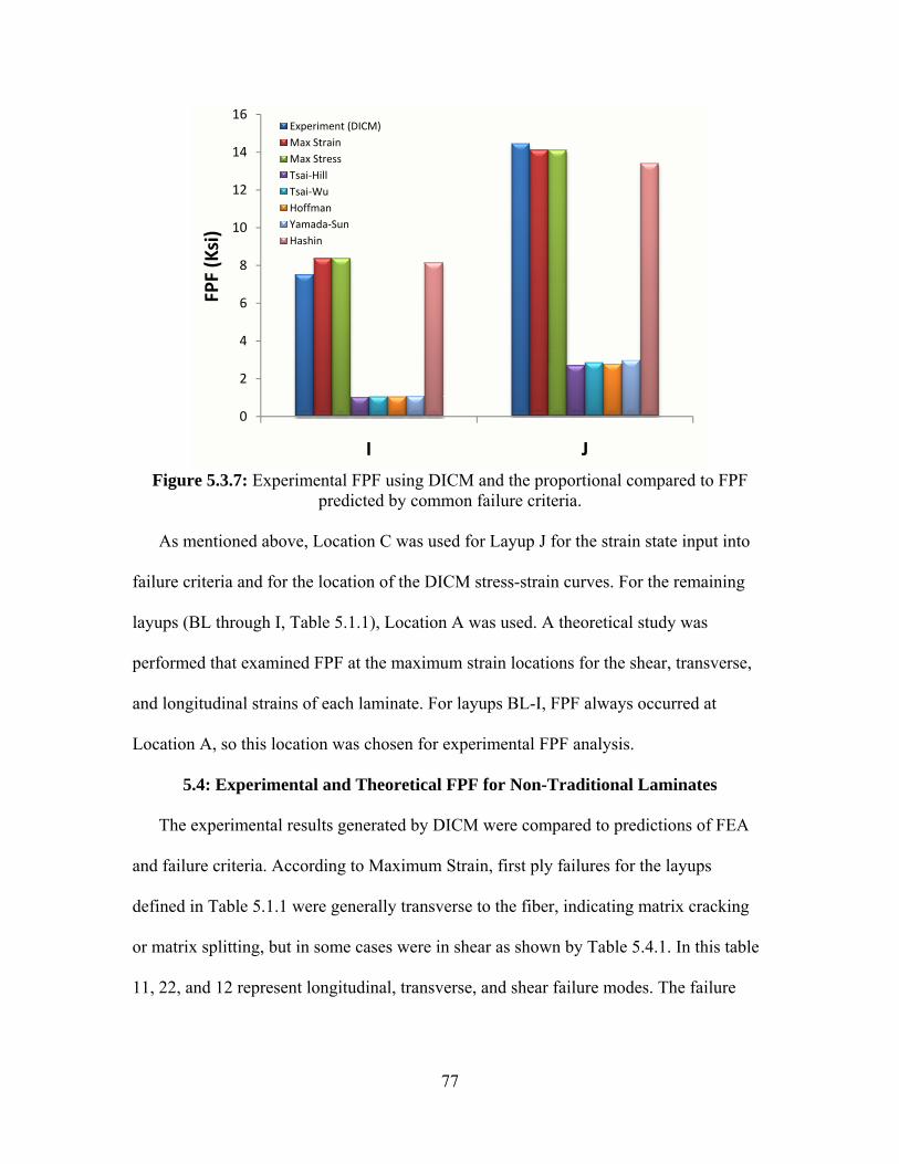
Figure 5.3.7: Experimental FPF using DICM and the proportional compared to FPF
predicted by common failure criteria.
0
2
4
6
8
10
12
14
16
I J
FPF (Ksi)
Experiment (DICM)Max StrainMax StressTsai‐HillTsai‐WuHoffmanYamada‐SunHashin
As mentioned above, Location C was used for Layup J for the strain state input into
failure criteria and for the location of the DICM stress-strain curves. For the remaining
layups (BL through I, Table 5.1.1), Location A was used. A theoretical study was
performed that examined FPF at the maximum strain locations for the shear, transverse,
and longitudinal strains of each laminate. For layups BL-I, FPF always occurred at
Location A, so this location was chosen for experimental FPF analysis.
5.4: Experimental and Theoretical FPF for Non-Traditional Laminates
The experimental results generated by DICM were compared to predictions of FEA
and failure criteria. According to Maximum Strain, first ply failures for the layups
defined in Table 5.1.1 were generally transverse to the fiber, indicating matrix cracking
or matrix splitting, but in some cases were in shear as shown by Table 5.4.1. In this table
11, 22, and 12 represent longitudinal, transverse, and shear failure modes. The failure
77

mode observations made here are theoretical (based on Maximum Strain), compared to
experimentally observed changes in stiffness (equivalent to the “knees” of Fig. 5.1.3).
Table 5.4.1: Failure Modes for FPF as predicted by Maximum Strain Criterion Max Strain BL A B C D E F G H I J
Ply 90º 90º 45º 90º 90º 54º 90º 90º 45º 45º 45º Direction 22 22 12 22 22 12 22 22 12 12 12
Stress-strain behavior for composites is often thought of as being linear until failure.
This is true away from the hole, as would be measured by a strain gage or extensometer.
However, near the hole the stiffness becomes nonlinear (Fig. 5.4.1), indicating the
usefulness of DICM. The polymer behavior of the epoxy matrix could account for some
of this nonlinearity, as polymers can show nonlinearity even in their elastic region.
However, the reloading curve of Figure 5.4.2 shows that damage is in fact occurring. The
“knee” can be seen in the loading and reloading curves of Fig. 5.4.2. This knee indicates
experimental damage initiation, and corresponds to the theoretical FPF as predicted by
maximum strain. It is important to note that the reloading curve of Fig. 5.4.2 does not
follow the final slope of the original loading curve, as would be expected with ideal
damage. This could be due to cracks being sealed upon unloading, or due to nonlinear
effects in the coupon itself. Since the 0º plies of the baseline layup were replaced with 57º
plies to make Layup D, this layup is essentially an in-plane shear coupon, and nonlinear
effects would be expected in Fig. 5.4.2. The Maximum Strain FPF for Fig. 5.4.2 is shown
by a horizontal line indicating the stress, and text indicating the failure ply (90º) and
failure mode (transverse, 22).
78

Figure 5.4.1: Stress vs. longitudinal strain for locations from the hole along Y
(Fig. 2.4.1) for Layup D
0500
100015002000250030003500
0.00 0.01 0.02 0.03 0.04
σ x(p
si)
εxx (in/in)
0.023 in
0.13 in
0.25 in
0.47 in
0
5000
10000
15000
20000
25000
30000
0.00 0.01 0.02 0.03 0.04 0.05
σ x(p
si)
εxx (in/in)
0.039 in
0.039 in (reloading)
Max Strain FPF
90º, 22
Damage initiation
Figure 5.4.2: Stress vs. longitudinal strain for loading and reloading up to 90% UTS, compared to Maximum Strain predicted FPF (Layup D)
Fig. 5.4.3 shows that the proportional limit approximately corresponds to the FPF
predicted by Maximum Strain for Layup F. The proportional limit is more subtle for
some other layups, as only a slight change in stiffness follows FPF. However, FPF can
still be seen clearly as a trend when comparing several coupons of the same layup, as
seen for Layup B in Fig. 5.4.4. Plots similar to Fig. 5.4.4 for all the non-traditional layups
are given in Appendix H. Appendix H is shows the applied stress vs. longitudinal strain
and the applied stress vs. shear strain curves of several coupons for each of the eight non-
79
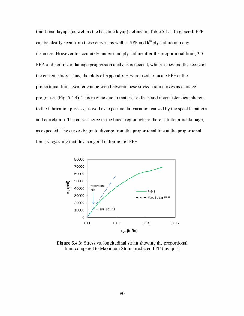
traditional layups (as well as the baseline layup) defined in Table 5.1.1. In general, FPF
can be clearly seen from these curves, as well as SPF and kth ply failure in many
instances. However to accurately understand ply failure after the proportional limit, 3D
FEA and nonlinear damage progression analysis is needed, which is beyond the scope of
the current study. Thus, the plots of Appendix H were used to locate FPF at the
proportional limit. Scatter can be seen between these stress-strain curves as damage
progresses (Fig. 5.4.4). This may be due to material defects and inconsistencies inherent
to the fabrication process, as well as experimental variation caused by the speckle pattern
and correlation. The curves agree in the linear region where there is little or no damage,
as expected. The curves begin to diverge from the proportional line at the proportional
limit, suggesting that this is a good definition of FPF.
0
10000
20000
30000
40000
50000
60000
70000
80000
0.00 0.02 0.04 0.06
σ x(p
si)
εxx (in/in)
F-2-1
Max Strain FPF
FPF: 90º, 22
Proportional limit
Figure 5.4.3: Stress vs. longitudinal strain showing the proportional limit compared to Maximum Strain predicted FPF (layup F)
80

0
10000
20000
30000
40000
50000
60000
70000
80000
90000
0.00 0.01 0.02 0.03 0.04 0.05
σ x(p
si)
εxx (in/in)
0º, 220º, 22
Proportional line
Max Strain FPF
Figure 5.4.4: Stress vs. longitudinal strain for layup B, comparing the proportional limit to Maximum Strain predicted FPF.
Fig. 5.4.5 compares the experimental FPF (from DICM using the proportional limit)
to predictions of FPF from common failure criteria. Table 5.4.2 shows how many
coupons of each layup were tested. This number varies due to the availability of material
for coupon fabrication, as well as DICM difficulty with the speckle pattern in a few of the
coupons tested. The error bars represent one standard deviation. The Maximum Strain
Criterion was best at describing FPF, showing that it was an appropriate choice for
optimization. Similarly, the Maximum Stress Criterion also gave consistently close
approximations to the proportional limit. Hashin Criterion produced values of zero for all
the layups except A, D, and G, where the strain state caused the Hashin Criterion to
reduce to the Maximum Stress Criterion. The remaining quadratic interaction criteria all
poorly predicted FPF. Fig. 5.4.5 and Table 5.4.1 indicate that the Maximum Strain and
Maximum Stress Criteria work well for matrix splitting and shear failure modes. This
81
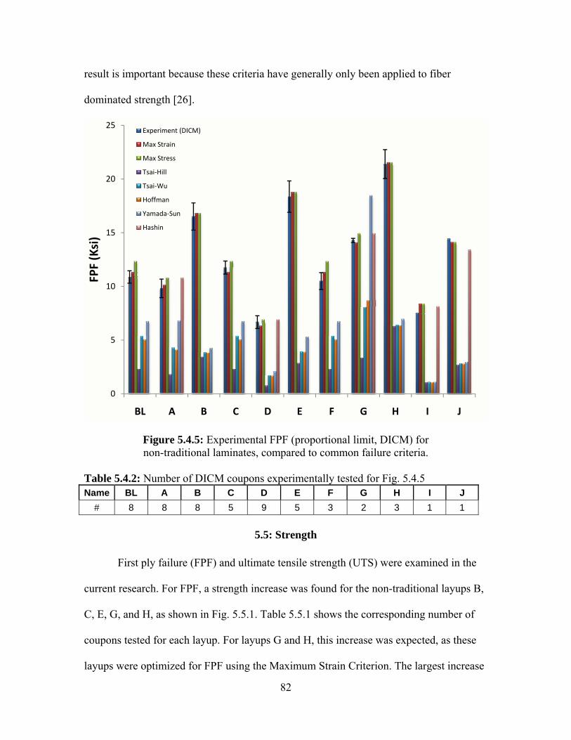
result is important because these criteria have generally only been applied to fiber
dominated strength [26].
0
5
10
15
20
25
BL A B C D E F G H I J
FPF (Ksi)
Experiment (DICM)
Max Strain
Max Stress
Tsai‐Hill
Tsai‐Wu
Hoffman
Yamada‐Sun
Hashin
Figure 5.4.5: Experimental FPF (proportional limit, DICM) for non-traditional laminates, compared to common failure criteria.
Table 5.4.2: Number of DICM coupons experimentally tested for Fig. 5.4.5 Name BL A B C D E F G H I J
# 8 8 8 5 9 5 3 2 3 1 1
5.5: Strength
First ply failure (FPF) and ultimate tensile strength (UTS) were examined in the
current research. For FPF, a strength increase was found for the non-traditional layups B,
C, E, G, and H, as shown in Fig. 5.5.1. Table 5.5.1 shows the corresponding number of
coupons tested for each layup. For layups G and H, this increase was expected, as these
layups were optimized for FPF using the Maximum Strain Criterion. The largest increase
82

in strength was for layup H, which replaced the Baseline 90º plies with 0º plies during
optimization. More surprising were the FPF increases found for layups B, C, and E,
which were kt-optimized. Referring to the FPF failure-modes discussed in Section 5.3
(Table 5.3.1), it is seen that the FPF failure-mode for layups B and E switched from the
Baseline failure ply of 90º in the 22 direction, to a shear failure mode of the ±45º ply (or
±54º for layup E) in the 12 direction. This was also seen for the FPF-optimized layup H,
whose failure ply was ±45º in the 12 direction. In fact, it can be seen that layups B, E, and
H, with the corresponding shear failure modes, have the highest increase in FPF over the
Baseline. This is due to the 90º ply that has been varied to optimize for either kt or FPF.
The 90º ply was replaced with 51º, 54º, and 0º for layups B, E, and H, respectively,
resulting in change of failure mode and the observed increase in FPF. Also notable was
the slight increase in FPF gained by simply varying the order of the Baseline plies, as in
layup C. In this layup, the 0º and 90º ply orders were reversed and thus the 90º ply was
moved further inside the laminate and away from the free edge effects of the surface of
the coupon. A large FPF decrease was found for the kt-optimized layup D, whose 0º plies
were replaced with 57º plies. From Table 2.4.1, layup D had the lowest kt out of the
single angle variations, but also showed the lowest strength, indicating that removing the
primary load bearing plies negatively effects FPF, regardless of the beneficial reduction
of kt. The replacement of the 0º plies with 57º plies essentially made Layup D an in-plane
shear coupon, resulting in the large non-linear behavior exhibited by this laminate. The
kt-optimized Layup A, in which the ±45º plies were replaced with ±54º plies, also
showed an FPF decrease. Thus, by replacing the ±45º plies with plies whose angles are
further away from the load bearing direction, FPF decreased, supporting the conclusions
83

drawn for layup D. This is due to the increase in longitudinal stress resulting from
diverting plies away from the longitudinal axis (0.0181 in/in for BL compared to 0.0202
in/in for A and 0.0324 in/in for D)10, resulting in a lower FPF for the transverse failure
mode of the 90º plies. When the ±45º plies were moved closer to the load bearing axis (as
in the ±21º plies of layup G), or when the number of primary load bearing plies was
increased (90º replaced with 0º plies for layup H), the FPF increased.
0
5
10
15
20
25
BL A B C D E F G H
FPF (Ksi)
Figure 5.5.1: Experimental first ply failure for non-traditional layups using DICM and the proportional limit
Table 5.5.1: Number of DICM coupons experimentally tested for Fig. 5.5.1 Name BL A B C D E F G H
# 8 8 8 5 9 5 3 2 3
10 Calculated at the longitudinal strain maximum (Location A, Fig. 2.4.1) by FEA at 66.7 Ksi.
84
Increases in UTS were found in some of the non-traditional laminates, as shown by
Fig. 5.5.2. The number of coupons tested for each laminate are given in Table 5.5.2.
Selected photographs of coupons at or near failure are shown in Appendix I. The shear
failure of Fig. I.1 and the catastrophic failure of Fig. I.2 are representative of the non-
traditional laminates tested. The largest strength increase was found in layup H (Fig.
5.5.2), whose UTS was above the load capabilities of the MTS tester, and far above the
Baseline. A similar result was obtained for UTS and FPF of Layup H – as the primary
load bearing plies were increased, strength was increased, as expected. The increase in
UTS comes with a material property trade-off, as seen by the reduction of the transverse
modulus of the H layup by over a factor of two (material properties are given in App. A,
Table A.4 and are shown normalized to baseline in Fig. 5.5.3). This reduction in modulus
could be limited during the optimization process using CLT for industrial applications of
this method.
A large increase in UTS was also obtained for layup G, with much less material
property trade off than for layup H (Fig. 5.5.3). For layup G, the ±45º Baseline plies were
replaced with ±21º plies, which resulted in a UTS increase because ply angles were
shifted closer to the primary load bearing axis (the same reason layup G obtained an FPF
increase). Similarly, as plies were shifted away from the longitudinal axis (as for Layup
D and E), the UTS was decreased. Layup D saw the largest decrease in UTS because it
was the only layup without 0º plies.
Strength was increased or decreased depending on the location of the 0º plies. Layup
C switched the order of the Baseline 0º and 90º plies, thus moving the 0º ply outward
resulting in a UTS decrease. Layup F varied the order and moved the 90º ply further
85

inward, resulting in a UTS increase. This result is consistent with those predicted by Tay
et. al. [2], and underscores the importance of stacking sequence.
A UTS increase was also found for layups A and B, which were optimized for kt.
This shows that the strain concentration is an important variable in damage progression
and in designing non-traditional laminates. Specifically, altering the 90º and ±45º plies
can lead to beneficial strength results, while altering the 0º load bearing plies should be
avoided.
0
20
40
60
80
100
120
BL A B C D E F G H
UTS (ksi)
MTS load limit
Figure 5.5.2: Experimental ultimate tensile stress for non-traditional layups Table 5.5.2: Number of DICM coupons experimentally tested for Fig. 5.5.2
Name BL A B C D E F G H # 11 11 11 8 11 6 3 3 3
86

Figure 5.5.3: Material properties of non-traditional laminates normalized to the
baseline (BL) layup
0.00
0.50
1.00
1.50
2.00
2.50
3.00
3.50
BL A B C D E F G H I J
Normalized
Value
ExEyvxyGxy
87

6: Conclusion
Non-traditional laminates provide the opportunity for increased control over strength
and material properties. These laminates can be tailored to meet specific needs and
loading scenarios commonly experienced in engineering structures. This study has shown
the potential for layup tailoring using tools readily available in industry, such as linear
two-dimensional finite element analysis, failure criteria, and classical lamination theory.
These tools can be used to obtain improvements in FPF, as shown by the spatial strain
measurements of DICM and Moiré Interferometry. Furthermore, strength can be
increased, sometimes with little change in material properties.
DICM was found to be a valuable tool for the measurement of full-field surface
strain. DICM was verified using FEA and Moiré Interferometry. The usefulness of this
method lies in the ease in which strain data can be produced; where Moiré Interferometry
can only be used at static loads and requires extensive setup, DICM can be used for the
entire loading of the coupon and only requires a speckle pattern and camera calibration.
Like all measurement techniques, DICM has limits, and is currently not optimal for very
low strains (below 0.001 in/in). However, DICM worked well for strains above 0.001
in/in for T600: 125-33 laminates in open-hole tension. The strain profile and stress-strain
plots revealed the development of the surface strain during damage progression. This was
used to quantify FPF, defined as the proportional limit, which compared well to the
Maximum Strain Criterion. The importance of DICM is underscored by the World-Wide
Failure Exercise [35], in which initial failure data was either not available or of poor
quality. The DICM results presented in Chapter 5 and Appendix G show that the FPF can
be found by locating trends in the stiffness change at the proportional limit.
88
The Maximum Strain and Maximum Stress Failure Criteria performed far better than
any of the other criteria tested for predicting FPF. While the failure mode predictions
remain to be verified by x-ray [42], the results agree with expectations – the majority of
first ply failures were in the transverse direction of the 90º plies due to the large
longitudinal strain at the strain concentration of the hole. This failure mode was predicted
to change to ±45º (or near ±45º) shear failure only for laminates whith the 90º plies
replaced with near 45º plies. The corresponding increase in FPF for these laminates is
also as expected, and was consistent with DICM results.
The FPF load capacity was improved for Layups B, C, E, G, and H, and the UTS load
capacity was improved for Layups A, B, F, G, and H. This improvement was achieved
with little or no variation from the baseline elastic properties for layups A, C, E, and F.
Generally speaking, material properties declined when the ply orientation dominating that
property changed if quasi-isotropic response is desired. For Layup D, the variation in the
0º ply was detrimental to both FPF and UTS due to the large decrease in the longitudinal
modulus, even though the largest strain concentration reduction was achieved for this
layup. Layup H achieved the largest increase in both FPF and UTS, but the replacement
of the 90º ply also caused the largest decrease the transverse modulus. Thus, Layup D and
H are not recommended, and show that the load bearing 0º plies should not be altered,
and that the 90º should not be drastically changed. For other layups, the replacement of a
given ply did not greatly reduce the corresponding material properties. This occurred
during the replacement of the 90º plies with 51º plies for layup B, and the ±45º plies with
±21º plies for layup G. While these replacements resulted in a decrease in the transverse
and shear modulus for Layup B and G, respectively, large increases in strength were
89

found for a relatively small material property trade-off. This suggests that the 90º and
±45º ply orientations could be tailored for a specific loading scenario, with limits placed
on the extent of this variation. If no limits were imposed, Layups B and G are suggested
to increase both FPF and UTS in the open-hole tension loading scenario. Another
significant strength improvement was achieved for Layup C, were the FPF strength
increased simply by switching the order of the 0º and 90º plies. Similarly, for Layup F,
simply moving the 90º ply inward caused an increase in UTS.
This study has shown that non-traditional laminates can be tailored to provide an
increased load capacity for a given loading scenario. The opportunity clearly exists for
strength optimization, though limits should be imposed on the extent of the material
property trade-off. The non-traditional laminates fabricated in this study were optimized
for open-hole tension, and improvements in FPF and UTS were found. The methodology
presented here could be easily adopted in industry using FEA, CLT, and the Maximum
Strain Criteria. Recommendations for further research include CT scans to verify FPF,
nonlinear FEA with damage progression to understand kth ply failures, and analysis of
through-the-thickness effects to account for interlaminar ply interactions.
90

References 1. Soden PD, Kaddour AS, Hinton MJ. Recommendations for designers and researchers
resulting from the world-wide failure exercise. Composites Science and Technology 2004;64:589-604.
2. Composite Materials Handbook, Volume 3: Polymer matrix composites materials usage, design, and analysis. Department of Defense (2002) MIL-HDBK-17-3F.
3. Staab GH. Laminar Composites. © 1999 Butterworth-Heinemann. 4. Wang J, Callus PJ, Bannister MK. Experimental and numerical investigation of the
tension and compression strength of un-notched and notched quasi-isotropic laminates. Composite Structures 2003;64:297-306.
5. Tay TE, Liu G, Tan VBC. Damage Progression in Open-hole Tension Laminates by the SIFT-EFM Approach. Journal of Composite Materials 2005;0:1-22.
6. Park H-J. Bearing failure analysis of mechanically fastened joints in composite laminates. Journal of Composite Structures 2001;53:199-211.
7. Park H-J. Bearing failure analysis of mechanically fastened joints in composite laminates. Journal of Composite Structures 2001;53:199-211.
8. Oh JH, Kim YG, Lee DG. Optimum bolted joints for hybrid composite materials. Journal of Composite Structures 1997;38(1-4):329-341.
9. Todoroki A, Sasada N, Miki M. Object-Oriented Approach to Optimize Composite Laminated Plate Stiffness with Discrete Ply Angles. Journal of Composite Materials 1996;30(9):1020-1041.
10. Starikov, Roman, Schon, Joakim. Quasi-static behavior of composite joints with protruding-head bolts. Jour. Composite Structures 2005;51:411-425.
11. Yan UM, Sun HT, Wei WD, Chang FK. Response and Failure of Composite Plates with a Bolt-Filled Hole. Technical Report (1998) DOT/FAA/AR-97/85.
12. Kostreva K, Zhao Y, Thomas F. Through-The-Thickness Compression (TTTC) Properties For Laminated Composites – An Experimental Study. AIAA 2003-1508 971-978.
13. Dano M-L, Gendron G, Picard A. Stress and failure analysis of mechanically fastened joints in composite laminates. Composite Structures 2000;50:287-296.
14. McCarthy MA, McCarthy CT, Lawlor VP, Stanley WF. Three-dimensional finite element analysis of single-bolt, single-lap composite bolted joints: part I-model development and validation. Composite Structures 2005;71:140-158.
15. McCarthy CT, McCarthy MA, Lawlor VP. Progressive damage analysis of multi-bolt composite joints with variable bolt-hole clearances. Composites, Part B: engineering, 2005;36:290-305.
16. Sun H-T, Chang F-K, Qing X. The Response of Composite Joints with Bolt-Clamping Loads, Part I: Model Development, Journal of Composite Materials, 1999;36(1):47-67.
17. Sun H-T, Chang F-K, Qing X. The Response of Composite Joints with Bolt-Clamping Loads, Part II: Model Verification. Journal of Composite Materials 1999;36(1):69-92.
18. Tan SC. Design of Composite Laminate Containing an Opening. 30th National SAMPE Symposium, March 19-21 (1985) 1168-1178.
91

19. Tsau L-R, Chang Y-H, Tsao F-L. The Design of Optimal Stacking Sequence for Laminated FRP Plates with Inplane Loading. Computers and Structures 1995;55(4):565-580.
20. Barakat SA, Abu-Farsakh GA. The use of an energy-based criterion to determine optimum configurations of fibrous composites. Composites Science and Technology 1999;59:1891-1899.
21. Shi CH. Approximate Interlaminar Stresses Local to a Circular Hole in a Symmetric Angle-Ply Laminate Under In-plane Shear. Theoretical and Applied Fracture Mechanics 1990;14:57-53.
22. Treasurer PJ. Characterization and analysis of damage progression in non-traditional composite laminates with circular holes. Georgia Institute of Technology Thesis 2006.
23. Muc A. Optimal fibre orientation for simply-supported, angle-ply plates under biaxial compression. Composite Structures 1998;9:161-172.
24. Gosse JH. A Damage Functional Methodology for Assessing Post-Damage Initiation Environments in Composite Structure. AIAA 2004-1788 3039-3043.
25. Tay TE, Tan VBC, Tan SHN. Element-Failure: An Alternative to Material Property Degradation Method for Progressive Damage in Composite Structures. Journal of Composite Materials 2005;39(18):1659-1675.
26. Gibson RF. Principles of Composite Material Mechanics, 2nd Edition. © 2007 Taylor & Francis Group, LLC.
27. Hashin Z. Failure Criteria for Unidirectional Fiber Composites. Journal of Applied Mechanics 1980;47:329-334.
28. Hill R. A theory of the yielding of plastic flow of anisotropic metals. Proceedings of the Royal Society of London. Series A, Mathematical and Physical Sciences 1948;193(1033):281-297.
29. Tsai SW. Strength theories of filamentary structures. In Schwartz, R.T. and Schwartz, H.S. eds., Fundamental Aspects of Fiber Reinforced Plastic Composites, chapter 1 (1968) 3-11. Wiley Interscience, New York.
30. Tsai SW, Wu EM. A general theory of strength for anisotropic materials. Journal of Composite Materials, 1971;5:58-80.
31. Hoffman O. The Brittle Strength of Orthotropic Materials. Journal of Composite Materials 1971;5:58.
32. Sizaire R. FesResPost User Manual, Version 2.9.4. 05/20/2007 [email protected]. 33. Tsai SW, Hahn, HT. Introduction to Composite Materials. Technomic Publishing Co.,
Lancaster, PA, 1980. 34. Kam TY, Sher HF. Nonlinear and First-Ply Failure Analyses of Laminated
Composite Cross-Ply Plates. Journal of Composite Materials 1995;29(4):463-482. 35. Zinoviev PA, Grigoriev SV, Labedeva OV, Tairova LR. Strength of multilayered
composites under plane stress state. Composite Science and Technology 1998;58:1209-1224.
36. Bogetti TA, Hoppel CPR, Harik VM, Newill JF, Burns BP. Predicting the nonlinear response and progressive failure of composite laminates. Composite Science and Technology 2004;64(3-4):329-342.
92
37. Puck A., Shurmann H. Failure analysis of FRP laminates by means of physically based phenomenological models. Composite Science and Technology 1998;58:1179-1208.
38. Puck A., Shurmann H. Failure analysis of FRP laminates by means of physically based phenomenological models. Composite Science and Technology 1998;58:1179-1208.
39. Liu K-S, Tsai SW. Progressive quadratic failure criterion of a laminate. Composite Science and Technology 1998;58:1023-1032.
40. Mallick PK. Composites Engineering Handbook. © 1197 Marcel Dekker, Inc. 41. Ugural AC. Mechanical Design, An Integrated Approach. McGraw-Hill © 2004, pp.
777. 42. Kothidar A. Use of finite element method to evaluate the strength response of notched
composite laminates under tension. Washington State University Thesis, to be published July 2008.
43. Schreier HW, McNeill SR, Sutton MA. Digital Image Correlation: Principles, Developments and Hands-on Experiments for 2D and 3D Computer Vision Systems. (2006) Correlated Solutions, Incorporated.
44. Helm J, Kurts S. Digital image correlation-based experimental stress analysis of reinforced concrete beams, strengthened using carbon composites. SPIE-IS&T 2005;5665:40-50.
45. Whitney JM, Nuismer RJ. Stress fracture criteria for laminated composites containing stress concentrations. Journal of Composite Materials 1974;8:253-65.
46. Ambu R, Aymerich F, Bertolino F. Investigation of the effect of damage on the strength of notched composite laminates by digital image correlation. Journal of Strain Analysis 2005;40(5):451-461.
47. Cheng P, Sutton MA, Schreier HW, McNeill S.R. Full-field Speckle Pattern Image Correlation with B-Spline Deformation Function. Experimental Mechanics 2002;42(3):334-352.
48. Post D, Han B, Ifju P. High Sensitivity Moiré. Springer-Verlag 1994. 49. Liu H, Cartwright A.N., Basaran C, Casey W. Moiré Interferometry for
Microelectronics Packaging Interface Fatigue Reliability. GaAsMANTECH Conference 2002.
50. Post D, Czarnek R, Joh D, Wood J. Deformation measurement of composite multi-span beam shear specimens by Moiré Interferometry. NASA Contracter Report 1984; 3844.
51. Nicola SD, Ferraro P. Fourier transform method of fringe analysis for Moiré Interferometry. J. Opt. A: Pure Appl. Opt. 2000;2:228-233.
52. Stelmkas JW, Zink AG, Loferski JR. Image correlation analysis of multiple-bolt wood connections. Wood and Fiber Science 1997;29(3):210-227.
53. Halpin, JC. Primer on Composite Materials: Analysis. 1984 Technnomic Publishing Co., Lancaster, PA.
54. Whitney JM, Nuismer RJ. Stress fracture criteria for laminated composites containing stress concentrations. Journal of Composite Materials 1974;8:253-65.
55. Rasouli S, Tavassolly MT. Moiré technique improves the measurement of atmospheric turbulence parameters. © 2008 SPIE DOI: 10.1117/2.1200702.0569
93

56. Rasouli S, Tavassolly MT. Moiré technique improves the measurement of atmospheric turbulence parameters. © 2008 SPIE DOI: 10.1117/2.1200702.0569
57. PenWell. Moiré Experimental Setup. images.pennnet.com Copyright © 2008: PennWell Corporation, Tulsa, OK; All Rights Reserved
58. Callister, W.D. Materials Science and Engineering, An Introduction. Seventh Edition. John Wiley & Sons, Inc. © 2007 pp. 137, A8
94

Appendix A: Tables
Table A.1: T600: 125-33 Composite Material System (psi) 11 E1 = 19.73x10⁶ ± 0.65x10⁶ E2 = 1.38x10⁶ ± 0.021x10⁶ E3 = E2 G12 = 0.81x10⁶ ± 0.022x10⁶ G13 = G12 ν12 = 0.298 ± 0.019 ν23 = 0.35 ν13 = ν12 sL
(+) = 332.8x10³ ± 16.2x10³
sT(+) = 6.28x10³ ± 0.63x10³ sLT = 9.03x10³ ± 0.37x10³ sL
(-) = 209x103
sT(-) = 33x103
Table A.2: Aluminum Alloy 707512 (psi) Ex = 10.3x10⁶ ν = 0.33 Table A.3: Fabricated laminates
Designation Layup Description Method BL [(45/90/-45/0)2]s baseline Baseline A [(54/90/-54/0)2]s vary 45 kt B [(45/51/-45/0)2]s vary 90 kt C [(45/0/-45/90)2]s vary order 1 kt D [(45/90/-45/57)2]s vary 0 kt E [(54/54/-54/0)2]s vary 45&90 kt F [(45/-45/90/0)2]s vary order 2 literature G [(21/90/-21/0)2]s vary 45 FPF H [(45/0/-45/0)2]s vary 90 FPF I [(±45)4]s shear failure failure mode J [0]16 uniaxial faiure failure mode
Table A.4: Material properties using classical lamination theory
Property BL A B C D E F G H I J Ex (Msi) 7.7 6.7 7.0 7.7 3.2 6.4 7.7 12.8 11.4 2.8 19.7 Ey (Msi) 8 9 4 8 8 6 8 6 3 3 1
vxy 0.23 0.23 0.23 0.23 0.23 0.23 0.23 0.22 0.67 0.75 0.30 Gxy (Msi) 3 3 4 3 4 4 3 2 3 5 1
Table A.5: Failure indexes of non-traditional laminates at Location A
Max Strain BL A B C D E F G H I J e1/e1c 0.48 0.41 1.62 0.48 0.91 0.10 0.48 0.27 1.25 0.47 1.23 e2/e2c 5.89 6.59 3.83 5.89 10.58 3.22 5.89 4.74 3.05 1.27 0.20
e12/e12c 0.00 0.00 0.00 0.00 0.00 2.44 0.00 0.00 0.00 5.58 0.00
11 Properties were found from in-plane tests of [0]6, [90]16, and [±45]2s that were performed at the WSU Environmental Exposure Facility by Matt Shultz. The out-of-plane material properties (ν23) and compressive strengths were estimated from AS4/3501-6 [40] where the standard deviation was not reported. 12 Material properties for Aluminum Alloy 7075 from [57].
95

Appendix B: Coupon Dimensions
96

Appendix C: Convergence Study for Locations (X,Y)
Top of hole (0, 0.125)
0.014
0.0142
0.0144
0.0146
0.0148
0.015
0.0152
0.0154
0.0156
0.0158
0 500 1000 1500 2000 2500 3000 3500 4000 4500
Elements
Axi
al S
trai
nTop of hole (0, 0.125)
-0.005000
-0.004500
-0.004000
-0.003500
-0.003000
-0.002500
-0.002000
-0.001500
-0.001000
-0.000500
0.0000000 500 1000 1500 2000 2500 3000 3500 4000 4500
Elements
Tran
sver
se S
trai
n
Side of hole (0.125, 0)
0.00E+00
2.00E-04
4.00E-04
6.00E-04
8.00E-04
1.00E-03
1.20E-03
1.40E-03
1.60E-03
1.80E-03
0 500 1000 1500 2000 2500 3000 3500 4000 4500
Elements
Axi
al S
trai
n
Side of hole (0.125, 0)
-0.006000
-0.005000
-0.004000
-0.003000
-0.002000
-0.001000
0.0000000 500 1000 1500 2000 2500 3000 3500 4000 4500
Elements
Tran
sver
se S
trai
n
Top edge (0, 0.75)
-0.001466
-0.001465
-0.001465
-0.001464
-0.001464
-0.001463
-0.001463
-0.001462
-0.0014620 500 1000 1500 2000 2500 3000 3500 4000 4500
Elements
Tran
sver
se S
trai
n
Top edge (0, 0.75)
0.004832
0.004834
0.004836
0.004838
0.00484
0.004842
0.004844
0.004846
0.004848
0.00485
0 500 1000 1500 2000 2500 3000 3500 4000 4500
Elements
Axi
al S
trai
n
Side edge (6, 0)
0
0.001
0.002
0.003
0.004
0.005
0.006
0 500 1000 1500 2000 2500 3000 3500 4000 4500
Elements
Axi
al S
trai
n
Side edge (6, 0)
-0.001800
-0.001600
-0.001400
-0.001200
-0.001000
-0.000800
-0.000600
-0.000400
-0.000200
0.0000000 500 1000 1500 2000 2500 3000 3500 4000 4500
Elements
Tran
sver
se S
trai
n
97

Appendix D: Optimization using FEA
D.1: Decrease the strain concentration, kt
Vary ±45º
2.45
2.50
2.55
2.60
2.65
2.70
2.75
2.80
2.85
35 40 45 50 55 60 65 70
θ
kt354045505253545556576065
Vary 90º
2.35
2.40
2.45
2.50
2.55
2.60
40 50 60 70 80 90 100
θ
kt
90857565535251504940
Vary 0º
1.80
1.90
2.00
2.10
2.20
2.30
2.40
2.50
2.60
2.70
0 10 20 30 40 50 60 70
θ
kt
0510152025303545505254555657586065
98

D.2: Increase the first ply failure, FPF
Vary ±45º
0
200
400
600
800
1000
1200
1400
1600
1800
0 10 20 30 40 50 60 70
θ
FPF
(lbs)
Max stressMax strainTsai-WuTsai-Hill
24º
Vary 90º
0
500
1000
1500
2000
2500
3000
3500
0 10 20 30 40 50 60 70 80 90 100
θ
FPF
(lbs) Max stress
Max strainTsai-HillTsai-Wu
Vary 0º
0
200
400
600
800
1000
1200
1400
0 5 10 15 20 25 30
θ
FPF
(lbs) Max stress
Max strainTsai-HillTsai-Wu
99

D.3: Example of a double angle optimization
100

Appendix E: Matlab Program for Failure Criteria
%Daniel Stone %This program uses failure theories to predict strength of a composite %Inputs are the 2D strain state at a point (FEA), load, and ply angles %Outputs are the strengths for each ply from max stress, max strain, %Tsai‐Hill, Tsai‐Wu, Hoffman, Hashin, and Yamada‐Sun clear clc format long %Material properties for T600: 125‐33 E1=19.73*10^6; E2=1.3775*10^6; G12=0.80*10^6; v12=0.2976; v21=0.02575; %Stiffness matrix Q11=E1/(1‐v12*v21); Q12=v12*E2/(1‐v12*v21); Q22=E2/(1‐v12*v21); Q66=G12; Q=[Q11 Q12 0, Q12 Q22 0, 0 0 Q66]; %Strength %Ultimate tensile stress S1=332.8*10^3; S2=6.28*10^3; S12=9.031*10^3; %Ultimate compressive stress S1c=209*10^3; S2c=33*10^3; %Ultimate tensile strain e1=S1/E1; e2=S2/E2; e12=S12/G12; %Ultimate compressive strain e1c=S1c/E1; e2c=S2c/E2; %Input ply angles theta(1)=abs(input('1rst ply angle?')); theta(2)=abs(input('2nd ply angle?')); theta(3)=abs(input('3rd ply angle?')); theta(4)=abs(input('4rth ply angle?')); %Input load and strain state load=input('Load (lbs)?'); epsilonx=input('Axial Strain?'); epsilony=input('Transverse Strain?'); gammaxy=input('Shear Strain?'); %Strain vector at a location on the laminate e=[epsilonx epsilony gammaxy/2]';
101

%Ply angle vector theta=theta'; %Ply angle vector in radians theta=theta*pi/180; %Calculate strains and stresses in the fiber direction for k=1:3 ply=theta(k); c=cos(ply); s=sin(ply); %Transformation matrix T=[c^2 s^2 2*c*s, s^2 c^2 ‐2*c*s, ‐c*s c*s (c^2‐s^2)]; %Strain vector in the fiber direction strain_fiber=T*e; epsilon11(k)=strain_fiber(1); epsilon22(k)=strain_fiber(2); gamma12(k)=2*strain_fiber(3); %Stress vector in the fiber direction stress_fiber=Q*[epsilon11(k) epsilon22(k) gamma12(k)]'; sigma11(k)=stress_fiber(1); sigma22(k)=stress_fiber(2); tau12(k)=stress_fiber(3); end %Maximum stress criterion for k=1:3 %failure index if sigma11(k)>0 maxstress(1)=abs(sigma11(k)/S1); else maxstress(1)=abs(sigma11(k)/S1c); end if sigma22(k)>0 maxstress(2)=abs(sigma22(k)/S2); else maxstress(2)=abs(sigma22(k)/S2c); end maxstress(3)=abs(tau12(k)/S12); fi_maxstress = max(maxstress); %strength of ply failure_maxstress(k)=load/fi_maxstress; end %ply failures failure_maxstress; %Maximum strain criterion for k=1:3 %failure index if epsilon11(k)>0 maxstrain(1)=abs(epsilon11(k)/e1); else maxstrain(1)=abs(epsilon11(k)/e1c); end if epsilon22(k)>0
102
maxstrain(2)=abs(epsilon22(k)/e2); else maxstrain(2)=abs(epsilon22(k)/e2c); end maxstrain(3)=abs(gamma12(k))/e12; %To see failure indices, delete percentages in the following lines: %k %maxstrain fi_maxstrain=max(maxstrain); %strength of ply failure_maxstrain(k)=load/fi_maxstrain; end %kth ply failure failure_maxstrain; %Tsai‐Hill criterion for k=1:3 %failure index fi_tsaihill = (sigma11(k)/S1)^2 + (sigma22(k)/S2)^2 + (tau12(k)/S12)^2 ‐ sigma11(k)*sigma22(k)/S1^2; %strength of ply failure_tsaihill(k)=load/fi_tsaihill; end %kth ply failure failure_tsaihill; %Tsai‐Wu criterion for k=1:3 %failure index fi_tsaiwu = sigma11(k)^2/(S1*S1c) + sigma22(k)^2/(S2*S2c) + (tau12(k)/S12)^2 + (1/S1‐1/S1c)*sigma11(k) + (1/S2‐1/S2c)*sigma22(k) ‐ sigma11(k)*sigma22(k)/(S1*S1c*S2*S2c)^.5; %strength of ply failure_tsaiwu(k)=load/fi_tsaiwu; end %kth ply failure failure_tsaiwu; %Hoffman criterion (same as Tsai‐Wu except last term) for k=1:3 %failure index fi_hoffman = sigma11(k)^2/(S1*S1c) + sigma22(k)^2/(S2*S2c) + (tau12(k)/S12)^2 + (1/S1‐1/S1c)*sigma11(k) + (1/S2‐1/S2c)*sigma22(k) ‐ sigma11(k)*sigma22(k)/(2*S1*S1c); %strength of ply failure_hoffman(k)=load/fi_hoffman; end %kth ply failure failure_hoffman; %Hashin criterion for k=1:3 %reserve factors if sigma11(k) > 0 fi_1 = ((sigma11(k)/S1)^2 + (tau12(k)/S12)^2)^.5; else fi_1 = abs(sigma11(k))/S1c; end if sigma22(k) > 0 fi_2 = ((sigma22(k)/S2)^2 + (tau12(k)/S12)^2)^.5;
103
else a = (sigma22(k)/2*S12)^2 + (tau12(k)/S12)^2; b = ((S2c/2*S12)^2‐1)*abs(sigma22(k)/S2c); c = ‐1; fi_2 = (2*a)/(‐b+(b^2‐4*a*c)^.5); end %failure index fi_hashin = max(fi_1,fi_2); %strength of ply failure_hashin(k)=load/fi_hashin; end %kth ply failure failure_hashin; %Yamada‐sun criterion for k=1:3 %failure index if sigma11(k)>0 fi_yamadasun=(sigma11(k)/S1)^2 + (tau12(k)/S12)^2; else fi_yamadasun=(sigma11(k)/S1c)^2 + (tau12(k)/S12)^2; end %strength of ply failure_yamadasun(k)=load/fi_yamadasun; end %kth ply failure failure_yamadasun; %first ply failure FPF_maxstress=min(failure_maxstress) FPF_maxstrain=min(failure_maxstrain) FPF_tsaihill=min(failure_tsaihill) FPF_tsaiwu=min(failure_tsaiwu) FPF_hoffman=min(failure_hoffman) FPF_hashin=min(failure_hashin) FPF_yamadasun=min(failure_yamadasun)
104

Appendix F: Selected Strain Contours
Figure F.1: Longitudinal strain contours for layup D at 9.43 Ksi
Figure F.2: Longitudinal strain contours for layup I at 14.9 Ksi
105

Figure F.3: Longitudinal strain contours for layup G at 18.3 Ksi
Figure F.4: Transverse strain contours for layup A at 39.3 Ksi
106
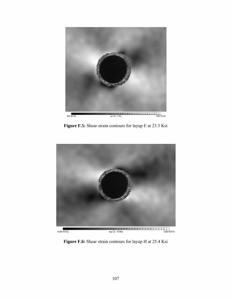
Figure F.5: Shear strain contours for layup E at 23.3 Ksi
Figure F.6: Shear strain contours for layup H at 25.4 Ksi
107

Appendix G: DICM/Moiré Interferometry Strain Contour Comparison
Figure G.1: Longitudinal Moiré deformation/DICM strain contours for the baseline layup at an applied stress of 19 Ksi
Figure G.2: Transverse Moiré deformation/DICM strain contours for the baseline layup at an applied stress of 19 Ksi
108
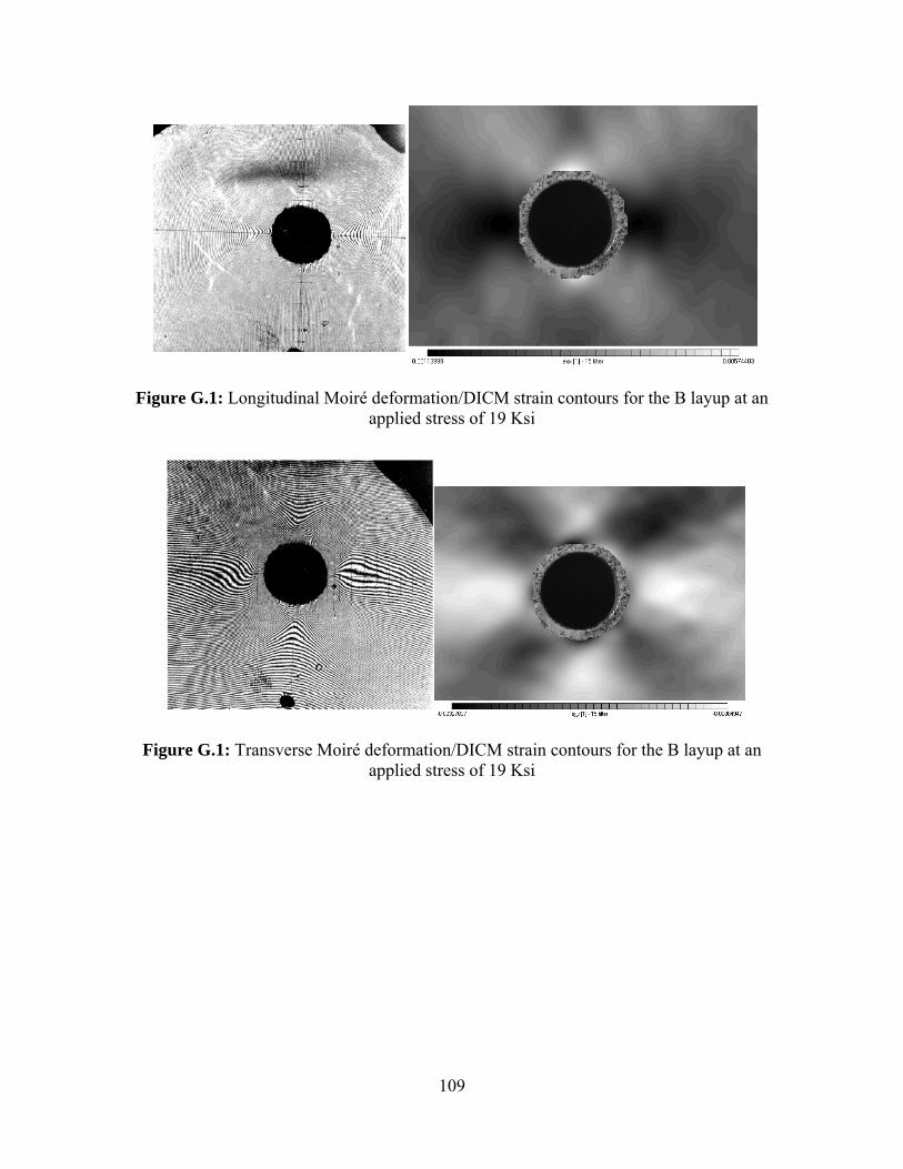
Figure G.1: Longitudinal Moiré deformation/DICM strain contours for the B layup at an applied stress of 19 Ksi
Figure G.1: Transverse Moiré deformation/DICM strain contours for the B layup at an applied stress of 19 Ksi
109
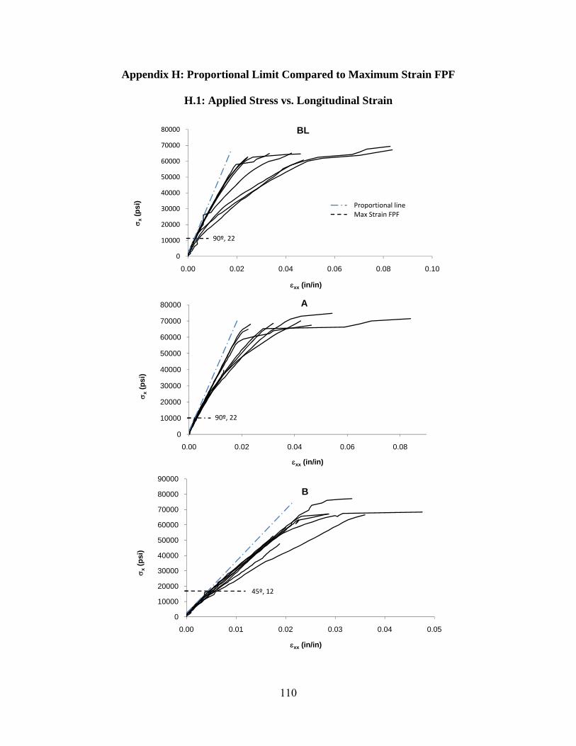
Appendix H: Proportional Limit Compared to Maximum Strain FPF
H.1: Applied Stress vs. Longitudinal Strain
0
10000
20000
30000
40000
50000
60000
70000
80000
0.00 0.02 0.04 0.06 0.08 0.10
σ x(p
si)
εxx (in/in)
BL
90º, 22
Proportional lineMax Strain FPF
0
10000
20000
30000
40000
50000
60000
70000
80000
0.00 0.02 0.04 0.06 0.08
σ x(p
si)
εxx (in/in)
A
90º, 22
0
10000
20000
30000
40000
50000
60000
70000
80000
90000
0.00 0.01 0.02 0.03 0.04 0.05
σ x(p
si)
εxx (in/in)
B
45º, 12
110
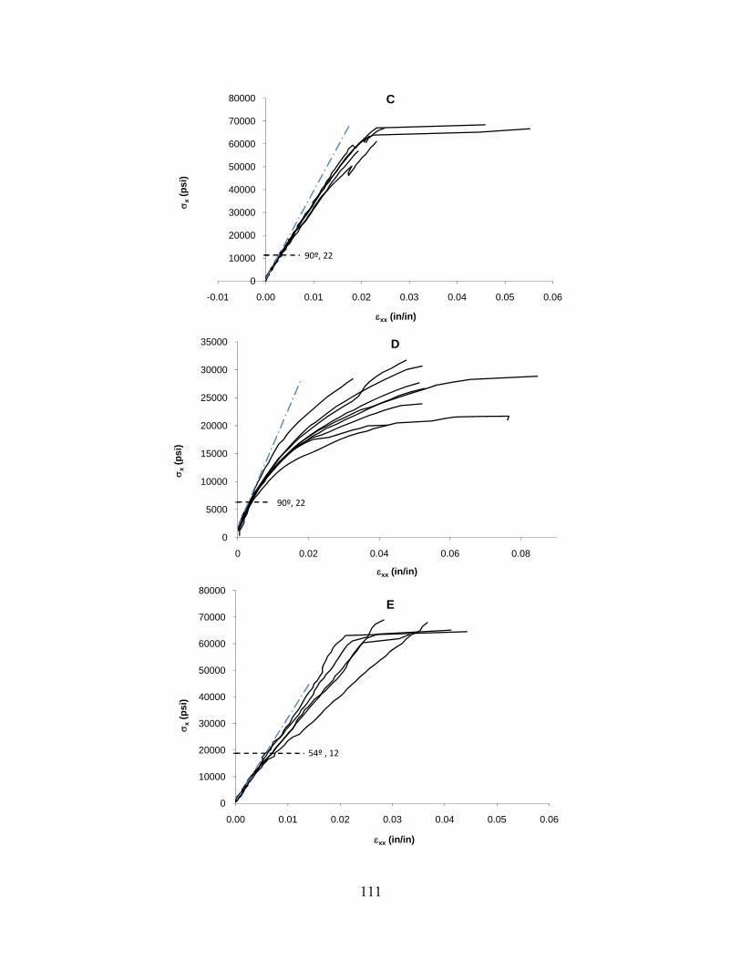
0
10000
20000
30000
40000
50000
60000
70000
80000
-0.01 0.00 0.01 0.02 0.03 0.04 0.05 0.06
σ x(p
si)
εxx (in/in)
C
90º, 22
0
5000
10000
15000
20000
25000
30000
35000
0 0.02 0.04 0.06 0.08
σ x(p
si)
εxx (in/in)
D
90º, 22
0
10000
20000
30000
40000
50000
60000
70000
80000
0.00 0.01 0.02 0.03 0.04 0.05 0.06
σ x(p
si)
εxx (in/in)
E
54º , 12
111

0
10000
20000
30000
40000
50000
60000
70000
80000
0.00 0.01 0.02 0.03 0.04 0.05 0.06
σ x(p
si)
εxx (in/in)
F
90º, 22
0
20000
40000
60000
80000
100000
120000
0.00 0.01 0.02 0.03 0.04
σ x(p
si)
εxx (in/in)
G
90º, 22
0
20000
40000
60000
80000
100000
120000
0.000 0.005 0.010 0.015 0.020
σ x(p
si)
εxx (in/in)
H
45º, 12
112

H.2: Applied Stress vs. Shear Strain
0
10000
20000
30000
40000
50000
60000
70000
80000
-0.01 0.00 0.01 0.02 0.03 0.04 0.05
σ x(p
si)
εxy (in/in)
BL
90º, 22
0
10000
20000
30000
40000
50000
60000
70000
80000
-0.005 0.000 0.005 0.010 0.015 0.020 0.025 0.030 0.035 0.040
σ x(p
si)
εxy (in/in)
A
90º, 22
0
10000
20000
30000
40000
50000
60000
70000
80000
90000
-0.005 0.000 0.005 0.010 0.015 0.020
σ x(p
si)
εxy (in/in)
B
45º, 12
113
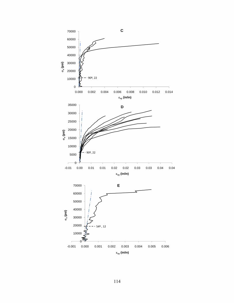
0
10000
20000
30000
40000
50000
60000
70000
0.000 0.002 0.004 0.006 0.008 0.010 0.012 0.014
σ x(p
si)
εxy (in/in)
C
90º, 22
0
5000
10000
15000
20000
25000
30000
35000
-0.01 0.00 0.01 0.01 0.02 0.02 0.03 0.03 0.04 0.04
σ x(p
si)
εxy (in/in)
D
90º, 22
0
10000
20000
30000
40000
50000
60000
70000
-0.001 0.000 0.001 0.002 0.003 0.004 0.005 0.006
σ x(p
si)
εxy (in/in)
E
54º , 12
114

0
10000
20000
30000
40000
50000
60000
70000
80000
-0.005 0.000 0.005 0.010 0.015 0.020 0.025 0.030 0.035
σ x(in
/in)
εxy (in/in)
F
90º, 22
0
20000
40000
60000
80000
100000
120000
0.000 0.003 0.005 0.008 0.010 0.013 0.015 0.018 0.020
σ x(in
/in)
εxy (in/in)
G
90º, 22
115

Appendix I: Selected Laminates at or Near Failure
Figure I.1: Layup A at Failure
Figure I.2: Layup B at Failure
116

Figure I.3: Layup BL at 97% UTS
Figure I.3: Layup G at failure
117