the influence of anisotropy on the consolidation …...(esp). for over–consolidated isotropic...
TRANSCRIPT

The influence of anisotropy on the
consolidation behaviour of peat
C. Zwanenburg
October 2005

ii

The influence of anisotropy on the
consolidation behaviour of peat
PROEFSCHRIFT
ter verkrijging van de graad van doctoraan de Technische Universiteit Delft,
op gezag van de Rector Magnificus Prof. dr. ir. J.T. Fokkema,voorzitter van College voor Promoties,
in het openbaar te verdedigenop woensdag 7 december 2005 om 10:30 uur
door Cornelis ZWANENBURGciviel ingenieur
geboren te Rotterdam
Dit proefschrift is goedgekeurd door de promotor:Prof. dr. ir. F.B.J. Barends
Samenstelling promotiecommissie:
Rector Magnificus, voorzitterProf. dr. ir. F.B.J. Barends, Technische Universiteit Delft, promotorProf. dr. J.P. Magnan, Laboratoire des Ponts et ChausseesProf. dr. ir. F. Molenkamp, Technische Universiteit DelftProf. dr. ir. A. Verruijt, Technische Universiteit DelftProf. ir. A.F. van Tol, Technische Universiteit DelftProf. drs. ir. H. Vrijling, Technische Universiteit Delftdr. ir. E.J. den Haan, GeoDelft
Published and distributed by: DUP Science
DUP Science is an imprint ofDelft University PressP.O.Box 982600 MG DelftThe NetherlandsTelephone: +31 15 27 85 678Telefax: +31 15 27 85 706E–mail [email protected]
ISBN 90-407-2615-9
Keywords: geotechnics, consolidation, anisotropy, peat
Copyright c©2005 by C. Zwanenburg
All rights reserved. No part of the material protected by this copyright notice may be reproducedor utilised in any form or by any means, electronic or mechanical, including photocopying,recording or by any information storage and retrieval system, without written permission fromthe publisher: Delft University Press.
Printed in The Netherlands

Acknowledgement
This study is conducted at Delft University of Technology and financially supported by the DIOCproject and GeoDelft. During the four and a half years it took me to complete this study I wassupported by a large number of people. With this opportunity I would like thank them.
First of all I would I like to thank my promotor Prof. Frans Barends who gave me the oppor-tunity to enrich my practical experience I was building up as a consultant by a fundamental studyat Delft University of Technology. Over the years he taught me how powerful mathematics can bein describing nature in general and soft soil behaviour in particular.
Next I would like to thank the geotechnical engineering group at Delft University of Technol-ogy who offered me a quiet place to work, while always willing to help. Especially I would like tomention Han de Visser who helped me to solve all kinds of practical problems in retrieving soilsamples and conducting laboratory tests. For example without his help I would not have possessedthe perfect membranes needed triaxial testing.
I would like to express gratitude to GeoDelft, especially Gerben Beetstra who enabled mysecondment at Delft University of Technology and Jan de Feijter who allowed me to work in thelaboratory. I would like thank: Aad Schapers and Aad van Slingerland who taught me the basicsof working in a geotechnical laboratory, Lambert Smidt who was always willing to help with thesoftware controlling the test facilities and Willem van Pernis and Ruud van der Berg who helpedme in conducting large scale experiments.
I’m especially grateful to Evert den Haan who followed my study critically and, in discussingthe results, especially the laboratory measurements, gave me a better understanding in soft soilbehaviour and helped me to focus.
Finally but most important I would like to thank Diane who hasn’t seen much of me in the lastyears but was always encouraging me to continue. I hope that I will ever be able to make that upto her.
v

vi ACKNOWLEDGEMENT
Abstract
The influence of anisotropy on the consolidation behaviour of peat
Soft soil is often described as an anisotropic heterogeneous material. Standard soil investigationmainly involves vertically retrieved samples. Information on the parameters working in the horizon-tal direction remains scarce. Principally each soil property like permeability, stiffness or strengthmight show anisotropic behaviour. This thesis focuses on anisotropy in stiffness and the possibilityto use conventional laboratory measurement techniques to determine the level of anisotropy instiffness.
One type of soft soil that particularly is expected to behave anisotropically is peat. A possibleanisotropy in stiffness of peat can be explained by the presence of fibres. Depending on the rateof humification and organic origin the fibres contribute to the stiffness of peat. If the peat fibresare mainly aligned in one plane it is to be expected that the stiffness perpendicular to this planedeviates from the stiffness working in this plane. Anisotropy due to the presence of fibres is knownas structural anisotropy. Since peat is a soft and very compressible material asymmetrical loadingmight also induce anisotropy in stiffness. This type of anisotropy is known as induced anisotropy.
Consolidation behaviour of soil is strongly influenced by the stiffness of the considered material.For special conditions the pore pressure development during consolidation differs from the usuallyfound monotonic decrease. These special conditions are e.g. found when a conventional triaxialsample with a stiff plate on top and bottom is allowed to drain at the outer radius. Then theouter radius of the sample tends to drain at an early stage of the consolidation process while inthe inner core of the sample dissipation of pore water takes place at a later stage. Consolidationof the outer radius of the sample leads to volumetric strain in this area. This volumetric strain incombination with the stiff plate on top leads to a redistribution of stresses in which a part of theload carried by the outer radius is transferred to the yet unconsolidated inner core of the sample.The pore pressure development in the inner core will show an initial increase followed by the usualmonotonic decrease after reaching some peak value. This effect is known as the Mandel–Cryereffect. Since this peak is strongly influenced by the stiffness parameters of the considered soil thequestion arises if measurements of this effect can be used for characterization of anisotropy.
The mathematical analysis of the consolidation behaviour of an anisotropic cylindrical soilsample shows the influence of anisotropy in three aspects. First is the Mandel–Cryer effect. Themaximum value reached by the peak in pore pressure development depends on the stiffness pa-rameters. The peak is relatively large for samples with a low axial stiffness in combination witha large radial stiffness. A minor peak is found for the opposite conditions. The second aspect isthe initial undrained pore pressure reaction. For a fully saturated soil undrained material behav-iour means constant volume deformation. Then for isotropic conditions the pore pressure reactionequals the isotropic stress increase. However in anisotropic soil volumetric strain is induced byisotropic stress as well as deviatoric stress, leading to a different undrained pore pressure reaction.The third aspect is the consolidation period, which is not further elaborated.
The mathematical analysis is based on linear elasticity. However, soil behaviour is influencedby plastic deformations. Even at small strain level unrecoverable deformations occur. For over–consolidated samples equivalent elastic moduli can be used which incorporate some plasticity.
vii
viii ABSTRACT
When comparing the mathematical analysis to measurements this type of moduli is considered.Triaxial tests on peat samples are conducted to test the analytical analysis. Pore pressure in
the inner core of the sample is measured using a miniature pore pressure transducer connected toa needle, which is pierced through the membrane. Measurements on conventional triaxial samplesrarely show the Mandel–Cryer effect. This can be explained by drain resistance in combination tothe variable permeability of peat. Since the influence of drain resistance is relatively small for largescale samples, a test on a large scale sample is conducted. Measurements of the drain pressureshow that drain resistance is negligible for the large scale test set–up. The test is conducted in twophases. First the pore pressure development is measured for small isotropic pre–loading conditions.Second, the pore pressure development is measured after a large axial pre–consolidation. In thefirst phase a minor Mandel–Cryer effect is found. The small measured effect cannot be reproducedby the analytical solutions. The second phase, however, shows a large Mandel–Cryer effect, whichcan be reproduced by the analytical solution. A closer examination of the permeability during thedifferent test phases shows that for the first phase a considerable change in permeability occurswhile for the second phase the permeability is nearly constant.
In general, the measurements clearly show the influence of the anisotropy on the initial porepressure reaction. The influence is illustrated by the angle of the undrained effective stress path(ESP). For over–consolidated isotropic conditions the ESP will be vertical. Anisotropic conditionswill lead to a tilted ESP. The level of anisotropy depends strongly on the load history of the testedsample. For isotropically pre–loaded samples the tested peat samples show only a minor degreeof anisotropy. Axially pre–loaded samples however show a clear deviation in ESP angle indicatinganisotropy. Despite axial pre–loading measurements indicate an increase in radial stiffness. Theresults can be explained by pre–stressing of the fibres. The samples are retrieved from underneatha flat surface in horizontal and vertical direction. Triaxial tests, oedometer tests and Simple Sheartests on non pre–loaded and isotropic pre–loaded samples show equivalent results for horizontallyand vertically retrieved samples, indicating no initial anisotropy. For these conditions the fibresare probably not aligned in some main direction. Due to the pre–loading the fibres are directedand become entangled to one another. This leads to an increase in radial stiffness. The resultsappear to be independent from the orientation of the sample main axis to the vertical in the field.It is therefore concluded that the presence of fibres in itself do not cause anisotropy. Anisotropyin the tested peat has a strong loading induced component.
It can be concluded that for conventional triaxial testing measurements of the Mandel–Cryereffect can not be used for parameters assessment of peat. Even if adjustments are made to preventinfluence of drain resistance the variable permeability will mask the Mandel–Cryer effect. Since avariable permeability can not be avoided, except after severely remoulding the sample, measure-ments of the Mandel–Cryer effect cannot be used to indicate stiffness parameters of the tested soil.However the angle of the undrained ESP for over–consolidated samples can be used to determinethe level of anisotropy of the tested material.
The application of undrained ESP to estimate the level of anisotropy for peat is illustratedby a series of triaxial tests on over–consolidated peat samples retrieved near the dike surroundingthe island of Marken. Samples retrieved from underneath the dike are axially considerably morepre–consolidated due to the weight of the dike than samples retrieved at the toe. The samplesfrom underneath the dike show a larger deviation of ESP than found for samples at the toe of thedike. This indicates a larger degree of anisotropy for peat underneath the dike than at the toe.
Another example of radial consolidation is found around vertical drains. Analytical solutionsshow that for isotropic material behaviour no Mandel–Cryer effect will be found around a verticaldrain. For anisotropic soil behaviour the analytical analysis predicts a small Mandel–Cryer effect.Moreover, it shows that anisotropy accelerates or delays the consolidation process. This effect isstronger than can be expected from common variation in consolidation coefficient.
C. Zwanenburg, The influence of anisotropy on the consolidation behaviour of peat Ph.D. Thesis,Delft University of Technology. Delft University Press, 2005

Contents
Acknowledgement v
Abstract vii
List of Symbols xiii
1 Scope of research 1
2 Compressibility of soil constituents 3
2.1 Parameters of compressibility . . . . . . . . . . . . . . . . . . . . . . . . . . . . . . 3
2.2 Compressibility of the pore fluid, βfg . . . . . . . . . . . . . . . . . . . . . . . . . . 3
2.3 Compressibility of the solid particles . . . . . . . . . . . . . . . . . . . . . . . . . . 5
2.3.1 Compression due to isotropic loading, βsf . . . . . . . . . . . . . . . . . . . 5
2.3.2 Compression due to inter granular contacts, βss . . . . . . . . . . . . . . . . 6
2.4 Compressibility of the skeleton, β . . . . . . . . . . . . . . . . . . . . . . . . . . . . 82.5 The effective stress concept . . . . . . . . . . . . . . . . . . . . . . . . . . . . . . . 8
2.6 Skempton B–factor . . . . . . . . . . . . . . . . . . . . . . . . . . . . . . . . . . . . 9
3 Cross–anisotropic elasticity 13
3.1 Hooke’s law for cross–anisotropy . . . . . . . . . . . . . . . . . . . . . . . . . . . . 13
3.2 Bounding values . . . . . . . . . . . . . . . . . . . . . . . . . . . . . . . . . . . . . 17
3.3 Stresses . . . . . . . . . . . . . . . . . . . . . . . . . . . . . . . . . . . . . . . . . . 19
4 Parameter assessment 21
4.1 Reducing the number of independent parameters . . . . . . . . . . . . . . . . . . . 21
4.2 Reported measurements . . . . . . . . . . . . . . . . . . . . . . . . . . . . . . . . . 25
4.3 Undrained tests . . . . . . . . . . . . . . . . . . . . . . . . . . . . . . . . . . . . . . 28
4.3.1 Initial pore pressure . . . . . . . . . . . . . . . . . . . . . . . . . . . . . . . 28
4.3.2 Drained and undrained stiffness parameters . . . . . . . . . . . . . . . . . . 304.3.3 The undrained effective stress path . . . . . . . . . . . . . . . . . . . . . . . 31
5 3D consolidation 35
5.1 Introduction . . . . . . . . . . . . . . . . . . . . . . . . . . . . . . . . . . . . . . . . 35
5.2 Literature overview . . . . . . . . . . . . . . . . . . . . . . . . . . . . . . . . . . . . 35
5.3 Solution for isotropic linear elasticity . . . . . . . . . . . . . . . . . . . . . . . . . . 38
5.3.1 General assumptions . . . . . . . . . . . . . . . . . . . . . . . . . . . . . . . 385.3.2 Axial symmetric conditions . . . . . . . . . . . . . . . . . . . . . . . . . . . 39
5.3.3 Plane strain conditions . . . . . . . . . . . . . . . . . . . . . . . . . . . . . . 45
5.4 Solution for cross–anisotropic elasticity . . . . . . . . . . . . . . . . . . . . . . . . . 46
5.5 Alternative conditions . . . . . . . . . . . . . . . . . . . . . . . . . . . . . . . . . . 52
ix

x CONTENTS
6 Laboratory measurements 576.1 Tests on peat . . . . . . . . . . . . . . . . . . . . . . . . . . . . . . . . . . . . . . . 576.2 Characterisation of tested soil . . . . . . . . . . . . . . . . . . . . . . . . . . . . . . 58
6.2.1 Sample location . . . . . . . . . . . . . . . . . . . . . . . . . . . . . . . . . . 586.2.2 Descriptive parameters . . . . . . . . . . . . . . . . . . . . . . . . . . . . . . 586.2.3 Pre–consolidation and permeability . . . . . . . . . . . . . . . . . . . . . . . 60
6.3 Shear Modulus . . . . . . . . . . . . . . . . . . . . . . . . . . . . . . . . . . . . . . 626.3.1 Bender element tests . . . . . . . . . . . . . . . . . . . . . . . . . . . . . . . 626.3.2 Simple Shear measurements . . . . . . . . . . . . . . . . . . . . . . . . . . . 636.3.3 Conclusions . . . . . . . . . . . . . . . . . . . . . . . . . . . . . . . . . . . . 67
6.4 Pore pressure measurement at the sample centre . . . . . . . . . . . . . . . . . . . 676.5 Initial saturation, B–factor measurement . . . . . . . . . . . . . . . . . . . . . . . . 686.6 Undrained Young’s moduli and Effective Stress Paths . . . . . . . . . . . . . . . . 70
6.6.1 Anisotropy after an isotropic pre–consolidation . . . . . . . . . . . . . . . . 706.6.2 Anisotropy after an anisotropic pre–consolidation . . . . . . . . . . . . . . . 746.6.3 Conclusions . . . . . . . . . . . . . . . . . . . . . . . . . . . . . . . . . . . . 76
6.7 The Mandel–Cryer effect . . . . . . . . . . . . . . . . . . . . . . . . . . . . . . . . . 776.7.1 Measurements and analysis . . . . . . . . . . . . . . . . . . . . . . . . . . . 776.7.2 Influence of drain resistance . . . . . . . . . . . . . . . . . . . . . . . . . . . 806.7.3 Conclusions . . . . . . . . . . . . . . . . . . . . . . . . . . . . . . . . . . . . 81
7 Large scale triaxial test 837.1 Large Scale testing . . . . . . . . . . . . . . . . . . . . . . . . . . . . . . . . . . . . 837.2 Testing facilities . . . . . . . . . . . . . . . . . . . . . . . . . . . . . . . . . . . . . 847.3 The tested peat sample . . . . . . . . . . . . . . . . . . . . . . . . . . . . . . . . . 857.4 Test results . . . . . . . . . . . . . . . . . . . . . . . . . . . . . . . . . . . . . . . . 87
7.4.1 Skempton B–factor . . . . . . . . . . . . . . . . . . . . . . . . . . . . . . . . 877.4.2 Volume strain . . . . . . . . . . . . . . . . . . . . . . . . . . . . . . . . . . . 897.4.3 Pore pressure development . . . . . . . . . . . . . . . . . . . . . . . . . . . 907.4.4 Effective Stress Path . . . . . . . . . . . . . . . . . . . . . . . . . . . . . . . 927.4.5 Radial and Axial deformations . . . . . . . . . . . . . . . . . . . . . . . . . 93
7.5 Fitting measurement data . . . . . . . . . . . . . . . . . . . . . . . . . . . . . . . . 977.6 Conclusions . . . . . . . . . . . . . . . . . . . . . . . . . . . . . . . . . . . . . . . . 99
8 Practical applications 1018.1 Theory, Measurements and Engineering Practice . . . . . . . . . . . . . . . . . . . 1018.2 Parameter determination for anisotropy . . . . . . . . . . . . . . . . . . . . . . . . 1018.3 Lateral stress reaction . . . . . . . . . . . . . . . . . . . . . . . . . . . . . . . . . . 1048.4 Consolidation around a vertical drain . . . . . . . . . . . . . . . . . . . . . . . . . . 108
A Compression of a solid sphere 115
B Lame constants for cross–anisotropy 119
C Similarity of three–parameter models 125
D Drained and Undrained parameters 131
E Axial–symmetrical isotropic consolidation 135
F Plane–strain isotropic consolidation 153
G Axial–symmetrical anisotropic consolidation 169

CONTENTS xi
H Plane–strain anisotropic consolidation 181
I 3D Consolidation including compressible solids 189
Bibliography 195
Samenvatting 201
About the Author 205

xii CONTENTS

List of Symbols
A = stiffness parameter, defined by equation (3.19)B = Skempton B factorB = stiffness parameter, defined by equation (3.19)c = consolidation coefficientD = stiffness parameter, defined by equation (3.19)d = drain thicknessE∗ = stiffness parameter in Graham & Houlsby modelE = Young’s moduluse = volumetric strain / void ratioF = loading applied in plane strain problemFh = Eh/(1 − νhh)f(t) = function defined by equation (5.3)G = shear modulusG′ = stiffness parameter defined by equation (4.25)G∗ = stiffness parameter defined by equation (4.11)Gs = specific gravity of solids, ρs/ρwh = sample heightJ = stiffness parameter defined by equation (4.12)J ′ = stiffness parameter defined by equation (4.27)K = bulk modulusK ′ = stiffness parameter defined by equation (4.26)K∗ = stiffness parameter defined by equation (4.10)K0 = coefficient of lateral stressKw = bulk modulus of pore fluidk = permeabilityk′ = drain resistanceL = compression modulus for virgin loadingl = length dimension in plane strain problemMw = water massMs = mass of solid particlesN = Loss on ignitionn = porosityns = number of testsP = organic contentp = isotropic stressp′ = isotropic effective stressq = deviator stressq0 = maximum contact stress, defined in figure 2.3R = radiusSr = initial degree of saturationsij = general stiffness parameters
xiii
xiv LIST OF SYMBOLS
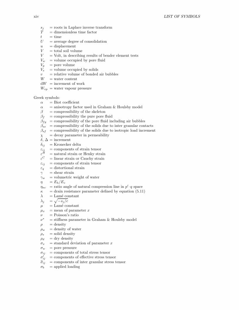
sj = roots in Laplace inverse transformT = dimensionless time factort = timeU = average degree of consolidationu = displacementV = total soil volumeV = Volt, in describing results of bender element testsVw = volume occupied by pore fluidVp = pore volumeVs = volume occupied by solidsv = relative volume of bonded air bubblesW = water contentdW = increment of workWvp = water vapour pressure
Greek symbols:α = Biot coefficientα = anisotropy factor used in Graham & Houlsby modelβ = compressibility of the skeletonβf = compressibility the pure pore fluidβfg = compressibility of the pore fluid including air bubblesβss = compressibility of the solids due to inter granular contactsβsf = compressibility of the solids due to isotropic load incrementχ = decay parameter in permeabilityδ, ∆ = incrementδij = Kronecker deltaεij = components of strain tensorεH = natural strain or Henky strainεC = linear strain or Cauchy strainεij = components of strain tensorεq = distortional strainγ = shear strainγw = volumetric weight of waterη = Eh/Evηnc = ratio angle of natural compression line in p′–q spaceκ = drain resistance parameter defined by equation (5.11)λ = Lame constant
λj =√−sj/c
µ = Lame constantµx = mean of parameter xν = Poisson’s ratioν∗ = stiffness parameter in Graham & Houlsby modelρ = densityρw = density of waterρs = solid densityρd = dry densityσx = standard deviation of parameter xσw = pore pressureσij = components of total stress tensorσ′ij = components of effective stress tensorσij = components of inter granular stress tensorσb = applied loading
xv
τ = shear stressω = air solubility in waterψ = angle of effective stress path, ∆q/∆p′
subscripts:h = horizontalv = verticala = axialr = radialθ = tangentiali = initial0 = value at t = 0
superscripts:u = undrained

xvi LIST OF SYMBOLS
Chapter 1
Scope of research
When designing a foundation for an embankment its influence on its surroundings is often animportant issue. In considering this influence a proper indication of horizontal deformations andhorizontal stresses in the subsoil is needed. Many sediment deposits are deposited in horizontalstrata, so it is to be expected that their mechanical properties in both horizontal directions mightdiffer from their properties in vertical direction. Standard soil sampling produces mainly verticallyretrieved samples. Therefore standard soil investigation gives parameters mainly valid for thevertical direction. In general practice it will take a great effort to retrieve horizontally drilledsamples and this is rarely done. So although it is widely recognized that soft soil might showanisotropic behaviour information on parameters in horizontal direction is scarce.
The options to retrieve information on parameters in the horizontal direction would be increasedif some information on anisotropy could be found from vertically retrieved samples. If alone thelevel of anisotropy could be determined from vertically retrieved samples then for particular casesit could be shown when the subsoil behaves anisotropically and the effort of retrieving horizontalsoil samples is worthwhile.
Anisotropy might be found in all types of soil properties, like permeability, stiffness, strengthetc. This thesis focuses on anisotropy in stiffness. Soil stiffness is an important parameter indescribing the consolidation process of soft soil. In special cases the pore pressure developmentdeviates from the usual transient decay, [57], [22], [41]. This can be explained by a redistributionof stresses. Since the deviation of pore pressure development from the usual transient decay islargely determined by the stiffness parameters it is to be expected that anisotropy influences thisbehaviour. The question arises if this phenomenon can be activated in standard laboratory testingand when measured if pore pressure development can be used for parameter determination.
One type of soft soil that especially is to be expected to behave anisotropically is peat. Peatconsists of mainly organic material. Depending on the degree of humification and the organicorigin, fibres at different scales are present in peat. It is to be expected that if there is a dominantdirection along which the fibres are aligned the peat will show anisotropic behaviour. The reactionof peat when loaded perpendicular to the main fibre direction will be different than when loadedin the main fibre direction.
In discussing anisotropy of peat a distinction can be made between induced anisotropy andstructural anisotropy. Structural anisotropy depends solely on the structure of the material e.g.anisotropy caused by the presence of the fibres. If stiffness is stress or strain dependent an asym-metrical stress or strain distribution might lead to anisotropy in stiffness. This type of anisotropyis known as induced anisotropy. For induced anisotropy anisotropic behaviour is a consequence ofthe loading applied in the past. Since peat is a soft, compressible material it might show inducedanisotropy besides structural anisotropy.
1
2 CHAPTER 1. SCOPE OF RESEARCH
So two questions emerge:
- is it possible to establish the influence of anisotropy in the consolidation behaviour in standardlaboratory testing?
- if pore pressure measurements reveal information on anisotropy can they be used to unravelthe nature of anisotropy of peat?
Before answering these questions two important restrictions are made. The first involves thetype of anisotropy. It is assumed that in describing the anisotropy in stiffness of peat there is oneaxis of symmetry. This means that when e.g. this axis corresponds to the vertical the stiffnessparameters in the horizontal plane are independent from the stiffness in the vertical direction.This type of anisotropy is known as cross–anisotropy. So for peat it is assumed that the fibresare mainly aligned in one plane. Within this plane there is no dominant fibre direction. For abetter understanding it will often be assumed that this plane is the horizontal plane. However thisassumption is not necessary.
The second restriction involves material behaviour. It is widely recognized that a proper de-scription of soft soil behaviour includes plasticity. This holds especially for large deformations.For small deformations and over–consolidated material conditions in engineering practice soil be-haviour is often described by elastic material behaviour using equivalent elastic parameters thatinclude some plasticity. In the following chapters it is assumed that a linear elastic material modelcan be used to describe behaviour of peat during consolidation. As a consequence deformations areassumed to be small during consolidation and the tested soil is over–consolidated. The main reasonfor assuming elastic material behaviour is that analytical solutions for the relevant phenomenoncan be derived. These analytical solutions give an understanding in the basic nature of the studiedphenomena. Once understanding the basic features the analysis can be extended to plastic soilbehaviour.
To answer the two questions stated above chapter 2 starts with a discussion on the stiffness ofthe individual soil constituents, solids and pore fluid in relation to the bulk stiffness parameters.Chapter 3 gives a mathematical description of linear elastic cross–anisotropic material behaviour.Chapter 4 gives a literature review on the topic of parameter assessment for a cross–anisotropicsoil model. This chapter shows some measurement results presented in literature and discussesthe physical boundaries for individual parameters or group of parameters. Chapter 5 discussesinfluence of stress redistribution on the consolidation behaviour of soft soil, starting with a liter-ature overview. The second part of chapter 5 presents several analytical solutions in which theinfluence of cross–anisotropic soil stiffness to the pore pressure development during consolidationplays a role. The analytical solutions clearly show that anisotropy in stiffness influences the porepressure development for a conventional cylindrical soil sample. Chapter 6 shows measurementson peat conducted on conventional samples. Chapter 7 illustrates some size effects by discussingmeasurements on a large scale triaxial test. Finally chapter 8 gives three illustrations showingthe practical implications for some aspects of the derived theory. The mathematical derivationsof the solution for the different consolidation problems derived in the main text are presented inappendices.

Chapter 2
Compressibility of soil constituents
2.1 Parameters of compressibility
A soil volume contains solids and pores. Since pores might be filled by fluid and/or gas, a soilvolume might contain three constituents, solids, pore fluid and pore gas. When describing themechanical behaviour of soil the compressibility of the individual constituents play an essentialrole at micro level, while at macro level a bulk modulus is used. In soil mechanics solids (or grains)are often assumed to be incompressible. This assumption seems to hold for materials like sandand clay. Peat and organic clay however contain organic material. It might be possible that theorganic fibres contain air pockets that are not connected to the pores. Such fibres can be seen asa compressible solid. A possible compressibility of the solids influences the mechanical behaviourof soil in several ways, three of which are explicitly considered:
- The stress dependency of the compressibility
- The concept of effective stress
- The Skempton B–factor in an undrained triaxial test
The first two items are used to illustrate the importance of the assumption of incompressible solids.The third item is used to validate measurement data that are presented in detail in section 6.5.
In chapters 2, 3, 4, 6, 7 and 8 the general sign convention is adopted in which all stress andstrain are chosen positive for tension and negative for compression. When discussing analyticalsolutions to the consolidation problem chapter 5 uses, in contrast to the general sign convention,a positive sign for pore pressure. As explained in section 5.3 this sign convention makes directcomparison to solutions presented in literature possible.
2.2 Compressibility of the pore fluid, βfg
The degree of saturation is defined as ratio of pore volume occupied by pore fluid and total porevolume:
Sr =VwVp
(2.1)
Sr = degree of saturationVw = volume occupied by the pore fluidVp = pore volume
3

4 CHAPTER 2. COMPRESSIBILITY OF SOIL CONSTITUENTS
.............................................................................................................................................................................................................................................................................................. ...................
.....
.....
.....
.....
.....
.....
.....
.....
.....
.....
.....
.....
.....
.....
.....
.....
.....
.....
.....
.....
.....
.....
.....
.....
.....
.....
.....
.....
.....
.....
.....
.....
.....
.....
.....
.....
.....
.....
.....
.....
.....
.....
.....
.....
.....
.....
.....
.....
.....
.....
.....
.....
.....
.....................
...................
Vp
σw
..........................................................................................................................................................................................................................................................................................................................................................................................
.................................................................................................................................................................................................................
..................................................................................................................................................................................
dVp
dσw
Figure 2.1: Definition of compressibility
For Sr = 1 the soil is completely saturated. Thenall pores are filled with water and no gas phase ispresent. For Sr = 0 the soil is dry and no pore fluidis present. For unsaturated soils, 0< Sr < 1 a furthersubdivision is possible. For a small amount of gas,the gas phase consists of individual bubbles presentin the pore fluid. According to Fredlund & Rahardjo[31] this phase is reached for Sr = 0.90. For Sr <0.80 a continuous gas-phase is present. In the tran-sition zone both occur. For a continuous gas-phasethe motion of the pore fluid is considerably hinderedby the presence of the gas. In the following theseconditions are excluded and it is assumed that Sr >0.85. The pore fluid–gas bubble mixture is then described as a fluid in which the properties of gasbubbles and original fluid are incorporated. Under the assumption of constant temperature figure2.1 defines the pore fluid compressibility βfg due to a pore pressure increment dσw .
βfg = − 1
Vp
dVpdσw
(2.2)
The presence of the gas bubbles mainly involves the compressibility of the fluid. As indicatedby several authors a small number of bubbles in the pore fluid reduces the stiffness of the porefluid considerably, [6], [65] and [31]. Barends [6] gives an extended description of the stiffness of apore fluid–gas bubble mixture:
βfg = βf+
[1 − (1 − ω)Sr]2
Sr
(1 − ω) [1 − (1 − ω)Sri]
[σwi −Wvp +
2σ
ri
]− 2σ
3ri[1 − (1 − ω)Sr]
2 3
√(1 − Sri − v)
(1 − Sr − v)4
(2.3)
In which:
βf = compressibility of the pure pore fluidω = air solubility in waterSri = initial degree of saturationσwi = initial pore pressureWvp = water vapour pressureσ = fictitious water-air surface tension of the gas-fluid mixtureri = initial free air bubble radiusv = relative volume of bonded air bubbles
As the gas-bubbles have a relative large compressibility the volume occupied by air bubblesdecreases when the fluid pressure σw increases, leading to an increase in Sr. Following Barends[6], the relation between σw and Sr is given by:
σw = Wvp −2σ
ri
3
√(1 − Sri − v)
(1 − Sr − v)+
[1 − (1 − ω)Sri]
[σwi −Wvp + 2
σ
ri
]
[1 − (1 − ω)Sr)(2.4)
Figure 2.2 illustrates equations (2.3) and (2.4). The equations are elaborated for two values ofthe initial degree of saturation, Sri = 0.85 and 0.92. The coefficients in equation (2.3) are takenfrom [6], with p0 the atmospheric pressure;

2.3. COMPRESSIBILITY OF THE SOLID PARTICLES 5
0 5 10 15
σw/p0
−0.5
0.0
0.5
1.0
1.5
2.0
σw = σwc............................................................................
.............
...................
.........................................................................
.....
.....
.....
....
......
......
......
....................................................................................
......
......
......
......
.......
.....
.....
.
.....
.
.....
.
.....................................................................................................................................
....................................................................................................................................................................
βfg [ ×10−6 m2/N]
0.84 0.88 0.92 0.96 1.00
Sr
−0.5
0.0
0.5
1.0
1.5
2.0
βfg [ ×10−6 m2/N]
..............................................................................................................................................................................
............
................................................................................................................................
......
Sri = 0.92Sri = 0.85
Figure 2.2: βfg vs Sr and βfg vs σw/p0, after Barends [6]
ω = 0.02p0 = 105 N/m2
Wvp = 1000 N/m2
σ/ri = 10 000 N/m2
v = 10−7
βf = 10−9 m2/N
As explained by Barends [6] an increase in σw leads to an increase in Sr according to equation(2.4). At some critical pressure σwc the air bubbles are no longer stable and collapse. Then thegas phase is completely dissolved in the pore fluid and air bubbles are no longer present. Whenreaching σwc equation (2.3) predicts a sudden jump in βfg. This leads to a singular point inequation (2.3) depicted by a vertical line in figure 2.2. The negative values for βfg presented infigure 2.2 have no physical meaning but are a consequence of the singular point at σw = σwc.Figure 2.2b shows that for σw = σwc the stiffness of the pore fluid jumps from βfg for σw < σwcto βf for σw > σwc. Figure 2.2b shows also that the value for σwc depends on Sri. Note, that fora large Sri complete saturation is found at a smaller pore pressure increase while for a lower Sri alarger stress increment is required. So, for Sri = 0.85 complete saturation is found when σwc/p0 ≈8.4 while for Sri = 0.92 is found σwc/p0 ≈ 4.6 . The sudden jump in the stiffness of the pore fluidat the critical pressure is also found in figure 2.2a when Sr reaches 1.0. Only for Sr = 1.0 thecompressibility of the fluid-gas mixture is equal to the compressibility of the pure fluid. Figure 2.2illustrates the reasoning of using a back–pressure to improve Sr in standard triaxial testing.
2.3 Compressibility of the solid particles
2.3.1 Compression due to isotropic loading, βsf
An individual solid particle will face an isotropic stress caused by the surrounding pore fluid. Asexplained by Verruijt [77], despite the presence of contact points, where the individual grains toucheach other, the pressure from the pore fluid is considered to act around the entire surface. Thecompressibility of the solid particles under an isotropic stress increment is indicated by βsf :
βsf = − 1
Vs
dVsdσw
(2.5)
6 CHAPTER 2. COMPRESSIBILITY OF SOIL CONSTITUENTS
With Vs the volume of the solid material and Ms the mass of the solid material, ρs is defined byρs = Ms/Vs. Since Ms is independent of dσw the following is found:
dMs
dσw= 0 → d (ρsVs)
dσw= 0 → dρs
ρsdσw= − dVs
Vsdσw
and with equation (2.5) it follows that:
βsf =dρsρsdσw
(2.6)
2.3.2 Compression due to inter granular contacts, βss
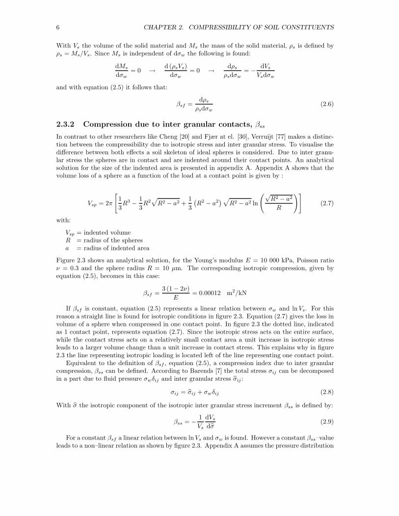
In contrast to other researchers like Cheng [20] and Fjær at el. [30], Verruijt [77] makes a distinc-tion between the compressibility due to isotropic stress and inter granular stress. To visualise thedifference between both effects a soil skeleton of ideal spheres is considered. Due to inter granu-lar stress the spheres are in contact and are indented around their contact points. An analyticalsolution for the size of the indented area is presented in appendix A. Appendix A shows that thevolume loss of a sphere as a function of the load at a contact point is given by :
Vsp = 2π
[1
3R3 − 1
3R2√R2 − a2 +
1
3
(R2 − a2
)√R2 − a2 ln
(√R2 − a2
R
)](2.7)
with:
Vsp = indented volumeR = radius of the spheresa = radius of indented area
Figure 2.3 shows an analytical solution, for the Young’s modulus E = 10 000 kPa, Poisson ratioν = 0.3 and the sphere radius R = 10 µm. The corresponding isotropic compression, given byequation (2.5), becomes in this case:
βsf =3 (1 − 2ν)
E= 0.00012 m2/kN
If βsf is constant, equation (2.5) represents a linear relation between σw and lnVs. For thisreason a straight line is found for isotropic conditions in figure 2.3. Equation (2.7) gives the loss involume of a sphere when compressed in one contact point. In figure 2.3 the dotted line, indicatedas 1 contact point, represents equation (2.7). Since the isotropic stress acts on the entire surface,while the contact stress acts on a relatively small contact area a unit increase in isotropic stressleads to a larger volume change than a unit increase in contact stress. This explains why in figure2.3 the line representing isotropic loading is located left of the line representing one contact point.
Equivalent to the definition of βsf , equation (2.5), a compression index due to inter granularcompression, βss can be defined. According to Barends [7] the total stress σij can be decomposedin a part due to fluid pressure σwδij and inter granular stress σij :
σij = σij + σwδij (2.8)
With σ the isotropic component of the isotropic inter granular stress increment βss is defined by:
βss = − 1
Vs
dVsdσ
(2.9)
For a constant βsf a linear relation between lnVs and σw is found. However a constant βss–valueleads to a non–linear relation as shown by figure 2.3. Appendix A assumes the pressure distribution

2.3. COMPRESSIBILITY OF THE SOLID PARTICLES 7
0 2000 4000 6000 8000 10000 12000 14000 16000 18000
σw, q0 [kN/m2]
0.0
0.2
0.4
0.6
..........................................................................................................................................................................................................................................................................................................................................................................................................................................................................
......................
ln(Vs/Vs0)
.................................................................
.............
.........
.......
......
.........................................................................................
.....
......................................................................................................................................................
..............................
.......................
........................................................................................................................................................................................................................................................................................................................................................
................
.......................................................................................................................
...........................
...........................................................................................................................................................................................................................................................................................................................................
..............
pore fluid pressure
1 contact point
4 contact points
6 contact points
A
B
B•
23q0a
.....................................................................................................................................................
...........................................................................
.....
.....
.....
.....
.....
.....
.....
....................
...................
.........................................
.....
.....
....
.....
.....
.....
....
....................................................... ................... ..........................................................................
....................
....................
....................
....................
.....
.....
................................
......................................................................................................................................................................................A•
σw.......................................................
...................
.......................................................
..........................................................................
............................................................................................. .......
................................................................... .........
..................
...............................................
..........................
................................................
..........................................................................
..........................................................................
.....
.....
.....
.....
.....
.....
.....
....................
...................
.......................................................
...................
.......................................................
..........................................................................
..........................................................................
..........................................................................
.............................................
.........................................................................
.................................................
..........................................................................
.....
.....
.....
.....
.....
.....
.....
....................
...................
.......................................................
...................
.......................................................
...................
.......................................................
...................
.......................................................
...................
.......................................................
...................
.......................................................
................... .......................................................
................... .......................................................
...................
.......................................................
.....
.....
.....
....
.......................................................
.....
.....
.....
..............................................
.............
...................
....................................................
....................................................................
................................................................................
......................
....................................................... ................
...
....................................................... ...................
.........................................
.....
.....
....
.....
.....
.....
....
...
...
............
..........................................................................................
.................................................
..............................
......
.................................................
..............................
......
.....
.....
.................................
..................................................................... ............................................................................................................................................................................................................................
.........................................
.....
.....
....
.....
.....
.....
....
........................................
.....
.....
....
.....
.....
.....
....
....................................
.....
.....
....
.....
.....
.....
...............................................
.....
.....
.....
....
........................................
.....
.....
....
.....
.....
.....
....
....................................
.....
.....
....
.....
.....
.....
...............................................
.....
.....
.........
.....................................................................................................
...............
2a
.................................................................................................
...............
q0
Figure 2.3: Stress–strain curve for an isotropic stress σw, condition A and inter granular stress q0,condition B
in the contact area, with radius a, to be semi–spherical with q0, the maximum pressure at the centreof the area. Appendix equation (A.5) gives a linear relation between q0 and a. When a increases,the part of the sphere that is lost due to denting of the sphere increases disproportionally, leadingto a non–linear relation between a and Vsp.
The grains in a skeleton will usually have more than one contact point. Considering only smallvolume changes it can be assumed that the individual contact points do not interact. So for agrain having 4 contact points the total volume loss can be estimated by 4 times the volume lossat one contact point. In figure 2.3 the loss in volume is given for 4 and 6 contact points.
The tangent of the isotropic compression line gives βsf . The tangent of the inter granularcompression lines gives a value for βss. From figure 2.3 the difference between βss and βsf isevident. For low values of q0 the volume loss of the solid particles due to contact stress can beneglected. When q0 increases βss increases and may finally exceed βsf .
Equivalent to the equations (2.5) and (2.6) a definition of βss and a relation between βssandρs can be found.
dMs
dσ= 0 → d (ρsVs)
dσ= 0 → dρs
ρsdσ= − dVs
Vsdσ
with equation (2.9):
βss =dρsρsdσ
(2.10)
Under the assumption that interaction between compression due to an isotropic fluid pressure andinter granular stress is negligible the density as a function of σw and σ is found by a summationof both the individual density changes:
dρsρs
= βsfdσw + βssdσ (2.11)

8 CHAPTER 2. COMPRESSIBILITY OF SOIL CONSTITUENTS
Or expressed in terms of change in Vs:
dVsVs
= −βsfdσw − βssdσ (2.12)
And expressed in terms of the bulk volume, with n representing porosity:
dVsV
= − (1 − n) (βsfdσw + βssdσ) (2.13)
2.4 Compressibility of the skeleton, β
The total volume change of a soil mass involves a rearrangement of the solid particles. This iscaused by sliding, rolling or crushing of the grains. The compressibility which accounts for theseeffects as well as for the inter granular compression is denoted by β. Since the stress exerted bythe pore fluid on the grains is an isotropic stress, sliding, rolling and crushing of the grains isinfluenced by the inter granular stress only.
Terzaghi, [71] defines the effective stress, indicated by σ′, as that part of the total stress tensorleading to deformation of the skeleton. Equivalent to equation (2.5) compressibility of the skeletonβ is defined, with dσ′ the isotropic effective stress increment, by:
β = − 1
V
dV
dσ′(2.14)
The fact that β includes compression of the individual grains as well as a reduction in porevolume can be visualised by considering a compression test on a dry sample. For these conditionsthe grains only face increments of inter granular stress, so ∆σ = ∆σ = ∆σ′. From a reduction involume of the solids it can then be found, using equation (2.9):
∆Vs = ∆(1 − n)V = (1 − n)∆V − V∆n
(1 − n)∆V = ∆Vs + V∆n
∆V = −βss∆σ′V + V∆n
1 − n
With equation (2.14) it can be found:
β = βss −∆n
(1 − n)∆σ′
Since ∆n/∆σ′ < 0 it is found β > βss. For most soils βss is at least one order magnitude smallerthan ∆n/∆σ′ and hence, β ≈ −∆n/∆σ′.
2.5 The effective stress concept
By definition the effective stress, indicated by σ′, is that part of the total stress tensor whichcontrols the deformation of the skeleton. Terzaghi [71] introduced the concept of effective stressin 1925. Biot extended the definition for compressible solids [12], [13] and [14] and shows that theeffective stress tensor is defined by:
σ′
ij = σij − ασwδij , α = 1 − βsfβ
(2.15)
In equation (2.15) the coefficient α represents the Biot factor. In soil mechanics the solidparticles are usually assumed to be incompressible. For these conditions βsf reduces to 0, leading

2.6. SKEMPTON B–FACTOR 9
to α = 1. For incompressible solids, α = 1, the Terzaghi formulation of effective stress is found.For compressible solids α is smaller than 1.
Since the effective stress is defined as that part of the total stress that causes skeleton defor-mation, the pore pressure of a soil type with compressible solids partly contributes to the skeletondeformation. According to equation (2.15) the part of the pore pressure that contributes to theeffective stress is given by βsfσw/β.
2.6 Skempton B–factor
Skempton, [65], introduces the B–factor as a function of pore water stiffness Kw and skeletonstiffness K. With K = 1/β and Kw = 1/βfg, the Skempton B–factor is represented by:
B =1
nK
Kw
+ 1=
1
nβfgβ
+ 1
(2.16)
The Skempton B–factor is an important parameter to validate the degree of saturation inlaboratory tests. As shown by Verruijt [77] a reformulation of the Skempton B–factor can befound using βss, βsf , βfg and β. For initial, undrained, conditions no dissipation of pore watertakes place. So when loading the total volume change equals the summation of pore volumereduction and solid volume reduction:
∆V = ∆Vp + ∆Vs
Using equations (2.2), (2.13) and (2.14) and definitions (2.8) and (2.15) a more general expressionfor the B–factor is found:
B =dσwdσ
=β − (1 − n)βss
β − (1 − n)βss − nβsf + nβfg=
1
1 +n (βfg − βsf )
β − (1 − n)βss
(2.17)
In equation (2.17) the compressibility of the solids is incorporated by the parameters βss andβsf . It can easily be verified that neglecting the compressibility of the solid particles, βsf = βss =0, reduces equation (2.17) to (2.16).
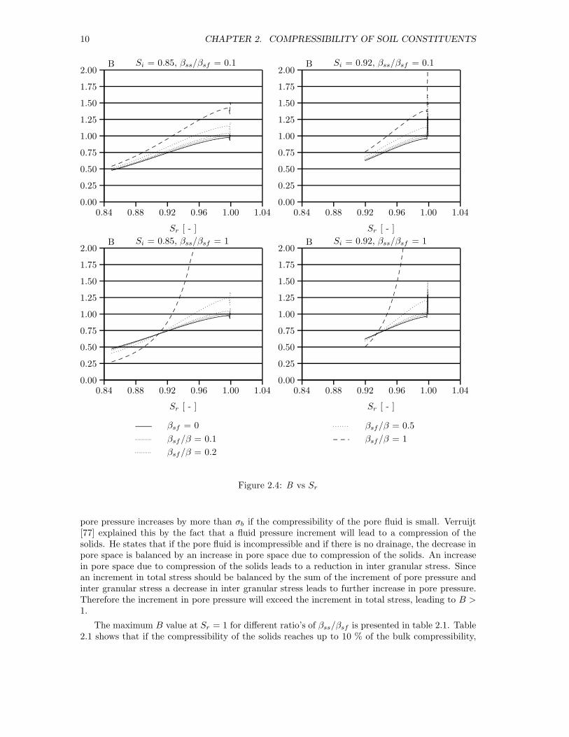
Equation (2.3) gives the stiffness of the pore fluid as a function of the degree of saturation, Sr.So equations (2.17) and (2.3) can be used to draw graphs of the B–factor versus Sr. Figure 2.4shows these graphs for different values for βss/βsf , βsf/β and Sri. By definition β includes βss,so β ≥ βss. Since negative values for α are not expected for soil, β is also limited by βsf .
Figure 2.4 shows a considerable reduction in the B–factor for a small amount of air bubbles.For Sr = Sri = 0.85 the B–factor = 0.5 while for Sr = 1.0 the B–factor equals to 1.0. The largefluctuation in B–factor corresponds to the values presented in literature. Skempton presented mea-surements of the B–factor versus Sr [65], where even lower values for the B–factor are presented,approximately 0.25 for Sr = 0.85. In [65] the initial degree of saturation and the total pressureat which the tests are conducted are not presented. Therefore, equation (2.3) can not be used toreproduce the measurements to explain the difference between test results of [65] and figure 2.4.
Figure 2.4 shows in the lower graphs that the line representing βsf = β deviates strongly fromthe other curves. This is explained by equation (2.17). The curve represents βss = βsf = β andequation (2.17) is then reduced to B = nβ/βfg. Since βfg is strongly influenced by Sr and evenreduces to 0 when Sr reaches 1.0. B grows to infinity for Sr reaching 1.
Figure 2.4 indicates that if βsf is small in comparison to β the influence of βsf on the B–factor isnegligible. When βsf is of the order in magnitude of β the B–factor tends to increase for increasingβsf . It is remarkable that for compressible solids the B–factor becomes larger than 1.0. This meansthat when a soil skeleton, which consists of compressible solids, is loaded by a load equal to σb, the
10 CHAPTER 2. COMPRESSIBILITY OF SOIL CONSTITUENTS
0.84 0.88 0.92 0.96 1.00 1.04
Sr [ - ]
0.00
0.25
0.50
0.75
1.00
1.25
1.50
1.75
2.00B
...................................
.................................
................................
...............................
..............................
..............................
.................................
..................................
.......................................
...................................................................
....
........
.........
.........
........
........
........
........
........
.........
...........
.................
.......
......
......
......
......
......
......
......
.......
............
.
.
.
.
......
......
.............................
......
..........
.
..
......................
......................
....................................................................................................................................
.................................
.....
.....
.
.........
Si = 0.85, βss/βsf = 0.1
0.84 0.88 0.92 0.96 1.00 1.04
Sr [ - ]
0.00
0.25
0.50
0.75
1.00
1.25
1.50
1.75
2.00B Si = 0.92, βss/βsf = 0.1
............................................................................................................................
...............................
...................................................................................................................................................
...............................
........
..........
..
..
..
..
..
..
..
..
................
......
........
......
......
......
...............................
.............................
.............................
..............................................................................................................
..................................................................
......
0.84 0.88 0.92 0.96 1.00 1.04
Sr [ - ]
0.00
0.25
0.50
0.75
1.00
1.25
1.50
1.75
2.00B Si = 0.85, βss/βsf = 1
...................................
..................................
.................................
...............................
..............................
...............................
...............................
...................................
........................................
................................................................
.....
.......
...........................................
.........
.........
........
........
........
........
........
........
..........
.................
..
.
............
.......
......
......
......
......
......
......
......
......
.........
..........
.........
......
.................................................
...........
......................
........................................................................................................................................................................................................
βsf = 0
βsf/β = 0.1
βsf/β = 0.2
0.84 0.88 0.92 0.96 1.00 1.04
Sr [ - ]
0.00
0.25
0.50
0.75
1.00
1.25
1.50
1.75
2.00B Si = 0.92, βss/βsf = 1
...........................................................................................................................................
......................................
.............................................................................................................................
...............................
........
...........
..
..
..
..
..
..
..
..
..................
.....
.................
......
.......
..................................
.................................
.
.
.......
.....................................................................................................................................................................
........... ........... ...
βsf/β = 0.5
βsf/β = 1
Figure 2.4: B vs Sr
pore pressure increases by more than σb if the compressibility of the pore fluid is small. Verruijt[77] explained this by the fact that a fluid pressure increment will lead to a compression of thesolids. He states that if the pore fluid is incompressible and if there is no drainage, the decrease inpore space is balanced by an increase in pore space due to compression of the solids. An increasein pore space due to compression of the solids leads to a reduction in inter granular stress. Sincean increment in total stress should be balanced by the sum of the increment of pore pressure andinter granular stress a decrease in inter granular stress leads to further increase in pore pressure.Therefore the increment in pore pressure will exceed the increment in total stress, leading to B >1.
The maximum B value at Sr = 1 for different ratio’s of βss/βsf is presented in table 2.1. Table2.1 shows that if the compressibility of the solids reaches up to 10 % of the bulk compressibility,

2.6. SKEMPTON B–FACTOR 11
Table 2.1: Skempton B–factor for compressible solids at Sr = 1βsf/β 0 0.02 0.1 0.2 0.5 1.0
βss/βsf = 0.1 1.00 1.01 1.03 1.06 1.18 1.47βss/βsf = 1.0 1.00 1.01 1.03 1.07 1.30 500 (∞)βss/βsf = 10 1.00 1.01 1.11
the influence of the solid stiffness remains small. The deviation of the B–factor is then 3%.

12 CHAPTER 2. COMPRESSIBILITY OF SOIL CONSTITUENTS

Chapter 3
Cross–anisotropic elasticity
3.1 Hooke’s law for cross–anisotropy
Figure 3.1 visualises a cross–anisotropic material. The discs located in the x–y plane represent theplane of isotropy. The stress and strain in the plane of the discs follow from the disc properties.The stress and strain in the z–direction follow from the properties of the bar. The stress and strainin the x–z and y–z plane follow from the interaction of the bar and discs. For normal stress andstrain the most general description of the normal stress–strain relationship is given by equation(3.1), with a sij a general stiffness matrix.
............................... ...........................................................................................................................................................................................................................................................................................................................................................................................................................................................................................................................
............................................................................................................................................................................................................................................................................................................
.....
.....
.....
.
.....
.....
.....
.
..................................................................................................................................................................................................................................................................................................................................................................................................................................................................................................................
......................................................................................................
.....
.....
.....
.
.....
.....
.....
..............................................................
....................................................................
.....
.....
.....
.....
.....
.....
.....
.....
.....
.....
.....
.....
.....
.....
.....
.....
.....
.....
.
.....
.....
.....
.....
.....
.....
.....
.....
.....
.....
.....
.....
.....
.....
.....
.....
.....
.....
.
............................................................................
............................................................................
.....
.....
.....
.
.....
.....
.....
.
..........................................................................
.....................................
.....................................
.....................................
z
y
x
............. ............. ............. ............. ............. ............. ............. ............. ............. ............. .................... ..................
.....
...
.....
.....
...
.....
.....
...
.....
.....
...
.....
.....
...
.....
.....
...
.....
.....
...
.....
.....
...
.....
.....
...
.....
.....
...
.............
.............
..........................
..........................
..........................
..........................
.............
Figure 3.1: Cross–anisotropic material
εxx = sxxσxx + sxyσyy + sxzσzz
εyy = syxσxx + syyσyy + syzσzz (3.1)
εzz = szxσxx + syzσyy + szzσzz
Note that in equation (3.1) increments of normal stress and normal strain are presented. Forsake of simplicity the δ sign is omitted.
13

14 CHAPTER 3. CROSS–ANISOTROPIC ELASTICITY
According to equation (3.1), if σxx is the only stress active it will provoke strain in each ofthe three principal directions. For εxx is found εxx = sxx σxx. If a linear elastic stress–strainrelationship is considered, it follows that sxx = 1/Ex, where Ex represents the Young’s modulus.In the same way syy and szz can be defined.
With σyy the only active stress gives εyy = syy σyy, with syy = 1/Ey. In [35] the Poisson’s ratiois defined as the ratio of principal strain in two independent directions under uniaxial loading1 :
ε(jj)
ε(ii)= −νij , if σ(ii) = σ, σ(jj) = 0
Again with σyy the only stress acting gives εxx = sxyσyy leading to sxy = - νyx/Ey. Equivalentexpressions for the coefficients syx to szx can be found. Hooke’s law for normal stress and strainbecomes:
εxx
εyy
εzz
=
1
Ex
−νyxEy
−νzxEz
−νxyEx
1
Ey
−νzyEz
−νxzEx
−νyzEy
1
Ez
σxx
σyy
σzz
(3.2)
The stiffness matrix presented in equation (3.2) is symmetrical. In [35] this is proved in thefollowing way. If the normal stress in e.g. x direction is increased from σxx to σxx + dσxx, theincrement of work dW done becomes:
dW = εxxdσxx = (sxxσxx + sxyσyy + sxzσzz) dσxx
Thus:dW
dσxx= sxxσxx + sxyσyy + sxzσzz
∂2W
∂2σxx= sxx;
∂2W
∂σxx∂σyy= sxy;
∂2W
∂σxx∂σzz= sxz
The same holds for a stress increment in the y and z direction, leading to:
∂2W
∂σyy∂σxx= syx; etc.
Since the order of differentiation is immaterial it is found that:
∂2W
∂σxx∂σyy=
∂2W
∂σyy∂σxx; etc.
And therefore:sxy = syx; etc. (3.3)
Combination of equation (3.3) and (3.2) gives in a more general notation:
−νijEi
=−νjiEj
(3.4)
Note that for anisotropic conditions, Ei 6= Ej , leads to νij 6= νji and vice versa. Love in [56] givesa more thorough proof of the symmetry of the elasticity matrix.
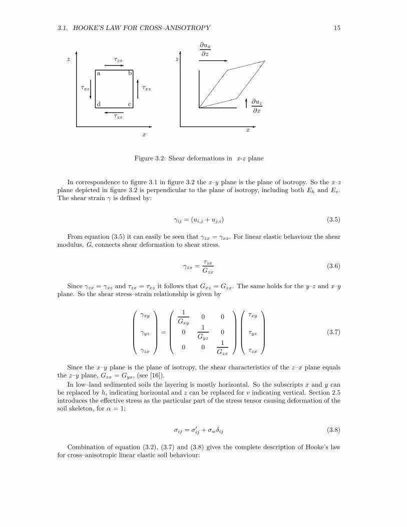
Figure 3.2 shows the shear stress and shear deformations active in the x–z plane. Rotationalequilibrium of plate abcd in figure 3.2 gives τij = τji.
1The subscript (ii) in ε(ii) indicates a cyclic permutation of x, y and z, while εii indicates the summationεxx + εyy + εzz
3.1. HOOKE’S LAW FOR CROSS–ANISOTROPY 15
6
-
�
6
-
?
x
z
τxzτxz
τzx
τzx
a b
cd
-
6
�������
��
���
������
��
��
��
6
-
∂uz∂x
∂ux∂z
x
z
Figure 3.2: Shear deformations in x-z plane
In correspondence to figure 3.1 in figure 3.2 the x–y plane is the plane of isotropy. So the x–zplane depicted in figure 3.2 is perpendicular to the plane of isotropy, including both Eh and Ev.The shear strain γ is defined by:
γij = (ui,j + uj,i) (3.5)
From equation (3.5) it can easily be seen that γzx = γxz. For linear elastic behaviour the shearmodulus, G, connects shear deformation to shear stress.
γzx =τzxGzx
(3.6)
Since γzx = γxz and τzx = τxz it follows that Gxz = Gzx. The same holds for the y–z and x–yplane. So the shear stress–strain relationship is given by
γxy
γyz
γzx
=
1
Gxy0 0
01
Gyz0
0 01
Gzx
τxy
τyz
τzx
(3.7)
Since the x–y plane is the plane of isotropy, the shear characteristics of the z–x plane equalsthe z–y plane, Gzx = Gyz, (see [16]).
In low–land sedimented soils the layering is mostly horizontal. So the subscripts x and y canbe replaced by h, indicating horizontal and z can be replaced for v indicating vertical. Section 2.5introduces the effective stress as the particular part of the stress tensor causing deformation of thesoil skeleton, for α = 1;
σij = σ′
ij + σwδij (3.8)
Combination of equation (3.2), (3.7) and (3.8) gives the complete description of Hooke’s lawfor cross–anisotropic linear elastic soil behaviour:
16 CHAPTER 3. CROSS–ANISOTROPIC ELASTICITY
εxx
εyy
εzz
γxy
γyz
γzx
=
1
Eh
−νhhEh
−νvhEv
0 0 0
−νhhEh
1
Eh
−νvhEv
0 0 0
−νvhEv
−νvhEv
1
Ev0 0 0
0 0 01
Ghh0 0
0 0 0 01
Gvh0
0 0 0 0 01
Gvh
σ′xx
σ′yy
σ′zz
τxy
τyz
τzx
(3.9)
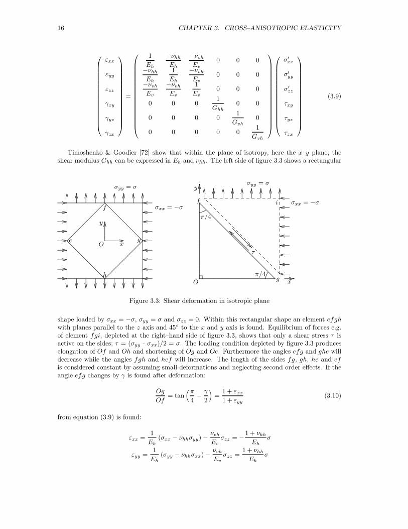
Timoshenko & Goodier [72] show that within the plane of isotropy, here the x–y plane, theshear modulus Ghh can be expressed in Eh and νhh. The left side of figure 3.3 shows a rectangular
.................................................................................................................................................................................................................................................................................................................................................................................................................................................................................................................................................................................................................................................................................................................................................................................................................................................................................................................................................................................................................................................................................................................................................................................... .......
..........................................................................................................................................................................................................................................................................................................................................................................................................................................................................................................................................................................................................................................................................................................................................................................................................................................................................
.....
.....
....
.....
.....
.....
....
.........................................
.....
.....
....
.....
.....
.....
....
.........................................
.....
.....
....
.....
.....
.....
....
.........................................
.....
.....
....
.....
.....
.....
....
.........................................
.....
.....
....
.....
.....
.....
....
.........................................
.....
.....
....
.....
.....
.....
....
.......................................................
.....
.....
.....
....
.........................................
.....
.....
....
.....
.....
.....
....
.........................................
.....
.....
....
.....
.....
.....
....
.......................................................
...................
.......................................................
...................
.......................................................
...................
..........................................................................
..........................................................................
..........................................................................
..........................................................................
.......................................................
...................
.......................................................
..........................................................................
...................
.....
.....
.....
.....
.....
.....
.....
....................
...................
.....
.....
.....
.....
.....
.....
.....
....................
...................
.....
.....
.....
.....
.....
.....
.....
....................
...................
.....
.....
.....
.....
.....
.....
.....
....................
...................
.....
.....
.....
.....
.....
.....
.....
....................
...................
.....
.....
.....
.....
.....
.....
.....
....................
...................
.....
.....
.....
.....
.....
.....
.....
....................
...................
.....
.....
.....
.....
.....
.....
.....
....................
...................
....................................................... ...................
....................................................... ...................
....................................................... ...................
..........................................................................
..........................................................................
..........................................................................
..........................................................................
....................................................... ...................
....................................................... ...................
.....
.....
.....
.....
.....
.....
.....
.....
.....
.....
.....
.....
.....
.....
.....................
...................
..............................................................................................................
Oe
f
g
h
y
x
σyy = σ
σxx = −σ
.............................................................................................................................................................................................................................................................................................................................................................................................................................................................................................................................................................................................................................................................................................................................................................................................................................................................................................................................................................................................................
......................
...........................................................................................................................................
Og
f
π/4
π/4
τ
i
x
yσyy = σ
σxx = −σ
.....
.....
..................
............................
.......................................................................................................................
....................
.......................................................
...................
.......................................................
...................
..........................................................................
..........................................................................
..........................................................................
..........................................................................
..........................................................................
.......................................................
...................
.......................................................
..........................................................................
...................
.....
.....
.....
.....
.....
.....
.....
....................
...................
.....
.....
.....
.....
.....
.....
.....
....................
...................
.....
.....
.....
.....
.....
.....
.....
....................
...................
.....
.....
.....
.....
.....
.....
.....
....................
...................
.....
.....
.....
.....
.....
.....
.....
....................
...................
.....
.....
.....
.....
.....
.....
.....
....................
...................
.....
.....
.....
.....
.....
.....
.....
....................
...................
.....
.....
.....
.....
.....
.....
.....
....................
...................
....................................................... ...................
.....
.....
.....
.....
.....
.....
.....
....................
...................
.....
.....
.
.....
.....
.
.....
.....
.
.....
.....
.
.....
.....
.
.....
.....
.
.....
.....
.
.....
.....
.
.....
.....
.
.....
.....
.
.....
.....
.
.....
.....
.
.....
.....
.
.....
.....
.
.....
...........................................................................................................................................................................
......................
......................
......................
......................
......................
......................
......................
......................
......................
...........
Figure 3.3: Shear deformation in isotropic plane
shape loaded by σxx = −σ, σyy = σ and σzz = 0. Within this rectangular shape an element efghwith planes parallel to the z axis and 45◦ to the x and y axis is found. Equilibrium of forces e.g.of element fgi, depicted at the right–hand side of figure 3.3, shows that only a shear stress τ isactive on the sides; τ = (σyy - σxx)/2 = σ. The loading condition depicted by figure 3.3 produceselongation of Of and Oh and shortening of Og and Oe. Furthermore the angles efg and ghe willdecrease while the angles fgh and hef will increase. The length of the sides fg, gh, he and efis considered constant by assuming small deformations and neglecting second order effects. If theangle efg changes by γ is found after deformation:
Og
Of= tan
(π4− γ
2
)=
1 + εxx1 + εyy
(3.10)
from equation (3.9) is found:
εxx =1
Eh(σxx − νhhσyy) −
νvhEv
σzz = −1 + νhhEh
σ
εyy =1
Eh(σyy − νhhσxx) −
νvhEv
σzz =1 + νhhEh
σ

3.2. BOUNDING VALUES 17
Equation 3.10 and small value for γ gives:
tan(π
4− γ
2
)=
tan(π
4
)− tan
(γ2
)
1 + tan(π
4
)tan
(γ2
) =1 − γ
2
1 +γ
2
substitution gives:
γ =2 (1 + νhh)
Ehτ (3.11)
Equation (3.11) defines the shear modulus in horizontal plane, here the plane of isotropy, by:
Ghh =Eh
2 (1 + νhh)(3.12)
As shown by [16] five parameters suffice to describe cross-anisotropy. The number of indepen-dent parameters used in the matrix of equation (3.9) equals five:
Eh = Young’s modulus in horizontal directionEv = Young’s modulus in vertical directionνvh = Poisson’s ratio for horizontal strain due to vertical strainνhh = Poisson’s ratio for horizontal strain due to horizontal strainGhv = Shear modulus in vertical plane, equals Gvh
3.2 Bounding values
Although the five parameters presented in the previous section are independent they need to fulfilsome requirements. De Josselin de Jong, [40] and Pickering [61] give a clear analysis of the boundingvalues for the five parameters. Since these analyses provide a valuable insight in the behaviour ofcross-anisotropic materials the main points of these analyses are reported in this section. Fromequation (3.9) an expression for the volumetric strain e can be derived:
e = εii =
(1
Eh− νhhEh
− νvhEv
)(σ′
xx + σ′
yy + σ′
zz
)+
(1
Ev− νvhEv
− 1
Eh+νhhEh
)σ′
zz (3.13)
De Josselin de Jong states that compressive stress should lead to compression and requires bothterms of the right-hand side of equation (3.13) to be positive. Pickering does not use this re-quirement and finds for exceptional conditions material behaviour, which expands under axialcompression. Pickering claims this as an option to model dilatancy by linear elastic materialbehaviour. Since the Pickering analysis is more general, it is followed in this section.
With equation (3.9) εij = Cijklσ′kl the strain energy per unit volume is expressed by dW =
1/2σ′ij Cijkl σ
′
kl. From thermodynamic requirements it follows that dW ≥ 0. Pickering states thatthis requirement is fulfilled when all principal minors of matrix Cijkl are positive. The principal

18 CHAPTER 3. CROSS–ANISOTROPIC ELASTICITY
minors of Cijkl are:
C1 =1
Eh
C2 =1
E2h
(1 + ν2
hh
)
C3 =1
E2v
(EvEh
− ν2vh
)
C4 =1
E2vEh
[EvEh
(1 − νhh) − 2ν2vh
](1 + νhh)
C5 =C3
Ghh=
2C3 (1 + νhh)
Eh
C6 =C5
Gvh
C1 to C6 are all positive if:Eh, Ev, Gvh ≥ 0
νhh ≥ −1
EvEh
(1 − νhh) − 2ν2vh ≥ 0
(3.14)
The third condition of (3.14) also gives the upper bound for νhh. Rewriting gives:
EvEh
(1 − νhh) ≥ 2ν2vh
Since ν2vh ≥ 0 and according to the first condition of (3.14) Eh, Ev ≥ 0 follows, (1 − νhh) ≥ 0,
νhh ≤ 1. Note that in conditions (3.14) νhv is not an independent parameter, since equation (3.4)relates νhv to Ev/Eh and νhv. Pickering, [61], uses νhv instead of νvh and finds for minor C4 theexpression:
C4 =1
E3h
[EhEv
(1 − νhh) − 2ν2hv
](1 + νhh)
which with C4 ≥ 0 gives the condition:
EhEv
(1 − νhh) − 2ν2hv ≥ 0 (3.15)
Figure 3.4 shows condition (3.15) in combination to the first and second condition given by(3.14). They are fulfilled if the state is within or on the envelope shown.
Isotropic materials do not show distortion under an isotropic load. Figure 3.4 shows that thereis a combination of stiffness parameters for which a cross–anisotropic material also does not distortunder an isotropic load. This type of behaviour is found when ε(ii) = ε(jj) under an isotropic stress,σ′
(jj) = σ′ and τij = 0. From equation (3.9) with equation (3.4) follows:
εxx = εyy = εzz =
(1
Eh− νhhEh
− νvhEv
)σ′ =
(−2
νvhEv
+1
Ev
)σ′
EhEv
− 1 = νhv − νhh
(3.16)
A material that fulfils equation (3.16) does not show distortion under an isotropic load and viceversa no volume change when loaded such that the isotropic load remains 0. The triangle ABC infigure 3.4 represents this type of material, for which volumetric strain and distortional strain areuncoupled. Isotropic materials are a part of this group of materials, which are represented by the

3.3. STRESSES 19
............................................................................................................................................................................................................................................................................ ...................
.....
.....
.....
.....
.....
.....
.....
.....
.....
.....
.....
.....
.....
.....
.....
.....
.....
.....
.....
.....
.....
.....
.....
.....
.....
.....
.....
.....
.....
.....
.....
.....
.....
.....
.....
.....
.....
.....
.....
.....
.....
.....
.....
.....
.....
.....
.....
.....
.....
.....
.....
.....
.....
.....
.....
.....
.....
.....
.....
.....
.....
.....
.....
.....
.....
.....
.....
.....
.....
.....
.....
....................
...................
..................................................................................................................................................................................................................................................................
...................
.........................................................................................................................................................................................................................................................................................................................................................
................................................................................................................................................................................................................................................................................................................................................
......................................................................................................................................................................................................................................................................................................................................
..........................................................................................................................................................................................................................................................................................................................
.....
......
......
.....
......
......
.....
......
......
......
.....
......
......
.....
......
.....
.....
.....
.....
.....
.....
.....
.....
.....
.....
.....
.....
.....
......
.....
.....
.....
.....
.....
.....
.....
.....
.....
.....
.....
.....
.....
......
.....
.....
.....
.....
.....
.....
.....
.....
.....
.....
.....
.....
.....
......
.....
.
............................................
..............................
..........................
...........................................................................................................................
........................................................
...............................
.............................
.............................
............................
...........................
..........................
...................
................................................................................
...................................
................................
...............................
.............................
.............................
............................
........................
.................................................................................................
........................................
..................................
..................................
..............................
...............................
.............................
......................................................................
..............................................
........................................
...................................
..................................
...............................
...............................
..............................
.............
.....................................................................................................................
.....
.....
.....
.....
.....
.....
.....
.....
.....
.....
.....
.....
.....
.....
.....
.....
.....
.....
.....
.....
.....
.....
.....
.....
.....
.....
.....
.....
.....
.....
.....
.....
.....
.....
.....
.....
.....
.....
.....
.....
.....
.....
.....
.....
.....
.....
.....
.....
.....
.....
.....
.....
.....
.....
.....
.....
.....
.....
.....
.....
.....
.....
.....
.....
.....
.....
...................
..............
...........
...........
....................................................................................................................................
......................
...........
...........
.............................................................................................................................................
......................
...........
...............................................................................................................................................
...........
.................................................................................................................................................................
..................................................................
.....
.........................................................
..................................................
.....
.......................................
........................................................
................................................................................
................................................................................................................
...........................................................................................................................................
...............................................................................................................................................................
0.5
1
2
3
4
EhEv
-1-0.5
00.5
1
νhv
EhEv
νhh
............................................................................................................................................................................................................................................................................ ...................
.....
.....
.....
.....
.....
.....
.....
.....
.....
.....
.....
.....
.....
.....
.....
.....
.....
.....
.....
.....
.....
.....
.....
.....
.....
.....
.....
.....
......................
...................
..................................................................................................................................................................................................................................................................
...................
.........................................................................................................................................................................................................................................................................................................................................................
................................................................................................................................................................................................................................................................................................................................................
......................................................................................................................................................................................................................................................................................................................................
..........................................................................................................................................................................................................................................................................................................................
.....
......
......
.....
......
......
.....
......
......
......
.....
......
......
.....
......
.....
.....
.....
.....
.....
.....
.....
.....
.....
.....
.....
.....
.....
......
.....
.....
.....
.....
.....
.....
.....
.....
.....
.....
.....
.....
.....
......
.....
.....
.....
.....
.....
.....
.....
.....
.....
.....
.....
.....
.....
......
.....
.
........................................................
...............................
.............................
.............................
............................
...........................
..........................
...................
.....
...............................................................................................................................................................................................................................................................
......................................................................................................................................................................................................................................................................................................................................................................................................................................................................................................................................................................................................................................................................................................................................................................................................................................................................................................................................................
......................................................
...................
..............
...........
...........
....................................................................................................................................
........................................................
................................................................................................................
...........................................................................................................................................
...............................................................................................................................................................
Eh/Ev = 1
νhv
EhEv
νhh
• A
•B
•C
•D
Figure 3.4: Bounding values for anisotropic linear elastic parameters after [61]
line CD, Eh/Ev = 1, νhh = νhv. Since Ghv is an independent parameter an anisotropic materialcan still be represented by the line CD.
From equation (3.9) it is found that the strain energy for isotropic loading, σ′
(ii) = σ′, τij = 0,is given by:
dW =1
2Eh
[(1 − 4νvh)
EhEv
+ 2 (1 − νhh)
]σ2
Constant volume deformation requires dW = 0 with νvh = νhvEv/Eh leading to:
EhEv
+ 2 − 4νhv − 2νhh = 0 (3.17)
The intersection with the third condition given by equation (3.14) and (3.15) yields:
νhv =1
2
EhEv
, νhh = 1 − 1
2
EhEv
The intersection produces a straight line although the shape presented by figure 3.4 is stronglycurved. In figure 3.4 the line AB represents the intersection. In soil mechanics constant volumedeformations are found when soil behaves undrained which is further discussed in section 4.3.2.
3.3 Stresses
Any deformation of a soil volume can be expressed in terms of volumetric strain and distortionalstrain. A familiar way to express stress in terms of strain uses the Lame constants. For an isotropiclinear elastic material is found:
σ′
ij = λeδij + 2µεij (3.18)
In which λ and µ are known as Lame constants:
λ = K +2
3G =
νE
(1 + ν) (1 − 2ν), µ = G =
E
2 (1 + ν)

20 CHAPTER 3. CROSS–ANISOTROPIC ELASTICITY
For a cross–anisotropic material stress can be expressed into strain in an equivalent manner. Inliterature references up to now are not known to the author. The complete derivation is presentedin appendix B.
σ′
xx = Ae+ 2Ghhεxx +Bεzz
σ′
yy = Ae+ 2Ghhεyy +Bεzz
σ′
zz = (A+B) e+Dεzz
τxy = Ghhγxy
τyz = Gvhγyz
τzx = Gvhγzx
(3.19)
with:
A =νhhEhEv + ν2
vhE2h
(1 + νhh) (Ev (1 − νhh) − 2Ehν2vh)
B =EhEv (νvh (1 + νhh) − νhh) − ν2
vhE2h
(1 + νhh) (Ev (1 − νhh) − 2Ehν2vh)
D =E2v (1 − νhh) − EhEvνvhEv (1 − νhh) − 2Ehν2
vh
Ghh =Eh
2 (1 + νhh)
Note that for isotropic conditions, Eh = Ev = E, Ghh = Gvh = G and νhh = νvh = ν is found:A = νE/[(1 + ν)(1 − 2ν)] = λ, B = 0 and D = 2G = 2µ and equation (3.19) reduces to (3.18).Equation (3.19) gives a 5–parameter model which is in agreement with the requirements for across-anisotropic model according to section 3.1.
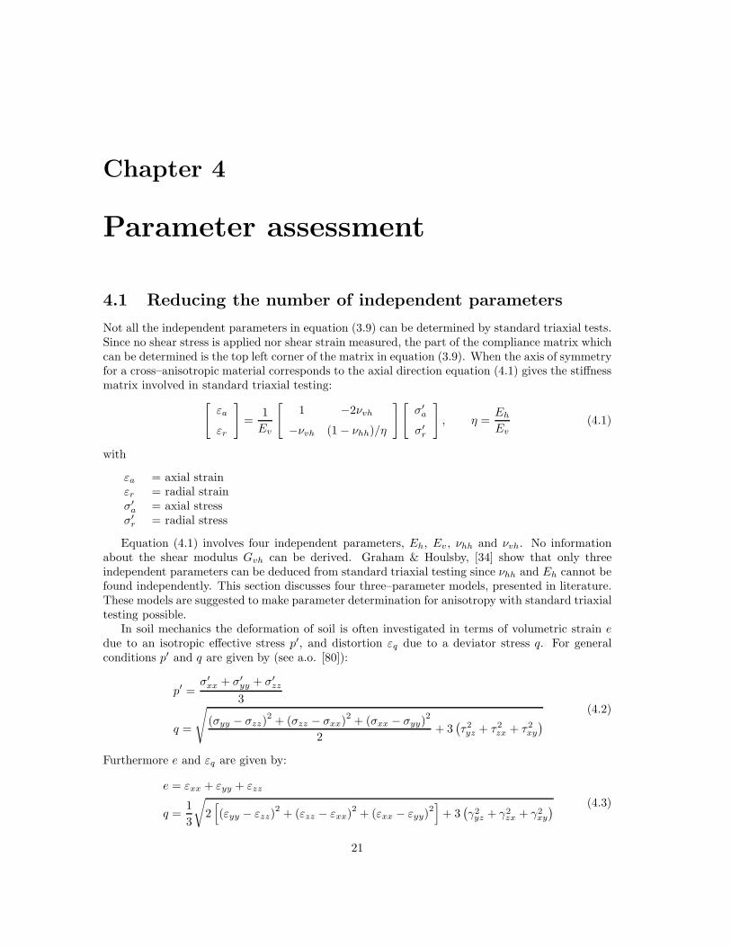
Chapter 4
Parameter assessment
4.1 Reducing the number of independent parameters
Not all the independent parameters in equation (3.9) can be determined by standard triaxial tests.Since no shear stress is applied nor shear strain measured, the part of the compliance matrix whichcan be determined is the top left corner of the matrix in equation (3.9). When the axis of symmetryfor a cross–anisotropic material corresponds to the axial direction equation (4.1) gives the stiffnessmatrix involved in standard triaxial testing:
[εa
εr
]=
1
Ev
[1 −2νvh
−νvh (1 − νhh)/η
][σ′a
σ′r
], η =
EhEv
(4.1)
with
εa = axial strainεr = radial strainσ′a = axial stressσ′r = radial stress
Equation (4.1) involves four independent parameters, Eh, Ev, νhh and νvh. No informationabout the shear modulus Gvh can be derived. Graham & Houlsby, [34] show that only threeindependent parameters can be deduced from standard triaxial testing since νhh and Eh cannot befound independently. This section discusses four three–parameter models, presented in literature.These models are suggested to make parameter determination for anisotropy with standard triaxialtesting possible.
In soil mechanics the deformation of soil is often investigated in terms of volumetric strain edue to an isotropic effective stress p′, and distortion εq due to a deviator stress q. For generalconditions p′ and q are given by (see a.o. [80]):
p′ =σ′xx + σ′
yy + σ′zz
3
q =
√(σyy − σzz)
2+ (σzz − σxx)
2+ (σxx − σyy)
2
2+ 3
(τ2yz + τ2
zx + τ2xy
)(4.2)
Furthermore e and εq are given by:
e = εxx + εyy + εzz
q =1
3
√2[(εyy − εzz)
2 + (εzz − εxx)2 + (εxx − εyy)
2]
+ 3(γ2yz + γ2
zx + γ2xy
) (4.3)
21

22 CHAPTER 4. PARAMETER ASSESSMENT
Using axial symmetry, triaxial test conditions, equations (4.2) and (4.3) can be simplified to:
p′ =(σ′a + 2σ′
r)
3(4.4)
q = σ′
a − σ′
r (4.5)
e = εa + 2εr (4.6)
εq =2 (εa − εr)
3(4.7)
Inserting equations (4.4) to (4.7) into equation (3.9) for isotropic conditions gives the relationbetween p′ and q on one hand and e and εq on the other hand by:
[p′
q
]=
[K 00 3G
] [eεq
](4.8)
For cross–anisotropic conditions an increase in p′ also induces an εq increment and an increasein q also induces an increment in e. So the stiffness matrix of equation(4.8) for cross–anisotropicconditions is no longer a diagonal matrix. If parameter J represents the cross dependency, relation(4.8) for anisotropic material becomes:
[p′
q
]=
[K∗ JJ 3G∗
] [eεq
](4.9)
In equation (4.9) the parameters are marked with a ∗ to distinguish them from their isotropicequivalents. The parameters K∗, G∗ and J can be expressed in Ev, Eh, νhh and νvh, see appendixC. When the axis of symmetry is in axial direction the following set is found:
K∗ =Ev9
[(1 − νhh)Ev + 2 (1 + 2νvh)Eh
(1 − νhh)Ev − 2ν2vhEh
](4.10)
G∗ =Ev6
[2 (1 − νhh)Ev + (1 − 4νvh)Eh
(1 − νhh)Ev − 2ν2vhEh
](4.11)
J =Ev3
[(1 − νhh)Ev − (1 − νvh)Eh
(1 − νhh)Ev − 2ν2vhEh
](4.12)
Equation (4.9) can be rewritten to a compliance matrix, with D = 3K∗G∗ − J2:
[eεq
]=
1
D
[3G∗ −J−J K∗
] [p′
q
](4.13)
Graham & Houlsby, [34], present a three parameter model. Their model is extensively describedin [54] and [80]. The basis of the Graham & Houlsby model is Hooke’s law for isotropic conditionsand an anisotropy factor α. When Hooke’s law is formulated by σ′
ij = Dijklεkl, then is found forisotropic conditions:
Dijkl =E
(1 + ν) (1 − 2ν)×
(1 − ν) ν ν 0 0 0ν (1 − ν) ν 0 0 0ν ν (1 − ν) 0 0 00 0 0 1
2 (1 − 2ν) 0 00 0 0 0 1
2 (1 − 2ν) 00 0 0 0 0 1
2 (1 − 2ν)
(4.14)
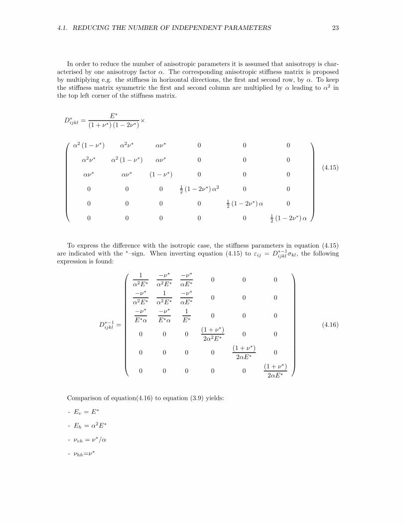
4.1. REDUCING THE NUMBER OF INDEPENDENT PARAMETERS 23
In order to reduce the number of anisotropic parameters it is assumed that anisotropy is char-acterised by one anisotropy factor α. The corresponding anisotropic stiffness matrix is proposedby multiplying e.g. the stiffness in horizontal directions, the first and second row, by α. To keepthe stiffness matrix symmetric the first and second column are multiplied by α leading to α2 inthe top left corner of the stiffness matrix.
D∗
ijkl =E∗
(1 + ν∗) (1 − 2ν∗)×
α2 (1 − ν∗) α2ν∗ αν∗ 0 0 0
α2ν∗ α2 (1 − ν∗) αν∗ 0 0 0
αν∗ αν∗ (1 − ν∗) 0 0 0
0 0 0 12 (1 − 2ν∗)α2 0 0
0 0 0 0 12 (1 − 2ν∗)α 0
0 0 0 0 0 12 (1 − 2ν∗)α
(4.15)
To express the difference with the isotropic case, the stiffness parameters in equation (4.15)are indicated with the ∗–sign. When inverting equation (4.15) to εij = D∗−1
ijkl σkl, the followingexpression is found:
D∗−1ijkl =
1
α2E∗
−ν∗α2E∗
−ν∗αE∗
0 0 0
−ν∗α2E∗
1
α2E∗
−ν∗αE∗
0 0 0
−ν∗E∗α
−ν∗E∗α
1
E∗0 0 0
0 0 0(1 + ν∗)
2α2E∗0 0
0 0 0 0(1 + ν∗)
2αE∗0
0 0 0 0 0(1 + ν∗)
2αE∗
(4.16)
Comparison of equation(4.16) to equation (3.9) yields:
- Ev = E∗
- Eh = α2E∗
- νvh = ν∗/α
- νhh=ν∗

24 CHAPTER 4. PARAMETER ASSESSMENT
- Gvh = αE∗/2 (1 + ν∗)
- Ghh = α2E∗/2 (1 + ν∗)
So a physical meaning of the anisotropy factor α can be seen as α =√Eh/Ev. For α = 1
equation (4.16) represents isotropic behaviour. The assumption that one anisotropy factor can beused to describe cross–anisotropy has limiting consequences. The ratio’s of the different stiffnessparameters are no longer independent;
√Eh/Ev = νhh/νvh = Ghh/Gvh. The comparison between
the equations (4.16) and (3.9) can be summarised by:
α =√Eh/Ev
α = νhh/νvh
α = Ghh/Gvh
(4.17)
Atkinson, Richardson & Stallebrass [4] use a more general form of equation (4.13):
δe
δεq
=
1
K ′
1
Jpq1
Jqp
1
3G′
δp′
δq
(4.18)
The subscripts pq and qp have been used, following Hird & Pierpoint [36]. Due to the distinctionbetween Jpq and Jqp anisotropy different from cross–anisotropy can also be modelled. For cross–anisotropy, which is assumed here, follows Jpq = Jqp = J ′. Atkinson, Richardson & Stallebrass[4] consider the parameters K ′, J ′ and G′ as tangent moduli. The use of tangent moduli allowsequation (4.18) to be used for non–linear elastic behaviour. Then values for K ′, J ′ and G′ arestress dependent. The δ–sign is used in equation (4.18) indicating that increments of stress andstrain are considered. The parameters K ′, G′ and J ′ are different from K∗, G∗ and J . Comparisonof (4.18) and (4.13) yields, [54]:
G∗ =G′J ′2
J ′2 − 3K ′G′(4.19)
K∗ =K ′J ′2
J ′2 − 3K ′G′(4.20)
J =−3G′K ′J ′
J ′2 − 3K ′G′(4.21)
and
G′ =3G∗K∗ − J2
3K∗(4.22)
K ′ =3G∗K∗ − J2
3G∗(4.23)
J ′ =−(3G∗K∗ − J2
)
J(4.24)
Appendix C shows that K ′, G′ and J ′ can be expressed in the traditional stiffness parameters,assuming the axis of symmetry in axial direction is found:
G′ =3
4 [(1 + 2νvh) /Ev + (1 − νhh) /2Eh](4.25)
K ′ =1
[(1 − 4νvh) /Ev + 2 (1 − νhh) /Eh](4.26)
J ′ =3
2 [(1 − νvh) /Ev − (1 − νhh) /Eh](4.27)

4.2. REPORTED MEASUREMENTS 25
In this three parameter description the restriction that one factor, α, controls the ratio ofdifferent parameters is not required. The K ′, J ′ and G′ model therefore represents more generalconditions than the α, E∗ and ν∗ model.
Lings, Pennington & Nash [54] use equation (4.1). It should be noted that the matrix inequation (4.1) is no longer symmetric. Each component can be derived from standard triaxialtests. However since the parameters νhh and Eh are not expressed independently, the individualvalues for νhh and Eh cannot be found. For this reason a parameter Fh is introduced by:
Fh =Eh
1 − νhh(4.28)
Lings, Pennington & Nash, [54], show that the parameters K ′, J ′ and G′ can be expressed intoEv, Fh and νvh, according to:
G′ =3EvFh
4Fh + 8νvhFh + 2Ev(4.29)
K ′ =EvFh
Fh − 4νvhFh + 2Ev(4.30)
J ′ =3EvFh
2Fh − 2νvhFh − 2Ev(4.31)
Rewriting gives:
Ev =9G′K ′J ′
6G′K ′ +G′J ′ + 3K ′J ′(4.32)
νvh = −1
2
3G′K ′ + 2G′J ′ − 3K ′J ′
6G′K ′ +G′J ′ + 3K ′J ′(4.33)
Fh =−18G′K ′J ′
12G′K ′ − 4G′J ′ − 3K ′J ′(4.34)
4.2 Reported measurements
....................................................................................................................................................................................................................................................................................................................................................................................................................................................... ...................
.....
.....
.....
.....
.....
.....
.....
.....
.....
.....
.....
.....
.....
.....
.....
.....
.....
.....
.....
.....
.....
.....
.....
.....
.....
.....
.....
.....
.....
.....
.....
.....
.....
.....
.....
.....
.....
.....
.....
.....
.....
.....
.....
.....
.....
.....
.....
.....
.....
.....
.....
.....
.....
.....
.....
.....
........................
...................
...................................................................................................................................................................................................................................................................................................................................................................................................................................................................................................................................................................................................................................................................................
.....
.....
...
.....
.....
...
.....
.....
...
.....
.....
...
.....
.....
...
.....
.....
...
.....
.....
...
.....
.....
...
.....
.....
.....
.....
...
.....
.....
...
.....
.....
...
.....
.....
...
.....
.....
...
.....
.....
...
.....
.....
...
.....
.....
...
.....
.....
...
.....
.....
I II III
log ε
E0
G0
E or G
ε0
verysmallstrain
smallstrain large strain
Figure 4.1: Typical stiffness–strain relation-ship, after [5]
Section 4.1 presents four three-parameter de-scriptions of cross–anisotropy given in the pa-rameters E∗, ν∗, α or K∗, G∗, J or K ′, G′,J ′ and Ev, νvh, Fh. Measurements of theseparameters presented in literature are limited.Most of the reported measurements concernstiff clay and sand. Measurements on peat werenot found. Using equations (4.19) to (4.21),(4.22) to (4.24), (4.29) to (4.31) and (4.32) to(4.34) the parameters measured for one modelcan be expressed into the parameters for theother models.
Before discussing reported measurementsthe strain dependency of stiffness parametersshould be noted. Figure 4.1 shows a typicalstiffness–strain relationship for soil, accordingto Atkinson [5]. Three regions can be distin-guished. In the first region, for very smallstrain, the stiffness is relatively large and strain independent. In the second region the stiffness de-creases and is clearly non–linear. However in the second region the behaviour can still be describedby equivalent elastic tangent moduli. In the third region the plastic deformation is considerable

26 CHAPTER 4. PARAMETER ASSESSMENT
and stiffness is strongly reduced. Jardine [39] describes the application of this phenomenon tomodelling soil behaviour. In a p′–q diagram the corresponding stress condition can be depicted.Even for largely over–consolidated conditions only a small zone around the actual stress conditionis found in which soil behaviour is truly linear elastic. This zone is referred to as zone I. Beyondthis zone a zone II is defined in which soil behaviour can be described as non–linear elastic. Aftera loading–unloading cycle within zone II the remaining deformation is negligible. However thestress–strain curve shows a hysteresis. Between zone II and some bounding surface lays zone III inwhich loading–unloading cycles lead to unrecoverable deformation and an increasing load reducesthe stiffness until failure is reached.
............................................................................................................................................................................................................................................................................................................................................................................................................................................................................................................
.....
.....
.....
.....
.....
.....
.....
.....
.....
.....
.....
.....
.....
.....
.....
.....
.....
.....
.....
.....
.....
.....
.....
.....
.....
.....
.....
.....
.....
.....
.....
.....
.....
.....
.....
.....
.....
.....
.....
.....
.....
.....
.....
.....
.....
.....
.....
.....
.......................
...................
..................................................................... ...................
..........................................................................................
...................
.....
.....
.....
.....
.....
.....
.....
.....
.....
........................
...................
.....................................................................
................... .....................................................................
.....
.....
.....
....
.................................................................................................................... ................
...
•
.............................
............................
.............................
............................
.............................
...............
A B
CD
E
F p′
q
θ
zone III
zone II
zone I
.........
....................................................................
..........................
..................................
........................
.......... ........ .......................... ........ ..................................
.....
..............................................................................................................................................................................................................................................
.....
............................................................
...............................
.......................... .................................................................
..........................................................................................................................................................................
.......................... ........ ..........................
.......................... ........ ..........................
..........................................................................................................................................................................
..........................
........
ABACADAEAF
> 0> 0
0< 0
0
0> 0> 0
0< 0
δp′ δq
Figure 4.2: Different stress path directions for deriving stiffness parameters
The boundary for zone I is reached for very small strain, 10−5 ([54], [38]) or even smallerfor some clays [39]. This implies that for some soil types true linear–elastic behaviour is beyondmeasurement accuracy. The non–linearity in zone II is explained by small plastic deformations atmicro–level where yielding occurs at the contact points of the solid particles. The boundary forzone II is found for strain of an order of magnitude of 10−4 to 4 × 10⁻⁴, [39].
The strain dependency of stiffness parameters has several consequences. Two are discussed infurther detail. First, Jardine [39] shows that the boundary of zone I and II is not symmetricalaround the considered stress condition. The shape of zone II depends on the stress history anddistance to the yield surface. Within zone I and II soil behaviour might be anisotropic, thoughwhen elastic parameters are derived by stress paths in different directions around some stresscondition an apparent anisotropy might be found due to an irregular shape of zone II. This is alsofound by Atkinson et al. [4] and Lings et al. [54]. Figure 4.2 shows different stress paths whichcan be followed to derive stiffness parameters. If a triaxial sample is brought to stress conditionA shown by figure 4.2, different stiffness parameters can be derived by applying stress paths likeAB, AC, AD, AE or AF. The angle between the stress path before consolidation and applied stresspath is indicated by θ in figure 4.2. Atkinson et al. [4] and Lings et al. [54] show that stiffnessparameters are θ–dependent.
The second consequence of the strain dependency of stiffness parameters is that comparisonof stiffness parameters is only valid when measured at the same strain level. Yimsiri & Soga [82]report an overview of measurements on the full set of five cross–anisotropic parameters. Table4.2 shows a summary. The reported parameters are derived from triaxial tests in combination tohorizontal and vertical shear wave measurements. Shear wave measurements involve very smalldisplacements. The parameters found by shear wave measurements can be considered as initial,zone I, values. Due to the measurement accuracy a reliable measurement for stiffness parametersby conventional axial or radial deformation measurement techniques are usually only found for zone

4.2
.R
EP
ORT
ED
ME
ASU
RE
ME
NT
S27
Table 4.1: Cross–anisotropic elastic parameters for clay
material ref. stress G∗ K∗ J α E∗ ν∗ νvh Fhcondition G′ K ′ J ′ Ev
Winnipeg Clay [34] in situc 8.5a ×σ′vc 14.5a ×σ′
vc -5.5a ×σ′vc 1.33a 18.5e ×σ′
vc 0.22a 0.17e 36.7e ×σ′vc
7.8d ×σ′vc 13.3d ×σ′
vc 61.7d ×σ′vc
Gault Clay [54] in situ 663d ×p′0 613d ×p′0 -715d ×p′0 1.95 550f ×p′0 0 0a 2100a ×p′0K0 ≈ 2 385a ×p′0 356a ×p′0 990a ×p′0 550a ×p′0
London Clay [4] isotropic - - -p′0 = 200 kPa 37a [MPa] 60a [MPa]OCR = 2
Oxford Clay [36] isotropic 173d [MPa] 259d [MPa] -333d [MPa] 1.7 43e [MPa] - 0.03e 1030e [MPa][37] p′0 = 150 45a [MPa] 30a [MPa] 125ab [MPa]
a = measured values bJ ′ = 0.5(J ′pq + J ′
qp)c = K0 not given in [34], φ′ = 17.5◦K0 ≈ 1 − sinφ′ = 0.7
d = eq. (4.19) to (4.24) e = eq.(4.32) to (4.34) f = eq. (4.17)
Table 4.2: Cross–anisotropic elastic parameters according to [82]stress α α α
Material ref. condition Ev Eh Gvh Ghh νhh νvh νhv√Eh/Ev Ghh/Gvh νhv/νhh
[MPa] [MPa] [MPa] [MPa]Dry Mortar sand [67] isotropic 242.9 304.0 108.1 132.8 0.145 0.201 0.251 1.12 1.23 1.73
p′= 85 kPaK0= 1.7 236.8 320.2 110.6 135.3 0.183 0.066 0.091 1.16 1.22 0.50σ′v = 50 kPa
Dry Ticino sand [11] K0 = 0.5 386.6 306.2 135.4 127.8 0.198 0.143 0.133 0.89 0.94 0.67σ′v = 300 kPaK0 = 1.5 245.9 372.5 123.9 156.0 0.194 0.092 0.154 1.23 1.26 0.79σ′v = 150 kPaK0 = 2 188.5 353.8 104.4 150.9 0.172 0.141 0.264 1.37 1.45 1.53σ′v = 100 kPa
isotropic 287.9 349.4 125.2 149.1 0.172 0.177 0.215 1.10 1.19 1.25p′ = 200 kPa
Saturated Ham [50] K0 = 0.45 520 280 154 130 0.07 0.35 0.19 0.73 0.84 2.71River sand σ′
v = 316 kPaGault Clay [54] in situ stress 550 2186 507 1140 -0.04 0 0 2.0 2.25 0
K0 ≈ 2 ×p′0 ×p′0 ×p′0 ×p′0
28 CHAPTER 4. PARAMETER ASSESSMENT
II and III. This difference should be realised when comparing the results of different measurementtechniques.
So it is therefore concluded that the actual value for a stiffness parameter depends on loadhistory and strain level at which the parameter is measured. In literature this is not alwaysacknowledged. When gathering measurement data from literature stress history is not alwayspresented or measurements of strain gauges are mixed with shear wave measurements. Keepingthese remarks in mind, table 4.1 and 4.2 give the possibility to check some of the assumptionsmade for the three-parameter models. Table 4.2 shows the values for α found from the measuredcross–anisotropic parameters. Except for Ham River sand and Gault Clay, table 4.2 shows that thevalues for the three α–definitions, as shown by equation (4.17), are of the same order of magnitude.Due to the low value for νhh respectively νhv the definition of α = νhv/νhh for Ham River sandand Gault Clay does not correspond to the values for the other definitions. The assumptionα =
√Eh/Ev = νhh/νvh = Ghh/Gvh seems not to hold for small values for νhv and νhh.
Another important assumption is the symmetry of matrix in equation (4.18), J ′pq = J ′
qp = J ′.For Gault Clay and Oxford Clay separate measurements of J ′
pq and J ′qp are presented in [54] and
[37] respectively. For Oxford Clay a distinction has been made between loading and unloadingconditions, (δq > 0, δq < 0). For unloading conditions it is found that Jpq ≈ Jqp ≈ J ′ ≈ 70 kPa.For loading conditions however Jpq reaches 180 kPa for small strain, Jqp corresponds to the valuesfound for unloading. Larger strain gives Jpq ≈ Jqp ≈ J ′. The value for J ′ presented in table 4.1follows from J ′ = 0.5 (Jpq +Jqp). The presented value for α is calculated using this average value.It should be noted that J ′ → ∞ indicates isotropic conditions. Small J ′–values indicate stronganisotropy, J ′ = 70 kPa corresponds to α = 4.89.
For Gault Clay [54] values for Jpq and Jqp are derived in tests with constant p′ and constant q.For small strain energy it is found that Jpq ≈ Jqp ≈ J ′ = 800–1000 kPa at small strain level. Thedifferences in the measured J ′-value are explained by the difficulty in measuring J ′ at small strainlevels.
4.3 Undrained tests
4.3.1 Initial pore pressure
An important feature in undrained loading is the development of excess pore pressure under con-stant volume deformation. In engineering practice undrained behaviour plays an important rolewhen dealing with soft, low permeable soil types like clay and peat. Initially after loading thesesoil types behave undrained. Pore pressure will then decrease and deformations emerge when con-solidation proceeds. Loading can be considered as instantaneous, since the time needed for loadapplication is considerably smaller than the hydrodynamic period. The amount of pore pressuredirectly after loading is referred to as initial pore pressure. In the laboratory undrained triaxialtesting can be used to reproduce these initial conditions. In the following expressions are de-rived for initial pore pressure reaction for axial symmetric isotropic and cross–anisotropic materialbehaviour. The expressions show that the initial pore pressure is strongly influenced by anisotropy.
The isotropic caseDe Josselin de Jong [41] presents a mathematical formulation for calculating the initial porepressure when loading a soil sample for the isotropic case. Starting point is the initial volumechange e0 which equals the initial change in pore water volume. So, with K for soil bulk modulusand Kw for pore water stiffness the following is found:
e0 =p′
K= σw0
n
Kw
(4.35)

4.3. UNDRAINED TESTS 29
followed by:
p′ = Ke0 σw0 =Kw
ne0
p = p′ + σw0 = Ke0 +Kw
ne0 =
(nK +Kw
n
)e0
e0 = p
(n
nK +Kw
)= σw0
n
Kw
σw0= Bp; B =
1
nK
Kw
+ 1
(4.36)
The parameter B in equation (4.36) represents the Skempton B–factor [65]. For fully saturatedsoil Kw ≫ K and B = 1. Equation (4.36) shows that the initial pore pressure equals the isotropicstress increase for an isotropic, fully saturated, soil type. In standard triaxial testing with σr = 0and p = σa/3 is found:
σw0 =σa3
(4.37)
The cross–anisotropic caseThe relation between the anisotropic stiffness parameters and the initial pore pressures is givenby equation (4.18)
e0 =p′
K ′+
q
J ′= σw0
n
Kw
(4.38)
reformulation gives:
K ′J ′e0 = J ′ (p− σw0) +K ′q, σw0 =Kw
ne0
e0 =
(n
nK ′ +Kw
)(p+
K ′
J ′q
)=
n
Kw
σw0 (4.39)
σw0 = B
(p+
K ′
J ′q
), B =
1
nK ′
Kw
+ 1
(4.40)
The influence of anisotropy on the Skempton B–factor is given by the replacement of K by K ′.For isotropic conditions K ′ → K and K ′/J ′ → 0 is found that equation (4.40) reduces to (4.36).Equation (4.40) shows the influence of anisotropy on σw0. For fully saturated soil in standardtriaxial testing, σr = 0, p = 1/3σa and q = σa is found:
σw0 =
(1
3+K ′
J ′
)σa (4.41)
It should be noted that expression (4.41) presents the initial excess pore pressure for initial,undrained, conditions in terms of drained stiffness parameters. Another expression for the initial

30 CHAPTER 4. PARAMETER ASSESSMENT
pore pressure for a fully saturated soil under axial symmetric conditions is presented by Chowdhury[21]:
σw0 =(1 − νhh − ηνvh) 2σr + (η − 2ηνvh)σa
η − 4νvhη + 2 − 2νhh, η =
EhEv
(4.42)
Application of the equations (4.26) and (4.27) to equation (4.41) shows equations (4.42) and (4.41)to be equivalent.
4.3.2 Drained and undrained stiffness parameters
In engineering practice undrained analyses are often conducted using a total stress analysis in whichundrained behaviour is modelled as a constant volume deformation. For isotropic conditions this isachieved by adjusting the stiffness parameters such that the bulk modulus reaches an infinite valuewhile the shear modulus remains unaltered. Drained and undrained stiffness parameters shouldnot be mixed. To distinguish undrained parameters the superscript u is used.
Equation (4.35) shows for partly saturated soil, B < 1, that undrained deformations do notcorrespond to constant volume deformations. Chapter 2 states that partly saturated soil can bemodelled by the pore fluid stiffness for Sr > 0.85. Elaborating equation (4.35) for this condition incombination to Hooke’s law for isotropic conditions gives for the undrained stiffness parameters,[15]:
Eu =3E
3 −B (1 − 2ν); νu =
3ν +B (1 − 2ν)
3 −B (1 − 2ν)(4.43)
Section 3.2 discusses the bounding values for the cross anisotropic stiffness parameters. This isvisualised by figure 3.4, which is repeated by figure 4.3.
Section 3.2 explains that each valid combination of stiffness parameters falls in or is on the”ship-bow” like shape presented by figure 4.3. Section 3.2 explains that the line AB represents thecombination of stiffness parameters which give constant volume deformation. For soil completelysaturated by an incompressible fluid these parameters can be regarded as the cross–anisotropicundrained stiffness parameters. It is remarkable that for undrained behaviour the ratio (Eh/Ev)
u
is maximised to 4. As shown by figure 4.3 for Eh/Ev > 4 no constant volume deformation ispossible within the range of valid νhh values. This illustrates that the level of anisotropy is lessdistinct for undrained conditions than for drained conditions.
............................................................................................................................................................................................................................................................................ ...................
.....
.....
.....
.....
.....
.....
.....
.....
.....
.....
.....
.....
.....
.....
.....
.....
.....
.....
.....
.....
.....
.....
.....
.....
.....
.....
.....
.....
.....
.....
.....
.....
.....
.....
.....
.....
.....
.....
.....
.....
.....
.....
.....
.....
.....
.....
.....
.....
.....
.....
.....
.....
.....
.....
.....
.....
.....
.....
.....
.....
.....
.....
.....
.....
.....
.....
.....
.....
.....
.....
.....
....................
...................
..................................................................................................................................................................................................................................................................
...................
.........................................................................................................................................................................................................................................................................................................................................................
................................................................................................................................................................................................................................................................................................................................................
......................................................................................................................................................................................................................................................................................................................................
..........................................................................................................................................................................................................................................................................................................................
.....
......
......
.....
......
......
.....
......
......
......
.....
......
......
.....
......
.....
.....
.....
.....
.....
.....
.....
.....
.....
.....
.....
.....
.....
......
.....
.....
.....
.....
.....
.....
.....
.....
.....
.....
.....
.....
.....
......
.....
.....
.....
.....
.....
.....
.....
.....
.....
.....
.....
.....
.....
......
.....
.
............................................
.............................
.......................................
...............................................................................................................
.......................................................
................................
.............................
............................
............................
...........................
...........................
...................
................................................................................
...................................
................................
...............................
.............................
.............................
...........................
.........................
..................................................................................................
.......................................
...................................
.................................
..............................
...............................
.............................
......................................................................
...............................................
.......................................
...................................
..................................
................................
...............................
...............................
...........
.....................................................................................................................
.....
.....
.....
.....
.....
.....
.....
.....
.....
.....
.....
.....
.....
.....
.....
.....
.....
.....
.....
.....
.....
.....
.....
.....
.....
.....
.....
.....
.....
.....
.....
.....
.....
.....
.....
.....
.....
.....
.....
.....
.....
.....
.....
.....
.....
.....
.....
.....
.....
.....
.....
.....
.....
.....
.....
.....
.....
.....
.....
.....
.....
.....
.....
.....
.....
.....
....................
.............
...........
...........
....................................................................................................................................
......................
...........
...........
.............................................................................................................................................
......................
...........
...............................................................................................................................................
...........
.................................................................................................................................................................
..................................................................
.....
.........................................................
..................................................
.....
.......................................
........................................................
................................................................................
................................................................................................................
...........................................................................................................................................
...............................................................................................................................................................
0.5
1
2
3
4
EhEv
-1-0.5
00.5
1
νhv
EhEv
νhh
............................................................................................................................................................................................................................................................................ ...................
.....
.....
.....
.....
.....
.....
.....
.....
.....
.....
.....
.....
.....
.....
.....
.....
.....
.....
.....
.....
.....
.....
.....
.....
.....
.....
.....
.....
......................
...................
..................................................................................................................................................................................................................................................................
...................
.........................................................................................................................................................................................................................................................................................................................................................
................................................................................................................................................................................................................................................................................................................................................
......................................................................................................................................................................................................................................................................................................................................
..........................................................................................................................................................................................................................................................................................................................
.....
......
......
.....
......
......
.....
......
......
......
.....
......
......
.....
......
.....
.....
.....
.....
.....
.....
.....
.....
.....
.....
.....
.....
.....
......
.....
.....
.....
.....
.....
.....
.....
.....
.....
.....
.....
.....
.....
......
.....
.....
.....
.....
.....
.....
.....
.....
.....
.....
.....
.....
.....
......
.....
.
.......................................................
................................
.............................
............................
............................
...........................
...........................
...................
.....
...............................................................................................................................................................................................................................................................
......................................................................................................................................................................................................................................................................................................................................................................................................................................................................................................................................................................................................................................................................................................................................................................................................................................................................................................................................................
......................................................
....................
.............
...........
...........
....................................................................................................................................
........................................................
................................................................................................................
...........................................................................................................................................
...............................................................................................................................................................
Eh/Ev = 1
νhv
EhEv
νhh
• A
•B
•C
•D
Figure 4.3: Bounding values for anisotropic linear elastic parameters after [61]

4.3. UNDRAINED TESTS 31
For isotropic conditions there is a unique relation between the drained and undrained stiffnessparameters as shown by equation (4.43). Cross–anisotropy however does not exhibit such an uniquerelation. When B = 1 the undrained behaviour of a soil type with any combination of drainedparameters is represented by some unique point on the line AB in figure 4.3. So any combination ofdrained parameters can be uniquely mapped to undrained parameters, however some combinationof undrained parameters represent a large number of valid combinations of drained parameters.
Elaborating equation (4.38) and (3.9) expresses the undrained stiffness parameters into drainedparameters as shown by appendix D. The result is:
Euv =Ev [(1 − 4νvh)Eh + 2 (1 − νhh)Ev]
Eh
[(1 − 4νvh) −B (1 − 2νvh)
2]
+ 2 (1 − νhh)Ev
Euh =EvEhd
Evd−B[E2v (1 − νhh)
2 − 2EvEhνvh (1 − νhh) + ν2vhE
2h
]
νuvh =νvhEh [(1 − 4νvh) −B (1 − 2νvh)] + (1 − νhh)Ev [2νvh +B (1 − 2νvh)]
Eh
[(1 − 4νvh) −B (1 − 2νvh)
2]
+ 2 (1 − νhh)Ev
νuhh =νhhEvd+B
[E2v (1 − νhh)
2+ E2
hν2vh − 2EhEvνvh (1 − νh)
]
Evd+B[2EvEhνvh (1 − νhh) − E2
v (1 − νhh)2 − ν2
vhE2h
]
with
d = (1 − 4νvh)Eh + 2 (1 − νhh)Ev
(4.44)
Note that the shear modulus remains unaffected so, Guhh = Ghh and Guvh = Gvh. For Euv andEuh the expressions for their reciprocal values are also given in appendix D since these expressionsnicely show the influence of the B–factor. For completely saturated soil, B = 1, is found, a.o.Lings in [55]:
νuvh =1
2νuhh = 1 − 1
2
EuhEuv
For B = 1 the number of independent cross–anisotropic parameters is reduced from 5 to 3, Euv ,Euh and Guvh. This corresponds to figure 4.3 which depicts undrained deformation by a single line,the line AB.
4.3.3 The undrained effective stress path
.................................................................................................................................................................................................................................................................................................................................. ...................
.....
.....
.....
.....
.....
.....
.....
.....
.....
.....
.....
.....
.....
.....
.....
.....
.....
.....
.....
.....
.....
.....
.....
.....
.....
.....
.....
.....
.....
.....
.....
.....
.....
.....
.....
.....
.....
.....
.....
.....
.....
.....
.....
.....
.....
.....
.....
.....
.....
.....
.....
.....
.....
.....
.....
.....
.....
.....
.....
.....
......................
...................
.....
.....
.....
.....
.....
.....
.....
.....
.....
.....
.....
.....
.....
.....
.....
.....
.....
.....
.....
.....
.....
.....
.....
.....
.....
.....
.....
.....
.....
.....
.....
.....
.....
.....
.....
.....
....
................................................................................................................................................................................................
............................................
..................
.....
.....
.....
.....
.....
.....
.....
.....
.....
.....
.....
.....
.....
...
.............................................................................................................................................
.....................................................................................................................................................................
p′
q
p
σw
13σb
K′
J′σb
1
3
TSP
ESP
ψ
1..........................................................................................................................
....
....
....
....
....
....
....
....
....
....
....
....
....
....
....
....
....
....
....
....
....
....
....
....
....
....
....
....
....
....
..
Figure 4.4: Typical stress paths for a linearelastic material
Figure 4.4 shows a typical Total Stress Path (TSP)and an Effective Stress Path (ESP) for undrainedelastic conditions. In figure 4.4 σb represents theaxial load increment applied at the top of thesample. The intercept between both paths cor-responds to the pore pressure development insidethe sample. For a standard undrained axial com-pression test, by definition of p and q, the TSPhas a slope of 1:3. In an undrained test an incre-ment in vertical load gives a pore pressure reactionas presented in equation (4.40). The slope of theESP, ψ in fig 4.4, is dictated by the ratio K ′/J ′,ψ = −J ′/K ′ . For an isotropic elastic material,K ′/J ′ = 0, a vertical ESP is found. For K ′/J ′ >0, the pore pressure development exceeds the in-crease in p leading to a reduction in p′. A back-
32 CHAPTER 4. PARAMETER ASSESSMENT
wardly tilting ESP is found. If K ′/J ′ < 0, an increase in p′ is found producing a forwardly tiltingESP.
The ratio K ′/J ′ can be expressed in Eh, Ev, νhh and νvh using the equations given in appendixC. If the axial direction of the sample corresponds to the axis of symmetry, referred to as thevertical direction, is found:
K ′
J ′=
2
3
[(1 − νvh) η − (1 − νhh)
(1 − 4νvh) η + 2 (1 − νhh)
], η =
EhEv
(4.45)
If the axis of symmetry is aligned in one of the radial directions a different expression for J ′ isfound as shown in appendix C. This condition is found when e.g. a sample is retrieved horizontallyfrom a cross–anisotropic soil layer, which has a vertical axis of symmetry. For K ′/J ′ it is thenfound:
K ′
J ′=
−1
3
[(1 − νvh) η − (1 − νhh)
(1 − 4νvh) η + 2 (1 − νhh)
], η =
EhEv
(4.46)
For isotropic conditions both equations (4.45) and (4.46) give K ′/J ′ = 0. However for all othercombinations of stiffness parameters equations (4.45) and (4.46) lead to K ′/J ′ values with anopposite sign. If in an undrained triaxial test on a vertically retrieved sample a backward tiltingESP is found then an undrained triaxial test on a horizontally retrieved sample from the same soillayer will show a forward tilting ESP and vice versa. The absolute value of the ESP slopes foundfrom a horizontally retrieved sample is smaller than those from a vertically retrieved sample.
It is remarkable that equations (4.45) and (4.46) show singular points for valid combinationsfor Eh, Ev, νvh and νhh. These values are found when:
(1 − 4νvh)EhEv
+ 2 (1 − νhh) = 0
This condition corresponds toK ′ = ∞, according to equation (4.26) or (3.17), it represents constantvolume deformation.
For small values for νvh < 0.25 and νhh < 0.25 singularity of equations (4.45) and (4.46) doesnot occur. Then the maximum and minimum values for K ′/J ′ are dominated by the ratio Eh/Ev.According to equation (4.45) for Eh/Ev = 0 the lower boundary is found; K ′/J ′ = -1/3. Equation(4.41) shows that, for this lower boundary, no excess pore pressure is created. With K ′/J ′ = -1/3the slope of ESP is -1:3 and ESP equals TSP. The upper boundary is found if Eh/Ev → ∞ thenK ′/J ′ = 2/3. The slope of ESP becomes 2:3. Equation (4.41) shows that for K ′/J ′ = 2/3 it isfound that σw0 = σa.
Graham & Houlsby in [34] give the following expression for the ESP in G∗, J and α, ν∗:
q
p′=
3G∗
J=
3(2 − 2ν∗ − 4αν∗ + α2
)
2 (1 − ν∗ + αν∗ − α2)(4.47)
Application of the equations presented in appendix C shows that equation (4.47) corresponds toequation (4.45).
Measurements of the angle of ESP in relation to stiffness parameters are presented by Wesley[81] for Mucking Flat clay and by Graham & Houlsby for Winnipeg Clay [34]. For Winnipeg Claythe slope of ESP ranges from -15.8 to -4.45, with an average value of -6.8. This corresponds toK ′/J ′ = 0.15. Table 4.1 presents the values for K ′ and J ′, showing K ′/J ′ = 0.22.
The influence of anisotropy on the ESP is extensively studied by Wesley [81] for Mucking Flatclay from the bedding of the river Thames. For this type of clay a clear difference in loadingand unloading stiffness is found. A triaxial sample loaded undrained in axial direction faces areduction in radial effective stress due to the pore pressure reaction. So axial loading leads toradial unloading. The K ′/J ′ value then depends not only on the isotropy in stiffness parametersbut also on loading conditions. As shown by Parry & Wroth [62] a vertically retrieved sample

4.3. UNDRAINED TESTS 33
of Mucking Flat clay axially loaded shows a vertical ESP corresponding to K ′/J ′ = 0 and doesnot seem to behave anisotropically. A vertical sample loaded into extension gives an angle of ESPequal to 1:-2.18 leading to K ′/J ′ = 0.46. For an horizontally retrieved sample the opposite isfound. When loaded into extension a vertical ESP is found, while loaded in compression the angleof ESP is 1:-2.4 or K ′/J ′ = 0.4.
Lings [55] gives a simplification of figure 3.4 expressed in Fh, Ev and νvh. With Fh = Eh/(1−νhh) applied to equation (3.14) the ”ship-bow”-like structure is now reduced to a parabola as shownby figure 4.5. All valid combinations of Fh, Ev and νvh are located inside or on the parabola.Uncoupled and incompressible behaviour are reduced to lines in this graph. The intersection ofthose lines gives the point of undrained material behaviour. This means that there is only onecombination of Fuh , Euv and νuvh. Rewriting equation (4.45) in terms of Fh, Ev and νvh gives:
K ′
J ′=
2
3
(1 − νvh) −EvFh
(1 − 4νvh) +2EvFh
(4.48)
Equation (4.48) can be used to depict lines of equal K ′/J ′ values in figure 4.5. Each line runsthrough the undrained spot. Evidently the line for K ′/J ′ = 0 corresponds to the line representinguncoupled materials. Lines above the uncoupled line represent K ′/J ′ < 0, a forward tilting ESP,and the lines underneath represent K ′/J ′ > 0, a backward tilting ESP. Lings [55] shows thatmeasurements, reported in literature, plot on the right–hand side of the parabola, νvh > 0.
−1.00 −0.75 −0.50 −0.25 0.00 0.25 0.50 0.75 1.00
νvh
0.00
0.25
0.50
0.75
1.00
1.25
1.50
1.75
2.00
Ev/Fh
........................................................................................................................................................................................................................................................................................................................................................................................................................................................................................................................................................................................................................................................................................................
......................................
....................
..............................................................................................................................................................................................................................................................................................................................................................................................................................................................................................................................................................................................................................................
•
Bound on elastic parameters
Undrained point..................................................
...................................................
..................................................
...............................................
....................................................
....................................................
....................................................
....................................................
....................................................
....................................................
....................................................
....................................................
....................................................
....................................................
....................................................
..........................
K′/J ′ = 0 (uncoupled behaviour).......................... ............
.............. ............
.............. ...........
................................................................... ............
.............. ............
.............. ............
.................................................................. ............
.............. ............
.............. ...........
......................................... K′/J ′ = 0.3
................................................................................................................................................................................................................................................................................................................ K′/J ′ = 2/3
....................................................
....................................................
....................................................
....................................................
....................................................
....................................................
....................................................
....................................................
....................................................
.........
K′/J ′ = -0.1
.....
.....
.....
.....
.....
.
.....
.....
.....
.....
.....
.
.....
.....
.....
.....
.....
.
.....
.....
.....
.....
.....
.
.....
.....
.....
.....
.....
.
.....
.....
.....
.....
.....
.
.....
.....
.....
.....
.....
.
.....
.....
.....
.....
.....
.
.....
.....
.....
.....
.....
.
.....
.....
.....
.....
.....
.
.....
.....
.....
.....
.....
.
.....
.....
.....
.....
.....
.
.....
.....
.....
.....
.....
.
.....
.....
.....
.....
.....
.
.....
.....
.....
.....
.....
.
.....
.....
.....
.....
.....
.
.....
.....
K′/J ′ = -1/3
......................................................................................................................................................................................................................................................................................................................................................................... K′/J ′ = ∞ (incompressible)
Figure 4.5: Elastic limits, dashed lines present combinations of constant K ′/J ′, from [55]

34 CHAPTER 4. PARAMETER ASSESSMENT
Chapter 5
3D consolidation
5.1 Introduction
This chapter discusses the influence of anisotropy on the consolidation behaviour of soft soil. Basedon Hooke’s law for cross–anisotropy derived in chapter 3 the three–dimensional solution for theconsolidation problem for axial symmetric and plane strain conditions are given in the appendicesE to I.
This chapter first presents a short literature overview, in which the Mandel–Cryer effect isintroduced. Based on the mathematical analysis given in appendices E and F section 5.3 high-lights some aspects of the 3D consolidation for isotropic linear elastic material behaviour for axialsymmetric and plane strain conditions. Section 5.4 discusses the differences in consolidation forisotropic and cross–anisotropic linear elasticity. Once a solution for the consolidation problem isfound a large number of alternatives using slightly different boundary conditions are easily derived.Section 5.5 discusses some of these solutions.
5.2 Literature overview
The first who gave a solution for the consolidation problem is Terzaghi in [70], for 1D conditions.Rendulic [64] gives a solution for the consolidation equation based on radial dissipation of porewater. Carillo presented a method to combine both results [17]. By combining vertical and radialdissipation a semi three–dimensional description of the consolidation behaviour is found. In 1947Barron [10] presents a solution for consolidation around a vertical drain combining axial and radialpore pressure dissipation. Both, the solution of Barron and Carillo, are based on the followingassumptions:
- The soil skeleton behaves linear elastic
- The soil is fully saturated by an incompressible fluid
- The soil is homogeneous
- Permeability and stiffness remain constant during consolidation
- Pore water flow is described by Darcy’s law
- Deformations remain small
In 1941 Biot published the derivation for a complete three–dimensional description of con-solidation behaviour ([12], [13] and [14]). Although the Biot equations are also based on theassumptions given above, a remarkable difference is found between the Biot equations and the
35
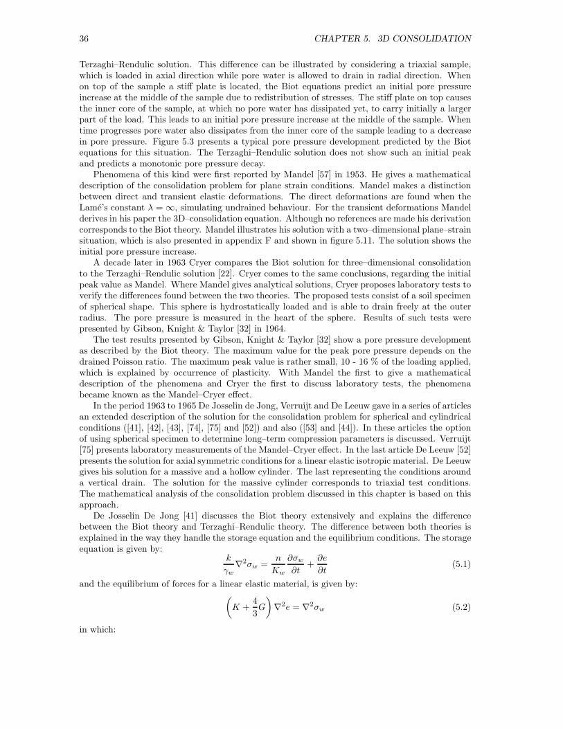
36 CHAPTER 5. 3D CONSOLIDATION
Terzaghi–Rendulic solution. This difference can be illustrated by considering a triaxial sample,which is loaded in axial direction while pore water is allowed to drain in radial direction. Whenon top of the sample a stiff plate is located, the Biot equations predict an initial pore pressureincrease at the middle of the sample due to redistribution of stresses. The stiff plate on top causesthe inner core of the sample, at which no pore water has dissipated yet, to carry initially a largerpart of the load. This leads to an initial pore pressure increase at the middle of the sample. Whentime progresses pore water also dissipates from the inner core of the sample leading to a decreasein pore pressure. Figure 5.3 presents a typical pore pressure development predicted by the Biotequations for this situation. The Terzaghi–Rendulic solution does not show such an initial peakand predicts a monotonic pore pressure decay.
Phenomena of this kind were first reported by Mandel [57] in 1953. He gives a mathematicaldescription of the consolidation problem for plane strain conditions. Mandel makes a distinctionbetween direct and transient elastic deformations. The direct deformations are found when theLame’s constant λ = ∞, simulating undrained behaviour. For the transient deformations Mandelderives in his paper the 3D–consolidation equation. Although no references are made his derivationcorresponds to the Biot theory. Mandel illustrates his solution with a two–dimensional plane–strainsituation, which is also presented in appendix F and shown in figure 5.11. The solution shows theinitial pore pressure increase.
A decade later in 1963 Cryer compares the Biot solution for three–dimensional consolidationto the Terzaghi–Rendulic solution [22]. Cryer comes to the same conclusions, regarding the initialpeak value as Mandel. Where Mandel gives analytical solutions, Cryer proposes laboratory tests toverify the differences found between the two theories. The proposed tests consist of a soil specimenof spherical shape. This sphere is hydrostatically loaded and is able to drain freely at the outerradius. The pore pressure is measured in the heart of the sphere. Results of such tests werepresented by Gibson, Knight & Taylor [32] in 1964.
The test results presented by Gibson, Knight & Taylor [32] show a pore pressure developmentas described by the Biot theory. The maximum value for the peak pore pressure depends on thedrained Poisson ratio. The maximum peak value is rather small, 10 - 16 % of the loading applied,which is explained by occurrence of plasticity. With Mandel the first to give a mathematicaldescription of the phenomena and Cryer the first to discuss laboratory tests, the phenomenabecame known as the Mandel–Cryer effect.
In the period 1963 to 1965 De Josselin de Jong, Verruijt and De Leeuw gave in a series of articlesan extended description of the solution for the consolidation problem for spherical and cylindricalconditions ([41], [42], [43], [74], [75] and [52]) and also ([53] and [44]). In these articles the optionof using spherical specimen to determine long–term compression parameters is discussed. Verruijt[75] presents laboratory measurements of the Mandel–Cryer effect. In the last article De Leeuw [52]presents the solution for axial symmetric conditions for a linear elastic isotropic material. De Leeuwgives his solution for a massive and a hollow cylinder. The last representing the conditions arounda vertical drain. The solution for the massive cylinder corresponds to triaxial test conditions.The mathematical analysis of the consolidation problem discussed in this chapter is based on thisapproach.
De Josselin De Jong [41] discusses the Biot theory extensively and explains the differencebetween the Biot theory and Terzaghi–Rendulic theory. The difference between both theories isexplained in the way they handle the storage equation and the equilibrium conditions. The storageequation is given by:
k
γw∇2σw =
n
Kw
∂σw∂t
+∂e
∂t(5.1)
and the equilibrium of forces for a linear elastic material, is given by:(K +
4
3G
)∇2e = ∇2σw (5.2)
in which:

5.2. LITERATURE OVERVIEW 37
K = compression modulus of soilG = shear moduluse = volumetric strainσw = pore pressureγw = volumetric weight of waterk = permeabilityKw = bulk modulus of pore watern = porosity∇2 = Laplace operator, ∇2 = ∂2/∂x2 + ∂2/∂y2 + ∂2/∂z2
Following De Josselin de Jong, a relation between e and σw can be found by twice integratingequation (5.2).
(K +
4
3G
)e = σw + f(x, y, z, t) (5.3)
In (5.3) the function f(x, y, z, t) should satisfy the condition ∇2f = 0. Eliminating e from equations(5.1) and (5.3) gives the consolidation equation:
k
γw∇2σw =
n
Kw
∂σw∂t
+1(
K +4
3G
)(∂σw∂t
+∂f (x, y, z, t)
∂t
)(5.4)
Terzaghi assumes a direct relation between σw and e leading to f = 0. In absence of ∂f/∂tequation (5.4) reduces to the well–known heat equation which has been studied extensively andmany solutions are available in literature. The presence of the function f(x, y, z, t) in the Biotequations makes the consolidation problem no longer analogous to the heat equation. It constitutesan essential difference between the Biot theory and Terzaghi solution.
De Josselin de Jong shows that in absence of rotations during deformation f(x, y, z, t) reducesto f(t), but not necessarily 0. An important exception is found for a one–dimensional geometryand loading conditions constant in time. Then it follows that the absolute value of f equals theapplied load. In equation 5.4 ∂f/∂t reduces to 0. For these conditions the Terzaghi solution equalsthe Biot theory.
In his paper on cylindrical consolidation, De Leeuw disregards the compressibility of the porewater in (5.1) and expresses the consolidation equation in terms of volumetric strain. Solving theconsolidation equation for e circumvents the need for a definition of f(x, y, z, t) in (5.2). Mandelapplied the same strategy in his paper [57] when deriving his solution for plane strain consolidation.
............................................................. ..........................................................................................................................................................................
............................................................. ...................................................................................................................................................................................................................................
............................................................. ..........................................................................................................................................................................
............................................................. ..........................................................................................................................................................................
..................................................................................................................................................................................................................................................
..................................................................................................................................................................................................................................................
.....
.....
.....
.....
.....
.....
.....
.....
.....
.....
.....
.....
.....
.....
.....
.....
.....
.....
.....
.....
.....
.....
.....
.....
.....
.....
.....
..
.....
.....
.....
.....
.....
.....
.....
.....
.....
.....
.....
.....
.....
.....
.....
.....
.....
.....
.....
.....
.....
.....
.....
.....
.....
.....
......
.....
......................
.....
.....
......................................................................................................................
...................
.............................................................. ...................
..............................................................
...................
........................................................................
...................
................
................
................
...........................................
.....
.....
.....
.....
.....
.....
.....
.....
......................
...................
Q
clay
sand
clay
sand.
.
.
.
.
.
.
.
.
.
.
.
.
.
.
.
.
.
.
.
.
.
.
.
.
.
.
.
.
.
.
.
.
.
.
.
.
.
.
.
.
.
.
.
.
.
.
.
.
.
.
.
.
.
.
.
.
.
.
.
.
.
.
.
.
.
.
.
.
.
.
.
.
.
.
.
.
.
.
.
.
.
.
.
.
.
.
.
.
.
.
.
.
.
.
.
.
.
.
.
.
.
.
.
.
.
.
.
.
.
.
.
.
.
.
.
.
.
.
.
.
.
.
.
.
.
.
.
.
.
.
.
.
.
.
.
.
......................
......................
......................
......................
......................
......................
......................
......................
......................
......................
......................
......................
......................
......................
......................
......................
......................
......................
......................
......................
......................
......................
......................
......................
......................
......................
......................
......................
......................
......................
......................
Figure 5.1: Conditions for the Noordbergumeffect
De Leeuw [53] presents a three–dimensional so-lution for the consolidation problem around a ver-tical drain based on the Biot theory. In this paperDe Leeuw shows that the function f becomes afunction of the time–derivative of the boundaryconditions. The boundary conditions are given interms of loading on top, pore pressure in the drainand radial deformation of inner and outer radius ofthe cylinder. For most engineering purposes theseboundary conditions are constant. So, in engineer-ing practice, for vertical drains, there is no differ-ence between the Terzaghi and the Biot theory.
In 1969 Verruijt [76] describes the Noordber-gum effect. The Noordbergum effect is found in a
double layered artesian aquifer, see figure 5.1. When water is extracted from the upper aquifersome water will leak from the lower aquifer through the separating clay layer to the upper aquifer.This leads to consolidation effects in the lower aquifer. Pore pressure measurements in the lower
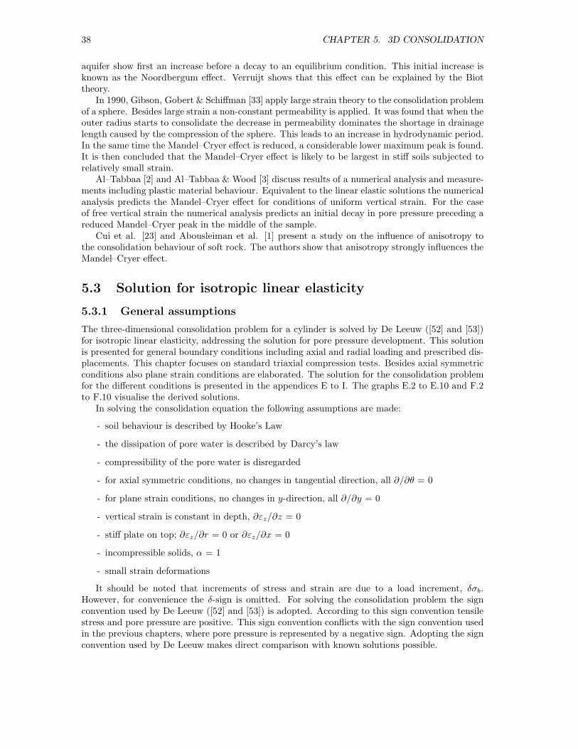
38 CHAPTER 5. 3D CONSOLIDATION
aquifer show first an increase before a decay to an equilibrium condition. This initial increase isknown as the Noordbergum effect. Verruijt shows that this effect can be explained by the Biottheory.
In 1990, Gibson, Gobert & Schiffman [33] apply large strain theory to the consolidation problemof a sphere. Besides large strain a non-constant permeability is applied. It was found that when theouter radius starts to consolidate the decrease in permeability dominates the shortage in drainagelength caused by the compression of the sphere. This leads to an increase in hydrodynamic period.In the same time the Mandel–Cryer effect is reduced, a considerable lower maximum peak is found.It is then concluded that the Mandel–Cryer effect is likely to be largest in stiff soils subjected torelatively small strain.
Al–Tabbaa [2] and Al–Tabbaa & Wood [3] discuss results of a numerical analysis and measure-ments including plastic material behaviour. Equivalent to the linear elastic solutions the numericalanalysis predicts the Mandel–Cryer effect for conditions of uniform vertical strain. For the caseof free vertical strain the numerical analysis predicts an initial decay in pore pressure preceding areduced Mandel–Cryer peak in the middle of the sample.
Cui et al. [23] and Abousleiman et al. [1] present a study on the influence of anisotropy tothe consolidation behaviour of soft rock. The authors show that anisotropy strongly influences theMandel–Cryer effect.
5.3 Solution for isotropic linear elasticity
5.3.1 General assumptions
The three-dimensional consolidation problem for a cylinder is solved by De Leeuw ([52] and [53])for isotropic linear elasticity, addressing the solution for pore pressure development. This solutionis presented for general boundary conditions including axial and radial loading and prescribed dis-placements. This chapter focuses on standard triaxial compression tests. Besides axial symmetricconditions also plane strain conditions are elaborated. The solution for the consolidation problemfor the different conditions is presented in the appendices E to I. The graphs E.2 to E.10 and F.2to F.10 visualise the derived solutions.
In solving the consolidation equation the following assumptions are made:
- soil behaviour is described by Hooke’s Law
- the dissipation of pore water is described by Darcy’s law
- compressibility of the pore water is disregarded
- for axial symmetric conditions, no changes in tangential direction, all ∂/∂θ = 0
- for plane strain conditions, no changes in y-direction, all ∂/∂y = 0
- vertical strain is constant in depth, ∂εz/∂z = 0
- stiff plate on top; ∂εz/∂r = 0 or ∂εz/∂x = 0
- incompressible solids, α = 1
- small strain deformations
It should be noted that increments of stress and strain are due to a load increment, δσb.However, for convenience the δ-sign is omitted. For solving the consolidation problem the signconvention used by De Leeuw ([52] and [53]) is adopted. According to this sign convention tensilestress and pore pressure are positive. This sign convention conflicts with the sign convention usedin the previous chapters, where pore pressure is represented by a negative sign. Adopting the signconvention used by De Leeuw makes direct comparison with known solutions possible.
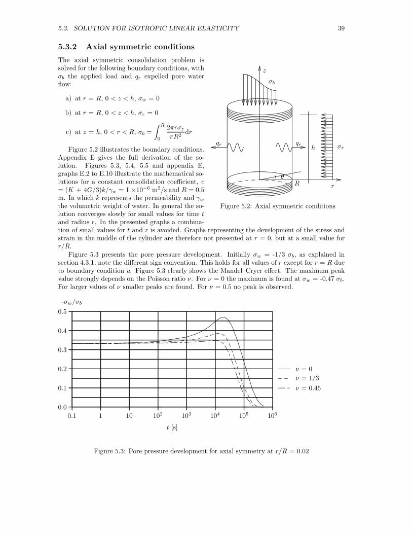
5.3. SOLUTION FOR ISOTROPIC LINEAR ELASTICITY 39
5.3.2 Axial symmetric conditions
..........................................................................................................................................................................................................................................................................................................................................................
.....
.....
.....
.....
.....
.....
.....
.....
.....
.....
.....
.....
.....
.....
.....
.....
.....
.....
.....
.....
.....
.....
.....
.....
.....
.....
.....
.....
.....
.....
.....
.....
.....
.....
.....
.....
.....
.....
.....
.....
.....
.....
.....
.....
.....
.....
.....
.....
.....
.....
.....
.....
.....
.....
.....
.....
.....
.....
.....
.....
.....
.....
.....
.....
.....
.....
.....
.....
.....
.....
.....
.....
.....
.....
.....
.....
.....
.....
.....
.....
.....
.....
.....
.......................
...................
.................................................................... ...................
................................................................................
...................
..............................................
..............................................
..............................................
.................
........................................................................................................................................................................................................................
............................................................
..........................
........................................................................
.................................................................................................................................................................................................................................................................................................................................................
........................................
............................................................................................................................................................................................................................
........................................
............................................................................................................................................................................................................................
........................................
.............................................................................................................................................................................................................................
.......................................
.............................................................................................................................................................................................................................
.......................................
............................
.........................................................................................................................................................................................................................
...........................................
.........................................................................................................................................................................................................................
...........................................
.........................................................................................................................................................................................................................
...........................................
........................................................................................................................................................................................................................
............................................
........................................................................................................................................................................................................................
............................................
........................................................................................................................................................................................................................
............................................................
..........................
..............................................................................
...........................................................................................................................................
.....
.....
.....
.
...................................................................
...............................................................................
...................
..............................................................
...............................................................................
..............
...................................................................................................................................................................
........................................................................................................................
.....
.....
....
.....
.....
.....
....
......................................................................................................................
.....
.....
....
.....
.....
.....
....
................................................................................................................
.....
.....
....
...................
......................................................................................................
.....
.....
....
.....
.....
.....
....
..........................................................................................
.....
.....
....
.....
.....
.....
....
...............................................................................
.....
.....
....
.....
.....
.....
....
.....................................................................
.....
.....
....
.....
.....
.....
....
..............................................................
.....
.....
....
.....
..............
............................................................
.....
.....
....
.....
.....
.....
....
..............................................................
...................................................................................................................................................................................................................................................................................................................................
....................
..............................................................
................................................................................
....................
.................................................................................
.................................................................................
.................................................................................
..............................................................
................................................................................
....................
..............................................................
....................................................................................................................................................................................................................................................................................................................................................................................................................
....................
..............................................................
................................................................................
....................
.....
.....
.....
.....
.....
.....
.....
.....
.....
.....
.....
.....
.....
.....
.....
.....
.....
.....
.....
.....
.....
.....
.....
.....
.....
.....
.....
.....
.....
.....
.....
.....
.....
.....
.....
.....
.....
.....
.....
.....
.....
.....
.....
.....
.....
.....
.....
.....
.....
.....
.....
.....
.....
.....
.....
.....
.....
.....
.....
.....
...
.....
.....
.....
.....
.....
.....
.....
.....
.....
.....
.....
.....
.....
.....
.....
.....
.....
.....
.....
.....
.....
.....
.....
.....
.....
.....
.....
.....
.....
.....
.....
.....
.....
.....
.....
.....
.....
.....
.....
.....
.....
.....
.....
.....
.....
.....
.....
.....
.....
.....
.....
.....
.....
.....
.....
.....
.....
.....
.....
.....
...
.....
.....
.....
.....
.....
.....
.....
.....
.....
.....
.....
.....
.....
.....
.....
.....
.....
.....
.....
.....
.....
.....
.....
.....
.....
.....
.....
.....
.....
.....
.....
.....
.....
.....
.....
.....
.....
.....
.....
.....
.....
.....
.....
.....
.....
.....
.....
.....
...............................................................
.....
.....
.....
.....
.....
.....
.....
.....
.....
.....
.....
.....
.....
.....
.....
.....
.....
.....
.....
.....
.....
.....
.....
.....
.....
.....
.....
.....
.....
.....
.....
.....
.....
.....
.....
.....
.....
.....
.....
.....
.....
.....
.....
.....
.....
.....
.....
.....
.....
.....
.....
.....
.....
..
z
rR
σb
σrhqrqr
θ
.............
.......................... ............. ............. ............. ............. ............. ............. .............
..........
Figure 5.2: Axial symmetric conditions
The axial symmetric consolidation problem issolved for the following boundary conditions, withσb the applied load and qr expelled pore waterflow:
a) at r = R, 0 < z < h, σw = 0
b) at r = R, 0 < z < h, σr = 0
c) at z = h, 0 < r < R, σb =
∫ R
0
2πrσzπR2
dr
Figure 5.2 illustrates the boundary conditions.Appendix E gives the full derivation of the so-lution. Figures 5.3, 5.4, 5.5 and appendix E,graphs E.2 to E.10 illustrate the mathematical so-lutions for a constant consolidation coefficient, c= (K + 4G/3)k/γw = 1 ×10⁻⁶ m2/s and R = 0.5m. In which k represents the permeability and γwthe volumetric weight of water. In general the so-lution converges slowly for small values for time tand radius r. In the presented graphs a combina-tion of small values for t and r is avoided. Graphs representing the development of the stress andstrain in the middle of the cylinder are therefore not presented at r = 0, but at a small value forr/R.
Figure 5.3 presents the pore pressure development. Initially σw = -1/3 σb, as explained insection 4.3.1, note the different sign convention. This holds for all values of r except for r = R dueto boundary condition a. Figure 5.3 clearly shows the Mandel–Cryer effect. The maximum peakvalue strongly depends on the Poisson ratio ν. For ν = 0 the maximum is found at σw = -0.47 σb.For larger values of ν smaller peaks are found. For ν = 0.5 no peak is observed.
0.1 1 10 102 103 104 105 106
t [s]
0.0
0.1
0.2
0.3
0.4
0.5
-σw/σb
..........................................................................................................................................................................................................................................................................................................................................
...........................................................
..................................................
............................
.........................................................................................................................................................................................................................................................................................................................................................................................................................................................................................................................
...........................................
............. ............. ............. ............. ............. ............. ............. ............. ............. ............. ............. ............. ............. ............. ............. ............. ............. ............. ............. ............. ............. ..........................
.......................... .............
............................................................................................................................................................
............. .............
............. .............
.......................... ........ .......................... ........ .......................... ........ .......................... ........ .......................... ........ .......................... ........ .......................... ........ .......................... ........ .......................... ........ .......................... ........ ............................................................
......................................................................................................
..................................
........ ..........................
.......................... ........
ν = 0
ν = 1/3
ν = 0.45
Figure 5.3: Pore pressure development for axial symmetry at r/R = 0.02

40 CHAPTER 5. 3D CONSOLIDATION
0.1 1 10 102 103 104 105 106
t [s]
0.0
0.2
0.4
0.6
0.8
1.0
1.2
............................................................................................................................................................................................................................................................................................................................................................................................................................................................................................................................................................................................................
..............................................................................................................................................................................
.................
................................................................................................................................................................................................................................................................................................................................................................
............................................................
............................................
.......................................................................................................................................................................................................
..................................................................................................................................................................................................................................................................................................................................................................................................................................................
................................................................
.......................................
..................................................................................................................................................................................................................................................
......................................................
............. ............. ............. ............. ............. ............. ............. ............. ............. ............. ............. ............. ............. ............. ............. ............. ............. ............. ............. ............. ............. ............. ............. ............. ............. .................................................................
.......................... ............. ............. .......
............. ............. ............. ............. ............. ............. ............. ............. ............. ............. ............. ............. ............. ............. ............. ............. ............. ............. ............. ............. ............. ............. ............. ............. ............. ............. ............. ............. ............. ............. ............. ............. ............. ......
............. ............. ............. ............. ............. ............. ............. ............. ............. ............. ............. ............. ............. ............. ............. ............. ............. ............. ............. ............. ............. ............. ............. ............. ............. ..........................
..........................
..........................
............. ............. .......
............. ............. .........
.......................... ........ .......................... ........ .......................... ........ .......................... ........ .......................... ........ .......................... ........ .......................... ........ .......................... ........ .......................... ........ .......................... ........ ..................................
....................................................................
.......................... ........ .......................... ...
.......................... ........ .......................... ........ .......................... ........ .......................... ........ .......................... ........ .......................... ........ .......................... ........ .......................... ........ .......................... ........ .......................... ........ .......................... ........ .......................... ........ .......................... ........ .......................... ........ ............
.......................... ........ .......................... ........ .......................... ........ .......................... ........ .......................... ........ .......................... ........ .......................... ........ .......................... ........ .......................... ........ .......................... ........ .......................... ..................................
..................................
........ .......................... ........ .........
.......................... ........ .
p′/σb
q/σb
- σw/σb
ν = 0ν = 1/3ν = 0.45
Figure 5.4: Development of p′, q and σw for axial symmetry at r/R = 0.1
Figure 5.4 presents the development of the effective isotropic stress p′, deviator stress q asdefined by equation 4.2 and σw at r/R = 0.1. These graphs show that the temporary increasein pore pressure is balanced by an increase in q and does not influence p′. The isotropic effectivestress starts to increase when the pore pressure reaches its peak value, at a higher rate for lowerν values. The deviator stress reduces finally to its initial value. Again this effect is strongest for ν= 0. For ν = 0.5 no pore pressure peak and a constant q are found.
0.1 1 10 102 103 104 105 106
t [s]
0.0
0.2
0.4
0.6
0.8
1.0
f(t)/σb
.........................................................................................................................................................................................................................................................................................................................................................................................................
..........................................................................
.....................................
.................................................................................................................................................................................................................................................................................................................................................................
...........................................
............. ............. ............. ............. ............. ............. ............. ............. ............. ............. ............. ............. ............. ............. ............. ............. ............. ............. ............. ............. ............. ............. ............. ............. ..........................
..........................
..........................
............. ............. ............. ............
............. .............
.......................... ........ .......................... ........ .......................... ........ .......................... ........ .......................... ........ .......................... ........ .......................... ........ .......................... ........ .......................... ........ .......................... ........ .......................... ........ .......................... ........ .......................... ........ .......................... ........ .............
.......................... ........
ν = 0
ν = 1/3
ν = 0.45
Figure 5.5: Development of function f(t) for axial symmetry
Section 5.2 discusses the differences between the Biot equations and the Terzaghi–Rendulicsolutions. The differences are explained in the way integration constants are handled leading toa function f(t) in absence of rotations, which is the case in a triaxial test. For ∂f(t)/∂t = 0 theBiot equations reduce to the Terzaghi–Rendulic solution. Using the expressions for e and σw givenin appendix E equation (5.3) can be used to find the expression for f(t). Figure 5.5 shows thedevelopment of f(t) for three different ν–values. Figure 5.5 clearly illustrates that condition ν =0 gives the largest change in f(t) which corresponds to the largest peak value and therefore thelargest Mandel–Cryer effect in figure 5.3. For ν = 0.45, only a minor change in f(t) is found, which

5.3. SOLUTION FOR ISOTROPIC LINEAR ELASTICITY 41
corresponds to a negligible peak in figure 5.3.
0.0 0.2 0.4 0.6 0.8 1.0
r/R
0.0
0.1
0.2
0.3
0.4
0.5-σ′r/σb ν = 0
..........................................................................................................................................................................................................................................................................................................................................................................................................................................................................................................................................................................
.................................................................................................................................................
.......................................................................................................
..............................................................................
........... ........... ........... ........... ........... ........... ........... ........... ........... ........... ........... ........... ........... ......................
......................
......................
......................
......................
...........
................ ................ ................ ................ ................ ................ ................................
................................
................................
................................
.............................
.......................... .......................... .......................... .......................... .......................... .......................... .......................... .......................... .......................... .......................... .......................... .......................... ..........................
.......................... ........ .......................... ........ .......................... ........ .......................... ........ .......................... ........ .......................... ........ .......................... ........ .......................... ........ .......................................... ........ ........ .......................... ........ ........ .......................... ........ ........ .......................... ........ ........ .......................... ........ ........ .......................... ........ ........ .......
0.0 0.2 0.4 0.6 0.8 1.0
r/R
0.0
0.1
0.2
0.3
0.4
0.5-σ′r/σb ν = 1/3
..........................................................................................................................................................................................................................................................................................................................................................................................................................................................................................................................................................................
.................................................................................................................................................
......................................................................................................
.............................................................................
........... ........... ........... ........... ........... ........... ........... ........... ........... ........... ........... ........... ........... ......................
......................
......................
......................
......................
........
................ ................ ................ ................ ................ ................ ................................
................................
................................
................................
.......................
.......................... .......................... .......................... .......................... .......................... .......................... .......................... .......................... .......................... .......................... .......................... .......................... ...................
.......................... ........ .......................... ........ .......................... ........ .......................... ........ .......................... ........ .......................... ........ .......................... ........ .......................... ........ ................................... ........ ........ .......................... ........ ........ .......................... ........ ........ .......................... ........ ........ .......................... ........ ........ .......................... ........ ........ .......
0.0 0.2 0.4 0.6 0.8 1.0
r/R
0.0
0.1
0.2
0.3
0.4
0.5-σ′r/σb ν = 0.45
..........................................................................................................................................................................................................................................................................................................................................................................................................................................................................................................................................................................
......................................................................................
.................................................................................................................................................
.......................
......................................................................................................
..................
.............................................................................
......................... ........... ........... ........... ........... ........... ........... ........... ........... ........... ........... ........... ........... ...........
......................
......................
......................
......................
.................
........... ........... ........... ........... ...................... ................ ................ ................ ................ ................ ................
................................
................................
................................
................................
....
................ ................ ................
.......................... .......................... .......................... .......................... .......................... .......................... .......................... .......................... .......................... .......................... .......................... .......................... ...............
.......................... .......................... ................
.......................... ........ .......................... ........ .......................... ........ .......................... ........ .......................... ........ .......................... ........ .......................... ........ .......................... ........ ........
.......................... ........ ..........................
.......................... ........ ........ .......................... ........ ........ .......................... ........ ........ .......................... ........ ........ .......................... ........ ........ .......................... ........ ........ .......
.......................... ........ ........ ................
t = 0t = 100 st = 1 000 st = 5 000 st = 10 000 st = 20 000 st = 50 000 st = 100 000 st = 500 000 s
Figure 5.6: Development of radial effective stress for isotropic linear elasticity and axial symmetricconditions
Appendix E, figures E.2 to E.10 present the development of all stresses and strains. The graphsillustrate the following phenomena:
effective stressFigure 5.6 presents the radial effective stress development. Initially it is found that σ′
r = σ′θ =
- 0.33 σb. It should be noted that a negative stress symbolises compression. So for a standardtriaxial compression test, with a negative value for σb, σ
′r and σ′
θ have a positive value, leading totension or a reduction in effective radial and tangential stress. For r = R the boundary conditionsimply σ′
r = 0 during the entire consolidation period. The Mandel–Cryer effect has only a minorinfluence, σ′
r and σ′θ remain virtually unaffected. The largest peak is found for ν = 0, when σ′
r,max
= σ′
θ,max = - 0.36 σb. For larger values of ν smaller peaks are found. The peak is considerablylower than the peak in pore pressure development.
total stressExpressions for total stress can either be found by a summation of the expressions for the porepressure and the effective stress or by deriving an expression directly from the consolidation equa-tion. In order to check the solutions the expressions for total stress are derived in both ways,leading to the same expression, shown in appendix E.
Initially σzz = σb except on r = R, as shown by figure 5.7. As consolidation progresses, thevertical stress increases in the middle of the cylinder while it decreases at the outer radius. Thisvisualises the redistribution of stress that takes place during consolidation. Note that boundarycondition c still holds and therefore the condition of equilibrium of forces is not violated. When σw
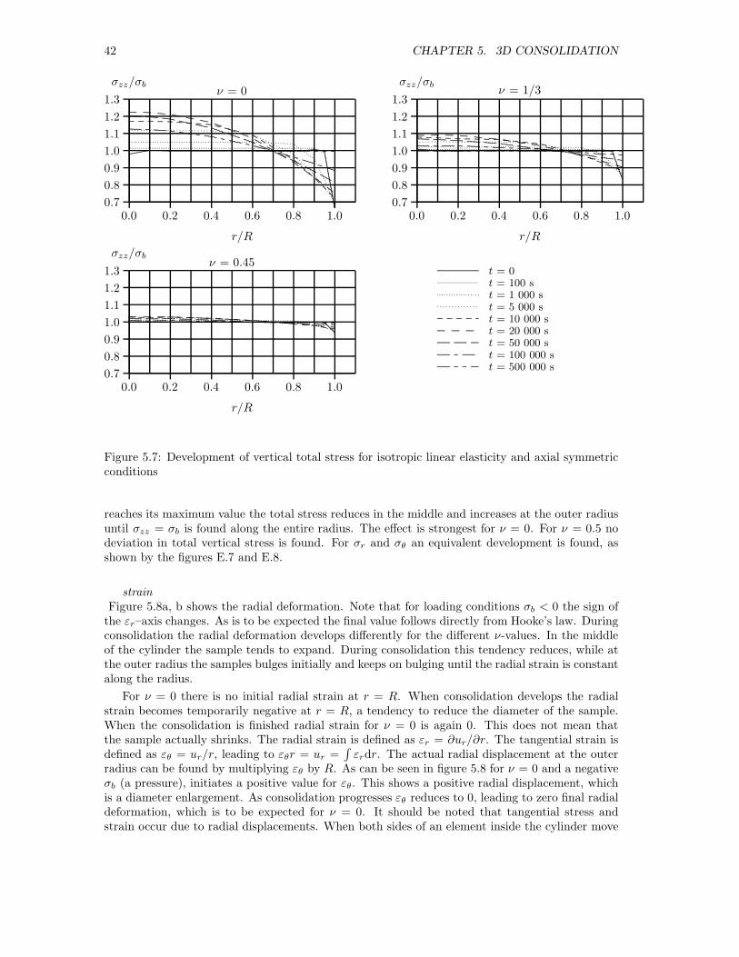
42 CHAPTER 5. 3D CONSOLIDATION
0.0 0.2 0.4 0.6 0.8 1.0
r/R
0.7
0.8
0.9
1.0
1.1
1.2
1.3
σzz/σbν = 0
.............................................................................................................................................................................................................................................................................................................................................................................................
......................................................................................................................................................
............................................................................................................................................
....................................................................................................
.............................................................................
........... ........... ........... ........... ........... ........... ........... ........... ........... ........... ........... ........... ........... ......................
......................
......................
......................
......................
...........
................ ................ ................ ................ ................ ................ ................................
................................
................................
................................
................................
.......................... .......................... .......................... .......................... .......................... .......................... .......................... .......................... .......................... .......................... ....................................................
..........................
.......................... ........ .......................... ........ .......................... ........ .......................... ........ .......................... ........ .......................... ........ .......................... ........ .......................... ........ ..................
.......................... ........ ........ .......................... ........ ........ .......................... ........ ........ .......................... ........ ........ .......................... ........ ........ .......................... ........ ........ .......
0.0 0.2 0.4 0.6 0.8 1.0
r/R
0.7
0.8
0.9
1.0
1.1
1.2
1.3
σzz/σbν = 1/3
........................................................................................................................................................................................................................................................................................................................................................................................................................................................................................
.............................................................................................................................
..........................................................................................
.......................................................................
........... ........... ........... ........... ........... ........... ........... ........... ........... ........... ........... ........... ........... ........... ........... ........... ........... ........... ........... ........... ........... ...........
................ ................ ................ ................ ................ ................ ................ ................ ................ ................ ................ ................ ................ ................ ..............
.......................... .......................... .......................... .......................... .......................... .......................... .......................... .......................... .......................... .......................... .......................... .......................... ..........
.......................... ........ .......................... ........ .......................... ........ .......................... ........ .......................... ........ .......................... ........ .......................... ........ .......................... ........ ........
.......................... ........ ........ .......................... ........ ........ .......................... ........ ........ .......................... ........ ........ .......................... ........ ........ .......................... ........ ........ .......
0.0 0.2 0.4 0.6 0.8 1.0
r/R
0.7
0.8
0.9
1.0
1.1
1.2
1.3
σzz/σbν = 0.45
........................................................................................................................................................................................................................................................................................................................................................................................................................................................
......................................................................................
....................................................................................................................
.......................
......................................................................................
..................
.....................................................................
..............
........... ........... ........... ........... ........... ........... ........... ........... ........... ........... ........... ........... ........... ........... ........... ........... ........... ........... ........... ........... ........... ........
........... ........... ........... ........... ...................... ................ ................ ................ ................ ................ ................ ................ ................ ................ ................ ................ ................ ................ ........
................ ................ ................
.......................... .......................... .......................... .......................... .......................... .......................... .......................... .......................... .......................... .......................... .......................... .......................... ........
.......................... .......................... ................
.......................... ........ .......................... ........ .......................... ........ .......................... ........ .......................... ........ .......................... ........ .......................... ........ .......................... ........ .......
.......................... ........ ..........................
.......................... ........ ........ .......................... ........ ........ .......................... ........ ........ .......................... ........ ........ .......................... ........ ........ .......................... ........ ........ .......
.......................... ........ ........ ................
t = 0t = 100 st = 1 000 st = 5 000 st = 10 000 st = 20 000 st = 50 000 st = 100 000 st = 500 000 s
Figure 5.7: Development of vertical total stress for isotropic linear elasticity and axial symmetricconditions
reaches its maximum value the total stress reduces in the middle and increases at the outer radiusuntil σzz = σb is found along the entire radius. The effect is strongest for ν = 0. For ν = 0.5 nodeviation in total vertical stress is found. For σr and σθ an equivalent development is found, asshown by the figures E.7 and E.8.
strainFigure 5.8a, b shows the radial deformation. Note that for loading conditions σb < 0 the sign of
the εr–axis changes. As is to be expected the final value follows directly from Hooke’s law. Duringconsolidation the radial deformation develops differently for the different ν-values. In the middleof the cylinder the sample tends to expand. During consolidation this tendency reduces, while atthe outer radius the samples bulges initially and keeps on bulging until the radial strain is constantalong the radius.
For ν = 0 there is no initial radial strain at r = R. When consolidation develops the radialstrain becomes temporarily negative at r = R, a tendency to reduce the diameter of the sample.When the consolidation is finished radial strain for ν = 0 is again 0. This does not mean thatthe sample actually shrinks. The radial strain is defined as εr = ∂ur/∂r. The tangential strain isdefined as εθ = ur/r, leading to εθr = ur =
∫εrdr. The actual radial displacement at the outer
radius can be found by multiplying εθ by R. As can be seen in figure 5.8 for ν = 0 and a negativeσb (a pressure), initiates a positive value for εθ. This shows a positive radial displacement, whichis a diameter enlargement. As consolidation progresses εθ reduces to 0, leading to zero final radialdeformation, which is to be expected for ν = 0. It should be noted that tangential stress andstrain occur due to radial displacements. When both sides of an element inside the cylinder move
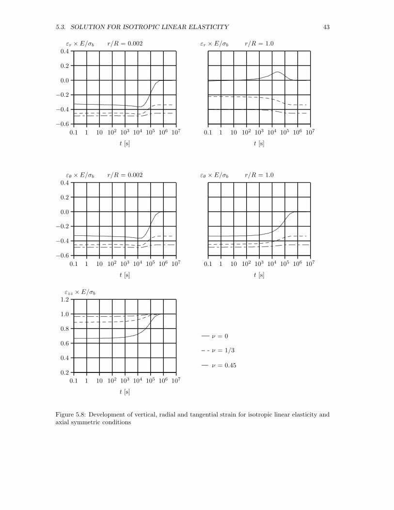
5.3. SOLUTION FOR ISOTROPIC LINEAR ELASTICITY 43
0.1 1 10 102 103 104 105 106 107
t [s]
−0.6
−0.4
−0.2
0.0
0.2
0.4εr × E/σb r/R = 0.002
..............................................................................................................................................................................................................................................................................................................................................................................................................................................................
............. ............. ............. ............. ............. ............. ............. ............. ............. ............. ............. ............. ..........................
.......................... ............. ............
.......................... ........ .......................... ........ .......................... ........ .......................... ........ .......................... ........ .......................... ........ .......................... ........ ..................
0.1 1 10 102 103 104 105 106 107
t [s]
εr × E/σb r/R = 1.0
.................................................................................................................................................................................................
.......................................
............................................................................................................................................................................
............. ............. ............. ............. ............. ............. ............. ............. ............. ............. ............. ............. ............. ............. ............. ............. ............. .....
.......................... ........ .......................... ........ .......................... ........ .......................... ........ .......................... ........ .......................... ........ .......................... ........ .................
0.1 1 10 102 103 104 105 106 107
t [s]
−0.6
−0.4
−0.2
0.0
0.2
0.4εθ × E/σb r/R = 0.002
..............................................................................................................................................................................................................................................................................................................................................................................................................................................................
............. ............. ............. ............. ............. ............. ............. ............. ............. ............. ............. ............. ..........................
.......................... ............. ............
.......................... ........ .......................... ........ .......................... ........ .......................... ........ .......................... ........ .......................... ........ .......................... ........ ..........................
0.1 1 10 102 103 104 105 106 107
t [s]
εθ × E/σb r/R = 1.0
................................................................................................................................................................................................................................
..........................................................................................................................................................................................................
............. ............. ............. ............. ............. ............. ............. ............. ............. ............. ............. ..........................
.......................... ............. ............. .....
.......................... ........ .......................... ........ .......................... ........ .......................... ........ .......................... ........ .......................... ........ .......................... ........ ..........................
0.1 1 10 102 103 104 105 106 107
t [s]
0.2
0.4
0.6
0.8
1.0
1.2εzz × E/σb
...............................................................................................................................................................................................................................
................................................................................................................................................................
............................................
..............................
............. ............. ............. ............. ............. ............. ............. ............. ............. ............. ............. ..........................
.......................... ............. ............. .............
............. ........
.......................... ........ .......................... ........ .......................... ........ .......................... ........ .......................... ........ .......................... ........ .......................... ........ ..........................
..........................
ν = 0
ν = 1/3
ν = 0.45
Figure 5.8: Development of vertical, radial and tangential strain for isotropic linear elasticity andaxial symmetric conditions

44 CHAPTER 5. 3D CONSOLIDATION
parallel to the radius, they diverge leading to tangential stress and strain. From figure 5.8 it canbe concluded that a small element at the outer radius of the cylinder is pushed outwards. Since norotational displacements occur the sides of this element, parallel to the radius, diverge leading totangential strain. At the same time the element is compressed in radial direction as ∂ur / ∂r < 0.
0.0 0.2 0.4 0.6 0.8 1.0
r/R
0.0
0.2
0.4
0.6
0.8
1.0
eE
(1 − 2ν)σbν = 0
.............................................................................................................................................................................................................................................................................................................................................................................................................................................................................................................................................................................
....................................................................................................................................................
..............................................................................................................
....................................................................................
........... ........... ........... ........... ........... ........... ........... ........... ........... ........... ........... ........... ........... .....................................................................................................................................
................ ................ ................ ................ ................ ................................
................ ...............
.................
................
................
................
................
................
................
..............
.......................... .......................... ..............................................
...... .......................... ...........
...............
................................................................................................................................................................................................................
.......................... ........ .......................... ........ .......................... ........
..........................
.................................. ........
..........................
..................................
..................................
..................................
........
.......................... ........ ........ .......................... ........ ........ .................................. ........
.......................... ........
......................
....................
.....................
.....................
..............................
.......................... .......................... ........... .......................... .......................... ........... .......................... .......................... ........... .......................... .................................................... ........ ........ ........ .......................... ........ ........ ........ .......................... ........ ........ ........ .......................... ........ ........ ........ .......................... ........ ........ .......
0.0 0.2 0.4 0.6 0.8 1.0
r/R
0.0
0.2
0.4
0.6
0.8
1.0
eE
(1 − 2ν)σbν = 1/3
................................................
...................................................................................................................................................................................................................................................................................................................................................................................................................................................................................................................................................................................................................................................................................
....................
.......................................................................................................................................................................
.........................................................................................................................................
.............. .............. ....... ....... ....... ....... ....... ....... ....... ....... ....... .............. .............. .............. ..................... .............. ....... ....................
.........................................................................................................................................................................
........... ........... ........... ........... ........... ........... ........... ........... ........... ........... ........... ........... .............................................................................................................................................................................................................
................ ................ ................ ................................
................................
................
................
................
................
................
................
................
................
................
................
................
................
................
.......................... ................................................
.............................. ............
.............. .........
.....................................................................................................................................................................................................................................................................................
.......................... ........ ..................................
..........................
.....................
.....................
..........................
..................................
..........................................
..................................
..................................
............
.......................... ........ ........ .......................... ........ ........ .................................. ........ ....................
...... ........ ........................
..................
.......................
...................
.......................
...
.......................... .......................... ........... .......................... .......................... ........... .......................... .......................... ........... .......................... ..........................
0.0 0.2 0.4 0.6 0.8 1.0
r/R
0.0
0.2
0.4
0.6
0.8
1.0
eE
(1 − 2ν)σbν = 0.45
..........................................................................................................................................................................
....................................................................................................................................................................................................................................................................................................................................................................................................................................................................................................................................................................................................................................................
......................................................................................
...........................................................................
.........................................................................................................................................
.......................
..........................................................................................................................................................
..................
.....................................................
................................................................
..............
........... ........... ........... ........... ........... ........... ........... ........... ........... ......................
......................
....................................................................................................................................................................................................................................
........... ........... ........... ........... ......
................ ................ ................ ................................
................................
................
................
................
................
................
................
................
................
................
................
................
................
................
................
......
................ ................ ................
.......................... ...............................................
...............................
..........................
........................................................................................................................................................................................................................................................................................................................
.......................... .......................... ................
.......................... ........ ..................................
.........................
. .....................
.....................
..........................
..................................
..........................................
..................................
..................................
.............
.......................... ........ ..........................
.......................... ........ ........ .......................... ........ ........ .................................. ........ .......................
... ........ ........ .......................... ........ ........ ...................
....... ........ ........ ...............
.......................... ........ ........ ................
.......................... .......................... ........... .......................... .......................... ........... .......................... .......................... ........... .......................... ..........................
.......................... .......................... .
t = 0t = 0.1 st = 100 st = 1 000 st = 5 000 st = 10 000 st = 20 000 st = 50 000 st = 100 000 st = 500 000 s
Figure 5.9: Development volumetric strain for isotropic linear elasticity and axial symmetric con-ditions

5.3. SOLUTION FOR ISOTROPIC LINEAR ELASTICITY 45
Figure 5.9 shows the volumetric strain development. When the consolidation process developsthe volumetric strain develops from the outer radius to the inner core of the cylinder. The value ofthe final volumetric strain depends strongly on the ν–value. For ν = 0 the maximum volumetricstrain is found. For ν= 0.45 the volumetric strain becomes negligible, which is to be expected sinceν = 0.5 corresponds to constant volume deformation.
5.3.3 Plane strain conditions
........................................................................................................................................................................... ...................
.............................................................................................................................................................
.....
.....
....
.....
.....
.....
....
............................
............................
.............................
.................................................
................................................
.....
.....
....
.....
.....
.....
....
..........................................................................................................................................
..................................................................................................................................................................................................................................................
..................................................................................................................................................................................................................................................
..................................................................................................................................................................................................................................................
..................................................................................................................................................................................................................................................
.....
.....
.....
.....
.....
.....
.....
.....
.....
.....
.....
.....
.....
.....
.....
.....
.....
.....
.....
.....
.....
.....
.....
.....
.....
.....
.....
.....
.....
.....
.....
...
.....
.....
.....
.....
.....
.....
.....
.....
.....
.....
.....
.....
.....
.....
.....
.....
.....
.....
.....
.....
.....
.....
.....
.....
.....
.....
.....
.....
.....
.....
.....
...
.....
.....
.....
.....
.....
.....
.....
.....
.....
.....
.....
.....
.....
.....
.....
.....
.
..............................................................................................................................................................................................................................................................
.............
.............
.....
.....
.....
.....
.....
.....
.....
.....
.....
.....
.....
.....
.....
.....
.....
.....
.....
.....
.....
.....
.....
.....
.....
.....
.....
.....
....
..........................
..........................
..........................
..........................
..........................
..........................
..........................
..........................
..........................
..........................
..........................
..........................
..........................
.........
..........................
..........................
..........................
..........................
..........................
..........................
..........................
..........................
..........................
..........................
..........................
..........................
..........................
.........
...................................................................
...............................................................................
.............. .....
..............................................................
...............................................................................
..............
.....
.....
.....
.....
.....
.....
.....
.....
.....
.....
.....
.....
.....
.....
.....
.....
.....
.....
.....
.....
.....
.....
.....
.....
.
.....................................................................
.....................................................................
.....................................................................
..................................................
...................
..................................................
...................
.....................................................................
.....................................................................
.....................................................................
..................................................
................... σx
z
xy
2F
l
qx
l
qx
h
Figure 5.10: Plane strain conditions
The plane strain consolidation problem is solved for thefollowing boundary conditions:
a) at x = 0, ∂σw/∂x =0
b) at x = l, σw = 0
c) at x = l, σxx = 0
d) at z = h, 2F/ 2l =
∫ l
−l
σzz2l
dx
Figure 5.10 illustrates the boundary conditions inwhich qx represents the expelled pore water flow. Appen-dix F gives the mathematical derivation. Graphs F.2 to
F.10 illustrate the solution for stress and strain for a consolidation coefficient, c= (K+4G/3)k/γw=1×10−6 m2/s and l = 1 m. In general it is found that the solution converges slowly for small valuesof t.
Figure 5.11 shows the pore pressure development. The presented development is equivalent tothe solution given by Mandel [57]. At x = l there is no excess pore pressure, as prescribed by theboundary conditions. At x = 0 the pore pressure initially increases. The maximum peak valuedepends on the ν - value. For ν = 0 the highest peak is found for σw = -0.58 F/l, using thesign convention according section 5.3.1. For ν = 0.5 no peak is found. Figure 5.12 presents the
1 10 102 103 104 105 106 107
t [s]
0.0
0.1
0.2
0.3
0.4
0.5
0.6
0.7
-σw × l/F
....................................................................................................................................................................................................................................................................................................................
.......................................................
..................................
.............................
.........................................................................................................................................................................................................................................................................................................................................................................................
....................................................
............. ............. ............. ............. ............. ............. ............. ............. ............. ............. ............. ............. ............. ............. .......................... ............. .............
............. ............. ............. .............
.........................................................................................................................................................................
............. ............. .............
............. ...... ...... ............. ...... ...... ............. ...... ...... ............. ...... ...... ............. ...... ...... ............. ...... ...... ............. ...... ...... ............. ...... ...... .......................................................................................................................................... ...... ...... .............
............. ...... ......
ν = 0ν = 1/3ν = 0.45
Figure 5.11: Pore pressure development for plane strain conditions at x = 0
development p′ and q, as defined by equation (4.2) and the pore pressure for x = 0. Again it isfound that the peak in pore pressure is balanced by the deviator stress. For plane strain conditionsthe final deviator stress does not equal its initial value due to the stress development in y–direction.
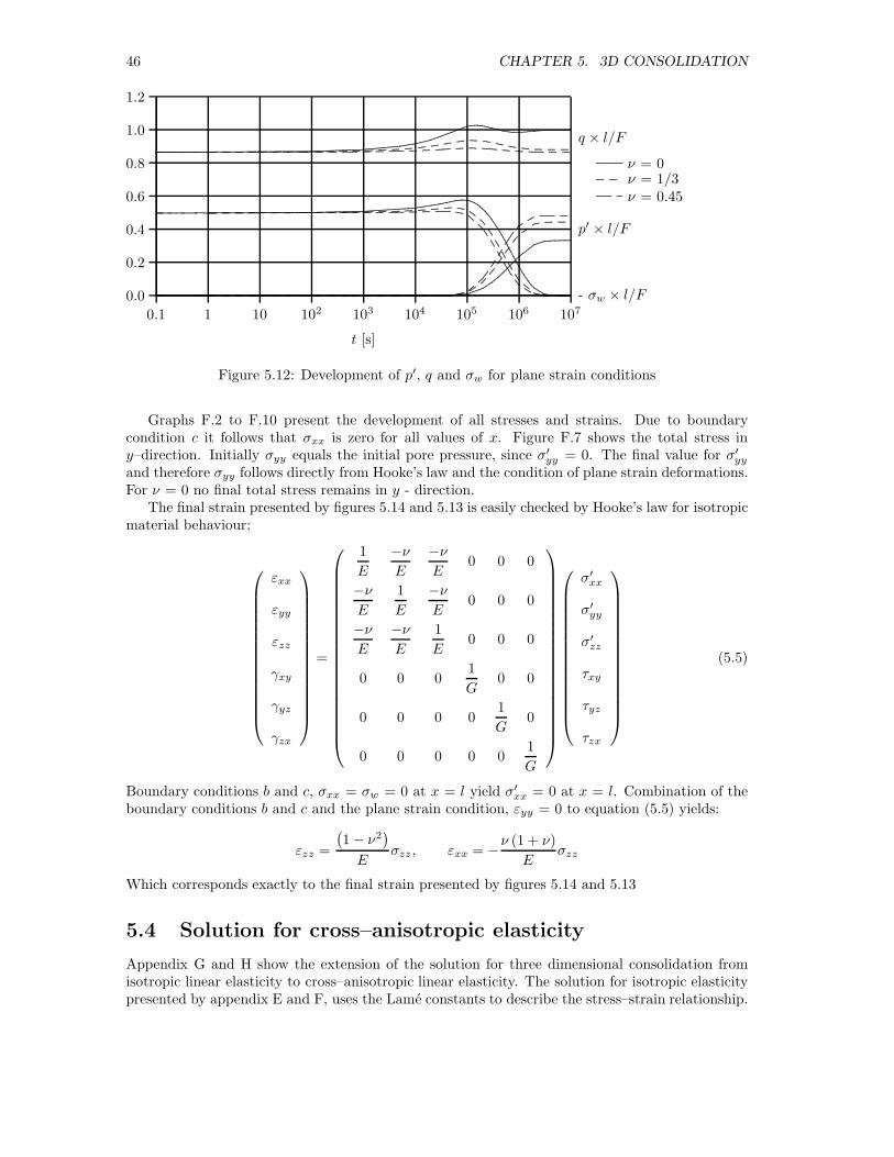
46 CHAPTER 5. 3D CONSOLIDATION
0.1 1 10 102 103 104 105 106 107
t [s]
0.0
0.2
0.4
0.6
0.8
1.0
1.2
...........................................................................................................................................................................................................................................................................................................................................................................................................................................................................................................................................................................
............................................................................................................................................................
.......................................
.....................................................................................................................................................................................................................................................................................................................................................................................................................
.........................................................
...............................
...........................
...............................
...................................................................................................................................................................................
......................................................................................................................................................................................................................................................................................................................................................................
.......................................................
......................................................................................................................................................................................................................................................................................................................
.............................................
............. ............. ............. ............. ............. ............. ............. ............. ............. ............. ............. ............. ............. ............. ............. ............. ............. ............. ............. ............. ............. ............. ............. ..........................
..............................................................................
.......................... .............
............. ............. ............. ............. ............. ............. ............. ............. ............. ............. ............. ............. ............. ............. ............. ............. ............. ............. ............. ............. ............. ............. ............. ............. ............. ............. ............. ............. ............. ............. ............. .............
............. ............. ............. ............. ............. ............. ............. ............. ............. ............. ............. ............. ............. ............. ............. ............. ............. ............. ............. ............. ............. ............. ............. ............. ..........................
.................................................................
.......................... ............. .............
............. .............
.......................... ............. ............. .......................... ............. ............. .......................... ............. ............. .......................... ............. ............. .......................... ............. ............. .......................... ............. ............. .......................... ..........................
...........................................................................................
............. .......................... .............
.......................... ............. ............. .......................... ............. ............. .......................... ............. ............. .......................... ............. ............. .......................... ............. ............. .......................... ............. ............. .......................... ............. ............. .......................... ............. ............. .......................... ............. .............
.......................... ............. ............. .......................... ............. ............. .......................... ............. ............. .......................... ............. ............. .......................... ............. ............. .......................... ............. ............. .......................... ............. .......................................
....................................................
.......................... .......................... ............. ..
.......................... ..........
p′ × l/F
q × l/F
- σw × l/F
ν = 0ν = 1/3ν = 0.45
Figure 5.12: Development of p′, q and σw for plane strain conditions
Graphs F.2 to F.10 present the development of all stresses and strains. Due to boundarycondition c it follows that σxx is zero for all values of x. Figure F.7 shows the total stress iny–direction. Initially σyy equals the initial pore pressure, since σ′
yy = 0. The final value for σ′yy
and therefore σyy follows directly from Hooke’s law and the condition of plane strain deformations.For ν = 0 no final total stress remains in y - direction.
The final strain presented by figures 5.14 and 5.13 is easily checked by Hooke’s law for isotropicmaterial behaviour;
εxx
εyy
εzz
γxy
γyz
γzx
=
1
E
−νE
−νE
0 0 0
−νE
1
E
−νE
0 0 0
−νE
−νE
1
E0 0 0
0 0 01
G0 0
0 0 0 01
G0
0 0 0 0 01
G
σ′xx
σ′yy
σ′zz
τxy
τyz
τzx
(5.5)
Boundary conditions b and c, σxx = σw = 0 at x = l yield σ′xx = 0 at x = l. Combination of the
boundary conditions b and c and the plane strain condition, εyy = 0 to equation (5.5) yields:
εzz =
(1 − ν2
)
Eσzz , εxx = −ν (1 + ν)
Eσzz
Which corresponds exactly to the final strain presented by figures 5.14 and 5.13
5.4 Solution for cross–anisotropic elasticity
Appendix G and H show the extension of the solution for three dimensional consolidation fromisotropic linear elasticity to cross–anisotropic linear elasticity. The solution for isotropic elasticitypresented by appendix E and F, uses the Lame constants to describe the stress–strain relationship.

5.4. SOLUTION FOR CROSS–ANISOTROPIC ELASTICITY 47
1 10 102 103 104 105 106 107 108
t [s]
0.4
0.6
0.8
1.0
1.2ǫzz × (El)/F
.......................................................................................................................................................................................................................................................................
.......................................
......................................................................................................................................................................................................................................................................... .................................
............. ............. ............. ............. ............. ............. ............. ............. ............. ............. ............. ............. ............. ..........................
..........................
.............
.......................... ............. ............. ...........
............. ..........
.......................... ........ .......................... ........ .......................... ........ .......................... ........ .......................... ........ .......................... ........ .................................. ..........................
........ .......................... ........ ......................
..........................
ν = 0
ν = 1/3
ν = 0.45
Figure 5.13: Development of vertical strain for plane strain conditions and isotropic linear elasticity
0.0 0.2 0.4 0.6 0.8 1.00.0
0.2
0.4
0.6
0.8
1.0
-ǫxx × (El)/Fν = 0
x/l
............................................................................................................................................................................................................................................................................................................................................................................................................................................................................................................................................
..........................................................................................................................................
.....................................................................................................
..............................................................................
........... ........... ........... ........... ........... ........... ........... ........... ........... ........... ........... ........... ........... ........... ........... ........... ........... ......................
......................
.................................
................ ................ ................ ................ ................ ................ ................ ................ ................ ................ ................................
................................
................
...............
.......................... .......................... .......................... .......................... .......................... .......................... .......................... .......................... ....................................................
....................................................
...........................
.......................... ........ .......................... ........ .......................... ........ .......................... ........ .......................... ........ .......................... ........ .......................... ..................................
..................................
.......................... ........ ........ .......................... ........ ........ .......................... ........ ........ .......................... ........ ........ .......................... ........ ........ .......................... ........ ........ ................
.......................... .......................... ........ .......................... .......................... ........ .......................... .......................... ........ .......................... .......................... ........ .......................... .......................... .............. ...... ...... ...... ...... ...... ...... ...... ...... ...... ...... ...... ...... ...... ...... ...... ...... ...... ...... ...... ...... ......
0.0 0.2 0.4 0.6 0.8 1.00.0
0.2
0.4
0.6
0.8
1.0
-ǫxx × (El)/Fν = 1/3
x/l
.......................................................................................................................................................................................................................................................................................................................................................................................................................................................................................................
................................................................................................................................
..............................................................................................
.........................................................................
........... ........... ........... ........... ........... ........... ........... ........... ........... ........... ........... ........... ........... ........... ........... ........... ........... ......................
......................
....................
................ ................ ................ ................ ................ ................ ................ ................ ................ ................ ................................
................................
................
.......................... .......................... .......................... .......................... .......................... .......................... .......................... .......................... .......................... .......................... .......................... .......................... ...................
.......................... ........ .......................... ........ .......................... ........ .......................... ........ .......................... ........ .......................... ........ .......................... ........ .......................... ........ ................
.......................... ........ ........ .......................... ........ ........ .......................... ........ ........ .......................... ........ ........ .......................... ........ ........ .......................... ........ ........ .........
.......................... .......................... ........ .......................... .......................... ........ .......................... .......................... ........ .......................... .......................... ........ .......................... .......................... .............. ...... ...... ...... ...... ...... ...... ...... ...... ...... ...... ...... ...... ...... ...... ...... ...... ...... ...... ...... ...... ......
0.0 0.2 0.4 0.6 0.8 1.00.0
0.2
0.4
0.6
0.8
1.0
-ǫxx × (El)/Fν = 0.45
x/l
..............................................................................................................................................................................................................................................................................................................................................................................................................................................................
......................................................................................
......................................................................................................................
.......................
........................................................................................
..................
......................................................................
......................... ........... ........... ........... ........... ........... ........... ........... ........... ........... ........... ........... ........... ........... ........... ........... ........... ........... ........... ........... ........... ........... ........... ........... ........... ........... ......
................ ................ ................ ................ ................ ................ ................ ................ ................ ................ ................ ................ ................ ................ ..........
................ ................ ................
.......................... .......................... .......................... .......................... .......................... .......................... .......................... .......................... .......................... .......................... .......................... .......................... .........
.......................... .......................... ................
.......................... ........ .......................... ........ .......................... ........ .......................... ........ .......................... ........ .......................... ........ .......................... ........ .......................... ........ .........
.......................... ........ ..........................
.......................... ........ ........ .......................... ........ ........ .......................... ........ ........ .......................... ........ ........ .......................... ........ ........ .......................... ........ ........ .......
.......................... ........ ........ ................
.......................... .......................... ........ .......................... .......................... ........ .......................... .......................... ........ .......................... .......................... ........ .......................... .......................... .......
.......................... .......................... ........
...... ...... ...... ...... ...... ...... ...... ...... ...... ...... ...... ...... ...... ...... ...... ...... ...... ...... ...... ...... ...... ......
...... ...... ...... ...... ......
t = 0t = 100 st = 1 000 st = 5 000 st = 10 000 st = 20 000 st = 50 000 st = 100 000 st = 500 000 st = 1 000 000 st = 5 000 000 s
Figure 5.14: Development strain in x-direction for plane strain conditions and isotropic linearelasticity
Application of the cross–anisotropic stress–strain relationship to the consolidation equation needsa reformulation of equation (3.9). This reformulation is discussed in section 3.3 and appendix B.
Appendix G gives the solution of the pore pressure development for axial–symmetric conditions,appendix H for plane–strain conditions. The appendices G and H use the same boundary conditionsand assumptions as applied in appendices E and F for the isotropic case. The graphs 5.15 and 5.16visualise the derived solutions, equations (G.29) and (H.31), for seven cases explained by table5.1. The permeability applied; k = 1 ×10⁻⁸ m/s, R = 0.5 m and l = 1 m. In section 4.3.1 it

48 CHAPTER 5. 3D CONSOLIDATION
is explained that the parameter K ′/J ′ can be used to describe the level of anisotropy. Table 5.1includes the value for K ′/J ′ for the seven cases.
Table 5.1: Seven cases for visualisation of the solutions of appendices G and Hcase Eh Ev νhh νvh K ′/J ′
[kN/m2] [kN/m2] [ - ] [ - ] [ - ]a (isotropic) 1000 1000 0 0 0b 5000 1000 0 0 0.38c 1000 5000 0 0 -0.24d 1000 1000 0 0.3 -0.11e 1000 1000 0.3 0 0.08f 5000 1000 0.3 0 0.45g 1000 5000 0 0.3 -0.29
For axial–symmetric conditions the solution converges slowly for small values for r and t. Graph5.15 shows this especially for case d.
0.1 1 10 102 103 104 105 106
t [s]
0.0
0.2
0.4
0.6
0.8
1.0
1.2
1.4-σw/σb
..............................................................................................................................................................................................................................................................................................................................
..................................................................
..................................
...........................................
..........................................................................................................................................................................................................
............. ............. ............. ............. ............. ............. ............. ............. ............. ............. ............. ..........................
...........................................................................................
................................................................................................................................................................................................................
............. .............
.......................... ........ .......................... ........ .......................... ........ .......................... ........ .......................... ........ .......................... ........ .......................... ........ .......................... ........ .......................... ........ .......................... ........ .......................... ........ .
.......................... ........ ........ .......................... ........ ........ .......................... ........ ........ .......................... ........ ........ .......................... ........ ........ .......................... ........ ........ .......................... ................
..................................
.................................. .......
.......................... .......................... ........ ........... ........... .......................... .......................... ........ ........... ........... ................................................
.... ...................
........... ....................................................
........
...........
..................................... ............
.......................... ... ..................................... ... ..................................... ...........................
............. ...........................................
........................................
.....................................
...
........................................
........................................
........................................
........................................
........................................ .
.......................... ... ... ................................................ ... ... ................................................ ... ... ................................................ ... ... ................................................ ... ... ................................................ ... ...
a
b
cd
e
f
g
Figure 5.15: Pore pressure development at r/R = 0.02 for axial–symmetric cases a to g accordingto table 5.1
The pore pressure development for cross–anisotropic conditions, shown by figures 5.15 and 5.16,differs clearly from the pore pressure development for isotropic conditions, shown by figures 5.3and 5.11. Differences are found in the initial pore pressure, the peak value and the consolidationperiod. Cross–anisotropy clearly influences the Mandel–Cryer effect. Conditions with a positiveK ′/J ′ value result in a larger initial excess pore pressure and a larger peak than conditions witha negative K ′/J ′.
The deviation of the initial σw from σw = -1/3 σb (sign convention according to section 5.3.1)for an axially loaded, cross–anisotropic sample can be explained as follows. Initially after loadingthe sample behaves undrained which means e = 0. However initial axial and radial deformations dooccur. To fulfil boundary conditions the summation of the pore pressure increase and instantaneousaxial effective stress equals the applied loading. In radial direction the summation of the porepressure increase and the instantaneous radial effective stress remain 0, since σr = 0 is prescribed

5.4. SOLUTION FOR CROSS–ANISOTROPIC ELASTICITY 49
0.1 1 10 102 103 104 105 106 107
t [s]
0.0
0.2
0.4
0.6
0.8
1.0
1.2
1.4-σw × l/F
....................................................................................................................................................................................................................................................................................................................................................................................................................................................
........................................................
............................................................................................................................................................................................................................................................................................................
............. ............. ............. ............. ............. ............. ............. ............. ............. ............. ............. ............. ............. ............. ............. ..........................
.......................................
.............
............. ..........................
.........................................................................................................................................................................
............. ............. ............. ......
.......................... ........ .......................... ........ .......................... ........ .......................... ........ .......................... ........ .......................... ........ .......................... ........ .......................... ........ .......................... ........ .......................... ........ ..................................
.......................... ........ .......................... ........ ............
.......................... ........ ........ .......................... ........ ........ .......................... ........ ........ .......................... ........ ........ .......................... ........ ........ .......................... ........ ........ .......................... ........ ........ ..................................
..................................
..........................................
................ .......................... ........
.......................... .......................... ........ ........... ........... .......................... .......................... ........ ........... ........... .......................... .......................... ........ ...................... ....
...................... ..........................
........
...........
.....................................
..................................
........... ........... .
.......................... ... ..................................... ... ..................................... ... ..................................... ... ..................................... ...
........................................
..................................... ...
........................................
........................................
........................................
........................................
..................................... ... ........................
.......................... ... ... ................................................ ... ... ................................................ ... ... ................................................ ... ... ................................................ ... ... ................................................ ... ................................................... ... ... .............
a
b
c
d
e
f
g
Figure 5.16: Pore pressure development at x = 0 for plane–strain conditions, for the cases a to gaccording to table 5.1
at r = R. The instantaneous axial and radial effective stress lead to initial, undrained, axial andradial deformations. Since e = 0, is found εzz = −2εr. For conditions with Eh > Ev a relativelylarge initial radial effective stress and a relatively small vertical effective stress are needed to fulfilthis requirement, leading to a large pore pressure increment. For Eh < Ev the opposite occurs.Now a large initial vertical effective stress and a small initial radial effective stress is needed, leadingto a low pore pressure increment.
Section 4.3.1 gives expression (4.40) for the initial pore pressure development for anisotropicconditions. To check the solutions of appendix G equation (4.40) is compared to the values foundby equation (G.29) for t = 0. To compare the two equations, equation (4.40) is rewritten into anexpression for −σw/σb, using the sign convention according to section 5.3.1. An axially loadedtriaxial test is described in terms of σa and σr by:
p =1
3(σa + 2σr)
q = σa − σr
with:
σr = 0, σa = σb
follows:
−σw0=
1
3σb +
K ′
J ′σb
−σwσb
=1
3+K ′
J ′(5.6)
For cases d and e the solution converges badly for small values of t and r. Therefore, table 5.2shows the pore pressure at t = 100 s, still relatively small, between brackets. It can be concludedthat (4.40) corresponds well to equation (G.29) for small values of t.
Figure 5.17 shows the development of f(t) for the cases a, f and g and axial symmetry. As is tobe expected the largest change in f(t) is found for case f which also gives the largest Mandel–Cryerpeak. For case g, f(t) is nearly constant which corresponds to minor Mandel–Cryer peak.
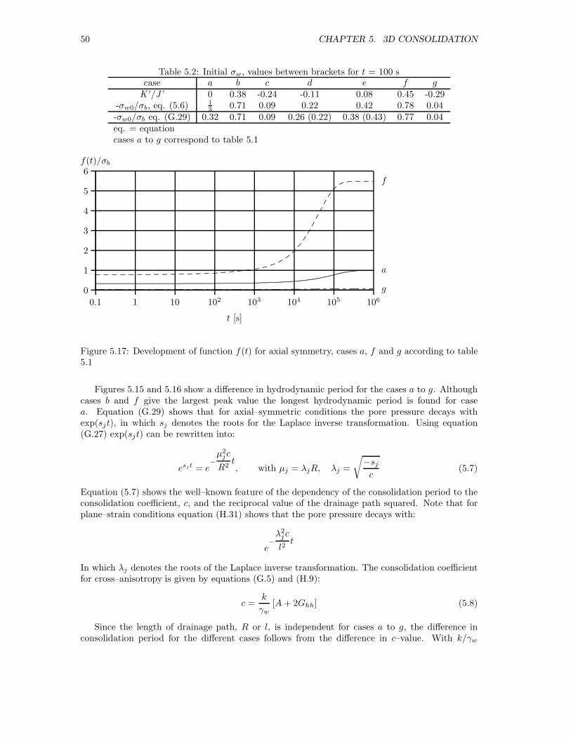
50 CHAPTER 5. 3D CONSOLIDATION
Table 5.2: Initial σw, values between brackets for t = 100 scase a b c d e f g
K’/J’ 0 0.38 -0.24 -0.11 0.08 0.45 -0.29-σw0/σb, eq. (5.6) 1
3 0.71 0.09 0.22 0.42 0.78 0.04-σw0/σb eq. (G.29) 0.32 0.71 0.09 0.26 (0.22) 0.38 (0.43) 0.77 0.04eq. = equationcases a to g correspond to table 5.1
0.1 1 10 102 103 104 105 106
t [s]
0
1
2
3
4
5
6f(t)/σb
............................................................................................................................................................................................................................................................................................................................................................................................................................................................................................................................................................................................
.............................................................
........................................
.................................................................................................
............. ............. ............. ............. ............. ............. ............. ............. ............. ............. ............. ............. ............. ............. ............. ............. ............. ............. ............. ..........................
.........................................................................................................................................................................
............. ............. ............. ............. ....
.......................... ........ .......................... ........ .......................... ........ .......................... ........ .......................... ........ .......................... ........ .......................... ........ .......................... ........ .......................... ........ .......................... ........ .......................... ........ .......................... ........ .......................... ........ .......................... ........ ............
a
f
g
Figure 5.17: Development of function f(t) for axial symmetry, cases a, f and g according to table5.1
Figures 5.15 and 5.16 show a difference in hydrodynamic period for the cases a to g. Althoughcases b and f give the largest peak value the longest hydrodynamic period is found for casea. Equation (G.29) shows that for axial–symmetric conditions the pore pressure decays withexp(sjt), in which sj denotes the roots for the Laplace inverse transformation. Using equation(G.27) exp(sjt) can be rewritten into:
esjt = e−
µ2jc
R2t, with µj = λjR, λj =
√−sjc
(5.7)
Equation (5.7) shows the well–known feature of the dependency of the consolidation period to theconsolidation coefficient, c, and the reciprocal value of the drainage path squared. Note that forplane–strain conditions equation (H.31) shows that the pore pressure decays with:
e−
λ2jc
l2t
In which λj denotes the roots of the Laplace inverse transformation. The consolidation coefficientfor cross–anisotropy is given by equations (G.5) and (H.9):
c =k
γw[A+ 2Ghh] (5.8)
Since the length of drainage path, R or l, is independent for cases a to g, the difference inconsolidation period for the different cases follows from the difference in c–value. With k/γw

5.4. SOLUTION FOR CROSS–ANISOTROPIC ELASTICITY 51
independent from the compressibility parameters the difference in consolidation coefficient is givenby the differences in A + 2Ghh, which are shown by table 5.3. Here A and Ghh are functions ofEh, Ev, νhh and νvh given in equation (3.19).
Table 5.3: Values for A and 2Ghh for the cases a to gcases a b c d e f gA 0 0 0 109.76 329.67 1648.35 18.672Ghh 1000 5000 1000 1000 769.23 3845.15 1000A + 2Ghh 1000 5000 1000 1109.76 1098.90 5494.51 1018.67
For cases b and f table 5.3 shows the value for A+2Ghh which exceeds strongly the value givenfor cases a, c, d, e and g. This corresponds to the graphs 5.15 and 5.16 in which despite the largepeak in excess pore pressure for cases b and f a shorter consolidation period is found. Case a,explained in table 5.1, acts as a set of base parameters for the cases b to g. For each of the cases bto g Eh, Ev, νhh or νvh is increased, leading to material properties which are stiffer than for casea. As is to be expected case a leads to the lowest value for A + 2Ghh and therefore to the longestconsolidation period.
0.1 1 10 102 103 104 105 106
t [s]
−0.6
−0.4
−0.2
0.0
0.2
0.4
0.6
0.8
1.0
1.2
1.4
1.6
.................................................................................................................................................................................................................................................................................................................................................................................................................................................................................................................................................................................................................................................
....................................................................................................................................................................................................................................................................................................
...................................................
............................................................................................................................................................................................
...............................................................................................................................................................................................................................................................................................................................................................
........................................................
.................................
................................................................................................................................................................................................
......................................................................................
............. ............. ............. ............. ............. ............. ............. ............. ............. ............. ............. ............. ............. ............. ............. ............. ............. ............. ............. ............. ............. ............. ............. ............. ............. ..........
............. ............. ............. ............. ............. ............. ............. ............. ............. ............. ............. ............. ............. ............. ............. ............. ............. ............. ............. ............. ............. ............. ............. ............. ............. ..........
............. ............. ............. ............. ............. ............. ............. ............. ............. ............. ............. ............. ............. ............. ............. ............. ............. ............. ............. ............. ............. ............. ............. ............. ............. ..........
............. ............. ............. .............
.......................... ........ .......................... ........ .......................... ........ .......................... ........ .......................... ........ .......................... ........ .......................... ........ .......................... ..........................................................................................................................................................................
........ ....
.......................... ........ .......................... ........ .......................... ........ .......................... ........ .......................... ........ .......................... ........
....................................................................
..................................
..................................
.................................. .......................... ........
.......................... ........ .......................... ........ .......................... ........ .......................... ........ .................................. .................
.................
..........................
....................................................................
..................................
..................................
......................................................................................................
.................................. ........
.......................... ........ ..........................
condition a
condition f
condition g
p′/σb
q/σb
-σw/σb
Figure 5.18: Development of σw, p′ and q at r/R = 0.02 for axial symmetry for the cases a, f andg
Figure 5.18 shows for two extreme cases f and g and the isotropic case, case a the developmentof p′, q and σw at r = 0. The initial value of p′ is strongly influenced by the anisotropy of the loadedsample. This can be explained by initial undrained behaviour, which means no initial volumetricstrain. As consolidation progresses p′ increases to its final value. In section 5.2 equation (4.18) ispresented:
e
εq
=
1
K ′
1
J ′
1
J ′
1
3G′
p′
q
(5.9)
For isotropic conditions 1/J ′ = 0, so e and p′ are directly coupled by the bulk modulus K ′. Foranisotropic conditions e depends on p′ as well as q. Initially after loading e remains unaffected.

52 CHAPTER 5. 3D CONSOLIDATION
Since q has an initial value equation, (5.9) predicts an initial value for p′, p′ = -(K ′/J ′) q. Table5.1 shows for case f a relatively large positive K ′/J ′ - value, resulting in a relatively large, butnegative, initial p′. When consolidation progresses p′ increases to its final value. For case g table 5.1shows a negative K ′/J ′-value. A negative K ′/J ′-value results in a positive initial p′. For case g theinitial p′ almost equals its final value which corresponds to the small amount of excess pore pressurewhich is created by axial loading as shown by figure 5.15. In section 5.3.2 it is concluded that forisotropic conditions the Mandel–Cryer effect is counterbalanced by a peak in the development of q.While p′ remains unaffected. Figure 5.18 shows that for anisotropic conditions the Mandel–Cryereffect influences q as well as p′.
5.5 Alternative conditions
With the standard solution available small changes in boundary conditions or basic assumptionseasily provide insight in the effects of alternative conditions. This section presents three of therelevant alternative conditions. The first concerns isotropically loaded samples, instead of axiallyloaded, the second involves the compressibility of the solids and the third clogging of the drain inthe triaxial test.
Isotropic loading
0.1 1 10 102 103 104 105 106
t [s]
0.0
0.2
0.4
0.6
0.8
1.0
1.2
1.4
1.6
1.8-σw/σb
........................................
..........................................
.........................................................................
.........................................................................................................................................................................................................................................................................................
..........................................................................
........................................
....................................................................................................................................................................................................................................................................................................................................................................................................................................................................................................................................................................................................................................................................
............. ............. ............. ............. ............. ............. ............. ............. ............. ............. ............. ............. ............. ..........................
.....................................................................................................................
........................................................................................................................................................................................................................................................................................................... ............. ............. .......
.......................... ........ .......................... ........ .......................... ........ .......................... ........ .......................... ........ .......................... ........ .................................. ......................
.... ......................
....................
..................................
............................................................
............................................................................................................................................................................................................
........ ..........................
.......................... ........ ........ .......................... ........ ........ .......................... ........ ........ .......................... ........ ........ .......................... ........ ........ .................................. ........
..........................
................
..........................
..........................................
........................................................................................................................................................................................
.......................... ........ .....
.......................... .......................... ........ ........... ........... .................................................... ........ ........... ........... ......................
.... .......................... ........
...........
.......................................................................
...........
.......................................................................
...........
.......................................................................
...........
.....................................
.......................... ...
.......................... ... ..................................... ... ..................................... ... .....................................
....................
....................
...
........................................
........................................
.....................................
...
........................................
........................................
........................................
........................................
........................................
........................................
..................................... ...
.......................... ... ... ................................................ ... ... ................................................ ... ... ................................................... ... ....................
............................
......
................................................ ...
...
......................................................
......................................................
......................................................
................................................ ... ...
a
b
c
d
e
f
g
Figure 5.19: Pore pressure development at r/R = 0.1 for axial symmetric conditions and isotropicloading, cases a to g according to table 5.1
Appendix H gives the boundary conditions in terms of g1, g2 and g3. In which g1 representsthe pore pressure prescribed at r = R, g2 represents σr prescribed at r = R and g3 represents σzzprescribed at z = h. For g2 = g3 = σb consolidation due to an isotropic load is modelled. Figure5.19 visualises the results. Again a radial pore pressure dissipation is assumed in combination toa stiff plate on top. The solution is shown for the seven cases presented in table 5.1. Now for eachcase the initial pore pressure equals the initial loading, -σw/σb = 1. This corresponds to equation

5.5. ALTERNATIVE CONDITIONS 53
(4.40) since for isotropic loading q = 0 and p = σb. Especially for case d the solution convergesbadly for small values for t and r. Figure 5.19 shows the short consolidation period for cases b andf and shows the Mandel–Cryer effect clearly for all cases a to g. Even for cases c and g the peak isconsiderable, -σw/σb up to 1.26. Figure 5.19 shows that a large peak value is found for Eh > Ev,while for Ev > Eh the peaks are smaller.
Compressible solids
Appendix I gives the derivation for the three–dimensional axial symmetric consolidation includingcompressible solids. To give a clear view on the individual phenomena that play a role the solutionfor isotropic material behaviour is extended to compressible solids. Chapter 2 discusses the differentcompression moduli. Barends [7] gives the storage equation including the solid stiffness. Figure5.20 shows the results for three cases, each with ν = 0, E = 1000 kPa, (β = 0.003 1/kPa, K =333.33 kPa), porosity n = 0.4 and permeability k = 1×10⁻⁸ m/s. The condition βsf = βss = 0corresponds to case a in figure 5.15 and ν = 0 in figure 5.3. To show the influence of the differentcompressibility parameters to the pore pressure development for the second case only compressiondue to inter granular contacts is considered while the solids remain incompressible for a deviationin isotropic stress; βss = 0.5β, βsf = 0. The third case presents the opposite condition, βsf = 0.5β,βss = 0. Figure 5.20 shows the influence of the parameters βss and βsf . Compression due to inter
0.1 1 10 102 103 104 105 106
t [s]
0.0
0.1
0.2
0.3
0.4
0.5
0.6
-σw/σb
.....
.....
.....
.....
.....
.....
.....
.....
.....
.....
.....
.....
.....
.....
.....
.....
.....
.....
.....
.....
.....
.....
.....
.....
.....
.....
.....
.....
.....
.....
.....
.....
.....
.....
.....
.....
.....
.....
.....
.....
.....
.....
.....
.....
.....
.....
.....
.....
.....
.....
.....
.....
.....
.....
..
t = 16 000 s
t = 12 000 s
t = 20 000 s
...................................................................................................................................................................................................................................................................................................................................................
..........................................................
..............................................
....................................................................................................................................................................................................................................................................................................................................................................................................................................................................................................................................................................................
...........................................
............. ............. ............. ............. ............. ............. ............. ............. ............. ............. ............. ............. ............. ............. ............. ............. ............. ............. ............. .................................................................
.............
..........................
......................................................................................................................................................................................
............. ............. ............. .
............. .............
.......................... ........ .......................... ........ .......................... ........ .......................... ........ .......................... ........ .......................... ........ .................................. ..........................
........ ..........................
..................................
..........................................
........................................................................................................................................................................................................................................................................
.................................. ........ .........
.......................... ........
βss = βsf = 0
βss = 0.5β, βsf = 0
βss = 0, βsf = 0.5β
Figure 5.20: Pore pressure development for isotropic material behaviour including compressiblesolids for axial symmetry at r/R = 0.1, ν = 0, E = 1000 kPa, n = 0.4 and k = 1×10⁻⁸ m/s
granular contacts, βss causes a slight acceleration in the consolidation process. Figure 5.20 showsa maximum peak value after 12 000 s, while for the condition with incompressible solids the peakis found at 20 000 s. The shape of the pore pressure development remains unaffected by βss. Theinitial value, the maximum peak and the slope of the pore pressure development after the peakare equal to those for the incompressible solids. The compressibility due to isotropic stress, βsfcauses a change in shape of the pore pressure development. A larger initial pore pressure, a largerpeak value up to −σw/σb = 0.57, and a steeper slope after the maximum value are found. Themaximum value is found at 16 000 s, indicating acceleration of the consolidation process. Note thatβsf has the same type of influence on the consolidation process as cross–anisotropy for K ′/J ′ > 0.Both lead to a larger initial pore pressure and a larger peak value.
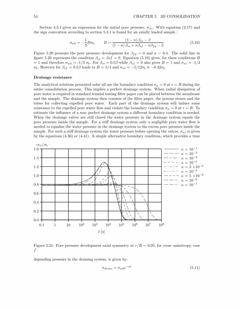
54 CHAPTER 5. 3D CONSOLIDATION
Section 4.3.1 gives an expression for the initial pore pressure, σwi. With equation (2.17) andthe sign convention according to section 5.3.1 is found for an axially loaded sample :
σw0 = −1
3Bσb, B =
(1 − n)βss − β
(1 − n)βss + nβsf − nβfg − β(5.10)
Figure 5.20 presents the pore pressure development for βfg = 0 and n = 0.4. The solid line infigure 5.20 represents the condition βss = βsf = 0. Equation (5.10) gives, for these conditions B= 1 and therefore σw0 = -1/3 σb. For βss = 0.5β while βsf = 0 also gives B = 1 and σwi = -1/3σb. However for βsf = 0.5β leads to B = 5/4 and σwi = −5/12σb ≈ −0.42σb.
Drainage resistance
The analytical solutions presented sofar all use the boundary condition σw = 0 at r = R during theentire consolidation process. This implies a perfect drainage system. When radial dissipation ofpore water is required in standard triaxial testing filter paper can be placed between the membraneand the sample. The drainage system then consists of the filter paper, the porous stones and thetubes for collecting expelled pore water. Each part of the drainage system will induce someresistance to the expelled pore water flow and violate the boundary condition σw = 0 at r = R. Toestimate the influence of a non–perfect drainage system a different boundary condition is needed.When the drainage valves are still closed the water pressure in the drainage system equals thepore pressure inside the sample. For a stiff drainage system only a negligible pore water flow isneeded to equalise the water pressure in the drainage system to the excess pore pressure inside thesample. For such a stiff drainage system the water pressure before opening the valves, σwi is givenby the equations (4.36) or (4.41). A simple alternative boundary condition, which provides a time
0.1 1 10 102 103 104 105 106 107 108
t [s]
0.0
0.2
0.4
0.6
0.8
1.0
1.2
1.4
1.6-σw/σb
.....................................................................................................................................................................................................................
.........................................
.............................
.....................................................................................................................................................................................................................................................................................................................................................................................................................................................................................................................................................................................................................................................................................................................................................................................................................................................................
..............................................................................................
.......................... .......................... .......................... .......................... .......................... .......................... ..........................................
....................................
..................................................................................................................................
....................................................................................................................................................................................................................................................................
.......................... .......................... .......................... .......................... .......................... .......................... .......................... ........
.......................... .......................... ........................
.......................... ............. .......................... ............. .......................... ............. .......................... ............. .......................... ............. ..........................
..................................................................................................................... .............
.............................................................................................................................................................................................................................
....................................... ............. .......................... ............. .......................... ............. .......................... ............. .............
.......................... ............. .......................... ..
............. ............. ............. ............. ............. ............. ............. ............. ............. ............. ............. ............. ............. ..........................
.............
.......................................
.............
.............
.............
.............
.............
.............
.............
.............
.............
.............
.............
.............
.......................... ............. ............. ............. ............. ............. ............. ............. ............. .......
............. ............. ............. .............
............. ...... ............. ...... ............. ...... ............. ...... ............. ...... ............. ...... ............. ...... ............. ...... ............. ...... ............. ...... ................................................... ......
..................................................................................................................................................
...... ............. ...... ............. ...... ............. ...... ............. ...... ............. ...... .............
............. ...... ............. ...... .............
............. ...... ...... ............. ...... ...... ............. ...... ...... ............. ...... ...... ............. ...... ...... ............. ...... ...... ............. ...... ...... ............. ...... ...... ................... ...... .............
............................................................................................................................. ...... ...... ............. ...... ...... ............. ...... ...... ............. ...... ..
............. ...... ...... ............. ...... ....
.......................... ............. ............. .......................... ............. ............. .......................... ............. ............. .......................... ............. ............. .......................... ............. ............. ....................................... ............. ..........................
..................................................................................................................................
.......................... ............. ............. .......................... ............. ............. ..........................
.......................... ............. ............. ..............
.......................... .......................... ............. .......................... .......................... ............. .......................... .......................... ............. .......................... .......................... ............. .......................... .......................... ............. .......................... .......................................
....................................................
.......................................
.................................................................
.......................... ............. .......................... .......................
.......................... .......................... ............. ..
.......................... .......................... ............. ............. .......................... .......................... ............. ............. .......................... .......................... ............. ............. .......................... .......................... ............. ............. .......................... .......................... ............. ............. ....................................................
....................................................
..............................................................................
.......................... .....
.......................... .......................... ............. ..
κ = 10−1
κ = 10−2
κ = 10−3
κ = 10−4
κ = 5 ×10⁻⁵
κ = 10−5
κ = 5 ×10⁻⁶
κ = 10−6
κ = 10−7
Figure 5.21: Pore pressure development axial symmetry at r/R = 0.05, for cross–anisotropy, casef
depending pressure in the draining system, is given by:
σdrain = σw0e−κt (5.11)
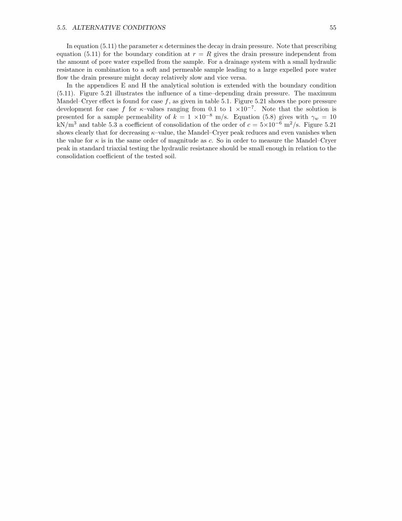
5.5. ALTERNATIVE CONDITIONS 55
In equation (5.11) the parameter κ determines the decay in drain pressure. Note that prescribingequation (5.11) for the boundary condition at r = R gives the drain pressure independent fromthe amount of pore water expelled from the sample. For a drainage system with a small hydraulicresistance in combination to a soft and permeable sample leading to a large expelled pore waterflow the drain pressure might decay relatively slow and vice versa.
In the appendices E and H the analytical solution is extended with the boundary condition(5.11). Figure 5.21 illustrates the influence of a time–depending drain pressure. The maximumMandel–Cryer effect is found for case f , as given in table 5.1. Figure 5.21 shows the pore pressuredevelopment for case f for κ–values ranging from 0.1 to 1 ×10⁻⁷. Note that the solution ispresented for a sample permeability of k = 1 ×10⁻⁸ m/s. Equation (5.8) gives with γw = 10kN/m3 and table 5.3 a coefficient of consolidation of the order of c = 5×10⁻⁶ m2/s. Figure 5.21shows clearly that for decreasing κ–value, the Mandel–Cryer peak reduces and even vanishes whenthe value for κ is in the same order of magnitude as c. So in order to measure the Mandel–Cryerpeak in standard triaxial testing the hydraulic resistance should be small enough in relation to theconsolidation coefficient of the tested soil.

56 CHAPTER 5. 3D CONSOLIDATION

Chapter 6
Laboratory measurements
6.1 Tests on peat
Chapters 3 to 5 discuss a mathematical description of anisotropy and the influence of anisotropyto consolidation behaviour. As explained in chapter 1 behaviour of peat forms the main objectiveof this study. This chapter discusses measurements on the consolidation behaviour of peat andcompares the results to the analytical solutions presented in chapter 5.
There are three optional causes for peat to behave anisotropically. First, anisotropy can bedue to the structure of peat. The stiffness in the main fibre direction differs from the stiffnessperpendicular to the fibres. This is known as structural anisotropy. It is assumed that the fibresare mainly oriented in the horizontal plane, which leads to a difference in stiffness in horizontaland vertical direction. The second optional cause is a load-induced anisotropy. Since peat is asoft and compressible material the stiffness depends on the stress level or even on the rate ofcompression. A deviator load will induce a difference in compressibility in different directions andtherefore a difference in stiffness. The third option originates from a difference in loading andunloading conditions. Section 4.2 explains that true elastic behaviour is only found at very smallstrain level. Exceeding this small strain level already leads to residual deformation. In engineeringpractice equivalent elastic moduli, which include some plastic deformation, are used. This workingmethod implies a difference in stiffness moduli for loading and unloading conditions. Loading anundrained soil sample in the axial direction gives an effective stress increase in axial direction anda decrease in radial effective stress due to generation of pore pressure. So even for isotropic soilanisotropic behaviour can be found. According to Parry & Wroth [62] this is referred to as stressanisotropy.
This chapter first gives a characterisation of the tested material in section 6.2. Special attentionis given to the axial pre–consolidation stress discussed in section 6.2.3. Section 6.3 discussesmeasurements of the shear modulus, for small strain using bender elements and moderate to largestrain using simple shear tests. Chapter 2 deals with the compressibility of the individual phases inrelation to the Skempton B–factor. Section 6.5 discusses measurements of the Skempton B–factorin combination with the degree of saturation. Chapter 5 shows that the influence of anisotropyis found in the undrained effective stress path and in the Mandel–Cryer effect. Section 6.6 showsmeasurements of the effective stress path for small undrained loading steps at different levels ofpre–consolidation. Section 6.7 shows measurements on the Mandel–Cryer effect.
57

58 CHAPTER 6. LABORATORY MEASUREMENTS
6.2 Characterisation of tested soil
6.2.1 Sample location
Figure 6.1: Sample location
The samples are retrieved near Breukelenalong the highway A2 near the future junc-tion Breukelen - Vinkeveen. Due to the re-construction of the highway a field surveyis conducted. The soil consists of an ap-proximately 6 m thick peat layer on top ofa thick Pleistocene sand layer. The groundwater table ranges between 0.6 and 0.3 mbelow surface. The samples are retrievedhorizontally as well as vertically. Photo 6.1shows that the vertically retrieved samplesare taken at a depth of approximately 1m below surface level, 0.7 to 0.4 m belowphreatic level, using a sampling tube withlength of 440 mm and diameter of 66 mm.The lower part of the tubes, used for retriev-ing samples in vertical direction, reached athin clayey layer. This part of the samplematerial is disregarded. After retrieving thesamples the tubes are sealed and stored in atemperature and humidity controlled room.
Each sampling tube has a unique num-ber. The sample number corresponds tothe sampling tube number by which it isretrieved followed by an a, b, c, etc. for thefirst, second, third, etc. sample taken fromthis sampling tube. When discussing the
measurement results these numbers are mentioned in following sections.
6.2.2 Descriptive parameters
To have a good impression of the tested material several descriptive parameters have been derivedfrom the samples or from parts cut off when trimming.
The water content W is defined as the ratio of pore water mass Mw and mass of dry solidparticles Ms:
W =Mw
Ms
(6.1)
The value for Ms is determined after heating the sample to 105◦ C during 24 hours. Skempton &Petley [66] conclude that the loss on organic matter is insignificant when temperatures up to 105◦
C are used, while for lower temperatures, 60 to 85◦ C small amounts of free pore water remain.The difference in mass before and after drying the sample gives the pore water mass. Since peatcontains a large amount of pore water and the solids have a relatively low density, compared tosand or clay, the pore water mass easily exceeds the mass of solid material. Typical values of Wfor peat ranges from 2 to 10.
The loss on ignition N presents the material content that evaporates when heated to a largetemperature. Several authors and standard regulations give small differences in the prescription

6.2. CHARACTERISATION OF TESTED SOIL 59
for the determination of N [66]. The values presented in table 6.1 are found after heating thesample to 500◦ C during 4 hours. With m1 the remaining mass of the sample, N is given by:
N =Ms −m1
Ms
(6.2)
The organic content P , the ratio of mass of organic material to total mass is close to N , (6.2).Skempton & Petley [66] present a correlation between N and P :
P = 1 − 1.04 (1 −N) (6.3)
The ash content is the complement of the organic content. Based on equation (6.3) is found:
ash content = 1.04 (1 −N) (6.4)
Equation (6.4) indicates that during heating the anorganic part looses 4% of its mass. For a largeorganic content, a small ash content, this is a negligible error in comparison to the natural hetero-geneity of peat. This results in equating P to N for typical peat conditions [25].
The solid density ρs is found by using an automated pycnometer method according to theDutch regulations NEN5111 [58]. The standard pycnometer method uses the difference in mass ofa fluid with a known density, e.g. water and the mass of the same volume of the tested materialsaturated with this fluid. The solid density presented in tables 6.1 and 6.6 are found using helium.
Skempton & Petley [66] show a strong correlation between the organic content and the specificgravity of solidsGs in which Gs is defined asGs = ρs/ρw. For soil types in Western Europe withoutany organic material Gs is of the order of 2.65. Pure organic material has a specific gravity of Gsof the order of 1.4. For intermediate values of the organic content Gs has some intermediate value.With P = N is found:
1
Gs=
N
1.4+
1 −N
2.65(6.5)
Den Haan et al [25] show that equation (6.5) applies well for Dutch soils.
Total density ρ is given by the initial sample dimensions and mass. This provides the initialdensity ρ for each test. The total density is a useful parameter in several correlations ([25], [24])and for differentiating different types of peat as explained in [69].
Using weight and volume of samples used for the triaxial tests discussed in the following sections,the void ratio e, porosity n and initial degree of saturation Sri can be found by the followingequations:
e =VpVs
=Gsρw − ρd
ρd
ρd =ρ
1 +W
n = 1 − ρdGsρw
Sr =Wρ
nρw (1 +W )=GsW
e=ρ− (1 − n) ρs
nρw
(6.6)
In which:
Vp = pore volumeVs = volume solidsρd = dry density, Ms/VV = total soil volume
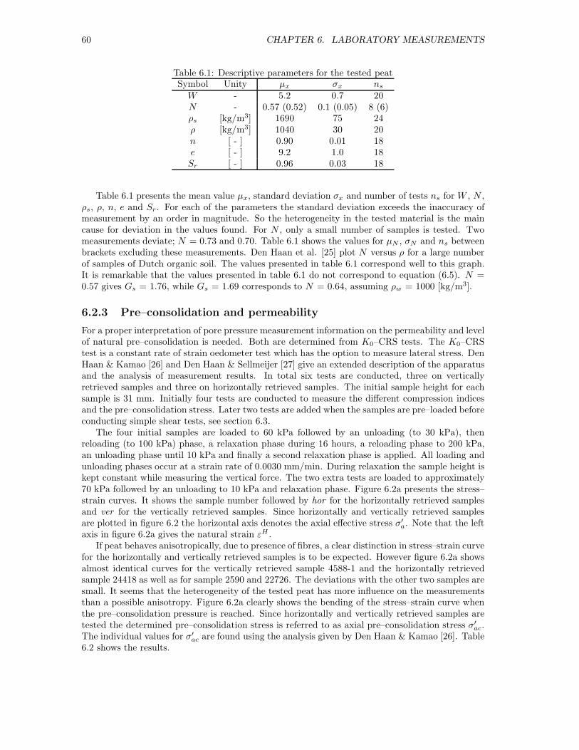
60 CHAPTER 6. LABORATORY MEASUREMENTS
Table 6.1: Descriptive parameters for the tested peatSymbol Unity µx σx nsW - 5.2 0.7 20N - 0.57 (0.52) 0.1 (0.05) 8 (6)ρs [kg/m3] 1690 75 24ρ [kg/m3] 1040 30 20n [ - ] 0.90 0.01 18e [ - ] 9.2 1.0 18Sr [ - ] 0.96 0.03 18
Table 6.1 presents the mean value µx, standard deviation σx and number of tests ns for W , N ,ρs, ρ, n, e and Sr. For each of the parameters the standard deviation exceeds the inaccuracy ofmeasurement by an order in magnitude. So the heterogeneity in the tested material is the maincause for deviation in the values found. For N , only a small number of samples is tested. Twomeasurements deviate; N = 0.73 and 0.70. Table 6.1 shows the values for µN , σN and ns betweenbrackets excluding these measurements. Den Haan et al. [25] plot N versus ρ for a large numberof samples of Dutch organic soil. The values presented in table 6.1 correspond well to this graph.It is remarkable that the values presented in table 6.1 do not correspond to equation (6.5). N =0.57 gives Gs = 1.76, while Gs = 1.69 corresponds to N = 0.64, assuming ρw = 1000 [kg/m3].
6.2.3 Pre–consolidation and permeability
For a proper interpretation of pore pressure measurement information on the permeability and levelof natural pre–consolidation is needed. Both are determined from K0–CRS tests. The K0–CRStest is a constant rate of strain oedometer test which has the option to measure lateral stress. DenHaan & Kamao [26] and Den Haan & Sellmeijer [27] give an extended description of the apparatusand the analysis of measurement results. In total six tests are conducted, three on verticallyretrieved samples and three on horizontally retrieved samples. The initial sample height for eachsample is 31 mm. Initially four tests are conducted to measure the different compression indicesand the pre–consolidation stress. Later two tests are added when the samples are pre–loaded beforeconducting simple shear tests, see section 6.3.
The four initial samples are loaded to 60 kPa followed by an unloading (to 30 kPa), thenreloading (to 100 kPa) phase, a relaxation phase during 16 hours, a reloading phase to 200 kPa,an unloading phase until 10 kPa and finally a second relaxation phase is applied. All loading andunloading phases occur at a strain rate of 0.0030 mm/min. During relaxation the sample height iskept constant while measuring the vertical force. The two extra tests are loaded to approximately70 kPa followed by an unloading to 10 kPa and relaxation phase. Figure 6.2a presents the stress–strain curves. It shows the sample number followed by hor for the horizontally retrieved samplesand ver for the vertically retrieved samples. Since horizontally and vertically retrieved samplesare plotted in figure 6.2 the horizontal axis denotes the axial effective stress σ′
a. Note that the leftaxis in figure 6.2a gives the natural strain εH .
If peat behaves anisotropically, due to presence of fibres, a clear distinction in stress–strain curvefor the horizontally and vertically retrieved samples is to be expected. However figure 6.2a showsalmost identical curves for the vertically retrieved sample 4588-1 and the horizontally retrievedsample 24418 as well as for sample 2590 and 22726. The deviations with the other two samples aresmall. It seems that the heterogeneity of the tested peat has more influence on the measurementsthan a possible anisotropy. Figure 6.2a clearly shows the bending of the stress–strain curve whenthe pre–consolidation pressure is reached. Since horizontally and vertically retrieved samples aretested the determined pre–consolidation stress is referred to as axial pre–consolidation stress σ′
ac.The individual values for σ′
ac are found using the analysis given by Den Haan & Kamao [26]. Table6.2 shows the results.

6.2. CHARACTERISATION OF TESTED SOIL 61
0.1 1 10 100 1000
σ′a [kPa]
1.0
0.9
0.8
0.7
0.6
0.5
0.4
0.3
0.2
0.1
0
εH
(hor) = horizontally retrieved sample(ver) = vertically retrieved sample
a
..............................................................................................................................................................................................................................................................................................................................................................................................................................................................................................................................
........................
....................
...................
..................
.................
..................
.........................
..................................................................................................................................................................................................................................................................................................................................................................................................................................................................................................................................................................................................................
.........................
.....................
.................
.................
..................
..................
.................................
.....................................................................................................................................................................................................................................................................................................................................................................................
.....................
...................
.................................
..................................................................................................................................................................................................................................................................................................................................................................................................................................................................................................................................................................................................................................................................................................................................................................................................................................................................
....................................
.......................
..................
...................
..................
...................
.................................................
.....................................................................................................................................................................................................................................................................................................................................................................................................................................................................................................................................................................................................................................................
................................
.............................
...........................
..........................
..............................................
.........................................................................................................................................................................................................................................................................................................................................................................................................
......................
...................
................................
4588-1, (ver)24418, (hor)
4588-2, (ver)24505, (hor)2590, (ver)
22726, (hor)
0.1 1 10 100 1000
σ′a [kPa]
0.0
0.2
0.4
0.6
0.8
1.0
1.2
1.4
1.6
1.8
2.0
K0
b
...............................................................................................................................................................................
................................................................................
.......................................................
.........................................................................
.....................................................................................................................................................................................................................................................................................................................................................................................
.....
......
.....
.....
.....
..................................................................................
............................................................................
..............................................................................
...........................................................................................................................................................................................................................................................................................................................................................................................................................
...................................................................................................................................................
..................................................
..............................................................................................................................................................................................................................................................................................................
....................................................................................................................................................................................................................................................................................................................................................................................................................................................................................................................................................
...................................................................................................................
.............................................................................................................................................................................................................................................................................................................................................................................................................................................................................................................
..............................................................................................................................
.......................................................................................................................................
..................................................................................
..............................................................................
4588-1, (ver)
24418, (hor)
4588-2, (ver)
24505, (hor)
2590, (ver)
22726, (hor)
Figure 6.2: Results on 6 K0–CRS tests, a) stress–strain development b) σ′a–K0 development
Table 6.2: Results of the K0 − CRS testsSample σ′
ac K0 χ k0
nr [kPa] [ - ] [ - ] [m/s]4588-1 (ver) 11.9 0.36 4.34 1.6 ×10⁻⁸
4588-2 (ver) 16.7 0.29 5.28 2.8 ×10⁻⁸
2590 (ver) 21.8 0.26 5.10 3.2 ×10⁻⁸
24505 (hor) 20.8 0.36 5.26 2.1 ×10⁻⁸
24418 (hor) 11.5 0.36 4.56 2.3 ×10⁻⁸
22726 (hor) 19.1 0.32 5.28 2.8 ×10⁻⁸
with χ and k0 defined by equation (6.7)
Using the density presented in table 6.1 and the position of the water table the vertical effectivestress in the field σ′
v0 can be estimated. Since the water table is between 0.3 and 0.6 m below surfaceσ′v0 ranges from 4 to 7 [kPa]. Several phenomena might explain the difference in σ′
ac and σ′v0 like
fluctuation of the water table, oxidation of the top layer or aging.Figure 6.2b shows K0 versus σ′
a, in which K0 is defined as the ratio of radial effective stress toaxial effective stress, σ′
r/σ′a. Again it is to be expected that if the fibres are aligned in one plane
and if the fibres play an important role in the stiffness characteristics of peat a clear differencebetween the horizontally and vertically retrieved samples is to be expected. Figure 6.2b showsequivalent behaviour for the six samples. Again heterogeneity of the peat samples seems moreimportant than a possible anisotropy of peat.
During execution of the tests the pore pressure is measured at the bottom of the sample. Themeasurement data is used to assess the permeability according to the analysis given by Den Haanet al [28]. The results of the loading phases are used to fit the relation:
k = k0 × exp (−χe) (6.7)
Table 6.2 shows the results. Note that the values for k0 are remarkably low regarding the largeporosity found in table 6.1, n = 0.9. Possibly this can be explained by a relatively large amount
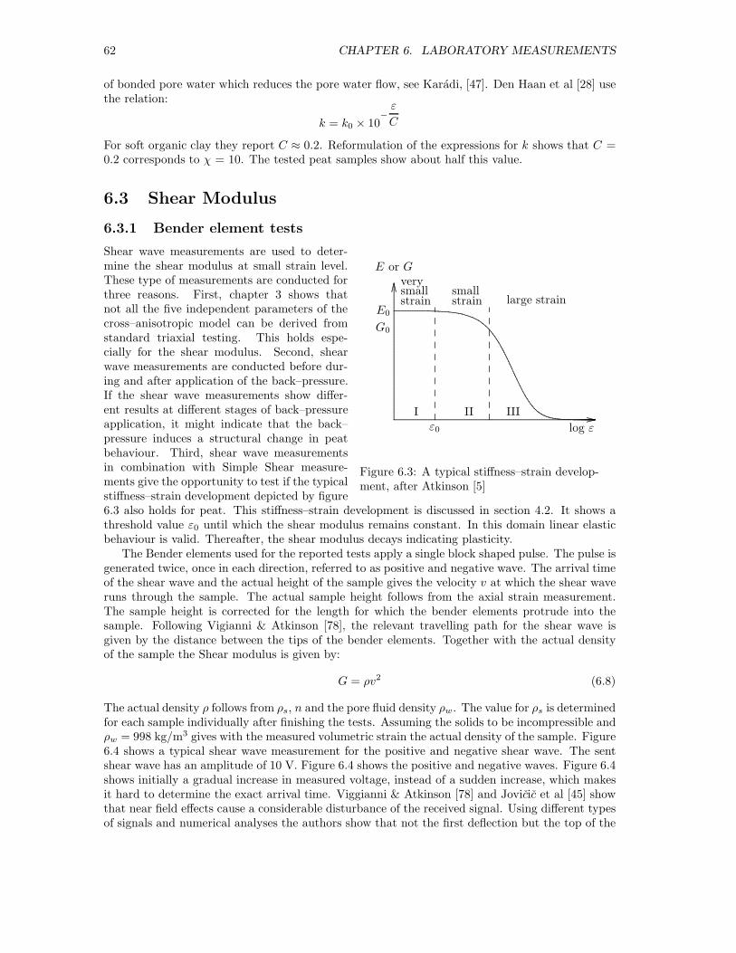
62 CHAPTER 6. LABORATORY MEASUREMENTS
of bonded pore water which reduces the pore water flow, see Karadi, [47]. Den Haan et al [28] usethe relation:
k = k0 × 10−
ε
C
For soft organic clay they report C ≈ 0.2. Reformulation of the expressions for k shows that C =0.2 corresponds to χ = 10. The tested peat samples show about half this value.
6.3 Shear Modulus
6.3.1 Bender element tests
...............................................................................................................................................................................................................................................................................................................................................................................................................................................................................
.....
.....
.....
.....
.....
.....
.....
.....
.....
.....
.....
.....
.....
.....
.....
.....
.....
.....
.....
.....
.....
.....
.....
.....
.....
.....
.....
.....
.....
.....
.....
.....
.....
.....
.....
.....
.....
.....
.....
.....
.....
.....
.....
.....
.....
.....
.....
.....
.....
.....
.....
.....
.....
.....
.....
........................
...................
...................................................................................................................................................................................................................................................................................................................................................................................................................................................................................................................................................................................................................................................................................
.....
.....
...
.....
.....
...
.....
.....
...
.....
.....
...
.....
.....
...
.....
.....
...
.....
.....
...
.....
.....
...
.....
.....
.....
.....
...
.....
.....
...
.....
.....
...
.....
.....
...
.....
.....
...
.....
.....
...
.....
.....
...
.....
.....
...
.....
.....
...
.....
.....
I II III
log ε
E0
G0
E or G
ε0
verysmallstrain
smallstrain large strain
Figure 6.3: A typical stiffness–strain develop-ment, after Atkinson [5]
Shear wave measurements are used to deter-mine the shear modulus at small strain level.These type of measurements are conducted forthree reasons. First, chapter 3 shows thatnot all the five independent parameters of thecross–anisotropic model can be derived fromstandard triaxial testing. This holds espe-cially for the shear modulus. Second, shearwave measurements are conducted before dur-ing and after application of the back–pressure.If the shear wave measurements show differ-ent results at different stages of back–pressureapplication, it might indicate that the back–pressure induces a structural change in peatbehaviour. Third, shear wave measurementsin combination with Simple Shear measure-ments give the opportunity to test if the typicalstiffness–strain development depicted by figure6.3 also holds for peat. This stiffness–strain development is discussed in section 4.2. It shows athreshold value ε0 until which the shear modulus remains constant. In this domain linear elasticbehaviour is valid. Thereafter, the shear modulus decays indicating plasticity.
The Bender elements used for the reported tests apply a single block shaped pulse. The pulse isgenerated twice, once in each direction, referred to as positive and negative wave. The arrival timeof the shear wave and the actual height of the sample gives the velocity v at which the shear waveruns through the sample. The actual sample height follows from the axial strain measurement.The sample height is corrected for the length for which the bender elements protrude into thesample. Following Vigianni & Atkinson [78], the relevant travelling path for the shear wave isgiven by the distance between the tips of the bender elements. Together with the actual densityof the sample the Shear modulus is given by:
G = ρv2 (6.8)
The actual density ρ follows from ρs, n and the pore fluid density ρw. The value for ρs is determinedfor each sample individually after finishing the tests. Assuming the solids to be incompressible andρw = 998 kg/m3 gives with the measured volumetric strain the actual density of the sample. Figure6.4 shows a typical shear wave measurement for the positive and negative shear wave. The sentshear wave has an amplitude of 10 V. Figure 6.4 shows the positive and negative waves. Figure 6.4shows initially a gradual increase in measured voltage, instead of a sudden increase, which makesit hard to determine the exact arrival time. Viggianni & Atkinson [78] and Jovicic et al [45] showthat near field effects cause a considerable disturbance of the received signal. Using different typesof signals and numerical analyses the authors show that not the first deflection but the top of the
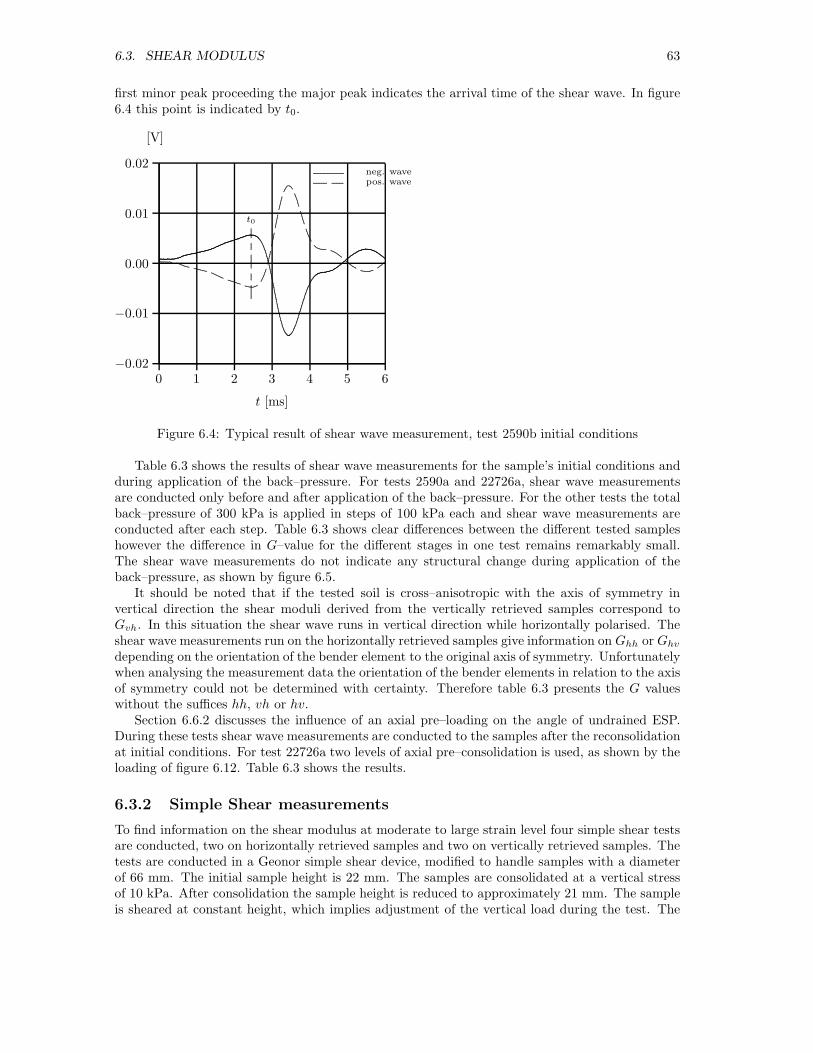
6.3. SHEAR MODULUS 63
first minor peak proceeding the major peak indicates the arrival time of the shear wave. In figure6.4 this point is indicated by t0.
0 1 2 3 4 5 6
t [ms]
−0.02
−0.01
0.00
0.01
0.02
[V]
.......................................................................................................................
............................................................................................
................................................................................................................
..............................................................
...........................................................................................................................................................................................................................................................................................................................................................................................................................................................................................................................
...........................................................................................................................................................................................................................................
.........................................................
.......................... .......................... .......................... .......................... .......................... ......................................................................................................................................................................................
..............................................................................
.......................... .................................................... ..........................
..................
.......................... ......................
.....
.....
.....
.....
.....
.
.....
.....
...
.....
.....
.....
.....
.....
.
.....
.....
...
.....
.....
.....
...
pos. waveneg. wave
t0
Figure 6.4: Typical result of shear wave measurement, test 2590b initial conditions
Table 6.3 shows the results of shear wave measurements for the sample’s initial conditions andduring application of the back–pressure. For tests 2590a and 22726a, shear wave measurementsare conducted only before and after application of the back–pressure. For the other tests the totalback–pressure of 300 kPa is applied in steps of 100 kPa each and shear wave measurements areconducted after each step. Table 6.3 shows clear differences between the different tested sampleshowever the difference in G–value for the different stages in one test remains remarkably small.The shear wave measurements do not indicate any structural change during application of theback–pressure, as shown by figure 6.5.
It should be noted that if the tested soil is cross–anisotropic with the axis of symmetry invertical direction the shear moduli derived from the vertically retrieved samples correspond toGvh. In this situation the shear wave runs in vertical direction while horizontally polarised. Theshear wave measurements run on the horizontally retrieved samples give information on Ghh or Ghvdepending on the orientation of the bender element to the original axis of symmetry. Unfortunatelywhen analysing the measurement data the orientation of the bender elements in relation to the axisof symmetry could not be determined with certainty. Therefore table 6.3 presents the G valueswithout the suffices hh, vh or hv.
Section 6.6.2 discusses the influence of an axial pre–loading on the angle of undrained ESP.During these tests shear wave measurements are conducted to the samples after the reconsolidationat initial conditions. For test 22726a two levels of axial pre–consolidation is used, as shown by theloading of figure 6.12. Table 6.3 shows the results.
6.3.2 Simple Shear measurements
To find information on the shear modulus at moderate to large strain level four simple shear testsare conducted, two on horizontally retrieved samples and two on vertically retrieved samples. Thetests are conducted in a Geonor simple shear device, modified to handle samples with a diameterof 66 mm. The initial sample height is 22 mm. The samples are consolidated at a vertical stressof 10 kPa. After consolidation the sample height is reduced to approximately 21 mm. The sampleis sheared at constant height, which implies adjustment of the vertical load during the test. The

64 CHAPTER 6. LABORATORY MEASUREMENTS
0 1 2 3 4 5
t [ms]
−0.01
0.00
0.01[V]
initial100 kPa back pressure200 kPa back pressure300 kPa back pressure
...........................................................................
.....................................................................................................................
.....................................................................
......................................................................................
...................................................................................................................................................................................................................................................................................................................................................................................
...................................................................................................................................................................................................................................
........................................................
.......................................................................
.......................... ..........................
.......................... ...................................................
. .......................... ..........................
..........................
..........................
..........................
..........................
..........................
....................................................
..........................
..........................
.......................... ..........................
..........................
.
.......................... ........... ....................
.......................... ..............................
....... ........... ..........................
........... .......................... .......
......................................... ..........................
...............................................................................................................
............................................................................................................... ...........
.......................... ............................
......... ...................
.......................... ........... ...........
..................................... ........... ........................
.. ........... ........... .......................... ........... ...........
.......................... ...........
..................................................................................................................................... .......
.................................................................................................... ...........
.......................... ...........
.....................................
.....
Figure 6.5: Development of the negative shear wave of test 1316a during raising of the back–pressure
Table 6.3: Results of shear wave measurementsvert. retrieved samples hor. retrieved samples
test 2590a 2590b 1316a 3963b 22726a 24482cG G G G G G
[kPa] [kPa] [kPa] [kPa] [kPa] [kPa]initial 635 865 960 1715 740 2010bp 100 kPa 930 970 1770 1208bp 200 kPa 860 960 1820 1170bp 300 kPa 665 895 950 1765 735 1170pre consol at 1135q = 30 kPapre consol. at 2335 2145 1450 3215q = 55 kPa
samples are sheared until the horizontal deformation equals 10 mm. The relevant parameters aregiven by:
∆γ =uhorha
, ∆τ =∆FhA
, G =∆τ
∆γ(6.9)
with:
uhor = horizontal deformationha = actual sample heightFh = horizontal forceA = sample surface
The maximum horizontal deformation of 10 mm corresponds to a maximum γ of 47 %. Themeasured shear stress, τ is corrected for the friction losses in the system and membrane.
To test the influence of an axial pre–consolidation one of the horizontally retrieved samplesand one of the vertically retrieved samples is axially pre–consolidated in the K0–CRS device. Thesamples are consolidated at an axial strain of 35 %. Figure 6.6 shows the results.
Figure 6.7 shows the development of the measured shear modulus versus the logarithm of theshear strain. The actual value for G is given by the slope of the tangent line of the τ - γ curve,

6.3. SHEAR MODULUS 65
0 10 20 30 40 50
γ [%]
−2
0
2
4
6
8
10
12
14
16
18
20τ [kPa]
........................................................................
.............
............
............................................................................................................................................................................................................................................................................................................................................................................................................................
.................................................................
...........................................................................
.........................................
..........................................
......................................................................................
........................................................................................................................
.............................................................................................................................................................
.........................................................................................................
.............................................................................................................................
................................................................................
.............................................................................................................................................
.......................... .......................... ..
.......
.....
......
.............................................................................................................
............................. .....
..................... .....................
...............................
.......................... .......................... ........
.................. .......................... .....................
..... .......................... .......................... .......................... ..........................
.......................... .......................... ..........................
.......................... .......................... ....................................................
.......................... ..........................
.......................... .......................... .
.....
.....
.....
.....
.....
.....
........
.......................... ...... ......................
.................
.........
.....
.
.....
.....
.....
.....
.....
.......................................................................................................................................
..........................................................
............................
..........
..........................
...... ..........................
...... .......................... ...... .............
............. ...... ................
.......... ...... .......................... ...... .......................... ...... .......................... ...... ................................ ..........................
...... .......................... ...... .......................... ................................ ...... .......................... ......
.......................................
.......................... ...... ...... .......
...................
.......
..................................................................................................................
......................................
.................................................. ..
.......................................................
....... ............
..........................
...... ................................
............ .......................... ......
...... .......................... ...... ...... .......................... ...... ...... .......................... ...... ...... .......................... ...... ......
.......................... ...... ...... ..........................
...... ................................ .....
vert. non pre–loaded
hor. non pre–loaded
vert. pre–loaded
hor. pre–loaded
Figure 6.6: Results of simple shear tests
figure 6.6. The G value presented in figure 6.7 is found by application of the least squares methodto each set of ten successive measurement data points. The angle of the fitted line represents theshear modulus and is depicted at the average γ for the ten regarded points.
10−6 10−5 10−4 10−3 10−2 0.1 1
γ [ - ]
−500
0
500
1000
1500
2000
2500
3000
3500
G [kPa]
•
◦
∗
⋄
1316b vert. non pre–loaded
22726b hor. non pre–loaded
22726c hor. pre–loaded
2590c vert. pre–loaded
av. Bender test pre–loaded
av. Bender test non pre–loaded
•••• •••••••••••••••••••••••••••••••••••••••••••••••••••••••••••••••••••••••••••••••••••••••••••••••••••••••••••••••••••••••••••••••••••••••••••••••••••••••••
•••••••••••••••••••••••••••••••••••••••••••••••••••••••••••••••••••••••••••••••••••••••••
•••••••••••••••••••••••••••••••••
◦
◦
◦◦◦
◦◦
◦◦◦◦◦◦◦◦◦◦◦◦◦◦◦ ◦◦
◦◦◦◦◦◦◦◦◦◦◦◦◦◦◦◦◦◦◦◦◦◦◦◦◦◦◦◦◦◦◦◦◦◦◦◦◦◦◦◦◦◦◦◦◦◦◦◦◦◦◦◦◦◦◦◦◦◦◦◦◦◦◦◦◦◦◦◦◦◦◦◦◦◦◦◦◦◦◦◦◦◦◦◦◦◦◦◦◦◦◦◦◦◦◦◦◦◦◦◦◦◦◦◦◦◦◦◦◦◦◦◦◦◦◦◦◦◦◦◦◦◦◦◦◦◦◦◦◦◦◦◦◦◦◦◦◦
◦◦◦◦◦◦◦◦◦◦◦◦◦◦◦◦◦◦◦◦◦◦◦◦◦◦◦◦◦◦◦◦◦◦◦◦◦◦◦◦◦◦◦◦◦◦◦◦◦◦◦◦◦◦◦◦◦◦◦◦◦◦◦◦◦◦◦◦◦◦◦◦◦◦◦◦◦◦◦◦◦◦◦◦◦◦◦◦◦◦◦◦◦◦◦◦◦◦◦◦◦◦◦◦◦◦◦◦◦◦◦◦◦◦◦◦◦◦◦◦◦◦◦◦◦◦◦◦◦◦◦◦◦◦◦◦◦◦◦◦◦◦◦◦◦◦◦◦◦◦◦◦◦◦◦◦◦◦◦◦◦◦◦◦◦◦◦◦◦◦◦◦◦◦◦◦◦◦◦◦◦◦
◦◦◦◦◦◦◦◦◦◦◦◦◦◦◦◦◦◦◦◦◦◦◦◦◦◦◦◦◦◦◦◦◦◦◦◦◦◦◦◦◦◦◦◦◦◦◦◦◦◦◦◦◦◦◦◦◦◦◦◦◦◦◦◦◦◦◦◦◦◦◦◦◦◦◦◦◦◦◦◦◦◦◦◦◦◦◦◦◦◦◦◦◦◦◦◦◦◦◦◦◦◦◦◦◦◦◦◦◦◦◦◦◦◦◦◦◦◦◦◦◦◦◦◦◦◦◦◦◦◦◦◦◦◦◦◦◦◦◦◦◦◦◦◦◦◦◦◦◦◦◦◦◦◦◦◦◦◦◦◦◦◦◦◦◦◦◦◦◦◦◦◦◦◦◦◦◦◦◦◦◦◦◦◦◦◦◦◦◦◦◦◦◦◦◦◦◦◦◦◦◦◦◦◦◦◦◦◦◦◦◦◦◦◦◦◦◦◦◦◦◦◦◦◦◦◦◦◦◦◦◦◦◦◦◦◦◦◦◦◦◦◦◦◦◦◦◦◦◦◦◦◦◦◦◦◦◦◦◦◦◦◦◦◦◦◦◦◦◦◦◦◦◦◦◦◦◦◦◦◦◦◦◦◦◦◦◦◦◦◦◦◦◦◦◦◦◦◦◦◦◦◦◦◦◦◦◦◦◦◦◦◦◦◦◦◦◦◦◦◦◦◦◦◦◦◦◦◦◦◦◦◦◦◦◦◦◦◦◦◦◦◦◦◦◦◦◦◦◦◦◦◦◦◦◦◦◦◦◦◦◦◦◦◦◦◦◦◦◦◦◦◦◦◦◦◦◦◦◦◦◦◦◦◦◦◦◦◦◦◦◦◦◦◦◦◦◦◦◦◦◦◦◦◦◦◦◦◦◦◦◦◦◦◦◦◦◦◦◦◦◦◦◦◦◦◦◦◦◦◦◦◦◦◦◦◦◦◦◦◦◦◦◦◦◦◦◦◦◦◦◦◦◦◦◦◦◦◦◦◦◦◦◦◦◦◦◦◦◦◦◦◦◦◦◦◦◦◦◦◦◦◦◦◦◦◦◦◦◦◦◦◦◦◦◦◦◦◦◦◦◦◦◦◦◦◦◦◦◦◦◦◦◦◦◦◦◦◦◦◦◦◦◦◦◦◦◦◦◦◦◦◦◦◦◦◦◦◦◦◦◦◦◦◦◦◦◦◦◦◦◦◦◦◦◦◦◦◦◦◦◦◦◦◦◦◦◦◦◦◦◦◦◦◦◦◦◦◦◦◦◦◦◦◦◦◦◦◦◦◦◦◦◦◦◦◦◦◦◦◦◦◦◦◦◦◦◦◦◦◦◦◦◦◦◦◦◦◦◦◦◦◦◦◦◦◦◦◦◦◦◦◦◦◦◦◦◦◦◦◦◦◦◦◦◦◦◦◦◦◦◦◦◦◦◦◦◦◦◦◦◦◦◦◦◦◦◦◦◦◦◦◦◦◦◦◦◦◦◦◦◦◦◦◦◦◦◦◦◦◦◦◦◦◦◦◦◦◦◦◦◦◦◦◦◦◦◦◦◦◦◦◦◦◦◦◦◦◦◦◦◦◦◦◦◦◦◦◦◦◦◦◦◦◦◦◦◦◦◦◦◦◦◦◦◦◦◦◦◦◦◦◦◦◦◦◦◦◦◦◦◦◦◦◦◦◦◦◦◦◦◦◦◦◦◦◦◦◦◦◦◦◦◦
∗
∗
∗∗∗∗
∗
∗
∗
∗∗∗
∗∗∗∗∗∗∗∗∗∗∗∗∗∗∗∗∗∗∗∗∗∗∗∗∗
∗∗∗∗∗∗∗∗∗∗∗∗∗∗∗∗∗∗∗∗∗∗∗∗∗∗∗∗∗∗∗∗∗∗∗∗∗∗∗∗∗∗∗∗∗∗∗∗∗∗∗∗∗∗∗∗∗∗∗∗∗∗∗∗∗∗∗∗∗∗∗∗∗∗∗∗∗∗∗∗∗∗∗∗∗∗∗∗∗∗∗∗∗∗∗∗∗∗∗∗∗∗∗∗∗∗∗∗∗∗∗∗∗∗∗∗∗∗∗∗∗∗∗∗∗∗∗∗∗∗∗∗∗∗∗∗∗∗∗∗∗∗∗∗∗∗∗∗∗∗∗∗∗∗∗∗∗∗∗∗∗∗∗∗∗∗∗∗∗∗∗∗∗∗∗∗∗∗∗∗∗∗∗∗∗∗∗∗∗∗∗∗∗∗∗∗∗∗∗∗∗∗∗∗∗∗∗∗∗∗∗∗∗∗∗∗∗∗∗∗∗∗∗∗∗∗∗∗∗∗∗∗∗∗∗∗∗∗∗∗∗∗∗∗∗∗∗∗∗∗∗∗∗∗∗∗∗∗∗∗∗∗∗∗∗∗∗∗∗∗∗∗∗∗∗∗∗∗∗∗∗∗∗∗∗∗∗∗∗∗∗∗∗∗∗∗∗∗∗∗∗∗∗∗∗∗∗∗∗∗∗∗∗∗∗∗∗∗∗∗∗∗∗∗∗∗∗∗∗∗∗∗∗∗∗∗∗∗∗∗∗∗∗∗∗∗∗∗∗∗∗∗∗∗∗∗∗∗∗∗∗∗∗∗∗∗∗∗∗∗∗∗∗∗∗∗∗∗∗∗∗∗∗∗∗∗∗∗∗∗∗∗∗∗∗∗∗∗∗∗∗∗∗∗∗∗∗∗∗∗∗∗∗∗∗∗∗∗∗∗∗∗∗∗∗∗∗∗∗∗∗∗∗∗∗∗∗∗∗∗∗∗∗∗∗∗∗∗∗∗∗∗∗∗∗∗∗∗∗∗∗∗∗∗∗∗∗∗∗∗∗∗∗∗∗∗∗∗∗∗∗∗∗∗∗∗∗∗∗∗∗∗∗∗∗∗∗∗∗∗∗∗∗∗∗∗∗∗∗∗∗∗∗∗∗∗∗∗∗∗∗∗∗∗∗∗∗∗∗∗∗∗∗∗∗∗∗∗∗∗∗∗∗∗∗∗∗∗∗∗∗∗∗∗∗∗∗∗∗∗∗∗∗∗∗∗∗∗∗∗∗∗∗∗∗∗∗∗∗∗∗∗∗∗∗∗∗∗∗∗∗∗∗∗∗∗∗∗∗∗∗∗∗∗∗∗∗∗∗∗∗∗∗∗∗∗∗∗∗∗∗∗∗∗∗∗∗∗∗∗∗∗∗∗∗∗∗∗∗∗∗∗∗∗∗∗∗∗∗∗∗∗∗∗∗∗∗∗∗∗∗∗∗∗∗∗∗∗∗∗∗∗∗∗∗∗∗∗∗∗∗∗∗∗∗∗∗∗∗∗∗∗∗∗∗∗∗∗∗∗∗∗∗∗∗∗∗∗∗∗∗∗∗∗∗∗∗∗∗∗∗∗∗∗∗∗∗∗∗∗∗∗∗∗∗∗∗∗∗∗∗∗∗∗∗∗∗∗∗∗∗∗∗∗∗∗∗∗∗∗∗∗∗∗∗∗∗∗∗∗∗∗∗∗∗∗∗∗∗∗∗∗∗∗∗∗∗∗∗∗∗∗∗∗∗∗∗∗∗∗∗∗∗∗∗∗∗∗∗∗∗∗∗∗∗∗∗∗∗∗∗∗∗∗∗∗∗∗
⋄⋄⋄⋄⋄
⋄⋄⋄⋄⋄⋄⋄⋄⋄⋄⋄⋄⋄⋄⋄⋄⋄⋄⋄⋄⋄⋄⋄⋄⋄⋄⋄⋄⋄⋄
⋄⋄⋄⋄⋄⋄⋄⋄⋄⋄⋄⋄⋄⋄⋄⋄⋄⋄⋄⋄⋄⋄⋄⋄⋄⋄⋄⋄⋄⋄⋄⋄⋄⋄⋄⋄⋄⋄⋄⋄⋄⋄⋄⋄⋄⋄⋄⋄⋄⋄⋄⋄⋄⋄⋄⋄⋄⋄⋄⋄⋄⋄⋄⋄⋄⋄⋄⋄⋄⋄⋄⋄⋄⋄⋄⋄⋄⋄⋄⋄⋄⋄⋄⋄⋄⋄⋄⋄⋄⋄⋄⋄⋄⋄⋄⋄⋄⋄⋄⋄⋄⋄⋄⋄⋄⋄⋄⋄⋄⋄⋄⋄⋄⋄⋄⋄⋄⋄⋄⋄⋄⋄⋄⋄⋄⋄⋄⋄⋄⋄⋄⋄⋄⋄⋄⋄⋄⋄⋄⋄⋄⋄⋄⋄⋄⋄⋄⋄⋄⋄⋄⋄⋄⋄⋄⋄
⋄⋄⋄⋄⋄⋄⋄⋄⋄⋄⋄⋄⋄⋄⋄⋄⋄⋄⋄⋄⋄⋄⋄⋄⋄⋄⋄⋄⋄⋄⋄⋄⋄⋄⋄⋄⋄⋄⋄⋄⋄⋄⋄⋄⋄⋄⋄⋄⋄⋄⋄⋄⋄⋄⋄⋄⋄⋄⋄⋄⋄⋄⋄⋄⋄⋄⋄⋄⋄⋄⋄⋄⋄⋄⋄⋄⋄⋄⋄⋄⋄⋄⋄⋄⋄⋄⋄⋄⋄⋄⋄⋄⋄⋄⋄⋄⋄⋄⋄⋄⋄⋄⋄⋄⋄⋄⋄⋄⋄⋄⋄⋄⋄⋄⋄⋄⋄⋄⋄⋄⋄⋄⋄⋄⋄⋄⋄⋄⋄⋄⋄⋄⋄⋄⋄⋄⋄⋄⋄⋄⋄⋄⋄⋄⋄⋄⋄⋄⋄⋄⋄⋄⋄⋄⋄⋄⋄⋄⋄⋄⋄⋄⋄⋄⋄⋄⋄⋄⋄⋄⋄⋄⋄⋄⋄⋄⋄⋄⋄
⋄⋄⋄⋄⋄⋄⋄⋄⋄⋄⋄⋄⋄⋄⋄⋄⋄⋄⋄⋄⋄⋄⋄⋄⋄⋄⋄⋄⋄⋄⋄⋄⋄⋄⋄⋄⋄⋄⋄⋄⋄⋄⋄⋄⋄⋄⋄⋄⋄⋄⋄⋄⋄⋄⋄⋄⋄⋄⋄⋄⋄⋄⋄⋄⋄⋄⋄⋄⋄⋄⋄⋄⋄⋄⋄⋄⋄⋄⋄⋄⋄⋄⋄⋄⋄⋄⋄⋄⋄⋄⋄⋄⋄⋄⋄⋄⋄⋄⋄⋄⋄⋄⋄⋄⋄⋄⋄⋄⋄⋄⋄⋄⋄⋄⋄⋄⋄⋄⋄⋄⋄⋄⋄⋄⋄⋄⋄⋄⋄⋄⋄⋄⋄⋄⋄⋄⋄⋄⋄⋄⋄⋄⋄⋄⋄⋄⋄⋄⋄⋄⋄⋄⋄⋄⋄⋄⋄⋄⋄⋄⋄⋄⋄⋄⋄⋄⋄⋄⋄⋄⋄⋄⋄⋄⋄⋄⋄⋄⋄⋄⋄⋄⋄⋄⋄⋄⋄⋄⋄⋄⋄⋄⋄⋄⋄⋄⋄⋄⋄⋄⋄⋄⋄⋄⋄⋄⋄⋄⋄⋄⋄⋄⋄⋄⋄⋄⋄⋄⋄⋄⋄⋄⋄⋄⋄⋄⋄⋄⋄⋄⋄⋄⋄⋄⋄⋄⋄⋄⋄⋄⋄⋄⋄⋄⋄⋄⋄⋄⋄⋄⋄⋄⋄⋄⋄⋄⋄⋄⋄⋄⋄⋄⋄⋄⋄⋄⋄⋄⋄⋄⋄⋄⋄⋄⋄⋄⋄⋄⋄⋄⋄⋄⋄⋄⋄⋄⋄⋄⋄⋄⋄⋄⋄⋄⋄⋄⋄⋄⋄⋄⋄⋄⋄⋄⋄⋄⋄⋄⋄⋄⋄⋄⋄⋄⋄⋄⋄⋄⋄⋄⋄⋄⋄⋄⋄⋄⋄⋄⋄⋄⋄⋄⋄⋄⋄⋄⋄⋄⋄⋄⋄⋄⋄⋄⋄⋄⋄⋄⋄⋄⋄⋄⋄⋄⋄⋄⋄⋄⋄⋄⋄⋄⋄⋄⋄⋄⋄⋄⋄⋄⋄⋄⋄⋄⋄⋄⋄⋄⋄⋄⋄⋄⋄⋄⋄⋄⋄⋄⋄⋄⋄⋄⋄⋄⋄⋄⋄⋄⋄⋄⋄⋄⋄⋄⋄⋄⋄⋄⋄⋄⋄⋄⋄⋄⋄⋄⋄⋄⋄⋄⋄⋄⋄⋄⋄⋄⋄⋄⋄⋄⋄⋄⋄⋄⋄⋄⋄⋄⋄⋄⋄⋄⋄⋄⋄⋄⋄⋄⋄⋄⋄⋄⋄⋄⋄⋄⋄⋄⋄⋄⋄⋄⋄⋄⋄⋄⋄⋄⋄⋄⋄⋄⋄⋄⋄⋄⋄⋄⋄⋄⋄⋄⋄⋄⋄⋄⋄⋄⋄⋄⋄⋄⋄⋄⋄⋄⋄⋄⋄⋄⋄⋄⋄⋄⋄⋄⋄⋄⋄⋄⋄⋄⋄⋄⋄⋄⋄⋄⋄⋄⋄⋄⋄⋄⋄⋄⋄⋄⋄⋄⋄⋄⋄⋄⋄⋄⋄⋄⋄⋄⋄⋄⋄⋄⋄⋄⋄⋄⋄⋄⋄⋄⋄⋄⋄⋄⋄⋄⋄⋄⋄⋄⋄⋄⋄⋄⋄⋄⋄⋄⋄⋄⋄⋄⋄⋄⋄⋄⋄⋄⋄⋄⋄⋄⋄⋄
......................................................
...........................................
.......................... ...................
.......................... ........
Figure 6.7: Simple Shear tests on pre–loaded and non pre–loaded samples
Figure 6.7 presents the results for fits with a relative least squares sum R2 > 0.8 (R2 = 1.0represents a perfect fit). Figure 6.6 shows a clearly non–monotone development of the τ–γ curve.The saw tooth shape of the curve can be explained by the presence of the fibres. At small strain

66 CHAPTER 6. LABORATORY MEASUREMENTS
level only a limited number of fits for which R2 > 0.8 can be shown. For γ < 5 × 10⁻⁴ onlyfor the both horizontally retrieved samples G values are plotted in figure 6.7. The differencesbetween horizontally and vertically retrieved samples are small and can be explained by naturalheterogeneity. The differences between the pre–loaded and non pre–loaded samples are clearer. Inthe range 10−3 < γ < 10−2 the G value for the pre–loaded samples is approximately twice thevalue for the non pre–loaded samples. For large strain the measured G converges. This is to beexpected since large strain is dominated by plasticity and the effects of a pre–loading vanishes.
At the left side of figure 6.7 the results of the bender element tests are presented. The Benderelement tests present the G–value at a very small strain level, Dyvik & Madshus [29] report a strainlevel of 10−5 for bender element tests. Extrapolation of the simple shear data to small strain levelshows that the simple shear data is in agreement with the bender element test results.
Keverling Buisman & Huizinga [46] propose a hyperbolic law to describe the τ–γ relation, whichis also elaborated by Kondner & Zelasko [48]. The proposed hyperbolic law is given by:
τ =γ
a+ bγ(6.10)
In which a and b are coefficients to be fitted by a curve fitting procedure. Using equation 6.10 anexpression for the shear modulus is found:
G =∂τ
∂γ=
a
(a+ bγ)2 , G0 =
1
a(6.11)
Table 6.4: Determination of G0 by curve fitting equation (6.10)test a b R2 G0
1316 non pre–loaded 0.0031 0.0848 0.99 32022726 non pre–loaded 0.0039 0.095 0.99 26022726 pre–loaded 0.0013 0.051 0.99 7902590 pre–loaded 0.0018 0.046 0.99 565
0.0 0.1 0.2 0.3 0.4 0.5
γ [ - ]
0.00
0.01
0.02
0.03
0.04
0.05
γ/τ [1/kPa]
2590c pl
22726c pl
22726b
1316b
••••••••••••••••••••••••••••••••••••••••••••••••••••••••••••••••••••••••••••••••••••••••••••••••••••••••••••••••••••••••••••••••••••••••••••••••••••••••••••••••••••••••••••••••••••••••••••••••••••••••••••••••••••••••••••••••••••••••••••••••••••••••••••••••••••••••••••••••••••••••••••••••••••••••••••••••••••••••••••••
•••••••••••••••••••••••••••••••••••
•••••••••••••••••••••••••••
••••••••••••••••••••••••
•••••••••••••••••••••••••••
••••••••••••••••••••
••••••••••••••••••••••••••••••••••••••••••••••••••••••
••••••••••••
◦◦◦◦◦◦◦◦◦◦◦◦◦◦◦◦◦◦◦◦◦◦◦◦◦◦◦◦◦◦◦◦◦◦◦◦◦◦◦◦◦◦◦◦◦◦◦◦◦◦◦◦◦◦◦◦◦◦◦◦◦◦◦◦◦◦◦◦◦◦◦◦◦◦◦◦◦◦◦◦◦◦◦◦◦◦◦◦◦◦◦◦◦◦◦◦◦◦◦◦◦◦◦◦◦◦◦◦◦◦◦◦◦◦◦◦◦◦◦◦◦◦◦◦◦◦◦◦◦◦◦◦◦◦◦◦◦◦◦◦◦◦◦◦◦◦◦◦◦◦◦◦◦◦◦◦◦◦◦◦◦◦◦◦◦◦◦◦◦◦◦◦◦◦◦◦◦◦◦◦◦◦◦◦◦◦◦◦◦◦◦◦◦◦◦◦◦◦◦◦◦◦◦◦◦◦◦◦◦◦◦◦◦◦◦◦◦◦◦◦◦◦◦◦◦◦◦◦◦◦◦◦◦◦◦◦◦◦◦◦◦◦◦◦◦◦◦◦◦◦◦◦◦◦◦◦◦◦◦◦◦◦◦◦◦◦◦◦◦◦◦◦◦◦◦◦◦◦◦◦◦◦◦◦◦◦◦◦◦◦◦◦◦◦◦◦◦◦◦◦◦◦◦◦◦◦◦◦◦◦◦◦◦◦◦◦◦◦◦◦◦◦◦◦◦◦◦◦◦◦◦◦◦◦◦◦◦◦◦◦◦◦◦◦◦◦◦◦◦◦◦◦◦◦◦◦◦◦◦◦◦◦◦◦◦◦◦◦◦◦◦◦◦◦◦◦◦◦◦◦◦◦◦◦◦◦◦◦◦◦◦◦◦◦◦◦◦◦◦◦◦◦◦◦◦◦◦◦◦◦◦◦◦◦◦◦◦◦◦◦◦◦◦◦◦◦◦◦◦◦◦◦◦◦◦◦◦◦◦◦◦◦◦◦◦◦◦◦◦◦◦◦◦◦◦◦◦◦◦◦◦◦◦◦◦◦◦◦◦◦◦◦◦◦◦◦◦◦◦◦◦◦◦◦◦◦◦◦◦◦◦◦◦◦◦◦◦◦◦◦◦◦◦◦◦◦◦◦◦◦◦◦◦◦◦◦◦◦◦◦◦◦◦◦◦◦◦◦◦◦◦◦◦◦◦◦◦◦◦◦◦◦◦◦◦◦◦◦◦◦◦◦◦◦◦◦◦◦◦◦◦◦◦◦◦◦◦◦◦◦◦◦◦◦◦◦◦◦◦◦◦◦◦◦◦◦◦◦◦◦◦◦◦◦◦◦◦◦◦◦◦◦◦◦◦◦◦◦◦◦◦◦◦◦◦◦◦◦◦◦◦◦◦◦◦◦◦◦◦◦◦◦◦◦◦◦◦◦◦◦◦◦◦◦◦◦◦◦◦◦◦◦◦◦◦◦◦◦◦◦◦◦◦◦◦◦◦◦◦◦◦◦◦◦◦◦◦◦◦◦◦◦◦◦◦◦◦◦◦◦◦◦◦◦◦◦◦◦◦◦◦◦◦◦◦◦◦◦◦◦◦◦◦◦◦◦◦◦◦◦◦◦◦◦◦◦◦◦◦◦◦◦◦◦◦◦◦◦◦◦◦◦◦◦◦◦◦◦◦◦◦◦◦◦◦◦◦◦◦◦◦◦◦◦◦◦◦◦◦◦◦◦◦◦◦◦◦◦◦◦◦◦◦◦◦◦◦◦◦◦◦◦◦◦◦◦◦◦◦◦◦◦◦◦◦◦◦◦◦◦◦◦◦◦◦◦◦◦◦◦◦◦◦◦◦◦◦◦◦◦◦◦◦◦◦◦◦◦
◦◦◦◦◦◦◦◦◦◦◦◦◦◦◦◦◦◦◦◦◦◦◦◦◦◦◦◦◦◦◦◦◦◦◦◦◦◦◦◦◦◦◦◦◦◦◦◦◦◦◦◦◦◦◦◦◦◦◦◦◦◦◦◦◦◦◦◦◦◦◦◦◦◦◦◦◦◦◦◦◦◦◦◦◦◦◦◦◦◦◦◦◦◦◦◦◦◦◦◦◦◦◦◦◦◦◦◦◦◦◦◦◦◦◦◦◦◦◦◦◦◦◦◦◦◦◦◦◦◦◦◦◦◦◦◦◦◦◦◦◦◦◦◦◦◦◦◦◦◦◦◦◦◦◦◦◦◦◦◦◦◦◦◦◦◦◦◦◦◦◦◦◦◦◦◦◦◦◦◦◦◦◦◦◦◦◦◦◦◦◦◦◦◦◦◦◦◦◦◦◦◦◦◦◦◦◦◦◦◦◦◦◦◦◦◦◦◦◦◦◦◦◦◦◦◦◦◦◦◦◦◦◦◦◦◦◦◦◦◦◦◦◦◦◦◦◦◦◦◦◦◦◦◦◦◦◦◦◦◦◦◦◦◦◦◦◦◦◦◦◦◦◦◦◦◦◦◦◦◦◦◦◦◦◦◦◦◦◦◦◦◦◦◦◦◦◦◦◦◦◦◦◦◦◦◦◦◦◦◦◦◦◦◦◦◦◦◦◦◦◦◦◦◦◦◦◦◦◦◦◦◦◦◦◦◦◦◦◦◦◦◦◦◦◦◦◦◦◦◦◦◦◦◦◦◦◦◦◦◦◦◦◦◦◦◦◦◦◦◦◦◦◦◦◦◦◦◦◦◦◦◦◦◦◦◦◦◦◦◦◦◦◦◦◦◦◦◦◦◦◦◦◦◦◦◦◦◦◦◦◦◦◦◦◦◦◦◦◦◦◦◦◦◦◦◦◦◦◦◦◦◦◦◦◦◦◦◦◦◦◦◦◦◦◦◦◦◦◦◦◦◦◦◦◦◦◦◦◦◦◦◦◦◦◦◦◦◦◦◦◦◦◦◦◦◦◦◦◦◦◦◦◦◦◦◦◦◦◦◦◦◦◦◦◦◦◦◦◦◦◦◦◦◦
◦◦◦◦◦◦◦◦◦◦◦◦◦◦◦◦◦◦◦◦◦◦◦◦◦◦◦◦◦◦◦◦◦◦◦◦◦◦◦◦◦◦◦◦◦◦◦◦◦◦◦◦◦◦◦◦◦◦◦◦◦◦◦◦◦◦◦◦◦◦◦◦◦◦◦◦◦◦◦◦◦◦◦◦◦◦◦◦◦◦◦◦◦◦◦◦◦◦◦◦◦◦◦◦◦◦◦◦◦◦◦◦◦◦◦◦◦◦◦◦◦◦◦◦◦◦◦◦◦◦◦◦◦◦◦◦◦◦◦◦◦◦◦◦◦◦◦◦◦◦◦◦◦◦◦◦◦◦◦◦◦◦◦◦◦◦◦◦◦◦◦◦◦◦◦◦◦◦◦◦◦
◦◦◦◦◦◦◦◦◦◦◦◦◦◦◦◦◦◦◦◦◦◦◦◦◦◦◦◦◦◦◦◦◦◦◦◦◦◦◦◦◦◦◦◦◦◦◦◦◦◦◦◦◦◦◦◦◦◦◦◦◦◦◦◦◦◦◦◦◦◦◦◦◦◦◦◦◦◦◦◦◦◦◦◦◦◦◦◦◦◦◦◦◦◦◦◦◦◦◦◦◦◦◦◦◦◦◦◦◦◦◦◦◦◦◦◦◦◦◦◦◦◦◦◦◦◦◦◦◦◦◦◦◦◦◦◦◦◦◦◦◦◦◦◦◦◦◦◦◦◦◦◦◦◦◦◦◦◦◦◦◦◦◦◦◦◦◦◦◦◦◦◦◦◦◦
◦◦◦◦◦◦◦◦◦◦◦◦◦◦◦◦◦◦◦◦◦◦◦◦◦◦◦◦◦◦◦◦◦◦◦◦◦◦◦◦◦◦◦◦◦◦◦◦◦◦◦◦◦◦◦◦◦◦◦◦◦◦◦◦◦◦◦◦◦◦◦◦◦◦◦◦◦◦◦◦◦◦◦◦◦◦◦◦◦◦◦◦◦◦◦◦◦◦◦◦◦◦◦◦◦◦◦◦◦◦◦◦◦◦◦◦◦◦◦◦◦◦◦◦◦◦◦◦◦◦◦◦◦◦◦◦◦◦◦◦◦◦◦◦◦◦
◦◦◦◦◦◦◦◦◦◦◦◦
∗∗∗∗∗∗∗∗∗∗∗∗∗∗∗∗∗∗∗∗∗∗∗∗∗∗∗∗∗∗∗∗∗∗∗∗∗∗∗∗∗∗∗∗∗∗∗∗∗∗∗∗∗∗∗∗∗∗∗∗∗∗∗∗∗∗∗∗∗∗∗∗∗∗∗∗∗∗∗∗∗∗∗∗∗∗∗∗∗∗∗∗∗∗∗∗∗∗∗∗∗∗∗∗∗∗∗∗∗∗∗∗∗∗∗∗∗∗∗∗∗∗∗∗∗∗∗∗∗∗∗∗∗∗∗∗∗∗∗∗∗∗∗∗∗∗∗∗∗∗∗∗∗∗∗∗∗∗∗∗∗∗∗∗∗∗∗∗∗∗∗∗∗∗∗∗∗∗∗∗∗∗∗∗∗∗∗∗∗∗∗∗∗∗∗∗∗∗∗∗∗∗∗∗∗∗∗∗∗∗∗∗∗∗∗∗∗∗∗∗∗∗∗∗∗∗∗∗∗∗∗∗∗∗∗∗∗∗∗∗∗∗∗∗∗∗∗∗∗∗∗∗∗∗∗∗∗∗∗∗∗∗∗∗∗∗∗∗∗∗∗∗∗∗
∗∗∗∗∗∗∗∗∗∗∗∗∗∗∗∗∗∗∗∗∗∗∗∗∗∗∗∗∗∗∗∗∗∗∗∗∗∗∗∗∗∗∗∗∗∗∗∗∗∗∗∗∗∗∗∗∗∗∗∗∗∗∗∗∗∗∗∗∗∗∗∗∗∗∗∗∗∗∗∗∗∗∗∗∗∗∗∗∗∗∗∗∗∗∗∗∗∗∗∗∗∗∗∗∗∗∗∗∗∗∗∗∗∗∗∗∗∗∗∗∗∗∗∗∗∗∗∗∗∗∗∗∗∗∗∗∗∗∗∗∗∗∗∗∗∗∗∗∗∗∗∗∗∗∗∗∗∗∗∗∗∗∗∗∗∗∗∗∗∗∗∗∗∗∗∗∗∗∗∗∗∗∗∗∗∗∗∗∗∗∗∗∗∗∗∗∗∗∗∗∗∗∗∗∗∗∗∗∗∗∗∗∗∗∗
∗∗∗∗∗∗∗∗∗∗∗∗∗∗∗∗∗∗∗∗∗∗∗∗∗∗∗∗∗∗∗∗∗∗∗∗∗∗∗∗∗∗∗∗∗∗∗∗∗∗∗∗∗∗∗∗∗∗∗∗∗∗∗∗∗∗∗∗∗∗∗∗∗∗∗∗∗∗∗∗∗∗∗∗∗∗∗∗∗∗∗∗∗∗∗∗∗∗∗∗∗∗∗∗∗∗∗∗∗∗∗∗∗∗∗∗∗∗∗∗∗∗∗∗∗∗∗∗∗∗∗∗∗∗∗∗∗∗∗∗∗∗∗∗∗∗∗∗∗∗∗∗∗∗∗∗∗∗∗∗∗∗∗∗∗∗∗∗∗∗∗∗∗∗∗∗∗∗∗∗∗∗∗∗∗∗∗∗∗∗∗∗∗∗∗∗∗∗∗∗∗∗∗∗∗∗∗∗∗∗∗∗∗∗∗∗∗∗∗∗∗∗∗∗∗∗∗∗∗
∗∗∗∗∗∗∗∗∗∗∗∗∗∗∗∗∗∗∗∗∗∗∗∗∗∗∗∗∗∗∗∗∗∗∗∗∗∗∗∗∗∗∗∗∗∗∗∗∗∗∗∗∗∗∗∗∗∗∗∗∗∗∗∗∗∗∗∗∗∗∗∗∗∗∗∗∗∗∗∗∗∗∗∗∗∗∗∗∗∗∗∗∗∗∗∗∗∗∗∗∗∗∗∗∗∗∗∗∗∗∗∗∗∗∗∗∗∗∗∗∗∗∗∗∗∗∗∗∗∗∗∗∗∗∗∗∗∗∗∗∗∗∗∗∗∗∗∗∗∗∗∗∗∗∗∗∗∗∗∗∗∗∗∗∗∗∗∗∗∗∗∗∗∗∗∗∗∗∗∗∗∗
∗∗∗∗∗∗∗∗∗∗∗∗∗∗∗∗∗∗∗∗∗∗∗∗∗∗∗∗∗∗∗∗∗∗∗∗∗∗∗∗∗∗∗∗∗∗∗∗∗∗∗∗∗∗∗∗∗∗∗∗∗∗∗∗∗∗∗∗∗∗∗∗∗∗∗∗∗∗∗∗∗∗∗∗∗∗∗∗∗∗∗∗∗∗∗∗∗∗∗∗∗∗∗∗∗∗∗∗∗∗∗∗∗∗∗∗∗∗∗∗∗∗∗∗∗∗∗∗∗∗∗∗∗∗∗∗∗∗∗∗∗
∗∗∗∗∗∗∗∗∗∗∗∗∗∗∗∗∗∗∗∗∗∗∗∗∗∗∗∗∗∗∗∗∗∗∗∗∗∗∗∗∗∗∗∗∗∗∗∗∗∗∗∗∗∗∗∗∗∗∗∗∗∗∗∗∗∗∗∗∗∗∗∗∗∗∗∗∗∗∗∗∗∗∗∗∗∗∗∗∗∗∗∗∗∗∗∗∗∗∗∗∗∗∗∗∗∗∗∗∗∗∗∗∗∗∗∗∗∗
∗∗∗∗∗∗∗∗∗∗∗∗∗∗∗∗∗∗∗∗∗∗∗∗∗∗∗∗∗∗∗∗∗∗∗∗∗∗∗∗∗∗∗∗∗∗∗∗∗∗∗∗∗∗∗∗∗∗∗∗∗∗∗∗∗∗∗∗∗∗∗∗∗∗∗∗∗∗∗∗∗∗∗∗∗∗∗∗∗∗∗∗∗∗∗∗∗∗∗∗∗∗∗∗∗∗∗∗∗∗∗∗∗∗∗∗∗∗∗∗∗∗∗∗∗∗∗∗∗∗∗∗∗∗∗∗∗∗∗∗∗∗∗∗∗∗∗∗∗∗∗∗∗∗∗∗∗∗∗∗∗∗∗∗∗∗∗∗∗
∗∗∗∗∗∗∗∗∗∗∗∗∗∗∗∗∗∗∗∗∗∗∗∗∗∗∗∗∗∗∗∗∗∗∗∗∗∗∗∗∗∗∗∗∗∗∗∗∗∗∗∗∗∗∗∗∗∗∗∗∗∗∗∗∗∗∗∗∗∗∗∗∗∗∗∗∗∗∗∗∗∗∗∗∗∗∗∗∗∗∗∗∗∗∗∗∗∗∗∗∗∗∗∗∗∗∗∗∗∗∗∗∗∗∗∗∗∗∗∗∗∗∗∗∗∗∗∗∗∗∗∗∗∗∗∗∗∗∗∗∗∗∗∗∗∗∗∗∗∗∗∗∗∗∗∗∗∗∗∗∗∗∗∗
⋄⋄⋄⋄⋄⋄⋄⋄⋄⋄⋄⋄⋄⋄⋄⋄⋄⋄⋄⋄⋄⋄⋄⋄⋄⋄⋄⋄⋄⋄⋄⋄⋄⋄⋄⋄⋄⋄⋄⋄⋄⋄⋄⋄⋄⋄⋄⋄⋄⋄⋄⋄⋄⋄⋄⋄⋄⋄⋄⋄⋄⋄⋄⋄⋄⋄⋄⋄⋄⋄⋄⋄⋄⋄⋄⋄⋄⋄⋄⋄⋄⋄⋄⋄⋄⋄⋄⋄⋄⋄⋄⋄⋄⋄⋄⋄⋄⋄⋄⋄⋄⋄⋄⋄⋄⋄⋄⋄⋄⋄⋄⋄⋄⋄⋄⋄⋄⋄⋄⋄⋄⋄⋄⋄⋄⋄⋄⋄⋄⋄⋄⋄⋄⋄⋄⋄⋄⋄⋄⋄⋄⋄⋄⋄⋄⋄⋄⋄⋄⋄⋄⋄⋄⋄⋄⋄⋄⋄⋄⋄⋄⋄⋄⋄⋄⋄⋄⋄⋄⋄⋄⋄⋄⋄⋄⋄⋄⋄⋄⋄⋄⋄⋄⋄⋄⋄⋄⋄⋄⋄⋄⋄⋄⋄⋄⋄⋄⋄⋄⋄⋄⋄⋄⋄⋄⋄⋄⋄⋄⋄⋄⋄⋄⋄⋄⋄⋄⋄⋄⋄⋄⋄⋄⋄⋄⋄⋄⋄⋄⋄⋄⋄⋄⋄⋄⋄⋄⋄⋄⋄⋄⋄⋄⋄⋄⋄⋄⋄⋄⋄⋄⋄⋄⋄⋄⋄⋄⋄⋄⋄⋄⋄⋄⋄⋄⋄⋄⋄⋄⋄⋄⋄⋄⋄⋄⋄⋄⋄⋄⋄⋄⋄⋄⋄⋄⋄⋄⋄⋄⋄⋄⋄⋄⋄⋄⋄⋄⋄⋄⋄⋄⋄⋄⋄⋄⋄⋄⋄⋄⋄⋄⋄⋄⋄⋄⋄⋄⋄⋄⋄⋄⋄⋄⋄⋄⋄⋄⋄⋄
⋄⋄⋄⋄⋄⋄⋄⋄⋄⋄⋄⋄⋄⋄⋄⋄⋄⋄⋄⋄⋄⋄⋄⋄⋄⋄⋄⋄⋄⋄⋄⋄⋄⋄⋄⋄⋄⋄⋄⋄⋄⋄⋄⋄⋄⋄⋄⋄⋄⋄⋄⋄⋄⋄⋄⋄⋄⋄⋄⋄⋄⋄⋄⋄⋄⋄⋄⋄⋄⋄⋄⋄⋄⋄⋄⋄⋄⋄⋄⋄⋄⋄⋄⋄⋄⋄⋄⋄⋄⋄⋄⋄⋄⋄⋄⋄⋄⋄⋄⋄⋄⋄⋄⋄⋄⋄⋄⋄⋄⋄⋄⋄⋄⋄⋄⋄⋄⋄⋄⋄⋄⋄⋄⋄⋄⋄⋄⋄⋄⋄⋄⋄⋄⋄⋄⋄⋄⋄⋄⋄⋄⋄⋄⋄⋄⋄⋄⋄⋄⋄⋄⋄⋄⋄⋄⋄⋄⋄⋄⋄⋄⋄⋄⋄⋄⋄⋄⋄⋄⋄⋄⋄⋄⋄⋄⋄⋄⋄⋄⋄⋄⋄⋄⋄⋄⋄⋄⋄⋄⋄⋄⋄⋄⋄⋄⋄⋄⋄⋄⋄⋄⋄⋄⋄⋄⋄⋄⋄⋄⋄⋄⋄⋄⋄⋄⋄⋄⋄⋄⋄⋄⋄⋄⋄⋄⋄⋄⋄⋄⋄⋄⋄⋄⋄⋄⋄⋄⋄⋄⋄⋄⋄⋄⋄⋄⋄⋄⋄⋄⋄⋄⋄⋄⋄⋄⋄⋄⋄⋄⋄⋄⋄⋄⋄⋄⋄⋄⋄⋄⋄⋄⋄⋄⋄⋄⋄⋄⋄⋄⋄⋄⋄⋄⋄⋄⋄⋄⋄⋄⋄⋄⋄⋄⋄⋄⋄⋄⋄⋄⋄⋄⋄⋄⋄⋄⋄⋄⋄⋄⋄⋄⋄⋄⋄⋄⋄⋄⋄⋄⋄⋄⋄⋄⋄⋄⋄⋄⋄⋄⋄⋄⋄⋄⋄⋄⋄⋄⋄⋄⋄⋄⋄⋄⋄⋄⋄⋄⋄⋄⋄⋄⋄⋄⋄⋄⋄⋄⋄⋄⋄⋄⋄⋄⋄⋄⋄⋄⋄⋄⋄⋄⋄⋄⋄⋄⋄⋄⋄⋄⋄⋄⋄⋄⋄
⋄⋄⋄⋄⋄⋄⋄⋄⋄⋄⋄⋄⋄⋄⋄⋄⋄⋄⋄⋄⋄⋄⋄⋄⋄⋄⋄⋄⋄⋄⋄⋄⋄⋄⋄⋄⋄⋄⋄⋄⋄⋄⋄⋄⋄⋄⋄⋄⋄⋄⋄⋄⋄⋄⋄⋄⋄⋄⋄⋄⋄⋄⋄⋄⋄⋄⋄⋄⋄⋄⋄⋄⋄⋄⋄⋄⋄⋄⋄⋄⋄⋄⋄⋄⋄⋄⋄⋄⋄⋄⋄⋄⋄⋄⋄⋄⋄⋄⋄⋄⋄⋄⋄⋄⋄⋄⋄⋄⋄⋄⋄⋄⋄⋄⋄⋄⋄⋄⋄⋄⋄⋄
⋄⋄⋄⋄⋄⋄⋄⋄⋄⋄⋄⋄⋄⋄⋄⋄⋄⋄⋄⋄⋄⋄⋄⋄⋄⋄⋄⋄⋄⋄⋄⋄⋄⋄⋄⋄⋄⋄⋄⋄⋄⋄⋄⋄⋄⋄⋄⋄⋄⋄⋄⋄⋄⋄⋄⋄⋄⋄⋄⋄⋄⋄⋄⋄⋄⋄⋄⋄⋄⋄⋄⋄⋄⋄⋄⋄⋄⋄⋄⋄⋄⋄⋄⋄⋄⋄⋄⋄⋄⋄⋄⋄⋄⋄⋄⋄⋄⋄⋄⋄⋄
⋄⋄⋄⋄⋄⋄⋄⋄⋄⋄⋄⋄⋄⋄⋄⋄⋄⋄⋄⋄⋄⋄⋄⋄⋄⋄⋄⋄⋄⋄⋄⋄⋄⋄⋄⋄⋄⋄⋄⋄⋄⋄⋄⋄⋄⋄⋄⋄⋄⋄⋄⋄⋄⋄⋄⋄⋄⋄⋄⋄⋄⋄⋄⋄⋄⋄⋄⋄⋄⋄⋄⋄⋄⋄⋄⋄⋄⋄⋄⋄⋄⋄⋄⋄⋄⋄⋄⋄⋄
⋄⋄⋄⋄⋄⋄⋄⋄⋄⋄⋄⋄⋄⋄⋄⋄⋄⋄⋄⋄⋄⋄⋄⋄⋄⋄⋄⋄⋄⋄⋄⋄⋄⋄⋄⋄⋄⋄⋄⋄⋄⋄⋄⋄⋄⋄⋄⋄⋄⋄⋄⋄⋄⋄⋄⋄⋄⋄⋄⋄⋄⋄⋄⋄⋄⋄⋄⋄⋄⋄⋄⋄⋄⋄⋄⋄⋄⋄⋄⋄⋄⋄⋄⋄⋄⋄⋄⋄⋄
⋄⋄⋄⋄⋄⋄⋄⋄⋄⋄⋄⋄⋄⋄⋄⋄⋄⋄⋄⋄⋄⋄⋄⋄⋄⋄⋄⋄⋄⋄⋄⋄⋄⋄⋄⋄⋄⋄⋄⋄⋄⋄⋄⋄⋄⋄⋄⋄⋄⋄⋄⋄⋄⋄⋄⋄⋄⋄⋄⋄⋄⋄⋄⋄⋄⋄⋄⋄⋄⋄⋄⋄⋄⋄⋄⋄⋄
⋄⋄⋄⋄⋄⋄⋄⋄⋄⋄⋄⋄⋄⋄⋄⋄⋄⋄⋄⋄⋄⋄⋄⋄
10−4 10−3 10−2 0.1 1
γ [ - ]
0
200
400
600
800G [kPa]
............................................................................................................................................................................................................................................................................................................................................................................................
.......................................................................................................................................................................................................................................................................................................................................................................................
........................................................................................................................................................................................................................................................................................................................................................................................................................................................................
..............................................................................................................................................................................................................................................................................................................................................................................................................................
2590c pl
22726c pl
22726b
1316b
Figure 6.8: Curve fitting for hyperbola law, following Kondner [48], pl = pre–loaded
Table 6.4 shows that the measurement data fit well to a hyperbolic law, with R2 close to 1.0.The table shows a clear difference in G0 for the pre–loaded and non pre–loaded samples. The valuesfor G0 found given by table 6.4 are considerably lower than found by the shear wave measurements.Using equation (6.11) a continuous G − γ curve can be found using the coefficients of table 6.4.Figure 6.8 shows the continuous G − γ development. Graph 6.7 shows a lower G0 than found bythe shear wave measurements and indicated by figure 6.7. From γ = 5 × 10⁻³ figure 6.7 and 6.8are in reasonable agreement.

6.4. PORE PRESSURE MEASUREMENT AT THE SAMPLE CENTRE 67
6.3.3 Conclusions
At the beginning of this section three reasons were mentioned for conducting shear wave measure-ments. The first reason is to derive information on the shear modulus, which can not be found bystandard triaxial testing. The results are presented in table 6.3. The bender element tests as wellas the Simple Shear tests do not show a clear difference between the horizontally and verticallyretrieved samples. The differences found can be explained by natural heterogeneity.
The second reason is to identify possible structural changes during application of the back–pressure. Figure 6.5 shows that the shear wave measurements remain unaffected by the back–pressure. Indications for a change in structure are not found.
The third reason is to check if the typical stress–strain development depicted by figure 6.3 alsoholds for peat and if a threshold value γ0 can be found. Figure 6.7 and 6.8 show a stiffness–straindevelopment that corresponds to the theoretical development given by figure 6.3. The shear wavemeasurement can be regarded as initial stiffness G0. Figure 6.7 shows that a plateau, a constantvalue for G could not be distinguished from measurements when looking at the slope of the tangentline for the τ − γ curve. In figure 6.8 such a plateau can be distinguished. However at small strainlevel the G values presented in figure 6.8 do not correspond to shear wave measurements. Fittingto a hyperbola seems to underestimate G0 significantly. Flattening of the curve at small strainlevel as predicted by figure 6.8 does not correspond to the shear wave measurements. It can beconcluded that the threshold value for γ0 can not be distinguished from measurements. If such athreshold value exists it falls beyond measurement accuracy of the Simple Shear device. So evenat small strain level a non–linear G should be accounted for.
6.4 Pore pressure measurement at the sample centre
.................................................................................................................................................................................................................
.....
...................................................................................................................................................
..................
.....................................................................................................................................................................................................................................................................................................................................................................................................................................................................................................................................................................................
........................................................................................................................................................
.....
.....
.....
.....
.....
.....
.....
.....
.....
.....
.....
.....
.....
................................................................................................................................................
..................
.....
.....
.....
.....
.....
.....
.....
.....
.....
.....
.....
.....
.....
.....
.....
.....
.....
.....
.....
.....
.....
.....
.....
.....
.....
.....
.....
.....
.....
.....
.....
.....
.....
.....
.....
.....
.....
.....
.....
.....
.....
.....
.....
.....
.....
.....
.....
.....
.....
.....
.....
.....
.....
.....
.....
.....
.....
.....
.....
.....
.....
.....
.....
.....
.....
.....
.....
.....
..
.....
.....
.....
.....
.....
.....
.....
.....
.....
.....
.....
.....
.....
.....
.....
.....
.....
.....
.....
.....
.....
.....
.....
.....
.....
.....
.....
.....
.....
.....
.....
.....
.....
.....
.....
.....
.....
.....
.....
.....
.....
.....
.....
.....
.....
.....
.....
.....
.....
.....
.....
.....
.....
.....
.....
.....
.....
.....
.....
.....
.....
.....
.....
.....
.....
.....
.....
.....
.....
.....
.....
.....
.....
.....
.....
.....
.....
..
...........................
...........................
....................................
....................................
..........................................................................................................................................................................................................................................................................................................................
................
................
................
................
................
................
.............................................................................................. .............................................................. ...................
upper drain
....................................................................................................................................................................................... .............................................................. ...................
lower drain
sample
pore pressure transducerneedle
top cap
footingporous stone
porous stone
membrane
drain.......................................................
...................
........................................................................................................................................................................................................................................................ ................... to external p.p. transducer
.........
.........
.........
.........
.........
.........
.........
.........
.........
.........
.........
.........
.........
.........
.........
.........
.........
.........
.........
.........
.........
.........
.........
.........
.........
.........
.........
.........
.........
.........
.........
.........
.........
.........
.........
.........
.........
.........
.........
.........
.........
.........
.........
.........
.........
.........
.........
.........
.........
Figure 6.9: Test set-up
To generate the Mandel–Cryer effect in atriaxial test a radial pore water flow isneeded. To create a radial pore water flowpaper drains are placed between the sampleand the membrane. At top and bottom astiff impermeable plate is placed. This plateprevents direct pore water dissipation fromthe sample to the porous stone. The pa-per drains are extended beyond the plate attop and bottom and are connected to theporous stones. At the centre of the foot-ing a connection is made between the sam-ple and a pore pressure transducer. Thistransducer is referred to as the externallyplaced transducer. The expelled pore wateris collected in the chambers of the hydraulicpiston controlling the back–pressure. Ne-glecting pressure losses in the tubes betweentriaxial cell and piston, the actual pressurein the hydraulic piston equals the pressurein the drainage system, paper drains and
porous stones. Figure 6.9 sketches the test set–up.The Mandel–Cryer effect is only found at the centre of the sample. So pore pressure measure-
ments inside the sample are needed. Figure 6.10b shows a miniature pore pressure transducer thatis connected to a needle. When preparing the sample the needle is pierced through the membrane.The length of the needle is 3 cm. So when placed carefully the tip of the needle reaches the centreof the sample. Some glue is used to connect the needle firmly to the membrane. Application of the

68 CHAPTER 6. LABORATORY MEASUREMENTS
glue also prevents possible leakage of pore water along the needle through the membrane. Figure6.10a shows the needle placed inside a sample. The casing connecting the end of the needle to thepore pressure transducer contains a porous stone to protect the transducer. Complete saturationof the porous stone is achieved by placing the stone, transducer and needle in a cup of waterthat is placed in an exicator in which a vacuum is applied for one hour. Saturation of the casingand the needle was easily achieved by flushing both with de–aired water. The saturation of theporous stone, needle and casing was regularly checked by comparing measurements of the needleand external transducer.
Figure 6.10: a) Test facility, b) Needle, casing and pore pressure transducer
The analytical solutions presented in chapter 5 assume deformations to be uniformly distributedin axial direction. In order to meet this assumption shear stress along the top cap and footing ofthe sample should be minimised. Therefore a membrane is placed between the sample and top caprespectively footing. Silicone grease is used to reduce further friction.
6.5 Initial saturation, B–factor measurement
Chapter 2 shows the influence of gas bubbles on the compressibility of the pore fluid. Even a smallamount of gas raises the pore fluid compressibility considerably. The mathematical descriptionpresented in chapter 5 assumes an incompressible pore fluid. In practice this condition is reachedwhen the compressibility of the skeleton exceeds the compressibility of the pore fluid in an orderof magnitude. This is illustrated by equation (4.40). Equation (4.40) also illustrates the influenceof the Skempton B–factor on the measurement results. When the B–factor is not well controlleda reduced pore pressure is measured. It is therefore important to check the degree of saturationbefore comparing experimental results to theory.
Chapter 2 introduces the Skempton B–factor which is further discussed in chapter 4. Equation(2.17) shows the Skempton B–factor to be some function of the compressibility of pore fluid, solidsand skeleton. For clay and sand the solids can be considered as incompressible. The SkemptonB–factor reduces to a function of pore fluid and skeleton compressibility. Therefore, in standardtriaxial testing B–factor measurement is usually conducted to check the saturation of the sample.
Since peat has an organic nature, fibres could conceivably contain air pockets. If such an air

6.5. INITIAL SATURATION, B–FACTOR MEASUREMENT 69
pocket is not in contact with the pores a fibre with such an air pocket can be seen as a compressiblesolid. The Skempton B–factor is then a function of the compressibility of solids, pore fluid andskeleton. If the solids of peat can be considered as compressible B–factor measurement is notenough to check the saturation of the sample. A possible low degree of saturation leading to a lowB–factor might be masked by the compressibility of the solids leading to a B–factor increase. Tocheck if compressibility of the solids influences pore pressure development Sri and B–factor arecalculated under the assumption of incompressible solids, using equation (2.16). If the measuredB–factor corresponds to the calculated value it can be concluded that compressibility of the solidsdoes not influence the measurements.
Table 6.1 presents the average initial values for e, n and Sr for the conducted triaxial tests.Table 6.6 gives the individual values. The initial degree of saturation, Sri is given by the equations(6.6), using the initial values for W , e, n, ρ and ρs. For each sample ρs is measured after testing.It should be noted that if the solids are compressible ρs changes during compression as shown inchapter 2. This means that the initial value for ρs is not available. If the solids are compressible thevalue for ρs after the test is an upper bound for the initial value for ρs. Since ρ and W follow fromdirect initial measurement, a smaller value for ρs will lead to a larger Sri as shown by equation(6.6). Then, for a larger Sri, σwc is lower according to figure 2.2. So if, under the assumptionthat the solids are incompressible, is concluded that complete saturation is achieved according toequation (2.4) then complete saturation will certainly be achieved if the solids are compressible.So the calculated value for Sri under the assumption of incompressible solids is the lower boundvalue.
Chapter 2 shows the usefulness of back–pressure application to improve saturation. The back–pressure consists of a controlled increase in cell pressure accompanied by a controlled increasein pore pressure. The total back–pressure, 300 kPa, is applied in steps of 100 kPa each. Aftereach loading step a resting period of half an hour is considered. Before each step the B-factoris determined by application of a 5 kPa increase in cell pressure. The undrained pore pressureresponse divided by the cell pressure increase gives the B-factor.
Table 6.5: Comparison between calculated and measured B–factorSymbol unity 1853b 3963a 24418b 24418c
ver ver hor horSri [ - ] 0.92 ± 0.03 0.95 ± 0.02 0.94 ± 0.003 0.97 ± 0.003βfgi [m2/N] 9.49 ×10⁻⁷ 6.8 ×10⁻⁷ 8.14 ×10⁻⁷ 5.24 ×10⁻⁷
βi [m2/N] 1.2 × 10⁻⁵ 1.2 × 10⁻⁵ 1.2 × 10⁻⁵ 1.2 × 10⁻⁵
Bi calculated eq. (2.3) [ - ] 0.93 0.95 0.94 0.96Bi measured [ - ] 0.72 0.92 0.62 0.90σwc [kPa] 407 263 336 176Sr calculated [ - ] 0.99 1 0.99 1Bfinal measured [ - ] 0.99 0.99 0.95 0.99ver = vertically retrieved samplehor = horizontally retrieved sample
Each sample is consolidated at 10 kPa before the back–pressure is applied. In this way someeffective stress is assured preventing premature failure. From this initial consolidation phase thebulk modulus, K can be estimated. For four tests βfgi and σwc are derived using equation (2.4).The initial bulk modulus is on average 83 kPa, leading to βi = 1/K = 1.2× 10⁻⁵ m2/N. Table 6.5presents the results and the initial B–factor following from calculations and measurements. Thevalues for Sri and βfgi are calculated for the standard values for ω, p0, Wvp, σ/ri, v and βf usedfor figure 2.2.
The lower part of table 6.5 gives Sr and B after application of the back-pressure. It shows thatnot in each test the applied back–pressure exceeds σwc. However after application of the back–
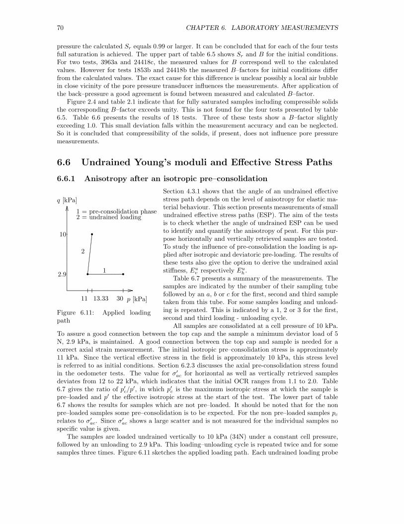
70 CHAPTER 6. LABORATORY MEASUREMENTS
pressure the calculated Sr equals 0.99 or larger. It can be concluded that for each of the four testsfull saturation is achieved. The upper part of table 6.5 shows Sr and B for the initial conditions.For two tests, 3963a and 24418c, the measured values for B correspond well to the calculatedvalues. However for tests 1853b and 24418b the measured B–factors for initial conditions differfrom the calculated values. The exact cause for this difference is unclear possibly a local air bubblein close vicinity of the pore pressure transducer influences the measurements. After application ofthe back–pressure a good agreement is found between measured and calculated B–factor.
Figure 2.4 and table 2.1 indicate that for fully saturated samples including compressible solidsthe corresponding B–factor exceeds unity. This is not found for the four tests presented by table6.5. Table 6.6 presents the results of 18 tests. Three of these tests show a B–factor slightlyexceeding 1.0. This small deviation falls within the measurement accuracy and can be neglected.So it is concluded that compressibility of the solids, if present, does not influence pore pressuremeasurements.
6.6 Undrained Young’s moduli and Effective Stress Paths
6.6.1 Anisotropy after an isotropic pre–consolidation
............................................................................................................................................................................................................................................................................ ...................
.....
.....
.....
.....
.....
.....
.....
.....
.....
.....
.....
.....
.....
.....
.....
.....
.....
.....
.....
.....
.....
.....
.....
.....
.....
.....
.....
.....
.....
.....
.....
.....
.....
.....
.....
.....
.....
.....
.....
.....
.....
.....
.....
.....
.....
.....
.....
.....
.....
.....
.....
.....
.....
.....
.....
.....
.....
.....
.....
.....
.....
.....
.....
.....
....................
...................
.....
.....
.....
.....
.....
.....
.....
.....
.....
.....
.....
.....
.....
.....
.....
.....
.....
.....
.....
.....
.....
.....
.....
.....
.....
.....
.....
.....
.....
.....
...
........................................................................................................................................•
•
•2.9
10
q [kPa]
p [kPa]11 13.33 30
.............
.............
.............
...
1
2
1 = pre-consolidation phase2 = undrained loading
Figure 6.11: Applied loadingpath
Section 4.3.1 shows that the angle of an undrained effectivestress path depends on the level of anisotropy for elastic ma-terial behaviour. This section presents measurements of smallundrained effective stress paths (ESP). The aim of the testsis to check whether the angle of undrained ESP can be usedto identify and quantify the anisotropy of peat. For this pur-pose horizontally and vertically retrieved samples are tested.To study the influence of pre-consolidation the loading is ap-plied after isotropic and deviatoric pre-loading. The results ofthese tests also give the option to derive the undrained axialstiffness, Euv respectively Euh .
Table 6.7 presents a summary of the measurements. Thesamples are indicated by the number of their sampling tubefollowed by an a, b or c for the first, second and third sampletaken from this tube. For some samples loading and unload-ing is repeated. This is indicated by a 1, 2 or 3 for the first,second and third loading - unloading cycle.
All samples are consolidated at a cell pressure of 10 kPa.To assure a good connection between the top cap and the sample a minimum deviator load of 5N, 2.9 kPa, is maintained. A good connection between the top cap and sample is needed for acorrect axial strain measurement. The initial isotropic pre–consolidation stress is approximately11 kPa. Since the vertical effective stress in the field is approximately 10 kPa, this stress levelis referred to as initial conditions. Section 6.2.3 discusses the axial pre-consolidation stress foundin the oedometer tests. The value for σ′
ac for horizontal as well as vertically retrieved samplesdeviates from 12 to 22 kPa, which indicates that the initial OCR ranges from 1.1 to 2.0. Table6.7 gives the ratio of p′c/p
′, in which p′c is the maximum isotropic stress at which the sample ispre–loaded and p′ the effective isotropic stress at the start of the test. The lower part of table6.7 shows the results for samples which are not pre–loaded. It should be noted that for the nonpre–loaded samples some pre–consolidation is to be expected. For the non pre–loaded samples pcrelates to σ′
ac. Since σ′ac shows a large scatter and is not measured for the individual samples no
specific value is given.The samples are loaded undrained vertically to 10 kPa (34N) under a constant cell pressure,
followed by an unloading to 2.9 kPa. This loading–unloading cycle is repeated twice and for somesamples three times. Figure 6.11 sketches the applied loading path. Each undrained loading probe

6.6
.U
ND
RA
INE
DY
OU
NG
’SM
OD
ULI
AN
DE
FFE
CT
IVE
ST
RE
SS
PAT
HS
71
Table 6.6: Descriptive parameters for the conducted triaxial testsparameter unity test number
1853a 1136c 4588a 24076 24482a 24482b 24439bver hor ver hor hor hor hor
W ai [ - ] 4.34 ± 0.008 6.25 ± 0.013 5.53 ± 0.006 5.54 ± 0.013 5.48 ± 0.013 6.23 ± 0.02 5.61 ± 0.012
ρi [t/m3] 1.06 ± 0.02 1.02 ± 0.02 1.03 ± 0.02 1.04 ± 0.02 1.02 ± 0.02 0.99 ± 0.02 1.02 ± 0.008ρbs [t/m3] 1.74 ± 0.009 1.66 ± 0.005 1.65 ± 0.003 1.64 ± 0.004 1.61 ± 0.005 1.61 ± 0.0015 1.60 ± 0.0008eci [ - ] 7.7 ± 0.04 10.9 ± 0.04 9.4 ± 0.04 9.3 ± 0.04 9.3 ± 0.04 10.7 ± 0.04 9.4 ± 0.02nci [ - ] 0.89 ± 0.003 0.92 ± 0.002 0.90 ± 0.002 0.90 ± 0.003 0.90 ± 0.003 0.91 ± 0.002 0.90 ± 0.001Scri [ - ] 0.97 ± 0.01 0.96 ± 0.008 0.97 ± 0.007 0.97 ± 0.009 0.95 ± 0.009 0.93 ± 0.007 0.96 ± 0.004Bi [ - ] 0.89 0.93 0.88 0.96 0.91 0.62 0.07Bfinal [ - ] 0.99 1.03 1.00 1.00 1.01 0.79
4590a 1853b 3963a 24418b 24418c 3963b 24482cver ver ver hor hor ver hor
W ai [ - ] 5.27 ± 0.005 5.56 ± 0.006 5.05 ± 0.015 4.9 ± 0.2 5.35 ± 0.02 5.6 ± 0.3 6.06 ± 0.007
ρi [t/m3] 1.01 ± 0.02 0.99 ± 0.02 1.04 ± 0.02 1.01 ± 0.002 1.03 ± 0.002 1.03 ± 0.002 1.06 ± 0.001ρbs [t/m3] 1.67 ± 0.004 1.67 ± 0.001 1.81 ± 0.005 1.70 ± 0.0004 1.64 ± 0.0009 1.69 ± 0.004 1.69 ± 0.004eci [ - ] 9.3 ± 0.04 10.1 ± 0.3 9.6 ± 0.012 9.0 ± 0.03 9.0 ± 0.007 9.2 ± 0.01 10.28 ± 0.006nci [ - ] 0.90 ± 0.002 0.91 ± 0.002 0.906 ± 0.0008 0.906 ± 0.0004 0.900 ± 0.0005 0.902 ± 0.0009 0.911 ± 0.0004Scri [ - ] 0.94 ± 0.007 0.92 ± 0.03 0.96 ± 0.007 0.94 ± 0.003 0.97 ± 0.005 0.96 ± 0.009 1.00 ± 0.004Bi [ - ] 0.74 0.72 0.92 0.62 0.90 0.63 0.79Bfinal [ - ] 0.99 0.99 0.99 0.95 0.99 0.98 0.97
1316a 2590a 2590b 22726aver ver ver hor
W ai [ - ] 5.37 ± 0.007 4.06 ± 0.01 4.60 ± 0.002 4.56 ±0.008
ρi [t/m3] 1.06 ± 0.001 1.09 ± 0.001 1.08 ± 0.001 1.05 ± 0.001ρbs [t/m3] 1.64 ± 0.005 1.76 ± 0.004 1.61 ± 0.004 1.66 ± 0.003eci [ - ] 8.90 ± 0.007 7.19 ± 0.008 8.31 ± 0.01 7.81 ± 0.007nci [ - ] 0.899 ± 0.0005 0.878 ± 0.0006 0.893 ± 0.0009 0.886 ± 0.0006Scri [ - ] 0.99 ± 0.005 0.99 ± 0.006 1.0 ± 0.01 0.97 ± 0.004Bi [ - ] 0.87 0.90 0.95 0.63Bfinal [ - ] 0.98 0.98 1.04 0.98
a = derived from remaining partsb = measured after finalising the testc = calculated by equation (6.6) under the assumption of incompressible solidsver = vertically retrieved samplehor = horizontally retrieved sample
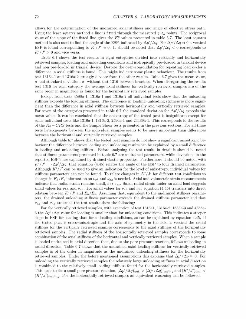
72 CHAPTER 6. LABORATORY MEASUREMENTS
allows for the determination of the undrained axial stiffness and angle of effective stress path.Using the least squares method a line is fitted through the measured q–εa points. The reciprocalvalue of the slope of the fitted line gives the Eua values presented in table 6.7. The least squaresmethod is also used to find the angle of the ESP, indicated by ∆p′/∆q. For ∆p′/∆q ≈ 0 a verticalESP is found corresponding to K ′/J ′ ≈ 0. It should be noted that ∆p′/∆q < 0 corresponds toK ′/J ′ > 0 and vice versa.
Table 6.7 shows the test results in eight categories divided into vertically and horizontallyretrieved samples, loading and unloading conditions and isotropically pre–loaded in triaxial deviceand non pre–loaded in triaxial device. Despite the over–consolidation for repeating load cycles adifference in axial stiffness is found. This might indicate some plastic behaviour. The results fromtest 1316a-1 and 1316a-2 strongly deviate from the other results. Table 6.7 gives the mean value,µ and standard deviation, σ, without test 1316 between brackets. When disregarding the resultstest 1316 for each category the average axial stiffness for vertically retrieved samples are of thesame order in magnitude as found for the horizontally retrieved samples.
Except from tests 4588a-1, 1316a-1 and 1316a-2 all individual tests show that the unloadingstiffness exceeds the loading stiffness. The difference in loading–unloading stiffness is more signif-icant than the difference in axial stiffness between horizontally and vertically retrieved samples.For seven of the categories presented in table 6.7 the standard deviation for ∆p′/∆q exceeds themean value. It can be concluded that the anisotropy of the tested peat is insignificant except forsome individual tests like 1316a-1, 1316a-2, 2590a-1 and 24439a-1. This corresponds to the resultsof the K0 −CRS tests and the Simple Shear tests presented in the previous sections. For all thesetests heterogeneity between the individual samples seems to be more important than differencesbetween the horizontal and vertically retrieved samples.
Although table 6.7 shows that the tested peat samples do not show a significant anisotropic be-haviour the difference between loading and unloading results can be explained by a small differencein loading and unloading stiffness. Before analysing the test results in detail it should be notedthat stiffness parameters presented in table 6.7 are undrained parameters, while deviations in thereported ESP’s are explained by drained elastic properties. Furthermore it should be noted, withK ′/J ′ = -∆p′/∆q, that equation (4.45) relates the angle of the ESP to four drained parameters.Although K ′/J ′ can be used to give an indication for the level of anisotropy, individual values forstiffness parameters can not be found. To relate changes in K ′/J ′ for different test conditions tochanges in Eh/Ev information on νvh and νhh is needed. Axial and volumetric strain measurementsindicate that radial strain remains small, e ≈ εzz. Small radial strain under an axial load suggestssmall values for νhh and νvh. For small values for νvh and νhh equation (4.45) transfers into directrelation between K ′/J ′ and Eh/Ev. Assuming that, equivalent to the undrained stiffness parame-ters, the drained unloading stiffness parameter exceeds the drained stiffness parameter and thatνvh and νhh are small the test results show the following:
For the vertically retrieved samples, with exception of test 1316a1, 1316a-2, 1853a-3 and 4588a-3 the ∆p′/∆q–value for loading is smaller than for unloading conditions. This indicates a steeperslope in ESP for loading than for unloading conditions, as can be explained by equation 4.45. Ifthe tested peat is cross–anisotropic and the axis of symmetry in the field is vertical the radialstiffness for the vertically retrieved samples corresponds to the axial stiffness of the horizontallyretrieved samples. The radial stiffness of the horizontally retrieved samples corresponds to somecombination of the axial stiffness of the horizontal and vertically retrieved samples. When a sampleis loaded undrained in axial direction then, due to the pore pressure reaction, follows unloading inradial direction. Table 6.7 shows that the undrained axial loading stiffness for vertically retrievedsamples is of the order in magnitude as the undrained unloading stiffness for the horizontallyretrieved samples. Under the before mentioned assumptions this explains that ∆p′/∆q ≈ 0. Forunloading the vertically retrieved samples the relatively large unloading stiffness in axial directionis combined to the relatively small loading stiffness found for the horizontally retrieved samples.This leads to the a small pore pressure reaction, (∆p′/∆q)unl. > (∆p′/∆q)loading and (K ′/J ′)unl. <(K ′/J ′)loading. For the horizontally retrieved samples an equivalent reasoning can be followed.

6.6
.U
ND
RA
INE
DY
OU
NG
’SM
OD
ULI
AN
DE
FFE
CT
IVE
ST
RE
SS
PAT
HS
73
Table 6.7: Axial stiffness and ∆p′/∆q–values for vertically and horizontally retrieved samples, µ = mean value, σ = standard deviationvertically retrieved samples horizontally retrieved samples
test loading unloading test loading unloadingnr Eua ∆p′/∆q p′c/p
′ Eua ∆p′/∆q p′c/p′ nr Eua ∆p′/∆q p′c/p
′ Eua ∆p′/∆q p′c/p′
[kPa] [ - ] [ - ] [kPa ] [ - ] [ - ] [kPa] [ - ] [ - ] [kPa] [ - ] [ - ]4590-1 1791 -0.013 2.36 2190 0.007 2.32 24076-1 1202 -0.037 2.65 2035 -0.018 2.221316a-1 3419 -0.22 2.88 3612 -0.25 3.13 24076-2 1714 -0.0005 2.75 1798 -0.002 2.281316a-2 3504 -0.26 2.66 3470 -0.26 3.13 24076-3 1607 -0.007 2.92 1875 0.09 2.341853a-1 1722 0.038 2.67 2086 0.057 2.23 24439a-3 1785 -0.037 2.33 2113 -0.041 2.331853a-2 2123 0.040 2.65 2338 0.059 2.201853a-3 1385 0.033 2.73 1691 -0.002 1.914588a-1 1618 -0.065 2.19 1293 -0.014 1.764588a-2 1568 -0.071 2.23 1867 -0.046 1.844588a-3 1799 -0.049 2.22 2136 -0.054 1.85µ 2103 -0.063 2.51 2298 -0.056 2.26 1577 -0.020 2.66 1955 0.0073 2.29
(1715)1 (-0.012)1 (1943)1 (0.001)1
σ 796 0.11 770 0.12 261 0.019 144 0.057(231)1 (0.05)1 (357)1 (0.044)1
4590a-1 1224 0.011 - 1992 0.089 - 24439a-1 1030 0.13 - 1319 0.10 -2590a-1 680 -0.151 - 893 -0.026 - 24482a-1 761 -0.021 - 853 0.053 -2590a-2 792 -0.041 - 832 -0.009 - 24482b-1 743 -0.091 - 1124 0.042 -2590b-1 1084 -0.090 - 1478 -0.010 - 24482c-1 834 -0.080 - 1109 0.041 -2590b-2 1334 -0.016 - 1469 -0.0017 - 22726a-1 991 -0.049 - 1565 0.044 -
22726a-2 1352 0.007 - 1591 0.031 -µ 1023 -0.057 1333 0.0085 952 -0.017 1260 0.052
(1109)2 (-0.034)2
σ 279 0.064 479 0.046 229 0.080 287 0.025(235)2 (0.042)2
1 = without tests 1316a-1 and 1316a-22 without test 2590a-1

74 CHAPTER 6. LABORATORY MEASUREMENTS
Table 6.8: Results on isotropically pre-consolidated samplesloading unloading
axial test Eua ∆p′/∆q p′0/p′ Eua ∆p′/∆q p′0/p
′
direction nr. [kPa] [ - ] [ - ] [kPa] [ - ] [ - ]ver 4590a-1 1224 0.011 - 1992 0.089 -
4590a-2 1983 -0.005 1.74 2809 0.091 1.714590a-3 1791 -0.013 2.36 2190 0.007 2.32
hor 24439a-1 1030 0.13 - 1319 0.10 -24439a-2 1516 -0.032 1.64 1879 -0.031 1.6424439a-3 1785 -0.037 2.32 2113 -0.041 2.5124482b-1 743 -0.09 - 1124 0.04 -24482b-2 2952 -0.011 1.73 2432 0.03 1.73
For a further investigation of the load history on the anisotropy of peat 3 samples are pre–consolidated at different isotropic stress levels. The axial stiffness and ∆p′/∆q value is measuredat p′ = 11 kPa. First without pre–consolidation, next after isotropic pre–consolidation at p = 20kPa and finally after a pre–consolidation at p = 30 kPa. Table 6.8 shows the results.
Table 6.8 shows a small change in ∆p′/∆q for each level of over–consolidation for loading andunloading conditions, with exception of 4590a-1 to 4590a-2 during unloading. This holds for thevertically retrieved samples as well as for the horizontally retrieved samples. The angle of ESPremains small.
6.6.2 Anisotropy after an anisotropic pre–consolidation
To study the influence of load history some samples are consolidated at an anisotropic stresscondition, σhc = 10 kPa and σvc = 65 kPa. After reconsolidation at the same stress conditionsas for the tests presented in table 6.7 the samples are loaded undrained by a small axial load tomeasure the undrained axial stiffness and the undrained effective stress path. Table 6.9 shows theresults.
Table 6.9: Eua and ∆p′/∆q value after pre-loading up to q = 55 kPaloading unloading
axial test Eua ∆p′/∆q σ′vc/σ
′v Eua ∆p′/∆q σ′
vc/σ′v
direction nr [kPa] [ - ] [ - ] [kPa] [ - ] [ - ]ver. 3963b-1 646 -0.46 6.3 1433 -0.29 3.7
3963b-2 1653 -0.34 5.1 1900 -0.26 3.71316a-3 2895 -0.36 4.5 3138 -0.34 3.11316a-4 3255 -0.37 4.2 3081 -0.33 2.9
hor. 24482c-1 1771 -0.19 5.7 - - -22726a-6 1965 -0.25 4.9 2526 -0.35 3.822726a-7 2189 -0.36 4.6 2904 -0.19 3.1
Comparison with table 6.7 shows a remarkable change in ∆p′/∆q value. Due to malfunctioningof the triaxial device an unloading phase could not be conducted for test 24482c-1. Despite the rel-atively large pre-loading the difference between loading and unloading stiffness is still considerable.The ∆p′/∆q value is decreased indicating a clear change in anisotropy. For the vertically retrievedsamples the ∆p′/∆q value for loading is still larger than for unloading which can be explained bya difference in loading and unloading stiffness.
In test 22726a three levels of axial pre-loading are applied to this, horizontally retrieved, sample.Figure 6.12 sketches the loading path. After consolidation at a cell pressure of 11 kPa, the sample

6.6. UNDRAINED YOUNG’S MODULI AND EFFECTIVE STRESS PATHS 75
.................................................................................................................................................................................................................................................................................................................................................................................................................................................................................................................................................................................................................................................................................... ...................
.....
.....
.....
.....
.....
.....
.....
.....
.....
.....
.....
.....
.....
.....
.....
.....
.....
.....
.....
.....
.....
.....
.....
.....
.....
.....
.....
.....
.....
.....
.....
.....
.....
.....
.....
.....
.....
.....
.....
.....
.....
.....
.....
.....
.....
.....
.....
.....
.....
.....
.....
.....
.....
.....
.....
.....
.....
.....
.....
.....
.....
.....
.....
.....
.....
.....
.....
.....
.....
.....
.....
.....
.....
.....
.....
.....
.....
.....
.....
.....
.....
.....
.....
.....
.....
.....
.....
.....
.....
.....
.....
.....
.....
.....
.....
.....
.....
.....
.....
.....
.....
.....
.....
.....
.....
.....
.......................
...................
........................................................................................................................................................................................................................................................................................................................
.............................................................................................................................................................................................................................................................................................................
..............................................................................................................................................................................................................................................................................................................................................................................................................................................................................................................................................................................................
•
•
•
•
a, e, i
b, d
c
f, h
g
2.9
10
29.3
53.5
q [kPa]
p [kPa]11 13.33 19.77 27.4...........
......................
...........
.........
.........
.........
Figure 6.12: Loading path applied in test 22726a, horizontally retrieved sample
is tested at initial conditions, indicated by a in figure 6.12. After consolidation at anisotropicstress conditions indicated by b, c and d small load cycles are applied in phase e. Finally a largeanisotropic pre–consolidation is applied, indicated by f , g and h and small loading cycles areapplied again in phase i. Figure 6.13 gives the stress strain curve and the effective stress pathsfor test phases a, e and i. It should be noted that phase a consists of two undrained loading–unloading cycles without consolidation in between. Phase e consists of three loading–unloadingcycles with a consolidation or swelling in between. The horizontal parts in the ESP and q − εashown in figure 6.13 represent the consolidation / swelling phase. Phase i consists of two undrainedloading-unloading phases. The first without consolidation / swelling phase, the second includes aconsolidation / swelling phase. Table 6.10 gives the results.
Table 6.10: Relation between anisotropy and loading history for test 22726a, horizontally retrievedsample
loading unloadingphase test σ′
ac/σ′a Euh ∆p′/∆q σ′
ac/σ′a Euh ∆p′/∆q
number [ - ] [kPa] [ - ] [ - ] [kPa] [ - ]a 22726a-1 1.6 991 -0.05 1.2 1565 -0.04
22726a-2 1.7 1352 0.007 1.1 1591 0.03122726a-3 3.0 1873 -0.14 2.0 2073 -0.08
e 22726a-4 2.9 2234 -0.12 1.9 2602 -0.0922726a-5 2.8 2864 -0.10 1.9 2929 -0.10
i 22726a-6 4.9 1965 -0.25 3.8 2526 -0.3522726a-7 4.6 2189 -0.36 3.1 2904 -0.19
Table 6.10 clearly shows the decrease in ∆p′/∆q value for increasing σ′ac/σ
′a. The two axial
drained pre–loading cycles give the opportunity to determine the drained axial stiffness. The slopeof the q− εa diagram given in figure 6.13 gives for the unloading part of the first cycle Ea = 1080kPa. The unloading part of the second cycle give Ea = 1000 kPa for the overall slope and Ea =1300 kPa when fitting the middle part. It is remarkable that the axial stiffness shows a negligible

76 CHAPTER 6. LABORATORY MEASUREMENTS
a, e, i = undrained loading phase
b, f = drained loading phase
c, g = creep
d, h = drained unloading phase
0 5 10 15 20 25 30 35
εa [%]
0
5
10
15
20
25
30
35
40
45
50
55
60
q [kPa]
a
b
c
d
e
f
g
h
i
..................
.......
..........
.......................................................................................................................................................................................................................................................................................................................................................................................................................................................................... ...............................................................................................................................................................................................................................................................................................................................................................................................................................
....................................................
.........
..........
.......
..........
.......
..........
.......
..........
.......
..........
.......
......
..............
......
.......
......
.......
.....
.........
......
.......
......
.......
......
......
........
.......
......
........................................................................................................................................................................................................................................................................................................................................................................................................................................................................................................................................................................................................................................................................................................................................................................................................................................................................................................................................................................................................................................................................................................................................................................................................................................................................................................................................................................................................................................................................................................................................................................................................................................................................................................................................................................................................................................................................................................................................................................................................................................................................................................................................................................................................................................................................................................................................................................................................................................................................................................................................................................................................................................................................................................................................................................................................................................................................................................................................................................................................................................................................................................................................................................................................................................................................................................................................................................................................................................................................................................................................................................................................................................................................................................................................................................................
.......
...........
............
.............
................
...........
....................
.............
.............
..............
.........
............
...........................................................................................................................................................................................................................................................................................................................................................................................................................................................................................................................................................................................................................................................................................................................................................................................................................................................................................................................................................................................................................................................................................................................................................................................................................
.............................................................................................................................................................................................................................................................................................................................................................................................................................................................................................................................................................................................................................................................................................................................................................................................................................................................................................................................................................................................................................................................................................................................................................................................................................................................................................................................................................................................................................................................................................................................................................................................................................................................................................................................................................................................................................................................................................................................................................................................................................................................................................................................................................................................................................................................................................................................................................................................................................................................................................................................................................................................................................................................................................................................................................................................................................................................................................................................................................................................................................................................................................................................................................................................................................................................................................................................................................................................................................................................................................................................................................................................................................................................................................................................................................................................................................................................................................................................................................................................................................................................................................................................................................................................................................................................................................................................................
..........
.......
........
.....
........
......
..........
......
..........
......
..................................................................................................................................................................................................................................................................................................................................................................................................................................................................................................................................................................................................................................................................................................................................................................................................................................................................................................................................................................................................................................................................................................................................................................................................................................................................................................................................................................................................................................................................................................................................................................................................................................................................................................................................................................................................................................................................................................
..................
..........
..............
.........
..............
........
...........
............
........
...............
.........
....................................................................................................................................................................................................................................................................................................................................................................................................................................................................................................................................................
9 10 11 12 13 14 15 16
p′ [kPa]
0
1
2
3
4
5
6
7
8
9
10
q [kPa]
⋄ = phase a△ = phase e• = phase i
⋄⋄⋄⋄⋄⋄⋄⋄
⋄⋄⋄⋄⋄⋄⋄⋄⋄⋄⋄
⋄⋄⋄⋄⋄⋄⋄⋄⋄⋄⋄⋄⋄⋄⋄⋄⋄⋄⋄⋄⋄
⋄⋄⋄⋄⋄⋄⋄⋄⋄⋄⋄ ⋄⋄⋄⋄⋄⋄⋄⋄⋄⋄⋄⋄⋄⋄⋄⋄⋄⋄⋄⋄⋄
⋄⋄⋄⋄⋄⋄⋄⋄
⋄⋄⋄⋄
⋄⋄⋄⋄
⋄
⋄
⋄
⋄
⋄⋄⋄⋄⋄
⋄⋄⋄
⋄⋄⋄
⋄⋄⋄⋄
⋄⋄⋄⋄
⋄⋄
⋄⋄⋄⋄
⋄⋄⋄⋄
⋄⋄⋄⋄⋄⋄⋄⋄
⋄⋄
⋄⋄⋄⋄⋄⋄
⋄⋄⋄⋄⋄⋄⋄
⋄⋄⋄⋄
⋄⋄⋄⋄⋄⋄⋄⋄⋄⋄⋄⋄⋄⋄⋄⋄⋄⋄⋄⋄⋄⋄⋄⋄⋄⋄⋄⋄⋄⋄⋄⋄⋄⋄⋄⋄
⋄⋄⋄⋄⋄⋄⋄
⋄⋄⋄⋄⋄⋄⋄
⋄⋄⋄⋄⋄
⋄⋄⋄⋄⋄⋄⋄
⋄⋄⋄
⋄
⋄
⋄⋄⋄⋄⋄⋄⋄
⋄⋄⋄
⋄⋄
⋄⋄
△△△△△△△△△△△△△△
△△△
△△△
△△
△△
△△△△
△△
△△△△
△△△△
△△△△△△△△△△△△
△△△△△△△△△
△△△△△△
△△△
△△△△△
△△△△
△△
△△△△△
△△△△△△
△△△
△△△△△△△△△
△△
△△△△△△
△△△△△△
△△△△△
△△
△△△
△△△
△△△△△△△△△△△
△△△△ △△△
△△
△△△△
△
△△
△△
△△
△ △
△△△△
△△△
△△
△△△△
△△△
△△△
△△
△△
△△△
△△
△△△△
△△△△△△△
△△△△
△△△△△
△△
△△△
△△△△△△△
△△△△△
△△△△
△△△△△△△
△△
△△•
•••••••
••
•••••••
•••••••
•••••••••
••
•••••••••••••••••••••
••••••••••••••••••
••••••••
••••
••••
••••
•••••••
•••••••••••••••
••••••
••
•••••••
••
•••••
•
••••••••
•
••
•••••
•
••
••
••
•••
••••
•••••••••••••
•••••••••••
••••••••••
••
•••
••
••
• •
• ••••
••••
•••••••••
loading unloading
..................................................................................................................................................................................................
.....
.....
.....
.....
.....
.....
.....
.
.....
.....
.....
.....
.....
.....
.....
.
consolidation /swell
Figure 6.13: Stress–strain curve for test 22726a
increase despite considerable axial strain.
6.6.3 Conclusions
Table 6.7 shows that the tested peat initially does not behave anisotropically. This is shown bythe small difference in axial undrained stiffness for horizontally and vertically retrieved samplesand in the low value for ∆p′/∆q. The results correspond to the results for the K0 − CRS testsand the Simple Shear tests. These tests show only minor differences between the horizontally andvertically retrieved samples.
Axial pre–loading causes tilting of the undrained ESP for loading and unloading in the elasticregion; ∆p′/∆q decreases as shown by table 6.9 and 6.10. This indicates an increase in level ofanisotropy. Assuming small values for νhh and νvh it can be concluded that the ratio Er/Eaincreases. This is remarkable since for a large axial pre–loading an increase in Ea and therefore areduction in Er/Ea is to be expected.
Axial pre–loading causes an equivalent increase in level of anisotropy for the vertically as wellas for the horizontally retrieved samples. If there is initially a dominant fibre direction its influenceseems small.
The test results can be explained by a pre–stressing effect of the fibres. The samples areretrieved at shallow depth underneath a horizontal surface. Initially the fibres are not pre–stressed.The samples show only a mild anisotropy. The mild anisotropy can be explained by a smalldifference for loading and unloading stiffness. Due to the axial pre–consolidation fibres are stretchedand entangle into each other. After unloading the fibres remain entangled. When the sample isloaded undrained in axial direction due to pore pressure generation the sample is unloaded in radialdirection. The entangled, pre–stressed, fibres will hardly show radial deformation leading to anincrease in radial stiffness.
Concerning the pre–stressing of the fibres anisotropy (measurements on ∆p′/∆q) is stronglyinfluenced by the load history. It is therefore concluded that the presence of fibres in itself is notenough to explain the anisotropy of peat. Only when the fibres are pre–stressed the sample showsanisotropic behaviour. Therefore, it is to be expected that anisotropy of peat samples strongly

6.7. THE MANDEL–CRYER EFFECT 77
depends on the location at which they are retrieved. It might differ at short distances. For example,samples from underneath an embankment will show a larger degree of anisotropy than the samplesretrieved from the toe of the embankment.
Since the load history plays an important role in the actual anisotropy of the tested peatsamples sample disturbance becomes an important item. When during sample retrieval an axialforce is applied to the samples, e.g. due to friction along the tube and the sample consolidatesunder this axial force the sample might show an increase in anisotropy.
The test results presented in this section show a large scatter, even for samples that come fromthe same sampling tube. It can be concluded that heterogeneity is an important aspect of peatbehaviour.
6.7 The Mandel–Cryer effect
6.7.1 Measurements and analysis
Section 6.6 discusses the results of undrained loading and unloading tests. After some of theundrained loading or unloading phases a consolidation respectively swelling phase is included.Figure 6.14 depicts the pore pressure development during a consolidation and a swelling phase fortest 1853a. The pore pressure developments shown by figure 6.14 are typical for the consolidationand swelling phases applied after undrained loading or unloading phases presented in table 6.7.The pore pressure development measured at the middle of the sample by the needle correspondswell to the pore pressure development found by the external transducer. The first measurement foreach of the pore pressure developments shown by figure 6.14 corresponds to the condition beforeopening the drainage valve. Since t = 0 is not shown on a logarithmic scale the initial value,measured at t = 0− is shown at t = 0.1 s.
0.1 1 10 102 103 104 105
t [s]
0.0
0.1
0.2
0.3
0.4
0.5
σw/σb
◦
∗
consolidation
swelling
◦
◦◦ ◦
◦◦◦◦◦◦◦◦◦◦
◦◦◦◦◦◦◦
◦
◦ ◦◦◦◦◦◦◦◦◦◦◦◦
◦◦◦◦◦◦◦◦◦◦◦◦◦◦◦◦◦◦◦◦◦◦◦◦◦◦◦◦◦◦◦◦◦◦◦◦◦◦◦◦◦◦◦◦◦◦◦◦◦◦◦◦◦◦◦◦◦◦◦◦◦◦◦◦◦◦◦◦◦◦◦◦◦◦◦◦◦◦◦◦◦◦◦◦◦
◦◦◦◦◦◦◦◦◦◦◦◦◦◦◦◦◦◦◦◦◦◦◦◦◦◦◦◦◦◦◦◦◦◦◦◦◦◦◦◦◦◦◦◦◦◦◦◦◦◦◦◦◦◦◦◦◦◦
◦◦◦◦◦◦◦◦◦
◦
◦◦◦◦◦◦◦◦◦◦◦
◦
◦◦◦◦◦
∗
∗ ∗∗∗∗∗∗∗∗∗∗∗∗∗∗∗∗∗∗∗∗∗∗∗∗∗∗∗∗∗∗∗∗∗∗∗∗∗∗∗∗∗∗∗∗∗∗∗∗∗∗∗∗∗∗∗∗∗∗∗∗∗∗∗∗∗∗∗∗∗∗∗∗∗∗∗∗∗
∗∗∗∗∗∗∗∗∗∗∗∗∗∗∗∗∗∗∗∗∗∗∗∗∗∗∗∗∗∗∗∗∗∗∗∗∗∗∗∗∗∗∗∗∗∗∗∗∗∗∗∗∗∗∗∗∗∗∗∗∗∗∗∗∗∗∗∗∗∗∗∗∗∗∗∗∗∗∗∗∗∗∗∗∗∗∗∗∗∗∗∗∗∗∗∗∗∗∗∗∗∗∗∗∗∗∗∗∗∗∗∗∗∗∗∗∗∗∗∗∗∗∗∗∗∗∗∗∗∗∗∗∗∗∗∗∗∗∗∗∗∗∗∗∗∗∗∗∗∗∗∗∗∗∗∗∗∗∗∗∗∗∗∗∗∗∗∗∗∗∗∗∗∗∗∗∗∗∗∗∗∗∗∗∗∗∗∗∗∗∗∗∗∗∗∗∗∗∗∗∗∗∗∗∗∗∗∗∗∗∗∗∗∗∗∗∗∗∗∗∗∗∗∗∗∗∗∗∗∗∗∗∗∗∗∗∗∗∗∗∗∗∗∗∗∗∗∗∗∗∗∗∗∗∗∗∗∗∗∗∗∗∗∗∗∗∗∗∗∗∗∗∗∗∗∗∗∗∗∗∗∗∗∗∗∗∗∗∗∗∗∗∗∗∗∗∗∗∗∗∗∗∗∗∗∗∗∗∗∗∗∗∗∗∗∗∗∗∗∗∗∗∗∗∗∗∗∗∗∗∗∗∗∗∗∗∗∗∗∗∗∗∗∗∗∗∗∗∗∗∗∗∗∗∗∗∗∗∗∗∗∗∗∗∗∗∗∗∗∗∗∗∗∗∗∗∗∗∗∗∗∗∗∗∗∗∗∗∗∗∗∗∗∗∗∗∗∗∗∗∗∗∗∗∗∗∗∗∗∗∗∗∗∗∗∗∗∗∗∗∗∗∗∗∗∗∗∗∗∗∗∗∗∗∗∗∗∗∗∗∗∗∗∗∗∗∗∗∗∗∗∗∗∗∗∗∗∗∗∗∗∗∗∗∗∗∗∗∗∗∗∗∗∗∗∗∗∗∗∗∗∗∗∗∗∗∗∗∗∗∗∗∗∗∗∗∗∗∗∗∗∗∗∗∗∗∗∗∗∗∗∗∗∗∗∗∗∗∗∗∗∗∗∗∗∗∗
Figure 6.14: Typical pore pressure development at the middle of the sample
Figure 6.14 shows an initial σw/σb = 0.3 to 0.33. This corresponds to equation (4.41) forisotropic conditions, K ′/J ′ = 0. Note that sign convention according to section 2.1 is used. Themeasurement of initial pore pressure also corresponds to results presented in table 6.7. Since forthis test is found ∆p′/∆q ≈ 0. After opening the valves the pore pressure drops to σw/σb ≈ 0.25to 0.3. This drop in pore pressure is followed by a small pore pressure peak. The pore pressuredevelopment presented by figure 6.14 is typical for most measurements. A clear Mandel–Cryereffect as predicted by the analytical formulae is not found.

78 CHAPTER 6. LABORATORY MEASUREMENTS
Section 6.6 shows that axial pre–loading causes tilting of the undrained ESP, which can beexplained by an increase in K ′/J ′. Chapter 5 shows that for an increase in K ′/J ′ a larger Mandel–Cyer effect is to be expected. The consolidation or swelling phases for axially pre–consolidatedsamples do not show a clear Mandel–Cryer effect. An exception is found for test 24482c.
Sample 24482c is one of the samples that are axially pre–consolidated. With ∆q = 55 kPathe applied unloading is considerably larger than for the small regular loading phases discussedin section 6.6. Figure 6.15 presents the pore pressure development during this swelling phase. Asmall initial peak can be distinguished from the measurements using the needle. The externaltransducer indicates a monotonic pore pressure decay.
One of the reasons that might explain the absence of a clear Mandel–Cryer effect is found in theequipment used for the tests. Due to large deformations the cell pressure could be not kept constantin some of the tests leading to a reduction in applied loading. The same holds for the level of back–pressure. Due to the large amount of expelled pore water the stress level in the back–pressurepiston rises leading to an initial increase in pore pressure in de drainage system. Although theincrease in drain pressure is temporarily the test conditions no longer correspond to the boundaryconditions for which the analytical solutions are derived. Especially during consolidation or swellingof isotropic loading phases the pore pressure development is influenced by the testing equipment.These phenomena were not found in each test. The measurements shown by figure 6.14 and 6.15are found for a constant cell pressure and back–pressure.
0.1 1 10 102 103 104 105 106
t [s]
0.0
0.2
0.4
0.6
0.8
σw/σb
◦
∗
internal measurements
external measurements◦
◦ ◦◦◦◦◦◦◦◦◦◦◦◦◦◦◦◦◦◦◦◦◦◦◦◦◦◦◦◦◦◦◦◦◦◦◦◦◦◦◦◦◦◦◦◦◦◦◦◦◦◦◦◦◦◦◦◦◦◦◦◦◦◦◦◦◦◦◦◦◦◦◦◦◦◦◦◦◦◦◦◦◦◦◦◦◦◦◦◦◦◦◦◦◦◦◦◦◦◦◦◦◦◦◦◦◦◦◦◦◦◦◦◦◦◦◦◦◦◦◦◦◦◦◦◦◦◦◦◦◦◦◦◦◦◦◦◦◦◦◦◦◦◦◦◦◦◦◦◦◦◦◦◦◦◦◦◦◦◦◦◦◦◦◦◦◦◦◦◦◦◦◦◦◦◦◦◦◦◦◦◦◦◦◦◦◦◦◦◦◦◦◦◦◦◦◦◦◦◦◦◦◦◦◦◦◦◦◦◦◦◦◦◦◦◦◦◦◦◦◦◦◦◦◦◦◦◦◦◦◦◦◦◦◦◦◦◦◦◦◦◦◦◦◦◦◦◦◦◦◦◦◦◦◦◦◦◦◦◦◦◦◦◦◦◦◦◦◦◦◦◦◦◦◦◦◦◦◦◦◦◦◦◦◦◦◦◦◦◦◦◦◦◦◦◦◦◦◦◦◦◦◦◦◦◦◦◦◦◦◦◦◦◦◦◦◦◦◦◦◦◦◦◦◦◦◦◦◦◦◦◦◦◦◦◦◦◦◦◦◦◦◦◦◦◦◦◦◦◦◦◦◦◦◦◦◦◦◦◦◦◦◦◦◦◦◦◦◦◦◦◦◦◦◦◦◦◦◦◦◦◦◦◦◦◦◦◦◦◦◦◦◦◦◦◦◦◦◦◦◦◦◦◦◦◦◦◦◦◦◦◦◦◦◦◦◦◦◦◦◦◦◦◦◦◦◦◦◦◦◦◦◦◦◦◦◦◦◦◦◦◦◦◦◦◦◦◦◦◦◦◦◦◦◦◦◦◦◦◦◦◦◦◦◦◦◦◦◦◦◦◦◦◦◦◦◦◦◦◦◦◦◦◦◦◦◦◦◦◦◦◦◦◦◦◦◦◦◦◦◦◦◦◦◦◦◦◦◦◦◦◦◦◦◦◦◦◦◦◦◦◦◦◦◦◦◦◦◦◦◦◦◦◦◦◦◦◦◦◦◦◦◦◦◦◦◦◦◦◦◦◦◦◦◦◦◦◦◦◦◦◦◦◦◦◦◦◦◦◦◦◦◦◦◦◦◦◦◦◦◦◦◦◦◦◦◦◦◦◦◦◦◦◦◦◦◦◦◦◦◦◦◦◦◦◦◦◦◦◦◦◦◦◦◦◦◦◦◦◦◦◦◦◦◦◦◦◦◦◦◦◦◦◦◦◦◦◦◦◦◦◦◦◦◦◦◦◦◦◦◦◦◦◦◦◦◦◦◦◦◦◦◦◦◦◦◦◦◦◦◦◦◦◦◦◦◦◦◦◦◦◦◦◦◦◦◦◦◦◦◦◦
∗
∗∗∗∗∗∗∗∗∗∗∗∗∗∗∗∗∗∗∗∗∗∗∗∗∗∗∗∗∗∗∗∗∗∗∗∗∗∗∗∗∗∗∗∗∗∗∗∗∗∗∗∗∗∗∗∗∗∗∗∗∗∗∗∗∗∗∗∗∗∗∗∗∗∗∗∗∗∗∗∗∗∗∗∗∗∗∗∗∗∗∗∗∗∗∗∗∗∗∗∗∗∗∗∗∗∗∗∗∗∗∗∗∗∗∗∗∗∗∗∗∗∗∗∗∗∗∗∗∗∗∗∗∗∗∗∗∗∗∗∗∗∗∗∗∗∗∗∗∗∗∗∗∗∗∗∗∗∗∗∗∗∗∗∗∗∗∗∗∗∗∗∗∗∗∗∗∗∗∗∗∗∗∗∗∗∗∗∗∗∗∗∗∗∗∗∗∗∗∗∗∗∗∗∗∗∗∗∗∗∗∗∗∗∗∗∗∗∗∗∗∗∗∗∗∗∗∗∗∗∗∗∗∗∗∗∗∗∗∗∗∗∗∗∗∗∗∗∗∗∗∗∗∗∗∗∗∗∗∗∗∗∗∗∗∗∗∗∗∗∗∗∗∗∗∗∗∗∗∗∗∗∗∗∗∗∗∗∗∗∗∗∗∗∗∗∗∗∗∗∗∗∗∗∗∗∗∗∗∗∗∗∗∗∗∗∗∗∗∗∗∗∗∗∗∗∗∗∗∗∗∗∗∗∗∗∗∗∗∗∗∗∗∗∗∗∗∗∗∗∗∗∗∗∗∗∗∗∗∗∗∗∗∗∗∗∗∗∗∗∗∗∗∗∗∗∗∗∗∗∗∗∗∗∗∗∗∗∗∗∗∗∗∗∗∗∗∗∗∗∗∗∗∗∗∗∗∗∗∗∗∗∗∗∗∗∗∗∗∗∗∗∗∗∗∗∗∗∗∗∗∗∗∗∗∗∗∗∗∗∗∗∗∗∗∗∗∗∗∗∗∗∗∗∗∗∗∗∗∗∗∗∗∗∗∗∗∗∗∗∗∗∗∗∗∗∗∗∗∗∗∗∗∗∗∗∗∗∗∗∗∗∗∗∗∗∗∗∗∗∗∗∗∗∗∗∗∗∗∗∗∗∗∗∗∗∗∗∗∗∗∗∗∗∗∗∗∗∗∗∗∗∗∗∗∗∗∗∗∗∗∗∗∗∗∗∗∗∗∗∗∗∗∗∗∗∗∗∗∗∗∗∗∗∗∗∗∗∗∗∗∗∗∗∗∗∗∗∗∗∗∗∗∗∗∗∗∗∗∗∗∗∗∗∗∗∗∗∗∗∗∗∗∗∗∗∗∗∗∗∗∗∗∗∗∗∗∗∗∗∗∗∗∗∗∗∗∗∗∗∗∗∗∗∗∗∗∗∗∗∗∗∗∗∗∗∗∗∗∗∗∗∗∗∗∗∗∗∗∗∗∗∗∗∗∗∗∗∗∗∗∗∗∗∗∗∗∗∗∗∗∗∗∗∗∗∗∗∗∗∗∗
Figure 6.15: Swelling of test 24482c
Section 5.5 shows the pore pressure development for a transient drain pressure. The extent towhich the peak value is still visible depends on the drain pressure decay. Section 5.5 expressesthe drain pressure decay by an exponential function; σw = σw0exp(−κt). Using the measurementspresented in figure 6.14 a value for κ and the permeability k can be fitted.
In section 6.6 it is concluded that the sample 1853a does not behave anisotropic. This corre-sponds to an initial pore pressure approximately σw/σb = 1/3 given in figure 6.14. The measure-ments can be compared to the analytical solution for isotropic conditions. The analytical solutionshows that the Mandel–Cryer effect found for isotropic conditions strongly depends on the value forthe Poisson’s ratio. Equating the volume of expelled pore water to the total volume deformation,the average radial strain can be derived from measurements by εr = 0.5 ×(e − εa). Section 3.1shows ν = - εr/εa. Initially the sample behaves undrained leading to ν = 0.5. When consolidationdevelops the ν value reaches its drained value. For the tests presented in figure 6.14 a value for νvarying from 0.10 to 0.15 is found. Figure 6.16 shows the results of the fit for isotropic materialbehaviour, E = 1000 kPa and ν = 0.15.
The measurements presented by figure 6.15 can not easily be fitted. After opening the drainage
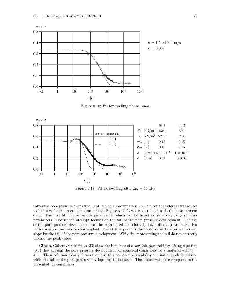
6.7. THE MANDEL–CRYER EFFECT 79
0.1 1 10 102 103 104 105
t [s]
0.0
0.1
0.2
0.3
0.4
0.5
σw/σb
k = 1.5 ×10⁻⁷ m/s
κ = 0.002..............................................................................................................................................................................................................................................................................................................................................................................................................................................................................................................................................................................................................................................................................................................
∗
∗ ∗∗∗∗∗∗∗∗∗∗∗∗∗∗∗∗∗∗∗∗∗∗∗∗∗∗∗∗∗∗∗∗∗∗∗∗∗∗∗∗∗∗∗∗∗∗∗∗∗∗∗∗∗∗∗∗∗∗∗∗∗∗∗∗∗∗∗∗∗∗∗∗
∗∗∗∗∗∗∗∗∗∗
Figure 6.16: Fit for swelling phase 1853a
0.1 1 10 102 103 104 105 106
t [s]
0.0
0.2
0.4
0.6
0.8
σw/σb
◦ measurements
fit 1
fit 2
fit 1 fit 2
Ev [kN/m2] 1300 800
Eh [kN/m2] 2210 1360
νhh [ - ] 0.15 0.15
νvh [ - ] 0.15 0.15
k [m/s] 1.5 × 10⁻⁸ 1 × 10⁻⁷
κ [m/s] 0.01 0.0008
...........................................
....................................................................................................................................................................................................................
..............................
...............................................................................................................................................................................................................................................................................................................................................................................
◦
◦ ◦◦◦◦◦◦◦◦◦◦◦◦◦◦◦◦◦◦◦◦◦◦◦◦◦◦◦◦◦◦◦◦◦◦◦◦◦◦◦◦◦◦◦◦◦◦◦◦◦◦◦◦◦◦◦◦◦◦◦◦◦◦◦◦◦◦◦◦◦◦◦◦◦◦◦◦◦◦◦◦◦◦◦◦◦◦◦◦◦◦◦◦◦◦◦◦◦◦◦◦◦◦◦◦◦◦◦◦◦◦◦◦◦◦◦◦◦◦◦◦◦◦◦◦◦◦◦◦◦◦◦◦◦◦◦◦◦◦◦◦◦◦◦◦◦◦◦◦◦◦◦◦◦◦◦◦◦◦◦◦◦◦◦◦◦◦◦◦◦◦◦◦◦◦◦◦◦◦◦◦◦◦◦◦◦◦◦◦◦◦◦◦◦◦◦◦◦◦◦◦◦◦◦◦◦◦◦◦◦◦◦◦◦◦◦◦◦◦◦◦◦◦◦◦◦◦◦◦◦◦◦◦◦◦◦◦◦◦◦◦◦◦◦◦◦◦◦◦◦◦◦◦◦◦◦◦◦◦◦◦◦◦◦◦◦◦◦◦◦◦◦◦◦◦◦◦◦◦◦◦◦◦◦◦◦◦◦◦◦◦◦◦◦◦◦◦◦◦◦◦◦◦◦◦◦◦◦◦◦◦◦◦◦◦◦◦◦◦◦◦◦◦◦◦◦◦◦◦◦◦◦◦◦◦◦◦◦◦◦◦◦◦◦◦◦◦◦◦◦◦◦◦◦◦◦◦◦◦◦◦◦◦◦◦◦◦◦◦◦◦◦◦◦◦◦◦◦◦◦◦◦◦◦◦◦◦◦◦◦◦◦◦◦◦◦◦◦◦◦◦◦◦◦◦◦◦◦◦◦◦◦◦◦◦◦◦◦◦◦◦◦◦◦◦◦◦◦◦◦◦◦◦◦◦◦◦◦◦◦◦◦◦◦◦◦◦◦◦◦◦◦◦◦◦◦◦◦◦◦◦◦◦◦◦◦◦◦◦◦◦◦◦◦◦◦◦◦◦◦◦◦◦◦◦◦◦◦◦◦◦◦◦◦◦◦◦◦◦◦◦◦◦◦◦◦◦◦◦◦◦◦◦◦◦◦◦◦◦◦◦◦◦◦◦◦◦◦◦◦◦◦◦◦◦◦◦◦◦◦◦◦◦◦◦◦◦◦◦◦◦◦◦◦◦◦◦◦◦◦◦◦◦◦◦◦◦◦◦◦◦◦◦◦◦◦◦◦◦◦◦◦◦◦◦◦◦◦◦◦◦◦◦◦◦◦◦◦◦◦◦◦◦◦◦◦◦◦◦◦◦◦◦◦◦◦◦◦◦◦◦◦◦◦◦◦◦◦◦◦◦◦◦◦◦◦◦◦◦◦◦◦◦◦◦◦◦◦◦◦◦◦◦◦◦◦◦◦◦◦◦◦◦◦◦◦◦◦◦◦◦◦◦◦◦◦◦◦◦◦◦◦◦◦◦◦◦◦◦◦◦
............. ............. ............. ............. ............. ............. ............. ............. ............. ............. ..........................
..........................
.............
.............
.............
..........................
............. ............. ..........
............. .............
Figure 6.17: Fit for swelling after ∆q = 55 kPa
valves the pore pressure drops from 0.61 ×σb to approximately 0.53 ×σb for the external transducerto 0.49 ×σb for the internal measurements. Figure 6.17 shows two attempts to fit the measurementdata. The first fit focuses on the peak value, which can be fitted for relatively large stiffnessparameters. The second attempt focuses on the tail of the pore pressure development. The tailof the pore pressure development can be reproduced for relatively low stiffness parameters. Forboth cases a drain resistance is applied. The fit that predicts the peak correctly gives a too steepslope for the tail of the pore pressure development. While fits representing the tail do not correctlypredict the peak value.
Gibson, Gobert & Schiffman [33] show the influence of a variable permeability. Using equation(6.7) they present the pore pressure development for spherical conditions for a material with χ =4.11. Their solution clearly shows that due to a variable permeability the initial peak is reducedwhile the tail of the pore pressure development is elongated. These observations correspond to thepresented measurements.
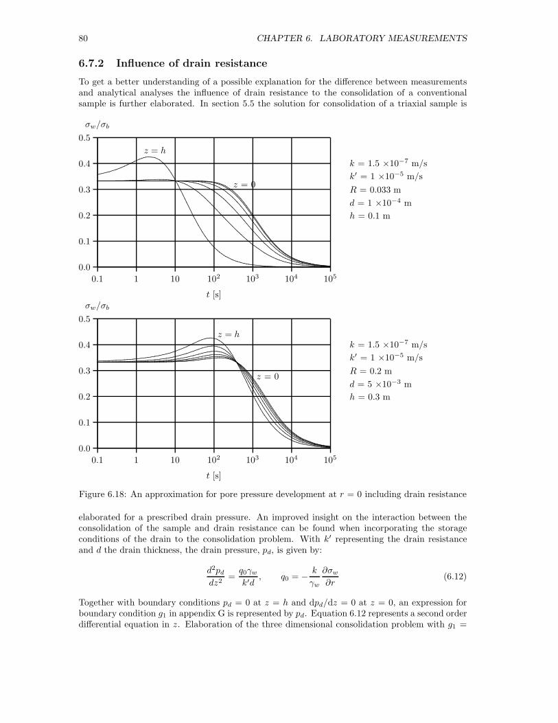
80 CHAPTER 6. LABORATORY MEASUREMENTS
6.7.2 Influence of drain resistance
To get a better understanding of a possible explanation for the difference between measurementsand analytical analyses the influence of drain resistance to the consolidation of a conventionalsample is further elaborated. In section 5.5 the solution for consolidation of a triaxial sample is
0.1 1 10 102 103 104 105
t [s]
0.0
0.1
0.2
0.3
0.4
0.5
σw/σb
k = 1.5 ×10⁻⁷ m/s
k′ = 1 ×10⁻⁵ m/s
R = 0.033 m
d = 1 ×10⁻⁴ m
h = 0.1 m
z = h
z = 0.................................................................................................................................................................................................................................................................................................................................................................................................................................................................................................................................................................................................................................................................................................................................................................................................
.................................................................................................................................................................................................................................................................................................................................................................................................................................................................................................................................................................................................................................................................................................................................................................................................
................................................................................................................................................................................................................................................................................................................................................................................................................................................................................................................................................................................................................................................................................................................................................................................................
.........................................................................................................................................................................................................................................................................................................................................................................................................................................................................................................................................................................................................................................................................................................................................................................................
......................................................................................................................................................................................................................................................................................................................................................................................................................................................................................................................................................................................................................................................................................................................................................................................
.......................................
....................................................................................................
........................................................................................................................................................................................................................................................................................................................................................................................................................................................................................................................................................................................................................................................................................................................
0.1 1 10 102 103 104 105
t [s]
0.0
0.1
0.2
0.3
0.4
0.5
σw/σb
k = 1.5 ×10⁻⁷ m/s
k′ = 1 ×10⁻⁵ m/s
R = 0.2 m
d = 5 ×10⁻³ m
h = 0.3 m
z = h
z = 0
...........................................................................................................................................................................................................................................................................................................................
.....................................................................................................................................................................................................................................................................................................................................................................................................................................................................................
...................................................................................................................................................................................................................................................................................................
...............................................................................................................................................................................................................................................................................................................................................................................................................................................................................................................
..........................................................................................................................................................................................................................................................................
.................................................
...........................................................................................................................................................................................................................................................................................................................................................................................................................................................................................
........................................................................................................................................................................................................................................
..............................................
.....................................
...................................................................................................................................................................................................................................................................................................................................................................................................................................................................................................
..............................................................................................................................................................................................
...............................................
................................
............................
...................................................................................................................................................................................................................................................................................................................................................................................................................................................................................................................................
........................................................................................................................................
........................................................
...................................
................................................................................................................................................................................................................................................................................................................................................................................................................................................................................................................................................................................................................................
Figure 6.18: An approximation for pore pressure development at r = 0 including drain resistance
elaborated for a prescribed drain pressure. An improved insight on the interaction between theconsolidation of the sample and drain resistance can be found when incorporating the storageconditions of the drain to the consolidation problem. With k′ representing the drain resistanceand d the drain thickness, the drain pressure, pd, is given by:
d2pddz2
=q0γwk′d
, q0 = − k
γw
∂σw∂r
(6.12)
Together with boundary conditions pd = 0 at z = h and dpd/dz = 0 at z = 0, an expression forboundary condition g1 in appendix G is represented by pd. Equation 6.12 represents a second orderdifferential equation in z. Elaboration of the three dimensional consolidation problem with g1 =

6.7. THE MANDEL–CRYER EFFECT 81
pd using the Laplace transformation technique leads to an expression in transformed conditions forwhich the inverse transform can not be found.
Figure 6.18 shows the solution found by an approximation technique known as Direct Method.Barends [8] shows that the direct method gives the exact value at about t = 0.5 T , with T thehydrodynamic period. For t < T the direct method underestimates the pore pressure developmentand for t > T the direct method over estimates the pore pressure development. Therefore thisapproximation will not correctly predict the Mandel–Cryer effect and can not be used to reproducemeasurements. However the approximation can be used to visualise the effect of drain resistance.
Figure 6.18 shows pore pressure development for a conventional triaxial sample, R = 0.033 mand h = 0.10 m and for R = 0.2 m and h = 0.3 m. The pore pressure development is given atdifferent levels of z. It should be noted that the pore water dissipates only in radial direction. Sinceat each level a different drain pressure is prescribed at r = R a different pore pressure developmentis found at different levels of z. So the analytical solution predicts a pore pressure gradient invertical direction. At the top of the sample pd = 0 at all stages and therefore at the top of thesample the pore pressure development corresponds to the original solution presented by figure 5.3.At lower levels no Mandel–Cryer peak can be distinguished for a conventional triaxial sample size.The pore pressure development is dominated by the drain resistance. For large sample sizes incombination to a thicker drain with the same drain resistance a clear Mandel–Cryer peak is foundat each level.
Figure 6.18 shows that the influence of drain resistance on the pore pressure developmentreduces for larger sample sizes. So in relation to drain resistance it can be concluded that theMandel–Cryer effect is more easily aroused in large samples than in conventional triaxial tests.The next chapter discusses results of a large scale test.
6.7.3 Conclusions
Only a weak Mandel–Cryer effect is found. This is partly due to mechanical problems of the testequipment. In some tests the pistons were not able to control the cell pressure respectively theback–pressure with required accuracy. For the tests in which the cell pressure and back–pressureis controlled perfectly only a weak Mandel–Cryer effect is found. The pore pressure developmentincluding the weak Mandel–Cryer effect is hard to reproduce by the analytical solutions derived insection 5.
There are two phenomena that might explain the absence of a clear Mandel–Cryer effect in thepore pressure measurements: a variable permeability and a non constant drain pressure. Section6.7.2 shows that size effects play a role regarding the disturbance of drain resistance. For largersamples the influence of drain resistance is small and vice versa.

82 CHAPTER 6. LABORATORY MEASUREMENTS
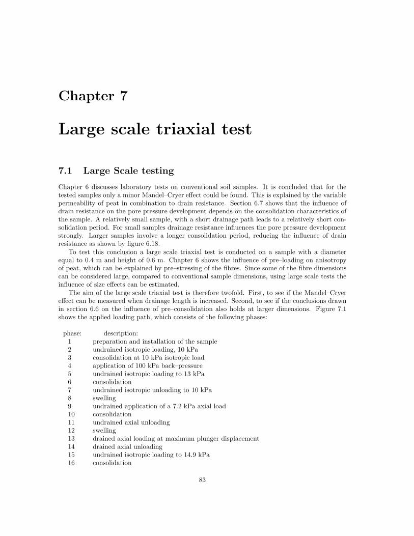
Chapter 7
Large scale triaxial test
7.1 Large Scale testing
Chapter 6 discusses laboratory tests on conventional soil samples. It is concluded that for thetested samples only a minor Mandel–Cryer effect could be found. This is explained by the variablepermeability of peat in combination to drain resistance. Section 6.7 shows that the influence ofdrain resistance on the pore pressure development depends on the consolidation characteristics ofthe sample. A relatively small sample, with a short drainage path leads to a relatively short con-solidation period. For small samples drainage resistance influences the pore pressure developmentstrongly. Larger samples involve a longer consolidation period, reducing the influence of drainresistance as shown by figure 6.18.
To test this conclusion a large scale triaxial test is conducted on a sample with a diameterequal to 0.4 m and height of 0.6 m. Chapter 6 shows the influence of pre–loading on anisotropyof peat, which can be explained by pre–stressing of the fibres. Since some of the fibre dimensionscan be considered large, compared to conventional sample dimensions, using large scale tests theinfluence of size effects can be estimated.
The aim of the large scale triaxial test is therefore twofold. First, to see if the Mandel–Cryereffect can be measured when drainage length is increased. Second, to see if the conclusions drawnin section 6.6 on the influence of pre–consolidation also holds at larger dimensions. Figure 7.1shows the applied loading path, which consists of the following phases:
phase: description:1 preparation and installation of the sample2 undrained isotropic loading, 10 kPa3 consolidation at 10 kPa isotropic load4 application of 100 kPa back–pressure5 undrained isotropic loading to 13 kPa6 consolidation7 undrained isotropic unloading to 10 kPa8 swelling9 undrained application of a 7.2 kPa axial load10 consolidation11 undrained axial unloading12 swelling13 drained axial loading at maximum plunger displacement14 drained axial unloading15 undrained isotropic loading to 14.9 kPa16 consolidation
83
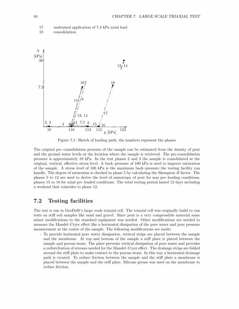
84 CHAPTER 7. LARGE SCALE TRIAXIAL TEST
17 undrained application of 7.4 kPa axial load18 consolidation
......................................................................................... ...................................................................................................................................................................................................................................................................................................................................................... .............................................................................................. ...................
.....
.....
.....
.....
.....
.....
.....
.....
.....
.....
.....
.....
.....
.....
.....
.....
.....
.....
.....
.....
.....
.....
.....
.....
.....
.....
.....
.....
.....
.....
.....
.....
.....
.....
.....
.....
.....
.....
.....
.....
.....
.....
.....
.....
.....
.....
.....
.....
.....
.....
.....
.....
.....
.....
.....
.....
.....
.....
...........
.....
...........
.....
...
........
........
......................
......................
......................
......................
......................
.....
.....
.....
.....
.....
.....
.....
.....
.....
.....
.....
.....
.....
.....
.....
.....
.....
.....
.....
.....
.....
.....
.....
.....
.....
.....
.....
.....
.....
.....
.....
.....
.....
.....
.....
.....
.....
.....
.....
........................
...................
.......................... .................... ...................
.......................... ........ .......................... ........ .......................... ................... ...................
.......................... ........ .......................... ........ ................... ................... .................................................................................................................
.....
...................................................................................................................................................................................
...................
............................................................
..................................
..................................
..................................
...........................
...................
............................................................
..................................
..................................
..................................
.......................................
.....
.....
....
...................
.......................... ........ .......................... ........ .......................... ........ ................................. ................... .....
....................................................................................................................................................................................................
...................
......................................................
...................
• • • •
••
•13, 14
2, 3 4 8 12 67,5
9
10
11
13, 14
15 16
17
18
10 110 113 115 123
7.2
39
p [kPa]
q
[kPa]
Figure 7.1: Sketch of loading path, the numbers represent the phases
The original pre–consolidation pressure of the sample can be estimated from the density of peatand the ground water levels at the location where the sample is retrieved. The pre-consolidationpressure is approximately 10 kPa. In the test phases 2 and 3 the sample is consolidated at theoriginal, vertical, effective stress level. A back–pressure of 100 kPa is used to improve saturationof the sample. A stress level of 100 kPa is the maximum back–pressure the testing facility canhandle. The degree of saturation is checked in phase 5 by calculating the Skempton B factor. Thephases 5 to 12 are used to derive the level of anisotropy of peat for non pre–loading conditions,phases 15 to 18 for axial pre–loaded conditions. The total testing period lasted 12 days includinga weekend that coincides to phase 12.
7.2 Testing facilities
The test is run in GeoDelft’s large–scale triaxial cell. The triaxial cell was originally build to runtests on stiff soil samples like sand and gravel. Since peat is a very compressible material someminor modifications to the standard equipment was needed. Other modifications are needed tomeasure the Mandel–Cryer effect like a horizontal dissipation of the pore water and pore pressuremeasurement at the centre of the sample. The following modifications are made:
- To provide horizontal pore water dissipation, vertical strips are placed between the sampleand the membrane. At top and bottom of the sample a stiff plate is placed between thesample and porous stone. The plate prevents vertical dissipation of pore water and providesa redistribution of stresses needed for the Mandel–Cryer effect. The drainage strips are foldedaround the stiff plate to make contact to the porous stone. In this way a horizontal drainagepath is created. To reduce friction between the sample and the stiff plate a membrane isplaced between the sample and the stiff plate. Silicone grease was used on the membrane toreduce friction.
7.3. THE TESTED PEAT SAMPLE 85
- A transducer is connected at the centre of the top plate and protrudes 3 cm from the plateinto the sample. This transducer is used to register the Mandel–Cryer effect.
- The plunger displacement provides the vertical deformation of the sample. Therefore contactbetween the plunger and the sample needs to be assured at all test phases. A minimumdeviator load is maintained at each phase. Initially a minimum load of 0.07 kN (0.5 kPa)was applied. After solving some technical problems in controlling the plunger the minimumload could be increased to 0.30 kN (2.2 kPa).
- The original equipment is meant for testing stiff material. To cope with the expected rela-tively large deformations, a smaller sample height is chosen and the plunger is elongated by15 cm.
- The expelled pore water is collected in a barrel, the cell water is connected to a burette. Theheight of the burette and barrel can be adjusted by hand. For drained conditions, the waterlevel inside the barrel dictates the pore pressure inside the sample. The water level insidethe burette provides the cell pressure. By adjusting the difference in water level betweenthe barrel and burette an isotropic effective stress is applied on the sample. The volume ofexpelled pore water is measured by measuring the weight of the barrel.
- The back–pressure is applied by increasing the air pressure at the top of barrel and burette.By connecting the barrel and burette at the top deviations in air pressure in barrel andburette are prevented. The level of maximum back–pressure, 100 kPa, is dictated by thestrength of the cell.
- The radial deformations are measured using a hand held laser device. Black spots were placedon the membrane. At regular interval the distance between the black spots and the cell wasmeasured providing an estimate of the radial deformation.
7.3 The tested peat sample
The sample was taken by using a plastic tube with an inner diameter of 0.42 m and a height of1.20 m. The sample was taken from the inner core of a secondary peat dike in Wilnis. The sampleis clearly not homogeneous. The lower part consists of organic clay. The upper part has a darkcolour, indicating a larger degree of humification. The middle section is selected for testing. Theheight of the sample is trimmed using an iron wire to cut the sample from the clayey part and thedark coloured part. The radial dimension of the sample is chosen equal to inner radius of the tube.So no trimming is needed in the radial direction. In the von Post classification [69] the sample canbe described as a von Post type II peat.
Table 7.1 presents the initial and final sample dimensions and weight. The diameter is calcu-lated using the perimeter measurements. The deviation mentioned in table 7.1 follows from themeasurement accuracy.
Table 7.1: Initial and final sample dimensionsparameter unity initial final
value valueperimeter [ m ] 1.31 ± 0.005 1.32 ± 0.005diameter [ m ] 0.42 ± 0.005 0.42 ± 0.005height [ m ] 0.61 ± 0.005 0.50 ± 0.005weight [kg] 77.5 ± 0.05 67.4 ± 0.05volume [m3] 0.082 ± 0.0007 0.070 ± 0.0002density [kg/m3] 940 ± 4 960 ± 6

86 CHAPTER 7. LARGE SCALE TRIAXIAL TEST
Figure 7.2: a) Sample before trimming b) Drainage strips, top plate and porous stone c) Top plateand pore pressure transducer d) Complete set-up
After completion of the test, the sample is cut in vertical direction. Ten small samples arecut from the inner core. From each small sample the water content, W , the loss on ignition, N ,the solid density, ρs, and the CaCO3 content are measured. Table 7.2 presents the results. Thestandard deviation mentioned in table 7.2 follows from statistics.
The samples a1 to a5 and b1 to b5 represent a cross section of the large sample. Samples a1and b1 are collected at the top while a5 and b5 are collected at the bottom. Table 7.2 shows alarger density and a lower loss on ignition for the samples b4 and b5. This corresponds to theobservation that the lower part of the sample contains more clay. The last rows of table 7.2 presentthe average value and the standard deviation. Since the samples b4 and b5 are clearly differentfrom the rest, the average value and standard deviation are given without the samples b4 and b5between brackets.
The properties of table 7.2 and sample dimensions presented by the table 7.1 can be used tofind the parameters like porosity and degree of saturation. By definition:
W =Mw
Ms
, M = Mw +Ms, Ms =W + 1
M, Vs =
(W + 1) /M
ρs
Under the assumption of a constant ρs the initial and final values for porosity n, void ratio eand degree of saturation Sr can be found. It should be noted that the initial stage refers to thesituation before the sample was placed in the cell and final stage refers to the situation in whichthe sample was taken from the cell. In both cases the sample will not be fully saturated.
Table 7.1 shows that the sample mainly deforms vertically and hardly any radial deformationsare present. The small change in perimeter leads to a small change in diameter. For the appliedaccuracy the diameter change is negligible. The volume loss can be estimated from the changein height and equals 0.012 m3. The volume reduction is mainly caused by the expelled pore

7.4. TEST RESULTS 87
Table 7.2: Final water content, density and loss on ignitionsample water density Loss on CaCO3
content ignition[ - ] [t/m3] [%] [%]
a1 5.76 1.46 87.1 13.9a2 5.67 1.46 85.8 17.1a3 5.47 1.46 89.6 9.7a4 5.44 1.45 91.8 4.7a5 5.48 1.44 91.9 3.5b1 6.39 1.42 93.0 2.0b2 6.12 1.41 85.9 18.8b3 5.58 1.50 73.4 16.7b4 4.46 1.66 58.9 13.3b5 4.01 1.84 46.8 9.7
µx 5.44 1.51 80 11(5.73)a (1.45)a (87)a
σx 0.67 0.14 16 6(0.34)a (0.03)a (6)a
a = without tests b4 and b5
Table 7.3: Change in porosity, void ratio and degree of saturationSymbol unity initial finalV [m3] 0.082±0.0003 0.070 ± 0.0002Vs [m3] 0.007±0.001 0.007±0.001n [ - ] 0.9 ± 0.02 0.9 ± 0.02e [ - ] 11 ± 2 9 ± 2Sr [ - ] 0.90 ± 3 0.90 ± 3
water. With the density of water ρw = 1000 kg/m3 follows an estimated weight reduction of 12kg. According to the tables 7.1 the difference in initial and final mass equals 10.1 kg. Table 7.3shows that the degree of saturation equal before and after the test when the sample dimensionsand weight were measured. When the exact non-rounded values are used the degree of saturationafter the test is slightly larger than before the test. This difference counts for 0.5 kg of pore water.Including this difference in degree of saturation the difference sample becomes 10.6 kg (10.1 + 0.5)and is in agreement with the volume change of 0.012 m3.
7.4 Test results
7.4.1 Skempton B–factor
Equivalent to the conventional triaxial tests as described in section 6.5 the Skempton B factor isused to check the saturation of the sample. A back–pressure of 100 kPa is applied to improve thedegree of saturation. The phases 2, 5 and 15 include a cell pressure increase, phase 2 without aback–pressure and the phases 5 and 15 with the back–pressure.
Table 7.4 shows the applied cell pressure increase, ∆σc and the pore pressure reaction. Intable 7.4, ∆σw,in indicates the pore pressure measurements inside the sample. The measurementsindicated by ∆σw,ex refer to the drain pressure. The corresponding B–factor is indicated by Binand Bex respectively.
In phase 2 the isotropic load increase is applied two steps. For each step the pore pressure

88 CHAPTER 7. LARGE SCALE TRIAXIAL TEST
Figure 7.3: a) Sample after testing b) Indication of fibre dimension c) Impression of present fibresd) Cross-section after testing
Table 7.4: Measurement of B–factorsymbol unity Phase2 phase 5 phase 15∆σc [kPa] 4.64 4.27∗ 3.08 4.85∆σw,in [kPa] 3.87 4.17 3.20 4.59Bin [ - ] 0.83 0.98∗ 1.04 0.95∆σw,ex [kPa] 4.73 5.38 3.24 4.80Bex [ - ] 1.02 1.26∗ 1.05 0.99∗ = influenced by equipment modifications
reaction is measured, leading to two B–factors for this phase. The accuracy level of the usedpressure transducers is, according to the manufacturer 0.2 % of maximum measurement range.The maximum measurement range is 300 kPa leading to an approximation of the absolute errorin measured pore pressure of ± 0.6 kPa. Since the exact values for ∆σc, ∆σw,in and ∆σw,exfollow from the subtraction of the readings before and after the justification of the cell pressure theabsolute error in ∆σc, ∆σw,in and ∆σw,ex becomes approximately ± 1.2 kPa. The absolute errorin B follows from the summation of the relative error in ∆σc and ∆σw,in, respectively ∆σw,ex.The absolute error in B becomes ± 0.4 to ± 0.8. The relatively low accuracy in B–factor despitethe use of accurate pressure transducers follows from the relatively small load steps. Keeping theachieved accuracy in B–factor measurement in mind it can be concluded that a reasonable degree

7.4. TEST RESULTS 89
of saturation is achieved.
7.4.2 Volume strain
The total volume change of the sample follows from measurement of expelled pore water weight.The expelled pore water is collected in a barrel. During the test the weight of the barrel and wateris measured continuously, providing the volume of expelled water. Assuming the solid particlesof peat to be incompressible, the volume expelled pore water equals to the volume change of thesample. Figure 7.4 shows the volume expelled pore water during the test. Several loading andunloading phases can be distinguished. The final volume of expelled pore water equals 33 dm3.This volume is not in agreement with the difference the initial and final sample mass (10.6 kg) andsample volume (12 dm3) mentioned in section 7.3.
0 5 10 15 20 25 30 35 40 45 50 55 60 65 70 75 80 85
t× 10 000 [s]
−40
−35
−30
−25
−20
−15
−10
−5
0
Volume [m3].....................................................................
...........
.............................................................................................................................................................................................................................................................................................................................................................................................................................................................................................................................................................................................................................................................................................................................................................................................................................................................................................................................................................................................................................................................................................................................................................................................................................................................................................................................................................................................................................................................................................................................................................................................................................................................................................................................................................................
......
.....
.................
............................................................................................................................................................................................................................................................................................................................................................................................................................................................................................................................................................................................................................................................................................................................................................................................................................................................................................................................................................................................................................................................................................................................................................................................................................................................................................................................................................................................................................................................................................................................................................................
.....
............................................................................................................................................................................................................................................................................................................................................................................................................................................................................................................................................
...............................................................................................
.....................................................................................................................................................................................................................................................................................................................................................................................................................................................................................................................................................................................................................................................................................................................................................................................................................................
Figure 7.4: Total volume of expelled pore water
The difference between the total volume loss found by different measurements is remarkable.Leakage might be a possible explanation for the difference in weight of collected pore water andvolume loss of the sample. If somehow cell water enters the drain more water is collected at theend of the drain than expelled from the sample. If leakage occurs a continuous increase in expelledwater weight should be found. Figure 7.4 shows a continuous increase in expelled pore wateruntil approximately 130 000 s. The testing period from approximately 300 000 s and 500 000 scorresponds to a weekend. During this period the cell pressure, back–pressure and vertical loadwas kept constant. In this period the volume of expelled pore water is constant, as shown in figure7.4. So it seems that initially leakage occurred which was stopped during the test. The curve ingraph 7.4 at 130 000 s during phase 4, the application of the back–pressure, possibly indicatesthe moment the leakage was stopped. The back–pressure was applied almost instantaneouslyfollowed by a resting period of approximately 15 hours. The parameters presented in this reportare derived from the phases 5 to 18. There is no indication that the initial leakage did influencethe measurements in the following phases. The total volume of expelled pore water up to 130 000s is 14.7 dm3, leading to a total volume loss during the test of 18.3 dm3. During the application ofthe back–pressure the volume of expelled pore water reduces by 2.6 dm3. This can be explainedby compression of air bubbles inside the sample and by volume change of the tubes connecting thereservoir to the cell. Correcting the amount of expelled pore water for this phenomenon leads toa total volume of expelled pore water of approximately 15.7 dm3.
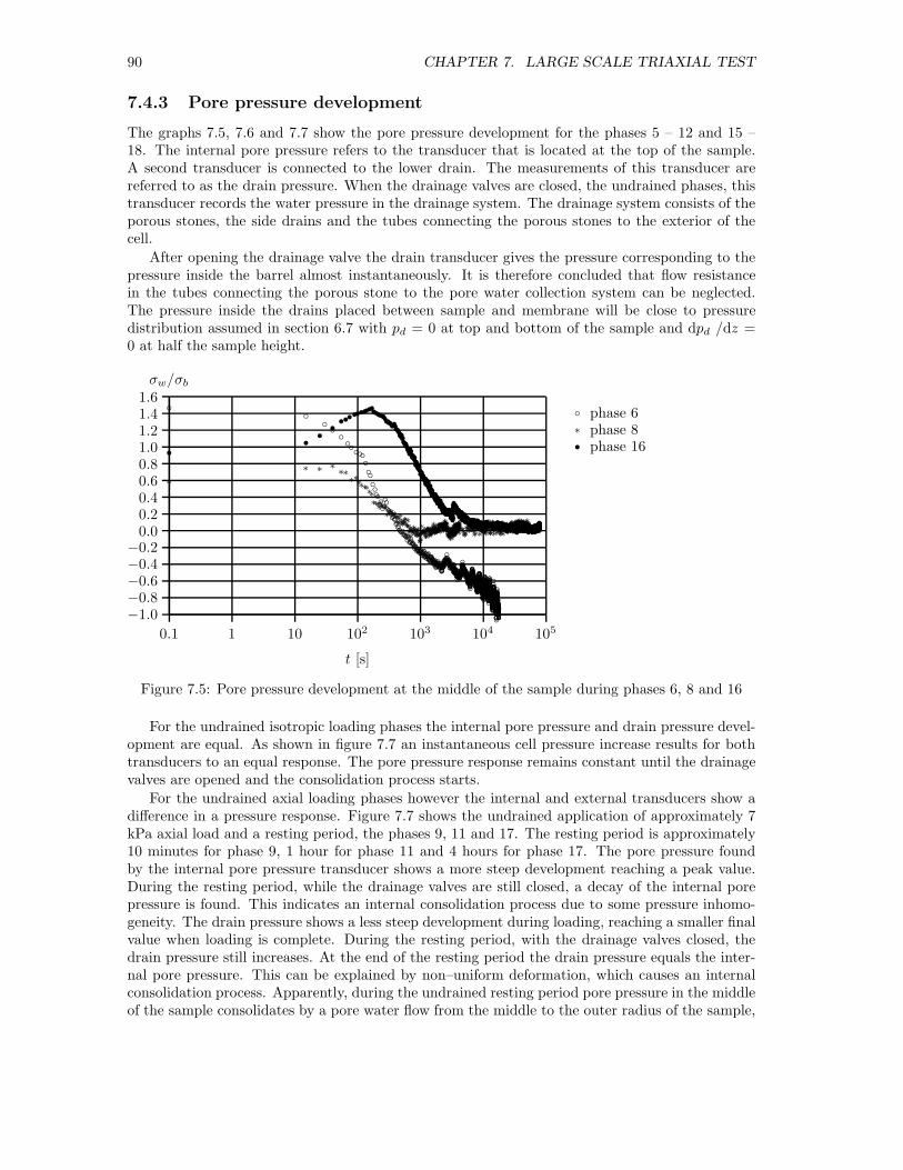
90 CHAPTER 7. LARGE SCALE TRIAXIAL TEST
7.4.3 Pore pressure development
The graphs 7.5, 7.6 and 7.7 show the pore pressure development for the phases 5 – 12 and 15 –18. The internal pore pressure refers to the transducer that is located at the top of the sample.A second transducer is connected to the lower drain. The measurements of this transducer arereferred to as the drain pressure. When the drainage valves are closed, the undrained phases, thistransducer records the water pressure in the drainage system. The drainage system consists of theporous stones, the side drains and the tubes connecting the porous stones to the exterior of thecell.
After opening the drainage valve the drain transducer gives the pressure corresponding to thepressure inside the barrel almost instantaneously. It is therefore concluded that flow resistancein the tubes connecting the porous stone to the pore water collection system can be neglected.The pressure inside the drains placed between sample and membrane will be close to pressuredistribution assumed in section 6.7 with pd = 0 at top and bottom of the sample and dpd /dz =0 at half the sample height.
0.1 1 10 102 103 104 105
t [s]
−1.0−0.8−0.6−0.4−0.2
0.00.20.40.60.81.01.21.41.6σw/σb
•
∗
◦ phase 6phase 8phase 16
•
••
••••••
•••••••••••••••••••••••••••••••••••••••••••••
••••••••••••••••••••••••••••••••••••••••••••••••••••••••••••••••••••••••••••••••••••••••••••••••••••••••••••••••••••••••••••••••••••••••••••••••••••••••••••••••••••••••••••••••••••••••••••••••••••••••••••••••••••••••••••••••••••••••••••••••••••••••••••••••••••••••••••••••••••••••••••••••••••••••••••••••••••••••••••••••••••••••••••••••••••••••••••••••••••••••••••••••••••••••••••••••••••••••••••••••••••••••••••••••••••••••••••••••••••••••••••••••••••••••••••••••••••••••••••••••••••••••••••••••••••••••••••••••••••••••••••••••••••••••••••••••••••••••••••••••••••••••••••••••••••••••••••••••••••••••••••••••••••••••••••••••••••••••••••••••••••••••••••••••••••••••••••••••••••••••••••••••••••••••••••••••••••••••••••••••••••••••••••••••••••••••••••••••••••••••••••••••••••••••••••••••••••••••••••••••••••••••••••••••••••••••••••••••••••••••••••••••••••••••••••••••••••••••••••••••••••••••••••••••••••••••••••••••••••••••••••••••••••••••••••••••••••••••••••••••••••••••••••••••••••••••••••••••••••••••••••••••••••••••••••••••••••••••••••••••••••••••••••••••••••••••••••••••••••••••••••••••••••••••••••••••••••••••••••••••••••••••••••••••••••••••••••••
∗
∗ ∗ ∗∗∗∗∗∗∗∗∗
∗∗∗∗∗∗∗∗∗∗∗∗∗∗∗∗∗∗∗∗∗∗∗∗∗∗∗∗∗∗∗∗∗∗∗∗∗∗∗∗∗∗∗∗∗∗∗∗∗∗∗∗∗∗∗∗∗∗∗∗∗∗∗∗∗∗∗∗∗∗∗∗∗∗∗∗∗∗∗∗∗∗∗∗∗∗∗∗∗∗∗∗∗∗∗∗∗∗∗∗∗∗∗∗∗∗∗∗∗∗∗∗∗∗∗∗∗∗∗∗∗∗∗∗∗∗∗∗∗∗∗∗∗∗∗∗∗∗∗∗∗∗∗∗∗∗∗∗∗∗∗∗∗∗∗∗∗∗∗∗∗∗∗∗∗∗∗∗∗∗∗∗∗∗∗∗∗∗∗∗∗∗∗∗∗∗∗∗∗∗∗∗∗∗∗∗∗∗∗∗∗∗∗∗∗∗∗∗∗∗∗∗∗∗∗∗∗∗∗∗∗∗∗∗∗∗∗∗∗∗∗∗∗∗∗∗∗∗∗
∗∗∗∗∗∗∗∗∗∗∗∗∗∗∗∗∗∗∗∗∗∗∗∗∗∗∗∗∗∗∗∗∗∗∗∗∗∗∗∗∗∗∗∗∗∗∗∗∗∗∗∗∗∗∗∗∗∗∗∗∗∗∗∗∗∗∗∗∗∗∗∗∗∗∗∗∗∗∗∗∗∗∗∗∗∗∗∗∗∗∗∗∗∗∗∗∗∗∗∗∗∗∗∗∗∗∗∗∗∗∗∗∗∗∗∗∗∗∗∗∗∗∗∗∗∗∗∗∗∗∗∗∗∗∗∗∗∗∗∗∗∗∗∗∗∗∗∗∗∗∗∗∗∗∗∗∗∗∗∗∗∗∗∗∗∗∗∗∗∗∗∗∗∗∗∗∗∗∗∗∗∗∗∗∗∗∗∗∗∗∗∗∗∗∗∗∗∗∗∗∗∗∗∗∗∗∗∗∗∗∗∗∗∗∗∗∗∗∗∗∗∗∗∗∗∗∗∗∗∗∗∗∗∗∗∗∗∗∗∗∗∗∗∗∗∗∗∗∗∗∗∗∗∗∗∗∗∗∗∗∗∗∗∗∗∗∗∗∗∗∗∗∗∗∗∗∗∗∗∗∗∗∗∗∗∗∗∗∗∗∗∗∗∗∗∗∗∗∗∗∗∗∗∗∗∗∗∗∗∗∗∗∗∗∗∗∗∗∗∗∗∗∗∗∗∗∗∗∗∗∗∗∗∗∗∗∗∗∗∗∗∗∗∗∗∗∗∗∗∗∗∗∗∗∗∗∗∗∗∗∗∗∗∗∗∗∗∗∗∗∗∗∗∗∗∗∗∗∗∗∗∗∗∗∗∗∗∗∗∗∗∗∗∗∗∗∗∗∗∗∗∗∗∗∗∗∗∗∗∗∗∗∗∗∗∗∗∗∗∗∗∗∗∗∗∗∗∗∗∗∗∗∗∗∗∗∗∗∗∗∗∗∗∗∗∗∗∗∗∗∗∗∗∗∗∗∗∗∗∗∗∗∗∗∗∗∗∗∗∗∗∗∗
◦◦
◦◦◦◦◦◦◦◦◦◦◦◦◦◦◦◦◦◦◦◦◦◦◦◦◦◦◦◦◦◦◦◦◦◦◦◦◦◦◦◦◦◦◦◦◦◦
◦◦◦◦◦◦◦◦◦◦◦◦◦◦◦◦◦◦◦◦◦◦◦◦◦◦◦◦◦◦◦◦◦◦◦◦◦◦◦◦◦◦◦◦◦◦◦◦◦◦◦◦◦◦◦◦◦◦◦◦◦◦◦◦◦◦◦◦◦◦◦◦◦◦◦◦◦◦◦◦◦◦◦◦◦◦◦◦◦◦◦◦◦◦◦◦◦◦◦◦◦◦◦◦◦◦◦◦◦◦◦◦◦◦◦◦◦◦◦◦◦◦◦◦◦◦◦◦◦◦◦◦◦◦◦◦◦◦◦◦◦◦◦◦◦◦◦◦◦◦◦◦◦◦◦◦◦◦◦◦◦◦◦◦◦◦◦◦◦◦◦◦◦◦◦◦◦◦◦◦◦◦◦◦◦◦◦◦◦◦◦◦◦◦◦◦◦◦◦◦◦◦◦◦◦◦◦◦◦◦◦◦◦◦◦◦◦◦◦◦◦◦◦◦◦◦◦◦◦◦◦◦◦◦◦◦◦◦◦◦◦◦◦◦◦◦◦◦◦◦◦◦◦◦◦◦◦◦◦◦◦◦◦◦◦◦◦◦◦◦◦◦◦◦◦◦◦◦◦◦◦◦◦◦◦◦◦◦◦◦◦◦◦◦◦◦◦◦◦◦◦◦◦◦◦◦◦◦◦◦◦◦◦◦◦◦◦◦◦◦◦◦◦◦◦◦◦◦◦◦◦◦◦◦◦◦◦◦◦◦◦◦◦◦◦◦◦◦◦◦◦◦◦◦◦◦◦◦◦◦◦◦◦◦◦◦◦◦◦◦◦◦◦◦◦◦◦◦◦◦◦◦◦◦◦◦◦◦◦◦◦◦◦◦◦◦◦◦◦◦◦◦◦◦◦◦◦◦◦◦◦◦◦◦◦◦◦◦◦◦◦◦◦◦◦◦◦◦◦◦◦◦◦◦◦◦◦◦◦◦◦◦◦◦◦◦◦◦◦◦◦◦◦◦◦◦◦◦◦◦◦◦◦◦◦◦◦◦◦◦◦◦◦◦◦◦◦◦◦◦◦◦◦◦◦◦◦◦◦◦◦◦◦◦◦◦◦◦◦◦◦◦◦◦◦◦◦◦◦◦◦◦◦◦◦◦◦◦◦◦◦◦◦◦◦◦◦◦◦◦◦◦◦◦◦◦◦◦◦◦◦◦◦◦◦◦◦◦◦◦◦◦◦◦◦◦◦◦◦◦◦◦◦◦◦◦◦◦◦◦◦◦◦◦◦◦◦◦◦◦◦◦◦◦◦◦◦◦◦◦◦◦◦◦◦◦◦◦◦◦◦◦◦◦◦◦◦◦◦◦◦◦◦◦◦◦◦◦◦◦◦◦◦◦◦◦◦◦◦◦◦◦◦◦◦◦◦◦◦◦◦◦◦◦◦◦◦◦◦◦◦◦◦◦◦◦◦◦◦◦◦◦◦◦◦◦◦◦◦◦◦◦◦◦◦◦◦◦◦◦◦◦◦◦◦◦◦◦◦◦◦◦◦◦◦◦◦◦◦◦◦◦◦◦◦◦◦◦◦◦◦◦◦◦◦◦◦◦◦◦◦◦◦◦◦◦◦◦◦◦◦◦◦◦◦◦◦◦◦◦◦◦◦◦◦◦◦◦◦◦◦◦◦◦◦◦◦◦◦◦◦◦◦◦◦◦◦◦◦◦◦◦◦◦◦◦◦◦◦◦◦◦◦◦◦◦◦◦◦◦◦◦◦◦◦◦◦◦◦◦◦◦◦◦◦◦◦◦◦◦◦◦◦◦◦◦◦◦◦◦◦◦◦◦◦◦◦◦◦◦◦◦◦◦◦◦◦◦◦◦◦◦◦◦◦◦◦◦◦◦◦◦◦◦◦◦◦◦◦◦◦◦◦◦◦◦◦◦◦◦◦◦◦◦◦◦◦◦◦◦◦◦◦◦◦◦◦◦◦◦◦◦◦◦◦◦◦◦◦◦◦◦◦◦◦◦◦◦◦◦◦◦◦◦◦◦◦◦◦◦◦◦◦◦◦◦◦◦◦◦◦◦◦◦◦◦◦◦◦◦◦◦◦◦◦◦◦◦◦◦◦◦◦◦◦◦◦◦◦◦◦◦◦◦◦◦◦◦◦◦◦◦◦◦◦◦◦◦◦◦◦◦◦◦◦◦◦◦◦◦◦◦◦◦◦◦◦◦◦◦◦◦◦◦◦◦◦◦◦◦◦◦◦◦◦◦◦◦◦◦◦◦◦◦◦◦◦◦◦◦◦◦◦◦◦◦◦◦◦◦◦◦◦◦◦◦◦◦◦◦◦◦◦◦◦◦◦◦◦◦◦◦◦◦◦◦◦◦◦◦◦◦◦◦◦◦◦◦◦◦◦◦◦◦◦◦◦◦◦◦◦◦◦◦◦◦◦◦◦◦◦◦◦◦◦◦◦◦◦◦◦◦◦◦◦◦◦◦◦◦◦◦◦◦◦◦◦◦◦◦◦◦◦◦◦◦◦◦◦◦◦◦◦◦◦◦◦◦◦◦◦◦◦◦◦◦◦◦◦◦◦◦◦◦◦◦◦◦◦◦◦◦◦◦◦◦◦
◦
◦◦◦◦◦◦◦◦◦◦◦
◦◦◦◦◦◦◦◦◦
◦◦◦◦◦◦◦◦◦◦◦◦◦◦◦◦◦◦◦◦◦◦◦◦◦◦◦◦◦◦◦◦◦◦◦◦◦◦◦◦◦◦◦◦◦◦◦◦◦◦◦◦◦◦◦◦◦◦
◦◦◦◦◦◦◦◦◦◦◦◦◦◦◦◦◦◦◦◦◦◦◦◦◦◦◦◦◦◦◦◦◦◦◦◦◦◦◦◦◦◦◦◦◦◦◦◦◦◦◦◦◦◦◦◦◦◦◦
◦
Figure 7.5: Pore pressure development at the middle of the sample during phases 6, 8 and 16
For the undrained isotropic loading phases the internal pore pressure and drain pressure devel-opment are equal. As shown in figure 7.7 an instantaneous cell pressure increase results for bothtransducers to an equal response. The pore pressure response remains constant until the drainagevalves are opened and the consolidation process starts.
For the undrained axial loading phases however the internal and external transducers show adifference in a pressure response. Figure 7.7 shows the undrained application of approximately 7kPa axial load and a resting period, the phases 9, 11 and 17. The resting period is approximately10 minutes for phase 9, 1 hour for phase 11 and 4 hours for phase 17. The pore pressure foundby the internal pore pressure transducer shows a more steep development reaching a peak value.During the resting period, while the drainage valves are still closed, a decay of the internal porepressure is found. This indicates an internal consolidation process due to some pressure inhomo-geneity. The drain pressure shows a less steep development during loading, reaching a smaller finalvalue when loading is complete. During the resting period, with the drainage valves closed, thedrain pressure still increases. At the end of the resting period the drain pressure equals the inter-nal pore pressure. This can be explained by non–uniform deformation, which causes an internalconsolidation process. Apparently, during the undrained resting period pore pressure in the middleof the sample consolidates by a pore water flow from the middle to the outer radius of the sample,

7.4. TEST RESULTS 91
0.1 1 10 102 103 104 105 106
t [s]
−0.2
0.0
0.2
0.4
0.6
0.8
1.0σw/σb
•
∗
◦
phase 10phase 12phase 18• •
• ••••••••••••••••••••••••••••••••••••••••••••••••
••••••••••••••••••••••••••••••••••••••••••••••••••••••••••••••••••••••••••••••••••••••••••••••••••••••••••••••••••••••••••••••••••••••••••••••••••••••••••••••••••
∗∗
∗ ∗ ∗∗∗∗∗∗∗∗∗∗∗∗∗∗∗∗∗∗∗∗∗∗∗∗∗∗∗∗∗
∗∗∗∗∗∗∗∗∗∗∗∗∗∗∗∗∗∗∗∗∗∗∗∗∗∗∗∗∗∗∗∗∗∗∗∗∗∗∗∗∗∗∗∗∗∗∗∗∗∗∗∗∗∗∗∗∗∗∗∗∗∗∗∗∗∗∗∗∗∗∗∗∗∗∗∗∗∗∗∗∗∗∗∗∗∗∗∗∗∗∗∗∗∗∗∗∗∗∗∗∗∗∗∗∗∗∗∗∗∗∗∗∗∗∗∗∗∗∗∗∗∗∗∗∗∗∗∗∗∗∗∗∗∗∗∗∗∗∗∗∗∗∗∗∗∗∗∗∗∗
∗∗∗∗
∗∗∗∗∗∗∗∗∗∗∗∗∗∗∗∗∗∗
∗∗∗∗∗∗∗∗∗∗∗∗∗∗∗∗∗∗∗∗∗∗∗∗∗∗∗∗∗∗∗∗∗∗∗∗∗∗∗∗∗∗∗∗∗∗∗∗∗∗∗∗∗∗∗∗∗∗∗∗∗∗∗∗∗∗∗∗∗∗∗∗∗∗∗∗∗∗∗∗∗∗∗∗∗∗∗∗∗∗∗∗∗∗∗∗∗∗∗∗∗∗∗∗∗∗∗∗∗∗∗∗
∗∗∗∗∗∗∗∗∗∗∗∗∗∗∗∗∗∗∗∗∗∗∗∗∗∗∗∗∗∗∗∗∗∗∗∗∗∗∗∗∗∗∗∗∗∗∗∗∗∗∗∗∗
∗∗∗∗∗∗∗∗∗∗∗∗∗∗∗∗∗∗∗∗∗∗∗∗∗∗∗∗∗∗∗∗∗∗∗∗∗∗∗∗∗∗∗∗∗∗∗∗∗∗∗∗∗∗∗∗∗∗∗∗∗∗∗∗∗∗∗∗∗∗∗∗∗∗∗∗∗∗∗∗∗∗∗∗∗∗∗∗∗∗∗∗∗∗∗∗∗∗∗∗∗∗∗∗∗∗∗∗∗∗∗∗∗∗∗∗∗∗∗∗∗∗∗∗∗∗∗∗∗∗∗∗∗∗∗∗∗∗∗∗∗∗∗∗∗∗∗∗∗∗∗∗∗∗∗∗∗∗∗∗∗∗∗∗∗∗∗∗∗∗∗∗∗∗∗∗∗∗∗∗∗∗∗∗∗∗∗∗∗∗∗∗∗∗∗∗∗∗∗∗∗∗∗∗∗∗∗∗∗∗∗∗∗∗∗∗∗∗∗∗∗∗∗∗∗∗∗∗∗∗∗∗∗∗∗∗∗∗∗∗∗∗∗∗∗∗∗∗∗∗∗∗∗∗∗∗∗∗∗∗∗∗∗∗∗∗∗∗∗∗∗∗∗∗∗∗∗∗∗∗∗∗∗∗∗∗∗∗∗∗∗∗∗∗∗∗∗∗∗∗∗∗∗∗∗∗∗∗∗∗∗∗∗∗∗∗∗∗∗∗∗∗∗∗∗∗∗∗∗∗∗∗∗∗∗∗∗∗∗∗∗∗∗∗∗∗∗∗∗∗∗∗∗∗∗∗∗∗∗∗∗∗∗∗∗∗∗∗∗∗∗∗∗∗∗∗∗∗∗∗∗∗∗∗∗∗∗∗∗∗∗∗∗∗∗∗∗∗∗∗∗∗∗∗∗∗∗∗∗∗∗∗∗∗∗∗∗∗∗∗∗∗∗∗∗∗∗∗∗∗∗∗∗∗∗∗∗∗∗∗∗∗∗∗∗∗∗∗∗∗∗∗∗∗∗∗∗∗∗∗∗∗∗∗∗∗∗∗∗∗∗∗∗∗∗∗∗∗∗∗∗∗∗∗∗∗∗∗∗∗∗∗∗∗∗∗∗∗∗∗∗∗∗∗∗∗∗∗∗∗∗∗∗∗∗∗∗∗∗∗∗∗∗∗∗∗∗∗∗∗∗∗∗∗∗∗∗∗∗∗∗∗∗∗∗∗∗∗∗∗∗∗∗∗∗∗∗∗∗∗∗∗∗∗∗∗∗∗∗∗∗
◦ ◦◦ ◦
◦◦◦◦◦◦◦◦◦◦◦◦◦◦◦◦◦◦◦◦◦◦◦◦◦◦◦◦◦◦◦◦◦◦◦◦◦◦◦◦◦◦◦◦◦◦◦◦◦◦◦◦◦◦◦◦◦◦◦◦◦◦◦◦◦◦◦◦◦◦◦◦◦◦◦◦◦◦◦◦◦◦◦◦◦◦◦◦◦◦◦◦◦◦◦◦◦◦◦◦◦◦◦◦◦◦◦◦◦◦◦◦◦◦◦◦◦◦◦◦◦◦◦◦◦◦◦◦◦◦◦◦◦◦◦◦◦◦◦◦◦◦◦◦◦◦◦◦◦◦◦◦◦◦◦◦◦◦◦◦◦◦◦◦◦◦◦◦◦◦◦◦◦◦◦◦◦◦◦◦◦◦◦◦◦◦◦◦◦◦◦◦◦◦◦◦◦◦◦◦◦◦◦◦◦◦◦◦◦◦◦◦◦
◦◦◦◦◦◦◦◦◦◦◦◦◦◦◦◦◦◦◦◦◦◦◦◦◦◦◦◦◦◦◦◦◦◦◦◦◦◦◦◦◦◦◦◦◦◦◦◦◦◦◦◦◦◦◦◦◦◦◦◦◦◦◦◦◦◦◦◦◦◦◦◦◦◦◦◦◦◦◦◦◦◦◦◦◦◦◦◦◦◦◦◦◦◦◦◦◦◦◦◦◦◦◦◦◦◦◦◦◦◦◦◦◦◦◦◦◦◦◦◦◦◦◦◦◦◦◦◦◦◦◦◦◦◦◦◦◦◦◦◦◦◦◦◦◦◦◦◦◦◦◦◦◦◦◦◦◦◦◦◦◦◦◦◦◦◦◦◦◦◦◦◦◦◦◦◦◦◦◦◦◦◦◦◦◦◦◦◦◦◦◦◦◦◦◦◦◦◦◦◦◦◦◦◦◦◦◦◦◦◦◦◦◦◦◦◦◦◦◦◦◦◦◦◦◦◦◦◦◦◦◦◦◦◦◦◦◦◦◦◦◦◦◦◦◦◦◦◦◦◦◦◦◦◦◦◦◦◦◦◦◦◦◦◦◦◦◦◦◦◦
◦◦◦◦◦◦◦◦◦◦◦◦◦◦◦◦◦◦◦◦◦◦◦◦◦◦◦◦◦◦◦◦◦◦◦◦◦◦◦◦◦◦◦◦◦◦◦◦◦◦◦◦◦◦◦◦◦◦◦◦◦◦◦◦◦◦◦◦◦◦◦◦◦◦◦◦◦◦◦◦◦◦◦◦◦◦◦◦◦◦◦◦◦◦◦◦◦◦◦◦◦◦◦◦◦◦◦◦◦◦◦◦◦◦◦◦◦◦◦◦◦◦◦◦◦◦◦◦◦◦◦◦◦◦◦◦◦◦◦◦◦◦◦◦◦◦◦◦◦◦◦◦◦◦◦◦◦◦◦◦◦◦◦◦◦◦◦◦◦◦◦◦◦◦◦◦◦◦◦◦◦◦◦◦◦◦◦◦◦◦◦◦◦◦◦◦◦◦◦◦◦◦◦◦◦◦◦◦◦◦◦◦◦◦◦◦◦◦◦◦◦◦◦◦◦◦◦◦◦◦◦◦◦◦◦◦◦◦◦◦◦◦◦◦◦◦◦◦◦◦◦◦◦◦◦◦◦◦◦◦◦◦◦◦◦◦◦◦◦◦◦◦◦◦◦◦◦◦◦◦◦◦◦◦◦◦◦◦◦◦◦◦◦◦◦◦◦◦◦◦◦◦◦◦◦◦◦◦◦◦◦◦◦◦◦◦◦◦◦◦◦◦◦◦◦◦◦◦◦◦◦◦◦◦◦◦◦◦◦◦◦◦◦◦◦◦◦◦◦◦◦◦◦◦◦◦◦◦◦◦◦◦◦◦◦◦◦◦◦◦◦◦◦◦◦◦◦◦◦◦◦◦◦◦◦◦◦◦◦◦◦◦◦◦◦◦◦◦◦◦◦◦◦◦◦◦◦◦◦◦◦◦◦◦◦◦◦◦◦◦◦◦◦◦◦◦◦◦◦◦◦◦◦◦◦◦◦◦◦◦◦◦◦◦◦◦◦◦◦◦◦◦◦◦◦◦◦◦◦◦◦◦◦◦◦◦◦◦◦◦◦◦◦◦◦◦◦◦◦◦◦◦◦◦◦◦◦◦◦◦◦◦◦◦◦◦◦◦◦◦◦◦◦◦◦◦◦◦◦◦◦◦◦◦◦◦◦◦◦◦◦◦
Figure 7.6: Pore pressure development at the middle of the sample during phases 10, 12 and 18
0 500 1000 1500 2000 2500 3000 3500 4000
t [s]
0.0
0.2
0.4
0.6
0.8
1.0
1.2
1.4
1.6
σw/σb
•
∗
◦
phase 9
phase 11
phase 17
internal
drain
•
•
•••••••••••••••••••••••••••••••••••••••••••••••••••••••••••••••••••••••••••••••••••••
•
••••••••••••••••••••••••••••••••••••••••••••••••••••••••
••••••••••••••••••••••••••••••
∗
∗
∗∗∗∗∗∗∗∗∗∗∗
∗∗∗∗∗∗∗∗∗∗∗∗∗∗∗∗∗∗∗∗∗∗∗∗∗∗∗∗∗∗∗∗∗∗∗∗∗∗∗∗∗∗∗∗∗∗∗∗∗∗∗∗∗∗∗∗∗∗∗∗∗∗
∗
∗
∗∗∗∗∗∗∗∗∗∗∗∗∗∗∗∗∗∗∗∗∗∗
∗∗∗∗∗∗∗∗∗∗∗∗∗∗∗∗∗∗∗∗∗∗∗∗∗∗∗∗∗∗∗
∗∗∗∗∗∗∗∗∗∗∗∗∗∗∗∗∗∗∗∗
◦◦
◦
◦◦◦◦◦◦◦◦◦◦◦◦◦◦◦◦◦◦◦◦◦◦◦◦◦◦◦◦◦◦◦◦◦◦◦◦◦◦◦◦◦◦◦◦◦◦◦◦◦◦◦◦◦◦◦◦◦◦◦◦◦◦◦◦◦◦◦◦◦◦◦◦◦◦◦◦◦◦◦◦◦◦◦◦◦◦◦◦◦◦◦◦◦◦◦◦◦◦◦◦◦◦◦◦◦◦◦◦◦◦◦◦◦◦◦◦◦◦◦◦◦◦◦◦◦◦◦◦◦◦◦◦◦◦◦◦◦◦◦◦◦◦◦◦◦◦◦◦◦◦◦◦◦◦◦◦◦◦◦◦◦◦◦◦◦◦◦◦◦◦◦◦◦◦◦◦◦◦◦◦◦◦◦◦◦◦◦◦◦◦
◦
◦
◦
◦◦◦◦◦◦◦◦◦◦◦◦◦◦◦◦◦◦◦◦◦◦◦◦◦◦◦◦◦◦◦◦◦◦◦◦◦◦◦◦◦
◦◦◦◦◦◦◦◦◦◦◦◦◦◦◦◦◦◦◦◦◦◦◦◦◦◦◦
◦◦◦◦◦◦◦◦◦◦◦◦◦◦◦◦◦◦◦◦◦◦◦◦◦◦◦◦
◦◦◦◦◦◦◦◦◦◦◦◦◦◦◦◦◦◦◦◦◦◦◦◦◦◦◦◦◦◦◦◦◦
◦◦◦◦◦◦◦◦◦◦◦◦◦◦◦◦◦◦◦◦◦◦◦◦◦◦
◦◦◦◦◦◦◦◦◦◦◦◦◦◦◦◦◦◦◦◦◦◦◦◦◦◦◦◦◦◦◦◦◦◦◦
⋄
△
phase 5
(internal + drain)
phase 15
(internal + drain)
⋄
⋄⋄⋄⋄⋄⋄⋄⋄⋄⋄⋄⋄
⋄
⋄⋄⋄⋄⋄⋄⋄
⋄⋄
⋄⋄⋄⋄
⋄⋄⋄
⋄⋄
⋄⋄⋄⋄⋄⋄⋄⋄
⋄
⋄
⋄⋄
⋄⋄⋄
⋄⋄⋄⋄⋄
⋄⋄
⋄⋄
⋄⋄⋄⋄⋄⋄⋄⋄⋄⋄
⋄⋄
⋄
⋄
⋄
⋄⋄⋄⋄⋄⋄⋄⋄⋄⋄⋄⋄⋄
⋄⋄⋄⋄⋄
⋄⋄⋄⋄⋄⋄⋄
⋄⋄⋄⋄⋄⋄⋄⋄⋄⋄⋄⋄⋄⋄⋄⋄⋄⋄⋄⋄⋄⋄⋄⋄⋄
⋄⋄⋄⋄⋄⋄⋄⋄⋄⋄⋄⋄⋄⋄
⋄
⋄
⋄⋄⋄⋄⋄⋄⋄⋄
⋄⋄⋄
⋄
⋄⋄⋄⋄⋄⋄⋄⋄⋄
⋄⋄⋄⋄⋄⋄⋄⋄⋄⋄⋄⋄⋄⋄⋄⋄⋄⋄⋄
⋄⋄
⋄⋄⋄⋄⋄⋄
⋄⋄
⋄
⋄
⋄
⋄
⋄
⋄⋄⋄⋄
⋄⋄⋄⋄⋄⋄⋄
⋄
⋄⋄⋄⋄⋄⋄⋄⋄⋄⋄⋄⋄
⋄⋄⋄⋄⋄⋄⋄⋄⋄⋄⋄⋄⋄⋄⋄⋄⋄⋄⋄⋄⋄⋄⋄⋄⋄⋄⋄⋄⋄⋄⋄⋄⋄⋄⋄⋄⋄⋄
⋄⋄
⋄⋄⋄⋄
⋄
⋄⋄⋄
⋄⋄⋄⋄⋄
⋄⋄⋄⋄⋄⋄⋄⋄⋄⋄⋄⋄⋄⋄⋄⋄⋄⋄⋄⋄⋄⋄⋄⋄⋄⋄⋄⋄⋄⋄⋄⋄⋄⋄⋄⋄
⋄⋄⋄⋄⋄⋄⋄⋄⋄⋄⋄⋄⋄⋄⋄⋄⋄⋄⋄⋄⋄⋄⋄⋄⋄⋄⋄⋄
⋄⋄⋄⋄⋄⋄⋄⋄⋄⋄⋄⋄⋄⋄⋄⋄⋄⋄⋄⋄⋄⋄⋄⋄⋄⋄⋄⋄⋄⋄⋄
⋄⋄⋄⋄⋄⋄⋄⋄⋄⋄⋄⋄⋄⋄⋄⋄⋄⋄⋄⋄⋄⋄⋄⋄⋄⋄⋄⋄⋄⋄⋄⋄⋄
⋄⋄⋄⋄⋄⋄⋄⋄⋄⋄⋄⋄⋄⋄⋄⋄⋄⋄
⋄⋄⋄⋄⋄⋄⋄⋄⋄
⋄⋄⋄⋄⋄⋄⋄⋄⋄⋄⋄⋄⋄⋄⋄⋄⋄⋄⋄⋄⋄⋄⋄⋄⋄⋄⋄⋄⋄
⋄⋄
⋄
⋄
⋄
⋄
⋄
⋄⋄⋄⋄⋄⋄⋄⋄⋄⋄⋄
⋄
⋄⋄⋄⋄⋄⋄⋄⋄⋄⋄⋄⋄⋄⋄⋄⋄⋄⋄⋄⋄⋄⋄⋄⋄⋄⋄⋄⋄⋄⋄⋄⋄⋄⋄⋄⋄⋄⋄⋄⋄⋄⋄⋄⋄⋄⋄⋄⋄⋄⋄
⋄
⋄
⋄⋄
⋄
⋄
⋄
⋄⋄⋄
△
△
△△△△△△
△△△△△△△△△△△△△△△△△△△△△
△△△△△△△
△△△△△△△△△△△△△△△△△△△
△△△△△△△
△△△△△
△△△△△△△△△△△
△△△△△△△△△△△△△△△△△△△△△△△△△△△△△△△△△△△△△△△△△△△△△△△
△
△△△△△△△△△△△△△△△△△△△△△△△△
△△△△△△△
△△△△△△△△△△△△△△△△△△△△△△△△△△△△△△△△△△△△
△△
△△△△△△△△△△△△
△△
△
△△△△△△△△△△△△△△△△△△△△△
△△△△△△△△△△△△△△△
△△△△△△△△△△△△△△△△
△△△△△△△△△△△△△△△△△△△△△△△△
△△△△△△△△
△△
△△△△△△△△△△△△△△△△△△△△△△△△△△△△△△△△△△△
△△△△△△△△△△△△△△△△△△△△△△△△△△△△△△△△△△△△△△△△△△△△△△△△△△△△△△△△△△△△△△△△△△△△△△△△△△△△△△△△△△△△△△△△△△△△△△△△△△△△△△△△△△△△△△△
△△△△△△△△△△△△△△△△△△△△△△△△△△△△△△△△△△△△△△△△△△△△△△△△△△△△△△△△△△△△△△△△△△△△△△△△△△△△△△△△△△△△△
△△△△△△△△△△△△△△△△△△△△△△△△△△△△△△△△△△△△△△△△△△△△△△△△△△△△△△△△△△△△△△△△△△
Figure 7.7: Pore pressure development during phases 5, 9, 11, 15 and 17
the drains and the porous stone.
Measurements of phase 7 are not presented by figure 7.7 since due to modifications to testequipment no clear pore pressure development is found. Figure 7.6 shows the consolidation of thesample due to an axial pre-load of approximately 7 kPa. Phases 10 and 18 represent a loadingphase, while phase 12 represents an unloading phase. Figure 7.6 clearly shows the Mandel–Cryereffect.
Table 7.5 shows the exact load and pore pressure reaction. The parameters ∆σw,ini and
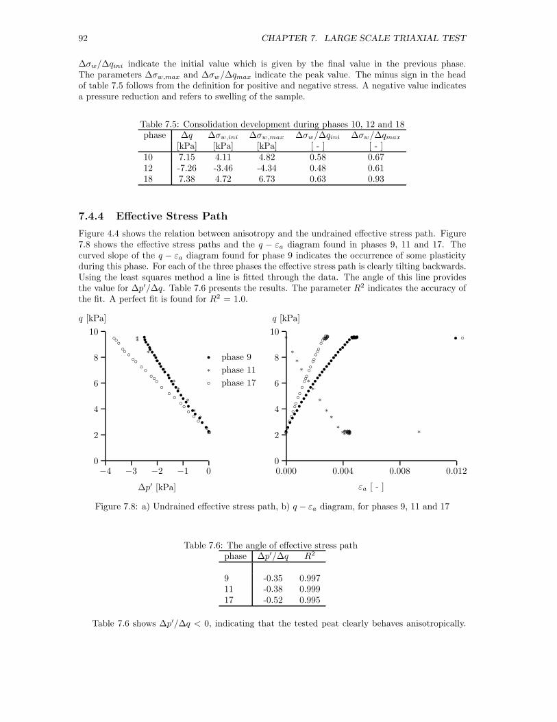
92 CHAPTER 7. LARGE SCALE TRIAXIAL TEST
∆σw/∆qini indicate the initial value which is given by the final value in the previous phase.The parameters ∆σw,max and ∆σw/∆qmax indicate the peak value. The minus sign in the headof table 7.5 follows from the definition for positive and negative stress. A negative value indicatesa pressure reduction and refers to swelling of the sample.
Table 7.5: Consolidation development during phases 10, 12 and 18phase ∆q ∆σw,ini ∆σw,max ∆σw/∆qini ∆σw/∆qmax
[kPa] [kPa] [kPa] [ - ] [ - ]10 7.15 4.11 4.82 0.58 0.6712 -7.26 -3.46 -4.34 0.48 0.6118 7.38 4.72 6.73 0.63 0.93
7.4.4 Effective Stress Path
Figure 4.4 shows the relation between anisotropy and the undrained effective stress path. Figure7.8 shows the effective stress paths and the q − εa diagram found in phases 9, 11 and 17. Thecurved slope of the q − εa diagram found for phase 9 indicates the occurrence of some plasticityduring this phase. For each of the three phases the effective stress path is clearly tilting backwards.Using the least squares method a line is fitted through the data. The angle of this line providesthe value for ∆p′/∆q. Table 7.6 presents the results. The parameter R2 indicates the accuracy ofthe fit. A perfect fit is found for R2 = 1.0.
−4 −3 −2 −1 0
∆p′ [kPa]
0
2
4
6
8
10
q [kPa]
•
∗
◦
phase 9
phase 11
phase 17
••
••
••
••••••••••
••••••••••••••
∗∗
∗
∗
∗
∗
∗
∗
∗
∗
∗∗◦◦◦
◦◦
◦◦◦
◦◦
◦
◦◦◦
◦◦
◦◦◦
◦◦
◦◦◦
0.000 0.004 0.008 0.012
εa [ - ]
0
2
4
6
8
10
q [kPa]
••••••••••••••••••••••••••••••••••••••••• •∗
∗
∗
∗
∗
∗
∗
∗
∗
∗∗∗∗∗∗∗∗∗∗∗∗∗∗∗∗∗∗∗∗∗ ∗◦◦
◦
◦◦◦◦◦◦◦
◦
◦◦◦◦◦◦◦◦◦◦
◦◦◦◦◦◦◦◦◦◦◦◦◦◦◦ ◦
Figure 7.8: a) Undrained effective stress path, b) q − εa diagram, for phases 9, 11 and 17
Table 7.6: The angle of effective stress pathphase ∆p′/∆q R2
9 -0.35 0.99711 -0.38 0.99917 -0.52 0.995
Table 7.6 shows ∆p′/∆q < 0, indicating that the tested peat clearly behaves anisotropically.

7.4. TEST RESULTS 93
Figure 7.7 shows the pore pressure development during the phases 9, 11 and 17. During the loadapplication the internal pore pressure reaches a larger value than the drain pressure. In followingundrained resting period the internal pore pressure decays while the drain pressure rises untilequilibrium is found. Figure 7.6 shows the ratio σw/σb during the consolidation phases 10, 12 and18. The initial value for σw/σb in these phases, shown in table 7.5, corresponds to the final valueof phases 9, 11 and 17. This explains the difference in ∆p′/∆q value found in table 7.5 and 7.6.
The difference between internal pore pressure and the drain pressure causes an internal consoli-dation process even when the drainage valves are closed. The consolidation process continues untilequilibrium between pore pressure and drain pressure is reached. Since the load is not appliedinstantaneously the internal pore pressure is influenced by the application of the load as well asby internal consolidation. The value for σw/σb during loading is therefore a combination between(σw/σb)ini which would be present if the load was applied instantaneously, and some increase inσw/σb caused by the Mandel-Cryer effect since the consolidation process has already started. Tocheck this assumption (σw/σb)max is compared to ∆p′/∆q in table 7.6. It should be noted thataccording to equation (4.41) it is found that ∆p′/∆q = σw/σb - 1/3.
Table 7.7: The angle of undrained ESPphase from from (σw/σb)max
table 7.6 and eq. (4.41)
9 0.35 0.3411 0.38 0.2817 0.52 0.60
The tables 7.6 and 7.7 show that the angle of effective stress path corresponds better to(σw/σb)max than (σw/σb)ini. So it can be concluded that the relatively slow application of theload in combination to the internal consolidation increases the angle of the effective stress pathand therefore seems to overestimate the value for ∆p′/∆q.
Figure 7.7 shows the internal pore pressure and drain pressure during phase 5 and 15. In thesephases the cell pressure is increased followed by an undrained resting period. During phase 5 somemodifications to the test set-up were needed. This explains the strong curvature in pore pressureand drain pressure development. For the isotropic loading and unloading no internal consolidationis found. The internal pore pressure development is equivalent to the drain pressure development.
7.4.5 Radial and Axial deformations
The radial deformations are measured manually at two levels at 4 points at each level. The levelswere located at 1/3 and 2/3 of the initial sample height. Black stickers affixed to the membraneindicated the points. Using a hand-held laser the distance between cell wall and membrane couldbe measured. The stickers were placed at opposite sides so the deformation of two lines orthogonalto each other is found. The radial displacements were measured at the beginning and end of eachphase. For some long lasting phases extra measurements were taken. Table 7.8 shows the radialdeformation and strain derived from the hand-held laser. A negative deformation or strain in table7.8 indicates shrinkage of the sample while a positive deformation or strain indicates bulging ofthe sample.
The radial strain as presented in table 7.8 is negligible compared to the axial strain presentedin table 7.1. It suggests a ν–value of almost zero. The final vertical strain is approximately -21% while the average final radial strain is -0.49%. It is remarkable that the bulging in phase 13,the drained compression phase, counterbalances the net shrinkage in phases 1 - 7. The volumedeformation of the sample during the test is dominated by the vertical deformation.
Figure 7.8 shows the q− εa curve for the phases 9, 11 and 17. The angle of this curve providesthe axial undrained vertical young’s modulus. The q − εa curve for the phases 13 and 14, figure

94 CHAPTER 7. LARGE SCALE TRIAXIAL TEST
Table 7.8: The cumulative radial deformation and radial strainphase deformation[mm] strain [%]
lower part upper part lower part upper partAC BD AC BD AC BD AC BD
initial 0 0 0 0 0 0 0 0end phase 1 1.35 0 3.37 1.35 0.32 0 0.81 0.32end phase 2 0 0.67 3.37 1.35 0 0.16 0.81 0.32phase 3 -2.69 -3.37 -4.04 -2.69 -0.65 -0.81 -0.97 -0.65phase 3 -4.04 -4.04 -4.04 -4.04 -0.97 -0.97 -0.97 -0.97end phase 3 -4.04 -4.04 -3.37 -4.71 -0.97 -0.97 -0.81 -1.13phase 4 -0.67 -2.02 -0.67 -3.37 -0.16 -0.49 -0.16 -0.81end phase 4 -5.39 -6.06 -4.04 -3.37 -1.3 -1.46 -0.97 -0.81end phase 5 -4.04 -4.04 -4.71 -4.71 -0.97 -0.97 -1.13 -1.13phase 6 -4.71 -4.71 -6.73 -5.39 -1.13 -1.13 -1.62 -1.30end phase 6 -6.06 -5.39 -6.06 -5.39 -1.46 -1.30 -1.46 -1.30end phase 7 -6.06 -4.71 -6.73 -5.39 -1.46 -1.13 -1.62 -1.30phase 8 -6.06 -4.04 -5.39 -4.04 -1.46 -0.97 -1.30 -0.97end phase 8 -5.39 -4.04 -5.39 -5.39 -1.30 -0.97 -1.30 -1.30end phase 9 -4.71 -3.37 -4.04 -4.71 -1.13 -0.81 -0.97 -1.13end phase 10 -4.71 -4.04 -4.71 -4.71 -1.13 -0.97 -1.13 -1.13end phase 11 -6.06 -5.39 -6.06 -6.06 -1.46 -1.30 -1.46 -1.46phase 12 -5.38 -4.71 -6.73 -5.39 -1.30 -1.13 -1.62 -1.30end phase 12 -6.06 -4.04 -4.71 -4.71 -1.46 -0.97 -1.13 -1.13phase 13 -5.39 -4.04 -4.04 -4.71 -1.30 -0.97 -0.97 -1.13phase 13 -4.71 -4.04 -4.04 -4.71 -1.13 -0.97 -0.97 -1.13phase 13 -1.35 0.67 1.35 -0.67 -0.32 0.16 0.32 -0.16phase 13 -1.35 -0.67 2.02 0 -0.32 -0.16 0.49 0phase 13 0.67 0.67 4.04 1.35 0.16 0.16 0.97 0.32end phase 13 -0.67 0 3.37 0.67 -0.16 0 0.81 0.16phase 14 -0.67 0 2.69 1.34 -0.16 0 0.65 0.32phase 14 -0.67 0 2.02 0 -0.16 0 0.49 0phase 14 -1.35 -2.02 0.67 -2.69 -0.32 -0.49 0.16 -0.65end phase 14 -1.35 -1.35 -0.67 -1.35 -0.32 -0.32 -0.16 -0.32end phase 15 -2.02 -1.35 0.67 -0.67 -0.49 -0.32 0.16 -0.16end phase 16 -2.69 -2.02 -2.02 -2.02 -0.65 -0.49 -0.49 -0.49phase 17 -2.02 -1.35 1.35 -2.02 -0.49 -0.32 0.32 -0.49end phase 17 -1.35 -1.35 0 -1.35 -0.32 -0.32 0 -0.32final -2.02 -2.69 -2.02 -1.35 -0.49 -0.65 -0.49 -0.32
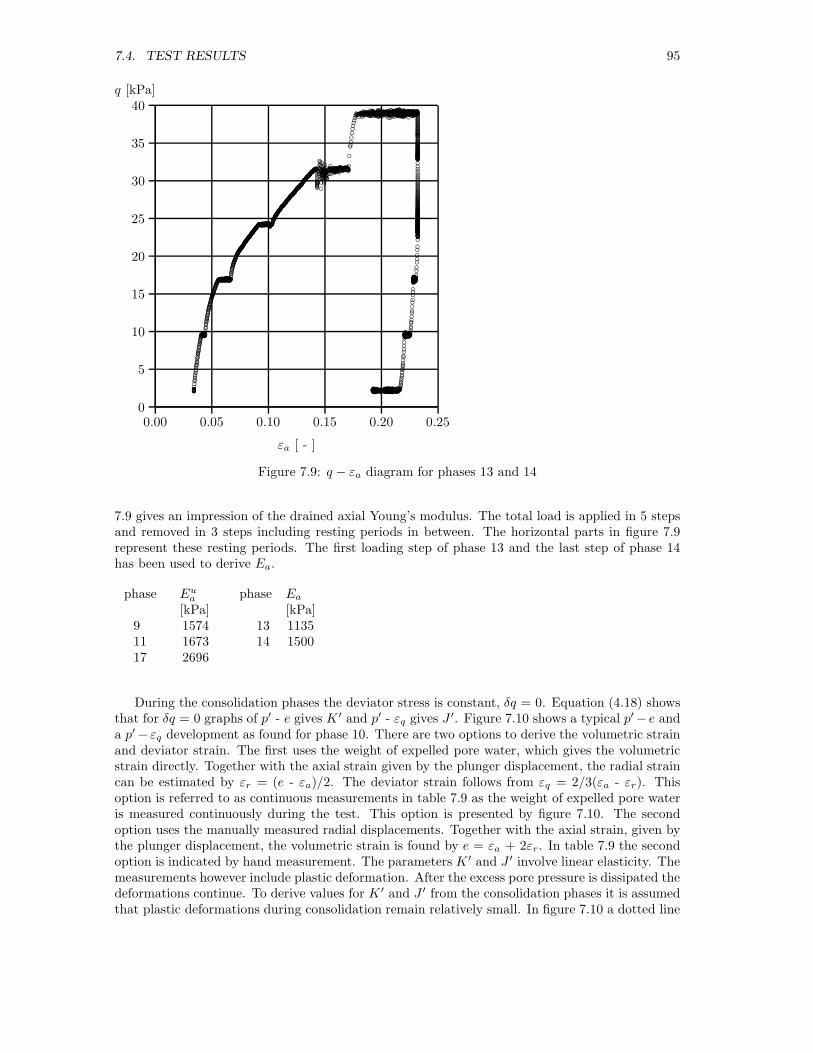
7.4. TEST RESULTS 95
0.00 0.05 0.10 0.15 0.20 0.25
εa [ - ]
0
5
10
15
20
25
30
35
40q [kPa]
◦◦◦◦◦◦◦◦◦◦◦◦◦◦◦◦◦◦◦◦◦◦◦◦◦◦◦◦◦◦◦◦◦◦◦◦◦◦◦◦◦◦◦◦◦◦◦◦◦◦◦◦◦◦◦◦◦◦◦◦◦◦◦◦◦◦◦◦◦◦◦◦◦◦◦◦◦◦◦◦◦◦◦◦◦◦◦◦◦◦◦◦◦◦◦◦◦◦◦◦◦◦◦◦◦◦◦◦◦◦◦◦◦◦◦◦◦◦◦◦◦◦◦◦◦◦◦◦◦◦◦◦◦◦◦◦◦◦◦◦◦◦◦◦◦◦◦◦◦◦◦◦◦◦◦◦◦◦◦◦◦◦◦◦◦◦◦◦◦◦◦◦◦◦◦◦◦◦◦◦◦◦◦◦◦◦◦◦◦◦◦◦◦◦◦◦◦◦◦◦◦◦◦◦◦◦◦◦◦◦◦◦◦◦◦◦◦◦◦◦◦◦◦◦◦◦◦◦◦◦◦◦◦◦◦◦◦◦◦◦◦◦◦◦◦◦◦◦◦◦◦◦◦◦◦◦◦◦◦◦◦◦◦◦◦◦◦◦◦◦◦◦◦◦◦◦◦◦◦◦◦◦◦◦◦◦◦◦◦◦◦◦◦◦◦◦◦◦◦◦◦◦◦◦◦◦◦◦◦◦◦◦◦◦◦◦◦◦◦◦◦◦◦◦◦◦◦◦◦◦◦◦◦◦◦◦◦◦◦◦◦◦◦◦◦◦◦◦◦◦◦◦◦◦◦◦◦◦◦◦◦◦◦◦◦◦◦◦◦◦◦◦◦◦◦◦◦◦◦◦◦◦◦◦◦◦◦◦◦◦◦◦◦◦◦◦◦◦◦◦◦◦◦◦◦◦◦◦◦◦◦◦◦◦◦◦◦◦◦◦◦◦◦◦◦◦◦◦◦◦◦◦◦◦◦◦◦◦◦◦◦◦◦◦◦◦◦◦◦◦◦◦◦◦◦◦◦◦◦◦◦◦◦◦◦◦◦◦◦◦◦◦◦◦◦◦◦◦◦◦◦◦◦◦◦◦◦◦◦◦◦◦◦◦◦◦◦◦◦◦◦◦◦◦◦◦◦◦◦◦◦◦◦◦◦◦◦◦◦◦◦◦◦◦◦◦◦◦◦◦◦◦◦◦◦◦◦◦◦◦◦◦◦◦◦◦◦◦◦◦◦◦◦◦◦◦◦◦◦◦◦◦◦◦◦◦◦◦◦◦◦◦◦◦◦◦◦◦◦◦◦◦◦◦◦
◦◦◦◦◦◦◦◦◦◦◦◦◦◦◦◦◦◦◦◦◦◦◦◦◦◦◦◦◦◦◦◦◦◦◦◦◦◦◦◦◦◦◦◦◦◦◦◦◦◦◦◦◦◦◦◦◦◦◦◦◦◦◦◦◦◦◦◦◦◦◦◦◦◦◦◦◦◦◦◦◦◦◦◦◦◦◦◦◦◦◦◦◦◦◦◦◦◦◦◦◦◦◦◦◦◦◦◦◦◦◦◦◦◦◦◦◦◦◦◦◦◦◦◦◦◦◦◦◦◦◦◦◦◦◦◦◦◦◦◦◦◦◦◦◦◦◦◦◦◦◦◦◦◦◦◦◦◦◦◦◦◦◦◦◦◦◦◦◦◦◦◦◦◦◦◦◦◦◦◦◦◦◦◦◦◦◦◦◦◦◦◦◦◦◦◦◦◦◦◦◦◦◦◦◦◦◦◦◦◦◦◦◦◦◦◦◦◦◦◦◦◦◦◦◦◦◦◦◦◦◦◦◦◦◦◦◦◦◦◦◦◦◦◦◦◦◦◦◦◦◦◦◦◦◦◦◦◦◦
◦◦◦◦◦◦◦◦◦◦◦◦◦◦◦◦◦◦◦◦◦◦◦◦◦◦◦◦◦◦◦◦◦◦◦◦◦◦◦◦◦◦◦◦◦◦◦◦◦◦◦◦◦◦◦◦◦◦◦◦◦◦◦◦◦◦◦◦◦◦◦◦◦◦◦◦◦◦◦◦◦◦◦◦◦◦◦◦◦◦◦◦◦◦◦◦◦◦◦◦◦◦◦◦◦◦◦◦◦◦◦◦◦◦◦◦◦◦◦◦◦◦◦◦◦◦◦◦◦◦◦◦◦◦◦◦◦◦◦◦◦◦◦◦◦◦◦◦◦◦◦◦◦◦◦◦◦◦◦◦◦◦◦◦◦◦◦◦◦◦◦◦◦◦◦◦◦◦◦◦◦◦◦◦◦◦◦◦◦◦◦◦◦◦◦◦◦◦◦◦◦◦◦◦◦◦◦◦◦◦◦◦◦◦◦◦◦◦◦◦◦◦◦◦◦◦◦◦◦◦◦◦◦◦◦◦◦◦◦◦◦◦◦◦◦◦◦◦◦◦◦◦◦
◦◦◦
◦◦◦◦
◦◦◦◦◦◦◦◦◦◦◦◦◦◦◦
◦
◦◦◦◦◦◦◦◦◦◦◦◦◦◦◦◦◦◦◦◦◦◦◦◦◦
◦
◦◦
◦◦◦◦◦◦◦◦◦◦◦◦◦◦◦◦◦◦◦◦◦◦◦◦◦◦◦◦◦◦◦◦◦◦◦◦◦◦◦◦◦◦◦◦◦◦◦◦◦◦◦◦◦◦◦◦◦◦◦◦◦◦◦◦◦◦◦◦◦◦◦◦◦◦◦◦◦◦◦◦◦◦◦◦◦◦◦◦◦◦◦◦◦◦◦◦◦◦◦◦◦◦◦◦◦◦◦◦◦◦◦◦◦◦◦◦◦◦◦◦◦◦◦◦◦◦◦◦◦◦◦◦◦◦◦◦◦◦◦◦◦◦◦◦◦◦◦◦◦◦◦◦◦◦◦◦◦◦◦◦◦◦◦◦◦◦◦◦◦◦◦◦◦◦◦◦◦◦◦◦◦◦◦◦◦◦◦◦◦◦◦◦◦◦◦◦◦◦◦◦◦◦◦◦
◦
◦◦◦◦◦◦◦◦◦◦◦◦◦◦◦◦◦◦◦◦◦◦◦◦◦◦◦◦◦◦◦◦◦◦◦◦◦◦◦◦◦◦◦◦◦◦◦◦◦◦◦◦◦◦◦◦◦◦◦◦◦◦◦◦◦◦◦◦◦◦◦◦◦◦◦◦◦◦◦◦◦◦◦◦◦◦◦◦◦◦◦◦◦◦◦◦◦◦◦◦◦◦◦◦◦◦◦◦◦◦◦◦◦◦◦◦◦◦◦◦◦◦◦◦◦◦◦◦◦◦◦◦◦◦◦◦◦◦◦◦◦◦◦◦◦◦◦◦◦◦◦◦◦◦◦◦◦◦◦◦◦◦◦◦◦◦◦◦◦◦◦◦◦◦◦◦◦◦◦◦◦◦◦◦◦◦◦◦◦◦◦◦◦◦◦◦◦◦◦◦◦◦◦◦◦◦◦◦◦◦◦◦◦◦◦◦◦◦◦◦◦◦◦◦◦◦◦◦◦◦◦◦◦◦◦◦◦◦◦◦◦◦◦◦◦◦◦◦◦◦◦◦◦◦◦◦◦◦◦◦◦◦◦◦◦◦◦◦◦◦◦◦◦◦◦◦◦◦◦◦◦◦◦◦◦◦◦◦◦◦◦◦◦◦◦◦◦◦◦◦◦◦◦◦◦◦◦◦◦◦◦◦◦◦◦◦◦◦◦◦◦◦◦◦◦◦◦◦◦◦◦◦◦◦◦◦◦◦◦◦◦◦◦◦◦◦◦◦◦◦◦◦◦◦◦◦◦◦◦◦◦◦◦◦◦◦◦◦◦◦◦◦◦◦◦◦◦◦◦◦◦◦◦◦◦◦◦◦◦◦◦◦◦◦◦◦◦◦◦◦◦◦◦◦◦◦◦◦◦◦◦◦◦◦◦◦◦◦◦◦◦◦◦◦◦◦◦◦◦◦◦◦◦◦◦◦◦◦◦◦◦◦◦◦◦◦◦◦◦◦◦◦◦◦◦◦◦◦◦◦◦◦◦◦◦◦◦◦◦◦◦◦◦◦◦◦◦◦◦◦◦◦◦◦◦◦◦◦◦◦◦◦◦◦◦◦◦◦◦◦◦◦◦◦◦◦◦◦◦◦◦◦◦◦◦◦◦◦◦◦◦◦◦◦◦◦◦◦◦◦◦◦◦◦◦◦◦◦◦◦◦◦◦◦◦◦◦◦◦◦◦◦◦◦◦◦◦◦◦◦◦◦◦◦◦◦◦◦◦◦◦◦◦◦◦◦◦◦◦◦◦◦◦◦◦◦◦◦◦◦◦◦◦◦◦◦◦◦◦◦◦◦◦◦◦◦◦◦◦◦◦◦◦◦◦◦◦◦◦◦◦◦◦◦◦◦◦◦◦◦◦◦◦◦◦◦◦◦◦◦◦◦◦◦◦◦◦◦◦◦◦◦◦◦◦◦◦◦◦◦◦◦◦◦◦◦◦◦◦◦◦◦◦◦◦◦◦◦◦◦◦◦◦◦◦◦◦◦◦◦◦◦◦◦◦◦◦◦◦◦◦◦◦◦◦◦◦◦◦◦◦◦◦◦◦◦◦◦◦◦◦◦◦◦◦◦◦◦◦◦◦◦◦◦◦◦◦◦◦◦◦◦◦◦◦◦◦◦◦◦◦◦◦◦◦◦◦◦◦◦◦◦◦◦◦◦◦◦◦◦◦◦◦◦◦◦◦◦◦◦◦◦◦◦◦◦◦◦◦◦◦◦◦◦◦◦◦◦◦◦◦◦◦◦◦◦◦◦◦◦◦◦◦◦◦◦◦◦◦◦◦◦◦◦◦◦◦◦◦◦◦◦◦◦◦◦◦◦◦◦◦◦◦◦◦◦◦◦◦◦◦◦◦◦◦◦◦◦◦◦◦◦◦◦◦◦◦◦◦◦◦◦◦◦◦◦◦◦◦◦◦◦◦◦◦◦◦◦◦◦◦◦◦◦◦◦◦◦◦◦◦◦◦◦◦◦◦◦◦◦◦◦◦◦◦◦◦◦◦◦◦◦◦◦◦◦◦◦◦◦◦◦◦◦◦◦◦◦◦◦◦◦◦◦◦◦◦◦◦◦◦◦◦◦◦◦◦◦◦◦◦◦◦◦◦◦◦◦◦◦◦◦◦◦◦◦◦◦◦◦◦◦◦◦◦◦◦◦◦◦◦◦◦◦◦◦◦◦◦◦◦◦◦◦◦◦◦◦◦◦◦◦◦◦◦◦◦◦◦◦◦◦◦◦◦◦◦◦◦◦◦◦◦◦◦◦◦◦◦◦◦◦◦◦◦◦◦◦◦◦◦◦◦◦◦◦◦◦◦◦◦◦◦◦◦◦◦◦◦◦◦◦◦◦◦◦◦◦◦◦◦◦◦◦◦◦◦◦◦◦◦◦◦◦◦◦◦◦◦◦◦◦◦◦◦◦◦◦◦◦◦◦◦◦◦◦◦◦◦◦◦◦◦◦◦◦◦◦◦◦◦◦◦◦◦◦◦◦◦◦◦◦◦◦◦◦◦◦◦◦◦◦◦◦◦◦◦◦◦◦◦◦◦◦◦◦◦◦◦◦◦◦◦◦◦◦◦◦◦◦◦◦◦◦◦◦◦◦◦◦◦◦◦◦◦◦◦◦◦◦◦◦◦◦◦◦◦◦◦◦◦◦◦◦◦◦◦◦◦◦◦◦◦◦◦◦◦◦◦◦◦◦◦◦◦◦◦◦◦◦◦◦◦◦◦◦◦◦◦◦◦◦◦◦◦◦◦◦◦◦◦◦◦◦◦◦◦◦◦◦◦◦◦◦◦◦◦◦◦◦◦◦◦◦◦◦◦◦◦◦◦◦◦◦◦◦◦◦◦◦◦◦◦◦◦◦◦◦◦◦◦◦◦◦◦◦◦◦◦◦◦◦◦◦◦◦◦◦◦◦◦◦◦◦◦◦◦◦◦◦◦◦◦◦◦◦◦◦◦◦◦◦◦◦◦◦◦◦◦◦◦◦◦◦◦◦◦◦◦◦◦◦◦◦◦◦◦◦◦◦◦◦◦◦◦◦◦◦◦◦◦◦◦◦◦◦◦◦◦◦◦◦◦◦◦◦◦◦◦◦◦◦◦◦◦◦◦◦◦◦◦◦◦◦◦◦◦◦◦◦◦◦◦◦◦◦◦◦◦◦◦◦◦◦◦◦◦◦◦◦◦◦◦◦◦◦◦◦◦◦◦◦◦◦◦◦◦◦◦◦◦◦◦◦◦◦◦◦◦◦◦◦◦◦◦◦◦◦◦◦◦◦◦◦◦◦◦◦◦◦◦◦◦◦◦◦◦◦◦◦◦◦◦◦◦◦◦◦◦◦◦◦◦◦◦◦◦◦◦◦◦◦◦◦◦◦◦◦◦◦◦◦◦◦◦◦◦◦◦◦◦◦◦◦◦◦◦◦◦◦◦◦◦◦◦◦◦◦◦◦◦◦◦◦◦◦◦◦◦◦◦◦◦◦◦◦◦◦◦◦◦◦◦◦◦◦◦◦◦◦
◦◦◦◦◦◦◦◦◦◦◦◦◦◦◦◦◦◦◦◦◦◦◦◦◦◦◦◦◦◦◦◦◦◦◦◦◦◦◦◦◦◦◦◦◦◦◦◦◦◦◦◦◦◦◦◦◦◦◦◦◦◦◦◦◦◦◦◦◦◦◦◦◦◦◦◦◦◦◦◦◦◦◦◦◦◦◦◦◦◦◦◦◦◦◦◦◦◦◦◦◦◦◦◦◦◦◦◦◦◦◦◦◦◦◦◦◦◦◦◦◦◦◦◦◦◦◦◦◦◦◦◦◦◦◦◦◦◦◦◦◦◦◦◦◦◦◦◦◦◦◦◦◦◦◦◦◦◦◦◦◦◦◦◦◦◦◦◦◦◦◦◦◦◦◦◦◦◦◦◦◦◦◦◦◦◦◦◦◦◦◦◦◦◦◦◦◦◦◦◦◦◦◦◦◦◦◦◦◦◦◦◦◦◦◦◦◦◦◦◦◦◦◦◦◦◦◦◦◦◦◦◦◦◦◦◦◦◦◦◦◦◦◦◦◦◦◦◦◦◦◦◦◦◦◦◦◦◦◦◦◦◦◦◦◦◦◦◦◦◦◦◦◦◦◦◦◦◦◦◦◦◦◦◦◦◦◦◦◦◦◦◦◦◦◦◦◦◦◦◦◦◦◦◦◦◦◦◦◦◦◦◦◦◦◦◦◦◦◦◦◦◦◦◦◦◦◦◦◦◦◦◦◦◦◦◦◦◦◦◦◦◦◦◦◦◦◦◦◦◦◦◦◦◦◦◦◦◦◦◦◦◦◦◦◦◦◦◦◦◦◦◦◦◦◦◦◦◦◦◦◦◦◦◦◦◦◦◦◦◦◦◦◦◦◦◦◦◦◦◦◦◦◦◦◦◦◦◦◦◦◦◦◦◦◦◦◦◦◦◦◦◦◦◦◦◦◦◦◦◦◦◦◦◦◦◦◦◦◦◦◦◦◦◦◦◦◦◦◦◦◦◦◦◦◦◦◦◦◦◦◦◦◦◦◦◦◦◦◦◦◦◦◦◦◦◦◦◦◦◦◦◦◦◦◦◦◦◦◦◦◦◦◦◦◦◦◦◦◦◦◦◦◦◦◦◦◦◦◦◦◦◦◦◦◦◦◦◦◦◦◦◦◦◦◦◦◦◦◦◦◦◦◦◦◦◦◦◦◦◦◦◦◦◦◦◦◦◦◦◦◦◦◦◦◦◦◦◦◦◦◦◦◦◦◦◦◦◦◦◦◦◦◦◦◦◦◦◦◦◦◦◦◦◦◦◦◦◦◦◦◦◦◦◦◦◦◦◦◦◦◦◦◦◦◦◦◦◦◦◦◦◦◦◦◦◦◦◦◦◦◦◦◦◦◦◦◦◦◦◦◦◦◦◦◦◦◦◦◦◦◦◦◦◦◦◦◦◦◦◦◦◦◦◦◦◦◦◦◦◦◦◦◦◦◦◦◦◦◦◦◦◦◦◦◦◦◦◦◦◦◦◦◦◦◦◦◦◦◦◦◦◦◦◦◦◦◦◦◦◦◦◦◦◦◦◦◦◦◦◦◦◦◦◦◦◦◦◦◦◦◦◦◦◦◦◦◦◦◦◦◦◦◦◦◦◦◦◦◦◦◦◦◦◦◦◦◦◦◦◦◦◦◦◦◦◦
◦◦◦◦◦◦◦◦◦◦◦◦◦◦◦◦◦◦◦◦◦◦◦◦◦◦
Figure 7.9: q − εa diagram for phases 13 and 14
7.9 gives an impression of the drained axial Young’s modulus. The total load is applied in 5 stepsand removed in 3 steps including resting periods in between. The horizontal parts in figure 7.9represent these resting periods. The first loading step of phase 13 and the last step of phase 14has been used to derive Ea.
phase Eua phase Ea[kPa] [kPa]
9 1574 13 113511 1673 14 150017 2696
During the consolidation phases the deviator stress is constant, δq = 0. Equation (4.18) showsthat for δq = 0 graphs of p′ - e gives K ′ and p′ - εq gives J ′. Figure 7.10 shows a typical p′− e anda p′− εq development as found for phase 10. There are two options to derive the volumetric strainand deviator strain. The first uses the weight of expelled pore water, which gives the volumetricstrain directly. Together with the axial strain given by the plunger displacement, the radial straincan be estimated by εr = (e - εa)/2. The deviator strain follows from εq = 2/3(εa - εr). Thisoption is referred to as continuous measurements in table 7.9 as the weight of expelled pore wateris measured continuously during the test. This option is presented by figure 7.10. The secondoption uses the manually measured radial displacements. Together with the axial strain, given bythe plunger displacement, the volumetric strain is found by e = εa + 2εr. In table 7.9 the secondoption is indicated by hand measurement. The parameters K ′ and J ′ involve linear elasticity. Themeasurements however include plastic deformation. After the excess pore pressure is dissipated thedeformations continue. To derive values for K ′ and J ′ from the consolidation phases it is assumedthat plastic deformations during consolidation remain relatively small. In figure 7.10 a dotted line

96 CHAPTER 7. LARGE SCALE TRIAXIAL TEST
indicates the end of consolidation, which often corresponds to a strong curvature at the end of theconsolidation period.
4 6 8 10 12 14
p′ [kPa]
−0.010
−0.008
−0.006
−0.004
−0.002
0.000
0.002
e [ - ]
εq [ - ]
.............
.............
.............
.............
.............
.............
.............
.............
.............
.............
.............
.............
.............
.............
......
p′ − εq
p′ − e
•
•••••••••••••••••
••••••••••••••••••••••••••••••••••••••••••••
••••••••••••••••••••••••
•••••••••••••••••••••••••••••••••••••••••••••••••••••••••••••••••••••••••••••••••••••••••••••••••••••••••••••••••••••••••••••••
∗∗∗∗∗∗∗∗∗∗∗∗∗∗∗∗∗∗∗∗∗∗∗∗∗∗∗∗∗∗∗∗∗∗∗∗∗∗∗∗∗∗∗∗∗∗∗∗∗∗∗∗∗∗∗∗∗∗∗∗∗∗∗∗∗∗∗∗∗∗∗∗∗∗∗∗∗∗∗∗∗∗∗∗∗∗∗∗∗∗∗∗∗∗∗∗∗∗∗∗∗∗∗∗∗∗∗∗∗∗∗∗∗∗∗∗∗∗∗∗∗∗∗∗∗∗∗∗∗∗∗∗∗∗∗∗∗∗∗∗∗∗∗∗∗∗∗∗∗∗∗∗∗∗∗∗∗∗∗∗∗∗∗∗∗∗∗∗∗∗∗∗∗∗∗∗∗∗∗∗∗∗∗∗∗∗∗∗∗∗∗∗∗∗∗∗∗∗∗∗∗∗∗∗∗∗∗∗∗∗∗∗∗
Figure 7.10: p′ − e and p′ − εq development for phase 10
Table 7.9 gives the values for K ′, J ′ and K ′/J ′ found for the different consolidation phases.The phases 6, 8 and 16 gives the consolidation under an isotropic load, while the phases 10, 12and 18 gives the consolidation under an axial stress.
Table 7.9 shows for phases 6, 8 and 10 equivalent results of both methods. For the phases 12,16 and 18 large difference occur especially in determination of J ′. Due to the axial deformationsthe membrane around the sample starts to buckle and curl. Since the total radial displacementsare very small, buckling of the membrane induces a relatively large error. This explains that in thefinal phases the manual measurements indicate a larger volumetric strain and a smaller deviatorstrain than found by the continuous measurements
Table 7.9: Stiffness moduli K ′ and J ′ derived from the consolidation phasesphase continuous hand measurements
K ′ J ′ K ′/J ′ K ′ J ′ K ′/J ′
[kPa] [kPa] [ - ] [kPa] [kPa] [ - ]6 407 2010 0.20 452 1943 0.238 645 1800 0.36 898 1400 0.6310 389 1094 0.36 407 935 0.4412 484 1770 0.27 255 7837 0.0316 530 1709 0.31 350 4443 0.0818 730 - 670∗ 1450-1550∗ 0.50-0.40∗ 407 1207 0.13∗ due to measurement noise an exact value can not be given
Table 7.9 shows a scatter in values found for K ′ and J ′. The values for K ′/J ′ are moreconsistent than the values derived by the hand held laser.

7.5. FITTING MEASUREMENT DATA 97
7.5 Fitting measurement data
During the consolidation phases 16 and 18 a clear Mandel–Cryer effect is found. Figure 7.11 showsa comparison between measurement data and analytical solution presented by chapter 5. Theradial strain is found to be small, as shown by table 7.8. The ratio of the radial strain and theaxial strain found in the drained unloading phase 13 gives an estimation of νvh, νvh ≈ 0.1. Theprevious section shows that the axial drained Young’s modulus of the order of 1200 - 1500 kPa.Under the assumption νhh ≈ νvh, this leaves the permeability and the radial drained Young’smodulus to fit the analytical solution to the measurement data. The following parameters arefound:
phase 16 phase 18Ea 1200 kPa 1200 kPaEr 3300 kPa 3300 kPaνvh 0.1 0.1νhh 0 0.1(K ′/J ′ 0.27 0.3)k 8 × 0−8 m/s 6 × 10⁻⁸ m/s
0.1 1 10 102 103 104
t [s]
−0.2
0.0
0.2
0.4
0.6
0.8
1.0
1.2
1.4
1.6σw/σb
◦
∗
phase 18
phase 16
◦ ◦◦ ◦
◦◦◦
◦◦◦◦◦
◦◦◦◦◦◦◦◦◦◦◦
◦◦◦◦◦◦◦◦◦◦◦◦◦◦◦◦◦◦◦◦◦◦◦◦◦◦◦◦◦◦◦◦◦◦◦◦◦◦◦◦◦◦◦◦◦◦◦◦◦◦◦◦◦◦◦◦◦◦◦◦◦◦◦◦◦◦◦◦◦◦◦◦◦◦◦◦◦◦◦◦◦◦◦◦◦◦◦◦◦◦◦◦◦◦◦◦◦◦◦◦◦◦◦◦◦◦◦◦◦◦◦◦◦◦◦◦◦◦◦◦◦◦◦◦◦◦◦◦◦◦◦◦◦◦◦◦◦◦◦◦◦◦◦◦◦◦◦◦◦◦◦◦◦◦◦◦◦◦◦◦◦◦◦◦◦◦◦◦◦◦◦◦◦◦◦◦◦◦◦◦◦◦◦◦◦◦◦◦◦◦◦◦◦◦◦◦◦◦◦◦◦◦◦◦◦◦◦◦◦◦◦◦◦◦◦◦◦◦◦◦◦◦◦◦◦◦◦◦◦◦◦◦◦◦◦◦◦◦◦◦◦◦◦◦◦◦◦◦◦◦◦◦◦◦◦◦◦◦◦◦◦◦◦◦◦◦◦◦◦◦◦◦◦◦◦◦◦◦◦◦◦◦◦◦◦◦◦◦◦◦◦◦◦◦◦◦◦◦◦◦◦◦◦◦◦◦◦◦◦◦◦◦◦◦◦◦◦◦◦◦◦◦◦◦◦◦◦◦◦◦◦◦◦◦◦◦◦◦◦◦◦◦◦◦◦◦◦◦◦◦◦◦◦◦◦◦◦◦◦◦◦◦◦◦◦◦◦◦◦◦◦◦◦◦◦◦◦◦◦◦◦◦◦◦◦◦◦◦◦◦◦◦◦◦◦◦◦◦◦◦◦◦◦◦◦◦◦◦◦◦◦◦◦◦◦◦◦◦◦◦◦◦◦◦◦◦◦◦◦◦◦◦◦◦◦◦◦◦◦◦◦◦◦◦◦◦◦◦◦◦◦◦◦◦◦◦◦◦◦◦◦◦◦◦
∗
∗
∗
∗
∗∗∗∗
∗∗∗∗∗∗∗∗∗∗∗∗∗∗
∗∗∗∗∗∗∗∗∗∗∗∗∗∗∗∗∗∗∗∗∗∗∗∗∗∗∗∗∗∗∗∗∗∗∗∗∗∗∗∗∗∗∗∗∗∗∗∗∗∗∗∗∗∗∗∗∗∗∗∗∗∗∗∗∗∗∗∗∗∗∗∗∗∗∗∗∗∗∗∗∗∗∗∗∗∗∗∗∗∗∗∗∗∗∗∗∗∗∗∗∗∗∗∗∗∗∗∗∗∗∗∗∗∗∗∗∗∗∗∗∗∗∗∗∗∗∗∗∗∗∗∗∗∗∗∗∗
∗∗∗∗∗∗∗∗∗∗∗∗∗∗∗∗∗∗∗∗∗∗∗∗∗∗∗∗∗∗∗∗∗∗∗∗∗∗∗∗∗∗∗∗∗∗∗∗∗∗∗∗∗∗∗∗∗∗∗∗∗∗∗∗∗∗∗∗∗∗∗∗∗∗∗∗∗∗∗∗∗∗∗∗∗
..............................................................................................................................................................................................................................
...........................................................................
.................................................
................................
..............................................................................................
................................................................................................................................................................................................................................................................................................................................................................................
................................................................................................................................................................................................
.........................................................................
...............................................
....................................
...........................
...........................................................................................................................................................................................................................................................................................................................................................................................................................................................................................................................................................................................
Figure 7.11: Analytical fit for measurement data phases 16 and 18
Figure 7.6 shows the pore pressure development for two axial loading phases 10 and 18 and oneaxial unloading phase, phase 12. The initial pore pressure in relation to the applied load, σb inphases 10 and 12 is in the same order of magnitude as phase 18. However as consolidation proceedsthe pore pressure development shows a lower peak and a less steep slope for phases 10 and 12. Thepore pressure development found in these phases can not be reproduced by the analytical formulaeof chapter 5. The stiffness parameters which reproduce the initial pore pressure will predict alarger peak and vice–versa.
Section 6.7.2 explains the absence of a large Mandel–Cryer effect for the conventional triaxialtesting by drain resistance. However the absence of a large peak in the phase 6, 8, 10 and 12 forlarge scale testing can not be explained by drain resistance. First, measurements of drain pressure,pd, show that after opening the valves the drain pressure adjust almost instantaneously to thepressure in the pore water collection system. This indicates that ∆pd = 0, at least at the ends

98 CHAPTER 7. LARGE SCALE TRIAXIAL TEST
of the drains. Second, a nice fit of measurement data can be found for the phases 16 and 18disregarding drain resistance. Drain resistance is independent from loading phases. So if duringphases 16 and 18 drain resistance does not influence the pore pressure development then drainresistance does not influence the pore pressure developments in the other phases.
Gibson, Gobert & Schiffmann [33] show that a non–constant permeability leads to a reductionin the Mandel–Cryer effect in combination to an increase in hydrodynamic period. The increasein hydrodynamic period is repeated by a flattening of the consolidation curve. A non constantpermeability might explain the differences between the analytical solution and measurement datafor phases 10 and 12.
Section 6.2.3 shows the strain dependency of the permeability of the peat used for the conven-tional triaxial samples. Equivalent to section 6.2.3 strain dependency is determined for the materialtested in the large scale triaxial test. K0 − CRS tests are conducted on conventional samples re-trieved in the vicinity of location where the large sample has been retrieved. The measurementsare used to fit equation (7.1)
k = k0 × exp (−χe) (7.1)
In total 10 samples have been tested. On average is found χ = 8.5 and k0 = 4.5 ×10⁻⁸ m/s.Based on strain measurement equation (7.1) is used to calculate the actual permeability at the beginand end of the different consolidation phases. Equation (7.1) relates permeability to volumetricstrain. Since k0 refers to initial conditions the total volumetric strain is needed to find a propervalue for the actual permeability. Section 7.4.2 shows that volumetric strain measurement in initialphases of the test is not trustworthy. Therefore an accurate development of the permeability duringthe test can not be given. Table 7.8 shows that the radial strain is small in comparison to the axialstrain. To illustrate the development of the permeability figure 7.12 uses the total axial strain incombination to equation (7.1).
0.00 0.05 0.10 0.15 0.20 0.25
εa [ - ]
0.0
0.5
1.0
1.5
2.0
2.5
3.0
3.5
4.0
4.5
5.0
k × 10−8 [m/s]
...............................
......................................
............. ...................
•
•∗∗⋄⋄◦◦
××△△
•
∗
⋄
◦
×
△
phase 6
phase 8
phase 10
phase 12
phase 16
phase 18
Figure 7.12: Illustration of decay in permeability during the test, based on axial strain
Figure 7.12 shows the decay in permeability when strain develops. It should be noted that theactual value for k used in figure 7.11 to fit the measurement data is larger than presented in thisfigure. Figure 7.12 clearly shows that the permeability decays strongly within the phases 6, 8, 10and 12. After the large axial pre–consolidation the permeability is reduced by almost an order inmagnitude. However during the phases 16 and 18 the change in permeability is small to negligible.This indicates that for the phase 6, 8, 10 and 12 the variability of the permeability might maskthe Mandel–Cryer effect. While for the phases 16 and 18 a peak is found conform the analyticalsolution presented in chapter 5.

7.6. CONCLUSIONS 99
7.6 Conclusions
Section 7.1 discusses the aim of the large scale triaxial test, which is to study possible scale effects.Two possible scale effects are explicitly mentioned. First in relation to the Mandel–Cryer effect.Second in relation to the influence of an axial pre–consolidation.
Regarding the Mandel–Cryer it can be concluded that the measurements on the large scaletriaxial test show the Mandel–Cryer effect in contrast to the conventional samples presented insection 6.7. The Mandel–Cryer effect is found during consolidation after an axial load as well asafter an isotropic load. A small Mandel–Cryer effect is found for the non pre–consolidated phasesand large effects are found for the axial pre–consolidated phase. The large effects can well befitted to the analytical solutions presented in chapter 5. The small effects found in the non pre–consolidated phases can be explained by a non constant permeability. According to equation (7.1)a significant change in permeability is to be expected during the non pre–consolidated phases whilefor the pre–consolidated phases the change in permeability is relatively small. This is illustratedby figure 7.12. A variable permeability is also found for the peat tested in the conventional triaxialtests, see table 6.2. It is therefore concluded that absence of the Mandel–Cryer effect in theconventional triaxial tests can be explained by drain resistance in combination with a non-constantpermeability. For large sample sizes the Mandel–Cryer effect is more pronounced.
To estimate the influence of an axial pre–consolidation the parameter K ′/J ′ in different ways atdifferent stages of the test. Table 7.10 compares the different values found for the different phases.
Table 7.10: Summary of K ′/J ′ values found in different phases of the testphase ∆p′/∆q (∆σw/∆σb)ini equation 3.2
table 7.6 table 7.5 table 7.96 - - 0.208 - - 0.369 0.35 - -10 - 0.25 0.3611 0.38 - -12 - 0.15 0.2716 - - 0.3117 0.52 - -18 - 0.30 0.50-0.40
Despite the difference in K ′/J ′ value found table 7.10 shows clearly the anisotropy of peat.For all phases the K ′/J ′ value is larger than 0. Table 7.10 shows the different values for K ′/J ′ inthe range of 0.15 to 0.50. The large value 0.52 is found from the angle undrained ESP, which isinfluenced by internal consolidation during application of the load. Therefore it can be concludedthat the angle of undrained ESP is not an appropriate parameter to indicate anisotropy for largescale testing. In contrast to the tests on conventional samples, as shown by the previous chapter,the axial pre–consolidation seems to have a limited influence on the K ′/J ′ value. The K ′/J ′ valueis already considerable for the non pre–consolidated phases. This can be explained by a possibleaxial pre–consolidation in the field, which causes a large value for K ′/J ′ for the phases 6 to 12.The sample was retrieved from a secondary dyke and it will have been axially pre–loaded.
The tested sample is retrieved such that the axial direction corresponds to the vertical directionin the field. However due to the applied loading and unloading phases the stiffness parametersderived from the test hold only for the tested sample and will probably not correspond to theoriginal stiffness parameters in the field. Therefore the stiffness parameters are discussed in termsof Er and Ea of the sample and not in terms of Eh and Ev in the field. To give an impressionof the consequences for the values found for K ′/J ′, equation 3.6 and table 7.11 are used to give arough estimation for the radial stiffness. For three characteristic values for K ′/J ′ from table 7.10

100 CHAPTER 7. LARGE SCALE TRIAXIAL TEST
a value for Er is estimated. The largest value for K ′/J ′ is found in phase 17 and equals 0.52, thelowest value for K ′/J ′ equals 0.15 and an intermediate value of K ′/J ′ = 0.35. The values for thedrained parameters Ea and νvh are derived from phase 13, Ea = 1200 kPa and νvh = 0.1. For νhhthe values 0 and 1/3 are used to estimate Er.
Table 7.11: A rough estimation for Er from measurements of K ′/J ′ and Eaphase Ea K ′/J ′ νvh νhh Er
[kPa] [ - ] [ - ] [ - ] [kPa]12 1200 0.15 0.1 0 2275
1/3 15209 1200 0.35 0.1 0 4210
1/3 280011 1200 0.52 0.1 0 7110
1/3 4750
Table 7.11 shows large values for Er. It should be noted that the radial stiffness follows fromradial deformations due to axial loading. The fibre structure of peat is such that an axial loadleads mainly to axial deformation while radial deformation remains negligible. Therefore large toextreme values for Er are found.
Chapter 8
Practical applications
8.1 Theory, Measurements and Engineering Practice
The chapters 3 to 7 give an answer to the question raised in chapter 1: Can redistribution ofstresses during consolidation of a triaxial sample be used to determine elastic stiffness parameters?In chapter 1 it is notified that soil behaviour is not elastic. However chapter 1 states that equivalentelastic moduli, which incorporate a small amount of plasticity, can be used to describe stress andstrain in soft soil for a large number of consolidation problems. The theory for linear elasticconsolidation is further elaborated in the chapters 3 to 5. The theory is tested by laboratorymeasurements described in chapter 6 and 7. In this chapter theoretical considerations and resultsof the laboratory measurements are linked to engineering practice.
The practical applications of the theory described in chapters 3 to 5 and the conclusions of thelaboratory measurements are illustrated by 3 examples, which are discussed in the next sections;
1 Parameter determination for anisotropy. The initial aim of this study is to find anisotropicparameters by using measurements of pore pressure development in standard triaxial testing.Section 8.2 shows an example in which the level of anisotropy can be distinguished fromstandard laboratory tests.
2 Lateral stress reaction. The laboratory tests described in section 6.6 show a change in levelof anisotropy due to anisotropic pre–loading. A change in ratio of stiffness parameters willlead to a different deformation pattern if such a pre–loaded sample is loaded and allowedto deform. When such pre–loaded sample is not allowed to deform laterally a change instiffness parameters will lead to different lateral stress reaction when the sample is axiallyloaded. Section 8.3 deals with this topic by discussing the influence of anisotropy to theK0-value. This section also shows indicatively the influence of plasticity to the developmentof an anisotropic K0.
3 Consolidation around a vertical drain. In practice vertical drains are often used to improvethe consolidation behaviour of soft soil. Section 8.4 discusses the influence of anisotropy onthe efficiency of vertical drains.
8.2 Parameter determination for anisotropy
Chapter 6 shows that for standard triaxial testing the Mandel–Cryer effect cannot be used todetermine the level of anisotropy for peat in standard triaxial testing. This is caused by drainresistance in combination to a short hydrodynamic period for a radial drained triaxial sample.Chapter 7 shows that besides drain resistance and scale effects a variable permeability influences
101

102 CHAPTER 8. PRACTICAL APPLICATIONS
the Mandel–Cryer effect strongly. For a variable permeability only a small to negligible Mandel–Cryer effect is found. Since variability in permeability in peat can only be excluded from testsafter remoulding the sample severely, measurements of the Mandel–Cryer effect cannot be used toassess the level of anisotropy of peat.
Chapter 6 however shows an increase in angle of undrained effective stress path for axial pre–consolidation indicating an increase in anisotropy. So anisotropy in stiffness can be used for abetter understanding of undrained ESP’s for over–consolidated peat samples. This is illustratedby a series of triaxial tests run on peat samples retrieved underneath the dike around the Islandof Marken. Figure 8.1 shows the results for 12 tests for OCR ≈ 2. The tests have been conductedin order to study dike stability. Six samples have been retrieved from the toe of the dike andtherefore consolidated at a low pressure, approximately 10 kPa. The other six have been retrievedfrom underneath the dike and are therefore consolidated at a higher pressure, approximately 30-40kPa. The water content W density, ρ and loss on ignition N are derived from remaining soilsamples. On average is found a water content W = 7.64 and a density ρ = 982 kg/m3 for thesamples at the toe of the dike. For the samples collected underneath the dike is found W = 5.03 andρ = 1008 kg/m3. On average N = 0.80 is found. These values correspond well to values presentedin literature, [25]. Figure 8.1 shows that all the stress paths are tilting backwards, except fromtest nr 167, until failure occurs.
For large values of q the horizontal effective stress reduces to 0 due to the pore pressure genera-tion. The samples consolidated at a low pressure fail when reaching these conditions. The samplesconsolidated at large pressure do not fail when the horizontal stress reduces to 0. For these teststhe ESP follows the line q = 3p′ which follow directly from the definitions of p′ and q.
The upper part of figure 8.1 presents the ESP’s for each test. The lower part shows thecorresponding q–εa curve. As a reference the p′–q combination when εa reaches 2 % is indicatedin figure 8.1 by the symbol +. The tests are ended when εa = 15 % is reached. Table 8.1 gives theangle in undrained ESP. The angle of ESP is found by application of the least squares method tothe range of q = 0 to 4 kPa.
Table 8.1: The ∆p′/∆q value, between brackets the average values without test 167at toe of dike underneath the diketest nr ∆p′/∆q test nr ∆p′/∆q102 -0.18 47 -0.25167 0.06 57 -0.32135 -0.11 78 -0.29160 -0.22 85 -0.21175 -0.27 86 -0.24152 -0.15 96 -0.34average -0.15 -0.28
(-0.19)
Table 8.1 shows a clear difference in ∆p′/∆q values for samples at the toe of the dike andunderneath the dike. Soil investigation on the island of Marken shows that the peat layer isapproximately 3.5 m thick at the toe of the dike, while underneath the dike the thickness isreduced to 2.1 m. This suggests that the weight of the dike has compressed the peat layer byapproximately 40 %. This is of the same order in magnitude as used for the pre–consolidation insection 6.6.2.
The compression of the peat layer underneath the dike is also found in the actual values for Wand ρ. As mentioned before a lower value or W is found underneath the dike, W = 5.03, than atthe toe of the dike, W = 7.64. With W = ρwn/ρs(1 − n), the difference in W might indicate apore volume reduction of approximately 35 %. This corresponds well to the global observation ofa 40 % reduction in peat layer thickness. The difference in density also suggests a compression of

8.2. PARAMETER DETERMINATION FOR ANISOTROPY 103
0 10 20 30 40 50
p′ [kPa]
0
10
20
30
40
50
60
70
80
90p′ = 3q
q [kPa]
................................................................................................................................................................................................................................................................................................................................................................................................................................................................................................................................................................................................................................................................................................................
++++
+++
+
++ +
+
+
+ ǫa = 2%
....
....................................................................................................
...
...
...
...
...
...
...
...
...
...
...
...
...
.....................................
......
.....
.
.....
...................................................................
.........................................
..
.
..........
...
......
.....
........
.................
...........
...................................................................................................................................................................................................................................................................................................................................................................................................................................................................................................
.........................................................
...................................................................................................................................................................................................................................................................................................
........................
..................
............
............
............
........................
............
............
............
..................
............
..................................................................................................................................................................
........................................................................................................................................................................................................
..................
...
.................
.........
..............................................................................
........
....
.....................................................................
0 5 10 15 20 25
ǫa [%]
0
10
20
30
40
50
60
70
80
90
q [kPa]
toe of
dike
underneath
dike
....................................................................................................
...............................
.............................................
................................................
.................................................................................
................................................................................................................................................................
............................................................................................ test 102
....................................................................................
..................
........................
................................
.............................................................................................................
..................................................................... test 167
....................................................................................
........................
...................................
...............................
......................................
...............................................
...................................................................... test 135
..............................................
.............
........................
......................................................................................
.............................
.............................................. test 160
.......................
......
..........
.....................
...........................................
.......
....................... test 175
.................
.. .. . .
. . . .. . . .
. . . . .. . . . . . . . . .
. . . . . . . . . . . . . . . . . .. . . . . . . . . . . . . . . . test 152
................
.......
.....
......
.....
....
.....
....
....
....
.....
....
....
......
....
....
....
....
....
....
....
....
....
....
....
.....
....
....
....
......
....
....
....
....
....
....
..............................................................................................................................................................................................................................................................................................................................................................................................................................
...........................
......................................................... ............................................................................................ test 47
.........
......
.......
.....
......
......
......
........
...
....
.....
....
...
......
...
...
...
.....
...
........................................................................................................................................................................................................................................
.........................
......................................
........................
.......................................
........................
..................
..................
............................
..
..................................................................... test 57
.................
....
...
....................................................................................................................................................................................................................................................................................
........................
..................
...........................
.................................
........................
........................
..................
......
...................................................................... test 78
.....
......
....
....
...
...
..
....
..
...................................................................................................................................................................
..............
.................
.................................................
...............
..................................................
.............................................. test 85
...
..
..
..
.
.
.
.
.
.
.
.
.
.
.
.
.
.
.
.
.
.
.
.
.
.
.
.
.
.
.
.
.
.
...............................................................
.........
......
......
......
.....
........
......
.......
............................
....................... test 86
...
..
..
..
..
...
..
..
...
..
.
.
...........................................
......
....
....
....
....
. ...
. ...
.... .
. ...
....
.
. . . . . . . . . . . . . . . . test 96
Figure 8.1: Results of triaxial tests on Marken peat, effective stress paths, ǫa = axial strain

104 CHAPTER 8. PRACTICAL APPLICATIONS
the peat layer underneath the dike.Section 6.6.2 shows an increase of ∆p′/∆q ≈ 0 for non-axial pre–consolidated samples to
∆p′/∆q ≈ -0.2 to -0.4 pre–consolidated at εa = 30 %. The values for ∆p′/∆q presented bytable 6.9 correspond to the values presented in table 8.1 for samples retrieved underneath the dike.The explanation for the difference in ∆p′/∆q found for the samples at the toe of the dike andunderneath the dike can be explained by a difference in axial pre–consolidation.
Section 4.3.3 shows that -∆p′/∆q corresponds directly to the K ′/J ′ value. Chapter 7 explainsthe anisotropy of the large triaxial sample by the original deviator loading condition in the field.This explanation corresponds to results presented by table 8.1. The samples with a relatively largeaxial pre–loading due to the weight of the dike show a relatively large (negative) value while thesamples with a low axial pre–loading, at the toe of the dike, show a small ∆p′/∆q value.
Expression (4.45) expresses the K ′/J ′ value into Eh, Ev, νvh and νhh. A change in K ′/J ′ valuecan be explained by a change in ratio Eh / Ev or a change in νvh and νhh. Chapter 6 and 7 showsmall values for νvh. For the Marken samples the νvh is not measured. Assuming νvh to be smallfor the Marken samples as well, the difference in K ′/J ′ can be explained by a difference in ratioEh/Ev.
8.3 Lateral stress reaction
Section 6.6.2 shows that axial pre–consolidation leads to an increase in anisotropy. The level inanisotropy changes such that radial deformation due to axial loading is reduced, indicating anincrease in radial stiffness. In many soil models the stress path followed under natural compressionis an important feature. The angle of this stress path is given by K0nc. Conditions of naturalcompression are found when soil is loaded vertically while horizontal deformations are prevented.An oedometer test in which a soil sample is loaded vertically while placed in a stiff ring representsthese conditions. The observation of section 6.6 that an increase in axial pre–consolidation leads toa change in level of anisotropy might influence the horizontal stress reaction. This section studiesthe influence of anisotropy on the development of K0nc.
For linear elastic cross–anisotropic soil behaviour an expression for K0nc follows from equation(3.9) and the boundary conditions εxx = εyy = 0.
K0nc =σ′
h
σ′v
=EhEv
νvh1 − νhh
(8.1)
For isotropic conditions equation (8.1) reduces to the well known expression K0nc = ν / (1 - ν).For anisotropic conditions equation (8.1) shows that an increase in νvh, νhh or Eh or a decrease inEv leads to an increase in K0nc. For a larger horizontal stiffness a larger horizontal stress reactionis needed to fulfil the boundary condition, εh = 0. Apparently the ratio νvh / (1 - νhh) representsthe amount of radial strain while the ratio Eh/Ev gives the stress reaction to fulfil the boundarycondition εh = 0.
For isotropic material behaviourK0nc depends purely on ν. The maximum and minimum valuesfor K0nc are given by the maximum and minimum values for ν. For ν = 0 is found K0nc = 0, whileν = 0.5 gives K0nc = 1. Section 3.2 discusses the bounding values for the cross–anisotropic stiffnessparameters. A minimum value for K0nc is given by equation (8.1) when νvh = 0. A maximumvalue for K0nc is not found, since there is no upper boundary for Eh/Ev and the ratio νvh / (1 -νhh) has an infinite value when νhh reaches 1. Note that K0nc exceeds 1 for realistic values for thestiffness parameters. If e.g. νhh = νvh = 1/3, K0nc exceeds 1 for Eh > 2Ev.
For non pre–consolidated soil natural compression is accompanied with plasticity. To visualisethe influence of anisotropy in linear elastic material behaviour on K0nc the linear elastic materialmodel described in chapter 3 is extended with a simple plastic model.
Wood [80] gives a mathematical description of the Cam–Clay model in terms of p′ and q.By replacing the isotropic linear elastic part of the model by anisotropic elasticity the influence of
8.3. LATERAL STRESS REACTION 105
anisotropy on the K0nc development can be estimated. It should be noted that in the description ofplasticity, used in this section, no anisotropy is involved. This is found in the yield surface whichis chosen symmetric around the p′ axis and hardening is only given by an increase in isotropiceffective stress p′0. For reasons of simplicity the plastic deformations are expressed in terms of p′
and q. With η = q/p′ and ηnc the angle of the natural compression line in p′–q diagram follows:
ηnc =
(q
p′
)
nc
=3 (1 −K0nc)
1 + 2K0nc, K0nc =
3 − ηnc3 + 2ηnc
(8.2)
Wood [80] shows that ηnc can be found from the ratio of volume and deviator strain. For axialsymmetry the value for ηnc is found under the boundary condition εr = 0. The ratio of volumetricstrain and deviator strain is then given by:
δe
δεq=
δεa2
3δεa
=3
2(8.3)
Equation (8.3) shows a constant ratio of volumetric strain and deviator strain for naturalcompression. The value for η which fulfils condition (8.3) represents ηnc and can be used to findK0nc by equation (8.2). With total strain equal to the summation of elastic and plastic componentsit follows that:
δe = δee + δep, δεq = δεeq + δεpq
The elastic components of volume and deviator strain are given by equation (4.18), which isrepeated here:
δe
δεq
=
1
K ′
1
J ′
1
J ′
1
3G′
δp′
δq
(8.4)
As stated before, it is assumed that anisotropy only influences the elastic part of strain. So ayield surface symmetric around the p′ axis is chosen while hardening is determined by the isotropicpre–consolidation stress p′0. Wood [80] gives for the Cam Clay model a yield surface by:
p′
p′0=
M2
M2 + η2(8.5)
The yield condition is then given by:
f = q2 −M2(p′p0 − p′2
)
The assumption of an associated soil model gives for the plastic potential g, g = f . It is assumedthat hardening is only due to a change in isotropic pre–consolidation. Equation (8.4) gives a linearrelation between stress and strain. Extension to plasticity needs an extra parameter that gives therelation between volume and isotropic stress once plasticity occurs. Most soil models assume alogarithmic relation between volumetric strain and isotropic stress. The Cam–Clay model states v= - λ ln (p′), with v = 1 + e. In agreement with equation (8.4) a linear relation between p′ and eis assumed for plasticity. This type of relation holds only for small increments of stress and strain.With the compression modulus for virgin loading equal to L the following is found:
δp′0δep
= − LK ′
L−K ′,
δp′0δεpq
= 0
The plastic strain is defined by the plastic multiplier χ, and the normal to the plastic potential:
δep = χ∂g
∂p′, δεpq = χ
∂g
∂q

106 CHAPTER 8. PRACTICAL APPLICATIONS
χ is determined by the consistency condition df = 0:
∂f
∂p′δp′ +
∂f
∂qδq +
∂f
∂p′0δp′0 = 0
and hardening rule:
δp′0 =∂p′0∂εpp
δεpp +∂p′0∂εpp
δεpq
yields:
χ =
−(∂f
∂p′δp′ +
∂f
∂qδq
)
∂f
∂p′0
(∂p′0∂ep
∂g
∂p′+∂p′0∂εpq
∂g
∂q
)
Combination gives the plastic strain:
δep
δεpq
=− (L−K ′)
M2LK ′
(M2 − η2
)2η
2η4η2
(M2 − η2)
δp′
δq
(8.6)
Summation of the elastic and plastic strain given by equations (8.4) and (8.6) in combination tocondition (8.3) yields:
δe
δεq=
− (L−K ′)
M2LK ′
(M2 − η2
nc
)− 2η2 (L−K ′)
M2LK ′+
1
K ′+ηncJ ′
− (L−K ′)
M2LK ′2ηnc −
(L−K ′)
M2LK ′
4η3nc
(M2 − η2nc)
+1
J ′+ηnc3G′
=3
2(8.7)
From Equation (8.7) ηnc can be determined iteratively. Equation 8.7 shows that ηnc not only de-pends on the stiffness parameters, K ′, J ′, G′ and L but also to the failure criteria by the parameterM . The parameter M is related to the angle of internal friction by M = 6 sin(φ′) /(3 - sin(φ′)).
Figure 8.2 shows the development of K0nc as a function of φ′. Equation (8.7) is elaboratedfor the seven cases explained by table 5.1, repeated by table 8.2, and three different K ′/L values.Figure 8.2 shows that the influence of anisotropy in elastic parameters on the development of K0nc
is small. The actual value of K0nc is dominated by the actual value for φ′. A well known relationbetween K0nc and φ′ is given by Jacky as described by Wood [80]; K0nc = 1−sin(φ′). This relationis given in each graph of figure 8.2.
For a reasonable value of K ′/L = 5 equation (8.7) overestimates the value for K0nc comparedto the well known equation K0nc = 1 - sin(φ′). Wood [80] shows that this is a known featureof the Cam Clay model. For lower values of K ′/L the K0nc values predicted by equation (8.7)corresponds better to K0nc = 1 - sin(φ′). Also the differences between the cases a to g becomemore clear.
Chapter 5 introduces seven cases a to g to visualise the analytical solutions. Table 8.2 repeatsthese cases and shows the K0nc value found by equation (8.1). The initial cases a to g lead torelatively small values for K0nc. To illustrate that for reasonable values for Eh, Ev, νhh and νvhlarge values for K0nc can be found, table 8.2 introduces an additional case h.
Table 8.2 and equation (8.1) shows a large influence of anisotropy on the K0nc developmentwhen soil behaviour can be considered elastic. Due to anisotropy large deviations from the isotropiccase are to be expected. For elastic soil behaviour the parameter νvh plays an important role. Forνvh equals zero, K0nc remains zero. Then K0nc is independent from the values attained by νhh orthe ratio Eh/Ev. For νvh > 0, K0nc might reach an infinite value since the ratio Eh/Ev has noupper limit and νhh might reach 1.
Equation (8.7) incorporates elastic and plastic parameters. This is a consequence of the as-sumption that for plastic soil behaviour the actual strain consists of a plastic and an elastic part.
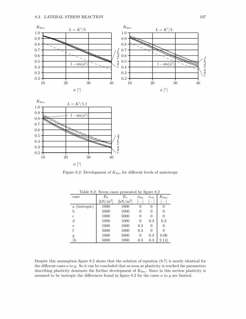
8.3. LATERAL STRESS REACTION 107
10 20 30 40
φ [◦]
0.2
0.3
0.4
0.5
0.6
0.7
0.8
0.9
1.0
K0ncL = K ′/5
1 - sin(φ′)
fbdeagc
............................................................................
....................................
.............................................................................................................................................................................................................................................................................................................................................................................................................................................................................
...........................................................................................................................................................................................................................................................................................................................................................................................................................................................................
.............................................................................................................................................................................................................................................................................................................................................................................................................................................................................
..........................
..........................
..........................
..........................
..........................
..........................
..........................
.......................... ............. ............. .........
10 20 30 40
φ [◦]
0.2
0.3
0.4
0.5
0.6
0.7
0.8
0.9
1.0
K0ncL = K ′/2
1 - sin(φ′)
fbdeagc
.....................................
...............................................................
..................................................................................................................................................................................................................................................................................................................................................................................................................................................................................
..............................................................................................................................................................................................................................................................................................................................................................................................................................................................................
...................................................................................................................................................................................................................................................................................................................................................................................................................................................................................
.............................................................................................................................................................................................................................................................................................................................................................................................................................................................................
................................................................................................................................................................................................................................................................................................................................................................................................................................................................................
.............................................................................................................................................................................................................................................................................................................................................................................................................................................................................
.................................................................................................................................................................................................................................................................................................................................................................................................................................................................................
..........................
..........................
..........................
..........................
..........................
..........................
..........................
.......................... ............. ............. .........
10 20 30 40
φ [◦]
0.2
0.3
0.4
0.5
0.6
0.7
0.8
0.9
1.0
K0ncL = K ′/1.1
1 - sin(φ′)
dfbeagc
.......................................................
.......................................
......................................................................................................................................................................................................................................................................................................................................................................................................................................................................................
....................................................................................................................................................................................................................................................................................................................................................................................................................................................................................
....................................................................................................................................................................................................................................................................................................................................................................................................................................................................................
............................................................................................................................................................................................................................................................................................................................................................................................................................................................................
......................................................................................................................................................................................................................................................................................................................................................................................................................................................................................
....................................................................................................................................................................................................................................................................................................................................................................................................................................................................................
...................................................................................................................................................................................................................................................................................................................................................................................................................................................................................
................................................................................................................................................................................
...................
..........................
..........................
..........................
..........................
..........................
..........................
..........................
..........................
............. ............. .........
Figure 8.2: Development of K0nc for different levels of anisotropy
Table 8.2: Seven cases presented by figure 8.2case Eh Ev νhh νvh K0nc
[kN/m2] [kN/m2] [ - ] [ - ] [ - ]a (isotropic) 1000 1000 0 0 0b 5000 1000 0 0 0c 1000 5000 0 0 0d 1000 1000 0 0.3 0.3e 1000 1000 0.3 0 0f 5000 1000 0.3 0 0g 1000 5000 0 0.3 0.06(h 5000 1000 0.3 0.3 2.14)
Despite this assumption figure 8.2 shows that the solution of equation (8.7) is nearly identical forthe different cases a to g. So it can be concluded that as soon as plasticity is reached the parametersdescribing plasticity dominate the further development of K0nc. Since in this section plasticity isassumed to be isotropic the differences found in figure 8.2 for the cases a to g are limited.

108 CHAPTER 8. PRACTICAL APPLICATIONS
8.4 Consolidation around a vertical drain
............................................................................................................................................................................................................................................................................................................................
.....
.....
.....
.....
.....
.....
.....
.....
.....
.....
.....
.....
.....
.....
.....
.....
.....
.....
.....
.....
.....
.....
.....
.....
.....
.....
.....
.....
.....
.....
.....
.....
.....
.....
.....
.....
.....
.....
.....
.....
.....
.....
.....
.....
.....
.....
.....
.....
.....
.....
.....
.....
.....
.....
.....
.....
.....
.....
.....
.....
.....
.....
.....
.....
.....
.....
.....
.....
.....
.....
.....
.....
.....
.....
.....
.....
.....
.....
.....
.....
.....
.....
.....
.......................
...................
..............................................
..............................................
..............................................
.................
................................................................................
..................................................
.........................................................................................................................................................................................................................
...........................................
........................................................................................................................................................................................................................
............................................................
...........................
........................................................................................................................................................................................................................
.....
.....
.....
.
.....
.....
.....
.....
.....
.....
.....
.....
.....
.....
.....
.....
.....
.....
.....
.....
.....
.....
.....
.....
.....
.....
.....
.....
.....
.....
.....
.....
.....
.....
.....
.....
.....
.....
.....
.....
.....
.....
.....
.....
.....
.....
.....
.....
.....
.....
.....
.....
.....
.....
.....
.....
.....
.....
.....
.....
.....
.....
.....
.....
...
.....
.....
.....
.....
.....
.....
.....
.....
.....
.....
.....
.....
.....
.....
.....
.....
.....
.....
.....
.....
.....
.....
.....
.....
.....
.....
.....
.....
.....
.....
.....
.....
.....
.....
.....
.....
.....
.....
.....
.....
.....
.....
.....
.....
.....
.....
.....
.....
.....
.....
.....
.....
.....
.....
.....
.....
.....
.....
.....
.....
... .....................................
.....
.....
.....
.....
.....
.....
.....
.....
.....
.....
.....
.....
.....
.....
.....
.....
.....
.....
.....
.....
.....
.....
.....
.....
.....
.....
.....
.....
.....
.....
.....
.....
.....
.....
.....
.....
.....
.....
.....
.....
.....
.....
.....
.....
.....
.....
.....
.....
.....
.....
.....
.....
.....
.....
.....
.....
.....
.....
.....
.....
.....
.....
.....
.....
.....
..
z
rR
σb
σrh
ρθ
qrqr
..........................
............. ............. ............. ............. ............. ............. ............. .................................... ............. .............
............................................
.....
.....
...
.....
.....
...
.....
.....
...
.....
.....
...
.....
.....
...
.....
.....
...
.....
.....
...
.....
.....
...
.....
.....
...
.....
.....
...
.....
.....
...
...
.....
.....
...
.....
.....
...
.....
.....
...
.....
.....
...
.....
.....
...
.....
.....
...
.....
.....
...
.....
.....
...
.....
.....
...
.....
.....
...
.....
.....
...
.....
.....
...
...
...................................................................................................................................................................
...................................................................
..............................................................................
...............................................................................
.............. .......................................................................................................................
...................
........................................................................................................................
.....
.....
....
.....
.....
.....
....
......................................................................................................................
.....
.....
....
.....
.....
.....
....
................................................................................................................
.....
.....
....
...................
......................................................................................................
.....
.....
....
.....
.....
.....
....
..........................................................................................
.....
.....
....
.....
.....
.....
....
...............................................................................
.....
.....
....
.....
.....
.....
....
.....................................................................
.....
.....
....
.....
.....
.....
....
..............................................................
.....
.....
....
.....
..............
............................................................
.....
.....
....
.....
.....
.....
....
.......................................................................................
.......................................................................................
....................................................................
......................................................................................
....................
....................................................................
......................................................................................
....................
.......................................................................................
.......................................................................................
.......................................................................................
....................................................................
......................................................................................
....................
....................................................................
...........................................................................................................................................................................................................................................................................................................................................................
....................
....................................................................
......................................................................................
.................... .....
.....
.....
.....
.....
.....
.....
.....
.....
.....
.....
.....
.....
.....
.....
.....
.....
.....
.....
.....
.....
.....
.....
.....
.....
.....
.....
.....
.....
.....
.....
.....
.....
.....
.....
.....
.....
.....
.....
.....
.....
.....
.....
.....
.....
.....
.....
.....
.....
.....
.....
.....
.....
.....
.....
.....
.....
.....
.....
..
Figure 8.3: Problem definition for a verticaldrain
To visualise the influence of anisotropy on the con-solidation as observed in the field this section dis-cusses consolidation behaviour of anisotropic soilaround a vertical drain. Application of a differentset of boundary conditions to the axial symmet-ric consolidation problem described in chapter 5leads to the solution for the consolidation problemaround vertical drains. The boundary conditionsare sketched in figure 8.3, in which R representsthe radius of the cylinder which is influenced bythe drain. The parameter ρ represents the radiusof the drain and qr the expelled pore water flow.Equivalent to the solutions presented by chapter 5a redistribution of stresses will occur. The surfaceremains flat, ∂εzz/∂r = 0.
Solutions to the consolidation problem aroundvertical drains for isotropic soil are given by Bar-ron [10] and by De Leeuw [53]. Both solutions as-sume a flat surface. This is achieved in the Barronsolution by incorporating an average pore pressuredevelopment. The De Leeuw solution is based onthe Biot equations equivalent to the solution for the anisotropic case given in appendix G. Inengineering practice the Barron solution is often used in combination to the average degree ofconsolidation U in which U is defined by:
U =
∫ R
ρ
2πr
π (R2 − ρ2)
σwσb
dr (8.8)
Figure 8.4 shows a comparison between the Barron and the De Leeuw solution. Note that inthis section the sign convention according to section 2.1 is adopted. For the average developmentof consolidation, (1 - U) versus T , the Barron and the De Leeuw solution predict an equivalentconsolidation process. However at individual values for r and t differences occur. This is shownfigure 8.4b. For the initial pore pressure reaction the Barron solution predicts a parabolic distrib-ution of excess pore pressure in r direction. While for t = 0+ on average σw/σb = 1, for r = R theBarron solution predicts σw/σb = 1.17. In contrast the De Leeuw solution predicts σw/σb = 1 atall r except for r = ρ due to the boundary condition of no excess pore pressure inside the drain,σw/σb = 0 at r = ρ.
Appendix G gives the extension of the De Leeuw solution to anisotropic conditions. Figure 8.5shows the calculated pore pressure development found at r = R for the seven cases presented bytable 5.1, which is repeated by table 8.3. It should be noted that case a corresponds to the DeLeeuw solution. As shown by De Leeuw [53] the isotropic solution does not show the Mandel-Cryereffect for realistic boundary conditions. Chapter 5 shows that presence of the Mandel–Cryer effectin the mathematical solution is explained by the integration coefficient f(t). For ∂f(t)/∂t = 0 theanalytical solutions will not show a Mandel–Cryer effect. De Leeuw [53] gives for f(t):
f(t) = −4Grρ
R2 − ρ2
(f1ρ
− f2R
)− f3 − 2f4
In which f1 represents radial displacements at r = R, f2 radial displacements at r = ρ, f3 the loadapplied on top, f3 = σb and f4 the water pressure in the drain.
Assuming enough drainage capacity f4 remains zero during consolidation. In engineering prac-tice the radial deformation at r = ρ and r = R can be disregarded. The function f(t) reduces

8.4. CONSOLIDATION AROUND A VERTICAL DRAIN 109
10−5 10−4 10−3 10−2 0.1 1 10 100
T =ct
R2
0.0
0.2
0.4
0.6
0.8
1.0
1 − U
.........................................................................................................................................................
....................................
..............................................................................................................................................................................................................................................................................................................................................................................................................................................................................
............. ............. ............. ............. ............. ............. ............. ..........................
.............
.............
.............
.............
.............
.............
.....
.....
...
.....
.....
...
.....
.....
...
.....
.....
...
.....
.....
...
.....
.....
...
.............
.......................... ............. ..........
0.0 0.2 0.4 0.6 0.8 1.0
r/R
0.0
0.2
0.4
0.6
0.8
1.0
1.2σw/σb
t = 0+
r = ρ
...................................
.....
.....
.....
.....
.....
.....
.....
.....
.....
.....
.....
.....
.....
.....
.....
.....
.....
.....
.....
.....
.....
.....
.....
.....
.....
.....
.....
.....
.....
.....
.....
.....
.....
.....
.....
.....
.....
.....
.....
.....
.....
.....
.....
.....
.....
.....
.....
.....
.....
.....
.....
.....
.....
.....
.....
.....
.....................................................................................................................................................................................................................................................................................................
........................................................................
.....
........
.............
.............
.....
.....
...
.............
.............
.............
.............
.............
..........................
.............
.............
.............
.............
.............
..........................
............. .............
............. ............. .............
De Leeuw solutionBarron solution
Figure 8.4: a) Development of U b) Initial pore pressure reaction
to -σb. After application the load remains constant and therefore f(t) reduces to a constant. Foranisotropic conditions f(t) is expressed by equation (G.60). Equation (G.60) is a function of timeeven for constant boundary conditions.
Table 8.3: Seven cases for visualisation of the solutions of appendices Gcase Eh Ev νhh νvh A+ 2Ghh
[kN/m2] [kN/m2] [ - ] [ - ] [ kPa ]a (isotropic) 1000 1000 0 0 1000b 5000 1000 0 0 5000c 1000 5000 0 0 1000d 1000 1000 0 0.3 1110e 1000 1000 0.3 0 1099f 5000 1000 0.3 0 5494.5g 1000 5000 0 0.3 1019
Figure 8.5 clearly shows the influence of anisotropy. This influence extends beyond the influenceof the coefficient of consolidation c. If the influence of anisotropy was limited to that of thecoefficient of consolidation alone, the curves presented by figure 8.5 would be identical. For cases band f a small Mandel–Cryer effect is found at r = R. These cases have the longest hydrodynamicperiod. Cases a, d and e represent the isotropic case respectively deviations in νhh and νvh. Theinfluence of νhh and νvh appears to be small. Cases c and g show a rapid decay in excess porepressure. The solution for case b converges badly for small values of t. This is shown by figure 8.5by an initial σw/σb < 1 for case b.
Application of equation (8.8) to the anisotropic solution leads to the expression for the averagedegree of consolidation U for anisotropic conditions. Figure 8.6 shows the results. In the develop-ment of U the Mandel–Cryer effect is no longer visible. However the influence on the hydrodynamicperiod is still clearly shown. The cases c and g show a short hydrodynamic period while for b andf a relatively long period is found. Again case b converges badly for small values of t, shown infigure 8.6 by an initial (1 - U) > 0.
The coefficient of consolidation is given by c = (A+ 2Ghh)k/γw. The parameters k and γw arekept constant for each of the seven cases presented by table 8.3. Cases b and f have the largest
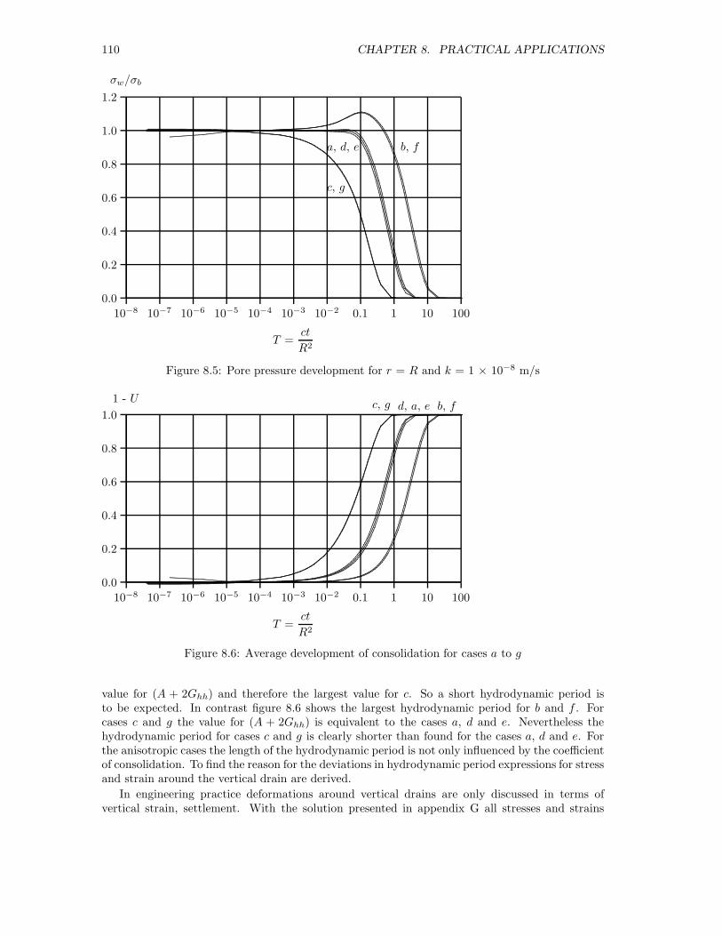
110 CHAPTER 8. PRACTICAL APPLICATIONS
10−8 10−7 10−6 10−5 10−4 10−3 10−2 0.1 1 10 100
T =ct
R2
0.0
0.2
0.4
0.6
0.8
1.0
1.2
σw/σb
...........................................................................................................................................................................................................................................................................................................................................................................................................................................................................................................................................................................................................................................................................................................................................................................................................................................................................................................................
..........................................................................................................
..........................................................................................................................................................................................
.........................................................
................................................................
..............................................................................................................................................................................................................................................................................................................................................................................................................................................................................................................................
................................................................................................................................................................................................................................................................................................................................................................................................................................................................................................................................................................................................................................................................................................................................................................................................................................................................................
........................................................................................................................................................................................................................................................................................................................................................................................................................................................................................................................................................................................................................................................................................................................................................................................................................................................................................................................
................................................................................................................................................................................................................................................................................................................................................................................................................................................................................................................................................................................................................................................................................................................................................................................................................................................................................................................................
...............................................................................................................................................................................................................................................................................................................................
.......................................
....................................................................................................................................................................................................................................................................................................................................................................................................................................................................................................................................................................................
.................................................................................................................................................................................................................................................................................................................................................................................................................................................................................................................................................................................................................................................................................................................................................................................................................................................................................
b, fa, d, e
c, g
Figure 8.5: Pore pressure development for r = R and k = 1 × 10⁻⁸ m/s
10−8 10−7 10−6 10−5 10−4 10−3 10−2 0.1 1 10 100
T =ct
R2
0.0
0.2
0.4
0.6
0.8
1.0
1 - U
..............................................................................................................................................................................................................................................................................................................................................................................
.....................................
..................................................................................................................................................................................................................................................................................................................................................................................................................................................................................................................................
.........................................................................................................................................................................................................................................................................................................................................................................................................
......................................................................................................................................................................................................................................................................................................................................................................................................................................................
.........................................
........................................................................................................................................................................................................................................................
...........................................................
..............................
...........................................................................................................................................................................................................................................................................................................................................................................................................................................................................................................................................................................
.......................................................................................................................................................................................................................................................................................................................................
.......................................................
.............................................................................................................................................................................................................................................................................................................................................................................................................................................................................................................................................
..............................................................................................................................................................................................................................................................................................................................................................
...............................................
.................................................................................................................................................................................................................................................................................................................................................................................................................................................................................................................................
..........................................................................................................................................................................................................................................................................................................................................................................................................
..................................................................................................................................................................................................................................................................................................................................................................................................................................................................................................
...............................................................................................................................................................................................................................................................................
...............................................
.............................................................................................................................................................................................................................................................................................................................................................................................................................................................................................................................................................................................
c, g d, a, e b, f
Figure 8.6: Average development of consolidation for cases a to g
value for (A + 2Ghh) and therefore the largest value for c. So a short hydrodynamic period isto be expected. In contrast figure 8.6 shows the largest hydrodynamic period for b and f . Forcases c and g the value for (A + 2Ghh) is equivalent to the cases a, d and e. Nevertheless thehydrodynamic period for cases c and g is clearly shorter than found for the cases a, d and e. Forthe anisotropic cases the length of the hydrodynamic period is not only influenced by the coefficientof consolidation. To find the reason for the deviations in hydrodynamic period expressions for stressand strain around the vertical drain are derived.
In engineering practice deformations around vertical drains are only discussed in terms ofvertical strain, settlement. With the solution presented in appendix G all stresses and strains

8.4. CONSOLIDATION AROUND A VERTICAL DRAIN 111
around a vertical drain can be derived. For two typical cases, f and g radial effective stress σ′r,
radial strain εr, radial displacement ur, and volumetric strain e, are shown by figure 8.7. It shouldbe noted that the tangential strain εθ, is related to the radial displacement by εθ = ur/r.
Figure 8.7 shows that radial deformations and radial strain are concentrated around the verticaldrain. Initially the radial stress at r = ρ equals the loading applied at the top while σ′
r remainsunaltered at other locations along the radius. When consolidation progresses σ′
r first increases forsmall values for r and decreases for larger values for r. When consolidation progresses further σ′
r
reduces to K0 × σb with K0 given by equation (8.1). For case νvh = 0 and therefore K0 and σ′r
reduce to 0. For case g K0 = 0.06 and σ′r/σb reduces to 0.06.
Due to the concentration of radial effective stress around the drain, radial strain is also concen-trated around the drain as shown by the second part of figure 8.7. Development of εr is equivalentto σ′
r. Initially only at r = ρ radial strain develops. As consolidation proceeds εr/σb is positivefor small values for r and negative for R. For loading conditions σb is negative. So positive valuefor εr/σb gives a negative εr. This means that at early stages of the consolidation process the soilcontracts around the drain and expands at the outer radius.
The third part of figure 8.7 shows the displacements to be expected around a vertical drain.According to the boundary conditions ur = 0 at r = ρ and r = R. The largest radial displace-ments are found at short distance of the drain. Initially after loading the radial displacementsare negligible when consolidation progresses ur increases first and decrease later until no radialdisplacements remain. The location of the maximum peak value moves from small values for r tolarge values for R. The location of the maximum radial displacement corresponds to the locationat which εr changes sign.
The most remarkable difference between cases f and g is found in the development of volumetricstrain. For case f is initially found e = 0 except at r = ρ. Only at r = ρ the soil behaves initiallydrained and volumetric changes occur while the remaining soil behaves undrained and does notshow any change in volume. When time progresses the volumetric strain progresses from the innercore to the outer radius until the final deformation is reached. For case g, at r = ρ, the initialvolumetric strain exceeds its final value. When consolidation progresses the peak value reduceshowever the area for which the volumetric strain exceeds its final value increases. During a furtherdevelopment of consolidation volumetric strain develops to its final value leading to an expansionof the soil around the drain for case g. At the outer radius the soil still contracts. This expansionof the soil around the drain explains the relatively short consolidation period shown by figure 8.6.
It is therefore concluded that anisotropy in soft soil influences the consolidation behaviourof soft soil around a vertical drain. Depending on the ratio of horizontal to vertical stiffnessthe hydrodynamic period is longer or shorter than found for isotropic soil types. The differencein hydrodynamic period between isotropic and anisotropic soil is larger than expected from thedifference in coefficient of consolidation alone, as shown by figure 8.6. If the influence of anisotropyon the consolidation behaviour did depend only on the coefficient of consolidation all graphs infigure 8.6 would be equivalent.
Anisotropy of soft soil influences the consolidation behaviour by development of the radialstress and strain that occurs around the drain. Soil tends to contract around the drain. Thiscontraction is strongly influenced by the stiffness parameters. For Eh/Ev < 1 the contraction ofsoil around the drain is so strong that it overshoots the final volumetric strain. In a later phaseof the consolidation process, for Eh/Ev < 1 the soil even expands around the drain leading to theconsiderable acceleration of pore pressure dissipation given by figure 8.6 for cases c and g.
The assumption of uniform vertical strain, ∂εzz/∂r = 0, during consolidation is an importantassumption. Without this assumption no redistribution of stress takes place and the phenomenadiscussed in this section will not be present. Measurements of a Mandel–Cryer peak inside a fieldof vertical drains are not known to the author. Deviations in hydrodynamic period are often foundin practice. However, a large number of explanations can be found for the individual cases in whicha possible redistribution of stresses in combination to anisotropy cannot be isolated.
If redistribution of stresses occurs in a field of drains and if it influences the consolidation

112 CHAPTER 8. PRACTICAL APPLICATIONS
0.0 0.2 0.4 0.6 0.8 1.0
r/R
−0.2
0.0
0.2
0.4
0.6
0.8
1.0
σ′r/σb [ - ]
case f.....................................................................................................................................................................................................................................................................................................................................................................................................................................................................................................................................................................................................................
......................................................................................
.......................... .......................... ...........
..........................
..........................
..........................
..........................
..........................
.................................................... .......................... .......................... .......................... .......................... .......................... .......................... .......................... ...
..........................
..........................
..........................
....................................................
....................................................
.......................... .......................... .......................... .......................... .......................... .......................... .........
..........................
..........................
..........................
....................................................
....................................................
.......................... .......................... .......................... .......................... .......................... .......................... ...
..........................
..........................
....................................................
.................................................... .......................... .......................... .......................... .......................... .......................... .......................... .....
..........................
....................................................
.................................................... .......................... .......................... .......................... .......................... .......................... .......................... ...........
...... ...... ...... ...... ......
...... ...... ...... ...... ...... ...... ...... ...... ...... ...... ...... ...... ...... ...... ...... ...... ...... ...... ...... ...... ...... ......
t = 0
intermediate t
t = 400 000 s
0.0 0.2 0.4 0.6 0.8 1.0
r/R
−0.2
0.0
0.2
0.4
0.6
0.8
1.0
σ′r/σb [ - ]
case g.........................................................................................................................................................................................................................................................................................................................................................................................................................................................................................................................................................................................................................
..........................
..........................
..........................
..........................
..........................
.................................................... ..........................
.......................... .......................... .......................... .......................... .......................... .......................... ....................
..........................
..........................
....................................................
.................................................... .......................... .......................... .......................... .......................... .......................... .......................... .........................
..........................
..........................
....................................................
.................................................... .......................... .......................... .......................... .......................... .......................... ..........................
.................................................... .......................... .......................... .......................... .......................... .......................... .......................... .......................... .......................... ........
.......................... .......................... .......................... .......................... .......................... .......................... .......................... .......................... .......................... ................................ ...... ...... ...... ...... ...... ...... ...... ...... ...... ...... ...... ...... ...... ...... ...... ...... ...... ...... ...... ...... ....
0.0 0.2 0.4 0.6 0.8 1.0
r/R
−0.2
0.0
0.2
0.4
0.6
0.8
1.0
εr/σb × 10−3 [ - ]
.................................................................................................................................................................................................................................................................................................................................................................................................................................
.................................................... .......................... .......................... .......................... .......................... .......................... .......................... .......................... .......................... ..........
.................................................... .......................... .......................... .......................... .......................... .......................... .......................... .......................... .......................... ......
.................................................... .......................... .......................... .......................... .......................... .......................... .......................... .......................... .......................... .....
.......................... .......................... .......................... .......................... .......................... .......................... .......................... .......................... .......................... .......................... ..
.......................... .......................... .......................... .......................... .......................... .......................... .......................... .......................... .......................... ..........................
...... ...... ...... ...... ...... ...... ...... ...... ...... ...... ...... ...... ...... ...... ...... ...... ...... ...... ...... ...... ...... ....
0.0 0.2 0.4 0.6 0.8 1.0
r/R
−0.2
0.0
0.2
0.4
0.6
0.8
1.0
εr/σb × 10−3 [ - ]
.........................................................................................................................................................................................................................................................................................
............................................................................................................................................................................................................................................................................................................................
..........................
..........................
..........................
..........................
..........................
.................................................... ..........................
.......................... .......................... .......................... .......................... .......................... .......................... ................
..........................
..........................
....................................................
.................................................... .......................... .......................... .......................... .......................... .......................... .......................... .......................
..........................
..........................
....................................................
.......................... .......................... .......................... .......................... .......................... .......................... .......................... ..........................
.................................................... .......................... .......................... .......................... .......................... .......................... .......................... .......................... .......................... ........
.......................... .......................... .......................... .......................... .......................... .......................... .......................... .......................... .......................... ................................ ...... ...... ...... ...... ...... ...... ...... ...... ...... ...... ...... ...... ...... ...... ...... ...... ...... ...... ...... ...... ....
0.0 0.2 0.4 0.6 0.8 1.0
r/R
0
1
2
3
4
5
ur/(σb ×R) × 10−5
[m2/kN]
..........................................................................................................................................................................................................................................................................................................................................................................................................................
.......................... .......................... .......................... .......................... .......................... .......................... .......................... .......................... .......................... ................
..............................................
.......................... .......................... .......................... .......................... .......................... .......................... .......................... .......................... ........................
..............................................
.......................... .......................... .......................... .......................... .......................... .......................... .......................... .......................... ........................
....................
..........................
.................................................... .......................... .......................... .......................... .......................... .......................... .......................... ..................
..................
.......................... .......................... .......................... .......................... .......................... .......................... .......................... .......................... .......................... .......... ...... ...... ...... ...... ...... ...... ...... ...... ...... ...... ...... ...... ...... ...... ...... ...... ...... ...... ...... ...... .....
0.0 0.2 0.4 0.6 0.8 1.0
r/R
0
1
2
3
4
5
ur/(σb ×R) × 10−5
[m2/kN]
......................................................................................................................................................................................................................................................................................................................................................................................................
.....
.....
.....
.....
.
.....
.....
.....
.....
.....
.
..........................
....................................................
.................................................... .......................... .......................... .......................... .......................... .......................... ....................
.....
.....
.....
.....
.
.....
.....
.....
.....
.....
.
.....
.....................
..........................
..........................
....................................................
....................................................
....................................................
....................................................
....................................
.....
.....
.....
.....
.
.....
.....
.....
...........
..........................
....................................................
.......................... ....................................................
....................................................
....................................................
....................................................
......................................................
..........................
.......................... .......................... .......................... .......................... .......................... ..........................
...............................................................
............... .........................
. .......................... .......................... .......................... .......................... .......................... .......................... .......................... .......................... ....... ...... ...... ...... ...... ...... ...... ...... ...... ...... ...... ...... ...... ...... ...... ...... ...... ...... ...... ...... ...... ....
0.0 0.2 0.4 0.6 0.8 1.0
r/R
−0.2
0.0
0.2
0.4
0.6
0.8
1.0
e/σb × 10−3 [ - ]
.................................................................................................................................................................................................................................................................................................................................................................................................................................
.................................................... .......................... .......................... .......................... .......................... .......................... .......................... .......................... .......................... .....
.......................... .......................... .......................... .......................... .......................... .......................... .......................... .......................... .......................... .......................... ..
.......................... .......................... .......................... .......................... .......................... .......................... .......................... .......................... .......................... .......................... .
.......................... .......................... .......................... .......................... .......................... .......................... .......................... .......................... .......................... ..........................
.......................... .......................... .......................... .......................... .......................... .......................... .......................... .......................... .......................... ..........................
...... ...... ...... ...... ...... ...... ...... ...... ...... ...... ...... ...... ...... ...... ...... ...... ...... ...... ...... ...... ...... ....
0.0 0.2 0.4 0.6 0.8 1.0
r/R
−0.2
0.0
0.2
0.4
0.6
0.8
1.0
e/σb × 10−3 [ - ]
....................................................................................................................................................................................................................................................................................................................................................................................................................................................................................................................................................................................................................
..........................
..........................
..........................
..........................
..........................
.......................... .......................... .......................... .......................... .......................... .......................... .......................... .......................... ..........................
..........................
....................................................
....................................................
.......................... .......................... .......................... .......................... .......................... .......................... ..........................
....................................................
....................................................
.................................................... .......................... .......................... .......................... .......................... .......................... ..........
.......................... .......................... .......................... .......................... .......................... .......................... .......................... .......................... .......................... .......................... ...
.......................... .......................... .......................... .......................... .......................... .......................... .......................... .......................... .......................... ..........................
...... ...... ...... ...... ...... ...... ...... ...... ...... ...... ...... ...... ...... ...... ...... ...... ...... ...... ...... ...... ...... ....
Figure 8.7: Radial effective stress and strain for cases f and g at t = 0, 500, 5 000, 10 000, 50 000,100 000 and 400 000 s

8.4. CONSOLIDATION AROUND A VERTICAL DRAIN 113
development can only be established for special conditioned cases. An example of these specialconditioned cases is a model test. Several model studies on the topic of consolidation aroundvertical drains are available.
0.01 0.1 1 10 102 103
t [s]
0.0
0.2
0.4
0.6
0.8
1.0
1.2σw/σw0
...........................................................................................................................................................
........................................................................................................................................................................................................................................................................................................................................................................................................................................................................................................................................................................................................................................................................................................................................................................................................................................................................................................................................................................
............. ............. ............. ............. ..........................
..........................
.....................................................................................................................
.......................... ..............................................................................
reference area
floating piles
Figure 8.8: Measured pore pressure develop-ment in centrifuge test
Zwanenburg, Van & Brassinga [84] describea centrifuge test in which consolidation aroundsand piles and sand walls is studied. In pro-totype measures the test set–up consists of 9 mthick clay layer, a 0.45 m thick sand layer on topand a 0.90 m thick sand layer underneath. Thesand piles and walls are placed floating, with0.90 m clay between sand pile or wall and lowersand layer, or non–floating when the sand pileor wall is placed on the lower sand layer. Theclay consists of speswhite clay with a water con-tent W = 0.57 - 0.58 and unit weight γ = 16.3kN/m2. The load is applied in three steps toa maximum of 100 kPa. For each configurationtwo pore pressure transducers are placed, one at2.7 m below top side of the clay layer and one at5.4 m. These locations correspond to 1/3 and2/3 of the floating pile length. The transduc-ers are placed at the middle between two sandpiles or walls. Besides the pore pressure devel-opment settlement is measured at the originalsurface level at the middle between the piles orwalls and at the top of the sand pile or wall.
The different configurations are tested in one test set–up. The available drainage field is sep-arated in eight sections. Two sections involve sand walls, five sections involve sand piles. In onesection no piles or walls are applied. This section is referred to as reference section. Measurementsare conducted at the sand pile or wall located in the centre of the section. For the reference sectionmeasurements are conducted at the middle of the section.
The level of anisotropy of the speswhite clay is expected to be negligible. Therefore, accordingto the De Leeuw solution, no Mandel–Cryer peak is to be expected between the sand piles. Thiscorresponds to figure 8.8, which shows a monotonic decay in pore pressure development in the clayin the floating drain section. In this section no Mandel–Cryer peak is found.
The reference section is connected at three sides to sections including sand piles. The horizontaldistance between the pore pressure transducer in the reference section and the surrounding rowof drains is of the same order in magnitude as the vertical distance to the upper and lower sandlayer. It can therefore be concluded that pore water flow during consolidation will not be purelyvertically.
Figure 8.8 shows the pore pressure development after the third loading phase. Despite theabsence of a stiff plate on top the measurements show clearly a Mandel–Cryer peak. It cantherefore be concluded that a stiff plate on top is not necessary for a redistribution of stresses. Analternative cause for a redistribution of stresses is internal friction. Friction is not considered in theanalytical solutions presented by chapter 5. To which extend internal friction can be consideredas a source for redistribution of stresses forms a topic a further study. So, depending on the actualgeometry, influence of anisotropy in stiffness of soil that consolidates around a vertical drain is tobe expected.

114 CHAPTER 8. PRACTICAL APPLICATIONS

Appendix A
Compression of a solid sphere
In this appendix the volume loss of solid spheres due to indentation is studied. The results of thisanalysis are used in section 2.3.2 to determine the corresponding compressibility of solid particles.A mathematical analysis of dented spheres is presented by Timoshenko & Goodier [72].
.............................................................................................................................................................................................................................................................................
..................................
..........................
................................................
.....
..................
..................
........................................................................................................................................................................................................................................................................................................................................................................................................................................................
.............
..............................................................................................................................................................................................................................................................
......................................................................................................................................
.............
....................................................................................................................................................................................................................................................................................................................................................................................
.................
. . ....... .
...... . .
z
x
y
R
a
√R2 − a2
φ
θ
ρ
........
........
........
........
........
........
........
........
........
........
........
........
........
........
........
........
........
........
........
........
........
........
........
........
..................
Figure A.1: Compression of a sphere, definition of parameters
Soil particles are simplified as perfect spheres. In a skeleton of spheres a specific sphere hasa limited number of contact points where it touches its adjacent spheres. If the spheres arecompressible they will be indented around these contact points. These indentations cause a volumeloss. In figure A.1 a part of a sphere is drawn. In the centre point of the sphere the x, y and zco-ordinate system and the system in spherical co-ordinates, θ, φ and ρ are given. The shadedarea is compressed due to the contact with a sphere below. The lower sphere does not need to beof equal size, however it still is a perfect sphere. The area of contact is a circle with a radius a.In this appendix first an expression for the radius of the dented area, a, is derived, followed by anexpression for the volume of the dented area. In deriving this solution linear elastic behaviour isassumed and a is assumed to be small in comparison to radii of the individual spheres.
Consider two spheres in contact, figure A.2, the lower sphere with radius R1 and the upper
115

116 APPENDIX A. COMPRESSION OF A SOLID SPHERE
sphere with radius R2. If no pressure is applied there is contact in only one single point. In thiscontact point a plane O tangent to both spheres can be drawn. On a distance r a point M islocated at the boundary of the lower sphere and a point N at the upper sphere. The distance fromplane O to M is indicated by z1 and to N by z2. With x1 = R1 − z1 an expression for z1 can befound:
R1 =√r21 + x2 = z1 + r1
with:
z21 ≪ 1, x1 ≃ R1
follows:
z1 =r2
2R1
Equivalent for z2:
z2 =r2
2R2
The total distance between M and N becomes:
z1 + z2 =r2
2R1+
r2
2R2=r2 (R1 +R2)
2R1R2
Compression in the direction normal to O by a force P creates a surface of contact. Whenholding plane O immovable the centre points of the spheres will approach each other by an amountα. The displacements w1 and w2 are caused by local deformation of the original contact point.The distance between M and N diminish by α− (w1 + w2). The points M and N are entering thecontact surface when:
α− (w1 + w2) = z1 + z2 = βr2, β =R1 +R2
2R2R2(A.1)
.............................
.........................................
.................................................................................................................................................................................................................
..............................................................................................................................................................................................
...............................................................................
.....
.....
.....
.....
.....
.....
.....
.....
.....
.....
.....
.....
.....
.....
.....
.....
.....
.....
.....
.....
.....
.....
.....
.....
.....
.....
.....
.....
.....
.....
.....
.....
.....
.....
.....
.....
.....
.....
.....
.....
.....
.....
.....
.....
.....
.....
.....
.....
.....
.....
.....
.....
.....
.....
.....
.....
.....
.....
.....
.....
.....
.....
.....
.....
.....
.....
.....
.....
.....
.....
.....
.....
.....
.....
.....
.....
.....
.....
.....
.............
.........
........................................................................................................................................................................................
.................
........................................................................................................................................................................................
.............
.....
.....
.....
.....
.....
.....
.....
.....
.....
.....
.....
.....
.....
.....
.....
.....
.....
..............
.............
•
•N
M
R2
R1
Oz2z1
z1
z2
.....
.....
.....
.....
.....
.....
.....
.....
.....
.....
.....
.....
.....
.....
....
..................................
.................
...................................................................................................................................................
................................................................................................................................................................................................................................................................................
...................
............................
.....................................................................................................................................................................................................................................................................................................................................
.................
.....
.....
.............................
..........................................................................................................................................
........
.....
.....
.....
.....
.....
.....
.....
.....
.....
.....
.....
.....
.....
.....
.....
.....
.....
.....
.....
.....
.....
.....
.....
.....
.....
.
..............................................................................................................................
............................................................................................................................................................................................................................
.....
...........•
ra
O
m
n
M
θ
ψ
Figure A.2: Two spherical bodies in contact A) side view B) top view on contact area

117
When creating the area of contact, with q representing the contact pressure it is found:
w1 =1 − ν2
1
πE1
∫ ∫qdsdψ
with:
k1 =1 − ν2
1
πE1, k2 =
1 − ν22
πE2
it holds:
w1 + w2 = (k1 + k2)
∫ ∫qdsdψ = α− βr2 (A.2)
So the next step is to find a pressure distribution q that fulfils equation (A.2). It can be shown thata distribution of pressure q over the contact surface is represented by the ordinates of a hemisphereof radius a constructed on the surface of contact. If q0 represents the pressure at the centre of thecontact surface then
q0 = ka
In which k is a constant factor representing the scale of the problem. So if the pressure in thecentre, q0, increases, the contact surface increases with the same amount. In figure A.2 the topview of the contact surface is presented. The contact surface has a radius a and a centre pointO. The points m and n are arbitrary points on the boundary and M on the chord mn. Since thepressure distribution has the shape of a hemisphere, the pressure distribution on top of the chordmn has the shape of half a circle with radius R. The line from point O perpendicular to the linemn divides mn in two equal parts. The radius R can then be expressed by: R = a cos θ. Sinceq0/a is a scale factor representing the scale of the problem the pressure active upon the chord mnis given by: ∫
q0ds =q0aA
In which A represents the area between the chord mn and the upper boundary of the pressuredistribution. A is then given by:
A =1
2πR2 =
1
2π (a cos θ)2 =
1
2πa2
(1 − sin2 θ
)
From figure A.2 it is found that a sin θ = r sinψ:
A =1
2π(a2 − r2sin2ψ
)
Application in equation (A.2) gives:
(w1 + w2) = (k1 + k2)
∫q0aAdψ
(w1 + w2) = (k1 + k2)
π∫
0
q0a
1
2π(a2 − r2sin2ψ
)dψ
(w1 + w2) =πq02a
(k1 + k2)
π∫
0
(a2 − r2sin2ψ
)dψ
With sin2 ψ = 12 − 1
2 cos 2ψ it follows:
(w1 + w2) =πq02a
(k1 + k2)
[a2ψ − r2ψ
2+
1
2· 1
2sin 2ψ
]ψ=π
ψ=0
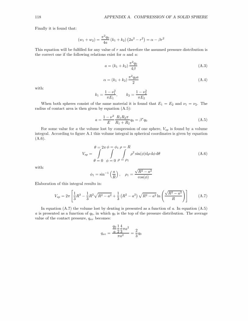
118 APPENDIX A. COMPRESSION OF A SOLID SPHERE
Finally it is found that:
(w1 + w2) =π2q04a
(k1 + k2)(2a2 − r2
)= α− βr2
This equation will be fulfilled for any value of r and therefore the assumed pressure distribution isthe correct one if the following relations exist for α and a:
a = (k1 + k2)π2q04β
(A.3)
α = (k1 + k2)π2q0a
2(A.4)
with:
k1 =1 − ν2
1
πE1, k2 =
1 − ν22
πE2
When both spheres consist of the same material it is found that E1 = E2 and ν1 = ν2. Theradius of contact area is then given by equation (A.5):
a =1 − ν2
E
R1R2π
R1 +R2q0 = β∗q0 (A.5)
For some value for a the volume lost by compression of one sphere, Vsp is found by a volumeintegral. According to figure A.1 this volume integral in spherical coordinates is given by equation(A.6).
Vsp =
θ = 2π∫
θ = 0
φ = φ1∫
φ = 0
ρ = R∫
ρ = ρ1
ρ2 sin(φ)dρ dφdθ (A.6)
with:
φ1 = sin−1( aR
), ρ1 =
√R2 − a2
cos(φ)
Elaboration of this integral results in:
Vsp = 2π
[1
3R3 − 1
3R2√R2 − a2 +
1
3
(R2 − a2
)√R2 − a2 ln
(√R2 − a2
R
)](A.7)
In equation (A.7) the volume lost by denting is presented as a function of a. In equation (A.5)a is presented as a function of q0, in which q0 is the top of the pressure distribution. The averagevalue of the contact pressure, qav becomes:
qav =
q0a
1
2
4
3πa2
πa2=
2
3q0

Appendix B
Lame constants for
cross–anisotropy
A familiar way to express stress in terms volumetric strain and distortional strain for an isotropiclinear elastic material is given by equation (B.1), see [72]:
σ′
ij = λeδij + 2µεij (B.1)
In which λ and µ are known as Lame constants:
λ = K +2
3G =
νE
(1 + ν) (1 − 2ν), µ = G =
E
2 (1 + ν)
In this appendix Lame - like constants are derived for cross–anisotropy. Equation 3.9, repeatedbelow, gives the full description of Hooke’s law for cross–anisotropic conditions.
εxx
εyy
εzz
γxy
γyz
γzx
=
1
Eh
−νhhEh
−νvhEv
0 0 0
−νhhEh
1
Eh
−νvhEv
0 0 0
−νvhEv
−νvhEv
1
Ev0 0 0
0 0 01
Ghh0 0
0 0 0 01
Gvh0
0 0 0 0 01
Gvh
σ′xx
σ′yy
σ′zz
τxy
τyz
τzx
(B.2)
119
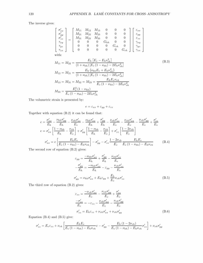
120 APPENDIX B. LAME CONSTANTS FOR CROSS–ANISOTROPY
The inverse gives:
σ′xx
σ′yy
σ′zz
τxyτyzτzx
=
M11 M12 M13 0 0 0M21 M22 M23 0 0 0M31 M23 M33 0 0 00 0 0 Ghh 0 00 0 0 0 Gvh 00 0 0 0 0 Gvh
εxxεyyεzzγxyγyzγzx
with:
M11 = M22 =Eh[Ev − Ehν
2vh
]
(1 + νhh) [Ev (1 − νhh) − 2Ehν2vh]
M12 = M21 =Eh(νhhEv + Ehν
2vh
)
(1 + νhh) [Ev (1 − νhh) − 2Ehν2vh]
M13 = M31 = M32 = M23 =EhEvνvh
Ev (1 − νhh) − 2Ehν2vh
M33 =E2v (1 − νhh)
Ev (1 − νhh) − 2Ehν2vh
(B.3)
The volumetric strain is presented by:
e = εxx + εyy + εzz
Together with equation (B.2) it can be found that:
e =σ′xx
Eh−νhhσ
′yy
Eh− νvhσ
′zz
Ev− νhhσ
′xx
Eh+σ′yy
Eh− νvhσ
′zz
Ev− νvhσ
′xx
Ev−νvhσ
′yy
Ev+σ′zz
Ev
e = σ′
xx
[1 − νhhEh
− νvhEv
]+ σ′
yy
[1 − νhhEh
− νvhEv
]+ σ′
zz
[1 − 2νvhEv
]
σ′
xx = e
[EhEv
Ev (1 − νhh) − Ehνvh
]− σ′
yy − σ′
zz
1 − 2νvhEv
EhEvEv (1 − νhh) − Ehνvh
(B.4)
The second row of equation (B.2) gives:
εyy =−νhhσ′
xx
Eh+σ′yy
Eh− νvhσ
′zz
Ev
−σ′yy
Eh=
−νhhσ′xx
Eh− εyy −
νvhσ′zz
Ev
σ′
yy = νhhσ′
xx + Ehεyy +EhEv
νvhσ′
zz (B.5)
The third row of equation (B.2) gives:
εzz =−νvhσ′
xx
Ev−νvhσ
′yy
Ev+σ′zz
Ev
−σ′zz
Ev= −εzz −
νvhσ′xx
Ev−νvhσ
′yy
Ev
σ′
zz = Ehεzz + νvhσ′
xx + νvhσ′
yy (B.6)
Equation (B.4) and (B.5) give:
σ′
zz = Evεzz + νvh
[EhEv
Ev (1 − νhh) − Ehνvhe− σ′
yy −Eh (1 − 2νvh)
Ev (1 − νhh) − Ehνvhσ′
zz
]+ νvhσ
′
yy

121
reformulating:
σ′
zz = Ce+Dεzz (B.7)
with:
C =νvhEhEv
Ev (1 − νhh) − 2Ehν2vh
D =E2v (1 − νhh) − EhEvνvhEv (1 − νhh) − 2Ehν2
vh
The first row of equation (B.2) gives:
εxx =σ′xx
Eh−νhhσ
′yy
Eh− νvhσ
′zz
Ev
σ′
xx = Ehεxx + νhhσ′
yy +EhEv
νvhσ′
zz (B.8)
Combination of equation (B.5) and (B.8) gives:
σ′
yy = νhh
[Ehεxx + νhhσ
′
yy +EhEv
νvhσ′
zz
]+ Ehεyy +
EhEv
νvhσ′
zz
σ′
yy
(1 − ν2
hh
)= νhhEhεxx + Ehεyy +
EhEv
νvhσ′
zz (1 + νhh)
with(1 − ν2
hh
)= (1 − νhh) (1 + νhh) :
σ′
yy =νhhEh1 − ν2
hh
εxx +Eh
1 − ν2hh
εyy +EhEv
νvh1 − νhh
σ′
zz (B.9)
Combination of (B.7) and (B.9) gives:
σ′
yy =νhhEh1 − ν2
hh
εxx +Eh
1 − ν2hh
εyy+
ν2vhE
2h
[Ev −
Ehνvh1 − νhh
]e
[Ev (1 − νhh) − Ehνvh] [Ev (1 − νhh) − 2Ehν2vh]
+νvhEhEv −
ν2vhE
2h
1 − νhhEv (1 − νhh) − 2Ehν2
vh
εzz
with:
εxx = e− εyy − εzz
σ′
yy =νhhEh1 − ν2
hh
e− νhhEh1 − ν2
hh
εyy +Eh
1 − ν2hh
εyy −νhhEh1 − ν2
hh
εzz +νvhEhEv −
ν2vhE
2h
1 − νhhEv (1 − νhh) − 2Ehν2
vh
εzz+
ν2vhE
2h
[Ev −
Ehνvh1 − νhh
]e
[Ev (1 − νhh) − Ehνvh] [Ev (1 − νhh) − 2Ehν2vh]
reformulation gives:
σ′
yy = Ae+ 2Ghhεyy +Bεzz (B.10)
122 APPENDIX B. LAME CONSTANTS FOR CROSS–ANISOTROPY
with:
A =νhhEh1 − ν2
hh
+
ν2vhE
2h
[Ev −
Ehνvh1 − νhh
]
[Ev (1 − νhh) − Ehνvh] [Ev (1 − νhh) − 2Ehν2vh]
=
=νhhEhEv + ν2
vhE2h
(1 + νhh) [Ev (1 − νhh) − 2Ehν2vh]
B =νvhEhEv −
ν2vhE
2h
1 − νhhEv (1 − νhh) − 2Ehν2
vh
− νhhEh1 − ν2
hh
=EhEv [νvh (1 + νhh) − νhh] − E2
hν2vh
(1 + νhh) [Ev (1 − νhh) − 2Ehν2vh]
Ghh =Eh
2 (1 + νhh)
The combination of equation (B.7), (B.8) and (B.10) gives:
σ′
xx = Ehεxx + νhhσ′
yy +EhEv
νvhσ′
zz
σ′
xx = Ehεxx + νhhAe+νhhEh1 + νhh
εyy + νhhBεzz +EhEv
νvh (Ce+Dεzz)
with: εyy = e− εxx − εzz
σ′
xx = Ehεxx + νhhAe+νhhEh1 + νhh
(e− εxx − εzz) + νhhBεzz +EhνvhEv
Ce+EhνvhEv
Dεzz
σ′
xx =
[νhhA+
νhhEh1 + νhh
+EhνvhEv
C
]e+
[Eh −
νhhEh1 + νhh
]εxx+
[νhhB +
EhνvhEv
D − νhhEh1 + νhh
]εzz
Reformulation of the individual terms gives:[νhhA+
νhhEh1 + νhh
+EhνvhEv
C
]=
ν2hhEh
1 − ν2hh
+νEh (1 − νhh)
(1 − νhh) (1 + νhh)+
νhhν2vhE
2h
(1 − νhh) [Ev (1 − νhh) − 2Ehν2vh]
+EhνvhEv
νvhEhEvEv (1 − νhh) − 2Ehν2
vh
=
νhhEh1 − ν2
hh
+νhhν
2vhE
2h − νhhν
2vhE
2h + ν2
vhE2h
(1 − νhh) [Ev (1 − νhh) − 2Ehν2vh]
=νhhEh1 − ν2
hh
+
ν2vhE
2h
(1 − νhh) [Ev (1 − νhh) − 2Ehν2vh]
=νhhEhEv + ν2
vhE2h
(1 + νhh) [Ev (1 − νhh) − 2Ehν2vh]
= A
Eh −νhhEh1 + νhh
=Eh (1 + νhh) − νhhEh
1 + νhh=
Eh1 + νhh
= 2Ghh
[νhhB +
EhνvhEv
D − νhhEh1 + νhh
]=νhhEhEv [νvh (1 + νhh) − νhh] − νhhν
2vhE
2h
(1 + νhh) [Ev (1 − νhh) − 2Ehν2vh]
+
EhνvhEv
E2v (1 − νhh) − EhEvνvhEv (1 − νhh) − 2Ehν2
vh
− νhhEh1 + νhh
=
EhEv [νvh (1 + νhh) − νhh] − ν2vhE
2h
(1 + νhh) [Ev (1 − νhh) − 2Ehν2vh]
= B
and is finally found:σ′
xx = Ae+ 2Ghhεxx +Bεzz (B.11)
123
The results can be summarised to:
σ′
xx = Ae+ 2Gεxx +Bεzz
σ′
yy = Ae+ 2Gεyy +Bεzz
σ′
zz = Ce+Dεzz
(B.12)
with:
A =νhhEhEv + ν2
vhE2h
(1 + νhh) [Ev (1 − νhh) − 2Ehν2vh]
B =EhEv [νvh (1 + νhh) − νhh] − ν2
vhE2h
(1 + νhh) [Ev (1 − νhh) − 2Ehν2vh]
C =νvhEhEv
Ev (1 − νhh) − 2Ehν2vh
D =E2v (1 − νhh) − EhEvνvhEv (1 − νhh) − 2Ehν2
vh
2Ghh =Eh
1 + νhh
After some elaboration it can be found that C = A + B:
A+B =νhhEhEv + ν2
vhE2h
(1 + νhh) [Ev (1 − νhh) − 2Ehν2vh]
+EhEv [νvh (1 + νhh) − νhh] − ν2
vhE2h
(1 + νhh) [Ev (1 − νhh) − 2Ehν2vh]
=
νhhEhEv + ν2vhE
2h + νvhEhEv + EhEvνhhνvh − νhhEhEv − ν2
vhE2h
(1 + νhh) [Ev (1 − νhh) − 2Ehν2vh]
=
νvhEhEv (1 + νhh)
(1 + νhh) [Ev (1 − νhh) − 2Ehν2vh]
= C
Adding shear stress and strain gives:
σ′
xx = Ae+ 2Ghhεxx +Bεzz
σ′
yy = Ae+ 2Ghhεyy +Bεzz
σ′
zz = (A+B) e+Dεzz
τxy = Ghhγxy
τyz = Gvhγyz
τzx = Gvhγzx
(B.13)
Note that for isotropic conditions, Eh = Ev = E, Ghh = Gvh = G and νhh = νvh = ν is found: A= νE/[(1 + ν)(1 − 2ν] = λ, B = 0 and D = 2Ghh = 2µ and equation (B.13) reduces to (B.1).Equation (B.13) gives a 5 parameter model which is in agreement with the requirements for across–anisotropic model according to section 3.1.

124 APPENDIX B. LAME CONSTANTS FOR CROSS–ANISOTROPY
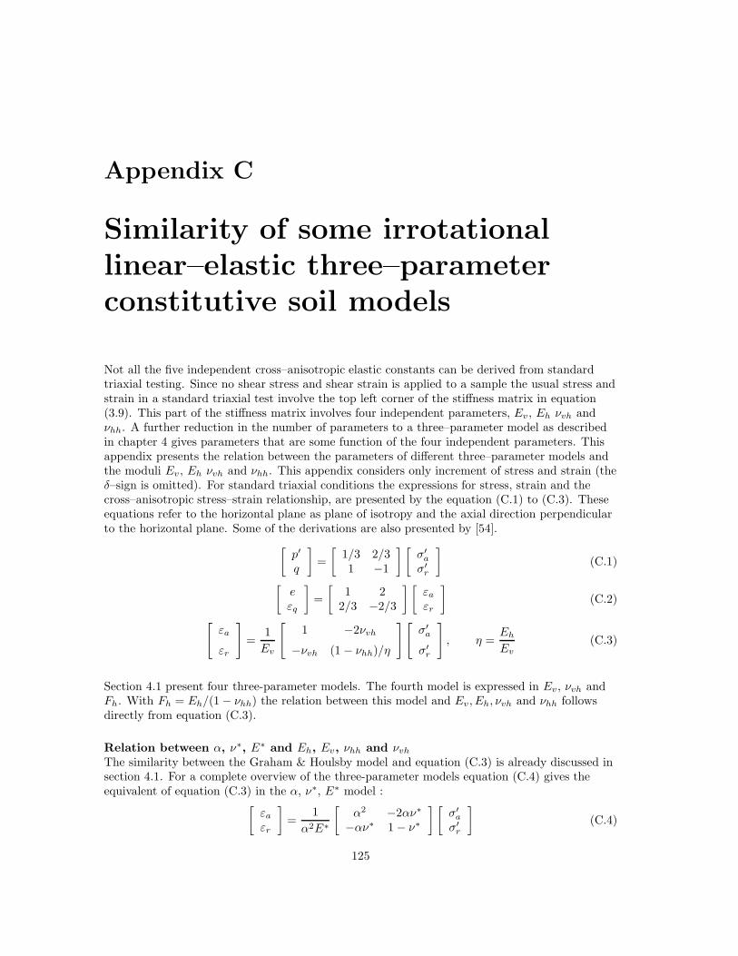
Appendix C
Similarity of some irrotational
linear–elastic three–parameter
constitutive soil models
Not all the five independent cross–anisotropic elastic constants can be derived from standardtriaxial testing. Since no shear stress and shear strain is applied to a sample the usual stress andstrain in a standard triaxial test involve the top left corner of the stiffness matrix in equation(3.9). This part of the stiffness matrix involves four independent parameters, Ev, Eh νvh andνhh. A further reduction in the number of parameters to a three–parameter model as describedin chapter 4 gives parameters that are some function of the four independent parameters. Thisappendix presents the relation between the parameters of different three–parameter models andthe moduli Ev, Eh νvh and νhh. This appendix considers only increment of stress and strain (theδ–sign is omitted). For standard triaxial conditions the expressions for stress, strain and thecross–anisotropic stress–strain relationship, are presented by the equation (C.1) to (C.3). Theseequations refer to the horizontal plane as plane of isotropy and the axial direction perpendicularto the horizontal plane. Some of the derivations are also presented by [54].
[p′
q
]=
[1/3 2/31 −1
] [σ′a
σ′r
](C.1)
[eεq
]=
[1 2
2/3 −2/3
] [εaεr
](C.2)
[εa
εr
]=
1
Ev
[1 −2νvh
−νvh (1 − νhh)/η
][σ′a
σ′r
], η =
EhEv
(C.3)
Section 4.1 present four three-parameter models. The fourth model is expressed in Ev, νvh andFh. With Fh = Eh/(1 − νhh) the relation between this model and Ev, Eh, νvh and νhh followsdirectly from equation (C.3).
Relation between α, ν∗, E∗ and Eh, Ev, νhh and νvhThe similarity between the Graham & Houlsby model and equation (C.3) is already discussed insection 4.1. For a complete overview of the three-parameter models equation (C.4) gives theequivalent of equation (C.3) in the α, ν∗, E∗ model :
[εaεr
]=
1
α2E∗
[α2 −2αν∗
−αν∗ 1 − ν∗
] [σ′a
σ′r
](C.4)
125

126 APPENDIX C. SIMILARITY OF THREE–PARAMETER MODELS
Comparison of both first terms of the matrices in equations (C.3) to (C.4) gives E∗ = Ev. Acomparison of the off-diagonal terms gives ν∗ = ανvh. Both expressions were already presented insection 4.1. A comparison of the last term of both matrices gives:
1 − ν∗
α2E∗=
1 − νhhEh
Implementing E∗ = Ev and ν∗ = ανvh renders this equation into:
(1 − νhh)EvEh
α2 + νvhα− 1 = 0
With α2 = Eh/Ev leads to α = νhh/νvh. This result is also presented in section 4.1 by equation(4.17).
Relation K∗, G∗, J and Ev, Eh, νhh and νvhIn the G∗, K∗, J model the stress–strain relationship is given by:
[p′
q
]=
[K∗ JJ 3G∗
] [eεq
](C.5)
An expression for G∗ can be found under the condition e = 0:
G∗ =1
3
(q
εq
)
e=0
With e = 0, it follows from equation (C.2) that εa = −2εr. Application to equation (C.3) gives:
σ′r
σ′a
= −1
2
(1 − 2νvh)Eh(1 − νhh)Ev − νvhEh
(C.6)
From equation (C.1):
q = σ′
a − σ′
r = σ′
a
(1 − σ′
r
σ′a
)
is found with equation (C.6) for q:
q =σ′a
2
[2 (1 − νhh)Ev + (1 − 4νvh)Eh
(1 − νhh)Ev − νvhEh
]
For e = 0 it is found from equation (C.2) that εq = εa = −2εr, with equation (C.3) and (C.6) isfound:
εq = σ′
a
[1
Ev+νvhEv
(1 − 2νvh)Eh(1 − νhh)Ev − νvhEh
]
For G∗ it is then found that:
G∗ =Ev6
[2 (1 − νhh)Ev + (1 − 4νvh)Eh
(1 − νhh)Ev − 2ν2vhEh
](C.7)
An expression for K∗ is found for the condition εq = 0:
K∗ =(pe
)
εq=0
127
For εq = 0 equation (C.2) gives εa = εr in combination with equation (C.3) is found:
σ′r
σ′a
=(1 + νvh)Eh
(1 − νhh)Ev + 2νvhEh(C.8)
From equation (C.1):
p′ =1
3σ′
a +2
3σ′
r = σ′
a
(1
3+
2
3
σ′r
σ′a
)
Combination with equation (C.8) yields:
p′ =σ′a
3
[(1 − νhh)Ev + 2 (1 + 2νvh)Eh
(1 − νhh)Ev + 2νvhEh
]
With εa = εr equation (C.2) and (C.3) yields:
e = 3σ′
a
[(1 − νhh)Ev − 2ν2
vhEhEv ((1 − νhh)Ev + 2νvhEh)
]
The expression for K∗ is given by:
K∗ =Ev9
[(1 − νhh)Ev + 2 (1 + 2νvh)Eh
(1 − νhh)Ev − 2ν2vhEh
](C.9)
An expression for J can be found for e = 0 or εq = 0. Here the option for e = 0 is elaborated:
J =
(p′
εq
)
e=0
Equation (C.2) indicates that for e = 0, εq = εa = −2εr. In combination to equation(C.3) and(C.6) it is found that:
εq = σ′
a
[1
Ev+νvhEv
(1 − 2νvh)Eh(1 − νhh)Ev − νvhEh
]=σ′a
Ev
(1 − νhh)Ev − 2ν2vhEh
(1 − νhh)Ev − νvhEh
From equation (C.1):
p′ =σ′a
3
(1 + 2
σ′r
σ′a
)
in combination with equation (C.6):
p′ =σ′a
3
[(1 − νhh)Ev − (1 − νvh)Eh
(1 − νhh)Ev − νvhEh
]
Finally, J is given by:
J =Ev3
[(1 − νhh)Ev − (1 − νvh)Eh
(1 − νhh)Ev − 2ν2vhEh
](C.10)
Relation between K ′, G′, J ′ and Ev, Eh, νvh and νhhIn the K ′, G′, J ′ model equation (C.3) is replaced by equation (C.11):
e
εq
=
1
K ′
1
J ′
1
J ′
1
3G′
p′
q
(C.11)

128 APPENDIX C. SIMILARITY OF THREE–PARAMETER MODELS
For p′ = 0 an expression for G′ can be found from equation (C.11):
G′ =1
3
(q
εq
)
p′=0
Equation (C.1) and the condition p′ = 0 gives σ′a = −2σ′
r. Application to the equations (C.2)and (C.3) gives:
εq =2
3(εa − εr) =
2
3
(1 + 2νvhEv
+1 − νhh
2Eh
)σ′
a
Since σ′a = −2σ′
r equation (C.1) yields σ′a = 2/3q and consequently εq becomes:
εq =4
9
(1 + 2νvhEv
+1 − νhh
2Eh
)q (C.12)
G′ is expressed by:
G′ =3
4
(1 + 2νvhEv
+1 − νhh
2Eh
) (C.13)
Equation (C.11) and q = 0 gives an expression for K ′
K ′ =
(p′
e
)
q=0
With q = 0 it follows from equation (C.1) that σ′r = σ′
a and further p′ = σ′a, in combination to
equations (C.2) and (C.3) gives:
e = εa + 2εr =
[1 − 4νvhEv
+2 (1 − νhh)
Eh
]p′
and for K ′:
K ′ =1
1 − 4νvhEv
+2 (1 − νhh)
Eh
(C.14)
The expression for J ′ can be found from the condition p′ = 0 or q = 0. Here, condition p′ = 0 isapplied:
J ′ =(qe
)
p′=0
From equation (C.1) it follows for p′ = 0 that σ′a = −2σ′
r, with combination of equations (C.2)and (C.3) it is found that:
e = εa + 2εr =1 − νvhEv
σ′
a −1 − νhhEh
σ′
a
Equation (C.1) with p′ = 0 and σ′a = 2/3q give for e:
e =2
3
(1 − νvh
Ev− 1 − νhh
Eh
)q
For J ′ it is found that:
J ′ =3
2
(1 − νvhEv
− 1 − νhhEh
) (C.15)
129
So far the axis of symmetry is assumed to be aligned in axial direction. If the axis of symmetry isaligned in radial direction equations (C.2) and (C.3) are no longer valid. The deformations of thesample are no longer axial symmetric since in radial direction both the horizontal Eh and verticalstiffness Ev are active. For this condition expressions for K ′, J ′ and G′ can be found. With εr1radial strain in the direction parallel to Eh and εr2 parallel to Ev, the corresponding stress–strainstate is described by:
εa
εr1
εr2
=
1
Eh
−νhhEh
−νvhEv−νhh
Eh
1
Eh
−νvhEv−νvh
Ev
−νvhEv
1
Ev
σ′a
σ′r
σ′r
(C.16)
The volumetric strain is now presented by:
e = εa + εr1 + εr2 =
(1 − νhhEh
− νvhEv
)σ′
a +
(1 − νhhEh
+1 − 3νvhEv
)σ′
r (C.17)
With q = 0, which gives σ′a = σ′
r = σ, it follows that:
e =
[2 (1 − νhh)
Eh+
1 − 4νvhEv
]σ
and:
K ′ =1
1 − 4νvhEv
+2 (1 − νhh)
Eh
(C.18)
Note that equation (C.18) equals (C.14). Obviously the parameter K ′ is independent of thealignment of the axial axis in relation to the axis of symmetry in the soil. Again for p′ = 0 leadsto σ′
a = −2σ′r and σ′
a = 2/3q equation (C.17) reduces to:
e =q
3
(1 − νhhEh
− 1 − νvhEv
)
and:
J ′ =3
1 − νhhEh
− 1 − νvhEv
(C.19)
Finally G′ is given by:
G′ =1
3
(q
εq
)
p′=0
Since strain is no longer axial symmetric in absence of shear strain εq is defined by:
εq =1
3
√2[(εr1 − εr2)
2+ (εr2 − εa)
2+ (εa − εr1)
2]
(C.20)
Application of equation (C.16) to (C.20) for p′= 0 (σ′a = −2σ′
r) gives:
εq =
√E2h (1 + 2νvh)
2+ EvEh (1 − νhh) (1 + 2νvh) + E2
v (7 + 13νhh + 7ν2hh)
E2hE
2v
× σ′a
3
With q = σ′a − σ′
r = 3/2σ′a, G
′ becomes:
G′ =3EvEh
2√E2h (1 + 2νvh)
2+ EvEh (1 − νhh) (1 + 2νvh) + E2
v (7 + 13νhh + 7ν2vh)
(C.21)

130 APPENDIX C. SIMILARITY OF THREE–PARAMETER MODELS
Application of isotropic conditions gives a simple validity check of equation (C.21). For isotropicconditions equation (C.21) reduces to:
G′ =E
2 (1 + ν)
Appendix D
Relation between Drained and
Undrained parameters
A total stress analysis for undrained conditions uses undrained stiffness parameters. As shown insection 4.3.2 the undrained parameters can be expressed into drained parameters, but drainedparameters can not be uniquely expressed into undrained parameters. The relation betweendrained and undrained parameters for isotropic conditions is given by Bishop & Hight [15]. Thederivation is straight forward. For principal stress and strain, with σ′
i = σi − σw and i, j, k acyclic permutation of 1, 2, 3, Hooke’s law is represented by:
εi =1
E[σi − σw − ν (σj + σk − 2σw)]
e = εi + εj + εk =1 − 2ν
E(σi + σj + σk) − 3
1 − 2ν
Eσw
σw = Bp, p =σi + σj + σk
3
Rewriting yields:
εi =1
E[σi − ν (σj + σk) − (1 − 2ν)Bp]
εi =3 − (1 − 2ν)B
3E
[σi −
3ν + (1 − 2ν)B
3 − (1 − 2ν)B(σj + σk)
](D.1)
For undrained conditions Hooke’s law for principal stress and strain is given by:
εi =1
Eu[σi − νu (σj + σk)] (D.2)
Comparison of equation (D.1) and (D.2) gives:
Eu =3E
3 − (1 − 2ν)B; νu =
3ν + (1 − 2ν)B
3 − (1 − 2ν)B(D.3)
Section 4.3.1 explains the relation undrained pore pressure response and isotropic loading;
σw = Bp (D.4)
This relation is based on the assumption that undrained conditions are represented by equatingthe total volumetric strain to the pore fluid compression. This assumption only holds when thepore fluid can be considered as a continuous phase. Section 2.2 states that a continuous pore
131

132 APPENDIX D. DRAINED AND UNDRAINED PARAMETERS
fluid phase is present for Sr > 0.85. Therefore it should be noted that the validity of equation(D.3) is restricted to Sr > 0.85.Completely saturated soil, B = 1, equation (D.3) leads to Eu > E and νu > ν. The maximumvalue for Eu νu is found when ν = 0; Eu = 3E/2. For B = 1 gives νu = 1/2.Lings [55] gives the relation between drained and undrained stiffness parameters for across–anisotropic material and for B = 1. Using the same method as Bishop & Hight a relationbetween drained and undrained stiffness parameters including the B–factor can be derived.With the axis of symmetry in vertical direction and aligned in axial direction Hooke’s law forprincipal stress and strain is given by (C.3):
εa = −2νvhEv
σ′
r +1
Evσ′
a
εr =1 − νhhEh
σ′
r −νvhEv
σ′
a
With (C.1) p′ = σ′a/3 + 2σ′
r/3 and q = σa − σr equation (4.40) can be rewritten into:
σw0 = B
[(1
3+K ′
J ′
)σa +
(2
3− K ′
J ′
)σr
](D.5)
Equation (D.5) is derived in section 4.3.1. Again the undrained material behaviour is modeled byequating volumetric strain to the pore fluid compression. As stated before this only holds forSr > 0.85.With σ′ = σ − σw0 the following is found:
εa =
[−2νvhEv
+B2νvh − 1
Ev
(2
3− K ′
J ′
)]σr +
[1
Ev+ B
2νvh − 1
Ev
(1
3+K ′
J ′
)]σa
εr =
[1 − νhhEh
+
(νvhEv
− 1 − νhhEh
)(2
3− K ′
J ′
)B
]σr
+
[(νvhEv
− 1 − νhhEh
)(1
3+K ′
J ′
)B − νvh
Ev
]σa
(D.6)
Undrained triaxial conditions in which the axis of symmetry corresponds to the axial directionare also presented by:
εa = −2νuvhEuv
σr +1
Euvσa
εr =1 − νuhhEuh
σr −νuvhEuv
σa
(D.7)
Similarity of equations (D.6) and (D.7) gives:
−2νuvhEuv
= −2νvhEv
+B2νvh − 1
Ev
(2
3− K ′
J ′
)(D.8)
1
Euv=
1
Ev+B
2νvh − 1
Ev
(1
3+K ′
J ′
)(D.9)
1 − νuhhEuh
(=
1
Fuh
)=
1 − νhhEh
+
(νvhEv
− 1 − νhhEh
)(2
3− K ′
J ′
)B (D.10)
−νuvh
Euv=
(νvhEv
− 1 − νhhEh
)(1
3+K ′
J ′
)B − νvh
Ev(D.11)
With expressions (C.14) and (C.15) equation (D.9) can be rewritten into:
1
Euv=
1
Ev−B
[(1 − 2νvh)
2Eh
Ev [(1 − 4νvh)Eh + 2 (1 − νhh)Ev]
](D.12)

133
leading to:
Euv =Ev [(1 − 4νvh)Eh + 2 (1 − νhh)Ev]
Eh
[(1 − 4νvh) −B (1 − 2νvh)
2]
+ 2 (1 − νhh)Ev(D.13)
Application of the equations (C.14) and (C.15) to (D.11) gives:
νvhEuv
=νvhEv
−B
[[νvhEh − Ev (1 − νhh)] (1 − 2νvh)
Ev [(1 − 4νvh)Eh + 2 (1 − νhh)Ev]
](D.14)
Introducing equation (D.13) gives after rewriting:
νuvh =νvhEh [(1 − 4νvh) −B (1 − 2νvh)] + (1 − νhh)Ev [2νvh +B (1 − 2νvh)]
Eh
[(1 − 4νvh) − B (1 − 2νvh)
2]
+ 2 (1 − νhh)Ev(D.15)
In the equation (D.10) the parameters νuhh and Euh can not be separated. Since the subscripts hand v refer to the conditions in the field, Euh and Euv are independent from sample orientation. Inorder to derive individual expressions for νuhh and Euh an other configuration is considered inwhich the axis symmetry corresponds to one of the radial directions of the sample. Thisconfiguration is also discussed in appendix C.Equation (C.16) gives the stress–strain relationship for these conditions. The axis of symmetry isnow considered to be aligned in radial direction while Euh now dominates the axial strain. Thefirst row of equation (C.16) in combination to equation (D.5) gives:
εa =
[1
Eh+
(νhh − 1
Eh+νvhEv
)(1
3+K ′
J ′
)B
]σa+
[−νhhEh
− νvhEv
+
(νhh − 1
Eh+νvhEv
)(2
3− K ′
J ′
)B
]σr
(D.16)
For undrained condition the following holds:
εa =1
Euhσa −
(νuhhEuh
+νuvhEuv
)σr
Similarity with equation (D.16) yields:
1
Euh=
1
Eh+
(νhh − 1
Eh+νvhEv
)(1
3+K ′
J ′
)B (D.17)
It should be noted that for the relevant conditions equations (C.18) and (C.19) give the relationbetween K ′ and J ′ for the specific sample orientation. Application of these equations toexpression (D.17) gives after elaboration:
1
Euh=
1
Eh−B
[E2v (1 − νhh)
2 − 2EvEhνvh (1 − νhh) + ν2vhE
2h
EvEh [(1 − 4νvh)Eh + 2 (1 − νhh)Ev]
](D.18)
and finally:
Euh =EvEh [(1 − 4νvh)Eh + 2 (1 − νhh)Ev]
Ev [(1 − 4νvh)Eh + 2 (1 − νhh)Ev] −B[E2v (1 − νhh)
2 − 2EvEhνvh (1 − νhh) + ν2vhE
2h
]
(D.19)The last parameter to solve is νuhh, rewriting equation (D.10) gives:
νuhh = 1 − (1 − νhh)EuhEh
−(νvhEv
− 1 − νhhEh
)(2
3− K ′
J ′
)BEuh (D.20)

134 APPENDIX D. DRAINED AND UNDRAINED PARAMETERS
Application of equation (D.19) to (D.20) yields:
νuhh =νhhEvd+B
[E2v (1 − νhh)
2+ E2
hν2vh − 2EhEvνvh (1 − νh)
]
Evd+B[2EvEhνvh (1 − νhh) − E2
v (1 − νhh)2 − ν2
vhE2h
]
with
d = (1 − 4νvh)Eh + 2 (1 − νhh)Ev
(D.21)
The expressions (D.13), (D.15), (D.19) and (D.21) relates the drained stiffness parameters to theundrained stiffness parameters using the Skempton B–factor. Lings [55] presents expressions forthe undrained stiffness parameters for B = 1. Elaboration for B = 1 shows that equations(D.13), (D.15), (D.19) and (D.21) are equal to the expressions given by Lings [55]:
Euv =Ev [(1 − 4νvh)Eh + 2 (1 − νhh)Ev]
2 (1 − νhh)Ev − 4ν2vhEh
νuvh =1
2
Euh =EvEh [(1 − 4νvh)Eh + 2 (1 − νhh)Ev]
E2v (1 − ν2
hh) + EvEh (1 − 2νvh − 2νhhνvh) − ν2vhE
2h
νuhh =E2hν
2vh + EhEv (νhh − 2νvh − 2νhhνvh) + E2
v
(1 − ν2
hh
)
E2v (1 − ν2
hh) + EhEv (1 − 2νvh − 2νvhνhh) − ν2vhE
2h
(D.22)
Although equations (D.4) and (D.5) and therefore equations (D.13), (D.15), (D.19) and (D.21)only hold for Sr > 0.85. It is interesting to note that according equations (D.13), (D.15), (D.19)and (D.21) the undrained stiffness parameters reduce to their drained values for B = 0:
Euv = Ev
Euh = Eh
νuvh = νvh
νuhh = νhh
(D.23)

Appendix E
Consolidation for axial symmetric
isotropic conditions
This appendix discusses the derivation of the expressions for stress and strain for the axialsymmetric consolidation problem. The solution for the pore pressure development is alsopresented in [52]. The consolidation problem is solved following 4 steps:
1 gathering the relevant expressions
2 application of the Laplace transformation
3 solving the transformed equation for imposed boundary conditions
4 finding the inverse transform
.................................................................................................................................................................................................................................................................................................................................. ...................
.....
.....
.....
.....
.....
.....
.....
.....
.....
.....
.....
.....
.....
.....
.....
.....
.....
.....
.....
.....
.....
.....
.....
.....
.....
.....
.....
.....
.....
.....
.....
.....
.....
.....
.....
.....
.....
.....
.....
.....
.....
.....
.....
.....
.....
.....
.....
.....
.....
.....
.....
.....
.....
.....
.....
.....
.....
.....
.....
.....
.....
.....
.....
.....
.....
.....
.....
.....
.....
.....
.....
.....
.....
.....
.....
.....
.....
.....
.....
.....
.....
.....
.....
.....
.......................
...................
..........................................................................................................................................................................................
.............................................
..............................................
..............................................
..................
.........................................................................................................................................................................................................................
...........................................................
..........................
................................................................................
..........................................................................................................................................................................................................................................................................................................................................
.......................................
.............................................................................................................................................................................................................................
.......................................
..............................................................................................................................................................................................................................
......................................
..............................................................................................................................................................................................................................
......................................
..............................................................................................................................................................................................................................
......................................
............................
........................................................................................................................................................................................................................
............................................
........................................................................................................................................................................................................................
............................................
........................................................................................................................................................................................................................
............................................
........................................................................................................................................................................................................................
............................................
........................................................................................................................................................................................................................
............................................
........................................................................................................................................................................................................................
............................................................
..........................
.........................................................................
................................................................................................................................................
.....
.....
.....
.
...................................................................
...............................................................................
...................
..............................................................
...............................................................................
..............
...................................................................................................................................................................
........................................................................................................................
.....
.....
....
...................
......................................................................................................................
.....
.....
....
.....
.....
.....
....
................................................................................................................
.....
.....
....
.....
.....
.....
....
......................................................................................................
.....
.....
....
.....
.....
.....
....
..........................................................................................
.....
.....
....
.....
.....
.....
....
...............................................................................
.....
.....
....
.....
..............
.....................................................................
.....
.....
....
.....
.....
.....
....
..............................................................
.....
.....
....
.....
.....
.....
....
............................................................
.....
.....
....
.....
.....
.....
....
..............................................................
................................................................................
....................
..............................................................
....................................................................................................................................................................................................................................................................................................................................................................................................................
....................
..............................................................
................................................................................
....................
.................................................................................
.................................................................................
.................................................................................
..............................................................
................................................................................
....................
..............................................................
...................................................................................................................................................................................................................................................................................................................................
....................
.....
.....
.....
.....
.....
.....
.....
.....
.....
.....
.....
.....
.....
.....
.....
.....
.....
.....
.....
.....
.....
.....
.....
.....
.....
.....
.....
.....
.....
.....
.....
.....
.....
.....
.....
.....
.....
.....
.....
.....
.....
.....
.....
.....
.....
.....
.....
.....
.....
.....
.....
.....
.....
.....
.....
.....
.....
.....
.....
.....
...
.....
.....
.....
.....
.....
.....
.....
.....
.....
.....
.....
.....
.....
.....
.....
.....
.....
.....
.....
.....
.....
.....
.....
.....
.....
.....
.....
.....
.....
.....
.....
.....
.....
.....
.....
.....
.....
.....
.....
.....
.....
.....
.....
.....
.....
.....
.....
.....
.....
.....
.....
.....
.....
.....
.....
.....
.....
.....
.....
.....
...
.....
.....
.....
.....
.....
.....
.....
.....
.....
.....
.....
.....
.....
.....
.....
.....
.....
.....
.....
.....
.....
.....
.....
.....
.....
.....
.....
.....
.....
.....
.....
.....
.....
.....
.....
.....
.....
.....
.....
.....
.....
.....
.....
.....
.....
.....
.....
.....
...............................................................
.....
.....
.....
.....
.....
.....
.....
.....
.....
.....
.....
.....
.....
.....
.....
.....
.....
.....
.....
.....
.....
.....
.....
.....
.....
.....
.....
.....
.....
.....
.....
.....
.....
.....
.....
.....
.....
.....
.....
.....
.....
.....
.....
.....
.....
.....
.....
.....
.....
.....
.....
.....
.....
..
z
r
R
σb
σrhqrqr
θ
..........................
............. ............. ............. ............. ............. ............. ............. .......................
Figure E.1: Axial symmetric conditions
step 1, the relevant expressionsFor axial symmetry, stress and strain is conveniently expressed in cylindrical co–ordinates asshown in figure E.1. Strain is then expressed by (see also [72]):
135

136 APPENDIX E. AXIAL–SYMMETRICAL ISOTROPIC CONSOLIDATION
radial strain: εr =∂ur∂r
tangential strain: εθ =urr
+1
r
∂uθ∂θ
axial strain: εzz =∂uzz∂z
(E.1)
Shear strain is defined by:
γθz =∂uθ∂z
+∂uzz∂θ
γrz =∂ur∂z
+∂uzz∂r
γrθ =1
r
∂ur∂θ
+∂uθ∂r
− uθr
(E.2)
Since the purpose of the mathematical analysis is to model triaxial tests, the followingsimplifications are used:
axial symmetry:∂
∂θ= 0
stiff plate on top:∂εzz∂z
=∂εzz∂r
= 0
no shear stress and strain: γθz = γrθ = γrz = τθz = τrθ = τrz = 0
Application of the assumptions to definition (E.1) gives:
εr =∂ur∂r
εθ =urr
εzz =∂uzz∂z
e =∂ur∂r
+urr
+∂uzz∂z
=1
r
∂ (r ur)
∂r+∂uzz∂z
(E.3)
The relation between stress and strain, the constitutive relation, becomes:
σ′
r = 2G
[∂ur∂r
+ν
1 − 2νe
]
σ′
θ = 2G
[urr
+ν
1 − 2νe
]
σ′
zz = 2G
[∂uzz∂z
+ν
1 − 2νe
](E.4)
Different textbooks present the storage equation, e.q Barends [7] or Verruijt [76] give:
k
γw∇2σw =
∂e
∂t(E.5)
and equilibrium of forces gives, see e.g. [7] and [76]:
(K +
4
3G
)∇2e = ∇2σw (E.6)

137
Combination of equation (E.6) and (E.5) gives:
∇2e =1
c
∂e
∂t, c =
k
γw
[K +
4
3G
](E.7)
step 2, the Laplace transformationApplication of the Laplace transformation to equation (E.7) gives:
∞∫
0
∇2e exp (−st) dt =1
c
∞∫
0
∂e
∂texp (−st) dt
∇2e =1
c(se− e0)
In which e0 is the initial volumetric strain at t = 0. Since initially the soil behaves undrained,e0 = 0.
∇2e =s
ce
∂2e
∂r2+
1
r
∂e
∂r− s
ce = 0
r2∂2e
∂r2+ r
∂e
∂r− r2
s
ce = 0 (E.8)
In which the overbar indicates the transformed quantities. A standard solution of equation (E.8)can be found by using Bessel functions:
e = C1J0 (λr) + C2Y0 (λr) (E.9)
with:
λ =
√−sc
J0 = The Bessel function of the first kindY0 = The Bessel function of the second kind
Equation (E.6) can be rewritten into:
∇2e =1
4mG∇2σw
with m =K + 4
3G
4G=
E
3 (1 − 2ν)+
4
3
E
2 (1 + ν)4E
2 (1 + ν)
=2 (1 + ν)
12 (1 − 2ν)+
1
3
4 (1 − 2ν)
4 (1 − 2ν)
m =1 − ν
2 (1 − 2ν)
Application of the Laplace transform and integration of (E.6) gives:
∇2e =1
4mG∇2σw
e =1
4mGσw + C3, with ∇2C3 = 0 (E.10)
138 APPENDIX E. AXIAL–SYMMETRICAL ISOTROPIC CONSOLIDATION
Combination of equation (E.10) and (E.9) gives:
σw = 4mG [C1J0 (λr) + C2Y0 (λr) − C3] (E.11)
The definition of volumetric strain, equation (G.1), in the Laplace transform results in:
e =1
r
∂ (rur)
∂r+∂uzz∂z
In combination with equation (E.9):
1
r
∂ (rur)
∂r= C1J0 (λr) + C2Y0 (λr) − ∂uzz
∂z∂ (rur)
∂r= r C1J0 (λr) + r C2Y0 (λr) − r
∂uzz∂z
To find a expression for ur integration of Bessel functions is needed.∫r J0 (λr) dr → with w = λr, dw = d (λr) = λdr then
∫w
λ2J0 (w) dw =
w
λ2J1 (w) =
r
λJ1 (λr)
The same holds for the Bessel function of the second kind. For ur is found:
rur =r
λC1J1 (λr) +
r
λC2Y1 (λr) − 1
2r2∂uzz∂z
+ C4
urR
=1
λRC1J1 (λr) +
1
λRC2Y1 (λr) − r
2R
∂uzz∂z
+C4
rR(E.12)
Differentiation of equation (E.12) gives:
∂ur∂r
= C1
[J0 (λr) − J1 (λr)
λr
]+ C2
[Y0 (λr) − Y1 (λr)
λr
]− 1
2
∂uzz∂z
− C4
r2(E.13)
Combination of equations (E.4), (E.9) and (E.13) gives the expression for the stresses intransformed conditions:
σ′
r = 2G
C1J0 (λr)
(1 +
ν
1 − 2ν
)− C1
J1 (λr)
λr+ C2Y0 (λr)
(1 +
ν
1 − 2ν
)−
C2Y1 (λr)
λr− 1
2
∂uzz∂z
− C4
r2
with:
(1 +
ν
1 − 2ν
)=
1 − 2ν
1 − 2ν+
ν
1 − 2ν=
1 − ν
1 − 2ν= 2m
(E.14)
σ′
r = 2G
[2mC1J0 (λr) − C1
J1 (λr)
λr+ 2mC2Y0 (λr) − C2
Y1 (λr)
λr− 1
2
∂uzz∂z
− C4
r2
](E.15)
For r = 0, Y1(λr) → ∞ since σ′r has a limited value at r =0 it follows that C2 = 0. The same
holds for C4, since for r = 0 C4/r2 → ∞, so C4 = 0. The expressions for tangential and axial
stress can be found equivalent to the derivation of equation (E.15). The summation of effectivestress and pore pressure results in an expression for total stress. Since effective and total stressare defined positive for tension while the pore pressure is defined positive for pressure, the signconvention introduced in section 5.3.1, it follows:
σr = σ′
r − σw
σθ = σ′
θ − σw
σzz = σ′
zz − σw

139
The following set of equations is found:
e = C1J0 (λr) (E.16)
σw = 4mG [C1J0 (λr) − C3] (E.17)
urR
= C1J1 (λr)
λR− r
2R
∂uzz∂z
(E.18)
σ′
r = 2GC1
[2mJ0 (λr) − J1 (λr)
λr
]−G
∂uzz∂z
(E.19)
σ′
θ = 2GC1
[ν
1 − 2νJ0 (λr) +
J1 (λr)
λr
]−G
∂uzz∂z
(E.20)
σ′
zz = 2GC1
[ν
1 − 2νJ0 (λr)
]+ 2G
∂uzz∂z
(E.21)
σr = 2GC1
[−J1 (λr)
λr
]−G
∂uzz∂z
+ 4mGC3 (E.22)
σθ = 2GC1
[−J0 (λr) +
J1 (λr)
λr
]−G
∂uzz∂z
+ 4mGC3 (E.23)
σzz = −2GC1J0 (λr) + 2G∂uzz∂z
+ 4mGC3 (E.24)
step 3, solving for boundary conditionsThe equations (E.16) to (E.24) contain 3 unknown coefficients; C1, C3 and ∂uzz/∂z. Thesecoefficients are defined by the following boundary conditions:
a) at r = R σw = g1, → σw = g1
b) at r = R σr = g2, → σr = g2
c) at z = h 1/A∫
2πrσzzdr = g3, → 1/A∫
2πrσzzdr = g3
Boundary condition a combined to equation (E.17) and rewriting for m give:
g1 =
(K +
4
3G
)[C1J0 (λR) − C3]
C3 =−g1
K +4
3G
+ C1J0 (λR) (E.25)
Boundary condition b and equation (E.22) give:
g2 = 2C1G
[−J1 (λR)
λR+ 2mJ0 (λR)
]−G
∂uzz∂z
− 4mGg1
K +4
3G
G∂uzz∂z
= 2C1G
[−J1 (λR)
λR+ 2mJ0 (λR)
]− g1 − g2 (E.26)
Boundary condition c and equation (E.24) give :
g3 =
R∫
0
2r
R2
[−2GC1J0 (λr) + 2G
∂uzz∂z
+ 4mGC1J0 (λR) − g1
]dr

140 APPENDIX E. AXIAL–SYMMETRICAL ISOTROPIC CONSOLIDATION
Integration of the individual parts and summation of the results gives
R∫
0
−4
R2GC1
λ
λr J0 (λr) dr =
[−4GC1
λR2r J1 (λr)
]R
0
= −4GC1J1 (λR)
λR
R∫
0
4r
R2G∂uzz∂z
dr =
[2r2
R2G∂uzz∂z
]R
0
= 2G∂uzz∂z
R∫
0
8mGC1J0 (λR)
R2r dr =
[4mGC1J0 (λR)
R2r2]R
0
= 4mGC1J0 (λR)
R∫
0
2r
R2g1dr =
[r2
R2g1
]R
0
= g1
g3 = −4GC1J1 (λR)
λR+ 2G
∂uzz∂z
+ 4mGC1J0 (λR) − g1 (E.27)
The combination of equations (E.26) and (E.27) gives C1:
C1 =g3 + 3g1 + 2g2
4G
[3mJ0 (λR) − 2J1 (λR)
λR
] (E.28)
The expression for ∂uzz/∂z can be found by combination of (E.28) and (E.26):
G∂uzz∂z
=
g3
[mJ0 (λR) − J1 (λR)
2λR
]+ g1
J1 (λR)
2λR− g2
[mJ0 (λR) − J1 (λR)
λR
]
3mJ0 (λR) − 2J1 (λR)
λR
(E.29)
Combination of (E.28) and (E.25)
C3 =
(g3 + 3g1 + 2g2)J0 (λR) − g1
[3J0 (λR) − 2
m
J1 (λR)
λR
]
(K +
4
3G
)[3J0 (λR) − 2J1 (λR)
mλR
] (E.30)
The equations (E.28), (E.29) and (E.30) complete the expressions (E.16) to (E.24) fortransformed conditions.
step 4, inverse transformationThe inverse transformation starts with finding an expression for the boundary conditions g1, g2
and g3. Standard triaxial testing with a radial pore pressure dissipation is modelled by g1 = g2 =0, g3 = σb, a jump load at t = 0. The boundary conditions in transformed conditions is thengiven by:
g1 = 0
g2 = 0
g3 =
∞∫
0
σb exp (−st) dt =σbs

141
First the inverse transform of the pore pressure expression is derived. Combining the equations(E.17), (E.28) and (E.30) leads to:
σw = 4mG [C1J0 (λR) − C3] (E.31)
σwσb
=J0 (λr) − J0 (λR)
s
[3J0 (λR) − 2
m
J1 (λR)
λR
] (E.32)
The inverse transform of equation (E.32) can be found by the Heaviside expansion theorem. Thistheorem states that:
for σw =t (s)
n (s), then σw =
∞∑
j=1
t (aj)
d
dsn (aj)
exp(ajt), with aj the roots of n(s)
The roots of n(s) are given by:
s = 0 ∨ 3 J0 (λR) − 2
m
J1 (λR)
λR= 0
For s = 0 the nominator in the Heaviside expansion theorem, t(aj), turns to 0. So since s = 0does not give any contribution to the inverse transform of equation (E.32), s = 0 is a removableroot. The other roots are found for:
J1 (λR)
J0 (λR)=
3
2mλR, λ =
√−sc
(E.33)
Since there is an infinite number of values for s that fulfil condition (E.33) the roots of equation(E.32) are now indicated by sj and as a consequence the values for λ are now indicated by λj .The inverse transform of the pore pressure development is then found:
σwσb
=
∞∑
j=1
(J0 (λjr) − J0 (λjR)) esjt
∂
∂s
[s
(3J0 (λjR) − 2
m
J1 (λjR)
λjR
)] (E.34)
In order to find the derivative of the denominator as indicated in expression (E.34) thederivatives of the individual terms are derived first:
∂
∂s(λjR) =
R
2
√−sjc
1
c=
R
2√−sj
√c
√−sj√−sj
=λjR
2sj
∂
∂s
(1
λR
)=
∂
∂s
1
R
√−sjc
=−1
2R
(−sjc
)3/2
1
c=
−1
2λjRsj
∂
∂s(J0 (λjR)) = −J1 (λjR)
∂
∂s(λjR) =
−J1 (λjR) λjR
2sj
∂
∂s
(J1 (λjR)
λjR
)= J1 (λjR)
∂
∂s
(1
λjR
)+
1
λjR
∂
∂s(J1 (λjR)) =
−J1 (λjR)
2λjRsj+
1
λjR
[λjR
2sjJ0 (λjR) − 1
2sjJ1 (λjR)
]=
−2J1 (λjR)
2λjRsj+
1
2sjJ0 (λjR)

142 APPENDIX E. AXIAL–SYMMETRICAL ISOTROPIC CONSOLIDATION
∂
∂s
[s
(3J0 (λjR) − 2
m
J1 (λjR)
λjR
)]=
1
[3J0 (λjR) − 2
m
J1 (λjR)
λjR
]+ s
[3−J1 (λjR)λjR
2sj− 2
m
[−2J1 (λjR)
2λjRsj+
1
2sjJ0 (λjR)
]]
The first term at the right hand side of the presented derivative of the denominator reduces to 0for the values of sj found to fulfil condition (E.33). This gives
s1
s
[−3J1 (λjR)
2λjR+
2J1 (λjR)
λjmR− 1
mJ0 (λjR)
]=
−1
mJ0 (λjR) + J1 (λjR)
[2
λjmR− 3
2λjR
]
Equation (E.34) can now be rewritten:
σwσb
=
∞∑
j=1
[J0 (λjr) − J0 (λjR)] esjt
−1
mJ0 (λjR) + J1 (λjR)
[2
λjmR− 3
2λjR
]
σwσb
=
∞∑
j=1
[J0 (λjr)
J0 (λjR)− 1
]esj t
−1
m+J1 (λjR)
J0 (λjR)
[2
λjmR− 3
2λjR
]
withJ1 (λjR)
J0 (λjR)=
3
2mλjR
σwσb
=
∞∑
j=1
esjt
−1
m+ 3 − 9
4m (λjR)2
[J0 (λjr)
J0 (λjR)− 1
](E.35)
In similar way the inverse transforms of the equations (E.16) to (E.24) can be found. The radialeffective stress, equation E.19 is rewritten into:
σ′r
σb=
[J0 (λr) − J0 (λR)] − 1
2m
[J1 (λr)
λr− J1 (λR)
λR
]
s
[3 J0 (λR) − 2
m
J1 (λR)
λR
] (E.36)
The denominator of equation (E.36) equals the denominator of (E.32). So both equations havethe same roots. Again s = 0 results in a removable root as:
limsj→0
(J1 (λjr)
λjr
)= lim
sj→0
(J1 (λjR)
λjR
)=
1
2(E.37)
The remaining roots are found by the values for sj that fulfil condition (E.33). The inversetransform can then be found:
σ′r
σb=
∞∑
j=1
J0 (λjr)
J0 (λjR)− 1
2mλjr
J1 (λjr)
J0 (λjR)− 1
4−1
m+ 3 − 9
4m (λjR)
2
esjt (E.38)

143
Note that the nominator of (E.38) still has a finite value for r = 0 by the condition (E.37). Forthe tangential effective stress:
σ′
θ
σb=
ν
1 − νJ0 (λr) − J0 (λR) +
J1 (λr)
2mλr+J1 (λR)
2mλR
s
[3J0 (λR) − 2
m
J1 (λR)
λR
]
and the inverse transform with the roots defined by (E.33):
σ′
θ
σb=
∞∑
j=1
[ν
1 − ν
J0 (λjr)
J0 (λjR)− 1
4+
J1 (λjr)
2mλjrJ0 (λjR)
]esjt
−1
m+ 3 − 9
4m (λjR)
2(E.39)
The effective vertical stress, equation (E.21) gives after rewriting :
σ′zz
σb=
ν
1 − νJ0 (λr) + 2J0 (λR) − J1 (λR)
mλR
s
[3J0 (λR) − 2J1 (λR)
mλR
] (E.40)
The roots of (E.40) are defined by (E.33). Application of the root s = 0 to equation (E.40) gives:
(σ′zz
σb
)
s=0
=
ν
1 − ν+ 2 − 1
2m
3 − 1
m
e0 = 1, m =1 − ν
2 (1 − 2ν)(E.41)
The other roots are found by condition (E.33). Together with (E.41) the inverse transform of thevertical effective stress is given by:
σ′zz
σb= 1 +
∞∑
j=1
[ν
1 − ν
J0 (λjr)
J0 (λjR)+
1
2
]esjt
−1
m+ 3 − 9
4m (λjR)
2(E.42)
The expressions for total stress can either be found by deriving the inverse transform of equations(E.22) to (E.24) or by a summation of the expressions for pore pressure development (E.35) andeffective stress (E.38), (E.39) and (E.42). Both give the following results:
σrσb
=
∞∑
j=1
[3
4− 1
2mλjr
J1 (λjr)
J0 (λjR)
]esjt
−1
m+ 3 − 9
4m (λjR)2
(E.43)
σθσb
=∞∑
j=1
J1 (λjr)
λjr− J0 (λjr)
2mJ0 (λjR)+
3
4
esjt
−1
m+ 3 − 9
4m (λjR)
2(E.44)
σzzσb
= 1 +
∞∑
j=1
[−1
2m
J0 (λjr)
J0 (λjR)+
3
2
]esjt
−1
m+ 3 − 9
4m (λjR)
2(E.45)

144 APPENDIX E. AXIAL–SYMMETRICAL ISOTROPIC CONSOLIDATION
The expression for vertical strain, εzz can be found by deriving the inverse transform of (E.29).Rewriting (E.29) gives:
∂uzz∂z
=
σbG
[J0 (λR) − 1
2m
J1 (λR)
λR
]
s
[3J0 (λR) − 2
m
J1 (λR)
λR
] (E.46)
Application of the Heaviside theorem for the root s = 0 and condition (E.37) gives:
σbG
[1 − 1
2m
1
2
]e0t
3 − 1
m
=σbE
2 (1 + ν)
1
2 (1 + ν)=σbE
(E.47)
The other roots are defined by condition (E.33). With (E.47) this results in :
εzz =∂uzz∂z
=σbE
1 +
∞∑
j=1
12 (1 + ν) esjt
−1
m+ 3 − 9
4m (λjR)
2
(E.48)
The expression for tangential strain can be found after rewriting the inverse transforms of either(E.18) or (E.13) and rewriting the found expression. Both give:
εθ =urr
=σbE
−ν + 2 (1 + ν)
∞∑
j=1
J1 (λjr)/J0 (λjR)
4mλjr− 1
8−1
m+ 3 − 9
4m (λjR)2
esjt
(E.49)
The radial strain is found by the inverse transform of (E.13):
εr =∂ur∂r
=σbE
−ν + 2 (1 + ν)
∞∑
j=1
(λjJ0 (λjr) − 1
rJ1 (λjr)
4mλjJ0 (λjR)− 1
8
)esjt
−1
m+ 3 − 9
4m (λjR)
2
(E.50)
Finally an expression for volumetric strain can be found either by deriving the inverse transformof (E.16) or by a summation of (E.48), (E.49) and (E.50). Both lead to:
e =σbE
(1 − 2ν) +1
K +4
3G
∞∑
j=1
2 (1 + ν) J0 (λjr)
J0 (λjR)esjt
−1
m+ 3 − 9
4m (λjR)
2
(E.51)
Function f(t)
Section 5.2 explains the difference between the Biot equations and the Terzaghi–Rendulicsolution for three dimensional consolidation, which is found in equation (E.6). Double integrationof equation (E.6) gives: (
K +4
3G
)e = σw + f (x, y, z, t)
In the Terzaghi–Rendulic solution a direct relation between e and σw is assumed, leading tof(x, y, z, t) = 0. De Josselin de Jong [41] shows that in absence of rotations f(x, y, z, t) reduces to

145
f(t) but not necessarily to 0. With the solutions found for e and σw an expression for f(t) can befound. The Laplace transformation of equation (E.6) gives:
(K +
4
3G
)e = σw + f(t) (E.52)
With the equations (E.9) and (E.17)
f(t) = C3
(K +
4
3G
)(E.53)
With C3 expressed by equation (E.30) gives:
f(t) =(g3 + 2g2) J0 (λR) +
2g1
m
J1 (λR)
λR
3J0 (λR) − 2
m
J1 (λR)
λR
(E.54)
The inverse transformation is found equivalent to the previous given inverse transformations ofstresses and strains, with g1 = g2 = 0 and g3 = σb and condition (E.37):
f(t) =σb
3 − 1
m
+
∞∑
j=1
σbesjt
3 − 1
m+
9
4m (λR)2
(E.55)
Non–perfect drainage
Due to hydraulic resistance in the drains, porous stone and the pore water collection systemboundary condition a might not hold in practice. To study the influence of a non–perfectdrainage system boundary condition a is replace by a time depending boundary condition.Section 5.5 suggest the following boundary condition:
g1 = −1
3σbe
−κt
In which the parameters κ controls the drain pressure decay. The complete set of boundaryconditions becomes:
g1 = −1
3σbe
−κt, → g1 = −1
3
σbκ+ s
g2 = 0 → g2 = 0
g3 = σb → g3 =σbs
Application of this set of boundary conditions to equation (E.31) gives:
σw =(J0 (λr) − J0 (λR))σb
s
[3J0 (λR) − 2
m
J1 (λR)
λR
] − (J0 (λr) − J0 (λR))σb
(κ+ s)
[3J0 (λR) − 2
m
J1 (λR)
λR
]
−1
3
σbκ+ s
(E.56)
The right hand side of equation (E.56) consists of three parts. The inverse transform is foundafter summation of the inverse transforms of each individual parts. The inverse transformation ofthe first part has already been given by equation (E.35). The inverse transform of the third partfollows directly from the boundary conditions:
L−1
(−1
3
σbκ+ s
)= −1
3σbe
−κt
146 APPENDIX E. AXIAL–SYMMETRICAL ISOTROPIC CONSOLIDATION
For finding the inverse transform of the second part the Heaviside expansion theorem is used.The roots of the second term are given by:
s = −κ ∨ 3 J0 (λR) − 2
m
J1 (λR)
λR= 0
The second group of roots are given by equation (E.33). The derivative of the denominator of thesecond term in equation (E.56) is given by:
(κ+ s)∂
∂s
[3J0 (λR) − 2J1 (λR)
mλR
]+
[3J0 (λR) − 2J1 (λR)
mλR
]∂
∂s(κ+ s) =
κ+ s
s
[−1
mJ0 (λR) + J1 (λR)
(2
λRm− 3
2λR
)]+
[3J0 (λR) − 2J1 (λR)
mλR
]
Application of the roots gives the inverse transform of the second term of equation (E.56):
∞∑
j=1
[J0 (λjr) − J0 (λjR)]σbesjt
κ+ sjsj
[−1
mJ0 (λjR) + J1 (λjR)
(2
λjRm− 3
2λjR
)] +
[J0
(√κ
cr
)− J0
(√κ
cR
)]σbe
−κt
3J0
(√κ
cR
)−
2J1
(√κ
cR
)
m
√κ
cR
Combining the inverse transforms of the parts together gives the final solution for the porepressure development:
σwσb
=
∞∑
j=1
[J0 (λjr)
J0 (λjR)− 1
]esjt
3 − 1
m− 9
4m (λjR)
2−
∞∑
j=1
[J0 (λjr)
J0 (λjR)− 1
]esjt
κ+ sjsj
[3 − 1
m− 9
4m (λjR)
2
]−
[J0
(√κ
cr
)− J0
(√κ
cR
)]e−κt
3J0
(√κ
cR
)−
2J1
(√κ
cR
)
m
√κ
cR
− 1
3e−κt
(E.57)

147
Graphs of stress and strain
To illustrate the results this section presents graphs of the derived expressions for stress and strain.The graphs present the stress and strain for ν = 0, 1/3 and 0.45, c = 1 ×10⁻⁶ m2/s and R = 0.5m.
0.0 0.2 0.4 0.6 0.8 1.0
r/R
0.0
0.1
0.2
0.3
0.4
0.5-σw/σb ν = 0
..........................................................................................................................................................................................................................................................................................................................................................................................................................................................................................................................................................................
..................................................................................................................................................
.........................................................................................................
.................................................................................
........... ........... ........... ........... ........... ........... ........... ........... ........... ........... ........... ........... ........... ......................
......................
......................
......................
......................
......................
................ ................ ................ ................ ................ ................................
................................
................................
................................
................................
.......................
.......................... .......................... .......................... .......................... .......................... .......................... .......................... ....................................................
....................................................
....................................................
..........
.......................... ........ .......................... ........ .......................... ........ .......................... ........ .......................... ........ .......................... ........ .......................... ........ .......................... ........ ................................................ ........ ........ .......................... ........ ........ .......................... ........ ........ .......................... ........ ........ .......................... ........ ........ .......................... ........ ........ .......
0.0 0.2 0.4 0.6 0.8 1.0
r/R
0.0
0.1
0.2
0.3
0.4
0.5-σw/σb ν = 1/3
...........................................................................................................................................................................................................................................................................................................................................................................................................................................................................................................................................................................
.................................................................................................................................................
.......................................................................................................
..............................................................................
........... ........... ........... ........... ........... ........... ........... ........... ........... ........... ........... ........... ........... ......................
......................
......................
......................
......................
...........
................ ................ ................ ................ ................ ................ ................................
................................
................................
................................
...............................
.......................... .......................... .......................... .......................... .......................... .......................... .......................... .......................... .......................... .......................... .......................... .......................... ......................
.......................... ........ .......................... ........ .......................... ........ .......................... ........ .......................... ........ .......................... ........ .......................... ........ .......................... ........ .................................... ........ ........ .......................... ........ ........ .......................... ........ ........ .......................... ........ ........ .......................... ........ ........ .......................... ........ ........ .......
0.0 0.2 0.4 0.6 0.8 1.0
r/R
0.0
0.1
0.2
0.3
0.4
0.5-σw/σb ν = 0.45
..........................................................................................................................................................................................................................................................................................................................................................................................................................................................................................................................................................................
......................................................................................
.................................................................................................................................................
.......................
.......................................................................................................
..................
.............................................................................
......................... ........... ........... ........... ........... ........... ........... ........... ........... ........... ........... ........... ........... ......................
......................
......................
......................
......................
.........
........... ........... ........... ........... ......
................ ................ ................ ................ ................ ................ ................................
................................
................................
................................
......................
................ ................ ................
.......................... .......................... .......................... .......................... .......................... .......................... .......................... .......................... .......................... .......................... .......................... .......................... ................
.......................... .......................... ................
.......................... ........ .......................... ........ .......................... ........ .......................... ........ .......................... ........ .......................... ........ .......................... ........ .......................... ........ ........
.......................... ........ ..........................
.......................... ........ ........ .......................... ........ ........ .......................... ........ ........ .......................... ........ ........ .......................... ........ ........ .......................... ........ ........ .......
.......................... ........ ........ ................
t = 0t = 100 st = 1 000 st = 5 000 st = 10 000 st = 20 000 st = 50 000 st = 100 000 st = 500 000 s
Figure E.2: Pore pressure development for isotropic linear elasticity and axial symmetric conditions
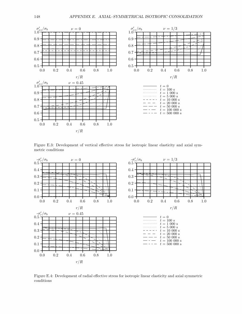
148 APPENDIX E. AXIAL–SYMMETRICAL ISOTROPIC CONSOLIDATION
0.0 0.2 0.4 0.6 0.8 1.0
r/R
0.5
0.6
0.7
0.8
0.9
1.0σ′zz/σb ν = 0
.................................................................................................................................................................................................................................................................................................................................................................................................................................................................................................................................................................
......................................................................................
.....................................................................
........... ........... ........... ........... ........... ........... ........... ........... ........... ........... ........... ........... ........... ........... ........... ........... ........... ........... ........... ........... ........... .......
................ ................ ................ ................ ................ ................ ................ ................ ................ ................ ................ ................ ................ ................ .......
.......................... .......................... .......................... .......................... .......................... .......................... .......................... .......................... .......................... .......................... .......................... .......................... .......
.......................... ........ .......................... ........ .......................... ........ .......................... ........ .......................... ........ .......................... ........ .......................... ........ .......................... ........ .......
.......................... ........ ........ .......................... ........ ........ .......................... ........ ........ .......................... ........ ........ .......................... ........ ........ .......................... ........ ........ .......
0.0 0.2 0.4 0.6 0.8 1.0
r/R
0.5
0.6
0.7
0.8
0.9
1.0σ′zz/σb ν = 1/3
..............................................................................................................................................................................................................................................................................................................................................................................................................................
.......................................................................
...............................................................................................................................
.........................................................................
...................
............................................
......
......
................
........... ........... ........... ........... ........... ........... ........... ........... ........... ........... ........... ........... ........... ......................
......................
......................
......................
............
................ ................ ................ ................ ................ ................ ................................
................................
................................
................
................
................
.......................... .......................... .......................... .......................... .......................... ....................................................
....................................................
...................................................
. .......................... ...........
.......................... ........ .......................... ........ .......................... ........ .......................... ........ .......................... ........ .......................... ........ .......................... ........ .......................... ........ ........
.......................... ........ ........ .......................... ........ ........ .......................... ........ ........ .......................... ........ ........ .......................... ........ ........ .......................... ........ ........ .......
0.0 0.2 0.4 0.6 0.8 1.0
r/R
0.5
0.6
0.7
0.8
0.9
1.0σ′zz/σb ν = 0.45
............................................................................................................................................................................................................................................................................................................................................................................................................................
.....
.....
.....
.....
.....
.....
.....
.....
.....
.....
.....
.....
.....
.....
.....
.....
.....
.....
.....
.....
.....
.....
.....
.
......................................................................................
..........................................................................................................................................
.......................
..................................................................................................
..................
..........................................
.................................
..............
........... ........... ........... ........... ........... ........... ........... ........... ........... ........... ........... ........... ...................... ...........
........... ...........
..................................................................
........... ........... ........... ........... ......
................ ................ ................ ................................
................................
................................
................
................
................
................
................
................
................ ................ ................
.......................... .......................... .......................... .......................... ....................................................
.......................... .......................
... .......................... .....................
..... .......................... .....................
..... .............
.......................... .......................... ................
.......................... ........ .......................... ........ .......................... ........ .......................... ........ .......................... ........ .......................... ........ .......................... ........ .......................... ........ ........
.......................... ........ ..........................
.......................... ........ ........ .......................... ........ ........ .......................... ........ ........ .......................... ........ ........ .......................... ........ ........ .......................... ........ ........ .......
.......................... ........ ........ ................
t = 0t = 100 st = 1 000 st = 5 000 st = 10 000 st = 20 000 st = 50 000 st = 100 000 st = 500 000 s
Figure E.3: Development of vertical effective stress for isotropic linear elasticity and axial sym-metric conditions
0.0 0.2 0.4 0.6 0.8 1.0
r/R
0.0
0.1
0.2
0.3
0.4
0.5-σ′r/σb ν = 0
..........................................................................................................................................................................................................................................................................................................................................................................................................................................................................................................................................................................
.................................................................................................................................................
.......................................................................................................
..............................................................................
........... ........... ........... ........... ........... ........... ........... ........... ........... ........... ........... ........... ........... ......................
......................
......................
......................
......................
...........
................ ................ ................ ................ ................ ................ ................................
................................
................................
................................
.............................
.......................... .......................... .......................... .......................... .......................... .......................... .......................... .......................... .......................... .......................... .......................... .......................... ..........................
.......................... ........ .......................... ........ .......................... ........ .......................... ........ .......................... ........ .......................... ........ .......................... ........ .......................... ........ .......................................... ........ ........ .......................... ........ ........ .......................... ........ ........ .......................... ........ ........ .......................... ........ ........ .......................... ........ ........ .......
0.0 0.2 0.4 0.6 0.8 1.0
r/R
0.0
0.1
0.2
0.3
0.4
0.5-σ′r/σb ν = 1/3
..........................................................................................................................................................................................................................................................................................................................................................................................................................................................................................................................................................................
.................................................................................................................................................
......................................................................................................
.............................................................................
........... ........... ........... ........... ........... ........... ........... ........... ........... ........... ........... ........... ........... ......................
......................
......................
......................
......................
........
................ ................ ................ ................ ................ ................ ................................
................................
................................
................................
.......................
.......................... .......................... .......................... .......................... .......................... .......................... .......................... .......................... .......................... .......................... .......................... .......................... ...................
.......................... ........ .......................... ........ .......................... ........ .......................... ........ .......................... ........ .......................... ........ .......................... ........ .......................... ........ ................................... ........ ........ .......................... ........ ........ .......................... ........ ........ .......................... ........ ........ .......................... ........ ........ .......................... ........ ........ .......
0.0 0.2 0.4 0.6 0.8 1.0
r/R
0.0
0.1
0.2
0.3
0.4
0.5-σ′r/σb ν = 0.45
..........................................................................................................................................................................................................................................................................................................................................................................................................................................................................................................................................................................
......................................................................................
.................................................................................................................................................
.......................
......................................................................................................
..................
.............................................................................
......................... ........... ........... ........... ........... ........... ........... ........... ........... ........... ........... ........... ........... ...........
......................
......................
......................
......................
.................
........... ........... ........... ........... ...................... ................ ................ ................ ................ ................ ................
................................
................................
................................
................................
....
................ ................ ................
.......................... .......................... .......................... .......................... .......................... .......................... .......................... .......................... .......................... .......................... .......................... .......................... ...............
.......................... .......................... ................
.......................... ........ .......................... ........ .......................... ........ .......................... ........ .......................... ........ .......................... ........ .......................... ........ .......................... ........ ........
.......................... ........ ..........................
.......................... ........ ........ .......................... ........ ........ .......................... ........ ........ .......................... ........ ........ .......................... ........ ........ .......................... ........ ........ .......
.......................... ........ ........ ................
t = 0t = 100 st = 1 000 st = 5 000 st = 10 000 st = 20 000 st = 50 000 st = 100 000 st = 500 000 s
Figure E.4: Development of radial effective stress for isotropic linear elasticity and axial symmetricconditions

149
0.0 0.2 0.4 0.6 0.8 1.0
r/R
0.0
0.1
0.2
0.3
0.4
0.5-σ′θ/σb ν = 0
...............................................................................................................................................................................................................................................................................................................................................................................................................................................
..................................................................................................................
......................................................................................
.....................................................................
........... ........... ........... ........... ........... ........... ........... ........... ........... ........... ........... ........... ........... ........... ........... ........... ........... ........... ........... ........... ........... ..........
................ ................ ................ ................ ................ ................ ................ ................ ................ ................ ................ ................ ................ ................ ...........
.......................... .......................... .......................... .......................... .......................... .......................... .......................... .......................... .......................... .......................... .......................... .......................... .................................... ........ .......................... ........ .......................... ........ .......................... ........ .......................... ........ .......................... ........ .......................... ........ .......................... ........ ........
.......................... ........ ........ .......................... ........ ........ .......................... ........ ........ .......................... ........ ........ .......................... ........ ........ .......................... ........ ........ .......
0.0 0.2 0.4 0.6 0.8 1.0
r/R
0.0
0.1
0.2
0.3
0.4
0.5-σ′θ/σb ν = 1/3
.....................................................................................................................................................................................................................................................................................................................................................................................................................................................................................................
................................................................................................................................
.............................................................................................
........................................................................
........... ........... ........... ........... ........... ........... ........... ........... ........... ........... ........... ........... ........... ........... ........... ........... ........... ......................
......................
..................
................ ................ ................ ................ ................ ................ ................ ................ ................................
................................
................................
................
.......................... .......................... .......................... .......................... .......................... .......................... .......................... .......................... .......................... .......................... .......................... .......................... ..............
.......................... ........ .......................... ........ .......................... ........ .......................... ........ .......................... ........ .......................... ........ .......................... ........ .......................... ........ ........
.......................... ........ ........ .......................... ........ ........ .......................... ........ ........ .......................... ........ ........ .......................... ........ ........ .......................... ........ ........ .......
0.0 0.2 0.4 0.6 0.8 1.0
r/R
0.0
0.1
0.2
0.3
0.4
0.5-σ′θ/σb ν = 0.45
................................................................................................................................................................................................................................................................................................................................................................................................................................................................................................................................................
......................................................................................
...........................................................................................................................................
.......................
...................................................................................................
..................
...........................................................................
......................... ........... ........... ........... ........... ........... ........... ........... ........... ........... ........... ........... ........... ...........
......................
........... ......................
......................
......................
........... ........... ........... ........... ...................... ................ ................ ................ ................ ................ ................ ................ ................
................................
................................
................................
................ ................ ................
.......................... .......................... .......................... .......................... .......................... .......................... .......................... .......................... .......................... .......................... .......................... .......................... ..............
.......................... .......................... ................
.......................... ........ .......................... ........ .......................... ........ .......................... ........ .......................... ........ .......................... ........ .......................... ........ .......................... ........ ........
.......................... ........ ..........................
.......................... ........ ........ .......................... ........ ........ .......................... ........ ........ .......................... ........ ........ .......................... ........ ........ .......................... ........ ........ .......
.......................... ........ ........ ................
t = 0t = 100 st = 1 000 st = 5 000 st = 10 000 st = 20 000 st = 50 000 st = 100 000 st = 500 000 s
Figure E.5: Development of tangential effective stress for isotropic linear elasticity and axial sym-metric conditions
0.0 0.2 0.4 0.6 0.8 1.0
r/R
0.7
0.8
0.9
1.0
1.1
1.2
1.3
σzz/σbν = 0
..............................................................................................................................................................................................................................................................................................................................................................................................
.....................................................................................................................................................
............................................................................................................................................
....................................................................................................
.............................................................................
........... ........... ........... ........... ........... ........... ........... ........... ........... ........... ........... ........... ........... ......................
......................
......................
......................
......................
...........
................ ................ ................ ................ ................ ................ ................................
................................
................................
................................
................................
.......................... .......................... .......................... .......................... .......................... .......................... .......................... .......................... .......................... .......................... ....................................................
..........................
.......................... ........ .......................... ........ .......................... ........ .......................... ........ .......................... ........ .......................... ........ .......................... ........ .......................... ........ ..................
.......................... ........ ........ .......................... ........ ........ .......................... ........ ........ .......................... ........ ........ .......................... ........ ........ .......................... ........ ........ .......
0.0 0.2 0.4 0.6 0.8 1.0
r/R
0.7
0.8
0.9
1.0
1.1
1.2
1.3
σzz/σbν = 1/3
........................................................................................................................................................................................................................................................................................................................................................................................................................................................................................
.............................................................................................................................
..........................................................................................
.......................................................................
........... ........... ........... ........... ........... ........... ........... ........... ........... ........... ........... ........... ........... ........... ........... ........... ........... ........... ........... ........... ........... ...........
................ ................ ................ ................ ................ ................ ................ ................ ................ ................ ................ ................ ................ ................ ..............
.......................... .......................... .......................... .......................... .......................... .......................... .......................... .......................... .......................... .......................... .......................... .......................... ..........
.......................... ........ .......................... ........ .......................... ........ .......................... ........ .......................... ........ .......................... ........ .......................... ........ .......................... ........ ........
.......................... ........ ........ .......................... ........ ........ .......................... ........ ........ .......................... ........ ........ .......................... ........ ........ .......................... ........ ........ .......
0.0 0.2 0.4 0.6 0.8 1.0
r/R
0.7
0.8
0.9
1.0
1.1
1.2
1.3
σzz/σbν = 0.45
........................................................................................................................................................................................................................................................................................................................................................................................................................................................
......................................................................................
....................................................................................................................
.......................
......................................................................................
..................
.....................................................................
..............
........... ........... ........... ........... ........... ........... ........... ........... ........... ........... ........... ........... ........... ........... ........... ........... ........... ........... ........... ........... ........... ........
........... ........... ........... ........... ...................... ................ ................ ................ ................ ................ ................ ................ ................ ................ ................ ................ ................ ................ ........
................ ................ ................
.......................... .......................... .......................... .......................... .......................... .......................... .......................... .......................... .......................... .......................... .......................... .......................... ........
.......................... .......................... ................
.......................... ........ .......................... ........ .......................... ........ .......................... ........ .......................... ........ .......................... ........ .......................... ........ .......................... ........ .......
.......................... ........ ..........................
.......................... ........ ........ .......................... ........ ........ .......................... ........ ........ .......................... ........ ........ .......................... ........ ........ .......................... ........ ........ .......
.......................... ........ ........ ................
t = 0t = 100 st = 1 000 st = 5 000 st = 10 000 st = 20 000 st = 50 000 st = 100 000 st = 500 000 s
Figure E.6: Development of vertical total stress for isotropic linear elasticity and axial symmetricconditions
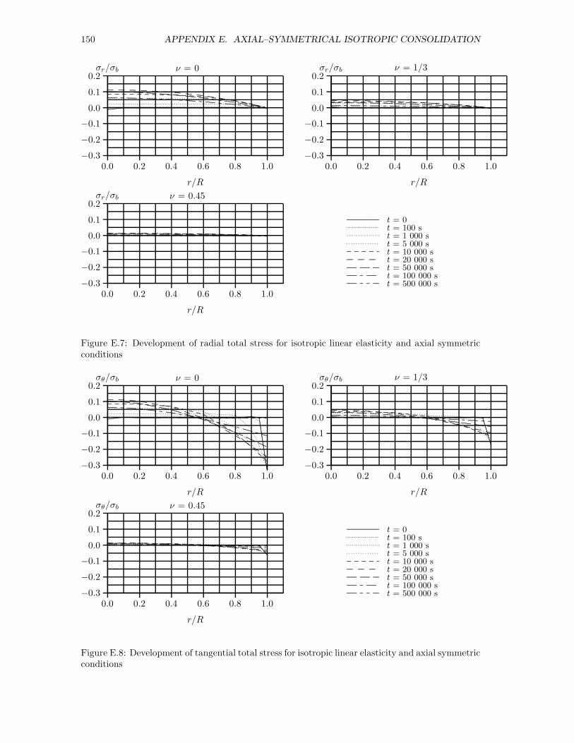
150 APPENDIX E. AXIAL–SYMMETRICAL ISOTROPIC CONSOLIDATION
0.0 0.2 0.4 0.6 0.8 1.0
r/R
−0.3
−0.2
−0.1
0.0
0.1
0.2σr/σb ν = 0
...............................................................................................................................................................................................................................................................................................................................................................................................................................................
..................................................................................................................
......................................................................................
.....................................................................
........... ........... ........... ........... ........... ........... ........... ........... ........... ........... ........... ........... ........... ........... ........... ........... ........... ........... ........... ........... ........... ..........
................ ................ ................ ................ ................ ................ ................ ................ ................ ................ ................ ................ ................ ................ ...........
.......................... .......................... .......................... .......................... .......................... .......................... .......................... .......................... .......................... .......................... .......................... .......................... ..........
.......................... ........ .......................... ........ .......................... ........ .......................... ........ .......................... ........ .......................... ........ .......................... ........ .......................... ........ .................................. ........ ........ .......................... ........ ........ .......................... ........ ........ .......................... ........ ........ .......................... ........ ........ .......................... ........ ........ .......
0.0 0.2 0.4 0.6 0.8 1.0
r/R
−0.3
−0.2
−0.1
0.0
0.1
0.2σr/σb ν = 1/3
.................................................................................................................................................................................................................................................................................................................................................................................................................................................................................................................................................................
......................................................................................
.....................................................................
........... ........... ........... ........... ........... ........... ........... ........... ........... ........... ........... ........... ........... ........... ........... ........... ........... ........... ........... ........... ........... ........
................ ................ ................ ................ ................ ................ ................ ................ ................ ................ ................ ................ ................ ................ ........
.......................... .......................... .......................... .......................... .......................... .......................... .......................... .......................... .......................... .......................... .......................... .......................... ........
.......................... ........ .......................... ........ .......................... ........ .......................... ........ .......................... ........ .......................... ........ .......................... ........ .......................... ........ ................................. ........ ........ .......................... ........ ........ .......................... ........ ........ .......................... ........ ........ .......................... ........ ........ .......................... ........ ........ .......
0.0 0.2 0.4 0.6 0.8 1.0
r/R
−0.3
−0.2
−0.1
0.0
0.1
0.2σr/σb ν = 0.45
...............................................................................................................................................................................................................................................................................................................................................................................................................................................
......................................................................................
..................................................................................................................
.......................
...................................................................................... .......................................................................................
..............
........... ........... ........... ........... ........... ........... ........... ........... ........... ........... ........... ........... ........... ........... ........... ........... ........... ........... ........... ........... ........... .......
........... ........... ........... ........... ......
................ ................ ................ ................ ................ ................ ................ ................ ................ ................ ................ ................ ................ ................ .......
................ ................ ................
.......................... .......................... .......................... .......................... .......................... .......................... .......................... .......................... .......................... .......................... .......................... .......................... .......
.......................... .......................... ................
.......................... ........ .......................... ........ .......................... ........ .......................... ........ .......................... ........ .......................... ........ .......................... ........ .......................... ........ .......
.......................... ........ ..........................
.......................... ........ ........ .......................... ........ ........ .......................... ........ ........ .......................... ........ ........ .......................... ........ ........ .......................... ........ ........ .......
.......................... ........ ........ ................
t = 0t = 100 st = 1 000 st = 5 000 st = 10 000 st = 20 000 st = 50 000 st = 100 000 st = 500 000 s
Figure E.7: Development of radial total stress for isotropic linear elasticity and axial symmetricconditions
0.0 0.2 0.4 0.6 0.8 1.0
r/R
−0.3
−0.2
−0.1
0.0
0.1
0.2σθ/σb ν = 0
..........................................................................................................................................................................................................................................................................................................................................................................................................................................................................................................................................................................
.................................................................................................................................................
.......................................................................................................
..............................................................................
........... ........... ........... ........... ........... ........... ........... ........... ........... ........... ........... ........... ........... ......................
......................
......................
......................
......................
...........
................ ................ ................ ................ ................ ................ ................................
................................
................................
................................
.............................
.......................... .......................... .......................... .......................... .......................... .......................... .......................... .......................... .......................... .......................... .......................... .......................... ..........................
.......................... ........ .......................... ........ .......................... ........ .......................... ........ .......................... ........ .......................... ........ .......................... ........ .......................... ........ ................
.......................... ........ ........ .......................... ........ ........ .......................... ........ ........ .......................... ........ ........ .......................... ........ ........ .......................... ........ ........ .......
0.0 0.2 0.4 0.6 0.8 1.0
r/R
−0.3
−0.2
−0.1
0.0
0.1
0.2σθ/σb ν = 1/3
...................................................................................................................................................................................................................................................................................................................................................................................................................................................................................................
...............................................................................................................................
...........................................................................................
.......................................................................
........... ........... ........... ........... ........... ........... ........... ........... ........... ........... ........... ........... ........... ........... ........... ........... ........... ........... ........... ........... ........... ...........
................ ................ ................ ................ ................ ................ ................ ................ ................ ................ ................ ................ ................ ................ .............
.......................... .......................... .......................... .......................... .......................... .......................... .......................... .......................... .......................... .......................... .......................... .......................... .........
.......................... ........ .......................... ........ .......................... ........ .......................... ........ .......................... ........ .......................... ........ .......................... ........ .......................... ........ ........
.......................... ........ ........ .......................... ........ ........ .......................... ........ ........ .......................... ........ ........ .......................... ........ ........ .......................... ........ ........ .......
0.0 0.2 0.4 0.6 0.8 1.0
r/R
−0.3
−0.2
−0.1
0.0
0.1
0.2σθ/σb ν = 0.45
...........................................................................................................................................................................................................................................................................................................................................................................................................................................................
......................................................................................
.....................................................................................................................
.......................
.......................................................................................
....................................................................................... ..............
........... ........... ........... ........... ........... ........... ........... ........... ........... ........... ........... ........... ........... ........... ........... ........... ........... ........... ........... ........... ........... ........
........... ........... ........... ........... ......
................ ................ ................ ................ ................ ................ ................ ................ ................ ................ ................ ................ ................ ................ ........
................ ................ ................
.......................... .......................... .......................... .......................... .......................... .......................... .......................... .......................... .......................... .......................... .......................... .......................... .......
.......................... .......................... ................
.......................... ........ .......................... ........ .......................... ........ .......................... ........ .......................... ........ .......................... ........ .......................... ........ .......................... ........ .......
.......................... ........ ..........................
.......................... ........ ........ .......................... ........ ........ .......................... ........ ........ .......................... ........ ........ .......................... ........ ........ .......................... ........ ........ .......
.......................... ........ ........ ................
t = 0t = 100 st = 1 000 st = 5 000 st = 10 000 st = 20 000 st = 50 000 st = 100 000 st = 500 000 s
Figure E.8: Development of tangential total stress for isotropic linear elasticity and axial symmetricconditions

151
0.1 1 10 102 103 104 105 106 107
t [s]
−0.6
−0.4
−0.2
0.0
0.2
0.4εr × E/σb r/R = 0.002
..............................................................................................................................................................................................................................................................................................................................................................................................................................................................
............. ............. ............. ............. ............. ............. ............. ............. ............. ............. ............. ............. ..........................
.......................... ............. ............
.......................... ........ .......................... ........ .......................... ........ .......................... ........ .......................... ........ .......................... ........ .......................... ........ ..................
0.1 1 10 102 103 104 105 106 107
t [s]
εr × E/σb r/R = 1.0
...............................................................................................................................................................................................
.........................................
............................................................................................................................................................................
............. ............. ............. ............. ............. ............. ............. ............. ............. ............. ............. ............. ............. ............. ............. ............. ............. .....
.......................... ........ .......................... ........ .......................... ........ .......................... ........ .......................... ........ .......................... ........ .......................... ........ .................
0.1 1 10 102 103 104 105 106 107
t [s]
−0.6
−0.4
−0.2
0.0
0.2
0.4εθ × E/σb r/R = 0.002
..............................................................................................................................................................................................................................................................................................................................................................................................................................................................
............. ............. ............. ............. ............. ............. ............. ............. ............. ............. ............. ............. ..........................
............. ............. ............. ............
.......................... ........ .......................... ........ .......................... ........ .......................... ........ .......................... ........ .......................... ........ .......................... ........ ..........................
0.1 1 10 102 103 104 105 106 107
t [s]
εθ × E/σb r/R = 1.0
................................................................................................................................................................................................................................
..........................................................................................................................................................................................................
............. ............. ............. ............. ............. ............. ............. ............. ............. ............. ............. ..........................
............. ............. ............. ............. .....
.......................... ........ .......................... ........ .......................... ........ .......................... ........ .......................... ........ .......................... ........ .......................... ........ ..........................
0.1 1 10 102 103 104 105 106 107
t [s]
0.2
0.4
0.6
0.8
1.0
1.2εzz × E/σb
................................................................................................................................................................................................................................
..................................................................................................................................................................
.........................................
..............................
............. ............. ............. ............. ............. ............. ............. ............. ............. ............. ............. ..........................
.......................... ............. ............. .............
............. ........
.......................... ........ .......................... ........ .......................... ........ .......................... ........ .......................... ........ .......................... ........ .......................... ........ ..........................
..........................
ν = 0
ν = 1/3
ν = 0.45
Figure E.9: Development of vertical, radial and tangential strain for isotropic linear elasticity andaxial symmetric conditions
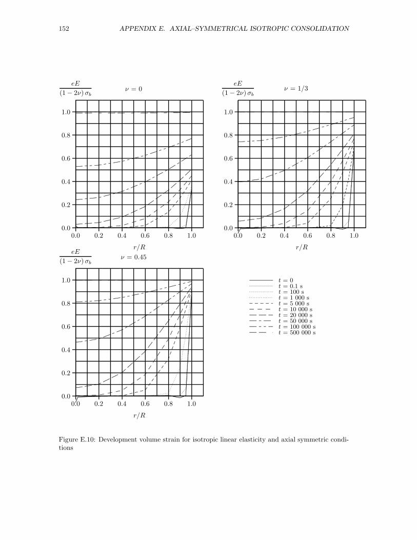
152 APPENDIX E. AXIAL–SYMMETRICAL ISOTROPIC CONSOLIDATION
0.0 0.2 0.4 0.6 0.8 1.0
r/R
0.0
0.2
0.4
0.6
0.8
1.0
eE
(1 − 2ν)σbν = 0
.............................................................................................................................................................................................................................................................................................................................................................................................................................................................................................................................................................................
....................................................................................................................................................
..............................................................................................................
....................................................................................
........... ........... ........... ........... ........... ........... ........... ........... ........... ........... ........... ........... ........... .....................................................................................................................................
................ ................ ................ ................ ................ ................................
................................
................
................
................
................
................
................
................
..............
.......................... .......................... ..............................................
...... .......................... ...........
...............
................................................................................................................................................................................................................
.......................... ........ .......................... ..........................
........ ........ ..........................
.................................. ........
..........................
..................................
..................................
..................................
........
.......................... ........ ........ .......................... ........ ........ ..................................
........ ..........................
................
..........................
................
..........................
................
......................
.......................... .......................... ........... .......................... .......................... ........... .......................... .......................... ........... .......................... .................................................... ........ ........ ........ .......................... ........ ........ ........ .......................... ........ ........ ........ .......................... ........ ........ ........ .......................... ........ ........ .......
0.0 0.2 0.4 0.6 0.8 1.0
r/R
0.0
0.2
0.4
0.6
0.8
1.0
eE
(1 − 2ν)σbν = 1/3
............................................
...................................................................................................................................................................................................................................................................................................................................................................................
....................................................................................................................................................................................................................................................................................................
...................
........................................................................................................................................................................
.........................................................................................................................................
.............. .............. ....... ....... ....... ....... ....... ....... ....... ....... ....... .............. .............. .............. ..................... .............. ....... ....................
.........................................................................................................................................................................
........... ........... ........... ........... ........... ........... ........... ........... ........... ........... ........... ........... .............................................................................................................................................................................................................
................ ................ ................ ................................
................................
................
................
................
................
................
................
................
................
................
................
................
................
................
.......................... .................................................
............................. ............
.............. .........
.....................................................................................................................................................................................................................................................................................
.......................... ........ ..................................
..........................
......................
....................
..........................
..................................
..........................................
..................................
..................................
............
.......................... ........ ........ .......................... ........ ........ .................................. ........ ...................
....... ........ ........................
..................
.......................
...................
........................
..
.......................... .......................... ........... .......................... .......................... ........... .......................... .......................... ........... .......................... ..........................
0.0 0.2 0.4 0.6 0.8 1.0
r/R
0.0
0.2
0.4
0.6
0.8
1.0
eE
(1 − 2ν)σbν = 0.45
..............................................................................................................................................................
................................................................................................................................................................................................................................................................................................................................................................................................................................................................................................................................................................................................................................................................
......................................................................................
.........................................................................
...........................................................................................................................................
.......................
..........................................................................................................................................................
..................
.....................................................
................................................................
..............
........... ........... ........... ........... ........... ........... ........... ........... ........... ......................
......................
....................................................................................................................................................................................................................................
........... ........... ........... ........... ......
................ ................ ................ ................................
................................
................
................
................
................
................
................
................
................
................
................
................
................
................
................
......
................ ................ ................
....................................................
..........................
..........................
..........................
........................................................................................................................................................................................................................................................................................................................
.......................... .......................... ................
.......................... ........ ..................................
.......................... ........
..................................
..........................
..................................
..........................................
..................................
..................................
.............
.......................... ........ ..........................
.......................... ........ ........ .......................... ........ ........ .................................. ........ ......................
.... ........ ........ .......................... ........ ........ ...................
....... ........ ........ ...............
.......................... ........ ........ ................
.......................... .......................... ........... .......................... .......................... ........... .......................... .......................... ........... .......................... ..........................
.......................... .......................... .
t = 0t = 0.1 st = 100 st = 1 000 st = 5 000 st = 10 000 st = 20 000 st = 50 000 st = 100 000 st = 500 000 s
Figure E.10: Development volume strain for isotropic linear elasticity and axial symmetric condi-tions
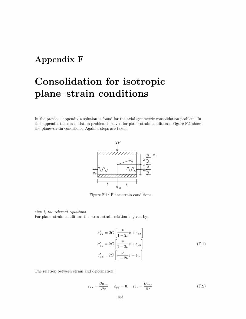
Appendix F
Consolidation for isotropic
plane–strain conditions
In the previous appendix a solution is found for the axial-symmetric consolidation problem. Inthis appendix the consolidation problem is solved for plane–strain conditions. Figure F.1 showsthe plane–strain conditions. Again 4 steps are taken.
...........................................................................................................................................................................................................................................................................................................................................................
.....
.....
....
.....
..............
..............................
............................
............................
................................................
................................................
.....
.....
....
.....
..............
.................................................. ...................
..................................................
...................
..................................................................................................................................................................................................................................................
..................................................................................................................................................................................................................................................
..................................................................................................................................................................................................................................................
..................................................................................................................................................................................................................................................
.....
.....
.....
.....
.....
.....
.....
.....
.....
.....
.....
.....
.....
.....
.....
.....
.....
.....
.....
.....
.....
.....
.....
.....
.....
.....
.....
.....
.....
.....
.....
...
.....
.....
.....
.....
.....
.....
.....
.....
.....
.....
.....
.....
.....
.....
.....
.....
.....
.....
.....
.....
.....
.....
.....
.....
.....
.....
.....
.....
.....
.....
.....
...
.....
.....
.....
.....
.....
.....
.....
.....
.....
.....
.....
.....
.....
.....
.....
.....
.
..............................................................................................................................................................................................................................................................
.............
.............
.....
.....
.....
.....
.....
.....
.....
.....
.....
.....
.....
.....
.....
.....
.....
.....
.....
.....
.....
.....
.....
.....
.....
.....
.....
.....
....
..........................
..........................
..........................
..........................
..........................
..........................
..........................
..........................
..........................
..........................
..........................
..........................
..........................
.........
..........................
..........................
..........................
..........................
..........................
..........................
..........................
..........................
..........................
..........................
..........................
..........................
..........................
.........
..................................................................
................................................................................
.............. .....
.............................................................
................................................................................
..............
.....
.....
.....
.....
.....
.....
.....
.....
.....
.....
.....
.....
.....
.....
.....
.....
.....
.....
.....
.....
.....
.....
.....
.....
.
.....................................................................
..................................................
...................
..................................................
...................
..................................................
...................
.....................................................................
.....................................................................
..................................................
...................
..................................................
...................
..................................................
................... σx
z
xy
2F
l
qx
l
qx
h
Figure F.1: Plane strain conditions
step 1, the relevant equationsFor plane–strain conditions the stress–strain relation is given by:
σ′
xx = 2G
[ν
1 − 2νe+ εxx
]
σ′
yy = 2G
[ν
1 − 2νe+ εyy
]
σ′
zz = 2G
[ν
1 − 2νe+ εzz
](F.1)
The relation between strain and deformation:
εxx =∂uxx∂x
, εyy = 0, εzz =∂uzz∂z
(F.2)
153

154 APPENDIX F. PLANE–STRAIN ISOTROPIC CONSOLIDATION
Equation (F.2) reduces (F.1) to:
σ′
xx = 2G
[ν
1 − 2νe+
∂uxx∂x
]
σ′
yy = 2G
[ν
1 − 2νe
]
σ′
zz = 2G
[ν
1 − 2νe+
∂uzz∂z
](F.3)
The storage equation is given by:k
γw∇2σw =
∂e
∂t(F.4)
Equilibrium of forces gives : (K +
4
3G
)∇2e = ∇2σw (F.5)
Combination of equations (F.4) and (F.5):
∇2e =1
c
∂e
∂t, with c =
k
γw
(K +
4
3G
)(F.6)
step 2, the Laplace transformationEquation (F.6) is solved by the use of the Laplace transformation. Application of the Laplacetransformation to (F.6) gives:
∇2e =1
c(se− e0) (F.7)
In which e0 represents the initial volumetric strain. Since initially the soil behaves undrained itfollows that e0 = 0. For plane–strain condition, εy = 0 and εz is constant in depth:
e = εxx + εzz
∂2εzz∂z2
= 0, ∇2e =∂2εxx∂x2
=∂2e
∂x2, → ∇2e =
∂2e
∂x2
(F.8)
For equation (F.7) is found:∂2e
∂x2− s
ce = 0
standard solution:
e = C1 exp
(√s
cx
)+ C2 exp
(−√s
cx
)
or:
e = C1 cosh
(√s
cx
)+ C2 sinh
(√s
cx
)(F.9)
Equations (F.8) and (F.9) gives:
e = C1 cosh
(√s
cx
)+ C2 sinh
(√s
cx
)=∂uxx∂x
+∂uzz∂z
∂uxx∂x
= C1 cosh
(√s
cx
)+ C2 sinh
(√s
cx
)− ∂uzz
∂z(F.10)
Application of the Laplace transformation to equation (F.5) gives:
∇2e =1
4mG∇2σw, m =
K + 43G
4G=
1 − ν
2 (1 − 2ν)(F.11)
155
Integration of equation (F.11) gives :
e =1
4mGσw + C3, with ∇2C3 = 0 (F.12)
Equation (F.9) and (F.12) give the expression for the pore pressure development in transformedconditions:
σw = 4mG
[C1 cosh
(√s
cx
)+ C2 sinh
(√s
cx
)− C3
](F.13)
Combination of equations (F.9), (F.10) and (F.3) gives the effective stress in transformedconditions. The summation of effective stress and pore pressure, equation (F.13), gives theexpressions for total stress. Note the sign convention in which effective and total stress is definedpositive for tension while pore pressure is defined positive for pressure. The total stress is givenby:
σ = σ′ − σw, → σ = σ′ − σw
The expressions for stress and strain for transformed conditions become:
e = C1 cosh
(√s
cx
)+ C2 sinh
(√s
cx
)(F.14)
∂uxx∂x
= C1 cosh
(√s
cx
)+ C2 sinh
(√s
cx
)− ∂uzz
∂z(F.15)
σw = 4mG
[C1 cosh
(√s
cx
)+ C2 sinh
(√s
cx
)− C3
](F.16)
σ′
xx = 2G
ν
1 − 2ν
(C1 cosh
(√s
cx
)+ C2 sinh
(√s
cx
))+ C1 cosh
(√s
cx
)+
C2 sinh
(√s
cx
)− ∂uzz
∂z
(F.17)
σ′
yy = 2G
[ν
1 − 2ν
(C1 cosh
(√s
cx
)+ C2 sinh
(√s
cx
))](F.18)
σ′
zz = 2G
[ν
1 − 2ν
(C1 cosh
(√s
cx
)+ C2 sinh
(√s
cx
))+∂uzz∂z
](F.19)
σxx = 2GC1
[ν
1 − 2ν+ 1 − 2m
]cosh
(√s
cx
)+ 2GC2
[ν
1 − 2ν+ 1 − 2m
]sinh
(√s
cx
)− 2G
∂uzz∂z
+ 4mGC3
(F.20)
σyy = 2GC1
[ν
1 − 2ν− 2m
]cosh
(√s
cx
)+ 2GC2
[ν
1 − 2ν− 2m
]sinh
(√s
cx
)+
4mGC3
(F.21)
σzz = 2GC1
[ν
1 − 2ν− 2m
]cosh
(√s
cx
)+ 2GC2
[ν
1 − 2ν− 2m
]sinh
(√s
cx
)+
2G∂uzz∂z
+ 4mGC3
(F.22)
step 3, solving for the boundary conditionsThe set of equations (F.14) to (F.22) contains 4 unknown coefficients; C1, C2, C3 and ∂uzz/∂z.These coefficients are to be determined by the boundary conditions:
156 APPENDIX F. PLANE–STRAIN ISOTROPIC CONSOLIDATION
a) at x = 0,∂σw∂x
= 0,→ ∂σw∂x
= 0
b) at x = l, σw = 0,→ σw = 0
c) at x = l, σx = 0,→ σxx = 0
d)l∫
−l
σzz2ldx =
2F
2l,→
l∫
−l
σzz2ldx =
F
l, F =
l∫
0
σzzdx
Boundary condition a and the derivative of equation (F.16) gives:
∂σw∂x
= 4mG
[C1
√s
csinh
(√s
cx
)+ C2
√s
ccosh
(√s
cx
)]
for x = 0:4mG [C1 × 0 + C2 × 1] = 0, C2 = 0 (F.23)
Boundary condition b in combination with equation (F.16) and (F.23) results in:
C3 = C1 cosh
(√s
cl
)(F.24)
Equation (F.16) can now be rewritten in:
σw = 4mGC1
[cosh
(√s
cx
)− cosh
(√s
cl
)](F.25)
Before application of boundary condition c expression (F.20) can now be rewritten:
σxx = 2GC1
[ν
1 − 2ν+ 1 − 2m
]cosh
(√s
cx
)− 2G
∂uzz∂z
+ 4mGC1 cosh
(√s
cl
)
with
[ν
1 − 2ν+ 1 − 2m
]=
[ν
1 − 2ν+
(1 − 2ν)
(1 − 2ν)− 2 (1 − ν)
2 (1 − 2ν)
]= 0
σxx = −2G∂uzz∂z
+ 4mGC1 cosh
(√s
cl
)
with boundary condition c this leads to:
C1 =
∂uzz∂z
2m cosh(√
scl) (F.26)
boundary condition d gives with the equations (F.22), (F.23), (F.24) and (F.26):
F =
l∫
0
2G∂uzz/∂z
2m cosh(√
scl)[
ν
1 − 2ν− 2m
]cosh
(√s
cx
)+ 2G
∂uzz∂z
4mG∂uzz/∂z
2m cosh
(√s
cl
) cosh
(√s
cl
)
dx
F =
l∫
0
2G∂uzz/∂z
2m cosh
(√s
cl
)[
ν
1 − 2ν− 2 (1 − ν)
2 (1 − 2ν)
]cosh
(√s
cx
)+ 4G
∂uzz∂z
dx
F =
l∫
0
−2G
∂uzz∂z
cosh
(√s
cx
)
2m cosh
(√s
cl
) + 4G∂uzz∂z
dx
157
Since ∂uzz/∂z is independent from x it follows:
F =
−2G
∂uzz∂z
sinh
(√s
cx
)
2m
√s
ccosh
(√s
cl
) + 4G∂uzz∂z
x
l
0
F =∂uzz∂z
4Gl−G sinh
(√s
cx
)
m
√s
ccosh
(√s
cl
)
∂uzz∂z
=F
4Gl −G sinh
(√s
cx
)/m
√s
ccosh
(√s
cl
)
F =
∞∫
0
Fe−stdt =1
sF
∂uzz∂z
=F
s
[4Gl−G sinh
(√s
cx
)/m
√s
ccosh
(√s
cl
)] (F.27)
By the expressions (F.23), (F.24), (F.26) and (F.27) the expression of the stresses and strains forthe transformed conditions are determined. The equation (F.14) to (F.22) can now be rewrittenin:
e =
F
2mGcosh
(√s
cx
)
s
[4l− tanh
(√s
cl
)/(√s
cm
)]cosh
(√s
cl
) (F.28)
∂uxx∂x
=
1
G
[F
2mcosh
(√s
cx
)− F cosh
(√s
cl
)]
s
[4l− tanh
(√s
cl
)/(√s
cm
)]cosh
(√s
cl
) (F.29)
σw =
2F
[cosh
(√s
cx
)− cosh
(√s
cl
)]
s
[4l− tanh
(√s
cl
)/(√s
cm
)]cosh
(√s
cl
) (F.30)
σ′
xx =
2F
[cosh
(√s
cx
)− cosh
(√s
cl
)]
s
[4l− tanh
(√s
cl
)/(√s
cm
)]cosh
(√s
cl
) (F.31)
σ′
yy =
2ν
1 − νF cosh
(√s
cx
)
s
[4l− tanh
(√s
cl
)/(√s
cm
)]cosh
(√s
cl
) (F.32)
σ′
zz =
F
[2ν
1 − νcosh
(√s
cx
)+ 2 cosh
(√s
cl
)]
s
[4l − tanh
(√s
cl
)/(√s
cm
)]cosh
(√s
cl
) (F.33)

158 APPENDIX F. PLANE–STRAIN ISOTROPIC CONSOLIDATION
σxx =−2F
s
[4l− tanh
(√s
cl
)/(m
√s
c
)] +2F
s
[4l− tanh
(√s
cl
)/(m
√s
c
)] = 0 (F.34)
σyy =
F
[2 cosh
(√s
cl
)− 1
mcosh
(√s
cx
)]
s
[4l− tanh
(√s
cl
)/(√s
cm
)]cosh
(√s
cl
) (F.35)
σzz =
F
[4 cosh
(√s
cl
)− 1
mcosh
(√s
cx
)]
s
[4l − tanh
(√s
cl
)/(√s
cm
)]cosh
(√s
cl
) (F.36)
step 4, inverse transformationFinding the inverse transforms of the equations above finalises the solution of plane–strainconsolidation problem. The inverse transform is found by using the Heaviside expansion theorem.When elaborating this theorem for the pore pressure development, equation (F.30), it is found:
σw =
m∑
j=1
t (aj)
d
dsn (aj)
eajt
In which:aj = the roots of equation (F.30)t = nominator of equation (F.30)n = denominator of equation (F.30)
The roots of equation (F.30) can be found by:
s = 0 ∨ 4l cosh
(√s
cl
)−
sinh
(√s
cl
)
√s
cm
= 0
For s = 0 also the nominator of (F.30) turns to 0. So s = 0 does not contribute to the inversetransform and is therefore a removable root. The other roots are found by:
4l cosh
(√s
cl
)=
sinh
(√s
cl
)
m
√s
c
m4l
√s
c= tanh
(√s
cl
)
Only for s = 0 a real root is found. For imaginary values trigonometric functions can be written
159
as:
cos (iy) =ei(iy) + e−i(iy)
2=e−y + ey
2= cosh (y)
sin (iy) =ei(iy) − e−i(iy)
2i=e−y − ey
2i
i
i= i
ey − e−y
2= i sinh (y)
sin (iy) = i sinh (y) → sinh (y) =sin (iy)
i
i
i= −i sin (iy)
So:
cosh
(√s
cl
)= cos
(i
√s
cl
)
sinh
(√s
cl
)= −i sin
(i
√s
cl
)
The roots of (F.30) can now be found:
4l cos
(i
√s
cl
)=
−i√scm
sin
(i
√s
cl
)
4m√
scl
−ii
i=
sin(i√
scl)
cos(i√
scl)
4mi
√s
cl = tan
(i
√s
cl
)
with α = i
√s
cl
4mα = tan (α) (F.37)
The values of s that fulfil condition (F.37) are the roots of equation (F.30). Since an infinitenumber of values for s, which fulfil (F.37) can be found, the roots are now indicated by sj and αj .
The next step in deriving the inverse transform of (F.30) is finding the derivative of thedenominator. The derivatives of the individual parts of the denominator are:
d
ds
(√s
cl
)=
l
2
√s
cc
d
dscosh
(√s
cl
)= sinh
(√s
cl
)l
2
√s
cc
d
ds
1√s
cm
=−1
2cm(sc
)1 1
2
d
ds
sinh
(√s
cl
)
√s
cm
= sinh
(√s
cl
)d
ds
1√s
cm
+1√s
cm
d
ds
(sinh
(√s
cl
))=
− sinh
(√s
cl
)
2cm(sc
)1 1
2
+1√s
cm
cosh
(√s
cl
)l
2
√s
cc

160 APPENDIX F. PLANE–STRAIN ISOTROPIC CONSOLIDATION
The derivative of the denominator of (F.30) becomes:
d
ds
[s
(4l cosh
(√s
cl
)− 1
m√
sc
sinh
(√s
cl
))]=
[4l cosh
(√s
cl
)− 1
m√
sc
sinh
(√s
cl
)]d
ds(s) + s
d
ds
4l cosh
(√s
cl
)− 1
m
√s
c
sinh
(√s
cl
)
=
4l cosh
(√s
cl
)− 1
m
√s
c
sinh
(√s
cl
)
+
s
4l sinh
(√s
cl
)l√s
c2c
+
sinh
(√s
cl
)
2cm(sc
)1 1
2
−l cosh
(√s
cl
)
2cs
c
(F.38)
When roots derived by condition (F.37) are applied to (F.38) the first term reduces to zero.Rewriting the second term gives:
2l2 sinh
(√sjcl
)√sjc
+
sinh
(√sjcl
)
2m
√sjc
−l cosh
(√sjcl
)
2m
2l
(√sjcl
)sinh
(√sjcl
)+
l sinh
(√sjcl
)
2m
√sjcl
− l
2mcosh
(√sjcl
)
with: i
√sjcl = αj , →
√sjcl = −αji
−2lαji sinh (−αji) +l sinh (−αji)2m (−αji)
− l
2mcosh (−αji)
with: sinh (−αji) = i sin (−αj) and
cosh (−αji) = cos (−αj)
−2lαji i sin (−αj) −li sin (−αj)
2mαji− l
2mcos (−αj) =
2lαj sin (−αj) −l
2mαjsin (−αj) −
l
2mcos (−αj) =
−2lαj sin (αj) +l
2mαjsin (αj) −
l
2mcos (αj)
l sin (αj)
(1
2mαj− 2αj
)− l
2mcos (αj) (F.39)
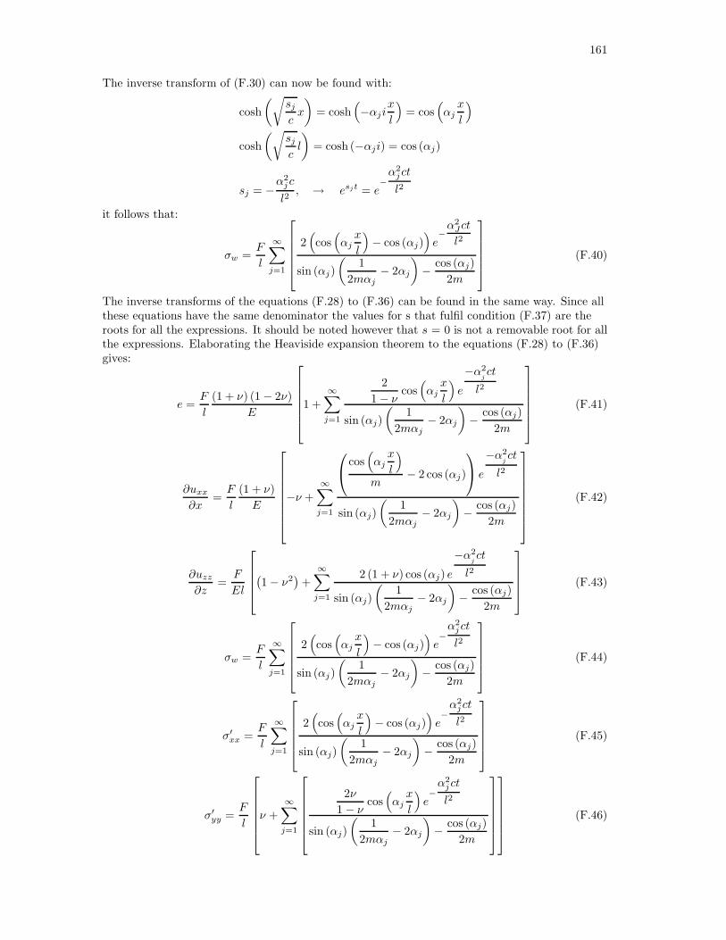
161
The inverse transform of (F.30) can now be found with:
cosh
(√sjcx
)= cosh
(−αji
x
l
)= cos
(αjx
l
)
cosh
(√sjcl
)= cosh (−αji) = cos (αj)
sj = −α2jc
l2, → esjt = e
−
α2jct
l2
it follows that:
σw =F
l
∞∑
j=1
2(cos(αjx
l
)− cos (αj)
)e−
α2Jct
l2
sin (αj)
(1
2mαj− 2αj
)− cos (αj)
2m
(F.40)
The inverse transforms of the equations (F.28) to (F.36) can be found in the same way. Since allthese equations have the same denominator the values for s that fulfil condition (F.37) are theroots for all the expressions. It should be noted however that s = 0 is not a removable root for allthe expressions. Elaborating the Heaviside expansion theorem to the equations (F.28) to (F.36)gives:
e =F
l
(1 + ν) (1 − 2ν)
E
1 +
∞∑
j=1
2
1 − νcos(αjx
l
)e
−α2jct
l2
sin (αj)
(1
2mαj− 2αj
)− cos (αj)
2m
(F.41)
∂uxx∂x
=F
l
(1 + ν)
E
−ν +
∞∑
j=1
cos(αjx
l
)
m− 2 cos (αj)
e
−α2jct
l2
sin (αj)
(1
2mαj− 2αj
)− cos (αj)
2m
(F.42)
∂uzz∂z
=F
El
(1 − ν2
)+
∞∑
j=1
2 (1 + ν) cos (αj) e
−α2jct
l2
sin (αj)
(1
2mαj− 2αj
)− cos (αj)
2m
(F.43)
σw =F
l
∞∑
j=1
2(cos(αjx
l
)− cos (αj)
)e−
α2jct
l2
sin (αj)
(1
2mαj− 2αj
)− cos (αj)
2m
(F.44)
σ′
xx =F
l
∞∑
j=1
2(cos(αjx
l
)− cos (αj)
)e−
α2jct
l2
sin (αj)
(1
2mαj− 2αj
)− cos (αj)
2m
(F.45)
σ′
yy =F
l
ν +
∞∑
j=1
2ν
1 − νcos(αjx
l
)e−
α2jct
l2
sin (αj)
(1
2mαj− 2αj
)− cos (αj)
2m
(F.46)

162 APPENDIX F. PLANE–STRAIN ISOTROPIC CONSOLIDATION
σ′
zz =F
l
1 +
∞∑
j=1
2
(ν
1 − νcos(αjx
l
)+ cos (αj)
)e−
α2jct
l2
sin (αj)
(1
2mαj− 2αj
)− cos (αj)
2m
(F.47)
σxx = 0 (F.48)
σyy =F
l
ν +
∞∑
j=1
(2 cos (αj) −
1
mcos(αjx
l
))e−
α2jct
l2
sin (αj)
(1
2mαj− 2αj
)− cos (αj)
2m
(F.49)
σzz =F
l
1 +
∞∑
j=1
(4 cos (αj) −
1
mcos(αjx
l
))e−
α2jct
l2
sin (αj)
(1
2mαj− 2αj
)− cos (αj)
2m
(F.50)
As is to be expected, the derivation of the inverse transforms of the expressions for total stressleads to the same results as the summation of the expressions for effective stress (F.45) to (F.47)and the expression for the pore pressure development (F.44). The same holds for the expressionof the volumetric strain, which can either be found by the inverse transform of (F.28) or by thesummation of (F.42) and (F.43).
Function f(t)
Equivalent to appendix E an expression for the function f(t) can be derived. With equations(F.5), (F.12) and (F.13) the following is found:
f(t) =F
l+F
l
∞∑
j=1
2 cos(αj)e
−α2jct
l2
sin(αj)
(1
2mαj− 2αj
)− l
2m cos(αj)
(F.51)

163
Graphs of stress and strain
To illustrate the results this section presents graphs of the derived expressions for stress and strain.The graphs present the stress and strain for c = 1 ×10⁻⁶ m2/s and L = 1.0 m.
0.0 0.2 0.4 0.6 0.8 1.00.0
0.1
0.2
0.3
0.4
0.5
0.6
-σw × l/F
x/l
ν = 0
......................................................................................................................................................................................................................................................................................................................................................................................................................................................................................................................................................................................................................
.............................................................................................................................................................
..................................................................................................................
.......................................................................................
........... ........... ........... ........... ........... ........... ........... ........... ........... ........... ........... ........... ........... ........... ........... ......................
.............................................................................................................
................ ................ ................ ................ ................ ................ ................ ................ ................................
................................
................
................
................
................
................
......
.......................... .......................... .......................... .......................... .......................... .......................... .......................... ....................................................
....................................................
....................................................
....................................
.......................... ........ .......................... ........ .......................... ........ .......................... ........ ..................................
..................................
..................................
..................................
..................................
................
.......................... ........ ........ .......................... ........ ........ .......................... ........ ........ .......................... ........ ........ .......................... ........ ........ .......................... ................
..........................
.......................... .......................... ........ .......................... .......................... ........ .......................... .......................... ........ .......................... .......................... ........ .......................... .......................... .............. ...... ...... ...... ...... ...... ...... ...... ...... ...... ...... ...... ...... ...... ...... ...... ...... ...... ...... ...... ...... ......
0.0 0.2 0.4 0.6 0.8 1.00.0
0.1
0.2
0.3
0.4
0.5
0.6
-σw × l/F
x/l
ν = 1/3
......................................................................................................................................................................................................................................................................................................................................................................................................................................................................................................................................................................................................................
............................................................................................................................................................
..................................................................................................................
.......................................................................................
........... ........... ........... ........... ........... ........... ........... ........... ........... ........... ........... ........... ........... ........... ........... ......................
.................................
.......................................................................
................ ................ ................ ................ ................ ................ ................ ................ ................................
................................
................
................
................
................
................
.......................... .......................... .......................... .......................... .......................... .......................... .......................... ....................................................
....................................................
....................................................
...........................
.......................... ........ .......................... ........ .......................... ........ .......................... ........ .......................... ..................................
..................................
..................................
..................................
..............
.......................... ........ ........ .......................... ........ ........ .......................... ........ ........ .......................... ........ ........ .......................... ........ ........ .......................... ........ ........ ...................
.......................... .......................... ........ .......................... .......................... ........ .......................... .......................... ........ .......................... .......................... ........ .......................... .......................... .............. ...... ...... ...... ...... ...... ...... ...... ...... ...... ...... ...... ...... ...... ...... ...... ...... ...... ...... ...... ...... ......
0.0 0.2 0.4 0.6 0.8 1.00.0
0.1
0.2
0.3
0.4
0.5
0.6
-σw × l/Fν = 0.45
x/l
......................................................................................................................................................................................................................................................................................................................................................................................................................................................................................................................................................................................................................
......................................................................................
............................................................................................................................................................
.......................
..................................................................................................................
..........................................................................
..............................
..............
........... ........... ........... ........... ........... ........... ........... ........... ........... ........... ........... ........... ........... ........... ........... ......................
......................................................................................................
........... ........... ........... ........... ......
................ ................ ................ ................ ................ ................ ................ ................ ................................
................................
................
................
................
................
................
................ ................ ................
.......................... .......................... .......................... .......................... .......................... .......................... .......................... ....................................................
....................................................
....................................................
..........................
.......................... .......................... ................
.......................... ........ .......................... ........ .......................... ........ .......................... ........ .......................... ........ ..................................
..................................
..................................
..................................
.......................... ........ .................................................... ........ ........ .......................... ........ ........ .......................... ........ ........ .......................... ........ ........ .......................... ........ ........ .......................... ........ ........ ...............
.......................... ........ ........ ................
.......................... .......................... ........ .......................... .......................... ........ .......................... .......................... ........ .......................... .......................... ........ .......................... .......................... ........
.......................... .......................... ........
...... ...... ...... ...... ...... ...... ...... ...... ...... ...... ...... ...... ...... ...... ...... ...... ...... ...... ...... ...... ...... ...... ...... ...... ...... ...... ......
t = 0t = 100 st = 1 000 st = 5 000 st = 10 000 st = 20 000 st = 50 000 st = 100 000 st = 500 000 st = 1 000 000 st = 5 000 000 s
Figure F.2: Pore pressure development for plane strain conditions and isotropic linear elasticity
0.0 0.2 0.4 0.6 0.8 1.00.4
0.5
0.6
0.7
0.8
0.9
1.0
σ′zz × l/F ν = 0
x/l
....................................................................................................................................................................................................................................................................................................................................................................................................................................................................................................................................................................................................................................................................................................................................... ........... ........... ........... ........... ........... ........... ........... ........... ........... ........... ........... ........... ........... ........... ........... ........... ........... ........... ........... ........... .......
................ ................ ................ ................ ................ ................ ................ ................ ................ ................ ................ ................ ................ ................ .......
.......................... .......................... .......................... .......................... .......................... .......................... .......................... .......................... .......................... .......................... .......................... .......................... .......
.......................... ........ .......................... ........ .......................... ........ .......................... ........ .......................... ........ .......................... ........ .......................... ........ .......................... ........ .......
.......................... ........ ........ .......................... ........ ........ .......................... ........ ........ .......................... ........ ........ .......................... ........ ........ .......................... ........ ........ .......
.......................... .......................... ........ .......................... .......................... ........ .......................... .......................... ........ .......................... .......................... ........ .......................... .......................... .......
...... ...... ...... ...... ...... ...... ...... ...... ...... ...... ...... ...... ...... ...... ...... ...... ...... ...... ...... ...... ...... ......
0.0 0.2 0.4 0.6 0.8 1.00.4
0.5
0.6
0.7
0.8
0.9
1.0
σ′zz × l/F ν = 1/3
x/l
.........................................................................................................................................................................................................................................................................................................................................................................................................................................................................................................................
.....................................................................................................................................
.................................................................................................
...........................................................................
........... ........... ........... ........... ........... ........... ........... ........... ........... ........... ........... ........... ........... ........... ........... ......................
..................................................................
................ ................ ................ ................ ................ ................ ................ ................ ................ ................................
................
................
................
................
...
.......................... .......................... .......................... .......................... .......................... .......................... .......................... ....................
......................
.................................... ..........
................
..........................
.........................
.......................... ........ .......................... ........ .......................... ........................
.......... ........ .......................... ........ ................
..................
..........................
.....................
............. ........
......................
.......................... ........ ........ .......................... ........ ........ .......................... ........ ........ .......................... ........ ........ ..........................
........ ........ .................................. ........ ..................................... .......................... ........ .......................... .......................... ........ .......................... .......................... ........ .......................... .......................... ........ .......................... .......................... ........
...... ...... ...... ...... ...... ...... ...... ...... ...... ...... ...... ...... ...... ...... ...... ...... ...... ...... ...... ...... ...... ......
0.0 0.2 0.4 0.6 0.8 1.00.4
0.5
0.6
0.7
0.8
0.9
1.0
σ′zz × l/F
ν = 0.45
x/l
....................................................................................................................................................................................................................................................................................................................................................................................................................................................................................................................................................................................
......................................................................................
....................................................................................................................................................
.......................
...........................................................................................................
..................
........................................................
..........................
..............
........... ........... ........... ........... ........... ........... ........... ........... ........... ........... ........... ........... ........... ........... ........... ......................
........................................................................................
........... ........... ........... ........... ......
................ ................ ................ ................ ................ ................ ................ ................ ................................
................
................
................................
................
................
....
................ ................ ................
.......................... .......................... .......................... .......................... .......................... .......................... .................
........................
...............................................................
............................................................................................
.......................... .......................... ................
.......................... ........ .......................... ........ .................................. ....................
...... ......................
....................
..........................
..................................
..................................
..................................
...
.......................... ........ ..........................
.......................... ........ ........ .......................... ........ ........ .......................... ........ ........ .................................. ........ ........................
.. ........ ........ .......................... ........ ........ ............
.......................... ........ ........ ................
.......................... .......................... ........ .......................... .......................... ........ .......................... .......................... ........ .......................... .......................... ........ .......................... .......................... ........
.......................... .......................... ........
...... ...... ...... ...... ...... ...... ...... ...... ...... ...... ...... ...... ...... ...... ...... ...... ...... ...... ...... ...... ...... ......
...... ...... ...... ...... ......
t = 0t = 100 st = 1 000 st = 5 000 st = 10 000 st = 20 000 st = 50 000 st = 100 000 st = 500 000 st = 1 000 000 st = 5 000 000 s
Figure F.3: Development of vertical effective stress for plane strain conditions and isotropic linearelasticity

164 APPENDIX F. PLANE–STRAIN ISOTROPIC CONSOLIDATION
0.0 0.2 0.4 0.6 0.8 1.00.0
0.1
0.2
0.3
0.4
0.5
0.6
-σ′xx × l/F
ν = 0
x/l
......................................................................................................................................................................................................................................................................................................................................................................................................................................................................................................................................................................................................................
.............................................................................................................................................................
..................................................................................................................
.......................................................................................
........... ........... ........... ........... ........... ........... ........... ........... ........... ........... ........... ........... ........... ........... ........... ......................
.............................................................................................................
................ ................ ................ ................ ................ ................ ................ ................ ................................
................................
................
................
................
................
................
......
.......................... .......................... .......................... .......................... .......................... .......................... .......................... ....................................................
....................................................
....................................................
....................................
.......................... ........ .......................... ........ .......................... ........ .......................... ........ ..................................
..................................
..................................
..................................
..................................
................
.......................... ........ ........ .......................... ........ ........ .......................... ........ ........ .......................... ........ ........ .......................... ........ ........ .......................... ................
..........................
.......................... .......................... ........ .......................... .......................... ........ .......................... .......................... ........ .......................... .......................... ........ .......................... .......................... .............. ...... ...... ...... ...... ...... ...... ...... ...... ...... ...... ...... ...... ...... ...... ...... ...... ...... ...... ...... ...... ......
0.0 0.2 0.4 0.6 0.8 1.00.0
0.1
0.2
0.3
0.4
0.5
0.6
-σ′xx × l/F
ν = 1/3
x/l
......................................................................................................................................................................................................................................................................................................................................................................................................................................................................................................................................................................................................................
............................................................................................................................................................
..................................................................................................................
.......................................................................................
........... ........... ........... ........... ........... ........... ........... ........... ........... ........... ........... ........... ........... ........... ........... ......................
........................................................................................................
................ ................ ................ ................ ................ ................ ................ ................ ................................
................................
................
................
................
................
................
.......................... .......................... .......................... .......................... .......................... .......................... .......................... ....................................................
....................................................
....................................................
...........................
.......................... ........ .......................... ........ .......................... ........ .......................... ........ ..................................
..................................
..................................
..................................
..................................
......
.......................... ........ ........ .......................... ........ ........ .......................... ........ ........ .......................... ........ ........ .......................... ........ ........ .......................... ........ ........ ...................
.......................... .......................... ........ .......................... .......................... ........ .......................... .......................... ........ .......................... .......................... ........ .......................... .......................... .............. ...... ...... ...... ...... ...... ...... ...... ...... ...... ...... ...... ...... ...... ...... ...... ...... ...... ...... ...... ...... ......
0.0 0.2 0.4 0.6 0.8 1.00.0
0.1
0.2
0.3
0.4
0.5
0.6
-σ′xx × l/F
ν = 0.45
x/l
......................................................................................................................................................................................................................................................................................................................................................................................................................................................................................................................................................................................................................
......................................................................................
............................................................................................................................................................
.......................
..................................................................................................................
..........................................................................
..............................
..............
........... ........... ........... ........... ........... ........... ........... ........... ........... ........... ........... ........... ........... ........... ........... ......................
......................
................................................................................
........... ........... ........... ........... ......
................ ................ ................ ................ ................ ................ ................ ................ ................................
................................
................
................
................
................
................
................ ................ ................
.......................... .......................... .......................... .......................... .......................... .......................... .......................... ....................................................
....................................................
....................................................
..........................
.......................... .......................... ................
.......................... ........ .......................... ........ .......................... ........ .......................... ........ .......................... ..................................
..................................
..................................
..................................
........
.......................... ........ .................................................... ........ ........ .......................... ........ ........ .......................... ........ ........ .......................... ........ ........ .......................... ........ ........ .......................... ........ ........ ...............
.......................... ........ ........ ................
.......................... .......................... ........ .......................... .......................... ........ .......................... .......................... ........ .......................... .......................... ........ .......................... .......................... ........
.......................... .......................... ........
...... ...... ...... ...... ...... ...... ...... ...... ...... ...... ...... ...... ...... ...... ...... ...... ...... ...... ...... ...... ...... ...... ...... ...... ...... ...... ......
t = 0t = 100 st = 1 000 st = 5 000 st = 10 000 st = 20 000 st = 50 000 st = 100 000 st = 500 000 st = 1 000 000 st = 5 000 000 s
Figure F.4: Development effective stress in x-direction for plane strain conditions and isotropiclinear elasticity
0.0 0.2 0.4 0.6 0.8 1.00.0
0.1
0.2
0.3
0.4
0.5
-σ′yy × l/F
ν = 0
x/l
...........................................................................................................................................................................................................................................................................................................................................................................................................................................
0.0 0.2 0.4 0.6 0.8 1.00.0
0.1
0.2
0.3
0.4
0.5
-σ′yy × l/F
ν = 1/3
x/l
............................................................................................................................................................................................................................................................................................................................................................................................................................................................................................................................................
..........................................................................................................................................
....................................................................................................
.............................................................................
........... ........... ........... ........... ........... ........... ........... ........... ........... ........... ........... ........... ........... ........... ........... ......................
.............................................................................
................ ................ ................ ................ ................ ................ ................ ................ ................................
................
................
................
................................
............
.......................... .......................... .......................... .......................... .......................... ...............................................
..... ..........................
..........................
..........................
..........................
..........................
..........................
.......................... ........ .......................... ........ .................................. .........................
. ........ ..........................
......................
....................
.......................... ........
..................................
..........................
.......................... ........ ........ .......................... ........ ........ .......................... ........ ........ .................................. ........ ..........................
........ ........ .......................... ........ ........ ...........
.......................... .......................... ........ .......................... .......................... ........ .......................... .......................... ........ .......................... .......................... ........ .......................... .......................... ........
...... ...... ...... ...... ...... ...... ...... ...... ...... ...... ...... ...... ...... ...... ...... ...... ...... ...... ...... ...... ...... ......
0.0 0.2 0.4 0.6 0.8 1.00.0
0.1
0.2
0.3
0.4
0.5
-σ′yy × l/F
ν = 0.45
x/l
..................................................................................................................................................................................................................................................................................................................................................................................................................................................................................................................................................................................................................
......................................................................................
............................................................................................................................................................
.......................
................................................................................................................. ..................
........................................................
..............................
..............
........... ........... ........... ........... ........... ........... ........... ........... ........... ........... ........... ........... ........... ........... ........... .........................................................................................................................
........... ........... ........... ........... ......
................ ................ ................ ................ ................ ................ ................ ................ .............................
...................
................
................
................
................
................
................
................ ................ ................
.......................... .......................... .......................... .......................... .............................................
....... ..........................
....................................................
..................................................................................................................................
.......................... .......................... ................
.......................... ........ .......................... ........ .................................. .................
.................
..................................
..........................
..................................
..........................................
..................................
.......................... ........ ..........................
.......................... ........ ........ .......................... ........ ........ .................................. ........ .......................
... ........ ........ .......................... ........ ........ .................
.................
.......................
.......................... ........ ........ ................
.......................... .......................... ........ .......................... .......................... ........ .......................... .......................... ........ .......................... .......................... ........ .......................... .......................... ........
.......................... .......................... ........
...... ...... ...... ...... ...... ...... ...... ...... ...... ...... ...... ...... ...... ...... ...... ...... ...... ...... ...... ...... ...... ......
...... ...... ...... ...... ......
t = 0t = 100 st = 1 000 st = 5 000 st = 10 000 st = 20 000 st = 50 000 st = 100 000 st = 500 000 st = 1 000 000 st = 5 000 000 s
Figure F.5: Development effective stress in y-direction for plane strain conditions and isotropiclinear elasticity
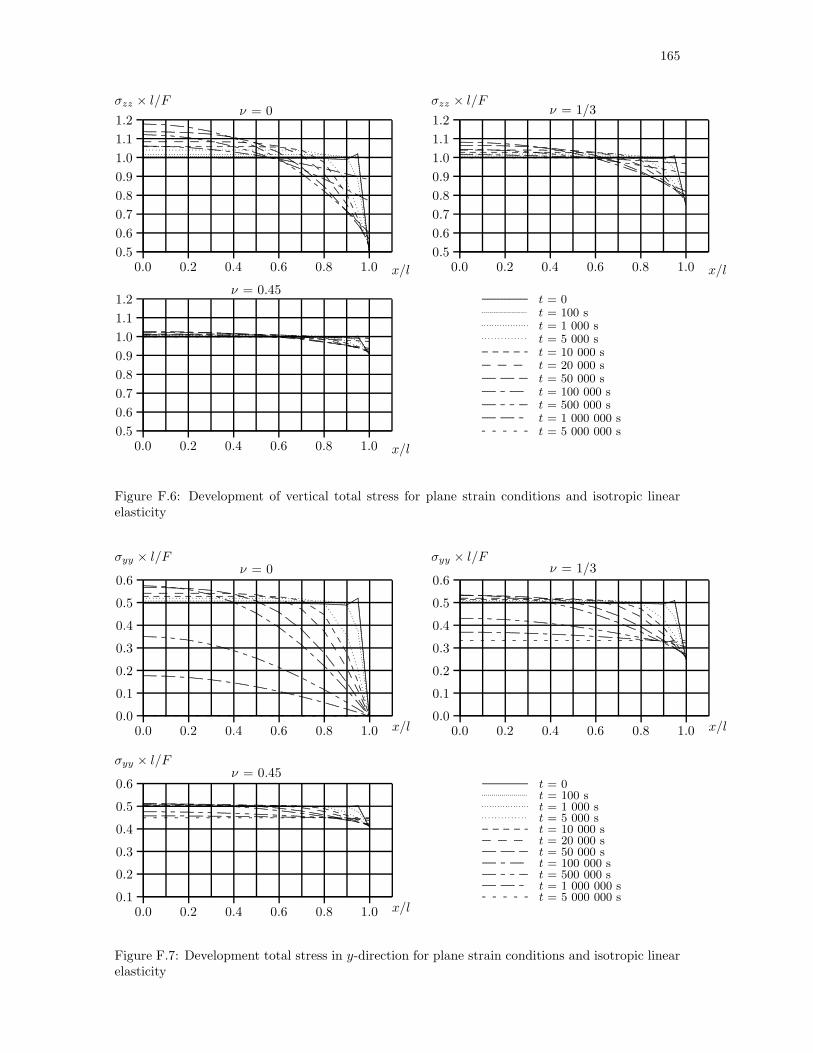
165
0.0 0.2 0.4 0.6 0.8 1.00.5
0.6
0.7
0.8
0.9
1.0
1.1
1.2
σzz × l/Fν = 0
x/l
......................................................................................................................................................................................................................................................................................................................................................................................................................................................................................................................................................................................................................
.............................................................................................................................................................
..................................................................................................................
.......................................................................................
........... ........... ........... ........... ........... ........... ........... ........... ........... ........... ........... ........... ........... ........... ........... ......................
.............................................................................................................
................ ................ ................ ................ ................ ................ ................ ................ ................................
................................
................
................
................
................
................
......
.......................... .......................... .......................... .......................... .......................... .......................... .......................... ....................................................
....................................................
....................................................
....................................
.......................... ........ .......................... ........ .......................... ........ .......................... ........ ..................................
..................................
..................................
..................................
..................................
................
.......................... ........ ........ .......................... ........ ........ .......................... ........ ........ .......................... ........ ........ .......................... ........ ........ .......................... ................
..........................
.......................... .......................... ........ .......................... .......................... ........ .......................... .......................... ........ .......................... .......................... ........ .......................... .......................... ........
...... ...... ...... ...... ...... ...... ...... ...... ...... ...... ...... ...... ...... ...... ...... ...... ...... ...... ...... ...... ...... ......
0.0 0.2 0.4 0.6 0.8 1.00.5
0.6
0.7
0.8
0.9
1.0
1.1
1.2
σzz × l/Fν = 1/3
x/l
.........................................................................................................................................................................................................................................................................................................................................................................................................................................................................................................................
.....................................................................................................................................
.................................................................................................
...........................................................................
........... ........... ........... ........... ........... ........... ........... ........... ........... ........... ........... ........... ........... ........... ........... ........... ........... ......................
......................
......................
................ ................ ................ ................ ................ ................ ................ ................ ................ ................ ................................
................................
...................
.......................... .......................... .......................... .......................... .......................... .......................... .......................... .......................... .......................... .......................... ....................................................
.........................
.......................... ........ .......................... ........ .......................... ........ .......................... ........ .......................... ........ .......................... ........ .......................... ........ .......................... ........ .....................
.......................... ........ ........ .......................... ........ ........ .......................... ........ ........ .......................... ........ ........ .......................... ........ ........ .......................... ........ ........ ..........
.......................... .......................... ........ .......................... .......................... ........ .......................... .......................... ........ .......................... .......................... ........ .......................... .......................... ........
...... ...... ...... ...... ...... ...... ...... ...... ...... ...... ...... ...... ...... ...... ...... ...... ...... ...... ...... ...... ...... ......
0.0 0.2 0.4 0.6 0.8 1.00.5
0.6
0.7
0.8
0.9
1.0
1.1
1.2ν = 0.45
x/l
.................................................................................................................................................................................................................................................................................................................................................................................................................................................................
......................................................................................
.......................................................................................................................
.......................
........................................................................................
..................
......................................................................
......................... ........... ........... ........... ........... ........... ........... ........... ........... ........... ........... ........... ........... ........... ........... ........... ........... ........... ........... ........... ........... ........... ........... ........... ........... ........... ......
................ ................ ................ ................ ................ ................ ................ ................ ................ ................ ................ ................ ................ ................ ...........
................ ................ ................
.......................... .......................... .......................... .......................... .......................... .......................... .......................... .......................... .......................... .......................... .......................... .......................... ..........
.......................... .......................... ................
.......................... ........ .......................... ........ .......................... ........ .......................... ........ .......................... ........ .......................... ........ .......................... ........ .......................... ........ .........
.......................... ........ ..........................
.......................... ........ ........ .......................... ........ ........ .......................... ........ ........ .......................... ........ ........ .......................... ........ ........ .......................... ........ ........ ........
.......................... ........ ........ ................
.......................... .......................... ........ .......................... .......................... ........ .......................... .......................... ........ .......................... .......................... ........ .......................... .......................... .......
.......................... .......................... ........
...... ...... ...... ...... ...... ...... ...... ...... ...... ...... ...... ...... ...... ...... ...... ...... ...... ...... ...... ...... ...... ......
...... ...... ...... ...... ......
t = 0t = 100 st = 1 000 st = 5 000 st = 10 000 st = 20 000 st = 50 000 st = 100 000 st = 500 000 st = 1 000 000 st = 5 000 000 s
Figure F.6: Development of vertical total stress for plane strain conditions and isotropic linearelasticity
0.0 0.2 0.4 0.6 0.8 1.00.0
0.1
0.2
0.3
0.4
0.5
0.6
σyy × l/Fν = 0
x/l
............................................................................................................................................................................................................................................................................................................................................................................................................................................................................................................................................................................................................................................................
......................................................................................................................................................................
.........................................................................................................................
............................................................................................
........... ........... ........... ........... ........... ........... ........... ........... ........... ........... ........... ........... ........... ........... ........... ......................
..........................................................................................................................
................ ................ ................ ................ ................ ................ ................ ................ ................................
................................
................
................
................
................
................
................
......
.......................... .......................... .......................... .......................... .......................... .......................... ....................................................
....................................................
....................................................
....................................................
...........................
.......................... ........ .......................... ........ .......................... ........ ..................................
..................................
..................................
..................................
..................................
............................................................
.....
.......................... ........ ........ .......................... ........ ........ .......................... ........ ........ .......................... ........ .................................. ........
..................................
................
..............................
.......................... .......................... ........ .......................... .......................... ........ .......................... .......................... ........ .......................... .......................... ........ .......................... .......................... .............. ...... ...... ...... ...... ...... ...... ...... ...... ...... ...... ...... ...... ...... ...... ...... ...... ...... ...... ...... ...... ......
0.0 0.2 0.4 0.6 0.8 1.00.0
0.1
0.2
0.3
0.4
0.5
0.6
σyy × l/Fν = 1/3
x/l
............................................................................................................................................................................................................................................................................................................................................................................................................................................................................................................................................
..........................................................................................................................................
....................................................................................................
.............................................................................
........... ........... ........... ........... ........... ........... ........... ........... ........... ........... ........... ........... ........... ........... ........... ........... ........... ......................
......................
.................................
................ ................ ................ ................ ................ ................ ................ ................ ................ ................ ................................
................................
................
............
.......................... .......................... .......................... .......................... .......................... .......................... .......................... .......................... .......................... .......................... ....................................................
..........................
.......................... ........ .......................... ........ .......................... ........ .......................... ........ .......................... ........ .......................... ........ .......................... ........ .......................... ..................................
.......................... ........ ........ .......................... ........ ........ .......................... ........ ........ .......................... ........ ........ .......................... ........ ........ .......................... ........ ........ ...........
.......................... .......................... ........ .......................... .......................... ........ .......................... .......................... ........ .......................... .......................... ........ .......................... .......................... .............. ...... ...... ...... ...... ...... ...... ...... ...... ...... ...... ...... ...... ...... ...... ...... ...... ...... ...... ...... ...... ......
0.0 0.2 0.4 0.6 0.8 1.00.1
0.2
0.3
0.4
0.5
0.6
σyy × l/Fν = 0.45
x/l
.......................................................................................................................................................................................................................................................................................................................................................................................................................................................................
......................................................................................
........................................................................................................................
.......................
.........................................................................................
........................................................................................
..............
........... ........... ........... ........... ........... ........... ........... ........... ........... ........... ........... ........... ........... ........... ........... ........... ........... ........... ........... ........... ......................
........... ........... ........... ........... ......
................ ................ ................ ................ ................ ................ ................ ................ ................ ................ ................ ................ ................ ............................
................ ................ ................
.......................... .......................... .......................... .......................... .......................... .......................... .......................... .......................... .......................... .......................... .......................... .......................... ...........
.......................... .......................... ................
.......................... ........ .......................... ........ .......................... ........ .......................... ........ .......................... ........ .......................... ........ .......................... ........ .......................... ........ ..........
.......................... ........ ..........................
.......................... ........ ........ .......................... ........ ........ .......................... ........ ........ .......................... ........ ........ .......................... ........ ........ .......................... ........ ........ ........
.......................... ........ ........ ................
.......................... .......................... ........ .......................... .......................... ........ .......................... .......................... ........ .......................... .......................... ........ .......................... .......................... .......
.......................... .......................... ........
...... ...... ...... ...... ...... ...... ...... ...... ...... ...... ...... ...... ...... ...... ...... ...... ...... ...... ...... ...... ...... ......
...... ...... ...... ...... ......
t = 0t = 100 st = 1 000 st = 5 000 st = 10 000 st = 20 000 st = 50 000 st = 100 000 st = 500 000 st = 1 000 000 st = 5 000 000 s
Figure F.7: Development total stress in y-direction for plane strain conditions and isotropic linearelasticity
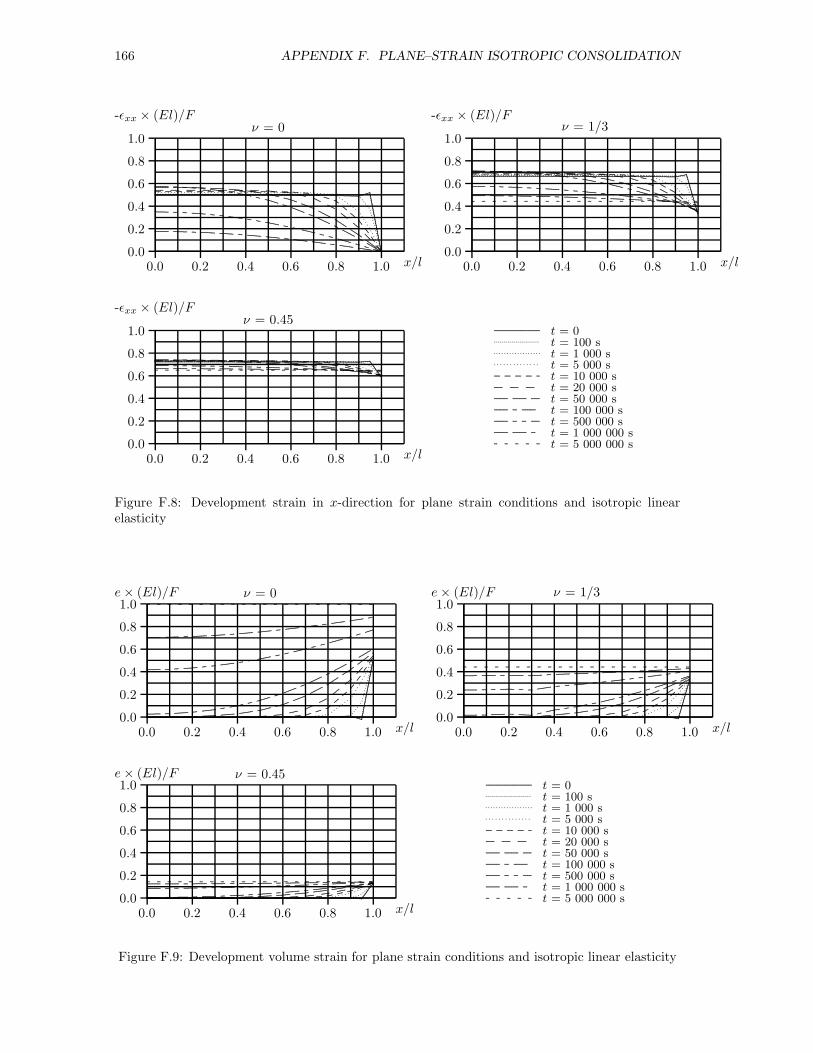
166 APPENDIX F. PLANE–STRAIN ISOTROPIC CONSOLIDATION
0.0 0.2 0.4 0.6 0.8 1.00.0
0.2
0.4
0.6
0.8
1.0
-ǫxx × (El)/Fν = 0
x/l
............................................................................................................................................................................................................................................................................................................................................................................................................................................................................................................................................
..........................................................................................................................................
.....................................................................................................
..............................................................................
........... ........... ........... ........... ........... ........... ........... ........... ........... ........... ........... ........... ........... ........... ........... ........... ........... ......................
......................
.................................
................ ................ ................ ................ ................ ................ ................ ................ ................ ................ ................................
................................
................
...............
.......................... .......................... .......................... .......................... .......................... .......................... .......................... .......................... ....................................................
....................................................
...........................
.......................... ........ .......................... ........ .......................... ........ .......................... ........ .......................... ........ .......................... ........ .......................... ..................................
..................................
.......................... ........ ........ .......................... ........ ........ .......................... ........ ........ .......................... ........ ........ .......................... ........ ........ .......................... ........ ........ ................
.......................... .......................... ........ .......................... .......................... ........ .......................... .......................... ........ .......................... .......................... ........ .......................... .......................... .............. ...... ...... ...... ...... ...... ...... ...... ...... ...... ...... ...... ...... ...... ...... ...... ...... ...... ...... ...... ...... ......
0.0 0.2 0.4 0.6 0.8 1.00.0
0.2
0.4
0.6
0.8
1.0
-ǫxx × (El)/Fν = 1/3
x/l
.......................................................................................................................................................................................................................................................................................................................................................................................................................................................................................................
................................................................................................................................
..............................................................................................
.........................................................................
........... ........... ........... ........... ........... ........... ........... ........... ........... ........... ........... ........... ........... ........... ........... ........... ........... ......................
......................
....................
................ ................ ................ ................ ................ ................ ................ ................ ................ ................ ................................
................................
................
.......................... .......................... .......................... .......................... .......................... .......................... .......................... .......................... .......................... .......................... .......................... .......................... ...................
.......................... ........ .......................... ........ .......................... ........ .......................... ........ .......................... ........ .......................... ........ .......................... ........ .......................... ........ ................
.......................... ........ ........ .......................... ........ ........ .......................... ........ ........ .......................... ........ ........ .......................... ........ ........ .......................... ........ ........ .........
.......................... .......................... ........ .......................... .......................... ........ .......................... .......................... ........ .......................... .......................... ........ .......................... .......................... .............. ...... ...... ...... ...... ...... ...... ...... ...... ...... ...... ...... ...... ...... ...... ...... ...... ...... ...... ...... ...... ......
0.0 0.2 0.4 0.6 0.8 1.00.0
0.2
0.4
0.6
0.8
1.0
-ǫxx × (El)/Fν = 0.45
x/l
..............................................................................................................................................................................................................................................................................................................................................................................................................................................................
......................................................................................
......................................................................................................................
.......................
........................................................................................
..................
......................................................................
......................... ........... ........... ........... ........... ........... ........... ........... ........... ........... ........... ........... ........... ........... ........... ........... ........... ........... ........... ........... ........... ........... ........... ........... ........... ........... ......
................ ................ ................ ................ ................ ................ ................ ................ ................ ................ ................ ................ ................ ................ ..........
................ ................ ................
.......................... .......................... .......................... .......................... .......................... .......................... .......................... .......................... .......................... .......................... .......................... .......................... .........
.......................... .......................... ................
.......................... ........ .......................... ........ .......................... ........ .......................... ........ .......................... ........ .......................... ........ .......................... ........ .......................... ........ .........
.......................... ........ ..........................
.......................... ........ ........ .......................... ........ ........ .......................... ........ ........ .......................... ........ ........ .......................... ........ ........ .......................... ........ ........ .......
.......................... ........ ........ ................
.......................... .......................... ........ .......................... .......................... ........ .......................... .......................... ........ .......................... .......................... ........ .......................... .......................... .......
.......................... .......................... ........
...... ...... ...... ...... ...... ...... ...... ...... ...... ...... ...... ...... ...... ...... ...... ...... ...... ...... ...... ...... ...... ......
...... ...... ...... ...... ......
t = 0t = 100 st = 1 000 st = 5 000 st = 10 000 st = 20 000 st = 50 000 st = 100 000 st = 500 000 st = 1 000 000 st = 5 000 000 s
Figure F.8: Development strain in x-direction for plane strain conditions and isotropic linearelasticity
0.0 0.2 0.4 0.6 0.8 1.00.0
0.2
0.4
0.6
0.8
1.0e× (El)/F ν = 0
x/l...............................................................................................................................................................................................................................................................................................................................................................................................................................
.....
.....
.....
.....
.....
.....
.....
.....
.....
.....
.....
.....
.....
.....
.....
.....
.....
.....
.....
.....
.....
....
..........................................................................................................................................
.....................................................................................................
..............................................................................
........... ........... ........... ........... ........... ........... ........... ........... ........... ........... ........... ........... ........... ........... ........... ......................
.............................................................................
................ ................ ................ ................ ................ ................ ................ ................ ................................
................
................
................................................
...............
.......................... .......................... .......................... .......................... .......................... ..............................................
...... ..........................
....................................................
..........................
.....................................................
.......................... ........ .......................... ........ .................................. ........................
.. ........ ..........................
.................................
. ..........................................
..........................
..................................
.......................... ........ ........ .......................... ........ ........ .................................. ........ .......................
... ........ ........ .......................... ........ ........
..........................
................
................
.......................... .......................... ........ .......................... .......................... ........ .......................... .......................... ........ .......................... .................................. ..........................
..................................
...... ...... ...... ...... ...... ...... ...... ...... ...... ...... ...... ...... ...... ...... ...... ...... ...... ...... ...... ...... ...... ......
0.0 0.2 0.4 0.6 0.8 1.00.0
0.2
0.4
0.6
0.8
1.0e× (El)/F ν = 1/3
x/l..............................................................................................................................................................................................................................................................................................................................................................................................................................
.....
....................................................................
................................................................................................................................
..............................................................................................
.........................................................................
........... ........... ........... ........... ........... ........... ........... ........... ........... ........... ........... ........... ........... ........... ........... ........... ........... ................................................................
................ ................ ................ ................ ................ ................ ................ ................ ................ ...............................
................
.................
................
................
.......................... .......................... .......................... .......................... .......................... .......................... .................................................
... ..........................
..........................
.......................... ............
.................................
.......................... ........ .......................... ........ .......................... ........ .......................... ........ .........................
. ........ .......................... ........
..........................
.......................
...................
.................
.......................... ........ ........ .......................... ........ ........ .................................. ........ .......................... ........ ........ .......................... ........ ........ ..........................
........ ........ .................................... .......................... ........ .......................... .......................... ........ .......................... .......................... ........ .......................... .......................... ........ .......................... .......................... .............. ...... ...... ...... ...... ...... ...... ...... ...... ...... ...... ...... ...... ...... ...... ...... ...... ...... ...... ...... ...... ......
0.0 0.2 0.4 0.6 0.8 1.00.0
0.2
0.4
0.6
0.8
1.0e× (El)/F ν = 0.45
x/l...............................................................................................................................................................................................................................................................................................................................................................................................................................
...............................
......................................................................................
......................................................................................................................
.......................
........................................................................................
..................
..............................................................
........
..............
........... ........... ........... ........... ........... ........... ........... ........... ........... ........... ........... ........... ........... ........... ........... ........... ........... ........... ........... ......................
...........
........... ........... ........... ........... ......
................ ................ ................ ................ ................ ................ ................ ................ ................ ................ ................ ................................
..........................
................ ................ ................
.......................... .......................... .......................... .......................... .......................... .......................... .......................... .......................... .......................... ....................................................
...................................
.......................... .......................... ................
.......................... ........ .......................... ........ .......................... ........ .......................... ........ .......................... ........ .......................... ........ .......................... ........ .......................... ........ .........
.......................... ........ ..........................
.......................... ........ ........ .......................... ........ ........ .......................... ........ ........ .......................... ........ ........ .......................... ........ ........ .......................... ........ ........ .......
.......................... ........ ........ ................
.......................... .......................... ........ .......................... .......................... ........ .......................... .......................... ........ .......................... .......................... ........ .......................... .......................... ................................. .......................... ........
...... ...... ...... ...... ...... ...... ...... ...... ...... ...... ...... ...... ...... ...... ...... ...... ...... ...... ...... ...... ...... ......
...... ...... ...... ...... ......
t = 0t = 100 st = 1 000 st = 5 000 st = 10 000 st = 20 000 st = 50 000 st = 100 000 st = 500 000 st = 1 000 000 st = 5 000 000 s
Figure F.9: Development volume strain for plane strain conditions and isotropic linear elasticity
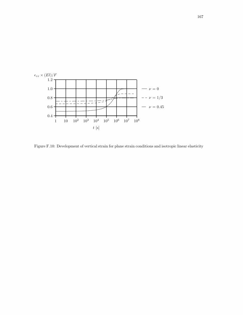
167
1 10 102 103 104 105 106 107 108
t [s]
0.4
0.6
0.8
1.0
1.2ǫzz × (El)/F
........................................................................................................................................................................................................................................................................
.......................................
........................................................................................................................................................................................................................................................................ .................................
............. ............. ............. ............. ............. ............. ............. ............. ............. ............. ............. ............. ............. ..........................
.......................................
.......................... ............. ............. ...........
............. ..........
.......................... ........ .......................... ........ .......................... ........ .......................... ........ .......................... ........ .......................... ........ .................................. ..........................
........ .......................... ........ ......................
..........................
ν = 0
ν = 1/3
ν = 0.45
Figure F.10: Development of vertical strain for plane strain conditions and isotropic linear elasticity

168 APPENDIX F. PLANE–STRAIN ISOTROPIC CONSOLIDATION

Appendix G
Consolidation for cross–anisotropic
axial–symmetric conditions
In this appendix the solution for isotropic linear elasticity presented in appendix E is extendedfor cross–anisotropy. Again the solution is derived in 4 steps:
step 1, the relevant expressionsBasic equations for axial symmetry:
∇2 =∂2
∂r2+
1
r
∂
∂r+
1
r2∂2
∂θ2+
∂2
∂z2
εr =∂ur∂r
, εθ =urr
+1
r
∂uθ∂θ
, εzz =∂uzz∂z
γθz =∂uθ∂z
+∂uzzr∂θ
, γrz =∂ur∂z
+∂uzz∂r
, γrθ =∂urr∂θ
+∂uθ∂r
− uθr
Simplifications due to axial symmetry and the stiff plate on top:
axial symmetry:∂
∂θ= 0
stiff plate on top:∂εzz∂z
=∂εzz∂r
= 0
no shear stresses and strains: γθz = γrθ = γrz = τθz = τrθ = τrz = 0
So strain is expressed into:
εr =∂ur∂r
εθ =urr
εz =∂uzz∂z
e =∂ur∂r
+urr
+∂uzz∂z
=1
r
∂ (r ur)
∂r+∂uzz∂z
(G.1)
The stress–strain relationship is elaborated given in appendix B:
σ′
r = Ae+ 2Ghh εr +Bεzz
σ′
θ = Ae+ 2Ghh εθ +Bεzz (G.2)
σ′
zz = (A+B) e+Dεzz
169
170 APPENDIX G. AXIAL–SYMMETRICAL ANISOTROPIC CONSOLIDATION
Appendix H elaborates the equilibrium of forces for cross–anisotropic conditions in cartesianco-ordinates. For cylindrical co–ordinates the equilibrium condition is found in an equivalent way:
[A+ 2Ghh]∇2e = ∇2σw (G.3)
The storage equation remains unaffected:
k
γw∇2σw =
∂e
∂t(G.4)
Combination of equation (G.3) and (G.4) gives:
k
γw[A+ 2Ghh]∇2e =
∂e
∂t(G.5)
with c = k [A+ 2Ghh] /γw:
∇2e =1
c
∂e
∂t(G.6)
step 2, the Laplace transformationSolving equation (G.6) with Laplace transformation:
∇2e =1
c[se− e0] , e0 = 0
∇2e =s
ce, → ∂2e
∂r2+
1
r
∂e
∂r− s
ce = 0
standard solution:
e = C1J0 (λr) + C2Y0 (λr) , λ =
√−sc
(G.7)
Application of the Laplace transform to equation (G.3):
[A+ 2Ghh]∇2e = ∇2σw
∇2e =∇2σw
A+ 2Ghh
e =1
A+ 2Ghhσw + C3, ∇2C3 = 0 (G.8)
e =1
r
∂ (rur)
∂r+∂uzz∂z
σw = [A+ 2Ghh] [e− C3]
σw = [A+ 2Ghh] [C1J0 (λr) + C2Y0 (λr) − C3] (G.9)
1
r
∂ (rur)
∂r= C1J0 (λr) + C2Y0 (λr) − ∂uzz
∂z(G.10)
Integration of equation (G.10) gives:
urR
= C1J1 (λr)
λR+ C2
Y1 (λr)
λR− r
2R
∂uzz∂z
+C4
rR(G.11)
Differentiation of equation (G.11) results in:
∂ur∂r
= C1
[J0 (λr) − J1 (λr)
λr
]+ C2
[Y0 (λr) − Y1 (λr)
λr
]− 1
2
∂uzz∂z
− C4
r2(G.12)
Using equation (G.2) stress and strain are expressed into:
e = C1J0 (λr) + C2Y0 (λr) (G.13)

171
σw = [A+ 2Ghh] [C1J0 (λr) + C2Y0 (λr) − C3] (G.14)
σ′
r = A [C1J0 (λr) + C2Y0 (λr)] + 2Ghh
C1
[J0 (λr) − J1 (λr)
λr
]
+C2
[Y0 (λr) − Y1 (λr)
λr
]− 1
2
∂uzz∂z
− C4
r2
+B∂uzz∂z
(G.15)
σ′
θ = A [C1J0 (λr) + C2Y0 (λr)] + 2Ghh
[C1J1 (λr)
λr+ C2
Y1 (λr)
λr
]+ (G.16)
2Ghh
[−1
2
∂uzz∂z
+C4
r2
]+B
∂uzz∂z
σ′
z = (A+B) [C1J0 (λr) + C2Y0 (λr)] +D∂uzz∂z
(G.17)
σr = σ′
r − σw (G.18)
σθ = σ′
θ − σw (G.19)
σzz = σ′
zz − σw (G.20)
step 3, solving for boundary conditionsIn the equations (G.13) to (G.20) 5 unknown parameters remain; C1, C2, C3, C4 and ∂uzz/∂z.Since e in equation (G.13) and σ′
r in equation (G.15) have a limited value when r reaches 0, itfollows that C2 = C4 = 0. The remaining unknown parameters can be solved by the boundaryconditions:
a) at r = R σw = g1, → σw = g1
b) at r = R σr = g2, → σr = g2
c) at z = h 1/A∫
2πrσzzdr = g3, → 1/A∫
2πrσzzdr = g3
The combination of boundary condition a and equation (G.14) gives:
C3 = C1J0 (λR) − g1
A+ 2Ghh(G.21)
rewriting equation (G.18) gives:
σr = AC1J0 (λr) + 2Ghh
[C1J0 (λr) − C1
J1 (λr)
λr
]+ (B −Ghh)
∂uzz∂z
− [A+ 2Ghh] [C1J0 (λr) − C1J0 (λR)] − g1
σr = −2GhhC1J1 (λr)
λr+ [B −Ghh]
∂uzz∂z
+ [A+ 2Ghh]C1J0 (λR) − g1
The application of boundary condition b to equation (G.18) gives:
g2 = −2GhhC1J1 (λR)
λR+ [B −Ghh]
∂uzz∂z
+ [A+ 2Ghh]C1J0 (λR) − g1
∂uzz∂z
=C1
B −Ghh
[2Ghh
J1 (λR)
λR− (A+ 2Ghh)J0 (λR)
]+
g1 + g2
B −Ghh(G.22)
Application of boundary condition c to equation (G.20) gives:
σzz = C1 (A+B)J0 (λr) +D∂uzz∂z
− (A+ 2Ghh)
[C1 (J0 (λr) − J0 (λR)) +
g1
A+ 2Ghh
]
σzz = C1
[(B − 2Ghh)J0 (λr) +
[1 − D
B −Ghh
](A+ 2Ghh)J0 (λR)
]− g1
+D (g1 + g2)
B −Ghh+DC12GhhB −Ghh
J1 (λR)
λR
(G.23)

172 APPENDIX G. AXIAL–SYMMETRICAL ANISOTROPIC CONSOLIDATION
with:
g3 =
R∫
0
2πr
πR2σzzdr
follows:
g3 =
R∫
0
2r
R2
(B − 2Ghh)C1J0 (λr) + (A+ 2Ghh)C1J0 (λR)
[1 − D
B −Ghh
]
−g1 +C12GhhD
B −Ghh
J1 (λR)
λR+D (g1 + g2)
B −Ghh
dr
g3 = 2 (B − 2Ghh)C1J1 (λR)
λR+ C1 (A+ 2Ghh)J0 (λR)
[1 − D
B −Ghh
]+
2DGhhB −Ghh
C1J1 (λR)
λR− g1 +
D (g1 + g2)
B −Ghh
C1 =g3 + g1 −
D (g1 + g2)
B −Ghh
2J1 (λR)
λR
[B − 2Ghh +
DGhhB −Ghh
]+ (A+ 2Ghh)J0 (λR)
[1 − D
B −Ghh
] (G.24)
Equation (G.22) and (G.24) give:
∂uzz∂z
=
(g3 + g1 −
D (g1 + g2)
B −Ghh
)[2G
B −Ghh
J1 (λR)
λR− A+ 2Ghh
B −GhhJ0 (λR)
]
2J1 (λR)
λR
[(B − 2Ghh) +
DGhhB −Ghh
]+ J0 (λR) (A+ 2Ghh)
[1 − D
B −Ghh
]
+g1 + g2
B −Ghh
(G.25)
step 4, inverse transformationThe inverse transformation starts with finding an expression for the boundary conditions g1, g2
and g3. Standard triaxial testing with a radial pore pressure flow is modelled by g1 = g2 = 0,g3 = σb. The boundary conditions in transformed conditions is then given by:
g1 = 0
g2 = 0
g3 =
∞∫
0
σb exp (−st) dt =σbs
The expression for σw is then given by:
σwσb
=J0 (λr) − J0 (λR)
s
[2J1 (λR)
[A+ 2Ghh]λR
[(B − 2Ghh) +
DGhhB −Ghh
]+ J0 (λR)
(1 − D
B −Ghh
)] (G.26)
Equivalent to appendix E the Heaviside expansion theorem is used for finding the inversetransform of equation (G.26). A removable root is found for s = 0, the other roots are found forvalues of defined by:
2J1 (λR)
[A+ 2Ghh]λR
[B − 2Ghh +
GhhD
B −Ghh
]= J0 (λR)
[D
B −Ghh− 1
]
J1 (λR)
J0 (λR)= CλR, C =
1
2
A+ 2Ghh
B − 2Ghh +DGhhB −Ghh
[D
B −Ghh− 1
](G.27)
173
The values for s that fulfil condition (G.27) are indicated by sj . The expression for σw is nowgiven by:
σwσb
=
∞∑
j=1
[J0 (λjr) − J0 (λjR)] esjt
sj∂
∂s
[2J1 (λjR)
(A+ 2Ghh) λjR
[B − 2Ghh +
GhhD
B −Ghh
]+ J0 (λjR)
(1 − D
B −Ghh
)]
Elaborating the differentiation of the denominator
∂
∂s
(J1 (λjR)
λjR
)= −2J1 (λjR)
2λjRsj+
1
2sjJ0 (λjR)
∂
∂s(J0 (λjR)) = −J1 (λjR)λjR
2sj
∂
∂s
[2J1 (λjR)
(A+ 2Ghh)λjR
[B − 2Ghh +
GhhD
B −Ghh
]+ J0 (λjR)
(1 − D
B −Ghh
)]=
2
A+ 2Ghh
[−J1 (λjR)
λjRsj+
1
2sjJ0 (λjR)
] [(B − 2Ghh) +
GhhD
B −Ghh
]
−J1 (λjR)
2sj(λjR)
(1 − D
B −Ghh
)=
1
s
[− 2J1 (λjR)
(A+ 2Ghh)λjR+
J0 (λjR)
A+ 2Ghh
] [(B − 2Ghh) +
GhhD
B −Ghh
]+
1
s
[1
2J1 (λjR)
(D
B −Ghh− 1
)λjR
]
Combination with equation (G.27) gives:
1
s
[J0 (λjR)
A+ 2Ghh
[B − 2Ghh +
GhhD
B −Ghh
]+
[λjRJ1 (λjR)
2− J0 (λjR)
] [D
B −Ghh− 1
]]
Adding this result to equation (G.26) gives:
σwσb
=
∞∑
j=1
[J0 (λjr) − J0 (λjR)] esjt
s1
s
[J0 (λjR)
A+ 2Ghh
[B − 2Ghh +
DGhhB −Ghh
]+
[λjR
2J1 (λjR) − J0 (λjR)
] [D
B −Ghh− 1
]]
(G.28)rewriting gives:
σwσb
=
∞∑
j=1
[J0 (λjr)
J0 (λjR)− 1
]esjt
[B − 2Ghh +DGhh/ (B −Ghh)
A+ 2Ghh
]+
[λjR
2
J1 (λjR)
J0 (λjR)− 1
] [D
B −Ghh− 1
] (G.29)
Function f(t)
Section 5.2 explains that the difference between the Biot equations and the Terzaghi–Rendulicsolution for three dimensional consolidation is found in equation (G.3). Twice integratingequation (G.3) gives:
[A+ 2Ghh] e = σw + f (x, y, z, t) (G.30)
In the Terzaghi–Rendulic solution a direct relation between e and σw is assumed, leading tof(x, y, z, t) = 0. De Josselin de Jong [41] shows that in absence of rotations f(x, y, z, t) reduces tof(t) but not necessarily to 0. With the solutions found for e and σw an expression for f(t) can befound. The Laplace transformation of equation (G.30) gives:
[A+ 2Ghh] e = σw + f(t) (G.31)

174 APPENDIX G. AXIAL–SYMMETRICAL ANISOTROPIC CONSOLIDATION
With the equations (G.7) and (G.9) it is found that:
f(t) = C3 (A+ 2Ghh) (G.32)
With C3 expressed by equation (G.21) it is found after rewriting that:
f(t) =
J0 (λR)
(g3 −
D (g2 + g1)
B −Ghh
)− g1
[2J1 (λR)
λR (A+ 2Ghh)
(B − 2Ghh +
DGhhB −Ghh
)+DJ0 (λR)
B −Ghh
]
2J1 (λR)
λR (A+ 2Ghh)
[B − 2Ghh +
DGhhB −Ghh
]+B −Ghh −D
B −GhhJ0 (λR)
(G.33)The inverse transformation is found equivalent to the previous given inverse transforms of stressand strain. With condition (E.37) it is found for g1 = g2 = 0 and g3 = σb that:
f(t) =(A+ 2Ghh) (B −Ghh)σb
(B −Ghh)B +A (B −Ghh −D) −GhhD+
∞∑
j=1
σbesjt
[B − 2Ghh +DGhh/ (B −Ghh)
A+ 2Ghh
]+
[λjR
2
J1 (λjR)
J0 (λjR)− 1
] [D
B −Ghh− 1
](G.34)
Non–perfect drainage
Due to hydraulic resistance in the drains, porous stone and the pore water collection systemboundary condition a might not hold in practice. To study the influence of non–perfect drainagesystem a time depending boundary condition can be used. Section 5.5 suggest the followingboundary condition:
g1 = −1
3σbe
−κt
In which the parameters κ controls the drain pressure decay. The complete set of boundaryconditions becomes:
g1 = −[1
3+K ′
J ′
]σbe
−κt, → g1 = −[1
3+K ′
J ′
]σbκ+ s
g2 = 0 → g2 = 0
g3 = σb → g3 =σbs
Application of this set of boundary conditions to equation (G.13) gives:
σw =[J0 (λr) − J0 (λR)]σb
s
[2J1 (λR)
(A+ 2Ghh)λR
(B − 2Ghh +
DGhhB −Ghh
)+B −Ghh −D
B −GhhJ0 (λR)
]−
[J0 (λr) − J0 (λR)]
(1
3+K ′
J ′
)B −Ghh −D
B −Ghhσb
(κ+ s)
[2J1 (λR)
(A+ 2Ghh)λR
(B − 2Ghh +
DGhhB −Ghh
)+B −Ghh −D
B −GhhJ0 (λR)
]
−(
1
3+K ′
J ′
)σbκ+ s
(G.35)
The right hand side of equation (G.35) consists of three parts. In application of the inversetransformation each part can be transformed individually. The inverse transform of the first parthas already been given by equation (G.29). The third part follows directly from boundaryconditions or can be found in handbooks for standard solution:
L−1
(1
3+K ′
J ′
)σbκ+ s
=
(1
3+K ′
J ′
)σbe
−κt
175
For finding the inverse transform of the second part the Heaviside expansion theorem is used.The roots of the second term are given by:
s = −κ ∨ 2J1 (λR)
(A+ 2Ghh)λR
(B − 2Ghh +
GhhD
B −Ghh
)+B −Ghh −D
B −GhhJ0 (λR) = 0
The second group of roots equal the roots given by equation (G.27). The derivative of thedenominator of the second term in equation (G.35) is given by:
[2J1 (λR)
(A+ 2Ghh)λR
(B − 2Ghh +
GhhD
B −Ghh
)+B −Ghh −D
B −GhhJ0 (λR)
]+
κ+ s
s
[J0 (λR)
A+ 2Ghh
(B − 2Ghh +
DGhhB −Ghh
)+
[λR
2J1 (λR) − J0 (λR)
] [D
B −Ghh− 1
]]
Summation of the three parts gives the inverse transform of equation (G.35):
σwσb
=
∞∑
j=1
[J0 (λjr)
J0 (λjR)− 1
]esjt
[B − 2Ghh +DGhh/ (B −Ghh)
A+ 2Ghh
]+
[λjR
2
J1 (λjR)
J0 (λjR)− 1
]+
[D
B −Ghh− 1
]−
∞∑
j=1
[J0 (λjr)
J0 (λjR)− 1
](1
3+K ′
J ′
)B −Ghh −D
B −Ghhesjt
κ+ sjsj
[B − 2Ghh +DGhh/ (B −Ghh)
A+ 2Ghh
]+
[λjR
2
J1 (λjR)
J0 (λjR)− 1
]+
[D
B −Ghh− 1
]−
[J0
(√κ
cr
)/J0
(√κ
cR
)− 1
](1
3+K ′
J ′
)B −Ghh −D
B −Ghhe−κt
2J1
(√κ
cR
)(B − 2Ghh +
DGhhB −Ghh
)
(A+ 2Ghh)J0
(√κ
cR
)√κ
cR
+B −Ghh −D
B −Ghh
−(
1
3+K ′
J ′
)e−κt
(G.36)
Isotropic loading
Using equations (G.9), (G.21) and (G.24) the pore pressure development for isotropic loadinginstead of axial loading is easily found. For the boundary conditions g1 = 0 and g2 = g3 = σbfollows:
σwσb
=
B −Ghh −D
B −GhhJ0 (λr) − J0 (λR)
s
[2J1 (λR)
[A+ 2Ghh]λR
[(B − 2Ghh) +
DGhhB −Ghh
]+ J0 (λR)
(1 − D
B −Ghh
)] (G.37)
Equation (G.37) differs only from equation (G.26) by the constant (B −Ghh −D)/(B −Ghh).The inverse transform gives:
σwσb
=
∞∑
j=1
B −Ghh −D
B −Ghh
[J0 (λjr)
J0 (λjR)− 1
]esjt
[B − 2Ghh +DGhh/ (B −Ghh)
A+ 2Ghh
]+
[λjR
2
J1 (λjR)
J0 (λjR)− 1
]+
[D
B −Ghh− 1
] (G.38)
Note that the reciprocal value for the constant (B −Ghh −D)/(B −Ghh) can be rewritten, usingthe expressions given in the appendix B, into:
B −GhhB −Ghh −D
= −(
1
3+K ′
J ′
)

176 APPENDIX G. AXIAL–SYMMETRICAL ANISOTROPIC CONSOLIDATION
Consolidation around a vertical drain
Based on the solution for consolidation of a triaxial sample the solution for consolidation arounda vertical drain can be solved. This solution is found when solving equation (G.11) to (G.20) for adifferent set of boundary conditions. With ρ the radius of the drain and R the outer radius of thecylinder in which the drain is active, the following five boundary conditions describe the problem;
a) at r = ρ σw = 0, → σw = 0
b) at r = R ur = 0, → ur = 0
c) at r = ρ ur = 0, → ur = 0
d) at r = R ∂σw/∂r = 0, → ∂σw/∂r = 0
e) at z = h 1/A∫
2πrσzzdr = σb, → 1/A∫
2πrσzzdr = σb
The combination of boundary condition a and equation (G.14) gives:
C3 = C1J0 (λρ) + C2Y0 (λρ) (G.39)
The combination of boundary condition b and equation (G.11) gives:
1
2
∂uzz∂z
= C1J1 (λR)
λR+ C2
Y1 (λR)
λR+C4
R2(G.40)
The combination of boundary condition c and equation (G.11) gives:
C4 = ρR
[ρ
2R
∂uzz∂z
− C1J1 (λρ)
λR− C2
Y1 (λρ)
λR
](G.41)
Application of equation (G.40) gives:
C4 =ρR2
R2 − ρ2
[C1
(ρJ1 (λR)
λR−R
J1 (λρ)
λR
)+ C2
(ρY1 (λR)
λR−R
Y1 (λρ)
λR
)](G.42)
The derivative of equation (G.14) gives, with C3 independent of r:
∂σw∂r
= − (A+ 2Ghh) [C1λJ1 (λr) + C2λY1 (λr)]
with boundary condition d follows:
C1 = −C2Y1 (λR)
J1 (λR)(G.43)
Finally with boundary condition e and equation (G.17) and (G.20) :
σb =
R∫
ρ
2πr
π (R2 − ρ2)σzzdr
σzz = (B − 2Ghh) [C1J0 (λr) + C2Y0 (λr)] +D∂uzz∂z
+ (A+ 2Ghh)C3
σb = (B − 2Ghh)
C1
(2R2
R2 − ρ2
J1 (λR)
λR− 2ρ2
R2 − ρ2
J1 (λρ)
λρ
)+
C2
(2R2
R2 − ρ2
Y1 (λR)
λR− 2ρ2
R2 − ρ2
Y1 (λρ)
λρ
)
+D∂uzz∂z
+ (A+ 2Ghh)C3
Application of equation (G.39), (G.40), (G.42) and (G.43) gives:
C2 =J1 (λR)σb
α
λR(Y1 (λρ)J1 (λR) − J1 (λρ) Y1 (λR))+
(A+ 2Ghh) [Y0 (λρ)J1 (λR) − Y1 (λR)J0 (λρ)]
(G.44)

177
and:
C1 =−Y1 (λR) σb
α
λR(Y1 (λρ)J1 (λR) − J1 (λρ) Y1 (λR))+
(A+ 2Ghh) [Y0 (λρ)J1 (λR) − Y1 (λR)J0 (λρ)]
(G.45)
with:
α = (2Ghh −B −D)2ρR
(R2 − ρ2)(G.46)
With expressions available for C1, C2, C3, C4 and ∂uzz/∂z an expression for each stress andstrain can be found. This is elaborated for εzz, ur, εr, e, σw and σ′
r. From equations (G.40),(G.11), (G.12), (G.13), (G.14) and (G.15) is found in transformed conditions:
εzz =∂uzz∂z
=2ρR
R2 − ρ2
Y1 (λR)J1 (λρ)
λR− J1 (λR)
Y1 (λρ)
λR
α
λR(Y1 (λρ) J1 (λR) − J1 (λρ)Y1 (λR))+
(A+ 2Ghh) [Y0 (λρ) J1 (λR) − Y1 (λR)J0 (λρ)]
× σb (G.47)
urR
=
−Y1 (λR)
[J1 (λr)
λR−ρ(R2 − r2
)
r (R2 − ρ2)
J1 (λρ)
λR
]+
J1 (λR)
[Y1 (λr)
λR−ρ(R2 − r2
)
r (R2 − ρ2)
Y1 (λρ)
λR
]
α
λR(Y1 (λρ) J1 (λR) − J1 (λρ) Y1 (λR))+
(A+ 2Ghh) [Y0 (λρ)J1 (λR) − Y1 (λR)J0 (λρ)]
× σb (G.48)
εr =
J1 (λR)
[Y0 (λr) − Y1 (λr)
λr+R
ρ(r2 +R2
)
r2 (R2 − ρ2)
Y1 (λρ)
λR
]−
Y1 (λR)
[J0 (λr) − J1 (λr)
λr+R
ρ(r2 +R2
)
r2 (R2 − ρ2)
J1 (λρ)
λR
]
α
λR(Y1 (λρ)J1 (λR) − J1 (λρ)Y1 (λR)) +
(A+ 2Ghh) [Y0 (λρ)J1 (λR) − Y1 (λR)J0 (λρ)]
× σb (G.49)
e =J1 (λR)Y0 (λr) − Y1 (λR)J0 (λr)
α
λR(Y1 (λρ) J1 (λR) − J1 (λρ)Y1 (λR))+
(A+ 2Ghh) [Y0 (λρ) J1 (λR) − Y1 (λR) J0 (λρ)]
× σb (G.50)
σw =(A+ 2Ghh) (−Y1 (λR) (J0 (λr) − J0 (λρ)) + J1 (λR) (Y0 (λr) − Y0 (λρ)))σb
α
λR(Y1 (λρ)J1 (λR) − J1 (λρ)Y1 (λR)) +
(A+ 2Ghh) [Y0 (λρ)J1 (λR) − Y1 (λR)J0 (λρ)]
(G.51)
σ′
r =
−Y1 (λR)
[(A+ 2Ghh)J0 (λr) − 2Ghh
J1 (λr)
λr− ξ (r)
J1 (λρ)
λR
]+
J1 (λR)
[(A+ 2Ghh)Y0 (λr) − 2Ghh
Y1 (λr)
λr− ξ (r)
Y1 (λρ)
λR
]
α
λR(Y1 (λρ) J1 (λR) − J1 (λρ) Y1 (λR))+
(A+ 2Ghh) [Y0 (λρ)J1 (λR) − Y1 (λR) J0 (λρ)]
× σb (G.52)
with:
ξ (r) =
(2 (B −Ghh)
R2− 2Ghh
r2
)ρR3
R2 − ρ2

178 APPENDIX G. AXIAL–SYMMETRICAL ANISOTROPIC CONSOLIDATION
The inverse of equations (G.47) to (G.52) can be found using the Heaviside expansion theorem.The Heaviside expansion theorem starts with finding the roots of the denominator. The roots ofthe denominator are given by the values for s that fulfil:
s = 0 ∨ Y1 (λρ) J1 (λR) − J1 (λρ) Y1 (λR)
Y0 (λρ) J1 (λR) − Y1 (λR)J0 (λρ)= − (A+ 2Ghh)
αλR (G.53)
Next the derivative of the denominator is needed. When d represents the denominator thefollowing is found:
∂d
∂s=
α
λR(Y1 (λρ) J1 (λR) − J1 (λρ) Y1 (λR))+
(A+ 2Ghh) [Y0 (λρ)J1 (λR) − Y1 (λR)J0 (λρ)]
× ∂
∂s(s)+
s× ∂
∂s
α
λR(Y1 (λρ) J1 (λR) − J1 (λρ) Y1 (λR))+
(A+ 2Ghh) [Y0 (λρ)J1 (λR) − Y1 (λR)J0 (λρ)]
Application of condition (G.53) gives for s 6= 0:
∂d
∂s= αψ + (A+ 2Ghh)φ
with:
ψ = Y1 (λρ)
[1
2J0 (λR) − J1 (λR)
λR
]+J1 (λR)
λR
[λρ
2Y0 (λρ) − 1
2Y1 (λρ)
]−
J1 (λρ)
[1
2Y0 (λR) − Y1 (λR)
λR
]− Y1 (λR)
λR
[λρ
2J0 (λρ) − 1
2J1 (λρ)
]
φ =1
2[λRJ0 (λR) Y0 (λρ) − λRJ0 (λρ)Y0 (λR) − λρY1 (λρ)J1 (λR)]
+1
2[λρY1 (λR)J1 (λρ) − J1 (λR)Y0 (λρ) + J0 (λρ)Y1 (λR)]
gives:
εzzσb
=1
σb
∂uzz∂z
=1
A+B +D+
2ρR
R2 − ρ2
∞∑
j=1
Y1 (λjR)J1 (λjρ)
λjR− J1 (λjR)
Y1 (λjρ)
λjR
αψj + (A+ 2Ghh)φj× esjt (G.54)
1
σb
urR
=
∞∑
j=1
J1 (λjR)
[Y1 (λjr)
λjR−ρ(R2 − r2
)
r (R2 − ρ2)
Y1 (λjρ)
λjR
]−
Y1 (λjR)
[J1 (λjr)
λjR−ρ(R2 − r2
)
r (R2 − ρ2)
J1 (λjρ)
λjR
]
αψj + (A+ 2Ghh)φj× esjt
(G.55)
εrσb
=
∞∑
j=1
J1 (λjR)
[Y0 (λjr) −
Y1 (λjr)
λjr
]− Y1 (λjR)
[J0 (λjr) −
J1 (λjr)
λjr
]+
Rρ(r2 +R2
)
r2 (R2 − ρ2)
[J1 (λjR)Y1 (λjρ)
λjR− Y1 (λjR)J1 (λjρ)
λjR
]
αψj + (A+ 2Ghh)φj× esjt
(G.56)
e
σb=
1
A+B +D+
∞∑
j=1
J1 (λjR)Y0 (λjr) − Y1 (λjR)J0 (λjr)
αψj + (A+ 2Ghh)φj× esjt (G.57)
σwσb
=∞∑
j=1
(A+ 2Ghh)
[J1 (λjR) (Y0 (λjr) − Y0 (λjρ))
−Y1 (λjR) (J0 (λjr) − J0 (λjρ))
]
αψj + (A+ 2Ghh)φj× esjt (G.58)
179
σrσb
=EhEv
νvh1 − νhh
+
∞∑
j=1
J1 (λjR)
[(A+ 2Ghh)Y0 (λjr) − 2Ghh
Y1 (λjr)
λjr− ξ (r)
Y1 (λjρ)
λjR
]
−Y1 (λjR)
[(A+ 2Ghh)J0 (λjr) − 2Ghh
J1 (λjr)
λjr− ξ (r)
J1 (λjρ)
λjR
]
αψj + (A+ 2Ghh)φj× esjt
(G.59)
with:
ξ (r) =
(2 (B −Ghh)
R2− 2Ghh
r2
)ρR3
R2 − ρ2
In accordance to equation (G.30) the following is found for function f(t):
f(t) = (A+ 2Ghh)C3 = (A+ 2Ghh) [C1J0 (λρ) + C2Y0 (λρ)]
Application of equations (G.44) and (G.45) gives after inverse transformation:
f(t) =A+ 2GhhA+B +D
+∞∑
j=1
(A+ 2Ghh) [J1 (λjR)Y0 (λjρ) − Y1 (λjR)J0 (λjρ)]σbesjt
αψj + (A+ 2Ghh)φj(G.60)
It should be noted that for isotropic conditions α = 0 and therefore f(t) = σb leading to f(t) =σb. With equation (G.58) the average degree of consolidation U is given by:
U =
R∫
ρ
2πr
π (R2 − ρ2)
σwσb
dr (G.61)
Elaborating equation (G.61) gives:
U =2 (A+ 2Ghh)
R2 − ρ2×
∞∑
j=1
J1 (λjR)
[R
λjY1 (λjR) − ρ
λjY1 (λjρ) −
1
2
(R2 − ρ2
)Y0 (λjρ)
]−
Y1 (λjR)
[R
λjJ1 (λjR) − ρ
λjJ1 (λjρ) −
1
2
(R2 − ρ2
)J0 (λjρ)
]
αψj + (A+ 2Ghh)φj× esjt
(G.62)

180 APPENDIX G. AXIAL–SYMMETRICAL ANISOTROPIC CONSOLIDATION
Appendix H
Consolidation for anisotropic
plane–strain conditions
This appendix extends the solution derived in appendix F to cross–anisotropic conditions. Againthe solution derived in 4 steps
step 1, the relevant equationsTo derive the solution for plane strain, cross–anisotropic conditions the stress–strain relationshipelaborated in appendix B is used:
σ′
xx = Ae+ 2Ghhεxx +Bεzz
σ′
yy = Ae+ 2Ghhεyy +Bεzz
σ′
zz = (A+B)e+Dεzz
τyz = Gvh
[∂uyy∂z
+∂uzz∂y
]
τzx = Gvh
[∂uxx∂z
+∂uzz∂x
]
τxy = Ghh
[∂uxx∂y
+∂uyy∂x
]
(H.1)
Note the sign convention in which stress is chosen positive for tension while the pore pressure ischosen positive for pressure. The effective stress is then defined by:
σ′
xx = σxx + σw
σ′
yy = σyy + σw
σ′
zz = σzz + σw
(H.2)
Equilibrium yields:
∂σ′xx
∂x+∂τxy∂y
+∂τxz∂z
=∂σw∂x
∂τyx∂x
+∂σ′
yy
∂y+∂τyz∂z
=∂σw∂y
∂τzx∂x
+∂τzy∂y
+∂σ′
zz
∂z=∂σw∂z
(H.3)
181

182 APPENDIX H. PLANE–STRAIN ANISOTROPIC CONSOLIDATION
Combination of (H.1) and (H.3) leads to:
A∂e
∂x+ 2Ghh
∂2uxx∂x2
+B∂2uzz∂x∂z
+Ghh∂2uxx∂y2
+Ghh∂2uyy∂y∂x
+Gvh∂2uxx∂z2
+Gvh∂2uzz∂z∂x
=∂σw∂x
Ghh∂2uxx∂x∂y
+Ghh∂2uyy∂x2
+A∂e
∂y+ 2Ghh
∂2uyy∂y2
+B∂2uzz∂y∂z
+Gvh∂2uyy∂z2
+Gvh∂2uzz∂z∂y
=∂σw∂y
Gvh∂2uxx∂x∂z
+Gvh∂2uzz∂x2
+Gvh∂2uyy∂y∂z
+Gvh∂2uzz∂y2
+ (A+B)∂e
∂z+D
∂2uzz∂z2
=∂σw∂z
(H.4)To simplify (H.4) the following assumptions are made:
- plane strain conditions result in: εyy = 0
- stiff top on top ∂εzz/∂z = ∂εzz/∂x = 0
- no shear stress τzx = τyx = τzy = 0
Application of these assumptions to equation (H.4) gives:
A∂e
∂x+ 2Ghh
∂2uxx∂x2
=∂σw∂x
A∂e
∂y=
∂σw∂y
A∂e
∂z+ B
∂e
∂z=
∂σw∂z
(H.5)
Differentiation and summation changes equation (H.5) into:
A∇2e+ 2Ghh∂3uxx∂x3
+B∂2e
∂z2= ∇2σw (H.6)
Note that the volumetric strain can be rewritten into:
∇2e =∂2εxx∂x2
+∂2εyy∂y2
+∂2εzz∂z2
,∂2εyy∂y2
=∂2εzz∂z2
= 0, ∇2e =∂2εxx∂x2
=∂3uxx∂x3
∂2e
∂z2=∂2εxx∂z2
+∂2εyy∂z2
+∂2εzz∂z2
,∂2εyy∂z2
=∂2εzz∂z2
= 0,
εxx is constant at every z - level,∂2εxx∂z2
= 0,∂2e
∂z2= 0
Equation (H.6) can be rewritten into:
[A+ 2Ghh]∇2e = ∇2σw (H.7)
The storage equation remains unaltered:
k
γw∇2σw =
∂e
∂t(H.8)
Combination of equation (H.7) and (H.8) gives the consolidation equation:
k
γw[A+ 2Ghh]∇2e =
∂e
∂t
or
∂2e
∂x2=
1
c
∂e
∂t, with c =
k
γw[A+ 2Ghh]
(H.9)

183
step 2, the Laplace transformationThe solution of equation (H.9) can be found by using the Laplace transformation. Application ofthe Laplace transformation to the equation (H.9) gives:
∂2e
∂x2=
1
c(se− e0) (H.10)
In which e0 is the volumetric strain directly after loading, at t = 0+. Since directly after loadingthe soil behaves undrained; e0 = 0. Equation (H.10) reduces to:
∂2e
∂x2− s
ce = 0 (H.11)
Equation (H.11) is a linear ordinary second–order differential equation and can be solved by thestandard solution : e = exp(λx):
λ2 exp(λx) − s
cexp(λx) = 0;
λ = ±√s
cand e = C1 exp
(√s
cx
)+ C2 exp
(−√s
cx
)
reformulation gives:
e = C1 cosh
(√s
cx
)+ C2 sinh
(√s
cx
)(H.12)
with (H.12):
e = εxx + εzz, e =∂uxx∂x
+∂uzz∂z
is found in combination to equation (H.12):
∂uxx∂x
= C1 cosh
(√s
cx
)+ C2 sinh
(√s
cx
)− ∂uzz
∂z(H.13)
The transform of equation (H.7):
∇2e =∇2σw
[A+ 2Ghh]
leads to:
e =σw
[A+ 2Ghh]+ C3, with ∇2C3 = 0
σw = [A+ 2Ghh]
[C1 cosh
(√s
cx
)+ C2 sinh
(√s
cx
)− C3
](H.14)
The combination of (H.1), (H.12) and (H.13) gives the expressions for stress and strain intransformed conditions:
e = C1 cosh
(√s
cx
)+ C2 sinh
(√s
cx
)(H.15)
∂uxx∂x
= C1 cosh
(√s
cx
)+ C2 sinh
(√s
cx
)− ∂uzz
∂z(H.16)
σw = [A+ 2Ghh]
[C1 cosh
(√s
cx
)+ C2 sinh
(√s
cx
)− C3
](H.17)
σ′
xx = Ae+ 2Ghh∂uxx∂x
+B∂uzz∂z
(H.18)
σ′
yy = Ae+B∂uzz∂z
(H.19)
σ′
zz = Ae+Be+D∂uzz∂z
(H.20)

184 APPENDIX H. PLANE–STRAIN ANISOTROPIC CONSOLIDATION
σxx = σxx − σw
σyy = σyy − σw
σzz = σzz − σw
(H.21)
step 3, solving for the boundary conditionsThe equations (H.15) to (H.21) contain 4 unknown parameters: C1, C2, C3 and ∂uzz/∂z, whichcan be solved by the four boundary conditions:
a) at x = 0,∂σw∂x
= 0,→ ∂σw∂x
= 0
b) at x = l, σw = 0 → σw = 0
c) at x = l, σxx = 0 → σxx = 0
d) at z = h,l∫
−l
σzz2ldx =
2F
2l→
l∫
−l
σzz2ldx =
F
l, F =
l∫
0
σzzdx
The combination of (H.17) and the boundary condition a gives:
∂σw∂x
= [A+ 2Ghh]
[C1
√s
csinh
(√s
cx
)+ C2
√s
ccosh
(√s
cx
)]
[A+ 2Ghh]
[C1
√s
csinh (0) + C2
√s
ccosh (0)
]= 0
C2 = 0 (H.22)
Combination of (H.17), (H.22) and boundary condition b leads to:
σw = [A+ 2Ghh]
[C1 cosh
(√s
cl
)− C3
]= 0
C3 = C1 cosh
(√s
cl
)(H.23)
So equation (H.17) can be rewritten:
σw = [A+ 2Ghh]C1
[cosh
(√s
cx
)− cosh
(√s
cl
)](H.24)
The boundary condition c in combination with (H.2) (H.18), (H.15), (H.16), (H.22), (H.23) and(H.24) gives:
σxx = σ′
xx − σw
σxx = Ae+ 2Ghh∂uxx∂x
+B∂uzz∂z
− σw
σxx = AC1 cosh
(√s
cx
)+ 2Ghh
[C1 cosh
(√s
cx
)− ∂uzz
∂z
]+B
∂uzz∂z
−
[A+ 2Ghh]
[C1
(cosh
(√s
cx
)− cosh
(√s
cl
))]
for x = l :
σxx = AC1 cosh
(√s
cl
)+ 2Ghh
[C1 cosh
(√s
cl
)− ∂uzz
∂z
]+B
∂uzz∂z
= 0
C1 = −[B − 2Ghh]
∂uzz∂z
[A+ 2Ghh] cosh
(√s
cl
) (H.25)
185
Combination of equations (H.2), (H.15), (H.16), (H.20), (H.22), (H.23), (H.24)and (H.25) resultin:
σzz = −[B − 2Ghh]
∂uzz∂z
[A+ 2Ghh] cosh
(√s
cl
) [A+B] cosh
(√s
cx
)+D
∂uzz∂z
+
[B − 2Ghh]∂uzz∂z
cosh
(√s
cl
)[cosh
(√s
cx
)− cosh
(√s
cl
)]
Boundary condition d with ∂uzz/∂z independent from x it follows :
l∫
0
σzzdz =
−[B − 2Ghh] [A+B]
∂uzz∂z
[A+ 2Ghh] cosh
(√s
cl
) 1√s
c
sinh
(√s
cx
)+D
∂uzz∂z
x+[B − 2Ghh]
∂uzz∂z
cosh
(√s
cl
) ×
1√s
c
sinh
(√s
cx
)− x cosh
(√s
cl
)
l
0
= F
F = −[B − 2Ghh] [A+B]
∂uzz∂z
[A+ 2Ghh] cosh
(√s
cl
) 1√s
c
sinh
(√s
cl
)+D
∂uzz∂z
l+
[B − 2Ghh]∂uzz∂z
1√s
c
sinh
(√s
cl
)
cosh
(√s
cl
) − l
rewriting:
∂uzz∂z
=F
[B − 2Ghh]√
s
c
tanh
(√s
cl
)[1 − [A+B]
[A+ 2Ghh]
]+ [D −B + 2Ghh] l
(H.26)
The solution for stress and strain in transformed conditions can now be found by a combinationof equations (H.22), (H.23), (H.25), (H.26) to equations (H.15) to (H.20) and (H.2).
step 4, inverse transformationThe expression for pore pressure development in transformed conditions is found with (H.22),(H.23), (H.25) and (H.26)
σw =
− [B − 2Ghh] F
cosh
(√s
cx
)
cosh
(√s
cl
) − 1
B − 2Ghh√s
c
tanh
(√s
cl
)[1 − A+B
A+ 2Ghh
]+ l [D −B + 2Ghh]
186 APPENDIX H. PLANE–STRAIN ANISOTROPIC CONSOLIDATION
with the inverse of boundary condition d:
F =
∞∫
0
F exp (−st) dt =F
s
σw =
− [B − 2Ghh] F
cosh
(√s
cx
)
cosh
(√s
cl
) − 1
s
B − 2Ghh√
s
c
tanh
(√s
cl
)[1 − A+B
A+ 2Ghh
]+ l [D −B + 2Ghh]
(H.27)
The inverse transform of equation (H.27) can be found by the Heaviside expansion theorem. Thistheorem states that:
if σw =t (s)
n (s), then σw =
∞∑
j=1
t (aj)
d
dsn (aj)
exp(ajt), with aj the roots of n(s)
The roots of n(s) are:
s = 0 ∨ B − 2Ghh√s
c
tanh
(√s
cl
)[1 − A+B
A+ 2Ghh
]+ l [D −B + 2Ghh] = 0
For s = 0 the nominator of equation (H.27) vanishes. The solution s = 0 is a removable root andtherefore not a part of the inverse transform. For the other roots it is found:
tanh
(√s
cl
)= − l [D −B + 2Ghh][
1 − A+B
A+ 2Ghh
] ·
√s
c
[B − 2Ghh]
with α = − l [D −B + 2Ghh][1 − A+B
A+ 2Ghh
][B − 2Ghh]
The characteristic equation is found by:
tanh
(√s
cl
)= α
√s
cl (H.28)
Rewriting (H.28) for imaginary values for s gives:
sinh
(√s
cl
)= α
√s
cl cosh
(√s
cl
)
with the familiar expressions:
cosh (y) = cos (iy)
sinh (y) = −i sin (iy)
follows:
−i sin(i
√s
cl
)= α
√s
cl cos
(i
√s
cl
)
−i tan
(i
√s
cl
)= α
√s
cl
tan
(i
√s
cl
)= α
√s
cl · 1
−i ·i
i= αi
√s
cl

187
The roots of equation (H.27) are those values for s, which fulfil:
tan (λ) = αλ, λ = i
√s
cl, α = − [D −B + 2Ghh][
1 − A+B
A+ 2Ghh
][B − 2Ghh]
(H.29)
The next step in finding the inverse transform of equation (H.27) is differentiating thedenominator of (H.27). For differentiating the denominator first separable parts are differentiated:
d
ds
1√s
c
=−1
2c(sc
)3
2
,d
ds
(√s
cl
)=
l
2c
√s
c
d
dx(tanh (x)) =
1
cosh (x)
d
dx(sinh (x)) + sinh (x)
d
dx
1
cosh (x)=
= 1 − sinh2 (x)
cosh2 (x)=
1
cosh2 (x)
d
dstanh
(√s
cl
)=
l
2c
√s
ccosh2
(√s
cl
)
d
ds
tanh
(√s
cl
)
√s
c
= tanh
(√s
cl
)d
ds
1√s
c
+1√s
c
d
dstanh
(√s
cl
)=
tanh
(√s
cl
)
2c(sc
)3
2
+l
2s cosh2
(√s
cl
)
Now the derivative of the denominator of (H.27) can be found:
∂n
∂s=
B − 2Ghh√
s
c
tanh
(√s
cl
)[1 − A+B
A+ 2Ghh
]+ l [D −B + 2Ghh]
∂
∂s(s) +
s∂
∂s
B − 2Ghh√
s
c
tanh
(√s
cl
)[1 − A+B
A+ 2Ghh
]+ l [D −B + 2Ghh]
∂n
∂s=
B − 2Ghh√
s
c
tanh
(√s
cl
)[1 − A+B
A+ 2Ghh
]+ l [D −B + 2Ghh]
+
s (B − 2Ghh)
l
2s cosh2
(√s
cl
) −tanh
(√s
cl
)
2c(sc
)3
2
[1 − A+B
A+ 2Ghh
](H.30)
The roots defined by (H.29) reduce the first term of the right hand-side of equation (D.30) to 0.

188 APPENDIX H. PLANE–STRAIN ANISOTROPIC CONSOLIDATION
Application of the found roots to the second part of (H.30) gives:
λ = i
√s
cl →
√s
cl = −iλ
∂n (aj)
∂s= [B − 2Ghh]
[2Ghh −B
A + 2Ghh
] [l
2 cosh2 (−iλ)− l tanh (−iλ)
−2λi
]
with: sinh(−iλ) = i sin (−λ) = −i sin (λ)cosh (−iλ) = cos (−λ) = cos (λ)
cosh2 (−iλ) = cos2 (λ)
∂n (aj)
∂s= [B − 2Ghh]
[2Ghh −B
A + 2Ghh
]
l
2 cos2 (λ)+
l−i sin (λ)
cos (λ)
2λi
=
= [B − 2Ghh]
[2Ghh −B
A+ 2Ghh
] [l
2 cos2 (λ)− l tan (λ)
2λ
]
Application of the roots given by (H.29) to the nominator of (H.27):
t (aj) = − [B − 2Ghh]F
cos(λx
l
)
cos (λ)− 1
with:
λj = i
√sjcl, → λj
il· ii
=
√sjc, → sj = −
λ2jc
l2
The inverse transform of equation (H.27) is found:
σw = −Fl
∞∑
j=1
cos(λjx
l
)
cos (λj)− 1
e−λ2
jct
l2
[2Ghh −B
A+ 2Ghh
] [1
2 cos2 (λj)− tan (λj)
λj
]
with:
λj fulfils tan (λj) = αλj , α = − [D −B + 2Ghh][1 − A+B
A+ 2Ghh
][B − 2Ghh]
(H.31)

Appendix I
3D Consolidation including
compressible solids
Based on the derivation presented by appendix E the consolidation problem is solved includingcompressibility of the solid particles. Again the solution is derived in 4 steps.
step1, the relevant expressionsChapter 2 introduces βsf , the compressibility of solids due to an isotropic stress increment andβss, the compressibility of solids due to inter granular contact forces. Barends [7] presents thestorage equation for compressible solids:
(1 − n)βsf
(1 − βsf
β
)∂σw∂t
+
[1 − (1 − n)
βssβ
]∂e
∂t=
k
γfg∇2σw (I.1)
Introduction of equation (2.15) reduces the conditions of equilibrium to:
[K +
4
3G
]∇2e = α∇2σw (I.2)
with:
α = 1 − βsfβ
Twice integrating equation (I.2) gives:
[K +
4
3G
]e = ασw + f(x, y, z, t) (I.3)
De Josselin de Jong [41] shows that f(x, y, z, t) reduces to f(t) when deformations occur inabsence of rotations. Since this condition is fulfilled for standard triaxial testing the followingholds: [
K +4
3G
]∂e
∂t= α
∂σw∂t
+∂f
∂t(I.4)
Combination of the equations (I.1) and (I.4) while introducing:
β∗ = (1 − n)βsf
(1 − βsf
β
)
β′ = 1 − (1 − n)βssβ
gives:
∂σw∂t
=K +
4
3G
β∗
(K +
4
3G
)+ β′α
k
γfg∇2σw − β′
β∗
(K +
4
3G
)+ β′α
∂f(t)
∂t
189
190 APPENDIX I. 3D CONSOLIDATION INCLUDING COMPRESSIBLE SOLIDS
Introducing:
mv =1
K +4
3G
c1 =k
(β∗ + β′αmv) γfg
c2 =β′
β∗
mv
+ β′α
gives:∂σw∂t
= c1∇2σw − c2∂f(t)
∂t(I.5)
With:
c3 =c2c1
=β′mvγfg
k
this becomes:
∇2σw =1
c1
∂σw∂t
+ c3∂f(t)
∂t(I.6)
step 2, the Laplace transformationApplication of the Laplace transformation to equation I.6 gives:
∇2σw =1
c1[sσw − σw(0)] + c3
(sf(t) − f(0)
)(I.7)
In which σw(0) and f(0) refer to the initial values for σw and f . From section 4.3.1 follows:
σw(0) = −1
3Bσb
The initial condition f(0) is unknown and has to be solved by the boundary conditions.Rewriting equation (I.7) gives:
r2∂2σw∂r2
+ r∂σw∂r
− r2s
c1σw =
r2
3c1Bσb + c3r
2[sf(t) − f(0)
](I.8)
The solution for the non–homogeneous differential equation (I.8) consists of two parts, acomplementary function, which is the solution for the related homogeneous function and aparticular solution for the non–homogeneous part. The homogeneous part of equation (I.8) isgiven by:
r2∂2σ
(1)w
∂r2+ r
∂σ(1)w
∂r− r2
s
c1σ(1)w = 0
which is solved using the standard solution:
σ(1)w = D1J0 (λr) +D2Y0 (λr) , λ =
√−sc1
(I.9)
In which D1 and D2 represents parameters to be solved by the boundary conditions and J0 andY0 Bessel functions. The particular part of the solution for partial differential equation (I.8) is:
σ(2)w = − 1
3sBσb −
c3c1s
(sf(t) − f(0)
)
Summation of the expression for σ(1)w and σ
(2)w gives:
σw = D1J0 (λr) +D2Y0 (λr) − 1
3sσbB − c3c1
s
(sf(t) − f(0)
)(I.10)
191
The Laplace transform of equation (I.3) gives:
[K +
4
3G
]e = ασw + f(t)
Combination with equation equation (I.10) gives the Laplace transform of the volumetric strain:
e =α
K +4
3G
[D1J0 (λr) +D2Y0 (λr) − 1
3sBσb −
c1c3s
(sf(t) − f(0)
)+
1
αf(t)
](I.11)
For axial–symmetric conditions the following holds:
e =1
r
∂ (rur)
∂r+∂uzz∂z
(I.12)
Combination of equations (I.11) and (I.12) yields:
∂ (rur)
∂r=
αr
K +4
3G
[D1J0 (λr) +D2Y0 (λr) − 1
3sBσb −
c3c2s
(sf(t) − f(0)
)+
1
αf(t)
]
−r∂uzz∂z
(I.13)
Integration and rewriting gives, using uzz is independent of r:
urR
=α
R
(K +
4
3G
)
D1
λJ1 (λr) +
D2
λY1 (λr) − r
2
1
3sBσb
− r2
c3c1s
(sf(t) − f(0)
)+
r
2αf(t)
− r
2R
∂uzz∂z
+D3
rR(I.14)
Differentiating gives:
∂ur∂r
=α
K +4
3G
D1
(J0 (λr) − 1
λrJ1 (λr)
)+D2
(Y0 (λr) − 1
λrY1 (λr)
)+
−1
2
1
3sBσb −
1
2
c3c1s
(sf(t) − f(0)
)+
1
2αf(t)
− 1
2
∂uzz∂z
− D3
r2
(I.15)The Laplace transform of the effective stresses is given by:
σ′
r = 2G
[∂ur∂r
+ν
1 − 2νe
]
σ′
θ = 2G
[urr
+ν
1 − 2νe
]
σ′
zz = 2G
[∂uzz∂z
+ν
1 − 2νe
](I.16)
192 APPENDIX I. 3D CONSOLIDATION INCLUDING COMPRESSIBLE SOLIDS
Application of equations (I.11), (I.14) and (I.15) gives:
σ′r = 2G
α
K +4
3GD1
[1 − ν
1 − 2νJ0 (λr) − 1
λrJ1 (λr)
]+
2Gα
K +4
3G
[D2
(1 − ν
1 − 2νY0 (λr) − 1
λrY1 (λr)
)− 1
2 (1 − 2ν)
1
3sBσb
]
+2G
[α
K + 43G
(−1
2 (1 − 2ν)
c3c1s
(sf(t) − f(0)
)+
1
2 (1 − 2ν)
1
αf(t)
)− 1
2
∂uzz∂z
− D3
r2
]
σ′
θ =2 G α
K +4
3G
D1
(1
λrJ1 (λr) +
ν
1 − 2νJ0 (λr)
)+D2
1
λrY1 (λr)
+ν
1 − 2νY0 (λr)
−(
2
r+
ν
1 − 2ν
)1
3sBσb−
(r
2+
ν
1 − 2ν
)c3 c1s
(sf(t) − f0
)+
(2
r+
ν
1 − 2ν
)1
αf(t)
−G∂uzz∂z
+ 2GD3
r2
σ′zz = 2G
∂uzz∂z
+ν
1 − 2ν
α
K +4
3G
D1J0 (λr) +D2Y0 (λr) − 1
3sBσb−
c3c1s
(sf(t) − f(0)
)+
1
αf(t)
The total stresses are given by:σr = σ′
r − σw (I.17)
σθ = σ′
θ − σw (I.18)
σzz = σ′
zz − σw (I.19)
step 3, solving for boundary conditionsFor r → 0 Y0 = Y1 = −∞ gives D2 = 0, since stress and strain remain limited at r = 0. For thesame reason D3 = 0, since for r = 0, D3/r
2 → ∞. Three parameters have to be solved by theboundary conditions and initial conditions: D1, ∂uzz/∂z and f(t)boundary conditions:
a r = R → σw = 0 → σw = 0
b r = R → σr = 0 → σr = 0
c z = 0 → 1/A∫
2πrσzz dr = σb → 1/A∫
2πrσzz dr = σb
Boundary condition a in combination to equation (I.10) gives:
D1J0 (λR) =1
3sBσb +
c3c1s
(sf(t) − f(0)
)(I.20)
Boundary condition b in combination to equation (I.17) and (I.20) gives:
1
2
∂uzz∂z
=α
K +4
3G
[[Bσb3s
+c1c3s
(sf(t) − f(0)
)] [1
2− 1
λR
J1 (λR)
J0 (λR)
]+
1
2α (1 − 2ν)f(t)
](I.21)
Boundary condition c in combination to equation(I.19), (I.20) and (I.21) gives:
f(t) =
σb −m
[1 − 2
λR
J1 (λR)
J0 (λR)
] [σbB
3s− c3c1
sf(0)
]
mc3c1
[1 − 2
λR
J1 (λR)
J0 (λR)
]+
2G
K +4
3G
1 + ν
1 − 2ν
(I.22)

193
With the expressions (I.20) to (I.22) the stresses and strains in transformed coordinates arefound. For σw the following is found:
σw =
[J0 (λr)
J0 (λR)− 1
] [lσbB
3s− l
c3c1sf(0) + c3c1σb
]
m
[1 − 2
λR
J1 (λR)
J0 (λR)
]c3c1 + l
(I.23)
with:
l =2G
K + 43G
1 + ν
1 − 2ν
The volumetric strain e is then given by:
e =ασb
K + 43G×
[l
[J0 (λr)
J0 (λR)− 1
]− m
α
(1 − 2
λR
J1 (λR)
J0 (λR)
)](B
3− c3c1f(0)
σb
)+ c3c1
(J0 (λr)
J0 (λR)− 1
)+
1
α
mc1c3
(1 − 2
λR
j1 (λR)
J0 (λR)
)+ l
(I.24)
step 4, the inverse transformThe inverse transformation using the Heaviside theorem is explained in appendix E. Using thistheorem gives for the pore pressure development:
σw =
∞∑
j=1
[J0 (λjr)
J0 (λjR)− 1
] [lσbB
3− lc3c1f(0) + c3c1σb
]esjt
l − [(l +mc1c3)λjR]2
4mc3c1
(I.25)
and for the volumetric strain
e =σb
l
(K +
4
3G
) +ασb
K +4
3G×
∞∑
i=1
[l
([J0 (λjr)
J0 (λjR)− 1
]+
1
αc1c3
)(B
3− c1c3
f(0)
σb
)+ c1c3
(J0 (λjr)
J0 (λjR)− 1
)+
1
α
]esjt
l − [(l +mc1c3)λjR]2
4mc3c1
(I.26)
To finalise the solution an expression for f(0) has to found.
L−1 f(t)
σb=f(t)
σb=
1
l+
∞∑
j=1
[1 +
lB
3c1c3− lf(0)
σb
]esjt
l − [(l +mc1c3)λjR]2
4mc1c3
(I.27)
Application of t=0 to equation (I.27) gives an expression for f(0). Note that f(0) is also part ofthe summation. After rewriting is found:
f(0)
σb=
1
l+
(1 +
lB
3c1c3
)A
1 + lA
A =∞∑
j=1
1
l − [(l +mc3c1)λjR]2
4mc1c3
(I.28)
194 APPENDIX I. 3D CONSOLIDATION INCLUDING COMPRESSIBLE SOLIDS

Bibliography
[1] Abousleiman Y., Cheng A.H.D., Cui L., Detournay E., Roegiers J.-C. (1996) Mandel’s problemrevisited, Geotechnique 46 No 2 pp 187–195
[2] Al–Tabbaa A. (1992) Finite element analyses of consolidation with radial peripheral drainagein: Numerical Models in Geomechanics Pande & Pietruszczak (eds.) pp. 441–451 4th int.symposium on numeical models in geomechanics, Swansea
[3] Al–Tabbaa A., Wood D.M. (1991) Geotechnique 41 no 4 pp. 571–585
[4] Atkinson J.H., Richardson D., Stallebrass S.E. (1990) Effect of recent stress history on thestiffness of overconsolidated soil, Geotechnique 40, No 4 pp 531–540
[5] Atkinson J.H. (2000) Non–linear soil stiffness in routine design, Geotechnique 50 No 5 pp487–508
[6] Barends F.B.J. (1979) The compressibility of an air -water mixture in a porous medium, LGMmededelingen Part XX no 2-4 pp 49–66
[7] Barends F.B.J. (1992) Theory of Consolidation, Lecture Notes TUD
[8] Barends F.B.J. (1998) IDM for transient problems private communication.
[9] Barends F.B.J. (2002) The Squeeze Problem, in: Learned and Applied, soil mechanics out ofDelft Barends & Steijger (eds.), Balkema, ISBN 90 5808 35 73
[10] Barron R.A. (1947) Consolidation of fine grained soils by drain wells, ASCE transactions pp718-754
[11] Bellotti R., Jamiolkowski M., Lo Presti D. C. F., O’Neill D.A. (1996) Anisotropy of smallstrain stiffness in Ticino sand Geotechnique 46 No 1 pp 115–131
[12] Biot M.A. (1941) General theory of three dimensional consolidation, Journal of applied physicsvol 12, pp 155–164
[13] Biot M.A. (1955) Theory of elasticity and consolidation for a porous anisotropic solid, Journalof Applied Physics vol. 26, pp 182–185
[14] Biot M.A., Willis D.G. (1957) The elastic coefficients of the theory of consolidation, Journalof Applied Mechanics vol 24 pp 594–601
[15] Bishop A.W., Hight D.W. (1977) The value of Poisson ratio’s insaturated soils and rocksstressed under undrained conditions, Geotechnique 27 No 3 1977 pp 369–384
[16] Brodeau A. (1946) Corps Anisotropes Symtries Naturelles, Publications Scientifiques et Tech-niques du ministre de l’air N0 201, (in french)
[17] Carillo N.J. (1942) Simple Two and Three Dimensional Cases in Theory of Consolidation ofSoils, Journal of Mathematics and Physics vol 21, pp 1–5
[18] Carroll M.M. (1979) An Effective Stress Law for Anisotropic Elastic Deformation, Journal ofGeophysical Research Vol. 84 No B13 pp 7510-7512
195

196 BIBLIOGRAPHY
[19] Cederbaum G., LePing L., Schulgasser K. (2000) Poroelastic structures Elsevier ISBN0080436684
[20] Cheng A.H.D. (1997) Material Coefficients of Anisotropic Poroelasticity, Int. J. Rock Min.Sci. Vol 34 no 2 pp 199–205
[21] Chowdhury R.N. (1978) Effective Stress Parameters of Anisotropic Soil, Journal of Geotech-nical Engineering Division GTI, pp 124–128
[22] Cryer C.W. (1963) A Comparison of the Three Dimensional Consolidation Theories of Biotand Terzaghi, Quart. Journal of Mechanics and Applied Mathematics Vol XVI pp 401–412
[23] Cui L., Cheng A.H.D., Kaliakin V.N., Abousleiman Y., Roegiers J.-C. (1996) Finite ElementAnalysis of Anisotropic Poro-elasticity: A generalized Mandel’s problem and an inclined Bore-hole problem, International Journal for Numerical and Analytical Methods in Geomechanicsvol 20 pp 381–401
[24] CUR (1996) Building on Soft Soils, Design and construction of earth structures both on &into highly compressible subsoils of low bearing capacity CUR report 162, Balkema Rotterdam,ISBN 90 5410 146 6
[25] Den Haan E.J., Uriel A.O., Rafnsson E.A. (1995) Theme report 7, special problem soils/ soft rocks, in: The interply between Geotechnical Engineering and Engineering Geology,volume 9 Theme reports, proceedings of the 11th European Conference on Soil Mechanics andFoundation Engineering, Danish Geotechnigal Society, Copenhagen
[26] Den Haan E.J., Kamao S. (2003) Obtaining isotache parameters from a C.R.S. K0 oedometer,Soils and Foundations Vol 43 no 4 pp 203-214
[27] Den Haan E.J., Sellmeijer H.J.B. (2000) Calculation of Soft Ground Settlement with an Iso-tache Model, in: Soft Ground Technology Hanson & Termaat (eds.) ASCE special publication112 pp 94-104
[28] Den Haan E.J. The B.H.P.A.M. Van M.A., De K0–C.R.S. samendrukkingsproef (2001)Geotechniek no 5, pp 56–63
[29] Dyvik R., Madshus C. (1986) Lab Measurements of Gmax Using Bender Elements,in:Norwegian Geotechnical Institute, publication 161 NGI, Oslo
[30] Fjær E., Holt R.M., Horsrud P., Raaen A. M., Risnes R. (1992) Petroleum related rock me-chanics, Developments in Petroleum science Elsevier ISBN 0-444-88913-2
[31] Fredlund D.G., Rahardjo H. (1993) Soil Mechanics For Unsaturated Soils John Wiley, ISBN0-471-85008-X
[32] Gibson R.E, Knight K., Taylor P.W. (1964) A critical experiment to examine theories of threedimensional consolidation, European Conference on Soil Mechanics Wiesbaden pp 1–17
[33] Gibson R.E., Gobert A., Schiffmann R.L.(1990) On Cryer’s problem with large displacementsand variable permeability, Geotechnique 40 No4 pp 627-631
[34] Graham J., Houlsby G. T. (1983) Anisotropic elasticity of a natural clay, Geotechnique 33 no2 pp 165-180
[35] Hearmon R.F.S (1961) An introduction to applied anisotropic elasticity Oxford UniversityPress
[36] Hird C.C., Pierpoint N.D. (1994) A non-linear elastic model for overconsolidated clay basedon strain energy, in: Numerical methods in Geotechnical Engineering Smith (ed.) BalkemaRotterdam, ISBN 9054105100
[37] Hird C.C., Pierpoint N.D. (1998) Stiffness determination and deformation analysis for a trialexcavation in Oxford Clay in: pre-failure deformation behaviour of geometarials Jardine et al.(eds.) Thomas Telford, London, ISBN 0727726420

BIBLIOGRAPHY 197
[38] Jiang G-L, Tatsuoka F., Flora A., Kokesi J. (1997) Inherent and strass-state-inducedanisotropy in very small strain stiffness of a sandy gravel, Geotechnique 47 No 3, pp 509-521
[39] Jardine R.J. (1992) Some observations on the kinematic nature of soil stiffness Soils andFoundations Vol 32 no 2, pp 111-124
[40] De Josselin De Jong G. (1960) De Spanningsverdeling in een homogeen anisotroop elastischhalfmedium, LGM mededelingen Deel V, no 2 pp 33–51 (in Dutch)
[41] De Josselin De Jong G. (1963) Consolidatie in drie dimensies, LGM mededelingen deel VII no3 pp 57–73 (in Dutch)
[42] De Josselin De Jong G. (1963) Consolidatie in drie dimensies, II operatorrekening LGM med-edelingen deel VIII no 2 pp 25–38 (in Dutch)
[43] De Josselin De Jong G. (1964) Consolidatie in drie dimensies, III bolvormige symmetrie LGMmededelingen deel VIII no 3 pp 53–65 (in Dutch)
[44] De Josselin De Jong G., Verruijt A. (1965) Primary and Secondary Consolidation of a SphericalClay Sample Proc. 6th Int. Conf. Soil M. & F. Engineering sect 2/25 pp 254 Montreal
[45] Jovicic V., Coop M.R., Simic M. (1996) Objective criteria for determining Gmax from benderelement tests, Geotechnique 46 no 2, pp 357-362
[46] Keverling Buisman A.S., Huizinga T.K. (1948) Compution of a Quay Wall in: Proceedings ofthe 2nd int. conf. on soil mech. and foundation eng. Rotterdam
[47] Karadi G., Nagy I.V. (1961) Investigations into the validity of the linear seepage law, IAHR9th convention, Belgrade
[48] Kondner R.L., Zelasko J.S. (1963) A hyperbolic stress–strain formulation for sands in: proc-ceedings of the 2nd panamerican conf. on soil mech. and foundation eng. Sao Paulo
[49] Kuwano R., Connolly T.M., Jardine R.J. (2000) Anisotropic stiffness measurements in a stress-path triaxial cell Geotechnical testing Journal 23 no 2 pp 141-157
[50] Kuwano R., Jardine R.J. (2002) On the applicability of cross anisotropic elasticity to granularmaterials at very small strains, Geotechique 52 no 10, pp 727-749
[51] Lancelotta, R.(1995) Geotechnical Engineering Balkema Rotterdam, ISBN 9054101792
[52] De Leeuw H.E. (1964) Consolidatie in drie dimensies, VII cilindervormige symmetrie LGMmededelingen no 2 pp 17–48 (in Dutch)
[53] De Leeuw H.E. (1965) The theory of three-dimensional consolidation applied to cylindricalbodies Proc. 6th Int. Conf. Soil M. & F. Engineering sect 2/23 pp 287 Montreal
[54] Lings M.L., Pennington D.S. Nash D.F.T.(2000) Anisotropic stiffness parameters and theirmeasurement in an stiff natural clay Geotechnique 50, no 2 pp 109-125
[55] Lings M.L.(2001) Drained and Undrained elastic stiffness parameters Geotechnique 51, No 6pp 555-565
[56] Love A.E.H.(1927) A treatise on the mathematical theory of elasticity 4th edn. CambridgeUniversity Press
[57] Mandel J. (1953) Consolidation des Sols (etude mathematique) Geotechnique 3 pp 287–299(in french)
[58] Nederlands Normalisatie-instituut (1995) Geotechniek bepaling van de volumieke massa vanvaste (grond)delen. Pyknometer, NEN5111 Delft (in Dutch)
[59] Nederlands Normalisatie-instituut (1991) Geotechniek, TGB 1990, Basiseisen en belastingen,NEN6740 (in Dutch)

198 BIBLIOGRAPHY
[60] Nur A., Byerlee J.D. (1971) An Exact Effective Stress Law for Elastic Deformation of Rockwith Fluids Journal of Geophysical Research vol. 76 No 26 pp 6414-6419
[61] Pickering D.J. (1970) Anisotropic parameters for soil Geotechnique 20 No 3, pp 271-276
[62] Parry R.H.G., Wroth C.P. (1981) Shear stress–strain properties of soft clay, in: soft clay engi-neering developments in geotechnical engineering E.W. Brand & R.P. Brenner (eds.) ElsevierAmsterdam ISBN 0–444–4178–2
[63] Raymond G. P. (1970) Discussion: Stresses and displacements in a cross anisotropic soil, byL. Barden Geotechnique 20 no 4 pp 456 - 458
[64] Rendulic L. (1935) Der hydrodynamische Spannungsausgleich in zentral entwassertenTonzylindern Wasserwirtschaft u. Technik vol. 2 pp 250-253, 269-273
[65] Skempton A.W. (1954) The pore-pressure coefficients A and B, Geotechnique nr 4 pp 143-147
[66] Skempton A.W., Petley D.J. (1970) Ignition loss and other properties of peats and clays fromAvonmouth, King’s Lynn and Cranberry Moss, Geotechnique 20 no 4 pp 343-356
[67] Stokoe K.H.II., Lee J.N.–K., Lee S.H.H. (1991) Characterization of soil in calibration chamberswith seismic waves Calibration Chamber Testing Huang A.B. (ed.) Elsevier Science Publishingpp 363-376.
[68] Schofield A.N., Wroth C.P. (1968) Critical state soil mechanics McGraw-Hill London
[69] Technische Adviescommissie voor de Waterkeringen (1996) Technisch rapport Geotechnischeclassificatie van veen Delft (in Dutch)
[70] Terzaghi K. (1925) Erdbaumechanik auf Bodenphysikalischer Grundlage Deuticke Verlag Vi-enna
[71] Terzaghi K. (1943) Theorectical Soil Mechanics Wiley New York
[72] Timoshenko S.P., Goodier J.N. (1970) Theory of Elasticity, third edition, international studentedition LCCCN 69-13617 McGraw-Hill Kogakusha ltd
[73] Thompson M., Willis J.R. (1991) A Reformation of the Equations of Anisotropic PoroelasticityTransactions of ASME vol. 58 pp 612-616
[74] Verruijt A. (1965) Consolidatie in drie dimensies, V bolsymmetrische consolidatie in eenoneindig massief, LGM mededelingen deel IX no 3 pp 49–72 (in Dutch)
[75] Verruijt A. (1965) Consolidatie in drie dimensies VI bolsymmetrische consolidatie en labora-toriumproeven, LGM mededelingen deel X no (1) pp 1–22 (in Dutch)
[76] Verruijt A. (1969) Elastic storage of aquifers in: Flow through porous media de Wiest (ed.)R.J.M. Academic Press
[77] Verruijt A. (1982) The Theory of Consolidation Proc. NATO/ASI, Mechanics of Fluids inPorous Media Newark Delaware, USA
[78] Viggiani G., Atkinson J.H. (1995) Interpretation of bender element tests, Geotechnique 45 no.1 pp 149-154
[79] Watt J.P., Davies G.F, O’Connel R.J. (1976) The Elastic Properties of Composite MaterialsReviews of Geophysics and Space Physics 14 pp 541-563
[80] Wood D.M.(1998) Soil Behaviour and Critical State Soil Mechanics Cambridge UniversityPress, digital reprint ISBN 0-521-33782-8
[81] Wesley L.D.(1975) Influence of stress path and anisotropy on the behaviour of soft alluvialclay PhD Thesis University of London

BIBLIOGRAPHY 199
[82] Yimsiri S., Soga K. (2003) Small-strain stiffness anisotropy: relationship between contin-uum model and micromechanics model, in: Deformation Characteristics of Geomaterials, DiBenedetto et al (eds.) Swets & Zeitlinger, Lisse ISBN 90 5809 604 1
[83] Zdravkovic L., Jardine R.J. (1997) Some anisotropicstiffness characteristics of a silt undergeneral stress conditions, Geotechnique 47 no 3, pp 407-437
[84] Zwanenburg C., Van M.A., Brassinga H.E. (2002) Validation of consolidation behaviour of softsoil using sand piles or sand walls, in: proceedings of the international conference on physicalmodelling in geotechnics Phillips R., Guo P., Popescu R. (eds.) St. John’s pp 949-953

200 BIBLIOGRAPHY

Samenvatting
De invloed van anisotropie op het consolidatiegedrag van veen
Het gedrag van veen kan worden beschreven in termen als sterk samendrukbaar, heterogeen enanisotroop. Omdat monsters meestal verticaal worden gestoken en alleen met zeer grote inspanninghorizontaal of onder een willekeurige hoek worden gestoken is informatie over het gedrag van veen inandere dan verticale richting schaars. In de huidige praktijk wordt dan ook weinig aandacht besteedaan het anisotrope gedrag van veen. In principe kan elke grondeigenschap zoals doorlatendheid,stijfheid of sterkte een anisotroop karakter hebben. Dit proefschrift beperkt zich tot anisotropie instijfheid en onderzoekt de mogelijkheid om met min of meer conventionele laboratoriumtechniekende mate van anisotropie van een veenmonster te bepalen.
Het anisotrope gedrag van veen kan worden verklaard door de aanwezigheid van vezels in hetmateriaal. Afhankelijk van de mate van verwering en organische oorsprong van het veen zullen devezels bijdragen aan de stijfheid. Als de vezels zijn georienteerd in een vlak kan verwacht wordendat de stijfheid loodrecht op dit vlak anders is dan de stijfheid die in dit vlak werkt. Anisotropieals gevolg van de aanwezigheid van vezels staat bekend onder de naam structuur anisotropie.Omdat veen een zeer samendrukbaar materiaal is mag worden verwacht dat asymmetrisch belasteneveneens leidt tot een verschil in stijfheid in verschillende richtingen. Dit type van anisotropie staatbekend als geınduceerde anisotropie.
Het consolidatiegedrag van grond wordt voor een groot deel bepaald door de stijfheid van hetmateriaal. Verschillen in stijfheid zullen dan ook leiden tot een verschillend consolidatiegedrag.Onder speciale omstandigheden zal het consolidatiegedrag afwijken van de welbekende monotoneafname van de wateroverspanning. Deze speciale omstandigheden worden bijvoorbeeld voor eenconventionele triaxiaalproef gevonden wanneer een monster wordt geplaatst tussen twee stijveplaten terwijl het monster aan de buitenrand draineert. De buitenste rand van het monster zaldan bijna instantaan consolideren. Gelijk met het afstromen van het water uit de buitenrand zal debuitenrand een volumerek ondergaan. In het midden van het monster is de consolidatie nog niet opgang gekomen. Er is hier nog geen water afgestroomd noch treedt er volumerek op. Samen met destijve plaat zal de volumerek van de buitenrand leiden tot een herverdeling van spanning waarbijeen deel van de belasting van de buitenrand wordt overgedragen naar het midden van het monster.Als gevolg hiervan zal de waterspanning in het midden van het monster eerst toenemen. Paswanneer de consolidatie in het hart van het monster start zal ook hier de waterspanning afnemen.Deze initiele toename van de wateroverspanning als gevolg een herverdeling van spanning staatbekend onder de naam Mandel–Cryer effect. De maximale waarde die de piek kan bereiken is sterkafhankelijk van de stijfheidsparameters van het beschouwde monster. De vraag kan nu gesteldworden of het meten van deze piek kan worden gebruikt voor parameterbepaling.
De analytische oplossing van het consolidatieprobleem van een cilindervormig grondmonster laatzien dat anisotropie het consolidatiegedrag op drie wijzen beınvloed. Als eerste wordt genoemdhet Mandel–Cryer effect. De maximale waarde die de piek bereikt wordt voor een belangrijk deelbepaald door de stijfheid van het beproefde materiaal. Voor een materiaal met een relatief groteradiale stijfheid en een relatief geringe axiale stijfheid voorspelt de analytische oplossing een grootMandel–Cryer effect. Terwijl voor de omgekeerde omstandigheden, een relatief geringe radiale
201

202 SAMENVATTING
stijfheid en relatief hoge axiale stijfheid, slechts een verwaarloosbare Mandel–Cryer piek wordtverwacht. De tweede wijze waarop anisotropie het consolidatiegedrag beınvloedt is de initielewateroverspanning direct na belasten. Initieel, direct na belasten, zal het monster ongedraineerdreageren. Voor een volledig verzadigd monster betekent dit dat het monster vervormt onder eenconstant volume. Voor isotroop materiaalgedrag volgt dan dat de toename van de waterspanninggelijk is aan de toename van de isotrope totaal spanning. Voor anisotroop materiaalgedrag draagtde deviator spanning ook bij aan de volumerek. Dit leidt tot een andere initiele wateroverspanning.Het derde aspect is de hydrodynamische periode. Dit is niet nader uitgewerkt.
De wiskundige analyse is gebaseerd op lineair elastisch materiaal gedrag. Grondgedrag, metname het gedrag van slappe weinig draagkrachtige grondsoorten, is sterk door plasticiteit beınvloed.Zelfs voor kleine rekken treden er blijvende vervormingen op. Echter voor overgeconsolideerdemonsters kan de stijfheid worden beschreven met equivalente elastische moduli die een geringemate van plasticiteit verdisconteren. In de vergelijking van de wiskundige analyse met de meetdatazijn dergelijke moduli in toegepast.
Teneinde de wiskundige analyse te verifieren is een aantal triaxiaalproeven uitgevoerd op veen-monsters. De waterspanningen in het hart van het monster zijn gemeten door gebruik te makenvan een miniatuur drukopnemer die verbonden is met een naald. Door de naald door het vlies inhet monster te steken bereikt het uiteinde van de naald precies het hart van het monster.
Metingen van waterspanning aan conventionele triaxiaal monsters vertonen nauwelijks hetMandel–Cryer effect. Dit kan worden verklaard door de weerstand in de drains, die het uit-geperste water afvoeren, in combinatie met de sterk variabele doorlatendheid van veen. Omdatde invloed van drainweerstand voor kleine monsters relatief groter is dan voor grote monsters,is een grootschalige proef uitgevoerd. Metingen van de drukken in de drains tonen aan dat dedrainweerstand in de grootschalige proef verwaarloosbaar is. De grootschalige proef is in tweefasen uitgevoerd. De eerste fase bestaat uit metingen na een geringe isotrope voorbelasting. Inde tweede fase zijn metingen uitgevoerd na een axiale voorbelasting. In de eerste fase laten degemeten waterspanningen slechts een klein Mandel–Cryer effect zien. De metingen uit deze fasekunnen niet worden gefit op de analytische oplossing. De metingen uit de tweede fase laten eenduidelijk Mandel–Cryer effect zien. De metingen sluiten goed aan bij de wiskundige analyses.Een nadere beschouwing van de doorlatendheid van het beproefde veen laat zien dat tijdens deeerste fase de doorlatendheid aanzienlijk varieerde. Terwijl tijdens de tweede fase de veranderingin doorlatendheid verwaarloosbaar is.
De metingen van zowel de conventionele als de grote monsters laten duidelijk de invloed vananisotropie op de initiele wateroverspanning zien. Deze invloed wordt teruggevonden in het ef-fectieve spanningpad, ESP, tijdens ongedraineerd belasten. Voor isotroop overgeconsolideerd ma-teriaalgedrag zal het ongedraineerde ESP verticaal verlopen, voor anisotrope overgeconsolideerdecondities zal het ESP onder een hoek verlopen. Hoe groter deze hoek, hoe groter de mate vananisotropie. Uit de metingen blijkt dat de mate van anisotropie sterk afhangt van de belastings-geschiedenis van het monster. Voor isotroop voorbelaste condities laten de beproefde monstersslechts een verwaarloosbare mate van anisotropie zien. De axiaal voorbelaste monsters laten eenduidelijk afwijkende hoek in het ESP zien hetgeen duidt op een toename van anisotropie. De toe-name is voor horizontaal gestoken monsters vergelijkbaar met die voor verticaal gestoken monsters.Ondanks de axiale voorbelasting tonen metingen aan dat met name de stijfheid in radiale richtingis toegenomen. De resultaten kunnen worden verklaard door het voorspannen van de vezels. Demonsters zijn, zowel in horizontale als in verticale richting, gestoken onder een vlak maaiveld. Nietalleen de triaxiaalproeven, maar ook oedometer,- en simple shear proeven laten weinig verschil zienin resultaten tussen de horizontaal en verticaal gestoken monsters voor niet voorbelaste of isotroopvoorbelaste condities. Voor deze condities hebben de vezels niet of nauwelijks een orientatie. Alsgevolg van de axiale voorbelasting worden de vezels in een bepaalde richting gestrekt en raken inelkaar verstrikt. Dit leidt tot een toename van de radiale stijfheid. Omdat de metingen vergelijk-bare resultaten opleveren voor zowel de horizontaal als voor de verticaal gestoken monsters kanworden geconcludeerd dat de aanwezigheid van de vezels op zich nog niet tot anisotropie leidt. De

203
anisotropie van het beproefde materiaal heeft een sterk geınduceerde component.Er kan worden geconcludeerd dat voor conventionele triaxiaalproeven metingen van het Mandel–
Cryer effect niet kunnen worden gebruikt voor het bepalen van de mate van anisotropie van veen.Zelfs met een proefopstelling waarin drainweerstand geen rol speelt zal de veranderende doorla-tendheid het Mandel–Cryer effect maskeren. Echter de helling van de ongedraineerde ESP voorovergeconsolideerde monsters kan goed worden gebruikt voor het vaststellen van de mate vananisotropie van het beproefde materiaal.
De toepassing van het meten van de ongedraineerde ESP voor de bepaling van de mate vananisotropie wordt geıllustreerd door een serie proeven op overgeconsolideerde veenmonsters diezijn gestoken onder en naast de dijk van het eiland Marken. De monsters die onder de dijk zijngestoken zijn duidelijk meer axiaal voorbelast, als gevolg van het gewicht van de waterkering, dande monsters die ter plaatse van de teen van de dijk gestoken zijn. De ongedraineerde ESP van demonsters afkomstig van onder de dijk hebben een duidelijk grotere helling dan die van de monstersafkomstig uit de teen van de dijk. Dit geeft een hogere mate van anisotropie aan voor de monstersdie van onder de dijk afkomstig zijn.
Een geheel ander voorbeeld van radiale consolidatie wordt gevonden rondom een verticale drain.Analytische oplossingen voor het consolidatieprobleem rondom een verticale drain laten zien dathet Mandel–Cryer effect voor isotroop materiaalgedrag niet optreedt. Echter voor anisotroop ma-teriaal voorspelt de analytische oplossing niet alleen een gering Mandel–Cryer effect, maar tevenseen versnelling of een vertraging van het consolidatie proces dat sterker is dan uit het verschil inconsolidatie coefficient verwacht mag worden.
C. Zwanenburg, The influence of anisotropy on the consolidation behaviour of peat proefschrift,Technische Universiteit Delft. Delft University Press, 2005

204 SAMENVATTING

About the Author
Cor Zwanenburg was born on 26th of July 1971 in Rotterdam. In 1989 he attended DelftUniversity of Technology where he started a civil engineering study. During his study hespecialised in hydraulic engineering. He cooperated in a long–term study on river bifurcationsthat was conducted on the Bangladesh University of Engineering Technology, BUET in DhakaBangladesh. After returning to Delft he graduated in 1995.
Since 1996 he works as a consultant at GeoDelft. His activities at GeoDelft mainly involveconsultancy for soft soil problems, regarding embankments for (rail)road constructions and dikes.He joined several research groups initiated by CUR and CROW concerning settlement andstability. From 2000 to 2001 he was involved in the design of full scale field test on a river dikealong the river De Lek in The Netherlands. The test was successfully conducted in 2001.
Since April 2001 he was in detachment at Delft University of Technology for four days a week.There he started a study on consolidation of soft soils under supervision of Prof. dr. F.B.J.Barends. The results of the study are presented in this thesis.
205