the inner secrets of compilers

Daniel Towner

Tool chain engineer for massively multi-core

systems (several hundred cores per chip, several thousand in a system).

Official GCC port maintainer. Technical lead for multi-core debugger. System architect for small-cell/femto-cell

telecommunications company.

Brief anatomy of a compiler

Register allocation

Vectorisation

Induction variables

Debugging optimised code

Front -end Back-end Middle-end

Machine code

generation Source Input

C++

C

Fortran

Java

Ada

D

X86

ARM

PowerPC

Intermediate Representation

A generic assembly-like

language, which can take

represent any of the basic

instructions in any target.

Front -end Back-end Middle-end

Optimisation Machine code

generation Source Input

C++

C

Fortran

Java

Ada

D

X86

ARM

PowerPC

Intermediate Representation

All the interesting optimisations happen in the middle-end, and are

intermediate-representation translations.

I will look at just a few.

Compilers have to map program

variables to processor registers,

but how does this happen?

Colour in the map, making

sure that adjacent countries

are not given the same

colour.

Bonus marks for:

• If you had N colours, could

the map be coloured?

• What is the minimum

number of colours needed?

• Given N colours, and

knowing that the graph

could be coloured, how

would it be coloured?

Lets create a graph:

•A node for each country

•Edges connect nodes

(countries) which share a

land border.

Once we have a graph, we

can use a k-colouring

algorithm to assign colours

to nodes.

You’ll have to trust me that

such algorithms exist,

because there isn’t

sufficient time to show them

now.

(and k-colouring is an NP-

complete problem!)

Colour in the map, making

sure that adjacent countries

are given the same colour.

Bonus marks for:

•What is the minimum

number of colours needed?

• 4 colours for planar maps

•If you had N colours, could

the map be coloured in?

•4 or more, yes, 3 maybe

L12:

t102 := mem[t9];

t22 := t1 * 5;

T99 := 123;

t33 := t1 + 23;

t63 := mem[t2]

t49 := t2 < t63;

if (t49) goto l45:

T66 := t44 – 23;

L34:

T45 := t6 – t2;

T41 := t43 – t99;

T19:=mem[t4];

L45:

T45 := t45 ^ t56;

Mem[t918] := t45;

Mem[t33] := t55;

T55 := t44 – t34;

t25 := t1 * 5;

L23:

T99 := 123;

t33 := t1 + 23;

t63 := mem[t2]

T45 := t98 – t55;

Mem[t45] := t22;

*this is illustative code – it isn’t real!

L12:

t102 := mem[t9];

t22 := t1 * 5;

T99 := 123;

t33 := t1 + 23;

t63 := mem[t2]

t49 := t2 < t63;

if (t49) goto l45:

T66 := t44 – 23;

L34:

T45 := t6 – t2;

T41 := t43 – t99;

T19:=mem[t4];

L45:

T45 := t45 ^ t56;

Mem[t918] := t45;

Mem[t33] := t55;

T55 := t44 – t34;

t25 := t1 * 5;

L23:

T99 := 123;

t33 := t1 + 23;

t63 := mem[t2]

T45 := t98 – t55;

Mem[t45] := t22;


V1

V2

V3

V4

V5

V6

L12:

t102 := mem[t9];

t22 := t1 * 5;

T99 := 123;

t33 := t1 + 23;

t63 := mem[t2]

t49 := t2 < t63;

if (t49) goto l45:

T66 := t44 – 23;

L34:

T45 := t6 – t2;

T41 := t43 – t99;

T19:=mem[t4];

L45:

T45 := t45 ^ t56;

Mem[t918] := t45;

Mem[t33] := t55;

T55 := t44 – t34;

t25 := t1 * 5;

L23:

T99 := 123;

t33 := t1 + 23;

t63 := mem[t2]

T45 := t98 – t55;

Mem[t45] := t22;


V1

V2

V3

V4

V5

V6

V1 V4

V2

V3

V5

V6

L12:

t102 := mem[t9];

t22 := t1 * 5;

T99 := 123;

t33 := t1 + 23;

t63 := mem[t2]

t49 := t2 < t63;

if (t49) goto l45:

T66 := t44 – 23;

L34:

T45 := t6 – t2;

T41 := t43 – t99;

T19:=mem[t4];

L45:

T45 := t45 ^ t56;

Mem[t918] := t45;

Mem[t33] := t55;

T55 := t44 – t34;

t25 := t1 * 5;

L23:

T99 := 123;

t33 := t1 + 23;

t63 := mem[t2]

T45 := t98 – t55;

Mem[t45] := t22;


V1

V2

V3

V4

V5

V6

V1 V4

V2

V3

V5

V6

R1

R3

R2

R2

R2

R3

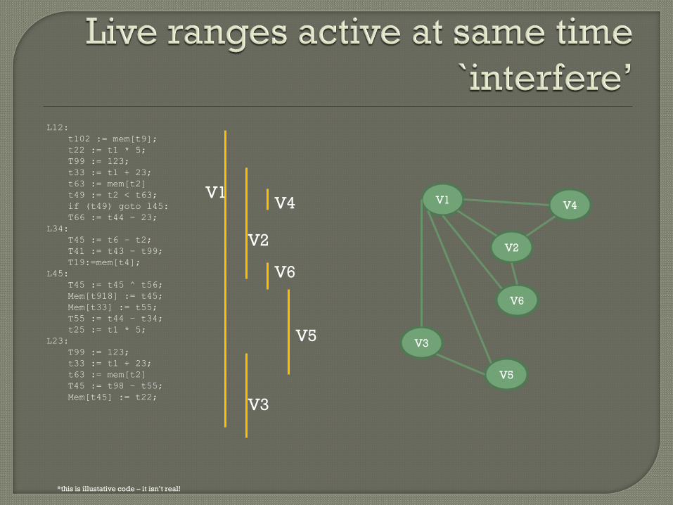
But graph colouring is an NP-complete

problem? How can compilers run in

reasonable time?

Compilers are optimistic – they use an

algorithm which assumes everything

goes to plan. • If this works – great!

• If their optimism was misplaced and they fail,

make the problem easier by reducing live

ranges...

L12:

t102 := mem[t9];

t22 := t1 * 5;

T99 := 123;

t33 := t1 + 23;

t63 := mem[t2]

t49 := t2 < t63;

if (t49) goto l45:

T66 := t44 – 23;

L34:

T45 := t6 – t2;

T41 := t43 – t99;

T19:=mem[t4];

L45:

T45 := t45 ^ t56;

Mem[t918] := t45;

Mem[t33] := t55;

T55 := t44 – t34;

t25 := t1 * 5;

L23:

T99 := 123;

t33 := t1 + 23;

t63 := mem[t2]

T45 := t98 – t55;

Mem[t45] := t22;


V1

L12:

t102 := mem[t9];

t22 := t1 * 5;

mem[fp+4] := t22;

T99 := 123;

t33 := t1 + 23;

t63 := mem[t2]

t49 := t2 < t63;

if (t49) goto l45:

T66 := t44 – 23;

L34:

T45 := t6 – t2;

T41 := t43 – t99;

T19:=mem[t4];

L45:

T45 := t45 ^ t56;

Mem[t918] := t45;

Mem[t33] := t55;

T55 := t44 – t34;

t25 := t1 * 5;

L23:

T99 := 123;

t33 := t1 + 23;

t63 := mem[t2]

T45 := t98 – t55;

t22 := mem[fp+4];

Mem[t45] := t22;

V7

V8

Smaller live ranges means less

interference

Less interference means more chance of

register allocation working.

A few iterations of allocation and spilling

will generally result in a valid register

allocation.

Large data set operations will perform the same operation on multiple elements of data.

Vectorisation allows those operations to be

parallelised, but how ?

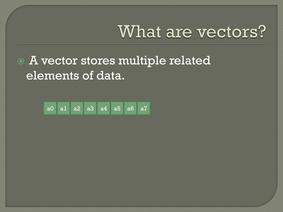
A vector stores multiple related

elements of data.

a0 a1 a2 a3 a4 a5 a6 a7

Combine with another vector in a single

instruction to produce a third vector.

a0 a1 a2 a3 a4 a5 a6 a7

b0 b1 b2 b3 b4 b5 b6 b7

c0 c1 c2 c3 c4 c5 c6 c7

ADD

=

c0 = a0 + b0, c1 = a1 + b1, ...

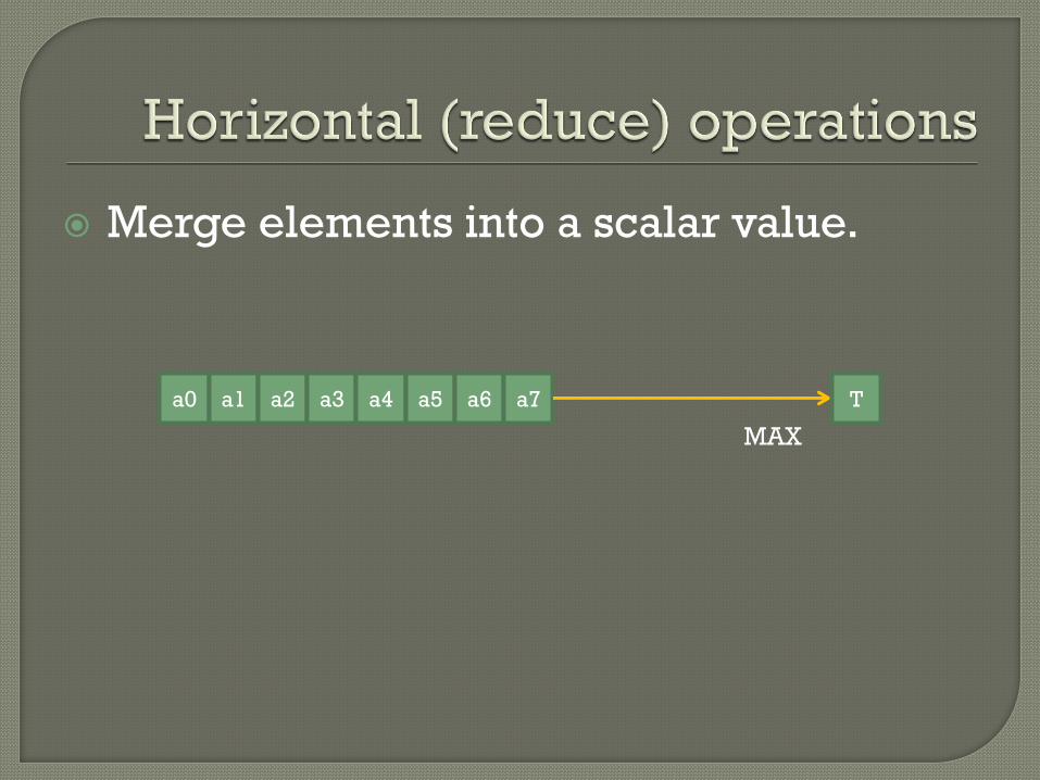
Merge elements into a scalar value.

a0 a1 a2 a3 a4 a5 a6 a7

MAX

T

Vectorisation is important for many types of large data set processing operations.

Vector units (SIMD) are everywhere: • Intel MMX, SSE[1,2,3,4] • PowerPC (Xbox 360) • GPU engines

• ARM 7s (iPhone 5, Galaxy S3)

Automatically generating code to exploit these is therefore very important.

Vector algorithms are important elsewhere, not just compilers – e.g., Map/reduce

Consider a simple loop to find the largest value:

int m = 0;

for (size_t i=0; i!=916; ++i)

m = std::max (m, a[i]);

Try to vectorise this to take advantage of

a vmax instruction, which compares 8 elements at once.

916 (114 * 8 + 4) elements, but vmax works on 8 elements at a time. Split the loop:

int m = 0;

for (size_t i=0; i!=912; ++i)


for (size_t i=912; i!=916; ++i)


Nest another loop inside the first which

operates on 8-elements at a time:

for (size_t i=0; i!=912; i+=8)

for (size_t j=0; j!=8; ++j)

m = std::max (m, a[i + j]);

Introduce more instruction-like operations:

for (size_t i=0; i!=912; i+=8)

{

int* tbase = &a[i];


{

int temp = tbase[j];

m = std::max (m, temp);

}

}

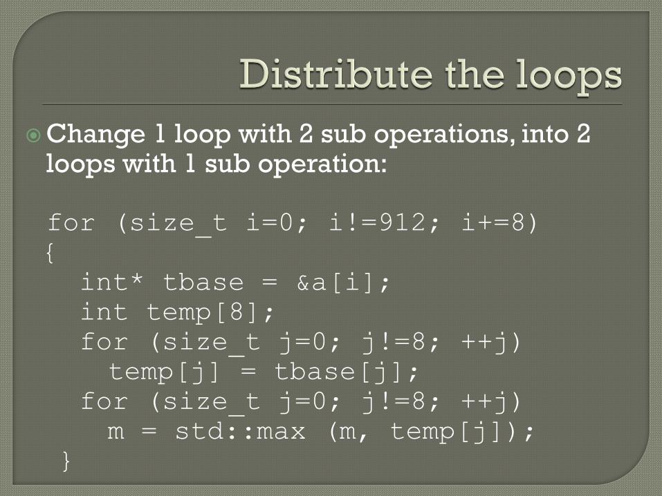
Change 1 loop with 2 sub operations, into 2 loops with 1 sub operation:

for (size_t i=0; i!=912; i+=8)

{

int* tbase = &a[i];

int temp[8];


temp[j] = tbase[j];


m = std::max (m, temp[j]);

}

Replace the sub-loops with their vector

equivalents:

for (size_t i=0; i!=912; i+=8)

{

int* tbase = &a[i];

int temp[8] = vecLoad (tbase);

int localm = vecMax (temp);

m = std::max (m, localm);

}

The loop could then be optimised

further: • Strength reduction/induction

• Loop unrolling

• And so on...

Many loops contain variables whose values are related. By understanding these relationships, and substituting

equivalencies, the loops can run faster.

SOURCE INTERMEDIATE

int32_t *a;

for(size_t i=0; i!=N; ++i)

a[i] = i * 5;

copy 0, i

start:

cmp i, n

beq end

mul i, 5, t0

mul i, 4, t1

add t1, a, t2

store t0, t2

incr i

bra start

end:

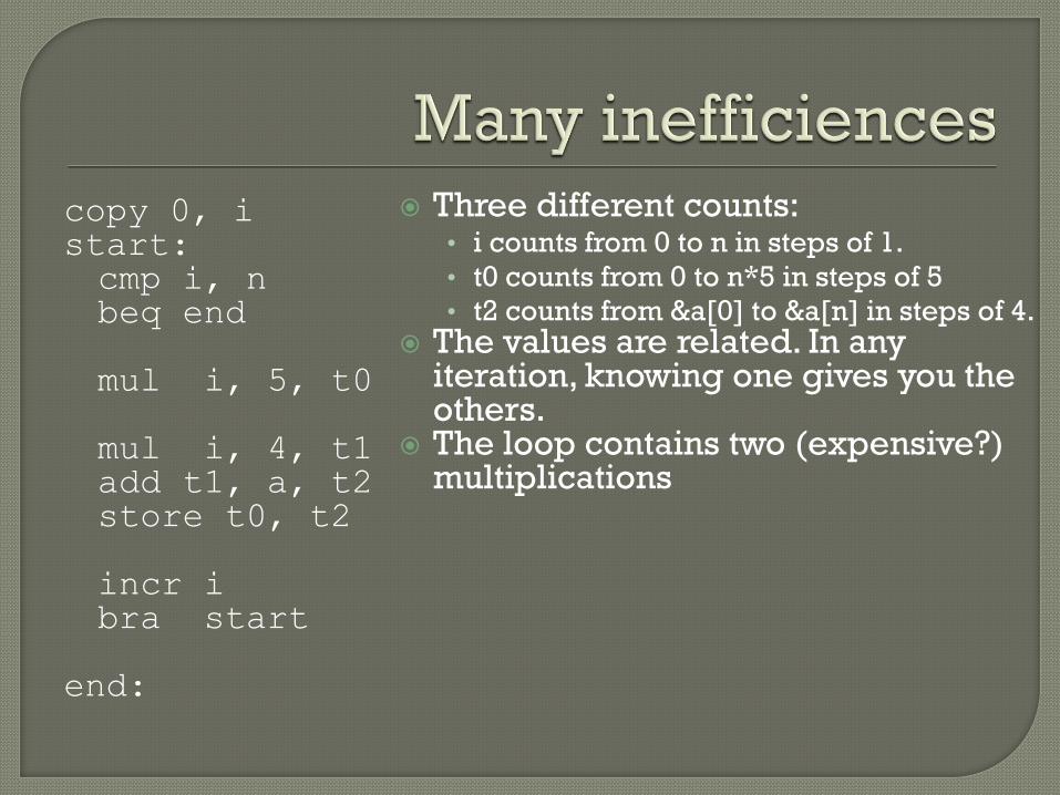
copy 0, i start: cmp i, n beq end mul i, 5, t0 mul i, 4, t1 add t1, a, t2 store t0, t2 incr i bra start end:

Three different counts: • i counts from 0 to n in steps of 1.

• t0 counts from 0 to n*5 in steps of 5

• t2 counts from &a[0] to &a[n] in steps of 4. The values are related. In any

iteration, knowing one gives you the others.

The loop contains two (expensive?) multiplications

copy 0, i copy 0, t0 copy &a, t2 start: cmp i, n beq end add t0, 5, t0 add t2, 4, t2 incr i bra start end:

The values written to a[i] are:

i * 5

Since i is incrementing by one

each iteration, the values

assigned are:

0, 5, 10, 15, ...

So the multiplication can be

replaced by an initialisation, and

an addition in each iteration. As

can the other multiplication.

Also improves ILP.


There are three additions in

the loop now:

• i incremented by 1

• t0 by 5

• t2 by 4

i is used only for controlling

the loop [0..n)

We could equally well use:

• t0 in range [0...n*5)

• t2 in range [&a, &a + 4 * n).


copy 0, t0 copy &a, t2 mul n, 5, t9 start: cmp t0, t9 beq end add t0, 5, t0 add t2, 4, t2 bra start end:

Fewer overall instructions, fewer loop

instructions and also fewer registers.

copy 0, t0

copy &a, t2

mul n, 5, t9

start:

cmp t0, t9

beq end

add t0, 5, t0

add t2, 4, t2

bra start

end:

copy 0, t0

copy &a, t2

mul n, 5, t9

start:

cmp t0, t9

beq end

add t0, 5, t0

add t2, 4, t2

bra start

end:

Too many branches. Branches are expensive:

• Long latency

• Bubbles in the pipeline

• Cause scheduling problems.

You will always need a comparison, so can that close the loop?

A loop with a comparison at the end is a do..while. In source language terms: do {

a[i] = i * 5;

} while (i != n);

But we need to look out for zero iterations too:

if (n > 0)

do {

a[i] = i * 5;

} while (i != n);

}

(Note that the compiler implements this in

intermediate code)

copy 0, t0

copy &a, t2

mul n, 5, t9

start:

cmp t0, t9

beq end

add t0, 5, t0

add t2, 4, t2

bra start

end:

cmp 0, n

beq end

copy 0, t0

copy &a, t2

mul n, 5, t9

start:

add t0, 5, t0

add t2, 4, t2

cmp t0, t9

beq start

end:

Fewer branches. Fewer loop instructions.

fn: .LFB0: testl %edi, %edi jle .L4 leal (%rdi,%rdi,4), %ecx movl $array, %edx xorl %eax, %eax .L3: movl %eax, (%rdx) addl $5, %eax addq $4, %rdx cmpl %ecx, %eax jne .L3 .L4:

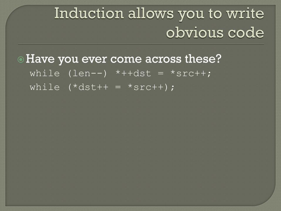
Have you ever come across these? while (len--) *++dst = *src++;

while (*dst++ = *src++);

Have you ever come across these? while (len--) *++dst = *src++;

while (*dst++ = *src++);

They still comes up as recommended. for (i=0; i!=len; ++i)

dst[i] = src[i];

This is more readable, more obvious, and

thanks to induction, strength reduction

and loop inversion, it’s just as fast.

As the compiler gets more clever with

its optimisations, how does the

debugger make sense of it all?

“Debugging is twice as hard as writing the code in the first place. Therefore, if you

write the code as cleverly as possible, you are, by definition, not smart enough to

debug it.” – Brian W. Kernighan

The compiler tells the debugger what it

has generated using DWARF.

DWARF is Debug With Arbitrary Record

Format.

Often stored in an ELF file.

Can be extended to allow for special

features of a compiler or platform.

DWARF is non-intrusive (i.e., the

compiled code doesn’t change)

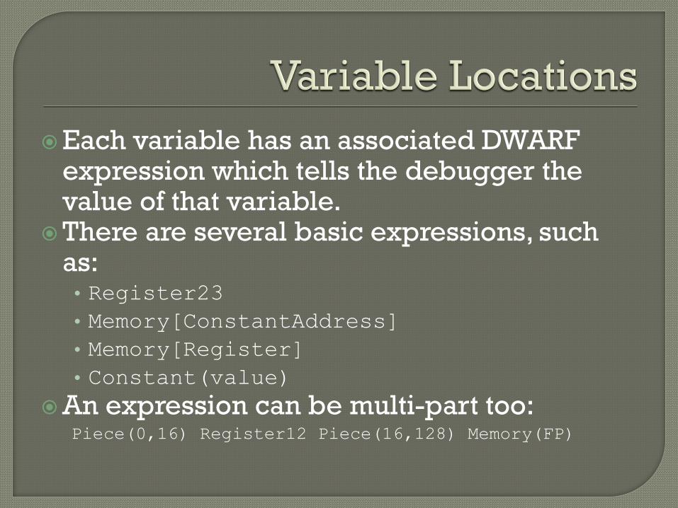
Each variable has an associated DWARF expression which tells the debugger the value of that variable.

There are several basic expressions, such as: • Register23

• Memory[ConstantAddress]

• Memory[Register]

• Constant(value)

An expression can be multi-part too: Piece(0,16) Register12 Piece(16,128) Memory(FP)

The debugger contains a virtual machine,

based upon a stack-engine.

The variable expression elements are

instructions for that virtual machine.

For example, read the contents of a

function argument passed on the stack: RegSP, Constant(12),

Add, Deref







Add, Deref

12356







Add, Deref

12

12356







Add, Deref

12368







Add, Deref

The variable’s value is left.

42

Consider our previous induction-

optimised loop.

The variable i was optimised out of

existence.

However, the debugger can still generate a value for i by running a program: RegT0, Constant(5), Div

Or: RegT2, Constant(&a), Sub, Constant(2), Shr

The virtual machine implementation can do: • Arithmetic (add, sub, etc) • Memory operations (load) • Register operations

• Branching (if/then/else) • More exotic debugger-specific instructions (e.g., Piece).

This allows the compiler to generate programs which reverse the effects of optimisations, to allow sane debug output to be generated.

Special data-types (e.g., built-in linked lists) can be supported by the compiler generating appropriate programs, rather than debuggers having to be extended with extra support.

Hopefully I’ve revealed a little more of

what goes on in a compiler.

The sophisticated algorithms used allow

the programmer to concentrate on

writing clean, understandable, testable,

maintainable code.

Questions?

What is the fastest way to move/copy a

block of memory?

What is the fastest way to move a region of memory? memmove (dest, src, length);

If length is known, and is small, the compiler is allowed to generate direct code to deal with it.

If the compiler can’t deal with it, it will hand off to the run-time library.

The run-time library will often look at the length, the alignment, and choose the best strategy to do the copy (e.g., is a vector engine available). It may even hand off to the OS...

...which is likely to know about the processor type, cache organisation, line sizes, DMA, page mappings, and all sorts of tricks to do this the fastest possible way.

the inner secrets of compilers

Technology

memt2 t45

t55 t55

t45 memt33

t22 t99

t2 t63

t98 t55 t22

memt2 t49

t49 goto l45