Icarus 226 (2013) 999–1019

Contents lists available at ScienceDirect

Icarus

journal homepage: www.elsevier .com/locate / icarus

The inner small satellites of Saturn: A variety of worlds

0019-1035/$ - see front matter � 2013 Elsevier Inc. All rights reserved.http://dx.doi.org/10.1016/j.icarus.2013.07.022

⇑ Corresponding author.E-mail address: pct2@cornell.edu (P.C. Thomas).

P.C. Thomas a,⇑, J.A. Burns a, M. Hedman a, P. Helfenstein a, S. Morrison b, M.S. Tiscareno a, J. Veverka a

a Center for Radiophysics and Space Research, Cornell University, Ithaca, NY 14853, USAb Department of Planetary Sciences, University of Arizona, Tucson, AZ 85721, USA

a r t i c l e i n f o

Article history:Received 22 March 2013Revised 10 July 2013Accepted 13 July 2013Available online 22 July 2013

Keywords:Saturn, SatellitesGeological processesGeophysicsPhotometry

a b s t r a c t

More than a dozen small (<150 km mean radius) satellites occupy distinct dynamical positions extendingfrom within Saturn’s classical rings to the orbit of Dione. The Cassini mission has gradually accumulatedimage and spectral coverage of these objects to the point where some generalizations on surface mor-phology may be made. Objects in different dynamical niches have different surface morphologies. Satel-lites within the main rings display equatorial ridges. The F-ring shepherding satellites show structuralforms and heavily cratered surfaces. The co-orbitals Janus and Epimetheus are the most lunar-like ofthe small satellites. Satellites occupying libration zones (Trojan satellites) have deep covering of debrissubject to downslope transport. Small satellites embedded in ring arcs are distinctively smooth ellipsoidsthat are unique among small, well-observed Solar System bodies and are probably relaxed, effectivelyfluid equilibrium shapes indicative of mean densities of about 300 kg m�3.

� 2013 Elsevier Inc. All rights reserved.

1. Introduction

The smaller (<150 km mean radius) satellites of Saturn occupyseveral dynamical niches: associated with rings (Pan, Daphnis, At-las, Prometheus, Pandora), co-orbiting between the F ring and thelarger satellites (Janus and Epimetheus), orbiting in faint rings or inring arcs (Aegaeon, Methone, Anthe, Pallene), and orbiting librationpoints of larger moons (Telesto, Calypso, Polydeuces, and Helene).Hyperion, the largest irregularly-shaped satellite of Saturn, orbitsbetween Titan and Iapetus, and Phoebe, the next largest, is in a ret-rograde orbit well outside the orbits of the large satellites. Manysmaller objects orbit farther from Saturn (Gladman et al., 2001;Denk et al., 2011); they are not resolved in Cassini images andare not considered in this work.

The small satellites do not experience the internally driven pro-cesses that larger objects do, but the imaging survey by Cassini hasshown distinct differences in morphology among the small objectsthat vary with their orbital and dynamical groupings. This correla-tion suggests that their morphologies, shaped by external ratherthan internal processes, may reveal aspects of the dynamics ofmaterials orbiting close to Saturn. This work examines the mor-phological characteristics of these satellites and outlines some ofthe possible mechanisms that may explain the variations amongobjects that do not suffer effects of internal activity.

The small satellites generally are expected to be fragments orrubble-like assemblages. The higher-density example of Phoebemay be an exception (Johnson et al., 2009; Castillo-Rogez et al.,

2012) as its shape suggests an early relaxation to a nearly sphericalobject, possibly the result of internal heating. Nearly all of theseobjects have been imaged by Cassini at pixel scales of <300 m(Table S1), although not over their entire surfaces. These resolu-tions allow comparison of shapes, surface features, photometry,and colors. The basic shapes, densities, and some surface featuresof the small saturnian satellites have been discussed in Porcoet al. (2005) (Phoebe), Porco et al. (2007) (ring satellites), and Tho-mas (2010). With the exception of Phoebe, all of these objects thathave measured masses appear to have mean densities consistentwith highly porous water ice. Other components are almost cer-tainly present, but likely constitute onlysmall amounts (Filacchioneet al., 2010; Buratti et al., 2010). Model porosities assuming a soliddensity of 930 kg m�3 (appropriate for water ice) are �30–60%.Addition of a denser component would increase these modelporosities.

This paper uses Cassini Imaging Science Subsystem (ISS; Porcoet al., 2004) data obtained through mid-2012 to update the shapesand characteristics of these small satellites. Notably better datawill not be obtained until 2015. We deal with all the inner group-ings of the small saturnian satellites, but concentrate on the ring-arc embedded satellites and on the Trojan satellites co-orbitingwith Tethys and Dione.

2. Data and methods

All images used are from the Cassini Imaging Science Subsystem(Owen, 2003; Porco et al., 2004); most are from the Narrow AngleCamera (NAC) which has a pixel scale of 6 km at a million kmrange. Shape models of the satellites have been gradually improved

1000 P.C. Thomas et al. / Icarus 226 (2013) 999–1019

with data from multiple flybys at a variety of resolutions, viewingangles, and phase angles. The orbit of the Cassini spacecraft haschanged during the mission to support different goals, some ofwhich require high inclinations that lead to periods of months oryears between close imaging of small satellites.

Stereo control point solutions are the basis of the shape modelsand libration studies. Control points are marked manually onimages covering as wide a range of observer geometries as possiblewith the POINTS program (J. Joseph; in Thomas et al. (2002)Tho-mas et al. (2002)). Some additional control points have been addedthrough automated image matching, but these are a small minorityof the points that are used. Resolutions of the images used varygreatly due to the nature of the different flyby trajectories. Resid-uals of the control point solutions (predicted vs. observed imagelocations) are typically 0.3–0.4 pixels. Shape models are fit to thestereo points, and modified based on limb profiles. The shape mod-els are derived in the form of latitude, longitude, radius at 2� inter-vals in latitude and longitude (Simonelli et al., 1993) but for somepurposes can be converted to more evenly spaced x, y, z triangularplate models. In some cases Saturn-shine or silhouettes of the sat-ellites in front of Saturn provide crucial coverage of limbs or of con-trol points. Description of the techniques are in Simonelli et al.(1993) and Thomas et al. (2007a).

Solving for the control points requires knowledge of the instan-taneous orientation of the object. Correctly predicting the satel-lites’ orientations requires accurate orbital and rotational data,including information on any forced libration (Tiscareno et al.,2009). Our model for Helene’s orientation is of the same form asthat described by Tiscareno et al., based on the moon maintainingsynchronous rotation (even as the orbit frequency changes due tothe co-orbital resonance) with additional librations of variableamplitude that track the instantaneous orbit frequency. More de-tailed dynamical analysis (Noyelles, 2010; Robutel et al., 2011a)confirmed in the case of Janus and Epimetheus that there are noobservable deviations from the Tiscareno et al. model, as expectedfor a moon whose rotational dynamics are dominated by in-planeforced librations due to its non-spherical shape. Although Robutelet al. (2011b) recently presented a detailed dynamical analysis ofthe orientation of Helene, we choose for this work to continueusing the Tiscareno et al. model, which gives sufficient precision,is easy to implement, and is physically intuitive. The control-pointsolutions for Helene suggest any forced libration is <1� (Fig. S3).Predictions on possible forced librations based on the shape modelalone are limited both by necessary assumptions of a homoge-neous interior as well as low-resolution views of some longitudes,and the presence of an as-yet unimaged region including the northpole. The model moment ratio from the current shape model for(B � A)/C is 0.014, which would predict physical librations of<0.1�, a value we are far from being able to detect.

For Calypso and Telesto, we obtained sufficiently precise controlpoint results from a model assuming a constant rotation rate, asany librations were undetectable probably due to their smalleramplitudes of libration in the co-orbital resonance (Oberti and Vi-enne, 2003; Murray et al., 2005).

For the more ellipsoidal objects, shapes are determined by mea-surement of limb coordinates for an analytical ellipsoidal fit. Scansare taken in images along line or sample directions and the posi-tion of a sharp bright edge is modeled in steps of 0.05 pixels; thelimb coordinate is selected as the best match of predicted and ob-served brightness. The line and sample coordinates so obtained arecorrected for spacecraft range and optical distortion to relativepositions in km in the viewing plane. An ellipsoid is then fit toviews from different directions, allowing the three ellipsoidal axesand the coordinate center to vary. The uncertainties in range andorientation of the image are assumed to induce errors in the shapethat are small compared to other sources of error; see Dermott and

Thomas (1988) for a discussion of the effects of such errors on thesolutions. Precision of the limb measurement is commonly betterthan 0.1 pixel. The uncertainty in ellipsoidal solutions dependson the limb topography (roughness, or how close to an ellipsoidit is), resolution, and the spread of viewpoints that constrain thesolution.

Crater counting and feature mapping are done interactivelywith the POINTS program. Features are mapped using manuallystretched images. Locations of mapped points are the projectionof single points, or centers of ellipses (such as crater rims) on theshape model in particular images. Data are stored in text files thatinclude body-centered and image locations, and image and lightinginformation. Past experience in mapping irregular objects showsthat crater counts are reliable down to diameters of 5–7 pixelsand in images above 45� phase. Mapping coordinates use West lon-gitudes, per the IAU rules for satellites (Archinal et al., 2011), and0�W is on the (on average) sub-Saturn point. Topography is de-scribed by dynamic heights (Hd; Vanicek and Krakiwsky, 1986;Thomas, 1993) which are similar to, but not identical with, heightsabove an equipotential. Hd is the potential energy at a point on thesurface divided by an average surface acceleration. The potentialenergy calculation accounts for the irregular shape of the body’smass assuming uniform density, and rotational and tidalaccelerations.

For our photometric work we first radiometrically calibratedthe ISS images with the CISSCAL computer program, which is avail-able through the Planetary Data System (PDS). Details of the ISSCamera calibration are given in West et al. (2010), Porco et al.(2004), and the CISSCAL User’s Manual (http://pds-rings.seti.org/cassini/iss/software.html). In the calibrated images, pixel DN val-ues are scaled to radiance factors, I=f , where I is the specific scat-tered intensity of light and pf is the specific plane-parallel solarflux over the wavelength range of the filter bandpass. We rely onthe four ISS NAC multispectral filters that were most frequentlyused during close-flybys as well as distant imaging of the satellites;CL1–CL2 (611 nm), CL1–UV3 (338 nm), CL1–GRN (568 nm), andCL1–IR3 (930 nm). Sampling of whole-disk and disk-resolved pho-tometric measurements follows the approach of Helfenstein et al.(1994). In general, disk-resolved measurements were obtainedonly from images for which the diameter of the object in pixelswas larger than 100 pixels. Local angles of incidence (i), emission(e), and phase angle (a) on the surfaces of the satellites were ob-tained using the appropriate satellite shape model and correctedcamera pointing geometry via the POINTS program, cited earlier.From each image, the pixel-by-pixel disk-resolved radiance factorswere measured and binned into 10� increments of photometric lat-itude and longitude.

3. Ring satellites

3.1. Pan, Atlas, Daphnis

These objects have been studied previously by Porco et al.(2007) and Charnoz et al. (2007). Pan (mean radius Rm, of 14 km)within the Encke gap of Saturn’s A ring, and Atlas (Rm = 15 km), justoutside the A ring, have been imaged at sufficient resolution toshow distinct equatorial ridges giving these somewhat elongatedobjects ‘‘flying saucer’’-like shapes. (Fig. 1, Table 1). Daphnis(Rm = 3.8 km) is also elongate and although it is less well-resolvedthan Pan and Atlas in terms of pixels/radius, it does have low-lat-itude ridge and is also somewhat saucer-shaped in that the a and baxes are both fractionally much larger than the c axis. These threeobjects rotate at least approximately synchronously with theirorbital periods; synchroneity must be estimated by congruenceof shape models at scattered, low-resolution views. Atlas is within

Fig. 1. Montage of primary study objects. Best images scaled to 250 m/pixel (seeTable 1). Top row: Calypso: N1644754596; Telesto: N1507754947; Helene:N1687119756. Second row: Pallene N146910452; Methone N1716192103. Thirdrow: Janus: N164934235; Epimetheus: N1575363139. Fourth row: Prometheus:N1640497752; Pandora: N1504613650. Bottom row: Atlas N1560303820; DaphnisN1656999330; Pan N1524966847. Note that the Pan image is partly obscured byring material (just above the middle).

P.C. Thomas et al. / Icarus 226 (2013) 999–1019 1001

�15� of synchronous over 4 years; Pan �20� over 4.5 years; Daph-nis �30� over 3.5 years. Geometrically all of these values couldhave multiples of 360� added. The elongate shapes and low meandensities (Table 1) indicate that the surfaces of these three moonshave very low escape velocities, and crudely approximate shapes ofRoche lobes (Porco et al., 2007). Consequently, additional accretedmaterial would be only loosely bound. This property is also foundon Mars’ Phobos (Dobrovolskis and Burns, 1980) and Jupiter’sAmalthea (Burns et al., 2004). Charnoz et al. (2007) note that thelatitudinal extent of the equatorial ridge of Atlas is close to therange of vertical motion of the satellite relative to the ring. Theymodel accretion of the equatorial ridges from ring particles. Theconsiderable range of dynamic heights (Hd) on the surfaces ofring-related satellites is not reduced by modeling the presence of

Table 1Properties of irregularly-shaped saturnian satellites.

Satellite A (km) B (km) C (km) Rm (km) M

Pan 17.2 ± 1.7 15.4 ± 1.2 10.4 ± 0.9 14.0 ± 1.2 0Daphnis 4.6 ± 0.7 4.5 ± 0.9 2.8 ± 0.8 3.8 ± 0.8 .Atlas 20.5 ± 0.9 17.8 ± 0.7 9.4 ± 0.8 15.1 ± 0.8Prometheus 68.2 ± 0.8 41.6 ± 1.8 28.2 ± 0.8 43.1 ± 1.2 1Pandora 52.2 ± 1.8 40.8 ± 2.0 31.5 ± 0.9 40.6 ± 1.5 1Epimetheus 64.9 ± 1.3 57.3 ± 2.5 53.0 ± 0.5 58.2 ± 1.2 5Janus 101.7 ± 1.6 93.0 ± 0.7 76.3 ± 0.4 89.2 ± 0.8 18Aegaeon 0.7 ± 0.05 0.25 ± 0.06 0.2 ± 0.08 0.33 ± 0.06Methone 1.94 ± 0.02 1.29 ± 0.04 1.21 ± 0.02 1.45 ± 0.03Anthe 0.5Pallene 2.88 ± 0.07 2.08 ± 0.07 1.8 ± 0.07 2.23 ± 0.07Telesto 16.3 ± 0.5 11.8 ± 0.3 9.8 ± 0.3 12.4 ± 0.4Calypso 15.3 ± 0.3 9.3 ± 2.2 6.3 ± 0.6 9.6 ± 0.6Polydeuces 1.5 ± 0.6 1.2 ± 0.4 1.0 ± 0.2 1.3 ± 0.4Helene 22.5 ± 0.5 19.6 ± 0.3 13.3 ± 0.2 18.0 ± 0.4Hyperion 180.1 ± 2.0 133.0 ± 4.5 102.7 ± 4.5 135 ± 4 56Phoebe 109.4 ± 1.4 108.5 ± 0.6 101.8 ± 0.3 106.5 ± 0.7 8

Masses for Janus, Epimetheus, Atlas, Prometheus, and Pandora are from Jacobson et al. (20Thomas et al., 2007b. Mass of Phoebe is from Jacobson et al. (2006). Masses are in units

cores. Models of these objects with dense (900 kg m�3) cores andvery porous (150 kg m�3) mantles cannot be discriminated fromhomogeneous interior models (Porco et al., 2007). (Here we use‘‘core’’ to denote a denser central region, not implying any thermaldifferentiation process.) The models do show a large range of sur-face gravity (for homogeneous models; Table 1) that is typical ofelongate, low-density, rapidly rotating objects. For these objects,all surface accelerations are still inward; that is, material is boundgravitationally to their surfaces.

Of these three objects, only Atlas has image coverage of suffi-cient resolution (250 m/pixel) to allow some discussion of surfacemorphology. The equatorial ridge is smoother than terrain at high-er latitudes, but is not gravitationally flat: it has substantial slopes.For a homogeneous interior, relative dynamic heights along theequator vary by several km; the local acceleration and escapespeeds (Fig. 2) also vary substantially around the equator. Both At-las and Pan have relative gravitational topography that is largecompared to their radii. The equatorial ridge on Atlas is gravita-tionally several km higher than the surface at mid-latitude regions,and is flanked by slopes relative to gravity of �20�. This greater rel-ative height of the equatorial region is different from that of someasteroids (Ostro et al., 2006; Harris et al., 2009) where equatorialridges formed on rapidly spinning objects are gravitationally lowand accumulate materials moving from gravitationally higherareas at greater latitudes. The large range of Hd on Atlas and Pansuggests that their shapes are not close to gravitational equilib-rium conditions, no matter what the shaping mechanism, be it sur-face flow or accretion from outside. Extra accretion from ring-planematerial may explain the ridges (Charnoz et al., 2007). If the ridgesare composed of material less dense than a core, the relative grav-itational height of the ridge crest would be greater than for thehomogeneous model.

Topography on Atlas south of �30� has a lumpy appearancewith some subtle, crudely east–west ridges �2 km wide (N–S)and 3–5 km long (Fig. 2). It may have as many as five impact cra-ters over 1 km in diameter in this area; these require viewing mul-tiple stretches of the images and blinking images to see roundforms that reproduce image-to-image (Fig. S1). Hirata and Miyam-oto (2012) identified only one possible crater on Atlas, differentfrom those mapped here. If these are indeed impact craters theirmuted topography suggests surface processes that erode and redis-tribute materials are nearly rapid enough to match crater forma-tion rates. If they are not craters the conclusion is simply thatrecent rates of surface processes completely erase craters.

ass q (kg m�3) g (cms�2) best (km/pixel) Pixels/radius

.495±.075 430 ± 150 0.01–0.18 1.2 120077±.0015 340 ± 260 0.01–0.04 0.45 80.66 ± 0.045 460 ± 77 0.02–0.19 0.25 605.95 ± 0.15 470 ± 44 0.13–0.58 0.20 2173.71 ± 0.19 490 ± 60 0.26–0.60 0.31 1312.66 ± 0.06 640 ± 62 0.64–1.1 0.22 3239.75±.0006 630 ± 30 1.1–1.7 0.18 496

0.10 30.03 545.3 <10.16 14

– 0.059 210– 0.13 74

0.41 70.042 424

1.99 ± 5 544 ± 50 1.7–2.1 0.014 964029.2 ± 1 1638 ± 33 3.8–5.0 0.013 8190

08). Masses for Pan and Daphnis are from Porco et al. (2007). Mass of Hyperion fromof 1019 g.

Fig. 2. Cross sections and gravitational topography (dynamic heights, Hd) of Atlas and Pan. Top: images from Fig. 1 of Atlas and Pan. Second row: cross sections, viewingequator profile (largest), and 90–270�W longitude profiles (smaller of inner sections), and 0–180�W longitude profiles (more elongate of inner profiles). Third row: Hd along90–270�W longitude lines. Bottom row: profiles along equators. Note that vertical exaggerations vary in Hd plots.

1002 P.C. Thomas et al. / Icarus 226 (2013) 999–1019

Pan’s equatorial ridge is relatively smaller than is Atlas’ (Fig. 2).Image resolution of Pan is not sufficient to detect any textural con-trasts between the equatorial region and higher latitudes. Daphnisis only a few pixels across in the image data, it is elongated, but nosurface features can be resolved.

3.2. Prometheus and Pandora

Prometheus and Pandora shepherd the F ring, and having meanradii of 43 and 41 km, respectively, are far larger than Atlas andPan. The mean densities of the F-ring shepherds are constrainedto be slightly below 500 kg m�3 for both objects (Table 1). Theseelongate objects have substantial crater densities (see Section 6.5)and are more irregular and varied in form than are Pan and Atlas(Figs. 1 and 3). Pandora is a typical cratered, elongate, small object

with some morphologic distinctions. First, it has grooves up to�30 km in length in the trailing part of the northern hemisphere,most in a pattern of roughly parallel members oriented �30� tothe intermediate axis (Morrison et al., 2009). Second, it has severalvery shallow craters, some probably partly filled by ejecta. Othercraters are shallow, elongate, and relatively young, similar inappearance to those common on Hyperion (Thomas et al.,2007a,b; Howard et al., 2012) (Fig. 1).

Prometheus is a heavily cratered object; much of its surface ap-pears similar to those of Janus and Epimetheus. However, it is dis-tinguished by global topography that suggests division into twoterrains, one lower than the other and possibly representing an ex-posed inner core region. These terrains are bounded by long scarps(Fig. 3), features not seen on other small satellites. The only possi-ble analogy on another small satellite might be the boundaries

Fig. 3. Prometheus, showing possible expression of core. (A) Image N1643261394,from 19�N, 238�W, north is approximately up. (B) Image N1640497752 from 1�N,100�W, north is approximately up. Image processing includes some high-passfiltering. (C) Map of exposure of distinct, lower terrain, possibly an exposed innercore or other distinct material. Major craters schematically mapped.

P.C. Thomas et al. / Icarus 226 (2013) 999–1019 1003

between the smooth equatorial regions of Atlas and the rougher,higher latitudes (Section 3.1). The lower terrain on Prometheus isdensely cratered (Fig. 3); thus, if Prometheus is a partially delami-nated object, that event happened at a large cratering age. We haveapproximated the shape of the region that might be an exposedcore by interactively trimming the overall shape model to includesmooth extensions of the lower terrain. The lower surface is ex-posed chiefly between longitudes 20–100�W and 170–260�W(Fig. 3c). The estimated volume of the putative core is2 � 105 km3, about 2/3 the whole object’s volume of3.4 � 105 km3. The putative core is roughly an ellipsoid of semi-axes 60.5, 34.7, and 25.5 km.

4. Co-Orbitals Janus and Epimetheus

Janus (Rm = 89 km) and Epimetheus (Rm = 58 km) make upnearly 90% of the mass of the inner small satellites of Saturn (Ta-ble 1). They exchange orbits every 4 years (Dermott and Murray,1981a,b; Yoder et al., 1989) and Epimetheus has been shown tohave a forced libration of �6� (Tiscareno et al., 2009). Early shapemodeling work for Janus had suggested an offset of the minimummoment of inertia from Saturn-facing direction (Tiscareno et al.);however, the updated shape reported here has a moment offsetof less than 1�, indicating there is no need to invoke substantialinternal inhomogeneities. The mean densities of these two satel-lites are indistinguishable (640 ± 60 and 630 ± 30 kg m�3) and arehigher than those of the smaller satellites for which density data

have been obtained (possible exception in upper limits of Aegaeon;see Section 5). These two moons are marginally more dense thanHyperion (544 ± 50 kg m�3). The surfaces are heavily cratered (Sec-tion 7); both objects show a variety of crater degradation states aswell as some ponding of materials in crater floors (Morrison et al.,2009; see especially Epimetheus in Fig. 1).

Epimetheus has grooves 5–20 km in length averaging �1 km inwidth that are visible in the highest resolution images of the southpolar region (Morrison et al., 2009). Some of these grooves displaystraight-walled morphology suggestive of graben, and thus indi-cate near-surface faulting. Most of these grooves trend parallel tothe intermediate axis of Epimetheus, similar to some of the prom-inent grooves on Phobos’ northern hemisphere and are distinctlydifferent from the scattered patterns of grooves on asteroids Erosand Gaspra. At least one of the graben-like grooves cuts the rimof a 5-km crater.

5. Embedded satellites: Aegaeon, Pallene, Methone

Four small satellites lie beyond the orbits of Janus and Epime-theus: Aegaeon interior to Mimas and within the G ring; and Meth-one, Anthe, and Pallene orbiting between Mimas and Enceladus.These latter three satellites all have associated rings or ring arcs(Hedman et al., 2009). Anthe is only �0.5 km in radius, and isnot spatially resolved. Aegaeon (Rm = 0.3 km) is resolved a few pix-els in width. Pallene (Rm = 2.2 km) and Methone (Rm = 1.5 km) havesufficiently good imaging data (Fig. 4) for accurate size measure-ments and that show them to be morphologically distinct fromother small saturnian moons, and from any previously imagedsmall satellite, small asteroid, or comet nucleus.

5.1. Shapes

Results of shape fitting are given in Table 2. Aegaeon was seenin only one flyby in images of 91–127 m/pixel spanning �22� inviewing angles. The images of Aegaeon (Fig. S2) are too small forour standard limb-finding software (the few pixels on the bodysubstantially change brightness approaching the limb). The shapewas obtained by matching expanded images of four views(Table S1) with ellipsoidal shape models changing in 50-m steps.Additionally, the high latitude of the viewpoints means the c axisis poorly constrained (largely by the terminator). We estimatethe uncertainty in the fit axes at 0.08, 0.09, and 0.1 km for the a,b, and c axes, respectively. These uncertainties are large fractionsof one pixel.

The disks of Pallene and Methone are large enough (Fig. 4) thatthe standard limb-fitting and error estimation are feasible. Theallowable range of fit ellipsoidal axes is obtained by allowing theresiduals (rms) to increase by 0.12 pixels (accuracy of this softwaredetermined from measurements of objects with independent,high-resolution shapes) above the minimum value. This evaluationgives uncertainties of 0.07 km for all Pallene axes. Methone’s shapehas calculated uncertainties (considered one sigma) of 0.02, 0.04,and 0.02 km for the a, b, and c axes, respectively. Note thatalthough the views of Methone (Table 1) are only slightly betterof the a axis (best view would be 90� from an axis) than of the baxis, the shorter b axis means that it affects projected ellipses lessthan does the a axis, hence the much greater calculated uncer-tainty in the b axis of Methone.

5.2. Inferred mean densities

We test whether the ellipsoidal shapes of these objects are con-sistent with effectively fluid, equilibrium shapes. Below in Sec-tion 5.5 we examine the more general problem of interpreting

Fig. 4. Views of Pallene and Methone. Pallene shown in left set of five panels; km scales vary. Upper left image includes Saturn shine. Images with bright background aretransit views. Right side, Methone image N1716192103, phase angle 63�. Spots are not reproduced image to image.

Table 2Characteristics of embedded moons Aegaeon, Methone, and Pallene.

Dimensions (km)

a b c Rm ± F

Ellipsoidal fits of shapes of embedded moonsAegaeon 0.70 0.25 0.20 0.33 0.05 0.06 0.08 0.10Methone 1.94 1.29 1.21 1.45 0.02 0.04 0.02 0.11Pallene 2.88 2.08 1.84 2.23 0.07 0.07 0.07 0.23

Density (kg m�3) minDHd (km) limitDHd (km) qmin (kg m�3) qmax (kg m�3)

Inferred mean densities of embedded moonsAegaeon 540 0.035 0.070 410 (418) 700 (695)Methone 310 0.008 0.020 280 (288) 330 (324)Pallene 250 0.071 0.142 190 (194) 340 (338)

Density (kg m�3) g (cm s�2) Escape (cm s�2)

Gravity of embedded moonsAegeon 540 0.0093–0.0127 2–17Methone 310 0.0081–0.0130 19–87Pallene 250 0.0106–0.0162 27–107

1004 P.C. Thomas et al. / Icarus 226 (2013) 999–1019

shapes of small, ellipsoidal satellites and asteroids, and explainwhy fluid-like behavior on geological time scales is an appropriateapproach for these objects. If they have behaved geologically as flu-ids, inferences of mean densities may be made. Fluid-like behavioron geological times for these objects could involve any processesthat disperse or transport material at the surface, and need onlyoperate over depths of major craters on the body.

Fluid equilibrium shapes (unless otherwise stated, ‘‘equilib-rium shape’’ is used as a fluid equilibrium; possible non-fluidequilibrium shapes are discussed in Section 5.5) of rapid rotatorsand low density objects are more prolate than the classicalapproximation with the shape parameter F = (b�c)/(a � c) = 0.25(Chandrasekhar, 1969; Dermott, 1979). Mimas, a slightly fasterrotator than the arc-embedded moons, with a density of1150 kgm�3 has an equilibrium F of 0.21 (Thomas et al.,2007a,b). Because the exact equilibrium shape depends uponthe mean density we test how much the observed shapes devi-ate from an equipotential surface as a function of assumed meandensity. Using ellipsoid models of 3� resolution, we assumehomogeneous interiors of varying density, and calculate the po-tential energy over the surface accounting for the distributedmass, rotation, and tidal effects (Thomas, 1993). If a particularmean density yields a very small range of dynamic heights(DHd), the object may be acting as a relaxed fluid.

Table 2 gives the mean densities inferred from the minimumDHd. Uncertainties in the inferred density may be calculated inmultiple ways. One method is to do the DHd calculation by allowingthe shape models to change within observational errors and findingthe range of densities covered by changing minima in DHd. This ap-proach gives density uncertainties of 50, 20 and 10 kg m�3 for Ae-geon, Pallene, and Methone, respectively. We consider thesevalues too optimistic, as they are substantially smaller than thephysical measurement uncertainty. Our adopted approach usesthe range of uncertainty in DHd values induced by the range of pos-sible shapes, and the consideration that the ideal situation wouldhave a DHd of 0 at the appropriate mean density. Because Methonehas a best fit DHd of only 8 m, for this object we test the range of Hd

induced by the allowable range of the shape. The allowable range ofshape for Methone (Table 2) produces a maximum range of Hd of18 m, which we round up to 20 m DHd as the allowable value forMethone. Mean densities that yield 20 m or less DHd for the nomi-nal shape of Methone are 288–324 kg m�3, which we round to thewider range values of 280–330 kg m�3. Pallene and Aegeon are lesswell measured, and we thus simply allow the range of DHd to dou-ble from its minimum. The resulting inferred mean densities are gi-ven in Table 2, and the plots of Hd as a function of model meandensity are shown in Fig. 5. We consider the Table 2 values to bereasonable estimates of 1-sigma uncertainties in the mean

Fig. 5. Range of calculated dynamic heights for Aegaeon, Methone and Pallene as afunction of mean density. Dots show inferred limits of acceptable solutions (seetext). The somewhat segmented shapes of the curves reflect the changing loci onthe surface of the minimum Hd which affects the incremental change in averagegravity and hence the calculated DHd range.

P.C. Thomas et al. / Icarus 226 (2013) 999–1019 1005

densities if the bodies are homogeneous and if they act as fluidsover geological timescales, and if the shapes were set at the currentorbital distances from Saturn.

We list in Table 2 the gravitational accelerations at the surfaceof the satellites and approximate ranges of escape velocities. Therange of net surface accelerations arises from variations in radiiand in rotational and tidal accelerations across the objects. ‘‘Es-cape’’ velocities have been calculated by tracking test particles(methods given in Thomas (1998)) launched radially from pointsacross the surface, in velocity magnitude increments, and settingescape velocity for a particular site when the particle either staysaloft more than ½ orbital period or reaches 10 mean radii dis-tance. Of course particles barely escaping will reimpact at somepoint, but this is a convenient measure for when materialachieves a different ‘‘sedimentary’’ regime. Velocity vectors withdifferent orientations would expand the range of calculated ‘‘es-cape’’ speeds as well.

Fig. 6. Possible core configurations and properties of Methone with its nominalshape. (a) Minimum range of Hd over the surface as function of spherical core size.(b) Mean density and mantle density needed to produce the minimum DHd for eachcore size model. (C) Core mass fraction for each core size.

5.3. Possible non-homogeneous interiors

Perfectly homogeneous interiors of these small satellites mightbe considered unlikely given some views of small objects, such asAsteroid 25143 Itokawa (Fujiwara et al., 2006), Atlas (Porco et al.,2007; Charnoz et al., 2007), and the expectation of either impactfracturing, or accretion of particles of various sizes and mean den-sity that likely follow from differences in collisional history (Porcoet al., 2007). The possible presence of denser cores that have actedas ‘‘seeds’’ for later accumulation invite tests of what the observedshapes would imply for equilibrium properties. We first note that aparticular ellipsoidal equilibrium form has a lower mean density ifcentrally condensed than if it is homogeneous (Dermott, 1979).Thus, if the interpretation of a relaxed fluid state is correct, Meth-one must have some material of density less than 330 kg m�3 evenif it has relatively denser material at depth. Likewise, Pallene andAegaeon would have material equal to, or less than, their calcu-lated maximum mean densities. Secondly, we note that any denser

interiors are unlikely to be simple shapes, and thirdly, models arenot unique but do show trends and limits.

The shape of Methone is the most accurately known of the arc-embedded objects, and thus we use it as an example of the kinds ofmass distributions possible in these objects if they have densercores. To test how the current shape of Methone may relate to acentrally condensed body, we assume a spherical core of density660 kg m�3: this density is twice the inferred upper homogeneousdensity limit of Methone and is similar to the bulk density of Janusand Epimetheus (Table 1). Computationally, the potential from acentered sphere of a particular size and density equal to(660 � 310) kg m�3 is added to the homogeneous solution andthe same potential energy calculations are made for points onthe surface. We initially use the nominal shape (semi-axes of1.94, 1.29, 1.21 km) varying the core size, and find the mantle den-sity that gives the smallest DHd. These results, and the propertiesof the resulting models, are shown in Fig. 6. Very small cores arenot detectable. Allowable solutions with DHd of 20 m or less applyto core radii of 0.65 km with a core mass fraction of 0.25, and man-tle density of 200 kg m�3. Thus our solution of Methone allows for,and cannot distinguish among, core mass fractions of less than�0.25. Small cores with density of >660 kg m�3, or larger coreswith lower mean densities, allow a range of surface material den-sities of �200–330 kg m�3 for this object. A very large core with

1006 P.C. Thomas et al. / Icarus 226 (2013) 999–1019

only a very thin covering would necessarily have a mean densitylittle different from the homogeneous case even if the thin surfacelayer has properties different from the mean.

Fig. 8. Limb profiles from small objects. Vertical exaggeration = 2. These are radialresiduals of limb profiles fit by ellipses; these are not gravitational topography.Data: Phobos, Viking image 854a62, 24.0 m/pxl, a = 45.2�; Deimos Viking image507a01, 32 m/pxl, a = 32.4�; Wild 2 2079we02, 24.2 m/pxl, a = 72.2�; Tempel 1mv0173728278, 28.5 m/pxl, a = 63.4�; Hartley 2 mv0342149134, 22.0 m/pxl,a = 83.1�; Methone N1716192103, 27 m/pxl; a = 63�.

5.4. The surfaces of Aegaeon, Pallene, and Methone: topography

Is the smooth surface of Methone (and Pallene and Aegaeon)unusual for small bodies? If so, what does that characteristic im-ply? The limb residuals are plotted for Pallene and Methone inFig. 7; comparison plots for other small objects with similar reso-lution data are shown in Fig. 8. Methone clearly occupies a differ-ent roughness regime from the comparison objects. Anothersimple method of comparison is to calculate the supported topog-raphy in terms of qgh (density � gravity � height). We use the max-imum gravity calculated for each body. The density we take is thebody’s mean density, realizing that surficial materials may differ.For the height to consider for objects with known mean densitiesand good shape models, we calculate the range of Hd over areasof radius 0.1Rm. For the small ‘‘egg’’ satellites, we simply use theminimum DHd calculated for the whole object (these are roughlyconsistent with the deviations of limb topography). The tabulationof these admittedly rough measures are in Table 3. The egg satel-lites and comet nuclei have the lowest supported loads; satellitessuch as Atlas and Telesto support �700 times the loads calculatedfor Methone. The loads as a function of object mean radius are plot-ted in Fig. 9. Objects other than Pallene and Methone and the threecomet nuclei give a linear slope of 1.8, close to that expected fromsimply scaling shapes up (slope of 2) as g and h would both scalelinearly with radius. The arc satellites and comets lie below theextrapolation from the other bodies.

Interior pressures on these objects are low; central pressure in ahomogeneous Methone of mean density 310 kg m�3 would be�30 Pa. The �100 fold difference in the product of surface gravityand mean density between Janus and Methone means that pres-sures deep within Methone, a few hundred m, are equivalent tothose at a few m depth on Janus, or a few cm depth on the Earth’sMoon. The ability of these objects to sustain high porosity is notsurprising.

The smoothness of Methone compared to other saturnian ob-jects is shown in Fig. 10. The surfaces are compared at 42 m/pixelas the best pixel scales on any small satellite except Methone(27 m/pixel). In these images, at roughly comparable phase angles,it is clear that Methone is distinct. The other objects, except thesample of Helene, have variations on crater topography, which is

Fig. 7. Limb residuals for Methone (left) and Pallene (right). Note different scales for Met161 m/pixel. Top: Pallene image is 460 m/pixel, bottom is 220 m/pixel.

lacking on Methone. The regions selected for Fig. 10 on the largerobjects were specifically picked to try and avoid local effects ofejecta or tectonics (selected areas are small: 13 km on a side), aselection that required careful searching as ejecta from large cra-ters and tectonic features are common. Atlas (Figs. 1 and 2) also ap-pears smooth, but this is at �10 times worse resolution than thebest Methone images, and it does show at least two possible crateroutlines in the low-latitude, smoother regions. While there may besmoothing of topography at fine scales on Atlas, the process(es) in-volved have not reduced regional slopes: in the low latitude re-gions they are 10–30� (see Fig. 2).

The supported load values quantitatively emphasize the visualimpressions: the arc/ring embedded moons are unique amongsmall Solar System bodies so far imaged. All other bodies[200 km mean radius that are equally well imaged (and manythat are much more poorly imaged) show effects of cratering orother variegations in form that distinguish them from ellipsoids.What is unique about these moons? The most obvious distinguish-ing factor is their presence within rings/arcs, and it is this associa-tion we first explore.

The moons’ presence in ring arcs suggests cycling of materialbetween satellite and ring-arc might contribute to a uniqueappearance. Because there are no visible craters over �130 m

hone and Pallene plots. Top Methone image is 27 m/pixel, bottom Methone image is

Table 3Supported stresses on small objects.

Object g (cms�2) h (m) q (kg m�3) qgh (Pa) Rm (km)

Hartley 2 0.0037 17. 300 0.19E+00 0.5Methone 0.013 08. 310 0.32E+00 1.4Itokawa 0.01 10. 1900 0.19E+01 0.26Wild 2 0.02 30. 400 0.24E+01 2.0Pallene 0.016 71. 250 0.28E+01 2.2Tempel 1 0.038 60. 400 0.91E+01 2.8Calypso 0.14 170. 500 0.12E+03 9.5Deimos 0.27 35. 1440 0.14E+03 6.2Atlas 0.19 250. 460 0.22E+03 15.1Telesto 0.18 280. 500 0.26E+03 12.4Steins 0.13 200. 2000 0.52E+03 2.2Helene 0.39 440. 400 0.69E+03 18.0Phobos 0.63 155. 1870 0.19E+04 11.1Pandora 0.60 790. 490 0.23E+04 13.7Eros 0.56 184. 2600 0.27E+04 8.4Prometheus 0.58 1510. 480 0.42E+04 15.9Epimetheus 1.10 1300. 340 0.49E+04 52.7Ida 1.03 370. 2640 0.10E+05 15.7Mathilda 0.93 780. 1300 0.94E+04 26.5Janus 1.69 1560. 640 0.17E+05 89.0Hyperion 2.10 2980. 540 0.34E+05 135.0Miranda 7.90 1400. 1200 0.13E+06 235.8Phoebe 5.00 2770. 1640 0.23E+06 106.5Vesta 22.00 5000. 3400 0.37E+07 265.0

Densities of Wild 2, Steins, Calypso, Telesto, and Helene are assumed. Other prop-erties from Fujiwara et al. (2006), Brownlee et al. (2004), Russell et al. (2012),Thomas (1993), and Keller et al. (2010).

Fig. 9. Supported loads on small objects; see text and Table 3. It: Itokawa; H2:Hartley 2; Me: Methone; W2: Wild 2; Pl: Pallene; St: Steins; T1: Tempel 1; De:Deimos; Er: Eros; Ca: Calypso; Ph: Phobos; Te: Telesto; Pa: Pandora; At: Atlas; Pr:Prometheus; Id: Ida; He: Helene; Ma: Mathilde; Ep: Epimetheus; Ja: Janus; Pe:Phoebe; Hy: Hyperion; Mi Miranda; Ve: Vesta. Straight line is linear log fit toobjects other than comets and ring-embedded objects.

P.C. Thomas et al. / Icarus 226 (2013) 999–1019 1007

(5 pixel diameter) over �9 km2 of surface, surface processes areerasing craters having relief of many tens of m as fast as they areformed. The collision time of Methone (or any of the moons) witha grain that resides in – and moves back and forth within – theassociated arc can be calculated by turning the measured opticaldepth into a number density (assuming a single size of particle).Knowing the relative speed between grains and Methone, whichis roughly the typical random velocity, we could then calculatethe time for Methone to run into essentially all the grains in thearc.

Alternatively, and more simply understood, we note that parti-cles (and moons) in the resonant arcs have libration periods of ayear or two. In one libration period, the moon will have swept

the full length of the arc and hence would be coated with an opticaldepth (s) of arc material. However, we need to keep in mind thatthe quoted optical depth is a normal optical depth whereas themoons move longitudinally along the arc. Thus the appropriateoptical depth is the normal optical depth times the arc length di-vided by the arc’s width or thickness, assumed to be the same.

For our cases, s is �10�7. Typically the arc lengths are the cir-cumference (�107 km) divided by the resonance number, �10 (orwe can use the observed length since the full resonance well isnot populated usually); and the measured widths (proxy for thick-nesses) are about 100 km. So this raises the optical depth seenalong the arc to 10�3. Hence coating times are about 103 yrs, butthis is just the period needed to be coated by 1-lm grains.

To get more realistic resurfacing times, we can look at themasses in the two arcs that have absorbed magnetospheric elec-trons: the G ring arc (see Hedman et al., 2007) and Methone’s arc(see Roussos et al., 2008). The former argues that unseen large par-ticles (needed to absorb the energetic electron population) accountfor 103–105 times as much mass as is visible in the optical images.The latter comes to a similar conclusion, namely that the microsig-nature that was used to infer the arc’s presence can either be a rel-atively high optical depth (10�3) of 1 lm particles, or a loweroptical depth (10�7) of several mm particles; later observationsshowed the lower optical depth population to be present. In eithercase, most of the absorbing mass (which is what also matters forcovering surface features) is in particles that cannot be detectedoptically.

Covering by microns in 103 yrs, or mm in 107 yrs implies ratesof order 1 m/1010 yrs. Such rates would be overwhelmed by impactcratering gardening (Dones et al., 2009). The inferred surface envi-ronments of the arc-embedded objects, very low gravity and lowdensity material, may also promote formation of much larger cra-ters than on more ‘‘normal’’ objects. Predictions by Richardson andMelosh (2013) for the surface of Comet Tempel 1, somewhat sim-ilar in gravity and mean density to Methone, suggest an impactcrater in loose material of strength �1–10 Pa (�‘‘mountain snow’’)would be an order of magnitude larger than one formed in materialof strength �1000 Pa (‘‘soil’’). The latter is much weaker than solidrock and perhaps much closer to materials on objects 10’s to 100’sof km in mean radius than to the material at the surface of Meth-one. Key to comparing hypothesized surface process rates to im-pact turnover rates is a better understanding of the present-daysmall-impactor environment near Saturn.

The low rates of resurfacing from ring/arc material reflect thesmall mass of material currently in the arc, perhaps enough forone layer of particles, and inform us that the arcs are most likelyan effect of whatever surface processes are smoothing these satel-lites, rather than its cause. Our knowledge of likely processes onsuch low-gravity, low-density objects is minimal. Electrostaticshave been suggested as facilitating small particle motions on avariety of objects including small saturnian moons (Hirata andMiyamoto, 2012), but modeling the real conditions, and the needfor some topography and local contrasts in exposure to illumina-tion and charged particles render the efficacy of this process highlyuncertain. Flows on comet Tempel 1 (Veverka et al., 2013) anddeposits on Hartley 2 show the possibility of movement of largevolumes of porous materials is possible on small objects, but mostlikely these examples depend on volatile action, an unlikely pro-cess on objects at <100 K. One might speculate that hypervelocityimpacts into particularly porous water ice might release localbursts of water vapor that might fluidize some regolith materials.Of course, this speculated occurrence might actually tend to weldparticles instead of fluidize them. Harris et al. (2009) note that inbinary asteroidal systems tidally-induced changes in surface grav-ity might lift and transport particles (‘‘tidal saltation’’). However,

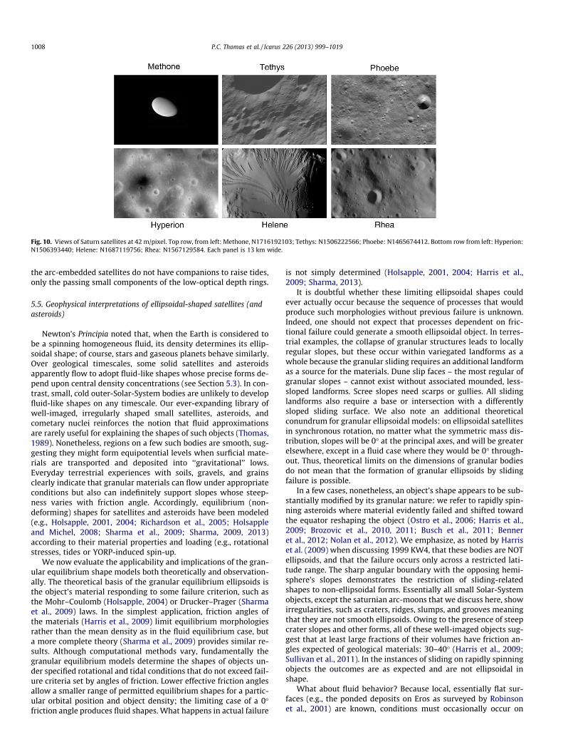
Fig. 10. Views of Saturn satellites at 42 m/pixel. Top row, from left: Methone, N1716192103; Tethys: N1506222566; Phoebe: N1465674412. Bottom row from left: Hyperion:N1506393440; Helene: N1687119756; Rhea: N1567129584. Each panel is 13 km wide.

1008 P.C. Thomas et al. / Icarus 226 (2013) 999–1019

the arc-embedded satellites do not have companions to raise tides,only the passing small components of the low-optical depth rings.

5.5. Geophysical interpretations of ellipsoidal-shaped satellites (andasteroids)

Newton’s Principia noted that, when the Earth is considered tobe a spinning homogeneous fluid, its density determines its ellip-soidal shape; of course, stars and gaseous planets behave similarly.Over geological timescales, some solid satellites and asteroidsapparently flow to adopt fluid-like shapes whose precise forms de-pend upon central density concentrations (see Section 5.3). In con-trast, small, cold outer-Solar-System bodies are unlikely to developfluid-like shapes on any timescale. Our ever-expanding library ofwell-imaged, irregularly shaped small satellites, asteroids, andcometary nuclei reinforces the notion that fluid approximationsare rarely useful for explaining the shapes of such objects (Thomas,1989). Nonetheless, regions on a few such bodies are smooth, sug-gesting they might form equipotential levels when surficial mate-rials are transported and deposited into ‘‘gravitational’’ lows.Everyday terrestrial experiences with soils, gravels, and grainsclearly indicate that granular materials can flow under appropriateconditions but also can indefinitely support slopes whose steep-ness varies with friction angle. Accordingly, equilibrium (non-deforming) shapes for satellites and asteroids have been modeled(e.g., Holsapple, 2001, 2004; Richardson et al., 2005; Holsappleand Michel, 2008; Sharma et al., 2009; Sharma, 2009, 2013)according to their material properties and loading (e.g., rotationalstresses, tides or YORP-induced spin-up.

We now evaluate the applicability and implications of the gran-ular equilibrium shape models both theoretically and observation-ally. The theoretical basis of the granular equilibrium ellipsoids isthe object’s material responding to some failure criterion, such asthe Mohr–Coulomb (Holsapple, 2004) or Drucker–Prager (Sharmaet al., 2009) laws. In the simplest application, friction angles ofthe materials (Harris et al., 2009) limit equilibrium morphologiesrather than the mean density as in the fluid equilibrium case, buta more complete theory (Sharma et al., 2009) provides similar re-sults. Although computational methods vary, fundamentally thegranular equilibrium models determine the shapes of objects un-der specified rotational and tidal conditions that do not exceed fail-ure criteria set by angles of friction. Lower effective friction anglesallow a smaller range of permitted equilibrium shapes for a partic-ular orbital position and object density; the limiting case of a 0�friction angle produces fluid shapes. What happens in actual failure

is not simply determined (Holsapple, 2001, 2004; Harris et al.,2009; Sharma, 2013).

It is doubtful whether these limiting ellipsoidal shapes couldever actually occur because the sequence of processes that wouldproduce such morphologies without previous failure is unknown.Indeed, one should not expect that processes dependent on fric-tional failure could generate a smooth ellipsoidal object. In terres-trial examples, the collapse of granular structures leads to locallyregular slopes, but these occur within variegated landforms as awhole because the granular sliding requires an additional landformas a source for the materials. Dune slip faces – the most regular ofgranular slopes – cannot exist without associated mounded, less-sloped landforms. Scree slopes need scarps or gullies. All slidinglandforms also require a base or intersection with a differentlysloped sliding surface. We also note an additional theoreticalconundrum for granular ellipsoidal models: on ellipsoidal satellitesin synchronous rotation, no matter what the symmetric mass dis-tribution, slopes will be 0� at the principal axes, and will be greaterelsewhere, except in a fluid case where they would be 0� through-out. Thus, theoretical limits on the dimensions of granular bodiesdo not mean that the formation of granular ellipsoids by slidingfailure is possible.

In a few cases, nonetheless, an object’s shape appears to be sub-stantially modified by its granular nature: we refer to rapidly spin-ning asteroids where material evidently failed and shifted towardthe equator reshaping the object (Ostro et al., 2006; Harris et al.,2009; Brozovic et al., 2010, 2011; Busch et al., 2011; Benneret al., 2012; Nolan et al., 2012). We emphasize, as noted by Harriset al. (2009) when discussing 1999 KW4, that these bodies are NOTellipsoids, and that the failure occurs only across a restricted lati-tude range. The sharp angular boundary with the opposing hemi-sphere’s slopes demonstrates the restriction of sliding-relatedshapes to non-ellipsoidal forms. Essentially all small Solar-Systemobjects, except the saturnian arc-moons that we discuss here, showirregularities, such as craters, ridges, slumps, and grooves meaningthat they are not smooth ellipsoids. Owing to the presence of steepcrater slopes and other forms, all of these well-imaged objects sug-gest that at least large fractions of their volumes have friction an-gles expected of geological materials: 30–40� (Harris et al., 2009;Sullivan et al., 2011). In the instances of sliding on rapidly spinningobjects the outcomes are as expected and are not ellipsoidal inshape.

What about fluid behavior? Because local, essentially flat sur-faces (e.g., the ponded deposits on Eros as surveyed by Robinsonet al., 2001) are known, conditions must occasionally occur on

Table 4Normal albedos on methone.

Evaluated at a = 5, i = 0

Leading side 0.618 ± 0.086 (0.024)Inner dark area 0.605 ± 0.040 (0.003)Dark oval 0.614 ± 0.081 (0.025)Bright surrounding 0.633 ± 0.086 (0.010)

Uncertainties listed include a contribution from extrapolating albedos to 5� phaseangle and a �5% absolute radiometric calibration uncertainty. Parentheses give 1rrelative errors.

P.C. Thomas et al. / Icarus 226 (2013) 999–1019 1009

small, airless objects wherein at least some regolith is fluidized.Asteroid Itokawa furnishes another example: smooth, low areas(slopes <1.2�; Barnouin-Jha et al., 2008) probably contain �cm-scale particles that should be able to sustain substantial staticslopes, but apparently have relaxed to an essentially level deposit.Distinctly filled craters are visible on Epimetheus (Fig. 1), suggest-ing the flow and segregation of a mobile regolith component thatwas emplaced just like a fluid. Similarly, material has drifted acrossDeimos’ surface despite slopes of only �2� (Thomas et al., 1996);this is geologically indistinguishable from fluid behavior. Yet thekey distinguishing element for Saturn’s arc-moons is the presenceof consistent properties or regolith dynamics over the entire visiblesurface such that the object maintains a smooth ellipsoidal form.Comparable, global-scale features have not been observed on anyother well-imaged small body. Landforms dominated by frictionalproperties are inherently variegated (note the example of 1999KW4, Fig. 3 in Ostro et al. (2006)). Absent indications that wholeobjects can be modified to approach an ideal failure envelope, forinterpretations of individual, specific smooth ellipsoids, it seemsmore fruitful presently to employ geophysical assumptions basedon fluid-like geological behavior. Such fluid-like behavior needonly extend to depths sufficient to flatten competing forms suchas crater rims and bowls.

5.6. The surface of Methone: photometry

Methone’s leading-hemisphere exhibits three conspicuous al-bedo features; a sharply-bounded, relatively dark oval centeredon the leading hemisphere, an even darker irregular splotch thatis centered almost exactly at the apex point on the body, and rela-tively bright material that surrounds the dark oval (Fig. 11a). Forthis photometric analysis we used the well-known Minnaert(1941) photometric model ((I/F) = B0 cosk(i)cosk�1(e) where B0 andk are the two model parameters to correct for incidence and emis-sion angles. Our best-fit Minnaert parameters for each image aregiven in Table S2; summary results are given in Table 4. To producethe albedo map, the photometrically corrected brightness valuesfrom each image were renormalized to represent normal albedosat (i = 0�, e = 5�, a = 5�) prior to map projection. We applied least-squared fits to the CL1–CL2 filter results giving B0 = �0.00396a + 0.6372 and k = �0.00309 a + 0.887 for the phase dependence

Fig. 11. Albedo and colors of Methone. (a) Broadband visible wavelength (611 nm) albedwas applied to each image for normalizing pixel-by-pixel values of albedo at a referencsimple-cylindrical map coordinates before merging and were contrast-stretched to sh0.61 ± 0.03, including the dark feathery feature near the center that has values as low asalbedo of 0.63 ± 0.01. For details, see Table 4. (b) (CL1:UV3)/(CL1:IR3) ratio of Methone(338 nm) and N1716192257 (930 nm).

of the Minnaert parameters. To optimize the spatial details, arealcoverage, and to reduce mapping artifacts, we combined map pan-els from the CL1–CL2 filter with the best-resolution images in theCL1–UV3, CL1–GRN, CL1–IR1, and CL1–IR3 filters. The brightness ofthe color-filter albedo images were adjusted to match those of theCL1–CL2 filter by applying the corresponding ratios from theMinnaert fits. An iterative approach was also applied to further ad-just the contrast levels in the color filter panels so that they best-matched those in the overlapping regions in the CL1–CL2 filterpanels. Following the approach summarized in Helfenstein et al.(1989), pixel-by-pixel weighted averaging was done to merge theindividual map panels into the composite map.

Normal albedos for the visible features are given in Table 4.Within the expected uncertainties, the average normal albedo ofthe visible leading-hemisphere (0.62 ± 0.09) is broadly consistentwith the geometric albedo of 0.57 ± 0.05 obtained from Methone’swhole-disk phase curve (see below). IR3/UV3 ratios show no trendwith albedo (Fig. 11b); the average IR3/UV3 ratio in all three albe-do divisions is 1.26. The absence of correlated patterns of color andalbedo on Methone suggests that the distinct albedo pattern is notthe result of systematic variations in surface composition. Rather,the patterns may arise from variations in some other surface phys-ical property, such as regolith grain size, soil compaction, or varia-tions in particle microstructure. Neither the contrast amounts, northe presence of a leading-side albedo marking are unusual for thismarking. What is distinctive is the sharp boundary, the precisecentering on the leading point, and the additional ‘‘swirl’’ featureat the leading point. It is not yet known whether similar patternsexist on the other arc-embedded satellites or the extent to whichthe pattern might exist but be obscured by surface relief on more

o map from the May 2012 Cassini flyby. A separate Minnaert photometric correctione incidence angle of 0� and phase angle of 5�. All of the images were projected toow subtle details. The prominent oval-shaped dark region has a mean albedo of0.60. The bright material surrounding the oval albedo boundary has a mean normalas a function of albedo from two Minnaert-corrected NAC images; N1716192136

Table 5Geometric albedos of embedded satellites from whole-disk phase curves (Hedmanet al., 2010).

Satellite Geometric albedo (611 nm)

Aegaeon 0.25 ± 0.23Methone 0.57 ± 0.05Anthe ?Pallene 0.47 ± 0.11

1010 P.C. Thomas et al. / Icarus 226 (2013) 999–1019

heavily cratered small satellites. However, the geography of the al-bedo pattern is suggestive of leading-side thermal anomalies thathave been identified on Mimas and Tethys (Howett et al., 2011,2012). The anomalies in those cases are believed to be producedby preferential bombardment of high-energy electrons on the lead-ing sides of those bodies. However, in those examples, the thermalanomalies coincide with a distinct decrease in IR/UV coloration,which is not detectable in our ISS high-resolution coverage ofMethone.

5.6.1. Albedos of arc embedded moonsHedman et al. (2010) obtained whole-disk, phase-curve mea-

surements of the embedded satellites from Cassini NAC CL1–CL2filter images at phase angles (10� < a < 60�) suitable for estimatingwhole-disk geometric albedos. However, Pallene was the only oneof the Alkyonide satellelites for which a reliable size estimate wasavailable, so that geometric albedos for Aegaeon, Anthe, and Meth-one could not be determined. Instead the phase curve data wereused to estimate the mean radii given the assumption that all ofthe satellites have the same geometric albedo as Pallene. Now,with our new size estimates (Table 1), we can use Hedmanet al.’s measurements to estimate the mean geometric albedos gi-ven in Table 5. As in Hedman et al. (2010), these values ignore theopposition effect and are extrapolated to zero phase. The error esti-mates include a 5% calibration uncertainty in absolute brightness(West et al., 2010) and a contribution from the size estimates in Ta-ble 1. It is also assumed that brightness variations due to Cassini’schanging viewing perspective average out over the phase curvemeasurements. While the error bars considerably overlap, the re-sults suggest that the geometric albedos may significantly varyamong the embedded satellites.

As yet, there are no reliable size determinations for Anthe. IfAnthe has the same geometric albedo as Pallene, then its meanradius would be about 1.1 km (Hedman et al., 2010). Our resultssuggest that the albedos of the satellites may significantly vary.We note that Hedman’s phase curve data was extrapolated froma phase angle range where the opposition surge can be neglected,so Anthe’s extrapolated geometric albedo should be no greaterthan unity, corresponding to a mean radius no less than about0.75 km. At the other extreme, if its geometric albedo is the sameas Aegaeon’s (pv = 0.25), then Anthe’s mean radius could be on theorder of 2.4 km, but could not be much larger because its size inour closest Cassini images would then be greater than a pixel(Table 1).

5.7. Ring/arc-embedded moons: summary

As smooth ellipsoids, the arc/ring embedded moons are uniqueamong well-imaged small Solar System bodies. The smooth surfaceof Methone suggests some mechanism of fluidizing the regolith ongeologic timescales. The mechanism is unknown, as the uniqueassociation with rings does not appear to provide an obvious routeto sufficiently rapid resurfacing to smooth impact craters. The den-sities inferred for these objects are low, but not grossly lower thansome directly measured values of small satellites and comet nuclei.Whether impacts into very porous regolith can enter a regime

where craters are much shallower than expected and ejecta subjectto global dispersal is not known, but might be one route to a geo-logically fluid outer region of the object. These distinctive objectsinvite work on the impact environment, ring/arc particle amountsand dynamics, the radiation environment, and small-satelliteaccretion studies.

6. Trojan satellites

Small satellites lie near the leading and trailing Lagrangianpoints of both Tethys (Telesto and Calypso) and Dione (Heleneand Polydeuces). Polydeuces is not well imaged (Table 1); Heleneis the best imaged among these at 42 m/pxl, over an object of meanradius of �18 km. The three well-imaged Trojan satellites all rotatesynchronously with their orbital periods as so far observed. TheHelene data are good enough (multiple observation times at suffi-cient resolution) to test for small forced librations. We detect nosuch rotational librations: the control point solutions have a min-imum in residuals consistent with no forced libration (Fig. S3).

For Calypso and Telesto, which have co-orbital libration ampli-tudes from 25% to 65% the size of Helene’s (Oberti and Vienne,2003; Murray et al., 2005), we obtained sufficiently precise resultsfrom a model assuming constant rotation rate. This result obtainsmainly because our high-quality observations have insufficienttemporal distribution to distinguish among different orientationmodels.

6.1. Shapes and surface features

Helene has only modest differences between its a and b axes(Table 1); Telesto and Calypso are much more elongated. The min-imum moment orientation calculated from the current shape mod-el of Helene is nearly 20� from the Saturn direction. Significanttopographic uncertainty remains in some unilluminated areas (atthe time of the last good coverage) in the north of Helene, whichmay contribute to this result. The slight difference in smallestand intermediate calculated moments means the orientations arenot tightly constrained, and thus no inference of inhomogeneityshould presently be inferred from the model moment orientationresults.

Helene, Calypso and Telesto have large craters, and have wide-spread filling of craters. Branching patterns of albedo and topogra-phy that are somewhat similar to drainage basins (Fig. 12) areevidence of long-range downslope transport. Such evidence oflong-range transport is absent on any of the other small saturniansatellites. The surface of a small body most similar to those of thesaturnian Trojan satellites is that of Deimos, which shows longrange transport over generally smooth surfaces without (exceptat its south pole) a pattern of collective ‘‘drainage.’’ Fig. 10 showsthat Helene (and by similar appearances the other Trojans) are dis-tinct from the more lunar-like small satellites and larger bodieswhose primary morphologic forms are crater-related.

6.2. High-resolution morphology of Helene

The high-resolution (<50 m/pixel) images of Helene show a sur-face with few visible sharp craters, some large, smoothed craters,and elongate, tapering darker surfaces that are higher than theirimmediate surroundings (Fig. 13). Here we designate these as the‘‘upper’’ (darker) and ‘‘lower’’ (lighter) units. The upper-surfaceexposures taper downslope and extend up to 8 km from high re-gions such as degraded large crater rims. The lower unit is brighter(especially in UV; see Section 6.4) and is in most places nearly fea-tureless at the highest resolutions. The darker, upper unit materialsform what appear to be residual mesas and pediment-like covers,

Fig. 12. Maps of Trojan satellites. Simple cylindrical projection. The upper three maps are stylized position plots of craters, the diameters are scaled to body mean radius.Calypso has outlines of the albedo markings added, and Telesto has the ‘‘drainage’’ pattern added. Bottom panel is a map of two UV3-CLR images of Helene high-pass filteredto show its ‘‘drainage pattern.’’.

P.C. Thomas et al. / Icarus 226 (2013) 999–1019 1011

Fig. 13. Best view of Helene. N1687119756, UV3 filter, phase = 97�, sub-spacecraftpoint is 2.7�N, 124.8�W. North is down in this presentation.

Fig. 14. Heights of scarps bounding upper surface from lower, smooth surface onHelene. Derived from shadow measurements. Error bars are derived by assuming a1.5 pixel error in shadow length. Abscissa is West longitude.

1012 P.C. Thomas et al. / Icarus 226 (2013) 999–1019

and show more fine topographic detail at 42+ m/pixel than doesthe lower unit. This kind of topography is clearly resolved in the re-gion 0–150�W, and is seen at �110 m/pixel in the region 150–250�W. In the 300–360�W range, observed at �230 m/pixel, theterrain may be rougher and have higher crater densities at 1–3 km diameter (Section 6.5; Fig. 17a, sub-Saturn vs. Leading side)and may hide thin tapered markings; however, we cannot confi-dently say whether the upper/lower units are present or absentin this region. The region 250–300�W is poorly observed.

This morphology suggests a covering, apparently widespread ifnot global, that has or is undergoing erosion at scarps and that issubject to long-distance downslope transport. Because the upperunit is thin, a characteristic immediately apparent from the modestshadow lengths and lack of expression on limb views, it is difficultto get accurate stereogrammetric measure of heights. The shapemodel of Helene is well enough constrained, however, to use sha-dow lengths to investigate the heights of the upper unit exposuresabove the adjacent lower unit. The results are shown in Fig. 14. Theaverage height of the scarps is 15.4 ± 12 m. Given the likely uncer-tainty in the individual measurements of <5 m, there is almost cer-tainly a real range of scarp heights; the vast majority are under20 m, and essentially all are under 30 m. These values are consis-tent with the inability to see any topography on the limb correlatingwith these forms (42 m/pixel or worse). The height of the scarpsmight be less than the height of the unit if the lower, smooth mate-rials were filling in around mesas of the upper materials. Given thelow slopes on the smooth materials (see Section 6.3), the presenceof scarps on topographic divides, and the long downslope extent ofroughly the same size and character of scarps, this morphologymost likely closely follows the thickness of an actual material unit.

The lower unit provides no thickness fiducials such as partiallyburied crater rims of known (expected) heights, or erosional expo-sures of a base. This layer covers large craters, most of which ap-pear far more degraded than anything attributable to a �20 mcover. The lower unit material thus is probably much thicker than

is the upper unit. For estimations of the amounts of materials beingmoved in this lower unit, we examine the crater densities on thedifferent units and parts of Helene in Section 6.5.

6.3. Comparison of the ‘‘drainage patterns’’ on the Trojan satellites

‘‘Drainage patterns’’ on the three Trojan satellites are comparedin Fig. 15. On Calypso the patterns of elongated light and darkmarkings are nearly hemispheric in extent; on Telesto they markrelatively smaller, more numerous ‘‘drainage basins’’. The taperingalbedo patterns on Calypso (observed at 130 m/pxl) are very simi-lar to those on Helene, and the high-resolution images of the latterare likely a key to both objects. There is some expression of topog-raphy in the elongated albedo patterns near the terminator on Ca-lypso, but these are not sufficiently resolved to obtain anythingother than crude estimates of relief. Telesto is seen at only mod-estly worse resolution than Helene (59 vs. 42 m/pxl) and doesnot replicate the distinct tapering pattern of markings seen on Ca-lypso and Helene. Telesto does clearly have a deep covering of deb-ris also subject to downslope motion, but with a more prominentconcentration in branching drainage patterns than on the otherTrojan satellites. Rims of the partially filled craters on Telesto arepreserved to the extent that blocks are still concentrated on therims. The material moving into and filling craters is not simplyrim material slumping into the craters. This material evidentlyhas much smaller particle sizes and is more widely dispersed thanthe near-rim ejecta.

Shape models are the basis for evaluating slopes and theamounts of materials in surface units. To calculate slopes, weneed a measure or estimate of the body mean density to evaluatethe sum of rotational and body-mass accelerations at the surface.We do not have direct mass measurements for these objects. Forslopes on Helene this is not a major problem because it has anorbital and rotational period of 2.74 days, so rotational accelera-tions are small relative to body gravity (rotational accelerationsat the sub-Saturn end are �0.0045 cm s�2). Calypso and Telestorotate more rapidly; they have 45-h periods that provide modestrotational accelerations, and thus might show more relative ef-fects of self-gravity and rotational acceleration. We have tested

Fig. 15. ‘‘Drainage’’ features on the Trojan satellites. Top row: Calypso drainage map locations; (see Fig. 2B) profiles calculated with mean density of 750 kg m�3; profilescalculated with mean density of 550 kg m�3. Second row: Telesto drainage map locations; profiles for mean density of 750 kg m�3. Slopes on the fill are 10–15�; profiles forassumed mean density of 500 kg m�3. Note the minimal difference in profiles for the two densities. Profile (1) includes two divides. Bottom row: Helene drainage maplocations; profiles, density used 750 kg m�3. Reference slope is 5�.

P.C. Thomas et al. / Icarus 226 (2013) 999–1019 1013

different mean densities for Calypso to see if its slopes are en-tirely downward along the apparent paths of motion of materialfor all densities, or if there is a density range where the slopewould be the wrong direction or would be interrupted in a man-ner not consistent with the image interpretation. This comparisonis limited by the nature of the smooth areas with elongatedmarkings: stereo solutions are widely spaced across the surfacebecause so few instances of local sharp contrast exist. The resultsfor three ‘‘drainage paths’’ on Calypso for mean densities of 550and 850 kg m�3 are shown in Fig. 15. The path traversing thegreatest longitude change (profile 1) is the most sensitive to rota-tional effects; the results are more plausible for the higher den-sity than for the lower because profiles 1 and 3 are morecontinuously sloped than for the lower density case. Because ofthe �100–150 m uncertainty in the topography along the profilesand possible ambiguities of where a drainage divide might bealong the linear markings that suggest flow, we conclude Calypsois probably more dense than the measured small saturnian satel-lites (Table 1), perhaps greater than 800 kg m�3. However, theconsiderable uncertainty of this estimate does not affect our con-clusion that a deep covering of loose material, likely ejecta, hasmoved downslope on these objects.

On Helene calculated slopes are not materially affected by theassumed mean density, and we may examine the character ofthe topography involved in downslope transport. Several pathsare plotted in Fig. 15. Slopes along these drainage paths are com-monly 6–9�. For comparison, significant downslope transport isobserved on 2� slopes on Deimos (Thomas et al., 1996) underroughly similar values of gravity (Deimos is smaller but probablydenser than Helene). Of course the materials, and some of the envi-ronment, are very different on the two objects.

On Telesto, calculated slopes along the main drainage paths are10–15� and approach 20� in some places (Fig. 15). The main drain-age paths on Telesto do not show diagnostic differences in topog-raphy as a function of assumed mean density (Fig. 15). The pathsare related to interior morphology of partly-filled/eroded craters,and to other low regions (�thalwegs) between topographic creststhat exhibit blocky forms that may be remnants of even largerhighly degraded impact craters.

Why are there drainage patterns on these satellites and nothingcomparable on other small satellites? More properly put, why arethere branching networks of slopes? Cratered landscapes havemany radial downslope motion forms, but paths through differentcraters requires some amount of erosion of rims and depositional

Fig. 16. Patterns of color on Helene and Calypso. Left: IR3/UV3 ratio image,stretched, of Helene images N1687120804 (IR3)/N1687120841 (UV3). Phaseangle = 64�; sub spacecraft point (average of pair) 1.5 N, 85.0�W. Upper unit,relatively dark in Fig. 13 (and in IR3 and CLR images) has a higher IR3/UV3 ratio; seeTable 6. See Fig. 13 for a UV3 image at higher phase angle. Right: stretched IR3/UV3ratio image of Calypso images N1644756439 (IR3)/N1644756637 (UV3). Phaseangle (average of pair) = 42.4�. For the Helene ratio image, due to its high-resolutionand complex shape, systematic changes in color with incidence and emission angleswere corrected by applying a separate, wavelength-dependent Minnaert photo-metric correction to each of the component color images (for IR3, B0 = 0.443,k = 0.74, and for UV3, B0 = 0.155, k = 0.76). These effects were not significant or wereotherwise confined to small areas of the Calypso ratio image.

1014 P.C. Thomas et al. / Icarus 226 (2013) 999–1019

smoothing to allow connections. The different amounts of inter-connected surfaces on the satellites range from the lunar-like cra-ter landscapes of Janus and Epimetheus, through the semi-globaldrainage patterns of the Trojans, to complete smoothing of thearc/ring embedded objects. Further work on the systematics ofcratering and ejecta motion in the inner Saturn system may eluci-date why the ‘‘drainage pattern’’ result is so unusual.

6.4. Color properties of Trojans and other small satellites

The tapered bright and dark markings on Helene and Calypso(and the less well-defined ones on Telesto) suggest some pro-cess-specific surface properties, and invite comparison of the col-ors to see whether the morphologic diversity is matched by colordiversity among the satellites (Morrison et al., 2010). Table 6 givesIR3/UV3 ratios for well-determined areas on several small satel-lites; this is a partial sampling of the data available for this work’spreliminary comparison among objects. Fig. 16 shows IR3/UV3 ra-tio images for Helene and for Calypso. The upper and lower surfacematerials on Helene are consistently different colors: the lowerunit has a IR3/UV3 value nearly 15% lower than that of the uppersurface. On Helene we can resolve the morphology and findunequivocally that surfaces with different geological processeshave different color properties. The colors on Telesto have a smal-ler range than do those on Helene. The IR/UV ratios on Calypso aresomewhat higher than those on Helene and have a spread of ratios(s.d. values in Table 6) more similar to those on Helene than onTelesto. Complications include viewing Helene and Calypso onleading sides (see Fig. 12), and the range of phase angles (Table 6).

The colors reported in Table 6 show the trend of bluer (or lessred) values moving away from the main rings as noted by Burattiet al. (2010) and Filacchione et al. (2010), due at least in part tothe influence of the E-ring particles. The process of E-ring particleimpacts (Verbiscer et al., 2007; Kempf et al., 2010) and chargedparticle bombardment (Johnson et al., 1985; Arridge et al., 2011;Howett et al., 2011, 2012) competes with geological processes,and on some satellites, especially Helene and Calypso, both leavestrong signatures. For Helene, the processes of erosion and down-slope motion result in a bluer surface; or a less active surface re-mains/becomes more red. Modeling of the interactions of smalland large impacts, charged particles, and the surface motion ofmaterials is left for future attempts to sort out rates of active pro-cesses in this system.

The IR3/UV3 color dichotomy is clearly defined on Helene. Forthe other satellites, local color-contrasts often define boundaries,sometimes distinct and sometimes diffuse or gradational, whereredder (high IR3/UV3) features transition to bluer (lower

Table 6IR3/UV3 color units for the small satellites.

Satellite IR3/UV3

Bluer Redder All

Ring shepherdsPrometheus 2.08 ± 0.14 2.41 ± 0.08 2.14 ±Pandora 1.84 ± 0.12 2.06 ± 0.05 1.85 ±

Co-orbitalsJanus 1.60 ± 0.05 1.73 ± 0.04 1.68 ±Epimetheus 1.69 ± 0.04 1.80 ± 0.05 1.76 ±

AlkyonidesMethone 1.26 ± 0.02 1.26 ± 0.03 1.26 ±

TrojansTelesto 1.04 ± 0.02 1.10 ± 0.02 1.06 ±Helene 1.05 ± 0.06 1.19 ± 0.04 1.09 ±Calypso 1.20 ± 0.04 1.29 ± 0.05 1.23 ±

1.26 ± 0.05 1.36 ± 0.04 1.32 ±

IR3/UV3) ones. On the other satellites we distinguished the colorunits by incrementally DN-slicing the color ratio images into twocolor units that best match the spatial pattern of coherent redderand bluer units, respectively. In the separate analysis of Methone(see Section 5.5), the units were defined a priori by the segregationof materials shown in the albedo map (Fig. 11). In all other cases,the color units are defined exclusively by the ratio images andare independent of albedo patterns seen in the corresponding ori-ginal images from which they were constructed. Consequently, anycorrelation of color unit with albedo is an independent result.

On Helene, Calypso, and Pandora, the spatial distribution of col-or units is strongly correlated with albedo features: redder materi-als tend to be darker, and bluer materials tend to be brighter. Forthe remaining satellites the relationship is less well-defined orindeterminate. In the case of Epimetheus and Methone the rangeof visible albedos is very small. In our Epimetheus images the smallalbedo variations can be easily muted by brightness variations dueto surface relief. On Janus and Telesto the relationships are non-un-ique and examples can be found where redder units correspond tolocally brighter materials, in addition to the expected relationship

Phase angle (�) Images used IR3: UV3

0.18 31 N1640497881: N16404979270.13 54 N1504612418: N1504612385

0.08 58 N1627323305: N16273232270.07 65 N1575363199: N1575363109

0.02 61 N1716192257: N1716192136

0.04 58 N1514163666: N15141636000.09 64 N1687120804: N16871208410.07 42 N1644756637: N16447564390.07 91 N1644754794: N1644754596

P.C. Thomas et al. / Icarus 226 (2013) 999–1019 1015

in other regions. In many instances imperfections in the shapemodel can introduce artifacts that mimic albedo patterns in photo-metrically corrected albedo images. Unresolved differences in sub-pixel-scale surface relief or roughness can also produce artifactsthat appear as dark albedo patches when illuminated at moderateto high incidence angles. However, in some examples, the inversecolor-albedo relationship appears to be real, particularly in a fewcases where bright crater ejecta correspond to redder material.We may conclude that the colors of small satellite features areprobably not uniquely tied to their stratigraphic age.

6.5. Crater densities on Trojans and other small satellites

We use relative (R-plot) and cumulative number/area analysisto compare crater densities (Crater Analysis Working Group1979). The primary obstacle in crater density analysis on irregu-larly-shaped objects is the variety of viewing conditions imposedby the different flyby conditions: typically less than one-third thesurface is well observed at the closest point of an encounter. Com-parisons between objects must allow for different viewing and res-olutions. However, there are enough data on several of theseobjects for revealing comparisons.

Fig. 17. Crater densities on small saturnian satellites: relative (top panels) and cumulatiand lower units, and for the entire area (�0–150�W) imaged at high resolution (42–60 mp

n. (b) Crater densities on Trojan satellites: leading side of Helene, composites of Calyps(c) Crater densities on Helene and composite curves for other small saturnian satellites.

Helene is sufficiently well resolved in the best encounter to giveinformation on crater densities on the upper and lower units overnearly a hemisphere. Fig. 17a shows crater densities for differentsections of Helene: the best viewed region (0–150�W) at42–60 m/pixel, which includes the upper surface and lower surfaceunits, a global count of craters with diameters J 2 km and a sec-tion of Helene, between longitudes 310–360�W (labeled ‘‘sub-Sat-urn’’), that is seen sufficiently well to count craters >1 km. Thelarger craters are included in the regional tabulations, but are notincluded in the two unit counts as both units appear to superposethe large craters.

The combination of R and cumulative plots yield three conclu-sions. 1: The crater densities superposed on the upper and lowersurfaces are indistinguishable from each other, although limitedin size range of data. We cannot distinguish ages or crater-reten-tion properties of these units. Because the upper surface may beless disturbed than the lower one which has undergone (or isundergoing) active transport, it conceivably could show a highercrater density, but we cannot really test this possibility becauseof the small numbers of craters involved. 2: The regional and globaltabulations show the fall-off of relative crater densities typical ofsaturnian satellites at diameters less than �10 km (Richardson

ve (lower panels) densities. (a) Regions on Helene: densities of craters on the upper/pixel), sub-Saturn region 300–360�W imaged at 230 m/pixel. Error bars are simplyo and Telesto that include best imaged areas and global coverage for largest craters.

Table 7Estimated crater fill on Telesto.

Diam. Depth Dimensions, km Fill Average fill

Nominal depth Max.

Dimensions, km6.4 0.6 1–1.3 0.4 0.7 0.13–0.238.9 0.5 1.3–1.8 0.8 1.3 0.26–0.437.1 0.4 1.1–1.4 0.7 1.0 0.23–0.33

Nominal depth with d/D of 0.15–0.20.

1016 P.C. Thomas et al. / Icarus 226 (2013) 999–1019

and Thomas, 2010). This has been attributed largely to the impac-tor size distribution (Richardson and Thomas, 2010). 3: There arereal and substantial differences in crater density across the surfaceof Helene at least at diameters between 0.5 and 3 km.

We now examine point 3 in more detail. The leading side datataken alone have the R-plot fall-off and S-curve shaped cumulativeplot that might indicate an impactor size distribution, or a two-stage history where smaller craters were largely obliterated andare now recovering their density. This latter scenario has been acommon interpretation on many surfaces and likely is correct inmany instances. The sub-Saturn and leading sides have distinctlydifferent densities of craters from 1 to 3 km diameter, and the sub-set of the leading side in the upper and lower units is distinct fromthe leading side totals from 0.5 to 0.8 km. No single crater popula-tion or episode can cover all three curves. While the leading sidecurve by itself might indicate one population interrupted by ero-sion, the difference between the subset of that population andthe size distribution in the sub-Saturn area indicates that the samescenario cannot apply to the whole object. Either different areashave different surface processes modifying the crater populations,or areas of different ages were subject to different impactingpopulations. We cannot choose between these scenarios with thecurrent data.

A comparison of crater densities on the three Trojans is shownin Fig. 17b. The data are from the best viewed portions of all threeobjects. There is a suggestion that near 1 km diameter Calypso ismore densely cratered than Helene, but the large uncertaintiesfrom the small number counted means this is only a possibility.

In Fig. 17c, The Helene data are compared to several other smallsaturnian satellites; the variation shown in Fig. 17b should be keptin mind viewing this plot. Between 1 and 10 km there is somespread of the data with Helene being the most heavily cratered,and Prometheus the least, but differences are marginally signifi-cant. Only Phoebe stands out at small sizes, below 700 m diameter,and it is compositionally and orbitally distinct from the other ob-jects that we consider.

6.6. Depths of materials inferred on Helene, Calypso and Telesto

The crater density data do not allow a clear determination thatcertain sizes of craters on the Trojan satellites have been removedby covering and burial. We thus estimate covering by measure-ments of dimensions of discrete fill in craters, and by a fewdepth/diameter measurements.

6.6.1. Discrete fill deposits visible in cratersDegraded craters with definable amounts of filling by the lower

unit material help to give estimates of local thicknesses of craterfill on Helene. A 5.6 km crater (�12�, 70�W) has a smooth fill3.6 km in diameter. If we approximate the crater as a paraboloidof revolution, with height h = 0.15D or 0.3r, the volume is(p/2) � ha2 or 0.059D3. The relative volume of the fill is simply(Df/Dc)3, or 0.25. The volume of the crater is modeled as10.9 km3, the fill 2.7 km3. This fill is assumed to have been gath-ered from the crater’s 25.5 km2, for a model average depth of0.11 km. Similarly, a 9.8 km crater (�37�, 174�W) has a flat deposit3.6 km in diameter, which we model as 2.75 km3 derived from75.4 km2, or an average depth of 0.036 km.

6.6.2. Depths of large cratersWe may take the depths of some of the large craters on Helene

without discrete fill margins and test if their depths have been re-duced by filling. This approach is limited by our relative ignoranceof the expected fresh crater depth, and effects of modifications tothe crater morphology other than simple filling. There arefour well-measured craters with covering by the lower unit

11.5–15 km in diameter in the well-imaged area. These havedepth/diameter ratios of 0.12, 0.16, 0.17, and 0.036. Fresh craterson these objects are probably �0.15D in depth, although this is apoorly determined ratio for small body craters (Carr et al., 1994;Sullivan et al., 1996; Besse et al., 2012). We simply assume thatthe three deepest, being close to an expected value of �0.15 fordepth/diameter, are little affected by filling. We assume the othercrater, 11.5 km in diameter and 410 m in depth, has filled froman original depth of 0.15 � 11.5 km or 1.73 km. The difference involume, obtained by modeling the crater and subtracting the nom-inal and modified volumes, is 26 km3. This material is assumed tohave been gathered over the crater’s 104 km2 area, implying anaverage fill depth of 0.25 km.

6.6.3. Overall estimates for cover on TrojansIn summary, our estimates of the covering on Helene which is

the combination of the upper and lower units, include 40–110 mcalculated from discrete fill deposit geometry, and up to 250 m cal-culated from one large crater depth. The discrete fill data are prob-ably the best measurement among these as it is the most directobservation with the fewest assumptions. Thus we make an overallestimate of 40–180 m of cover. This material post-dates most ofthe 2+ km diameter craters.

On Telesto, a few crater depths may be estimated from stereoand shadows. The estimated average fill depth within these cratersis 0.13–0.43 km (Table 7). For Calypso, the covering does not allowestimates of fill within specific craters, and we do not know thesize of features that are buried by the widespread debris covering.The topography above the smoother, lineated materials is >200 m,the maximum depths of burial could be greater than this value, butwe have no way to restrict these depths.

6.6.4. Predicted ejecta volumesThe role of crater ejecta in any self-covering of these objects de-

pends upon the number of craters and their volumes, the initialdistribution of ejecta (whether it lands close to craters or goes intoSaturn orbit and is subsequently reaccumulated), and the timingfor formation of large craters supplying ejecta relative to formationtimes of craters or other topography being buried. We can take thevisible crater population and estimate ejecta volumes, but we mustbe aware that the covering and erosion themselves make this aminimum estimate that needs additional context. We take the glo-bal crater densities (actually, the most nearly global compilationsscaled for the fractional area involved) and simply apply the aboveapproximation of crater volume of V = 0.059D3 (on the low-gravityobjects, all craters should be simple) to obtain estimates given inTable 8.

Any two of the four largest craters on Helene could supply a glo-bal covering of �50 m. In the high-resolution images the upper andlower units post-date the larger craters, but there are large cratersseen at longitudes outside the 0–150�W range of the high-resolution coverage that could supply this amount of material,but because of much lower resolution, the stratigraphic relationof the craters in this region to the covering cannot be established.

Table 8Predicted ejecta on selected satellites.

Object Total area, (km2) Count area (km2) Vol. (km3) Depth (km) Depth (Rm)

Helene 4380 3810 1140 0.30 0.017Calypso 1310 910 87 0.10 0.01Telesto 2075 1600 310 0.19 0.016Janus 104090 99540 50020 0.50 0.006Epimetheus 44760 42570 11800a 0.28 0.005

61600 1.45 0.025Phoebe 147000 147000 241000 1.7 0.016

a Value excludes south polar depression.

P.C. Thomas et al. / Icarus 226 (2013) 999–1019 1017

Although we cannot rule out Helene being self-covered, the dis-tinct appearance of these covering units on Helene and Calypsosuggests different processes or histories from the large-scale cra-tering, covering, and gardening seen on other well-imaged objects.Additionally, the geographical variation in crater densities(Section 6.5) on Helene suggests effects other than build-up of ran-domly distributed cratering.

For comparison, the satellite best known for a nearly global,smooth covering by likely ejecta is Deimos. The latter object mayhave achieved its appearance from an �80 m cover of ejecta com-ing from a single, large crater. The estimated ejecta depth over this6 km radius object is only 0.013Rm, on the order of those values inTable 8. The south polar 94 km depression on Epimetheus, ifcounted as a crater, completely dominates the calculated ejecta(Table 8), yet the surface within that crater is old enough to haveaccumulated a large population of craters. Deimos’s large crater(�7.5 km diameter) is young enough that only a modestpopulation of superposed craters exists, in addition to some cratersapparently buried and re-exposed by downslope motion of theaccumulated ejecta (Thomas, 1998). Deimos’s radically differentappearance from that of Epimetheus may arise simply because ofthe different relative timing of the largest cratering events.1

6.7. Interpretations of surfaces of Trojan satellites

While we cannot rule out craters on Helene providing its cover-ing materials, global distribution of ejecta is not what is expected.The dominance of gravity scaling of craters even on small (butweak) objects (Asphaug and Melosh, 1993; Richardson, 2009)should leave most ejecta concentrated near the source crater. Thedetailed information available on the martian satellites supportsthe prediction (Thomas, 1998) that most ejecta landed nearlarge source craters: both near Stickney (D = 9.4 km; PhobosRm = 11.1 km) on Phobos and near the unnamed �9 km crater onDeimos (Rm = 6.2 km). Both require large radial variations in ejectathicknesses. The upper layer on Helene (Fig. 14) shows no orga-nized pattern in thickness. Initial truly global distribution of ejectaon Helene (really escaped and recaptured ejecta) would probablyrequire very high-strength materials that foster higher velocityejecta than would be generated by cratering in a largely gravity-scaling environment. The high inferred porosities of these objectsis an indication that high-strength materials do not have a role incratering on these bodies.

Apart from material properties, the distinction of the Trojan sa-tellite appearances may be the dynamical position. The dynamicalpositions could be important if the associated large satellites,Tethys and Dione, could supply materials for accretion onto theTrojans that are not available to satellites such as Janus, Epime-theus, Phoebe or others. This scenario of course requires escapeof ejecta from a much deeper gravity well than the Trojans have.The offsetting factor would be the relative areas of Tethys andDione compared to the Trojans and the very large craters thatcan occur on those surfaces. Dione has �900 times the area of

Helene, so a 100 m cover on Helene would correspond to the vol-ume of an 11 cm cover on Dione. Tethys has �2700 times the areaof Calypso, so a 100 m layer on Calypso is equivalent to a �37 cmcover on Tethys. For Helene the required volume is �200–800 km3

(40–180 m over an area of 4390 km2 from the shape model).Exchange of ejecta among satellites in the Saturn system and

specifically Tethys and its Trojans has been modeled by Alvarelloset al. (2005) and Dobrovolskis et al. (2009). Large impacts intoTethys such as Odysseus (440 km diameter, leading side) andPenelope (180 km diameter, trailing side) were taken as sourcesof ejecta. Although a large fraction of the escaping material couldin principle reach the Lagrangian points, only 0.1% intersects thesmall cross sections of these moons. The simulations did not in-clude oblique impacts, jetting, or radiative or magnetospheric ef-fects on small particles. Because escaping, high-velocity ejectawill assume semi major axes different from the source body, ejectafrom Tethys can reach Enceladus and Dione. Thus, it might be ex-pected that covering on Tethys’s Trojans might have a significantcomponent originating from Dione, and Helene might acquire deb-ris from Tethys. Both Dione and Tethys have at least five craters>100 km diameter, with ejecta volumes >15,000 km3 each, assum-ing 2 km of excavation. We conclude that more specific modelingof the large crater histories on Tethys and Dione are needed to testwhether there would be enough ejecta in their orbits for a long en-ough time for the Trojans to pick up sufficient ejecta from the out-side to distinguish their appearance from other small satellites thatdo not share orbits with much larger objects that might be sourcesof external ejecta.

7. Overall properties of the small satellites

Albedo and colors of the small satellites show trends with dis-tance from Saturn, and surface morphology varies with dynamicalposition. The mean densities also show a radial trend (Fig. 18a), butone that would appear to peak with the co-orbitals. However, theirdensities as a function of mean radius, thus as something of a func-tion of internal pressures, also show some correlation (Fig. 18b).The central pressures in all of these objects are low compared tothe medium-sized moons where compaction might play some role(Eluszkiewicz, 1990). On such low-density, low-pressure objects,dynamical pressures associated with impacts might be suspectedof a role in determining porosities, but the smooth surfaces ofMethone and Pallene make such speculation dubious. Modelingof the evolution of all these bodies is at an early stage, but Cassinihas now provided more constraints on such inquiries.

8. Summary

The surface features of the inner small satellites of Saturn arespecific to the dynamical environment each satellite occupies(Table 9). Satellites within the main rings, embedded within ringarcs, or in Trojan orbits display a variety of depositional modifica-tions. The F-ring shepherds and the co-orbitals display more

Table 9Morphologic characteristics of Saturn inner small satellites.

Within mainrings

Pan Equatorial ridge

Daphnis Equatorial ridge?Atlas Equatorial ridge

F-ringshepherds

Prometheus Stripped core? Cratered

Pandora Cratered, grooves

Co-orbital Epimetheus Cratered, groovesJanus Cratered

Arc, diffusering

Aegaeon Ellipsoid

Methone Smooth ellipsoidAnthe ?Pallene Smooth ellipsoid

Trojan Telesto Deep crater fill, downslope transportCalypso Deep fill, global downslope transportPolydeuces ?Helene Global deposition, backwasting, downslope

transport

Fig. 18. Mean density of inner small satellites. (a) As function of distance fromSaturn. (b) As function of satellite mean radius.

1018 P.C. Thomas et al. / Icarus 226 (2013) 999–1019

heavily cratered surfaces, more evidence of internal structural fea-tures, and minimal depositional materials. The arc-embeddedmoons are likely near-equilibrium forms and have low densities,with implied porosities reaching �65%. The combination of surfacefeatures correlated with dynamical position, and the presence of

significant depositional forms, suggests ongoing processes in theinner Saturn system able to compete with cratering modificationsof surfaces. We confirm that photometric and color properties formany of these small satellites are dependent on distance from Sat-urn. From Atlas to the Trojans albedos generally increase and col-ors become bluer (Buratti et al., 2010) likely showing theinfluence of E-ring particles, whose eventual source is Enceladus(Verbiscer et al., 2007). Spectrally these satellite surfaces all appearto be water ice with minimal contaminants that are distinct fromthose in the darker components of regoliths of outer satellites suchas Iapetus, Phoebe or Hyperion (Buratti et al., 2010; Filacchioneet al., 2010). Although albedo and colors show radial trends fromSaturn, local geology, such as downslope transport, also affects col-or properties and may indicate relative rates of different processes.

One of the primary lessons of this study is how little we know ofthe processes that move material around on low-gravity surfaces.We do not know how arc/ring embedded moons are smoothed,nor if they relate to smoothing on objects such as Atlas. We donot know how the ‘‘drainage basin’’ patterns on the Trojan moonsare established and modified. We do not know how the sharp albe-do boundary on Methone is generated or maintained. In short, elu-cidating the competing regolith processes on these bodies hasbarely started.

Acknowledgments

Funded in part by the Cassini Project. We thank T. Ansty, B.Carcich, K. Consroe, T. Denk, R. Rich Goldweber, C. Jackman,J. Joseph, T. Shannon, P. Smith, D. Wilcox for technical help.Reviews by J. Spitale and an anonymous reviewer helpedstrengthen the paper’s presentation.

Appendix A. Supplementary material

Supplementary data associated with this article can be found, inthe online version, at http://dx.doi.org/10.1016/j.icarus.2013.07.022.

References

Alvarellos, J.L., Zahnle, K.J., Dobrovolskis, A.R., Hamill, P., 2005. Fates of satelliteejecta in the Saturn system. Icarus 178, 104–123.

Archinal, B.A. et al., 2011. Report of the IAU working group on cartographiccoordinates and rotational elements: 2009. Celest. Mech. Dyn. Astron. 109, 101–135.

Arridge, C.S. et al., 2011. Mapping magnetospheric equatorial regions at Saturn fromCassini Prime Mission Observations. Space Sci. Rev. 164, 1–83.

Asphaug, E., Melosh, H.J., 1993. The Stickney impact of Phobos - A dynamical model.Icarus 101, 144–164.

Barnouin-Jha et al., 2008. Small-scale topography of 25143 Itokawa from theHayabusa laser altimeter. Icarus 198, 108–124.

Benner, L.A.M. et al., 2012. Arecibo and goldstone radar observations of binary near-Earth asteroid and marco Polo-R Mission Target (175706) 1996 FG3. AAS/Division for Planetary Sciences Meeting 44. Abstracts #102.06.

Besse, S., Lamy, P., Jorda, L., Marchi, S., Barbieri, C., 2012. Identification and physicalproperties of craters on Asteroid (2867) Steins. Icarus 221, 1119–1129.

Brownlee, D.E. et al., 2004. The surface of young Jupiter family Comet Wild 2: Viewfrom the Stardust spacecraft. Science 304, 1764–1769.

Brozovic, M. et al., 2010. Radar images and shape model of a triple Asteroid(136617) 1994CC. Bull. Am. Astron. Soc. 42, 1080.

Brozovic, M. et al., 2011. Radar and optical observations and physical modeling oftriple near-Earth Asteroid (136617) 1994 CC. Icarus 216, 241–256.

Buratti, B.J. et al., 2010. Cassini spectra and photometry 0.25–5.1 lm of the smallinner satellites of Saturn. Icarus 206, 524–536.

Burns, J.A. et al., 2004. Jupiter’s ring-moon system. In: Bagenal, F., Diwling, T.E.,McKinnon, W.B. (Eds.), Jupiter: The Planet, Satellites, and Magnetosphere.Cambridge Univ. Press, pp. 241–262.

Busch, M.W. et al., 2011. Radar observations and the shape of near-Earth Asteroid2008 EV5. Icarus 212, 649–660.

Carr, M.H., Kirk, R.L., McEwen, A., Veverka, J., Thomas, P., Head, J.W., Murchie, S.,1994. The geology of Gaspra. Icarus 107, 61–71.

P.C. Thomas et al. / Icarus 226 (2013) 999–1019 1019

Castillo-Rogez, J.C., Johnson, T.V., Thomas, P.C., Choukroun, M., Matson, D.L., Lunine,J.I., 2012. Geophysical evolution of Saturn’s satellite Phoebe, a largeplanetesimal in the outer Solar System. Icarus 219, 86–109.

Chandrasekhar, S., 1969. Ellipsoidal Figures of Equilibrium. Yale Univ. Press, NewHaven.

Charnoz, S., Brahic, A., Thomas, P.C., Porco, C.C., 2007. The equatorial ridges of Panand Atlas: Terminal accretionary ornaments? Science 318, 1622–1624.

Denk, T., Mottola, S., Roatsch, T., Rosenberg, H., Neukum, G., 2011. Rotation periodsof irregular satellites of Saturn. EPSC-DPS Joint Meet. Abstract #1452.

Dermott, S.F., 1979. Shapes and gravitational moments of satellites and asteroids.Icarus 37, 575–586.

Dermott, S.F., Murray, C.D., 1981a. The dynamics of tadpole and horseshoe orbits. I –Theory. Icarus 48, 1–11.

Dermott, S.F., Murray, C.D., 1981b. The dynamics of tadpole and horseshoe orbits II.The coorbital satellites of Saturn. Icarus 48, 12–22.

Dermott, S.F., Thomas, P.C., 1988. The shape and internal structure of Mimas. Icarus73, 25–65.

Dobrovolskis, A.R., Burns, J.A., 1980. Life near the Roche limit – Behavior of ejectafrom satellites close to planets. Icarus 42, 422–441.

Dobrovolskis, A.R., Alvarellos, J.L., Zahnle, K.J., Lissauer, J.J., 2009. Fates of ejecta fromco-orbital satellites: Tethys, Telesto, and Calypso. AGU (Fall Meet.). Abstracts1146.

Dones, L., Chapman, C.R., McKinnon, W.B., 2009. Icy satellites of Saturn: Impactcratering and age determination. In: Saturn from Cassini–Hyugens. Springer, pp.613–635.

Eluszkiewicz, J., 1990. Compaction and internal structure of Mimas. Icarus 84, 215–225.

Filacchione, G. et al., 2010. Saturn’s icy satellites investigated by Cassini–VIMS. II.Results at the end of nominal mission. Icarus 206, 507–523.

Fujiwara, A. et al., 2006. The rubble-pile Asteroid Itokawa as observed by Hayabusa.Science 312, 1330–1334.

Gladman, B. et al., 2001. Discovery of 12 satellites of Saturn exhibiting orbitalclustering. Nature 412, 163–166.

Harris, A.W., Fahnestock, E.G., Pravec, P., 2009. On the shapes and spins of ‘‘rubblepile’’ asteroids. Icarus 199, 310–318.

Hedman, M.M. et al., 2007. The source of Saturn’s G ring. Science 317, 653–656.Hedman, M.M., Murray, C.D., Cooper, N.J., Tiscareno, M.S., Beurle, K., Evans, M.W.,

Burns, J.A., 2009. Three tenuous rings/arcs for three tiny moons. Icarus 199,378–386.

Hedman, M.M., Cooper, L.J., Murray, C.D., Beurle, K., Evans, M.W., Tiscareno, M.S.,Burns, J.A., 2010. Aegaeon (Saturn LIII), a G-ring object. Icarus 207, 433–447.

Helfenstein, P., Hillier, J., Veverka, J., Moersch, J., Weitz, C., 1989. Uranus satellites:Albedo and color maps from Voyager imaging. Lunar Planet. Sci. 20, 402–403(abstract).

Helfenstein, P. et al., 1994. Galileo photometry of Asteroid 951 Gaspra. Icarus 107,37–60.

Hirata, N., Miyamoto, H., 2012. Dust levitation as a major resurfacing process on thesurface of a saturnian icy satellite, Atlas. Icarus 220, 106–113.

Holsapple, K.A., 2001. Equilibrium configurations of solid cohesionless bodies.Icarus 154, 432–448.

Holsapple, K.A., 2004. Equilibrium figures of spinning bodies with self-gravity.Icarus 172, 272–303.

Holsapple, K.A., Michel, P., 2008. Tidal disruptions. II. A continuum theory for solidbodies with strength, with applications to the Solar System. Icarus 193, 283–301.

Howard, A.D., Moore, J.M., Schenk, P.M., White, O.L., Spencer, J., 2012. Sublimation-driven erosion on Hyperion: Topographic analysis and landform simulationmodel tests. Icarus 220, 268–276.

Howett, C., Spencer, J.R.J., Schenk, P., Johnson, R.E., Paranicas, C., Hurford, T.,Verbiscer, A., Segura, M., 2011. A high-amplitude thermal inertia anomaly ofprobable magnetospheric origin on Saturn’s moon Mimas. Icarus 216, 221–226.

Howett, C.J.A., Spencer, J.R., Hurford, T., Verbiscer, A., Segura, M., 2012. PacManreturns: An electron-generated thermal anomaly on Tethys. Icarus 221, 1084–1088.

Jacobson, R.A. et al., 2006. The gravitational field of Saturn and the masses of itsmajor satellites. Astron. J. 132, 2520–2526.

Jacobson, R.A. et al., 2008. Revised orbits of Saturn’s small inner satellites. Astron. J.135, 261–263.

Johnson, R.E. et al., 1985. Charged particle modification of ices in the saturnian andjovian systems (in ices in the Solar System). NATO ASI Ser. 156, 301–315.

Johnson, T.V., Castillo-Rogez, J.C., Matson, D.L., Thomas, P.C., 2009. Phoebe’s shape:Possible constraints on internal structure and origin. Lunar Planet. Sci. 40.Abstract #2334.

Keller, H.U. et al., 2010. E-type Asteroid (2867) Steins as imaged by OSIRIS on boardRosetta. Science 327, 190–193.

Kempf, S., Beckmann, U., Schmidt, J., 2010. How the Enceladus dust plume feedsSaturn’s E ring. Icarus 206, 446–457.

Minnaert, M., 1941. The reciprocity principle of linear photometry. Astrophys. J. 93,403–410.

Morrison, S.J., Thomas, P.C., Tiscareno, M.S., Burns, J.A., Veverka, J., 2009. Grooves onsmall saturnian satellites and other objects: Characteristics and significance.Icarus 204, 262–270.

Morrison, S.J., Helfenstein, P., Thomas, P.C., Veverka, J., 2010. Color photometry ofthe small saturnian satellites: Global and regional variations on Prometheusand Calypso. Bull. Am. Astron. Soc. 42, 955.

Murray, C.D., Cooper, N.J., Evans, M.W., Beurle, K., 2005. S/2004 S5: A new co-orbitalcompanion for Dione. Icarus 179, 222–234.

Nolan, M.C. et al., 2012. The shape of OSIRIS-REx mission target 1999 RQ36 fromradar and lightcurve data. LPI Contrib. 1667, 6345.

Noyelles, B., 2010. Theory of the rotation of Janus and Epimetheus. Icarus 207, 887–902.

Oberti, P., Vienne, A., 2003. An upgraded theory for Helene, Telesto, and Calypso.Astron. Astrophys. 397, 353–359.

Ostro, S.J. et al., 2006. Radar imaging of binary near-Earth Asteroid (66391) 1999KW4. Science 314, 1276–1280.

Owen Jr., W.M., 2003. Cassini ISS geometric calibration. JPL InterofficeMemorandum 312 (E-2003-001).

Porco, C.C. et al., 2004. Cassini Imaging Science: Instrument characteristics andanticipated scientific investigations at Saturn. Space Sci. Rev. 115, 363–497.

Porco, C.C. et al., 2005. Cassini Imaging Science: Initial results on Phoebe andIapetus. Science 307, 1237–1242.

Porco, C.C., Thomas, P.C., Weiss, J.W., Richardson, D.C., 2007. Saturn’s small innersatellites: Clues to their origins. Science 318, 1602–1607.

Richardson, J.E., 2009. Cratering saturation and equilibrium: A new model looks atan old problem. Icarus 204, 697–715.

Richardson, J.E., Melosh, H.J., 2013. An examination of the Deep Impact collision siteon Comet Tempel 1 via Stardust-NExT: Placing further constraints on cometarysurface properties. Icarus 222, 492–501.

Richardson, J.E., Thomas, P.C., 2010. Uncovering the saturnian impactor populationvia small satellite cratering records. Lunar Planet. Sci. 41. Abstracts 1523.

Richardson, D.C., Elankumaran, C.P., Sanderson, R.E., 2005. Numerical experimentswith rubble piles: Equilibrium shapes and spins. Icarus 173, 349–361.

Robinson, M.S., Thomas, P.C., Veverka, J., Murchie, S., Carcich, B., 2001. The nature ofponded deposits on Eros. Nature 413, 396–400.

Robutel, P., Rambaux, N., Castillo-Rogez, J., 2011a. Analytical description of physicallibrations of saturnian coorbital satellites Janus and Epimetheus. Icarus 211,758–769.

Robutel, P., Rambaux, N., El Moutamid, M., 2011. Influence of the coorbitalresonance on the rotation of the Trojan satellites of Saturn. arXiv:1111.1076(e-prints).

Roussos, E. et al., 2008. Energetic electron signatures of Saturn’s smaller moons:Evidence of an arc of material at Methone. Icarus 193, 455–464.

Russell, C.T. et al., 2012. Dawn at Vesta: Testing the protoplanetary paradigm.Science 336, 684–686.

Sharma, I., 2009. The equilibrium of rubble-pile satellites: The Darwin and Rocheellipsoids for gravitationally held granular aggregates. Icarus 200, 636–654.

Sharma, I., 2013. Structural stability of rubble-pile asteroids. Icarus 223, 367–382.Sharma, I., Jenkins, J.T., Burns, J.A., 2009. Dynamical passage to approximate

equilibrium shapes for spinning, gravitating rubble asteroids. Icarus 200, 304–322.

Simonelli, D.P., Thomas, P.C., Carcich, B.T., Veverka, J., 1993. The generation and useof numerical shape models for irregular Solar System objects. Icarus 103, 49–61.

Sullivan, R. et al., 1996. Geology of 243 Ida. Icarus 120, 119–139.Sullivan, R., Anderson, R., Biesiadecki, J., Bond, T., Stewart, H., 2011. Cohesions,

friction angles, and other physical properties of martian regolith from MarsExploration Rover wheel trenches and wheel scuffs. J. Geophys. Res. (Planets)116, 2006. http://dx.doi.org/10.1029/2010JE003625.

Thomas, P., 1989. Shapes of small satellites. Icarus 77, 248–274.Thomas, P.C., 1993. Gravity, tides, and topography on small satellites and asteroids

– Application to surface features of the martian satellites. Icarus 105, 326–334.Thomas, P.C., 1998. Ejecta emplacement on the martian satellites. Icarus 131, 78–

106.Thomas, P.C., 2010. Sizes, shapes, and derived properties of the saturnian satellites

after the Cassini nominal mission. Icarus 208, 395–401.Thomas, P.C., Adinolfi, D., Helfenstein, P., Simonelli, D., Veverka, J., 1996. The surface

of Deimos: Contribution of materials and processes to its unique appearance.Icarus 123, 536–556.

Thomas, P.C. et al., 2002. Eros: Shape, Topography, and Slope Processes. Icarus 155,18–37.

Thomas, P.C. et al., 2007a. Shapes of the saturnian icy satellites and theirsignificance. Icarus 190, 573–584.

Thomas, P.C. et al., 2007b. Hyperion’s sponge-like appearance. Nature 448, 50–56.Tiscareno, M.S., Thomas, P.C., Burns, J.A., 2009. The rotation of Janus and

Epimetheus. Icarus 204, 254–261.Vanicek, P., Krakiwsky, E.J., 1986. Geodesy: The Concepts, second ed. Elsevier, New

York.Verbiscer, A., French, R., Showalter, M., Helfenstein, P., 2007. Enceladus: Cosmic

graffiti artist caught in the act. Science 315, 815.Veverka, J. et al., 2013. Return to Comet Tempel 1: Overview of Stardust-NExT

results. Icarus 222, 424–435.West, R. et al., 2010. In-flight calibration of the Cassini imaging science sub-system

cameras. Planet. Space Sci. 58, 1475–1488.Yoder, C.F., Synnott, S.P., Salo, H., 1989. Orbits and masses of Saturn’s co-orbiting

satellites, Janus and Epimetheus. Astron. J. 98, 1875–1889.