the interpretation of single channel recordingstres/microelectrode/microelectrodes_ch07.pdf · 141...

141

Chapter 7

The interpretation of single channel recordings

DAVID COLQUHOUN and ALAN G. HAWKES

1. Introduction

The information in a single channel record is contained in the amplitudes of theopenings, the durations of the open and shut periods, and in the order in which theopenings and shuttings occur. The record contains information about rates as well asabout equilibria, even when the measurements are made when the system as a wholeis at equilibrium. This is possible because, as with noise analysis, when the recordingis made from a small number of channels the system will rarely be exactly atequilibrium at any given moment. If, for example, 50 percent of channels are open atequilibrium this means only that over a long record an individual channel will beopen for 50 percent of the time; an individual channel will never be ‘50 percent open’.

In this chapter we shall consider how various aspects of single channel behaviourcan be predicted, on the basis of a postulated kinetic mechanism for the channel. Thiswill allow the mechanism to be tested, by comparing the predicted behaviour withthat observed in experiments. We shall also discuss the effect that the imperfectresolution of experimental records will have on such inferences.

2. Macroscopic measurements and single channels

Measurements from large numbers of molecules will be referred to here asmacroscopic measurements. For example the decay of a miniature endplate current(MEPC) at the neuromuscular junction provides a familiar example of a measurementof the rate of a macroscopic process. Several thousand channels are involved, a largeenough number to produce a smooth curve in which the contribution of individualchannels is not very noticeable. In this case the time course of the current is usually asimple exponential. Other forms of macroscopic measurements of rate include (a)observations of the reequilibration of the current following a sudden change inmembrane potential (voltage jump relaxations), and (b) reequilibration of the currentfollowing a sudden change in ligand concentration (concentration jump relaxations).

D. COLQUHOUN, Department of Pharmacology, University College London, GowerStreet, London WC1E 6BT, UK.A. G. HAWKES, Statistics and OR Group, European Business Management School,University of Wales, Swansea SA2 8PP, Wales.

In these cases too, it is common to observe that the time course of the current can befitted by an exponential curve, or by the sum of several exponential curves withdifferent time constants. This is exactly the result expected on the basis of the law ofmass action if (a) the system exists in several discrete states (see Colquhoun &Ogden, 1986, for a discussion), and (b) the transitions between these states occur at aconstant rate. Before going further the terms used to define rates will be described.

Rate constants and transition rates

The transition rate between two states always has the dimensions of a rate orfrequency, viz s−1. For a unimolecular reaction that involves only one reactant (e.g. aconformation change) the transition rate is simply the reaction rate constantdefinedby the law of mass action. The law of mass action states that the rate of a chemicalreaction (with dimensions s−1) is directly proportional to the product of the reactantconcentrations at any given moment, the rate constantbeing the constant ofproportionality.

For a binding reaction, which is bimolecular (both receptor and free ligand arereactants), the reaction rate constant has dimensions M−1s−1; the actual transition ratein this case is the product of the rate constant (M−1s−1) and the free ligandconcentration (M) and will have dimensions s−1 as required. The assumption that thetransition rates are constant, i.e. they do not change with time, involves theassumption that the free concentration does not change with time; this may notalways be true.

When the assumptions are satisfied the number of exponential components will, inprinciple, be one less than the number of states (e.g. Colquhoun & Hawkes, 1977).We must now ask how these relatively familiar measurements of rates are related towhat is observed with a single ion channel.

Consider the simplest possible example, a channel that can exist in only two states,open and shut. The states will be numbered 1 and 2 respectively, so the rate constantfor transition from shut to open is denoted k21, and that for transition from open toshut is denoted k12. The mechanism is conventionally written as

This is simple for two reasons. Firstly it is simple because there are only two states,and secondly it is simple because these two states are distinguishable by looking atthe experimental record. We can see from the record which state the system is in atany moment. In the simple mechanism in (2.1), the opening rate is k21 times thefraction of shut channels (shut channels are the only reactant that participates in theopening reaction). For a simple binding reaction, A+R [ AR (A=ligand molecule,R=receptor), the association rate constant, k+1 , has dimensions M−1s−1 so when it ismultiplied by the free concentration of A (to which the association rate is

(2.1)

142 D. COLQUHOUN AND A. G. HAWKES

proportional) we get the actual transition rate for the forward reaction withdimensions s−1.

Macroscopic behaviour

If the reaction in (2.1) is perturbed (e.g. by a sudden change in membrane potential orligand concentration), the new equilibrium condition will be approached with asimple exponential time course (there is one exponential because there are twostates). The rate of this process can be expressed as an observed time constant, τ, or asits reciprocal, the observed rate constantλ=1/τ. These values are given by

τ = 1/(k12 + k21)

or λ = k12 + k21 (2.2)

The equation that describes the time course contains an exponential term of the forme−λt(=e−t/τ). Fig. 1 shows an example, an endplate current for which τ=7.1 ms. Theobserved current at time t will be directly proportional to the fraction of channels thatare open (state 1) at time t, and this will be denoted p1(t). It is generally moreconvenient to work with the fraction of channels (denoted p) than with theconcentration of channels (they differ only by a constant, namely the totalconcentration of channels in the system). The fraction of channels in a given state isalso referred to as the occupancyof that state.

Observed rate constants

Notice that the observed or macroscopic time constant(τ), or its reciprocal the

143The interpretation of single channel recordings

Fig. 1. Endplate current evoked by nerve stimulation (−130 mV, inward current showndownward). The observed current is shown by the filled circles; the continuous line is a fittedsingle exponential curve with a time constant of 7.1 ms. Reproduced with permission fromColquhoun & Sheridan (1981).

observed rate constant(λ) should be clearly distinguished from the transition rates(k12 and k21 in this case), and the reaction (mass action) rate constants such as k+1, inthe underlying reaction mechanism; this distinction is even more important in morecomplex cases. Not surprisingly the value of τ depends onboth of the reactiontransition rates; equilibration will be rapid (τ will be small) if either the opening rate(k21) is fast or the shutting rate (k12) is fast. Notice that this same expression holds forτ whether the re-equilibration process involves a net increase or a net decrease in thefraction of channels that are open.

The observed time constant can be written in terms of the individual rate constantsif we note that the fraction of open channels at equilibrium (after long, effectivelyinfinite time, and therefore denoted p1(∞)), is

p1(∞) = k21/(k12 + k21) , (2.3)

so the fraction of shut channels is p2(∞)=1 − p1(∞). Hence we can write

τ = p1(∞)k−121 = p2(∞)k−1

12 (2.4)

Therefore if only a small fraction of channels is open, so p2(∞) .1, then, to a goodapproximation, the observed value of τ gives us directly the value of one of theunderlying transition rates, the shutting rate k12. In general, however, the observed τtells us only about some more or less complicated combination of the transition ratesof the mechanism, not about any one of them alone.

So far the argument has shed little light on what is going on at the level of a singlechannel. The consideration of single channel behaviour will provide a much moreconcrete mental picture of what underlies the results given so far.

Randomness of single channel behaviour

There are several ways of interpreting the transition rates in terms of individualmolecules. These are described in more detail by Colquhoun & Hawkes (1983) in afairly informal way, and by Horn (1984), Colquhoun & Hawkes (1977, 1982, 1987)in a more formal way. The regular behaviour observed with large aggregates ofmolecules disappears when we look at a single molecule. The individual moleculesbehave in an entirely random way. Or, to be more precise, the length of time forwhich the molecule stays in one of its (supposedly) discrete states is quite random;the properties of the states themselves may be very constant (for example theamplitude of the current while the channel is open is usually very similar from oneopening to another of the same channel, and from one channel to another).

The randomness of lifetimes is immediately obvious when looking at singlechannel records, and it should come as no surprise. Consider, for example, whatwould happen if the lifetime of individual openings was a fixed constant. During aMEPC a few thousand channels are opened almost simultaneously by a quantum oftransmitter (which then quickly disappears); these channels would all stay open fortheir allotted time and then shut almost simultaneously so thc MEPC would berectangular in shape. This is not what happens. The nature of the variability will be


discussed below. First two simple interpretations of the transition rates in (2.1) will begiven.

Rate constants as transition frequencies

The transition rates have the dimensions of frequency, and they can be interpreted assuch. For example in scheme (2.1) k12 is the frequency of open → shut transitions.Such transitions can, of course, occur only when the channel is open so, to be moreprecise, k12 is the number of shutting transitions per unit open time. The channel isopen for a fraction p1 of the time (this is the single channel equivalent of theoccupancy defined above), so the overall shutting frequency, the number of shuttingtransitions per unit time for a single channel, fs say, is

fs = p1k12 (2.5)

Similarly the frequency of opening transitions for one channel, fo say, is

fo = p2k21 (2.6)

At equilibrium fo and fs will be equal, thus implying the result given in (2.3). It isworth noticing that the rate constants do not tell us anything about how long thetransition from ‘shut’ to ‘open’ takes once it has started, only about how oftensuchtransitions occur (see, for example, Colquhoun & Ogden, 1987). The transition itselfis supposed to be instantaneous; in fact the open-shut transition is unresolvably fast(less than 10 µs, Hamill et al., 1981).

Non-equilibrium conditions. When the macroscopic current is changing with time,as it will, for example after a voltage jump or concentration jump, then the openingand shutting frequencies, fo and fs, will change with time and will not be equal. Thenet excess of openings over shuttings per unit time, at time t, is

fo − fs = p2(t)k21 − p1(t)k12 = k21 − p1(t)(k12 + k21) .

This is exactly the expression that would be written down for the rate of change of thefraction of open channels, dp1(t)/dt, by application of the conventional macroscopiclaw of mass action, but now it has been derived by considering the flipping rate ofindividual channel molecules. The proportionality constant that multiplies p1(t) inthis expression, (k12+k21) is precisely the macroscopic observed rate constant, 1/τ, asin (2.2). Notice that the unequal frequencies result entirely from the fact that theoccupancies, p1 and p2, are changing with time in (2.5) and (2.6); the fundamentaltransition rate constants (and hence the observed macroscopic rate constant thatdepends only on them) are not varying with time, i.e. the membrane potential (oragonist concentration) is held constant at all times following the application the stepchange (or so, at least, it is assumed in the conventional analyses).

Rate constants and mean lifetime.Another concrete way to think of the meaning oftransition rates is to consider their relationship to how long the system stays in aparticular state. This length of individual open time is variable, but the meanopentime is a constant value and it can be shown (see below) that it is simply l/k12 for


scheme (2.1). Let us denote the mean lifetime by m; thus the mean open lifetime andthe mean shut lifetime (with dimensions of seconds) in (2.1) are, respectively,

m1 = 1/k12

m2 = 1/k21 (2.7)

More generally the mean lifetime in any individual state can be found by adding upall the values for transition rates that lead out of that state and then taking thereciprocal of this sum.

By combining the results in (2.7) and (2.3) we find that the equilibrium fraction ofopen channels can be written in the form

m1p1(∞) = ––––––– (2.8)

m1 + m2

i.e. it is simply the fraction of the time for which a channel is open, as asserted earlier.Also, from (2.4), the observed macroscopic time constant can be related to the meanlifetimes of the two states as follows:

τ = p1(∞)m2 = p2(∞)m1 = 1/(m1−1 + m2−1) . (2.9)

Thus, if most channels are shut (p2 ≈ 1) then τ is approximately the mean openlifetime, and if most channels are open (p1 ≈ 1) τ is approximately the mean shutlifetime.

Rate constants and probabilities. Clearly the transition rate for shutting, k12, tellsus something about the probability that an open channel will shut. But k12 hasdimensions of s−1 so it cannot itself be a probability (which must be dimensionless).In fact the required relationship (approximately)

Prob[open channel will shut in a small interval ∆t]=k12 ∆t (2.10)

as long as ∆t is small (see, for example, Colquhoun & Hawkes, 1983, for moredetails).

Numerical example.Suppose that in scheme (2.1) the opening transition rate isk21=250 s−1 and the shutting transition rate is k12=1000 s−1. Thus, from (2.3), 20percent of channels will be open and 80 percent shut at equilibrium (on average). Theobserved macroscopic time constant for re-equilibration (from equations (2.2), (2.4)or (2.9)) would be τ=1/1250=0.8 ms. The fraction of open channels is not low enoughfor this to be very close to the mean open lifetime, 1/k12=1 ms. The mean shut time is1/k21=4 ms. From (2.5) and (2.6), each channel would open (and shut) 200 times persecond (on average) at equilibrium.

3. The distribution of lifetimes

At this stage we must consider more carefully the nature of the variability oflifetimes. Because lifetimes are random variables their behaviour must be described


by probability distributions, and it is this necessity that makes rather unfamiliar theform in which the information is contained in a single channel record. First adistribution will be derived, and then used to illustrate a discussion of the nature ofdistributions and density functions.

The distribution of random lifetimes

The first thing to define is what we mean by ‘random’. In the present context what wemean is that the probability that an open channel will shut during a short time interval(∆t) is constant, viz. k12∆t from equation (2.10) regardless of what has gone before(e.g. regardless of how long the channel has already been open). And events thatoccur in non-overlapping time intervals are independent of each other. In other wordswhat happens in the future depends only on the present state of the system, and not onits past history. Statisticians call processes with this characteristic of ‘lack ofmemory’ homogeneous Markov processes(named after the Russian mathematicianA. A. Markov, 1856-1922, who first studied them).

The conventional derivation of the required distribution starts with equation (2.10);it is given in full by Colquhoun & Hawkes (1983) so it will not be repeated here.Instead an alternative derivation will be given which, if less rigorous, providesgreater physical insight (an even simpler version of the following argument is givenby Colquhoun & Hawkes, 1983, p.142). This derivation can be regarded as anexploitation of the Markov characteristics of a series of tosses of a coin. Theprobability of getting ‘heads’ at each toss is the same, regardless of what hashappened before (e.g. regardless of how many consecutive ‘heads’ have beenobserved in earlier tosses). The relevant analogy to tossing the coin is the randomthermal movements of the channel protein molecule. It is the randomness of thermalmotions that underlies the randomness of the lifetimes. The bonds of the protein willbe vibrating, bending and stretching, and much of this motion will be very rapid - on apicosecond time scale. One can imagine that each time the open channel molecule‘stretches’ there is a chance that all its atoms will get into a position where themolecule has a chance to surmount the energy barrier and flip into the shutconformation. Define p as the probability that the one channel will shut during each‘stretch’, so (1−p) is the probability that it will fail to shut. Suppose that thisprobability is the same at each attempt (each ‘stretch’) regardless of what has gonebefore. How many attempts (stretches) will be needed before the channel eventuallyshuts? The problem is just like asking how many tosses will be needed before the first‘heads’ is encountered. The probability of success on the first attempt is p, and theprobability of failure on the first attempt but success on the second is the product ofthe separate probabilities (1−p)p. The probabilities can simply be multiplied becausethe two attempts are supposed to be independent of each other. The probability P(r),of success (i.e. the channel closing) at the rth attempt (i.e. r−1 failures followed by asuccess) is therefore

P(r) = (1 − p)r−1p, r = 1, 2, . . . ∞ (3.1)


This is called a geometric distributionand its mean, µ say, the mean number ofattempts before the channel closes, is

µ = ΣrP(r) = 1/p (3.2)

Now the ‘stretching’ is on a picosecond time scale, whereas the channel stays openfor milliseconds, so p is clearly small, and many ‘attempts’ will be needed before thechannel shuts (c.f. coin tossing, for which p=0.5). Suppose further that a ‘stretch’occurs every ∆t picoseconds (this itself will be random but we shall treat it as thoughit were constant for the purpose of this argument - doing so does not give a wrongresult). The time taken for r attempts is therefore t=r∆t, and the mean length of timebefore closure is µ∆t=∆t/p. Furthermore, from the discussion above we know that theprobability of closure during ∆t is just p=k12∆t, so the mean length of time beforeclosure, ∆t/p, is simply 1/k12, the mean open channel lifetime found before. When r islarge we can put t=r∆t and write (3.1) in the form

Prob[channel closes between t and t + ∆t] = P(r)

≈ k12∆t(1 − p)r

= k12∆t(1 − p)k12t/p (3.3)

Now when ∆t is small this geometric expression approaches an exponential form. The‘compound interest formula’ states that (1+1/n)nx approaches ex as n becomes verylarge (see, for example, Thompson, 1965), where e is the universal constant, the baseof natural logarithms, 2.71828.... This formula can be rearranged to show that (1−p)x/p approaches e−x as p becomes very small. Application of this form to (3.3) gives

Prob[lifetime between t and t + ∆t] = k12∆te−k12t (3.4)

as long as ∆t is small. In order to express this result as a probability density function (p.d.f.) we must

divide by ∆t to give the exponential probability density function

f(t) = k12e−k12t (3.5)

This curve is shown in Fig. 2C. Its mean is 1/k12 (see, for example, Colquhoun, 1971,appendix 1), which proves the result for the mean open lifetime already given inequation (2.7). The area under this curve between 0 and t gives the probability that alifetime is less thanthe specified t. This is the cumulative exponential distribution,denoted F(t) and is found by integration of (3.5) to be

F(t) = 1− e−k12t (3.6)

The last two steps, and the meaning of distributions and p.d.f.s in general will next beexplained in a little more detail, before describing further the characteristics of theexponential distribution.

Distributions and density functions

Clearly it makes sense to talk about the probability that a lifetime is less thansome


specified length, t; this is just the long-run fraction of lifetimes that are less than t. It isreferred to as the cumulative distribution, or distribution function, and is usuallydenoted F(t). It starts at zero for t=0 and rises towards 1 for long enough times. Thus

Prob[lifetime < t] ≡ F(t) . (3.7)

For the exponential distribution this is 1−e−k12t as shown in (3.6). Clearly it alsomakes sense to talk about the probability that a lifetime lies in the interval ∆t betweentwo specified time values, t and t+∆t. Again this is the fraction of lifetimes that lie inthis range in the long run, and it is given, in the above notation by

Prob[lifetime between t and t + ∆t] = F(t + ∆t) − F(t) . (3.8)

Our experimental estimate of this is what goes into the histogram bin that stretchesfrom t to t+∆t (see Chapter 6).

What does not make sense is to ask what is the probability of the lifetime being t,e.g. the probability that it is exactly5 ms, as opposed to 4.999 ms, or 5.001 ms say (weare dealing with a theoretical distribution so the question of how precisely values canbe estimated experimentally does not arise). When ∆t is made small then (3.4) and(3.8) approach zero; there is virtually no chance of seeing an exactlyspecified value.It is for this reason that we have to introduce the idea of a probability density function(p.d.f.). When ∆t approaches zero, so t and t+∆t converge on a single value, then (3.4)and (3.8) also approach zero. However the ratio of these two quantities does not. Thep.d.f. is defined as this ratio, and is usually denoted f(t). This ratio is

For the exponential distribution this gives the result presented in equation (3.5)above. When ∆t is very small this function becomes dF(t)/dt, the first derivative of thedistribution function. The p.d.f. is clearly not itself a probability (its dimensions ares−1), but it is a function such that the area under the curve (which is dimensionless)between any specified time values is the probability of observing a lifetime betweenthese values.

The form of the variability is completely specified by either the cumulativedistribution or the p.d.f., but the latter should normally be used (see comments inchapter on fitting of data). We now return to explore the properties of the exponentialdistribution in more detail.

Some properties of the exponential distribution

The exponential p.d.f. given in (3.5) has a rather unusual shape compared with otherp.d.f.s that may be more familiar. For example Fig. 2A shows the symmetrical bell-shaped p.d.f. of the Gaussian (‘normal’) distribution.

Symmetry ensures that the mode(peak, or ‘most frequent value’), the median(below which 50 percent of values lie) and the meanare all the same for the Gaussian.Fig. 2B shows a lognormal p.d.f. (for which the log of the variable is Gaussian); the

f(t) = –––––––––––––– → –––––F(t + ∆t) − F(t)

∆t

dF(t)

dt(3.9)



Fig. 2. (A) The p.d.f. for a Gaussian (or ‘normal’) distribution. This example has a mean of 1.0and a standard deviation of 0.32. (B) The p.d.f. for a lognormal distribution (a distributionsuch that log x is Gaussian). (C) The p.d.f. for the exponential distribution (eqn (3.5)). Theabscissa shows the value of the variable (e.g. open lifetime) expressed as a multiple of itsmean.

positive skew of this p.d.f. means that mean > median > mode. Fig. 2C shows theexponential p.d.f. of lifetimes which is seen to be an extreme case of a positivelyskewed distribution. The modal lifetime is zero. The mean of the exponentialdistribution is seen to be what we would call the time constant if the exponentialcurve in Fig. 2C were describing a decaying current rather than a p.d.f. If we call themean lifetime τ, then we can write the exponential p.d.f., (3.5), in an alternative formas

f(t) = τ−1e−t/τ (3.10)

The median of this distribution is 0.693τ (see below). Notice that in our simpleexample τ=1/k12 is not the same as the time constant, 1/(k12+k21), from macroscopicmeasurements (they will be similar only if most channels are shut, as shown above).The single channel measurement is simpler in that it gives directly one of theunderlying reaction transition rates (k12) whereas the macroscopic measurementgives only a combination of them.

An exponential current decay and an exponential p.d.f. are quite different sorts ofthings, but it is not a coincidence that they both have the same shape. Fig. 3 shows asimulation of what happens during the decay of an MEPC. Many channels (five ofwhich are shown in Fig. 3) are opened almost simultaneously by the transmitter, andeach of them stays open for an exponentially-distributed length of time beforeclosing.

Once closed they will not re-open because the transmitter concentration fallsrapidly to zero - this means that opening rate is zero, so in this particular case, thoughnot in general, the macroscopic time constant corresponds to the mean open lifetime.At any particular moment, the total current that flows is proportional to the totalnumber of open channels, and this is shown in the lower part of Fig. 3. It shows anexponential decay of the current. This is expected because the fraction of channelsthat are open at t will be those that have a lifetime longer than t, i.e. 1−F(t)=e−t/τ (seeequation (3.6)). The relationship between the smooth macroscopic behaviour and theunderlying random behaviour of single channels should now be clear.

The median lifetime for an exponential p.d.f., 0.693τ, is defined such that 50percent of lifetimes are shorter than the median and 50 percent are longer. This is thesingle-channel equivalent of the half-timefor the decay of the MEPC. The proportionof lifetimes that a shorter than the mean is 63.2 percent, so 36.8 percent of intervalsare longer-than-average lifetimes. However, although longer-than- average lifetimesare in a minority, their length is such that they actually occupy a greater proportion(75 percent) of the time than is occupied by the more numerous shorter-than-averagelifetimes (see Colquhoun, 1971, for details). This fact means that if we stick a pin intothe record at random we will, in the long run, tend to pick out longer-than averageintervals. In fact those picked out will have, in the long run, twice the mean lifetime (aphenomenon known as length-biased sampling). It is this rather curious property thatis responsible for some of the unexpected characteristics of random lifetimes.

The waiting time paradox. The property of length-biased sampling explains, forexample, why we get the same macroscopic time constant whether the openings of


channels are all lined up at t=0 (as in the MEPC illustrated in Fig. 3), or whether thechannel is already at equilibrium with agonist before agonist is suddenly removed att=0. In the latter case (but not the former) every channel that was open at t=0 (thosewhose shutting is subsequently followed) will already have been open for some timeso one might think that half of their average lifetime had already been ‘used up’. In asense it has, but since the particular channels that were open at t=0 had a twice-normal lifetime because of length-biased sampling, the amount of time they have leftto stay open is just on average, the overall mean open time, just as in the case of theMEPC.

The same sort of phenomenon explains why the distribution of the duration of theshut time that precedes the first opening after a voltage jump (the first latency) will bethe same as the distribution of any other shut time. This is true, at least, for the simplemechanism discussed above, which has only one sort of shut state (it is not, however,always true - see discussion of correlations in section 6).

This waiting-time paradox, and other unexpected characteristics of random


Fig. 3. Simulation of the decay of an MEPC. The upper part shows five individual channels.They have exponentially distributed lifetimes with a mean of 3.2 ms (and a median of 2.2 ms).The lower part shows the sum of these five channels with a smooth exponential curvesuperimposed on it. The curve has a time constant of 3.2 ms and a half-decay time of 2.2 ms.Reproduced with permission from Colquhoun & Hawkes (1983).

lifetimes are discussed in greater detail by Colquhoun (1971) and Colquhoun &Hawkes (1983).

The sum of several intervals - the idea of convolution

There are many occasions when it is necessary to consider not just a singleinterval, but the sum of several intervals. For example, when there are several shutstates that intercommunicate directly (as in mechanism (4.1) below), a singleobserved shut period will generally consist of several oscillations between oneshut state and another - the duration of the observed shut period will be the sum ofthe durations of all these (exponentially-distributed) sojourns. Similarly theduration of a burstof openings (e.g. section 5) will be the sum of each of the openand shut times that make up the burst. Another example occurs when the timecourse of synaptic currents is considered (see section 7 below); it is then importantto consider the sum of the latency until the first channel activation plus theduration of the activation.

The distribution of the sum of several random intervals can be found by a methodknown as convolution. This method is central to much of single channel analysis, sothe technique will be introduced here by the simplest case of its use.

An example of convolution: the distribution of the sum of two intervals. We shallderive the distribution of the sum of two exponentially distributed intervals. In thecontext of the simplest mechanism (2.1), we can derive the distribution of the sum ofan open time and a shut time, i.e. the time from the start of one opening to the start ofthe next. Consider an individual open time; it is an exponentially- distributedvariable, with mean 1/k12 ; its p.d.f. is

f1(t) = k12e−k12t (3.11)

Similarly the mean shut time is 1/k21, and its p.d.f. is

f2(t) = k12e−k21t (3.12)

Suppose that we now make a new variable by adding an open time and a shuttime. These new values will, of course, be variable; their mean value willobviously be the sum of the separate means, (1/k12)+(1/k21), but we wish to knowwhat sort of distribution (p.d.f.) describes these new values. The p.d.f. of thisvariable, denoted f(t) say, can be found by noting that any specified duration, t, ofthe sum, can be made in all sorts of different ways. If we denote the length of theopen time as t1, and the length of the shut time as t2, then the total length is t=t1+t2.Now if the open time happens to have a length t1=u, then, in order for the totallength to be t, the length of the shut time must be t−u. And, for any fixed value, t,of the total length, u can have any value from 0 up to t (the former corresponds tothe case where the total length consists entirely of t2, the latter to the case where itconsists entirely of t1). The probability density that t1=u and t2=t−u can be foundby multiplying the separate probability densities (because these two events areindependent), i.e. from (3.11) and (3.12) it is f1(u)f2(t−u). Since any value of u


(from 0 to t) will do, we must now add these probabilities for each possible valueof u: since u is a continuous variable this addition takes the form of an integration,and the result is

and, in this case the integral can easily be evaluated explicitly to give (as long as k12

and k21 are different)

This is plotted in Fig. 4.Notice that, unlike the simple exponential distribution, this distribution goes

through a maximum, at

In other words the most common (modal) values are no longer the shortest values,but values around tmax. This is not surprising because it is unlikely that t1 and t2will both be very short. The distribution in (3.14) consists of two exponentialterms with opposite signs; one exponential represents the rising phase of thedistribution, and one the decay phase. Notice that (3.14) is completely unchangedif k12 and k21 are interchanged: whichever is the faster represents the rising phase,and the slower represents the decay phase. In other words the distribution of thesum of two intervals does not depend on whether the ‘short one’ or the ‘long one’comes first.

Equations with the form of (3.13) are known as convolution integrals. Suchequations occur whenever we consider the distribution of the sum of randomvariables, and are the basis for obtaining things like the distribution of burst lengths,though in cases more complex than this it is necessary to use Laplace transforms andmatrix methods to obtain useful results (e.g. see Colquhoun & Hawkes, 1982).(Incidentally, convolution integrals also occur in single channel work in a ratherdifferent context: in linear systems such as electronic filters, the output of the systemcan be found by convolving the input with the impulse response function for thesystem, i.e. the input is represented as a series of impulse responses, the outputs forwhich superimpose linearly; see, for example, Chapter 6, and Colquhoun &Sigworth, 1983.)

Summary of results so far

The length of time for which the channel stays in an individual state of the system (thelifetime of this state) is a random variable. The variability is described by an

tmax = ––––––––– .ln(k21/k12)

k21 − k12(3.15)

f(t) = –––––– (e−k12t − e−k21t) .k12k21

k21−k12(3.14)

f(t) = e f1(u)f2(t − u) duu = t

u = 0(3.13)


exponential p.d.f., f(t)=τ−1e−t/τ, the mean channel lifetime, τ, being the reciprocal ofthe sum of all transition rates for leaving the state in question. The exponentialdistribution of lifetimes is what underlies the exponential reequilibration seen inmacroscopic measurements. The relationship between the observed time constantsand the reaction transition rates in the underlying mechanism is indirect, but willusually (not always) be simpler for single channel measurements than formacroscopic measurements.

So far the only concrete example that has been considered, scheme (2.1), wassimple because it had only two states, and because these two states could bedistinguished on an experimental record. We must now consider what happens whenthere are more than two states, and, in particular, when not all of the states can bedistinguished from one another by looking at the experimental record.

4. Some more realistic mechanisms: rapidly-equilibrating steps

We shall consider two simple mechanisms, each of which has two shut states and oneopen state.


Fig. 4. Plot of two exponential distributions with rate constants k12=1 ms−1 (mean lifetime=1ms) (dotted curve), and k21=0.1 ms−1 (mean lifetime=10 ms) (dashed curve). The former curvegoes off-scale (intercept on the y axis is 1.0 at t=0). The solid line shows the convolution ofthese two distributions, from (3.14), i.e. the distribution of the sum of a ‘1 ms’ amd a ‘10 ms’interval.

0.05

0.00

0.10P

roba

bilit

y de

nsity

(m

s−1)

20 300 10

Time (ms)

An agonist activated channel

Consider, for example, a mechanism in which an agonist (A) binds to a receptor (R),following which an isomerization to the active state (i.e. the open channel, R*) mayoccur. This scheme, first proposed by Castillo & Katz (1957), can be written

The rate constants are denoted by the symbols on the arrows, and KA=k−1/k+1, is theequilibrium constant for the initial binding step. In fact, for many fast transmitters,more than one agonist molecule must be bound to open the channel efficiently, butthe simple case in (4.1) will suffice to illustrate the principles. It has three states, andthe lifetime in each of these states is expected to be exponentially distributed with,according to the rule given above, the mean lifetimes for states 1, 2 and 3 being

m1 = 1/α

m2 = 1/(β + k−1)

m3 = 1/k+1xA (4.2)

respectively (where xA is the free concentration of the agonist). The fraction ofchannels that are open at equilibrium, p1(∞), is

Now we can, in principle, measure the distribution of open lifetimes from theexperimental record (but see discussion of bursts, and of missed events, below); themean open time will provide an estimate of α directly. However a new problem ariseswhen we consider shut times, because the two sorts of shut state (states 2 and 3)cannot be distinguished on the record (again see below). We therefore cannot saywhich of them a shut channel is in, so we cannot measure separately the meanlifetimes of states 2 and 3 in order to exploit directly the relationships in (4.2). Thisproblem will be dealt with in §5.

A channel block mechanism

Another example with two shut states and one open state (but connected differently)

p1(∞) = –––––––––––––––––1 + (xA/KA)(1 + β/α)

(xA/KA)(β/α)(4.3)

(4.1)


is provided by the case where a channel, once open, can be subsequently plugged byan antagonist molecule in solution. This can be written

By the same rule as before the mean lifetimes of sojourns in open, blocked and shutstates will be, respectively,

m1 = 1/(α + k+BxB)

m2 = 1/ k−B

m3 = 1/β′, (4.5)

where xB is the free concentration of the antagonist. Once again, the two non-conducting states (shut and blocked) cannot be distinguished by inspection of theexperimental record.

Before considering these two examples in a general way, it will be helpful toconsider what happens when several states equilibrate with each other rapidly.

Pooling states that equilibrate rapidly

The analysis becomes simpler (but also less informative) if some states interconvertso rapidly that they behave kinetically like a single state.

Rapid binding.Consider, for example, what would happen if the binding anddissociation of agonist in scheme (4.1) were very rapid compared with the subsequentopening and shutting of the occupied channel. (This is probably not true for thenicotinic acetylcholine receptor, but it makes an interesting example.) The two shutstates then appear to merge into one; this may be indicated by enclosing both in onebox, and writing the mechanism thus

This now looks formally just like the simple two-state case discussed first (equation(2.1)), and can be analysed as such. (If the channel being blocked in scheme (4.4)were an agonist activated channel then an approximation of this sort would beimplicit in (4.4), which has been written with only one shut (as opposed to blocked)state.)

The channel shutting rate constant is α, just as in (4.1), but the opening rate

(4.6)

(4.4)


constant needs some consideration. The real rate constant for opening is β in (4.1),the rate constant for AR→AR* transition. However, the compound ‘shut’ state in(4.6) is sometimes occupied (AR) and sometimes not (R), but the openingtransition is possible only when it is occupied. Thus the effective opening rateconstant, β′, for transition from the compound shut state in (4.6) to the open state,must be defined as the true opening rate constant, β, multiplied by the fraction oftime for which shut receptors are occupied (this fraction, and hence β′, willincrease with agonist concentration). Because the binding reaction has beensupposed to be rapid this fraction will essentially not vary with time (it will alwayshave its equilibrium value), so β′ will not vary with time, and the reaction schemeis just like scheme (2.1). Hence, from results in (2.2) to (2.9), the open lifetimesand the shut lifetimes will both have simple exponential distributions, with means1/α and 1/β′ respectively. The macroscopic time constant will be τ=1/(α+β′),which will approximate to the mean shut time if most channels are open, or to themean open time if most channels are shut. The equilibrium fraction of openchannels will be p1 (∞)=β′/(α+β′), which is another way of writing the result in(4.3). There will be p1(∞)α channel shuttings (and openings) per second atequilibrium.

How fast is fast? The answer is that it is all relative. An interesting example isprovided by a scheme like (4.4) in which the blocked state is very long- lived. Anexactly similar example would be provided by a model in which the open statecould lead to a very long-lived desensitized state (AD say). In such a case the shut[ open equilibrium, while possibly slower than the binding reaction, mightnevertheless be much faster than the desensitization reaction. In this case all of thestates in (4.1) might be effectively pooled into a single ‘active’ (i.e. non-desensitized) state to give

Here k−D is the rate constant for recovery from desensitization, and k′+D is theeffectiverate constant for moving into the desensitized state (i.e. the true AR*→ADrate constant, multiplied by the equilibrium fraction of active channels that are open,and hence available to be desensitized). Again this looks just like the original twostate scheme in (2.1), and the results derived for that scheme can be applied. Forexample the macroscopic rate constant for the desensitization will be τ=1/(k′+D

+k−D). The mean lifetime of the active state (each sojourn in which will consist ofmany openings) will be 1/k′+D, and the mean lifetime of the desensitized state will be1/k−D. In fact long silent desensitized periods are observed in single channel recordsat high agonist concentrations (Sakmann, Patlak & Neher, 1980; Colquhoun, Ogden& Cachelin, 1986; see also Chapter 6). It often seems to be supposed that if, say, 10

(4.7)

(‘active’)


second silent desensitized periods appear in the single channel record then weshould see that macroscopic desensitization (at the same agonist concentration)develops with a similar time constant. However the argument just presented showsthat, insofar as the desensitized periods are much longer than the non-desensitizedactive periods, then the macroscopic time constant should be closer to the meanlength of the periods of activity than to the mean lengths of the silent desensitizedperiods.

5. Analysis of mechanisms with three states

Under the usual assumptions (see above) we would expect macroscopic observationson any mechanism with three states to reequilibrate along a time course described bythe sum of two exponentials with different time constants (τs and τf say, for theslower and faster values respectively). In the cases just discussed, where some statesequilibrate very rapidly with each other, one of the time constants would be so fast asto be undetectable, so we would appear to have only two states. We must nowconsider the case when this does nothappen.

A channel block example

Fig. 5 shows an example where two exponentials are clearly visible: it is an endplatecurrent recorded in the presence of a channel blocking agent, gallamine, for which τs

=28.1 ms and τf=1.37 ms. Noise spectra also show two components and the resultscan be accounted for by a simple block mechanism in (4.4), as described byColquhoun & Sheridan (1981).

As in the simplest case the macroscopic time constants (τs, τf) or their reciprocals,the macroscopic rate constants (λs, λf), are indirectly related to all of the transition


Fig. 5. An evoked endplate current as in Fig. 1 but recorded in the presence of a channelblocking agent (gallamine 5 µM). The current is shown by the closed circles the fitted doubleexponential curve has time constants τf=1.37 ms, τs=28.1 ms. Reproduced with permissionfrom Colquhoun & Sheridan (1981).

rates in the underlying mechanism. The macroscopic rate constants in this case arefound by solving a quadratic equation,

λ2 + bλ + c = 0 . (5.1)

The well-known solution of this quadratic is

A less well-known alternative is

where

− b = λs + λf (5.4)

and

c = λsλf . (5.5)

At this point it will be useful to point out that when one of the rate constants is muchbigger than the other (say λf » λs , where the subscripts denote ‘fast’ and ‘slow’), i.e.when b2 » c, then it follows from (5.2) and (5.4) that the faster rate constant, λf, isapproximately

λf ≈ − b (5.6)

and, from (5.3) and (5.5), the slower rate constant, λs, is approximately

λs ≈ − c/b (5.7)

In this case the coefficients, b and c, are given by

− b = α + β′ + k+BxB + k−B , (5.8)

and KB=k−B/k+B is the equilibrium constant for binding of the blocking agent(concentration xB) to the open channel. More generally when there are n states the n−1 macroscopic rate constants will be solutions of a polynomial of degree n−1, andtheir sum will be equal to the sum of all the underlying reaction transition rates, as in(5.4). A third parameter, the relative amplitudes of the fast and slow components, isneeded to describe completely results such as those in Fig. 5. This too is related (in astill more complex way) to the reaction transition rates; it can be calculated bymethods such as those described by Colquhoun & Hawkes (1977). It is a very

c = αk−B31 + –– 11 + –––24 ,β′α

xB

KB(5.9)

λs, λf = –––––––––––– ,− b 7 √b2 − 4c

2c(5.3)

λs, λf = 0.5s− b ± √b2 − 4cd. (5.2)


important stage in the testing of a putative mechanism to ensure that not only the timeconstants, but also their amplitudes, are as predicted by the mechanism.

In order to test the fit of the channel block mechanism, (4.4), to experimental datawe can, for example, see whether λs and λf (or, more conveniently, λs+λf and λsλf),and the relative amplitude of the two components, vary with the concentration ofblocker (xB) and the concentration of agonist (which changes β′ - see above) in thepredicted way. If it does then values for the underlying transition rates, α, k−B etc. canbe extracted; in this process it is often useful to use approximations to the exactequations (such as (5.6) and (5.7)), and various procedures have been described (see,for example, Adams, 1976; Adams & Sakmann, 1978; Colquhoun, Dreyer &Sheridan, 1979; Colquhoun & Sheridan, 1981).

A simple agonist example Similar arguments apply to the simple agonist mechanism in (4.1). Again twomacroscopic rate constants are predicted, their values being found from the quadraticsolution (5.2), but in this case the coefficients are given (e.g. Colquhoun & Hawkes,1977) by

− b = λs + λf = α + β + k+1xA + k−1 (5.10)

=αk−1 + αk+1xA + βk+1xA (5.11)

where KA is the microscopic equilibrium constant for the binding reaction, i.e.k−1/k+1. The problem with trying to use this result is that it is notgenerally possible tosee experimentally the predicted two components in macroscopic responses toagonists. Usually, as in Fig. 1, a single exponential is a good fit. It is for this reasonthat it was postulated that agonist binding is very fast, as described in (4.6). Howeverthis is not the only possible explanation (and is probably not the correct explanation).In order to get further, the greater discriminating power of single channelmeasurements are needed.

Single channel results with more than two states In practice it is usually observed, for virtually every type of channel, that the p.d.f.required to fit the distribution of shut times has more than one exponentialcomponent. For example Colquhoun & Sakmann (1985) found that three componentswere needed for the nicotinic channel even at low agonist concentrations (see Fig. 10in Chapter 6). Under the usual assumptions, the number of components in thisdistribution provides a (minimum) estimate of the number of shut states (seeColquhoun & Hawkes, 1982). Likewise the number of components in the open timedistribution indicates the (minimum) number of open states. These results are rathermore informative than for macroscopic measurements for which the number ofcomponents (minus one) indicates the total number of states, but doesn’t indicatehow many of these are open states.

c = λsλf = αk−131 + ––– –––––––4xA (α + β)

αKA


Thus both the examples above, the agonist mechanism in (4.1) and the channelblock mechanism in (4.4), predict a double exponential shut time p.d.f. and a singleexponential open time p.d.f. The open time p.d.f. will therefore be

f(t) = τ−1e−t/τ (5.12)

where τ is the mean open time given in (4.2) and (4.5) for the two models (notice thatthis is decreased by increasing the blocker concentration for the channel block case).The shut time p.d.f. should have the double-exponential form (see Chapter 6)

f(t) = asτs−1e−t/τs + afτf−1e−t/τf , (5.13)

where as and af are the relative areas under the p.d.f. accounted for by the slow andfast components respectively, and τs and τf are the observed ‘time constants’, or‘means’, of the two components. We may also refer to their reciprocals, the observedrate constants for the shut time distributions, λs=1/τs and λf=1/τf. These timeconstants are not, of course, the same as those found for macroscopic measurements.We must, therefore, now enquire how they are related to the underlying reactiontransition rates.

Shut times for channel block.This case is particularly simple because no directtransition is possible between the two sorts of shut state in (4.4). Every shutting of thechannel must, therefore, consist of eithera single sojourn in the shut state (state 3), ora single sojourn in the blocked state (state 2). The two time constants in this case aretherefore simply the mean lifetimes of these two states, m3=1/β′ and m2=1/k−B (themean lifetime of a blockage). And the relative areas are determined simply by therelative frequency of sojourns in each of these states, i.e. on the relative values of αand k+BxB. These results are a great deal simpler than those for macroscopicmeasurements given in (5.8)-(5.9); the values of two transition rates can be founddirectly from τs and τf.

Shut times for the agonist mechanism.The scheme in (4.1) is a bit morecomplicated than that for channel block; the reason for this is that the two shut statesintercommunicate directly. Thus an observed shut period might consist of a singlesojourn in AR (state 2) followed by reopening of the channel, but it might also consistof a variable number of transitions from AR to R and back before another openingoccurred (both states are shut so these transitions would not be visible on theexperimental record). This complication means that we once again have to resort tosolving a quadratic, as in (5.2), to predict the observed time constants for the shuttime distribution. One way in which the distribution of shut times can be derived, forthis particular mechanism, is given in appendix 1. By use of the matrix methods givenby Colquhoun & Hawkes (1982), a general expression for the shut time distributioncan be obtained that holds for any mechanism. In this case the observed rate constantsare given by (e.g. appendix 1, and Colquhoun & Hawkes, 1981) by solving thequadratic, as in (5.1)-(5.7),

−b = λs + λf = β + k+1xA + k−1 (5.14)


c = λsλf = βk+1xA . (5.15)

This result, although more complex than for the channel block mechanism, is still agood deal simpler than the analogous result for macroscopic measurements given in(5.10) and (5.11). For example, the rate constant α does not appear at all here (onlythose transition rates that lead away from shut states appear), and the expressions aresimpler. Nevertheless, as in the macroscopic case, the observed time constants are notdirectly related to individual reaction transition rates or to the mean lifetimes ofstates.

Although this statement is generally true, we can often find good approximationsthat lend a simple physical significance to the time constants. If, for example, weobserve that one rate is very much faster than the other (λf » λs) then (5.14) will give agood approximation to λf; furthermore when the agonist concentration (xA) is verylow the term k+1xA will be negligible, so under these conditions

1τf = 1/λf ≈ ––––––– , (5.16)

β + k−1

and this is just the mean lifetime of a single sojourn in the AR state, as was pointedout in (4.2). Note, though, that while this is exactlythe mean lifetime of AR, it is onlyapproximatelythe fast time constant of the shut time distribution. The physicalsignificance of this is that short shut periods (gaps) consisting of a single sojourn inAR are predicted to appear in between openings of the channel as a result ofAR*→AR→AR* . . . transitions. If, while in AR, the agonist dissociates (AR→R),rather than the channel reopening (AR→AR*), then a much longer shut period willensue, which will contribute to the slow component of the distribution of shut times.Thus the openings will appear to occur in rapid bursts.

Bursts of channel openings

Whenever the shut time distribution has one time constant that is much shorter thananother the experimental record will contain short shut periods and some muchlonger ones (see, for example, the shut time distribution shown in Fig. 10 of Chapter6). In this case several openings may occur, each opening separated from the next bya short shut period, before a long shut period occurs. The openings, will thereforeappear to be grouped together in burstsof openings, each burst being separated fromthe next by a relatively long silent period. Examples of such bursts are shown, forexample, by Neher & Steinbach (1978), Ogden, Siegelbaum & Colquhoun (1981),and Ogden & Colquhoun (1985) for channel blockers and by Colquhoun & Sakmann(1981, 1983, 1985) and Sine & Steinbach (1985) for agonists. Some bursts areillustrated in Fig. 6.

It may simplify the analysis considerably if the experimental record can bedivided up, without too much ambiguity, into such bursts. A major advantage ofdoing this is that we can usually be sure that all the openings within one burstoriginate from the same individual channel, so the characteristics of shut periods



Fig. 6. (A) Burst-like appearance of single channel currents in different transmitter-activatedion channels. (Ai) Acetylcholine-activated single channel current recorded from the frogendplate. Downward deflection of the trace represents inward current. (Aii) Acetylcholine-activated single channel current recorded from a sinoatrial node cell of rabbit heart.Downward deflection represents inward K+ current. (Aiii) Glycine-activated single channelcurrent in soma membrane of a cultured spinal cord cell. Upward deflection of the tracecorresponds to an outward current reflecting Cl− influx into the neuron. Reproduced withpermission from Colquhoun & Sakmann (1983). (B) Bursts produced by rapid channel block.(Bi) Acetylcholine activated channels at frog end-plate. (Bii) The same in the presence ofbenzocaine (200 µM). Reproduced from Ogden, Siegelbaum & Colquhoun (1981).

within bursts can tell us something about the channel. On the other hand individualwell-separated bursts may well originate from different channels so, in the absenceof knowledge of how many channels there are in the membrane patch, it isimpossible to interpret the lengths of gaps betweenbursts in any useful way. Anotheradvantage of looking at the properties of bursts of openings is that the interpretationof the results may be simplified; long-lived shut states are, by definition, excludedfrom the bursts so we need consider a smaller subset of states than would otherwisebe necessary.

Bursts with channel blockers

The appearance of bursts in the presence of a channel blocking agent will depend onhow long the blockages last. If the blockages last for a long time (e.g. seconds, i.e.k−B is small) the blocked periods will not be distinguishable from any other shut time,and the record will not look obviously bursty. At the other extreme, if blockages arevery brief (i.e. k−B is very large) so that they are mostly not resolvable, it will appear(incorrectly) that the single channel amplitude is depressed; this happens partlybecause such blockers will have a low affinity for the receptors, and so will be used inconcentrations that make the openings very short (see (4.5)), as well as the blockagesbeing short (see Ogden & Colquhoun, 1985, for an example).

Clear bursts will be seen in the presence of channel blockers when the blockagesare of a duration that is comparable with the channel open times, so blockagesappear as brief interruptions of a normal channel activation. Each individual openingwill be shorter in the presence of the blocking agent, as shown in (4.5), and thepredicted linear dependence of the reciprocal open time on blocker concentrationprovides a test of the model (and, if the test is passed, an estimate of the associationrate constant for block of an open channel, k+B). An example of the lineardependence of the reciprocal mean open time on blocker concentration is shown inFig. 7 (filled circles).

The line is straight as predicted by (4.5) so the slope provides an estimate of theassociation rate constant for the blocking reaction (k+B=3.9 × 107 M−1 s−1 in Fig. 7).In this case the mean open times had been corrected for the fact that the briefinterruptions, which the agonist (suberyldicholine) shows even in the absence ofblock, are only partially resolved. The intercept should therefore give an estimate ofα. Another approach would be to ignore these spontaneous shuttings and look at theshortening of whole elementary event (the burst of openings produced by a singleactivation of the channel) by channel blocking; this should also give a slope of k+B

(Ogden & Colquhoun, 1985).

Fallacies in the interpretation of channel block

The shortening of the mean open time by a channel blocker might be regarded asresulting from openings being ‘cut short’ by the insertion of a blocking molecule intothe open channel. This view seems consistent with the fact that the mechanism (4.4)predicts that the mean value of total open time in a burst is unaltered by the presence


of the blocker (it is still 1/α as it would be in the absence of the blocker). Thisprediction is also useful for testing the fit of the results to the postulated mechanism(e.g. Neher, 1983). The basis of this prediction is outlined by Colquhoun & Hawkes(1983); it is as though the opening ‘carried on as normal’ after a blockage. Howeverthis way of thinking of the blocking effect is clearly incompatible with a memorylessprocess; the channel cannot ‘know’ how long it has been open during earlier openingsin the burst. And it can lead to errors; for example it might be supposed that if weseparated out from the record all of those channel activations in which no blockagehappened to occur then such activations would not be ‘cut short’ so they would have anormal mean open time of 1/α (the number of blockages per activation is random,there may be 0, 1, 2, . . . blockages; see Fig. 8). This is not true: in fact openings thusselected would have a shortened mean lifetime of 1/(α+k+BxB) just like the openingsthat were terminated by a blockage (see Colquhoun & Hawkes, 1983 for a fullerdiscussion).

The blockage frequency plot

When activations of the channel are frequent (at high agonist concentrations) thebeginning and end of a burst will not be clearly distinguishable, so the prediction thatthe mean total open time per burst is unaltered by the channel blocker cannot be


Fig. 7. Block of suberyldicholine-activated end-plate channels by the agonist itself at highconcentrations. The blockages produce a characteristic component with a mean of about 5 msin the distribution of shut times (so k−B≈1/5 ms=200 s−1). Blockages become more frequent(the relative area of the 5 ms component increases) with concentration. Closed circles:reciprocal of the corrected mean open time plotted against concentration (slope 3.9×107 M−1

s−1, intercept 594 s−1). Open circles: the ‘blockage frequency plot’ - the frequency ofblockages per unit of open time is plotted against concentration (slope=3.8×107 M−1 s−1 ,intercept 4 s−1). Reproduced with permission from Ogden & Colquhoun (1985).

4000

3000

2000

1000

4500

rate

/s−1

10 50 1000

concentration of SubCh/µM

tested. However a similar test can be achieved by doing a ‘blockage frequency plot’(Ogden & Colquhoun, 1985), as long as a component that is attributable to blockagescan be distinguished in the shut time distribution. By analogy with (2.5), thefrequency of channel blockages should be p1k+BxB where p1 is the fraction of openchannels. Thus, if the frequency of blockages per unit open time is plotted against theblocker concentration the slope of line should be k+B. An experimental example ofsuch a plot is shown in Fig. 7 (open circles); it is seen to behave as predicted by thesimple channel block mechanism. The slope of this line gives k+B=3.8×107 M−1 s−1, avery similar value to that estimated from the shortening of openings.


Fig. 8. Simulation of MEPC decay as in Fig. 3, but in this case a channel blocker is supposedto be present so some of the openings (all but channels 2 and 3) are interrupted by one or moreblockages. The sum of all seven channels is shown in the lower part; a double exponentialdecay curve is superimposed on it (the two separate exponential components are shown asdashed lines).

Relationship between bursts and macroscopic currents with channel block

The relationship between bursts at the single channel level, and doubleexponential relaxation at the macroscopic level is illustrated by the simulatedMEPC in Fig. 8.

As in Fig. 3, the seven channels that are illustrated open almost synchronously,but this time the opening may be interrupted by blockages before the agonistdissociates and the channel shuts. For example, channel 1 has two such blockages,channel 5 has three blockages, and channels 2 and 3 have no blockages. When thechannels are summed the total current is seen to decay with a double exponentialtime course (as illustrated in the experiment in Fig. 5). There is an initial rapiddecay as channels shut, or are blocked for the first time, and then a much slowerdecay the rate of which reflects (approximately) the length of the whole burst ofopenings. The latter follows from (5.7), and the definition of b and c in (5.8) and(5.9). These give, if the agonist concentration is small enough (i.e. β′ is smallenough), and the mean burst length is long compared with the length of ablockage,

The second term on the right hand side is the mean burst length, as will now be shown(see equation 5.23). Before doing this, it is necessary to consider the number ofblockages that occur in a burst.

The number of blockages per burst.First note that the number of openings in aburst must always be one greater than the number of blockages, so we shall actuallywork with the number of openings per burst. This will, like everything else, berandom. The distribution of the number of openings per burst, and hence anexpression for the mean number, can be derived as follows. Consider an open channel(state 1 in scheme (4.4)). Its next transition may be eitherblocking (going to state 2with rate k+BxB), or shutting (going to state 3 with rate α). The relative probability ofthe former happening (regardless of how long it takes before it happens), which weshall denote π12, is thus

and the probability of the latter happening is therefore π13=1−π12. Notice also that ablocked channel (state 2) must unblock (to state 1) eventually, so π21=1. Theprobability of blocking and then reopening is therefore π12π21=π12. A burst willcontain r openings (and r−1 blockages) if an open channel blocks and unblocks r−1times (probability π12r−1 ), and then returns after the last opening to the long- livedshut state, state 3 (with probability π13). The probability of seeing r openings (i.e. r−1blockages) in a burst is thus

π12 = ––––––––––k+BxB

α + k+BxB(5.18)

τs = 1/λs ≈ −b/c

≈ ––– + ––––––––1

k−B α1 + xB/KB (5.17)


P(r) = π12r−1 π13 . (5.19)

This form of distribution is known as a geometric distribution. It is the analogue,for a discontinuous variable, of the exponential distribution, and has the same shapeas an exponential distribution except that it decays in steps, rather than continuously.

One or other of the possible outcomes (r=1, 2, 3, . . .,∞) must occur, so theseprobabilities must add to unity, i.e., from (5.19),

The mean number of openings per burst can be found from the general expressionfor the mean, µ, of a discontinuous distribution, viz.

In the present example, the mean number of openings per burst is therefore

As expected this depends simply on the relative probabilities of leaving the open statefor the blocked, or the shut, states. The mean number of blockages per burst, k+BxB/α,is directly proportional to the blocker concentration.

We can now work out the mean length of a burst. The average burst consists of µopenings, each of mean length m1, and µ−1 blockages, each of mean length m2 (asdefined in (4.5)). The mean burst length is therefore

This should increase linearly (from 1/α) with the blocker concentration.

Bursts with agonists alone

One reason for expecting openings to occur in bursts has been discussed above, viz.multiple openings during a single occupancy. Whatever the reasons the phenomenonis certainly common, as illustrated in Fig. 6. A typical histogram of all shut times foran agonist activated channel is given, and discussed, in Chapter 6 (Fig. 10).

If we assume that a mechanism like (4.1) is what underlies these observations, thenwe can extract information from the results by two sorts of measurements. It hasalready been mentioned (4.2) that the mean length of the short gaps within a burst willbe approximately 1/(β+k−1). This alone does not allow us to estimate the separatevalues of β and of k−1 . However it is also true (see below) that the mean number of

µm1 + (µ − 1)m2 = –––––––– .1 + xB/KB

α (5.23)

µ = –––––– = 1+ ––––––.1

αk+BxB

1 − π12(5.22)

µ = ̂ rP(r) . (5.21)∞

r = 1

^P(r) = 1 . (5.20)∞

r = 1


openings per burst should be 1+β/k−1. If this is measured too, then the channelopening rate constant β, and the agonist dissociation rate constant k−1 can both beseparately estimated (e.g. Colquhoun & Sakmann, 1985).

The number of openings per burst for agonist alone.The distribution of the numberof openings per burst can be derived in much the same way as in the case of burstscaused by channel blockages, in (5.18) - (5.22). Consider a channel in theintermediate state AR (state 2 in scheme (4.1)). Its next transition may be eitherreopening (rate β) or agonist dissociation (rate k−1). The relative probability of theformer happening (regardless of how long it takes before it happens), which we shalldenote π21, is thus

and the probability of the latter happening is therefore π23=1−π21. A burst mustcontain at least one opening; for the channel to re-open r−1 times before dissociationoccurs the former event must occur r−1 times before the latter happens. Theprobability of r openings in a burst (r=1, 2, 3, ..., ∞) is thus

P(r) = πr−121 π23 (5.25)

This is the geometric distribution of the number of openings per burst. The meannumber of openings per burst is thus, from (5.21)

µ = 1/π23 = 1 + β/k−1 , (5.26)

as asserted above.The actual molecular transitions that underlie the bursting behaviour in scheme

(4.1) are illustrated explicitly in Fig. 9. Notice the ‘invisible’ oscillations between the

π21 = –––––––β

β + k−1(5.24)


Fig. 9. Schematic illustrations of transitions between various states (top) and thecorresponding observed single channel currents (bottom) to illustrate the origin of burstingbehaviour for the simple agonist mechanism in (4.1). Notice that many transitions betweenshut states are invisible on the experimental record.

two shut times (mentioned above) that result from agonist occupancies that fail toproduce opening of the channel. A more elaborate version of this diagram is given byColquhoun, Ogden & Cachelin (1986) who use it to illustrate what happens wheneither the binding step is very fast (see above) or, alternatively, when the open-shutconformation change is very fast.

6. Correlations in single channel records

It was assumed above that the future evolution of a system depends only on itspresent state and not on its past history. For the simple open-shut model in (2.1) thisimplies, for example, that the length of an opening must be quite independent of (andtherefore uncorrelated with) the length of the preceding shut time and of the lengthsof preceding open times. The same is true of the 3-state mechanisms in (4.1) and(4.4); furthermore there will be no correlation between the length of one burst ofopenings and the next for either of these mechanisms. However more complexmechanisms may show such correlations; they are still ‘memoryless’, so sojourns inindividual states will be independent, but correlations can arise because it is notpossible to distinguish one sort of shut state from another on the record (they all havezero conductance), and similarly open states of equal conductance are notdistinguishable. In particular, there will be correlations if there are (a) at least twoopen states (b) at least two shut states and (c) at least ‘two routes’ between the shutstates and the open states (Fredkin, Montal & Rice, 1985; Colquhoun & Hawkes,1987; Ball & Sansom, 1988).

Correlations between open times and between shut times

The last condition for the appearance of correlations, that there should be at least ‘tworoutes’ between the shut states and the open states, must now be put rather moreprecisely. Correlations will be found if there is no single state, deletion of whichtotally separates the open states from the shut states. The number of states which mustbe deleted to achieve such a separation is the connectivity of open and shut states, socorrelations will be seen if the connectivity is greater than one. The mechanisms in(6.1) show three mechanisms each with

two open states (denoted O) and three shut states (denoted C). In schemes (a) and (b)there will be no correlations; deletion of state C3 (or of state O2) in (a) separates theopen and shut states, as does deletion of C3 in (b). In (c), on the other hand, the

(6.1)


connectivity is 2 (e.g. deletion of C3 and C4 will separate open and shut states) socorrelations between open times may be seen. Even in this case correlations betweensuccessive open times will be seen only if the two open states, O1 and O2, havedifferent mean lifetimes. The correlations result simply from the occurrence ofseveral C4[O1 oscillations followed by a C4→C3 transition and then several C3[O2

oscillations, so runs of O1 and runs of O2 openings occur. The effect will clearly bemost pronounced if the C4[C3 reaction is relatively slow.

For example, most of the properties of the nicotinic receptor are predicted well by(c): in this case O2 has a long mean lifetime compared with O1 (but it has the sameconductance), whereas C3 has a very short lifetime. Thus long open times tend tooccur in runs (so there is a positive correlation between the length of one opening andthe next), but long openings tend to occur adjacent to short shuttings, giving anegative correlation between open time and subsequent shut time Colquhoun &Sakmann (1985).

In the earlier work in this field, it was usual to measure correlation coefficientsfrom the experimental record. However it is visually more attractive, and in somerespects more informative, to present the results as graphs, as suggested byMcManus, Blatz & Magleby (1985), Blatz & Magleby (1989), and Magleby & Weiss(1990). An example of such a plot is shown in Fig. 10.

This graph illustrates correlations found for the NMDA-type glutamate receptor(Gibb & Colquhoun, 1992). To construct this graph, five contiguous shut time rangeswere defined (each range being centred around the time constant of a component ofthe shut time distribution). Then, for each range, the average of the open times wascalculated for all openings that were adjacent to shut times in this range, and thisaverage open time was plotted against the mean of the shut times in the range. The


Fig. 10. Relationship between the mean durations of adjacent open and shut intervals. Thegraph shows the mean ± standard error of the open times in sixteen different patches, plottedagainst the average of the mean adjacent shut time ranges used in each patch. Reproducedfrom Gibb & Colquhoun (1992).

3

2

1

0

4

Mea

n ad

jace

nt o

pen

time

(ms)

0.1 1 10 100 10000.01

Mean specified shut time range (ms) (log scale)

graph in Fig. 10 shows a continuous decline, so it is clear that long open times tend tobe adjacent to short shut times, and vice versa.

In principle the connectivity between open and shut states can be measuredexperimentally because the correlation between an open time and the nth subsequentopen time (for a single channel) will decay with increasing lag (n) towards zero as thesum of m geometric terms, where m is the connectivity minus one (Fredkin et al.,1985; Colquhoun & Hawkes, 1987). However such a quantitative interpretation ofcorrelations has not yet been achieved in practice.

These results can be extended to correlations between the lengths of bursts ofopenings, and between the lengths of openings within a burst (Colquhoun & Hawkes,1987). There will be correlations between bursts when the connectivity (as definedabove) between open states and long-livedshut states is greater than one. There willbe correlations between openings within a burst when the directconnectivity betweenopen states and short-livedshut states is greater than one (the term direct connectivityrefers only to routes that connect open and short-lived shut states directly, notincluding routes that connect them indirectly via a long lived shut state, entry intowhich would signal the end of a burst). Thus, for the examples in (6.1), taking C5 tobe the long lived shut state, neither (a) nor (b) would show any such correlations,whereas (c) would show correlations within bursts but no correlations between bursts(as observed experimentally by Colquhoun & Sakmann, 1985). The followingscheme (in which C5 and C6 both represent long lived shut states), on the other hand,would show all three types of correlation

7. Single channels after a voltage- or concentration-jump

The lifetime of a sojourn in a single state will always (under our assumptions) followan exponential distribution. However some sorts of measurements may be dependenton whether the recording is made at equilibrium or not. So far we have supposed thatrecordings are made at equilibrium. Strictly speaking the assumption is a bit lessstrong - we assume that there is a steady state; however, for the sort of mechanism weare discussing this amounts to the same thing (Colquhoun & Hawkes, 1982, 1983).

Some new, and more complex, considerations arise when the record is not atequilibrium. For example, following a sudden change in concentration (aconcentration-jump) or membrane potential (a voltage-jump), it will take some timefor a new equilibrium to be established. It is usual to look at the channel openings (orshuttings, or bursts) that follow such a perturbation as though the 1st, 2nd, . . .

(6.2)


opening (or shutting, or burst) were all directly comparable. This will be the case ifthere is only one sort of shut state and one sort of open state as in the simplest scheme(2.1) that was discussed earlier (Colquhoun & Hawkes, 1987).

Consider, for example, the case where the channels are shut initially but may openfollowing a depolarizing voltage step applied at t=0. If there is more than one sort ofshut state the latency until the first opening may depend on how the system wasdistributed among the various shut states at t=0, so measurements of the first latencycan give information about this, and about the lifetimes of these shut states.Thereafter, however, every open time and shut time will be exactly comparable, eachhaving exactly the same distribution as it would have in an equilibrium record. Thissimple result will happen in precisely those cases in which open and shut times arenot correlated (as described in the preceding section).

When open and shut times are correlated then the lengths of the 1st, 2nd, . . . etc.openings (or shuttings, or bursts) will not all have the same distribution, though theywill approach the equilibrium distribution eventually. Their distributions should,however, all have the same observed time constants; these time constants arefunctions (though possibly quite complicated functions) only of the underlyingtransition rates and, according to our assumptions, these remain constant throughoutthe post-jump period, because the membrane potential and/or ligand concentrationsare supposed to remain constant. What is happening is that the occupancies of eachstate, and hence, from (2.5) and (2.6), the actual transition frequencies, are varyingwith time. This means that the relative areas of the components associated with eachtime constant may be different for the 1st, 2nd, . . . etc. open time following the jump.This phenomenon is discussed and exemplified by Colquhoun & Hawkes (1987), butit has not yet been exploited experimentally.

It is worth noting that voltage jumps and concentration jumps are usually quitebrief (often in the range 1-300 ms), so they are not a good way of investigating slowkinetic processes (such as the so-called mode changes), which are necessarillyobscured in short recordings.

The time course of synaptic currents

In many (though possibly not all) cases it seems that the time course of the post-synaptic current elicited by nerve stimulation is quite long compared with the lengthof time for which the transmitter is present in the synaptic cleft (e.g. Anderson &Stevens, 1973). In other words the presynaptic ending provides a very briefconcentration jump of transmitter; this opens some channels which subsequently shutin the absence of transmitter. In the simulations in Figs 3 and 8 it was supposed thatchannels open essentially synchronously, i.e. that the latency to the first opening (firstlatency, for short) following exposure to the agonist is very short. This is probablyclose to the truth for fast channels such as the muscle-type nicotinic acetylcholinereceptor (e.g. Franke et al., 1991; Liu & Dilger, 1991), and may well be true for atleast some AMPA-type glutamate receptors in the CNS (Colquhoun, Jonas &Sakmann, 1992).

However it is clearly not true that channels open synchronously for the NMDA-


type glutamate receptor (Edmonds & Colquhoun, 1992); in this case the first openingmay occur hundreds of milliseconds after a brief pulse of glutamate is applied. Theconsequences of this for the time course of the synaptic curent can be illustrated bythe following oversimplified example.

Consider a hypothetical channel which, after brief agonist application, produces anactivation consisting of a single opening, after the first latency has elapsed (for theNMDA receptor, the activation is actually a great deal more complicated than a singleopening). In Figure 11A, nine examples are shown of simulated channels with a meanfirst latency of 1 ms, and a mean open time of 10 ms (the variability of both beingdescribed by simple exponential distributions).

The average current (shown at the top), is seen, not surprisingly, to have a risingphase that can be fitted with an exponential with a time constant of about 1 ms, andthe decay phase has a time constant of about 10 ms. Apart from being about 10 timestoo slow, this example is similar to what happens at a neuromuscular junction.


Fig. 11. A simple simulation of a synaptic current, in which each channel is supposed toproduce a single opening only, after an exponentially-distributed latency. (A) Mean latency 1ms, mean open time 10 ms. The lower part shows nine examples of simulated channels. Thetop trace is the average of 1000 such channels; the double-exponential curve fitted to theaverage has τ=1.03 ms (amplitude 1.11 pA), and τ=10.6 ms (amplitude=−1.11 pA). (B)Similar but with a mean latency of 10 ms and a mean open time of 1 ms. The double-exponential curve fitted to the average has τ=0.76 ms (amplitude 0.092 pA), and τ=12.0 ms(amplitude=−0.091 pA).

Mean latency 1 msMean open time 10 ms1000 channels averaged

τ (ms) ampl (pA)1.03 1.1110.6 −1.11

Y(∞)= 0.0

τ (ms) ampl (pA)0.781 0.092212.0 −0.0913

Y(∞)= 0.0

10 ms

A B

10 ms

0.5

pA

0.05

pA

Mean latency 10 msMean open time 1 ms

1000 channels averaged

More surprising, perhaps, are the results shown in Figure 11B, in which thenumbers are reversed, and simulated channels have a mean first latency of 10 ms, anda mean open time of 1 ms. The averaged current shown at the top is seen to haveessentially the same shape as in Figure 11A (though it is ten times smaller, andconsiderably noisier relative to its amplitude). Thus, in this case, the rate of decayreflects the duration of the first latency, whereas the rate of rise represents the meanchannel open time(this case resembles observations on sodium channels: Aldrich,Corey & Stevens, 1983). The reason for this result, which seems paradoxical at firstsight, can be seen from the simulations (e.g. the exponential distribution of firstlatencies means that short latencies are more common than long ones), and from therelevant theory which was outlined above. The distribution of the time from thestimulus until the channel shuts finally is simply the distribution of the sum of (a) thefirst latency (mean length 1/k21 say), and (b) the length of the channel opening (meanlength 1/k12 say). Since both have been taken to be simple exponentials, as defined in(3.12) and (3.11) respectively, this distribution is given by the convolution in (3.13).The result, f(t), has already been given in (3.14), and illustrated in Fig. 4. It has theform of the difference between two exponentials, which is what has been fitted to theaverages in Fig. 11.

In this particular simple case, though not in general, there is a very simplerelationship between the distribution, f(t), of the total event length, and the shape ofthe averaged current. The time course of the current is given, apart from a scalefactor, by the probability that a channel is open at time t. Now a channel will be openat time t if (a) the first latency is of length u, and (b) the channel stays open for a timeequal to or greater than t−u. The probability that a channel stays open for a time t−uor longer, is, from (3.11), the cumulative distribution

F1(t − u) ≡ e−k12(t−u) (7.1)

(see Chapter 6, equations 6.4-6.5), so, by an argument exactly like that used to arriveat (3.13), the probability that a channel is open at time t is

This differs from (3.14) only by a factor of 1/k12=mean open lifetime, so

Popen(t) = f(t)/k12 (7.3)

which is, apart from its amplitude, unchanged when k12 and k21 are interchanged Theamplitudes of the two exponential components are equal and opposite, being, from(3.14),

a = k21/(k21 − k12) , (7.4)

with a maximum at tmax defined in (3.15). The simulated average currents in Fig. 11are indeed well-fitted by these values.

It is clear from this discussion that observations on the average (macroscopic)

Popen(t) = e f2(u)F1(t − u) duu = t

u = 0 (7.2)


current alone cannot tell us whether the slow decay of an observed average resultsfrom a long first latency, or from a long channel opening (see, for example, Edmonds& Colquhoun, 1992, for experimental results). In order to distinguish between thesepossibilities it is necessary to measure either the first latency distribution, or thelength of channel activations (or preferably both) independently. In practice this maynot be as easy as it sounds (a) because the channel activations are usually morecomplicated than the single openings assumed here (in the case of the NMDA type ofglutamate receptor they are much more complicated), and (b) because themeasurements must be made on a patch of membrane that contains only one ionchannel molecule (or at least a known number of molecules), and this is not easy toachieve in practice.

8. The problems of missed events and inference of mechanisms

Inferring reaction mechanisms

The discussion so far has concentrated on looking at the behaviour of specifiedreaction schemes. However the most important question of all comes at an earlierstage, namely, what is the qualitative nature of the reaction mechanism? The firststage is usually to inspect the distributions of open times and shut times. If thesedistributions can be fitted well with a sum of exponential components then thenumber of components required can be taken as a (minimum) estimate of the numberof open states and the number of shut states, respectively. If the record can clearly bedivided into bursts of openings then other distributions can be investigated, forexample the distribution of the burst length, the distribution of the number ofopenings per burst, and the distribution of the total open time per burst. The last twoshould both have a number of components equal to the number of open states, and thedistribution of the total open time per burst is of particular interest because, unlike thedistribution of open time, it is relatively little affected by inability to detect briefshuttings of the channel.

The next question concerns how the open and shut states are connected to eachother. The measurement of correlations between openings, bursts etc. may cast lighton this problem, as may investigation of the distributions at various times after avoltage jump or other perturbation. In addition the presence or absence of acomponent of isolated openings in the distribution of the number of openings perburst may be informative (Colquhoun & Hawkes, 1987). However the single channelrecord does not, in principle, contain sufficient information to allow all of theconnections to be worked out unambiguously. Single channel analysis, just like allother experimental work (whether biochemical or physiological) procedes byerecting hypotheses and then trying to demolish them with experimental results thatare incompatible with the predictions of the hypotheses.


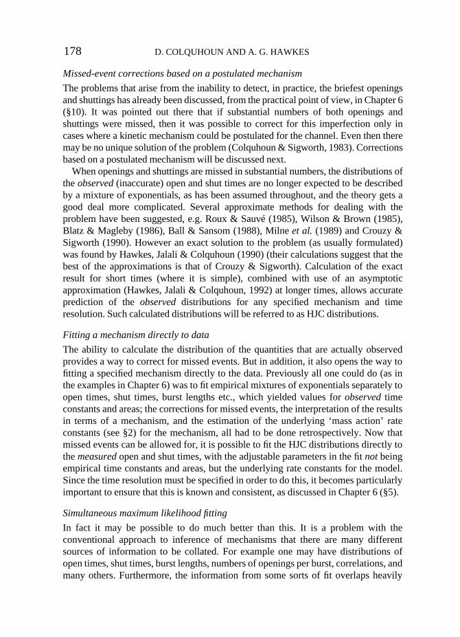
Missed-event corrections based on a postulated mechanism

The problems that arise from the inability to detect, in practice, the briefest openingsand shuttings has already been discussed, from the practical point of view, in Chapter 6(§10). It was pointed out there that if substantial numbers of both openings andshuttings were missed, then it was possible to correct for this imperfection only incases where a kinetic mechanism could be postulated for the channel. Even then theremay be no unique solution of the problem (Colquhoun & Sigworth, 1983). Correctionsbased on a postulated mechanism will be discussed next.

When openings and shuttings are missed in substantial numbers, the distributions ofthe observed(inaccurate) open and shut times are no longer expected to be describedby a mixture of exponentials, as has been assumed throughout, and the theory gets agood deal more complicated. Several approximate methods for dealing with theproblem have been suggested, e.g. Roux & Sauvé (1985), Wilson & Brown (1985),Blatz & Magleby (1986), Ball & Sansom (1988), Milne et al. (1989) and Crouzy &Sigworth (1990). However an exact solution to the problem (as usually formulated)was found by Hawkes, Jalali & Colquhoun (1990) (their calculations suggest that thebest of the approximations is that of Crouzy & Sigworth). Calculation of the exactresult for short times (where it is simple), combined with use of an asymptoticapproximation (Hawkes, Jalali & Colquhoun, 1992) at longer times, allows accurateprediction of the observeddistributions for any specified mechanism and timeresolution. Such calculated distributions will be referred to as HJC distributions.

Fitting a mechanism directly to data

The ability to calculate the distribution of the quantities that are actually observedprovides a way to correct for missed events. But in addition, it also opens the way tofitting a specified mechanism directly to the data. Previously all one could do (as inthe examples in Chapter 6) was to fit empirical mixtures of exponentials separately toopen times, shut times, burst lengths etc., which yielded values for observedtimeconstants and areas; the corrections for missed events, the interpretation of the resultsin terms of a mechanism, and the estimation of the underlying ‘mass action’ rateconstants (see §2) for the mechanism, all had to be done retrospectively. Now thatmissed events can be allowed for, it is possible to fit the HJC distributions directly tothe measuredopen and shut times, with the adjustable parameters in the fit notbeingempirical time constants and areas, but the underlying rate constants for the model.Since the time resolution must be specified in order to do this, it becomes particularlyimportant to ensure that this is known and consistent, as discussed in Chapter 6 (§5).

Simultaneous maximum likelihood fitting

In fact it may be possible to do much better than this. It is a problem with theconventional approach to inference of mechanisms that there are many differentsources of information to be collated. For example one may have distributions ofopen times, shut times, burst lengths, numbers of openings per burst, correlations, andmany others. Furthermore, the information from some sorts of fit overlaps heavily


(e.g. the distribution of total open time per burst may be very similar to thedistribution of burst length) so it can be a problem to decide how many such things tocalculate.

However, once one can calculate the probability (density) for the observedopenand shut time, by means of the HJC distributions, or approximations to them, then itbecomes feasible to calculate the likelihood (see Chapter 6) of an entire singlechannel record (see Horn & Lange, 1983; Horn & Vandenberg, 1984; Fredkin &Rice, 1992). This means that, in order to do the fitting, we do not have to fit separatelyall of the sorts of distribution mentioned above; instead we simply adjust theparameters (mass action rate constants) so as to maximise the likelihood for the entirerecord. This takes into account simultaneouslythe information from the open times,from the shut times and from the order in which they occur(i.e. from the burststructure and from correlations between events). We have found this to be quitefeasible on a fast PC, at least for a few thousands of observations. Further than this, italso becomes feasible to fit several different sorts of measurement simultaneously,for example recordings made with different concentrations of agonist (Hawkes et al.,in preparation).

This approach can be used to judge the relative merits of alternative postulatedmechanisms. If each of the proposed mechanisms is fitted to the same data, therelative plausibility of each mechanism can be assessed from how large its likelihoodis. This has been done, for example, by Horn & Vandenberg (1984) (without missedevent correction).

An example of fitting with missed events

An example of maximum likelihood fitting by the HJC method (to simulated singlechannel data) is shown in Fig. 12.

The data in the histograms in Fig. 12 were simulated using the 5-state model for thenicotinic acetylcholine receptor, with the rate constants and concentration used byColquhoun & Hawkes (1982) as shown in (8.1). The numbers are transition rates ins−1 (see discussion following 2.1).

A resolution of 100 µs (for both open and shut times) was then imposed on the

(8.1)


simulated sequence of open and shut times (see Chapter 6), to produce a sequence ofapparentopen and shut times from which the histograms were constructed. Thesehistograms were not themselves fitted, but the likelihood of the entire sequence ofapparent open and shut times was calculated, as outlined above, and the free


196

144

100

64

36

16

4

0

256

Fre

quen

cy (

squa

re r

oot s

cale

)

1 10

A

1000.01 0.1

Apparent open time (ms) (log scale)

true pdf (scaled)

484

400

0

4

16

36

64

100

144

196

256

324

Fre

quen

cy (

squa

re r

oot s

cale

)

B

0.1 1 10 100 1000 10000 1000000.01

Apparent shut time (ms) (log scale)

true pdf (scaled)

Fig. 12. Example of the effect of missed events. The 5-state mechanism in (8.1) was used tosimulate 10235 channel transitions. A resolution of 100 µs was imposed on the simulatedchannels resulting in 3419 resolved intervals, from which the histograms of apparent opentines (A), and apparent shut times (B) were constructed. The continuous lines are the HJCdistributions calculated for a resolution of 100 µs with rate constants as in (8.1); the exactsolution is used for intervals up to 300 µs, and the asymptotic solution thereafter. The dashedlines show the true open and shut time distributions.

parameters adjusted (by the simplex method) to maximize this likelihood. Theestimates of the transition rates, from this singlefitting procedure, were close to thevalues shown in (8.1), as hoped. The true values from (8.1) were then used tocalculate the HJC distributions for the apparentopen times and shut times. These areshown as continuous lines superimposed on the histograms in Fig. 12. It can be seenthat they fit the ‘observations’ quite well. The same values were then used to calculatethe predicted open and shut time distributions by the standard methods (e.g.Colquhoun & Hawkes, 1982), with no allowance for missed events. Thesedistributions, which are what would be expected if we had perfect time resolution, areshown as dashed lines in Fig. 12A,B.

The open time distribution in Fig. 12A shows that the openings appear to beconsiderably longer than their true values, because many brief shuttingsare below the100 µs resolution, and therefore not detected. The true fast shut time component hasτ=52.6 µs, so 85% of this component is missed. With perfect resolution the open timedistribution would, with the rate constants in (8.1), have two exponential componentswith τ=2.0 ms (93% of area) and τ=0.33 ms (7% of area). The asymptotic HJCdistribution of apparent open times, on the other hand, has components with τ=6.1 ms(81% of area) and 0.33 ms (19% of area).

The shut time distribution in Fig. 12B shows, in contrast, that the distribution ofapparent shut times is close to the true distribution, except of course that there are noshut times below 100 µs: this happens because, in this particular example, relativelyfew openingsare below 100 µs. This shows, incidentally, that for results of this sort,the number of missed shuttings can be estimated quite accurately by extrapolating theshut time distribution to zero length. Thus the crude form of retrospective missedevent correction used by Colquhoun & Sakmann (1985) (see also Chapter 6) shouldhave been reasonably accurate.

Problems: the number of channels

Perhaps the biggest single problem that hinders the interpretation of single channelrecords stems from the fact that one rarely knows how many functional channels werepresent in the membrane patch from which the record was made. Shut timedistributions, including first latency distributions, must obviously depend on thenumber of channels that are present.

If it is observed, at any time during the recording, that more than one channel isopen, then the patch must contain more than one channel, but it is notoriouslydifficult to estimate how many there are, at least when Popenis low (see Horn, 1991,and Chapter 6, §5). A method based on the length of runs of single openings has beenproposed (Colquhoun & Hawkes, 1990), which may be useful if the burst structure ofthe data is not too complex.

Perhaps the most common way of managing this problem is to confine attentiononly to subsections of the record that can, with confidence, be attributed to the activityof only one channel. Such subsections may consist of individual bursts (e.g. at lowagonist concentrations), or may consist of much longer clusters of openings when


Popenis high (see Chapter 6). This means, of course, that information from longer shutperiods is lost. This approach can be incorporated into maximum likelihood fittingwith HJC distributions (Hawkes, Jalali, & Colquhoun, in preparation).

Problems: indeterminacy of parameters

It is unlikely that any individual experimental record will contain enoughinformation to allow estimation of all the rate constants in the postulatedmechanism. This problem can be minimized if several sorts of experiment (e.g.equilibrium records with different ligand concentrations, jump experiments, Popen

curves etc.) can be analysed simultaneously, as described above. But in practice itwill often be necessary to estimate some rate constants form one sort of experiment,and then to treat these values as fixed while estimating others from a different sort ofexperiment (see, for example, Colquhoun & Sakmann, 1985; Sine, Claudio &Sigworth, 1990).

Problems: indeterminacy of mechanisms

It is well-known that kinetic mechanisms are not unique. Whatever mechanism isproposed, it will virtually always be possible to find another mechanism that fits theexperimental results just as well. Some classes of mechanism predict results that aretoo similar for them to be distinguished in practice. Worse still, some classes ofmechanism are indistinguishable in principle; this has been discussed very elegantlyby Kienker (1989). Nevertheless, combination of different sorts of biophysicalexperiment (as in the last paragraph), together with biochemical and structuralinformation, can do much to reduce the ambiguity.

These problems lead some people to be pessimistic about the possibility ofinterpreting experiments in terms of physical mechanisms. One extreme reaction is topoint out that proteins have an essentially infinite number of conformations (which is,no doubt, true), and must therefore be analysed by fractal methods, with consequentdenial that anything can be gleaned about the physical mechanisms involved (see. forexample, Korn & Horn, 1988). We think that it is perverse to suggest thatexperimental results have not been able to cast light on topics such as mechanisms ofion channel block, or the fine structure of bursts; the proposed mechanisms aredoubtless approximations, but they are not baseless.

Appendix 1. Derivation of the shut time distribution for theCastillo-Katz mechanism

The Castillo-Katz mechanism defined in (4.1) will be written again here, for easyreference.


The derivation is fairly lengthy, even for this mechanism with only three states.This complexity results, to a great extent, from the fact that the two shut states caninterconvert directly (unlike the simple channel block mechanism), so that there maybe any number of oscillations between them during any individual shut period. It caneasily be imagined that derivations such as that to follow are not generally feasible formechanisms with more than three states, and even with three states the complexity isgreat enough to provide a considerable incentive to program the quite general matrixresults (Colquhoun & Hawkes, 1982) which will give numerical results for anymechanism.

First, notice that when the channel is at equilibrium, everyshut period follows anopening, and so must start with a sojourn in the intermediate complex, AR (state 2).After leaving AR the channel may reopen immediately, or it may go through anynumber of AR[R oscillations before reopening. Furthermore every shut period mustend in state 2 (AR) also, because the shut period ends when an opening occurs, andopening is possible only from state 2.

We start by defining the probability, denoted P22(t), that the channel starts in state2, stays shut (state 2 or 3) throughoutthe time period from 0 to t, and is in state 2 at t.The shut lifetime will be t if, having stayed shut throughout the time from 0 to t, thechannel then opens. The probability that a channel opens during a small timeinterval, ∆t, is, by analogy with (2.10), β∆t. The probability density function for allshut times, fs(t) say, can be found by multiplying these two probabilities (theprobabilities are independent, because the probability of a transition from state 2 tostate 1 in the interval between t and t+∆t is independent of the previous history of theprocess): it is, therefore, the limiting value, for very small ∆t, of the followingexpression.

fs(t) = Prob[channel shut from 0 to t and opens during t, t+∆t]/∆t

= P22(t)β (A1.2)

We can now get an expression for P22(t), in the following way. The channel will bein state 2 (AR) at time t+∆t if either (1) it was in state 2 at time t, and fails to leavestate 2 during ∆t, or (2) it was in state 3 (R) at time t, andmoves from 2 to 3 (i.e. bindsa ligand molecule) during ∆t. To evaluate the first of these contingencies, we note thatthe probability of leaving state 2 (for either state 3 or state 1) during ∆t is (β+k−1)∆t,so the probability of not leaving is 1 minus this quantity. To evaluate the second term

vacant

shut open

state number: 3 2 1

occupied

A + R [ AR[ AR*k+1 β

αk−1 (A1.1)


we must first define P23(t) as the probability that a channel that is in state 2 at t=0 thenremains shut throughout the time from 0 to t and is in state 3 at t; the probability of atransition from 3 to 2 in ∆t is then k+1xA∆t. We can now assemble all the possibilitiesto write

P22(t + ∆t) = P22(t)[1 − (β + k−1)∆t] + P23(t)k+1xA∆t . (A1.3)

Thus

and so, letting ∆t→0, we obtain

This equation contains two unknowns, P22(t) and P23(t). To solve this problem wemust go through an exactly analogous argument to obtain a second equation, viz.

These two equations allow the two unknowns to be evaluated. To achieve this weeliminate P23(t) from the equations by using (A1.5) to obtain an expression for P23(t),which is then substituted into (A1.6). The result is a second order equation thatinvolves only P22(t), thus

If we define the (constant) coefficients, b and c, as

b = λ1 + λ2 = β + k−1 + k+1xA (A1.8)

c = λ1λ2 = k+1xAβ (A1.9)

then (A1.7) can be written in the form

We are now in a position to obtain expressions for the observed time constants. Asolution of (A1.10) is needed, and we proceed, in the irritating manner ofmathematicians, to propose, for no apparent reason, that there is a particular solutionof (A1.10) that has the form P22(t)=e−λt. If this is the case then dP22(t)/dt=−λe−λt, andd2P22(t)/dt2=λ2e−λt. Substitution of these into (A1.10) gives:

––––––– + b ––––––– + cP22(t) = 0d2P22(t)

dt2dP22(t)

dt(A1.10)

–––––––– + (β + k−1 + k+1xA) ––––––– + k+1xAβP22(t) = 0d2P22(t)

dt2dP22(t)

dt(A1.7)

–––––––– = P22(t) k−1 − P23(t)k+1xA .dP23(t)

dt(A1.6)

–––––––– = − P22(t)(β + k−1) + P23(t)k+1xAdP22(t)

dt(A1.5)

–––––––––––––––– = − P22(t)(β + k−1) + P23(t)k+1xAP22(t+∆t) − P22(t)

∆t(A1.4)


λ2e−λt − bλe−λt + ce−λt = 0 (A1.11)

This result must be true at all times, including at t=0. Putting t=0 in (A1.11) gives

λ2 − bλ + c = 0 (A1.12)

This is a quadratic equation and therefore there will generally be two values of theobservedrate constants, λ1 and λ2 say, that satisfy it, and these can be found as thetwo solutions of (A1.12), namely

or

where the coefficients, b and c, were defined in (A1.8) and (A1.9). Notice that thesecoefficients are rather simpler than those given in (5.4) and (5.5) for the macroscopicrelaxation, because we are now dealing only with the shut states. They no longerinvolve all of the fundamental rate constants (α does not appear).

To complete the distribution of shut times, we must next find the areas, a1 and a2,of the two components. The p.d.f. has the form (see Chapter 6)

fs(t) = βP22(t) = a1λ1e−λ1t + a2λ2e−λ2t (A1.15)

where a2=1−a1, because the total are must be 1. Thus, from (A1.2) and (A1.15),

The last line follows from (A1.5) because P22(0)=1 (state 2 cannot be left in zerotime), and P23(0)=0 (cannot get from state 2 to 3 in zero time). From this, togetherwith the fact that λ1+λ2=β+k−1+k+1xA and λ1λ2=k+1xAβ (see A1.8 and A1.9), we find,after some manipulation, that the areas of the two components are given by

This completes the derivation of the distribution of all shut times. The same resultwas derived, in a quite different way, by Colquhoun & Hawkes (1981), but if all thatis needed is numerical values for the time constants and areas of the components it isobviously much easier to use the entirely general result (Colquhoun & Hawkes,

a1 = –––––––––––– , and a2 = 1 − a1 .β(k+1xA − λ1)

(λ2 − λ1)λ1

(A1.17)

–––––– = –––––– = − a1λ12 − a2λ2

2dfs(t) βdP22(t)dt dtt=0 t=0

(A1.16)

= a1(λ22 − λ1

2 ) − λ22

= −β(β + k−1)

λ1, λ2 = –––––––––––– ,b7√b2 − 4c

2c (A1.14)

λ1, λ2 = 0.5sb ± √b2 − 4cd (A1.13)


1982), rather than go through a derivation like that above for every mechanism ofinterest.

Approximations for the time constants.If b2 » 4c then it follows from (A1.13) thatone of the observed rate constants will be much larger than the other, say λ2 » λ1. Thiswill be the case, for example, when the ligand concentration, xA, is very low, so from(A1.8), we find that the faster time constant is approximately

The right hand side of this is simply the mean lifetime of a single sojourn in theintermediate complex AR (state 2). This is, therefore, an example of a case where,contrary to the general rule, a physical interpretation can be placed on an observedtime constant, as an approximation. In this case the sojourns in AR that occur as thechannel oscillates between AR[AR*, can be seen (approximately) as the fastcomponent of the distribution of all shut times.

References

ADAMS, P. R. (1976). Drug blockade of open end-plate channels.J. Physiol.260, 531-552. ADAMS, P. R. & SAKMANN, B. (1978). Decamethonium both opens and blocks endplate channels.

Proc. Natl. Acad. Sci. U.S.A. 75, 2994-2998.ALDRICH, R. W., COREY, D. P. & STEVENS, C. F. (1983). A reinterpretation of mammalian sodium

channel gating based on single channel recording. Nature306, 436-441.ANDERSON, C. R. & STEVENS, C. F. (1973). Voltage clamp analysis of acetylcholine produced end-

plate current fluctuations at frog neuromuscular junction. J. Physiol.235, 655-691.BALL, F. G. & SANSOM, M. S. P. (1988). Aggregated Markov processes incorporating time interval

omission. Adv. Appl. Prob.20, 546-572.BALL, F. G. & SANSOM, M. S. P. (1988). Single channel autocorrelation functions. The effects of time

interval omission. Biophys. J.53, 819-832.BLATZ, A. L. & MAGLEBY, K. L. (1986). Correcting single channel data for missed events. Biophys.

J. 49, 967-980.BLATZ, A. L. & MAGLEBY, K. L. (1989). Adjacent interval analysis distinguishes among gating

mechanisms for the fast chloride channel from rat skeletal muscle. J. Physiol.410, 561-585.CASTILLO, J. del & KATZ, B. (1957). Interaction at end-plate receptors between different choline

derivatives. Proc. Roy. Soc.B 146, 369-381. COLQUHOUN, D. (1971). Lectures on Biostatistics.Oxford: Clarendon Press. COLQUHOUN, D., DREYER, F. & SHERIDAN, R. E. (1979). The actions of tubocurarine at the frog

neuromuscular junction. J. Physiol.293, 247-284. COLQUHOUN, D. & HAWKES, A. G. (1977). Relaxation and fluctuations of membrane currents that

flow through drug-operated ion channels. Proc. Roy. Soc.B 199, 231-262.COLQUHOUN, D. & HAWKES, A. G. (1981). On the stochastic properties of single ion channels.

Proc. Roy. Soc.B 211, 205-235. COLQUHOUN, D. & HAWKES, A. G. (1982). On the stochastic properties of bursts of single ion

channel openings and of clusters of bursts. Phil. Trans. Roy. Soc.B 300, 1-59.COLQUHOUN, D. & HAWKES, A. G. (1983). The principles of the stochastic interpretation of ion

channel mechanisms. In Single Channel Recording(ed. B. Sakmann & E. Neher). New York: PlenumPress.

COLQUHOUN, D. & HAWKES A. G. (1987). A note on correlations in single channel records. Proc.Roy. Soc. B 230, 15-52.

COLQUHOUN, D. & HAWKES, A. G. (1990). Stochastic properties of ion channel openings and bursts

τ2 = 1/λ2 ≈ –––––––1

β + k−1(A1.18)


in a membrane patch that contains two channels: evidence concerning the number of channels presentwhen a record containing only single openings is observed. Proc. Roy. Soc. LondonB 240, 453-477.

COLQUHOUN, D., JONAS, P. & SAKMANN, B. (1992). Action of brief pulses of glutamate onAMPA/kainate receptors in patches from different neurones of rat hippocampal slices.J. Physiol.458,261-287.

COLQUHOUN, D. & OGDEN, D. C. (1986). States of the acetylcholine receptor: enumerationcharacteristics and structure. In Nicotinic Acetylcholine Receptor: structure and function(ed. A.Maelicke). Berlin: Springer-Verlag. pp. 197-232.

COLQUHOUN, D., OGDEN. D. C. & CACHELIN, A. B. (1986). Mode of action of agonists onnicotinic receptors. In Ion Channels in Neural Membranes(ed. J. M. Ritchie, R. D. Keynes &L.Bolis), pp. 255-273. New York: A. R. Liss.

COLQUHOUN, D. & SAKMANN, B. (1981). Fluctuations in the microsecond time range of the currentthrough single acetylcholine receptor ion channels. Nature294, 464-466.

COLQUHOUN, D. & SAKMANN, B. (1983). Bursts of openings in transmitter-activated ion channels.In Single Channel Recording (ed. B. Sakmann & E. Neher). New York: Plenum Press.

COLQUHOUN, D. & SAKMANN, B. (1985). Fast events in single-channel currents activated byacetylcholine and its analogues at the frog muscle end-plate. J. Physiol.369, 501-557.

COLQUHOUN, D . & SHERIDAN R. E. (1981) . The modes of action of gallamine. Proc. Roy. Soc.LondonB 211, 181-203.

CROUZY, S. C. & SIGWORTH, F. J. (1990). Yet another approach to the dwell-time omission problemof single-channel analysis. Biophys. J.58, 731-743.

EDMONDS, B. & COLQUHOUN, D. (1992). Rapid decay of averaged single-channel NMDA receptoractivations recorded at low agonis concentration. Proc. Roy. Soc. LondonB, 250, 279-286.

FRANKE, CH., HATT, H., PARNAS, H. & DUDEL, J. (1991). Kinetic constants of the acetylcholine(ACh) receptor reaction deduced from the rise in open probability after steps in ACh concentration.Biophys. J.60, 1008-1016.

FREDKIN, D. R., MONTAL, M. & RICE, J. A. (1985). Identification of aggregated Markovian models:application to the nicotinic acetylcholine receptor. In: Proceedings of the Berkeley Conference inhonor of Jerzy Neyman and Jack Kiefer, vol. I (ed. L. M. Le Carn & R. A. Olshen). pp. 269-289.Wadsworth Press.

FREDKIN, D. R. & RICE, J. A. (1992). Maximum likelihood estimation and identification directly fromsingle-channel recordings. Proc. Roy. Soc. London B 249, 125-132.

GIBB, A. J. & COLQUHOUN, D. (1992). Activation of NMDA receptors by L-glutamate in cellsdissociated from adult rat hippocampus. J. Physiol. 456, 143-179.

HAMILL, O. P., MARTY, A., NEHER, E., SAKMANN, B. & SIGWORTH, F. J. (1981). Improvedpatch-clamp techniques for high-resolution current recording from cells and cell-free membranepatches. Pflugers Archiv.391, 85-100.

HAWKES, A. G., JALALI, A. & COLQUHOUN, D. (1990). The distributions of the apparent opentimes and shut times in a single channel record when brief events can not be detected. Phil. Trans.Roy. Soc. LondonA 332, 511-538.

HAWKES, A.G., JALALI, A. & COLQUHOUN, D. (1992). Asymptotic distributions of apparent opentimes and shut times in a single channel record allowing for the omission of brief events. Phil. Trans.Roy. Soc. London B 337, 383-404.

HORN, R. (1991). Estimating the number of channels in patch recordings. Biophys. J.60, 433-439.HORN, R. (1984). Gating of channels in nerve and musclc: a stochastic approach. In Ion Channels:

Molecular and Physiological Aspects(ed. W. D. Stein). pp. 53-97. New York: Academic Press. HORN, R. & LANGE, K. (1983). Estimating kinetic constants from single channel data. Biophys. J.43,

207-223.HORN, R. & VANDENBURG, C. A. (1984). Statistical properties of single sodium channels. J. Gen.

Physiol.84, 505-534.JACKSON, M. B., WONG, B. S., MORRIS, C. E., LECAR, H. & CHRISTIAN, C. N. (1983).

Successive openings of the same acetylcholine receptor channels are correlated in open time. Biophys.J. 42, 109-114.

KIENKER, P. (1989). Equivalence of aggregated Markov models of ion-channel gating. Proc. Roy. Soc.LondonB 236, 269-309.

KORN, J. S. & HORN, R. (1988). Statistical discrimination of fractal and Markov models of single-channel gating. Biophys. J.54, 871-877.


LABARCA, P., RICE, J. A., FREDKIN, D. R. & MONTAL, M. (1985). Kinetic analysis of channelgating: application to the cholinergic receptor channel and the chloride channel from Torpedocalifornica. Biophys. J.47, 469-478.

LIU, Y. & DILGER, J. P. (1991). Opening rate of acetylcholine receptor channels. Biophys. J.60, 424-432.

MAGLEBY, K. L. & WEISS, D. S. (1990). Identifying kinetic gating mechanisms for ion channels byusing two-dimensional distributions of simulated dwell times. Proc. Roy. Soc. LondonB 241, 220-228.

McMANUS, O. B., BLATZ, A. L. & MAGLEBY, K. L. (1985). Inverse relationship of the durations ofopen and shut intervals for Cl and K channels. Nature317, 625-627.

MILNE, R. K., YEO, G. F., EDESON, R. O. & MADSEN, B. W. ( 1989). Estimation of single channelkinetic parameters from data subject to limited time resolution. Biophys. J. 55, 673-676.

NEHER, E. (1983). The charge carried by single-channel currents of rat cultured muscle cells in thepresence of local anaesthetics. J. Physiol.339, 663-678.

NEHER, E. & STEINBACH, J. H. (1978). Local anaesthetics transiently block currents through singleacetylcholine-receptor channels. J. Physiol.277, 153-176.

OGDEN, D. C. & COLQUHOUN, D. (1985). Ion channel block by acetylcholine, carbachol andsuberyldicholine at the frog neuromuscular junction. Proc. Roy. Soc. LondonB 225, 329- 355.

OGDEN, D. C., SIEGELBAUM, S. A. & COLQUHOUN, D. (1981). Block of acetylcholine- activatedion channels by an uncharged local anaesthetic. Nature289, 596-599.

ROUX, B. & SAUVE, R. (1985). A general solution to the time interval omission problem applied tosingle channel analysis. Biophys. J.48, 149-158.

SAKMANN, B., PATLAK, J. & NEHER, E. (1980). Single acetylcholine-activated channels showburst-kinetics in presence of desensitizing concentrations of agonist. Nature286, 72-73.

SAKMANN, B. & TRUBE, G. (1984). Voltage-dependent inactivation of inward-rectifying singlechannel currents in the guinea-pig heart cell membrane. J. Physiol.347, 659-683.

SINE, S. M. & STEINBACH, J. H. (1986). Activation of acetylcholine receptors on clonal BC3H-1 cellsby low concentrations of agonist. J. Physiol.373, 129-162.

SINE, S. M., CLAUDIO, T. & SIGWORTH, F. J. (1990). Activation of Torpedo acetylcholine receptorsexpressed in mouse fibroblasts: single channel current kinetics reveal distinct agonist bindingaffinities. J. Gen. Physiol.96, 395-437.

THOMPSON, S.P. (1965). Calculus Made Easy. London: Macmillan. WILSON, D. L. & BROWN, A. M. (1985). Effect of limited interval resolution on single channel

measurements with application to Ca channels. IEEE Trans. Biomed. Eng.32, 780-797.


the interpretation of single channel recordingstres/microelectrode/microelectrodes_ch07.pdf · 141...

Documents