the joint s&p 500/vix smile calibration puzzle solved
TRANSCRIPT

Motivation Dispersion-constrained martingale optimal transport VIX-constrained martingale Schrodinger bridges Inversion of cvx ordering
The Joint S&P 500/VIX Smile Calibration Puzzle Solved
Julien Guyon
Bloomberg, Quantitative Research
Mathematical Finance & Financial Data Science Seminar
NYU CourantJanuary 26, 2021
Julien Guyon c© 2021 Bloomberg Finance L.P. All rights reserved.
The Joint S&P 500/VIX Smile Calibration Puzzle Solved

Motivation Dispersion-constrained martingale optimal transport VIX-constrained martingale Schrodinger bridges Inversion of cvx ordering
Motivation
Volatility indices, such as the VIX index, are not only used asmarket-implied indicators of volatility.
Futures and options on these indices are also widely used asrisk-management tools to hedge the volatility exposure of optionsportfolios.
The very high liquidity of S&P 500 (SPX) and VIX derivatives requiresthat financial institutions price, hedge, and risk-manage their SPX andVIX options portfolios using models that perfectly fit market prices ofboth SPX and VIX futures and options, jointly.
Calibration of stochastic volatility models to liquid hedging instruments:SPX options + VIX futures and options.
Since VIX options started trading in 2006, many researchers andpractitioners have tried to build such a jointly calibrating model, but couldonly, at best, get approximate fits.
“Holy Grail of volatility modeling”
Very challenging problem, especially for short maturities.
Julien Guyon c© 2021 Bloomberg Finance L.P. All rights reserved.
The Joint S&P 500/VIX Smile Calibration Puzzle Solved

Motivation Dispersion-constrained martingale optimal transport VIX-constrained martingale Schrodinger bridges Inversion of cvx ordering
Motivation
Figure: SPX smile as of January 22, 2020, T = 30 days
Julien Guyon c© 2021 Bloomberg Finance L.P. All rights reserved.
The Joint S&P 500/VIX Smile Calibration Puzzle Solved
Motivation Dispersion-constrained martingale optimal transport VIX-constrained martingale Schrodinger bridges Inversion of cvx ordering
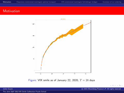
Motivation
Figure: VIX smile as of January 22, 2020, T = 28 days
Julien Guyon c© 2021 Bloomberg Finance L.P. All rights reserved.
The Joint S&P 500/VIX Smile Calibration Puzzle Solved
Motivation Dispersion-constrained martingale optimal transport VIX-constrained martingale Schrodinger bridges Inversion of cvx ordering
Motivation
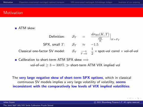
ATM skew:
Definition: ST =dσBS(K,T )
dKK
∣∣∣K=FT
SPX, small T : ST ≈ −1.5
Classical one-factor SV model: ST −→T→0
1
2× spot-vol correl× vol-of-vol
Calibration to short-term ATM SPX skew =⇒vol-of-vol ≥ 3 = 300%� short-term ATM VIX implied vol
The very large negative skew of short-term SPX options, which in classicalcontinuous SV models implies a very large volatility of volatility, seems
inconsistent with the comparatively low levels of VIX implied volatilities.
Julien Guyon c© 2021 Bloomberg Finance L.P. All rights reserved.
The Joint S&P 500/VIX Smile Calibration Puzzle Solved

Motivation Dispersion-constrained martingale optimal transport VIX-constrained martingale Schrodinger bridges Inversion of cvx ordering
Gatheral (2008)
Julien Guyon c© 2021 Bloomberg Finance L.P. All rights reserved.
The Joint S&P 500/VIX Smile Calibration Puzzle Solved

Motivation Dispersion-constrained martingale optimal transport VIX-constrained martingale Schrodinger bridges Inversion of cvx ordering
Julien Guyon c© 2021 Bloomberg Finance L.P. All rights reserved.
The Joint S&P 500/VIX Smile Calibration Puzzle Solved

Motivation Dispersion-constrained martingale optimal transport VIX-constrained martingale Schrodinger bridges Inversion of cvx ordering
Julien Guyon c© 2021 Bloomberg Finance L.P. All rights reserved.
The Joint S&P 500/VIX Smile Calibration Puzzle Solved

Motivation Dispersion-constrained martingale optimal transport VIX-constrained martingale Schrodinger bridges Inversion of cvx ordering
Julien Guyon c© 2021 Bloomberg Finance L.P. All rights reserved.
The Joint S&P 500/VIX Smile Calibration Puzzle Solved
Motivation Dispersion-constrained martingale optimal transport VIX-constrained martingale Schrodinger bridges Inversion of cvx ordering
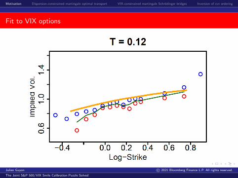
Fit to VIX options
Julien Guyon c© 2021 Bloomberg Finance L.P. All rights reserved.
The Joint S&P 500/VIX Smile Calibration Puzzle Solved

Motivation Dispersion-constrained martingale optimal transport VIX-constrained martingale Schrodinger bridges Inversion of cvx ordering
Fit to VIX options
Julien Guyon c© 2021 Bloomberg Finance L.P. All rights reserved.
The Joint S&P 500/VIX Smile Calibration Puzzle Solved

Motivation Dispersion-constrained martingale optimal transport VIX-constrained martingale Schrodinger bridges Inversion of cvx ordering
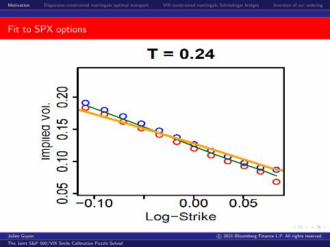
Fit to SPX options
Julien Guyon c© 2021 Bloomberg Finance L.P. All rights reserved.
The Joint S&P 500/VIX Smile Calibration Puzzle Solved
Motivation Dispersion-constrained martingale optimal transport VIX-constrained martingale Schrodinger bridges Inversion of cvx ordering
Fit to SPX options
Julien Guyon c© 2021 Bloomberg Finance L.P. All rights reserved.
The Joint S&P 500/VIX Smile Calibration Puzzle Solved

Motivation Dispersion-constrained martingale optimal transport VIX-constrained martingale Schrodinger bridges Inversion of cvx ordering
Similar experiments with other models
Skewed 2-factor Bergomi model (Bergomi 2008)
Skewed rough Bergomi model (G. 2018, De Marco 2018):
σ2t = ξt0
((1− λ)E
(ν0
∫ t
0
(t− s)H−12 dZs
)+ λE
(ν1
∫ t
0
(t− s)H−1/2dZs
))with λ ∈ [0, 1].
Quadratic rough Heston model (Gatheral Jusselin Rosenbaum 2020)
VIX smile well calibrated =⇒ not enough SPX ATM skew
Julien Guyon c© 2021 Bloomberg Finance L.P. All rights reserved.
The Joint S&P 500/VIX Smile Calibration Puzzle Solved

Motivation Dispersion-constrained martingale optimal transport VIX-constrained martingale Schrodinger bridges Inversion of cvx ordering
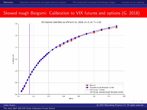
Skewed rough Bergomi: Calibration to VIX futures and options (G. 2018)
Julien Guyon c© 2021 Bloomberg Finance L.P. All rights reserved.
The Joint S&P 500/VIX Smile Calibration Puzzle Solved

Motivation Dispersion-constrained martingale optimal transport VIX-constrained martingale Schrodinger bridges Inversion of cvx ordering
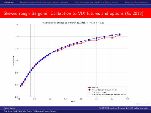
Skewed rough Bergomi: Calibration to VIX futures and options (G. 2018)
Julien Guyon c© 2021 Bloomberg Finance L.P. All rights reserved.
The Joint S&P 500/VIX Smile Calibration Puzzle Solved
Motivation Dispersion-constrained martingale optimal transport VIX-constrained martingale Schrodinger bridges Inversion of cvx ordering
Skewed rough Bergomi: Calibration to VIX futures and options (G. 2018)
Julien Guyon c© 2021 Bloomberg Finance L.P. All rights reserved.
The Joint S&P 500/VIX Smile Calibration Puzzle Solved

Motivation Dispersion-constrained martingale optimal transport VIX-constrained martingale Schrodinger bridges Inversion of cvx ordering
Skewed rough Bergomi: Calibration to VIX future and options (G. 2018)
Julien Guyon c© 2021 Bloomberg Finance L.P. All rights reserved.
The Joint S&P 500/VIX Smile Calibration Puzzle Solved

Motivation Dispersion-constrained martingale optimal transport VIX-constrained martingale Schrodinger bridges Inversion of cvx ordering
Skewed rough Bergomi calibrated to VIX: SPX smile (G. 2018)
Julien Guyon c© 2021 Bloomberg Finance L.P. All rights reserved.
The Joint S&P 500/VIX Smile Calibration Puzzle Solved

Motivation Dispersion-constrained martingale optimal transport VIX-constrained martingale Schrodinger bridges Inversion of cvx ordering
Quadratic rough Heston model (Gatheral Jusselin Rosenbaum 2020)
Julien Guyon c© 2021 Bloomberg Finance L.P. All rights reserved.
The Joint S&P 500/VIX Smile Calibration Puzzle Solved

Motivation Dispersion-constrained martingale optimal transport VIX-constrained martingale Schrodinger bridges Inversion of cvx ordering
Joint calibration of 2-factor Bergomi model to term-structure of SPX ATM
skew and VIX2 implied vol (G. 2020)
Figure: Left: ATM skew of SPX options as a function of maturity. Right: impliedvolatility of the squared VIX as a function of maturity. Calibration of theBergomi-Guyon expansion of the SPX ATM skew and a newly derived expansion of theVIX2 implied volatility, either jointly or separately. Calibration as of October 8, 2019
Julien Guyon c© 2021 Bloomberg Finance L.P. All rights reserved.
The Joint S&P 500/VIX Smile Calibration Puzzle Solved
Motivation Dispersion-constrained martingale optimal transport VIX-constrained martingale Schrodinger bridges Inversion of cvx ordering
Related works with continuous models on the SPX
Fouque-Saporito (2018), Heston with stochastic vol-of-vol. Problem: theirapproach does not apply to short maturities (below 4 months), for whichVIX derivatives are most liquid and the joint calibration is most difficult.
Goutte-Ismail-Pham (2017), Heston with parameters driven by a HiddenMarkov jump process.
Jacquier-Martini-Muguruza, On the VIX futures in the rough Bergomimodel (2017):
“Interestingly, we observe a 20% difference between the [vol-of-vol] pa-rameter obtained through VIX calibration and the one obtained throughSPX. This suggests that the volatility of volatility in the SPX marketis 20% higher when compared to VIX, revealing potential data incon-sistencies (arbitrage?).”
Guo-Loeper-Ob loj-Wang (2020): joint calibration via semimartingaleoptimal transport. Closely related to VIX-contrained martingaleSchrodinger bridges.
Julien Guyon c© 2021 Bloomberg Finance L.P. All rights reserved.
The Joint S&P 500/VIX Smile Calibration Puzzle Solved
Motivation Dispersion-constrained martingale optimal transport VIX-constrained martingale Schrodinger bridges Inversion of cvx ordering
Motivation
To try to jointly fit the SPX and VIX smiles, many authors haveincorporated jumps in the dynamics of the SPX: Sepp, Cont-Kokholm,Papanicolaou-Sircar, Baldeaux-Badran, Pacati et al, Kokholm-Stisen,Bardgett et al...
Jumps offer extra degrees of freedom to partly decouple the ATM SPXskew and the ATM VIX implied volatility.
So far all the attempts at solving the joint SPX/VIX smile calibrationproblem only produced an approximate fit.
Julien Guyon c© 2021 Bloomberg Finance L.P. All rights reserved.
The Joint S&P 500/VIX Smile Calibration Puzzle Solved

Motivation Dispersion-constrained martingale optimal transport VIX-constrained martingale Schrodinger bridges Inversion of cvx ordering
Exact joint calibrationvia dispersion-constrained
martingale optimal transport
(G. 2019)
Julien Guyon c© 2021 Bloomberg Finance L.P. All rights reserved.
The Joint S&P 500/VIX Smile Calibration Puzzle Solved

Motivation Dispersion-constrained martingale optimal transport VIX-constrained martingale Schrodinger bridges Inversion of cvx ordering
Exact joint calibration via dispersion-constrained MOT (G. 2019)
A completely different approach: instead of postulating a parametriccontinuous-time (jump-)diffusion model on the SPX, we build anonparametric discrete-time model:
Help to decouple SPX skew and VIX implied vol.Perfectly fits the smiles.
Given a VIX future maturity T1, we build a joint probability measure on(S1, V, S2) which is perfectly calibrated to the SPX smiles at T1 andT2 = T1 + 30 days, and the VIX future and VIX smile at T1.
S1: SPX at T1, V : VIX at T1, S2: SPX at T2.
Our model satisfies:Martingality constraint on the SPX;Consistency condition: the VIX at T1 is the implied volatility of the 30-daylog-contract on the SPX.
Our model is cast as the solution of a dispersion-constrained martingaletransport problem which is solved using the Sinkhorn algorithm, in thespirit of De March and Henry-Labordere (2019).
Julien Guyon c© 2021 Bloomberg Finance L.P. All rights reserved.
The Joint S&P 500/VIX Smile Calibration Puzzle Solved

Motivation Dispersion-constrained martingale optimal transport VIX-constrained martingale Schrodinger bridges Inversion of cvx ordering
Risk, April 2020
Julien Guyon c© 2021 Bloomberg Finance L.P. All rights reserved.
The Joint S&P 500/VIX Smile Calibration Puzzle Solved
Motivation Dispersion-constrained martingale optimal transport VIX-constrained martingale Schrodinger bridges Inversion of cvx ordering
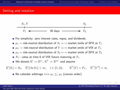
Setting and notation
S1, V
T1
S2
T230 days� -
For simplicity: zero interest rates, repos, and dividends.
µ1 = risk-neutral distribution of S1 ←→ market smile of SPX at T1.
µV = risk-neutral distribution of V ←→ market smile of VIX at T1.
µ2 = risk-neutral distribution of S2 ←→ market smile of SPX at T2.
FV : value at time 0 of VIX future maturing at T1.
We denote Ei := Eµi , EV := EµV and assume
Ei[Si] = S0, Ei[| lnSi|] <∞, i ∈ {1, 2}; EV [V ] = FV , EV [V 2] <∞.
No calendar arbitrage ⇐⇒ µ1 ≤c µ2 (convex order)
Julien Guyon c© 2021 Bloomberg Finance L.P. All rights reserved.
The Joint S&P 500/VIX Smile Calibration Puzzle Solved
Motivation Dispersion-constrained martingale optimal transport VIX-constrained martingale Schrodinger bridges Inversion of cvx ordering
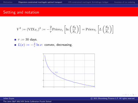
Setting and notation
V 2 := (VIXT1)2 := − 2
τPriceT1
[ln
(S2
S1
)]= PriceT1
[L
(S2
S1
)]τ := 30 days.
L(x) := − 2τ
lnx: convex, decreasing.
0 1 2 3 4 540
20
0
20
40
60
L(s)
Julien Guyon c© 2021 Bloomberg Finance L.P. All rights reserved.
The Joint S&P 500/VIX Smile Calibration Puzzle Solved

Motivation Dispersion-constrained martingale optimal transport VIX-constrained martingale Schrodinger bridges Inversion of cvx ordering
Superreplication, duality
Julien Guyon c© 2021 Bloomberg Finance L.P. All rights reserved.
The Joint S&P 500/VIX Smile Calibration Puzzle Solved

Motivation Dispersion-constrained martingale optimal transport VIX-constrained martingale Schrodinger bridges Inversion of cvx ordering
Superreplication of forward-starting options
The knowledge of µ1 and µ2 gives little information on the pricesEµ[g(S1, S2)], e.g., prices of forward-starting options Eµ[f(S2/S1)].
Computing upper and lower bounds of these prices:Optimal transport (Monge, 1781; Kantorovich)
Adding the no-arbitrage constraint that (S1, S2) is a martingale leads tomore precise bounds, as this provides information on the conditionalaverage of S2/S1 given S1:Martingale optimal transport (Henry-Labordere, 2017)
When S = SPX: Adding VIX market data information produces even moreprecise bounds, as it gives information on the conditional dispersion ofS2/S1, which is controlled by the VIX V :Dispersion-constrained martingale optimal transport
Julien Guyon c© 2021 Bloomberg Finance L.P. All rights reserved.
The Joint S&P 500/VIX Smile Calibration Puzzle Solved

Motivation Dispersion-constrained martingale optimal transport VIX-constrained martingale Schrodinger bridges Inversion of cvx ordering
Classical optimal transport
Figure: Example of a transport plan. Source: Wikipedia
Julien Guyon c© 2021 Bloomberg Finance L.P. All rights reserved.
The Joint S&P 500/VIX Smile Calibration Puzzle Solved

Motivation Dispersion-constrained martingale optimal transport VIX-constrained martingale Schrodinger bridges Inversion of cvx ordering
Superreplication: primal problem
Fundamental principle: Upper bound for the price of payoff f(S1, V, S2) =smallest price at time 0 of a superreplicating portfolio.
Following De Marco-Henry-Labordere (2015), G.-Menegaux-Nutz (2017), theavailable instruments for superreplication are:
At time 0:u1(S1): SPX vanilla payoff maturity T1 (including cash)u2(S2): SPX vanilla payoff maturity T2
uV (V ): VIX vanilla payoff maturity T1
Cost: MktPrice[u1(S1)] + MktPrice[u2(S2)] + MktPrice[uV (V )]= E1[u1(S1)] + E2[u2(S2)] + EV [uV (V )]
At time T1:∆S(S1, V )(S2 − S1): delta hedge∆L(S1, V )(L(S2/S1)− V 2): buy ∆L(S1, V ) log-contracts
Cost: 0
Shorthand notation:
∆(S)(s1, v, s2) := ∆(s1, v)(s2 − s1), ∆(L)(s1, v, s2) := ∆(s1, v)
(L
(s2
s1
)− v2
)Julien Guyon c© 2021 Bloomberg Finance L.P. All rights reserved.
The Joint S&P 500/VIX Smile Calibration Puzzle Solved

Motivation Dispersion-constrained martingale optimal transport VIX-constrained martingale Schrodinger bridges Inversion of cvx ordering
Superreplication: primal problem
The model-independent no-arbitrage upper bound for the derivative withpayoff f(S1, V, S2) is the smallest price at time 0 of a superreplicatingportfolio:
Pf := infUf
{E1[u1(S1)] + EV [uV (V )] + E2[u2(S2)]
}.
Uf : set of superreplicating portfolios, i.e., the set of all functions(u1, uV , u2,∆S ,∆L) that satisfy the superreplication constraint:
u1(s1) + uV (v) + u2(s2) + ∆(S)S (s1, v, s2) + ∆
(L)L (s1, v, s2) ≥ f(s1, v, s2).
Linear program.
Julien Guyon c© 2021 Bloomberg Finance L.P. All rights reserved.
The Joint S&P 500/VIX Smile Calibration Puzzle Solved

Motivation Dispersion-constrained martingale optimal transport VIX-constrained martingale Schrodinger bridges Inversion of cvx ordering
Superreplication: dual problem
P(µ1, µV , µ2): set of all the probability measures µ on R>0 × R≥0 × R>0
such that
S1 ∼ µ1, V ∼ µV , S2 ∼ µ2, Eµ [S2|S1, V ] = S1, Eµ[L
(S2
S1
)∣∣∣∣S1, V
]= V 2.
Dual problem:
Df := supµ∈P(µ1,µV ,µ2)
Eµ[f(S1, V, S2)].
Dispersion-constrained martingale optimal transport problem.
Eµ[S2|S1, V ] = S1: martingality condition of the SPX index, condition onthe average of the distribution of S2 given S1 and V .
Eµ[L(S2/S1)|S1, V ] = V 2: consistency condition, condition on dispersionaround the average.
Julien Guyon c© 2021 Bloomberg Finance L.P. All rights reserved.
The Joint S&P 500/VIX Smile Calibration Puzzle Solved

Motivation Dispersion-constrained martingale optimal transport VIX-constrained martingale Schrodinger bridges Inversion of cvx ordering
Superreplication: strong duality theorem (absence of a duality gap)
Theorem (G. 2020)
Let f : R>0 × R≥0 × R>0 → R be upper semicontinuous and satisfy
|f(s1, v, s2)| ≤ C(1 + s1 + s2 + |L(s1)|+ |L(s2)|+ v2)
for some constant C > 0. Then
Pf := infUf
{E1[u1(S1)] + EV [uV (V )] + E2[u2(S2)]
}= supµ∈P(µ1,µV ,µ2)
Eµ[f(S1, V, S2)] =: Df .
Moreover, Df 6= −∞ if and only if P(µ1, µV , µ2) 6= ∅, and in that case thesupremum is attained.
Julien Guyon c© 2021 Bloomberg Finance L.P. All rights reserved.
The Joint S&P 500/VIX Smile Calibration Puzzle Solved

Motivation Dispersion-constrained martingale optimal transport VIX-constrained martingale Schrodinger bridges Inversion of cvx ordering
Superreplication of forward-starting options
The knowledge of µ1 and µ2 gives little information on the pricesEµ[g(S1, S2)], e.g., prices of forward-starting options Eµ[f(S2/S1)].
Computing upper and lower bounds of these prices:Optimal transport (Monge, 1781; Kantorovich)
Adding the no-arbitrage constraint that (S1, S2) is a martingale leads tomore precise bounds, as this provides information on the conditionalaverage of S2/S1 given S1:Martingale optimal transport (Henry-Labordere, 2017)
When S = SPX: Adding VIX market data information produces even moreprecise bounds, as it information on the conditional dispersion of S2/S1,which is controlled by the VIX V :Dispersion-constrained martingale optimal transport
Adding VIX market data may possibly reveal a joint SPX/VIXarbitrage. Corresponds to P(µ1, µV , µ2) = ∅ (see next slides).
In the limiting case where P(µ1, µV , µ2) = {µ0} is a singleton, the jointSPX/VIX market data information completely specifies the jointdistribution of (S1, S2), hence the price of forward starting options.
Julien Guyon c© 2021 Bloomberg Finance L.P. All rights reserved.
The Joint S&P 500/VIX Smile Calibration Puzzle Solved
Motivation Dispersion-constrained martingale optimal transport VIX-constrained martingale Schrodinger bridges Inversion of cvx ordering
Joint SPX/VIX arbitrage
Julien Guyon c© 2021 Bloomberg Finance L.P. All rights reserved.
The Joint S&P 500/VIX Smile Calibration Puzzle Solved

Motivation Dispersion-constrained martingale optimal transport VIX-constrained martingale Schrodinger bridges Inversion of cvx ordering
Joint SPX/VIX arbitrage
U0 = the portfolios (u1, u2, uV ,∆S ,∆L) superreplicating 0:
u1(s1)+u2(s2)+uV (v)+∆S(s1, v)(s2−s1)+∆L(s1, v)
(L
(s2
s1
)− v2
)≥ 0
An (S1, S2, V )-arbitrage is an element of U0 with negative price:
MktPrice[u1(S1)] + MktPrice[u2(S2)] + MktPrice[uV (V )] < 0
Equivalently, there is an (S1, S2, V )-arbitrage if and only if
infU0
{MktPrice[u1(S1)] + MktPrice[u2(S2)] + MktPrice[uV (V )]} = −∞
Julien Guyon c© 2021 Bloomberg Finance L.P. All rights reserved.
The Joint S&P 500/VIX Smile Calibration Puzzle Solved

Motivation Dispersion-constrained martingale optimal transport VIX-constrained martingale Schrodinger bridges Inversion of cvx ordering
Consistent extrapolation of SPX and VIX smiles
If EV [V 2] 6= E2[L(S2)]−E1[L(S1)], there is a trivial (S1, S2, V )-arbitrage.For instance, if EV [V 2] < E2[L(S2)]− E1[L(S1)], pick
u1(s1) = L(s1), u2(s2) = −L(s2), uV (v) = v2, ∆S(s1, v) = 0, ∆L(s1, v) = 1.
=⇒ We assume that
EV [V 2] = E2[L(S2)]− E1[L(S1)]. (2.1)
Violations of (2.1) in the market have been reported, suggesting arbitrageopportunities, see, e.g., Section 7.7.4 in Bergomi (2016).
However, the quantities in (2.1) do not purely depend on market data.They depend on smile extrapolations.
The reported violations of (2.1) actually rely on some arbitrary smileextrapolations.
G. (2018) explains how to build consistent extrapolations of the VIXand SPX smiles so that (2.1) holds.
Julien Guyon c© 2021 Bloomberg Finance L.P. All rights reserved.
The Joint S&P 500/VIX Smile Calibration Puzzle Solved

Motivation Dispersion-constrained martingale optimal transport VIX-constrained martingale Schrodinger bridges Inversion of cvx ordering
Joint SPX/VIX arbitrage
Theorem (G. 2020)
The following assertions are equivalent:
(i) The market is free of (S1, S2, V )-arbitrage,
(ii) P(µ1, µV , µ2) 6= ∅,(iii) There exists a coupling ν of µ1 and µV such that Lawν(S1, L(S1) + V 2)
and Lawµ2(S2, L(S2)) are in convex order, i.e., for any convex functionf : R>0 × R→ R,
Eν [f(S1, L(S1) + V 2)] ≤ E2[f(S2, L(S2))].
Julien Guyon c© 2021 Bloomberg Finance L.P. All rights reserved.
The Joint S&P 500/VIX Smile Calibration Puzzle Solved

Motivation Dispersion-constrained martingale optimal transport VIX-constrained martingale Schrodinger bridges Inversion of cvx ordering
Build a model in P(µ1, µV , µ2)
Julien Guyon c© 2021 Bloomberg Finance L.P. All rights reserved.
The Joint S&P 500/VIX Smile Calibration Puzzle Solved

Motivation Dispersion-constrained martingale optimal transport VIX-constrained martingale Schrodinger bridges Inversion of cvx ordering
Build a model in P(µ1, µV , µ2)
Recall P(µ1, µV , µ2) := probability measures on R>0 × R≥0 × R>0 s.t.
S1 ∼ µ1, V ∼ µV , S2 ∼ µ2, Eµ [S2|S1, V ] = S1, Eµ[L
(S2
S1
)∣∣∣∣S1, V
]= V 2.
Build a model µ ∈ P(µ1, µV , µ2) = solve the joint calibration puzzle.
Our strategy is inspired by Avellaneda (1998, 2001) and De March andHenry-Labordere (2019).
We assume that P(µ1, µV , µ2) 6= ∅ and try to build an element µ in thisset. To this end, we fix a reference probability measure µ onR>0 × R≥0 × R>0 and look for the measure µ ∈ P(µ1, µV , µ2) thatminimizes the relative entropy H(µ, µ) of µ w.r.t. µ, also known as theKullback-Leibler divergence:
Dµ := infµ∈P(µ1,µV ,µ2)
H(µ, µ), H(µ, µ) :=
{Eµ[ln dµ
dµ
]= Eµ
[dµdµ
ln dµdµ
]if µ� µ,
+∞ otherwise.
This is a strictly convex problem that can be solved after dualizationusing, e.g., Sinkhorn’s fixed point iteration (Sinkhorn, 1967).
Julien Guyon c© 2021 Bloomberg Finance L.P. All rights reserved.
The Joint S&P 500/VIX Smile Calibration Puzzle Solved

Motivation Dispersion-constrained martingale optimal transport VIX-constrained martingale Schrodinger bridges Inversion of cvx ordering
Build a model in P(µ1, µV , µ2)
µr������/
µ∗
P(µ1, µV , µ2)
Julien Guyon c© 2021 Bloomberg Finance L.P. All rights reserved.
The Joint S&P 500/VIX Smile Calibration Puzzle Solved

Motivation Dispersion-constrained martingale optimal transport VIX-constrained martingale Schrodinger bridges Inversion of cvx ordering
A technique inspired by Marco Avellaneda’s ideas (NYU)
Minimum relative entropy approach for calibration purposes waspioneered by Avellaneda at the end of the 90s.
Marco Avellaneda: Minimum-relative-entropy calibration of asset pricingmodels. International Journal of Theoretical and Applied Finance,1(4):447–472, 1998.
Marco Avellaneda, Robert Buff, Craig Friedman, Nicolas Grandchamp,Lukasz Kruk, and Joshua Newman: Weighted Monte Carlo: a newtechnique for calibrating asset-pricing models. International Journal ofTheoretical and Applied Finance, 4(1):91–119, 2001.
Our approach is very much inspired by Marco’s ideas.
Here we have added (a) martingality constraint on the SPX and (b)constraint on prices of VIX options.
Julien Guyon c© 2021 Bloomberg Finance L.P. All rights reserved.
The Joint S&P 500/VIX Smile Calibration Puzzle Solved
Motivation Dispersion-constrained martingale optimal transport VIX-constrained martingale Schrodinger bridges Inversion of cvx ordering
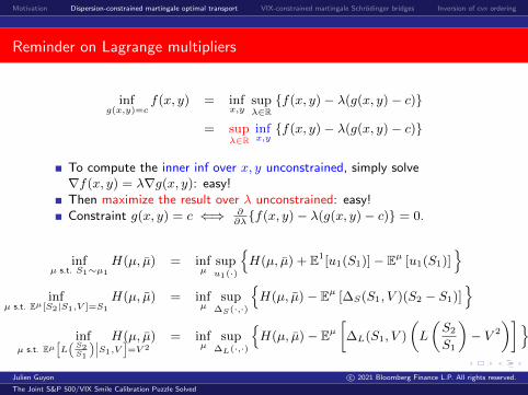
Reminder on Lagrange multipliers
infg(x,y)=c
f(x, y) = infx,y
supλ∈R{f(x, y)− λ(g(x, y)− c)}
= supλ∈R
infx,y{f(x, y)− λ(g(x, y)− c)}
To compute the inner inf over x, y unconstrained, simply solve∇f(x, y) = λ∇g(x, y): easy!Then maximize the result over λ unconstrained: easy!Constraint g(x, y) = c ⇐⇒ ∂
∂λ{f(x, y)− λ(g(x, y)− c)} = 0.
infµ s.t. S1∼µ1
H(µ, µ) = infµ
supu1(·)
{H(µ, µ) + E1[u1(S1)]− Eµ [u1(S1)]
}inf
µ s.t. Eµ[S2|S1,V ]=S1
H(µ, µ) = infµ
sup∆S(·,·)
{H(µ, µ)− Eµ [∆S(S1, V )(S2 − S1)]
}inf
µ s.t. Eµ[L(S2S1
)∣∣∣S1,V]=V 2
H(µ, µ) = infµ
sup∆L(·,·)
{H(µ, µ)− Eµ
[∆L(S1, V )
(L
(S2
S1
)− V 2
)]}Julien Guyon c© 2021 Bloomberg Finance L.P. All rights reserved.
The Joint S&P 500/VIX Smile Calibration Puzzle Solved

Motivation Dispersion-constrained martingale optimal transport VIX-constrained martingale Schrodinger bridges Inversion of cvx ordering
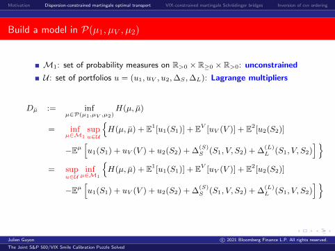
Build a model in P(µ1, µV , µ2)
M1: set of probability measures on R>0 × R≥0 × R>0: unconstrained
U : set of portfolios u = (u1, uV , u2,∆S ,∆L): Lagrange multipliers
Dµ := infµ∈P(µ1,µV ,µ2)
H(µ, µ)
= infµ∈M1
supu∈U
{H(µ, µ) + E1[u1(S1)] + EV [uV (V )] + E2[u2(S2)]
−Eµ[u1(S1) + uV (V ) + u2(S2) + ∆
(S)S (S1, V, S2) + ∆
(L)L (S1, V, S2)
]}= sup
u∈Uinf
µ∈M1
{H(µ, µ) + E1[u1(S1)] + EV [uV (V )] + E2[u2(S2)]
−Eµ[u1(S1) + uV (V ) + u2(S2) + ∆
(S)S (S1, V, S2) + ∆
(L)L (S1, V, S2)
]}
Julien Guyon c© 2021 Bloomberg Finance L.P. All rights reserved.
The Joint S&P 500/VIX Smile Calibration Puzzle Solved

Motivation Dispersion-constrained martingale optimal transport VIX-constrained martingale Schrodinger bridges Inversion of cvx ordering
Build a model in P(µ1, µV , µ2)
M1: set of probability measures on R>0 × R≥0 × R>0: unconstrained
U : set of portfolios u = (u1, uV , u2,∆S ,∆L): Lagrange multipliers
Dµ := infµ∈P(µ1,µV ,µ2)
H(µ, µ)
= infµ∈M1
supu∈U
{H(µ, µ) + E1[u1(S1)] + EV [uV (V )] + E2[u2(S2)]
−Eµ[u1(S1) + uV (V ) + u2(S2) + ∆
(S)S (S1, V, S2) + ∆
(L)L (S1, V, S2)
]}= sup
u∈Uinf
µ∈M1
{H(µ, µ) + E1[u1(S1)] + EV [uV (V )] + E2[u2(S2)]
−Eµ[u1(S1) + uV (V ) + u2(S2) + ∆
(S)S (S1, V, S2) + ∆
(L)L (S1, V, S2)
]}
Julien Guyon c© 2021 Bloomberg Finance L.P. All rights reserved.
The Joint S&P 500/VIX Smile Calibration Puzzle Solved

Motivation Dispersion-constrained martingale optimal transport VIX-constrained martingale Schrodinger bridges Inversion of cvx ordering
Build a model in P(µ1, µV , µ2)
Dµ = supu∈U
infµ∈M1
{H(µ, µ) + E1[u1(S1)] + EV [uV (V )] + E2[u2(S2)]
−Eµ[u1(S1) + uV (V ) + u2(S2) + ∆
(S)S (S1, V, S2) + ∆
(L)L (S1, V, S2)
]}
Remarkable fact: The inner infimum can be exactly computed:
infµ∈M1
{H(µ, µ)− Eµ[X]} = − lnEµ[eX]
and the infimum is attained at µ = µX defined by (Gibbs type)
dµXdµ
=eX
Eµ[eX ].
That is why we like (and chose) the “distance” H(µ, µ)!
Julien Guyon c© 2021 Bloomberg Finance L.P. All rights reserved.
The Joint S&P 500/VIX Smile Calibration Puzzle Solved

Motivation Dispersion-constrained martingale optimal transport VIX-constrained martingale Schrodinger bridges Inversion of cvx ordering
Build a model in P(µ1, µV , µ2)
Dµ := infµ∈P(µ1,µV ,µ2)
H(µ, µ) = supu∈U
Ψµ(u) =: Pµ
Ψµ(u) := E1[u1(S1)] + EV [uV (V )] + E2[u2(S2)]
− lnEµ[eu1(S1)+uV (V )+u2(S2)+∆
(S)S
(S1,V,S2)+∆(L)L
(S1,V,S2)
].
infµ∈P(µ1,µV ,µ2): constrained optimization, difficult.
supu∈U : unconstrained optimization, easy! To find the optimumu∗ = (u∗1, u
∗V , u
∗2,∆
∗S ,∆
∗L), simply cancel the gradient of Ψµ.
Most important, infµ∈P(µ1,µV ,µ2) H(µ, µ) is reached at
µ∗(ds1, dv, ds2) = µ(ds1, dv, ds2)eu∗1(s1)+u∗V (v)+u∗2(s2)+∆
∗(S)S
(s1,v,s2)+∆∗(L)L
(s1,v,s2)
Eµ[eu∗1(S1)+u∗
V(V )+u∗2(S2)+∆
∗(S)S
(S1,V,S2)+∆∗(L)L
(S1,V,S2)] .
Problem solved: µ∗ ∈ P(µ1, µV , µ2)!
Julien Guyon c© 2021 Bloomberg Finance L.P. All rights reserved.
The Joint S&P 500/VIX Smile Calibration Puzzle Solved

Motivation Dispersion-constrained martingale optimal transport VIX-constrained martingale Schrodinger bridges Inversion of cvx ordering
Minimum entropy strong duality theorem
Theorem (G. 2020)
Let µ ∈M1. Then
Dµ := infµ∈P(µ1,µV ,µ2)
H(µ, µ) = supu∈U
Ψµ(u) =: Pµ
where u = (u1, uV , u2,∆S ,∆L) and
Ψµ(u) := E1[u1(S1)] + EV [uV (V )] + E2[u2(S2)]
− lnEµ[eu1(S1)+uV (V )+u2(S2)+∆S(S1,V )(S2−S1)+∆L(S1,V )
(L(S2S1
)−V 2
)].
Moreover, when P(µ1, µV , µ2) 6= ∅, the infimum is attained. This is inparticular the case when the above quantity is finite.
Julien Guyon c© 2021 Bloomberg Finance L.P. All rights reserved.
The Joint S&P 500/VIX Smile Calibration Puzzle Solved
Motivation Dispersion-constrained martingale optimal transport VIX-constrained martingale Schrodinger bridges Inversion of cvx ordering
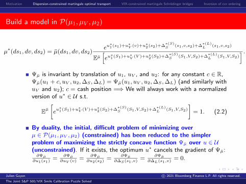
Build a model in P(µ1, µV , µ2)
µ∗(ds1, dv, ds2) = µ(ds1, dv, ds2)eu∗1(s1)+u∗V (v)+u∗2(s2)+∆
∗(S)S
(s1,v,s2)+∆∗(L)L
(s1,v,s2)
Eµ[eu∗1(S1)+u∗
V(V )+u∗2(S2)+∆
∗(S)S
(S1,V,S2)+∆∗(L)L
(S1,V,S2)] .
Ψµ is invariant by translation of u1, uV , and u2: for any constant c ∈ R,Ψµ(u1 + c, uV , u2,∆S ,∆L) = Ψµ(u1, uV , u2,∆S ,∆L) (and similarly withuV and u2); c = cash position =⇒ We will always work with a normalizedversion of u∗ ∈ U s.t.
Eµ[eu∗1(S1)+u∗V (V )+u∗2(S2)+∆
∗(S)S
(S1,V,S2)+∆∗(L)L
(S1,V,S2)
]= 1. (2.2)
By duality, the initial, difficult problem of minimizing overµ ∈ P(µ1, µV , µ2) (constrained) has been reduced to the simplerproblem of maximizing the strictly concave function Ψµ over u ∈ U(unconstrained). If it exists, the optimum u∗ cancels the gradient of Ψµ:∂Ψµ
∂u1(s1)=
∂Ψµ∂uV (v)
=∂Ψµ
∂u2(s2)=
∂Ψµ∂∆S(s1,v)
=∂Ψµ
∂∆L(s1,v)= 0.
Julien Guyon c© 2021 Bloomberg Finance L.P. All rights reserved.
The Joint S&P 500/VIX Smile Calibration Puzzle Solved

Motivation Dispersion-constrained martingale optimal transport VIX-constrained martingale Schrodinger bridges Inversion of cvx ordering
Equations for u∗ = (u∗1, u∗V , u
∗2,∆
∗S ,∆
∗L)
∂Ψµ∂u1(s1)
=0 : ∀s1 > 0, u1(s1) = Φ1(s1;uV , u2,∆S ,∆L)
∂Ψµ∂uV (v)
=0 : ∀v ≥ 0, uV (v) = ΦV (v;u1, u2,∆S ,∆L)
∂Ψµ∂u2(s2)
=0 : ∀s2 > 0, u2(s2) = Φ2(s2;u1, uV ,∆S ,∆L)
∂Ψµ∂∆S(s1,v)
=0 : ∀s1 > 0, ∀v ≥ 0, 0 = Φ∆S (s1, v; ∆S(s1, v),∆L(s1, v))
∂Ψµ∂∆L(s1,v)
=0 : ∀s1 > 0, ∀v ≥ 0, 0 = Φ∆L(s1, v; ∆S(s1, v),∆L(s1, v))
We could have simply postulated a model of the form
µ(ds1, dv, ds2) = µ(ds1, dv, ds2)eu1(s1)+uV (v)+u2(s2)+∆
(S)S
(s1,v,s2)+∆(L)L
(s1,v,s2)
Eµ[eu1(S1)+uV (V )+u2(S2)+∆
(S)S
(S1,V,S2)+∆(L)L
(S1,V,S2)] .
Then the 5 conditions defining P(µ1, µV , µ2) translate into the 5 aboveequations.
The system of equations is solved using Sinkhorn’s algorithm.
If the algorithm diverges, then Pµ = +∞, so Dµ = +∞, i.e.,P(µ1, µV , µ2) ∩ {µ ∈M1|µ� µ} = ∅. In practice, when µ has fullsupport, this is a sign that there likely exists a joint SPX/VIX arbitrage.
Julien Guyon c© 2021 Bloomberg Finance L.P. All rights reserved.
The Joint S&P 500/VIX Smile Calibration Puzzle Solved

Motivation Dispersion-constrained martingale optimal transport VIX-constrained martingale Schrodinger bridges Inversion of cvx ordering
Sinkhorn’s algorithm
Sinkhorn’s algorithm (1967) was first used in the context of optimaltransport by Cuturi (2013).
In our context: fixed point method that iterates computions ofone-dimensional gradients to approximate the optimizer u∗.
Start from initial guess u(0) = (u(0)1 , u
(0)V , u
(0)2 ,∆
(0)S ,∆
(0)L ), recursively
define u(n+1) knowing u(n) by
∀s1 > 0, u(n+1)1 (s1) = Φ1(s1;u
(n)V , u
(n)2 ,∆
(n)S ,∆
(n)L )
∀v ≥ 0, u(n+1)V (v) = ΦV (v;u
(n+1)1 , u
(n)2 ,∆
(n)S ,∆
(n)L )
∀s2 > 0, u(n+1)2 (s2) = Φ2(s2;u
(n+1)1 , u
(n+1)V ,∆
(n)S ,∆
(n)L )
∀s1 > 0, ∀v ≥ 0, 0 = Φ∆S (s1, v;u(n+1)2 ,∆
(n+1)S (s1, v),∆
(n)L (s1, v))
∀s1 > 0, ∀v ≥ 0, 0 = Φ∆L(s1, v;u(n+1)2 ,∆
(n+1)S (s1, v),∆
(n+1)L (s1, v))
until convergence.
Each of the above 5 lines corresponds to a Bregman projection in thespace of measures.
Julien Guyon c© 2021 Bloomberg Finance L.P. All rights reserved.
The Joint S&P 500/VIX Smile Calibration Puzzle Solved

Motivation Dispersion-constrained martingale optimal transport VIX-constrained martingale Schrodinger bridges Inversion of cvx ordering
Sinkhorn’s algorithm
Sinkhorn’s algorithm (1967) was first used in the context of optimaltransport by Cuturi (2013).In our context: fixed point method that iterates computions ofone-dimensional gradients to approximate the optimizer u∗.Start from initial guess u(0) = (u
(0)1 , u
(0)V , u
(0)2 ,∆
(0)S ,∆
(0)L ), recursively
define u(n+1) knowing u(n) by
∀s1 > 0, u(n+1)1 (s1) = Φ1(s1;u
(n)V , u
(n)2 ,∆
(n)S ,∆
(n)L )
∀v ≥ 0, u(n+1)V (v) = ΦV (v;u
(n+1)1 , u
(n)2 ,∆
(n)S ,∆
(n)L )
∀s2 > 0, u(n+1)2 (s2) = Φ2(s2;u
(n+1)1 , u
(n+1)V ,∆
(n)S ,∆
(n)L )
∀s1 > 0, ∀v ≥ 0, 0 = Φ∆S (s1, v;u(n+1)2 ,∆
(n+1)S (s1, v),∆
(n)L (s1, v))
∀s1 > 0, ∀v ≥ 0, 0 = Φ∆L(s1, v;u(n+1)2 ,∆
(n+1)S (s1, v),∆
(n+1)L (s1, v))
Each of the above five lines corresponds to a Bregman projection in thespace of measures.If the algorithm diverges, then Pµ = +∞, so Dµ = +∞, i.e.,P(µ1, µV , µ2) ∩ {µ ∈M1|µ� µ} = ∅. In practice, when µ has fullsupport, this is a sign that there likely exists a joint SPX/VIX arbitrage.
Julien Guyon c© 2021 Bloomberg Finance L.P. All rights reserved.
The Joint S&P 500/VIX Smile Calibration Puzzle Solved

Motivation Dispersion-constrained martingale optimal transport VIX-constrained martingale Schrodinger bridges Inversion of cvx ordering
Numerical experiments
Julien Guyon c© 2021 Bloomberg Finance L.P. All rights reserved.
The Joint S&P 500/VIX Smile Calibration Puzzle Solved

Motivation Dispersion-constrained martingale optimal transport VIX-constrained martingale Schrodinger bridges Inversion of cvx ordering
Implementation details
Choice of µ:S1 ∼ µ1 and V ∼ µV independent;Conditional on (S1, V ), S2 lognormal with mean S1 and variance V .
Under µ, S2 6∼ µ2.
Instead of abstract payoffs u1, uV , u2, we work with market strikes andmarket prices of vanilla options on S1, V , and S2.
Canceling the gradient of Ψµ → system of equations solved usingSinkhorn’s algorithm.
Enough accuracy is typically reached after ≈ 100 iterations.
Julien Guyon c© 2021 Bloomberg Finance L.P. All rights reserved.
The Joint S&P 500/VIX Smile Calibration Puzzle Solved

Motivation Dispersion-constrained martingale optimal transport VIX-constrained martingale Schrodinger bridges Inversion of cvx ordering
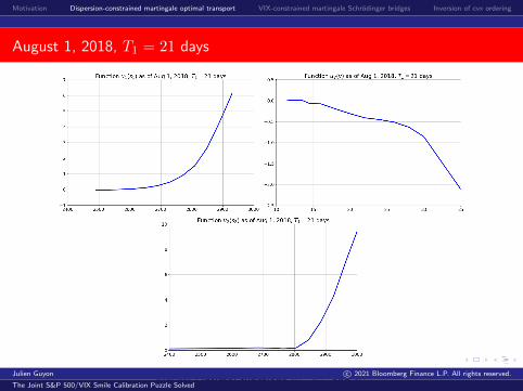
August 1, 2018, T1 = 21 days
Julien Guyon c© 2021 Bloomberg Finance L.P. All rights reserved.
The Joint S&P 500/VIX Smile Calibration Puzzle Solved

Motivation Dispersion-constrained martingale optimal transport VIX-constrained martingale Schrodinger bridges Inversion of cvx ordering
August 1, 2018, T1 = 21 days
Julien Guyon c© 2021 Bloomberg Finance L.P. All rights reserved.
The Joint S&P 500/VIX Smile Calibration Puzzle Solved

Motivation Dispersion-constrained martingale optimal transport VIX-constrained martingale Schrodinger bridges Inversion of cvx ordering
August 1, 2018, T1 = 21 days
Figure: Joint distribution of (S1, V ) and local VIX function VIXloc(s1)
VIX2loc(S1) := Eµ
∗ [V 2∣∣S1
]Julien Guyon c© 2021 Bloomberg Finance L.P. All rights reserved.
The Joint S&P 500/VIX Smile Calibration Puzzle Solved

Motivation Dispersion-constrained martingale optimal transport VIX-constrained martingale Schrodinger bridges Inversion of cvx ordering
August 1, 2018, T1 = 21 days
4 3 2 1 0 1 2 3 40.0
0.1
0.2
0.3
0.4
0.5
0.6
0.7
0.8 Distribution of lnS2S1
V + 12V , calib as of Aug 1, 2018, T1 = 21 days
Figure: Conditional distribution of S2 given (s1, v) under µ∗ for different vales of(s1, v): s1 ∈ {2571, 2808, 3000}, v ∈ {10.10, 15.30, 23.20, 35.72}%, and distribution
of the normalized return R :=ln(S2/S1)
V√τ
+ 12V√τ
Julien Guyon c© 2021 Bloomberg Finance L.P. All rights reserved.
The Joint S&P 500/VIX Smile Calibration Puzzle Solved
Motivation Dispersion-constrained martingale optimal transport VIX-constrained martingale Schrodinger bridges Inversion of cvx ordering
August 1, 2018, T1 = 21 days
Figure: Optimal functions u∗1, u∗V and u∗2Julien Guyon c© 2021 Bloomberg Finance L.P. All rights reserved.
The Joint S&P 500/VIX Smile Calibration Puzzle Solved

Motivation Dispersion-constrained martingale optimal transport VIX-constrained martingale Schrodinger bridges Inversion of cvx ordering
August 1, 2018, T1 = 21 days
Figure: Optimal functions ∆∗S(s1, v) and ∆∗L(s1, v) for (s1, v) in the quadrature grid
Julien Guyon c© 2021 Bloomberg Finance L.P. All rights reserved.
The Joint S&P 500/VIX Smile Calibration Puzzle Solved

Motivation Dispersion-constrained martingale optimal transport VIX-constrained martingale Schrodinger bridges Inversion of cvx ordering
August 1, 2018, T1 = 49 days
Julien Guyon c© 2021 Bloomberg Finance L.P. All rights reserved.
The Joint S&P 500/VIX Smile Calibration Puzzle Solved

Motivation Dispersion-constrained martingale optimal transport VIX-constrained martingale Schrodinger bridges Inversion of cvx ordering
August 1, 2018, T1 = 49 days
Julien Guyon c© 2021 Bloomberg Finance L.P. All rights reserved.
The Joint S&P 500/VIX Smile Calibration Puzzle Solved

Motivation Dispersion-constrained martingale optimal transport VIX-constrained martingale Schrodinger bridges Inversion of cvx ordering
December 24, 2018, T1 = 23 days: large VIX, FV ≈ 26%
Julien Guyon c© 2021 Bloomberg Finance L.P. All rights reserved.
The Joint S&P 500/VIX Smile Calibration Puzzle Solved

Motivation Dispersion-constrained martingale optimal transport VIX-constrained martingale Schrodinger bridges Inversion of cvx ordering
December 24, 2018, T1 = 23 days
Julien Guyon c© 2021 Bloomberg Finance L.P. All rights reserved.
The Joint S&P 500/VIX Smile Calibration Puzzle Solved

Motivation Dispersion-constrained martingale optimal transport VIX-constrained martingale Schrodinger bridges Inversion of cvx ordering
MOT in continuous time:Exact joint calibration via
VIX-constrained martingaleSchrodinger bridges
(G. 2020)
Julien Guyon c© 2021 Bloomberg Finance L.P. All rights reserved.
The Joint S&P 500/VIX Smile Calibration Puzzle Solved

Motivation Dispersion-constrained martingale optimal transport VIX-constrained martingale Schrodinger bridges Inversion of cvx ordering
Martingale optimal transport approach in continuous time
Same point of view as the discrete-time model: Pick a reference measureP0 ←→ a particular SV model:
dStSt
= at dW0t
dat = b(at) dt+ σ(at)(ρ dW 0
t +√
1− ρ2dW 0,⊥t
)We want to prove that P 6= ∅ and build P ∈ P, where
P := {P� P0|S1 ∼ µ1, S2 ∼ µ2,√
EP[L(S2/S1)|F1] ∼ µV , S is a P-martingale}.
No need to introduce a new r.v. for the VIX: VIX =√
EP[L(S2/S1)|F1].
We look for P ∈ P that minimizes the relative entropy w.r.t. P0:
D := infP∈P
H(P,P0)
Inspired by Henry-Labordere 2019: From (Martingale) Schrodinger Bridgesto a New Class of Stochastic Volatility Models (calib to SPX smiles)
Follows closely the construction of Schrodinger bridges
Julien Guyon c© 2021 Bloomberg Finance L.P. All rights reserved.
The Joint S&P 500/VIX Smile Calibration Puzzle Solved

Motivation Dispersion-constrained martingale optimal transport VIX-constrained martingale Schrodinger bridges Inversion of cvx ordering
Simple Schrodinger bridge (a la Follmer, Saint-Flour 1988)
dXt = dW 0t , X0 = x0
P := {P� P0 |X1 ∼ µ1}
D := infP∈P
H(P,P0)
= infP∈M1
supu1∈L1(µ1)
{H(P,P0) + Eµ1 [u1(X1)]− EP [u1(X1)]
}= sup
u1∈L1(µ1)
infP∈M1
{H(P,P0) + Eµ1 [u1(X1)]− EP [u1(X1)]
}Recall the remarkable fact about the inner infimum:
infP∈M1
{H(P,P0)− EP [u1(X1)]
}= − lnEP0
[eu1(X1)
]and the infimum is reached at P∗ defined by
dP∗
dP0=
eu1(X1)
EP0 [eu1(X1)].
Julien Guyon c© 2021 Bloomberg Finance L.P. All rights reserved.
The Joint S&P 500/VIX Smile Calibration Puzzle Solved

Motivation Dispersion-constrained martingale optimal transport VIX-constrained martingale Schrodinger bridges Inversion of cvx ordering
Simple Schrodinger bridge (a la Follmer, Saint-Flour 1988)
dXt = dW 0t , X0 = x0
P := {P� P0 |X1 ∼ µ1}
D := infP∈P
H(P,P0)
= infP∈M1
supu1∈L1(µ1)
{H(P,P0) + Eµ1 [u1(X1)]− EP [u1(X1)]
}= sup
u1∈L1(µ1)
infP∈M1
{H(P,P0) + Eµ1 [u1(X1)]−EP [u1(X1)]
}Recall the remarkable fact about the inner infimum:
infP∈M1
{H(P,P0)− EP [u1(X1)]
}= − lnEP0
[eu1(X1)
]and the infimum is reached at P∗ defined by
dP∗
dP0=
eu1(X1)
EP0 [eu1(X1)].
Julien Guyon c© 2021 Bloomberg Finance L.P. All rights reserved.
The Joint S&P 500/VIX Smile Calibration Puzzle Solved

Motivation Dispersion-constrained martingale optimal transport VIX-constrained martingale Schrodinger bridges Inversion of cvx ordering
Simple Schrodinger bridge (a la Follmer, Saint-Flour 1988)
D := infP∈P
H(P,P0) = supu1∈L1(µ1)
{Eµ1 [u1(X1)]− lnEP0
[eu1(X1)
]}=: P
Assume P < +∞ and the sup is reached at u∗1. Then
MT1 :=dP∗
dP0= eu
∗1(X1) (Z = 1 by cash adjustment of u∗1)
Let Mt := EP0 [MT1 |Ft] = EP0 [eu∗1(X1)|Ft]. Then Mt = U∗(t,Xt) where
∂tU∗ +
1
2∂2xU∗ = 0, U∗(T1, x) = eu
∗1(x).
By Girsanov, W ∗t := W 0t −
∫ t0∂x lnU∗(s,Xs) ds is a P∗-Brownian motion,
dXt = ∂x lnU∗(t,Xt) dt+ dW ∗t = ∂x lnEP0 [eu∗1(X1)|Xt = x]|Xt dt+ dW ∗t
Brownian motion with drift, which is explicitly known.In practice, u1(X1) is replaced by
∑K∈K αK(X1 −K)+. The gradient of
Eµ1
[∑K∈K
αK(X1 −K)+
]− lnEP0
[e∑K∈K αK(X1−K)+
]is simply the vector of differences between model and market call prices.
Julien Guyon c© 2021 Bloomberg Finance L.P. All rights reserved.
The Joint S&P 500/VIX Smile Calibration Puzzle Solved
Motivation Dispersion-constrained martingale optimal transport VIX-constrained martingale Schrodinger bridges Inversion of cvx ordering
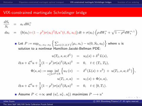
VIX-constrained martingale Schrodinger bridge
dStSt
= at dW∗t
dat =(b(at)+(1− ρ2)σ(at)
2∂au∗(t, St, at)
)dt+ σ(at)
(ρ dW ∗t +
√1− ρ2dW ∗,⊥t
)Let P := supu1,uV ,u2
{∑i∈{1,2,V }(µi, ui)− u(0, S0, a0)
}where u is
solution to a nonlinear Hamilton-Jacobi-Bellman PDE:
u(T2, s, a; δL) = u2(s) + δLL(s),
∂tu+ L0u+1
2(1− ρ2)σ(a)2(∂au)2 = 0, t ∈ (T1, T2),
Φ(s, a) := supv≥0
infδL∈R
{uV (v) − δL(L(s) + v2) + u(T1, s, a; δL)
},
u(T1, s, a) = u1(s) + Φ(s, a),
∂tu+ L0u+1
2(1− ρ2)σ(a)2(∂au)2 = 0, t ∈ [0, T1).
Assume P < +∞ and (u∗1, u∗V , u
∗2) maximizes P −→ u∗
Julien Guyon c© 2021 Bloomberg Finance L.P. All rights reserved.
The Joint S&P 500/VIX Smile Calibration Puzzle Solved

Motivation Dispersion-constrained martingale optimal transport VIX-constrained martingale Schrodinger bridges Inversion of cvx ordering
VIX-constrained martingale Schrodinger bridge
dStSt
= at dW∗t
dat =(b(at)+(1− ρ2)σ(at)
2∂au∗(t, St, at)
)dt+ σ(at)
(ρ dW ∗t +
√1− ρ2dW ∗,⊥t
)Optimal deltas:
∆∗t = −∂su∗(t, St, at)− ρσ(at)
atSt∂au
∗(t, St, at); ∆∗,L = δ∗,L(S1, a1)
The drift of (at) under P∗ also reads as
b(at) + (1− ρ2)σ(at)2∂a lnE0[eu
∗1(S1)+
∫ T1t ∆∗(r,Sr,ar)dSr+Φ∗(S1,a1)|St, at], t ∈ [0, T1],
b(at) + (1− ρ2)σ(at)2∂a lnE0[eu
∗2(S2)+
∫ T2t ∆∗(r,Sr,ar)dSr+δ∗,L(S1,a1)L(S2)|St, at], t ∈ [T1, T2].
It is path-dependent on [T1, T2] so as to match the market VIX smile.
If P = +∞, then P = ∅.
Julien Guyon c© 2021 Bloomberg Finance L.P. All rights reserved.
The Joint S&P 500/VIX Smile Calibration Puzzle Solved

Motivation Dispersion-constrained martingale optimal transport VIX-constrained martingale Schrodinger bridges Inversion of cvx ordering
Martingale optimal transport approach in continuous time
D := infP∈P
H(P, P0)
= infP∈M1
sup
u1∈L1(µ1),u2∈L1(µ2),uV ∈L1(µV ),(∆t)F-adapted
{H(P, P0) +
∑i∈{1,2,V }
(µi, ui)
−EPu1(S1) + u2(S2) + uV
√√√√EP
[L
(S2
S1
)∣∣∣∣∣F1
] +
∫ T2
0∆tdSt
}(relax)
= infP∈M1
supu1,u2,uV ,(∆t)
infV∈F1
sup
∆L∈F1
{H(P, P0) +
∑i∈{1,2,V }
(µi, ui)
−EP[u1(S1) + u2(S2) + uV (V ) +
∫ T2
0∆tdSt + ∆
L(L
(S2
S1
)− V 2
)] }(dual)
= supu1,u2,uV ,(∆t)
infV∈F1
sup
∆L∈F1
infP∈M1
{H(P, P0) +
∑i∈{1,2,V }
(µi, ui)
−EP[u1(S1) + u2(S2) + uV (V ) +
∫ T2
0∆tdSt + ∆
L(L
(S2
S1
)− V 2
)] }= sup
u1,u2,uV ,(∆t)inf
V∈F1sup
∆L∈F1
{ ∑i∈{1,2,V }
(µi, ui)
− ln E0
eu1(S1)+u2(S2)+uV (V )+∫T20 ∆tdSt+∆L
(L
(S2S1
)−V 2
) }
= supu1,u2,uV
sup(∆t)t∈[0,T1]
infV∈F1
sup
∆L∈F1
sup(∆t)t∈[T1,T2]
{· · ·
}Julien Guyon c© 2021 Bloomberg Finance L.P. All rights reserved.
The Joint S&P 500/VIX Smile Calibration Puzzle Solved

Motivation Dispersion-constrained martingale optimal transport VIX-constrained martingale Schrodinger bridges Inversion of cvx ordering
Lagrange multipliers u1, u2, uV
D := infP∈P
H(P, P0)
= infP∈M1
sup
u1∈L1(µ1),u2∈L1(µ2),uV ∈L1(µV ),(∆t)F-adapted
{H(P, P0) +
∑i∈{1,2,V }
(µi, ui)
−EPu1(S1) + u2(S2) + uV
√√√√EP
[L
(S2
S1
)∣∣∣∣∣F1
] +
∫ T2
0∆tdSt
}(relax)
= infP∈M1
supu1,u2,uV ,(∆t)
infV∈F1
sup
∆L∈F1
{H(P, P0) +
∑i∈{1,2,V }
(µi, ui)
−EP[u1(S1) + u2(S2) + uV (V ) +
∫ T2
0∆tdSt + ∆
L(L
(S2
S1
)− V 2
)] }(dual)
= supu1,u2,uV ,(∆t)
infV∈F1
sup
∆L∈F1
infP∈M1
{H(P, P0) +
∑i∈{1,2,V }
(µi, ui)
−EP[u1(S1) + u2(S2) + uV (V ) +
∫ T2
0∆tdSt + ∆
L(L
(S2
S1
)− V 2
)] }= sup
u1,u2,uV ,(∆t)inf
V∈F1sup
∆L∈F1
{ ∑i∈{1,2,V }
(µi, ui)
− ln E0
eu1(S1)+u2(S2)+uV (V )+∫T20 ∆tdSt+∆L
(L
(S2S1
)−V 2
) }
= supu1,u2,uV
sup(∆t)t∈[0,T1]
infV∈F1
sup
∆L∈F1
sup(∆t)t∈[T1,T2]
{· · ·
}Julien Guyon c© 2021 Bloomberg Finance L.P. All rights reserved.
The Joint S&P 500/VIX Smile Calibration Puzzle Solved

Motivation Dispersion-constrained martingale optimal transport VIX-constrained martingale Schrodinger bridges Inversion of cvx ordering
Lagrange multipliers ∆t: martingality of S
D := infP∈P
H(P, P0)
= infP∈M1
sup
u1∈L1(µ1),u2∈L1(µ2),uV ∈L1(µV ),(∆t)F-adapted
{H(P, P0) +
∑i∈{1,2,V }
(µi, ui)
−EPu1(S1) + u2(S2) + uV
√√√√EP
[L
(S2
S1
)∣∣∣∣∣F1
] +
∫ T2
0∆tdSt
}(relax)
= infP∈M1
supu1,u2,uV ,(∆t)
infV∈F1
sup
∆L∈F1
{H(P, P0) +
∑i∈{1,2,V }
(µi, ui)
−EP[u1(S1) + u2(S2) + uV (V ) +
∫ T2
0∆tdSt + ∆
L(L
(S2
S1
)− V 2
)] }(dual)
= supu1,u2,uV ,(∆t)
infV∈F1
sup
∆L∈F1
infP∈M1
{H(P, P0) +
∑i∈{1,2,V }
(µi, ui)
−EP[u1(S1) + u2(S2) + uV (V ) +
∫ T2
0∆tdSt + ∆
L(L
(S2
S1
)− V 2
)] }= sup
u1,u2,uV ,(∆t)inf
V∈F1sup
∆L∈F1
{ ∑i∈{1,2,V }
(µi, ui)
− ln E0
eu1(S1)+u2(S2)+uV (V )+∫T20 ∆tdSt+∆L
(L
(S2S1
)−V 2
) }
= supu1,u2,uV
sup(∆t)t∈[0,T1]
infV∈F1
sup
∆L∈F1
sup(∆t)t∈[T1,T2]
{· · ·
}Julien Guyon c© 2021 Bloomberg Finance L.P. All rights reserved.
The Joint S&P 500/VIX Smile Calibration Puzzle Solved

Motivation Dispersion-constrained martingale optimal transport VIX-constrained martingale Schrodinger bridges Inversion of cvx ordering
Relaxation
EP
[uV
(√EP[L
(S2
S1
)∣∣∣∣F1
])]= infV ∈F1
sup∆L∈F1
EP[uV (V ) + ∆L
(L
(S2
S1
)− V 2
)]
Julien Guyon c© 2021 Bloomberg Finance L.P. All rights reserved.
The Joint S&P 500/VIX Smile Calibration Puzzle Solved

Motivation Dispersion-constrained martingale optimal transport VIX-constrained martingale Schrodinger bridges Inversion of cvx ordering
Relaxation
D := infP∈P
H(P, P0)
= infP∈M1
sup
u1∈L1(µ1),u2∈L1(µ2),uV ∈L1(µV ),(∆t)F-adapted
{H(P, P0) +
∑i∈{1,2,V }
(µi, ui)
−EPu1(S1) + u2(S2) + uV
√√√√EP
[L
(S2
S1
)∣∣∣∣∣F1
] +
∫ T2
0∆tdSt
}(relax)
= infP∈M1
supu1,u2,uV ,(∆t)
infV∈F1
sup
∆L∈F1
{H(P, P0) +
∑i∈{1,2,V }
(µi, ui)
−EP[u1(S1) + u2(S2) + uV (V ) +
∫ T2
0∆tdSt + ∆
L(L
(S2
S1
)− V 2
)] }(dual)
= supu1,u2,uV ,(∆t)
infV∈F1
sup
∆L∈F1
infP∈M1
{H(P, P0) +
∑i∈{1,2,V }
(µi, ui)
−EP[u1(S1) + u2(S2) + uV (V ) +
∫ T2
0∆tdSt + ∆
L(L
(S2
S1
)− V 2
)] }= sup
u1,u2,uV ,(∆t)inf
V∈F1sup
∆L∈F1
{ ∑i∈{1,2,V }
(µi, ui)
− ln E0
eu1(S1)+u2(S2)+uV (V )+∫T20 ∆tdSt+∆L
(L
(S2S1
)−V 2
) }
= supu1,u2,uV
sup(∆t)t∈[0,T1]
infV∈F1
sup
∆L∈F1
sup(∆t)t∈[T1,T2]
{· · ·
}Julien Guyon c© 2021 Bloomberg Finance L.P. All rights reserved.
The Joint S&P 500/VIX Smile Calibration Puzzle Solved

Motivation Dispersion-constrained martingale optimal transport VIX-constrained martingale Schrodinger bridges Inversion of cvx ordering
Duality
D := infP∈P
H(P, P0)
= infP∈M1
sup
u1∈L1(µ1),u2∈L1(µ2),uV ∈L1(µV ),(∆t)F-adapted
{H(P, P0) +
∑i∈{1,2,V }
(µi, ui)
−EPu1(S1) + u2(S2) + uV
√√√√EP
[L
(S2
S1
)∣∣∣∣∣F1
] +
∫ T2
0∆tdSt
}(relax)
= infP∈M1
supu1,u2,uV ,(∆t)
infV∈F1
sup
∆L∈F1
{H(P, P0) +
∑i∈{1,2,V }
(µi, ui)
−EP[u1(S1) + u2(S2) + uV (V ) +
∫ T2
0∆tdSt + ∆
L(L
(S2
S1
)− V 2
)] }(dual)
= supu1,u2,uV ,(∆t)
infV∈F1
sup
∆L∈F1
infP∈M1
{H(P, P0) +
∑i∈{1,2,V }
(µi, ui)
−EP[u1(S1) + u2(S2) + uV (V ) +
∫ T2
0∆tdSt + ∆
L(L
(S2
S1
)− V 2
)] }= sup
u1,u2,uV ,(∆t)inf
V∈F1sup
∆L∈F1
{ ∑i∈{1,2,V }
(µi, ui)
− ln E0
eu1(S1)+u2(S2)+uV (V )+∫T20 ∆tdSt+∆L
(L
(S2S1
)−V 2
) }
= supu1,u2,uV
sup(∆t)t∈[0,T1]
infV∈F1
sup
∆L∈F1
sup(∆t)t∈[T1,T2]
{· · ·
}Julien Guyon c© 2021 Bloomberg Finance L.P. All rights reserved.
The Joint S&P 500/VIX Smile Calibration Puzzle Solved

Motivation Dispersion-constrained martingale optimal transport VIX-constrained martingale Schrodinger bridges Inversion of cvx ordering
Remarkable fact: inner inf is explicit
D := infP∈P
H(P, P0)
= infP∈M1
sup
u1∈L1(µ1),u2∈L1(µ2),uV ∈L1(µV ),(∆t)F-adapted
{H(P, P0) +
∑i∈{1,2,V }
(µi, ui)
−EPu1(S1) + u2(S2) + uV
√√√√EP
[L
(S2
S1
)∣∣∣∣∣F1
] +
∫ T2
0∆tdSt
}(relax)
= infP∈M1
supu1,u2,uV ,(∆t)
infV∈F1
sup
∆L∈F1
{H(P, P0) +
∑i∈{1,2,V }
(µi, ui)
−EP[u1(S1) + u2(S2) + uV (V ) +
∫ T2
0∆tdSt + ∆
L(L
(S2
S1
)− V 2
)] }(dual)
= supu1,u2,uV ,(∆t)
infV∈F1
sup
∆L∈F1
infP∈M1
{H(P, P0) +
∑i∈{1,2,V }
(µi, ui)
−EP[u1(S1) + u2(S2) + uV (V ) +
∫ T2
0∆tdSt + ∆
L(L
(S2
S1
)− V 2
)]}= sup
u1,u2,uV ,(∆t)inf
V∈F1sup
∆L∈F1
{ ∑i∈{1,2,V }
(µi, ui)
− ln E0
eu1(S1)+u2(S2)+uV (V )+∫T20 ∆tdSt+∆L
(L
(S2S1
)−V 2
)}
= supu1,u2,uV
sup(∆t)t∈[0,T1]
infV∈F1
sup
∆L∈F1
sup(∆t)t∈[T1,T2]
{· · ·
}Julien Guyon c© 2021 Bloomberg Finance L.P. All rights reserved.
The Joint S&P 500/VIX Smile Calibration Puzzle Solved

Motivation Dispersion-constrained martingale optimal transport VIX-constrained martingale Schrodinger bridges Inversion of cvx ordering
Optimizing first over [T1, T2], then T1, then [T0, T1], then T0
D := infP∈P
H(P, P0)
= infP∈M1
sup
u1∈L1(µ1),u2∈L1(µ2),uV ∈L1(µV ),(∆t)F-adapted
{H(P, P0) +
∑i∈{1,2,V }
(µi, ui)
−EPu1(S1) + u2(S2) + uV
√√√√EP
[L
(S2
S1
)∣∣∣∣∣F1
] +
∫ T2
0∆tdSt
}(relax)
= infP∈M1
supu1,u2,uV ,(∆t)
infV∈F1
sup
∆L∈F1
{H(P, P0) +
∑i∈{1,2,V }
(µi, ui)
−EP[u1(S1) + u2(S2) + uV (V ) +
∫ T2
0∆tdSt + ∆
L(L
(S2
S1
)− V 2
)] }(dual)
= supu1,u2,uV ,(∆t)
infV∈F1
sup
∆L∈F1
infP∈M1
{H(P, P0) +
∑i∈{1,2,V }
(µi, ui)
−EP[u1(S1) + u2(S2) + uV (V ) +
∫ T2
0∆tdSt + ∆
L(L
(S2
S1
)− V 2
)] }= sup
u1,u2,uV ,(∆t)inf
V∈F1sup
∆L∈F1
{ ∑i∈{1,2,V }
(µi, ui)
− ln E0
eu1(S1)+u2(S2)+uV (V )+∫T20 ∆tdSt+∆L
(L
(S2S1
)−V 2
) }
= supu1,u2,uV
sup(∆t)t∈[0,T1]
infV∈F1
sup
∆L∈F1
sup(∆t)t∈[T1,T2]
{· · ·
}Julien Guyon c© 2021 Bloomberg Finance L.P. All rights reserved.
The Joint S&P 500/VIX Smile Calibration Puzzle Solved

Motivation Dispersion-constrained martingale optimal transport VIX-constrained martingale Schrodinger bridges Inversion of cvx ordering
Optimize over [T1, T2]
The inner infP∈M1 is reached at P∗ defined by (renorm. Z = 1 by cashadjustment of vanilla payoffs)
dP∗
dP0= e
u1(S1)+u2(S2)+uV (V )+∫ T20 ∆tdSt+∆L
(L(S2S1
)−V 2
)
D = supu1,u2,uV
sup(∆t)t∈[0,T1]
infV∈F1
sup
∆L∈F1
sup(∆t)t∈[T1,T2]
{ ∑i∈{1,2,V }
(µi, ui)
− ln E0
eu1(S1)+u2(S2)+uV (V )+∫T20 ∆tdSt+∆L
(L
(S2S1
)−V 2
) }
= supu1,u2,uV
sup(∆t)t∈[0,T1]
infV∈F1
sup
∆L∈F1
{ ∑i∈{1,2,V }
(µi, ui)
− ln inf(∆t)t∈[T1,T2]
E0
eu1(S1)+u2(S2)+uV (V )+∫T20 ∆tdSt+∆L
(L
(S2S1
)−V 2
) }
Julien Guyon c© 2021 Bloomberg Finance L.P. All rights reserved.
The Joint S&P 500/VIX Smile Calibration Puzzle Solved

Motivation Dispersion-constrained martingale optimal transport VIX-constrained martingale Schrodinger bridges Inversion of cvx ordering
Optimize over [T1, T2]: stochastic control
D = supu1,u2,uV
sup(∆t)t∈[0,T1]
infV∈F1
sup
∆L∈F1
{ ∑i∈{1,2,V }
(µi, ui)
− ln inf(∆t)t∈[T1,T2]
E0
eu1(S1)+u2(S2)+uV (V )+∫T20 ∆tdSt+∆L
(L
(S2S1
)−V 2
)}(DPP)
= supu1,u2,uV
sup(∆t)t∈[0,T1]
infV∈F1
sup
∆L∈F1
{ ∑i∈{1,2,V }
(µi, ui)
− ln E0
eu1(S1)+uV (V )+∫T10 ∆tdSt−∆L(L(S1)+V 2)
U(T1, S1, a1; ∆L
)
}
Stochastic control:
U(t, St, at; ∆L) := inf(∆r)r∈[t,T2]
E0
[eu2(S2)+
∫ T2t ∆rdSr+∆LL(S2)
∣∣∣∣St, at,∆L
], t ∈ [T1, T2].
Julien Guyon c© 2021 Bloomberg Finance L.P. All rights reserved.
The Joint S&P 500/VIX Smile Calibration Puzzle Solved

Motivation Dispersion-constrained martingale optimal transport VIX-constrained martingale Schrodinger bridges Inversion of cvx ordering
Optimize over [T1, T2]: stochastic control
U is solution to the HJB PDE
∂tU + L0U + inf∆
{1
2∆2a2s2U + ∆as (as∂sU + ρσ(a)∂aU)
}= 0,
U(T2, s, a; δL) = eu2(s)+δLL(s).
Optimal delta:
∆∗t = −∂sU(t, St, at) + ρσ(at)
atSt∂aU(t, St, at)
U(t, St, at),
U satisfies
∂tU+L0U− (as∂sU + ρσ(a)∂aU)2
2U= 0, U(T2, s, a; δL) = eu2(s)+δLL(s).
u := lnU satisfies
∂tu+ L0u+1
2(1− ρ2)σ(a)2(∂au)2 = 0, u(T2, s, a; δL) = u2(s) + δLL(s).
Julien Guyon c© 2021 Bloomberg Finance L.P. All rights reserved.
The Joint S&P 500/VIX Smile Calibration Puzzle Solved

Motivation Dispersion-constrained martingale optimal transport VIX-constrained martingale Schrodinger bridges Inversion of cvx ordering
Optimize at T1: simply pathwise
D = supu1,u2,uV
sup(∆t)t∈[0,T1]
infV ∈F1
sup∆L∈F1
{ ∑i∈{1,2,V }
(µi, ui)
− lnE0
[eu1(S1)+uV (V )+
∫ T10 ∆tdSt−∆L(L(S1)+V 2)+u(T1,S1,a1;∆L)
]}Since S1, a1, and
∫ T1
0∆tdSt are F1-measurable,
infV ∈F1
sup∆L∈F1
{− lnE0
[eu1(S1)+uV (V )+
∫ T10 ∆tdSt−∆L(L(S1)+V 2)+u(T1,S1,a1;∆L)
]}= − ln sup
V ∈F1
inf∆L∈F1
E0
[eu1(S1)+uV (V )+
∫ T10 ∆tdSt−∆L(L(S1)+V 2)+u(T1,S1,a1;∆L)
]= − lnE0
[eu1(S1)+
∫ T10 ∆tdSt+Φ(S1,a1)
]Φ(s, a) := sup
v≥0infδL∈R
{uV (v)− δL(L(s) + v2) + u(T1, s, a; δL)
}.
The optimal V and ∆L are functions of (S1, a1): v∗(S1, a1), δ∗L(S1, a1).
Julien Guyon c© 2021 Bloomberg Finance L.P. All rights reserved.
The Joint S&P 500/VIX Smile Calibration Puzzle Solved

Motivation Dispersion-constrained martingale optimal transport VIX-constrained martingale Schrodinger bridges Inversion of cvx ordering
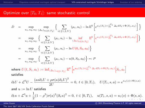
Optimize over [T0, T1]: same stochastic control
D = supu1,u2,uV
sup(∆t)t∈[0,T1]
{ ∑i∈{1,2,V }
(µi, ui) − ln E0
[eu1(S1)+
∫ T10 ∆tdSt+Φ(S1,a1)
]}= sup
u1,u2,uV
{ ∑i∈{1,2,V }
(µi, ui) − ln inf(∆t)t∈[0,T1]
E0
[eu1(S1)+
∫ T10 ∆tdSt+Φ(S1,a1)
]}= sup
u1,u2,uV
{ ∑i∈{1,2,V }
(µi, ui)− lnU(0, S0, a0)}
= supu1,u2,uV
{ ∑i∈{1,2,V }
(µi, ui)− u(0, S0, a0)}
=: P
where U(t, St, at) := inf(∆r)r∈[t,T1]E0[eu1(S1)+
∫ T1t ∆rdSr+Φ(S1,a1)
∣∣∣St, at]satisfies
∂tU + L0U − (as∂sU + ρσ(a)∂aU)2
2U= 0, t ∈ [0, T1), U(T1, s, a) = eu1(s)+Φ(s,a)
and u := lnU satisfies
∂tu+ L0u+1
2(1− ρ2)σ(a)2(∂au)2 = 0, t ∈ [0, T1), u(T1, s, a) = u1(s) + Φ(s, a).
Julien Guyon c© 2021 Bloomberg Finance L.P. All rights reserved.
The Joint S&P 500/VIX Smile Calibration Puzzle Solved
Motivation Dispersion-constrained martingale optimal transport VIX-constrained martingale Schrodinger bridges Inversion of cvx ordering
Optimize over [T0, T1]: same stochastic control
D = supu1,u2,uV
sup(∆t)t∈[0,T1]
{ ∑i∈{1,2,V }
(µi, ui)− lnE0
[eu1(S1)+
∫ T10 ∆tdSt+Φ(S1,a1)
]}= sup
u1,u2,uV
{ ∑i∈{1,2,V }
(µi, ui)− ln inf(∆t)t∈[0,T1]
E0
[eu1(S1)+
∫ T10 ∆tdSt+Φ(S1,a1)
]}= sup
u1,u2,uV
{ ∑i∈{1,2,V }
(µi, ui)− lnU(0, S0, a0)}
= supu1,u2,uV
{ ∑i∈{1,2,V }
(µi, ui)− u(0, S0, a0)}
=: P
where U(t, St, at) := inf(∆r)r∈[t,T1]E0[eu1(S1)+
∫ T1t ∆rdSr+Φ(S1,a1)
∣∣∣St, at]satisfies
∂tU + L0U − (as∂sU + ρσ(a)∂aU)2
2U= 0, t ∈ [0, T1), U(T1, s, a) = eu1(s)+Φ(s,a)
and u := lnU satisfies
∂tu+ L0u+1
2(1− ρ2)σ(a)2(∂au)2 = 0, t ∈ [0, T1), u(T1, s, a) = u1(s) + Φ(s, a).
Julien Guyon c© 2021 Bloomberg Finance L.P. All rights reserved.
The Joint S&P 500/VIX Smile Calibration Puzzle Solved
Motivation Dispersion-constrained martingale optimal transport VIX-constrained martingale Schrodinger bridges Inversion of cvx ordering
Final dual representation
D = supu1,u2,uV
sup(∆t)t∈[0,T1]
{ ∑i∈{1,2,V }
(µi, ui)− lnE0
[eu1(S1)+
∫ T10 ∆tdSt+Φ(S1,a1)
]}= sup
u1,u2,uV
{ ∑i∈{1,2,V }
(µi, ui)− ln inf(∆t)t∈[0,T1]
E0
[eu1(S1)+
∫ T10 ∆tdSt+Φ(S1,a1)
]}= sup
u1,u2,uV
{ ∑i∈{1,2,V }
(µi, ui)− lnU(0, S0, a0)}
= supu1,u2,uV
{ ∑i∈{1,2,V }
(µi, ui)− u(0, S0, a0)}
=: P
where U(t, St, at) := inf(∆r)r∈[t,T1]E0[eu1(S1)+
∫ T1t ∆rdSr+Φ(S1,a1)
∣∣∣St, at]satisfies
∂tU + L0U − (as∂sU + ρσ(a)∂aU)2
2U= 0, t ∈ [0, T1), U(T1, s, a) = eu1(s)+Φ(s,a)
and u := lnU satisfies
∂tu+ L0u+1
2(1− ρ2)σ(a)2(∂au)2 = 0, t ∈ [0, T1), u(T1, s, a) = u1(s) + Φ(s, a).
Julien Guyon c© 2021 Bloomberg Finance L.P. All rights reserved.
The Joint S&P 500/VIX Smile Calibration Puzzle Solved

Motivation Dispersion-constrained martingale optimal transport VIX-constrained martingale Schrodinger bridges Inversion of cvx ordering
Calibrated model = reference model with modified drift
Assume P < +∞ and (u∗1, u∗V , u
∗2) maximizes P . The probability P∗ that
minimizes H(P,P0) satisfies (Z = 1)
dP∗
dP0= e
u∗1(S1)+u∗2(S2)+u∗V (V ∗)+∫ T20 ∆∗t dSt+∆∗,L
(L(S2S1
)−(V ∗)2
)=: MT2 .
Let Mt := E0[MT2 |Ft]. It is easy to check that Mt = E(L)t with
dLt =√
1− ρ2σ(at)∂au∗(t, St, at) dW
0,⊥t
Girsanov =⇒ (W ∗,W ∗,⊥) is a standard P∗-Brownian motion, where
W ∗t = W 0t , W ∗,⊥t = W 0,⊥
t −√
1− ρ2
∫ t
0
σ(ar)∂au∗(r, Sr, ar) dr.
The model dynamics reads
dStSt
= at dW∗t
dat =(b(at) + (1− ρ2)σ(at)
2∂au∗(t, St, at)
)dt+ σ(at)
(ρ dW ∗t +
√1− ρ2dW ∗,⊥t
)Julien Guyon c© 2021 Bloomberg Finance L.P. All rights reserved.
The Joint S&P 500/VIX Smile Calibration Puzzle Solved

Motivation Dispersion-constrained martingale optimal transport VIX-constrained martingale Schrodinger bridges Inversion of cvx ordering
Recap: VIX-constrained martingale Schrodinger bridge
dStSt
= at dW∗t
dat =(b(at)+(1− ρ2)σ(at)
2∂au∗(t, St, at)
)dt+ σ(at)
(ρ dW ∗t +
√1− ρ2dW ∗,⊥t
)Let P := supu1,uV ,u2
{∑i∈{1,2,V }(µi, ui)− u(0, S0, a0)
}where u is
solution to a nonlinear Hamilton-Jacobi-Bellman PDE:
u(T2, s, a; δL) = u2(s) + δLL(s),
∂tu+ L0u+1
2(1− ρ2)σ(a)2(∂au)2 = 0, t ∈ (T1, T2),
Φ(s, a) := supv≥0
infδL∈R
{uV (v) − δL(L(s) + v2) + u(T1, s, a; δL)
},
u(T1, s, a) = u1(s) + Φ(s, a),
∂tu+ L0u+1
2(1− ρ2)σ(a)2(∂au)2 = 0, t ∈ [0, T1).
Assume P < +∞ and (u∗1, u∗V , u
∗2) maximizes P −→ u∗
Julien Guyon c© 2021 Bloomberg Finance L.P. All rights reserved.
The Joint S&P 500/VIX Smile Calibration Puzzle Solved

Motivation Dispersion-constrained martingale optimal transport VIX-constrained martingale Schrodinger bridges Inversion of cvx ordering
Recap: VIX-constrained martingale Schrodinger bridge
dStSt
= at dW∗t
dat =(b(at)+(1− ρ2)σ(at)
2∂au∗(t, St, at)
)dt+ σ(at)
(ρ dW ∗t +
√1− ρ2dW ∗,⊥t
)Optimal deltas:
∆∗t = −∂su∗(t, St, at)− ρσ(at)
atSt∂au
∗(t, St, at); ∆∗,L = δ∗,L(S1, a1)
The drift of (at) under P∗ also reads as
b(at) + (1− ρ2)σ(at)2∂a lnE0[eu
∗1(S1)+
∫ T1t ∆∗(r,Sr,ar)dSr+Φ∗(S1,a1)|St, at], t ∈ [0, T1],
b(at) + (1− ρ2)σ(at)2∂a lnE0[eu
∗2(S2)+
∫ T2t ∆∗(r,Sr,ar)dSr+δ∗,L(S1,a1)L(S2)|St, at], t ∈ [T1, T2].
It is path-dependent on [T1, T2] so as to match the market VIX smile.
If P = +∞, then P = ∅.
Julien Guyon c© 2021 Bloomberg Finance L.P. All rights reserved.
The Joint S&P 500/VIX Smile Calibration Puzzle Solved

Motivation Dispersion-constrained martingale optimal transport VIX-constrained martingale Schrodinger bridges Inversion of cvx ordering
dat = −k(at −m) dt+ νat dZt. ‘Market’: ν = 0.4, P0 : ν = 0.5
k = 1.5, a0 = m = 0.2, ρ = 0
0.7 0.8 0.9 1.0 1.1 1.2 1.3Strikes
20.0
20.5
21.0
21.5
22.0
Impl
ied
vola
tiliti
es in
per
cent
"SPX" implied volatilities, T1 = 0.17"Market" ( -SABR, = 0.4)Calibrated model ( -SABR, = 0.5, modified SV drift)Reference model ( -SABR, = 0.5)
12.5 15.0 17.5 20.0 22.5 25.0 27.5 30.0 32.5Strikes
34
36
38
40
42
Impl
ied
vola
tiliti
es in
per
cent
"VIX" implied volatilities, T1 = 0.17
"Market" ( -SABR, = 0.4)Calibrated model ( -SABR, = 0.5, modified SV drift)Reference model ( -SABR, = 0.5)"Market" VIX future = 20.06VIX future in calibrated model = 20.06VIX future in reference model = 20.10
0.7 0.8 0.9 1.0 1.1 1.2 1.3Strikes
20.00
20.25
20.50
20.75
21.00
21.25
21.50
21.75
22.00
Impl
ied
vola
tiliti
es in
per
cent
"SPX" implied volatilities, T2 = 0.25"Market" ( -SABR, = 0.4)Calibrated model ( -SABR, = 0.5, modified SV drift)Reference model ( -SABR, = 0.5)
Julien Guyon c© 2021 Bloomberg Finance L.P. All rights reserved.
The Joint S&P 500/VIX Smile Calibration Puzzle Solved

Motivation Dispersion-constrained martingale optimal transport VIX-constrained martingale Schrodinger bridges Inversion of cvx ordering
dat = −k(at −m) dt+ νat dZt. ‘Market’: ν = 0.4, P0 : ν = 0.5
0.6 0.8 1.0 1.2 1.4 1.6 1.8S
2.0
1.5
1.0
0.5
0.0
0.5
u 1(S
)
Optimal payoff u1
0.0 0.1 0.2 0.3 0.4 0.5 0.6V
1.50
1.25
1.00
0.75
0.50
0.25
0.00
u V(V
)
Optimal payoff uV
0.6 0.8 1.0 1.2 1.4 1.6 1.8S
35
30
25
20
15
10
5
0
u 2(S
)
Optimal payoff u2
Julien Guyon c© 2021 Bloomberg Finance L.P. All rights reserved.
The Joint S&P 500/VIX Smile Calibration Puzzle Solved

Motivation Dispersion-constrained martingale optimal transport VIX-constrained martingale Schrodinger bridges Inversion of cvx ordering
dat = −k(at −m) dt+ νat dZt. ‘Market’: ν = 1.2, P0 : ν = 1
k = 1.5, a0 = m = 0.2, ρ = −0.7
0.7 0.8 0.9 1.0 1.1 1.2Strikes
15.0
17.5
20.0
22.5
25.0
27.5
30.0
32.5
35.0
Impl
ied
vola
tiliti
es in
per
cent
"SPX" implied volatilities, T1 = 0.17"Market" ( -SABR, = 1.2)Calibrated model ( -SABR, = 1.0, modified SV drift)Reference model ( -SABR, = 1.0)
10.0 12.5 15.0 17.5 20.0 22.5 25.0 27.5 30.0Strikes
80
85
90
95
100
Impl
ied
vola
tiliti
es in
per
cent
"VIX" implied volatilities, T1 = 0.17
"Market" ( -SABR, = 1.2)Calibrated model ( -SABR, = 1.0, modified SV drift)Reference model ( -SABR, = 1.0)"Market" VIX futureVIX future in calibrated modelVIX future in reference model
0.7 0.8 0.9 1.0 1.1 1.2 1.3Strikes
15.0
17.5
20.0
22.5
25.0
27.5
30.0
32.5
35.0
Impl
ied
vola
tiliti
es in
per
cent
"SPX" implied volatilities, T2 = 0.25"Market" ( -SABR, = 1.2)Calibrated model ( -SABR, = 1.0, modified SV drift)Reference model ( -SABR, = 1.0)
Julien Guyon c© 2021 Bloomberg Finance L.P. All rights reserved.
The Joint S&P 500/VIX Smile Calibration Puzzle Solved

Motivation Dispersion-constrained martingale optimal transport VIX-constrained martingale Schrodinger bridges Inversion of cvx ordering
dat = −k(at −m) dt+ νat dZt. ‘Market’: ν = 1.2, P0 : ν = 1
Julien Guyon c© 2021 Bloomberg Finance L.P. All rights reserved.
The Joint S&P 500/VIX Smile Calibration Puzzle Solved
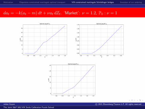
Motivation Dispersion-constrained martingale optimal transport VIX-constrained martingale Schrodinger bridges Inversion of cvx ordering
dat = −k(at −m) dt+ νat dZt. ‘Market’: ν = 1.2, P0 : ν = 1
0.6 0.8 1.0 1.2 1.4 1.6 1.8S
0
5
10
15
20
25
30
u 1(S
)
Optimal payoff u1
0.0 0.1 0.2 0.3 0.4 0.5 0.6V
0.00
0.25
0.50
0.75
1.00
1.25
1.50
1.75
u V(V
)
Optimal payoff uV
0.6 0.8 1.0 1.2 1.4 1.6 1.8S
0
5
10
15
20
25
u 2(S
)
Optimal payoff u2
Julien Guyon c© 2021 Bloomberg Finance L.P. All rights reserved.
The Joint S&P 500/VIX Smile Calibration Puzzle Solved

Motivation Dispersion-constrained martingale optimal transport VIX-constrained martingale Schrodinger bridges Inversion of cvx ordering
dat = −k(at −m) dt+ νat dZt. ‘Market’: ν = 0.9, ρ = −0.5, P0 : ν = 1,ρ = −0.3
0.7 0.8 0.9 1.0 1.1Strikes
18
20
22
24
26
28
30
Impl
ied
vola
tiliti
es in
per
cent
"SPX" implied volatilities, T1 = 0.17"Market" ( -SABR, = 0.9, = 0.5)Calibrated model ( -SABR, = 1.0, = 0.3, modified SV drift)Reference model ( -SABR, = 1.0, = 0.3)
16 18 20 22 24 26 28 30Strikes
74
76
78
80
82
84
86
Impl
ied
vola
tiliti
es in
per
cent
"VIX" implied volatilities, T1 = 0.17
"Market" ( -SABR, = 0.9)Calibrated model ( -SABR, = 1.0, = 0.3, modified SV drift)Reference model ( -SABR, = 1.0, = 0.3)"Market" VIX futureVIX future in calibrated modelVIX future in reference model
0.7 0.8 0.9 1.0 1.1Strikes
18
20
22
24
26
28
30
Impl
ied
vola
tiliti
es in
per
cent
"SPX" implied volatilities, T2 = 0.25"Market" ( -SABR, = 0.9, = 0.5)Calibrated model ( -SABR, = 1.0, = 0.3, modified SV drift)Reference model ( -SABR, = 1.0, = 0.3)
Julien Guyon c© 2021 Bloomberg Finance L.P. All rights reserved.
The Joint S&P 500/VIX Smile Calibration Puzzle Solved

Motivation Dispersion-constrained martingale optimal transport VIX-constrained martingale Schrodinger bridges Inversion of cvx ordering
Other approaches
Guo-Loeper-Ob loj-Wang (2020): joint calibration via semimartingaleoptimal transport
More general cost function: volatilities and correlations are allowed to bemodified from reference modelModel (St, Yt) instead of (St, at) where Y is the price at t of the integratedvariance over [t, T2]Terminal constraint on the semimartingale Y : YT2
= 0
Cont-Kokholm (2013): Bergomi-like model with simultaneous jumps onSPX and VIX.
Best fitAn approximation of the VIX in the model is used
Gatheral-Jusselin-Rosenbaum (2020): quadratic rough Heston volatilitymodel.
Best fitVIX smile well calibrated, not enough ATM SPX skew
Fouque-Saporito (2018): Heston Stochastic Vol-of-Vol Model
Pacati-Pompa-Reno (2018): displacement of multi-factor affine modelswith jumps (Heston++)
Papanicolaou-Sircar (2014), Goutte-Amine-Pham (2017):regime-switching Heston model (with or without jumps)
Julien Guyon c© 2021 Bloomberg Finance L.P. All rights reserved.
The Joint S&P 500/VIX Smile Calibration Puzzle Solved

Motivation Dispersion-constrained martingale optimal transport VIX-constrained martingale Schrodinger bridges Inversion of cvx ordering
Inversion of convex orderingin the VIX market
Julien Guyon c© 2021 Bloomberg Finance L.P. All rights reserved.
The Joint S&P 500/VIX Smile Calibration Puzzle Solved

Motivation Dispersion-constrained martingale optimal transport VIX-constrained martingale Schrodinger bridges Inversion of cvx ordering
Quantitative Finance (September 2020)
Quantitative Finance, 2020https://doi.org/10.1080/14697688.2020.1753885
Inversion of convex ordering in the VIX marketJULIEN GUYON*
Quantitative Research, Bloomberg L.P., 731 Lexington Ave, New York, NY 10022, USA
(Received 14 December 2019; accepted 3 April 2020 )
We investigate conditions for the existence of a continuous model on the S&P 500 index (SPX) thatjointly calibrates to a full surface of SPX implied volatilities and to the VIX smiles. We present anovel approach based on the SPX smile calibration condition E[σ 2
t |St] = σ 2lv(t, St). In the limiting
case of instantaneous VIX, a novel application of martingale transport to finance shows that suchmodel exists if and only if, for each time t, the local variance σ 2
lv(t, St) is smaller than the instanta-neous variance σ 2
t in convex order. The real case of a 30-day VIX is more involved, as averagingover 30 days and projecting onto a filtration can undo convex ordering.
We show that in usual market conditions, and for reasonable smile extrapolations, the distributionof VIX2
T in the market local volatility model is larger than the market-implied distribution of VIX2T
in convex order for short maturities T, and that the two distributions are not rankable in convex orderfor intermediate maturities. In particular, a necessary condition for continuous models to jointly cal-ibrate to the SPX and VIX markets is the inversion of convex ordering property: the fact that, eventhough associated local variances are smaller than instantaneous variances in convex order, the VIXsquared is larger in convex order in the associated local volatility model than in the original modelfor short maturities. We argue and numerically demonstrate that, when the (typically negative) spot–vol correlation is large enough in absolute value, (a) traditional stochastic volatility models withlarge mean reversion, and (b) rough volatility models with small Hurst exponent, satisfy the inver-sion of convex ordering property, and more generally can reproduce the market term-structure ofconvex ordering of the local and stochastic squared VIX.
Keywords: VIX; Convex order; Inversion of convex ordering; Martingale transport; Local volatility;Stochastic volatility; Mean reversion; Rough volatility; Smile calibration
1. Introduction
Volatility indices, such as the VIX index (CBOE 2017), do notonly serve as market-implied indicators of volatility. Futuresand options on these indices are also widely used as risk-management tools to hedge the volatility exposure of optionsportfolios. The existence of a liquid market for these futuresand options has led to the need for models that jointly cali-brate to the prices of options on the underlying asset and theprices of volatility derivatives. Without such models, finan-cial institutions could possibly arbitrage each other, and evendesks within the same institution could do so, e.g. the VIXdesk could arbitrage the SPX desk.
In particular, since VIX options started trading on theCBOE in 2006, many researchers and practitioners haveattempted to build a model for the SPX that is consistentwith market data on both SPX options and VIX futures andoptions. The first attempt, by Gatheral (2008, 2013), used adiffusive (double mean reverting) model. Interestingly, thenumerical results show that, in usual market conditions, this
*Email: [email protected]
model, though it is very flexible, cannot fit both the negativeat-the-money (ATM) SPX skew (not large enough in absolutevalue) and the ATM VIX volatility (too large) for short matu-rities (up to 5 months). One should decrease the volatility ofvolatility (‘vol-of-vol’) to decrease the latter, but this wouldalso decrease the former, which is already too small.
Guyon’s experiments (Guyon 2018a, 2018b) using veryflexible models such as the skewed two-factor Bergomi model(Bergomi 2008), the skewed rough Bergomi model, indepen-dently introduced by Guyon (2018a) and De Marco (2018),and their stochastic local volatility versions, are also suggest-ing that joint calibration seems out of the reach of classicalcontinuous-time models with continuous SPX paths (‘contin-uous models’ for short): either the SPX smile is well fitted,but then the model ATM VIX implied volatility is too large;or the VIX smile is well calibrated, but then the modelATM SPX skew is too small in absolute value. Song andXiu (2012) argued that ‘the state-of-the-art stochastic volatil-ity models in the literature cannot capture the S&P 500 andVIX option prices simultaneously’. Jacquier et al. (2018)investigated the rough Bergomi model and reached a similarconclusion:
© 2020 Informa UK Limited, trading as Taylor & Francis Group
Julien Guyon c© 2021 Bloomberg Finance L.P. All rights reserved.
The Joint S&P 500/VIX Smile Calibration Puzzle Solved

Motivation Dispersion-constrained martingale optimal transport VIX-constrained martingale Schrodinger bridges Inversion of cvx ordering
Continuous model on SPX calibrated to SPX options
dStSt
= σt dWt, S0 = x. (4.1)
Corresponding local volatility function σloc: σ2loc(t, St) := E[σ2
t |St].Corresponding local volatility model:
dSloct
Sloct
= σloc(t, Sloct ) dWt, Sloc
0 = x.
From Gyongy (1986): ∀t ≥ 0, Sloct
(d)= St.
Using Dupire (1994), we conclude that Model (4.1) is calibrated to the fullSPX smile if and only if σloc = σlv (market local volatility computed usingDupire’s formula).
Market local volatility model:
dSlvt
Slvt
= σlv(t, Slvt ) dWt, Slv
0 = x.
Julien Guyon c© 2021 Bloomberg Finance L.P. All rights reserved.
The Joint S&P 500/VIX Smile Calibration Puzzle Solved

Motivation Dispersion-constrained martingale optimal transport VIX-constrained martingale Schrodinger bridges Inversion of cvx ordering
VIX
By definition, the (idealized) VIX at time T ≥ 0 is the implied volatility ofa 30 day log-contract on the SPX index starting at T . For continuousmodels (4.1), this translates into
VIX2T = E
[1
τ
∫ T+τ
T
σ2t dt
∣∣∣∣FT ] =1
τ
∫ T+τ
T
E[σ2t
∣∣FT ] dt.Since E[σ2
loc(t, Sloct )|FT ] = E[σ2
loc(t, Sloct )|Sloc
T ], VIXloc,T satisfies
VIX2loc,T =
1
τ
∫ T+τ
T
E[σ2loc(t, Sloc
t )|SlocT ] dt = E
[1
τ
∫ T+τ
T
σ2loc(t, Sloc
t ) dt
∣∣∣∣SlocT
].
Similarly,
VIX2lv,T =
1
τ
∫ T+τ
T
E[σ2lv(t, Slv
t )|SlvT ] dt = E
[1
τ
∫ T+τ
T
σ2lv(t, Slv
t ) dt
∣∣∣∣SlvT
].
Julien Guyon c© 2021 Bloomberg Finance L.P. All rights reserved.
The Joint S&P 500/VIX Smile Calibration Puzzle Solved

Motivation Dispersion-constrained martingale optimal transport VIX-constrained martingale Schrodinger bridges Inversion of cvx ordering
Reminder on convex order
(The distributions of) two random variables X and Y are said to be inconvex order if and only if, for any convex function f , E[f(X)] ≤ E[f(Y )].
Denoted by X ≤c Y .
Both distributions have same mean, but distribution of Y is more “spread”than that of X.
In financial terms: X and Y have the same forward value, but calls(puts) on Y are more expensive than calls (puts) on X (dimension 1).
Julien Guyon c© 2021 Bloomberg Finance L.P. All rights reserved.
The Joint S&P 500/VIX Smile Calibration Puzzle Solved

Motivation Dispersion-constrained martingale optimal transport VIX-constrained martingale Schrodinger bridges Inversion of cvx ordering
The case of instantaneous VIX: τ → 0
Assume SV model is calibrated to the SPX smile: E[σ2t |St] = σ2
lv(t, St).
As observed by Dupire (2005), by conditional Jensen, σ2lv(t, St) ≤c σ2
t , i.e.,
mkt local vart ≤c instVIX2t .
Conversely, if mkt local vart ≤c instVIX2t , there exists a jointly calibrating
SPX/instVIX model (G., 2017).
=⇒ Convex order condition is necessary and sufficient for instVIX.
Proof uses a new type of application of martingale transport tofinance: martingality constraint applies to (mkt local vart, instVIX2
t ) at asingle date, instead of (S1, S2).
Julien Guyon c© 2021 Bloomberg Finance L.P. All rights reserved.
The Joint S&P 500/VIX Smile Calibration Puzzle Solved

Motivation Dispersion-constrained martingale optimal transport VIX-constrained martingale Schrodinger bridges Inversion of cvx ordering
The real VIX: τ = 30 days
In reality, squared VIX are not instantaneous variances but the fair strikesof 30-day realized variances.
Let us look at market data (August 1, 2018). We compare the marketdistributions of
VIX2lv,T := E
[1
τ
∫ T+τ
T
σ2lv(t, Slv
t ) dt
∣∣∣∣SlvT
]and
VIX2mkt,T
(←→ E
[1
τ
∫ T+τ
T
σ2t dt
∣∣∣∣FT ])
Julien Guyon c© 2021 Bloomberg Finance L.P. All rights reserved.
The Joint S&P 500/VIX Smile Calibration Puzzle Solved

Motivation Dispersion-constrained martingale optimal transport VIX-constrained martingale Schrodinger bridges Inversion of cvx ordering
T = 21 days
Julien Guyon c© 2021 Bloomberg Finance L.P. All rights reserved.
The Joint S&P 500/VIX Smile Calibration Puzzle Solved

Motivation Dispersion-constrained martingale optimal transport VIX-constrained martingale Schrodinger bridges Inversion of cvx ordering
T = 21 days
Julien Guyon c© 2021 Bloomberg Finance L.P. All rights reserved.
The Joint S&P 500/VIX Smile Calibration Puzzle Solved

Motivation Dispersion-constrained martingale optimal transport VIX-constrained martingale Schrodinger bridges Inversion of cvx ordering
T = 21 days
Julien Guyon c© 2021 Bloomberg Finance L.P. All rights reserved.
The Joint S&P 500/VIX Smile Calibration Puzzle Solved

Motivation Dispersion-constrained martingale optimal transport VIX-constrained martingale Schrodinger bridges Inversion of cvx ordering
VIX2lv,T (Slv
T )
Julien Guyon c© 2021 Bloomberg Finance L.P. All rights reserved.
The Joint S&P 500/VIX Smile Calibration Puzzle Solved

Motivation Dispersion-constrained martingale optimal transport VIX-constrained martingale Schrodinger bridges Inversion of cvx ordering
T = 77 days
Julien Guyon c© 2021 Bloomberg Finance L.P. All rights reserved.
The Joint S&P 500/VIX Smile Calibration Puzzle Solved

Motivation Dispersion-constrained martingale optimal transport VIX-constrained martingale Schrodinger bridges Inversion of cvx ordering
T = 77 days
Julien Guyon c© 2021 Bloomberg Finance L.P. All rights reserved.
The Joint S&P 500/VIX Smile Calibration Puzzle Solved
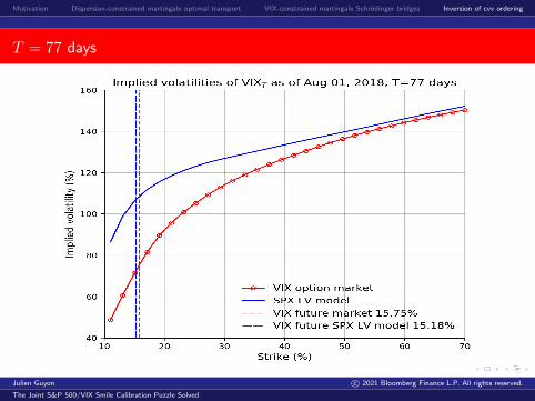
Motivation Dispersion-constrained martingale optimal transport VIX-constrained martingale Schrodinger bridges Inversion of cvx ordering
T = 77 days
Julien Guyon c© 2021 Bloomberg Finance L.P. All rights reserved.
The Joint S&P 500/VIX Smile Calibration Puzzle Solved

Motivation Dispersion-constrained martingale optimal transport VIX-constrained martingale Schrodinger bridges Inversion of cvx ordering
Inversion of convex ordering
Inversion of convex ordering: the fact that, for small T ,VIX2
loc,T ≥c VIX2T despite the fact that for all t, σ2
loc(t, St) ≤c σ2t .
A necessary condition for continuous models to jointly calibrate to theSPX and VIX markets.In the paper, we numerically show that when the spot-vol correlation islarge enough in absolute value,(a) traditional SV models with large mean reversion, and(b) rough volatility models with small Hurst exponent
satisfy the inversion of convex ordering property, and more generally canreproduce the market term-structure of convex ordering of the local andstochastic squared VIX.
Not a sufficient condition though.
Actually we have proved that inversion of convex ordering can beproduced by a continuous SV model.
In such models, for small T , VIX2loc,T >c VIX2
T so (x 7→√x concave)
E[VIXT ] > E [VIXloc,T ] :
Local volatility does NOT maximize the price of VIX futures.
Julien Guyon c© 2021 Bloomberg Finance L.P. All rights reserved.
The Joint S&P 500/VIX Smile Calibration Puzzle Solved
Motivation Dispersion-constrained martingale optimal transport VIX-constrained martingale Schrodinger bridges Inversion of cvx ordering
SIAM J. Financial Math. 11(1):SC1–SC13, 2020 (with B. Acciaio)
SIAM J. FINANCIAL MATH. c\bigcirc 2020 Society for Industrial and Applied MathematicsVol. 11, No. 1, pp. SC1--SC13
Short Communication: Inversion of Convex Ordering: Local Volatility Does NotMaximize the Price of VIX Futures\ast
Beatrice Acciaio\dagger and Julien Guyon\ddagger
Abstract. It has often been stated that, within the class of continuous stochastic volatility models calibratedto vanillas, the price of a VIX future is maximized by the Dupire local volatility model. In thisarticle we prove that this statement is incorrect: we build a continuous stochastic volatility modelin which a VIX future is strictly more expensive than in its associated local volatility model. Moregenerally, in our model, strictly convex payoffs on a squared VIX are strictly cheaper than in theassociated local volatility model. This corresponds to an inversion of convex ordering between localand stochastic variances, when moving from instantaneous variances to squared VIX, as convexpayoffs on instantaneous variances are always cheaper in the local volatility model. We thus provethat this inversion of convex ordering, which is observed in the S\&P 500 market for short VIXmaturities, can be produced by a continuous stochastic volatility model. We also prove that themodel can be extended so that, as suggested by market data, the convex ordering is preserved forlong maturities.
Key words. VIX, VIX futures, stochastic volatility, local volatility, convex order, inversion of convex ordering
AMS subject classifications. 91G20, 91G80, 60H30
DOI. 10.1137/19M129303X
1. Introduction. For simplicity, let us assume zero interest rates, repos, and dividends.Let \scrF t denote the market information available up to time t. We consider continuous stochasticvolatility models on the S\&P 500 index (SPX) of the form
dStSt
= \sigma t dWt, S0 = s0,(1.1)
where W = (Wt)t\geq 0 denotes a standard one-dimensional (\scrF t)-Brownian motion, \sigma = (\sigma t)t\geq 0
is an (\scrF t)-adapted process such that\int t0 \sigma
2s ds < \infty a.s. for all t \geq 0, and s0 > 0 is the initial
SPX price. By ``continuous model"" we mean that the SPX has no jump, while the volatilityprocess \sigma may be discontinuous. The local volatility function associated to model (1.1) is thefunction \sigma \mathrm{l}\mathrm{o}\mathrm{c} defined by
\sigma 2\mathrm{l}\mathrm{o}\mathrm{c}(t, x) := \BbbE [\sigma 2t | St = x].(1.2)
The associated local volatility model is defined by
dS\mathrm{l}\mathrm{o}\mathrm{c}t
S\mathrm{l}\mathrm{o}\mathrm{c}t
= \sigma \mathrm{l}\mathrm{o}\mathrm{c}(t, S\mathrm{l}\mathrm{o}\mathrm{c}t ) dWt, S\mathrm{l}\mathrm{o}\mathrm{c}
0 = s0.
\ast Received by the editors October 14, 2019; accepted for publication (in revised form) December 18, 2019;published electronically February 20, 2020.
https://doi.org/10.1137/19M129303X\dagger Department of Statistics, London School of Economics and Political Science, London WC2A 2AE, UK
([email protected]).\ddagger Quantitative Research, Bloomberg L.P., New York, NY 10022 ([email protected]).
SC1
Julien Guyon c© 2021 Bloomberg Finance L.P. All rights reserved.
The Joint S&P 500/VIX Smile Calibration Puzzle Solved

Motivation Dispersion-constrained martingale optimal transport VIX-constrained martingale Schrodinger bridges Inversion of cvx ordering
Thanks!
Julien Guyon c© 2021 Bloomberg Finance L.P. All rights reserved.
The Joint S&P 500/VIX Smile Calibration Puzzle Solved

Motivation Dispersion-constrained martingale optimal transport VIX-constrained martingale Schrodinger bridges Inversion of cvx ordering
A few selected references
Acciaio, B., Guyon, J.: Inversion of Convex Ordering: Local Volatility Does Not
Maximize the Price of VIX Futures, SIAM J. Financial Math. 11(1):SC1–SC13,2020.
Beiglbock, M., Henry-Labordere, P., Penkner, F.: Model-independent bounds for
option prices: A mass-transport approach, Finance Stoch., 17(3):477–501, 2013.
Blaschke, W, Pick, G.: Distanzschatzungen im Funktionenraum II, Math. Ann.77:277–302, 1916.
Carr, P., Madan, D.: Joint modeling of VIX and SPX options at a single andcommon maturity with risk management applications, IIE Transactions46(11):1125–1131, 2014.
Cont, R., Kokholm, T.: A consistent pricing model for index options and
volatility derivatives, Math. Finance 23(2):248–274, 2013.
Cuturi, M.: Sinkhorn distances: Lightspeed computation of optimal transport,Advances in neural information processing systems, 2292–2300, 2013.
De March, A.: Entropic approximation for multi-dimensional martingale optimaltransport, preprint, arXiv, 2018.
Julien Guyon c© 2021 Bloomberg Finance L.P. All rights reserved.
The Joint S&P 500/VIX Smile Calibration Puzzle Solved

Motivation Dispersion-constrained martingale optimal transport VIX-constrained martingale Schrodinger bridges Inversion of cvx ordering
A few selected references
De March, A., Henry-Labordere, P.: Building arbitrage-free implied volatility:Sinkhorn’s algorithm and variants , preprint, SSRN, 2019.
De Marco, S., Henry-Labordere, P.: Linking vanillas and VIX options: Aconstrained martingale optimal transport problem, SIAM J. Financial Math.6:1171–1194, 2015.
Dupire, B.: Pricing with a smile, Risk, January, 1994.
Fouque, J.-P., Saporito, Y.: Heston Stochastic Vol-of-Vol Model for JointCalibration of VIX and S&P 500 Options, Quantitative Finance18(6):1003–1016, 2018.
Gatheral, J.: Consistent modeling of SPX and VIX options, presentation atBachelier Congress, 2008.
Gatheral, J., Jusselin, P., Rosenbaum, M.: The quadratic rough Heston modeland the joint calibration problem, Risk, May 2020.
Goutte, S, Amine, I., and Pham, H.: Regime-switching stochastic volatilitymodel: estimation and calibration to VIX options, Applied Math. Finance24(1):38–75, 2017.
Julien Guyon c© 2021 Bloomberg Finance L.P. All rights reserved.
The Joint S&P 500/VIX Smile Calibration Puzzle Solved
Motivation Dispersion-constrained martingale optimal transport VIX-constrained martingale Schrodinger bridges Inversion of cvx ordering
A few selected references
Guo, I., Loeper, G., Ob loj, J., Wang, S.: Joint Modelling and Calibration of SPXand VIX by Optimal Transport, preprint, 2020.
Guyon, J., Menegaux, R., Nutz, M.: Bounds for VIX futures given S&P 500
smiles, Finan. & Stoch. 21(3):593–630, 2017.
Guyon, J.: On the joint calibration of SPX and VIX options, Conference in honorof Jim Gatheral’s 60th birthday, NYU Courant, 2017. And Finance andStochastics seminar, Imperial College London, 2018.
Guyon, J.: The Joint S&P 500/VIX Smile Calibration Puzzle Solved, Risk, April2020.
Guyon, J.: Inversion of convex ordering in the VIX market, Quantitative Finance
20(10):1597–1623, 2020.
Henry-Labordere, P.: Automated Option Pricing: Numerical Methods, Intern.
Journ. of Theor. and Appl. Finance 16(8), 2013.
Henry-Labordere, P.: Model-free Hedging: A Martingale Optimal Transport
Viewpoint, Chapman & Hall/CRC Financial Mathematics Series, 2017.
Julien Guyon c© 2021 Bloomberg Finance L.P. All rights reserved.
The Joint S&P 500/VIX Smile Calibration Puzzle Solved

Motivation Dispersion-constrained martingale optimal transport VIX-constrained martingale Schrodinger bridges Inversion of cvx ordering
A few selected references
Jacquier, A., Martini, C., Muguruza, A.: On the VIX futures in the rough
Bergomi model, Quantitative Finance 18(1):45–61, 2018.
Johansen, S.: The extremal convex functions. Math. Scand., 34, 61–68 (1974)
Kokholm, T., Stisen, M.: Joint pricing of VIX and SPX options with stochastic
volatility and jump models, The Journal of Risk Finance 16(1):27–48, 2015.
Pacati, C., Pompa, P., Reno, R.: Smiling Twice: The Heston++ Model, Journal
of Banking & Finance, Elsevier, 96(C):185–206, 2018.
Papanicolaou, A., Sircar, R.: A regime-switching Heston model for VIX and S&P
500 implied volatilities, Quantitative Finance 14(10):1811–1827, 2014.
Sinkhorn, R.: Diagonal equivalence to matrices with prescribed row and column
sums, The American Mathematical Monthly, 74(4):402–405, 1967.
Strassen, V.: The existence of probability measures with given marginals, Ann.Math. Statist., 36:423–439, 1965.
Julien Guyon c© 2021 Bloomberg Finance L.P. All rights reserved.
The Joint S&P 500/VIX Smile Calibration Puzzle Solved

Motivation Dispersion-constrained martingale optimal transport VIX-constrained martingale Schrodinger bridges Inversion of cvx ordering
Risk, April 2020
Julien Guyon c© 2021 Bloomberg Finance L.P. All rights reserved.
The Joint S&P 500/VIX Smile Calibration Puzzle Solved

Motivation Dispersion-constrained martingale optimal transport VIX-constrained martingale Schrodinger bridges Inversion of cvx ordering
Equations for u∗ = (u∗1, u∗V , u
∗2,∆
∗S ,∆
∗L)
∂Ψµ∂u1(s1)
=0 : ∀s1 > 0, u1(s1) = Φ1(s1;uV , u2,∆S ,∆L)
∂Ψµ∂uV (v)
=0 : ∀v ≥ 0, uV (v) = ΦV (v;u1, u2,∆S ,∆L)
∂Ψµ∂u2(s2)
=0 : ∀s2 > 0, u2(s2) = Φ2(s2;u1, uV ,∆S ,∆L)
∂Ψµ∂∆S(s1,v)
=0 : ∀s1 > 0, ∀v ≥ 0, 0 = Φ∆S (s1, v; ∆S(s1, v),∆L(s1, v))
∂Ψµ∂∆L(s1,v)
=0 : ∀s1 > 0, ∀v ≥ 0, 0 = Φ∆L(s1, v; ∆S(s1, v),∆L(s1, v))
Φ1(s1;uV ,∆S,∆L) := lnµ1(s1) − ln
∫ µ(s1, dv, ds2)euV (v)+u2(s2)+∆
(S)S
(s1,v,s2)+∆(L)L
(s1,v,s2)
ΦV (v;u1,∆S,∆L) := lnµV (v) − ln
∫ µ(ds1, v, ds2)eu1(s1)+u2(s2)+∆
(S)S
(s1,v,s2)+∆(L)L
(s1,v,s2)
Φ2(s2;u1, uV ,∆S,∆L) := lnµ2(s2) − ln
∫ µ(ds1, dv, s2)eu1(s1)+uV (v)+∆
(S)S
(s1,v,s2)+∆(L)L
(s1,v,s2)
Φ∆S(s1, v;u2, δS, δL) :=
∫µ(s1, v, ds2)(s2 − s1)e
u2(s2)+δS(s2−s1)+δL
(L
(s2s1
)−v2
)
Φ∆L(s1, v;u2, δS, δL) :=
∫µ(s1, v, ds2)
(L
(s2
s1
)− v2
)eu2(s2)+δS(s2−s1)+δL
(L
(s2s1
)−v2
).
Julien Guyon c© 2021 Bloomberg Finance L.P. All rights reserved.
The Joint S&P 500/VIX Smile Calibration Puzzle Solved

Motivation Dispersion-constrained martingale optimal transport VIX-constrained martingale Schrodinger bridges Inversion of cvx ordering
Implementation details
Practically, we consider market strikes K := (K1,KV ,K2) and market prices(C1
K , CVK , C
2K) of vanilla options on S1, V , and S2, and we build the model
µ∗K(ds1, dv, ds2) = µ(ds1, dv, ds2)ec∗+∆0∗
S s1+∆0∗V v+
∑K∈K1
a1∗K (s1−K)+
e∑K∈KV
aV ∗K (v−K)++∑K∈K2
a2∗K (s2−K)++∆
∗(S)S
(s1,v,s2)+∆∗(L)L
(s1,v,s2)
where θ∗ := (c∗,∆0∗S ,∆
0∗V , a
1∗, aV ∗, a2∗,∆∗S ,∆∗L) maximizes
Ψµ,K(θ) := c+ ∆0SS0 + ∆0
V FV +∑K∈K1
a1KC
1K +
∑K∈KV
aVKCVK +
∑K∈K2
a2KC
2K
−Eµ[ec+∆0
SS1+∆0V V+
∑K1
a1K(S1−K)++
∑KV
aVK(V−K)++∑K2
a2K(S2−K)++∆
(S)S
(...)+∆(L)L
(...)
]over the set Θ of portfolios θ := (c,∆0
S ,∆0V , a
1, aV , a2,∆S ,∆L) such thatc,∆0
S ,∆0V ∈ R, a1 ∈ RK1 , aV ∈ RKV , a2 ∈ RK2 , and
∆S ,∆L : R>0 × R≥0 → R are measurable functions of (s1, v).
Julien Guyon c© 2021 Bloomberg Finance L.P. All rights reserved.
The Joint S&P 500/VIX Smile Calibration Puzzle Solved

Motivation Dispersion-constrained martingale optimal transport VIX-constrained martingale Schrodinger bridges Inversion of cvx ordering
Implementation details
This corresponds to solving the entropy minimization problem
Pµ,K := infµ∈P(K)
H(µ, µ) = supθ∈Θ
Ψµ,K(θ) =: Dµ,K
where P(K) denotes the set of probability measures µ onR>0 × R≥0 × R>0 such that
Eµ[S1] = S0, Eµ[V ] = FV , ∀K ∈ K1, Eµ [(S1 −K)+] = C1K ,
∀K ∈ KV , Eµ [(V −K)+] = CVK , ∀K ∈ K2, Eµ [(S2 −K)+] = C2K ,
Eµ [S2|S1, V ] = S1, Eµ[L
(S2
S1
)∣∣∣∣S1, V
]= V 2.
One can directly check that model µ∗K is an arbitrage-free model thatjointly calibrates the prices of SPX futures, options, VIX future, and VIXoptions. Indeed, if Ψµ,K reaches its maximum at θ∗, then θ∗ is solution to∂Ψµ,K∂θi
(θ) = 0:
Julien Guyon c© 2021 Bloomberg Finance L.P. All rights reserved.
The Joint S&P 500/VIX Smile Calibration Puzzle Solved

Motivation Dispersion-constrained martingale optimal transport VIX-constrained martingale Schrodinger bridges Inversion of cvx ordering
Implementation details
Ψµ,K(θ) := c+ ∆0SS0 + ∆0
V FV +∑K∈K1
a1KC
1K +
∑K∈KV
aVKCVK +
∑K∈K2
a2KC
2K
−Eµ[ec+∆0
SS1+∆0V V+
∑K1
a1K(S1−K)++
∑KV
aVK(V−K)++∑K2
a2K(S2−K)++∆
(S)S
(...)+∆(L)L
(...)
]∂Ψµ,K∂c
= 0 : Eµ[dµ∗Kdµ
]= 1
∂Ψµ,K∂∆0
S
= 0 : Eµ[S1dµ∗Kdµ
]= S0
∂Ψµ,K∂∆0
V
= 0 : Eµ[Vdµ∗Kdµ
]= FV
∂Ψµ,K∂a1
K
= 0 : Eµ[(S1 −K)+
dµ∗Kdµ
]= C1
K
∂Ψµ,K∂aVK
= 0 : Eµ[(V −K)+
dµ∗Kdµ
]= CVK
∂Ψµ,K∂a2
K
= 0 : Eµ[(S2 −K)+
dµ∗Kdµ
]= C2
K
∂Ψµ,K∂∆S(s1, v)
= 0 : Eµ[(S2 − S1)
dµ∗Kdµ
∣∣∣∣S1 = s1, V = v
]= 0, ∀s1 ≥ 0, v > 0
∂Ψµ,K∂∆L(s1, v)
= 0 : Eµ[(L
(S2
S1
)− V 2
)dµ∗Kdµ
∣∣∣∣S1 = s1, V = v
]= 0, ∀s1 ≥ 0, v > 0
Julien Guyon c© 2021 Bloomberg Finance L.P. All rights reserved.
The Joint S&P 500/VIX Smile Calibration Puzzle Solved

Motivation Dispersion-constrained martingale optimal transport VIX-constrained martingale Schrodinger bridges Inversion of cvx ordering
SLV calibrated to SPX: VIX smile (Aug 1, 2018)
All continuous models on SPX that are calibrated to full SPX smile are ofthe form:
dStSt
=at√
E[a2t |St]
σloc(t, St) dWt.
They are stochastic local volatility (SLV) models
dStSt
= at`(t, St) dWt
with stochastic volatility (SV) (at) and leverage function
`(t, St) =σloc(t, St)√E[a2
t |St].
In those models (τ := 30 days)
VIX2T =
1
τ
∫ T+τ
T
E[
a2t
E[a2t |St]
σ2loc(t, St)
∣∣∣∣FT ] dt.Optimize SV parameters to fit VIX options.
Julien Guyon c© 2021 Bloomberg Finance L.P. All rights reserved.
The Joint S&P 500/VIX Smile Calibration Puzzle Solved

Motivation Dispersion-constrained martingale optimal transport VIX-constrained martingale Schrodinger bridges Inversion of cvx ordering
SLV calibrated to SPX: VIX smile, T = 21 days (Aug 1, 2018)
SLV model, SV = skewed 2-factor Bergomi modelSV params optimized to fit VIX smile
Julien Guyon c© 2021 Bloomberg Finance L.P. All rights reserved.
The Joint S&P 500/VIX Smile Calibration Puzzle Solved