the journal of undergraduate research in natural sciences

1

The Journal of Undergraduate Research in Natural Sciences and Mathematics

Volume 15 Spring 2013

California State University, Fullerton

1







DIM

ENSIO

NS


2

MARKS OF A CSUF GRADUATE FROM THE COLLEGE OF NATURAL SCIENCES AND MATHEMATICS

Graduates from the College of Natural Sciences and Mathematics:

Understand the basic concepts and principles of science and mathematics.

Are experienced in working collectively and collaborating to solve problems.

Communicate both orally and in writing with clarity, precision and confidence.

Are adept at using computers to do word processing, prepare spreadsheets and graphs, and use presentation software.

Posses skills in information retrieval using library resources and the Internet.

Have extensive laboratory/workshop/field experience where they utilize the scientific method to ask questions, formulate hypothesis, design experiments, conduct experiments, and analyze data.

Appreciate diverse cultures as a result of working side by side with many people in collaborative efforts in the classroom, laboratory and on research projects.

In many instances have had the opportunity to work individually with faculty in conducting research and independent projects. In addition to attribtes of all NSM students, these students generate original data and contribute to the reseach knowledge base.

Have had the opportunity to work with very modern, sophisticated equipment including advanced computer hardware and software.

3

DIMENSIONS ABOUT THE COVER

Dimensions: The Journal of Undergraduate Research in Natural Sciences and Mathematics is an official publication of California State University, Fullerton. Dimensions is published annually by CSUF, 800 N. St. College Blvd., Fullerton, CA 92834. Copyright ©2012 CSUF. Except as otherwise provided, Dimensions: The Journal of Undergraduate Research in Natural Sciences and Mathematics grants permission for material in this publication to be copied for use by non-profit educational institutions for scholarly or instructional purposes only, provided that 1) copies are distributed at or below cost, 2) the author and Dimensions are identified, and 3) proper notice of copyright appears on each copy. If the author retains the copyright, permission to copy must be attained directly from the author.

In our everyday lives we are surrounded and submersed in the unknown, from the largest mountains to the miniscule atoms. We are constantly on the search to satisfy our curiosity to gather knowledge and understanding of all that surrounds us.

This journal is a testament to our yearning to fulfill our curiosity through scientific research.

Through exploration, we may better understand our surroundings. The wilderness signifies the unknown, and all that remains to be explored, with mountainous challenges to be conquered along the way.

4

ACKNOWLEDGEMENTS

EDITOR-IN-CHIEFChris Baker

EDITORSNeha Ansari, Chemistry/BiochemistryNghia Tran, ChemistryErik Cadaret, GeologyKelly Hartmann, MathematicsRobert Wright, Physics

ADVISORAmy Mattern, Interim Assistant Dean for Student Affairs

GRAPHIC DESIGNTiffany Le, Cover Designer/Layout Editor

COLLEGE OF NATURAL SCIENCES & MATHEMATICSDr. Robert A. Koch, Acting DeanDr. Mark Filowitz, Associate DeanDr. Kathryn Dickson, Acting Chair Department of Biological ScienceDr. Christopher Meyer, Chair Department of ChemistryDr. David Bowman, Chair Department of Geological SciencesDr. Stephen Goode, Chair Department of MathematicsDr. James M. Feagin, Chair Department of Physics

COLLEGE OF THE ARTSDr. Joseph H. Arnold, DeanAndi Sims, Assistant Dean for Student AffairsArnold Holland, Graphic Design ProfessorJohn Drew, Graphic Design Professor

SPECIAL THANKS TOPresident Mildred García and Dean Robert A. Koch for their support and dedication to Dimensions.

5

ARTICLES

021 043

009 030

055

008 028

027 051

018 031

BIOLOGY CHEMISTRY AND BIOCHEMISTRY

Nest Predation Risk in Suburban versus Grassland Edges Associated with Adjacent Coastal Sage Scrub InteriorsEric Kessler, Ignacio Vera, Tuong-Vy Nguyen, Nicole Tronske, Cristy Rice, William Hoese

Aqueous Phase Oxidation of Succinic Acid by Hydroxyl Radicals. Part I. Hygroscopic Behavior of the Reaction Products.Aaron Ninokawa, Shaun Cook, Trent Northen, Paula K. Hudson

Patterns of Activity and Diversity of Bats at the Urban-Wildland Interface in Southern California Lauren Dorough

Mechanistic Studies on the Intramolecular Reactions of Iminoxyl Radicals and Oxime Radical Cations with Built-in NucleophilesBrittany Grassbaugh, Wanshin Kim, Quan Tran, Peter de Lijser

Is DMT1 Involved in the Uptake of Copper by Intestinal Cells? Cole Wheadon, Maria C. Linder

The Effect of Constructed Oyster Beds on Clam Density and RichnessAndres Cisneros, Danielle C. Zacherl, Scottie Henderson

Structural Characterization of Unknown Proteins Via Computer Modeling to Determine Their Biochemical PathwaysBrian Giolli

Foraging Behavior Of Kangaroo Rats At Seed Trays Revealed By Giving-Up Densities And Remote CamerasDylan Tennant

Electrochemical Surface Modification of Palladium by Antimony, Lead, and Tin, for the Electro-Oxidation of Small Organic (Alcohol) Molecules in Alkaline MediaAmissi Sadiki, Paul Vo, Grant Ognibene, Jennifer Tran, Phil Motevosian, John L. Haan

Father-Child Relationship and Children’s OutcomesQuinn Howard, Auriana Arabpour

Aqueous Phase Oxidation of Succinic Acid by Hydroxyl Radicals. Part II. Product Composition and MechanismsJulie L. Hofstra, H. J. Peter de Lijser, Paula K. Hudson

6

073

064

063

GEOLOGY

Metasomatism of the Bird Spring Formation near Slaughterhouse Springs, CaliforniaTaylor Kennedy

A Detrital Zircon Study of the Oldest Sediments in the Peninsular Ranges forearc basin, Orange County, CaliforniaNatalie Hollis

Early to Late Holocene Paleoclimate Reconstruction Using Sediment Cores from Silver Lake, Mojave Desert, CaliforniaHolly Eeg

ARTICLES

075

094

085

105

082

099

090

MATHEMATICSRobust Statistical Modeling of Neuronal Intensity Rates Jenny Chang

Comparison of Two Models For Fat/Water Separation in Magnetic Resonance Imaging (MRI)Cody Gruebele

Introducing Fundamental Algebra Concepts in Fullerton Mathematical Circle: An Approach for AMC 10 Preparation SessionRebecca Etnyre, Kelly Hartmann, Lucy H. Odom

A Statistical Approach to Validate a Cognitive Test for Multiple Sclerosis Brayan Ortiz

Inequalities Obtained from the Isoperimetric Inequality for Planar CurvesAsha Cyrs

Model Analysis in Proof SchemesKelly Hartmann

A Multivariate Statistical Inference for the Analysis of Neuronal Spiking RatesReina Galvez, Duy Ngo, Antouneo Kassab

7

115 125

119

123

PHYSICSUsing F-Test in Microarray ExperimentsEmily Ramos, Duy Ngo, Calvin Pham, Suzette Puente, Kristen Cunanan, Atousa Karimi, Gülhan Bourget

Characterizing the Optical Scatter of an Advanced LIGO Viewport Cinthia Padilla

Comparison of F and Hotelling's T2 Statistics in Microarray ExperimentsEmily Ramos, Duy Ngo, Calvin Pham, Suzette Puente, Kristen Cunanan, Atousa Karimi, Gülhan Bourget

Bijections and Roots of Polynomials in Finite FieldsNicholas Salinas

8

Clams are important to marine ecosystems as filter feeders that increase water clarity, rework sediments, and contribute to shell production - activities that can each significantly change benthic environments. We examined the effects of constructed oyster beds on density and richness of clams. On a mudflat in Newport Bay, CA we constructed replicate (n=5 per treatment) 2m X 2m oyster beds from dead oyster shell of 4 treatment types, including 2 bed thicknesses (4cm versus 12cm) and 2 consolidation types (bagged versus loose shell), plus 5 control plots. We hypothesized that constructed oyster beds, regardless of treatment type, would cause a decline in density and richness of clams relative to control plots because the shell beds would, for clams, prevent access to the mudflat surface. We sampled 25cm X 25cm X 10cm depth clam cores at 0 and 6 months and excavated 25cm X 25cm oyster bed samples at 0, 6 and 12 months. We assessed density and richness of clams per unit area by identifying live clams to species, and examined the effects of treatment, time, and their interactions. After 6 months, density of non-native Venerupis philippinarum increased significantly on all plots regardless of treatment, while densities of other species remained unchanged. However, after 12 months, clam species richness within excavated beds was highest on 12cm thick beds, regardless of consolidation type. Surprisingly, oyster beds may function to not only increase epifaunal diversity, but also clam density and richness, perhaps by offering protection from predators to the clam population.

The Effect of Constructed Oyster Beds on Clam Density and RichnessDepartment of Biology, College of Natural Sciences and Mathematics, California State University, Fullerton, CA, USA

Andres Cisneros, Danielle C. Zacherl, Scottie Henderson

Abstract

9

Habitat loss and fragmentation pose a significant threat to bat populations. Urbanization can decrease roosting sites and foraging habitat for many species in southern California. The factors that allow some species to persist in cities and suburban areas, while others decline, are unclear. We used acoustic detectors (Pettersson D240X) to record bat echolocation calls at four sites in the eastern San Gabriel Valley that differed in local site characteristics and the degree of urbanization of the surrounding landscape. Each site was sampled for ten nights between March and August 2012. Using Sonobat software to identify 6,439 calls, we detected eight bat species. Activity of the four most common species differed among sites: Tadarida brasiliensis was recorded at all sites, but was the most active species at two golf courses; Myotis yumanensis was the most common species at a large regional park; and Eptesicus fuscus and Lasiurus cinereus were the most common species at an ecological reserve. Although the reserve had the least bat activity and lowest mean species richness (based on calls), it had the highest species richness after adjusting for the number of calls. Community composition differed significantly between the sites except for the golf courses, which were not different from one another. Our results suggest that bats are abundant in areas of southern California where suitable roosting and foraging habitats are available. Understanding how bats are affected by the loss and fragmentation of natural habitats will aid in regional bat conservation efforts.

Natural environments in the United States and throughout the world have become increasingly urbanized. Natural landscapes are being converted to urban-industrialized landscapes at a rapid rate that is not projected to cease. In 1975, 74% of the United States human population lived in urban conditions. By 2009, that number had increased to 82% and the projected level of urban populations is expected to increase to 90% by 2050 (United Nations 2010). As urban populations increase, more and more natural habitats are lost or fragmented, which is a central threat to the persistence of many native species in the United States (Czech and Krausman 1997).

Abstract

Introduction

Patterns of Activity and Diversity of Bats at the Urban-Wildland Interface in Southern California

Department of Biology, College of Natural Sciences and Mathematics, California State University, Fullerton, CA, USA

Lauren DoroughAdvisor: Dr. Paul Stapp

Habitat destruction and disturbance can result in a decrease in native plant diversity, either directly or as a consequence of invasion and establishment of exotic species (Forman 1995). Typically we associate high landscape diversity with high animal species richness. The more diverse a landscape is, the more species it can usually accommodate (Savard et al. 2000). Alternatively, urbanization can generate new habitats, such as parks, golf courses, agricultural areas, and gardens, that may be suitable for some wildlife species (Hourigan et al. 2010). We have an intuitive understanding that urbanization destroys habitat for many native species, but in some cases it can result in new ones being formed, especially for species that are capable of using man-made habitats. Bat species differ in their ability to tolerate an increasingly urbanized environment (Hourigan et al. 2010, Gehrt and Chelsvig 2003, Bartonicka and Zukal 2003, Haupt et al. 2006). The factors that allow some species of bats to survive in urban cities and landscapes, while others perish, are unclear. For any bat species to survive and thrive in a given area, requirements such as roosting substrates and prey must be met (Avila-Flores and Fenton 2005). Some species can use man-made structures for roosting and others can take advantage of artificial water sources as foraging locations (Haupt et al. 2006, Rosenstock et al. 1999, Kuenzi and Morrison 2003). For other species, the loss of vegetation and natural open space results in the loss of roosts, foraging habitat, and insect prey (Avila-Flores and Fenton 2005). Ultimately, population declines of many bat species have been ascribed to anthropogenic causes (Johnson et al. 2008). The United States is home to at least 45 different species of bats, seven of which are in danger of extinction (U.S. Fish & Wildlife Service 2006). In California, little is known about the effects of urbanization on native bat species. Some 24 species of bats are found in southern California, 16 of which are considered sensitive to human disturbance (Miner and Stokes 2005). California’s human population grew by four million between 2000 and 2010 (US Census Bureau 2010). This growing population puts increasing demands on remaining natural habitats. Consequently, southern California has more endangered species than

10

most other states (Dobson et al. 1997). Studies in other parts of the U.S. have found different relationships between bat activity and diversity and increasing habitat fragmentation, isolation, and urbanization. Kurta and Teramino (1992) found a significant decrease in bat activity in urban habitats in Michigan compared to rural habitats. In contrast, Gehrt and Chelsvig (2003) reported that, although natural woodland habitats had high bat activity in Illinois, there were also high levels of bat activity at industrial and commercial sites. Several studies have demonstrated that many bat species can use urbanized habitats, while others cannot (Hourigan et al. 2010, Gehrt and Chelsvig 2003, Bartonicka and Zukal 2003, Haupt et al. 2006). These studies have provided important information about how urbanization affects bats in the eastern and midwestern United States, as well as other parts of the world. However, they may not be applicable to bats in the western United States, which is drier and has greater topographical relief compared to the wooded habitats of the east and midwest. Bats perform essential ecological services in their role as the primary predators of nocturnal insects and as key pollinators and seed dispersers for economically important plants (Kunz et al. 2011). To conserve bat species effectively it is important to understand the habitats in which bats thrive, as well as to define what levels of urbanization allow for the most diversity and activity. The objective of our research was to determine how bat activity and diversity are affected by urbanization and landscape heterogeneity in southern California. Additionally, we sought to evaluate how local habitat and landscape-level characteristics, both natural and anthropogenic, influence bat activity and diversity within different landscape types associated with water bodies. We hypothesized that bat activity and diversity would be lowest at sites with high levels of urbanization and less natural vegetation. We used acoustic monitoring to quantify bat activity and diversity at sites in the eastern San Gabriel Valley with differing landscape and local habitat characteristics.

Study Area Our study was conducted at four sites within the eastern San Gabriel Valley in southern California (Fig. 1). The eastern San Gabriel Valley encompasses an area of over 322 km2 and in 2011, had a human population size of approximately 900,000 individuals. The area is at an elevation of approximately 240 m and the native vegetation is characterized as mostly coastal sage scrub and chaparral. Average annual temperature ranges from approximately 12 – 24oC, with average annual precipitation of approximately 6 cm per year (East San Gabriel Valley, California 2011 http://www.city-data.com/city/East-San-Gabriel-Valley-California.html). The four study sites differed in the level of urbanization. The sites were: Robert J. Bernard Biological Field Station in Claremont (BFS), Frank G. Bonelli Regional Park in San Dimas (FGB), South Hills Country Club

Methods

Fig. 1. Locations of bat survey field sites in the eastern San Gabriel Valley, CA. 2-km radius buffers are based on the points at each field site where the bat detecting equipment was sent up. Inset map represents the location of the field sites in California. Map created in ArcMap10.

Golf Course in West Covina (SHGC), and Industry Hills Golf Course in City of Industry (IHGC). Sites were assumed to be far enough apart to be independent of one another. Site selection was centered on the presence of a body of water, as water is a natural attractant of insects and thus serves as a likely foraging area for bats (Rydell et al. 1999, Gilbert 1989). Permissions for access to each site were obtained from respective landowners. Bat Call Sampling Each site was surveyed every 2 – 3 weeks between March and August 2012, for a total of ten sampling nights per site. On each sampling night, an acoustic bat call detector (Pettersson D240X) was used to detect bats at the site. The detector was fixed to a painter’s extension pole supported by a survey tripod, which was placed 2-12 m from the water’s edge. The detector was elevated approximately 4 m off the ground and faced an open flyway. The detector was connected to a digital audio recorder (Zoom H2) to record and store all detected calls. Each time a bat flew by, the detector was triggered and the recorder began recording the call. Each sampling night began at official sunset and ended approximately 4 h later. We avoided sampling on nights when the weather was rainy or very windy. During each sampling night, a data logger (HOBO Pro Series Model #H08-032-08) was attached to the tripod holding the bat detector to record temperature and relative humidity during sampling. Weather measurements were taken every 15 minutes.

11

Local Habitat Characteristics Local habitat characteristics were measured at each site. We measured the distance from the detector to the water’s edge, and the distance to each tree within 25 m was measured. The height of the understory vegetation within 1 m of the water’s edge was measured. Tree canopy was measured by estimating the dimensions of the canopy of each tree at its widest points and calculating area as an ellipse. A range-finder (Bushnell Yardage Pro 1000) was used to estimate the height of every tree that fell within 25 m. The number and species of trees, cover type of the understory, the percentage of the circle that was water, and the amount of the water covered by vegetation within 25 m of the detector’s location was determined visually. Elevation was recorded using a Garmin GPS unit. The size of the water body was estimated using measurement tools in Google Earth. Landscape Characteristics GIS techniques (ArcMap10) were used to assess landscape-level differences between the sites. Data layers were collected from several sources. From the Los Angeles County GIS Data Portal we obtained building outline data, NDVI data, and tree cover data. From the National Land Cover Database we obtained vegetation land cover data, from the Environmental Systems Research Institute (ESRI) we obtained street density data, and from the U.S. Geological Survey National Elevation Dataset we obtained DEM topography data. In ArcMap10, 500-m and 2-km buffers around the bat detector location at each of the field sites were established. Within these buffers, we analyzed the following characteristics: building density, tree cover, land cover in which NDVI was greater than 0.1 (indicating green vegetation), vegetation land cover, total road length, and mean terrain ruggedness index (derived from Riley et al. 1999 and cited by http://gis4geomorphology.com/roughness-topographic-position/). Because approximately 15% of the 2-km buffer at the BFS site extended into San Bernardino County, data from Los Angeles County (NDVI, tree cover, and buildings) were cut off at the county boundary for this site. All analyses performed using these data within the 2-km buffer at BFS were therefore extrapolated to make up for the missing 15% of the data. Bat Call Analysis Sonobat 3.1 was used to view and analyze high-resolution full-spectrum sonograms of bat calls recorded from each sampling night. The number of bat passes by the detector per night was estimated using the number of files recorded at each site on each sampling night. Some recordings clearly had more than one bat passing by simultaneously. These files were counted as two bat calls only, as it was not possible to determine the presence of more than one bat if more than two calls could not be clearly discerned. Using the Sonobatch feature, most calls were able to be automatically classified to species (with minimum acceptable match value set at 0.80). Calls that could not be automatically classified using the software were manually classified

using a combination of the “Classify” feature in the software and visual comparisons with known call parameters and reference calls. A small portion (4.7%) of the calls could not be identified with certainty and were classified as “unknown”. Most calls classified as unknown were calls in which two bats were present in one recording and only one species could be positively identified. Data Analysis Activity levels - Bat activity levels (number of calls recorded in each sampling night) were used as a measure of relative abundance. The caveat of using this method is the possibility that multiple calls of a single species on any given sampling night may be the result of a single individual flying past the detector multiple times. However, assuming that this situation was the case at all sites and on all sampling nights (which observations in the field confirmed) we can use individual calls as a means to measure the abundance of each species at each site relative to one another. The activity levels of the top four most active species across sites were analyzed visually by plotting the number of calls of that species at each site against sampling night across the season. Minimum relative humidity and temperature were recorded for each sampling night at each site. Correlation analysis was performed in Microsoft Excel 2010 to compare the total number of bat calls to humidity and temperature variables. Richness, Diversity, and Evenness - Sampling nights at each site were used as replicates. Sampling night data were pooled to compare call activity and species composition across sites. Mean species richness was determined by averaging the total number of species recorded for each sampling night at each site. Primer 6.0 was used to generate Shannon H’ Diversity and Pielou’s J evenness values for each sampling night at each site. Shannon H’ Diversity is calculated as: where p

i is the proportion of individuals belonging to a given species and R is the species richness. Pielou’s J evenness is calculated as: where H’ is calculated from the Shannon H’ Diversity index. The mean values for nightly activity, species richness, Shannon H’ diversity, and Pielou’s J evenness were analyzed with an ANOVA analysis using SAS. Tukey multiple comparisons tests were used to determine if significant differences existed across the sites in these community metrics. Community Composition - To examine bat community composition at each site a non-metric multidimensional scaling (MDS) plot was generated in Primer 6.0 based on a Bray-Curtis similarity matrix with sampling nights as replicates. Bat activity calls were transformed as log(count +1). An analysis-of-similarity (ANOSIM) test was used to determine if bat community composition differed among sites.

H' = − ∑Ri =1pi logpi

J'= H'H'max

12

ResultsLocal and landscape-scale characteristics of sites The local habitat characteristics of the four sites varied greatly (Table 1). The most apparent difference was in the size of the water bodies at each site, with Puddingstone Reservoir (located at FGB) being orders of magnitude larger than the small lakes at the other sites. The detector at FGB was set near an RV park, so that the ground cover was manicured lawn and therefore similar to SHGC. In contrast, the detector at IHGC was off the main fairways and the ground cover was very weedy, with a mix of trees and shrubs. In this respect, it resembled BFS (Table 1), although vegetation at BFS was composed of mostly native riparian and coastal sage scrub plant communities. Canopy cover was greatest at BFS and IHGC, but the number, richness, and height of trees were similar among sites. Therefore, in their ability to provide local habitat for bats, we would rank the sites: BFS, IHGC, FGB, SHGC. Sites also differed at the landscape scale (Table 1). Using the 500-m radius buffer, BFS and FGB had the lowest building and road density, lowest medium-high intensity and open space development, and greatest amounts of shrub and grassland cover, reflecting the greater amounts of native vegetation. At the other extreme, IHGC had many tall non-native pine trees on the course, but was surrounded by dense commercial and residential development. The area around SHGC was residential, with large lots with highly landscaped yards and therefore much open space. Similar landscape patterns were apparent at the largest scale (2-km radius) examined, except that the amount of undeveloped, mostly native open space was evident at FGB, a large regional park (Table 1). Although as a protected ecological reserve/biological field station, BFS had the most natural local vegetation, it was relatively small and embedded within an older residential community, with many roads and recreational parks. The island-like nature of IHGC was particularly evident at this scale, with much higher building density and medium-high impact development in the surrounding area than at SHGC, the other golf course. Therefore, at the landscape scale, we ranked sites based on their increasing urbanization and human development: FGB, BFS, SHGC, IHGC.Activity by bat species A total of 6,439 bat calls were recorded across all sites throughout the study, with 99 calls recorded at BFS, 1760 calls at IHGC, 2275 at FGB, and 2305 at SHGC. Eight species were recorded across the sites, but no more than seven were present at any given site (Table 2). Tadarida brasiliensis (Mexican free-tailed bat) was the most active species at all sites except for BFS. Eptesicus fuscus (big brown bat) was the most active species at BFS. Corynorhinus townsendii (Townsend’s big-eared bat) was only detected at FGB, while Lasiurus blossevillii (western red bat) was only detected at IHGC and SHGC. All other species were recorded at all sites on at least one occasion during the study.

Table 2. Proportion of total nightly calls represented by each bat species at each site in the eastern San Ga-briel Valley, combining across all 10 sampling nights. “Total” denotes total proportion of that species across all sites throughout the season.

Species BFS FGB SHGC IHGC TotalTadarida brasiliensis 0.2079 0.4680 0.6208 0.7405 0.7429Myotis yumanensis 0.0658 0.3690 0.0430 0.0450 0.1120Eptesicus fuscus 0.4254 0.0187 0.1562 0.0126 0.0448Lasiurus cinereus 0.2473 0.0596 0.0662 0.0300 0.0313Lasionycteris noctivagans 0.0083 0.0199 0.0732 0.0169 0.0178Myotis californicus 0.0452 0.0265 0.0019 0.0001 0.0026Lasiurus blossevillii 0.0000 0.0000 0.0006 0.0694 0.0008Corynorhinus townsendii 0.0000 0.0004 0.0000 0.0000 0.0003Unknown 0.0000 0.0379 0.0382 0.0855 0.0475

Activity levels of the four most commonly detected species (T. brasiliensis, M. yumanensis (yuma myotis), E. fuscus, L. cinereus (hoary bat)) differed across nights and across seasons (Fig. 2). T. brasiliensis had high activity levels at FGB and SHGC between March and May. Activity of this bat tapered off at FGB after May. At SHGC, activity of T. brasiliensis decreased dramatically between May and June, but increased again from June through August. At IHGC high activity levels of T. brasiliensis continued through mid-June before dramatically decreasing and increasing again in August. Overall activity of this bat was low, but consistent throughout the season at BFS. M. yumanensis showed spikes of high activity at FGB between April and May, June and July, and July and August. The bat was detected at consistently low levels at BFS, IHGC, and SHGC throughout the season. E. fuscus also had low but relatively consistent levels of activity at all sites throughout the season. E. fuscus had a spike of activity between May and July at BFS and between June and August at SHGC. L. cinereus had low but consistent levels of activity across all sites throughout the season with a spike of activity at SHGC between April and May. Effects of weather on bat activity Comparing the weather during sampling nights at each site revealed no apparent effects of temperature or relative humidity on bat activity. Temperatures ranged from a low of 8.2oC in May to a maximum of 26.0oC in July. Relative humidity was highest (103.7%) in June and lowest (43.2%) in March. There were no significant correlations between the number of nightly bat calls and local weather variables [mean temperature, maximum temperature, minimum temperature, temperature range (maximum – minimum temperature), maximum relative humidity, and minimum relative humidity].

13

Area/Buffer Site Characteristic BFS FGB SHGC IHGC

Local Elevation (m) 399.0 278.0 159.0 129.0Size of water body (ha) 0.2 93.2 0.2 0.9Detector distance to edge (m) 5.3 12.0 2.0 7.0% of 25-m radius that is water 18.0 25.0 45.0 30.0% of water covered by vegetation 1.0 0.0 15.0 0.0Number of trees 9.0 7.0 6.0 6.0Number of tree species 4.0 2.0 4.0 3.0Mean distance from tree to detector (m) 16.7 16.7 11.7 14.3Mean tree height (m) 9.3 11.9 11.5 12.0Mean canopy cover (%) 81.2 63.7 46.7 94.3Edge Understory 0 –3 m 23.2 100.0 100.0 77.0Edge Understory >3.1 m 76.8 0.0 0.0 23.0Understory % lawn 0.0 35.0 100.0 0.0Understory % shrub 75.0 0.0 0.0 39.0Understory % dirt 20.0 65.0 0.0 0.0Understory % weedy/leaf litter 5.0 0.0 0.0 61.0

500-m Building density (buildings/km2) 287.9 257.3 331.2 564.3Total road length (km) 3.8 1.2 4.4 6.1Mean Terrain Ruggedness Index 26.9 34.4 26.7 28.2NDVI > 0.1 (% cover) 32.1 37.7 41.6 59.7Tree canopy (% cover) 18.0 16.3 15.7 24.3Developed open space (% cover) 34.3 35.5 51.1 43.2Developed low intensity (% cover) 25.8 15.0 32.5 6.2Developed medium-high intensity (% cover) 11.1 0.5 13.3 44.6Evergreen/mixed forest (% cover) 0.9 0.0 2.4 2.2Shrub/scrub (% cover) 21.4 11.9 0.0 2.1Grassland/herbaceous barren land (% cover) 6.6 14.1 0.6 1.7Wetland (% cover) 0.0 8.9 0.0 0.0Open water (% cover) 0.4 14.1 0.2 1.1

2-km Building density (buildings/km2) 584.7 173.6 458.0 710.7Total road length (km) 115.5 51.2 97.0 117.0Mean Terrain Ruggedness Index 26.6 39.5 34.5 25.7NDVI > 0.1 (% cover) 33.3 26.5 39.3 29.1Tree canopy (% cover) 18.1 10.6 12.8 15.2Developed open space (% cover) 28.4 31.5 29.0 20.3Developed low intensity (% cover) 51.6 17.8 27.9 18.3Developed medium-high Intensity (% cover) 13.5 11.3 31.8 56.4Evergreen/mixed forest (% cover) 0.2 1.7 2.2 1.8Shrub/scrub (% cover) 2.4 17.3 5.3 0.7Grassland/herbaceous barren land (% cover) 3.9 11.4 3.7 2.4Wetland (% cover) 0.0 1.8 0.0 0.0Open water (% cover) <0.1 7.2 0.1 0.1

Table 1. Characterization of local habitat and landscape-level attributes (within 500-m and 2-km buffers) of each site in the eastern San Gabriel Valley surveyed for bats in 2012.

14

Fig. 2. Seasonal variation in nightly activity of the four most active bat species at the four sites in the eastern San Gabriel Valley, California. Note differences in the ranges and splits in y-axes.

Community Patterns BFS had significantly lower average nightly activity than the other sites (Table 3). FGB had the highest average nightly activity, followed by SHGC and IHGC, respectively. Average species richness at BFS was significantly lower than at SHGC, but was not significantly different from FGB and IHGC. Because richness is sensitive to sample size, we used Primer 6.0 to calculate estimated species richness [E(s)] by adjusting for variation in the total number of calls per site. Assuming that all sites had the same number of calls as that with the fewest (BFS, s = 99 total calls), BFS had more species than all three other sites (FGB, IHGC, SHGC). Shannon H’ diversity indices did not differ among sites. Pielou’s J evenness was higher at BFS than IHGC, but was not significantly different from FGB or SHGC. The Bray-Curtis similarity matrix used to generate the MDS plot had a stress coefficient of 0.17 (Fig. 3), indicating a reasonable projection in two dimensions. Community ordination of the counts of calls by species at each site revealed that bat community composition differed between the four sites (ANOSIM, R = 0.27, P < 0.04), except for the two golf course sites (IHGC, SHGC), which were not significantly different from one another (P = 0.22).

Table 3. Mean nightly activity levels (number of bat calls), species richness, Shannon H’ diversity, and Pielou’s J evenness, and the estimated number of species (E(s) 99) that would be detected if all sites contained the same number of recordings as BFS for each site. All values +/- 95% CI except E(s) 99. n = 10 nights for all values excluding Pielou ‘s J evenness at BFS (n = 8) and IHGC (n = 9). Values with the same letter(s) across rows were not significantly different (ANOVA, with Tukey multiple comparisons tests, P>0.05).

Fig. 3. Non-metric multidimensional scaling (MDS) plot of bat community composition based on a Bray- Curtis similarity matrix of counts of calls, with sampling nights as replicates. Bat counts were trans formed as log(count +1).

DiscussionOur results suggest that bats can be abundant in parts of southern California where suitable roosting and foraging habitats are available. Bats were detected at all sites on every sampling night between March and August, but activity varied greatly among nights and sites. Temperature and relative humidity had no significant effect on bat activity, a result that was unexpected given the small size and high rates of heat loss of bats, and their dependence on flying insects. In contrast, Scanlon and Petit (2008) found a positive relationship between bat activity and temperature in urban areas of South Australia. Additionally, Geluso and Geluso (2012) found that relative humidity was highly influential in the capture rates of insectivorous bats in New Mexico. The differences between these studies may be due to the generally mild climate in southern California, where thermal costs may be relatively low and insects are usually available for most of the spring and summer. Based on the consistently low level of bat activity at BFS, the site with the most natural habitat locally, our hypothesis that the least urbanized sites would have the highest level of activity was not supported. One possible explanation is that the vegetation near the detector at BFS was more

BFS FGB SHGC IHGCNightly Activity (N) 9.9 + 4.5a 221.8 + 166.4b 215.7 + 148.0b 166.1 + 137.9bSpecies Richness (S) 2.8 + 0.8a 4.0 + 0.7ab 4.9 + 0.6b 3.4 + 1.0abShannon H’ Diversity 0.73 + 0.31a 0.65 + 0.21a 0.78 + 0.23a 0.36 + 0.15aPielou’s J Evenness 0.79 + 0.17a 0.51 + 0.16ab 0.49 + 0.14ab 0.36 + 0.12bE(s) 99 6.0 4.05 4.97 4.31

15

cluttered by shrubs and smaller trees than at the other, more landscaped sites. Tightly clustered trees and large shrubs are not consistent with the wide open flyway that many species require to forage efficiently. FGB, the site that was most natural and least urbanized at the landscape scale, had the highest average activity of the sites. The large body of water at FGB provides a natural open flyway that may allow for more efficient foraging. Somewhat surprisingly, both golf courses, which were developed locally and at the landscape scale, also had very high bat activity levels throughout most of the season. Both golf courses were nested in hills and contained large tall trees as part of their landscaping. Like the large trees at FGB, these features may provide roosting opportunities for many bats and could help explain the high levels of bat activity despite the surrounding urbanized landscape. Trees at the golf courses are distributed in such a way that golf balls can be hit without major obstruction; this design may also provide open flyways that allow the bats to easily maneuver through the habitat. Duchamp and Swihart (2008) found that bat species with adaptations for open-area flight were abundant in areas with high urban development. Activity levels of the four most commonly detected species varied across sites and throughout the spring and summer. The high variation in activity may simply reflect local daily and seasonal movements of the different bat species. Similar species-level variability in activity has been observed in other urban areas (Scanlon and Petit 2008, Remington 2000). T. brasiliensis and E. fuscus are two of the most common species found in urban environments, presumably because they can roost in man-made structures such as buildings and bridges (Miner and Stokes 2005, Wilkins 1989, Kurta and Baker 1990). Correspondingly, these species were active at sites where building densities were highest, and overall, they were the most commonly detected bats during our research. The presence of T. brasiliensis and E. fuscus throughout the season across the sites reflects the generalist nature of these species in their foraging and roosting preferences (Wilkins 1989, Kurta and Baker 1990). In addition, bat species that typically rely on tree holes and foliage for roosting (L. cinereus, L. noctivagans, L. blossevillii) were also detected (Shump Jr. and Shump 1982, Bolster 2005, Perkins 2005). These bats were less common than those using man-made structures, possibly because of the relative scarcity of trees in areas with high urban development. Duchamp and Swihart (2008) found lower activity of tree-roosting bats in urbanized areas than species that roost in man-made structures. Moreover, L. cinereus, L. noctivagans, and L. blossevillii are all migratory

(Shump Jr. and Shump 1982, Bolster 2005, Perkins 2005). The low and variable occurrences of these species may reflect temporary utilization of these sites for foraging and roosting during migration routes (Remington 2000). The low occurrence of M. californicus and C. townsendii can likely be attributed to their propensity to avoid developed areas (Humphrey and Kunz 1976, Remington 2000). C. townsendii is highly sensitive to human roost disturbance (Humphrey and Kunz 1976, Remington 2000), which could explain why it was only recorded at FGB. The high occurrence of M. yumanensis at FGB likely reflects the abundance of water and wetlands within 2 km of the site. M. yumanensis is known to be associated with water sources, where it forages on emerging water-dwelling insects (Bogan et al. 2005, Remington 2000). Contrary to our prediction, species diversity and overall richness was not higher at the most undisturbed sites (BFS, FGB). Six or seven species were detected at all sites, which suggests that the sites we surveyed provided suitable foraging habitat for species that are locally common. However, BFS had highest community evenness and, after adjusting for variation in the number of calls detected, the highest species richness. This could reflect the amount of natural vegetation at BFS, which is protected from development, or possibly, its higher elevation and proximity to the San Gabriel Mountains. There were strong differences in community composition across sites, however, with BFS and FGB significantly different from one another and the two golf courses. That community composition did not differ between the golf courses, despite their differences in local habitat features, underscores the fact that artificial and highly managed areas such as golf courses tend to have similar designs and habitat elements, e.g. tall trees, open flyways, water sources, that provide foraging and roosting habitats for common bats that can tolerate the high levels of urban development in the surrounding landscape. It also highlights the contributions of protected and less intensively developed open space to maintaining regional bat diversity in an otherwise urbanized landscape. Except for FGB, our survey sites represented islands of vegetation and open space embedded in urban and suburban residential development. In a survey of bat activity and diversity in nearby Orange County, Rem-ington (2000) reported higher bat activity but lower species richness in isolated habitat patches than in large, continuous areas of natural open space. In contrast we found high bat activity in both small patches (SHGC, IHGC) as well as large ones (FGB), and similar levels of diversity across all sites, with the most pristine site (BFS) supporting comparable species richness despite the low level of activity there. These differences may be due to differences in survey design or in levels of development between the two counties, or simply reflect the dynamic and highly variable nature of bat activity. The results from our project help to identify what levels of urbanization can be tolerated by bats in southern California, as well as helps to identify what factors contribute to high bat species diversity and

16

activity. Our results suggest that larger, landscape-scale features may be more important than local habitat characteristics around detectors; given the high mobility of bats, this result is, perhaps, not surprising. Clearly, a balance between man-made and natural roosting structures (i.e., trees) is crucial to enhancing bat diversity. Our research contributes information on local variation in bat activity and diversity that will hopefully aid in understanding how bats are affected by the loss and fragmentation of natural habitat in southern California. Such information may be useful for landowners or managers in the region who are concerned with conserving wildlife diversity overall, and may assist in the development and implementation of effective conservation practices for bats.

AcknowledgementsWe thank the Southern California Ecosystems Research Program (and its directors Dr. William Hoese and Dr. Darren Sandquist), the National Science Foundation (DBI-1041203), the Faculty Development Center, Associated Students Inc. and the CSUF Department of Biology for funding, the property managers that allowed access to sites (Jennifer Gee, Dan Dempsey, Dave Youpa, Art Barajas), the Stapp lab members, and Evan Robinson, Sean Hauser, Jennifer Y’Deen, Brandon Simpson, Cheryl Sevilla, Karla Flores, Jon Tanaka, Lexi Dorough, and Kim Conway for help in the field.

ReferencesAvila-Flores, R., and M.B. Fenton. 2005. Use of spatial features by foraging insectivorous bats in a large urban landscape. Journal of Mammalogy 86: 1193-1204.

Bartonicka, T., and J. Zukal. 2003. Flight activity and habitat use of four bat species in a small town revealed by bat detectors. Folia Zoologica 52: 155-166.

Bolster, B.C. 2005. Species Accounts: Lasiurus blossevillii. Western Bat Working Group. Updated at the 2005 Biennial Meeting. Portland, OR. Bogan, M.A., Valdez, E.W., and K.W. Navo. 2005. Species Accounts: Myotis yumanensis. Western Bat Working Group. Updated at the 2005 Biennial Meeting. Portland, OR.

Czech, B., Krausman, P.R., Dobson, A., Rodriguez, J.P., Roberts, W.M., and D.S. Wilcove. 1997. Distribution and causation of species endangerment in the United States. Science 277: 1116-1117. Dobson, A.P., Rodriguez, J.P., Roberts, W.M., and D.S. Wilcove. 1997. Geographic distribution of endangered species in the United States. Science 275: 550-553.

Duchamp, J.E., and R.K. Swihart. 2008. Shifts in bat community structure related to evolved traits and features of human-altered landscapes. Landscape Ecology 23: 849 – 860.

East San Gabriel Valley, California. [Internet] 2011. [cited 2011 Nov 14] Available from http://www.city-data.com/city/East-San-Gabriel-Valley-California.html

Forman, Richard T. T. 1995. Land mosaics: the ecology of landscapes and regions. Cambridge: Cambridge University Press. Gehrt, S.D., and J.E. Chelsvig. 2003. Bat activity in an urban landscape: Patterns at the landscape and microhabitat scale. Ecological Applications 13: 939-950.

Geluso, K.N., and K. Geluso. 2012. Effects of environmental factors on capture rates of insectivorous bats, 1971 – 2005. Journal of Mammalogy. 93: 161 – 169.

Gilbert, O. L. 1989. The ecology of urban habitats. London: Chapman and Hall.

Haupt, M., Menzler, S., and S. Schmidt. 2006. Flexibility of habitat use in Eptesicus nilssonii: Does the species profit from anthropogenically altered habitats? Journal of Mammalogy 87: 351-361.

Hourigan, C.L., Catterall, C.P., Jones, D., and M. Rhodes. 2010. The diversity of insectivorous bat assemblages among habitats within a subtropical urban landscape. Austral Ecology 35: 849-857.

Humphrey, S.R., and T. H. Kunz. 1976. Ecology of a Pleistocene relict, the western big-eared bat (Plecotus townsendii) in the southern Great Plains. Journal of Mammalogy 57:470-494.

Johnson, J.B., Gates, J.E., and W.M. Ford. 2008. Distribution and activity of bats at local and landscape scales within a rural-urban gradient. Urban Ecosystems 11: 227-242.

Kuenzi, A.J., and M.L. Morrison. 2003. Temporal patterns of bat activity in southern Arizona. The Journal of Wildlife Management 67: 52-64.

Kunz, T.H., Braun de Torrez, E., Bauer, D., Lobova, T., and T.H. Fleming. 2011. Ecosystem services provided by bats. Annals of the New York Academy of Sciences 1223: 1-38.

Kurta, A., and R.H. Baker. 1990. Eptesicus fuscus. Mammalian Species 356: 1-10.

17

Kurta, A., and J.A. Teramino. 1992. Bat community structure in an urban park. Ecography 3: 257-261.

Miner, K.L. and D.C. Stokes. 2005. Bats in the south coast ecoregion: status conservation issues, and research needs. USDA Forest Service Gen. Tech. Rep. PSW-GTR-195.

Perkins, M. 2005. Species Accounts: Lasionycteris noctivagans. Western Bat Working Group. Updated at the 2005 Biennial Meeting. Portland, OR. Population Division of the Department of Economic and Social Affairs of the United Nations Secretariat. 2010. World Urbanization Prospects: The 2009 Revision. Highlights. New York: United Nations.

Remington, S. 2000. The distribution and diversity of bats in Orange County, California. Pomona: California State Polytechnic University. M.S. thesis, 114 pp.

Riley, S.J., DeGloria, S.D., and R. Elliot. 1999. A terrain ruggedness index that quantifies topographic heterogeneity. Intermountain Journal of Sciences 5:1–4.

Rosenstock, S.S., Ballard, W.B., and J.C. Devos, Jr. 1999. Viewpoint: Benefits and impacts of wildlife water developments. Journal of Range vManagement 52: 302 – 311.

Rydell, J., Miller, L.A., and M.E. Jensen. 1999. Echolocation constraints of Daubenton’s Bat foraging over water. Functional Ecology 13: 447-255.

Scanlon, A.T., and S. Petit. 2008. Effects of site, time, weather, and light on urban bat activity and richness: considerations for survey effort. Wildlife Research 35: 821 – 834.

Shrump Jr., K.A., and A.U. Shump. 1982. Lasiurus cinereus. Mammalian Species 185: 1-5.

Savard, J.P.L., Clergeau, P., and G. Mennechez. 2000. Biodiversity concepts and urban ecosystems. Landscape and Urban Planning 48: 131-142.

Terrain Roughness – 11 ways. [Internet] 2013. [cited 2013 Feb 23] Available from http://gis4geomorphology.com/roughness-topographic-position/

U.S. Fish & Wildlife Service. 2006. Endangered Bats of America. [cited 2011 Nov 20] Available rom http://library.fws.gov/FWSOpenAccess.html

U.S. Census Bureau. Resident Population Data: Population Change. [Internet] 2010. [cited 2011 Nov 20]. Available from http://2010.census.gov/2010census/data/apportionment-pop-text.php.

Wilkins, K.T. 1989. Tadarida brasiliensis. Mammalian Species 331: 1-10.

18

Father-Child Relationship and Children’s Outcomes


Quinn Howard, Auriana Arabpour

AbstractParent-child relationships have been known to influence overall well-being in children including both physical and emotional health. Typically, previous studies have examined the significant roles mothers play in their children’s lives while father-relationship studies have not been as profoundly studied individually. The present study focuses on father-child relationships and explores 5th grade children’s physical health, disruptive behaviors, and depression levels. The datasets of NICHD Study of Early Child Care and Youth Development (SECCYD) provided the necessary details for this study. Father conflict and father closeness was found to be negatively correlated such that higher levels of conflict was connected to lower levels of closeness. However, there was found to be a positive correlation between fathers’ conflict relationships with their children and defiant disorder symptoms. In addition, the findings revealed that conflict was significantly associated with children’s depression. This study demonstrates the importance of maintaining a healthy father-child relationship.

IntroductionResearch indicates that parent-child relationships play a significant role within childhood development. Children who have strong relationships with parents have better health outcomes including emotional and physical well-being. In contrast, children who have poor parental relationships experience negative outcomes, such as higher rates of depression and behaviors disorders (e.g., Repetti, Taylor, and Seeman, 2002). Typically the majority of research examining parent child relationships has focused on the mother (e.g., Bowlby, 1982) with indication that strong maternal affection and support provides a nurturing environment, one that is linked with reduced stress related outcomes in children and therefore better health (e.g., Valiente, Fabes, Eisenberg, and Spinrad, 2004; Eisenberg et al., 2001). A growing body of literature is acknowledging the significant role that

fathers play in their children’s short-term and long-term development. For example, research has shown that children who grow up with a supportive and involved father have better health, cognitive ability as well as coping and motivational skills (Allen & Daly, 2002; Lamb,

2004; Tamis-LeMonda, Shannon, Cabrera, & Lamb, 2004). Much of this research though has been linked to co-occurring examination with mothers; less is known about the unique role of fathers on their children’s outcomes. Additionally, compared to the newborn or adolescent years, relatively less is known about psychosocial outcomes during middle childhood, especially as it relates to parent-child relationships, though family functioning is critical to maintaining stability and security during these years. The present study continues to add to the literature on father child relationships and explores 5th grade children’s physical health, disruptive behaviors and depression levels, critical indicators of children’s well-being in the these primary years of development. The following questions guide this study: 1. Is father-child relationship quality related to clinical depression in children? 2. Is father-child relationship quality related to physical health status in children? 3. Is father-child relationship quality related externalized behaviors in children?

MethodParticipantsThe data in this study come from the datasets of NICHD Study of Early Child Care and Youth Development (SECCYD). The NICHD comprehensive longitudinal study followed the development of children from birth to 15 from over 1000 families. These families were recruited from 10 different sites across the United States. For the purpose of this study and in an attempt to understand how family experiences, such as father-child relationship (conflict vs. closeness), are related to children’s psychological and overall physical health, we conducted further analysis on a sample of 631 fifth grade children. The sample was 50.7% males who are in grade 5. The racial and ethnic representation of the study participants were 89.1% White, 5.7% Black, 1.4% Asian or Pacific Islander, and 3.8% from other ethnicities. The average years of the mothers’ education were 14.98 (S.D. =2.31), and the average years of the father’s education were 15.21 (S.D. =2.65).

19

MeasuresFather MeasuresFather-Child relationship quality (closeness and conflict). The Father-Child Relationship Scale was used to assess the study child’s attachment to the parent, in this case, the father. This questionnaire was adapted from the Student –Teacher Relationship Scale (STRS, Pianta, 1992) to enable the parent to report on their perceptions about the relationship with the study child, and about the child’s behavior toward the parent. Fathers of children in G5 completed this questionnaire of 15 items. The Conflict with Child score, Closeness with Child score, and Total Positive Relationship score were used in this study. Child Measures

Child feelings. The Children’s Depression Inventory (CDI) (Kovacs, 1992) was used to assess children’s symptoms of depression. This questionnaire was completed by children in G5.

Child general health. The Child Health Questionnaire (Starfield, 1994), completed by fifth grade study children, was used to measure the study children general physical health. The general health score and functional limitations score were used in this study.

Child behavior problems. The Disruptive Behavior Disorders Rating Scale (DBD) (Pelham et al., 1992), completed by fifth grade study child mothers, was used to assess mother’s perception about the behavior problems of the study child. This questionnaire form is adapted from the Diagnostic and Statistical Manual of Mental Disorders, Fourth Edition. The Attention-deficit/Hyperactivity Disorder score, Oppositional Defiant disorder score, and Disruptive Behavior Disorder Total Score were used in this study (noted herein as DBD-ADHD, DBD-ODD, and Total DBD, respectively).

ResultsThe data were analyzed with SPSS for PC version 18. Table 1 shows the mean scores and standard deviations for each measure. We also ran correlations between the father-child relationship variables (Closeness, Conflict, and Total Positive Relationship) and child outcomes (General Health, Functional Limitations, Depression, and Disruptive Behavior Disorders: ADHD, ODD, Total DBD scores). As shown in table 2 there were several significant relationships. First, father conflict and father closeness were negatively associated, such that higher levels of conflict was related to lowers levels of closeness. There was a positive association between fathers’ conflict relationships with their children and oppositional defiant disorder symptoms. Conflict with fathers was also significantly associated with attention/deficit-hyperactivity disorder symptoms in children. Overall, children’s conflict relationship with fathers was associated with increased likelihood for the total disruptive behavior symptoms. Conflict between fathers and children was not associated with the children’s general physical health, or functional limitations; however, the findings revealed that conflict was significantly associated with children’s depression.

Closeness with father was also associated with children’s symptoms of oppositional defiant disorder, attention/deficit-hyperactivity, and overall disruptive behavior.

DiscussionResults from this study show that higher levels of conflict between father and child is associated with lower levels of closeness. Additionally, the level of father-child conflict was associated with depression and disruptive behaviors in children; father-child closeness was also associated with child disruptive behaviors. These findings expand the current literature on the importance of parents, specifically fathers, in children’s overall well-being. Future studies need to be conducted to show the long term effects of paternal care, especially in middle age children, such as on stress and coping. We suggest the use of biological markers of stress, such as cortisol and other stress hormones, to examine the impact of adequate and inadequate relationships between fathers and children. Overall, father-child relationships have been historically overlooked and with further studies such as this one, children’s likelihood of achieving optimal development will be increased.

ReferencesAllen, S., & Daly, K. (2002). The effects of father involvement: A summary of the research evidence. Newsletter of the Father Involvement Initiative-Ontario Network. Retrieved from http://www.ecdip.org/docs/pdf/IF%20Father%20Res%20Summary%20(KD).pdf

Bowlby, J. (1982). Attachment and loss: Retrospect and prospect. American Journal of Orthopsychiatry, 52, 664-678.

DSM-III-R symptoms for the disruptive behavior disorders. Journal of the American Academy of Child and Adolescent Psychiatry, 31, 210-218.Eisenberg, N., Gershoff, E. T., Fabes, R. A., Shepard, S. A., Cumberland, A. J., Losoya, S. H., Guthrie, I. K., & Murphy, B. C. (2001). Mothers’ emotional expressivity and children’s behavior problems and social competence: Mediation through children’s regulation. Developmental Psychology, 37, 475–490.

Kovacs, M. (1992). Children’s Depression Inventory- Short Form. North Tonawanda, NY: Multi-Health Systems.Lamb, M. E. (2004). The role of the father in child development. New York: Wiley.

Pelham, W.E., Gnagny, E., Greenslade, K.E., & Milich, R. (1992). Teacher ratings of DSM-III-R symptoms for the disruptive behavior disorders. Journal of the American Academy of Child and Adolescent Psychiatry, 31, 210-218.

20

Pianta, R. (1992). Student-Teacher Relationship Scale. Charlottesville, VA: University of Virginia.

Repetti, R. L., Taylor, S. E., & Seeman, T. E. (2002). Risky families: Family social environments and the mental and physical health of offspring. Psychological Bulletin, 128, 230-366.

Starfield, B. (1994). CHIP-AE Codebook. Baltimore, MD: Johns Hopkins University.

Tamis-LeMonda, C. S., Shannon, J. D., Cabrera, N., & Lamb, M. (2004). Fathers and mothers at play with their 2- and 3-year-olds: Contributions to language and cognitive development. Child Development, 75, 1806-1820.

Valiente, C., Fabes, R., Eisenberg, N., & Spinrad, T.L. (2004). The relations of parental expressivity and support to children’s coping with daily stress. Journal of Family Psychology, 18 (1), 97–106.

21

Nest Predation Risk in Suburban versus Grassland Edges Associ-ated with Adjacent Coastal Sage Scrub Interiors


Eric Kessler, Ignacio Vera, Tuong-Vy Nguyen, Nicole Tronske, Cristy Rice, William Hoese

AbstractCalifornia is a biodiversity hotspot with multiple endemic species threatened by human impacts including urbanization. Suburban developments and edges where habitat types meet possess predators in greater abundance and diversity than interior portions of natural habitat. Thus, edges created by suburban developments may be particularly risky. We studied artificial nest predation along edges where suburban and grassland habitats were adjacent to Coastal Sage Scrub (CSS) habitat at Starr Ranch Audubon Sanctuary, Orange County, California. We hypothesized that nest depredation would be higher near edges than in CSS interior and that near suburb treatments would have higher nest predation than treatments near natural habitat. We placed 24 nests with a quail egg and a clay egg in shrubs (N=12) or on the ground (N=12) in each of four treatments (near suburb: edge and CSS interior; natural: grassland-CSS edge, CSS interior). Nest depredation was measured at 52 and 120 hours. We surveyed each treatment to quantify avian predators, vegetation type and cover. Contrary to our prediction, there was no significant difference in nest depredation near edges compared to CSS interiors. However, the near suburb treatments had higher nest predation than the natural treatments. High percent grass cover and open-ground was correlated with lower nest predation. There was no significant difference in predation of nests on the ground versus in shrubs. We found no significant difference in the presence of avian nest predators across treatments. Managing habitat near suburban developments to make them similar to natural habitat may reduce nest predation risk.

IntroductionCoastal Sage Scrub (CSS) communities are located in Mediterranean climate areas such as Southern California, the Chilean coastal mountains, and the Australian heathlands (Keeley, 2003). A Coastal Sage Scrub community serves as a habitat for various types of vegetation and animals. Most of the vegetation in a CSS community are similarly structured woody shrubs such as California sage brush (Artemisia californica), black sage (Salvia mellifera), white sage (Salvia apiana), and buckwheat (Eriogonum fasciculatum).

Nest depredation is a big threat to bird populations because it decreases reproductive success. Edges (where two different habits blend into one another) generally have higher species diversity than the interior (Huhta et al., 1998). This was supported in a study where bird densities were highest in an urban edge environment as compared to a forest interior (Gering & Blair, 1999). Urban edge areas also experienced a higher nest depredation than the natural interior habitat (Jokimaki & Huhta, 2000).Nest location is a factor on nest depredation. Birds that assemble their nests on the ground were found to be more susceptible to snake and mammalian depredation: rodents, skunks, or foxes (Patten & Bolger, 2003). Nests made above the ground on a shrub are mainly susceptible to avian depredation (Patten & Bolger, 2003). Western scrub jays (Aphelocoma californica) and ravens (Corvus corax) were two confirmed avian nest predators and could eat any bird egg in their habitat (Patten & Bolger, 2003). In this same study snake depredation was also observed. The only serpent nest predators are non-rattlesnakes, such as the gopher snake (Pituophis melanoleucus) and kingsnake (Lampropeltis getula) who can depredate sparrow eggs and other eggs of smaller size (Patten & Bolger, 2003). We addressed two questions: (i) Does avian nest predator and other predator species richness differ in CSS communities between grassland and suburban; edges and interiors? (ii) Does predation on nests differ between grassland and suburban; edges and interiors of CSS communities? We hypothesized that nest depredation would be higher in the plot near a suburb than a treatment far from the suburbs. Nest depredation will be higher in the edges than the interiors of either treatment. The ground cover around a nest, either on the ground or in a shrub, affects the risk of nest predation.

Materials and MethodsWe completed our investigations at Starr Ranch Audubon Sanctuary in Trabuco Canyon, Orange County, California. We had a close to suburbs and far from suburbs location with two treatments at each location for a total of four treatments. The suburb location was directly behind homes

22

on the street of Deer Run, next to the main entrance of the sanctuary (Figure 1a). The first treatment was the area where suburb homes transitioned into a mowed, grassland edge (grassland-CSS edge) and the second treatment is when grassland edge transitions into a CSS interior (suburban-CSS interior). Our treatment near natural habitat was 2 km inside the sanctuary, within a ten minute walk from the sanctuary headquarters on a hillside off the “Loop Trail” trail (Figure 1b). The grassland-CSS plot was split into two locations due to the lack of enough space to have six transects equally dispersed 25 m from one another at a single location.

Each location had six 70 m long transects running perpendicular to the edge, 25 m apart; 0-30 m was considered the interior and 40-70 m was considered the edge. The 10 m in between 30-40 m was excluded to create a buffer zone between the interior and edge areas. Four transects were on the top hill and the other two transects were on the lower hill, perpendicular to a ravine. The area of the ravine was left out of the data collected and the length across the ravine was added onto both 70 m transects. The lowest transect on the lower hillside crossed 5 m over the ravine, so the total transect length was extended to 75 m. The same procedure was followed for the other transect that crossed 7 m over the ravine for a 77 m total transect.

Open cup artificial nests were used to measure nest depredation in each location. The artificial nests used were a light brown color composed of straw-like material. Each artificial nest contained two eggs: one quail (Callipepla californica) egg (from a quail farm in Turlock, CA) and one artificial clay egg. The artificial eggs were made up of grey colored clay (Van Aken Pastalina Clay, purchased at Michaels). They were hand rolled to an equivalent quail egg size and shape. Nests were considered depredated if either of the eggs were taken. The artificial clay egg was used to record the type of nest predator present avian or mammalian. Each treatment contained eight artificial nests that were 10 m apart: four in the interior and four in the edge. The artificial nests alternated between being placed on the ground and above the ground. Each ground nest was placed under some form of canopy cover such as a shrub, grass, or other vegetation and also stapled into the ground with a gardening staple (Easy Gardener Steel Fabric and Sod Staple, purchased at Home Depot). Above ground artificial nests were tied onto a shrub or other vegetation up to 1 m above the ground with a strip of copper wire. The vegetation cover was recorded for each transect using a point contact method, condensed into four categories: grass, ground, other, and shrub. “Grass” was composed of grass, dead grass, and mowed area. “Ground” was considered as any area that was not grass and

Figure 1: The two sampling locations in the Starr Ranch Audubon Sanctuary, Trabuco Canyon, Orange County, California, via Google Earth, with each marker representing either the start (edge) or end (interior) of each transect: a.) The picture on the left is the grassland-CSS location (split in two) looking down the hill (bottom to top). On top is the lower grassland area with transects E and F going downhill from right (edge) to left (interior). At the bottom is the upper grassland part with transects A-D going up the hill from left (edge) to right (interior) b.) The picture on the right is the suburb-CSS location looking downhill (bottom to top). Transects A-F are uphill with transects going from left (edge) to right (interior).

A B

23

that did not have any canopy cover over it. “Shrub” was condensed to only subshrubs that are also non-sclerophyllous (soft drought resistant leaves): black sage, white sage, buckwheat, coastal sage scrub, and dormant shrubs (a live shrub with sections of dead branches). True shrubs such as laurel sumac (Malosma laurina) were excluded from this category. “Other” consisted all other vegetation: laurel sumac, black mustard (Brassica nigra), artichoke thistle (Cynara cardunculus), poison oak (Toxicodendron diversilobum), mulefat (Baccharis salicifolia), sticky monkey flower (Mimulus viscidus), gum flower (Grindelia camporum), maple syrup plant (Gnaphalium californicum), oak tree (Quercus agrifolia) and toyon (Heteromeles arbutifolia).

Bird Surveys were conducted three times at each location for both the interior and edge; two times in the morning between 6:00am-11:30am June 14 and 15, 2012 and once in the afternoon between 2:40pm-6:40pm.There was a 15 minute acclimation period to allow the birds to restore to a previously undisturbed state; followed by a 45 minute period. During the two periods any bird that flew by or landed in the plot was recorded and if unknown or unable to be identified it was recorded with as much detail possible (shape, color, and/or chirping).We observed four different possible nest predators: crow (Corvus brachyrhynchos), raven (Corvus corax), California thrasher (Toxostoma redivivum), and western scrub jay (Aphelocoma californica). The California Thrasher, is not listed officially as an “nest predator”, it is listed as an omnivore, but due to its size and long curved beak, it would be capable of pecking (piercing) an egg open and eating its insides.Our study focused primarily on avian nest predators. Mammalian were accounted for to a smaller degree and determined by our artificial clay egg. The possible mammalian predators at the study site were as follows: wood rat (Neotoma lepida), deer mouse (Peromyscus maniculatus), possum (Didelphis marsupialis), fox (Vulpes vulpes), bobcat (Lynx rufus), skunk (Mephitis mephitis), domestic cat (Felis catus), and raccoon (Procyon lotor). Each possible predator’s bite (from a sample skull of each species) was indented into a sample artificial clay egg and compared to the bite indentations in each artificial clay egg collected that was considered depredated to identify the predator.

Chi Square analysis was done to show differences in nest predation risk among treatments. Bar graphs were used to show the overall nest predation in both locations and the amount of vegetation at each location per edge and interior. A regression model was used to see if there was a correlation between grass and open ground cover to nest predation risk.

ResultsNest Depredation

Risk of nest depredation varied depending on the habitat type bordering the edge. The CSS edge and interior near a grassland revealed lower amounts of predation than the CSS edge and interior near a

suburb X2(1, N=96) = 16.86, p < 0.05. There was no difference in overall nest depredation between edges and interiors X2(1, N=96) = 2.12, p > 0.05. The grassland-CSS edge did not differ in overall nest depredation compared to the CSS interior near grassland X2(1, N=48) = 3.77, p > 0.05 and the suburban-CSS edge did not differ from the CSS interior near a suburb X2(1, N=48) = 0.364, p > 0.05 (Figure 2). There was no difference in overall nest depredation for nest placement on the ground or in a shrub X2(1, N=96) = 0.439, p > 0.05. Nest depredation dependent on nest placement also was not significantly different in the suburban-CSS edge and CSS interior near a suburb X2(1, N=48) = 0.091, p > 0.05, or in the grassland-CSS edge and CSS interior near a grassland X2(1, N=48) = 0.692, p > 0.05. Although insignificant, among the four designated treatments there were different predation risks depending on whether the nest was placed in a shrub or on the ground. In the suburban-CSS edge and grassland-CSS edge there were a higher proportion of nests left undisturbed that were placed on the ground (Figure 3). Conversely, in the CSS interior near grassland there were a higher proportion of nests left undisturbed that were placed in a shrub and there was no difference in risk of depredation in the CSS interior near a suburb because all nests were depredated (Figure 3).

Figure 2: Proportion of nests left undisturbed out of the total number of nests (n=24 per treatment) in the different plots 52 hours into the experiment and at the end of the experiment 120 hours.

Figure 3: Proportion of nests left undisturbed out of the total number of nests (n=12 per treatment) on ground and in shrub in the different treatments 52 hours into the experiment and at the end of the experiment 120 hours.

24

Predator PresenceBird surveys of the plots revealed a difference in the presence of

particular known avian nest predators (Table 1 and 2). The western scrub jay, crow, raven, and California thrasher were all present in the suburban-CSS edge, but only the western scrub jay and crow were present either flying above or in the treatments of the CSS interior near a suburb, grassland-CSS edge, and CSS interior near grassland. The western scrub jay and crow were the most active bird species within the treatments determined by number of occurrences. These two species were encountered the most at the time of our bird surveys in the suburban-CSS edge and CSS interior near suburb compared to the grassland-CSS edge and CSS interior near grassland.

Artificial clay egg data from eggs that could be found near the nests revealed that those nests were depredated more by ground predators than avian predators. Across all treatments, ground predators had a higher number of occurrences on observable artificial clay eggs compared to avian nest predators. Among these ground predators were the wood rat, deer mouse, and possum. Avian predators were difficult to determine based on beak size, but the western scrub jay seemed the dominant avian nest predator. There was only a small subset of artificial eggs recovered from depredated nests. Since, not all artificial clay eggs could be observed it was not conclusive that ground predators were the most prevalent nest predators. Avian predators may have predated artificial eggs and begun to fly away before dropping, making it difficult to recover.

In Plot Scrub Jay Crow Raven CA Thrasher Suburban-CSS Edge

CSS Interior near Suburb Grassland-CSS Edge CSS Interior near Grassland

Table 1: Observed presence of avian species that landed inside of plots during bird surveys. A check indicates presence and a cross indicates absence.

Flying Above Scrub Jay Crow Raven CA Thrasher Suburban-CSS Edge

CSS Interior near Suburb Grassland-CSS Edge CSS Interior near Grassland

Table 2: Observed presence of avian species flying above plots during bird surveys. A check mark indicates presence and a cross indicates absence.

Vegetation CoverWe found differences in the abundance of vegetation type in each

of the four treatments (Figure 4). The grassland-CSS edge, which had the fewest predated nests, showed a significantly higher percent grass

cover and lower percent shrub cover compared to the CSS interior near a suburb, which had the most predated nests. CSS interior near grassland and suburban -CSS edge treatments were similar in their vegetation data and had a different composition of percent grass cover and shrub cover compared to the grassland-CSS edge and CSS interior near a suburb. Percent ground cover and other vegetation cover showed differences among the four treatments, but were not significant. Grass and ground percentages combined were a good predictor of predation on nests (linear regression: R2 = 0.81). The higher the percentage of grass and ground cover was of the total vegetation the greater the number of undisturbed nests (Figure 5). Vegetation data compared to the predator species richness and nest success of the treatments reveal that the areas with the highest percent of grass and ground cover had fewer avian predators and a higher proportion of nests left undisturbed.

Figure 4: Percent vegetation of transects within each treatment plot (mean ± SD).

Figure 5: Proportion of nests left undisturbed and percent ground/grass cover of the four treatment plots. Codes: Sub. = suburban and Grass. = grasslands. The line is from a linear regression (y = 0.012x – 0.21; r = 0.90, p < 0.05); i.e. probability of nests left undisturbed increases by 0.012 for every one percent increase in ground/grass cover.

25

DiscussionCoastal Sage Scrub communities nest predation risk is different between edges created by grasslands and edges created by suburban developments. The suburban-CSS edge had almost all nests predated upon, while the grassland-CSS edge had a much lower risk with few nests predated. Bird surveys indicated that the CSS near a suburb had higher species richness of avian nest predators than the CSS near grassland. Also, it was observed that the CSS near a suburb had a higher number of occurrences of avian nest predators. We were consistent with another nest predation study that found nest survivorship was higher in a natural shrub land than in a suburb, which was attributed to the higher density of potential predator avian species (Lopeze-Flores, MacGregor-Fors, and Schondube, 2009). Humans populated so close to the edge of the CSS offers a diverse habitat and resources for avian species that can transverse large areas in a short time. Avian species are able to actively forage in the Coastal Sage Scrub community and also take advantage of the resources offered by humans. The diverse habitat opens niches and offers more nutrients to support more species. Vegetation data indicated that the CSS near grassland contained a much higher percentage of grass and ground cover compared to the CSS near a suburb. The grassland was dominated by cheatgrass and did not offer as diverse a habitat. Species richness may have been low in the CSS near grassland because there are not as many niches to fill as in the CSS near a suburb. A similar study found that patches created by urbanization containing a higher diversity and cover of vegetation supported higher number of bird species (Cherkaoui et al., 2009). Many species may be able to coexist in such a diverse habitat impacted by humans, but may be more dispersed in a natural edge and interior.

Edge effects did not significantly impact predation risk in Coastal Sage Scrub communities in the suburban-CSS or grassland-CSS. In both of these conditions, our hypothesis was refuted and the edges did not have a higher rate of predation than the corresponding interiors. Our results were insignificant, but the edges had a higher proportion of nests left undisturbed than the interior in both the suburban-CSS and grassland-CSS. Although inconsistent with our original hypothesis, another study observed grassland bordering edges of the Brazilian Atlantic forest and found lower amounts of predation in the edge bordered by grassland compared to the forest interior depending on the season (Chiarello et al., 2008). The edges of both of our study sites had a higher percentage of grass and ground cover than their corresponding interior. Grass and ground cover could be a predicting factor in the predation risk of a particular site. A shrub is a discrete entity that can be scanned for nests individually by avian predators inside or flying above the habitat. Grass and ground cover was continuous within the edges and may be more difficult for avian predators inside or flying above the habitat to scan for nests.

The presence of avian predator species did not vary much among the edge and interior of the Coastal Sage Scrub community in the grassland-CSS, but did vary in the suburban-CSS. The raven and California Thrasher were found in the suburban-CSS edge, but not in the CSS interior near a suburb. Presence of more species of predators within a plot did not affect nest predation risk. Western scrub jays and Crows were present either flying above or in all plots observed and may be the dominant avian nest predators of the Coastal Sage Scrub communities observed. Although the suburban-CSS edge had a higher species richness of avian nest predators, there was a lower nest predation risk than the corresponding interior. Our findings are supported by a study done on edge effects of nest predation in the Shawnee National Forest that found the edges had a higher species richness of avian nest predators than the interiors, but overall risk of nest predation was not significantly different (Marini, Robinson, and Heske, 1995). Placement of nests in a shrub or on the ground among plots in both interior and edge showed different risks of predation, but was insignificant. The grassland-CSS edge had no predation risk on the nests placed on the ground, but did have predation risk when nests were placed in a shrub. The CSS interior near grassland had a higher proportion of nests on the ground predated than in a shrub. Desert wood rat nests were encountered in the CSS interior near a suburb, but not in the edge. Indentations on artificial clay eggs revealed ground predators were potential nest predators in all treatments. In a Coast Redwood Forest edge bordered by different treatments including grassland it was found there was a higher risk of predation on arboreal nests than ground nests (Brand and George, 2000). Looking at the species richness of different taxa of nest predators, such as snakes and rodents, in depth may reveal that their species richness and nest predation rates changes along the edges and interiors of Coastal Sage Scrub communities. A similar study found that risk of nest predation by avian and ground predators differed along a fragmentation gradient and dominant nest predators changed based on amount of vegetation and whether a nest was placed in a shrub or on the ground (Patten and Bolger, 2003). Nest predators that forage on the ground may prefer shrub cover to keep them concealed from predation. The interior of both study sites may have a lower diversity of avian nest predators, but a higher diversity of ground nest predators. Thus, mainly avian predators and some ground predators attributed to predation in edges, but ground predators may be the main nest predator in CSS interiors. Our study indicates that a Coastal Sage Scrub community near a suburban development has a higher predation risk than the Coastal Sage Scrub community near a natural grassland habitat. High percent grass and open ground cover was correlated with lower risk of nest predation. Edges of the Coastal Sage Scrub communities adjacent to either a suburban development or grassland habitat do not have a higher risk of nest predation than the corresponding CSS interior. Nest placement in a

26

shrub or on the ground does not affect risk of predation. Avian predator species richness was not a factor of nest predation risk, but avian predator density and ground predator species richness and density may affect risk of nest predation. Future studies should attempt to quantify all potential nest predators and see how their diversity and density changes along edges and interiors. Conservation studies should see if managing habitat near suburban developments to make it more similar to natural habitat reduces nest predation risk.

AcknowledgementsWe’d like to thank the SCERP scholars especially Mauricio Gomez for helping us in the field and with reviewing the paper. Special thanks to Becca, Dr. Hoese’s graduate student for her assistance on identifying birds during the bird surveys. We’d also like to thank the Starr Ranch Audubon Sanctuary in Orange County, California for allowing us to conduct the study on their premises and the staff there for helping us and being accommodating. Funding for research was provided by the SCERP program at California State University, Fullerton.

ReferencesBolger, D.T. 2007. Spatial and temporal variation in the Argentine ant edge effect: Implications for the mechanism of edge limitation. Biological Conservation. 136:295-335.

Brand, L. , & George, T. 2000. Predation risks for nesting birds in fragmented coast redwood forest. Journal of Wildlife Management, 64(1):42-51.

Cherkaoui, I. , Selmi, S. , Boukhriss, J. , Hamid, R. , & Mohammed, D. 2009. Factors affecting bird richness in a fragmented cork oak forest in morocco. Acta Oecologica, 35(2):197-205.

Chiarello, A.G., Srbek-Araujo, A.C., Del Duque, H.J., Coelho, E.D. 2008. Ground nest Predation might not be higher along edges of neotropical forest remnants surrounded by pastures: evidence from the brazilian atlantic forest. Biodiversity and Conservation. 17: 3209-3221.

Hamada, Y., Stow, D.A., Roberts, D.A. 2011. Estimating life-form cover fractions in California sage scrub communities using multispectral remote sensing. Remote Sensing of Environment. 115:3056-3068.

Huhta, E., Jokimaki, J., & Helle ,P. (1998). Predation on artificial nests in a forest dominated landscape - the effects of nest type, patch size and edge structure. Ecography. 21:464-471.

Jokimaki, J., & Huhta, E. (2000). Artificial Nest Predation and Abundance of Birds Along an Urban Gradient. The Condor. 102: 838-847.

Keeley, J.E. 2003. Relating species abundance distributions to species-area curves in two Mediterranean-type shrublands. Diversity and Distributions. 9:253-259.

Kristan III, W.B., Lynam, A.J., Price, M.V. Rotenberry, J.T. 2003. Alternative causes of edge-abundance relationships in birds and small mammals of California coastal sage scrub. Ecography. 26:29-44.

Lopez-Flores, V. , MacGregor-Fors, I. , & Schondube, J. 2009. Artificial nest predation along a neotropical urban gradient. Landscape and Urban Planning, 92:90-95.

Marini, M. , Robinson, S. , & Heske, E. 1995. Edge effects of nest predation in the shawnee national forest, southern illinois. Biological Conservation, 74:203-213.

Patten, M. , & Bolger, D. (2003). Variation in top-down control of avian reproductive success across a fragmentation gradient. OIKOS, 101:479-488.

Sax, D.F. 2002. Native and naturalized plant diversity are positively correlated in scrub communities of California and Chile. Diversity and Distributions. 8:193-210.

27

Foraging Behavior Of Kangaroo Rats At Seed Trays Revealed By Giving-Up Densities And Remote Cameras


Dylan TennantAdvisor: Dr. Paul Stapp

AbstractBehavioral ecologists often use indirect approaches to understand foraging decisions of nocturnal, secretive animals such as rodents. Many researchers have measured rates of seed removal by rodents in seed trays to estimate giving-up densities (GUDs), but few studies have documented the number and species of individuals visiting trays, the number of visits, and the amount of time spent foraging and between visits. We studied foraging behavior of the desert kangaroo rat (Dipodomys deserti) in seed trays in the Mojave Desert, California, in June 2012. Reconyx PC800 cameras were used to quantify how GUDs were affected by the amount of seed provided (2, 4, 8, or 16 g millet), and by number and duration of visits. We successfully recorded 17 foraging trials, during which only 1 individual was observed in a given tray at a time. Except at the lowest initial density (2 g), D. deserti removed >70% of seeds and GUDs were relatively constant, i.e. usually <2.5 g, underscoring D. deserti‘s efficient foraging abilities. Higher seed densities resulted in lower nightly GUDs and longer first visits to a tray (only visit that seed density was known). Mean seed amount removed (%) and mean rate of seed removal (g/visit) significantly increased with amount of seed provided. Although we could not identify individuals, such information could verify that all foraging at tray was done by a single individual. Our results demonstrate that information available from remote cameras can complement traditional approaches to understand the mechanistic basis of foraging of small mammals.

28

Structural Characterization of Unknown Proteins Via Computer Modeling to Determine Their Biochemical Pathways

Department of Chemistry and Biochemistry, College of Natural Sciences and Mathematics, California State University, Fullerton, CA, USA

Brian Giolli

AbstractA critically important feature of the Earth that allows it to sustain life is the presence of an atmosphere that supplies necessary gases for cellular respiration and other metabolic processes.1,2 The atmosphere also protects living things from physiological damage by serving as a buffer against damaging effects of solar radiation.3 Over the years, a number of sources have recorded that the average minimum temperature of the atmosphere has increased in many different regions, and the trend continues to increase in these regions.4 Global warming can be caused by greenhouse gases such as methane, which has roughly twenty times more impact on the atmosphere than does carbon dioxide.5 The creation of methane on the Earth is primarily carried out by microorganisms through the process called methanogenesis.6 Methanogenic microorganisms produce methane as a result of their metabolic processes, and they are abundant in carbon-rich environments that lack oxygen (O2).7 These methanogens are found within the domain archaea, which are classified differently from bacteria and eukaryotes due to their overall biochemical nature and evolutionary history.8 For example, methanogens produce biochemical methanopterin and methanofuran, which has been found only in archaea and a few bacteria such as Methylobacterium extorquens.9 The overall goal of the current research project is to contribute to the understanding of novel proteins required to synthesize the unique methanogen coenzymes methanopterin and methanofuran. This is why in this project we are using computer modeling in order to generate possible three dimensional structures of proteins that are of significant interest. In particular we are investigating the structure and function of a comparatively unknown protein produced from the orf7 gene of M. extorquens AM1, which we hypothesize is involved in methanopterin or methanofuran biosynthesis. To test this hypothesis, we are using recombinant DNA technology, biochemical approaches, and computer modeling to predict the three dimensional structure of the Orf7 protein based on its similarity to a protein from the microorganism Archaeoglobus fulgidus. We have been successful in developing protocols to produce the Orf7 protein in Escherichia coli and purify the protein for studies of enzyme function. We have also used computer modeling to build a model of the unknown

protein, based on a similarity to a related, crystallized protein, the putative triphosphoribosyl-dephospho-coA synthase from A. fulgidus. It is anticipated that further studies comparing the predicted binding energies of different proposed substrates or products within the active site cleft of both structures, will provide insight to the exact step of methanopterin or methanofuran biosynthesis catalyzed by the Orf7 protein and lead to the development of an enzymatic assay for future study. Deeper knowledge of specific enzymes required for biological methane production may lead to the development of inhibitors of methanogenesis, that contribute to modulating the release of the greenhouse gas methane into Earth’s atmosphere.10

ReferencesHoughton, R. A., S. J. Goetz, and F. Hall. (2009) “Importance of Biomass in the Global Carbon Cycle.” Journal of Geophysical Research: Biogeosciences. 114.G2: 1-13.

Gonzales-Meler, M., L. Taneva, and R. Trueman. (2004) “Plant Respiration and Elevated Atmospheric CO2 Concentration: Cellular Responses and Global Significance.” Annals of Botany. 94.5: 647–656.

Chou, M., and K. Lee. (1996) “Parameterizations for the Absorption of Solar Radiation by Water Vapor and Ozone.” Journal of Atmospheric Science. 53.8:1203–1208.

Zhang, N., J. Xia, X. Yu, K. Ma, and S. Wan. (2011) “Soil Microbial Community Changes and Their Linkages with Ecosystem Carbon Exchange Under Asymmetrically Diurnal Warming.” Soil Biology & Biochemistry. 43.10: 2053–2059.

Beerling, D., R. Berner, F. Mackenzie, M. Harfoot, and J. Pyle. (2009) “Methane and the CH4–Related Greenhouse Effect Over the Past 400 Million Years.” American Journal of Science. 309: 97-113.

29

Moss, A., J. Jouany, and J. Newbold. (2000) “Methane Production by Ruminants: Its Contribution to Global Warming.” EDP Sciences. 49: 231-253.

Ziemiński, K., and M. Frąc. (2012) “Methane Fermentation Process as Anaerobic Digestion of Biomass: Transformations, Stages and Microorganisms.” African Journal of Biotechnology. 11.18: 4127-4139.

Olsen, G., C. Woese, and R. Overbeek. (1994) “The Winds of (Evolutionary) Change: Breathing New Life into Microbiology.” Journal of Bacteriology. 176.1: 1-6.

Chistoserdova, L., M. Rasche, and M. Lidstrom. (2005) “Novel Dephosphotetrahydromethanopterin Biosynthesis Genes Discovered via Mutagenesis in Methylobacterium extorquens AM1.” Journal of Bacteriology. 187.7: 2508-2512.

Dumitru, R., H. Palencia, S. Schroeder, B. DeMontigny, J. Takacs, M. Rasche, J. Miner, and S. Ragsdale. “Targeting Methanopterin Biosynthesis To Inhibit Methanogenesis.” American Society for Microbiology. 69.12 (2003): 7236–7241.

30

Mechanistic Studies on the Intramolecular Reactions of Iminoxyl Radicals and Oxime Radical Cations with Built-in Nucleophiles

Department of Chemistry and Biochemistry, College of Natural Science and Mathematics, California State University, Fullerton, CA, USA

Brittany Grassbaugh, Wanshin Kim, Quan Tran and Peter de Lijser

AbstractOximes and oxime ethers, commonly used as pesticides and insecticides, have the general formula R1R2CNOH and R1R2CNOR3, respectively. Enzymatic metabolism of these substrates may lead to reactive intermediates such as radicals and radical ions, which may damage DNA or lead to disease. As such, a fundamental understanding of the structure and reactivity of these types of intermediates must be established. Our previous studies have shown that oxidation of oxime ethers in the presence of a nucleophile leads to nucleophilic attack at the oxidized nitrogen. Because intramolecular reactions are typically faster than intermolecular reactions, it was proposed that oximes and oxime ethers with built-in nucleophiles may react to give cyclized products. This cyclization would generate a heterocycle, which is an important component in drug synthesis. Understanding the cyclization mechanism of oximes and oxime ethers can be used as a building block for understanding heterocycles in other molecules. Our current studies consist of oximes and oxime ethers with three different types of nucleophiles built-in: carbonyls, aromatics, and alkynes. The purpose of these studies is to 1) understand the reactive intermediates formed and involved in the photosensitized electron transfer reactions of these substrates and 2) to investigate the possible cyclization pathways of the reactive intermediates formed by photosensitization. Preliminary studies have shown that intramolecular cyclization occurs selectively when using built-in aromatics as the nucleophile. Further studies suggest that cyclization may also be of importance in the reactions of oximes and oxime ethers with carbonyl and alkyne nucleophiles.

31

Aqueous Phase Oxidation of Succinic Acid by Hydroxyl Radicals. Part II. Product Composition and Mechanisms


Julie L. Hofstra, H. J. Peter de Lijser, Paula K. Hudson

AbstractTropospheric aerosol such as succinic acid (SA), a C4 α,ω-dicarboxylic acid, play a role in cloud formation processes which is partially determined by their hygroscopic properties. In addition, aerosol can undergo oxidative reactions in the atmosphere that may alter the hygroscopic properties. Published results exist on the aqueous phase oxidation of SA, but these results are conflicting in the identity and abundance of reaction products. Therefore, in order to better understand the different aqueous phase oxidation reaction pathways of SA, we conducted photochemical reactions of SA and hydrogen peroxide (H2O2) with varying concentration ratios. Eight identifiable reaction products were observed which included malonic acid, oxalic acid, 1,2,3,4-butanetetracarboxylic acid, malic acid, tricarballylic acid, 1,2,4-butanetricarboxylic acid, adipic acid, and glyoxylic acid. In the absence of H2O2, cleavage of the carbonyl carbon and α-carbon occurred, followed by radical mediated termination. These processes led to the formation of adipic acid, a C6 dicarboxylic acid. At low H2O2 concentrations, H2O2:SA between ratios of 1:8 and 2:1, reaction intermediates began to recombine in radical mediated termination steps which led to the formation of tricarballylic acid, 1,2,4-butanetricarboxylic acid, and 1,2,3,4-butanetetracarboxylic acid (BTA), C6, C7, and C8 polycarboxylic acids. When the H2O2:SA ratio was 5:1 and 10:1, photooxidation took precedence over other photochemical reaction pathways. SA reacted to form malonic acid, a C3 dicarboxylic acid, which then further oxidized to form oxalic acid, a C2 dicarboxylic acid. Our results show that the relative percentage of hygroscopic compounds in solution (e.g. malonic acid) increases with increasing H2O2 concentration, which will strongly affect the microphysical properties of clouds and promote longer cloud lifetime. This study provides an insight into probable photochemical reactions of SA in the troposphere, and demonstrates the effect they can have on climate change.

IntroductionTropospheric aerosol can affect climate by altering the radiative balance of the earth and the atmosphere. Aerosol can contain inorganic compounds produced from sea salt (Sellegri, et al., 2001), as well organic compounds that include a wide variety of constituents such as primary organic aerosol and elemental carbon (Feichter & Stier, 2012; Kanakidou, et al., 2005). These organics can interact with light sources by reflecting, absorbing, and scattering both incoming solar radiation and outgoing terrestrial radiation, which directly affects climate (Feichter & Stier, 2012; Osborne, et al., 2011). Aerosol can also indirectly affect climate by acting as cloud condensation nuclei (CCN), in which particles readily take up water resulting in the formation of clouds that can reflect and scatter radiation (Albrecht, 1989; Charlson, et al., 1992; Haywood & Boucher, 2000; Kaufman, et al., 2002; Lohmann & Feichter, 2005). The ability of aerosol to act as CCN is partially dependent on their hygroscopic properties, and thus it is important to understand how aerosol not only interact with light, but also in how they interact with atmospheric water vapor (Forster, et al., 2007).

Low molecular weight (C2-C9) α,ω-dicarboxylic acids (DCA), one of which is succinic acid, a C4 dicarboxylic acid, are prevalent in atmospheric aerosol and cloud water (Hegg, et al., 2002; Kerminen, et al., 2000; Kitanovski, et al., 2011; Loflund, et al., 2002), and DCA can represent up to 16% of the organic aerosol fraction (Kawamura & Sakaguchi, 1999). Oxalic acid, a C2 dicarboxylic acid, is the most prevalent DCA in the troposphere, while malonic acid and succinic acid (SA), C3 and C4 DCA, are the second most common (Ervens et al., 2004; Kawamura & Ikushima, 1993; Kawamura & Sakaguchi, 1999). Dicarboxylic acids are prevalent species due to their wide range of sources that include biomass burning and anthropogenic emissions such as vehicle exhaust (Chebbi & Carlier, 1996; Falkovich, et al., 2005; Kawamura & Kaplan, 1987; Narukawa & Kawamura, 1999). They also exhibit interesting properties when observing their hygroscopicity, and investigations have shown that succinic acid, an even carbon chain DCA, does not exhibit hygroscopic growth, however odd carbon chain DCA, such as malonic acid, do exhibit hygroscopic growth (Cruz & Pandis, 2000; Parsons, et al., 2004; Prenni, et al., 2001; Wise, et al., 2003; Zardini, et al., 2008).

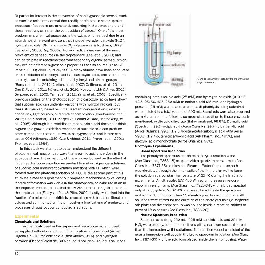
32

Of particular interest is the conversion of non-hygroscopic aerosol, such as succinic acid, into aerosol that readily participate in water uptake processes. Reactions are constantly occurring in the atmosphere and these reactions can alter the composition of aerosol. One of the most predominant chemical processes is the oxidation of aerosol due to an abundance of relevant oxidizers that include hydrogen peroxide (H2O2), hydroxyl radicals (OH), and ozone (O3) (Kawamura & Ikushima, 1993; Lee, et al., 2000; Ray, 2000). Hydroxyl radicals are one of the most prevalent oxidant sources in the troposphere (Lee, et al., 2000) and can participate in reactions that form secondary organic aerosol, which may exhibit different hygroscopic properties than its source (Ansari & Pandis, 2000; Virkkula, et al., 1999). Many studies have been conducted on the oxidation of carboxylic acids, dicarboxylic acids, and substituted carboxylic acids containing additional hydroxyl and alkene groups (Bensalah, et al., 2012; Carlton, et al., 2007; Gallimore, et al., 2011; Gao & Abbatt, 2011; Nájera, et al., 2010; Nepotchatykh & Ariya, 2002; Serpone, et al., 2005; Tan, et al., 2012; Yang, et al., 2008). Specifically, previous studies on the photooxidation of dicarboxylic acids have shown that succinic acid can undergo reactions with hydroxyl radicals, but these studies vary based on initial reactant concentrations, external conditions, light sources, and product composition (Charbouillot, et al., 2012; Gao & Abbatt, 2011; Karpel Vel Leitner & Dore, 1996; Yang, et al., 2008). Although it is established that succinic acid does not exhibit hygroscopic growth, oxidation reactions of succinic acid can produce other compounds that are known to be hygroscopic, and in turn can act as CCN (Albrecht, 1989; Gao & Abbatt, 2011; Prenni, et al., 2001; Twomey, et al., 1984). In this study we attempt to better understand the different photochemical reaction pathways that succinic acid undergoes in the aqueous phase. In the majority of this work we focused on the effect of initial reactant concentration on product formation. Aqueous solutions of succinic acid underwent oxidation reactions with OH which were formed from the photo-dissociation of H2O2. In the second part of this study we aimed to supplement our proposed mechanisms by validating if product formation was viable in the atmosphere, as solar radiation in the troposphere does not extend below 290 nm due to O3 absorption in the stratosphere (Finlayson-Pitts & Pitts, 2000). Lastly, we looked into the fraction of products that exhibit hygroscopic growth based on literature values and commented on the atmospheric implications of products and processes throughout our conducted irradiations.

Experimental Chemicals and Solutions

The chemicals used in this experiment were obtained and used as supplied without any additional purification: succinic acid (Acros Organics, 99%), malonic acid (Sigma Aldrich, 99%), and hydrogen peroxide (Fischer Scientific, 30% aqueous solution). Aqueous solutions

Figure 1: Experimental setup of the Hg immersion lamp irradiations.

containing both succinic acid (25 mM) and hydrogen peroxide (0, 3.12, 12.5, 25, 50, 125, 250 mM) or malonic acid (25 mM) and hydrogen peroxide (25 mM) were made prior to each photolysis using deionized water, diluted to a total volume of 500 mL. Standards were also prepared as mixtures from the following compounds in addition to those previously mentioned: oxalic acid dihydrate (Baker Analyzed, 99.9%), DL-malic acid (Spectrum, 99%), adipic acid (Acros Organics, 99%), tricarballylic acid (Acros Organics, 99%), 1,2,3,4-butanetetracarboxylic acid (Alfa Aesar, >98%), 1,2,4-butanetricarboxylic acid (Ark Pharm, Inc., >95%), and glyoxylic acid monohydrate (Acros Organics, 98%).Photolysis Experiments

Broad Spectrum IrradiationThe photolysis apparatus consisted of a Pyrex reaction vessel

(Ace Glass Inc., 7863-18) coupled with a quartz immersion well (Ace Glass Inc., 7874-35) as shown in Figure 1. Water from an ice bath was circulated through the inner walls of the immersion well to keep the solution at a constant temperature of 20 °C during the irradiation experiments. An ultraviolet (UV) 450 W medium pressure mercury-vapor immersion lamp (Ace Glass Inc., 7825-34), with a broad spectral output ranging from 220-1400 nm, was placed inside the quartz well and warmed up for more than 15 minutes prior to each photolysis. All solutions were stirred for the duration of the photolysis using a magnetic stir plate and the entire set-up was housed inside a reaction cabinet to prevent UV exposure (Ace Glass Inc., 7836-20).

Narrow Spectrum IrradiationSolutions containing 250 mL of 25 mM succinic acid and 25 mM

H2O2 were photolyzed under conditions with a narrower spectral output than the immersion well irradiations. The reaction vessel consisted of the quartz immersion well used in the broad spectrum irradiation (Ace Glass Inc., 7874-35) with the solutions placed inside the lamp housing. Water

33

at room temperature was also circulated through the inner walls of the vessel to prevent condensation inside the chamber and keep the solution within the range of 23-29 °C during the experiment. The quartz well was clamped inside a Rayonet photochamber (Southern N. E. Ultraviolet Co., RPR-100) that included 16 lamps stationed around the exterior walls. The light source consisted of mercury-vapor lamps with a wavelength range of approximately 100 nm centered on a specified wavelength of 254, 300, 419, or 350 nm (Southern N. E. Ultraviolet Co., RPR-2537, RPR-3000, RPR-4190; Hitachi FL8BL-B). Product Derivatization

First, 2 mL aliquots were removed by pipet at various time intervals (t=0, 5, 10, 15, 30, 60, 90, 120 min for broad spectrum irradiations and t=0, 30, 60, 90, 120, 180, 240, 300 min for narrow spectrum irradiations) during the photolysis, of which 1 mL was dispensed into amber GC vials (Thermo Scientific, C4000-82W) and dried overnight under a gentle flow of nitrogen (Praxair, UN1066). Then, 100 µL of pyridine (EMD, >99.0%) and 150 µL of N,O-Bis(trimethylsilyl)trifluoroacetamide + trimethylchlorosilane (BSTFA + TMCS, Thermo Scientific, 99:1) were added to the resulting residue and left to react at room temperature for 1 hour prior to dilution with 1 mL of ethyl acetate (EMD, HPLC grade, >99.8%). Analysis of Derivatized Products

Photolysis products were identified using a NIST database following gas chromatography – mass spectrometry (GC-MS; Hewlett Packard 5890 Series II GC, Hewlett Packard 5971 Series Mass Selective Detector) and confirmed with standards. Products were quantified using gas chromatography – flame ionization detection (GC-FID; Agilent Technologies 6890N Network GC system, Agilent Technologies 7683 AutoSampler, Agilent Technologies 7683 Injector) by comparison to calibration curves. 1 µL samples were injected in the GC-FID equipped with an HP-5 capillary column (5% phenyl methylpolysiloxane, 30 m x 320 µm x 0.25 µm, Agilent) utilizing a splitless injection and a helium flow of 2.2 mL min-1. The temperature program began at 90 °C and held for 3 min, increased to 150 °C at 15 °C min-1 and then to 270 °C at 30 °C min-1 where it was held for 4 min. All products eluted within 15 min. Samples were injected multiple times (3-7), most within 9 hours of derivatization (some up to 19 hours) with no significant change in results.

Results and DiscussionThe main reactive species in our irradiation experiments are hydroxyl

radicals (OH) produced from the photolysis of hydrogen peroxide (H2O2) according to the following reaction:

H2O2 + hv (λ ≤ 360 nm) → 2 OH (1)

An unphotolyzed mixture of 25 mM succinic acid and 25 mM H2O2 was left in the dark for longer than 4 months with no change in composition,

Figure 2: Product formation of major products as a function of photolysis time for a 1:1 mole ratio of a succinic acid and hydrogen peroxide mixture. Error bars represent the standard deviation of three replicate experiments.

demonstrating that the lamp source used in the irradiation experiments was necessary for product formation.

Figure 2 shows composition results from a typical photolysis of a 25 mM succinic acid and 25 mM H2O2 solution as a plot of the concentration as a function of increasing photolysis time over the course of two hours. Succinic acid decays from 23.8 mM to 3.9 mM as the photolysis proceeds, and products such as 1,2,3,4-butanetetracarboxylic acid (BTA) and malonic acid begin to form, which reach a maximum concentration of 0.96 mM and 1.26 mM after 10 and 15 min of photolysis, respectively. Products resulting from the photooxidation of succinic acid eventually decay as the photolysis time proceeds, which indicates that the newly formed products also begin to undergo reactions in the mixture simultaneously with succinic acid. Aqueous oxidation of succinic acid was conducted with various concentrations of H2O2 over the course of two hours. These solutions encompassed different mole ratios of H2O2:SA, namely 0:1, 1:8, 1:2, 1:1, 2:1, 5:1, and 10:1. Therefore, succinic acid solutions in the absence of H2O2 have a ratio of 0:1 and solutions with ten times the amount of H2O2 as succinic acid have a ratio of 10:1. All solutions have a consistent succinic acid concentration (25 mM), and thus the only concentration that varied was H2O2. After analyzing all reaction mixtures, eight compounds were identified following 30 minutes of photolysis, however the products were not all present in the same solution but rather at different concentration ratios. Even still, other unidentified products were present in the photolyzed solutions, though their abundance was much less than the major compounds presented in this work. The physical structures of all identified compounds are illustrated in Figure 3.

34

Figure 4 shows the loss of succinic acid and the formation of reaction products following 30 minutes of photolysis as a function of increasing H2O2 concentration, i.e. H2O2:SA. Photolysis experiments at each H2O2:SA ratio were conducted in duplicates or triplicates, and error bars represent the standard deviation. Eight different products were identified in these experiments, however the concentration as a function of H2O2:SA for 1,2,4-butanetricarboxylic acid is excluded due to a lack of calibration. There are three distinct cases in which specific products are favored in the photooxidation reactions. Products were divided into different categories based on these observations which is shown in Figures 4a, 4b, and 4c, and is based on the ratio of H2O2 to succinic acid at which product concentrations reach a maximum. Figure 4a shows that succinic acid and adipic acid are most prevalent in the absence of H2O2 (H2O2:SA ratio of 0:1). As more H2O2 is added (increasing H2O2:SA ratio), the concentration of succinic and adipic acids decreases following 30 minutes of photolysis. In Figure 4b, 1,2,3,4-butanetetracarboxylic acid reaches a maximum concentration when the H2O2:SA ratio is 2:1, whereas malic acid and tricarballylic acid reach a maximum concentration at a H2O2:SA ratio of 1:2. Since these products are not present in the absence of H2O2, OH is a necessary reactant in their formation. Lastly, Figure 4c shows that photolysis products malonic, oxalic, and glyoxylic acids are most prevalent when the H2O2:SA ratios are 5:1 and 10:1. Oxalic acid and glyoxylic acid reach a maximum concentration at a ratio of 5:1 H2O2:SA, while malonic acid reaches a maximum concentration at a ratio of 10:1 H2O2:SA. Overall,

when sufficient H2O2 was added to the photolysis mixtures such that the concentration was 25 mM succinic acid and 125 mM H2O2 (a ratio of 5:1 H2O2:SA) major products are those that are lower in molecular weight and have fewer carbon atoms than succinic acid (e.g. malonic acid and oxalic acid). In solutions containing 50 mM or less of H2O2, the major products are those that have more carbon atoms than succinic acid and have a larger molecular weight (e.g. tricarballylic acid). Succinic Acid Degredation and Adipic Acid Formation As shown in Figure 4a, the concentration of succinic acid after 30 minutes of photolysis decreases from 16.7 mM to 1.3 mM as H2O2:SA increases from 0:1 to 5:1, and then increases from 1.3 mM to 2.7 mM as H2O2:SA increases from 5:1 to 10:1. The concentration of succinic acid present after 30 minutes of photolysis depends primarily on the concentration of OH in solution produced by the photolysis of H2O2 (Eqn. 1), which is readily photolyzed in both our experimental design and in the atmosphere (Lee, et al., 2000). As OH radicals are formed in the reaction, these radicals can react with succinic acid, thus decreasing its concentration as the reaction proceeds. As the initial concentration of H2O2 increases, succinic acid is more readily oxidized which is indicative of an increase in OH. However, there is an increase in succinic acid following 30 minutes of photolysis between 5:1 and 10:1 H2O2:SA, which may be explained by OH loss processes. If the OH formation rate is consistent at H2O2:SA ratios of 5:1 and 10:1 due to a fixed amount of photons irradiating from the lamp source, an increase in H2O2 provides additional species with which the highly reactive OH

Figure 3: Chemical structures of succinic acid and oxidation products observed throughout the conducted irradiations.

35

can undergo a reaction, thus decreasing the concentration which is available to react with succinic acid. This indicates a slower degradation rate of succinic acid, although there is an increase in the concentration of H2O2. This trend is also seen more predominantly at an earlier time in the photolysis reactions. The concentration of succinic acid after 5 minutes of photolysis decreases from 22.7 mM to 12.9 mM as H2O2:SA increases from 0:1 to 1:1, and then increases from 12.9 mM to 16.6 mM as H2O2:SA increases from 1:1 to 10:1.

Also shown in Figure 4a, adipic acid is most prevalent when a succinic acid solution is irradiated for 30 minutes in the absence of H2O2. Waddell, et al. (1989) demonstrated that succinic acid in the presence of light can react to form products such as adipic acid, methylated glutaric acids, maleic acid, and 2-methylsuccinaldehydic acid. Other products besides adipic acid are formed in our 0:1 H2O2:SA photolysis solutions, however we were unable to identify them with the GC-MS database. Moreover, adipic acid is the predominant product observed in our analysis in solutions irradiated in the absence of H2O2. We propose that succinic acid, a C4 dicarboxylic acid, undergoes decarboxylation in which two radicals are formed. The C1 radical may undergoes further oxidative processes to convert the species to carbon dioxide (CO2), while the C3 radical undergoes a radical mediated termination process with an identical species in order to form adipic acid. Figure 5 demonstrates this possible recombination mechanism in detail. Radical species A is formed in the absence of H2O2, and recombination of two A radicals forms adipic acid. Since adipic acid formation is only observed at low H2O2:SA concentration ratios (less than or equal to 8:1), it is possible that the bond cleavage between the α carbon and carbonyl carbon is still taking place at high H2O2:SA ratios, however, the produced radical species may more readily undergo oxidation processes with OH than in radical recombination mechanisms.

Figure 4: Product formation as a function of increasing hydrogen peroxide concentration in mixtures of succinic acid and hydrogen peroxide at a photolysis time of 30 minutes. a) Succinic acid and adipic acid are most prevalent in the absence of hydrogen peroxide. b) Malic acid, tricarballylic acid, and 1,2,3,4-butanetetra-carboxylic acid are most prevalent at H2O2:SA ratios of 2:1 and 1:2. c) Glyoxylic acid, malonic acid, and oxalic acid most prevalent at H2O2:SA ratios of 5:1 and 10:1.

Figure 5: Radical recombination mechanisms demonstrating the production of two carbon radicals from succinic acid which are formed by light (A) and OH (B). Termination of two radicals either in patterns AA, AB, or BB leads to the formation of adipic acid, 1,2,4-butanetricarboxylic acid, or 1,2,3,4-butanetetracarboxylic acid, respectively.

36

Malic Acid, Tricarballylic Acid, 1,2,4-Butanetricarboxylic Acid, and 1,2,3,4-Butanetetracarboxylic Acid Formation

As shown in Figure 4b, products such as malic acid, tricarballylic acid, and 1,2,3,4-butanetetracarboxylic acid (BTA) are most prevalent after 30 minutes of photolysis in solutions with H2O2:SA ratios between 2:1 and 1:2. Not shown is 1,2,4-butanetricarboxylic acid (due to a lack of calibration) which is most prevalent at a H2O2:SA ratio of 8:1 by observing its change in peak area. In order to form these compounds, OH radicals are necessary in the photolysis, as these products are not present in solutions photolyzed in the absence of H2O2. Other studies have identified the formation of polycarboxylic acids from the irradiation of succinic acid. Karpel Vel Leitner and Dore (1996) identified tricarballylic acid from the OH induced oxidation of succinic acid in deoxygenated solutions. Negron-Mendoza and Albarrán (1993) synthesized BTA from the γ irradiation of succinic acid, along with other minor products including malonic acid, tricarballylic acid, 1,2,4-butanetricarboxylic acid, and H2O2. Previous studies have also suggested that succinic acid undergoes a hydrogen abstraction at the α carbon, which is removed by OH to form water (Charbouillot, et al. 2012; Gao & Abbatt, 2011; Negron-Mendoza & Albarrán, 1993; Yang, et al. 2008). The resulting radical is stabilized by resonance and can undergo further oxidation reactions to form malic acid and malonic acid. Our results demonstrate that these radical species can also undergo recombination mechanisms to form compounds that have a larger molecular mass than succinic acid, which may be a source of oligomer formation in the atmosphere. We propose possible recombination mechanisms for the formation of

1,2,4-butanetricarboxylic acid and BTA as shown in Figure 5. When H2O2 is absent in the photolysis solutions, α−cleavage forms radical species A. Recombination of two A radicals forms adipic acid, as previously stated in earlier sections. In the presence of H2O2, hydrogen abstraction occurs at the α carbon to form radical species B. When two of these radicals undergo radical mediated termination (a maximum occurring at a H2O2:SA ratio of 1:2), BTA is formed. Although theoretical calculations demonstrate that the acidic hydrogen is likely to be abstracted, the formation of BTA in our studies demonstrates that α-hydrogen abstraction is a favorable process (Blanksby & Ellison, 2003; Vimal & Stevens, 2006). The presence of 1,2,4-butanetricarboxylic acid verifies the production of radical species A and B. The formation of this compound reaches a maximum concentration at a H2O2:SA ratio of 8:1, which is a solution that likely includes both radical species A and B, and termination of these species forms the tricarboxylic acid. We also believe that malic acid and tricarballylic acid form through recombination mechanisms which has been reported by Gao and Abbatt (2011) and Karpel Vel Leitner and Dore (1996).Malonic Acid, Oxalic Acid, and Glyoxylic Acid Formation Under photolysis conditions consisting of H2O2:SA ratios of 5:1 and 10:1, the oxidation process of succinic acid to malonic acid was highly favored. Figure 6 shows the photolysis of a 10:1 H2O2:SA solution by the concentration of compounds as a function of photolysis time. Succinic acid completely decays from 25.3 mM over the course of the two hour photolysis, and products such as malonic acid and oxalic acid begin to form. Malonic acid reached a maximum concentration of 11.9 mM after 30 minutes of photolysis. Photooxidation of malonic acid continued to form oxalic acid which reached a maximum concentration of 3.9 mM after 60 minutes of photolysis. In our analysis, we also see the formation glyoxylic and malic acids besides the major products of oxalic and malonic acids; however these compounds are present in small quantities with a concentration of 0.14 mM and 0.13 mM, respectively. In order to verify the production of oxalic acid from malonic acid, we photolyzed a 25 mM malonic acid and 25 mM H2O2 solution which demonstrated the formation of oxalic acid over the course of two hours. Although glyoxylic acid can form from the photolysis of succinic acid as reported by Charbouillot et al, (2012) we do not observe anywhere near the same percentage of glyoxylic acid in our solutions (10:1 H2O2:SA) compared to what they observed. Although their results were obtained from irradiation of solutions with different initial concentrations than in our experimentation (both succinic acid and H2O2), we formed the same products in our 10:1 H2O2:SA solutions indicating we were undergoing an oxidation pathway rather than carbon radical recombination mechanisms as presented in section 3.2. After 30 minutes of photolysis, the time at which malonic acid has reached a maximum concentration, the concentrations of our observed products in the 10:1 H2O2:SA solutions (oxalic, malonic, and glyoxylic acids) represent only 11%, 53%, and

Figure 6: Concentration of major products as a function of photolysis time for a 10:1 mole ratio of a hydrogen peroxide and succinic acid mixture. Error bars represent the standard deviation of three replicate experiments.

37

0.36%, of the amount of succinic acid lost from photooxidation, respectively. These percentages do not add up to 100%. We can only account for 65% of the disappearance of succinic acid in the 10:1 H2O2:SA mixture, compared to the 100% mole balance reported by Charbouillot et al. (2012) throughout their irradiation experiments. After one hour of photolysis, Charbouillot et al. (2012) demonstrated the formation of identical products (oxalic, malonic, and glyoxylic acids,) however they represent 7%, 62%, and 31% of decayed succinic acid, respectively. Unlike our concentrations, they produced more glyoxylic acid than oxalic acid, which are results we cannot replicate in our experimentation. The difference in composition and the loss of succinic acid that is unaccounted for in our reactions may be due to the photon output of our Hg light source compared to Xenon lamps in previous studies. The decay of succinic acid in our photolysis experiments occurs at a faster rate than in other publications. The half life of succinic acid in our 25 mM succinic acid and 250 mM H2O2 solutions is approximately 11 minutes, which is significantly shorter than Gao and Abbatt (2011) (90 minutes), Karpel Vel Leitner and Dore (1996) (100 minutes), and Charbouillot, et al. (2012) (4.6 hours). As the reaction in our experiment proceeds rapidly, this may possibly account for the increase in oxalic acid and lack of glyoxylic acid in our samples compared to the product ratios of Charbouillot, et al. (2012) as the oxidation of glyoxylic acid leads to the formation of oxalic acid (Karpel Vel Leitner & Dore, 1997). The lack of mole balance may also be an indication of other processes that we are unable to measure, such as CO2 evolution, polymer formation, and volatile organic compounds (VOCs) forming during the photolysis. VOCs would evaporate during our sample preparation as we remove water by drying under N2 gas, and these products cannot be analyzed given our current methods and experimentation. Furthermore, as oxalic acid has the largest oxidation rate constant compared to longer chained DCA (Yang, et al., 2008), it may continue to oxidize in the reaction, and following this loss process we can no longer measure carbon containing compounds in order to obtain a mole balance. Mechanisms proposed in the literature for the conversion of succinic acid to malonic and oxalic acids consist of numerous steps and conflict in their intermediates and pathways. Charbouillot et al. (2012) proposed that succinic acid can degrade via two different pathways, either to malonic acid or to oxalic acid through glyoxylic acid. These pathways differ from sequential decarboxylation as they suggest a C4 DCA can form a C2 DCA without first producing the C3 DCA. Gao and Abbatt (2011) identified the production of malonic and malic acids from the photooxidation of succinic acid, however, they were unable to account for oxalic acid in their solutions. They, along with Kawamura and Saguchi (1999), proposed the formation of a malic acid intermediate which is consistent with evidence demonstrating the formation of malonic acid from photooxidation of malic acid by OH (Gao & Abbatt, 2011). Their mechanism, along with that reported by Karpel Vel Leitner and Dore

(1996) who observed malonic and oxalic acid formation, includes oxygen as a necessary reactant based on differing results when the solutions were photolyzed under a purge of N2 gas. In order to better understand the effect of deoxygenation on solutions of succinic acid under both low and high H2O2 conditions, we conducted photolysis reactions of solutions containing 25 mM succinic acid and either 25 mM H2O2 or 125 mM H2O2 under an inert atmosphere (argon purge). Solutions containing succinic acid and H2O2 were purged for 30 minutes prior to photolysis in a Pyrex reaction vessel. A long metal syringe was connected to a metal sparger which provided a generous flow of argon bubbles, and the purge was continued during the irradiation. Neither the high nor low peroxide solutions show any significant difference in succinic acid decay or product formation under an argon purge. This demonstrates that oxygen may not be needed in the degradation pathway. It is possible that not all oxygen (O2) was successfully removed from our solutions which could be contributed to our degassing techniques, or from possible formation of O2 from UV induced reactions of H2O2 or H2O. A reasonable explanation for possible O2 formation is from the cleavage of H2O2 which results in hydroxyl radicals, and then reacts in solution via the following mechanism (Liao and Gurol, 1995):

H2O2 + OH → HO2 + H2O (2)

2 HO2 → H2O2 + O2 (3)

Karpel Vel Leitner and Dore (1996) commented on HO2 formation via the above mechanism (Eqn. 2-3) as it introduces a second atmospherically relevant oxidizer into the reaction mixtures. However HO2 can recombine to reform H2O2, which is then photolyzed to make OH. A byproduct of this reaction is dissolved oxygen which may alter results obtained from deoxygenated samples. Wavelength Dependence In order to verify if our reaction mechanisms are viable in the troposphere, which has a solar actinic flux of λ > 290 nm (Finlayson-Pitts & Pitts, 2000), we also conducted photooxidation reactions of 25 mM succinic acid and 25 mM H2O2 using narrow spectrum irradiations. The lamp sources had an output of approximately 100 nm with wavelengths centered around 254, 300, 350, and 419 nm. As the wavelength of light increased (decreasing energy), the decomposition rate of succinic acid decreased. Similarly, product formation occurred at a slower rate. Compounds identified in the 1:1 H2O2:SA photooxidation reactions at a wavelength of 254, 300, and 350 nm include malonic, malic, tricarballylic, and 1,2,3,4-butanetetracarboxylic acids. In the 419 nm photolysis, the only product we were able to identify was malic acid, however its presence was minimal and only slightly above the detection limit of the GC-FID and GC-MS. These results demonstrate that the

38

previously in earlier sections, the first step in formation is likely through a hydrogen abstraction at the α carbon. In order for this process to occur, OH is a necessary reactant, which shows that our conditions provide enough energy for the dissociation of H2O2. This demonstrates that the majority of products formed in our reactions via the oxidation pathway are independent of wavelength smaller than 350 nm, and these products have been measured and found present in the atmosphere (Fu & Kawamura, 2011).

Atmospheric ImplicationsThe results and reaction mechanisms presented in this experiment

are important for better understanding the dynamics of atmospheric processes as well as the effects they can have on our climate. Aqueous solutions of oxidized organics may continue to undergo further reactions which may alter the chemical composition of the atmosphere. Understanding the composition of these aerosol, and probable reaction products, is essential in understanding how aerosol affect the radiative balance of the earth through both direct and indirect effects. As presented in Part I of this paper, the hygroscopic properties of the oxidized succinic acid aerosol change throughout oxidation, which strongly affects the ability of the aerosol to take up water. Figure 7 shows the relative mole fraction of hygroscopic reaction products identified in our solution as a function of increasing H2O2 concentration after 30 minutes of photolysis. Compounds with a reported deliquescence relative humidity (DRH) greater than 90% were denoted as non-hygroscopic, as listed in Table 1, and are represented in the blue bars (Brooks, et al., 2002; Marcolli, et al., 2004; Moore and Raymond, 2008; Parsons, et al., 2004). Similarly, compounds with a DRH less than 90% or whose growth measurements were conducted on the efflorescence curve were denoted as hygroscopic and these compounds are represented in the red bars (Braban, et al. 2003; Brooks, et al., 2002; Chan, et al., 2008; Marcolli, et al., 2004; Parsons, et al., 2004). Oxalic acid which has conflicting DRH results due to amorphous structures and hydrate formation was included as the green bars (Braban, et al. 2003, Brooks, et al., 2002, Mikhailov et al., 2009). Since 1,2,4-butanetricarboxylic acid does not have a reported DRH and was not calibrated, it is not included in the graph. Literature

Figure 7: Mole fraction of products in solution after 30 minutes of photolysis with varying initial succinic acid to hydrogen peroxide mol ratios. Non-hygroscopic compounds are shown in red, hygroscopic in blue, and compounds with conflicting deliquescence relative humidity (DRH) values due to hydrate formation (oxalic acid) are displayed as green.

Table 1: Literature deliquescence relative humidity values (DRH) used in assigning succinic acid oxidation products as hygroscopic or non-hygroscopic for use in Figure 7.

39

values represent a variety of methods and measurements such as aerosol flow tube-FTIR (AFT), humidified tandem differential mobility analyzer (HTDMA), electrodynamic balance (EDB), vapor pressures over bulk solutions, and optical microscopy.

As shown in Figure 7, as the concentration of H2O2 in the photolyzed solutions increases relative to succinic acid, a larger mole fraction of hygroscopic compounds are formed. This is mostly due to the increase in malonic acid as oxidation to smaller chained DCA takes place when an increased concentration of OH is present in the solution. Likewise, succinic acid, a non-hygroscopic DCA, is consumed in the reaction the more H2O2 is added. This has significant implications for the ability for aerosol to act as CCN as well as overall cloud lifetime. As more hygroscopic particles are present in highly oxidized succinic acid environments, the increase in the amount of particles able to participate in water uptake results in less water being distributed per particle. Overall this is due to a fixed amount of water is present in the atmosphere. Since particles take up less water they are unable to reach a sufficient size where they can rain out, thus promoting a longer cloud lifetime (Jirak, 2006). As clouds remain longer in the atmosphere, they can reflect a greater flux of incoming solar radiation and have an increased negative radiative forcing effect (cooling effect) on the earth and climate system (Albrecht, 1989; Charlson, et al., 1992).

ConclusionsSuccinic acid, a compound known to be non-hygroscopic, does not undergo reactions with hydrogen peroxide in the aqueous phase. However, with the addition of UV light, succinic acid can undergo reactions with OH formed from the dissociation of H2O2 which can produce products that are known to be hygroscopic. The identity of the products produced from the reaction of succinic acid and OH depend on the initial reactant concentrations. This reveals that the radical recombination processes throughout our irradiation experiments are partially based on the availability of reactive species. Radicals are highly reactive and quickly undergo reactions with compounds present within the immediate surroundings. Our results demonstrate that a relative oxidant concentration to aliphatic acid ratio exists (less than 2:1 H2O2:SA), such that in environments with a low OH concentration and H2O2:SA ratios, radical mediated termination is a favorable process over an oxidation pathway leading to CO2 formation. As discussed in this work, the identity and concentration of reaction products varies with initial H2O2 concentration which can affect the composition and properties of atmospheric aerosols. These aerosol can have varying effects on the earth’s climate based on their composition, and thus it is important to understand oxidative loss processes of aerosol in both high and low oxidant concentration environments.

AcknowledgementsSupport for this project was made possible through CSUF Department of Chemistry and Biochemistry start up funds and intramural funds. Special thanks goes to Sergey Nizkorodov at UC Irvine for foundational HPLC analysis which led way to the research conducted in this article. Thank you to the students in the de Lijser and Hudson labs who provided training on the use of the GC and photolysis equipment, as well as aided in experimental data collection. Much gratitude goes to Paula Hudson and Peter de Lijser for their continual support and guidance throughout the duration of this work, and for the time and dedication they contributed towards this project.

References Albrecht, B. A. (1989). Aerosols, cloud microphysics, and fractional cloudiness. Science, 245(4923), 1227-1230.

Ansari, A. S., & Pandis, S. N. (2000). Water absorption by secondary organic aerosol and its effect on inorganic aerosol behavior. Environmental Science and Technology, 34, 71-77.

Bensalah, N., Louhichi, B., & Abdel-Wahab, A. (2012). Electrochemical oxidation of succinic acid in aqueous solutions using boron doped diamond anodes. International Journal of Environmental Science and Technology, 9, 135-143.

Braban, C. F., Carroll, M. F., Styler, S. A., & Abbatt, J. P. D. (2003). Phase Transitions of Malonic and Oxalic Acid Aerosols. Journal of Physical Chemistry A, 107, 6594-6602.

Brooks, S. D., Wise, M. E., Cushing, M., & Tolbert, M. A. (2002). Deliquescence behavior of organic/ammonium sulfate aerosol. Geophysical Research Letters, 19, 23-(1-4).

Blanksby, S. J & Ellison, G. B. (2003). Bond dissociation energies of organic molecules. Accounts of Chemical Research, 36, 255-263.

Carlton, A.G., Turpin, B. J., Lim, H., Altieri, K. E., & Seitzinger, S. (2006). Link between isoprene and secondary organic aerosol (SOA): Pyruvic acid oxidation yields low volatility organic acids in clouds. Geophysical Research Letters, 33, L06822.

Chan, M. N., Kreidenweis, S. N., & Chan, C. K. (2008). Measurements of the hygroscopic and deliquescence properties of organic compounds of different solubilities in water and their relationship with cloud condensation nuclei activities. Environmental Science and Technology, 42, 3602-3608.

40

Charbouillot, T., Gorini, S., Voyard, G., Parazols, M., Brigante, M., Deguillamue, L., Delort, A., & Mailhot, G. (2012). Mechanism of carboxylic acid photooxidation in atmospheric aqueous phase: Formation, fate, and reactivity. Atmospheric Environment, 56, 1-8.

Charlson, R. J., Schwartz, S. E., Hales, J. M., Cess, R. D., Coakley, J. A., Hansen, J. E., et al. (1992). Climate forcing by anthropogenic aerosols. Science, 255(5043), 423-430.

Chebbi, A. & Carlier, P. (1996). Carboxylic acids in the troposphere, occurrence, sources, and sinks: a review. Atmospheric Environment, 24, 4233-4249.

Cruz, C. N., & Pandis, S. N. (2000). Deliquescence and hygroscopic growth of mixed inorganic-organic atmospheric aerosol. Environmental Science and Technology, 34(20), 4313-4319.

Ervens, B., Feingold, G., Frost, G. J., & Kreidenweis, S. M. (2004). A modeling study of aqueous production of dicarboxylic acids: 1. Chemical pathways and speciated organic mass production. Journal of Geophysical Research, 109, D15205.

Falkovich, A. H., Graber, E. R., Schkolnik, G., Rudich, Y., Maenhaut, W., & Artaxo, P. (2005). Low molecular weight organic acids in aerosol particles from Rondonia, Brazil, during the biomass-burning, transition, and wet periods. Atmospheric Chemistry and Physics 5, 781-797.

Feichter, J., & Stier, P. (2012). Assessment of black carbon radiative effects in climate models. Wiley Interdisciplinary Reviews. Climate Change, 3(4), 359-370.

Finlayson-Pitts, B. J., & J. N. J. Pitts. (2000). Chemistry of the Upper and Lower Atmosphere, Elsevier, New York.

Forster, P., Ramaswamy, V., Artaxo, P., Berntsen, T., Betts, R., Fahey, D. W., et al. (2007). 2007: Changes in atmospheric constituents and in radiative forcing. Climate Change 2007: The Physical Science Basis. Contribution of Working Group I to the Fourth Assessment Report of the Intergovernmental Panel on Climate Change. Cambridge, UK and New York, NY, USA: Cambridge University Press.

Fu, P. & Kawamura, K. (2011). Diurnal variations of polar organic tracers in summer forest aerosols: A case study of a Quercus and Picea mixed forest in Hokkaido, Japan. Geochemical Journal, 45, 297-308.

Gallimore, P. J., Achakulwisut, P., Pope, F. D., Davies, J. F., Spring, D. R., & Kalerer, M. (2011). Importance of relative humidity in the oxidative

ageing of organic aerosols: case study of the ozonolysis of maleic acid aerosol. Atmospheric Chemistry and Physics, 11, 12181-12195.

Gao, S. S., & Abbatt, J. P. (2011). Kinetics and mechanism of OH oxidation of small organic dicarboxylic acids in ice: Comparison to behavior in aqueous solution. Journal of Physical Chemistry A, 115, 9977-9986.

Haywood, J., & Boucher, O. (2000). Estimates of the direct and indirect radiative forcing due to tropospheric aerosols: A review. Reviews of Geophysics, 38(4), 513-543.

Hegg, D. A., Gao, S., & Jonsson, H. (2002). Measurements of selected dicarboxylic acids in marine cloud water. Atmospheric Research, 62, 1-10.

Jirak, I. L & Cotton, W. R. (2006). Effect of air pollution on precipitation along the front range of the Rocky Mountains. Journal of Applied Meteorology and Climatology, 45, 236-245.

Kanakidou, M., Seinfeld, J. H., Pandis, S. N., Barnes, I., Dentener, F. J., Facchini, M. C., et al. (2005). Organic aerosol and global climate modelling: a review. Atmospheric Chemistry and Physics, 5, 1053-1123.

Karpel Vel Leitner, N. & Dore, M. (1996). Hydroxyl radical induced decomposition of aliphatic acids in oxygenated and deoxygenated aqueous solutions. Journal of Photochemistry and Photobiology A: Chemistry, 99, 137-143.

Karpel Vel Leitner, N. & Dore, M. (1997). Mechanism of the reaction between hydroxyl radicals and glycolic, glyoxylic, acetic, and oxalic acids in aqueous solution: consequence on hydrogen peroxide consumption in the H2O2/UV and O3/H2O2 systems. Water Research, 31, 1383-1397.

Kaufman, Y. J., Tanre, D., & Boucher, O. (2002). A satellite view of aerosols in the climate system. Nature, 419, 215-223.

Kawamura, K. & Ikushima, K. (1993). Seasonal changes in the distribution of dicarboxylic acids in the atmosphere. Environmental Science and Technology, 27, 2227-2235.

Kawamura, K. & Kaplan, I. R. (1987). Motor exhaust emissions as a primary source for dicarboxylic acids in Los Angeles ambient air. Environmental Science and Technology, 21, 105-110.

Kawamura, K. & Sakaguchi, F. (1999). Molecular distributions of water soluble dicarboxylic acids in marine aerosols over the Pacific Ocean

41

including tropics. Journal of Geophysical Research, 104(D3), 3501-3509.

Kerminen, V., Ojanen, C., Pakkanen, T., Hillamo, R., Aurela, M., & Merilainen, J. (2000). Low-molecular weight dicarboxylic acids in an urban and rural atmosphere. Journal of Aerosol Science, 3, 349-362.

Kitanovski, Z., Grgić, I., & Veber, M. (2011). Characterization of carboxylic acids in atmospheric aerosols using hydrophilic interaction liquid chromatography tandem mass spectrometry. Journal of Chromatography A, 1218, 4417-4425.

Lee, M., Heikes, B. G., & O’Sullivan, D. W. (2000). Hydrogen peroxide and organic hydroperoxide in the troposphere: a review. Atmospheric Environment, 34, 3475-3494.

Loflund, M., Kasper-Giebl, A., Schuster, B., Giebl, H., Hitzenberger, R., & Puxbaum, H. (2002). Formic, acetic, oxalic, malonic, and succinic acid concentrations and their contribution to organic carbon in cloud water. Atmospheric Environment, 36, 1553-1558.

Lohmann, U. & Feichter, J. (2005). Global indirect aerosol effects: a review. Atmospheric Chemistry and Physics, 5, 715-737.

Marcolli, C., Luo, B, & Peter, T. (2004). Mixing of the Organic Aerosol Fractions: Liquids as the Thermodynamically Stable Phases. Journal of Physical Chemistry A, 108, 2216-2224.

Mikhailov, E., Vlasenko, S., Martin, S. T., Koop, T., & Poschl, U. (2009). Amorphous and crystalline aerosol particles interacting with water vapor: conceptual framework and experimental evidence for restructuring, phase transitions and kinetic limitations. Atmospheric Chemistry and Physics, 9, 9491-9522.

Moore, R. H. & Raymond, T. M. (2008). HTDMA analysis of multicomponent dicarboxylic acid aerosols with comparison to UNIFAC and ZSR. Journal of Geophysical Research, 113, 1-15.

Nájera, J. J., Percival, C. J., & Horn, A. B. (2010). Kinetic studies of the heterogeneous oxidation of maleic and fumaric acid aerosols by ozone under conditions of high relative humidity. Physical Chemistry Chemical Physics, 12(37), 11417-11427.

Narukawa, M. & Kawamura, K. (1999). Distribution of dicarboxylic acids and carbon isotopic compositions in aerosols from 1997 Indonesian forest fires. Geophysical Research Letters, 26(20), 3101-3104.

Negrón-Mendoza, A. & Albarrán G. (1993). Synthesis of

1,2,3,4-butanetetracarboxylic acid from the irradiation of aqueous succinic acid. Radiation Physics and Chemistry, 42, 973-976.

Nepotchatykh, O. V. & Ariya, P. A. (2002). Degradation of dicarboxylic acids (C2-C9) upon liquid-phase reactions with O3 and its atmospheric implications. Environmental Science and Technology, 36, 3265-3269.

Osborne, S. R., Baran, A. J., Johnson, B. T., Haywood, J. M., Hesse, E., Newman, et al. (2011). Short-wave and long-wave radiative properties of Saharan dust aerosol. Quarterly Journal of the Royal Meterological Society, 137, 1149-1167.

Parsons, M. T., Mak, J., Lipetz, S. R., & Bertram, A. K. (2004). Deliquescence of malonic, succinic, glutaric, and adipic acid particles. Journal of Geophysical Research, 109, D06212.

Prenni, A. J., DeMott, P. J., Kreidenweis, S. M., Sherman, D. E., Russell, L. M., & Ming, Y. (2001). The effects of low molecular weight dicarboxylic acids on cloud formation. Journal of Physical Chemistry A, 105, 11240-11248.

Ray, M. B. (2000). Photodegradation of the volatile organic compounds in the gas phase: A review. Developments in Chemical Engineering and Mineral Processes, 8(5/6), 405-439.

Sellegri, K., Gourdeau, J., Putaud, J. P., & Despiau, S. (2001). Chemical composition of marine aerosol in a Mediterranean coastal zone during the FETCH experiment. Journal of Geophysical Research, 106, 12,023-12,037.

Serpone, N., Martin, J., Horikoshi, S., & Hidaka, H. (2005). Photocatalyzed oxidation and mineralization of C1-C5 linear aliphatic acids in UV-irradiated aqueous titania dispersions-kinetics, identification of intermediates, and quantum yields. Journal of Photochemistry and Photobiology A: Chemistry, 169, 235-251.

Southern New England Ultraviolet Company. (2002). Spectral distribution of irradiance density for the UV lamps. http://www.rayonet.org/graphscharts.htm. (March 3, 2013).

Tan, Y., Lim, Y. B., Altieri, K. E., Seitzinger, S. P., & Turpin, B. J. (2012). Mechanisms leading to oligomers and SOA through aqueous photooxidation: insights from OH radical oxidation of acetic acid and methylglyoxal. Atmospheric Chemistry and Physics, 12, 801-813.

42

Twomey, S. A., Piepgrass, M., & Wolfe, T. L. (1984). An assessment of the impact of pollution on global cloud albedo. Tellus, 36B, 356-366.

Vimal, D. & Stevens, P.S. (2006). Experimental and theoretical studies of the kinetics of the reactions of OH radicals with acetic acid, acetic acid-d3 and acetic acid-d4 at low pressure. Journal of Physical Chemistry A, 110, 11509-11516.

Virkkula, A., Van Dingenen, R., Raes, F., & Hjorth, J. (1999). Hygroscopic properties of aerosol formed by oxidation of limonene, α-pinene, and β-pinene. Journal of Geophysical Research, 104(D3), 3596-3579.

Waddell, T. G., Geevarghese, S. K., Henderson, B. S., Pagni, R. M., & Newton, J. S. (1989). Chemical evolution of the citric acid cycle: sunlight and ultraviolet photolysis of cycle intermediates. Origins of Life and Evolution of the Biosphere, 19, 603-607.

Wise, M. E., Surratt, J. D., Curtis, D. B., Shilling, J. E., & Tolbert, M. A. (2003). Hygroscopic growth of ammonium sulfate/dicarboxylic acids. Journal of Geophysical Research, 108(D20), 4638.

Yang, L. M., Yu, L. E., & Ray, M. B. (2008). Potential photooxidation pathways of dicarboxylic acids in atmospheric droplets. American Journal of Environmental Sciences, 4(5), 462-466.

Yang, L., Ray, M. B., & Yu, L. E. (2008). Photooxidation of dicarboxylic acids--Part II: Kinetics, intermediates, and field observations. Atmospheric Environment, 42, 868-880.

Zardini, A. A., Sjogren, S., Marcolli, C., Krieger, U. K., Gysel, M., Weingartner, E., et al. (2008). A combined particle trap/HTDMA hygroscopicity study of mixed inorganic/organic aerosol particles. Atmospheric Chemistry and Physics, 8, 5589-5601.

43

Aqueous Phase Oxidation of Succinic Acid by Hydroxyl Radicals. Part I. Hygroscopic Behavior of the Reaction Products


Aaron Ninokawa, Shaun Cook, Trent Northen, Paula K. Hudson

AbstractAtmospheric particles (aerosol) have been identified as important factors in understanding climate change based on their ability to act as cloud condensation nuclei (CCN). The extent to which aerosol affect climate is determined, in part, by their hygroscopic properties, how they take up water vapor. A branch of chemical compounds, the dicarboxylic acids, are common components of atmospheric aerosol and have vastly different hygroscopic properties where some compounds readily take up water and others do not. Further, the particles can react with chemicals in the atmosphere producing new products, possibly having different hygro-scopic properties than the original particles. In this study, the hygroscopic properties of dicarboxylic acid aerosol were measured with a humidified tandem differential mobility analyzer (HTDMA) and compared to reac-tion products resulting from the light induced oxidation (photo-oxidation) of succinic acid, a non-hygroscopic dicarboxylic acid. After reaction with hydroxyl radicals, produced via photolysis of the hydrogen peroxide in solution, hygroscopic products are formed. The reaction conditions were examined by comparing solutions with varying hydrogen peroxide:succinic acid concentration ratios. Major reaction products were determined with gas chromatography-flame ionization detection (GC-FID) and GC-mass spectrometry (GC-MS). Comparison of growth curves to Zdanovskii-Stokes-Robinson (ZSR) predictions suggests that the hygroscopic properties of many of the product mixtures are largely independent of the hygroscopicity of the individual components. This study provides a frame-work for future investigations to fully understand and predict the role of chemical reactions in altering atmospheric conditions that affect climate.

IntroductionAerosol particles suspended in the atmosphere affect the radiative balance of the earth and, in turn, affect climate. They can directly interact with incoming solar radiation and outgoing terrestrial radiation through scattering or absorption and they can interact with water vapor by taking up or releasing water based on the ambient water vapor concentration, or relative humidity (Albrecht, 1989; Charlson, et al., 1992; Haywood & Boucher, 2000; Kaufman, et al., 2002; Lohmann & Feichter, 2005). The tendency of particles to interact with water vapor, described as the

hygroscopic properties of aerosol, also relates to the formation of clouds, which can also scatter and absorb radiation (Albrecht, 1989; Charlson, et al., 1992; Haywood & Boucher, 2000; Kaufman, et al., 2002; Lohmann & Feichter, 2005), and cloud drying/processing (Kanakidou, et al., 2005). Thus, aerosol can indirectly affect the radiative balance of the earth. It is difficult to quantify the indirect effects of aerosol on climate so the magnitude of these effects is poorly understood (Forster, et al., 2007). One class of common aerosol is the short chain (C2-C9) α,ω−dicarboxylic acids (DCA) constituting up to sixteen percent of aerosol organic carbon mass in some areas (Kawamura & Sakaguchi, 1999). DCA are characterized by having a carboxylic acid functional group on each end of a straight carbon chain. They are produced naturally by biomass burning (Narukawa & Kawamura, 1999) and anthropogenically by automobile exhaust (Kawamura & Kaplan, 1987) or as secondary products through photochemical processes (Kawamura & Ikushima, 1993). The hygroscopic properties of DCA have been well studied—for example, succinic (C4) or adipic acid (C6) particles are known to be non-hygroscopic (they do not readily take up water), whereas particles composed of malonic (C3) or glutaric acid (C5) are hygroscopic (Prenni, et al., 2001; Cruz & Pandis, 2000; Parsons, et al., 2004; Wise, et al., 2003; Zardini, et al., 2008). Further, reactions commonly take place in the atmosphere and aerosol composition and resulting hygroscopic properties may change (Virkkula, et al., 1999). One possible reaction that can occur is the oxidation by hydroxyl radicals. Hydroxyl radicals are prevalent atmospheric oxidizers and have been studied extensively for their ability to remove environmental pollutants (Goncharuk, et al., 2010; Ray, 2000) and have the ability of converting non-hygroscopic particles, like succinic acid, to products whose components are complex mixtures of hygroscopic DCA (Gao & Abbatt, 2011; Kawamura & Ikushima, 1993; Yang, Ray, & Yu, 2008). The conversion of non-hygroscopic compounds to hygroscopic products in aerosol may have important implications for the radiative balance of the atmosphere. Several studies have previously examined the reaction of DCA with hydroxyl radicals. Some of these studies

44

have identified product composition, calculated reaction rates, and proposed potential reaction mechanisms often speculating about the potential atmospheric implications of reactions with hydroxyl radicals or other atmospheric oxidizers (Ansari & Pandis, 2000; Gao & Abbatt, 2011; Yang, Ray, & Yu, 2008). However, very few studies have described the atmospheric behavior of the product mixtures of photo-oxidation reactions (Virkkula et al., 1999). While there are several theoretical or semi-empirical models that can be used to approximate aerosol hygroscopic properties given the composition and behavior of the individual components (e.g. Zdanovskii-Stokes-Robinson), these models are often not sufficient in fully describing hygroscopic growth of mixtures, especially those made up of DCA (Moore & Raymond, 2008). In this study, we describe the aqueous phase reaction of succinic acid (SA), a non-hygroscopic DCA, with hydroxyl radicals, produced from the photolysis of hydrogen peroxide (H2O2). Performing this reaction in the aqueous phase mimics the reaction that would take place in atmospheric water droplets. Presented here is a detailed examination of factors that shape the outcome of this reaction, in particular, the amount of H2O2 initially present. Gas chromatography was used to identify and quantify the products (described in detail in part II of this work). The focus of this work was to observe and quantify the hygroscopic properties of the reaction product mixtures as a function of relative humidity using a humidified tandem differential mobility analyzer (HTDMA). Our goal was to not only determine the hygroscopic growth behavior of the product aerosol, but also to determine the extent to which the Zdanovskii-Stokes-Robinson model accurately predicts the growth of the product mixture.

ExperimentalIn this study, the hygroscopic properties of product solutions were observed as a function relative humidity (RH) and hydrogen peroxide:succinic acid ratio (H2O2:SA). Sample Preparation. Reactant solutions contained 25 mM succinic acid (Acros, 99%) and various concentrations of hydrogen peroxide (Fisher Scientific, 30%). Table 1 shows the H2O2:SA concentration ratios of the samples studied. All solutions were photolyzed for 30 minutes.

Photo-oxidation reactions. Reactions were carried out in a 500 mL glass reaction vessel (Ace Glass Inc., 7863-18) with a quartz immer-sion well (Ace Glass Inc., 7874-35) that housed a 450 W mercury vapor immersion lamp (Ace Glass Inc., 7825-34). An external pump cycled water through the immersion well and maintained a consistent reaction temperature of 25˚C. Photolysis reactions took place in a safety reaction cabinet (Ace Glass Inc., 7836-20) to protect the handlers from UV expo-sure during sample preparation. Hygroscopic measurements. A humidified tandem differential mobility analyzer (HTDMA) was used to determine the hygroscopic properties of the samples as a function of relative humidity (RH) as shown in the sche-matic in Figure 1. The HTDMA technique is well established, (e.g. Brech-tel & Kreidenweis, 2000) and has been used extensively to measure the hygroscopic properties of various organic compounds and their mixtures (Moore & Raymond, 2008; Marcolli, et al., 2004; Prenni, et al., 2001) A polydisperse distribution of aerosol were generated with a constant output atomizer (TSI Inc., Model 3076) and dried with a series of silica diffusion dryers to less than 6% RH. The dry aerosol passed through an electrostatic classifier (EC) (TSI Inc., Model 3080) and a differential mobility analyzer (DMA1) (TSI Inc., Model 3081) where the particles were charged and size-selected at 100 nm according to their electrostatic mobility. The monodisperse particles were exposed to relative humidity in one of two different mixing volumes—a Nafion® gas dryer (Perma Pure, MD-110-144P-4) or a cylindrical acrylonitrile-butadiene-styrene (ABS) chamber. In the Nafion® mixing volume, humidified air was passed countercurrent to the aerosol flow separated by a Nafion® membrane. There was no direct mixing of the humidified air and the aerosol flow; only water vapor passed through the Nafion® membrane. In the ABS mixing volume, humidified air was injected directly into the aerosol flow. With both humidification systems, the RH of the humidified air was carefully controlled by mixing different ratios of wet air and dry air with mass flow controllers (Allicat Scientific, MC-5SLPM-D). The residence time of the

[H2O2] [succinic acid] [H2O2]:[succinic acid] 0.00 25 0:1 3.13 25 1:8 12.5 25 1:2 25.0 25 1:1 50.0 25 2:1 125 25 5:1 250 25 10:1

Figure 1. Schematic of the HDMA system used in this study.

Table 1. Concentrations (mM) of succinic acid and hydrogen peroxide in each solution prepared in this study.

45

aerosol in the Nafion® mixing volume was approximately 6.8 seconds while the residence time in the ABS mixing volume was approximately 64 seconds. A calibration of both mixing volumes with ammonium sulfate and sodium bromide yielded that there was no difference in the deliquescence relative humidity, the RH at which dry particles take up water to become liquid particles or the absolute amount of growth of particles after deliquescence. After humidification, the size distribution of the particles was measured using a scanning mobility particle sizer (SMPS) which consists of an EC and DMA (DMA2) coupled to a condensation particle counter (CPC). As with the aerosol humidity, the RH of DMA2 was controlled by combining flows of wet and dry air in specific ratios. The relative humidity levels of the aerosol mixing volume and the DMA2 column were maintained to within 2% RH of each other as suggested by Brechtel and Kreidenweis (2000). Figure 2 shows an example of the resulting size selected size distribu-tion measured with the SMPS for ammonium sulfate particles generated from a 1 wt % solution at 0 % and 80 % RH. A narrow distribution of particle sizes is observed for the ammonium sulfate aerosol at 0% RH centered at 100 nm, the diameter at which it was size selected. Peaks appearing at 145 and 195 nm are artifacts of aerosol charging (“ghost peaks”) and are ignored. After exposure to 80% RH, the peak diameter shifts to 140 nm due to the uptake of water by the ammonium sulfate aerosol. Peak diameters were determined by a Gaussian fit to the mea-sured size distribution at the corresponding equilibrated relative humid-ity. Hygroscopic activity, the growth factor (GF), is quantified by the growth of the particle, the particle diameter at a given relative humidity (DRH) relative to the dry particle diameter (Do) as shown in equation 1.

(Eqn. 1)

The ability of the particle to effloresce, or to dry completely, in our system can be gauged by the initial dry particle diameter. For example, because the diameter of ammonium sulfate in Figure 2 was 100 nm when it was size selected at 100 nm, it indicates that the particles were dry prior to size selection. When the D0 was significantly smaller than the size select diameter, this indicated that the compound did not completely dry before DMA1 and the particles experienced continued water loss after size selection.

Results and DiscussionFigure 3 shows the calculated growth factor as a function of relative humidity for the product solutions created by the 30 minute photolysis of the mixtures indicated in Table 1 for a) SA without H2O2, b) 1:8, 1:2, 1:1, and 2:1 H2O2:SA reaction product aerosol, and c) 5:1 and 10:1 H2O2:SA reaction product aerosol. Figure 3a shows a consistent growth factor (GF) of one from 0-96% RH for succinic acid photolyzed for 30 minutes. Because the value of the

Figure 2. Particle size distributions for dry (0% RH, black circles) and wet (80% RH, grey circles) ammo-nium sulfate ((NH4)2SO4) selected at 100 nm. For each distribution, the maximum of the largest peak, as determined with a Gaussian fit, was recorded as the average particle diameter for ammonium sulfate at the indicated RH. Additional peaks are experimental artifacts of aerosol charging and were ignored.

Figure 3. Hygroscopic growth curves for a) succinic acid, b) 1:8, 1:2, 1:1, and 2:1 H2O2:SA, and c) 5:1 and 10:1 H2O2:SA. Growth factor less than one are indicative of microstructure rearrangement (discussed in text).

GF = DRH

D0

46

growth factor did not change with increasing RH, no change in diameter was observed and no water was taken up by the SA particles. The initial dry peak diameter, after size selection at 100 nm, varied between 96 and 97 nm suggesting that these products dried completely before size selection. The growth curves for 1:8, 1:2, 1:1, and 2:1 H2O2:SA product solution aerosol are shown in Figure 3b. As relative humidity increased from 10 to 30% RH, the growth factor decreased from one to a minimum value of 0.90. Above 30% RH, the growth factor begins to increase to a maximum value of 1.08 at 90% RH showing that addition of just a small amount of hydrogen peroxide to this reaction can cause a measurable difference in the hygroscopicity of the reaction product aerosol. Growth factors less than one have been observed in the HTDMA system before. Mikhailov et al. (2004) proposed two explanations for this phenomenon referred to as microstructure, or crystal, rearrangement. The first is error associated with non-spherical particle sizing. The theory of size selection in the DMA assumes all particles are spherical. However, non-spherical particles will experience an altered mobility leading to an overestimation of the true particle size. Exposure to humidity smoothens the particles to a more spherical shape leading to a better estimation of aerosol size in DMA2 re-sulting in an apparent decrease in particle diameter (growth factor) with increasing relative humidity. The other possibility is that the particles are porous. The introduction of humidity then causes aerosol structure col-lapse leading to an actual smaller particle diameter measured in DMA2. Therefore, it is likely that, even though particle diameters were decreas-ing, the particles were likely taking up monolayer amounts of water. The initial diameters of these solutions were between 96 and 99 nm indicat-ing the aerosol readily dried prior to size selection. Figure 3c shows the hygroscopic growth curves for the 5:1 and 10:1 H2O2:SA reaction product aerosol. As previously observed for the 1:8, 1:2, 1:1, and 2:1 H2O2 solutions, the growth factor for the 5:1 H2O2:SA aerosol gradually decreased to a minimum GF of 0.90 at 15% RH. Particles then grew to a maximum GF of 1.5 at 90% RH. However, for the 10:1 solution, an initial decrease in growth factor was not observed, rather, particles grew continuously to a maximum GF of 2.0 at 90% RH. Continuous

growth of this magnitude is typical of hygroscopic compounds that have not dried completely (Marcolli, et al., 2004; Moore & Raymond, 2008; Prenni, et al, 2001) suggesting that the reaction products of the 5:1 and 10:1 H2O2:SA solutions likely had more hygroscopic products than solu-tions with a smaller relative amount of H2O2. This is further supported by the fact that aerosol generated from 5:1 and 10:1 H2O2:SA reaction products had initial dry diameters of 71 nm and 48 nm, respectively. An initial dry diameter smaller than the initial size selected particle diameter suggests that particles were still wet when size selected and then con-tinued to dry, decreasing in size, until measured again in DMA2. Alter-natively, the reaction products may have such high vapor pressures that the reaction products are evaporating prior to being measured by DMA2 resulting in an observed decrease in particle diameter. Microstructure rearrangement was observed for the 5:1 H2O2:SA reaction products of similar magnitude to the 1:8-2:1 H2O2:SA solutions (minimum GF of 0.90) but reached a minimum at 15% RH rather than the previously observed 30% RH and started immediately rather than the previously observed de-lay to 10 %RH (Figure 3b)This behavior is consistent with the assumption that the 5:1 H2O2:SA, and the 10:1 H2O2:SA, reaction products did not dry completely suggesting an increase in hygroscopicity with increased oxida-tion by hydroxyl radicals. Although our results suggest an increase in the formation of hygro-scopic products as a result of photo-oxidation, in order to predict the behavior of mixtures of products it is necessary to identify the compo-nents responsible for the increased hygroscopicity. Gas chromatography (GC) with mass spectrometry (MS) and flame ionization detection (FID) was used to identify and quantify, respectively, the compounds present in each of the product mixtures (see Part II of this study for more details). Table 2 lists the major compounds identified in the product mixtures and the calibrated concentrations of each including products such as adipic acid when no H2O2 was present; malic acid, 1,2,3,4-butanetetracarbox-ylic acid (succinic acid dimer), and tricarballylic acid forming at H2O2:SA ratios between 1:8 and 2:1; and malonic acid and oxalic acid forming at H2O2:SA ratios greater than 5:1. Figure 4 shows the individual growth curves of a) succinic, adipic, and oxalic acids, b) malic and tricarballyic

[H2O2]:[succinic acid] oxalic malonic succinic malic adipic tricarballylic succinic dimer*0:1 0.06 0.21 16.9 0.03 0.85 0.00 0.101:8 0.06 0.24 16.2 0.05 0.53 0.03 0.221:2 0.08 0.54 12.8 0.15 0.03 0.12 0.891:1 0.15 1.25 7.13 0.21 0.02 0.21 0.742:1 0.40 3.69 4.09 0.25 0.02 0.28 0.495:1 7.34 10.00 1.33 0.13 0.00 0.00 0.1010:1 2.56 11.90 2.75 0.08 0.00 0.00 0.10 *1,2,3,4-butanetetracarboxylic acid

Table 2. Acid product concentrations (mM) present in the solutions prepared in this study.

47

acid and 1,2,3,4-butanetetracarboxylic acid (succinic acid dimer), and c) malonic acid—products identified by GC-MS. As has been observed previ-ously, succinic and adipic (Moore & Raymond, 2008; Prenni, et al., 2001; Sjogren, et al., 2007) acids show no water uptake (GF = 1 across all RHs) and oxalic acid exhibits growth consistent with the predicted growth of oxalic acid dihydrate from a thermodynamic model growing to 1.25 GF at 90% RH (Prenni, et al., 2001; Mikhailov, et al., 2004). The growth curves of malic acid and malonic acid are also consistent with previous studies reaching a GF of 1.25 at 95% RH for malic acid and 2.25 GF at 90% RH for malonic acid (Peng, et al., 2001, Prenni, et al., 2001). To the best of our knowledge the hygroscopic properties of tricarballylic acid and the succinic acid dimer have not been measured with a TDMA and this is the first reported instance. When size selected at 100 nm the initial diameters for adipic and succinic acids were 96 and 94 nm respectively, indicating that these particles easily dry. Small deviations from 100 nm

were attributed to particle evaporation and not the drying capability of the compounds. The initial diameter of oxalic acid was 91 nm while malic acid, tricarballylic acid, and the succinic acid dimer were found to have initial diameters of 98 nm even though they all exhibited continuous growth. This may suggest the presence of amorphous semi-solids that un-dergo gradual water uptake instead of the rapid deliquescence observed by dry particles (Mikhailov, et al. 2009). The initial diameter for malonic acid was the furthest from the size selected diameter at 40 nm indicating that malonic acid did not readily dry. In order to determine the effect of the individual components in the product mixtures on the overall hygroscopic behavior of the aerosol, we incorporated the Zdanovskii-Stokes-Robinson (ZSR) model into our study. The Zdanovskii-Stokes-Robinson relationship has been used to predict the growth of particles by assuming the each of the particle components take up water independently of the other components in the mixture (Cruz & Pandis, 2000; Stokes & Robinson, 1966). Under this assump-tion, the growth factor of a mixture of compounds can be described at a particular RH by (Eqn. 2)

where GFmixture is the predicted growth factor for the mixed particle, ∈i is the volume fraction of the ith component, GFi is the experimental growth factor of the ith component at the given RH, and z is the total number of components in the particle (Moore & Raymond, 2008). The volume frac-tion of each component (∈i) was calculated using the GC-FID determined concentrations along with molar masses and densities obtained from the compound manufacturers. To calculate the ZSR model throughout the entire range of RHs, the HTDMA growth factor curves for each individual component were fit by a second order polynomial with the formGF= A + B(RH) + C(RH)2. The fit coefficients and other parameters used for calculating the ZSR models are shown in Table 3. Figure 5 compares the ZSR-predicted growth curves to the observed growth curves for the product solutions created by the 30 minute photolysis of the mixtures from Table 1 combined with the data from Figure 3 for a) SA without H2O2, b) 1:8, 1:2, 1:1, and 2:1 H2O2:SA product

oxalic 90.04 1.895 1.01E+0 -3.29E-03 6.16E-05malonic 104.06 1.619 9.68E-01 7.15E-03 7.28E-05succinic 118.09 1.572 9.99E-01 2.16E-04 -1.54E-06malic 134.06 1.601 9.98E-01 1.53E-03 1.09E-05adipic 146.14 1.36 9.99E-01 5.54E-04 -4.60E-06tricarballylic 176.12 1.574 9.99E-01 9.87E-04 1.44E-05succinic dimer 234.16 1.674 9.98E-01 1.73E-03 6.28E-06

Figure 4. Growth curves of pure components identified in the reaction product mixtures for a) succinic acid, adipic acid, and oxalic acid b) malic acid, tricarballylic acid, and the succinic acid dimer (1,2,3,4-butanetetracarboxylic acid) and c) malonic acid.

GFmixture = ∑ ∈i • GFi( )i =1

3

Table 3. Table of fit parameters for component growth curves and additional parameters used to calculate ZSR models.

Acid Product Molar Mass DensityGF Fit Parameters

A B C

48

solution aerosol, and c) 5:1 and 10:1 H2O2:SA solution aerosol. Figure 5a shows that the ZSR model for photolyzed succinic acid predicted a GF of near one at all RHs and is within 4% of the observed GF between 0% RH and 90% RH. The model predicted only slight growth, not enough to indicate a distinct difference from a growth factor of one at RHs less than 90% RH. Above 90% RH, though, slight growth is predicted (1.047 GF at 96% RH). Based on factors discussed in Part II of this work, it is likely that only succinic and adipic acids were present in this solution. The prediction of slight growth is likely due to errors inherent in the calibrations for determining the concentrations. In Figure 5b, the ZSR-predicted growth curves are shown for the 1:8, 1:2, 1:1, and 2:1 H2O2:SA solution aerosol compared to the observed growth curves for these aerosol. Zdanovskii-Stokes-Robinson models for these four mixtures indicated that aerosol generated from each solu-tion should exhibit dramatically different water uptake curves from each

other. At 90% RH, the ZSR model predicted GFs of 1.05, 1.12, 1.30, and 1.65 for the 1:8, 1:2, 1:1, and 2:1 H2O2:SA product aerosol, respectively. According to the predictions, hygroscopic growth should be increasing with increasing relative H2O2 concentration. But, the observed growth curves are within 0.04 GF of each other, reaching a maximum GF of 1.06 at 90% RH. Similar observed growth for different mixtures with com-pounds of dissimilar chemistry has been previously observed for mixtures containing 5-10 different DCAs (Moore & Raymond, 2008); complex DCA mixtures tend to exhibit similar hygroscopic growth regardless of individual component properties. Additionally, the ZSR predicted growth was greater than the observed amount of growth. This, too, was observed by Moore and Raymond (2008)—they found that growth curves of DCA mixtures were typically over-predicted by ZSR models based on individual component hygroscopicity. One of the assumptions of the ZSR model is that each component takes up water independent of other compounds in solution (Stokes & Robinson, 1966). It does not account for solute interactions or surface effects caused by sequential drying of the particle components, which may both be occurring in the 1:8, 1:2, 1:1, 2:1, 5:1 H2O2:SA solutions. Additionally, there could be other, unidentified com-pounds in solution that have an unknown effect on the uptake of water. Not all compounds present in the mixtures were used in the model due to limitations associated with identifying and quantifying components. An-other possibility, suggested by Sjogren et. al. (2007), is that the residence time is insufficient for complete equilibration, leading to a decreased observed GF relative to the predicted GF. This is not likely because we used two mixing volumes of very different residence times and there was no discernable difference between the growth curves obtained from each (data not shown) though there is the possibility that residence times significantly greater than 64 seconds are needed. The growth of photolyzed 5:1 H2O2:SA mixture, shown in Figure 5c, was also over-predicted by the ZSR model, possibly for reasons men-tioned above. However, the growth of this mixture was different from the 1:8, 1:2, 1:1, and 2:1 H2O2:SA product mixtures. There are fewer compounds in this solution (mostly succinic, oxalic, and malonic acids). This is still supported by the conclusions of Moore and Raymond (2008). Because there were fewer components in this solution, the growth pre-dicted by the ZSR model was more dependent on the characteristics of the individual components of the mixture. The only reaction product with good agreement between the mea-sured and predicted values is from the 10:1 H2O2:SA reaction product, as shown in Figure 5c. Composition data shows that this reaction mixture was nearly 60% malonic acid by volume. In fact, the growth of malonic acid was very similar to the model and to the mixture and is also shown in Figure 5c for comparison. However, as expected, the growth predicted by the model is slightly inhibited compared to malonic acid, likely due to the presence of other compounds, like succinic acid and oxalic acid, which are not as hygroscopic.

Figure 5. Zdanovskii-Stokes-Robinson (ZSR) predictions of hygroscopic growth curves for a) succinic acid, b) 1:8, 1:2, 1:1, and 2:1 H2O2:SA, and c) 5:1 and 10:1 H2O2:SA. Observed growth curves and growth curve for malonic acid (c) are included for reference. Mixtures exhibiting crystal rearrangement are not well predicted by the ZSR models.

49

The main factor explaining the discrepancy between the ZSR models and the observed growth could be the presence of microstructure rear-rangement. The calculations of the ZSR models involve knowing the vol-ume fraction of each component. However, the presence of microstruc-ture rearrangement indicates that the particles are likely porous or have a shape that causes the DMA1 to miscalculate the aerosol size. Equation 2 shows that the predicted growth factor is directly related to the volume fraction of each component which is calculated on the assumption that each aerosol is a solid, dry sphere. But, the presence of microstructure rearrangement suggests that the particles are either porous or that there sizes are being over-estimated leading to an overestimation of the vol-ume fraction and therefore, the GF. This theory is supported by our obser-vations. All mixtures exhibiting microstructure rearrangement (1:8 – 5:1 H2O2:SA) were over-predicted by the ZSR model whereas mixtures lacking an apparent rearrangement (10:1 H2O2:SA) were much better predicted by the ZSR relation. This would potentially explain why the ZSR models over-predicted the 1:8-2:1 H2O2:SA solutions but would still not account for difference in the magnitude of the over-prediction for these mixtures suggesting that there are more interactions in the mixture beyond micro-structure rearrangement determining the growth of the product aerosol.

Conclusions and Atmospheric ImplicationsSuccinic acid is a non-hygroscopic compound; it does not readily take up water. Without the presence of H2O2 no growth is observed because lon-ger chain, similarly non-hygroscopic, reaction products are formed (see Part II). The addition of an atmospherically relevant oxidizer, H2O2, and 30 minutes of exposure to UV light produced aerosol with hygroscopic behavior. As the relative concentration of H2O2 is increased, hygroscopic reaction products begin to form. However, the concentration of succinic acid is still sufficient enough to nucleate the aerosol. Once the relative concentration of H2O2 exceeds five times that of succinic acid the con-centration of hygroscopic components (e.g. malonic and oxalic acids) are sufficiently large, and the succinic acid concentration sufficiently small, such that the nucleation of succinic acid is unable to create a critical germ large enough to effectively crystallize the hygroscopic compounds. Observed growth does not match that predicted by the ZSR calculations which typically over-predict the hygroscopic growth. This could be a result of insufficient residence time in the humidification chamber, unidenti-fied compounds in the product mixture, or surface effects resulting from sequential nucleation of the components in solution. The conversion of non-hygroscopic compounds to hygroscopic prod-ucts can have large implications in cloud processes. If particles that nor-mally would not take up water are converted to particles that do, formerly non-hygroscopic aerosol would start competing with other hygroscopic aerosol for the available atmospheric water; with limited water vapor availability and an increased concentration of hygroscopic particles, each particle will not be able to take up enough water to form rain droplets

causing cloud lifetime to increase accompanied by decreased rainfall (Albrecht, 1989; Charlson, et al., 1992; Righi, et al., 2011)—both conse-quences that can alter the earth’s climate.

AcknowledgementsWe would like to thank the Hudson research group at CSU, Fullerton for their invaluable contributions to this work. We would also like to acknowl-edge contributions by Dr. Peter de Lijser of CSU, Fullerton and Dr. Sergey Nizkorodov of UC, Irvine. This work was supported by the CSU, Fullerton Department of Chemistry and Biochemistry, CSU intramural funds, and the Research Corporation Cottrell College Science Award.

ReferencesAlbrecht, B. A. (1989). Aerosols, cloud microphysics, and fractional cloudiness. Science, 245(4923), 1227-1230.

Ansari, A. S., & Pandis, S. N. (2000). Water absorption by secondary or-ganic aerosol and its effect on inorganic aerosol behavior. Environmental Science and Technology, 34, 71-77.

Brechtel, F. J., & Kreidenweis, S. M. (2000). Predicting particle criti-cal supersaturation from the hygroscopic growth measurements in the humidified TDMA. Part II: Laboratory and Ambient Studies. Journal of Atmospheric Sciences, 57, 1872-1887.

Charlson, R. J., Schwartz, S. E., Hales, J. M., Cess, R. D., Coakley, J. A., Hansen, J. E., et al. (1992). Climate forcing by anthorpogenic aerosols. Science, 255(5043), 423-430.

Cruz, C. N., & Pandis, S. N. (2000). Deliquescence and hygroscopic growth of mixed inorganic-organic atmospheric aerosol. Environmental Science and Technology, 34(20), 4313-4319.

Forster, P., Ramaswamy, V., Artaxo, P., Berntsen, T., Betts, R., Fahey, D. W., et al. (2007). 2007: Changes in atmospheric constituents and in radiative forcing. Climate Change 2007: The Physical Science Basis. Contribution of Working Group I to the Fourth Assessment Report of the Intergovernmental Panel on Climate Change. Cambridge, UK and New York, NY, USA: Cambridge University Press.

Gao, S. S., & Abbatt, J. P. (2011). Kinetics and mechanism of OH oxida-tion of small organic dicarboxylic acids in ice: Comparison to behavior in aqueous solution. Journal of Physical Chemistry A, 115, 9977-9986.

Goncharuk, V. V., Soboleva, N. M., & Nosonovich, A. A. (2010).Photooxidative destruction of organic compounds by hydrogen peroxide inwater. Physical Chemistry of Water Treatment Processes, 32(1), 17-32.

50

Haywood, J., & Boucher, O. (2000). Estimates of the direct and indirect radiative forcing due to tropospheric aerosols: A review. Reviews of Geo-physics, 38(4), 513-543.

Kanakidou, M., Seinfeld, J. H., Pandis, S. N., Barnes, I., Dentener, F. J., Facchini, M. C., et al. (2005). Organic aerosol and global climate model-ling: a review. Atmopheric Chemistry and Physics, 5, 1053-1123.

Kaufman, Y. J., Tanre, D., & Boucher, O. (2002). A stellite view of aerosols in the climate system. Nature, 419, 215-223.

Kawamura, K., & Ikushima, K. (1993). Seasonal changes in the distribu-tion of dicarboxylic acids in the atmosphere. Environmental Science and Technology, 27, 2227-2235.

Kawamura, K., & Kaplan, I. R. (1987). Motor exhaust emissions as a primary source for dicarboxylic acids in Los Angeles ambient air. Environ-mental Science and Technology, 21, 105-110.

Kawamura, K., & Sakaguchi, F. (1999). Molecular distributions of water soluble dicarboxylic acids in marine aerosols over the Pacific Ocean including tropics. Journal of Geophysical Research, 104(D3), 3501-3509.Lohmann, U., & Feichter, J. (2005). Global indirect aerosol effects: a review. Atmospheric Chemistry and Physics, 5, 715-737.

Marcolli, C., Luo, B., & Peter, T. (2004). Mixing of the organic aerosol fractions: Liquids as the thermodynamically stable phases. Journal of Physical Chemistry A, 108, 2216-2224.

Mikhailov, E., Vlasenko, S., Martin, S. T., Koop, T., & Poschl, U. (2009). Amorphous and crystalline aerosol particles interacting with water vapor: conceptual framework and experimental evidence for restructuring, phase transitions, and kinetic limitations. Atmospheric Chemistry and Physics, 9, 9491-9522.

Mikhailov, E., Vlasenko, S., Niessner, R., & Poschl, U. (2004). Interac-tion of aerosol particles composed of protein and salts with water vapor. Hygroscopic growth and microstructural rearrangement. Atmopheric Chemistry and Physics, 4, 323-350.

Moore, R. H., & Raymond, T. M. (2008). HTDMA analysis of multicom-ponent dicarboxylic acid aerosols with comparison to UNIFAC and ZSR. Journal of Geophysical Research, 113, 1-15.

Narukawa, M., & Kawamura, K. (1999). Distribution of dicarboxylic acids and carbon isotoopic compositions in aerosols from 1997 Indonesian for-est fires. Geophysical Research Letters, 26(20), 3101-3104.

Parsons, M. T., Mak, J., Lipetz, S. R., & Bertram, A. K. (2004). Deliques-cence of malonic, succinic, glutaric, and adipic acid particles. Journal of Geophysical Research, 109.

Peng, C., Chan, M. N., & Chan, C. K. (2001). The hygroscopic properties of dicarboxylic and multifunctional acids: Measurements and UNIFAC predictions. Environmental Science and Technology, 35, 4495-4501.

Prenni, A. J., DeMott, P. J., M, K. S., Sherman, D. E., Russell, L. M., & Ming, Y. (2001). The effects of low molecular wieght dicarboxylic acids on cloud formation. Journal of Physical Chemsitry A, 105, 11240-11248.

Ray, M. B. (2000). Photodegradation of the volatile organic compounds in the gas phase: A review. Developments in Chemical Engineering and Mineral Processes, 8(5/6), 405-439.

Righi, M., Klinger, C., Eyring, V., Hendricks, J., Lauer, A., & Petzold, A. (2011). Climate impact of biofuels in shipping: Global model studies of the aerosol indirect effect. Environmental Science and Technology, 45, 3519-3525.

Sjogren, S., Gysel, M., Weingartner, E., Baltensperger, U., Cubison, M. J., Coe, H., et al. (2007). Hygroscopic growth and water uptake kinetics of two-phase aerosol particles consisting of ammonium sufate, adipic, and humic acid mixtures. Journal of Aerosol Science, 38, 157-171.

Stokes, R. H., & Robinson, R. A. (1966). Interactions in aqueous nonelec-trolyte solutions, I. Solute-solvent equilibria. Journal of Physical Chemis-try, 70, 2126-2131.

Virkkula, A., Van Dingenen, R., Raes, F., & Hjorth, J. (1999). Hygroscopic properties of aerosol formed by oxidation of limonene, \alpha-pinene, and \beta-pinene. Journal of Geophysical Research, 104(D3), 3596-3579.

Wise, M. E., Surratt, J. D., Curtis, D. B., Shilling, J. E., & Tolbert, M. A. (2003). Hygroscopic growth of ammonium sulfate/dicarboxylic acids. Journal of Geophysical Research, 108(D20), 4638.

Yang, L., Ray, M. B., & Yu, L. E. (2008). Photooxidation of dicarboxylic acids--Part II: Kinetics, intermediates, and field observations. Atmospher-ic Environment, 42, 868-880.

Zardini, A. A., Sjogren, S., Marcolli, C., Krieger, U. K., Gysel, M., Weingart-ner, E., et al. (2008). A combined particle trap/HTDMA hygroscopicity study of mixed inorganic/organic aerosol particles. Atmopheric Chemistry and Physics, 8, 5589-5601.

51

Electrochemical Surface Modification of Palladium by Antimony, Lead, and Tin, for the Electro-Oxidation of Small Organic (Alcohol) Molecules in Alkaline Media


Amissi Sadiki, Paul Vo, Grant Ognibene, Jennifer Tran, Phil Motevosian, John L. Haan

AbstractDirect alcohol fuel cells (DAFC) have become more viable for portable power applications due to the recent development of the polymer alkaline anion exchange membrane which permits the use of alcohols to fuel alkaline direct liquid fuel cells (DLFCs). Palladium has proven to be an effective catalyst for the electro-oxidation of alcohols in alkaline DLFCs. The purpose of this work was to determine whether the oxidation of alcohols on palladium could be made more efficient by the addition of other metals. Previous work showed that the oxidation rate of formic acid on palladium was improved by the addition of antimony, lead, and tin, due in part to an electronic effect. In this work, we explored whether any of these metals would enhance the oxidation rate of ethanol, 1-propanol, or 2-propanol, in alkaline media. We found that oxidation of 2-propanol on Pd-Pb was three times more efficient than on Pd black after 10 minutes of oxidation: on Pd-Sb and Pd-Sn, the efficiency was doubled. The efficiency of 1-propanol oxidation on Pd-Pb and Pd-Sn was also doubled, and the efficiency of ethanol oxidation on the modified catalysts Pd-Pb, Pd-Sb and Pd-Sn increased by 50-80%. The increase in efficiency observed on all catalysts is due at least in part to the electronic effect induced by the adatom on the palladium.

IntroductionDirect alcohol fuel cells (DAFCs) are a promising method for delivery of energy to portable electronic devices such as laptops and phones. However, when an acidic proton exchange membrane such as Nafion is employed in a DAFC, the power density is weak due to the poor rate of oxidation of alcohols in acidic media. Recent development of polymer alkaline anion exchange membranes has substantially increased the viability of DAFCs since the kinetics of alcohol oxidation are significantly improved in alkaline media [1-2,7].

In comparison to hydrogen fuel, alcohols have higher energy density, and storage and transportation is easier [1,3-4,8]. However, the rate of hydrogen oxidation is much faster than the liquid fuels used in DAFCs [3,8]. Thus, there is still room for improvement of the kinetics of alcohol oxidation in alkaline media, so we take the approach in this work of designing more efficient anode catalysts via electrochemical surface

modification of palladium. The alcohol fuels that are at the forefront of research in alkaline DAFCs include ethanol and propanol, which oxidize efficiently on palladium. Ethanol is particularly attractive due to its renewability and propanol for its commercial availability. The larger alcohols (e.g., butanol) and smaller alcohol (methanol) oxidize less efficiently, and methanol requires a more expensive catalyst. It is expected that ethanol will oxidize to acetate (or acetaldehyde) in an alkaline environment [3]:

C2H5OH+ 5OH- → CH3COO- + 4H2O + 4e- (1)

Furthermore, Zhao et al., used cyclic voltammetry, to show that the rate determining step in ethanol oxidation is the removal of the adsorbed acyl group by adsorbed hydroxyl (equation 4) [3]:

Pd + OH- → Pd − OHads + e- (2)Pd − (CH3CH2OH)ads + 3OH- → Pd − (COCH3)ads + 3H2O + 3e- (3)Pd − (COCH3)ads + Pd − OHads → Pd − CH3COO- + Pdrds (4)

This mechanistic property (in equations 2-4) should translate to other alcohols as they all are generally oxidized following two paths: one which involves a strongly-bound COads intermediate and another in which C-C bond breaking does not occur (particularly on palladium) [3]. An example of another small alcohol is propanol, which oxidizes to propanoate as shown below:

C3H7OH + 5OH- →CH3C2OO- + 4H2O +4e- (5)

Electrochemical surface modification was previously employed to modify palladium catalysts for formic acid oxidation. Haan, Masel, et al., showed that the addition of antimony, lead, or tin, increased the rate of formic acid oxidation in an electrochemical cell, which resulted in an increased power density in a direct formic acid fuel cell [5]. It was determined that the adatoms induced both a steric effect and an electronic effect on the palladium, which resulted in the increased oxidation rates. The steric

52

effect was evidenced by the lower rate of poison formation, although the effect was found to diminish after several hours. Evidence for the electronic effect was shown by the shift in binding energy observed via x-ray photoelectron spectroscopy and the correlated increase in oxidation rate even after the steric effect was neutralized. The purpose of this present work is to determine if these same adatoms will also increase the oxidation rate of small organic molecules in alkaline media. There are three possible effects that the adatoms would have on the oxidation reaction: electronic, steric, and bi-functional. The previous work on these catalysts indicates that there is a shift in binding energy, and therefore, if oxidation of the fuel is sensitive to this shift, we expect to see an increase in oxidation rate. The steric effect will be difficult to observe due to the complexity of any strongly-adsorbed intermediates from the alcohol oxidation. In the case of formic acid oxidation, the primary intermediate is CO, which is easily removed from the surface at high potentials and can be easily quantified. The bi-functional effect could be present for ethanol oxidation since its mechanism requires the adsorption of hydroxyl, which would be thermodynamically advantageous on the non-noble adatom.

ExperimentalCatalyst Preparation

A standard three-electrode cell was used with a Princeton Applied Research potentiostat (Model 263 A), a saturated calomel reference electrode, and a platinum mesh counter electrode. The working electrode was an ink made by mixing palladium black (99.9%, Alfa Aesar) with AS-4 binder (Tokuyama, Inc.), directly painted onto carbon paper (Toray). Electrochemical Methods The voltammograms of the Pd catalyst were taken before and after deposition of the adatom to determine the surface area of the catalyst in a solution of 1M H2SO4. Chronoamperometry in the various fuels was performed before and after adsorption of the adatoms on the palladium. The amperometry was allowed to run for 10 minutes at -0.625 V versus RHE in all the alcohols/electrolytes used: 1M alcohol (ethanol, 1-propanol and 2-propanol) and 1M KOH. The adatom adsorption was performed using a previously established technique: holding the potential at 0.45 V versus RHE in a solution of each respective adatom 2mM Sb2O3 and 0.5 M HClO4, 2mM Pb(NO)2 and 0.5 M HClO4, and 2mM SnO and 0.5 M HClO4 [5]. Before each experiment, the electrochemical cells were degased in a constant flow of argon for at least 15 minutes.

ResultsIn ethanol, after 10 minutes of oxidation, Pd-Pb had the highest oxidation rate followed by tin and then antimony (Table 1). We report that Pd black had a current density of 0.151 mA/cm2 in ethanol, while the current density of Pd-Pb was 0.235 mA/cm2, which is an increase of 49.5 %., according to the following equation:

% increase =[((Current Density After Metal Adsorption)/(Current Density Before Metal Adsorption))*100]-100 (6)

Table 1 shows that Pd-Sn and Pd-Sb had a percent increase of 79.0 and 61.9, respectively.

Figure 1. Chronoamperometry at constant voltage (0.625 V vs RHE) with a high surface area palladium cata-lyst for ethanol oxidation (in an electrochemical cell) for 10 minutes at room temperature. Average increase in oxidation from Pd to Pd-Pb was 49.5% for three trials. Behavior with the other metals is shown in Table 1.

Table 1. The average increase in current density in ethanol (three trials) for each adatom.

Percent increase in current densityAntimony 61.9%Lead 49.5%Tin 79.0%

We found a somewhat greater enhancement to the oxidation rate of 1-propanol, for all three metals as shown in Table 2. Figure 2 also shows the increase in oxidation rate of 1-propanol on Pd-Sb (59.8%) compared with Pd black.

The increase in oxidation rate was most pronounced during the oxidation of 2-propanol. Figure 3 shows the oxidation of 2-propanol in Pd-Sn compared with Pd black. Table 3 summarizes the percent increase in current density for each metal: Pd-Sb, Pd-Pb and Pd-Sn had a percent increase of 133, 302 and 131 respectively (Table 3).

2-propanol was observed to be most impacted by the addition of the adatoms, particularly in the presence of lead.

53

Figure 2. Chronoamperometry at constant voltage (0.625 V vs RHE) with a high surface area palladium catalyst for 1-propanol oxidation (in an electrochemical cell) for 10 minutes at room temperature. Average increase in oxidation from Pd to Pd-Sb was 59.8% for three trials. Behavior with the other metals is shown in Table 2.

Table 2. The average increase in current density in 1-propanol (three trials) for each adatom.

Percent increase in current densityAntimony 59.8%Lead 96.1%Tin 132%

Figure 3. Chronoamperometry at constant voltage (0.625 V vs RHE) with a high surface area palladium catalyst for 2-propanol oxidation (in an electrochemical cell) for 10 minutes at room temperature. Average increase in oxidation from Pd to Pd-Sn was 131% for three trials. Behavior with the other metals is shown in Table 3.

Table 3. The average increase in current density in 2-propanol (three trials) for each adatom.

Percent increase in current densityAntimony 133%Lead 302%Tin 131%

DiscussionThere was a significant increase in the oxidation rate of each adatom, antimony, lead, and tin, in the various fuels used, ethanol, 1-propanol, and 2-propanol. These same adatoms were studied in an acidic environment with formic acid as the fuel [5]. It was concluded that the primary causes of the increased rate of formic acid oxidation were the steric effect (especially with Pd-Pb) and the electronic effect (especially with Pd-Sb and Pd-Sn). X-ray photoelectron spectroscopy (XPS) showed a shift in the binding energy of Pd-Sb and Pd-Sn, which resulted in an increase in formic acid oxidation rate. There was a slight shift in Pd-Pb binding energy, but this was attributed to instrumental error or charging. The enhancement to formic acid oxidation in the Pd-Pb catalyst was attributed primarily to the steric effect, in which formation of the strongly-adsorbed CO intermediate was restricted.

In previous studies, an increase in the binding energy is strongly correlated to an increase in the oxidation of formic acid. It was determined that, due to the differences in electronegativity between the adatoms and the catalyst, tin and antimony donated electrons, while lead accepted electrons from palladium. Therefore, these changes in the catalyst’s electronic nature increased the rate of oxidation. Furthermore, in this study, it was observed that there was more than a 50% increase in performance in all of the alcohols oxidized after catalyst modification (Tables 1-3). This increase is likely due at least in part to the electronic effect for the Pd-Sb and Pd-Sn catalysts. It is highly possible that the steric effect is playing a role for all catalyst and fuel combinations, but this is difficult to observe due to the possible complexity and quantity of adsorbed intermediates in the alcohol oxidation. For example, during ethanol oxidation on palladium, C-C bond scission is limited, resulting in limited capacity for buildup of strongly-adsorbed CO (which is easy to quantify using stripping voltammetry). Therefore, likely intermediates are much more complex and difficult to identify and quantify without spectroscopic techniques. Finally, it is also possible that a bi-functional effect is contributing to the oxidation rate of ethanol, which requires an adsorbed hydroxyl in the rate-determining step. Adsorption of this hydroxyl will be favored on catalysts containing a less noble metal, such as antimony, lead, or tin.

The oxidation rate of 2-propanol was found to increase substantially in the presence of these adatoms. A key difference in the oxidation of 2-propanol lies in the fact that it is a secondary alcohol; therefore, it can only oxidize to acetone, while the other fuels can release more electrons by further oxidizing to carboxylates. More investigation is necessary to determine the possible role of the catalysts in enhancing the oxidation rate of the secondary alcohol further than the primary alcohols, but we observe a significant difference here.

54

ConclusionIn this study, we have analyzed the oxidation rate of ethanol, 1-propanol and 2-propanol. Upon addition of antimony, lead and tin, we observed an increased in the rate of oxidation after 10 minutes of oxidation in an electrochemical cell. We found that 2-propanol and Pd-Pb had the highest rate of oxidation, a 302% increase. This is may be due to the fact that 2-propanol only oxidizes to a ketone, while the other alcohols oxidize to carboxylates (or carbon dioxide). We also found a significant, although smaller, impact on the oxidation rate in the other fuel-catalyst combinations. These increases are likely due to the electronic effect but may also have contributions from the steric effect and the bi-functional effect.

ReferencesA. Brouzgou; A. Podias; P. Tsiakaras. “PEMFCs and AEMFCs directly fed with ethanol: a current status comparative review”. J Appl Electrochem (2013) 43: 119-136.

A. Santasalo-Aarnio; Y. Kwon; E. Ahlberg; K. Kontturi; T. Kallio; M. T.M. Koper. “Comparison of methanol, ethanol and iso-propanol oxidation on Pt and Pd electrodes in alkaline media studied by HPLC”. Electrochemical Communications 13 (2011) 466-469.

C. Bianchini; P. K. Shen. “Palladium-Based Electrocatalysts for Alcohol Oxidation in Half Cells and in Direct Alcohol Fuel Cells”. Chem. Rev. 2009, 109, 4183-4206.

D. Wang; J. Liu; Z. Wu; J. Zhang; Y. Su; Z. Liu; C. Xu. “Electrooxidation of Methanol, Ethanol and 1-Propanol on Pd Electrode in Alkaline Medium”. Int. J. Electrochem. Sci. 4 (2009) 1672-1678.

J. L. Haan; K. M. Stafford; R. I. Masel. “Effects of the Addition of Antimony, Tin, and Lead to Palladium Catalyst Formulations for the Direct Formic Acid Fuel Cell”. J. Phys. Chem. C 2010, 114, 11665-11672.

J. L. Haan; R. D. Morgan; K. M. Stafford; R. I. Masel. “Performance of the direct formic acid fuel with electrochemically modified palladium-antimony anode catalyst”. Electrochemica Acta 55 (2010) 2477-2481.

S. Hu; L. Scudiero; S. Ha. “Electronic effect on oxidation of formic acid on supported Pd-Cu bimetallic surface”. Electrochemica Acta 83 (2012) 354-358.

S. Xie; S. Chen; Z. Liu; C. Xu. “Comparison of Alcohol Electroxidation on Pt and Pd Electrodes in Alkaline Medium”. Int. J. Electrochem. Sci., 6 (2011) 882-888.

A. Serov; U. Martinez; A. Falase; P. Atanassov. “Highly active Pd-Cu catalysts for electrooxidation of 2-propanol”. Electrochemistry Communications 22 (2012) 193-196.

V. Bambagioni; C. Bianchini; J. Filippi; W. Oberhauser; A. Marchionni; F. Vizza; R. Psaro; L. Sordelli; M. L. Foresti; M. Innocenti. “Ethanol Oxidation on Electrocatalysts Obtained by Spontaneous Deposition of Palladium onto Nickel-Zinc Materials” Chem. Sus. Chem. 2 (2009) 99-112.

55

Is DMT1 Involved in the Uptake of Copper by Intestinal Cells?


Cole Wheadon, Maria C. Linder

AbstractIron and copper are trace elements responsible for important physiological functions, such as red blood cell production for iron, and for copper as cofactor for certain enzymes. Dietary iron and copper are absorbed by cells of the small intestine. Divalent metal transporter 1 (DMT1) is a protein channel responsible for the absorption of most dietary iron. The purpose of this study was to determine if DMT1 is also responsible for transporting copper. We hypothesized that DMT1 transports copper in the reduced (Cu(I)) state. In order to test if DMT1 is responsible for copper uptake, we utilized a DMT1 inhibitor (Xen-642) in Caco2 cell uptake studies. Caco2 cells express DMT1, and are a model for the human intestine. Caco2 cells are plated in Transwells plates to form monolayers with tight junctions, and 5, 10, and 50 uM 64Cu-labeled Cu(I), and 5, 10 and 25 uM 64Cu-labeled Cu(II) were administered on the apical side to determine rates of uptake. The ability of Xen-642 to inhibit DMT1 was verified with 59Fe(II). Initial data indicate no effect of Xen-642 on Cu(I) or Cu(II) uptake, however there is a decrease in overall transport of Cu(I).

IntroductionIron (Fe) and copper (Cu) are both used in a vast multitude of critical bodily functions. Fe is important, most notably because of its functionality in red blood cells. The red blood cells contain a heme group that has Fe in the middle of the porphyrin ring. The Fe in the middle of this ring is what is responsible for the binding and release of oxygen from the heme group. These heme groups allow for the transport of oxygen throughout the body, and are a major factor in respiration. Another important role of Fe is in iron-sulfur (Fe-S) proteins. Certain enzymes contain iron-sulfur clusters. These Fe-S clusters contain Fe and S bound together by sulfide links, and include NADH dehyrdogenase, as well as complex I and II of the electron transport chain. These Fe-S clusters play a critical role in the transfer of electrons in oxidation-reduction reactions.

In order for Fe to be used in the processes described above, it must first be absorbed through the diet. The main site of dietary absorption is the small intestine. The daily recommended intake of dietary iron is

between 10 and 20mg. It has been found that only about 10% of the Fe taken in by the diet is actually absorbed (Linder, et al. 2006). In order for Fe to be taken into the enterocytes, it has to be chelated by dietary agents so that the dietary Fe stays in a soluble form. Ascorbate is one of these natural chelators to help keep the Fe soluble, and to also keep it in the Fe(II) state. The transport of the Fe from the diet into the cell is mediated by divalent metal transporter-1 (DMT1). DMT1 is located in the brush-border of the apical side of the intestinal cells. Most studies have found that DMT1 is responsible for the uptake of the reduced Fe(II) form of Fe only (Linder et al., 2006). However, most of the Fe ingested from the diet is in the oxidized, Fe (III) state. In order for the dietary Fe(III) to be taken in by DMT1, it must be reduced. Ferro-reductases have been found localized to the brush-border near DMT1. These ferro-reductases include duodenal cytochrome B (Dcytb) as well as related cytochrome b561 homologues, and the Steap family of proteins (Sharp et al., 2008). Dcytb has been found to have an increasingly high amount of mRNA and protein expression in iron-deficient situations, which further leads to the idea that it is working in concert with DMT1 to regulate dietary Fe absorption. Once DMT1 has taken the Fe into the enterocyte, it must then exit the cell to be transported elsewhere in the system. The main channel responsible for the Fe exiting the cell, known as ferroportin/MTP1, lies on the basolateral side of the intestinal cell (Linder et al., 2006). After the Fe(II) has been released from the enterocyte to the blood side, it must be reoxidized to Fe(III) for binding to transferrin (Tf) in the plasma (Li, 2012). A ferroxidase, hephaestin (Hp), has been found to be responsible for oxidizing Fe(II) back to the Fe(III) state. With this change in state, the Fe that has been exported from the enterocyte can bind to Tf and be transported to cells in different tissues in the circulation. Copper also plays a major role in many important bodily functions. Copper is a key component in many oxidases, but most notably in cytochrome c oxidase, the last oxidase in the electron transport chain. Cytochrome c oxidase receives electrons from the other components of the electron transport chain and passes them onto oxygen, which acts as the final electron acceptor. Cytochrome c oxidase, or more specifically

56

Cu, helps to create the proton gradient that is used to power the ATP-synthase, which is responsible for the majority of the ATP created in the body. Copper has a recommended dietary intake of 0.9mg per day, but unlike iron, copper is absorbed much more easy. It has been found that roughly 70% of copper ingested is absorbed and transported through the intestine to the blood. CTR1 has so far been identified as the major membrane transporter for Cu (Linder et al., 2003). Like DMT1, it is located on the brush border membrane of the intestinal mucosa. Cu(I) has been found to be transported through CTR1; and just as in the case for DMT1 and Fe transport, there must be a local reductase responsible for reducing Cu(II) to Cu(I) for intestinal uptake via CTR1. Copper in the blood is bound mainly to three proteins: transcuprein, ceruloplasmin and albumin. Arredondo et al. (2003) demonstrated using anti-sense technology that DMT1 may be responsible for some uptake of Cu in intestinal cells, since the rate of copper uptake by the cells was reduced from 20 pmol/mg cell protein to 10 pmol/mg cell protein when DMT1 levels were down-regulated. These data suggest that DMT1 does in fact play a role in intestinal copper absorption, but further research is required to fully answer this question. DMT1 is a divalent metal transporter, so it allows for transport of other ions, rather than just Fe(II). It is known to take in manganese, cadmium, lead, cobalt, nickel. There are some conflicting accounts that zinc is transported as well, but there are already a large number of zinc transporters known, namely the Zip family. The uptake of metals using other metal salts as inhibitors of DMT1 was measured, and DMT1's affinity for other metals was determined, which ranked as follows: Mn>Cd>Fe>Pb=Co=Ni>Zn (Garrick et al., 2006). Zn was found to very weakly, and in some cases not at all, inhibit the DMT1 transport activity for other metals. This is yet another strong indicator that DMT1 may in fact not be responsible for the uptake and transport of Zn. It is strange that although DMT1 is the major transporter for Fe from the intestine, the affinities of DMT1 for manganese and cadmium are higher than for Fe(II), and Pb(II) is taken in just as readily as Fe(II). This however gives us no information pertaining to Cu(I) uptake and transport via DMT1, which is the primary focus of this work. Using Xenopus oocytes transfected with DMT1 along with a voltage clampage approach, a strong current was observed while measuring the uptake of Fe(II) as well as Cd(II), Zn(II), Mn(II), Co(II), Ni(II), and Pb(II) (Gunshin, 1997). It is important to note that a current was indeed induced also during uptake and transfer of Cu, however this current was weak when compared with that for the other metal ions. It is also important to note that ascorbate was present in this study, which would mean that Cu(I) and Fe(II) would be in the reduced state. This result was an early indicator that Cu(I) might be taken in by DMT1, but not as readily as the divalent metals.

Cu(I) at high concentrations has been shown to inhibit DMT1's ability to take in Fe(II) (Linder et al., 2006), when its concentration (in the presence of 1mM ascorbate to reduce the Cu to Cu(I)) was 200 fold higher than that of the Fe(II) present. When the concentration of Cu(I) was only 40 fold higher than that of the Fe(II), the inhibition of Fe(II) uptake via DMT1 was less. Other results suggested that Cu(I) has a different binding site from Fe(II) and that the inhibition was not occurring in a competitive manner. However, because Cu(I) is acting as an inhibitor of the uptake of Fe(II), it is very possible that this inhibition occurs due to Cu(I) being a candidate for transport by DMT1. When the total body pool of iron begins to run low, intestinal Fe absorption is increased. Conversely, if the body has a high supply of iron, the amount of Fe absorbed from the diet is decreased. Rats that were fed an iron deficient diet demonstrated a 65 fold increase of expression of DMT1 in the duodenum over rats who were fed a regular iron diet (Kim et al., 2007). This increase in expression of DMT1 can be seen as an effort by the cells to increase the amount of Fe taken in during a critically low Fe state. A number of other tissues were also found to have an increased expression of DMT1 in the Fe deficient state, including the liver, colon, kidney and spleen; the expression of MTP1 (aka ferroportin) was also increased in the these same tissues (Kim et al., 2007). The point of this paper and of the following work to be described was to determine the effectiveness and the degree of DMT1 involvement as a copper transporter in intestinal cells. Using a cell model known to express DMT1 and an experimental inhibitor, we hoped to be able to determine the amount of copper that could be transported via DMT1. The inhibitor, given to us by the Xenon Corporation, is designed to strongly inhibit DMT1. With an inhibition of DMT1 we expected to be able to determine whether the amount of Cu transported in the Caco2 cell model was decreased. A decrease in Cu transport and/or uptake due to the presence of the DMT1 inhibitor would be a strong indicator that DMT1 is in fact responsible for transporting some Cu. In order to fully determine if DMT1 is responsible for Cu uptake, CTR1 must also be inhibited, which could be achieved by adding Ag(II) as well. Experiments were performed using the Caco2 cell line plated into Transwells, which acts as a model for the human intestine.

MethodsTissue Culture

Caco2 cells were grown in DMEM medium containing 10% fetal bovine serum (FBS) (Mediatech, Inc.; Manassas, VA), 0.1mM non-essential amino acids, 0.1mM sodium pyruvate and 1.0mM penicillin. Cells were incubated in at 37º and 5% CO2 until they reached roughly 80% confluence, then were passed into a new flask and/or onto a plate for experimentation. When the Caco2 cells had grown to roughly 80% confluence, they must be passed into a new flask, or onto the Transwell plate. The old

57

media were removed, and trypsin was added to the cells. Once the trypsin was added, the cells were placed back into the incubator for 10-15 min. After the cells had all lifted, the trypsin reaction was quenched using DMEM media. One mL of the cell media solution was added into a new flask, along with 9 mL of new media. A hemocytometer was used to measure the volume needed to add 100,000 cells to the collagen treated, apical chamber of each Transwell (Corning, Corning, NY), and 600µL of DMEM was added to the basolateral chamber.Uptake Studies

Once a resistance of 200 ohms was measured from the apical to basolateral chamber, the cells were able to be experimented on. The apical and basolateral chambers were drained via vacuum pipette and 600 µL MOPS (100mM MOPS Na, 188mM NaCl, 1.48mM MgCl2, 3.0mM CaCl2, 10mM glucose and 7.4mM KCl, brought to a pH of 7.2) buffer was added to the basolateral side. For Fe(II) uptake studies, Caco2 cells were treated with a 100µL solution of 5, 10 or 50µM 59Fe(II)-NTA and 1mM ascorbate along with 0, 100 or 200nM Xen-642 inhibitor and MOPS buffer added apically. A 100µL sample was withdrawn from the basolateral chamber at 30 and 60 min. The remaining basolateral sample was collected at 90 min and the cells were washed 3 times with phosphate buffered saline(PBS)-histidine (10µM histidine) solution and collected. Uptake of metal was calculated based on radioactivity in cells and basal fluid. Overall transport was calculated based on radioactivity in basal fluid. For Cu(I) and Cu(II) uptake studies, Caco2 cells were treated with a 100µL solution of 5, 10, 25 or 50µM 64Cu(I) or 64Cu(II) chelated with either histidine or NTA along with 0, 100 or 200nM Xen-642 inhibitor and MOPS buffer added apically as well as 600µL MOPS buffer added to the basolateral chamber. A 100µL sample was withdrawn from the basolateral chamber at 30 and 60 min. The remaining basolateral sample was collected at 90 min and the cells were washed 3x with PBS-histidine (10µM histidine) solution and collected. Uptake of metal was calculated based on radioactivity in cells and basal fluid. Overall transport was calculated based on radioactivity in basal fluid. Protein Analysis

The cell inserts were lysed with a lysis buffer containing 20mM Tris HCl, pH 7.0, 1% Triton and 37.5mM NaCl, and100µL was added to each cell insert to dissolve the cells. Samples of 30µL were used in determination of cell protein. The BCA Protein Assay (BioRad) was used to determine protein concentration. Standards (bovine serum albumin) used to create the standard curve from 1, 4, 8, and 10 to 12 µg.

ResultsDetermination of effectiveness of Xen-642

To determine if the Xen-642 DMT1 inhibitor was functioning properly, studies measuring the uptake and overall transport of 59Fe(II)-NTA were performed. At 10µM (Fig.1B) 59Fe(II)-NTA the amount of uptake with 100 and 200 nM of the Xen-642 inhibitor when compared to the control,

was greatly reduced. Fe(II) uptake of Caco2 cells treated with 100 and 200 nM Xen-642 at the 5, and 50µM concentrations of 59Fe(II)-NTA also experienced strong inhibition of Fe(II) uptake (Fig.1, Fig.2) but not to the extent shown with 10µM Fe(II).

Figure 1. Effect of Xen-642 inhibitor on uptake of 5 and 10µM Fe. A) Uptake of 5µM 59Fe(II)-NTA and B) up-take of 10µM 59Fe(II)-NTA in terms of percent of control at 0, 100 and 200 nM Xen-642 inhibitor. Cells were treated with MOPS 2x buffer and 1mM ascorbate and 59Fe(II)-NTA, total volume brought to 100µL. Uptake was measured over a 90 minute interval using Caco2 cells. Cells were pretreated for 30 min with appropriate levels of inhibitor prior to uptake. Results (±SD) n=3.

Figure 2 Data for effect of Xen-642 inhibitor on uptake of 5 and 50µM Fe(II). A) Uptake of 5µM 59Fe(II)-NTA and B) uptake of 50µM 59Fe(II)-NTA. Data are given in terms of percent of control for a given experiment (no inhibitor) versus with 100 and 200 nM Xen-642 inhibitor. Uptake over 90 min are shown. Cells were pre-treated for 30 min with appropriate levels of inhibitor prior to measuring uptake. Results are means ±AD n=2.

At 5µM Fe(II), uptake and the amount of the inhibition for 100 and 200nM Xen-642 varied between each experiment, so that data from each indicated 5µM Fe uptake experiment were pooled and the outliers were removed, as displayed in Fig.3. The resulting data showed that both 100 and 200 nM Xen-642 inhibited the uptake of 5µM Fe(II) to the same degree. At 100 and 200 nM Xen inhibitor, the rate of Fe(II) uptake by the cells was about 70% less than for the control. All wells were pretreated with their corresponding concentrations of inhibitor (0,100 and 200nM Xen-642) for 30 min prior to the start of the uptake studies. Wells were also treated with 1mM ascorbate to ensure the Fe stayed in the reduced form. Figure 4 displays the pooled inhibition data for overall transport of 5µM Fe(II) across the monolayer with the Xen inhibitor. The data in figure 4 was pooled because of the inconsistency of collected data from an experiment to experiment basis, the pooled data show a marked

0xen 5fe 100xen 5 fe 200xen 5 fe0

20

40

60

80

100

120

140

160

180

5uM Fe Uptake

% C

ontro

l

0xen 10 fe 100xen 10 fe 200xen 10 fe0

20

40

60

80

100

120

10uM Fe Uptake

% C

ontro

l

Control 100xen 5fe 200xen 5fe0

20

40

60

80

100

120

140

160

5uM Fe Uptake

% C

ontro

l

Control 100xen 50fe 200xen 50 fe0

20

40

60

80

100

120

140

50uM Fe Uptake

% C

ontro

l

58

Figure 3. Pooled data for effect of Xen-642 inhibitor on uptake of 5µM. Data are given in terms of percent of control for a given experiment (no inhibitor) versus with 100 and 200 nM Xen-642 inhibitor. Uptake was measured over 90. Cells were pretreated for 30 min with appropriate levels of inhibitor prior to measuring uptake. Results (±SD) n=4.

Figure 4. Pooled data for effect of Xen-642 inhibitor on overall transport of 5µM Fe(II). Data are given in terms of percent of control for a given experiment (no inhibitor) versus with 100 and 200 nM Xen-642 inhibitor. Overall transport was measured over 90 min are shown. Cells were pretreated for 30 min with appropriate levels of inhibitor prior to measuring overall transport. Results (±SD) n=4.

Figure 5. Data for effect of Xen-642 inhibitor on overall transport of 5 and 10µM Fe(II). A) Transport of 5µM 59Fe(II)-NTA and B) Transport of 10µM 59Fe(II)-NTA. Data are given in terms of percent of control for a given experiment (no inhibitor) versus with 100 and 200 nM Xen-642 inhibitor. Overall transport was measured over 90 min are shown. Cells were pretreated for 30 min with appropriate levels of inhibitor prior to measuring overall transport. Results (±SD) n=3.

inhibition of overall transport. There appeared to be no notable difference in the magnitude of inhibition between 100 and 200nM of the inhibitor. Both concentrations restricted the transport of 5µM Fe(II) through the cells by roughly 85-90%. The transport of 10µM Fe was also greatly reduced compared to that of the control (Fig.5B) to roughly 1-4% of control overall transport for 200 nM Xen and roughly 4% for 100nM Xen. The transport of 5µM Fe from this particular experiment (unpooled) (Fig.5A) was also greatly reduced compared to the control, to roughly 40% for 100 and 200nM Xen.

Effectiveness of Xen-642 for inhibiting Cu(I)-NTA uptake and transport

Figire 6. Pooled data for effect of Xen-642 inhibitor on uptake of 5µM Cu(I). Data are given in terms of percent of control for a given experiment (no inhibitor) versus with 100 and 200 nM Xen-642 inhibitor. Uptake was measured over 90 min are shown. Cells were pretreated for 30 min with appropriate levels of inhibitor prior to measuring uptake. Results (±SD) n=5.

0xen 5fe (control) 100xen 5fe 200xen 5fe0

20

40

60

80

100

120

Pooled 5uM Fe Uptake%

Con

trol

30.00 60.00 90.000

10

20

30

40

50

60

70

80

90

100

Pooled 5uM Overall Transport

0xen 5fe (control)100xen 5fe200xen 5fe

Time (min)

% C

ontro

l

30 60 900

1

2

3

4

5

6

7

8

Transport of 10uM Fe

100xen 10 fe200xen 10 fe

Time (min)

% C

ontro

l

30 60 900

20

40

60

80

Transport of 5uM Fe

100xen 5 fe200xen 5 fe

Time (min)

% C

ontro

l

0xen 5Cu (control) 100xen 5 cu 100xen 5 cu 50 ag 200xen 5Cu0

20

40

60

80

100

120

5uM Cu Uptake

% C

ontro

l

59

The Fe uptake studies demonstrated that the Xen-642 was in fact inhibiting Fe(II) uptake and overall transport via DMT1 at both 100 and 200nM concentrations. So it was decided that both 100 and 200 nM of the Xen-642 inhibitor would be used to attempt to inhibit the DMT1's absorption of Cu(I). At the 5µM concentration of Cu(I)-NTA, it was found that no inhibition occurred when using either 100 or 200nM Xen-642 (Fig. 6). The 100 and 200nM concentrations show no difference in Cu uptake when compared to the control, which was Caco2 cells that had not been treated with the inhibitor. The only condition that showed a significant reduction of Cu(I) uptake when compared to the control, was the one in which the cells were also treated with 50µM AgNO3 (3rd bar). This however says nothing about the inhibitory affect of Xen-642 on DMT1. The overall transport of 5µM Cu(I) (Fig.7) demonstrated that there was no difference between transport of Cu(I) in cells treated with 100nM Xen-642. The 200nM concentration of Xen-642 demonstrated a reduction of Cu(I) transport when compared to the control at the 30 min sample, but not at the 60 or 90 min, suggesting again no effect.

Figure 7. Pooled data for effect of Xen-642 inhibitor on overall transport of 5µM Cu(I). Data are given in terms of percent of control for a given experiment (no inhibitor) versus with 100 and 200 nM Xen-642 inhibitor. Overall transport was measured over 90 min are shown. Cells were pretreated for 30 min with appropriate levels of inhibitor prior to measuring overall transport. Results (±SD) n=5.

In the 50µM Cu(I) studies there also appeared to be no inhibition of Cu uptake when using 100 or 200nM Xen-642 (Fig.8). There was no difference in uptake when comparing the untreated cells, listed as control, and the cells that were treated with 100 and 200nM of the inhibitor. In fact, the cells treated with both 200nM Xen as well as 50µM AgNO3 appeared to have an increased uptake of Cu(I) compared to the control. When looking at overall transport of 50µM Cu(I) (Fig.9) there also appeared to be an increase of Cu(I) transported across the basolateral membrane in all conditions.

Figure 8. Pooled data for effect of Xen-642 inhibitor on uptake of 50µM Cu. Data are given in terms of percent of control for a given experiment (no inhibitor) versus with 100 and 200 nM Xen-642 inhibitor. Uptake over 90 min are shown. Cells were pretreated for 30 min prior to measuring uptake. Results (±SD) n=4.

Figure 9. Pooled data for effect of Xen-642 inhibitor on overall transport of 50µM Cu. Data are given in terms of percent of control for a given experiment (no inhibitor) versus with 100 and 200 nM Xen-642 inhibitor. Overall transport over 90 min are shown. Cells were pretreated for 30 min prior to measuring overall trans-port. Results (±SD) n=4.

Fig.10. Pooled data for effect of Xen-642 inhibitor on overall transport of 5 and 10µM Cu, and 10uM Cu with 10uM Fe (II). Data are given in terms of percent of control for a given experiment (no inhibitor) versus with 100 nM Xen-642 inhibitor. Overall transport over 90 min are shown. Cells were pretreated for 30 min prior to measuring overall transport. Treatment sample was radiolabeled Cu(I)-histidine Results (±SD) n=8.

30.00 60.00 90.000

20

40

60

80

100

120

140

Pooled Overall Transport of 5uM Cu

0xen 5Cu (control)100xen 5 cu100xen 5 cu 50 ag200xen 5Cu

Time (min)

% C

ontro

l

0xen 50Cu (control) 100xen 50Cu 200xen 50 cu 200 xen 50 cu 50 ag0

50

100

150

200

250

50uM Cu Uptake

% C

ontro

l

30.00 60.00 90.000

50

100

150

200

250

300

350

400

Transport 50uM Cu

0xen 50Cu (control)100xen 50Cu200xen 50 cu200 xen 50 cu 50 ag

Time (min)

% C

ontro

l

30 60 900

40

80

120

160

200

Pooled Cu(I) Overall Transport with histidine

5 uM10 uMfe+ Cu

time (min)

% o

f Con

trol

60

Effectiveness of Xen-642 for inhibiting Cu(I)-histidine and Cu(II)-histidine uptake and transport

Cu(I) was chelated with histidine in a 1:2 ratio to test if the use of NTA or histidine provided a difference in overall transport and uptake. If was found that the addition of the Xen drug inhibited the overall transport of 10 uM Cu(I) over the 90 minute time interval (figure 10). The amount of Cu(I) transported from the 5 uM sample and the 10uM Cu, 10 uM Fe sample treated with Xen-642 were roughly the same as the uninhibited samples. The uptake of Cu(I)-histidine (figure 11) in the Cu(I) and Fe(II) sample treated with inhibitor was found to be roughly 75% the amount of uptake relative to the control sample. The uptake of the inhibited 5 and 10 uM Cu(I)-histidine solutions were found to be about 10% greater than the control.

Figure 11. Pooled data for effect of Xen-642 inhibitor on total uptake of 5 and 10µM Cu, and 10uM Cu with 10uM Fe (II). Data are given in terms of percent of control for a given experiment (no inhibitor) versus with 100 nM Xen-642 inhibitor. Uptake over 90 min are shown. Cells were pretreated for 30 min prior to measur-ing uptake. Treatment sample was radiolabeled Cu(I)-histidine Results (±SD) n=8.

Figure 12. Pooled data for effect of Xen-642 inhibitor on overall transport of 5, 10 and 25 µM Cu. Data are given in terms of percent of control for a given experiment (no inhibitor) versus with 100 nM Xen-642 inhibi-tor. Overall transport over 90 min are shown. Cells were pretreated for 30 min prior to measuring overall transport. Treatment sample was radiolabeled Cu(II)-histidine Results (±SD) n=8.

The overall transport of Cu(II)-histidine was measured (figure 12) and it was found that the Xen drug treated sample of 5 uM demonstrated a 50% reduction in overall transport at 30 minutes and 60 minutes, but returned to the same amount of transport as the control at the 90 minute mark. The 10 uM sample demonstrated roughly double the overall transport when compared to the control for the 30 and 60 minute interval, and returned to the same amount of transport as the control at 90 minutes. The 25uM sample demonstrated a large increase of overall transport through out the entire 90 minutes.

Figure 13. Pooled data for effect of Xen-642 inhibitor on total uptake of 5, 10 and 25 µM Cu. Data are given in terms of percent of control for a given experiment (no inhibitor) versus with 100 nM Xen-642 inhibitor. Uptake over 90 min are shown. Cells were pretreated for 30 min prior to measuring uptake. Treatment sample was radiolabeled Cu(II)-histidine Results (±SD) n=8.

The total uptake for Cu(II)-histidine was measured and displayed in figure 13. The 5uM sample of Cu(II) treated with xen inhibitor demonstrated the same total uptake as the uninhibited Cu(II)-histidine sample. The 10 and 25 uM Cu(II) samples treated with the inhibitor demonstrated a roughly 20 % increase in overall uptake, as compared to the uninhibited Cu(II) samples.

DiscussionIn this study we have demonstrated that the Xen-642 drug effectively inhibits DMT1 with the use of the Fe(II) uptake studies. When comparing the Caco2 cells that were not treated with inhibitor to those that were treated with either 100 or 200nM Xen-642, there is a reduction in the amount of Fe(II) that is absorbed by the cells. Since DMT1 is the major channel responsible for Fe absorption, the marked decrease in Fe(II) transported across and brought into the cell indicates that DMT1 has been inhibited and the inhibitor could be used to study copper uptake by DMT1.

5 uM 10 uM fe+ Cu0

20

40

60

80

100

120

140

Pooled Uptake of Cu(I) with histidine

% o

f Con

trol

1 2 30

50

100

150

200

250

300

350

400

450

Overall transport of Cu(II) with Histidine

5 uM10 uM25 uM

time (min)

% o

f Con

trol

5 uM 10 uM 25 uM0

20

40

60

80

100

120

140

160

uptake of Cu(II) histidine

% o

f Con

trol

61

The first studies in which Xen-642 displayed different inhibition at the two concentrations of Fe were inconsistent with the later results. After repeats of the experiments were performed at the 5µM Fe concentration, and the data averaged with a few outliers removed, the inhibition at both 100 and 200nM appeared to be strong and the same. The results from pooled data of the 5µM Fe uptake studies agreed with those of the 10µM Fe uptake studies.

The 100 and 200nM concentrations of Xen-642 that had demonstrated significant inhibition of DMT1 in Fe(II) uptake were used in the Cu(I)-NTA uptake studies. Studies were performed using Cu(I) because Cu(I) is the primary form of Cu absorbed by the small intestine, via CTR1 (Thiele et al., 2010). Cu(I) was also of primary interest because of the work done by Arredondo et al. in 2003 in which Cu(I) absorption was inhibited with the use of anti-sense technology that targeted DMT1. However, the results from our studies show that Cu(I)-NTA may not be transported via DMT1. The 100 and 200nM concentrations of the Xen drug that were shown to inhibit DMT1 did not have an effect on Cu(I)-NTA uptake. Cu(I)-histidine also showed similar effects in which it appears that Cu(I) is not transported by DMT1. More data must be collected to verify these findings, but at this time, it appears that DMT1 may not be involved in Cu(I) absorption.

At the 50µM concentration of Cu(I) there was an increased rate of overall Cu transport when compared to the control. It is possible this may partly be due to that 50µM Cu is not physiological, and may have damaged the cells in some way.

Cu(II) studies chealted with histidine were performed and it was found that the inhibited cells transported roughly 50% of the Cu(II) as the control cells at the 5 µM concentration for the first hour, but at 90 min the amount transported in the experimental cells matched that of the control. The inhibitied cells at the 10 µM concentration of Cu(II) demonstrated roughly double the overall transport relative to the control cells for the first hour, but at 90 min the amount transported matched the control. In Cu(II) uptake studies, it appears that the data of Cu(II) matches that of Cu(I), in that there is no decrease of Cu(II) absorbed by the cells when the cells have been treated with Xen-642. It would be expected that if Cu(I) or Cu(II) were absorbed or transported by DMT1, that in the case of the inhibited cells there should be a marked decrease in the amount of Cu absorbed as compared to a control. Since there is no decrease in total Cu absorption, at this time it appears that DMT1 does not transport Cu(I) or Cu(II), however more experimentation is required.

In the original Cu(I) studies performed, NTA was used as a chelating agent. In the later studies, histidine was used in place of NTA, to determine if the same results would be obtained, it was thought that the Cu-NTA solution was detrimental to the cells in some way, and that a Cu-histidine solution would be less stressful to the cells. It was found that the 5 µM Cu(I) values for overall transport and for total uptake were similar when chelated with NTA or with histidine, which may mean that

either chelating agent is acceptable and not harmful to the cells. The likely causes for error in some of these experiments may be due to an uneven growth and clumping of cells in each well. The measured resistance between the apical chamber and the basolateral chamber had a large degree of variability. This indicates that there was an uneven distribution of cells in the wells. Some wells had a significantly larger measured resistance than others. It is possible that within these high resistance wells the cells did not properly form a monolayer, but instead had cells growing rapidly and in large clusters. Inversely, other wells were measured having a low resistance between the apical and basolateral chamber. This could be due to the cells also not forming a complete monolayer. In these low resistance wells the cells could have been growing in patches in which the collagen treated, semi-permeable membrane, was not evenly coated by cells. This could have allowed for an increased amount of radioactivity to pass through into the basolateral chamber. Another mark of increased radioactivity could have stemmed from the membrane being ripped during vacuum removal of the media or the pretreatment solution. It is also important to note that as the continual growth and passing of the Caco2 cells, the cells became more and more resistant to the trypsin. The cells were also beginning to clump together in the flask, and were increasingly difficult to separate the cells before plating them into the transwell plates. It may be that these cells after plated would clump together instead of forming the even monolayer with tight junctions. The data collected from these experiments are only the beginning of what needs to be done to determine if Cu is absorbed via DMT1. More experimentation is required to collect reproducible data, as well as experimentation at closer to physiological levels of Fe and Cu, with the and without the presence of other known DMT1 transported ions such as Mn, and determination of the kinetics with and without the presence of the Xen-642 inhibitor. The data suggests that DMT1 is not responsible for the transport and absorption of Cu, either in Cu(I) or in Cu(II), however there are a lot of unanswered questions which have been brought up by the findings of this research, such as the mechanism of DMT1 transport, and why or how the uptake of Cu is increased with the presence of xen-642, but the overall transport of 5 µM Cu(I) and Cu(II) appear to be lowered. In summary, the data collected during these studies shows that the Xen-642 effectively inhibits DMT1. That at 100 and 200 nM of the inhibitor there was a decrease in the amount of Fe(II) absorbed by the Caco2 cells. This is evidence that the Xen drug inhibits DMT1. The 100 and 200 nM doses of the drug appear to inhibit DMT1 at the same level. Cu(I) and Cu(II) uptake was not inhibited via Xen-642, which strongly suggests that Cu is not taken up by DMT1. However more data is required to verify these findings.

62

ReferencesArredondo, M., Munoz, P., Mura, C.V., Nunez, M.T., 2003, DMT1, a physiologically relevant apical Cu1 transporter of intestinal cells. Am J Physiology Cell Physiology:284.

Garrick, M. D, Singleton, S.T., Vargas, F., Kuo, H. C., Zhao, L., Knopfel, M. ,2006, DMT1: Which metals does it transport? Biol Res: 39, 79-85.

Gunshin, H., Mackenzie, B., Berger, U. V., Gunshin, Y., Romero, M. F., Boron, W. F., Nussberger, S., Gollan, J. L., Hediger, M. A., 1997, Cloning and characterization of a mammalian proton-coupled metal-ion transporter. Nature: 388.

Kim, D., Kim, K., Choi, B., Youn, P., Ryu, D., Klaassen, C. D., Park, J.,2007,Regulation of metal transporters by dietary iron, and the relationship between body iron levels and cadmium uptake. Arch Toxical: 81.

Li, Y., Bai, B., Cao, X., Yan, H., Zhuang, G.,2012, Ferroportin 1 and hephaestin expression in BeWo cell line with different iron treatment. Cell Biochem Funct: 30, 249-255.

Linder, M. C., Zerounian, N. R., Moriya, M., Malpe, R.,2003, Iron and copper homeostasis and intestinal absorption using the Caco2 cell model. BioMetals:16.

Linder, M. C., Moriya, M., 2006 Vesicular transport of Fe and interaction with other metal ions in polarized Caco2 Cell monolayers. Biol Res: 39

Thiele, D. J., Nose, Y., Wood, L. K., Kim, B., Prohaska, J. R., Fry, R. S., Spears, J.W., 2010, CTR1 is an Apical Copper Transporter in Mammalian Intestinal Epithelial Cells in Vivo that is Controlled at the Level of Protein Stability. The Journal of Biological Chemistry:285.

63

Early to Late Holocene Paleoclimate Reconstruction Using Sediment Cores from Silver Lake, Mojave Desert, California

Department of Geology, College of Natural Sciences and Mathematics, California State University, Fullerton, CA, USA

Holly Eeg

AbstractThis research project presents initial results from a sediment core extracted from Silver Lake in the Mojave Desert (3km north of Baker, CA). Silver Lake is the terminal playa lake for the Mojave River, which drains from the San Bernardino Mountains of southwestern, California. The project’s objective is to reconstruct past hydrologic change using lake sediments from Silver Lake. The project consists of four hypotheses: 1) the region transitioned from a wet late glacial to a dry Holocene by (~9,450 cy BP); 2) the Holocene, although generally dry, is characterized by various amplitude wet-dry cycles; 3) intervals of wetter than normal climate at Silver Lake will correlate to those observed at Lake Elsinore (Kirby et al., 2010) and Lower Bear Lake (Kirby et al., 2012), which are located west of the Mojave Desert; and 4) a decrease in the average grain size reflect wetter than normal climates. To test these hypotheses, a multi-proxy methodology is proposed. This methodology will include a combination of qualitative and quantitative methods such as: sediment description, magnetic susceptibility, loss on ignition at 550oC (total % organic matter), 950oC (total % carbonate matter), and grain size. Understanding the Mojave Desert’s paleoclimate provides insight to the frequency and amplitude of extreme weather patterns and wet-dry cycles. This information is of interest to geological hazard prevention organizations, land use agencies, and water management efforts.

64

A Detrital Zircon Study of the Oldest Sediments in the Peninsular Ranges Forearc Basin, Orange County, California


Natalie HollisAdvisor: Dr. Diane Clemens-KnottCo-advisor: Michelle Gevedon

ABSTRACTLate Cretaceous sedimentary rocks of the Ladd and Williams Formations record the initial stages of deposition in the Peninsular Ranges (PR) forearc basin, as well as the transition from solely arc-derived deposits to those containing extra-regional sediments. In this study, detrital zircon grains were separated from sandstone samples collected along 2 traverses exposed along the northwestern flank of the Santa Ana Mountains: (1) a northern traverse, along Silverado-Williams Canyon, and (2) a southern traverse, along the Ortega Highway. Collection of U-Pb zircon data by LA-ICP-MS was conducted at the University of Arizona’s Laserchron Center. Maximum depositional ages estimated for the lowest and highest stratigraphic units from the northern transect correspond fairly well with their respective stratigraphic ages: 97.9±2.7 Ma compared to a stratigraphic age of 91-89 Ma; and 75.3±1.6 Ma compared to a minimum stratigraphic age of 70 Ma. In contrast, detrital zircon dates from the stratigraphically intermediate sample (Williams Formation, Shultz Ranch Sandstone member) provides a maximum depositional age of 95.8±1.6 Ma; this date is ~10 Ma older than the accepted maximum stratigraphic age of 83 Ma, but approximates the time that local arc magmatism ceased. Statistical analysis also provides information about sedimentary provenance: the stratigraphically lowest samples are purely arc derived, while the stratigraphically highest sample contains a significant population of extra-regional zircons. Possible origins of these exotic zircons include ≈83 Ma plutons present in the northeastern PR and ≈75 Ma plutons exposed in western Arizona. Petrographic analysis reveals the appearance of metamorphic clasts in this youngest sample (Williams Formation, Pleasants Sandstone member), consistent with arc dissection and a significant change in the provenance of forearc sediments. Taken together, the detrital zircon data record the initial filling and breaching of the PR forearc basin as arc magmatism ceased. The degree of lateral variation of sedimentary provenance will be assessed by comparing data from the more southern, Ortega Highway section, to the northern, Silverado-Williams section. The results of this study will form a baseline for studying sediment delivery to early Cenozoic basins within Orange County.

INTRODUCTIONThe North American and Pacific tectonic plates are currently sliding past each other along what is known as the San Andreas Fault. This 20-million-year-old fault is a relatively new feature in California’s geologic fabric. Back in the Mesozoic Era, when dinosaurs roamed the Earth, the oceanic plate forming the floor of the Pacific Ocean collided with the North American plate, diving eastward underneath the west coast of North America in a process called “subduction”. Subduction zones are typically marked by ocean trenches and by chains (or “arcs”) of volcanoes, like the modern Cascade Range in Oregon and Washington. Magmas erupting from the arc volcanoes form due to perturbation of the underlying mantle by fluids derived from the subducting plate. The region between the oceanic trench and the volcanic arc is typically occupied by a elongate basin, known as a forearc basin. Over time, forearc basins are filled with volcanic material erupted from the neighboring arc, as well as by sediments derived by erosion of the volcanoes and the underlying

Figure 1. Simplified model of the trench –accretionary wedge – forearc basin – arc system from the Late Jurassic to Late Cretaceous. Figure modeled after Dickenson, 1995.

65

granitic plutons. California’s Great Valley is the infilled remnant of the Mesozoic forearc basin that developed parallel to the Sierra Nevada arc.Further to the south, in modern day Orange County and Baja California, another volcanic arc developed in the Mesozoic Era. The geologic history of this Peninsular Ranges arc (Figure 1) is less well known than that of the Sierra Nevada arc because it was active for a shorter period of time and because most of the forearc basin was subsequently destroyed by the faulting that formed the L.A. basin. The objective of this study is to date and determine the sources (aka the provenance) of the first sediments to be deposited in the Peninsular Ranges forearc basin. Such data is provided by determining the U-Pb dates of zircon crystals that are mixed into the sand grains of the sedimentary rocks. This geochronologic data forms a basis for reconstructing a general picture of the Mesozoic paleogeography of the arc and the neighboring river systems. The specific goal is to assess whether any sediment was derived from areas east of the arc (aka extra-regional sediment), transported across the arc, and deposited in the forearc basin. An unanticipated outcome of the study relates to the homogeneity of sediments deposited in fluvial systems and provides new insight regarding the methodology of detrital zircon studies.

BACKGROUNDThe northern Santa Ana Mountains (SAMs) hold the complete record of sedimentation history of the forearc basin that flanked the Peninsular Ranges arc. The volcanic carapace of the arc has been completely removed by erosion, leaving the underlying plutonic Peninsular Ranges batholith (PRB) to mark its original location (Dickinson, 1995). The granitoid rocks exposed in the SAMs have been radiometrically dated between 140-92 Ma (Fritsche and Behl, 2008). The SAMs are the northern most extent of the PRB (Figure 2) and are home to the two formations that make up the forearc basin: the Ladd and Williams Formations. These two formations are exposed on the flanks of an antiform, where the core of the range exposes the plutonic arc. The Williams and Ladd Formations of the Late Cretaceous reflect a rapid change in depositional environment due to regional sea level changes, as well as provide a model to reconstruct the paleoenvironment during the PRB’s intrusion. The rock formations comprising the Peninsular Ranges forearc basin deposits in Orange County are called the Ladd and Williams Formations. The Ladd Formation contains the Baker Canyon Conglomerate member, comprised of sandstone with thickly bedded conglomerates. The upper member of the Ladd Formation, the Holz Shale, is dominantly clay-rich shale and hosts an array of marine fossils (Fritsche and Behl, 2008). The younger Williams Formation consists of the Schulz Ranch and Pleasants Sandstone members. The Schulz Ranch Sandstone is mainly a subrounded, medium grained sandstone with sparsely distributed rounded pebbles. The Pleasants Sandstone member is a medium- to fine-grained massive sandstone containing randomly spaced layers of

conglomerate. Each of these rock formations vary in appearance laterally, so samples were collected along two traverses that are separated by 23 km apart, in order to assess how variable the rock formations are along strike.

Figure 2: Location map showing study area.

METHODSSamplingApproximately 18 kg samples were collected from each of six coarse sand horizons within the Ladd and Williams Formations. Samples were collected along two traverses across the northwestern Santa Ana Mountains: within Silverado and Williams Canyons (the northern traverse) and along Ortega Highway (the southern traverse). Samples collected from these two traverses are separated by ~23 km along strike.The Holz Shale was not sampled because it was deposited in a deep marine environment, where it may have been exposed to detrital zircons from other sources by longshore drift, and this study is purely focused on studying the zircons that were eroded from the arc.

Table 1: Formation and members sampled in this study: sample numbers and GPS coordinates from this study, and descriptions of outcrops at sampling sites.

Formation Member Sample GPS: NAD 27 11S Description Williams Pleasants

Sandstone NH-102 (N) 0439977

3732181 Gold to olive weathering, pinkish-white fresh, coarse sandstone, subangular grains, some rounded pebbles, shell fragments, fairly massive, sparse silty layers, books of biotite, quartz and feldspar rich

NH-105 (S) 0447745 3708544

Schulz Ranch Sandstone

NH-101(N) 0440369 3732322

Dark brown weathering, golden tan fresh, silty fine to medium grained sandstone, subrounded grains, rounded pebbles sparsely dispersed up to ~3mm, extremely friable, wet, plant fragments, bedded, quartz rich

NH-104 (S) 0449073 3711585

Ladd Holz Shale

Not sampled

Baker Canyon Conglomerate

NH-100 (N) 0440612 3734387

Tan to cream weathering, light grey fresh, fine to medium grained massive sandstone interbedded with thick conglomerate beds and pebble lenses up to 40cm, scattered subrounded pebbles (0.5-3 cm) of variable rock types, shell fragment rich bed, plant fragments

NH-103 (S) 0449819 2714749

66

Figure 3: Field photograph taken at the first sampling site (NH-100), the northern Baker Canyon outcrop.

Petrography

Table 2: A petrographic description of three samples from the northern transect.

Zircon ExtractionDetrital zircons were separated from the sandstones using standard

mineral separation techniques (Dickinson and Gehrels, 2008). Rocks were crushed using a Braun Chipmunk crusher, and the resulting gravel was processed through a ROTAP sieve (RX-29) in order to eliminate grains larger than 500 microns and smaller than 100 microns. The intermediate-sized particles were then run through a Wilfley table in order to separate the grains by density, and the densest particles were retained for further processing. Once the sample was dry, a hand magnet was utilized in order to eliminate the most magnetic grains before the use of the Frantz Magnetic Barrier Laboratory Separator (Model LB-1). Grains with magnetic properties and inclusions were discarded, The dense, nonmagnetic population was then further separated by density using the high-density liquid, methylene iodide (MI; density = 2.28 g/cm3) : zircons sink while other dense, nonmagnetic minerals such as apatite, should float, leaving the remaining zircons with a density of 4.6-4.7g/cm3. Zircons were separated from the MI by freezing with liquid nitrogen (northern transect samples) or by use of a separatory funnel (southern

transect samples). Finally, all zircon separates were inspected under a binocular microscope and purified by hand picking; some samples were treated with HNO3 to dissolve pyrite. Potential biases of the zircon extraction process include (1) the greater degree of weathering and abrasion of zircon grains with higher U content, (2) the resistance of zircon to weathering due to its hardness; and (3) the size of zircons needed to be analyzed by mass spectrometry Gehrels (2000).Mass Spectrometry and Data ReductionZircon samples were sent to the University of Arizona’s Laserchron Center for mounting and polishing. During two trips to Tuscon, Arizona, I used the laser ablation inductively coupled plasma mass spectrometer (LA-ICP-MS) to measure the U-Pb isotope ratios of ~100 detrital zircon grains per sample. Use of the LA-ICP-MS is surprisingly simple: the operator navigates the laser to hover over the most homogeneous-looking part of the selected zircon grain and fires the laser; the ablated material is carried by helium gas to the plasma torch where is it ionized; the ions are accelerated down a flight tube, through a curved magnetic field where they are separated into beams of differing mass. Faraday collectors measure the amounts of each ion; and the software calculates the necessary ratios and a preliminary age. Offline, age calculations are refined by including corrections for the analysis of standards that are analyzed alongside the zircon samples. Another potential bias is introduced when selecting which zircons to analyze: grains that appear different in color and shape may be picked at a disproportionate level, resulting in a somewhat nonrepresentative population of the different age groups present in the rock sample (Gehrels, 2000). Data reduction was performed in order to estimate maximum depositional ages for each sample. A maximum depositional age is used to quantify the earliest time at which a member can be deposited. The time of deposition cannot be any earlier than the youngest age of zircons it contains; therefore the age of the youngest zircon in the sediment provides a maximum age estimate for the sedimentary deposit.

Sample Petrographic Description Pleasants Sandstone (NH-102)

Fine- to medium-grained, sub-angular feldspar equal in abundance to NH-101. Fine- to medium-grained quartz, and scattered course-grained polycrystalline quartz of metamorphic origin. Significant biotite.

Schulz Ranch Sandstone (NH-101)

Fine-grained, angular feldspar in higher abundance than NH-100. Very fine-grained, sub-rounded quartz with minor biotite, muscovite and calcite.

Baker Canyon Conglomerate (NH-100)

Fine-grained, sub-rounded microcrystalline quartz and feldspar crystals with minor biotite and calcite.

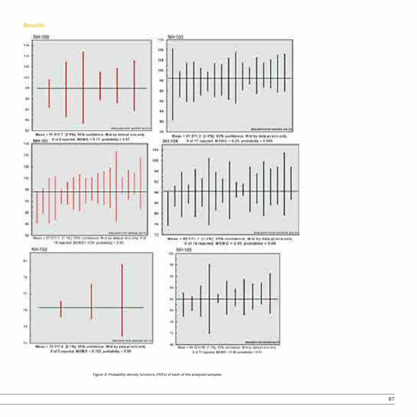
67

Results

Figure 4: Probability density functions (PDFs) of each of the analyzed samples.

68

Significant Age Peaks

Table 3: Displays differences in significant age peaks by each member, and from each transect.

Statistical Analysis Samples were compared statistically using a variety of tests. The “overlap” test measures the degree to which the age population of one sample matches with the age population of another sample: a value of 0 indicates no overlap, and a value of 1.0 indicates perfect overlap. The “similarity” test measures the degree of similarity between the overlapping ages: a value of 0 indicates no similarity, and a value of 1.0 indicates perfect similarity. Combined, these tests measure whether the relative abundances of various age populations are comparable.

Results of the overlap and similarity tests are tabulated in Tables 4 & 5. The Baker Canyon member, despite having the highest value in overlap, has a moderate value of 0.577 with a moderate-high value in similarity with a 0.768. The Schulz Ranch member had an extremely low value in overlap with a 0.126, but the highest value in similarity with a 0.825. The Pleasants Sandstone member had a low value of 0.339 in overlap, and a high value of 0.804 in similarity. These results were surprising, considering they were collected from the same members.

Another surprising aspect shown in the data was the consistently moderate-high value of both overlap and similarity between the northern Baker Canyon (NH-100) and the southern Pleasants (NH- 105) members.

Member Significant Detrital Zircon Age Peaks

Pleasants Sandstone

75 + 1 Ma (north only) 84 + 1 Ma (north only) 92 + 2 Ma (north only) Continuous 83-105 Ma (south only)

Schulz Ranch Sandstone 104 + 4 Ma

Baker Canyon Conglomerate 105 + 5 Ma 117 + 2 Ma (south only)

Figure 5: A depiction of the overlap and similarity tests. Sample A yields an identical population den-sity function (pdf) to the reference pdf, indicating that is has perfect overlap and similarity. Sample B has perfect overlap, shown by identical age peaks, but the similarity to the reference pdf is not perfect; it does not have the same population of zircons at each peak that

Figure 6: A probability Density Function (PDF) showing all samples. X-axis is modified to show only 50-200 Ma.

the reference sample does. Sample C has low overlap to the reference pdf because its age peaks are not the same as those of the reference curve. Sample C also has low similarity, indicating that the peaks that are located in overlapping loca-tions to the reference pdf do not have similar populations at those peaks. Figure after Gehrels (2000).

showing all samples. X-axis is modified to show

Overlap NH-100 NH-103 0.577 NH-103 NH-101 0.318 0.531 NH-101 NH-104 0.357 0.294 0.126 NH-104 NH-102 0.409 0.554 0.379 0.225 NH-102 NH-105 0.767 0.537 0.404 0.391 0.339

NH-101

Similarity NH-100 NH-103 0.768 NH-103 NH-101 0.747 0.756 NH-101 NH-104 0.702 0.788 0.825 NH-104 NH-102 0.388 0.479 0.526 0.753 NH-102 NH-105 0.700 0.733 0.789 0.898 0.804

NH-100 NH-103 NH-101 NH-104 NH-102 NH-105 NH-100 0.007 0.000 0.000 0.000 0.000 NH-103 0.007 0.000 0.000 0.000 0.000 NH-101 0.000 0.000 0.019 0.000 0.001 NH-104 0.000 0.000 0.019 0.000 0.879 NH-102 0.000 0.000 0.000 0.000 0.000 NH-105 0.000 0.000 0.001 0.879 0.000

Table 4 shows the overlap of samples. Boxes in bold are those of the same member from the northern and

southern transects.

Table 5 shows the similarity of each sample. Boxes in bold are those of the same member from the northern

and southern transects.

Table 6: K-S test between samples. Statistically significant values great than 0.05 are highlighted.

69

A third statistical test used to compare detrital zircon samples is the Kolmogorov-Smirnoff (K-S) test: a mathematical computation to determine if there is a statistically significant difference between two detrital zircon populations. This can be used to determine the likelihood that the detrital zircon populations were derived from the same source. A K-S p-value greater than 0.05 gives a 95% confidence that the two samples are not statistically different. In other words, we are looking for a value greater than 0.05, which will indicate to us that a pair of samples are statistically similar.

Table 6 shows the K-S test of samples; values that are not highlighted are rejected for being too significantly different from the compared dataset. NH-104 and NH-105, the Schulz and Pleasants Members, respectively, are the only two samples that can be noted as being statistically significant, despite not being from the same member.

A cumulative distribution function (CDF) depicts the percentage of detrital zircon grains with ages less than noted on the axis. This is another way to visualize the similarities and differences between samples. NH-100, the northern sample of the Baker Canyon Conglomerate has a much larger proportion of pre-Mesozoic zircons.

InterpretationsMaximum Depositional Ages of Zircons

Table 7: Displays the stratigraphic age that corresponds with the maximum depositional ages from each sample in the north and the south.

Table 7 displays the stratigraphic age (Cooper, 1986) with the maximum depositional ages from both the northern and southern transects. Since there is such a large difference between the stratigraphic ages and the maximum depositional ages, possibilities for the anomalies are as follows: Assuming the stratigraphic ages are correct, the Baker Canyon Member presents us with concordant maximum depositional ages, though there is a gap between the stratigraphic age. A reason for this is the absence of modern zircons, which could be due to magmatism being underground, and therefore not exposed to be eroded into the basin. Another possibility is that if eruptions were occurring at this time of deposition, they may not have been local. If so, these eruptions may not have been pyroclastic, spewing zircons into the air, and wind direction may not have been favorable to the western side of the arc. The Schulz Ranch, same as the Baker Canyon, exhibits this gap between the maximum depositional ages and the reasons for this may be the same as mentioned, but it also exhibits another element of change. The maximum depositional ages, though they exhibit only a small gap, show a difference in age. The reason for this could be that the drainage basin may not be well mixed, or may be completely separate drainage basins being fed by separate sources. The Pleasants Sandstone intensifies this gap exclusive to the southern sample, as the northern sample has an introduction of modern zircons, resulting in an age that fits into the stratigraphic age constraints.

The majority of the detrital zircons from each sample are arc derived and the age distribution of pre-arc zircons match those present in the metamorphic framework (Figure 8). This northern Baker Canyon sample had the largest number of pre-Mesozoic zircons, so it was selected to compare age peaks to a combined sample of Peninsular Ranges wallrock data. The shaded region indicate the main locations of overlap.

Figure 8: Stacked PDF comparing ages of detrital zircons from the Baker Canyon Member and a combined sample of northern Peninsular Ranges wallrock (personal communication with Dr. Marty Grove for wallrock data).

Formation Member Stratigraphic Age Sample Number Maximum Depositional Age

Williams Formation

Pleasants Sandstone

83 Ma to 70 Ma

NH-102 (North) 75.3 + 1.8 Ma NH-105 (South) 84.0 + 1.2 Ma

Schulz Ranch Sandstone

NH-101 (North) 97.3 + 1.4 Ma NH-104 (South) 88.5 + 1.4 Ma

Ladd Formation

Holz Shale 89 Ma to 83 Ma Not sampled Baker Canyon Conglomerate

91 Ma to 89 Ma NH-100 (North) 97.9 + 3.0 Ma NH-103 (South) 97.0 + 1.6 Ma

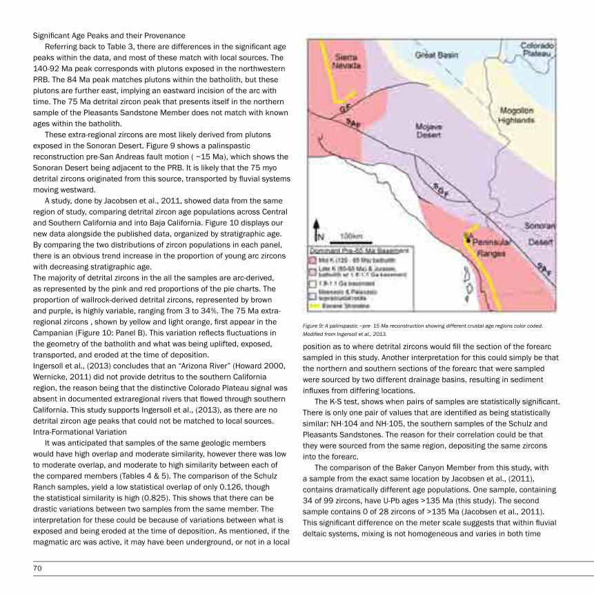
70

Significant Age Peaks and their ProvenanceReferring back to Table 3, there are differences in the significant age

peaks within the data, and most of these match with local sources. The 140-92 Ma peak corresponds with plutons exposed in the northwestern PRB. The 84 Ma peak matches plutons within the batholith, but these plutons are further east, implying an eastward incision of the arc with time. The 75 Ma detrital zircon peak that presents itself in the northern sample of the Pleasants Sandstone Member does not match with known ages within the batholith.

These extra-regional zircons are most likely derived from plutons exposed in the Sonoran Desert. Figure 9 shows a palinspastic reconstruction pre-San Andreas fault motion ( ~15 Ma), which shows the Sonoran Desert being adjacent to the PRB. It is likely that the 75 myo detrital zircons originated from this source, transported by fluvial systems moving westward.

A study, done by Jacobsen et al., 2011, showed data from the same region of study, comparing detrital zircon age populations across Central and Southern California and into Baja California. Figure 10 displays our new data alongside the published data, organized by stratigraphic age. By comparing the two distributions of zircon populations in each panel, there is an obvious trend increase in the proportion of young arc zircons with decreasing stratigraphic age.The majority of detrital zircons in the all the samples are arc-derived, as represented by the pink and red proportions of the pie charts. The proportion of wallrock-derived detrital zircons, represented by brown and purple, is highly variable, ranging from 3 to 34%. The 75 Ma extra-regional zircons , shown by yellow and light orange, first appear in the Campanian (Figure 10: Panel B). This variation reflects fluctuations in the geometry of the batholith and what was being uplifted, exposed, transported, and eroded at the time of deposition.Ingersoll et al., (2013) concludes that an “Arizona River” (Howard 2000, Wernicke, 2011) did not provide detritus to the southern California region, the reason being that the distinctive Colorado Plateau signal was absent in documented extraregional rivers that flowed through southern California. This study supports Ingersoll et al., (2013), as there are no detrital zircon age peaks that could not be matched to local sources.Intra-Formational Variation

It was anticipated that samples of the same geologic members would have high overlap and moderate similarity, however there was low to moderate overlap, and moderate to high similarity between each of the compared members (Tables 4 & 5). The comparison of the Schulz Ranch samples, yield a low statistical overlap of only 0.126, though the statistical similarity is high (0.825). This shows that there can be drastic variations between two samples from the same member. The interpretation for these could be because of variations between what is exposed and being eroded at the time of deposition. As mentioned, if the magmatic arc was active, it may have been underground, or not in a local

position as to where detrital zircons would fill the section of the forearc sampled in this study. Another interpretation for this could simply be that the northern and southern sections of the forearc that were sampled were sourced by two different drainage basins, resulting in sediment influxes from differing locations. The K-S test, shows when pairs of samples are statistically significant. There is only one pair of values that are identified as being statistically similar: NH-104 and NH-105, the southern samples of the Schulz and Pleasants Sandstones. The reason for their correlation could be that they were sourced from the same region, depositing the same zircons into the forearc. The comparison of the Baker Canyon Member from this study, with a sample from the exact same location by Jacobsen et al., (2011), contains dramatically different age populations. One sample, containing 34 of 99 zircons, have U-Pb ages >135 Ma (this study). The second sample contains 0 of 28 zircons of >135 Ma (Jacobsen et al., 2011). This significant difference on the meter scale suggests that within fluvial deltaic systems, mixing is not homogeneous and varies in both time

Figure 9: A palinspastic ~pre- 15 Ma reconstruction showing different crustal age regions color coded. Modified from Ingersoll et al., 2013.

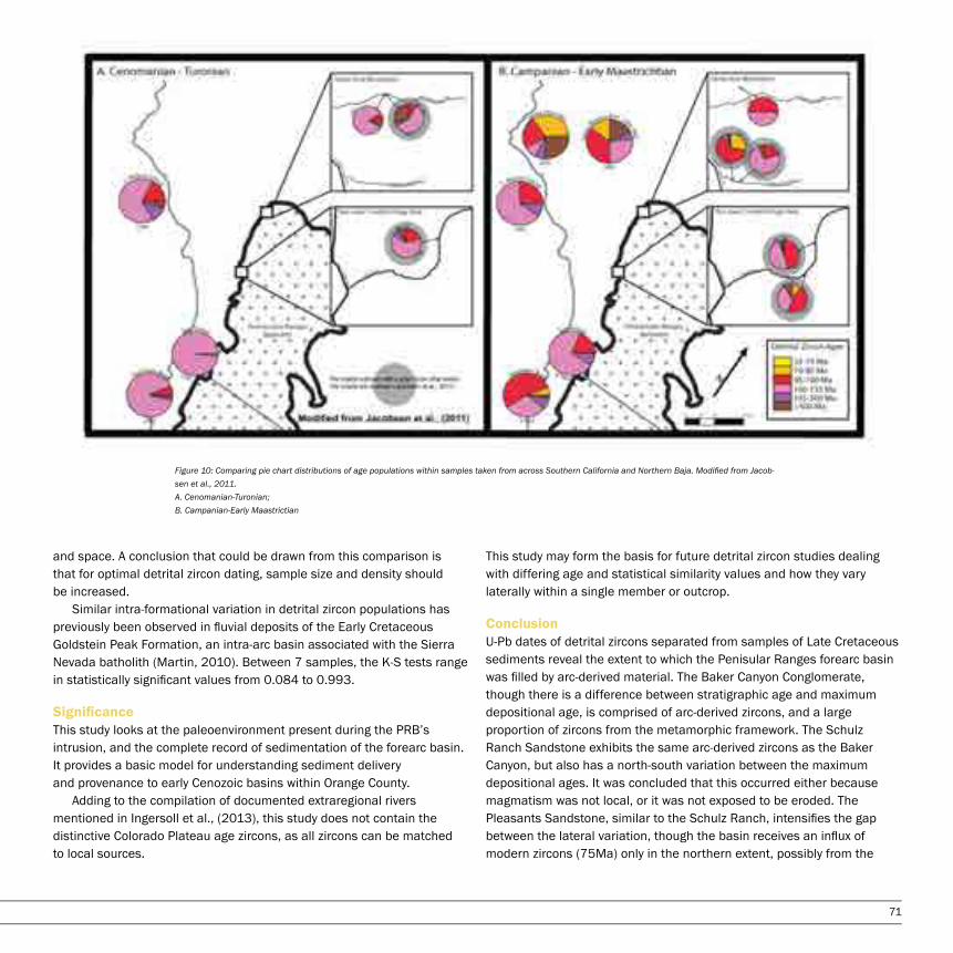
71

and space. A conclusion that could be drawn from this comparison is that for optimal detrital zircon dating, sample size and density should be increased.

Similar intra-formational variation in detrital zircon populations has previously been observed in fluvial deposits of the Early Cretaceous Goldstein Peak Formation, an intra-arc basin associated with the Sierra Nevada batholith (Martin, 2010). Between 7 samples, the K-S tests range in statistically significant values from 0.084 to 0.993.

SignificanceThis study looks at the paleoenvironment present during the PRB’s intrusion, and the complete record of sedimentation of the forearc basin. It provides a basic model for understanding sediment delivery and provenance to early Cenozoic basins within Orange County. Adding to the compilation of documented extraregional rivers mentioned in Ingersoll et al., (2013), this study does not contain the distinctive Colorado Plateau age zircons, as all zircons can be matched to local sources.

This study may form the basis for future detrital zircon studies dealing with differing age and statistical similarity values and how they vary laterally within a single member or outcrop.

ConclusionU-Pb dates of detrital zircons separated from samples of Late Cretaceous sediments reveal the extent to which the Penisular Ranges forearc basin was filled by arc-derived material. The Baker Canyon Conglomerate, though there is a difference between stratigraphic age and maximum depositional age, is comprised of arc-derived zircons, and a large proportion of zircons from the metamorphic framework. The Schulz Ranch Sandstone exhibits the same arc-derived zircons as the Baker Canyon, but also has a north-south variation between the maximum depositional ages. It was concluded that this occurred either because magmatism was not local, or it was not exposed to be eroded. The Pleasants Sandstone, similar to the Schulz Ranch, intensifies the gap between the lateral variation, though the basin receives an influx of modern zircons (75Ma) only in the northern extent, possibly from the

Figure 10: Comparing pie chart distributions of age populations within samples taken from across Southern California and Northern Baja. Modified from Jacob-sen et al., 2011. A. Cenomanian-Turonian; B. Campanian-Early Maastrictian

72

Sonoran Desert. Due to the variable nature of the northern and southern maximum depositional ages, it was concluded that mixing, within fluvial deltaic systems, is not homogeneous. Because of these surprising inter-formational variations, we recommend increased sample sizes and density for such depositional environments.

AcknowledgmentsThe project was funded by grant PRF#50146-UR8 from the American Chemical Society Petroleum Research Fund and California State University, Fullerton: Department of Geology.Special thanks to NSF Louis Stokes Alliance for Minority Participation grant NSF: HRD-0331537, and the staff of the Arizona Laserchron Center laserchron.org/laserchron

Thanks to Marty Grove (Stanford University), Ray Ingersoll (University of California, Los Angeles), and Carl Jacobsen (Iowa State University) for freely sharing their data and ideas about the Peninsular Ranges forearc basin.

ReferencesCooper, J.D. (1982). Late Cretaceous depositional environments and paleogeography, Santa Ana Mountains, Southern California. Los Angeles, Pacific Section, SEPM (Society for Sedimentary Geology), Field Trip Volume and Guidebook, 11-23.

Dickinson, W.R. (1995). Forearc Basins, in Busby, C.J., & Ingersoll, R.V., eds. Tectonics of Sedimentary Basins. Blackwell Science, Cambridge Massachusetts, 121-161.

Fritsche A.E., & Behl, R.J., eds. (2008). Geology of Orange County California and the Irvine Ranch National Natural Landmark. Long Beach, Pacific Section, SEPM (Society for Sedimentary Geology), 106, 52-142.

Gehrels, G.E. (2000). Introduction to detrital zircon studies of Paleozoic and Triassic strata in western Nevada and northern California, in Soreghan, M.J., & Gehrels, G.E., eds., Paleozoic and Triassic paleogeography and tectonics of western Nevada and northern California. Boulder, Colorado, Geological Society of America Special Paper 347, 1-17.

Howard, J.L. (2000). Provenance of quartzite clasts in the Eocene-Oligocene Sespe Formation: Paleogeographic implications for southern California and the ancestral Colorado River. Geological Society of America Bulletin 112-11, 1635-1649.

Ingersoll, R.V., Grove, M., Jacobsen, C.E., Kimbrough, D.L., & Hoyt, J.F. (2013). Detrital zircons indicate no drainage link between southern California rivers and the Colorado Plateau from mid-Cretaceous through Pliocene. Geology( in press). Article ID: G33807

Jacobsen, C.E., Grove, M., Pedrick, J.N., Barth, A.P., Marsaglia, K.M., Gehrels, G.E., & Nourse, J.A. (2011). Late Cretaceous-early Cenozoic tectonic evolution of the southern California margin inferred from provenance of trench and forearc sediments. Geological Society of America Bulletin v. 123, 485-506.

Martin, M.W. (2011). A detrital zircon provenance analysis of the Goldstein Peak Formation. M.S. Thesis, California State University, Fullerton 107, 20-63.

Wernicke, B. (2011). The California River and its role in carving Grand Canyon. Geological Society of America Bulletin v. 123, 1288-1316.

73

Metasomatism of the Bird Spring Formation near Slaughterhouse Springs, California


Taylor KennedyAdvisor: Brandon Browne

IntroductionUnderstanding how ore deposits develop is vital to our ability to locate and develop mineral resources. In particular, ore deposits containing precious metals like gold, copper, and lead, play a major role in our economy. In this study, I propose to characterize the ore mineralization of metasomatized Pennsylvanian Bird Spring Formation (Pbs) where in contact with the (1) high angle Slaughterhouse Fault and (2) Mid Hills quartz monzonite of the Cretaceous Teutonia batholith in the New York Mountains near Slaughterhouse Springs, California. Comparing the mineralization the Bird Springs Formation as a result of faulting-induced metasomatism and contact metamorphism will yield valuable insight into our understanding of how metasomatic ore deposits are related to contrasting geological phenomena.

Geologic HistoryThe geologic history of this region is best summarized by Burchfiel and Davis (1997), and Miller and Wooden (1993), and their results will be summarized here. The underlying bedrock of the New York Mountains is Precambrian gneiss (Pcgn). This unit consists of both meta-igneous and metasedimentary rocks with potassium feldspar augens. Unconform-ably overlying gneiss is the Cambrian Tapeats Sandstone (Ct), which is overlain by the Cambrian Bright Angel Shale (Cba), which is interbedded with calc-silicate and pelitic hornfels due to localized metamorphism. The Cambrian Bonanza King Formation (Cbz) unconformable overlies the Bright Angel Shale, and is subdivided into the lower Papoose Lake member (Cbl) and the Banded Mountain member (Cbu). The lower Pa-poose Lake is interbedded with calcite and dolomite that has locally been metamorphosed to marble. Overlying the Bonanza King is the Cambrian Nopah Formation (Cn), which is a coarse-grained white dolomite unit underlain by shale known as the Dunderberg Shale Member (Cd). Atop the Nopah Formation is the Devonian Sultan Limestone (Ds), which contains a lower member that is interbedded calcite and dolomite marble believed to be the metamorphosed equivalent of the Valentine Member (Dsv) found in other areas (Burchfiel and David 1997). It has an upper member called Crystal Pass (Dscp), which is a white limestone that has been metamorphosed to coarse grained marble. Lying nicely on top of Crystal Pass is the Monte Cristo Limestone (Mm). It has three members, from lower to upper: Dawn (Mmd), Anchor (Mma), and Buillion (Mmb).

The Dawn and Anchor members have been recrystallized into marble, but the Anchor contains chert nodules. Buillion is calcite and marble with very few chert nodules. The Bird Spring Formation overlies the Monte Cristo Limestone. Bird Spring is limestone and dolomite, and has been metamorphosed to low grade marble in many places. Its exact date of deposition is unknown but it is restricted to the upper Mississippian to Pennsylvanian and possibly the Permian. Unconformable overlaying the Bird Spring is a calc-sillicate rock (Mcs). This unit has been proposed to have been deposited during the Mesozoic, as well as the next unit in the sequence: volcanic and sedimentary rocks (Mmvs). Atop of these unknown units we have the Mesozoic Sedimentary Rocks of Sagamore Canyon. This unit correlates with the nonmarine environment of the south-eastern California region and places us back on track with a time scale. Things finally get exciting with an intrusion of magma that has been the cause of some of the metamorphism in the area. This magma is now coarse grained quartz monzonite to monzonite with phenocrysts of potassium feldspar (Mp). Things continue to be exciting since the Slaugh-terhouse Fault ripped across the area. It is also responsible for the rest of the metamorphism of the units. Following this faulting is the Tertiary volcanic rocks (Tv). This is a unit of volcanic breccias that is associated with a late Miocene-Pliocene volcanic event (Burchfiel and Davis 1997). The last unit to be deposited in the New York Mountains is alluvium units in the Quaternary; an older unit (Qoal) and a younger unit (Qal).

Proposed MethodologyI intend to hike around the Bird Spring formation mapping the contacts between rock units, the extent and style of the metamorphism and meta-somatism, and the geologic structures such a faults and folds. In addition to completing a ~1.5 km2 geological map of the area, I will focus on two sampling sights; one on the western flank of the Bird Spring Formation where it has been intruded by Cretaceous quartz monzonite and the other along the northern flank where the Bird Spring Formation is in con-tact with the Slaughterhouse fault. Samples will be described in terms of mineralogy and texture in order to give a better understanding of the ore development at these two contrasting sites.

74

TimelineFieldwork and sample collection August-September, 2012 Thin section preparation and production October-November, 2012 Thin section analysis via SEM December-January, 2013Interpretation of results February-March, 2013First Draft, Thesis April 26, 2013

ReferencesBurchfiel, B., & Davis, G. (1977). Geology of the Sagamore Canyon-Slaughterhouse Spring Area, New York Mountains, California. Geological Society of America Bulletin, 88(11), 1623-1640.

Miller, D., & Wooden, J. (1993). Geologic Map of the New York Mountains area, California and Nevada. U.S. Geological Survey. 93-198

U.S. Geological Survey, (1983). Ivanpah Quadrangle California-San Ber-nardino Co. 7.5 Minute Series (Topographic).

Map of my field area. I will be mapping the two square miles between (656, 3908) and (658, 3909). Provided by USGS 1983

75

Robust Statistical Modeling of Neuronal Intensity Rates

Department of Mathematics, College of Natural Sciences and Mathematics, California State University, Fullerton, CA, USA

Jenny C. ChangAdvisor: Dr. Sam Behseta

AbstractIn our research, we develop a statistical hypothesis-testing paradigm based on a nonparametric resampling technique to compare neuronal firing intensity functions obtained from a scientific study of the primary motor cortex, subjected under two experimental conditions (Matsuzaka et. al, 2007). Our approach revolves around resampling neuronal spike trains as an aggregate of time points, or point processes, preserving the spiking nature of each trial recorded during the experimented task. In this context, the null hypothesis reflecting no statistical differences between the neuronal firing rate curves, fitted to the spiking activities of a single motor neuron under the two conditions, is tested nonparametrically. We hypothesize that both sampling with and without replacement will yield the same statistical hypothesis test. Our results show that either of the approaches can be used to detect the nuances between the spiking patterns of the two conditions. The statistical detection of differences between the firing patterns of M1 neurons gives way to further investigation associated with the role of M1 in executing and planning fully-learned movements.

IntroductionFor centuries, the dominating theory in neuroscience suggested that the brain was an immutable organ, incapable of generating new neuronal connections even after prolonged exposure to changes in environment or acquisition of new knowledge. However, in recent years, the scientific community has witnessed the emergence of the theory of neuroplasticity, in which the brain is deemed capable of developing distinct neuronal pathways that were not present during the initial formation of the neural network. This change in thought prompted further scientific studies to reexamine previous misconceptions involving the correlation between activities in certain regions of the brain with specific functions carried out by the body. More specifically, an interest lies in examining the effects of plasticity on the primary motor cortex (M1) area of the brain. Prior notions associated M1 with simple motor usage and execution of motor movements but disregarded its connection to the planning or storing of movements, which was generally attributed to originating from the prefrontal cortex (Campbell 1905; Fulton 1935; Jacobsen 1934). However, with the advent of technological tools such as intracortical electrical stimulation mapping and functional MRI’s,

neuroscientists are recognizing M1 as another storage site and learning center for motor movements (Karni et al. 1995, 1998; Sanes et al. 2000; Plautz et al. 2000).

Experimental BackgroundTo investigate the implications of neuroplasticity of the primary motor cortex, Matsuzaka et al. (2007) conducted a year-long scientific study on two Macaca Mulatta monkeys, during which the activity of the monkeys’ M1 neurons was recorded in correlation with their movements to hit one of five illuminated targets arranged horizontally on a touch-sensitive screen (Fig. 1). The monkeys were trained to react to the visual stimuli, which were presented as a row of digits numbered from one to five, under two experimental conditions: random mode and repeating mode. For the random mode, targets were displayed in a pseudorandom order to simulate M1’s response to an unlearned or semi-learned movement while the repeating mode displayed the targets as a sequence of repeating triplets to simulate M1’s response to a fully learned movement. A time period of 800-ms was given for the monkeys to react to the visual cue, during which the touch screen would either produce a 1-kHz tone upon the monkey’s contact with the correct target or produce a 50-Hz tone upon contact with an incorrect target. The firing activities of the M1 neurons were recorded in correspondence to the response time (RT) values of the monkeys’ reactions. The measure of RT values, defined as the time interval between successive target hits minus the delay, was an especially important tool in defining the characteristics of the repeating mode. As explained in the work, “Skill representation in the Primary Motor Cortex after long-term practice,” by Matsuzaka et al.:

“To promote the occurrence of predictive responses, defined as RT < 150 ms, we delayed the fill of the next target after a correct response by 400 ms. Monkeys were permitted to make responses during the 400-ms delay, leading to negative RT values. When the monkeys made a correct response during this delay, the target was not filled and the task was incremented to the next target in the sequence. Thus a fully trained animal could (and did) perform the correct sequence in the Repeating mode without visual cues to guide their movements” (Matsuzaka et al. 2007).

76

r1,i = { t1,i, t2,i,…, tki, i },

where ki is the number of firings (spikes) per trial i and t is the firing or spiking time. Therefore, r1,i defines a simple point process. Similarly, let

r2,i = { s1,i, s2,i, …, sji,i },

where ji is the number of spikes per trial i and s is the firing time. For a given neuron, we define:

RasterW={r1,u };u= 1,…,n1

andRasterO={r2,u }; u= 1,…,n2

for the with replacement and without replacement methods, respectively. As seen in Figure 2, the top half of the graph displays a raster plot

illustrating individual tick marks, which represent a single neuronal firing occurring in one millisecond (ms), structured in rows corresponding to a single trial, where each trial is defined as the completion of one block of the experiment. By utilizing the Peri-Stimulus Time Histogram tool, we create a summary of the neuronal activity by employing histograms that reflect the firing patterns of a neuron against time, presented in the bottom half of Figure 2. For each histogram, there is a time period of 200-ms before the monkey touched the lighted target up until the 100-ms that occurred after the contact. To create the PSTH for each neuron, we first segmented the time period into a series of 10-ms bins. Then, we counted the total number of spikes that fell within each 10-ms time interval and pooled the spike occurrences across all trials. By dividing the spike counts per bin by the total number of trials, we obtain an adjusted histogram where each bar of the histogram represents the rate of spikes per trial.

The raster plots and PSTH are helpful as an initial summarizing

Figure 1. A monkey reaches for the touch-sensitive screen displaying targets numbered from 1- 5, which may be illuminated in a random or repeating mode (Image source: Matsuzaka et al. 2007).

Research ObjectivesThe main inquiry of this work is to determine differences between the random mode and the repeating mode on a global and local level. A global analysis will help scientists determine whether a neuron should be considered for further study, while the local analysis will help determine the significance of the neurons at specific time bins. To address the problem of comparing the neuronal firing rates, we devise two resampling tests: with and without replacement. We hypothesize that both proposed approaches will yield the same statistical hypothesis test, either of which can be used to detect the nuances between the spiking patterns of the two conditions. This method is different from the usual sampling technique of bootstrapping, which is solely built around the idea of “without replacement” (Efron 1982). Our objective is to show that the two resampling approaches yield the same type of inferential answer, and whether the resampling is done with or without replacement, we will arrive at the same scientific conclusion. This approach is mainly useful because when firing patterns of M1 neurons are found to be statistically differential, one may conclude that the role of M1 in the planning and execution of fully-learned movements, as opposed to semi-learned or unlearned movements, is significant. Additionally, our method serves the purpose of screening out those neurons that remain nonresponsive to the experimental objectives (Behseta et al 2005).

MethodsSummarizing Spike TrainsIn the study conducted by Matsuzaka et. al (2007), microelectrodes were inserted in the M1 area of the monkeys’ brains to gather the neuronal spiking data that we analyze. We collected neuronal spiking data for twenty neurons in both the random and repeating mode. In order to organize the large collection of data, we summarize the neuronal spikes by utilizing raster plots and Peri-Stimulus Time Histograms (PSTH) to denote the firing activity for each trial (Fig 2). Let n1 and n2 be the total number of trials in the random and repeating mode, respectively. For the ith trial in the random mode, suppose Figure 2. Raster and PSTH plots for a neuron under repeating (left panel) and random (right panel) modes.

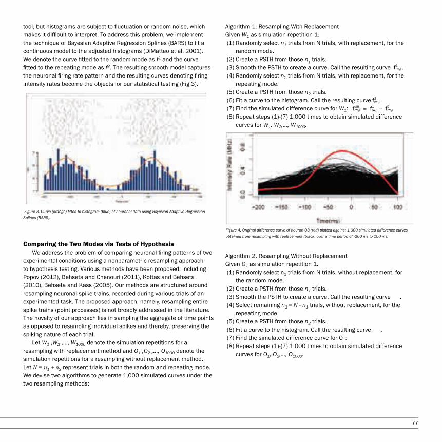
77

tool, but histograms are subject to fluctuation or random noise, which makes it difficult to interpret. To address this problem, we implement the technique of Bayesian Adaptive Regression Splines (BARS) to fit a continuous model to the adjusted histograms (DiMatteo et al. 2001). We denote the curve fitted to the random mode as f1 and the curve fitted to the repeating mode as f2. The resulting smooth model captures the neuronal firing rate pattern and the resulting curves denoting firing intensity rates become the objects for our statistical testing (Fig 3).

Figure 3. Curve (orange) fitted to histogram (blue) of neuronal data using Bayesian Adaptive Regression Splines (BARS).

Comparing the Two Modes via Tests of Hypothesis We address the problem of comparing neuronal firing patterns of two

experimental conditions using a nonparametric resampling approach to hypothesis testing. Various methods have been proposed, including Popov (2012), Behseta and Chenouri (2011), Kottas and Behseta (2010), Behseta and Kass (2005). Our methods are structured around resampling neuronal spike trains, recorded during various trials of an experimented task. The proposed approach, namely, resampling entire spike trains (point processes) is not broadly addressed in the literature. The novelty of our approach lies in sampling the aggregate of time points as opposed to resampling individual spikes and thereby, preserving the spiking nature of each trial.

Let W1 ,W2 ,…, W1000 denote the simulation repetitions for a resampling with replacement method and O1 ,O2 ,…, O1000 denote the simulation repetitions for a resampling without replacement method. Let N = n1 + n2 represent trials in both the random and repeating mode. We devise two algorithms to generate 1,000 simulated curves under the two resampling methods:

Algorithm 1. Resampling With ReplacementGiven W1 as simulation repetition 1. (1) Randomly select n1 trials from N trials, with replacement, for the random mode. (2) Create a PSTH from those n1 trials. (3) Smooth the PSTH to create a curve. Call the resulting curve . (4) Randomly select n2 trials from N trials, with replacement, for the repeating mode. (5) Create a PSTH from those n2 trials. (6) Fit a curve to the histogram. Call the resulting curve . (7) Find the simulated difference curve for W1: (8) Repeat steps (1)-(7) 1,000 times to obtain simulated difference curves for W1, W2,…, W1000.

Algorithm 2. Resampling Without ReplacementGiven O1 as simulation repetition 1. (1) Randomly select n1 trials from N trials, without replacement, for the random mode. (2) Create a PSTH from those n1 trials. (3) Smooth the PSTH to create a curve. Call the resulting curve . (4) Select remaining n2 = N - n1 trials, without replacement, for the repeating mode. (5) Create a PSTH from those n2 trials. (6) Fit a curve to the histogram. Call the resulting curve . (7) Find the simulated difference curve for O1: (8) Repeat steps (1)-(7) 1,000 times to obtain simulated difference curves for O1, O2,…, O1000.

f1(W1)

f2(W1)

f1(W1)fdiff

(W1) f2(W1)= −

Figure 4. Original difference curve of neuron O3 (red) plotted against 1,000 simulated difference curves obtained from resampling with replacement (black) over a time period of -200 ms to 100 ms.

78

ResultsThe fundamental questions that scientists hope to answer by comparing the firing patterns are, first, to see how the curves compare on a global level over an entire period of time and, second, to detect how the curves compare on a local level over snippets of time. Global Analysis

To determine how the curves compare globally or universally, we recast that question in terms of hypothesis testing. We formulate and test the null hypothesis H0, where

H0: f1 − f2 = 0represents the statistical differences between the fitted curves of the two testing conditions. More specifically, if we find that the difference curve obtained from subtracting the curves fitted to the random and repeated data sets is flat, then we have no reason to believe that the random mode differs from the repeating mode. In Figure 6, we highlight the graphical representations of six neurons that demonstrate the most dominant modes of variations among the twenty-five neurons we examined. We are interested in determining how the original difference curve compares with the 1,000 simulated curves for each neuron. We analyze the difference curves obtained from point-wise subtraction of the random and repeating mode (denoted in red) as well as their simulations (denoted in black). In the case where the original difference curve extends to regions far more extreme (α < 0.01) than the simulation curves, we classify the difference between the two modes as statistically significant. Similarly, if the simulation curves are extreme, one can conclude that there is no sufficient statistical support to indicate significant differences between the two modes. We also examine the general shape of the original difference curve and simulation curves for the two hypothesis testing approaches, namely, with replacement

and without replacement. We conclude that, although we utilized two different resampling methods, there is a consistency in the relationship between the firing pattern of the original difference curve as well as the one associated with simulation curves. Below, we document these findings with the aid of graphical and numerical summaries. Local Analysis For the local analysis of the neuronal firing intensities, we compare the p-values of data for individual time bins. To interpret how the curves compare locally, we concentrate on subwindows of time. For both of the replacement methods, we calculate the p-values denoted by

Pw =

and

P0 =

where

foriginal = frandom − frepeating.

The p-value may be viewed as an expected value E(x) of a sequence of n 1’s and 0’s, equally weighted . In other words, let

In(A) = {and

Im(B) ={

define the indicator functions for with and without replacement, respectively. Thus, we have

Pvalue.with = lim E(In(A))

and

Pvalue.without = lim E(Im(B)).

Our empirical results suggest that

Pvalue.with ≈ Pvalue.without.

The p-values included in Table 1 are consistent with the graphical representations shown in Figure 4 and 5 for Neuron O3. On both occasions,

Figure 5. Original difference curve of neuron O3 (red) plotted against 1,000 simulated difference curves obtained from resampling without replacement (black) over a time period of -200 ms to 100 ms.

#Wi > foriginal

#Oi > foriginal

1000

1000

n→∞

m→∞

1, A:Wi > foriginal

0, Ac

1, B:Oi > foriginal

0, Bc

1n

79

Table 1. Comparison of difference curves for Neuron O3 obtained by random sampling with replacement (blue) and without replacement (green). The P-values falling under 0.01 are denoted in red.

Figure 6. Graphical representations of six neurons whose difference curves, denoted in red, is compared to 1,000 simulated curves, denoted in black, under two resampling methods: with replacement and withoutreplacement. Each neuron is represented with a block of two figures, where the top panel displays the values obtained using with replacement and the lower panel displays the values obtained using without replacement approach to hypothesis testing. In each block, firing intensity rates have the same fluctuations regardless of the testing approach. Also, statistical significance can be detected with either of the approaches, as they provide similar confidence interval coverage.

80

we have strongly significant differences at a window ranging from -100-ms to 50-ms. This could be interpreted as a sign that, for this neuron, the two modes were manifested in highly differential firing patterns at the vicinity of the screen touch, whereas the two modes resulted in similar patterns at the anticipation window prior to the screen touch. To summarize, we have shown that the global and local results aid in the scientists’ analysis of the M1 neurons. For the global analysis, the scientists can rule out certain neurons that are not conducive to the experimental objective by screening out those that have flattened original and simulated difference curves. The local analysis assists in determining the significance of neurons at specific time points over the experimental time interval by pinpointing differential patterns within subwindows of time. We can conclude that the two resampling approaches, with replacement and without replacement, create the same type of inferential answer. Statistical significance can be detected with either of the resampling approaches, as they provide similar confidence interval coverage.

DiscussionThe results we obtained through resampling neuronal spike trains using with and without replacement are interesting contributions to both the statistical and neuroscientist communities. Statisticians generally rely on the usual method of bootstrapping (with replacement) when conducting resampling tests. Our results show that, as long as we choose a large number of simulations, both with and without replacement methods are viable approaches in the context of resampling neuronal spike trains. In addition, our method of resampling point processes, instead of individual spikes, is not broadly addressed in statistical literature. Our results contribute to the neuroscientists because we are able to provide a method for them to filter out neurons through the global analysis and determine significance at specific time intervals through the local analysis. Our results strengthen our recommendation to offer both resampling methods to the neuroscientists and assure that utilizing either method will generate the same scientific conclusion. Furthermore, our method of sampling neurons as an aggregate of time points, as opposed to individual time points, helps the scientists remain computationally cost-efficient. In addition, our result strips away any limitations to the methods of hypothesis testing that may have been present when determining which computational methods are most effective for analyzing the neuronal firing patterns of the neurons in the primary motor cortex.

One of the limitations to our method is that due to the asymptotic nature of the underlying theoretical results, a large number of simulations must be performed in order for the methods to produce the same scientific conclusion. In the case of our work, we chose to have 1,000 simulations to be used during resampling. Another limitation to our method is that our analysis was limited to simulation-based approaches.

We did not fully delve into the theoretical side of the resampling process; however, we plan to study the theoretical aspects of this methodology. For future studies, we propose the same type of resampling simulation-based analysis to build a classification method. Utilizing principal component analysis, we hope to find the most dominating modes of differences between the random mode and repeating mode. By identifying those modes, we can categorize neurons by their class of differences. A further application of our method would be to investigate the computational complexity we are introducing to the methodology as the number of experimental conditions grows. Moreover, we would like to establish how computationally cost-efficient our methodology would be if we increase the number of time bins, data points, and experimental conditions. We would like to see how the computational costs of utilizing our method would change if we varied the size of the simulation. We would determine whether or not the implementation of our method would result in any cost and energy savings that would be significant enough to prompt a transition from previous computational methods to our method.

AcknowledgementsI would like to thank Dr. Behseta for challenging me to continually push beyond my limits. I am grateful for his never-ending support and guidance throughout this entire journey. I would also like to thank the CSUF McNair Scholars Program for providing the resources necessary for a successful research experience.

ReferencesBehseta, S., Chenouri, S. (2011). Comparison of Two Population of Curves with an Application in Neuronal Data Analysis. Statistics in Medicine (30): 1441–1454.

Behseta, S. and Kass, R.E. (2005). Testing Equality of Two Functions using BARS. Statistics in Medicine (24): 3523-34.

Behseta, S., Kass, R.E., and Wallstrom, G.L. (2005). Hierarchical models for assessing variability among functions. Biometrika (92): 419-434.

Campbell, A. W. (1905). Histological Studies on the Localization of Cerebral Function.Cambridge, UK: Cambridge Univ. Press.

DiMatteo, I., Genovese, C.R. & Kass, R.E. (2001). Bayesian curve-fitting with free-knot splines. Biometrika (88): 1055-73.

Efron, B. (1982). The jackknife, the bootstrap and other resampling plans. Montplier, VT: Capital City Press.

Fulton JF. (1935). Definition of the “motor” and “premotor” areas. Brain

81

(58): 311– 316.

Jacobsen, C.F. (1934). Influence of motor and premotor lesions upon retention of acquired skilled movements in monkey and chimpanzees. Assoc Res Nerv Ment Dis (13): 225–247.Karni, A., Meyer, G., Jezzard, P., Adams, M.M., Turner, R., Ungerleider, L.G. (1995). Functional MRI evidence for adult motor cortex plasticity during motor skill learning. Nature (377): 155–158.

Karni, A., Meyer, G., Rey-Hipolito, C., Jezzard, P., Adams, M.M., Turner, R., & Ungerleider, L.G. (1998). The acquisition of skilled motor performance: Fast and slow experience-driven changes in primary motor cortex. Proceedings of the National Academy of Science USA (95): 861–868.

Kottas, A., and Behseta, S. (2010). Bayesian Nonparametric Modeling for Comparison of Single-Neuron Firing Intensities. Biometrics (66): 277-286.

Matsuzaka, Y., Picard N. & Strick, P. L. (2007). Skill representation in the Primary Motor Cortex after long-term practice. Journal of Neurophysiology (97): 1819-1832.

Plautz, E.J., Milliken, G.W., Nudo, R.J. (2000). Effects of repetitive motor training on movement representations in adult squirrel monkeys: role of use versus learning. Neurobiol Learn Mem (74): 27–55.

Popov, M.Y. (2012). Assessing Uncertainty of Clustered Neuronal Intensity Curves. Dimensions (14): 45-53.

Sanes, J. & Donoghue, J. (2000). Plasticity and primary motor cortex. Annual Review of Neuroscience (23): 393-415.

82

Inequalities Obtained from the Isoperimetric Inequality for Planar Curves


Asha CyrsAdvisor: Bogdan D. Suceava

1. Introduction: The Many Forms of Isoperimetric InequalityThe importance of the Isoperimetric Inequality is described in Chapter

5 from Frank Morgan's monograph Geometric Measure Theory [8]. Isaac Chavel's infuential monograph [1] is dedicated entirely to the topic of isoperimetric inequalities and covers many extensions and developments in various geometric contexts. There is a large literature developed on this important class of mathematical problems, from classical surveys e.g. [5] to recent research contributions, e.g. [2]. In the present note we will explore only the context of isoperimetric inequality in planar domains bounded by closed simple planar curves. This discussion is related to section 1.15 in George Pólya and Gabor Szegö's Isoperimetric Inequalities in Mathematical Physics, where the case of plane domains is discussed. Our goal in this note is to explore and illustrate the isoperimetric inequality in planar domains through several examples. In the CSUF curriculum, the Isoperimetric Inequality is studied in the following context (see [6], p.58 et al.) Let γ be a simple closed curve in the plane, let L be its length and let A be the area contained by it. Then 4A ≤ L2,

and the equality holds if and only if γ is a circle. The proof in A. Pressley's textbook relies on Wirtinger's Inequality, which states the following (see [6], p. 59). Let F : [0,] → R be a smooth function such that F(0) = F() = 0. Then

and the equality holds if and only if F(t) = D sin t, for all t ∈ [0, ], where D is a constant. We should point out that the elementary form of Isoperimetric Inequality is also encountered in the undergraduate curriculum in an al-gebraic context: the so-called Brunn-Minkowski's inequality. This classical problem was assigned a decade ago as a Putnam competition problem; it was also a problem proposed in the Irish Olympiad in 1992.

Problem (W. L. Putnam Competition, 2003.) Let a1, a2,...,an, b1, b2,..., bn ≥ 0, n ≥ 1. Prove that:

Solution: Suppose in the first case that there is an index j ∈ {1,...,n} suchthat aj + bj = 0. Then the inequality is 0 ≤ 0. Suppose in a second case that there exists j ∈ {1,...,n} such that aj = 0, but bj ≠ 0. Then the inequality is:

which is true. Finally, suppose that: for any j ∈ {1,...,n}, aj ≠ 0, bj ≠ 0. The we can apply AM-GM inequality as follows:

The equality holds if and only if: However, what is the connection between this Problem and the isoperimetric inequality for planar curves, presented at the beginning of this section? The algebraic inequality asked in the Putnam competition first appears at the end of 19th century in [7]. The Brunn-Minkowski inequality is presented in the infuential monograph [3], p.277, where it serves to prove a more general version of the isoperimetric inequality. That's why we can say that both the inequality 4A ≤ L2 and Brunn-Minkowski inequality are both different facets of the same phenomenon. In the well-known monograph [4] there are several sections dedicated to various forms of the Brunn-Minkowski inequality. On the websitehttp://www.unl.edu/amc/a-activities/a7-problems/putnamindex.shtmlthere are three other solutions presented to this Putnam problem.Therefore, there are many forms that the isoperimetric inequalities could

83

take and there is a large diversity of mathematical tools one can use to approach this class of problems.

2. Length and Area: Brief Reminder from CalculusIn our calculus courses, we learn that ([9], p.492) if a curve γ is described by the parametric equations x = f(t), y = g(t), α ≤ t ≤ β, where f and g are differentiable functions with continuous derivative on [α,β] and γ is traversed exactly once as t increases from α to β, then the length of γ is

If the curve is written in polar coordinates, then r = f(θ); a ≤ θ ≤ b, and we regard the polar angle θ as a parameter. Assuming that the derivative of the function f is continuous, then the length of γ is ([9], p. 507):

The area of the region enclosed by γ is ([9], p. 505):

We will be using these formulas later in this note.

3. A Classical ProblemIn [6], Problem 3.2.2 asks the following. By applying the isoperimetric inequality to the ellipse

where p and q are positive constants, prove that

The equality holds if and only if p = q. The solution suggested in [6] is straightforward. Parametrizing the ellipse by γ(t) = (p cos t, q sin t), for 0 ≤ t ≤ 2, its area can be computed directly by a consequence of Green's formula: A = pq. The left hand side term in the inequality we need to show represents the perimeter of the ellipse. Hence, the isoperimetric inequality 4A ≤ L2 is

Thus, we can say that this inequality was derived from applying the isoperimetric inequality to a certain planar curve. In this context it is natural to ask: what other inequalities can be obtained by applying the isoperimetric inequality to other planar curves? Also, what geometric interpretations we can obtain from these inequalities?

4. ExplorationPursuing the idea presented in the previous section, we will explore

what other inequalities are derived by applying the isoperimetric inequality to other plane curves, instead of the ellipse, as we have seen in Section 3. Our quest is for examples of planar curves other than the ellipse that generate similar inequalities when we substitute their area and their length into the isoperimetric inequality.

Example 4.1. One of the classical curves is the astroid, given by the parametric equations x = a cos3 t; y = a sin3 t. Its area is (see [9], problem 30/page 494) A = 3/8a2. Astroid's length is (see [9], problem 50/page 494) L = 6a: The isoperimetric inequality is

This relation reduces to 32 ≤ 72. The geometric reason why we have so much of a gap between these two terms, 3 and 72, is that the graph of the astroid is "far" from being a circle. In circles we have equality in the isoperimetric inequality. Example 4.2. Consider the cardioid given in polar coordinates by r = 1+sinɵ. Its length is expressed by (see [9], Example 4/page 507).

84

Cardioid's area is

The isoperimetric inequality 4A ≤ L2 is

or

which is a "closer" inequality than the one observed in the previous example. The geometric reason is that the cardioid's shape is much closer to the shape of a circle than the astroid's shape. Example 4.3. In Example 1, page 505, in [9] there is computed the area of a loop of the four-leaved rose given by the polar equationr = cos 2 θ. The area is A = /8. The length of a loop is given by:

The isoperimetric inequality turns out to be:

This last form is very similar to Problem 3.2.2 from [6], which motivated our exploration. The integrand is a square root of a trigonometric polynomial and the isoperimetric inequality yields a lower bound for it. This exploration is inspired by the discussions developed in the Differential Geometry course Fall 2012, at CSUF. The course used A. Pressley's [6] textbook, which led to the present exploration.

References[1] Isaac Chavel, Isoperimetric Inequalities. Differential Geometric and Analytic Perspectives, Cambridge University Press, 2001.

[2] Jonathan Dahlberg, Alexander Dubbs, Edward Newkirk and Hung Tran,Isoperimetric regions in the plane with density rp, New York J. Math. 16(2010) 3151.

[3] H. Federer - Geometric Measure Theory, Springer-Verlag, 1996 (re-print of the 1969 edition).

[4] G. Hardy, J.E. Littlewood, and G. Polya - Inequalities, Second edition,1952, reprinted in paperback in 1999.

[5] Robert Osserman, The isoperimetric inequality, Bull. Amer. Math. Soc. 84 (6)(1978): 1182-1238.

[6] Andrew Pressley, Elementary Differential Geometry, Second Edition,Springer-Verlag, 2012.

[7] H. Minkowski - Geometrie der Zahlen, Leipzig, 1896.

[8] Frank Morgan, Geometric Measure Theory. A Beginner's Guide, FourthEdition, Academic Press, 2009.

[9] James Stewart, Calculus, California State University - Fullerton, Custom Edition 2/e, Cenage Learning 2011.

85

Introducing Fundamental Algebra Concepts in Fullerton Mathematical Circle: An Approach for AMC 10 Preparation Session


Rebecca Etnyre, Kelly Hartmann, Lucy H. OdomAdvisors: Adam Glesser, Bogdan D. Suceava

1. IntroductionIn this work, we focus on solving mathematical competition problems. The authors have been involved in this type of work both as students and as educators. These experiences come from participating in the W.L. Putnam exam and leading classes as part of the Fullerton Math Circle at California State University, Fullerton.

Fullerton Math Circle is a program that provides workshops for students from second grade through twelfth grade, and is centered around competition problems. These problems serve an educational role by introducing fundamental mathematical concepts to students preparing for competitive mathematics exams. Here, we focus on one of the American Mathematical Competitions, namely AMC 10, and how we prepare students to succeed at it as part of the larger goal of developing the mathematics skills our students.

What follows is a sample 2-hour lecture plan focused on reviewing, through problems, algebra and number operations. Additionally, we look at the answer distribution for each problem. This is important from the educational standpoint because we are interested in why students produce errors and what conclusions we can draw from student errors, as well as understanding what problems lead to a high frequency of omission. Our source for the solutions and data are from AMC 10 [1]. Some topics we explore in this paper are bridging algebra and geometry, elementary abstract algebra, combining properties of fundamental operations, arithmetic, and equations.

2. American Mathematical CompetitionBoth AMC 10 and AMC 12 are 25-question, 75-minute multiple-

choice examinations containing problems meant to be understood and solved using concepts from material taught before calculus. Calculators have not been allowed in these competitions since 2008. According to the Mathematical Association of America (MAA), in 2012 over 413,000 students from over 5,100 schools participated in the AMC contests. From these, 10,000 students qualify each year to participate in the AIME (American Invitational Mathematics Examination) scheduled for late March or early April. The AIME, according to the MAA, is an "intermediate

examination between the AMC 10, AMC 12 and the USAMO." Approximately 500 of the students who took the AIME will be invited to take the prestigious USAMO (United States of America Mathematical Olympiad) in early May. One of the most important aspects students need to be aware of when preparing is the grading scale and general rules. The AMC 10 and AMC 12 are scored based on the formula

Total score = 6(Correct Answers) + 1.5(Questions Unanswered),

Thus, a student does not receive any points for a wrong answer. This policy is designed to discouraging guessing.

3. Bridge Problems: Connection with GeometryWe begin our exploration with the following problem from the 2006 AMC 10 A.

This problem has a high amount of omitted answers. Which tells the lecturer that students need to spend more time practicing the concepts demonstrated in this problem. Going over only one problem for each concept is not enough to build a deep understanding. By seeing multiple examples of highly omitted problems students will have the tools to solve similar problems in the future. The next example is not an actual AMC 10 problem, but an imitation that we present to the students to ensure that the concept tested by the previous problem is well understood.

86

2. Which of the following describes the graph of the equation x2 − y2 = 0?(A) the empty set(B) one point(C) two lines(D) a circle(E) the entire plane

Here it is important for students to realize that the graphs from both problems represent two lines, even though they are different equations. By exploring the same concept from multiple perspectives students will be able to truly understand.

4. Some Elementary Abstract AlgebraThe following is problem 2 in the 2006 AMC 10 A examination.

The concepts in this problem come from abstract algebra. A function that relates an element of G to each pair of elements from G is called binary operation on G. To relate this topic to high school students, it a good idea to relate it to an example on which they already have a solid grasp. For example, addition is a binary operation on the set of real numbers. When we say 1 + 3 = 4, we relate the number 4 to the pair (1, 3) according to a rule that we denote by +. The operation in the previous problem is just another denition of addition. Binary operations are a frequently occurring topic in mathematics. In the California State Fullerton mathematics curriculum, students explore binary operations in several courses including linear algebra and abstract algebra. Here is a related example; it appears as problem 2 in the 2006 AMC 10 B examination.

It is important to note that the number of omissions is consistent with the previous example. Many students have difficulties solving problems dealing with binary operations. When a problem contains binary operations and variables, students face even more of a challenge. Observe that in the previous problem, where explicit values are given, students solved the problem correctly 56.22% of the time. Contrast this with the problem with which we began the section. When the students were expected to solve a problem dealing only with variables, the success rate dropped to 32.49%. We conclude that adding an additional layer of abstraction to a standard numerical problem may enhance the difficulty level of the problem. We conclude this section with the following example which occurred as problem 2 in the 2007 AMC 10 A examination.

All of these problems were selected for the AMC 10 and AMC 12 prepara-tion because binary operations occur frequently on these examinations.

5. Combining Properties of Fundamental Operations Properties of exponents is another topic students tend to have higher omission rates. Here is an example of a problem using properties of exponents for which the student omission rate is fairly high. It appeared as problem 9 on the 2007 AMC 10 A examination.

After covering this problem, the lecturer could ask: Why do you think thatmore than half of the contestants omitted this problem? Students need to learn how to spot intimidating problems and break them into solvable steps. By having students critically think about the format of the problem they are less likely to feel the same amount of intimidation while taking the competition exam.The next example is a story problem taken from problem 7 on the 2007AMC 10 A examination. Normally, we would expect that the percentage of

87

correct answers to be lower than in the previous case. However, the empirical data proves surprising.

For the solution, students will set up a linear equation and solve it. This could be a numerical challenge, since calculators are not permitted. The number of omissions was smaller than in the previous example, thus many students perceived this problem as more approachable than the one where properties of powers were used. However, we notice here a very strong distractor: (C), which collected many answers. A minor algebra error could influence students to provide this answer choice. Problems of this nature, where students may have to perform a process of substitution, are anticipating a technique they will use in calculus to compute antiderivatives. This next question, problem 24 from the 2000 AMC 10 examination, proved exceptionally difficult for students.

We remark that knowing Viete's formulas for the elementary symmetric functions of the roots of a polynomial helps to shorten the solution by eliminating a tedious computational step. At this point in the lecture it might be useful to teach Viete's formulas. For our next example we will use a problem assigned in the USSR Math Olympiad in 1945 ([3], 64, page 18.).

To solve this problem, use the difference of squares formula to factor repeatedly:When the factoring process is exhausted, it is easy to see that the required quotient equals a − b. Overall, students have difficulty with calculations since there may be tedious steps throughout the problem.

6. Problems in ArithmeticThe first problem in this section is problem 25 from the 2001 AMC 10 A examination.

For integers not exceeding 2001, there are: multiples of 3

and multiples of 4.

The total of 667+500 = 1167 counts the multiples of 12 twice.

This is because multiples of 12 are always multiples of both 3 and 4. Therefore,we need to subtract the overlap to obtain 1167 − 166 = 1001 distinct multiples of 3 or 4. Note that the distractor (E) suggests 1167 as a possible answer, and (E) is incorrect since it double counts the multiples of 12 and does not take into consideration that some of the multiples of 3 and 4 are also multiples of 5.

Students then need to apply the inclusion-exclusion principle, a rule they are unlikely to have seen formally, but for which they should have some intuition.We exclude the multiples of 15 and the multiples of 20, since these are multiples of 5. However, this excludes the multiples of 60 twice, so we must add back the multiples of 60. The number of integers satisfying the condition is, thus,1001 − 133 − 100 + 33 = 801.

The next problem in this section is problem 14 from the 2002 AMC 10 A examination.

This problem uses concepts of abstract algebra. Let p and q be two primes that are roots of x2 − 63x + k = 0. Then x2 − 63x + k = (x − p)(x − q) = x2 − (p + q)x + p • q,therefore p + q = 63 and p • q = k: Taking into consideration that 63 is

2001 = 66732001 = 5004

2001 = 16612

2001 = 133152001 = 10020

2001 = 3360

88

odd, one prime must be 2, the other must be 61. There is exactly one single value for k; namely k = 2 • 61 = 122. Surprisingly, the option "more than four" acted as a strong distractor. There is also a high number of omissions. Students need to develop a deeper understanding of quadratic functions. By reviewing this problem and problems like it students will be able to expand their understanding of quadratics.

7. Equations: A More Technical ApproachIn this section, we will borrow a few examples from Algebra and Trigonometry Problems for High School Students in Grades IX and X, [2]. In the original book, these problems are not in the same format as AMC problems. We thus created four distractors in addition to the correct answer to simulate AMC problems.

We will provide a clever trick to solving this problem. Denote x + 5 = y andrewrite the initial equation. We then obtain, y3 = (y − 1)3 + y2 + (y + 1)2, y2 − 5y = 0:The solutions are y = 0 or y = 5; and they correspond to x = −5 or x = 0.Therefore the correct answer is two solutions. From the educational standpoint, the idea to use a substitution here is important. It is possible that even for the usually well-trained student preparing for the AMC 10, this may be their first exposure to such a technical idea. Notice that the question is phrased over the set of integers. If the question was about how many real solutions, then the approach would be the same. This is not the case for all problems. Thus, the solution is (A) 0.

One can start by suggesting the following hint. First group the terms in the following form [(x + 3)(x + 2)] • [(x − 1)(x + 6)] = −20.One can then provide the following hint, meant to underline the substitu-tion technique described by the previous example: replace x2 + 5x by y. This gives y = 4 or y = −4, and so x2 + 5x = 4 or x2 + 5x = −4. There are four real solutions:

When preparing students, lecturers need to have students think about what substitution is best. The best way for them to learn these techniques is for them to do many practice problems until they have gained the experience of solving these problems more efficiently. The following problems are taken from the AMC 10 database and we will look at some problems that involve similar techniques. This is Problem 20 in AMC 10 B, 2002.

Hint: There is some symmetry here: a+8c = 4+7b, and 8a−c = 7−4b. How can you use it? The analogy with the previous example lies in the symme-tries. We need to learn how to manipulate the algebraic expressions that show certain symmetries. Square both equations and add term by term:

(a + 8c)2 + (8a − c)2 = (4 + 7b)2 + (7 − 4b)2.

Expanding gives

65(a2 + c2) = 65(1 + b2).Thus,

a2 − b2 + c2 = 1.

We have here an excellent example of a problem that can be difficult for students. Notice the near-record percent of omissions. Problems similar to this one requiring algebraic manipulations are quite challenging in a multiple-choice setting. There are a lot of steps where students make mistakes. Students need to be encouraged to take each step of the problem carefully. The next example is problem 21 in AMC 10 A from 2005.

Solution: We need to use the equality: 1 + 2 + ... + n = n(n+1)2

89

The sum 1 + 2 + ... + n = divides 6n if and only if the fraction

is an integer. There are five such positive values of n, namely 1, 2, 3, 5, and 11.

ConclusionThis exploration is meant to serve as a sample lecture developed from experience from the Fullerton Math Circle. The choice of problems from the AMC 10 heritage can be adjusted and adapted to the intended audience. This content best serves our audience when every concept has been properly prepared and developed in systematic lectures and in class work. When preparing for these exams students have the opportunity to look at old tests. This gives them the chance to study topics that have historically high omissions.

References[1] J. Douglas Faires and David Wells (editors) - The Contest ProblemBook VIII. American Mathematical Competitions (AMC 10), 2000-2007, Mathematical Association of America, 2008.

[2] Liviu Pîrşan and Cristina-Georgeta Lazanu - Algebra and TrigonometryProblems for High School Students in Grades IX and X, (in Romanian),Facla Press, Timişoara, 1983.

[3] D. O. Shklarsky, N.N. Chentzov and I. M. Yaglom - The USSR OlympiadProblem Book. Selected Problems and Theorems of Elementary Mathe-matics, Dover Publications, Inc., New York, 1993.

n(n+1)2

6n 12n(n+1)/2 n+1=

90

A Multivariate Statistical Inference for the Analysis of Neuronal Spiking Rates


Reina Galvez, Duy Ngo, Antouneo KassabAdvisor: Dr. Sam Behseta

AbstractIn this work, we propose a series of comparative statistical inferences that may be used to distinguish the firing patterns of a population of neurons recorded under two experimental conditions and classify neurons based on their differential intensity rates. To address these questions, we utilized features of multivariate Gaussian distributions and hierarchical clustering techniques. This in turn, would allow us to simulate a large number of firing intensity curves from the underlying multivariate distributions for further inferential steps. Applying simulation-based methods in this work, we were able to construct a 95% confidence interval for the differences between two curves fitted to each neuron. We found that a considerable portion of 139 studied neurons demonstrated significant differences throughout the entire experimental time window. Using two different metrics of distance between the simulated curves, a Kullback-Leibler divergence, and a bin-wise method, we constructed a 95% confidence interval for the mean of six clusters of the 139 difference curves.

1.IntroductionThe primary objective of this work is to develop simulation-based statistical methods to facilitate exploratory data analytical objectives such as hypothesis testing and confidence intervals for the statistical comparison of two continuous functions and classification. In particular, this work was motivated from a set of data obtained from the brain’s primary motor cortex, M1. This small region of the brain (region 4 in Figure 1) is responsible for all motor (movement) activities. Retention of movements, however, is not largely associated with M1. Classic neuroscientists believe that the primary motor cortex is primarily associated with the execution of motor movements. However, some neuroscientists are beginning to explore the idea that perhaps the primary motor cortex is also involved n the planning of motor movements, rather that purely executing the movement. Matsuzaka et al. (2007) conducted a year-long experiment, recording the activity of selected M1 neurons of four monkeys during a reaching activity.

A touch screen was placed before the monkey displaying five targets, numbered one through five, arranged horizontally in a row. The monkeys

were trained to respond to the targets by touching the target once illuminated. There were two experimental modes: the random mode in which the targets were highlighted in a random order, and the repeating mode where a sequence of triplet targets were repeated for a large number of times. The random mode is used to simulate semi-learned movements, such as driving. The repeated mode of this experiment is used to simulate a fully learned movement, such as walking. In each panel of Figure 2, we demonstrate a powerful visual tool for summarizing spiking activities of two neurons in this experiment: a raster plot on the top, and a Peri-Stimulus Time Histogram (PSTH) on the bottom, obtained during the reaching task in both conditions. The rows shown in the raster plots represent trials while neuronal spike times are shown by tickmarks. A time interval of 300 milliseconds (ms) was considered, spanning 200 ms prior to the monkey reaching the illuminated target (negative time) and 100 ms after contact is made to the target on the screen (positive time); where 0 denotes the time of reaching the screen. Spikes last for approximately 1 ms. Thus, by slicing the time interval into 10 ms bins, and by pooling the spikes within the

Figure 1. Area 4 of the brain is labeled the primary motor cortex. Showing how small the region is in comparison to the brain as a whole.

Source: http://thebrain.mcgill.ca

91

time axis,2) Draw a random multivariate normal observation with the mean,

fdiiff , f

i, f i2 , from the differences, random, and repeating, respectively, and the sample covariances of fd

iiff , f

i, f i2 , where the sample covariance reflects the binwise association between the local intensity rates.The above two steps can be easily achieved in R: using the command mvrnorm.

2.1. Comparative analysis of the two experimental conditionsWe know that fd

iiff reflects the difference curve for neuron i, using the

method described in the above. Subsequently, we create a 95% confident interval for the differences between the two models in each neuron by: 1) Simulating fdiff where s = 1,…,1000 curves with mvrnorm, 2) For t = 1,…,30, determining fdiff (t), fdiff (t); where fdiff (t) and fdiff (t) are the 2.5th and 97.5th percentiles of the simulated values at the bin t = 1,…,30. 3) Connecting the 30 values of fdiff (t) together, and fdiff (t) to build a confidence interval band around the fitted posterior curve.

2.2. ClusteringThe work of Popov (2010) has shown that k = 6 clusters is the ideal number of clusters for this set of data. We aim to cluster 139 curves in the random, repeating and difference conditions. Since k = 6 is pre-determined, we adopt a supervised learning procedure for clustering these curves (Bishop, 2008).The procedure to this process is as follows: 1) Calculate the Euclidean distances between all pairs of the discretized neuron of 139 curves via

Figure 2. Raster plot and PSTH for two neurons. Left panel is a non-differential neuron with a unimodal pattern. Right panel is a differential neuron with a unimodal and a bimodal pattern for the repeating and the random condition, respectively.

respective bins, we create the PSTH plots that provide a graphical tool to explore the overall firing pattern of each neuron. The fitted curves to these histograms will be the objects of our statistical analysis. This is because the fitted curves are expected values for how the neuron can be assumed to respond during the following trial. Since histograms are noisy, fitted curves offer a reliable tool for statistical analysis of neuronal spike trains.

2. Statistical MethodsWe rely upon the asymptotic properties of the curves fitted to the histograms resulted from accumulating spiking occurrences over multiple trials. Specifically, we borrow from the existing features of multivariate Gaussian distributions and hierarchical clustering techniques to: a) distinguish the firing patterns of a population of neurons recorded under two experimental conditions, and b) classify neurons based on their differential intensity rates.

We begin by constructing 139 histograms of neuronal intensity rates. We then fit curves to each histogram, resulting in the set of curves for the random mode, and curves for the repeating mode. These curves are obtained from a Bayesian curve-fitting technique called Bayesian Adaptive Regression Splines, or BARS (Dimatteo et al. 2001).We derive 139 difference curves by letting

As shown in Behseta and Chenouri (2011), these posterior curves have the following large-sample (asymptotic) property:

where fdiiff is the maximum likelihood estimation of the curve; and I-1(fdiff)

is the inverse of the Fisher information matrix estimated at the curve. Thus, one can build a simulation study based upon the Normality of the fitted curves, as follows:To simulate k new curves from the posterior curve 1) Let (t1,…,tp) be a grid of time; using which we discretize the

)...,,,( 1391

21

11 fff

)...,,,( 1392

22

12 fff

fdiiff = f2

i − f1i ; i = 1,...,139.

fdiiff Normal ( fd

iiff , I-1 ( fdiff )),

distribution

fdiiff , f

i, f i2 , i = 1, ..., n,

L2 = d( f i , f j )= ( f i − f j )T A( f i − f j )

= ∑( f i (t) − f j (t))2t =1

30

s

( 0 . 0 2 5 ) ( 0 . 9 7 5 )( 0 . 9 7 5 )( 0 . 0 2 5 )

( 0 . 0 2 5 ) ( 0 . 9 7 5 )

√

√

92

ResultsFigure 3, above, shows fitted curves for four selected neuronal firings in the random mode (red), the repeating mode (green) and the difference curve between the two modes (black). The 95% confidence interval is represented by bands (blue). The top panel is an example of a pattern in which one experimental mode dominates the other, while the lower panel shows cases where firings in each mode has local dominance. In addition, one can detect significant differences locally. Table 1 indicates the significance of each bin among all 139 neurons. It was found that the highest percentage of significance occurred around the 200 ms mark, when contact was made between the monkey and the illuminated target. However, it can be noted that within the immediate 10ms prior to contact with the touchscreen and the 10ms to follow contact being made have similar percentages showing that there is significant differences between the random and repeated modes of the experiment both before the monkey executes the contact with the illuminated target and once that contact is made. In figure 4, on page 93, 95% confident interval curves of each cluster are shown separately for two methods: Binwise and Kullback-Leibler distance. The confidence interval curves, which are obtained for each cluster by using Binwise method, are fairly similar to the curves obtained using the Kullback-Leibler divergence method. It can also be noted some clusters may be combined into one cluster due to similarity in shape.

Discussion and Future WorkOur methods are quite robust in that they do not rely on a large body of theoretical results. More importantly, the main simulation technique in this work is computationally inexpensive and thus can be easily programmed through usual software such as R. We plan to extend this work to two situations: 1) a fully non-parametric method, free of distributional assumptions, 2) an unsupervised learning

Table 1. Percentages of significant bins among 139 neurons for each bin.

2) Perform a hierarchical clustering with complete linkage, in which at each stage the distance between clusters is determined by the distance between the two elements; one from each cluster that are most distant (Johnson and Wichern, 2007). Stopping when 6 clusters are acquired. 3) Obtain the mean curve per cluster through for i = 1,…,6; f i

where k (i) is the member of curves in cluster i ; so that k (1) + k (2) +...+ k (6) = 139. 4) Perform 1000 iterations of simulation, by drawing 1000 multivariate normal from each f i using the method described in step (2) of the previous section. This will allow us to build a 95% confidence interval per cluster by simply using two methods through: (4.1) Binwise confidence intervals: For t = 1,…,30 , obtain ( fdiff (t), fdiff (t)), in which fdiff (t) and fdiff (t) are the 2.5th and 97.5th percentiles of the simulated values at the bin t. (4.2) Let f (top)(t) be a curve that envelops all 1000 simulated curves f (s) from the top. That is: f (top)(t) − f (s)(t) > 0, then calculate the Kullback – Leibler distance between each f (s) and f (top) via:

Next, per cluster, pick ( f ( 0 . 0 2 5 ) , f ( 0 . 9 7 5 ) ), where f ( 0 . 0 2 5 ) is the curve whose KL distance corresponds to KL ( 0 . 0 2 5 ) , and f ( 0 . 9 7 5 ) corresponds to KL ( 0 . 9 7 5 ) .

Figure 3. Four selected neurons. Red is the curve fitted to the random mode. Green is the model fitted to the repeated mode. Black is the difference curve shown with the 95% confidence bands in dotted blue.

30

t = 1KL(s) = ∑ log( )f (s)(t)

f (top)(t)f (top)(t)•

f j (t)k (i)

k (i) j =1= 1 ∑

f j (1),..., f j (30)k (i)

k (i)j =1

= 1 ∑ ∑(

f i

(k (i)

j=1

(0.025)

(0.975)

(0.025)

(0.975)

93

classification method through which the optimal number of clusters is obtained. Currently, we are working on extending nonparametric approaches through which one may be able avoid the pivotal asymptotic normality condition of this paper, as described in the “methods” section. By extending our work into an unsupervised learning classification method, we hope to optimize the number of classification groups with respect to a decision-theoretic criterion.

AcknowledgementsThis study was funded by the Mathematics department of California State University, Fullerton and the Louis Strokes Alliance for Minority Participation [NSF: HRD-0802628]. With sincere appreciation, wewould like to thank our research advisor and professor, Dr. SamBehseta, for his diligent support and brilliance.

ReferencesBehseta, S., Chenouri, S. (2011), Comparison of Two Population of Curves with an Application in Neuronal Data Analysis, Statistics in Medicine, 30 1441–1454.

Figure 4. 95% Confidence intervals for 6 clusters using methods: (a) bin-wise; (b) Kullback-Leibler distance. The smooth line represents for the mean curve of a cluster, and the dashed line for the confident interval curves.

Bishop, C. (2007). Pattern recognition and machine learning. Springer, New York, NY. DiMatteo I, Genovese C R and Kass R E (2001), Bayesian curve-fitting with free-knot splines, Biometrika, 88 1055–71.

Johnson, Richard Arnold and Wichern, Dean W. (2002), Applied multivariate statistical analysis. New Jersey: Prentice Hall. Print.Matsuzaka, Y., Picard N., and Strich, P.L. (2007) Skill representation in the Primary Motor Cortex after long-term practice. Journal of Neurophysiology, 97: 1819-1832.

Popov, M. (2012). Assessing uncertainty of clustered neuronal curves. Dimensions, Spring 2012, Vol. 14, 45-53.

94

Comparison of Two Models For Fat/Water Separation in Magnetic Resonance Imaging (MRI)


Cody GruebeleAdvisor: Dr. Angel R. Pineda

AbstractWhen separating water and fat signals from complex MRI measurements there are a few different models that are commonly used. The models we consider are the Multi-Peak model with R*

2 decay (MPR2*), the linear two-point (L2PT) model, the nonlinear two-point (NL2PT) model, and the non-linear multi-peak two-point (NLMP2PT) models. The MPR2* model is the most accurate but since it has six separate parameters it requires atleast three complex measurements from the MRI scanner for the model to fit the data. The two-point models only require two complex measurements to fit the data since they both have four parameters, which translates to a reduction in the amount of time needed to acquire the data. We study how well the various models predict the water and fat signals by using numerical techniques to solve the non-linear problems. Monte Carlo methods are used to asses the uncertainty in the parameters. In MRI scans, random errors occur in the measurements due to imperfections in the magnetic field. In our work, for the first time, we consider a random distribution of the errors in the magnetic field to evaluate the two point models. We use the data from the MPR2* model using histograms and the mean squared error (MSE) to show how well each model estimates the fat and water signals. Surprisingly, we found that the implementation of the L2PT model generally yields a lower MSE than its non-linear counterpart.

IntroductionMagnetic resonance imaging, or MRI, can be used to examine many structures of the body, and study the composition of each structure. One good aspect of MRI is that it is non-invasive and has no long term effects. In many cases direct MRI data is not sufficient to allow for a confident diagnosis, so the data must be modified in some way to become useful. One modification is to perform a fat/water separation. This creates two separate images containing the magnitudes of both of the fat at each point, and the other containing the magnitude of water at each point.This allows for better diagnosis because the information is now easily readable, and is not cluttered by other data. This is because most of the clinically relevant information is in the water signal, and any amount of fat signal only hides information. For this purpose there have been

numerous models created to explain and estimate the water and fat signals from an MRI scan. One issue with MRI is that when compared to other forms of imaging, such as x-ray CT scans, the process requires significantly more time. Therefore it is important to use a minimumnumber of measurements, thus minimizing the time needed to scan patients. We will be focusing on models that use the minimum number of measurements in order to explore options to accelerate MRI.

BackgroundWhen MRI scanners collect data, the data is a complex measurement which can be treated as a vector in the real-imaginaryplane. To separate the fat from water, we must use two of thesemeasurement vectors measured at slightly different times. Using the measurements, we estimate the two vectors that wereused as a linear combination to generate this measurementvector. (Fig. 1)

Figure 1: The measurement vector is a linear combination of the fat and water vectors. Given two measurement vectors, we can use the models to estimate the water and fat vectors

95

We can break the vectors into the direction and magnitude.This can be seen in the figure, where the water vector, W , can also be expressed as its magnitude, ||W|| and the amount it is rotated, eiww. The same reasoning follows for the fat vector.There are many variables within these models, each one is as follows,

When we assess the models we take into account two things, the histogram of the errors and the mean squared error (MSE).The mean squared error is calculated by

where n is the number of observations, T is the true value, Ei is the estimate, and i indexes each observation [1].

ModelsTo separate fat from water we must have models to estimate how the measurements are generated from the MRI scanner. The first model we consider is the linear two-point (L2PT) model [2],

This method is a two point model, which means that we only need two separate complex measurements to estimate the two complex parameters W and F uniquely. This is the minimum number of measurements needed to separate fat from water. The next model of interest is the two-point non-linear (NL2PT) model [3],

This method is also two point model. Therefore we only need two separate complex measurements to estimate the four realvalued parameters (kW~ k;kF~k; !;. This model assumes that the water and fat vectors have the same phase angle ( ) allowing the direction of the water and fat vectors to be estimated by a single parameter. In this model the vectors to be estimated by only three parameters, the single angle and the magnitude of each vector. As before we have the ability to estimate four parameters from two measurements resulting in the ability

to estimate the field map ( ). The assumption that the two phase angles are the same is not greatly detrimental as this reflects behavior normally exhibited with MRI scans. The next model that we consider is the multi-peak model with R*

2 decay,

This model is one of the most accurate models developed because it models the complexity of the fat signal peaks [4]. The fat signal peaks are generally not just one single peak as the other models assume, but rather a collection of peaks of varying magnitude, which this model more accurately represents. This model is not commonly used for fat/water separation in practice due to the many parameters involved, corresponding to an increased number of measurements needed to find each parameter uniquely. We use this model as a means to generaterealistic data. In many cases the times at which the fat peaks of the multipeak R*

2 model resonate and the magnitudes of each of these peaks are known. If we know this information we can modify our non-linear two point model to utilize this information. If we know fp for all p, and αp for all p, thenαpe

i2πΔfptn represents a complex number. Using this in place of the rotation matrix on ||F|| we can extend the non-linear two point model to

This would be the non-linear multi-peak two point model (NLMP2PT). We will be using this modified model in our study.

MethodologyTo test these models we generate our measurements, Mk, fromknown F and W using the most accurate model we have, the multi-peak R*

2 model. Using this data we estimate the water and fat vectors using our models. To do this in the case of the linear two-point model, we use a linear least squares solver. Due to the linearity of this method it is fast, very robust, and generally has no numerical difficulty when the least squares solver is used. This takes two measurements where each hastwo parts, real and imaginary, which can be used to solve for the real and imaginary parts of both W and F. This can be done using MATLAB’s ‘lsqr’command which will find the global minimum to our objective function:

96

This is a huge advantage for this model as it will find the best possible answer without requiring an initial condition, which a non-linear solver needs. The non-linear two-point model also uses a least squares approach to solve for its parameters, but in this case the least squares problem is non-linear. Due to the non-linear nature of the problem, solving using general methods often fails. Therefore we use numerical techniques to estimate the parameters in the form of an iterative solver that iterates until set tolerances are met. The solver associated with the non-linear two-point method utilizes MATLAB’s ‘lsqnonlin’ command using the Levenberg-Marquardt [5] or Damped Least Squares [5] algorithm. This method works by interpolating between the estimates of the Gauss-Newton algorithm and the method of gradient descent, which could also be viewed as utilizing the Gauss-Newton algorithm with stepwise trust regions [6]. This method is robust for finding local minima even when the initial estimate is far from the minimum. One drawback is that the algorithm is still limited to finding local minima which could cause difficulty if the initial estimate is closer to a local minimum that differs from the global minimum. Employing this method involves splitting the measurements and the model into four cases, the real and imaginary parts of each measurement. This means we must set up the system

which can be written as,

With a second measurement we have four equations, and therefore can solve the system uniquely. The reason why it is possible to solve for the field map in addition to all of the other parameters before with just two measurements is because the model has only one component of water and fat now. Therefore we have four parameters ( ~ k;kF~k; ) that can be solved from four non-linear equations.

The advantages and disadvantages of the models become apparent when we test them side by side. In these tests we are interested in how well each model can predict the magnitudes of both the fat and water vectors, because most of the clinical relevant information is held in the magnitudes of the signals. We consider two separate tests to asses each model, many iterations on a single pixel and one iteration of a complete image. Testing the single pixel involves setting up cases for which we test the models, by fixing some parameters while letting other parameters be random. We use these tests to asses the accuracy of each models using both the mean squared error, and histograms. To allow for us to see how well each model predicts the magnitude of both the water and fat vectors we will fix our water and fat magnitudes in each case and use that

and

This allows us to fix the magnitudes and allow the directions to be random before generating the measurement using the multipeak R*

2 model. Therefore our generated data comes from

where denotes the random errors in the measurements, with being randomly distributed along N(0;1SNR) where SNR is the signal to noise ratio of the measurement. In addition the phase angles, Ww and Wf, and the field map, , are randomly distributed. A characteristic case is shown in Table 1.

Here we can simulate the data and see how well each model predicts the magnitude of the fat and water vectors by running 10,000 separate tests where , Ww, and Wf are the parameters varying for each test. In the full image case we use the same methodology except the water and fat magnitudes are not fixed but rather come from each pixel of the image we are working with, while all the other parameters follow from the table.

ResultsSingle Pixel

When the simulation ran with 10,000 iterations for our case above we get the histogram in Figure 2. The simulation yields the mean squared errors for the water estimates of 0.0150 for the linear two point model, and 0.0519 for the non-linear multipeak two point model.

Table 1: Values and distributions of the parameters that will be used in our tests. The conversion from Hz to radians involves accounting for the rate of rotation and time, where = 2 f1t.

97

Full ImageWhen the process undergoes the full image reconstruction the parameters take the same distributions and values except now the water and fat magnitudes come from the image before we generate our measurements. This expands upon what was done in the single pixel case because we take on a far broader assortment of values which are clearly physically possible. When a complete reconstruction is done we get the images in Figure 3. The mean squared errors are shown in Table 2.

DiscussionIn our tests the linear two point model outperforms the nonlinear two point model. The non-linear two point model also requires more computation time than its linear counterpart due to the complexity of the solving method. In addition, since numerical methods are used in the form of an iterative solver we must supply initial conditions. For these values we selected W = .5, F = .5, = 0, and w = /2, for both the single pixel case and full image. This is the best attempt at an unbiasedselection of these parameters.

We validated our models by generating the data with each model and using the same model to estimate the parameters. We found that the models were nearly perfect at estimating their own data, where the only errors that arose were due to numerical difficulty on the non-linear two point model.

Fat/water swapping is when the fat signal is estimated for the water signal and the water signal is estimated for the fat signal. This occurs due to the randomness of the field map, where it perturbs the water and fat vectors enough that the solver finds the minimum by adjusting the fat vector to where the water would be. This is inevitable due to the randomness of the field map. The linear two point model does not swap because it finds the global minimum to the objective function ψ and is not estimated. Therefore the perturbation caused by ψ is contained within the estimates of W and F, so as ψ gets larger, so does the errors of the estimates in an area directly around the true value. The non-linear two point model on the other hand does estimate ψ , and the periodic behaviour of ψ causes swaps. This occurs because the solver finds the local minimum of all of its parameters, ψ namely. This means that there exists a minimum of equal magnitude to many other minimums, butit would correspond to a rotation of the vectors. Therefore the vectors flip and switch position causing a swap. While perfect accuracy is uncommon for the linear two point model, it may be more accurate than the non-linear two point model because it does not suffer from fat/water swaps

Figure 2: Histogram showing the errors of the L2PT model W~ +F e~ 2i ftk = M~ k and NL2PT model’s estimates of the water magnitude of the single pixel simulation.

Notice that the NL2PT model has a far higher number of accurate estimates than the L2PT model, but all of the errors of the L2PT are in a much tighter range.

Table 2: The MSEs of both cases of our full image test. Notice that both model’s estimates are adversely affected by the increase in the range of ψ.

Figure 3: Two fat/water separations of a full image. The top set (A) is using ψ randomly distributed between -20 Hz and 20 Hz. The top pair of images is the true separation, which are used to generate the data, the center pair is the separation by the L2PT model, and the final pairis the separation by the NLMP2PT model. The second set (B) follows as the first set except ψ is randomly distributed between -80 Hz and 80 Hz.

98

which leads to a large increase in the MSE for the non-linear two point model.

Overall the linear two point model is more accurate in terms of the mean squared error, the histograms, and the images.

Future WorkIn the future we plan on looking further into what is causing fat/water swaps and attempt to remove them. we plan to regularize the least squares estimates assuming a smooth field map across realizations in the single pixel case, and across the image in the full image case. We also will attempt to use our methods on clinical data to compare the models in a real life setting for the most accurate results.

AcknowledgementsI would like to thank my advisor, Dr. Angel R. Pineda, for the guidance, assistance, and direction he has given me on this project.

ReferencesMorris H. DeGroot and Mark J. Schervish. Probability and Statistics. 4th ed. Addison-Wesley (2002).

Dixon WT. Simple proton spectroscopic imaging. Radiology. 1984;153(1): 189-194.

Glover GH. Multipoint Dixon technique for water and fat proton and susceptibility imaging. Magn Reson Imaging. 1991;1(5): 521-530.

Hernando D, Kramer JH, Reeder SB. "Multipeak fatcorrected complex R*2

relaxometry: Theory, optimization, and clinical validation." Magn Reson Med, 1-13, 2012.

Levenberg, K. "A Method for the Solution of Certain Problems in Least Squares." Quart. Appl. Math. 2, 164-168, 1944.

More, J. J., "The Levenberg-Marquardt Algorithm: Implementation and Theory," Numerical Analysis, ed. G. A. Watson, Lecture Notes in Mathematics 630, Springer Verlag, pp. 105-116, 1977

99

Model Analysis in Proof Schemes


Kelly Hartmann Advisor: Dr. Todd CadwalladerOlsker

AbstractIn this article, we use model analysis to examine students' knowledge of proof, specifically, their beliefs as to what types of proof are most appropriate for writing proofs, for mathematical rigor, and for explanation. Our purpose is to test whether this method of analysis gives more information on students' consistency than basic statistics. We distributed a pre and post questionnaire to students in an introductory proofs class in Fall 2012. The questionnaire was adapted from Stylianou and Blanton’s instrument (In Press). As part of this questionnaire students were asked to pick the result closest to how they would solve the proof themselves, the one they would use to help a peer comprehend the proof, and the most mathematically rigorous proof for each of the four mathematical statements. Each of the given proof responses falls into one of four models: empirical-visual, empirical-numeric, deductive-narrative, and deductive-symbolic. Deductive-symbolic is the expert model. It is important for students of mathematics to adopt deductive proof schemes, as these proof schemes constitute proof for mathematicians. Model analysis allows us to examine students’ self-consistency in choosing from these models. For example, if 70% of students' responses to an exam are correct, it is not clear whether all students correctly understand seventy percent of the material or seventy percent of the students completely understand and thirty have no understanding of the material. With model analysis we can create a “class density matrix”, and find eigenvectors and eigenvalues of that matrix. These eigenvectors and eigenvalues contain information about the models held by the students in the class. With this research we hope to find how consistent the students are when given multiple proofs of varying types.

BackgroundUndergraduate students have a weak performance on mathematical proofs (Harel and Sowder, 2003). The goal in this educational setting is to help students at the undergraduate level to "develop an understanding of proof that is consistent with that shared and practiced in contemporary mathematics" (Harel and Sowder, 2003).

In "Educational Assessment and Underlying Models of Cognition," Bao and Redish argue that a student might maintain several different understandings of a concept that coexist and compete, rather than replace, the student's previous understanding. The learning process goes from consistent, but incorrect to a transitional state to consistent and correct. As an example, some university students develop deductive proof schemes, but some leave college still demonstrating external and empirical proof schemes (Sowder and Harel, 2003). Traditional analyses of students’ proof schemes share a difficulty addressed by Bao and Redish: "Assessment tools seldom address the issue of whether students may apply the correct knowledge in some situations and alternative types of knowledge in others" (2007). By applying model analysis, we hope to address whether students apply proper proof schemes in some situations and alternative proof schemes in others. By detecting the transition, educational researchers and teachers can tailor instruction based on student progress.

MethodsWe collected data from 38 students at the beginning and end of an introductory proofs-writing course at California State University, Fullerton. The students were given a questionnaire containing four mathematical statements. The instructor administered the questionnaire online as a homework assignment. For each statement, the students were asked to pick one of four proofs in response to the following questions:

•Which one would be closest to what you would do if you were asked to solve the problem? •From the solutions, choose the one that is the most “rigorous” (mathematically correct). •From the solutions, choose the one you would use to explain the problem to one of your peers.Figure 1, shows an example of the mathematical conjecture from Stylianou and Blanton’s instrument and responses provided for each model state (In Press). Solution A is classified as deductive-narrative. Solution B is deductive-symbolic, Solution C is empirical-numeric, and Solution D is empirical-visual.

100

Problem: For any integers a, b, and c, prove that if a divides b with no remainder, then a divides bc with no remainder.

Solution A: If one integer (call it the first one) divides another integer (the second one) without a remainder, then the first integer must be a factor of the second one. Thus, no matter what other third integer you multiply the second one by, the first integer will still always be a factor of that product. This means that if the first integer divides the second integer, then the first integer must divide the product of the second and third integers too. Solution B: Let a, b, and c be integers and suppose that a divides b with no remainder. Then b can be written as a multiple of a. That is, b = ak, where k is an some integer. Thus, (b)c = (ak)c. It follows that since a is a factor of bc, then a divides bc.

Solution C: Let a = 3, b = 9 and c = 7. Then 3 divides 9 and 3 divides 9(7). Let a = 5, b = 10 and c = 34. Then 5 divides 10 and 5 divides 10(34). Let a = 21, b = 126 and c = 1453. Then 21 divides 126 and 21 divides 126(1453) Let a = -12, b = 96, and c = -15. Then -12 divides 96 and -12 divides 96(-15).

I randomly selected several different types of integers: high and low, positive and negative, prime and composite. Since I randomly selected and tested a variety of types of integers, and it worked in every case, I know that it will work for all integers. Therefore, if a divides b with no remainder, then a divides bc with no remainder.

Solution D:Say a=3 and b=6 then b can be combined in 2 groups of 3: Now, say c=4. Then, bc=24, and it can be combined in 8 groups of 3: As the picture illustrates, the counters can be divided into groups of 3 with no counter left over. Therefore, a divides bc with no remainder.

There are many roles to proof, including verification, explanation, discovery, systematization, intellectual challenge, and communication (De Villiers, 1999). Harel and Sowder define a “proof scheme” as that which constitutes ascertaining and persuading for a person or community. They defined the three types of proof schemes: external conviction, empirical and deductive (Harel and Sowder, 2007). The

empirical proof scheme relies on either evidence from examples or perceptions (Harel and Sowder, 2003). "Deductive reasoning is a mode of thought commonly characterized as a sequence of propositions" (Harel and Sowder, 2003). In the questionnaire we used responses based on empirical-visual, empirical-numeric, deductive-narrative, and deductive-symbolic. Since the goal is to transition students from empirical to deductive reasoning, model analysis could help measure the progress of students and the class as a whole. The four conjectures had different modes of presentation. Conjectures I-III were about numeric relationships while Conjecture IV was about a geometric relationship. If a student consistently chooses the same model for their responses, then they have a “pure” model state. If a student chooses responses from multiple models, then they have a “mixed” model state (Bao and Redish, 2007). "A student's model state can be represented by a specific configuration of the probabilities for the student to use different common models in a given set of situations related to a particular concept" (Bao and Redish, 2007). We can create a mathematical representation of the model state, by including the probability the student chooses a particular model. For example, a hypothetical Student A might give one response classified as deductive-narrative and three responses classified as deductive-symbolic. Student A’s responses would be represented as (0,0,0,1,3) where each value corresponds to the models None of the Above, Empirical-Visual, Empirical-Numeric, Deductive-Narrative, and Deductive-Symbolic respectively. We then convert this representation into a vector in five-dimensional model space, in which each entry represents the probability that the corresponding model is chosen by the students. In our example of Student A, the responses form the five-dimensional vector {0,0,0,0.25,0.75} in the model space. Student A could obtain the same probability vector of {0,0,0,0.25,0.75} with a variety of responses. We only know that Student A choose deductive-symbolic for three conjectures and deductive-narrative for one conjecture. For mathematical convenience, we define the student state vector to be the vector with the square roots of the probabilities, thus we let {0,0,0,0.5, 0.866} be the student state vector for Student A. This is because the student state vector is now a unit length of the model space. Each student state vector is turned into a density matrix by multiplying the transpose of the student state vector by the student state vector itself.

Figure 1

101

Thus, the density matrix of Student A is:

Thus, the density matrix of Student A is:

Because we used the square roots of the probabilities, the diagonal entries of the density matrix now show the probabilities of the student using each model. The non-zero off-diagonal entries represent the inconsistency in the student’s responses. If the off diagonal elements are zero, then the student is consistent in their model state. The off-diagonal entries are not probabilities, but express the correlation between probabilities. Larger off-diagonal elements indicate low consistency from the student. "If a different set of questions were used with the same student, we expect the results to yield a different model state. However, through multiple measurements with diverse contexts, we expect to approach a stable value of the model state for a student or a population" (Bao and Redish, 2007). The class density matrix is the average of all of the student density matrices, and incorporates the information for all students in the class.

We then obtain the eigenvalues and eigenvectors from the density matrix. A large primary eigenvalue means a large number of students have similar model states. A primary eigenvalue of 0.8 or greater shows that there is a dominant model state vector. When the largest eigenvalue is less than 0.65, then the students are in a mixed model state, and the eigenvector decomposition is less useful (Bao and Redish, 2007). "When the model states from different groups are nearly orthogonal, the eigenvalue decomposition will produce eigenvectors that are similar to these model states. In this case, the eigenvalues reflect the sizes of the different groups" (Bao and Redish, 2007).

Closest to Student ResponsePre-Test:

Post-Test:

Figure 2

102

Explanatory Mathematically RigorousPre-Test: Pre-Test:

Post-Test: Post-Test:

103

ResultsFigure 2 shows the class density matrices, and eigenvector decomposition of those matrices, derived from the data collected. We have separated the responses from each of the questions into categories: which proof is the most mathematically correct, which is closest to the student’s own approach, and which proof the student would use to explain the statement to a friend.

The question of which proof is closest to the student’s own approach offers the clearest contrast between pre and post test results. On the pre-test, 44% of the responses were deductive-symbolic, while on the post-test that percentage rises to 74%. Looking at the off diagonal entries we see the most of the values are very small. The only notable off diagonal entries is the correlation between deductive-symbolic and deductive-narrative, in both the pre and post class density matrix. The eigenvalues and eigenvectors are quite different. Looking at the eigenvalues in the pre-test, all the values are <0.65. These eigenvalues tell us that the students are using mixed model states. However, in the post-test the primary eigenvalue is 0.834. This tells us there is a dominant model state vector. The eigenvector for the eigenvalue of 0.834

is {0.008, 0.05, 0.06, 0.34, 0.94}. Thus, the majority of the class is consistently choosing a deductive argument for their solution. Looking at the results from the question of which proof the student would use to explain the statement, we see that the model analysis does not give a clear result. This is because we do not have a significant primary eigenvalue for the pre or post test. This might be due to multiple factors. One factor could be that students explain problems to their peers at a lower level than their understanding. When looking at the mathematically rigorous data, it is clear that even in the pre-test students can recognize a strong mathematical argument. There is still no a significant primary eigenvalue. By comparing the data in Figure 2 to Figure 3 and Figure 4 we see the impact of model analysis versus standard statistics. Model analysis does not replace statistical analysis, but helps investigate student progress. Since this study included only 38 students from one university, it is not completely conclusive, but gives a direction as to where this research could be utilized. For future research the study can be expanded to a larger population and/or re-evaluated combining the deductive schemas and empirical schemas.

Frequency Solution

closest to student

approach

Solution chosen as

“most rigorous”

Solution chosen as

“explanatory”

Conjecture I Argument A (empirical-numeric) 9 6 11 Argument B (deductive-narrative) 8 3 5 Argument C (deductive-symbolic) 19 28 14 Argument D (empirical-visual) 2 1 8

Conjecture II Argument A (deductive-narrative) 5 5 11 Argument B (deductive-symbolic) 21 14 4 Argument C (empirical-numeric) 9 9 17 Argument D (empirical-visual) 3 9 5

Conjecture III Argument A (narrative–deductive) 16 15 12 Argument B (deductive-symbolic) 12 19 10 Argument C (empirical-numeric) 7 4 10 Argument D (empirical-visual) 3 0 4

Conjecture IV Argument A (empirical-visual) 13 4 17 Argument B (deductive-narrative) 4 2 3 Argument C (deductive-symbolic) 15 26 12 Argument D (empirical-numeric) 5 6 6

Frequency

Solution closest to student

approach

Solution chosen as

Solution chosen as

“explanatory” “most rigorous”

Conjecture I Argument A (empirical-numeric) 3 7 6 Argument B (deductive-narrative) 2 3 7 Argument C (deductive-symbolic) 32 26 14 Argument D (empirical-visual)

1 0 11

Conjecture II

Argument A (deductive-narrative) 0 2 4 Argument B (deductive-symbolic) 36 30 15 Argument C (empirical-numeric) 1 4 10 Argument D (empirical-visual)

0 2 9

Conjecture III

Argument A (narrative–deductive) 18 16 11 Argument B (deductive-symbolic) 17 17 13 Argument C (empirical-numeric) 2 3 8 Argument D (empirical-visual)

1 2 6

Conjecture IV

Argument A (empirical-visual) 3 3 8 Argument B (deductive-narrative) 6 4 10 Argument C (deductive-symbolic) 28 26 15 Argument D (empirical-numeric)

1 4 4

Distribution of students’ choices on items that examined students’ perceptions on the role of proofs in mathematics as a discipline (n=38)

Figure 3. Pre-Test Results Figure 4. Post-Test Results

104

ReferencesBao, L. and Redish, E. (2004). Educational Assessment and Underlying Models of Cognition. In The Scholarship Of Teaching And Learning In Higher Education: The Contributions Of Research Universities, Ed. William E. Becker & Moya L. Andrews, Indiana University Press.

De Villiers, M.D. (1999). Rethinking proof with the Geometer's Sketchpad. Emeryville, Ca: Key Curriculum Press.

Sowder, L., & Harel, G., (2003). Case Studies of Mathematics Majors’ Proof Understanding, Production, and Appreciation. Canadian Journal of Science, Mathematics and Technology Education. 3, 251-267.

Sowder, L., & Harel, G., (2007). Toward a Comprehensive Perspective on Proof. In The Second Handbook of Research on Mathematics Teaching and Learning, Ed. F. Lester, National Council of Teachers of Mathematics.

Stylianou, D.A., & Blanton M.L., (In Press). Undergraduate Students’ Understanding of Proof: Relationships Between Proof Conceptions, Beliefs, And Classroom Experiences With Learning Proof. In Research in Collegiate Mathematics Education.

105

A Statistical Approach to Validate a Cognitive Test for Multiple Sclerosis


Brayan OrtizAdvisors: Mortaza Jamshidian, Ahmad Khatoonabadi

AbstractMultiple Sclerosis is a disease characterized by brain damage. Diagnosis and confirmation of MS involves investigation and discovery of the brain damage. An approach to this discovery is to take advantage of known facts about how the brain processes information. Research has shown that the brain processes visual information in an organized manner. In particular, many studies have concluded that the human brain organizes visual information by using the three semantic categories of Animal, Fruit, and Object. There is evidence to support that MS patients are unique in that their judgment is impaired in all three categories. Taking advantage of this information, the goal of this study was to build a predictive model for estimating the probability of a subject having MS response times to visual stimuli in the three semantic categories. Patients from a neurologi-cal research institute who met criteria for clinically definite MS volun-teered to take the cognitive test. Control participants, having demograph-ics similar to the MS patients, were recruited. A logistic regression model was constructed, using predictor variables Object, Fruit, Animal, and Sex. The model constructed is capable of predicting probability of MS, given the predictors. Details surrounding the specifics of semantic organization are implied in the interpretations of the figures produced from the logistic regression model.

IntroductionMultiple Sclerosis (MS) is an inflammatory disease characterized by brain damage. This paper considers category-specific semantic deficit to determine the presence of MS by means of a statistical model. Typical as-sessment of the neuropsychological condition uses semantic memory as an indicator, and sometimes involves measurement of a subjects’ reten-tion of visual stimuli. An alternative to focusing on retention is to target a person’s visual and word processing, on an associative level. The current and most widely assumed idea behind these word associations, or semantics, is that when the brain receives information, it first organizes this information by modalities or types (Caramazza, 2003). Leading the explanation and description of this organization of knowledge are three proposals: The Sensory/Functional Theory, the Domain-Specific Hypothe-sis, and the Conceptual-Structure Account (Warrington et al. 1983, 1984,

1987; Caramazza and Shelton 1998; Moss and Tyler 2000, 2001). It has been tested that sometimes these semantic components are organized into three disproportionately impaired categories of Animal, Fruit, and Artifact (Object) (Hart 1985; Farah 1991; Samson 2003; Crutch 2003; Hillis 1991). To give examples, the category Animal may include words such as horse or crow; the category Fruit may include apple or grape; and Artifact could include cars or hammer. A variety of analyses have been done regarding the presence of the semantic categories in general. In one study, functional Magnetic Resonance Imaging (fMRI) was used to find anatomical substrates reflecting categorical organization (Devlin, 2002). Martin et al. (1996) have performed a series of experiments observing the responses of different regions of the brain to categorized visual stimuli. The results have asserted that there clearly seems to be neural differentiation by semantic category. Multiple sclerosis patients are cognitively impaired, where this impairment has been shown to be independent of motor involvement (Rao, 1989, 1991). Interestingly, those diagnosed with multiple sclerosis have the same semantic categorical organization as healthy subjects, with the difference being that processing speed in response to category-specific visual stimuli is shown to be slower for multiple sclerosis patients (Khatoonabadi, 2010). This decline in processing speed is evidence of cognitive deficit, an aspect of MS that we utilize for the development of the predictive statistical model. Cognitive tests are commonly used in the neuropsychological com-munity. The applications of these tests can be seen in multiple sclerosis, as well as other neuropsychological diseases. One particular test of interest, the Automated Neuropsychological Assessment Metrics (ANAM), has been used to compare cognitive impairment in patients with systemic lupus erythematosus (SLE), patients with rheumatoid arthritis (RA), and patients with multiple sclerosis. The patients with multiple sclerosis exhibited least efficiency overall as shown by different measures of per-formance, and were less efficient than both SLE and RA patients (Hanly, 2009). Other examples of these cognitive tests specific to multiple sclerosis that have proven effective are the Symbol Digit Modalities Test (SDMT), the MS Neuropsychological Screening Questionnaire, and the

106

minimal assessment of cognitive function (MACFIMS) test, which includes the SDMT (Benedict, 2008, 2006).

The tests mentioned above are usually used post-diagnosis of a condition in order to determine the severity of the patient’s cognitive impairment. The models that we develop in this paper aim to offer an initial screening to predict the presence of MS. Statistical predictive ap-proaches have been used in the past in various contexts related to MS. For example, the Bayesian Risk Estimate for Multiple Sclerosis (BREMS) score attempts early prediction of long term evolution in multiple sclero-sis, and multivariate modeling has been used to predict progression of MS and survival time (Bergamaschi, 2007; Runmarker, 1994). A common feature of these tests is that they are non-invasive, while contributing significant information relative to the existence or severity of a disease. This paper aims to further contribute in this direction to the battery of non-invasive pre-screening diagnostic tests for MS. This article develops predictive models based on a cognitive test that measures cog-nitive performance in terms of accuracy, response time and uses simple clinical variables.

Material and MethodsParticipants

In total, our study included 90 subjects, where 45 were patients with MS, and 45 were healthy subjects. Subjects filled a consent form before entrance to the study. Patients were clients of the Iranian Center of Neurological Research (ICNR) and met the criteria of clinically definite MS according to the Poser et al. (1983) criteria and with plaque in the central nervous system (CNS). Healthy control participants were recruited from the community, so as to obtain a sample with demographic character-istics as close as possible to the patient’s sample. A full neurological examination was obtained for all patients and controls. For the patients, physical disability was scored using the Expanded Disability Status Scale (EDSS), ranging from 0-10, which was gathered by a standing neurologist (Kurtzke, 1983). The median EDSS was 3.5 with 0 indicating no problem, and 10 indicating death. MS patients with peripheral nervous system (PNS) plaque, history of alcohol or substance abuse, and other neurologic disorders were excluded. Finally, healthy control participants and patients with normal or correct-to-normal vision were considered for the study.

From each subject, the following data/variables were gathered: age, sex, education, handedness (Left or Right Handed), duration of MS (as indicated by hospital records), and the type of MS (whether remitted relapsing or progressive relapse). Setting of the Cognitive Test

The procedure for collecting data involved the presentation of three blocks of visual stimuli (words) to the subjects from three categories of animal, fruit, and object. Each block included 25 words in which 10 were in the target category (e.g., from the fruit block) and 15 words that belonged to the two other categories (e.g. animals and objects). Partici-

pants of the study were asked to sit conveniently on a chair, in front of a 15 inch monitor, and stimuli were presented on the screen. The software used was called "Presentation". The Presentation software was ran on a specific computer for all subjects examined. The software’s processing requirements were minimal and thus it is expected that the results would hold if other computers are used for the test. Generally, the time needed for software operation was ignorable relative to patient times measured for the subjects. Each stimulus was presented for 1000 milliseconds (ms) on a monitor, and a gap of 20 ms was used between the presentations of two consecutive stimuli. After the presentation of each block, the subject could rest until he/she informed the examiner of readiness to continue the experiment. Categorization task was used for this study. Subjects responded to each possible class of stimulus, reaction time and accuracy of response were recorded. To begin, the instructions of the procedure were explained before execution of the task. Then a demo with different words rela-tive to the main experiment was performed. The words chosen for the experiment were selected from a contemporary Persian dictionary (Farsi Dictionary, Moien, 2005). All words were highly familiar and concrete. Furthermore, the words had lengths from 3-6 letters. Participants were asked to press one of three buttons depending on the category of the stimuli. Then reaction times and accuracy of responses were recorded precisely by the Presentation software. Statistical Methodology For the demographic characteristics of the two groups, summary statistics and t-tests were used to examine differences. Linear regression was used to examine the relationship between each of the response vari-ables, which will be described in the General Features of Data section, and other measured variables, as covariates. Logistic regression was used for the aim of producing probabilities of existence of MS in patients. To select valuable covariates for the predictive model, we used a back-ward selection algorithm, where, initially, we consider a model consisting of all available variables. We sought to optimize the Akaike Information Criterion (AIC) and the deviance which are measures of goodness of fit. Our data had missing values only in one of the variables, namely the Education variable. A nearest neighbor algorithm, using the R function kNNimpute in the R package “impute”, was used to impute these missing values.

ResultsGeneral Features of Data

Each block trial generated measures of mean reaction time and number of accurate responses. These values were used to compute an efficiency score (variable) defined by the number of correct responses divided by the mean time for correct responses within each block trial for each subject. A similar type of measure, although an inverse efficiency score, was used by Townsend (1983). We denote each of these efficiency

107

scores for each of the three categories by R.Object, R.Animal, and R.Fruit. Since a previous study had shown response of MS patients to category specific stimuli to be independent of motor involvement, there is no need to adjust the efficiency scores to account for sensorimotor speed (Rao et al. 1989, 1991).

Table 2. For each block of the test, the mean performance as well as the standard deviation are reported from the study group.

Exploratory Data AnalysisEssential to the analysis was observing the linear relationships of the

response categories to the other covariates. In other words, we needed to see which set of variables are significant in predicting each individual efficiency variable. With this goal in mind, the efficiency variables for Fruit, Object, and Animal were examined individually by using boxplots, ANOVA, and linear modeling. Note that throughout the analysis we used two levels (Less than High School (HS) and Greater than or Equal to HS) for the variable Education.

For the Animal category, only presence of MS (Group) and Education were statistically significant predictors of the efficiency scores (P-values 5.8e-11 & .0315, respectively). Figures 1(a) and 1(b) clearly show the significant difference in R.Animal values with regard to education level and presence of MS. The variables Age, Sex, and Handedness were not identified as significant predictors of R.Animal. The distributions of the latter two variables are shown in Figures 1(c) and 1(d). A somewhat different set of variables, namely presence of MS (p-value = 4.95e-10), Sex (p-value < 0.001), and Age (p-value =.086), were deemed significant predictors for R.Fruit, the efficiency variable related to Fruit. The distribution of R.Fruit for each of the categorical variables con-sidered is shown in Figure 2. Finally, the efficiency variable for the Object category shared precisely the same set of predictors as the Fruit cat-egory; namely, Group, Sex, and Age (p-value=1.6e-10, p-value=0.0503, & p-value=0.0139, respectively). The distribution of R.Object for each of the categorical variables considered is shown in Figure 3. The common thread is the necessity of the Group variable (indicat-ing MS or healthy) as a predictor (Figure 4). Any other covariate(s) simply shed(s) light on the individual nature of each category. The animal category is the simplest, where education is the covariate alongside presence of MS, which indicates that as one becomes more educated a faster, or more effi-cient, response can be expected. Sex and Age qualify as predictors for Fruit, the second member of the living category. Similarly, Object is predicted by Sex and Age, although Object belongs to the nonliving category.

Table 1. Demographic and condition characteristics. Reported are the relative frequencies for the categorical variables.

108

Boxplots for R.Animal as a Function of the Categorical Variables Boxplots for R.Object as a Function of Each Categorical Variable

Figure 1. Panel (a) shows the boxplot of R.Animal as a function of the three levels in Education, where the center boxplot is representative of High School. Similarly, panels (b), (c), and (d), are boxplots of R.Animal, categorized by sex, MS/non-MS, and Handedness, respectively

Boxplots for R.Fruit as a Function of the Categorical Variables

Figure 2. The boxplots for each level of education against R.Fruit are shown in panel (a). In a similar fashion, (b) shows the distribution of MS and non-MS subjects in respect to R.Fruit. Then the two levels within gender have their boxplots in (c), while the two types of Handedness are distributed in (d).

Figure 3. Each categorical variable has its classes. Each part of this figure contains boxplots for each class. Part (a) has the three levels of Education (Below, at, and Post High School) that are set as functions of R.Object. In a similar fashion, parts b, c, and d present their boxplots specific to classes within a categorical variable.

109

Logistic RegressionAfter using simple linear regression models, we seethat there is a

relationship between performance within the test and the presence of MS. At this point, we would like to model the presence of MS as a function of performance and other variables. There are many combinations possible (e.g. Group, or the presence of MS, as a function of Age, Gender, Education, and Performance or Group as a function of only Age and Performance, etc.). In order to attain a parsimonious model, we will compare the fit of different possible models, using statistical methods. This process requires optimization of statistical indices such as AIC and deviance. By performing analysis of variance (ANOVA) tests between different subsets of a given number of predictors, we can produce better fitting models in comparison to an initial model. After selecting a model based on an optimal AIC value, we obtained the following model: log = 21.6−322.5 • Object−340.1 • Fruit−822.8 • Animal−1.8 • Sex Keep in mind that the levels of Sex are indicated by 0 or 1 (Male or Female respectively).

Snapshots of the Model In attempting to understand the predictive model that we have cre-ated, we considered different scenarios.If we want to consider a subject that does well (in terms of efficiency) in two of the semantic categories, and has a specific gender, but has yet to take the third block of the test, then we enter the known values into the model and consider all possible outcomes. The efficiency scores recorded from the cognitive test are contained in the range .002 to .022 with units of “correct number per average time per correct response.” Consider a male (Sex = 0) subject who performed poorly in the Object category (say R. Object = 0.007) and excelled in the Fruit category (say R. Fruit = 0.016), the prediction for this subject, as a function of the response time for the Animal category, would appear as log =21.6−322.5 • 0.007−340.1 • 0.016−822.8 • Animal−1.8 • 0

The only missing value is Animal, where we can input different values into Animal and produce different outcomes. It is in examining the distribution of those outcomes that we arrive at probabilities. Let us demonstrate the process by showing a single curve with its confidence intervals under set conditions.

Figure 4. Results of Linear Regression and ANOVA Tests on Each Category Response. It is of importance to understand the relationship between the three individual response variables and the other clinical variables. The predictors chosen per each linear regression model were selected on the parameters of p-values for coefficients, sum of squares, residual sum of squares, and the Akaike Information Criterion. The most significant result was that Group and its two levels (presence or absence of MS) were highly significant for each response category. This finding indicates and confirms that MS and non-MS subjects are significantly different.

( )π(1-π)

( )π(1-π)

110

To specify performance, we will refer to certain quantiles within each efficiency variable. For example, a value less than the first quartile response in the fruit category (Table 2) indicates a relatively inefficient response in the fruit block of the cognitive test. In contrast, a value larger than the third quartile response indicates an efficient response. Figure 14 represents the probabilities of presence of MS for a male subject for various efficiency scores R.Animal under the following restrictions: (1) R.Object is set to the first quartile value shown in Table 3, representing a subject who does not score well in R.Objectand (2) R.Fruit is set to the third quartile value shown in Table 3, representing a subject who scores well in R.Fruit. As shown in Figure 5, if a male subject were to achieve an efficiency score of 0.015 in the category Animal, then our model predicts that his probability for presence of MS is about 75.1%. A confidence band

for our logistic curve further reveals a 95% confidence interval of (0.334, 0.948) for the probability of presence of MS. This interval is a wide range, caused by the disparity between the scores for R.Object and R.Animal and our small sample size. In contrast, Figure 6 depicts the performance of a female taking the cognitive test efficiently. At the same point of 0.015, we now have a confidence interval of approximately (0.03, 0.28), which is much more narrow than the previously reported band. Reasons for this reduction in confidence length include the efficient performance and the fact that females comprise a larger sample than males (Table 2). In the forthcoming plots, we will no longer be including the confidence in-tervals, since we wish to retain clarity when we compare male and female performances side by side.

Table 3. The values of the quantiles used.

Figure 5. Plotting the outcome possibilities for a male subject with poor performance in the object category, but also high efficiency in the fruit category. The red triangle indicates a particular score of .015 in the animal category, where the possibility of MS is .751.

Figure 6. The plot demonstrates the possible outcome probabilities for a female subject with high proficiency in both the Object and Fruit categories.

111

Consider Figure 7a, where the effect of R.Object scores on probability of presence of MS is examined for males and females. Here, R.Animal and R.Fruit are set to their sample median values. Statistical tests, and the graph here indicate gender differences. For example, note that under median efficiency score response in the categories of Animal and Fruit and the value of .01 in the Object category, a male would have probability of 44.1% of having MS and that for a female is the much larger value of 83.3%; roughly double the risk is exhibited. Figure 7d describes a similar situation, with the difference that R.Animal is set to its third sample quar-tile value and R.Object is set to its first quartile value. Figure 7b shows that, given high performances in the Fruit and Animal categories, we can expect low probabilities of MS unless a below first quartile (highly inef-ficient) score is reported for the Object category. Finally, Figure 7c dem-onstrates that poor performance in the first two categories does not leave much chance for low probability of MS; with the exception of females who perform greater than third quartile in the Object category. Based on our data, that event is highly unlikely as we have no recorded instance of that kind of performance.

Figure 8 shows another example, where we have used our model to determine probability of MS based on another set of efficiency scores. Again, gender differences are observed with regard to the predicted prob-abilities. Observe that the two left tails of each sigmoidal curve converge to 1. This evidence suggests that a score of less than 0.01 in the Animal category indicates close to certainty of having MS. In our data set 14% of the MS patients had an efficiency score less than 0.01. We will briefly discuss the implications in the discussion.

Figure 7. For the male and female subject whom have performed fairly (median scores) in the Fruit and Animal blocks of the test, panel (A), we observe probability distributions that span the response range without repeated probabilities. Panel (B) displays high performances in both the Fruit and Animal category. Next, first quartile performances, or low efficiencies, result in a distribution displayed in panel (C). Finally, inefficient Fruit score and efficient Animal score leads to the distribution in panel (D), and we report that the converse set of scores (Fruit at 1st Quartile and Animal at 3rd Quartile) outputted the almost exact same distribution.

Figure 8. When given fair performances, it is surprising to find repeat probabilities. Since the Animal block is what is unknown in this plot, we can infer some of the characteristics of the Animal category, both as a predictor and as a cognitive idea.

112

Figure 9a reaffirms the gender difference for the Fruit category, as observed for the other two categories. Perhaps Figure 9(c) is the most interesting in that it shows that poor performance in the categories of objects and animal indicates close to certainty of existence of MS, with exceptions for people who perform above the third quartile in the fruit category which reduces the probability to about 80% for men and about 40% for women. In our sample, none of the subjects had scored lower than first quartile in the categories of Animal and Objects with a simultaneous score of third quartile and above in the Fruit category. Note that Figure 9d shares similar conditions to 9a, the only difference being the inclusion of a poor performance. Since 9d shows slightly greater probabilities throughout, this slight elevation suggests that it is the first quartile score that is responsible for increased probabilities.

In Figure 9b, we observe fast performance (Third Quartile) within the Object and Animal categories, and marked instances of .01 scores for Fruit for comparison purposes. A female performing at the relatively poor performance level of 0.01 in the Fruit category, has a low probability of having MS (about 20%) whereas a male under same condition has a significantly higher chance (more than 60%) of having MS.

Our study shows that if a person performs well in two of the categories, we cannot be certain that this person has a low chance of

having MS, as can be seen by the panel (c) in Figures 16-18. Note that this is a possible scenario, as we have 23 subjects who perform well in two categories, and not well in a third. A similar sort of conclusion can be made for those who perform poorly in two categories. That’s such subjects’ probability of having MS can be low if they perform well in a third category. Thus, all three categories should be tested.

DiscussionThe analysis of this data began with simple exploration that yielded a suggestion as to which variables were valuable in regards to the semantic categories (Fruit, Animal, and Object). It was found that the Animal efficiency scores were a function of education level and whether MS was present, while both the efficiency scores for the Fruit and Object categories were dependent on presence or absence of MS, Sex, and Age. An interpretation of this is that object seems to be a natural subject for human beings, since only their aging and gender are valuable. The last statement being made on the presupposition that formal education is something unnatural. Of course, there is also the possible interpretation that since the object category is not natural; it is easy for humans to naturally excel with age in identifying those things that are not natural. By extension, the same interpretations can be said for the fruit category.

From the ‘snapshots’ of the model, shown in Figures 16-18, we have evidence of agreement between our logistic regression model and some aspects of leading cognitive theories. The most consistent finding is a significant difference in performance within gender, whereas some theories suggest, males identify semantic categories faster than females (Warrington et al. 1983, 1984, 1987; Caramazza and Shelton 1998; Moss and Tyler 2000, 2001). Although the gender difference is consistent, the difference may not be well supported. Our sample size is not very large (n = 90), and in particular the number of males in the study is small (n = 16). Perhaps a further study with a larger sample size and a more balanced gender distribution is warranted.

The issue of sample size not only causes low power for the tests of differences in gender, but also it limits us in gauging the predictive power of our logistic regression model. In an extension of our current study, we plan to employ methods that are designed to deal with small sample sizes. We have observed interesting facts about the semantic categories and gender differences here, and our predictive model is useful. It would be interesting to see whether these results hold when small sample methods are employed, and better yet if we are able to obtain additional data.

In conclusion, with the evidence presented here we are confident that the cognitive test has valuable information to offer regarding the likelihood of presence of MS in a subject. Whether or not the test is effectively predictive of MS is yet to be evidenced, and will be the subject of further research.

Figure 9. A) Median performances when Fruit is yet to be determined results in a fair range of probabilities. B) Male and female distributions for the probabilities of MS given efficient performance (3rd Quartile) in the Animal and Object blocks of the test, while the score for the Fruit block is unknown. Panel (C), given poor performances for a female and male, we observe probabilities of MS and compare the distributions. In panel (D), we observe poor performance in Animal category, but excellent performance within the Object category. Conversely, poor performance in Object with high performance in Animal results in highly similar appearance to (A).

113

ReferencesAlbert, M. , Smith, L. , Scherr, P. , & Taylor, J. (1991). Use of brief cognitive tests to identify individuals in the community with clinically diagnosed alzheimer's disease.International Journal of Neuroscience, 57(3-4), 167-178.

Alfonso Caramazza, Bradford Z. Mahon, The organization of conceptual knowledge: the evidence from category-specific semantic deficits, Trends in Cognitive Sciences, Volume 7, Issue 8, August 2003, Pages 354-361, ISSN 1364-6613, 10.1016/S1364-6613(03)00159-1.

Benedict, R. , Cookfair, D. , Gavett, R. , Gunther, M. , Munschauer, F. , et al. (2006). Validity of the minimal assessment of cognitive function in multiple sclerosis (macfims). Journal of the International Neuropsychological Society, 12(4), 549-558.

Benedict, R. , Duquin, J. , Jurgensen, S. , Rudick, R. , Feitcher, J. , et al. (2008). Repeated assessment of neuropsychological deficits in multiple sclerosis using the symbol digit modalities test and the ms neuropsychological screening questionnaire. Multiple Sclerosis (13524585), 14(7), 940.

Bergamaschi, R. , Quaglini, S. , Trojano, M. , Amato, M. , Tavazzi, E. , et al. (2007). Early prediction of the long term evolution of multiple sclerosis: The bayesian risk estimate for multiple sclerosis (brems) score.Journal of Neurology, Neurosurgery & Psychiatry, 78(7), 757.

Caramazza, A. and Shelton, J.R. (1998) Domain-specific knowledge systems in the brain: the animate-inanimate distinction. J. Cogn. Neurosci. 10, 1-34.

Crutch, S.J. and Warrington, E.K. (2003) The selective impairment of fruit and vegetable knowledge: a multiple processing channels account of fine-grain category specificity. Cogn. Neuropsychol. 20, 355-372.

Devlin, Joseph T., Russell, Richard P., Davis, Matthew H., Price, Cathy J., Moss, Helen E., Fadili, M.Jalal, Tyler, Lorraine K., Is there an anatomical basis for category-specificity? Semantic memory studies in PET and fMRI, Neuropsychologia, Volume 40, Issue 1, 2002, Pages 54-75.

Farah, M.J. and Rabinowitz, C. (2003) Genetic and environmental influences on the organization of semantic memory in the brain: Is ‘living things’ an innate category? Cogn. Neuropsychol. 20, 401-408.

Farah, M.J. and Wallace, M.A. (1992) Semantically bounded anomia: implication for the neural implementation of naming. Neuropsychologia 30, 609,621.

Hanly, J. G., Omisade, Antonina, Su, Li, Farewell, Vernon, Linehan, Tina, Fisk, John D.; Assessment of Cognitive Function in Systemic Lupus Erythematosus, Rheumatoid Arthritis and Multiple Sclerosis Using Computerized Neuropsychological Tests [abstract]. Arthritis Rheum 2009;60 Suppl 10 :1574

Hart, J. et al. (1985) Category-specific naming deficit following cerebral infarction. Nature 316, 439-440.

Hillis, A.E. and Caramazza, A. (1991) Category-specific naming and comprehension impairment: a double dissociation. Brain 114, 2081-2094.

Khatoonabadi, A., Hadian, M., Ghaffarpour, M., & Kahlaoui, K., (2010) Category-Specific semantic deficits in Multiple Sclerosis. Tehran University Medical Journal 66(10): 714-720.

Martin, A. et al. (1996) Neural correlates of category-specific knowledge. Nature 379, 649-652.

Mummery CJ, Patterson K, Hodges J, Wise RJ. Generating ’tiger’ as an animal name or a word beginning with T: Differences in brain activation. Proceedings of the Royal Society of London B Biologys 1996;263:989–95.

Perani D, Schnur T, Tettamanti M, Gorno-Tempini M, Cappa SF, Fazio F. Word and picture matching: a PET study of semantic category effects. Neuropsychologia 1999;37:293–306.

Portaccio, E. , Stromillo, M. , Goretti, B. , Zipoli, V. , Siracusa, G. , et al. (2009). Neuropsychological and mri measures predict short-term evolution in benign multiple sclerosis.Neurology, 73(7), 498.

Rao, S.M., Leo, G.J., Bernardin, L., & Unverzagt, F. (1991b). Cognitive dysfunction in multiple sclerosis. I. Frequency, patterns, and prediction. Neruology, 41, 685-691.

Rao, S.M., Leo, G.J., & St. Aubin-Farbert, P. (1989a). Information processing speed in patients with multiple sclerosis. Journal of Clinical & Experimental Neuropsychology, 11, 471-477.

Runmarker, B., Andersson, C., Odén, A., Andersen, O., Prediction of outcome in multiple sclerosis based on multivariate models, Journal of Neurology, 1994-10-31, Springer Berlin / Heidelberg, 0340-5354, Pg. 597-604, Vol. 241, Issue 10.

114

Samson, D. and Pillon, A. (2003) A case of impaired knowledge for fruit and vegetables. Cogn. Neuropsychol. 20, 373-400.

Warrington, E.K. and McCarthy, R. (1983) Category specific access dysphasia. Brain 106, 859-878.

Warrington, E.K. and McCarthy, R. (1987) Categories of knowledge: further fractionations and an attempted integration. Brain 110, 1273-1296.

Warrington, E.K. and Shallice, T. (1984) Category-specific semantic impairment. Brain 107, 829-854.

115

Using F-Test in Microarray Experiments


Emily Ramos, Duy Ngo, Calvin Pham, Suzette Puente, Kristen Cunanan, Atousa Karimi, Gülhan Bourget

AbstractMicroarray technology has become a powerful tool in biological sciences to allow researchers to simultaneously study gene expression levels of thousands of genes at once. Microarray data contains valuable information about functions of genes and gene-gene interactions. The information about genes is drawn from a huge data set that is characterized as high dimensional data with small sample sizes. Statistical inference from this type of data is challenging and current methods are insufficient to draw valid information. Nevertheless, some of these methods are still implemented. For example, the classical F-test which requires groups (genes) to be independent is one of these methods. The observations obtained from microarray data violate the requirement of independence because genes, in nature, can be dependent. In this paper, we would like to explore when F-test can be still used. We consider various magnitudes of correlation among genes in a Monte Carlo Study. Our findings show that it is safe to use F-test when dependency among genes are small to mild.

1. IntroductionMicroarray was invented in the late 1980s by Stephen Fodor and his colleagues. Microarray experiments measure expressions of thousands of genes (amount of Messenger RNA) at once to identify differentially expressed genes under different conditions. Microarray compares gene expressions of cells (muscle versus skin), organisms (human versus chimpanzee), or tissue (healthy versus cancerous). For example, comparisons can be made between genes from the same tissue (e.g. cancerous verses noncancerous), or between genes from different tissues (e.g. brain cells versus liver cells). Microarray technology is used in many different fields but most commonly in drug development.

Two-color microarray experiments are conducted to compare two samples in the following way: (1) cDNA's of two samples (e.g. cancer tissue versus normal tissue) are obtained. (2) Samples are dyed with two different fluorophores [1]. The Cy3 (green) and Cy5 (red) are commonlyused fluorescent dyes. In general, normal cells are dyed with green fluorescent and cancer cells are dyed with red fluorescent. (3) The colored cDNA samples are mixed and hybridized to a single microarray.

(4) It is scanned with a microarray scanner to obtain gene expression levels, which are relative intensities of fluorophores. In microarray, three colors are observed:Green Low bond; that is, gene is strongly expressed in normal cell.Red High bond; that is gene, is strongly expressed in cancer cell.Yellow Similar bond; that is gene, is expressed similarly in normal and cancer cells. Microarray data has a high dimensional data structure, and hence, statistical inference from this type of data is challenging [2]. Several methods such as clustering and classification have been used to identify groups of genes that share similar functions [3,4]. However, while clustering and classication are useful techniques to search for similar genes, these techniques do not answer the question of which genes are differentially expressed under different conditions (e.g. cancer cells versus normal cells). The answer requires hypothesis testing of no difference in the means of gene expressions under different conditions. Various statistical tests have been proposed involving fold change, linear models, as well as Bayesian methods [5-7]; however, it has been slow progress in adopting these methods in microarray analysis. In general, researchers develop statistical methods for certain types of data. For example, F-test in ANOVA compares differences in means among independent groups. That is, F-test assumes independent groups. F-test should be avoided to analyze microarray data because multiple genes (groups) are often correlated. Even though assumptions are violated, F-test is one of the widely used statistical methods in microarray because of its easy use. In this paper, we want to enlighten and clarify if and when F-test can be used. To answer this question, we run Monte Carlo Simulation studies considering various types of magnitudes of correlations among genes. In Section 2, we describe the structure of the data matrix used in F-test, and in Section 3 we outline Monte Carlo Simulation study and present its findings. Finally, we draw a conclusion in Section 4.

116

2. Materials and MethodsA single multivariate observation is the collection of measurements on p different variables (genes) taken from the same trial (array). If n observations have been obtained, the entire data set can be represented in an n x p matrix

The row vector X'j represents the jth multivariate observation. The matrix X represents p genes each having n observations. Now, consider a microarray experiment of n1 and n2 sample from population 1 and population 2, respectively. For example, population 1 can represent the disease group, while population 2 can represent the healthy group. Suppose that the expression levels of p genes are measured and matrix representation of the population 1 and 2 are defined as X and Y, which is in the form of (1). Let Xij be the expression level for gene j of sample i from population 1. The expression level vectors for sample i from population 1 can be expressed as X'j = (Xi1 ,..., Xip ).The mean expression levels of gene j in population 1 is,

The mean expression level vector for p genes for population 1 is given by X = (X1 ,..., Xp)'. Similarly, we can define these expressions for population 2. Now, we are ready to outline the hypotheses we are interested in.2.1 Comparing Mean Vectors from Two Populations Consider a random sample of n1 and n2 from populations 1 and 2. The observations on p variables can be arranged as follows:

We want to make inferences about the differences of the mean vectors of the populations. That is, µ1 − µ2, where µi is the mean vector of population i(= 1,2). We want to answer the question of µ1 = µ2 or equivalently: Is µ1 − µ2 = 0? Moreover, if µ1 − µ2 ≠ 0, the next questionto answer is which means are different? We need to make some assumptions to provide answers to these questions.

The assumptions are:1. The sample X'1 ,X'2, ..., X'n1 is a random sample of n1 from a p- variate population with mean vector µ1 and covariance matrix ∑1.2. The sample Y1 ,Y'2, ..., Y'n1 is a random sample of n2 from a p- variate population with mean vector µ2 and covariance matrix ∑2.3. X'1 ,X'2, ..., X'n1 is independent of Y'1 ,Y'2, ..., Y'n1.

For large samples, these assumptions are enough to make an inference about µ1 − µ2. However, when the sample sizes n1 and n2 are small we need to have the following assumptions as well.1. Both populations are multivariate normal.2. ∑1 = ∑2.

The null (H0) and alternative (Ha) hypotheses are:

H0 : µ1 − µ2 = 0 versus Ha : µ1 − µ2 ≠ 0;

where µ1 = (µ11, µ12,..., µ1p)' is the mean expression level of population 1, and µ2 = (µ21, µ22,..., µ2p)' is the mean expression level of population 2. The null and alternative hypotheses can be rewritten equivalently as

The classical F-test compares the means of the columns of X, and assumes that these columns are independent (univariate case). Here, we want to compare the differences of the p means of X and Y. To adopt the data structure from multivariate case to univariate case, we considerthe observations as the differences of the X and Y. That is, we compute Xij − Yij and apply the univariate F-test on these observations. The statistic

where MST is the mean square for treatments (genes), and MSE is the mean square for errors, follows F distribution with p − 1 and p(n1 + n2 − 1) degrees of freedoms.

3. Results and DiscussionWe generated two multivariate normal distributions by running Monte Carlo simulation studies in R software: MVN(µ1, ∑1) and MVN(µ2, ∑2), each with dimension p (genes).

117

The variance covariance matrices are defined as

where

The matrix ∑ρ and ∑(−ρ) have dimensions n x n, and the matrix ∑1 = ∑2 has dimension p x p. We considered sample sizes of n1 = n2 = 10 for p = 100 genes. We assume that there are 10 groups of 10 genes in each group, for a total of 100 genes. That is, we fixed n = 10 in ∑ρ matrix. We assumed ρ = 0,0.1,0.2,...,0.9 as various magnitudes of correlations, and µ1 = µ2 = (0.5,0.5,0,0,...,0). We run 10,000 data sets to test the null hypothesis at two different signicance levels (α = 0:01 and 0.05). The p-values, which is the probability of rejecting the null hypothesis when the null hypothesis is true, to draw a conclusion of when to use F-test. When there is no correlation among genes, that is ρ = 0, the classical F-test is valid. We observe this fact from the table because p-values are 0.01 and 0.05. Also, the table shows that when correlations among genes are not strong, or small to moderate, then it is safe to use F-testbecause p-values are close to the values of α. However, if strong correlations are expected or found then one should certainly avoid using F-test because the conclusions will not be valid.

4. ConclusionOne of the goals of conducting Microarray Analysis is to discover which genes cause disease. In general, over-expressed genes alter the balance of protein function and hence destroy healthy cells causing deadly outcomes in patients.

Genes are correlated in nature, thus it is very important to use statistical methods that takes correlation among genes into account. Unfortunately, because of its easy use F-test is widely considered in microarray data analysis to identify differentially expressed genes. In this paper, we investigated using different magnitudes of correlations among genes to enlighten when to use or when to avoid F-test. Our findings show that it is safe to use F-test when correlations among genes are small to moderate. In these cases, our findings of differentially expressed genes will be valid. However, when strong correlations among genes are expected F-test should be avoided. Even though univariate techniques are easy to implement, researchers have started to develop techniques that are much more suitable for microarray data. For example, one of the statisticalmethods is Hotelling's T2 test. It will be a nice future project to compare F and Hotelling's T2 tests to give directions to researchers when to implement these tests.

AcknowledgmentsWe thank the Department of Mathematics at CSUF and Louis Stokes Alliances for Minority Participation (LSAMP) for providing us with a scholarship to work on this project. The authors extend a special thanks to Dr. Gülhan Bourget for mentoring and allowing the opportunities to grow as scientists. The authors also thank Dr. Bourget for her valuable comments and editions that helped improved the quality of this paper.

References1. Shalon D, Smith S, Brown P (1996) A dna microarray system for analyzing complex dna samples using two-color fluorescent probe hybridization. Genome Research 6(7): 639{645.

2. Mehta T, Tanik M, B AD (2004) Towards sound epistemological foundations of statistical methods for high-dimensional biology. Nature Genetics 36: 943-947.

3. Alon U, Barkai N, Notterman D, Gish K, Ybarra S, et al. (1999) Broad patterns of gene expression revealed by clustering analysis of tumor and normal colon tissues probed by oligonucleotide arrays. Proceedings of the National Academy of Sciences of the United States of America 96: 6745-6750.

4. Brazma A, Vilo J (2000) Gene expression data analysis. FEBS Letters 480: 17-24.

5. Baldi P, Long A (2001) A bayesian framework for the analysis of microarray expression data: regularized t -test and statistical inferences of gene changes. Bioinformatics 17: 509-519.

Table 1. The probability of rejections for F-test.

118

6. Wang S, Ethier S (2004) A generalized likelihood ratio test to identify dierentially expressed genes from microarray data. Bioinformatics 20: 100-104.

7. Wettenhall J, Smyth G (2004) limmagui: a graphical user interface for linear modeling of microarray data. Bioinformatics 20: 3705-3706.

119

AbstractMicroarray experiments allow researchers to study large numbers of genes simultaneously. Since microarrays obtain gene expressions in an effective and faster way, researchers can identify disease causing genes in a timely manner. There are many different statistical methods to analyze gene expressions. The common approach is to use the classical F statistic. One of the assumptions of the F statistic is that genes are independent. Because of biological interactions, genes act together; that is, there are gene-gene interactions. Even though an assumption of the F statistic is violated, it is still among the common approaches to analyze microarray data. Recently, Hotelling's T2 statistic has been gaining applications in microarray experiments. This is a multivariate statistic that takes dependency among genes into account. However, this test puts a restriction on the number of genes and total number of samples, which is not an reasonable assumption in real life situations. In this paper, we compare F and Hotelling's T2 statistics through Monte Carlo Simulation study while taking various degrees of magnitudes of correlations among genes into account. Our findings show that it is safe to use F statistic when dependency among genes are small to mild, and to consider Hotelling's T2 statistic when number of genes and total number of samples are reasonable in size.

1. IntroductionMicroarray techonology is a powerful tool to monitor gene expressions of thousands of genes in a timely manner. It produces huge amount of data. This data contains information about gene functions, gene-gene interaction and metabolic pathways of genes. Microarray data is high dimensional and has a small sample size. Therefore, it is challenging to analyze such data [1]. Clustering analysis and classification techniques have been widely used to identify genes that share similar gene functions [2,3]. However, in microarray, researchers are also interested in identifying genes that are different under different conditions. These types of questions can not be answered by clustering or classification techniques but can be answered by hypothesis testings. Fold change, linear models, and bayesian analysis have been widely used to identify differentially expressed genes [4-6]. All these methods have a common

characteristic of being univariate rather than multivariate techniques. The univariate techniques are not as powerful as multivariate ones when analyzing microarray data. In nature, genes are correlated and the number of genes are more than the number of samples, which is the opposite data structure of the current statistical techniques. Multivariate techniques deal with the correlated data structure that can analyze the data of microarray experiment. Therefore, multivariate statistical techniques have been recently gaining popularity to analyze microarray data [7,8]. Applications of multivariate techniques to microarray data are not straightforward because of the data structure. For example, Hotelling's T2 statistic which is a multivariate extension of the univariate t-statistic assumes that there are more samples than variables (genes) and variables can be correlated. Therefore, Hotelling's T2 statistic jointly analyzes correlated variables if the number of genes are considerably smaller than the total number of sample size. However, in microarray experiments, there are more genes than samples. The reason is that microrray chips are still expensive, restricting the number of samples to be collected. In microarray experiments, scientists are interested in which means of genes in healthy and diseased groups are different. If the means are different then these genes are candidates for disease-causing genes. This requires to follow the steps of hypothesis testings. For example, Fand Hotelling's T2 statistics can be chosen as two statistics to analyze gene expression data. Hotelling's T2 and F statistics bear the current data structure. Moreover F statistic assumes independency of variables (genes) contrary to Hotelling's T2 statistic. Since both statistics areused among biological communities, in this paper we compare these methods to identify when these statistics should be used. We seek the answer through Monte Carlo simulation studies while considering various degrees of magnitudes of correlations among genes. In Section 2, we describe F and Hotelling's T2 statistics, and in Section 3 we outline Monte Carlo Simulation study and present its findings. Finally, we draw conclusions in Section 4.

Comparison of F and Hotelling's T2 Statistics inMicroarray Experiments


Emily Ramos, Duy Ngo, Calvin Pham, Suzette Puente, Kristen Cunanan, Atousa Karimi, Gülhan Bourget

120

2. Materials and MethodsStructure of Data Matrix and Statistics

A single multivariate observation is the collection of measurements on p different variables (genes) taken from the same trial (array). If n observations have been obtained, the entire data set can be represented in an n x p matrix

The row vector X'j represents the jth multivariate observation. The matrix X represents p genes each having n observations. Now, consider a microarray experiment of n1 and n2 sample from population 1 and population 2, respectively. For example, population 1 can represent the disease group, while population 2 can represent the healthy group. Suppose that the expression levels of p genes are measured and matrix representation of the population 1 and 2 are defined as X and Y, which is in the form of (1). Let Xij be the expression level for gene j of sample i from population 1. The expression level vectors for sample i from population 1 can be expressed as X'j = (Xi1 ,..., Xip). The mean expression levels of gene j in population 1 is,

The mean expression level vector for p genes for population 1 is given byX = (X1 ,..., Xp)'. We can similarly define these expressions for population 2. The pooled variance-covariance matrix of p genes for populations 1 and 2 can be expressed as

where SX and SY are the sample variance covariance matrix of population 1 and 2. The correlation among genes are taken into account in these sample variance covariance matrices. The statistic T2 is called Hotelling's T2 in honor of Harold Hotelling, a pioneer in multivariate analysis, who first obtained its sampling distribution.

The Hotelling's T2 statistic is defined as

By the use of Central Limit Theorem,

F distribution with p degrees of freedom for the numerator and n1 + n2 − p − 1 for the denominator. The classical F statistic compares the means of the columns of X, and assumes that these columns are independent (univariate case). Here, we want to compare the differences of the p means of X and Y. Since we are working with multivariate data and want to use the statistic from univariate data, we need to modify the data to t into a univariate case. We do this by reconstructing the observations as the differences of the X and Y. That is, we compute Xij − Yij and apply the univariate F statistic on these observations. The statistic

where MST is the mean square for treatments (genes), and MSE is the mean square for errors, follows F distribution with p − 1 and p(n1 + n2 − 1) degrees of freedoms.2.2 Hypothesis Testings Consider a random sample of n1 and n2 from populations 1 and 2. The observations on p variables can be arranged as follows:

The question we are interested in is that where there are differences of the mean vectors of the populations. That is which genes act differently in different populations. More precisely, we search for the difference in µ1 − µ2, where µi is the mean vector of population i(= 1,2), or equivalently µ1 − µ2 = 0 or µ1 − µ2 ≠ 0. If findings show that there is a difference in the mean vectors, then we are interested in which means are different. The first question is answered through hypothesis testings and the latter question is answered through confidence interval computation. To carry out hypothesis testings and confidence interval computations, we need to make some assumptions on the distribution of the populations. The assumptions are:

121

1. The sample X'1 ,X'2, ..., X'n1 is a random sample of n1 from a p- variate population with mean vector µ1 and covariance matrix ∑1. 2. The sample Y'1 ,Y'2, ..., Y'n1 is a random sample of n2 from a p- variate population with mean vector µ2 and covariance matrix ∑2. 3. X'1 ,X'2, ..., X'n1 is independent of Y'1 ,Y'2, ..., Y'n1.

For large samples, these assumptions are enough to make an inference about µ1 − µ2. However, when the sample sizes n1 and n2 are small we need to have the following assumptions as well.

1. Both populations are multivariate normal.2. ∑1 = ∑2.

The null (H0) and alternative (Ha) hypotheses are:

H0 : µ1 − µ2 = 0 versus Ha : µ1 − µ2 ≠ 0;

where µ1 = (µ11, µ12,..., µ1p)' is the mean expression level of population 1, and µ2 = (µ21, µ22,..., µ2p)' is the mean expression level of population 2. The null and alternative hypotheses can be rewritten equivalently as

3. Results and DiscussionWe ran Monte Carlo simulation studies in R software. Then we generated two multivariate normal distributions: MVN(µ1, ∑1) and MVN(µ2, ∑2), each with dimension p (genes). The structure of variance covariance matrices are assumed to be in the form of

where,

The matrix ∑ρ and ∑(−ρ) have dimensions n x n, and the matrix ∑1 = ∑2 has dimension p x p.The reason for choosing this type of variance covari-ance matrix structure is that it is believed that genes that are close in proximity act together, so we can form these genes as groups having the same magnitude of correlation coefficient. Also, the reason for alternat-ing the sign of the correlation coefficient in ∑ is that if a group of genes acts with positive magnitude then the next group acts with opposite magnitude of the correlation of the previous group. We considered sample sizes of n1 = n2 = 30 for p = 50 genes. We assume that there are 10 groups of 5 genes in each group, for a total of 50 genes. That is, we fixed n = 5 in ∑ρ matrix. We assumed ρ = 0,0.1,0.2,...,0.9 as various magnitudes of correlations, and µ1 = µ2 = (0.5,0.5,0,0,...,0). We ran 10,000 data sets to test the null hypothesis at two different signicance levels (α = 0:01 and 0.05). The p-values, which is the probability of rejecting the null hypothesis when the null hypothesis is true, are computed to compare F and Hotelling T2 statistics.

Table 1. The probability of rejections at signicance level α. HT represents Hotelling's T2 statistic.

When there is no correlation among genes, that is p = 0, the classical F and Hotelling T2 statistics are valid. That is, both methods are dealing appropriately when there no correlations in the columns of data matrices. When correlation among genes increases, F statistic is not reliable.We strongly suggest not using F statistic when strong correlations are suspected. However, if the corrections are small to moderate then F statistic can still be used. The Hotelling T2 statistic, which is one of the multivariate statistics, handles correlations in data. Table 1 shows thatHotelling's T2 statistic correctly keeps the coverage of the signicance level. Overall, we suggest using the Hotelling T2 statistic whenever correlation structure is expected in the data.

ConclusionMicroarray technology has become a very important tool in biological sciences to allow researchers to simultaneously study thousands of genes at once. The microarray experiment discovered the BRCA gene responsible for breast cancer. Since the discovery of this gene, womencan be screened for this mutation and preventive treatments such as breast mastectomy have been offered to save lives or provide improved quality of life.

The discoveries of disease causing genes have been slow due to inadequate statistical methods. The earlier methods in statistics

122

are not sufficient to answer the complex data structure in microarray experiments. These methods have been constructed for: (1) large number of observations (subjects) and considerably less number of populations (genes), and (2) independent populations. However, microarray experiments have opposite structure of (1) and (2).

In microarray experiments, scientists are interested in which means of genes in healthy and diseased groups are different. If the means are different then these genes are candidates for disease-causing genes. Hotelling's T2 statistic is an earlier statistic that could analyze microarraydata since it deals with correlated data; however the data structure is still in the form of (1). To use Hotelling's T2 statistic, it requires the degrees of freedom in numerator and denominator of F statistic to be both positives. The numerator degrees of freedom is p − 1 which is always positive as long as p ≥ 2. The degrees of freedom of the denominator is n1 +n2 − p − 1, which is positive as long as n1 +n2 − 1 ≥ p. This is a restriction, which is not a reasonable assumption in real life situations. For example, in microarray experiments, researchers always have more genes (p) than samples (n1 and n2). Since microarray experiment chips are expensive, one doesn't collect many samples. Researchers should choose Hotelling's T2 statistic over F statistic when correlations are suspected in data. Unfortunately, because of its easy use, F statistic is widely considered in microarray data analysis to identify differentially expressed genes. Our simulation study showed that it is still safe to use F-test when correlations among genes are small to moderate. In these cases, our findings of differentially expressed genes are valid. However, when strong correlations among genes are expected F-test should be avoided. Since Hotelling's T2 statistic puts a restriction on the degrees of freedoms, it provides limited applications. Therefore, a potential future project could be focused on making this restriction applicable to any microarray experiment, regardless if the number of genes are more than the number of samples.

AcknowledgmentsWe thank the Department of Mathematics at CSUF and Louis Stokes Alliances for Minority Participation (LSAMP) for providing us with a scholarship to work on this project. The authors extend a special thanks to Dr. Gülhan Bourget for mentoring and allowing the opportunities to grow as cientists. The authors also thank Dr. Bourget for her valuable comments and editions that helped improved the quality of this paper.

References[1] Mehta T, Tanik M, B AD (2004) Towards sound epistemological foundations of statistical methods forhigh-dimensional biology. Nature Genetics 36: 943-947.

2. Alon U, Barkai N, Notterman D, Gish K, Ybarra S, et al. (1999) Broad patterns of gene expression revealed by clustering analysis of tumor and normal colon tissues probed by oligonucleotide arrays. Proceedings of the National Academy of Sciences of the United States of America 96: 6745-6750.

3. Brazma A, Vilo J (2000) Gene expression data analysis. FEBS Letters 480: 17-24.

4. Baldi P, Long A (2001) A bayesian framework for the analysis of microarray expression data: regularized t -test and statistical inferences of gene changes. Bioinformatics 17: 509-519.

5. Wang S, Ethier S (2004) A generalized likelihood ratio test to identify differentially expressed genes from microarray data. Bioinformatics 20: 100-104.

6. Wettenhall J, Smyth G (2004) limmagui: a graphical user interface for linear modeling of microarray data. Bioinformatics 20: 3705-3706.

7. Chilingaryan A, Gevorgyan N, Vardanyan A, Jones D, Szabo A (2002) Multivariate approach for selecting sets of differentially expressed genes. Mathematical Biosciences 176(1): 59-69.

8. Szabo A, Boucher K, Carroll W, Klebanov L, Tsodikov A, et al. (2002) Variable selection and pattern recognition with gene expression data generated by the microarray technology. Mathematical Biosciences 176(1): 71-98.

123

Let f be a polynomial in �p where f(x) = a0 + a1x + . . . + anxn. Then, f(x) = b0 + b1x + ... + bp−1xp−1 will denote the polynomial in �p constructed by letting xp = x and adding the coefficients of the same powers of x. If

each bi = and ci = bi0 then f(x) = c0 + c1x + ... + cp−1xp−1 will denote

the p-reduced form of f in p.

Aufranc's main result is the following:Theorem (Aufranc). If f is a polynomial in �p then f is an isometry if and only if the p-reduced form f is a bijection and the p-reduced form of its derivative f' has no roots in p.

Basic Results concerning polynomials in FpWe first begin with some simple results.Proposition 1. For any positive prime p and a, b ∈ p where a is non-zero (i.e., a ≠ 0

p ), the linear polynomial ax + b is a bijection on p. One can easily see that xp−2 = x−1 for any non-zero element x of p by using Fermat's Little Theorem. As an immediate consequence of this observation, we then have the following proposition.

Proposition 2. If p ≥ 3 and a, b ∈ p where a is non-zero, then the polyno-mial of the form axp−2 + b is a bijection on p. We will need the following lemma to prove our main result.

Lemma 1. For any non-zero c ∈ p and k ∈ �,

ck = (cp−2)p−(k+1).

Proof. If c ∈ p and non-zero then

(cp−2)p−(k+1) =(c−1)p−(k+1)

=c−p+(k+1)

=ck • c1−p

=ck • (cp−1)−1

=ck • (1) =ck. □

IntroductionBy the recent work of Dr. Martial Aufranc[1] the problem of determining if a polynomial in the ring of p-adic integers �p is an isometry has been reduced to looking at reduced forms of the polynomial in the field of p elements p. In this paper we use Aufranc's characterization of polynomial isom-etries in �p as our motivation. The main result that was found was that if we are given a polynomial in p, then we can construct another polyno-mial that has the same image by "reversing" the order of the coefficients. There is another result concerning a polynomial that has no roots and the construction of another polynomial which also has no roots by a similar method to that used in the main result.

PreliminariesWe will use p to refer to a prime larger than or equal to 2. The field of p elements with addition and multiplication modulo p will be denoted by

p = {0, 1,..., (p − 1)}.

By �p we denote the ring of p-adic integers where

�p =

We will take �p to have the p-adic ultrametric |•|p. By a polynomial in �p we are referring to a map f : �p →�p given by f(x) = a0 + a1x + . . . + anxn where each ai ∈ �p. As a corollary to Fermat's Little Theorem we have the following:Corollary. Let p be a positive prime. Then, for any integer a

ap = a (mod p) :

A polynomial in p will refer to a map f : p → p where f(x) = a0 + a1x + . . . + anxn and each ai ∈ p.One implication of the above corollary is that the maximum degree of a polynomial in p is (p − 1).

Bijections and Roots of Polynomials in Finite Fields


Nicholas SalinasAdvisor: Dr. Zair Ibragimov

{ {

∑∞

i=0

bipi | bi ∈ {0, 1,..., (p − 1)}

∑∞

i=0bikpi

124

Theorem 1. If f is a polynomial in p where

f(x) = a0 + a1x + a2x2 + ... + ap−2xp−2

and g is a polynomial in p where g(x) = a0 + a1xp−2 + a2xp−3 + ... + ap−2x,

then f( p) = g p).Proof. It is clearly seen that f(0) = g(0). The above lemma implies that for any non-zero c ∈ p that c = (cp−2)p−2

c2 = (cp−2)p−3

.

.

.cp−3 = (cp−2)2.

Hence, if c is non-zero then

f(c) = a0 + a1c + a2c2 + ... + ap−2cp−2

= a0 + a1(cp−2)p−2 + a2(cp−2)p−3 + ...+ ap−2cp−2

= g(cp−2) = g(c−1).

Since p = {0, 1, 2, ... , (p − 1)} = {0, 1, 2−1, ... , (p − 1)−1},

f( p) = {f(0), f(1), f(2), ... , f(p − 1)} = {g(0), g(1), g(2−1), ... , g((p − 1)−1) = g( p). □

If f(x) and g(x) are as above then we will call g(x) the reverse of f(x) and will denote g(x) = fR(x). From the above proof we see that for any non-zero c ∈ p,

f(c) = fR(c−1) and f(c−1) = fR(c).

If f(x) = 4 + 2x2 + 5x5 is a polynomial in 7 then fR(x) = 4 + 5x + 2x4. Ergo, f and fR may not have the same degree. We will now give two corollaries to the above theorem.

Corollary 1. Every polynomial in p of the form f(x) = a0 + a1x + a2x2 + ... + ap−2xp−2

is a bijection if and only if

fR(x) = a0 + ap−2x + ... + a2xp−3 + a1xp−2

is a bijection.

Corollary 2. Every polynomial in p of the form

f(x) = a0 + a1x + a2x2 + ... + ap−2xp−2

has no roots if and only if

fR(x) = a0 + a −2x + ... + a2xp−3 + a1xp−2

has no roots.

On the Roots of PolynomialsNow that we have shown some results that pertain to the preservation of bijectivity and of having no roots, we now give a specic result concerning the construction of a polynomial which has no roots given a polynomial which has no roots.Theorem 2. If f is a polynomial in p of the form

f(x) = a0 + a1x + a2x2 + ... + ap−2xp−2 + ap−1xp−1,

where ap−1 ≠ 0 and f has no roots then the polynomial g in p given by

g(x) = ap−1 + ap−2x + ... + a1xp−2 + a0xp−1

also has no roots.

Proof. Write

f(x) = j(x) + ap−1xp−1.

For contradiction, assume that g(x) has a root. It follows then there exists some x0 ∈ p where g(x0) = 0. If x0 = 0, then ap−1 = 0 however ap−1 ≠ 0 so x0 ≠ 0. It follows then 0 =g(x0) =ap−1 + ap−2x0 + ... + a1xp−2

0 + a0=ap−1 + a0 + a1xp−2 0 + a2xp−3 0 + ... + ap−2x0

=ap−1 + jR(x0) =ap−1 + j(x−1

0 ) =ap−1(x−1 0 )p−1 + j(x−1 0 ) =f(x−1 0 )

so we have a contradiction. □

125

ConclusionThere are cases where f and its reverse are both the p-reduced forms of polynomial isometries of �p and there are also cases where both f and its reverse are the p-reduced forms of polynomials in �p that are not isometries and there are also cases where f is the p-reduced form of a polynomial isometry but fR is not. At the moment we do not know if these results coincide with Aufranc's characterization of polynomial isometries of �p. The case where both f and fR are p-reduced forms of isometries can be further studied to see what additional conditions are satisfied by f and its reverse to see if a further generalization can be made.

AcknowledgementsI would like to thank Dr. Zair Ibragimov of California State University Fullerton for his great help, encouragement, and advice. I also would like to thank Dr. Scott Annin of California State University Fullerton for his advice and help. I also want to thank Dr. Martial Aufranc for his valuable comments.

References[1] M. Aufranc, Polynomial Isometries of Zp, p-Adic Numbers, Ultrametric Analysis and Applications (submitted).

[2] T. Hungerford, Abstract Algebra: An Introduction, 2nd Edition, 1997.

126

Characterizing the Optical Scatter of an Advanced LIGO Viewport

Department of Physics, College of Natural Sciences and Mathematics, California State University, Fullerton, CA, USA

Cinthia PadillaAdvisor: Dr. Joshua Smith

IntroductionGravitational waves (GW) are ripples in space-time curvature that are made when massive objects collide or change their orientation rapidly1. They were predicted by Einstein’s theory of general relativity in 1916 and have yet to be measured directly. The 1993 Nobel Prize in Physics was awarded for measurements of the Hulse-Taylor binary system that provided indirect evidence for gravitational waves. Hulse and Taylor used gravitational waves to explain the decrease in orbital energy of two neutron stars in their experimental data2. Astrophysical sources of GWs include coalescence of binary systems of black holes and neutron stars, supernovae and other astrophysical bursts, spinning asymmetric neutron stars (these include pulsars) and stochastic gravitational waves left over from the big bang1. The GWs propagate outwards at the speed of light from these sources creating a strain (change in length divided by the original length, ∆L ⁄ L) that changes the distance between objects in space-time. The Laser Interferometer Gravitational-Wave Observatory (LIGO) is a large scientific project with the mission to directly observe gravitational waves from astrophysical sources2. The LIGO Scientific Collaboration (LSC) is a worldwide collaboration whose more than 800 members from over 50 institutions (including Cal State Fullerton) work together on research and development and to search for gravitational waves with LIGO and its international partners. LIGO currently operates observatories located in Livingston, Louisiana, and Hanford, Washington. The LIGO observatories use a Michelson interferometer as the primary instrument for the detection of GW’s. A Michelson interferometer precisely measures the changes in distance between its suspended mirrors that can be caused by the strain that gravitational waves produce. The interferometer takes a single beam of laser light, splits the beam in two and sends the beams on perpendicular paths, which are reflected back by mirrors at the end of each path and recombine to produce an interference pattern. LIGO is essentially a Michelson Interferometer on a giant scale. The LIGO interferometers consist of two arms, each four kilometers in length. Each is capable of measuring fluctuations in length as small as 10-18 m, a thousandth the diameter of a proton. The initial LIGO detectors have not yet detected gravitational

waves. They were expected to detect about 0.03 binary coalescences per year, and operated for about 3 years. Once up and running, Advanced LIGO will have 10 times the astronomical range, giving 1000 times more observable volume and it is expected to detect 0.4-400 binary coalescences per year4. In order for Advanced LIGO to achieve its goals, it will have to have high laser power and extremely low noise. That is why research is being conducted at California State University, Fullerton (CSUF) to determine and help improve the quality of LIGO optics. Ideally, light reflects at a boundary with the angle of reflection equal to the angle of incidence. This is called specular reflection. Light scattering is the deflection of light from its specular reflection path, caused by irregularities of the reflecting surface. The sensitivity of LIGO to GWs is limited by shot noise of the detected laser light. The GW signal amplitude on the output photo-detector scales proportionally to the laser power (signal ~P), while the shot noise of the detected light scales proportionally to the square root of the laser power (P(1⁄2)). Thus light power that is lost to scattering leads to a lower signal-to-noise ratio. Also, scattered light can reflect off moving objects and couple back into the instrument, adding noise5. In order to obtain the best sensitivity to GW’s, light scattering must be reduced as much as possible. This can be accomplished by using high quality optics with low surface roughness and few impurities. This paper describes measurements and analysis of the scatter from an Advanced LIGO anti-reflective viewport optic and includes a review of CSUF’s imaging scatterometer, including a characterization of its laser.

ExperimentCharacterizing the CSUF Laboratory Laser The lasers used in LIGO are linearly polarized; therefore in order to simulate scatter results from the LIGO observatories, the laser in this experiment must be linearly polarized as well. The laser used in the CSUF lab is a Mephisto Innolight laser with 1064nm wavelength and nominally 500mW continuous wave power. Measurements were taken in order to determine the type of polarization (e.g. linear, elliptical) of the laser.

127

These measurements were obtained by shining the laser light through a rotatable linear polarizer and measuring the incident and transmitted power with respect to the polarizer angle using a photodiode. The results are shown in Figure 1. The data displays periodic transmitted power minima very close to zero, ruling out elliptically polarized light, which would not be extinguished as efficiently with a linear polarizer. The data followed the Malus’ law, indicating that the laser is linearly polarized. This law states that when a perfect polarizer is placed in a linearly polarized beam of light, the intensity, I, of the light that passes through is given by

I = Io • cos2(θi)

where Io is the initial intensity and θi is the angle between the light's initial polarization direction and the axis of the polarizer. Intensity is defined as Power over a given Area (I = P ⁄ A) and has units of Watts per meter squared (W ⁄ m2). Our experiment measured, energy per unit time, in Watts (W). Since the area of our photo-detector does not vary, we are able to replace intensity (I) with power (P). Resulting in

P = Po • cos2(θ).

Because the angle of polarization from the laser was unknown, we introduced an offset in the angle in the equation

P = Po • cos2(θ - x) Po was found by setting θ equal to 0 and the offset angle ‘x’ to 36 degrees to match the data set with the theory. Three trails were performed and in each case the transmitted power matched the theoretical prediction for a linearly polarized laser. We conclude that our laser is linearly polarized.

In addition, the stability of the laser output power over time was measured. We directly shined the output of the laser onto a photo-diode power meter and recorded the power output for approximately 30 minutes. We found that the power fluctuates between ±1mW, around its average value, after the laser has warmed up. Viewport The optic sample used in this experiment is shown in Figure 2. It is a fused silica anti-reflective coated viewport that will be used to transmit auxiliary laser beams out of the LIGO vacuum system. It has a diameter of six inches and a thickness of one inch.Set Up Figure 3 shows the layout of the imaging scatterometer used in these studies. The laser beam is transported using a fiber optic. Ten percent of the laser power is sent to a power monitor, and ninety percent through a reflective collimator, a device for producing a parallel beam from the strongly divergent output from the fiber, a horizontal polarizer, an adjustable iris, and finally to the surface of the sample. The iris is set to a diameter of approximately 6 mm providing a circular area containing about 150mW of power on the sample surface. An Apogee Alta charged-coupled device (CCD) camera is used to capture images, which are converted into power measurements using a MATLAB script and a calibration factor based on measurements from a target with known scatter. The viewport, along with the fiber-coupled laser output and two black-glass beam dumps are mounted on a motorized rotationstage and the transmitted and reflected specular laser beams are

Figure 1: Measurements showing that the Mephisto Innolight laser is linearly polarized. Three measurement trials of the light transmitted through a linear polarizer versus the angle of the polarizer are shown with markers. Also shown is the line corresponding to theory from Malus’ Law.

Figure 2: The optic analyzed is an anti-reflective coated viewport with a 6” diameter and 1” width.

Figure 3: The layout of the scatterometer that was used to measure and mage laser light scatter from the optical sample

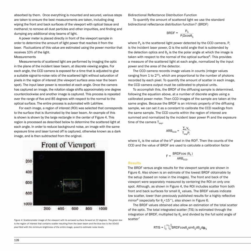
128

absorbed by them. Once everything is mounted and secured, various steps are taken to ensure the best measurements are taken, including drag wiping the front and back surfaces of the viewport with optical tissue and methanol; to remove all dust particles and other impurities, and finding and dumping any additional stray beams of light. A power meter is placed directly in front of the viewport sample in order to determine the amount of light power that reaches it from the laser. Fluctuations of this value are estimated using the power monitor that receives 10% of the light. Measurements Measurements of scattered light are performed by imaging the optic in the plane of the incident laser beam, at discrete viewing angles. For each angle, the CCD camera is exposed for a time that is adjusted to give a suitable signal-to-noise ratio of the scattered light without saturation of pixels in the region of interest (the viewport surface area near the beam spot). The input laser power is recorded at each angle. Once the camera has captured an image, the rotation stage shifts approximately one degree counterclockwise and another image is captured. This process is repeated over the range of five and 85 degrees with respect to the normal to the optical surface. The entire process is automated with LabView. For each image, a region of interest (ROI) was selected that corresponds to the surface that is illuminated by the laser beam. An example of this is shown is shown by the large rectangle in the center of Figure 4. This region is processed as described below to determine the scattered light at each angle. In order to reduce background noise, an image with the same exposure time and laser turned off is captured, otherwise known as a dark image, and is then subtracted from the original.

Figure 4: Scatterometer image of the viewport with its arrowed surface forward at 22 degrees. The green box is the region of interest that contains scatter resulting from the laser beam and the blue box is the 50x50 pixel field with the minimum brightness of the entire image, qused to estimate noise levels.

Bidirectional Reflectance Distribution Function To quantify the amount of scattered light we use the standard bidirectional reflectance distribution function7 (BRDF)

where PS is the scattered light power detected by the CCD camera, Pi is the incident laser power, Ω is the solid angle that is subtended by the detection optics and θS is the the polar angle at which the image is taken with respect to the normal of the optical surface6. This provides a measure of the scattered light at each angle, normalized by the input power and the area of the detector. The CCD camera records image values in counts (integer values ranging from 1 to 216), which are proportional to the number of photons recorded by each pixel. To quantify the amount of scatter in each image, the CCD camera output must be calibrated to physical units. To accomplish this, the BRDF of the diffusing sample is determined, following the equation above, at a number of discrete angles using a calibrated power meter. Then CCD images of the sample are taken at the same angles. Because the BRDF is an intrinsic property of the diffusing sample, we can set it as a constant to calibrate the CCD readings from the same sample. The CCD counts within the region of interest are summed and normalized by the incident laser power Pi and the exposure time of the camera Texp,

where Vk is the value of the kth pixel in the ROI6. Then the counts of the CCD and the value of BRDF are used to calculate a calibration factor

ResultsThe BRDF versus angle results for the viewport sample are shown in Figure 6. Also shown is an estimate of the lowest BRDF obtainable by the setup (based on noise in the images). The front and back of the viewport were separately measured by centering the ROI on only one spot. Although, as shown in Figure 4, the ROI includes scatter from both front and back surfaces for small θs values. The BRDF values indicate low scatter, lower than previously published results for a highly reflective mirror6 (especially for θs<15°), also shown in Figure 6. The BRDF values obtained also allow an estimation of the total scatter of the optic. The total integrated scatter (TIS) is estimated through the integration of BRDF, multiplied by θS and divided by the full solid angle of scatter7

BRDF = PS

PiΩcosθS

ARBCCD =∑kVk

TexpPi

F = BRDFcos (θS )

ARBCCD

RTIS = ∫0 ∫0 BRDFcosθSsinθSdθSd S2π 2

129

where R is the reflectivity of the optic and S is the azimuthal scattering angle. Here, independence of BRDF to the azimuthal scattering angles is assumed because the viewport is smoothly polished and therefore expected to scatter isotropically. The total integrated scatter (TIS) of the viewport for angles 5 through 85 was 0.9ppm for the front surface and 0.9ppm for the back. For comparison, the highly reflective mirror had a TIS of 3.8ppm from angles 9 to 85.

ConclusionThis Advanced LIGO viewport optic was found to have an average BRDF of less than 10−6 for 5 to 85 degrees. This is a very low level of scatter, the lowest measured at the CSUF scatter lab to date. The low scatter of this viewport should help reduce the risk of noise from stray light in Advanced LIGO.

AcknowledgementsThis work was supported by the National Science Foundation awardPHY-0970147 and the LSAMP research grant HRD-0331537.

References“Gravitational Waves: Sources, Detectors and Searches,” Keith Riles, Progress in Particle & Nuclear Physics 68 (2013) 1

J. R. Smith for the LIGO Scientific Collaboration, “The path to the enhanced and advanced LIGO gravitational-wave detectors,” Class. Quantum Grav. 26,114013 (2009).

“Hulse and Taylor win Nobel Prize for discovering binary pulsar” Bertram Schwarzschild, Physics Today; Dec93, Vol. 46 Issue 12, p17 (1993)

“Predictions for the rates of compact binary coalescences observable by ground-based gravitational-wave detectors,” J Abadie et al (the LIGO Scientific Collaboration and Virgo Collaboration) Class. Quantum Grav. 27 173001 (2010).

“Impact of Unconverted Scattered Light on Advanced Interferometric gravitational wave detectors” D Ottoway, P Fritschel, S Waldman, Optics Express 20 8329 (2012).

“Large-angle scattered light measurements for quantum-noise filter cavity design studies,” Fabian Magana-Sandoval, Rana X. Adhikari, Valera Frolov, Jan Harms, Jacqueline Lee, Shannon Sankar, Peter R. Saulson, and Joshua R. Smith, JOSA A, Vol. 29, Issue 8, pp. 1722-1727 (2012).7 J. C. Stover, Optical Scattering, 2nd edition (SPIE Optical Engineering Press, 1995).

Figure 5 Scatter data of both the front and the back of the viewport, the high reflective mirror [from 5] for comparison and the BRDF noise limit of the setup. This limit rises at 32, 33, and 59 degrees along with the BRDF from the viewport; hinting that the rise is not due to scatter, but to stray light in the lab or a defect in the set-up.

130

BIOGRAPHIES

Auriana Arabpour is a third year molecular and biotechnology major. Her research ranges from scientific interpretation of family dynamics in terms of cortisol analysis to the role of lysosomes in iron metabolism and pathway. She plans to pursue medical school after graduating Cal State Fullerton as well as continuing her research.

Jenny C. Chang will be graduating with a B.A. in Mathematics, with a concentration in Applied Mathematics, in May 2013. She is a CSUF President’s Scholar, Ronald E. McNair Scholar, Southern California Edison Scholar, and a member of the Louis Stokes Alliance for Minority Participation. She has had the pleasure of working with Dr. Sam Behseta on statistical modeling of neurons and being able to present her research at conferences. As a Supplemental Instruction Leader for the CSUF Math Department, Jenny enjoys helping students taking historically difficult math courses. She holds executive board positions for the President’s Scholars Student Association as well as the S.M.A.R.T. Girls Support Group. Upon graduation, she will be joining the Business Career Foundation Program at The Boeing Company. In the future, she hopes to return to school to obtain a Master’s in Mathematics and become a community college professor.

As a second year college student, Andres Cisneros got recruited to a marine lab. He worked with faculty mentor Danielle Zacherl. Andres studied larval settlement patterns in the Olympia oyster, Ostrea lurida. The following year Andres got accepted to The Southern California Ecosystem Program (SCERP) where as a SCERP scholar Andres is investigating the effects of a restored oyster bed on the local clam community.

AUTHORS

131

Lauren Dorough is a senior at CSUF and will graduate with a B.S. in Biological Science with a Biodiversity, Ecology, and Conservation Biology concentration in May, 2013. She is a scholar in the Southern California Ecosystems Research Program (SCERP) at CSUF and attributes much of her success to being given the opportunity to partici-pate in the program. She is passionately interested in vertebrate ecology and conservation biology and plans to pursue a professional position that will allow her to continue to study these subjects. In May of 2012, she was the recipient of the Dr. and Mrs. Donald B. Bright Environmental Scholarship. She won an Outstanding Poster Presen-tation award at the Society for the Advancement of Chicanos and Native Americans in Science (SACNAS) national conference in October, 2012 for a poster presentation of the research on bats presented here. After graduation, she plans to pursue a career as a wildlife biologist and hopes to later receive her M.S. in ecology related field.

Asha Cyrs will graduate in 2014 with a B.A. in Mathematics. Her love for numbers and puzzles have brought her to the world of geometry. Under the direction of her advisor, Dr. Suceava, she completed undergraduate research that investigated inequalities obtained from the isoperimetric inequality for planar curves. Dr. Suceava’s back-ground in geometry is what helped the research paper flourish and be successful.

Holly Eeg is a graduating Earth Science and Anthropology student and is currently researching the paleoclimate of the Mojave Desert under adviser Dr. Matthew Kirby and CSUF's Paleoclimatology and Paleotsunami Laboratory. She is an advocate for cross-discplinary research, specifically geoarchaeology, GIS applications and paleoenvironmental change. Her other research interests include human origins, archaeometry and obsidian-sourcing, some of which she has collaborated and presented posters on at various anthropology conferences during her undergraduate career. Holly is excited to continue learning about the geological sciences and looks forward to pursuing a MSc geology degree in the near future.

Rebecca Etnyre is a fourth-year undergraduate student working on her B.A. in Mathematics with a concentration in Applied Mathematics. Her love for numbers, the three-dimensional world, and teaching has inspired her to continue research and studies in Differential Geometry all while in preparation to become a high school mathematics teacher. Recently, she finds herself involved in the Fullerton Mathematical Circle, where she and a team of undergraduates prepare students in grades 2-12 for Mathematical Competitions. By looking at how students might prepare for these exams and how they choose to answer, the paper completed about the Fullerton Mathematical Circle has been featured in an Outreach Poster presentation at the 2013 Joint Mathematics Meetings in San Diego,CA.

132

Brian Giolli is a senior majoring in biochemistry at California State University, Fullerton. He is currently working with Dr. Madeline Rasche researching methanogenic pathways and plans on obtaining a master's degree. His ultimate goal, however, is to attain a professional position within the industry for the direct purpose of performing research.

Reina Galvez will graduate in 2013 with a B.A. degree in Mathematics, Probability and Statistics. Her interest in marine science and love for mathematics has led her to statistics; a field she can combine both of her passions to build a career. Working with Dr. Sam Behseta, Reina and her team have been focusing on a statistical analysis of the neuronal firings rates recorded from the primary motor cortex of a monkey’s brain. She and her team were recognized with an “Outstanding Presentation Award” for their work at the 2013 Joint Mathematical Meetings.

Brittany Grassbaugh will graduate in 2014 with a B.S. in Biochemistry and is looking forward to earning her PhD. As a student at Fullerton Community College, she was awarded a spot in the 2011 HHMI Summer Research Program at CSUF. Her experiences in Dr. Melanie Sacco’s molecular biology laboratory helped to confirm her desire to pursue a research career. She transferred to CSUF in the fall and continued her work on the tomato 14-3-3 protein throughout the school year. The next summer, she was accepted to the MIT Summer Research Program. This intensive nine-week program gave her the opportunity to work in Dr. Michael Strano’s chemical engineering laboratory. Her project involved optimizing a carbon nanotube biosensor gel that detects protein interactions. She is currently a two-year HHMI Scholar and works under her advisor, Dr. de Lijser, on the mechanistic studies of oximes in his organic chemistry laboratory.

Cody Gruebele is a senior majoring in Applied Mathematics at California State University, Fullerton. He is currently working with Dr. Angel R. Pineda on fat/water separation of magnetic resonance images (MRI) using various models and numerical techniques. His interests include model building, numerical analysis, and differential equations. His plans are to attend Cal State Fullerton's masters program in Applied Math this fall and hopes to pursue a career in industry thereafter. He would like to thank his research advisor, Dr. Angel R. Pineda, for his continued assistance and guidance throughout the project, and his girlfriend Shelby for her nonstop support.

133

Julie Hofstra is a senior who is working on her B.S. degree in Chemistry after transferring from Cerritos College as a CSU Edison Scholar. She was a recipient of the Glenn Nakaya Scholarship and the Undergraduate Award for Achievement in both Organic Chemistry and Analytical Chemistry following her first year at CSUF. She is also the treasurer of the Chemistry and Biochemistry Club and a member of the Golden Key International Honor Society and University Honors Program. She currently works in the research laboratory of Dr. Paula Hudson where she studies atmospheric photochemistry in collaboration with Dr. Peter de Lijser. Julie has presented her work at the 2012 Southern California Conference for Undergraduate Research at CSU Channel Islands as well as the 2013 Informal Symposium on Kinetics and Photochemical Processes in the Atmosphere at Caltech. She also serves as a Supplemental Instruction leader for the Department of Chemistry and Biochemistry and wants to enter a career in teaching after attending graduate school.

Natalie Hollis is a senior undergraduate B.S. geology major at CSU Fullerton. She is currently president of the Geology Club, and chair of the Natural Sciences and Mathematics Interclub Council (NSM-ICC). She has been working on her research with advisor Diane Clemens-Knott since the beginning of her 2nd year at CSUF and is looking into the age, origin, and lateral variation of detrital zircons in the Peninsular Ranges forearc basin. She has presented her research multiple times in poster sessions at professional meetings such as the American Chemical Society (ACS), American Association of Petroleum Geologists (AAPG), and the Geological Society of America (GSA) National Meeting. As a final presentation, she is looking to present her research in an oral presentation at the GSA - Cordilleran Section meeting in May 2013. She plans to graduate in May 2013, continue on in academia by attending graduate school to receive an M.S. degree, and hopes to one day receive a PhD.

Quinn Howard is currently in her third year at California State University Fullerton. She is a double major in Molecular Biology and Dance. Her current research consists of family stress management via biological markers. She plans to practice medicine after graduating.

Antouneo Kassab will graduate in 2013 with a B.A. in Mathematics, Probability and Statistics. As a Supplemental Instruction Leader in the Mathematics Department, he still finds time to participate in research under the instruction of Dr. Sam Behseta. Antouneo and his team are learning about parametric and non-parametric methods to model neuronal firing rates in the primary motor cortex of the brain. At the 2013 Joint Mathematical Meeting in San Diego, he and his team presented their work and were recognized with an "Outstanding Presentation Award". After graduation from CSU, Fullerton, he plans to continue his education by attending a graduate program and earn my M.S. degree in Statistics. Antouneo has enjoyed every math class he has taken and can’t wait to learn more.

134

(Eric Kessler) I grew up with an interest in the sciences and as my academic career has progressed I have concen-trated in biology, specifically biodiversity, ecology, and conservation. Currently I am working with faculty mentor Dr. Kristy Forsgren studying endocrine-disrupting compounds in waste-water and their impact on the reproductivephysiology and social behavior of the blackeye goby, a sequential hermaphrodite. I am also doing concentration-exposure studies on zebrafish using an insecticide and herbicide prevalent in our coastal waters that may have endocrine disrupting properties. Recently, I co-presented a poster from the SCERP summer group projectinvestigating predation risk of artificial bird nests in coastal sage scrub and associated edges near natural and suburban habitats at the 2012 SACNAS conference, in Seattle, WA.

Taylor Kennedy is a California native from Huntington Beach. His love for geology was discovered when working toward his Associate of Arts degree at Orange Coast College. Taylor is finishing his thesis and will graduate from California State University Fullerton with a Geol Sci degree this fall. Taylor also works for his teacher Professor Laton and pursues an active life performing martial arts and suffers through mudruns.

Duy Ngo is a mathematician with concentration in statistics, and graduated Fall 2012. Working as Supplemental Instructor Leader and facilitator in the Fullerton Mathematical Circle project had cultivated his interest in teaching. He was also active in doing research in Dr. Behseta’s lab and presenting his research in many conferences. His poster presentation which collaborated with other two colleagues won the Outstanding Presentation Award MAA Undergraduate Poster Session at Joint Mathematics Meetings in San Diego, California.

Aaron Ninokawa is a President’s Scholar double majoring in Biology (Marine Bio) and Chemistry (Environmental Chem) and minoring in Mathematics. At Cal State Fullerton, he currently works in Dr. Paula Hudson’s atmospheric chemistry lab studying the interactions of aerosol with water. He will be graduating in the spring of 2013.

135

Brayan Ortiz will graduate 2013 with a B.A. degree in Mathematics. He will be continuing his passion for the ap-plication of mathematics and statistics in graduate school starting fall of 2013. Under the Minority Access to Re-search Career’s (MARC) program, Dr. Mortaza Jamshidian, Professor of Mathematics and Statistics at CSUF, has been advising him throughout a statistical validation of a cognitive test. This work has been in collaboration with Dr. Ahmad Khatoonabadi, from the Tehran University of Medical Sciences. Brayan has presented this research at various conferences, but most notably won awards at the national conferences SACNAS 2012 and JMM 2013.

Lucy Odom will be graduating in Spring 2013 with a B.A. degree in Applied Mathematics. She is interested in not only the applications, but also in the theoretical aspect of Mathematics. Under the direction of Dr. Bogdan Suceava, she co-authored two papers that went into publication. The first paper was “An Elementary View on Gromov Hyperbolic Spaces,” and it will appear in the online journal Forum Geometricorum. The second paper she co-authored was “New Curvature Inequalities for Hypersurfaces in the Euclidean Ambient Space,” which will appear in the Taiwanese Journal of Mathematics. Lucy also did an undergraduate summer research program at UCLA in the summer of 2012, with a project titled “Dendritic Cell Immunotherapy for Melanoma.” Aside from research, Lucy has also been involved with the Math Club, the Fullerton Math Circle, tutoring, grading, and leading a mathematics workshop to supplement coursework in Calculus courses at CSUF Mathematics Department.

Cinthia Padilla is a McNair and LSAMP scholar that will be graduating in the Spring of 2013 with a B.S. in Physics. She first became interested in physics in high school and decided to pursue an academic career in the intriguing field. She has conducted research under the advisement of Dr. Joshua Smith for about three years and completed a project for the Laser Interferometer Gravitational Wave Observatory (LIGO) Scientific Collaboration (LSC) pertain-ing to the light scattering of an Advanced LIGO viewport. Conducting experimental research has inspired Cinthia to use her knowledge of physics to pursue a graduate degree in mechanical engineering. She has been able to present her research at several conferences that include the SACNAS national Conference, among others, and has been able to do so with the help of the Luis Stokes Alliance for Minority Participation program (LSAMP).

Emily Ramos is a Senior in the Mathematics department. Her research experience began when Dr. Gulhan Bourget took Emily under her. As a result of Dr. Bourget's mentoring, Emily has grown and gained a new respect for mathematics. During Intersession 2013, Emily traveled to Thailand with 5 fellow CSUF students to conduct research on HIV. This past year, she has been working with Dr. Bourget in comparing F statistics and Hotelling's T2 statistics with regard to Microarray Experiments. After graduating this May, Emily intends on continuing her education; the goal is obtaining a PhD in Biostatistics. Realizing that she can make a difference, even if it is a small fraction of a difference, is well worth the time and effort.

136

Nicholas is a senior at California State University Fullerton studying pure and applied mathematics. He will gradu-ate in Spring 2013 and will pursue graduate level study thereafter. Currently he is doing research with Dr. Zair Ibragimov on polynomial isometries of the p-adic integers and properties of polynomials in finite fields. When he finishes a PhD program Nicholas wants to teach at the university level and continue to do research in pure and possibly applied mathematics.

Amissi Sadiki is hoping to graduate in fall 2013 with a B.S in Biochemistry. What interested him the most about his research topic was its vast real-life applications. Renewable sources of energy is a hot topic in this generation, not only for environmental reasons, but also for reducing our nation’s dependence on non-renewable energy such as fuel. Under the supervision of Dr. Haan, Amissi was able to investigate the use of electrochemistry to enhance fuel cell technology, which is a renewable source of energy. In addition, this is his first publication in addressing this issue, and he hopes to further investigate and work with fuel cells in the remainder of the year.

Dylan Tennant is a Southern California Ecosystems Research Program (SCERP) Scholar completing her undergrad-uate independent research project under advisor Dr. Paul Stapp. She will graduate in May 2013 with a B.S. in Bio-logical Sciences with a concentration in Biodiversity, Ecology, and Conservation. Dylan’s research interests focus on the ecology of mammals and after graduation plans to begin a career as a wildlife biologist. She has presented this research at the Southern California Academy of Science (SCAS) 2012 Annual Meeting in Los Angeles, CA, and she received a travel scholarship to present at the Society for the Advancement of Chicanos and Native Americans in Science (SACNAS) 2012 National Conference in Seattle, WA.

Cole Wheadon will be graduating in Spring 2013 with a B.S. degree in Biochemistry. He has been working under the guidance of Dr. Linder for the last year and a half focusing on the intestinal uptake of copper and iron. After graduating from CSUF, Cole plans to attend and complete pharmacy school, a goal that he has been aiming towards since high school.

137

EDITORS

Neha Ansari is a second-year undergraduate student at Cal State Fullerton pursuing a Bachelor of Science in bio-chemistry and a minor in print journalism. Neha recently began working in Dr. Peter de Lijser’s organic chemistry lab where she studies the reactive intermediates of oxime radicals. Aside from participating in research, Neha also is a member of the University Honors Program and is one of Cal State Fullerton’s President’s Scholars. Upon graduation, she intends to pursue a PhD in chemistry and enter a career in the industry or become a professor and conduct her own research at a university. Neha enjoys serving as the Chemistry and Biochemistry Section Edi-tor for Dimensions because it combines her two passions of science and journalism and looks forward to continu-ing to work for Dimensions during her remaining time at CSUF.

Chris Baker (Editor-in-Chief) is an undergraduate student attending CSUF, with plans to attain a B.S. in geological sciences. Currently, he is working with Dr. Phil Armstrong on determining the exhumation rates of the southern Alaskan mountain ranges, through the use of fission track dating. After attaining a B.S. he plans to continue to graduate school to attain his M.S. and Ph.D. He transferred to CSUF in the fall of 2011 from Cypress and Fullerton Community Colleges, and currently is an officer in the South Coast Geological Society.

Erik Cadaret is a fifth year undergraduate student soon to graduate this spring with a Bachelor of Science degree in Geology. He has spent the past several years doing research in the Mojave Desert that relates to groundwater resources for the Mojave Water Agency (MWA). Erik has done geologic research in Thailand through the Environ-mental Science Research in Thailand (ESRT) program here at CSUF, attended several weeks of Western Michigan University Hydrogeology Field Camp, helped rebuild houses in St. Bernard Parish, New Orleans with AmeriCorps, worked with inner city youth in New York City, and regularly attends professional meetings and conferences. As of late, he will be continuing his studies in geology and will be attending graduate school to obtain a Master of Sci-ence degree in Hydrogeology at University of Nevada, Reno – Desert Research Institute this fall.

138

Tiffany Le is an award winning graphic designer gradutating Spring 2013 with a B.F.A. in Graphic Design. She specializes in editorial design, advertising, packaging, and branding and hopes to pursue a career in editorial design.

Kelly Hartmann is graduating Spring 2013 with a B.A. in Mathematics, Teaching. With the help of Dr. CadwalladerOlsker she was able to research student development of proof schemes. Working with Dr. Suceava, as part of Fullerton Math Circle she was able to develop a passion for teaching gifted students. She is currently pursuing research in teaching linear relationships with Dr. Kimani. Kelly has also been involved in S.M.A.R.T. Girls Support Group, Math Club, Supplemental Instruction, tutoring, and grading. In the fall Kelly plans to start the credential program at CSUF.

Nick Tran is a Biology major with a concentration in Cellular and Developmental Biology. He has a double minor in Mathematics and Chemistry. As a SCERP Scholar (an NSF-funded program; Southern California Ecosystems Research Project), he does paid research relating to sexual behavior of invertebrates. His main research focus has to do with the effects of senescence and size on sperm quality. He has presented research on the plant diversity of the Chaparral microhabitat of Southern California and hope to publish his findings on sexual behavior later this year. After CSUF, he hopes to gain admission into an MD-PhD program where he can begin his work on aging and regeneration.

Robert Wright is a CSUF physics senior with ambitions of pursuing a career in the aerospace industry. In his time at CSUF he has been honored with receiving the Robert W. Kedzie, and Physics Department Outstanding Achievement awards. He is an active member of the Natural Sciences and Mathematics Inter Club Council and is deeply involved with experimental optics research under the advisement of Dr. Joshua Smith.




DIM

ENSIO

NS


the journal of undergraduate research in natural sciences

Documents