The Kids Are OK: Divorce and Children’s Behavior Problems

JUI-CHUNG ALLEN LI

WR-489

May 2007

This paper made possible by the NIA funded RAND Center for the Study of Aging (P30AG012815) and the NICHD funded RAND Population Research Center (R24HD050906).

WORK ING P A P E R

This product is part of the RAND Labor and Population working paper series. RAND working papers are intended to share researchers’ latest findings and to solicit informal peer review. They have been approved for circulation by RAND Labor and Population but have not been formally edited or peer reviewed. Unless otherwise indicated, working papers can be quoted and cited without permission of the author, provided the source is clearly referred to as a working paper. RAND’s publications do not necessarily reflect the opinions of its research clients and sponsors.

is a registered trademark.

The Kids Are OK: Divorce and Children’sBehavior Problems1

Jui-Chung Allen LiRAND Corporation

May 4, 2007

1Support for this research was provided by the National Institute of ChildHealth and Human Development (HD 29550) and by a Dean’s Dissertation Fel-lowship from the Graduate School of Arts and Science at New York University, andis gratefully acknowledged. I also appreciate comments and suggestions from LarryWu, Tom DiPrete, Willie Jasso, Dalton Conley, Kathleen Gerson, Larry Busch,Tom Dietz, Christine George, Min-Hsiung Huang, Su-Jen Huang, Arie Kapteyn,Jacob Klerman, Tony Tam, and Chris Winship.

Abstract

Although social scientists and commentators agree that parents should be

responsible for their children’s well-being and keep their children’s interest in

mind when they consider the possibility of ending a marriage, they disagree

on how much the association between parental divorce and child well-being

is causal. This paper reexamines the causal claim that parental divorce is

detrimental to children’s emotional well-being, measured in terms of behavior

problems. I analyze panel data from the 1986-2002 waves of Children of the

National Longitudinal Survey of Youth 1979. As in previous research, I find

that parental divorce is associated with a higher level of behavior problems

in children in the ordinary least squares regressions that adjust for observed

factors. However, once I control for selection on unobserved factors that

are either constant over time or change at a constant rate over time by

using generalizations of the child fixed-effects model, the effect of divorce

substantially declines and is no longer statistically significant. I conclude

that children of divorce would have fared equally well/poor in terms of their

emotional well-being if their parents had remained married.

For most people, the really pressing question they are likely to

wrestle with at some point in their lives is . . . “Should I stay mar-

ried, maybe even for the sake of the kids?” This heartfelt debate

is central to the future of marriage as a permanent commitment.

And it is a debate that is taking place, not only among people

but within people.—Waite and Gallagher (2000)

To speak of fostering an emotional democracy does not mean be-

ing weak about family duties, or about public policy towards the

family. Democracy means the acceptance of obligations, as well as

rights sanctioned in law. The protection of children has to be the

primary feature of legislation and public policy. Parents should

be legally obliged to provide for their children until adulthood, no

matter what living arrangement they enter into.—Giddens (2003)

Divorce and child well-being is a highly contentious social science question

that interests the general public and policymakers alike. Commentators

across the ideological and political spectrums have all agreed that parents

should be responsible for their child’s well-being. Hence, they should take

into account their child’s well-being when contemplating a family decision,

among which divorce is perhaps the most serious (Giddens 2003; Waite and

Gallagher 2000). Yet these views implicitly suppose that (changes in) family

structure is a cause of the differentials in child well-being; however, if there

were in fact no causal link between divorce and child well-being, there would

be no scientific basis for public policy concern or social intervention.

Indeed, this belief that family structure plays a causal role in determin-

ing child well-being has been well articulated in the sociological literature, as

1

demonstrated in the three recent presidential addresses delivered by sociolo-

gists to the Population Association of America. Waite (1995) argued that, on

the average, marriage provides numerous benefits for both adults and chil-

dren that alternative family arrangements do not. Her argument has been

taken as providing a scientific foundation for supporters of policies intended

to promote marriage. Cherlin (1999) reviewed similar issues with a narrower

focus on children and concluded that, while the observed correlations cannot

be the entire story, family structure matters for child well-being. McLanahan

(2004) detailed how family changes that impact different social strata differ-

ently might be responsible for the diverging trend in social inequality for

children from different backgrounds. Perhaps, not surprisingly, the position

of these eminent scholars represents where the current empirical literature

stands. Although many social scientists suspect that selection plays a role in

the correlation between family structure and child well-being, few studies to

date have convincingly challenged the belief in the causal claim that children

would fare better if their parents stay/become married. Indeed, some even

argue that social scientists will forever debate about the causation between

family structure and child well-being until a randomized experiment can be

conducted (McLanahan and Sandefur 1994:11); however, ethical concerns

will never allow such an experiment to happen.

Although causation is best established using randomized experiments, I

argue that the evidence in this paper seriously questions the consensus that

divorce and child well-being are causally linked by explicitly and rigorously

modeling unobserved factors that may differentially select families into di-

vorce. I reexamine the causal claim that divorce is detrimental to children’s

2

emotional well-being (measured in terms of overall behavior problem), using

multiwave panel data to eliminate selection biases from unobserved confound-

ing factors, an issue that is not adequately addressed in prior research. I dis-

cuss two distinct sets of theoretical mechanisms through which the selection

may operate and adjust for selection in two ways, by using the fixed-effects

models and by using generalizations of such fixed-effects models that incorpo-

rate individual-specific linear trends. I also use longitudinal data that yields

larger sample sizes than are found in most research to date; thus, the analysis

in this paper will have reasonable statistical power to detect effects of divorce

even under a fixed-effects or individual-specific linear trend specification.

Once selection on unobservables is controlled, I find no effect of divorce

on children’s behavior problems. This null finding suggests that divorce it-

self is not the culprit for the lower emotional well-being children of divorce

experience. Indeed, these findings suggest that to help children of divorce,

social scientists and policymakers should seek to understand the process both

before and after marriages come apart (Furstenberg and Cherlin 1991) and

target interventions on proximate determinants of socioemotional develop-

ment, rather than attempt to prevent divorce itself.

PRIOR RESEARCH

Social scientists have consistently found that children of divorce have, on av-

erage, lower well-being than children in two-parent families, after adjusting

for socioeconomic background and other demographic factors (Amato 2000;

McLanahan and Sandefur 1994; Seltzer 1994). These findings, however, are

taken by many social scientists and commentators (especially those trying

3

to translate these findings for non-scholarly audiences) (Popenoe 1996; Mar-

quardt 2005) as evidence that divorce causes reductions in children’s well-

being, despite repeated warnings about the difference between association

and causation. Thus, public controversies about divorce and child well-being

typically reflect a disagreement (often implicit) over whether divorce causes

observed differences in well-being between children of divorce and children

in families with two biological parents.

Early research on the effect of divorce on children has largely been based

on clinical samples, and sometimes such research has even lacked a control

group. The findings from such research lack external validity and are, thus,

difficult to generalize. Nonetheless, two early longitudinal studies based on

unrepresentative samples offered important insights on potential selection

issues by finding that many children of divorce had already been having

various emotional disturbances, adjustment problems, and substance abuse

problems prior to the disruption of their parents’ marriages (Block et al.

1986; Doherty and Needle 1991).

In a seminal paper, Cherlin and colleagues (1991) highlighted the impor-

tance of a prospective design. They noted two potential sources of selection

that had been overlooked in previous empirical work: marital conflicts and

family dysfunction. Their findings yielded smaller effects of parental divorce

after controlling for pre-disruption family conditions and a pre-disruption

measure of child well-being, suggesting that previous estimates of the effects

of divorce were upwardly biased by not adequately addressing these selection

issues. Their study, thus, suggests that despite the robust and relatively

strong association between divorce and child well-being documented in vari-

4

ous cross-sectional studies, there is far less empirical evidence in support of

a causal role of divorce, given the relative lack of studies using longitudinal

data and methods that would allow researchers to address these selection

issues (Ni Bhrolchain 2001).

The findings by Cherlin et al. (1991) have led many social scientists to

conclude that parental divorce is causally linked to reductions in children’s

emotional well-being, but that the degree of harm is less than that indicated

in the associations found in cross-sectional studies. Nonetheless, a detailed

examination of the literature since Cherlin et al. (1991) suggests that this

conclusion is more inconclusive than is sometimes acknowledged. Cherlin

et al. (1991) followed an entire cohort of British 7-year-olds until they were

11 in the National Child Development Study, controlling for social class, race,

scores of the same outcome measured at age 7, a health visitor’s report of fam-

ily problems and difficulties, and a physician’s report of physical handicap,

mental retardation, or emotional maladjustment measured at age 7. They

also presented results from a parallel analysis examining only children’s be-

havior problems using data from the U.S. National Survey of Children (NSC);

the respondents were slightly older than the British children (age 7-11 at base

survey) interviewed in 1976 and followed up in 1981. The effect of parental

divorce for boys dropped by about a half and was no longer statistically sig-

nificant from the model controlling for social class, race, whether the mother

was employed outside the home, to a model adding child’s behavior problem

in 1976 and parental marital conflicts. However, they noticed an unusual

pattern for girls, with girls of divorced parents showing somewhat fewer be-

havior problems than girls of continuously married parents, and they were

5

cautious about this unusual finding. In contrast, Baydar (1988), also ana-

lyzing the same NSC data but using an advanced dynamic statistical model

described in Tuma and Hannan (1984), found that entering a stepfamily after

divorce, but not parental divorce itself, reduces certain aspects of children’s

emotional well-being in a five-year window between 1976 and 1981.

Morrison and Cherlin (1995) focused on a two-year window between 1986

and 1988 in Children of the National Longitudinal Survey of Youth 1979

(NLSY79). They found that controlling for pre-disruption child outcomes

drove down the coefficient of marital disruption to zero for girls (although

the initial level of difference was not statistically significant), but that it did

not change the coefficient for boys. The effect of parental divorce on boys’

behavior problems was partly explained by the decline in economic resources.

Morrison and Coiro (1999) examined how much the effect of divorce interacts

with parents’ marital conflicts, using child and parent data from the 1988-

1994 waves of NLSY79. They found that, holding constant pre-disruption

level of behavior problems, marital conflict and marital disruption both in-

creased children’s behavior problems. Moreover, their results suggested that

children with high-conflict parents who remained married to each other had

the highest level of behavior problems. Jekielek (1998), using the 1988-1992

wave of the same data as Morrison and Coiro (1999), found that children

in high-conflict families have a lower level of anxiety and depression if their

parents divorced, which is inconsistent with the findings reported in Morrison

and Coiro (1999).

Sun (2001) analyzed data from the 1990-1992 waves of National Educa-

tion Longitudinal Study (NELS) and found a small, but statistically signif-

6

icant, effect of divorce on adolescents’ self-reported behavior problems after

controlling for pre-disruption behavior problems. In addition, he found no

association between divorce and teacher-reported behavior problems or ado-

lescent substance use after controlling for pre-disruption measures of family

relations and parental characteristics.

Painter and Levine (2000) examined the effect of parental divorce during

a child’s high-school years on a white, non-Hispanic subsample in the 1988

NELS, which followed a sample of 8th graders through 1994. They found

that, at the base 1988 survey, children whose parents were to divorce in the

next few years exhibited higher levels of emotional and behavior problems

than had children whose parents were continuously married during subse-

quent waves. However, they did not find significant differences in family

economic conditions, parents’ education, and parenting behaviors between

the two groups of children prior to divorce. Controlling for the above pre-

disruption characteristics slightly reduces the association between parental

divorce and high-school dropout and substantially reduces the association

between parental divorce and out-of-wedlock childbearing.

Furstenberg and Teitler (1994) found that children of divorce had lower

education, economic well-being, and psychological well-being and that con-

trolling for pre-disruption factors—including child characteristics, family back-

ground, quality of parents’ marital relations, and parent-child relations—

substantially reduces the association between divorce and subsequent child

well-being.

Although longitudinal data allow researchers to control for pre-disruption

child outcomes, many studies using longitudinal data have not exploited this

7

opportunity (e.g., Allison and Furstenberg 1989; Carlson and Corcoran 2001;

Peris and Emery 2004). Although these studies provide useful descriptions

that help unravel the complex family transitions (Carlson and Corcoran 2001)

and the process of divorce (Lansford et al. 2006; Strohschein 2005; Sun and

Li 2002; VanderValk et al. 2005; Wu et al. 2006), their findings provide no

rigorous evidence for any causal link between divorce and child well-being.

In sum, several prior longitudinal studies have relied on non-representative,

clinical samples ; as a result, their results may not generalize. Among studies

using data collected from a probability sample, many have not controlled for

pre-disruption child outcomes and, thus, have not exploited the advantage

of panel data in making causal inference . Even studies using longitudinal

data have used multiwave panel data for descriptive purposes, providing lit-

tle direct statistical control of selection biases; or have only analyzed two

waves of data in their panel design. Several studies examining marital con-

flict often obtained different findings, despite using the same data source .

Finally, the handful of studies that might be thought to provide evidence for

a “causal” effect of parental divorce have sometimes yielded conflicting find-

ings and have analyzed narrow age ranges for children, short periods during

which divorce can occur, or an over-representation of young children born to

young parents from disadvantaged socioeconomic circumstances .

THEORY

Causal Mechanisms of Parental Divorce

A variety of theoretical mechanisms exist by which marital disruption might

lower children’s well-being. One such mechanism focuses on parental re-

8

sources, with divorced parents being less able, on average, to provide suffi-

cient resources to fulfill children’s social, economic, and emotional needs than

families with two biological parents (Seltzer 1994). Divorce often entails mov-

ing to a different location, transferring to a new school, and adopting to an

unfamiliar life routine, all of which may diminish the well-being of children

following divorce (McLanahan and Sandefur 1994). Children’s adjustment

can also be affected by stressful events as the custodial parent copes with

being single, resumes dating, moves in with a new partner, and remarries

(often to another person with children). Family change and instability may

be another source of stress, which may, in turn, be causally linked to prob-

lem behaviors for children of divorce (Fomby and Cherlin 2007; Hao and Xie

2002; Wu and Martinson 1993; Wu and Thomson 2001).

Divorced families often experience a substantial and sudden decline in

economic circumstances (Peterson 1996; Weitzman 1985), which McLana-

han and Sandefur (1994) have argued is responsible for about half the dis-

advantage for children of divorce. The difficulty of making ends meet, com-

pounded by frustrations with delayed or missing child support payments,

imposes additional burden on divorced mothers. In addition, mothers’ emo-

tional reactions toward economic difficulties may be transmitted to children

passively through parent-child interactions and actively through the child’s

social learning.

Psychologically, the sudden departure of a parent may affect a child’s

sense of security and a child’s sense of being able to control his/her envi-

ronment. The behavioral manifestation of psychological harm may be seen

in a child’s distress, anxiety, social withdrawal, irritability, and frustration

9

(Wallerstein and Blakeslee 2003). The divorced parents’ inability to fulfill

their children’s emotional needs may be exacerbated by the stress associated

with protracted inter-parental conflicts (Cherlin et al. 1991). Separated par-

ents may continue to fight over the division of property, child custody, and

various other matters, not only during separation but sometimes long after

a divorce is finalized (Furstenberg and Cherlin 1991). Parents in conflict

also can serve as negative role models from which children learn to express

their emotions in an inappropriate way, which, in turn, exacerbate behavior

problems in children of divorce (Grych and Fincham 1990).

Selection Mechanisms

It is worth noting that the resources that parents are able and willing to

provide for their children may vary dramatically across marriages and across

divorces. There are “good” parents and “bad” parents, just like there are

“good” spouses and “bad” spouses. It is plausible that a “bad” spouse or par-

ent may well have been a “bad” spouse or parent prior to marital disruption

(and may, thus, have been a factor in causing the disruption); the alternative

hypothesis—that a spouse or parent turned “bad” after the disruption—is

perhaps less plausible. If so, this is one mechanism by which presumed “con-

sequence” of marital disruption may potentially be a precursor to it (Cherlin

et al. 1991). Although divorced families, on average, are disadvantaged on

various social and emotional measures relative to intact families, many of

these disadvantages might well have been present had the parents remained

married. If these disadvantages (e.g., parental conflict, family dysfunction,

disengaged parenting) had been present irrespective of the parent’s legal sta-

10

tus or the presence or absence of a parent, child well-being may not have

differed if the parents had remained married or if they had divorced.1 In

other words, to make a causal claim about the effect of parental divorce

implies that we must address, theoretically, what would have happened to

the causal mechanisms of the family if the parents—who were divorced—had

remained married. For divorce to have a causal effect on child well-being,

some causal factor that accompanies divorce must change before and after

divorce and the change must take place in a way that causes child well-being

to deviate from its pre-divorce trajectory. Conversely, if there is no change in

a causal factor affecting child well-being, observed differences in well-being

for children of divorce will reflect the selection of families of divorce on these

factors, which I will refer to as “static selection on time-invariant factors.”

Furthermore, a potential causal factor can change pre- and post-divorce but

not alter the child’s pre-disruption trajectory of well-being; the change in this

causal factor will represent what I will refer to as “dynamic selection.” I give

several examples below to illustrate these two possible selection mechanisms.

Static Selection on Time-Invariant Factors

“Static selection” will occur if an unobserved factor exists that remains un-

changed before and after divorce but is associated with a higher risk of di-

vorce. One possible static selection mechanism is through the social inheri-

tance or genetic transmission of personality traits (Freese et al. 2003). For

example, certain aspects of child temperament are relatively stable across de-

1Note that economic resources typically do decline following a divorce; hence, child well-being would decline after divorce if the effect of declining economic resources on children’sbehavior problems outweighed the effects of socioemotional factors.

11

velopmental stages and associated with parental personality traits possibly

through heredity (van den Oord and Rowe 1997). If a child with a difficult

temperament is also likely to have parents with divorce-prone personality

traits (Jockin et al. 1996), the child will both be exposed to a higher risk of

parental divorce and behavior problems. If so, a naive estimate of the effect

of divorce that ignores this type of selection will be upwardly biased.

While a decline in income is often a consequence of divorce (Peterson

1996; Weitzman 1985), persistent poverty is likely to increase the risk of

marital disruption. Similar stress mechanisms that operate in low-income di-

vorced families may operate in low-income married families and cause higher

levels of children’s problem behaviors through long-term elevated levels of

inter-parental conflicts. Low-income families also tend to live in poor neigh-

borhoods with relatively low-quality schools. Poor neighborhood conditions

or poor school quality may cause the children to develop higher levels of be-

havior problems (Harding 2003). If low income, high divorce rates, and high

levels of children’s behavior problems were to covary in these ways, a naive

estimate of the effect of divorce that ignores selection on economic conditions

prior to divorce is likely to be biased upwards.

The intensity and frequency of inter-parental conflict has been repeatedly

cited as a key risk factor that may impair the socioemotional development

of children (see, e.g., the review of studies by Grych and Fincham 1990). If

high-conflict marriages have a higher propensity to divorce and high levels

of marital conflict cause children to develop behavior problems, then these

factors will also be sources of selection bias.

Because the majority of divorces stem from low-conflict marriages (Booth

12

and Amato 2001), one might question the importance of selection on mari-

tal conflict. However, divorce-prone, low-conflict marriages may be harmful

for children’s emotional well-being if parents in such marriages are disen-

gaged. Loveless and/or disengaged parents, even in a materially affluent and

low-conflict household, may still cause problems in children’s socioemotional

development. Suggestive evidence along these lines can be traced to the fa-

mous Harlow experiments of nearly a half century ago (Harlow 1958; 1959),

in which infant monkeys deprived of parental warmth had severe develop-

mental deficits, even though they were adequately fed. These results and a

subsequent body of research have led developmental psychologists to believe

that adequate socialization requires engaged parenting. Nevertheless, there

is substantial variation empirically in father’s time and activities with his

children both among intact families (Harris et al. 1998; Yeung et al. 2001)

and after marital disruption (King 1994; King et al. 2004). This suggests

that marital disruption is not the mechanism that may diminish the degree

of a father’s care and attention to his children. If loveless and disengaged par-

enting reflects the loss of interest of a parent in the marriage, failing to take

into account the selection on parental involvement will again upwardly bias

naive estimates of the effect of divorce on children’s emotional well-being.

Dynamic Selection

As noted above, I refer to “dynamic selection” when a potential causal fac-

tor changes over time but remains on its previous trajectory (i.e., with a

constant slope). Dynamic selection may occur either through the contempo-

raneous effect of a time-varying factor or through the cumulative effect of a

13

time-invariant factor. Consider a first scenario in which the level of marital

conflict is associated with the likelihood of divorce and in which we observe

marital conflict increases as the marriage condition worsens. Increasing level

of inter-parental conflict may have a contemporaneous effect, increasing lev-

els of problem behaviors (e.g., aggression or depression) of children through

mechanisms of observational learning (Bandura 1977) or lack of parental dis-

cipline. This scenario, although similar to the static selection on conflict,

will lead to a trending, rather than time-constant, effect of selection. Simply

holding constant a fixed level (or the intercept) will not properly eliminate

the biases from the dynamic selection.

Consider a second scenario in which marital conflict remains at a constant

level but in which the influence of marital conflict on children’s problem

behaviors is cumulative over time, which again will yield a trending effect of

selection. Children may also develop behavior problems gradually because

of the loveless parent-child relationship and they lack an appropriate parent

role model, with behavior problems diverging over time for children in high-

conflict, loveless families and for children in low-conflict, loving families if

the effect of marital conflict is cumulative. This scenario will also lead to

a dynamic selection effect, which implies a model controlling only for static

selection mechanisms will be misspecified, with the standard fixed-effects

yielding an upwardly biased estimate for the effect of divorce.

Virtually all previous studies have assumed that the selection mecha-

nisms have a static, time-invariant effect on children’s emotional well-being;

under such an assumption, when the pre-disruption child outcome is sampled

is irrelevant. However, if dynamic selection is present, controlling only for

14

static selection will yield biased and inconsistent estimates; hence, it will be

necessary to specify a model that accommodates dynamic selection.

STATISTICAL MODELS AND HYPOTHE-

SES

Standard Regression Adjustment

I begin the analysis of this paper using standard ordinary least-squares (OLS)

regression estimates to replicate results reported in prior research, in which

researchers have found that divorce is strongly associated with children’s

behavior problems. The variables in this replication include nearly all the

variables that have been used in the previous research.

Following the cross-sectional designs of much previous work, I do not

exploit any longitudinal features of the panel design in this first replication

attempt. Hence, this replication takes the form of pooled cross-sectional

data with “standard regression adjustment”—or the “analysis of covariance”

(Winship and Morgan 1999)—estimated by OLS techniques. Formally, the

model can be written as follows:

yit = β · xit + θi · Dit + εit (1)

where yit is the measure of children’s emotional well-being (specifically, be-

havior problem index, in this case), Dit is a time-varying dummy indicator

for parental separation/divorce (whichever comes first), and xit is the vector

of socioeconomic and demographic control variables. This analysis addresses,

as did those analyses reported in previous studies, the question of whether

children of divorce fare emotionally worse than children whose parents are

15

continuously married—coming from similar socioeconomic and demographic

characteristics. If the sample characteristics and the distributions of the in-

dependent variables, dependent variable, and control variables in this replica-

tion are similar to those previous studies on divorce and children’s behavior

problems, I should find coefficients of comparable magnitudes.

Fixed-Effects Model

In Model 1 above, the coefficient for parental divorce E(θi) can be interpreted

causally only if the underlying assumptions hold. However, if static selection

on time-invariant unobservables (e.g., child temperament, persistent poverty)

is present, then Model 1 will be subject to omitted variable bias and will yield

an inconsistent estimate of the effect of divorce.

To formalize the argument, consider the specification of a fixed-effects

model that incorporates a child-specific, time-invariant unobserved compo-

nent, ci:

yit = β · xit + θi · Dit + ci + υit (2)

Comparing Models 1 and 2 shows that εit = ci + υit. Thus, if ci and Dit are

correlated, the naive OLS regression adjustment estimator for Model 1 will

yield an inconsistent estimate for E(θi), the effect of divorce. In other words,

if children of divorce are subject to the static selection, then the coefficient

of E(θi) under the fixed-effects model in Model 2 should be smaller than that

under the standard regression adjustment in Model 1.

The fixed effects, ci, is identified when there are repeated measures of yit.

To estimate (2), I apply a time-demeaned transformation, yielding

(yit − yi) = β · (xit − xi) + θ · (Dit − Di) + (υit − υi), (3)

16

which can then be estimated by OLS (Wooldridge 2002).

Random Trends Model, I

As noted above, we often may suspect that both dynamic and static selection

mechanisms are present. If so, then the estimator for the coefficient E(θi) in

(2) will overstate the effect of divorce in the presence of dynamic selection.

To deal with this possibility, I further relax the assumption on the error term

υit in (2) by including a unique slope, gi, for each individual child:

yit = β · xit + θi · Dit + ci + gi · t + ωit. (4)

This model is called the “random trends model” (Wooldridge 2002). The

model in (4) generalizes (2) by letting υit = gi · t + ωit. Hence, if gi is

correlated with parental divorce Dit, then the estimate of E(θi) in Model 2

will be inconsistent. In the presence of dynamic selection, the true effect of

parental divorce may be even smaller than those estimated in the first two

analyses.

One can estimate the random trends model by taking two transformations

followed by OLS estimation. A first step is to take first differences between

adjacent observations:

Δyit = β · Δxit + θ · ΔDit + gi + Δωit. (5)

A second step is to apply the time-demeaned transformation to obtain the

fixed-effects estimator, which eliminates gi:

(Δyit − Δyi) = β · (Δxit − Δxi) + θ · (ΔDit − ΔDi) + (Δωit − Δωi). (6)

One then applies OLS to the expression in (6).

17

Random Trends Model, II

A potentially undesirable feature of the random trends model is that the

time-path of behavior problems for each child is assumed to follow one and

only one child-specific slope. Hence, the model assumes that, for children

of divorce, the slope before parental marital disruption is the same as the

slope after disruption. This specification, in effect, borrows strength from

both the pre- and post-disruption data to estimate a single slope for each

child—yielding a potentially biased estimate of the slope and, thus, the other

coefficients. To investigate this possibility, I estimate a second random trends

model:

yit = β · xit + θi · Dit + γi · (Dit · Uit) + ci + gi · t + ωit (7)

where Uit is the duration since divorce. Adding the interaction between

divorce and duration since divorce allows children of divorce to have a post-

disruption slope that differs from the pre-disruption slope by the magnitude

of γi.

Typically, I will not have enough data to estimate two different slopes

for an individual child. Instead, I estimate an average post-disruption slope,

E(γi), for all children. This post-disruption coefficient, and how other co-

efficients are affected by including this coefficient, will provide a sensitivity

check for the equal-slope assumption in the first random trends model in (4).

DATA

In studying the effects of parental divorce on child well-being, I exploit a

unique design of the National Longitudinal Survey of Youth 1979 (NLSY79)—

18

the availability of a wealth of longitudinal data on all children born to women

in the original NLSY79 sample that can be linked to equally rich data for

their biological coresident mothers in the original NLSY79. Children living in

the same households as the NLSY79 women were surveyed every other year

since 1986. Although the child sample cannot be regarded as a probability

sample of any cross-section of the U.S. population, it is representative of bio-

logical children born to women living in the United States in 1979 who were

born between 1957 and 1964. The longitudinal and intergenerational design

of the NLSY79 mother-child sample is especially suitable for examining the

effects of parental divorce on children. However, a limitation of these data

is that findings can be only generalized to children living with their mother

after a marital disruption and not to children in other living arrangements

after parental divorce. The analysis includes all waves of data up to 2002.

Behavior Problem Index

The outcome variable is the behavior problem index (BPI)—a commonly

used indicator for children’s socioemotional development in both scholarly

work and clinical applications. Behavior problems are also an established

predictor of educational attainment and socioeconomic status (McLeod and

Kaiser 2004; Miech et al. 1999). Understanding the relationship between

parental divorce and children’s behavior problems may help explain the rela-

tionship between family structure and social inequality (Biblarz and Raftery

1999). The behavior problem index has been documented to exhibit substan-

tial continuity across the life course (Knoester 2003; Loeber 1982; Sampson

and Laub 1992). Children of divorce consistently score higher on the BPI

19

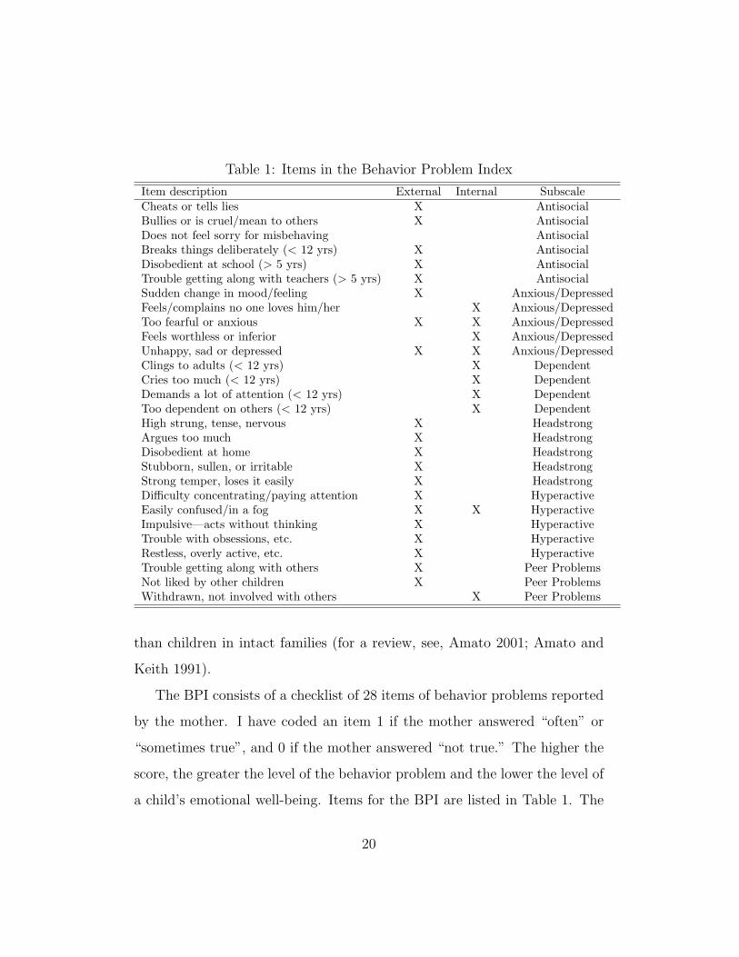
Table 1: Items in the Behavior Problem Index

Item description External Internal SubscaleCheats or tells lies X AntisocialBullies or is cruel/mean to others X AntisocialDoes not feel sorry for misbehaving AntisocialBreaks things deliberately (< 12 yrs) X AntisocialDisobedient at school (> 5 yrs) X AntisocialTrouble getting along with teachers (> 5 yrs) X AntisocialSudden change in mood/feeling X Anxious/DepressedFeels/complains no one loves him/her X Anxious/DepressedToo fearful or anxious X X Anxious/DepressedFeels worthless or inferior X Anxious/DepressedUnhappy, sad or depressed X X Anxious/DepressedClings to adults (< 12 yrs) X DependentCries too much (< 12 yrs) X DependentDemands a lot of attention (< 12 yrs) X DependentToo dependent on others (< 12 yrs) X DependentHigh strung, tense, nervous X HeadstrongArgues too much X HeadstrongDisobedient at home X HeadstrongStubborn, sullen, or irritable X HeadstrongStrong temper, loses it easily X HeadstrongDifficulty concentrating/paying attention X HyperactiveEasily confused/in a fog X X HyperactiveImpulsive—acts without thinking X HyperactiveTrouble with obsessions, etc. X HyperactiveRestless, overly active, etc. X HyperactiveTrouble getting along with others X Peer ProblemsNot liked by other children X Peer ProblemsWithdrawn, not involved with others X Peer Problems

than children in intact families (for a review, see, Amato 2001; Amato and

Keith 1991).

The BPI consists of a checklist of 28 items of behavior problems reported

by the mother. I have coded an item 1 if the mother answered “often” or

“sometimes true”, and 0 if the mother answered “not true.” The higher the

score, the greater the level of the behavior problem and the lower the level of

a child’s emotional well-being. Items for the BPI are listed in Table 1. The

20

BPI scores are collected biennially for children ages 4 and over until 1992.

From 1994 onward, they are collected for children between 4 and 15 years

of age. I restrict my analysis to only measurements taken for children under

age 15 at the time of the interview. Because of this age constraint, there are

up to 6 repeated BPI measures with intervals of roughly 2 years apart for

each child. I use the summated raw score of BPI (hence, the range of the

scale is 28) and control for the age pattern using sex-specific linear splines

with a node at 9.5 years of age.2

Figure 1 presents the density histograms (with normal curves imposed)

of the BPI scores. On average, boys have almost 1 more behavior problem

than girls (with respective means of 8.7 and 7.9). The distributions of scores

are slightly skewed, but log-transformations do not make the distributions

look “more normal.”

Control Variables

I include controls for the child’s demographic characteristics. The child’s

sex is coded 1 for boys and 0 for girls. The child’s race and ethnicity are

measured by two mutually exclusive dummy variables, coded 1 for black and

for Hispanic, with non-black-non-Hispanic being the reference category. The

birth order and the mother’s age at the child’s birth are included as contin-

2Although prior research typically used an age-standardized BPI score for the depen-dent variable, Cronbach (1990) has shown that this common practice will lead to biasedestimate of the effect of divorce if parental divorce is correlated with child’s age (p. 242).Because a fundamental demographic insight on exposure and probability suggests thatmore and more children will experience a parental divorce as they age, parental divorcewill be correlated with child’s age, suggesting that an age-standardized score is inappro-priate. Instead, I control for the age- and sex- specific pattern of change in BPI usingcovariates on the right-hand side of the equation, rather than using standardization on theleft-hand side of the equation.

21

Figure 1: Distributions of Behavior Problem Index Score0

.02

.04

.06

.08

Den

sity

mean−1 s.d. +1 s.d. +2 s.d.Behavior Problem Index

Boys (Mean=8.69, S.D.=5.98)

0.0

2.0

4.0

6.0

8.1

Den

sity

mean−1 s.d. +1 s.d. +2 s.d.Behavior Problem Index

Girls (Mean=7.87, S.D.=5.65)

Distributions of BPI by Child’s Gender

uous variables. I also include of the mother socioeconomic and demographic

characteristics, including mother’s nativity, education, total family income

at her first marriage, mother’s age at first marriage, age at first birth, mother

was raised as a Catholic, mother’s religiosity in 1979, mother had her first sex

before age 20, mother’s family structure at age 14, any regular reading ma-

terials in mother’s household when she was at age 14, mother’s self-esteem

measured in 1980 and AFQT percentile score, and dummy indicators for

missing data on self-esteem and AFQT. These variables are invariant over

time.

I also include several time-varying control variables. Child’s age (in

22

months) is measured at the time of each assessment of the behavior prob-

lem.3 Number of siblings changes value at each wave of child assessment

in the same way as I measure the age of child. I also constrain the value

for number of siblings to stop accumulating after a parental separation (or

divorce if there is no reported separation before a divorce).

Sample Restrictions

I restrict the NLSY79 mother sample to ever married women as of the 2002

interview, deleting all men and never married women.4 Among ever married

women, I delete those who are childless as of 2002 or with missing data on

age at first birth (N = 739). I also delete those women with missing data on

family structure at age 14 (N = 8), reading materials at age 14 (N = 39),

Catholic religion (N = 13), religiosity (N = 4), age at sex (N = 72)5,

education at marriage (N = 10), total net family income at the formation

of first marriage (N = 13), family income at the formation of first marriage

(N = 13), and the reason first marriage was dissolved (N = 46).6

The full child sample is matched to the mother sample, as restricted by

the above criteria, with the exception of 404 children who were born outside

3Because there are two modes of data collection of the child assessment data, i.e., amother supplement and a child supplement, the age of child in each survey year has twoversions corresponding, respectively, to the supplements. For behavior problems, age ofchild corresponds to the child’s age when the “mother supplement” was administered.

4The status of never married, like other time-varying statuses (such as childlessness)is partly affected by sample attrition. If a respondent was no longer interviewed after acertain survey year and was never married as of the last survey interview, she would beconsidered “never married” and hence deleted from the current analysis even if she mighthave gotten married between the last time we interviewed her and the 2002 survey.

5This is primarily because of a noninterview in all three consecutive surveys between1983 and 1985 in which the question was fielded.

6Most of them are those whose first marriages dissolved before the 1979 survey, inwhich only information on reasons the most recent marriage ended was recorded.

23

the mother’s first marriage (i.e., either before her first marriage formation or

after her first marriage dissolved) and who were excluded from the analysis.

I further deleted observations taken when the child was more than 15 years

of age at the time of survey interview because only pre-1994 surveys have

BPI measures for children age 15 and over, who tend to be born to relatively

young mothers. Finally, listwise deletion of missing data on the dependent

variable of BPI drops 802 observations. This gives a sample of 6,332 children

born to 3,124 mothers.

Strengths and Weaknesses of Data

A common criticism about the Children of NLSY79 data has been the way

the sample is generated. These children enter the sample through birth to

the original NLSY79 mother sample and do not represent any cross-section

of children in the U.S. population. In particular, the early waves of the

child sample tended to over-represent children born to younger mothers with

disproportionately low socioeconomic background. However, as the sample

of mothers and children has “aged”, the child sample has grown increas-

ingly more representative with respect to age structure and socioeconomic

background. Table 2 illustrates this point by displaying the patterns of ob-

servations across survey waves. In 1986, all mothers in the analytic sample

were under age 24 when they gave birth to the child. By the 2002 wave, the

oldest mothers were 40 years of age, which is about the range we typically

see in the population. As a result, using the 1986-2002 waves of the child

data in this paper improves on analyses of the same data in prior studies

both because of larger sample sizes and because of representativeness.

24

Table 2: Design Features of Children of the NLSY79

Mom’s child’s Age of Child at Survey Yearage at birth birth cohort ’86 ’88 ’90 ’92 ’94 ’96 ’98 ’00 ’02

8–15 1973 13 15 . . . . . . .9–16 1974 12 14 . . . . . . .10–17 1975 11 13 15 . . . . . .11–18 1976 10 12 14 . . . . . .12–19 1977 9 11 13 15 . . . . .13–20 1978 8 10 12 14 . . . . .14–21 1979 7 9 11 13 15 . . . .15–22 1980 6 8 10 12 14 . . . .16–23 1981 5 7 9 11 13 15 . . .17–24 1982 4 6 8 10 12 14 . . .18–25 1983 . 5 7 9 11 13 15 . .19–26 1984 . 4 6 8 10 12 14 . .20–27 1985 . . 5 7 9 11 13 15 .21–28 1986 . . 4 6 8 10 12 14 .22–29 1987 . . . 5 7 9 11 13 1523–30 1988 . . . 4 6 8 10 12 1424–31 1989 . . . . 5 7 9 11 1325–32 1990 . . . . 4 6 8 10 1226–33 1991 . . . . . 5 7 9 1127–34 1992 . . . . . 4 6 8 1028–35 1993 . . . . . . 5 7 929–36 1994 . . . . . . 4 6 830–37 1995 . . . . . . . 5 731–38 1996 . . . . . . . 4 632–39 1997 . . . . . . . . 533–40 1998 . . . . . . . . 4

25

Table 3: Number of Observations per Child

Obs. / child Number of children Percent Cumul. Percentage1 807 12.7 12.72 967 15.3 28.03 1,005 15.9 43.94 1,386 21.9 65.85 1,803 28.5 94.36 364 5.7 100.0

Total 6,332 100.0

Also, note that because the BPI is measured between age 4 and 15 and

because the survey takes place only every two years, there are at most six

observations for any child. Thus, children born to the oldest and youngest

mothers will have fewer than six observations because of the design of the

original survey. Survey nonresponse also yields an unbalanced panel for some

children despite extremely low sample attrition in the mother-child data.

Table 3 gives the distribution of the number of observations per child. Close

to 90 percent of the children have two or more observations, which is required

for estimating the child fixed-effects models. Over 70 percent of the children

have three or more observations, which is required for estimating the two

random-trends models.

The unbalanced panel data might create a methodological problem if

sample attrition and survey nonresponse are correlated with parental divorce.

Table 4 provides a closer look at the patterns of these panel data for children

of divorce and children in intact families. In any wave (from 1986-2002,

thus, a maximum of 9 observations per child), the symbol “x” represents

26

observations with valid data of the dependent variable of BPI, and the symbol

“.” represents either no data (structurally) or missing data (nonresponse).

The top 20 frequent patterns for each group, which capture about three

quarters of the respondents for each group, do not appear to be any different.

RESULTS

I conduct parallel analyses on the full analytic sample, on the sample of

children with at least two observations, and on the sample of children with

at least three consecutive observations. Although the OLS regressions can

be estimated on all these subsamples, the random-trends models can only be

estimated on the subsample of children with at least three observations. Sim-

ilarly, the child fixed-effects models can only be estimated on the subsample

of children with at least two observations. To facilitate comparisons across

models, I only present results based on at least three consecutive observa-

tions. I obtain similar results regardless of the sample restrictions imposed

(see Appendix).

Descriptive statistics

Table 5 presents descriptive statistics for children’s characteristics by the

child’s sex and whether the mother was divorced. Children of divorce belong

disproportionately to younger mothers and to racial and ethnic minorities.

Table 6 presents descriptive statistics for the mothers of the children by their

status of divorce as of the 2002 survey. Divorced women are more likely

to be black and Hispanic, to have grown up in a broken family, to be from

27

Table 4: Patterns of Panel Data by Parental Separation/Divorce

Intact Family Divorced FamilyFrequency Percent Pattern Frequency Percent Pattern

249 6.6 . . . . . . . . x 263 10.2 xx . . . . . . .231 6.2 . . . . . . xxx 223 8.7 xxxxx . . . .224 6.0 . . . . xxxxx 215 8.4 xxxx . . . . .219 5.8 . . xxxxx . . 192 7.5 . xxxxx . . .212 5.6 . . . . . xxxx 142 5.5 . . xxxxx . .204 5.4 . . . . . . . xx 128 5.0 xxx . . . . . .189 5.0 . xxxxx . . . 101 3.9 . x . . . . . . .181 4.8 xxxxx . . . . 81 3.1 . . . xxxxx .160 4.3 . . . xxxxx . 76 3.0 . . . . xxxxx157 4.2 xxxx . . . . . 65 2.5 x . . . . . . . .153 4.1 xx . . . . . . . 62 2.4 . . . . . xxxx137 3.7 . x . . . . . . . 59 2.3 . xxxxxx . .69 1.8 xxx . . . . . . 49 1.9 . . . . . . xxx68 1.8 . . xxxxxx . 45 1.8 . . xxxxxx .67 1.8 . . . . . . x . x 40 1.6 . . . xxxx . .67 1.8 . xxxxxx . . 39 1.5 . xxx . . . . .64 1.7 . . . . xxx . x 39 1.5 . xxxx . . . .63 1.7 . . . xxxx . . 37 1.4 x . xx . . . . .60 1.6 . . . xxxxxx 33 1.3 . . xxxx . . .54 1.4 . . . . . xx . x 31 1.2 xx . x . . . . .928 24.7 (other patterns) 656 25.5 (other patterns)3756 100.0 2576 100.0

28

Table 5: Descriptive Statistics for Children of the NLSY79

Variable Girls BoysIntact family Divorced family Intact family Divorced family

Black .13 .23 .14 .22Hispanic .19 .23 .18 .26Birth order 1.79 1.80 1.79 1.79

(.90) (.92) (.86) (.90)Mom’s age at 25.78 23.43 25.65 23.48child’s birth (4.05) (4.13) (3.98) (4.02)

N 941 738 1,021 742

lower socioeconomic backgrounds, to have scored lower on the AFQT test

on cognitive ability, to have lower levels of education completed, and to have

married and have had a first child at a slightly younger age.

Age Patterns of Behavior Problem Index

Because BPI varies substantially with age, I use two methods to explore

and control for this relationship. A first exploratory method uses a variable

span “super smoother” developed by Friedman (1984). It is a nonparametric

method that helps identify the age pattern of BPI with minimal assumptions

about the bivariate relationship between age and BPI. The second method

models the multivariate relationship between age and BPI by using a linear

spline for age with a knot at 9.5 years of age, where the placement of the

knot is guided by the nonparametric analyses. The use of a spline speci-

fication is a flexible parametric method and will be used as the basis for

subsequent analysis. The results from the two methods are roughly similar,

suggesting that a spline specification provides a reasonable approximation

to the underlying age patterns (as shown in the nonparametric smoother) in

29

Table 6: Descriptive Statistics for NLSY79 Mothers

Variable Continuously Married Separated/DivorcedHispanic .18 .24Black .14 .24Foreign Born .08 .07Intact family at age 14 .78 .66Mother only at age 14 .11 .16Stepmother-father at age 14 .02 .02Stepfather-mother at age 14 .05 .09mag, papers, lib card in HH at age 14 .49 .39Raised as Roman Catholic .43 .37Frequency of religious activity in 1979 3.58 3.38

(1.66) (1.71)AFQT percentile score 48.17 35.17

(27.20) (24.17)Age at 1st sex< 20 .02 .03< 12 years of schooling at Mar1 .11 .2112 years of schooling at Mar1 .36 .3913-15 years of schooling at Mar1 .26 .28> =16 year of schooling at Mar1 .27 .12age at 1st marriage as of 2002 21.89 20.15

(3.44) (3.07)age at 1st birth as of 2002 23.88 21.21

(4.34) (3.99)Self esteem, 1980 32.59 31.86

(3.91) (3.81)N 1,037 911

30

the regression analysis.

For boys, BPI first increases and then decreases with age, with a peak

around 9.5 years of age (Figure 2). The BPI for girls follows a similar, but

much less curvilinear, pattern (Figure 3). Boys tend to have more behavior

problems than girls at all ages, which confirms the descriptive statistics on

mean levels. Children of divorce consistently have higher levels of behavior

problems. The differences are roughly the same across all ages and are more

than 1.5 points for boys and more than 1 point for girls on the BPI scale.7

Results from Regressions Adjusting Observables

I begin by estimating the naive OLS model ignoring any possible selection

on unobservables, which I refer to henceforth as results obtained from OLS

regression adjustment. The resulting pooled cross-sectional estimates in the

first and third columns of Table 7 show that parental divorce is associated

with a 1.63-point increase in boys’ behavior problems (t = 6.04, p < .0001)

and a 1.39-point increase in girls’ behavior problems (t = 5.79, p < .0001).

As expected, both associations are highly significant, indicating children of

divorce, on the average, have worse emotional well-being than their counter-

parts of the same age, sex, and race/ethnicity in intact families.

Controlling for socioeconomic and demographic factors that may con-

found the relationship between divorce and children’s behavior problems re-

duces the coefficient to 1.16 for boys (t = 4.30, p < .0001) and to 0.98 for

girls (t = 4.08, p < .0001; both with the same magnitude of standard errors).

7To gauge the sensitivity of these results to the observation plan, I replicated the sameanalysis on samples with at least one observation per child, two observations per child,and three observations per child. The results are indistinguishable from each other.

31

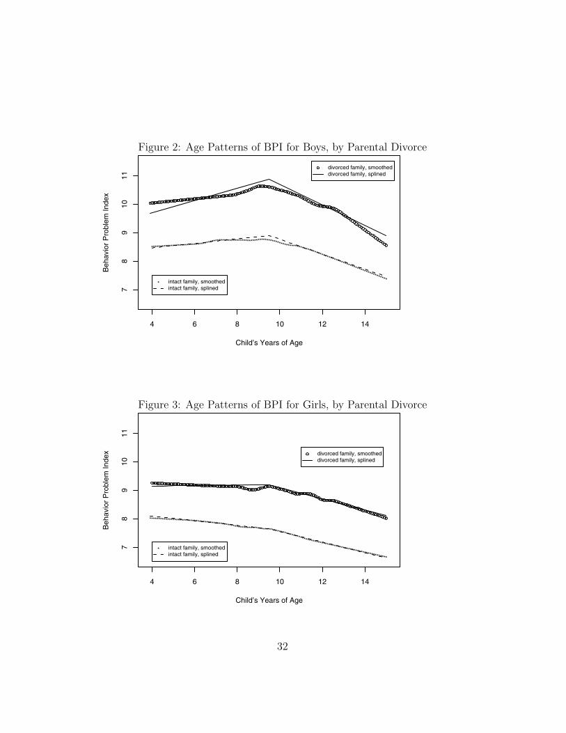
Figure 2: Age Patterns of BPI for Boys, by Parental Divorce

4 6 8 10 12 14

78

910

11

Child’s Years of Age

Beh

avio

r P

robl

em In

dex

***************************************

*********************************************************************************************** intact family, smoothed

intact family, splined

divorced family, smootheddivorced family, splined

Figure 3: Age Patterns of BPI for Girls, by Parental Divorce

4 6 8 10 12 14

78

910

11

Child’s Years of Age

Beh

avio

r P

robl

em In

dex

**************************************************************************************************************************************

* intact family, smoothedintact family, splined

divorced family, smootheddivorced family, splined

32

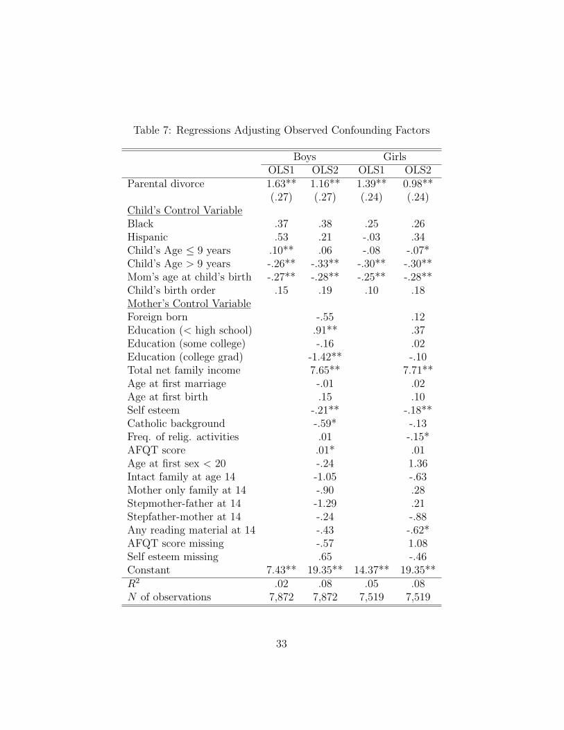
Table 7: Regressions Adjusting Observed Confounding Factors

Boys GirlsOLS1 OLS2 OLS1 OLS2

Parental divorce 1.63** 1.16** 1.39** 0.98**(.27) (.27) (.24) (.24)

Child’s Control VariableBlack .37 .38 .25 .26Hispanic .53 .21 -.03 .34Child’s Age ≤ 9 years .10** .06 -.08 -.07*Child’s Age > 9 years -.26** -.33** -.30** -.30**Mom’s age at child’s birth -.27** -.28** -.25** -.28**Child’s birth order .15 .19 .10 .18Mother’s Control VariableForeign born -.55 .12Education (< high school) .91** .37Education (some college) -.16 .02Education (college grad) -1.42** -.10Total net family income 7.65** 7.71**Age at first marriage -.01 .02Age at first birth .15 .10Self esteem -.21** -.18**Catholic background -.59* -.13Freq. of relig. activities .01 -.15*AFQT score .01* .01Age at first sex < 20 -.24 1.36Intact family at age 14 -1.05 -.63Mother only family at 14 -.90 .28Stepmother-father at 14 -1.29 .21Stepfather-mother at 14 -.24 -.88Any reading material at 14 -.43 -.62*AFQT score missing -.57 1.08Self esteem missing .65 -.46Constant 7.43** 19.35** 14.37** 19.35**R2 .02 .08 .05 .08N of observations 7,872 7,872 7,519 7,519

33

Consistent with prior findings, these coefficients in the regression adjustment

are of substantially smaller magnitudes (with a reduction of approximately

one-third) than the simple correlations reported earlier, but the coefficients

remain highly significant.8 These estimates, thus, are similar to those in

previous studies, such as the findings reported by McLanahan and Sandefur

(1994), who concluded that children of divorce are worse off compared with

children in two-parent families of similar socioeconomic and demographic

backgrounds.

The magnitudes of the effects suggest that an “average” divorced mother

will notice one more behavior problem in their child than their married coun-

terpart with similar socioeconomic backgrounds, on a scale of mean of about

8 items on a checklist of 28 items. The effect size (0.19 standard deviations

for boys, and 0.17 standard deviations for girls) is similar in magnitude to

that reported in the meta-analysis by Amato and Keith (1991).

Results from Regressions Adjusting Unobservables

Columns 1 and 4 of Table 8 give estimates from the fixed-effects model spec-

ified in (2). These results show that the coefficient for parental divorce drops

to .45 for boys (t = 1.25, n.s.) and .48 for girls (t = 1.23, n.s.). Both are less

than half the magnitude of the naive estimator in columns 2 and 4 of Ta-

ble 7). Neither fixed-effects coefficient is statistically significant. Note that

the statistical insignificance in these results stems from the smaller fixed-

effects coefficients and not from the larger standard errors. Substituting the

8The standard errors are smaller in the present analysis than they were in most previousresearch and, thus, the p values for significance level are smaller because these data havethe largest number of observations and divorce and, therefore, greater statistical power.

34

Table 8: Regressions Adjusting Selections on Unobservables

Boys GirlsFE RT1 RT2 FE RT1 RT2

Parental divorce .45 -.41 -.42 .48 .44 .46(.36) (.60) (.60) (.39) (.65) (.66)

Time since divorce -.04 .09(.30) (.32)

Control VariableChild’s age ≤ 9.5 years .06 -.02 -.01 -.09* .19 .17

(.04) (.52) (.52) (.04) (.47) (.48)Child’s age > 9.5 years -.35** -.44 -.43 -.30** -.04 -.06

(.04) (.53) (.54) (.04) (.48) (.50)Constant 8.45** .22 .23 8.75** -.53 -.55

(.27) (1.05) (.95) (.27) (.95) (.95)R2 .72 .14 .14 .68 .14 .14Number of Observations 7,872 5,902 5,902 7,519 5,649 5,649

Note: All models control for a linear spline of child’s age with a node at 9.5 years.

OLS standard errors for the fixed-effects standard errors, for example, does

not yield statistical significance for boys and very marginal statistical signif-

icance for girls, showing that the lack of statistical significance is not to the

result of the loss of statistical power in the fixed-effects model.

Including the random trends yields somewhat different results for boys

but not for girls (see the RT1 models in Table 8). For boys, the coefficient

flips sign and declines further in magnitude, implying that a parental divorce

is associated with nearly half a point reduction in boys’ BPI. Although not

statistically significant, the point estimate nevertheless suggests, contrary

to most previous research, that parental divorce may improve boys’ emo-

tional well-being after controlling for dynamic selection. For girls, estimated

35

coefficients are similar in the fixed-effects and random-trends models. Over-

all, both the fixed-effects and random-trends coefficients tell a similar story:

Parental divorce has no statistically significant effect on children’s behavior

problems, with the estimated effect small enough in magnitude that fewer

than half of the divorced mothers would observe a one-item increase on the

BPI in their child.

Table 8 also shows little evidence for the possibility that the child-specific

random slope might vary before and after marital disruption. The random-

trends models with an interaction between parental divorce and the time since

marital disruption (the RT2 models in Table 8) yield nearly identical results

as the random-trends models with a single random slope. The estimates of

the interaction effect are close to zero (-.04/year for boys and .09/year for

girls, with standard errors of .30 and .32), suggesting that the slopes before

and after marital disruption, on average, are not much different.

DISCUSSION

This paper asks a straightforward question: Is the association between parental

divorce and children’s emotional well-being documented in numerous prior

studies causal? The results presented in this paper show no evidence that

parental divorce causes any increase in children’s behavior problems. While

I successfully replicate the “robust” finding about the association when con-

trolling for a wide range of the child’s and mother’s socioeconomic and family

background factors, the association disappears when I exploit the longitudi-

nal research design to eliminate selection biases on unobserved factors. De-

spite the strong belief among social scientists and the general public alike,

36

the answer to this specific causal question on divorce and children’s behavior

problems, based on the analyses in this paper, is no.

It is certainly important to clarify the qualifications for this negative

answer, since this answer challenges a vast literature on parental divorce

and children’s emotional well-being. The null finding presented is specific

to one outcome—the Behavior Problem Index—for children between ages 4

and 15, who were born within the mother’s first marriage and who resided

with the mother after divorce. It is, thus, inappropriate to extrapolate these

results beyond this age range to other outcome measures, to children living

with divorced fathers, and to children born out of wedlock or in stepfam-

ilies. For example, these results do not overturn the finding that children

in divorced families suffer from a nontrivial financial loss (Peterson 1996;

Weitzman 1985). Nor do the results provide much insight in explaining the

long-term intergenerational transmission of family behaviors (McLanahan

and Bumpass 1988). It is also important to note that the estimate is what

the methodologists call the “the average treatment effect on the treated”

(Winship and Morgan 1999).9 That is, the fixed-effects estimates in this pa-

per are intended to answer the counterfactual question of what would have

happened to children’s emotional well-being if those parents who divorced

had instead remained married. As such, these estimates say nothing about

the well-being of children born to parents who are happily married and have

rarely, if ever, pondered the possibility of a marital disruption. In fact, the

empirical analysis not only acknowledges but emphasizes the fact that chil-

9The identification of the effects relies only on data from those children whose parentsseparated or divorced in the observation period (between 1986 and 2002), not on datafrom those children whose parents were continuously married.

37

dren of divorce may differ from children in two-parent families for a variety

of reasons that might be related to their socioemotional development, the

family environment in which they grow up, and the dynamics and frailty of

their parents’ marriage. If these differences exist, the estimate for the effect

of divorce on children of divorce will not be the same as that of the effect of

divorce for an “average” child in the population.

Moving Out with a Divorce Decree

Setting aside these empirical caveats for the moment, how might we ex-

plain the findings of this paper—that parental divorce has no effect on chil-

dren’s behavioral problems—given the vast body of prior research that has

found that divorce is detrimental to children’s emotional well-being? I believe

that the consensus among researchers is correct in supposing that parental

resources are crucial in facilitating children’s socioemotional development

(Hetherington and Kelly 2002; McLanahan and Sandefur 1994; Seltzer 1994;

Waite and Gallagher 2000). They are also correct in asserting that divorced

parents have fewer social, economic, and emotional resources for their chil-

dren than parents in intact families, at least partly because of structural

barriers—e.g., separated residences and weakened parent-child ties.

Where I disagree, however, is that the divorced parents would be able to

provide equivalent parental resources as their intact-family counterparts for

the children if we were to implement a policy that, for example, prohibits mar-

ital disruption. Despite various structural barriers, not all divorced parents

are doomed to failure in their attempts to provide sufficient parental resources

needed for the healthy socioemotional development of their children—some

38

will, and others will not. By the same token, some married parents will be

able to provide sufficient parental resources needed for the healthy socioe-

motional development of their children, while others will not. Those who

will not be able to provide sufficient resources for their children tend to be

those who are more likely to divorce. Hence, attributing these differences

in parental resources to divorce requires rigorously addressing the issue of

whether these differences are indeed a consequence of divorce and, thus, an

unavoidable byproduct of marital disruption.

As I have argued in the theory section, if the behaviors that prior research

has argued are the causal factors linking parental divorce to children’s behav-

ior problems do not in fact change before and after divorce, those behaviors

in fact reflect selection, rather than causes of behavioral factors. Because

my empirical design explicitly models the influences of changes in both ob-

served and unobserved factors that may vary before and after a parental

separation, I interpret the null findings in this paper as providing solid ev-

idence for the theoretical role of selection laid out earlier. If so, then from

a policy perspective, if these selection mechanisms can be dissociated from

marital disruption, one may be able to devise policies that mitigate the con-

sequences of these selection factors without requiring that a couple remain

married. Indeed, because what marital disruption necessarily involves is a

spouse “moving out with a divorce decree.”10, reduced contact through sepa-

rate residence and a change in legal status are virtually the only things that

inevitably accompany divorce. All other things—e.g., care and money the

10In fact, even moving out is not always necessarily implied, because co-residence is nolonger taken for granted for many modern (especially professional) “married couples livingapart.”

39

non-custodial parent contributed to the child—can, in principle, be dissoci-

ated from the event of a divorce and manipulated (or remedied) following a

divorce. Thus, it is perhaps less surprising that the findings of this paper

suggest that these behaviors and child outcomes are very diverse (and, thus,

potentially malleable) for divorced parents and their children.

In summary, the findings of this paper are consistent with the selection ar-

guments contained in the speculations of Cherlin et al. (1991): The dysfunc-

tional family dynamics (possibly involving high conflicts or disengagement of

the parents) for children of divorce—the potential real cause of lower emo-

tional well-being—are likely to be present before and after marital disruption

and are unlikely to emerge only after separation. A marital separation moves

a parent out of the household and divorce brings a change in legal status,

formalizing much of what has already happened (e.g., whom the child is to

live with) and other parental obligations (e.g., visitation schedules and the

amount of child support). Neither non-coresidence nor a change in legal sta-

tus is likely to substantially change the emotional environment in which the

sensitive youthful mind is nurtured.

Although the analysis seems like attacking a straw man because no one

argues that the effect of divorce is the result of the legal paper and of the

fact that one parent no longer comes home to eat and sleep, this is nev-

ertheless what is logically implied if one holds that lower child well-being

is a causal consequence of divorce without establishing the—both necessary

and causal—link between divorce and the intervening behavior mechanisms.

Hence, that divorce might have no causal effect on children’s well-being is

not inconsistent with a view that marriages confer benefits for children’s

40

well-being, as argued by the advocates for marriage (Popenoe 1996; Waite

and Gallagher 2000) if one also acknowledges that the marriages that confer

benefits are also likely to be those that are successful and enduring.

All married couples have their ups and downs, and not every marriage

will last “’til death do us part.” It goes without saying that divorce has

existed in all the societies for all of recorded human history (Goode 1993),

which reflects the diversity of family life. If what marital disruption actu-

ally does is to selectively end those dysfunctional families—those parents

who have failed to live up to their marriage vows and play their parental

roles—while maintaining successful marriages, one might expect that child

outcomes might very well be worse for bad marriages and parents and better

for good marriages and parents, regardless of legal marital status and living

arrangements. Among severely troubled families, it may even be the case

that the “true” effect of divorce for those children whose parents ended a

“bad” marriage will be improvements in their well-being.

Speculation on Gender Differences

Although findings in this chapter point to gender differences, these findings

are difficult to interpret because the gender interactions are not statistically

significant. Nevertheless, I believe that it is perhaps worthwhile to specu-

late on these gender differences in light of the dynamic selection arguments

and empirical results from the random trends models. As shown in Table 8,

parental divorce is estimated to yield an increase of about .45 behavior prob-

lems for both boys and girls, controlling only for selection on time-invariant

effects of the unobservables. Once we control for the time-varying effects of

41

the unobservables, divorce still yields an increase of .45 behavior problems

for girls, but yields a decrease of .41 behavior problems for boys. At the risk

of overinterpreting this result, it is possible that what might lie behind this

finding11 is that the father’s absence in a dysfunctional or conflictual family

removes the negative “role model” for boys in a way that is different from the

way it affects girls, a speculation consistent with a recent study that finds

the effect of a father’s absence depends on the anti-social personality trait of

the father (Jaffee et al. 2003). If so, it may be that continuing coresidence

with mother does not change the gender-specific dynamics for girls. I leave

the test of how valid this explanation is for future research.

Policy Implications

This paper finds no evidence for an effect of parental divorce on children’s

behavioral problems, thus implying that divorce is neither harmful nor helpful

for this measure of children’s well-being. If so, a potential implication is

that public policy should be neutral with respect to marriage versus divorce.

This prescription is indeed contradictory to not only what the advocates for

marriage have argued but also to much of what is taken for granted in this

country. For policy to remain neutral with respect to parent’s legal marital

status will imply, for example, removing all the tax incentives (and penalties)

based on marital status. In other words, the standard deduction for a married

couple should simply be twice the amount for a single person. Of course, the

tax laws are just one example of potentially influenced public policies. Other

areas may include parental leave policies, welfare benefits, and so forth.

11Note that these data contain only children living with divorced mothers, and no otherliving arrangements.

42

As for the debate taking place within people, the results reported in this

paper suggest that the decision to end a marriage or stay together for the sake

of the kids would neither hurt nor help their children’s emotional well-being.

Hence, parents in an unhappy marriage should perhaps not focus on the

decision of divorce itself if they want to protect their children’s emotional

well-being. Rather, they should focus on how they can maintain, if not

improve, the level of socioemotional involvement with their children and the

level of financial contribution they make to the household in which their

children will grow up, and on how they can restrict the conflicts and their

personal sufferings away from their children. This implication indeed echoes

the observation made by psychologists about why counseling has often failed

to save a marriage (Hetherington 2002). A family is unlikely to function

well if there are “contextual factors”, such as financial difficulties, causing

strains on family members (Karney and Bradbury 2005). The detriments to

the well-being of family members caused by these other factors cannot be

improved by the status of the marriage or by the counseling sessions. To

conclude, I believe that the results of this paper and the findings of these

other researchers suggest that the direction for future research should be in

identifying what these specific proximate (or contextual) factors are and how

they work to affect the well-being of family members, rather than identifying

the effect of changes in marital status.

43

APPENDIX: SUPPLEMENTARY ANALYSIS

To make sure that decision to exclude all children with fewer than three con-

secutive observations does not change the substantive finding in Table 8, I

repeated the same analysis reported in the main text on the less-restrictive

sample with only two or more observations per child (the minimal require-

ment of child fixed-effects model). Because non-response or sample attrition

is not random, it is possible that those children who have better well-being

are more likely to remain in the sample and be interviewed multiple times in

a row. Hence, the concern is that the null finding on the effect of parental

divorce reported in Table 8 may be an artifact because the analytic sample

of at least three consecutive observations consists of those children of divorce

who are emotionally better off than those children of divorce with fewer ob-

servations. If the concern is warranted, a less restricted analytic sample will

give a larger estimate of the effect of parental divorce. Table 9 compares

the OLS and fixed-effects results based on only two or more observations

per child (top panel), the minimal data required to estimate a fixed-effects

model, with the results on at least three consecutive observations per child

(bottom panel) reported in the main text. The estimates are very similar.

Hence, the null finding appears not to be the result of restrictions on the

sample.

44

Table 9: Comparison of Two Analytic Samples

Boys GirlsOLS1 OLS2 FE OLS1 OLS2 FE

parental divorce 1.76** 1.20** 0.50 1.51** 1.00** 0.46(2+ obs./child) (0.23) (0.24) (0.33) (0.21) (0.22) (0.37)parental divorce 1.63** 1.16** 0.45 1.39** 0.98** 0.48(3+ obs./child) (0.27) (0.27) (0.36) (0.24) (0.24) (0.39)

References

Allison, Paul R. and Frank F. Furstenberg, Jr. 1989. “How Marital Disso-

lution Affects Children:Variations by Age and Sex.” Developmental Psy-

chology 25:540–49.

Amato, Paul R. 2000. “The Consequences of Divorce for Adults and Chil-

dren.” Journal of Marriage and the Family 62:1269–87.

Amato, Paul R. 2001. “Children of Divorce in the 1990s: An Update of the

Amato and Keith (1991) Meta-Analysis.” Journal of Family Psychology

15:355–70.

Amato, Paul R. and Bruce Keith. 1991. “Parental Divorce and the Well-

Being of Children: A Meta-Analysis.” Psychological Bulletin 110:26–46.

Bandura, Albert. 1977. Social Learning Theory . New York: General Learning

Press.

Baydar, Nazli. 1988. “Effects of Parental Separation and Reentry into Union

on the Emotional Well-Being of Children.” Journal of Marriage and the

Family 50:967–81.

45

Biblarz, Timothy J. and Adrian E. Raftery. 1999. “Family Strucuture, Educa-

tional Attainment, and Socioeconomic Success: Rethinking the “Pathology

of Matriarchy”.” American Journal of Sociology 105:321–65.

Block, Jeanne H., Jack Block, and Per F. Gjerde. 1986. “The Personality

of Children Prior to Divorce: A Prospective Study.” Child Development

57:827–40.

Booth, Alan and Paul R. Amato. 2001. “Parental Predivorce Relations and

Offspring Postdivorce Well-Being.” Journal of Marriage and the Family

63:197–212.

Carlson, Marcia J. and Mary E. Corcoran. 2001. “Family Structure and

Children’s Behavioral and Cognitive Outcomes.” Journal of Marriage and

the Family 63:779–92.

Cherlin, Andrew J. 1999. “Going to Extremes: Family Structure, Children’s

Well-Being, and Social Science (PAA Presidential Address).” Demography

36:421–28.

Cherlin, Andrew J., Frank F. Furstenberg, Jr., P. Lindsay Chase-Linsdale,

Kathleen E. Kiernan, Philip K. Robins, Donna Ruane Morrison, and

Julien O. Teitler. 1991. “Longitudinal Studies of Effects of Divorce on

Children in Great Britain and the United States.” Science 252:1386–89.

Cronbach, Lee J. 1990. Essentials of Psychological Testing . New York:

HarperCollins, 5th edition.

46

Doherty, William J. and Richard H. Needle. 1991. “Psychological Adjust-

ment and Substance Use among Adolescents Before and After a Parental

Divorce.” Child Development 62:328–37.

Fomby, Paula and Andrew J. Cherlin. 2007. “Family Instability and Child

Well-Being.” American Sociological Review 72:181–204.

Forehand, Rex, Lisa Armistead, and Corinne David. 1997. “Is Adolescent

Adjustment Following Parental Divorce a Function of Predivorce Adjust-

ment?” Journal of Abnormal Child Psychology 25:157–64.

Freese, Jeremy, Jui-Chung Allen Li, and Lisa D. Wade. 2003. “The Poten-

tial Relevances of Biology to Social Inquiry.” Annual Review of Sociology

29:233–56.

Friedman, Jerome H. 1984. “A Variable Span Scatterplot Smoother.” Labo-

ratory for Computational Statistics 5, Stanford University, Stanford, CA.

Furstenberg, Frank F., Jr. and Andrew J. Cherlin. 1991. Divided Families:

What Happens to Children When Parents Part . Cambridge, MA: Harvard

University Press.

Furstenberg, Frank F., Jr. and Julien O. Teitler. 1994. “Reconsidering the

Effects of Marital Disruption: What Happens to Children of Divorce in

Early ADulthood.” Journal of Family Issues 15:173–90.

Giddens, Anthony. 2003. Runaway World: How Globalization is Reshaping

Our Lives . New York: Routledge, 2nd edition.

47

Goode, William J. 1993. World Changes in Divorce Patterns . New Haven,

CT: Yale University Press.

Grych, John H. and Frank D. Fincham. 1990. “Marital Conflict and Chil-

dren’s Adjustment: A Cognitive-Contextual Framework.” Psychological

Bulletin 108:267–90.

Hao, Lingxin and Guihua Xie. 2002. “The Complexity and Endogeneity of

Family Structure in Explaining Children’s Misbehavior.” Social Science

Research 31:1–28.

Harding, David J. 2003. “Counterfactual Models of Neighborhood Effects:

The Effect of Neighborhood Poverty on High School Dropout and Teenage

Pregnancy.” American Journal of Sociology 109:676–719.

Harlow, Harry F. 1958. “The Nature of Love (Presidential Address to the

American Psychological Association).” American Psychologist 13:573–85.

Harlow, Harry F. 1959. “Love in Infant Monkeys.” Scientific American

200:68–74.

Harris, Kathleen Mullan, Frank F. Furstenberg, Jr., and Jeremy K. Marmer.

1998. “Parental Involvement with Adolescents in Intact Families: The

Influence of Fathers Over the Life Course.” Demography 35:201–16.

Hetherington, E. Mavis. 2002. “Marriage and Divorce The American Style.”

The American Prospect 13:62–63.

Hetherington, E. Mavis and John Kelly. 2002. For Better or For Worse:

Divorce Reconsidered . New York: W. W. Norton.

48

Jaffee, Sara R., Terrie E. Moffitt, Avshalom Caspi, and Alan Taylor. 2003.

“Life with (or without) Father: The Benefits of Living with Two Biological

Parents Depend on the Father’s Antisocial Behavior.” Child Development

74:109–26.

Jekielek, Susan M. 1998. “Parental Conflict, Marital Disruption and Chil-

dren’s Emotional Well-Being.” Social Forces 76:905–36.

Jockin, Victor, Matt McGue, and David T. Lykken. 1996. “Personality and

Divorce: A Genetic Analysis.” Journal of Personality and Social Psychol-

ogy 71:288–99.

Karney, Benjamin R. and Thomas N. Bradbury. 2005. “Contextual Influences

on Marriage: Implications for Policy and Intervention.” Current Directions

in Psychological Science 14:171–74.

King, Valarie. 1994. “Variation in the Consequences of Nonresident Father

Involvement for Children’s Well-Being.” Journal of Marriage and the Fam-

ily 56:963–72.

King, Valarie, Kathleen Mullan Harris, and Holly E. Heard. 2004. “Racial

and Ethnic Diversity in Nonresident Father Involvement.” Journal of Mar-

riage and the Family 66:1–21.

Knoester, Chris. 2003. “Implications of Childhood Externalizing Problems

for Young Adults.” Journal of Marriage and the Family 65:1073–80.

Lansford, Jennifer E., Patrick S. Malone, Domini R. Castellino, Kenneth A.

Dodge, Gregory S. Pettit, and John E. Bates. 2006. “Trajectories of In-

ternalizing, Externalizing, and Grades for Children Who Have and Have

49

Not Experienced Their Parents’ Divorce or Separation.” Journal of Family

Psychology 20:292–301.

Loeber, Rolf. 1982. “The Stability of Antisocial and Delinquent Child Be-

havior.” Child Development 53:1431–46.

Marquardt, Elizabeth. 2005. Between Two Worlds: The Inner Lives of Chil-

dren of Divorce. New York: Crown.

McLanahan, Sara. 2004. “Diverging Destinites: How Children Fare under

the Second Demographic Transition.” Demography 41:607–27.

McLanahan, Sara and Larry L. Bumpass. 1988. “The Intergenerational Con-

sequences of Family Disruption.” American Journal of Sociology 94.

McLanahan, Sara and Gary Sandefur. 1994. Growing Up with a Single Par-

ent: What Hurts, What Helps . Cambridge, MA: Harvard University Press.

McLeod, Jane D. and Karen Kaiser. 2004. “Childhood Emotional and Be-

havioral Problems and Educational Attainment.” American Sociological

Review 69:636–58.

Miech, Richard A., Avshalom Caspi, Terrie E. Moffitt, Bradley R. Ent-

ner Wright, and Phil A. Silva. 1999. “Low Socioeconomic Status and

Mental Disorders: A Longitudinal Study of Selection and Causation dur-

ing Young Adulthood.” American Journal of Sociology 104:1096–1131.

Morrison, Donna Ruane and Andrew J. Cherlin. 1995. “The Divorce Process

and Young Children’s Well-Being: A Prospective Analysis.” Journal of

Marriage and the Family 57:800–12.

50

Morrison, Donna Ruane and Mary Jo Coiro. 1999. “Parental Conflict and

Marital Disruption: Do Children Benefit When High-Conflict Marriages

Are Dissolved?” Journal of Marriage and the Family 61:626–37.

Ni Bhrolchain, Maire. 2001. “‘Divorce Effects’ and Causality in the Social

Sciences.” European Sociological Review 17:33–57.

Painter, Gary and David I. Levine. 2000. “Family Structure and Youths’

Outcomes: Which Correlations are Causal?” Journal of Human Resources

35:524–49.

Peris, Tara S. and Robert E. Emery. 2004. “A Prospective Study of the

Consequences of Marital Disruption for Adolescents: Predisruption Family

Dynamics and Postdisruption Adolescent Adjustment.” Journal of Clinical

Child and Adolescent Psychology 33:694–704.

Peterson, Richard R. 1996. “A Re-Evaluation of the Economic Consequences

of Divorce.” American Sociological Review 61:528–36.

Popenoe, David. 1996. Life Without Father: Compelling New Evidence that

Fatherhood and Marriage Are Indispensable for the Good of Children and

Society . New York: Free Press.

Sampson, Robert S. and John H. Laub. 1992. “Crime and Deviance in the

Life Course.” Annual Review of Sociology 18:63–84.

Seltzer, Judith A. 1994. “Consequences of Marital Dissolution for Children.”

Annual Review of Sociology 20:235–66.

51

Strohschein, Lisa. 2005. “Parental Divorce and Child Mental Health Trajec-

tories.” Journal of Marriage and the Family 67:1286–1300.

Sun, Yongmin. 2001. “Family Environment and Adolescents’ Well-Being

Before and After Parents’ Marital Disruption: A Longitudinal Analysis.”

Journal of Marriage and the Family 63:697–713.

Sun, Yongmin and Yuanzhang Li. 2002. “Children’s Well-Being During Par-

ents’ Marital Disruption Process: A Pooled Time-Series Analysis.” Journal

of Marriage and the Family 64:472–88.

Tuma, Nancy Brandon and Michael T. Hannan. 1984. Social Dynamics:

Models and Methods . Orlando, FL: Academic Press.

van den Oord, Edwin J.C.G. and David C. Rowe. 1997. “Continuity and

Change in Children’s Social Maladjustment: A Developmental Behavior

Genetic Study.” Developmental Psychology 33:319–32.

VanderValk, Inge, Ed Spruijt, Martijn de Goede, Cora Maas, and Wim

Meeus. 2005. “Family Structure and Problem Behavior of Adolescents

and Young Adults: A Growth-Curve Study.” Journal of Youth and Ado-

lescence 34:533–46.

Waite, Linda J. 1995. “Does Marriage Matter?” Demography 32:483–508.

Waite, Linda J. and Maggie Gallagher. 2000. The Case for Marriage: Why

Married People are Happier, Healthier, and Better Off Financially . New

York: Doubleday.

52

Wallerstein, Judith S. and Sandra Blakeslee. 2003. What About the Kids?

Raising Your Children Before, During, and After Divorce. New York:

Hyperion.

Weitzman, Lenore J. 1985. The Divorce Revolution: The Unexpected Social

and Econoimic Consequences for Women and Children in America. New

York: Free Press.

Winship, Christopher and Stephen L. Morgan. 1999. “The Estimation of

Causal Effects from Observational Data.” Annual Review of Sociology

25:659–706.

Wooldridge, Jeffrey M. 2002. Econometric Analysis of Cross-Section and

Panel Data. Cambridge, MA: MIT Press.

Wu, Lawrence L. and Brian C. Martinson. 1993. “Family Structure and the

Risk of a Premarital Birth.” American Sociological Review 58:210–32.

Wu, Lawrence L. and Elizabeth Thomson. 2001. “Racial Differences in Fam-

ily Change and Early Sexual Initiation.” Journal of Marriage and the

Family 63:682–96.

Wu, Zheng, Feng Hou, and Christoph M. Schimmele. 2006. “Does Cohab-

itation Matter? The Effects of Non-Marital Cohabitation Disruption on

Children’s Behavior.” Presented at the annual meetings of the Population

Association of America, Los Angeles, CA.

Yeung, Wei-Jun Jean, John F. Sandberg, Pamela E. Davis-Kean, and San-

dra L. Hofferth. 2001. “Children’s Time with Fathers in Intact Families.”

Journal of Marriage and the Family 63:136–54.

53