The Kingdom of Bahrain

Public Commission for the Protection of Marine Resources,

Environment and Wildlife

Environmental Affairs

AN OUTLOOK TO THE BAHRAIN MARINE ENVIRONMENT WITH

SPECIAL REFERENCE TO THE IMPACT OF POWER AND

DESALINATION PLANT OUTLETS

To be presented in the joint Kingdom of Bahrain –Japan Symposium ,

January 18-20, 2004. Manama, Kingdom of Bahrain

Organised by: Bahrain Centre for Studies & Research(BCSR) and Japan

cooperation Centre, Petroleum(JCCP).

CHALLENGES ON NEW HORIZON TOWARDS MANAGING THE

GLOBAL ENVIRONMENT AND WATER RESOURCES.

Shaker A.A. Khamdan and Hasan A. Juma

P.O.Box 32657

Bahrain

December 2003

2

Acknowledgement

We wish to thank Dr. Mohammed S. Al –Ansari of the Bahrain Centre for Studies & Research(BCSR) and , co-

chairman for this symposium for his encouragement and support and kind invitation to both of us to participate

and attend the symposium.

3

Abstract

The presence of petroleum hydrocarbon and trace metals was confirmed in seawater and sediment in the marine

environment of the Kingdom of Bahrain . Results of nearshore monitoring during the period 1993-1998 indicated ,

in general, that concentration of the trace metals were higher in water columns than sediments and the contrary

was with the petroleum hydrocarbon. However , trace metals in industrial transected sediments collected from the

coastal areas during the monitoring period 2001-2002 showed that Pb>Cd>Zn>Cu compared to the nearshore

sediments monitored during the period 1993-1998 that showed Zn>Pb=Cu>Cd. This study confirms that the lead

pollution is mainly concentrated in the vicinity of petroleum industry and that the Zinc and Cadmium in both the

Sitra Power Plant(SPP) and the oil refinery of Bahrain Petroleum Company( Bapco) areas . SPP area showed

higher pollution of Nickel, Copper and Chromium. The elevated concentration of trace metals; zinc, copper,

nickel, chromium, in vicinity of SPP is perhaps attributed to the multi-flash stage operational system where it is

expected that trace metals are coming off during clean up the distillers. The marine sediment collected from the

neighborhood of Reverse Osmosis Plant (ROP) showed higher concentrations in lead and copper, where the

marine sediment in immediate area of the oil refinery exhibited higher levels of zinc, copper, lead and cadmium.

Introduction

The first Marine Monitoring Programme around the Island Kingdom of Bahrain was started through the initiation

of Marine Ecosystem Study in 1988 and 1989 where seven sites in three cruises were monitored for their physical,

biological and chemical variations. At that time the sampling regime was insufficient to produce a substantial

judgement on the state of the marine environment (1). Therefore, this study gives a more insight picture on the

state of marine environment off the East Coast of the Kingdom of Bahrain during the monitoring period extended

between 1993 to 1998, and complemented with transect study in 2001 and 2002 for industrial and developmental

pollution identification and assessment.

Materials and methods

Four sampling sites (map 1 ; their coding is: 1 sailing club , 2 Alba , 3 Ras Abu Jarjour Desalination Plant

(Reverse Osmosis Plant; ROP) , 4 Askar) were monitored for the trace metals (Cd, Cu, Pb , Zn) and petroleum

hydrocarbons contaminants following the unified analytical procedures recommended by the Regional

Organisation for the Protection of the Marine Environment, ROPME (2).

On brief, trace metals and petroleum hydrocarbons in seawater and sediments were analyzed volumetrically (VA

processor) and spectroflorometrically respectively, during a six-year period (1993-1998) in the filtered fraction of

nearshore surface seawaters sampled at monthly, seasonally and then biannually frequencies at 4 different sites off

the East Coast of the Kingdom of Bahrain . Monitoring stations adopted after ROPME to evaluate the degree of

pollution in an area receiving industrial, agricultural and urban wastes.

The monitoring programme for the year 2001and 2002 was adjusted to evaluate the impact of the industry (refer to

table 1 for details), and to illustrate the zonations(0,500,1000 metres from the outfalls) of such impact. The

monitored industries included in the year 2001 were BAPCO ( representing oil refining industry) and both Sitra

(SPP) and Reverse Osmosis Plant(ROP) desalination and power plants and in the year 2002 , the Addur

Desalination Plant (ADP).

Both SPSS and Minitab statistical packages were used ,and One way Analysis of Variance (ANOVA) statistical

analysis was employed on the data sets to examine temporal and spatial variations. This was further supported with

time series trend analysis to elucidate the overall trend dominated on each monitored contaminant. In addition

descriptive statistics were provided for comparisons with other studies.

Results and discussion

Petroleum Hydrocarbons in Seawater and Sediment

Figure 1: illustrates the overall trend in petroleum hydrocarbons in seawater for 112 samples .The trend shows a

slight increase and that the Mean is 2.53 g/l with a minimum 0 g/l and maximum 11.40 g/l. Figure 2 shows

4

that the lowest mean value 1.48 g /l is reported in 1995 , and the maximum value 3.28 g/l is reported in 1998

.ANOVA test among years indicated non significance [f(5,111)= 0.045;NS]. Figure 3 demonstrates the petroleum

hydrocarbons spatial variation where the maximum mean is 3.1 g /l registered in station 1 and that the lowest is

2.1 g/l found in station 4. ANOVA test showed non-significance among stations [f(3,111)= 0.164;NS]. Table 2

gives the concentrations of Petroleum hydrocarbons in seawater in this study which ranged from zero to 11.400

g /l .Previous study showed the mean concentration ranges 22.4 - 43.3(3). In the NW ROPME the range is 0.10

- 16.8 g /l (4), whereas in the Mediterranean Sea the range is 1-123 g /l ( cited in 5 ), and in Australia the

range is 0.1 -22.6 g /l (6). It is obvious that the reported results are within the previously reported values in the

area and they are indeed far below the Bahrain Environmental affairs Standard that is 8 and with max 15 mg/l.

(7).

Figure 4: gives the overall trend in petroleum hydrocarbons in sediment for 24 samples . The trend is sharply

decreasing and that the Mean is 141.25 mg/kg with a minimum 30 mg/kg and maximum 266 mg/kg. Figure 5

shows the temporal variation in petroleum hydrocarbons in sediment for the period 1993 until 1998. The lowest

mean value 107.15 mg/kg is reported in 1996 and the maximum mean value 182.17 mg/kg is reported in 1993.

ANOVA test among years indicated non significance [f(5,23)= 0.243;NS]. Table 3 gives the concentrations of

petroleum hydrocarbons in sediments in this study and other studies conducted on Bahrain Marine Environment

and the ROPME region as well as other areas. In this study the concentration range is 30 - 266 mg/kg and this is

higher than that found during the Gulf war which ranges from 14.6 - 182 mg/kg (8) and the mean is 14 mg/kg ,

or other study which showed that the range is 15-38 mg/kg (9) or before the war during the period extended from

1983- 1986 that ranged from 20.3 - 103 mg/kg (9) , and in the ROPME sea area ranged from 0.1- 950 mg/kg.(4) .

In the Black Sea ranged from 2- 300 mg/kg (10), and in Cartagena Bay, Columbia ranged from below 10 - 1415

mg/kg (11). Lower concentrations represent background levels while the upper range demonstrates concentrations

in areas under direct impact of pollution(4). The reported concentrations are higher than the previously described

values for Bahrain but are within the range reported for the region. The reduced general trend found by Fowler et.

al. (1993) for the ROPME Sea Area was attributed to the low oil tanker traffic during the Gulf war crises which

resulted in a decreased release of contaminated ballast water that is estimated to be 2 million barrels per year.

Both crude and refined petroleum usually consist of hundreds of chemical substances. Chemically the components

of crude petroleum can be divided into two classes: alkanes and aromatic hydrocarbons. The aromatic

hydrocarbons include the environmentally suspect Polycyclic Aromatic Hydrocarbons (PAHs) which occur in

relatively low concentrations in most petroleum substances. Refined petroleum products can contain the alkenes

that are prepared synthetically and are somewhat similar to the alkanes in environmental properties (6).

All of these products are manufactured in Bahrain petrochemical plants. In addition 50% of the Global marine

transport of crude petroleum is shipped from the ROPME sea area to the world from Inland and Marine oil fields

(4). Most of these activities have generated discharges during production processes as well as accidental spills.

Petroleum substances also occur in relatively low concentrations in sewage and urban run-off, but the total amount

discharged is relatively high due to the large volumes involved. It is estimated that during the period from mid

June 1996 until first week of March 1998, there were 7 oil tankers leaked 16400 metric tonnes or 4,823,529.27 US

gallons of crude oil. It should be mentioned here that during the Nuwrouz oil well blow out in 1983 more than 68

000 tonnes leaked into the marine environment and that between 6-12 M barrels were poured into the area from

Mina Al Ahmadi during the liberation of Kuwait in early 1991. In addition , during 1991 the Kuwait oil field fires

emitted / ignited some 500 million barrels (67 million t) which could have potentially contaminated the Gulf

environment with aerosols, soot, toxic combustion products and oil derived heavy metals (9).

A range of chemical, histopathological and ecological indicators can be used to evaluate the effects of petroleum in

Bahrain waters. The most valuable chemical indicator is the occurrence of petroleum in sediments. Water is not a

satisfactory medium for monitoring, since concentrations of petroleum are very low and that occurrence can be

changed by weather conditions and seasonal changes. On the other hand sediments exhibit relatively high

concentrations and are not affected by the factors mentioned previously.

Trace metals in seawater and sediment

Figure 6 shows the overall trend in zinc in seawater for 108 samples . The trend is slightly decreasing and that

the Mean is 15.20 g /l with a minimum 1 and maximum 124 g /l . Figure 7 demonstrates the temporal variation

5

in zinc in seawater for the period 1993 until 1998. The lowest mean value 8.30 g /l is reported in 1998 and the

maximum mean value 24.48 g /l is reported in 1994 . ANOVA test among years indicated non significance

[f(5,107)= .017;NS]. Figure 8 exhibits the spatial variation in zinc in seawater where the maximum mean 18.37 g

/l is registered in station 2 and that the lowest 11.85 g/l is found in station 4. ANVOVA test showed non-

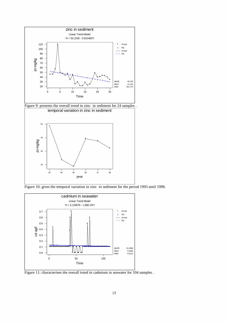
significance among stations [f(3,107)=0.444;NS]. Figure 9 presents the overall trend in zinc in sediment for 24

samples . The trend is dropping and that the Mean is 41.30 mg/kg with a minimum 21 mg/kg and maximum

110.07 mg/kg. Figure 10 gives the temporal variation in zinc in sediment for the period 1993 until 1998. The

lowest mean value 23.75 mg/kg is reported in 1995 and the maximum mean value 53.58 mg/kg is reported in

1993 . ANOVA test among years indicated non significance [f(5,23)= .069;NS]. Figure 11 characterises the overall

trend in cadmium in seawater for 104 samples . The trend is slightly declining and that the Mean is 0.12g /l with

a minimum 0.001g /l and maximum 0.71g /l. Figure 12 describes the temporal variation in cadmium in

seawater for the period 1993 until 1998. The lowest mean value 0.095g /l is reported in 1994 and the maximum

mean value 0.156g /l is reported in 1995 .ANOVA test among years indicated non significance [f(5,103)=

0.589;NS]. Figure 13 demonstrates the spatial variation in cadmium in seawater where the maximum mean

0.133g /l is registered in station 1 and that the lowest 0.108g /l is found in station 2. ANVOVA test showed

non-significance among stations [f(3,103)=0.855;NS]. Figure 14 shows the overall trend in cadmium in sediment

for 15 samples . The trend is falling and that the Mean is 0.09 mg/kg with a minimum 0.01 mg/kg and maximum

0.10 mg/kg. Figure 15 shows the temporal variation in cadmium in sediment for the period 1994 until 1998. The

lowest mean value 0.01 mg/kg is reported in 1996 and the means are equal for the other years. Figure 16 pictures

the overall trend in lead in seawater for 107 samples . The trend is slightly decreasing and that the Mean is

16.25g /l with a minimum 1.20 and maximum 87.60g /l. Figure 17 shows the temporal variation in lead in

seawater for the period 1993 until 1998. The lowest mean value 10.71g /l is reported in 1998, and the maximum

mean value 23.03g /l is reported in 1994 .ANOVA test among years indicated non significance [f(5,106)=

.004;NS]. Figure 18 demonstrates the spatial variation in lead in seawater where the maximum mean 20g /l is

registered in station 2 and that the lowest 13.05 g /l is found in station 4. ANVOVA test showed non-

significance among stations [f(3,106)=0.144;NS]. Figure 19 shows the overall trend in lead in sediment for 24

samples . The trend is abruptly decreasing and that the Mean is 48.75 mg/kg with a minimum 24 mg/kg and

maximum 76.95 mg/kg. Figure 20 shows the temporal variation in lead in sediment for the period 1993 until

1998. The lowest mean value 28 mg/kg is reported in 1995 and the maximum mean value 62.56 mg/kg is reported

in 1993 .ANOVA test among years Indicated significant differences[f(5,23) = 0.001] between 1993 and both 1994

and 1995(mean=42). Figure 21 depicts the overall trend in copper in seawater for 107 samples . The trend is

slightly descending and that the Mean is 3.04g /l with a minimum 0.10g /l and maximum 17.60g /l. Figure 22

illustrates the temporal variation in copper in seawater for the period 1993 until 1998. The lowest mean value

2.08g /l is reported in 1995,and the maximum mean value 3.63g /l is reported in 1993 . ANOVA test among

years indicated non significance [f(5,106)= 0.368;NS]. Figure 23 demonstrates the spatial variation in copper in

seawater where the maximum mean 3.52g /l is registered in station 4 and that the lowest 2.56g /l is found in

station 3. ANVOVA test showed non-significance among stations [f(3,106)=0.450;NS]. Figure 24 shows the

overall trend in copper in sediment for 24 samples . The trend is declining and that the Mean is 28.73 mg/kg

with a minimum 11 mg/kg and maximum 76.95 mg/kg. Figure 25 gives the temporal variation in copper in

sediment for the period 1993 until 1998. The lowest mean value 16.67 mg/kg is reported in 1994 and the

maximum mean value 37.45 mg/kg is reported in 1993 .ANOVA test among years indicated non significance

[f(5,23)= 0.173;NS].

Trace metals are a major anthropogenic contaminant of estuarine and coastal waters. Their inputs include urban

run-off, industrial effluents, mining operations and atmospheric depositions, and may be in particulate or dissolved

forms. Although many are essential biological elements, all have the potential to be toxic to organisms above

certain threshold concentrations, and for the protection of aquatic biota it is important that these limits not be

exceeded in aquatic environments (4).

Because most heavy metals tend to accumulate in sediments , their presence in the water column is usually the

result of recent inputs. Metal concentrations can vary significantly over short distances and as a function of tide.

Single measurements at a given site may indicate contamination.

Table 4 gives the ranges of seawater trace metals reported in this study that are determined to be Zn (1 - 124), Cd

(0 - 0.71) , Pb (1.20 - 87.6 ) , and Cu (0.10 - 17.60) µg /l . The State of the Environment Report did include

trace metals in the ROPME seawater environments for 3 states only, for Bahrain, Kuwait and Qatar . However, In

Australia, open ocean concentrations are estimated to be in the ranges for zinc (0.003-0.6), cadmium (0.0001-0.12

6

), lead(0.001-0.04), copper (0.03-0.4 µg /l), . In Houston Ship Channel, USA, the range values were determined

to be for zinc (30-280) , cadmium (0.3 - 3.3) , copper (0.3-25) and the lead average value is 0.68 µg /l.

Notwithstanding the fact that the reported values in this nearshore study (years 1993-1998) are below the Bahraini

effluent standard, nevertheless the lead level reported in this study is exceptionally high compared with other areas

and this may indicate that the area is under recent pollution loads and this will be dealt with in the sediment

section.

Table 5 shows the ranges of sediment trace metals reported in this study for the nearshore (1993 until 1998)

ranged for Zn (21-117.07), Cd (0.01 - 0.10), Pb (24.00 - 76.95), and Cu (11.00 - 76.95) mg/kg , and during

the period January 1983 until June 1991 ranged for Bahrain for Zn (2.34-3.79), Cd (0.011), Pb 0.64-24), and Cu

(1.16-17.6).

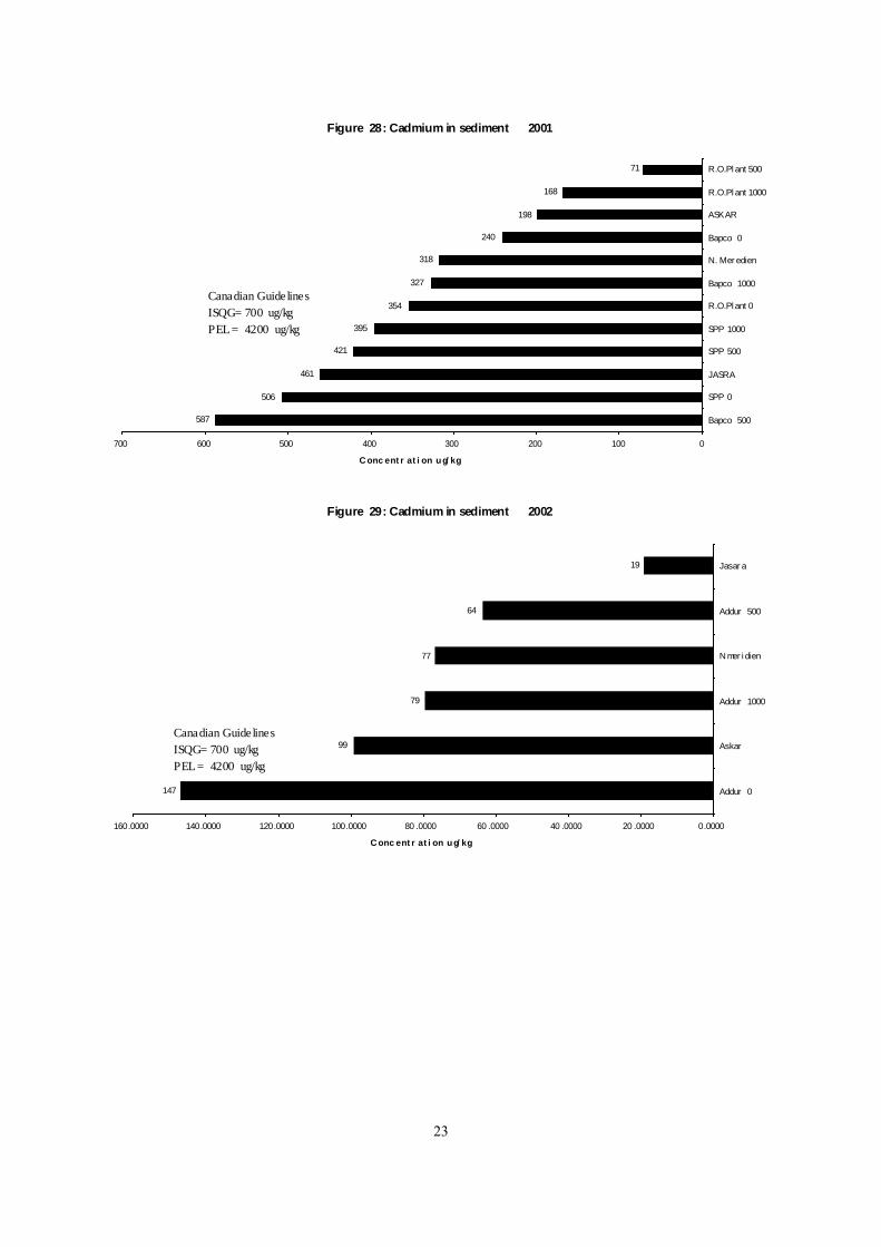
The pollution zonations studies for both years 2001 and 2002 for Zn(figures 26,27) ranged (12-451) and (3.6-29)

respectively, Cd(figures 28,29) ranged (71-587) and (19-147) respectively, Pb(figures 30,31) ranged (0-846) and

(0-12) respectively, Cu(figures 32,33) ranged (9.4-257) and (4-60) respectively, Ni (Figures 34,35) ranged (10-

181) and (4-60) ,respectively, for Cr(Figures 36,37) ranged (34-436) and (11-46) respectively, for Mn for year

2002 only(figure 38) ranged (23-64) ) Mg/kg.

Comparing these results with other parts in the ROPME region ranged for Zn( 0.7-410.3) Cd (0.01- 4.5), Pb (0.2 -

64.3), and Cu ( 1.3 - 142) mg/kg , and in the outside the region , in the Antarctic the mean values and the

standard errors of the mean are determined to be for the Zn( 42.3±10.4) Cd( 0.26±0.16), Pb (20.7±2.8) mg/kg. In

Semarang , Indonesia, the mean values Zn( 1257) Cd (< 0.03), Pb (2666), and Cu ( 448) mg/kg with the

reference values Zn (132.2), Pb (25.6), and Cu (40.7). DelValls et. al.(1998; (reference23)) evaluated heavy metal

sediment toxicity in littoral ecosystem using juveniles of fish. He suggested the following site-specific sediment

quality values; Cd 1.24, Pb 52.5, and Cu 71.2 mg/kg of dry sediment.

Trace metals sediments in industrial and developmental projects

The monitored industries included in the year 2001 were BAPCO ( representing oil refining industry) and both

Sitra Power Plant (SPP) and Reverse Osmosis Plant(ROP) , and in the year 2002 , the Addur Desalination

Plant(A.D.P).

Figure 26 shows the ranking comparison of the zinc in a transected sediments sampled in 2001. The range is 451-

12 mg/kg with the maximum in the vicinity of the SPP outfall. Both SPP and Bapco showed exceedances above

124 mg/kg of the Canadian guidelines. Figure 27 gives the zinc in the transected sediments sampled in 2002.

The range is 29-4 mg/kg and all values are within the accepted limit.

Figure 28 depicts the cadmium in the transected sediment in 2001.The range is 587-71 ug/kg. The highest value

was reported at 500m distance from Bapco discharge and the lowest was in the 500m distance from the ROP

outfall. Figure 29 gives the cadmium in transected sediment in 2002. The range is 147-19 ug/kg. The reported

values in both years are below the Canadian ISQG= 700 ug/kg.

Figure 30 demonstrates the spatial variation in the lead in the transected sediments sampled in 2001. The lowest

background is zero value in both Jasra(west coast of Bahrain) and north Meridien(north coast of Bahrain) areas.

The highest concentrations reported in the Bapco oil refinery area and extends to the Ras Abu Jarjour Reverse

Osmosis Plant maximum values 846-37 mg/kg were reported and they are above the 30.2 mg/kg of the Canadian

guidelines. Figure 31 shows the lead in the transected sediment in 2002. The range is 12-0 mg/kg. The highest

was in Askar and zero values were reported in Askar and north Meridien and addur zero and 500 metre distance

from the discharge points.

Figure 32 exhibits the spatial variation in copper in a transected sediments sampled in 2001. The range is 257- 9

mg/kg with the maximum in the vicinity of both the SPP and Bapco outfalls . SPP, Bapco and Ras Abu Jarjour

Reverse Osmosis Plant showed exceedances above 18.7 mg/kg of the Canadian guidelines, while the figure 33

shows the copper variation in the transected sediments sampled in 2002. The range is 60-4 mg/kg and that

exceedances confined only to addur 1000 metre distance from the discharge point, Askar and north Meridien.

7

Figure 34 characterises the overall comparison in nickel in transected sediments sampled in 2001 . The range is

180-10 mg/kg. Only SPP at zero and 500 metre distances from the discharge point showed exceedances above 35

mg/kg of the Dutch standard. Figure 35 gives the nickel in transected sediment in 2002. The range is 9-0 mg/kg.

The highest value was reported in north Meridien and the lowest value was in Jasra and the range is below the

Canadian guidelines value.

8

Figure 36 shows the spatial variation in chromium in transected sediment in 2001.The range is 436-34 mg/kg.

Exceedances above the 52.3 mg/kg of the Canadian guidelines were reported in SPP, north Meridien, Jasra and

Askar areas. However , north Meridien, Jasra and Askar areas showed no exceedances in 2002(figure 37).

Figure 38 gives the manganese in transected sediment in 2002. The range is 64-23 mg/kg . The highest value was

reported at zero distance from the ADP discharge point and the lowest was reported in Jasra.

As above mentioned in the seawater section, the lead level reported in this study is exceptionally high compared

with other areas in the ROPME Sea Area. This observation was further noted by Fowler et. al. (1993) who found

37.7 mg/kg Pb in rock scallop from Askar and the range between the period 1983-1986 was (1.2 - 7.2 mg/kg).

They suggested that pollution with Pb is relatively higher than values reported from other areas in the ROPME

Sea Area and could be attributed to the effluent discharges form industries located on the east coast of Bahrain . In

addition, They registered the mean lead concentration in the pearl oysters collected from Askar , the mean value

was 3.9 mg/kg compared with 2.1 mg/kg in 1986, and at Al Malikiya was 0.32 mg/kg compared with the range

for the period from 1983-1986 for Az Zallaq (0.8-2.4 mg/kg). However, Al-Sayed et. al. (1994; reference (12))

found that nearshore pearl oysters collected from Holiday Inn had lower concentration of lead compared with those

collected from offshore Bal Yaal site, (means 5.1, 7.6 mg/kg respectively). They maintained that illegal discharges

from ships are attributable for this elevated pollution. Fowler et. al. (1993) believed that during the Gulf war the

general trend of the concentrations of petroleum hydrocarbons related heavy metals found in sediment and biota

were not differed from that measured in earlier years in the same sites studied in the UAE, Oman and Bahrain.

Linden & Larsson (2002-Reference (13)) carried out the Bapco’s marine environmental assessment studies and

demonstrated that the concentrations of lead were 152 mg/kg, 447 mg/kg and 1010 mg/kg in years 2002, 1997 and

1992, respectively and claimed that the decrease of pollution is due to the company’s environmental improvements.

Bapco plan 2000-2009 includes control of Pb in refinery tank farm effluent(mid 1999-mid 2000), lead sulphide in

the refinery effluent system(mid 1999-2002) and Pb in refinery effluent(mid 2001-2004).

The elevated concentration of trace metals; zinc, copper, nickel, chromium, in vicinity of SPP is perhaps attributed

to the multi-flash stage operational system where it is expected that trace metals are coming off during clean up

the distillers. The marine sediment collected from the neighborhood of Reverse Osmosis Plant (Ras Abu Jarjour)

showed higher concentrations in lead and copper, where the marine sediment in immediate area of the oil

refinery exhibited higher levels of zinc, copper, lead and cadmium. The rejected water in SPP is about 70,000

tonnes per hour with a salinity range 50-55 ppm. ROP rejects 1050 cubic metre per hour with approximate

salinity of 36,000 milligram per litre. Bapco uses 1905 million cubic metre per month of cooling water, and this is

rejected after being mixed with pollutants during the cooling operations(National Environmental Strategy).

To conclude the presence of petroleum hydrocarbon and trace metals was confirmed in seawater and sediment in

the marine environment of the Kingdom of Bahrain . Results of nearshore monitoring during the period 1993-1998

indicated , in general, that concentration of the trace metals were higher in water columns than sediments and the

contrary was with the petroleum hydrocarbon. However , trace metals in transect sediments collected from the

coastal areas during the monitoring period 2001-2002 showed that Pb>Cd>Zn>Cu compared to the nearshore

sediments monitored during the period 1993-1998 that showed Zn>Pb=Cu>Cd. This study confirms that the lead

pollution is mainly concentrated in the vicinity of petroleum industry and that the Zinc and Cadmium in both the

Sitra Power Plant(SPP) and Bapco areas . SPP area showed higher pollution of Nickel, Copper and Chromium.

9

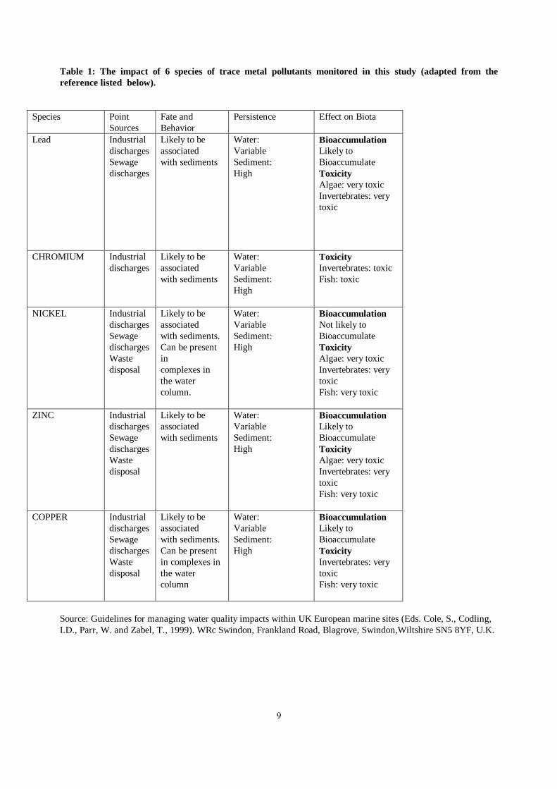
Table 1: The impact of 6 species of trace metal pollutants monitored in this study (adapted from the

reference listed below).

Species Point

Sources

Fate and

Behavior

Persistence Effect on Biota

Lead Industrial

discharges

Sewage

discharges

Likely to be

associated

with sediments

Water:

Variable

Sediment:

High

Bioaccumulation

Likely to

Bioaccumulate

Toxicity

Algae: very toxic

Invertebrates: very

toxic

CHROMIUM Industrial

discharges

Likely to be

associated

with sediments

Water:

Variable

Sediment:

High

Toxicity

Invertebrates: toxic

Fish: toxic

NICKEL Industrial

discharges

Sewage

discharges

Waste

disposal

Likely to be

associated

with sediments.

Can be present

in

complexes in

the water

column.

Water:

Variable

Sediment:

High

Bioaccumulation

Not likely to

Bioaccumulate

Toxicity

Algae: very toxic

Invertebrates: very

toxic

Fish: very toxic

ZINC Industrial

discharges

Sewage

discharges

Waste

disposal

Likely to be

associated

with sediments

Water:

Variable

Sediment:

High

Bioaccumulation

Likely to

Bioaccumulate

Toxicity

Algae: very toxic

Invertebrates: very

toxic

Fish: very toxic

COPPER Industrial

discharges

Sewage

discharges

Waste

disposal

Likely to be

associated

with sediments.

Can be present

in complexes in

the water

column

Water:

Variable

Sediment:

High

Bioaccumulation

Likely to

Bioaccumulate

Toxicity

Invertebrates: very

toxic

Fish: very toxic

Source: Guidelines for managing water quality impacts within UK European marine sites (Eds. Cole, S., Codling,

I.D., Parr, W. and Zabel, T., 1999). WRc Swindon, Frankland Road, Blagrove, Swindon,Wiltshire SN5 8YF, U.K.

01

Actual

Fits

Actual

Fits

100500

10

5

0

phc

ug/l

Time

Y t = 2.41068 + 2.16E-03*t

MSD:

MAD:

MAPE:

2.8306

1.2280

49.3910

petroleum hydrocarbons in seawater

Linear Trend M odel

Figure 1: illustrates the overall trend in petroleum hydrocarbons in seawater for 112 samples .

989796959493

3.0

2.5

2.0

1.5

year

phc u

g/l

temporal variation in phc in seawater

Figure 2 shows the temporal variation in petroleum hydrocarbons in seawater .

4321

3.1

2.6

2.1

station

phc u

g/l

spatial variation in phc in seawater

Figure 3 demonstrates the petroleum hydrocarbons spatial variation.

00

Table 2: Ranges of petroleum hydrocarbons in seawater in this study and other studies . Concentrations are

ranges in g/l.

Reference Concentration

This study 0.000 - 11.400

Bahrain(3) Means 22.4 - 43.3

ROPME(1) 0.10 - 16.8

Mediterranean( cited in 5) 1- 123

Australia(6) 0.1 - 22.6

Bahrain Std.(7) 8000( max. 15000)

Table 3 : Ranges of petroleum hydrocarbons in sediment reported in this study and other studies .

Concentrations are ranges in mg/kg.

Reference Concentration

This study 30.0 - 266.0

Bahrain before 1991(9) 20.3 - 103

Bahrain in 1991(8&9) 14.6 - 182

ROPME(4) 0.1-950

Black Sea(10) 2- 300

Cartagena Bay, Columbia(11) below 10 - 1415

02

Actual

Fits

Actual

Fits

2520151050

200

100

0

ph m

g/k

g

Time

Yt = 196.549 - 4.3234*t

MSD:

MAD:

MAPE:

2553.71

36.56

46.11

petroleum hydrocarbons in sedimentLinear Trend Model

Figure 4: gives the overall trend in petroleum hydrocarbons in sediment for 24 samples .

989796959493

185

175

165

155

145

135

125

115

105

year

ph m

g/k

g

temporal variation in pet.hcbns in sediment

Figure 5 shows the temporal variation in petroleum hydrocarbons in sediment for the period 1993 until 1998.

03

Table 4: Ranges of seawater trace metal concentrations in µg /l reported in this study and other studies with

their respective standards. Numbers in parentheses are the maximum allowable values, and the outer values

are means.

Reference Zn Cd Pb Cu

This study-

Nearshore(years 1993-

1998)

1.00-124.00 0.00-0.71 1.2-87.60 0.10-17.60

Bahrain(12) 0.03-11.25 0.03 - 0.38 0.03-0.23 0.03 - 0.38

Kuwait(4) <1 <10

Qatar(4) 0.9-130.3 Mean=0.8 0.1-15.6 Means=39.5-

20.1

Australia (14) 0.003-0.6 0.0001-0.12 0.001-0.4 0.03-0.4

USA (15) 30-280 0.3-3.3 mean = 0.68

Danube Delta(16) 0.04 - 1.54 0.30 - 2.30

North Aegean(16) 0.00 - 0.05 0.05 - 3.77

Bahrain Std (7) 2000 (5000) 10 (50) 200(1000) 200(500)

Int’nl Std (17) 2000 10 5000 500

Table 5: The ranges of marine sediment trace metals in mg/kg reported in this study and other areas. For

Canadian guidelines, the Interim marine sediment quality guidelines, ISQGs; dry weight, and numbers in

parentheses are probable effect levels, Pels; dry weight).

Reference Zn Cd Pb Cu

This study-Nearshore(years 1993-

1998)

21- 117.07 0.01- 0.10 24 - 76.95 11 - 76.95

This study-transect(year 2001) 12-451 71-587 0-846 9.4-257

This study-transect(year 2002) 3.6-29 19-147 0-12 4-60

Bahrain(9) 2.34-3.79 0.011-0.753 0.64-24 1.16-17.6

ROPME(4) 0.7 - 410.3 0.01 - 4.5 0.2 - 64.3 1.3 - 142

Arctic(18) 111 21 26

Antarctic(19) 42.3±10.4 0.26±0.16 20.7±2.8

Indonesia (20) 1257 < 0.03 2666 448

Togo (21) 60-632 2-44 22-176 22-184

Australia(14) 4 - 1150 0.1 - 13 0.5 - 520 0.2 - 180

Indonesia Ref. value(20) 132.2 25.6 40.7

Canadian Guidelines(22) 124 (271) 0.7 (4.2) 30.2 (112) 18.7 (108)

04

Actual

Fits

Actual

Fits

100500

100

50

0

zn u

g/l

Time

Yt = 16.9428 - 3.08E-02*t

MSD:

MAD:

MAPE:

242.789

9.483

116.366

zinc in seawaterLinear Trend Model

Figure 6: shows the overall trend in zinc in seawater for 108 samples .

989796959493

25

20

15

10

year

zn u

g/l

temporal variation in zinc in seawater

Figure 7: demonstrates the temporal variation in zinc in seawater for the period 1993 until 1998.

4321

18.6

17.6

16.6

15.6

14.6

13.6

12.6

11.6

station

zn u

g/l

spatial variation in zinc in seawater

Figure 8: exhibits the spatial variation in zinc in seawater.

05

Actual

Fits

Actual

Fits

2520151050

110

100

90

80

70

60

50

40

30

20

zn m

g/k

g

Time

Yt = 53.1035 - 0.922483*t

MSD:

MAD:

MAPE:

261.270

11.101

30.700

zinc in sedimentLinear Trend Model

Figure 9: presents the overall trend in zinc in sediment for 24 samples .

989796959493

55

45

35

25

year

zn m

g/k

g

temporal variation in zinc in sediment

Figure 10: gives the temporal variation in zinc in sediment for the period 1993 until 1998.

Actual

Fits

Actual

Fits

100500

0.7

0.6

0.5

0.4

0.3

0.2

0.1

0.0

cd u

g/l

Time

Yt = 0.129678 - 1.96E-04*t

MSD:

MAD:

MAPE:

0.0121

0.0482

21.9386

cadmium in seawaterLinear Trend Model

Figure 11: characterises the overall trend in cadmium in seawater for 104 samples .

06

989796959493

0.155

0.145

0.135

0.125

0.115

0.105

0.095

year

cd u

g/l

temporal variation in cadmium in seawater

Figure 12: describes the temporal variation in cadmium in seawater for the period 1993 until 1998.

4321

0.13

0.12

0.11

station

cd u

g/l

spatial variation in cadmium in seawater

Figure 13: demonstrates the spatial variation in cadmium in seawater.

Actual

Fits

Actual

Fits

2520151050

0.10

0.05

0.00

cd m

g/k

g

Time

Yt = 0.106817 - 1.08E-03*t

MSD:

MAD:

MAPE:

0.001

0.020

111.187

cadmium in sedimentLinear Trend Model

Figure 14: shows the overall trend in cadmium in sediment for 15 samples .

07

989796959493

0.10

0.09

0.08

0.07

0.06

0.05

0.04

0.03

0.02

0.01

year

cd m

g/k

g

temporal variation in cadmium in sediment

Figure 15: shows the temporal variation in cadmium in sediment for the period 1994 until 1998.

Actual

Fits

Actual

Fits

100500

90

80

70

60

50

40

30

20

10

0

pb u

g/l

Time

Yt = 16.7641 - 9.10E-03*t

MSD:

MAD:

MAPE:

124.411

6.506

67.931

lead in seawaterLinear Trend Model

Figure 16: pictures the overall trend in lead in seawater for 107 samples .

989796959493

22

17

12

year

pb u

g/l

temporal variation in lead in seawater

Figure 17: shows the temporal variation in lead in seawater for the period 1993 until 1998.

08

4321

20

19

18

17

16

15

14

13

station

pb u

g/l

spatial variation in lead in seawater

Figure 18: demonstrates the spatial variation in lead in seawater.

Actual

Fits

Actual

Fits

2520151050

80

70

60

50

40

30

20

pb m

g/k

g

Time

Yt = 65.9669 - 1.34609*t

MSD:

MAD:

MAPE:

109.772

8.223

21.571

lead in sedimentLinear Trend Model

Figure 19: shows the overall trend in lead in sediment for 24 samples .

989796959493

60

50

40

30

year

pb m

g/k

g

temporal variation in lead in sediment

Figure 20: shows the temporal variation in lead in sediment for the period 1993 until 1998.

09

Actual

Fits

Actual

Fits

100500

20

10

0

cu u

g/l

Time

Yt = 3.85674 - 1.44E-02*t

MSD:

MAD:

MAPE:

6.2936

1.4045

94.3312

copper in seawaterLinear Trend Model

Figure 21: depicts the overall trend in copper in seawater for 107 samples .

989796959493

3.7

3.2

2.7

2.2

year

cu u

g/l

temporal variation in copper in seawater

Figure 22: illustrates the temporal variation in copper in seawater for the period 1993 until 1998.

4321

3.5

3.4

3.3

3.2

3.1

3.0

2.9

2.8

2.7

2.6

station

cu u

g/l

spatial variation in copper in seawater

Figure 23: demonstrates the spatial variation in copper in seawater .

21

Actual

Fits

Actual

Fits

2520151050

80

70

60

50

40

30

20

10

cu m

g/k

g

Time

Yt = 35.0286 - 0.492169*t

MSD:

MAD:

MAPE:

213.254

10.520

39.861

copper in sedimentLinear Trend Model

Figure 24: shows the overall trend in copper in sediment for 24 samples .

989796959493

36

26

16

year

cu m

g/k

g

temporal variation in copper in sediment

Figure 25: gives the temporal variation in copper in sediment for the period 1993 until 1998.

20

22

Figure 26: Zinc in sediment 2001

451

133

120

97

59

47

41

40

38

31

24

12

050100150200250300350400450500

SPP 0

Bapco 500

Bapco 0

SPP 500

SPP 1000

Bapco 1000

R.O.Pl ant 500

JASRA

R.O.Pl ant 0

R.O.Pl ant 1000

ASKAR

N. Mer edien

C onc ent r at i on mg/ kg

Canadian Guidelines

ISQG= 124 mg/kg

PEL= 271 mg/kg

Figure 27: Zinc in sediment 2002

29

23

13

12

10

4

0.00005.000010.000015.000020 .000025.000030 .000035.0000

Addur 1000

Askar

N mer i dien

Jasar a

Addur 0

Addur 500

C onc ent r at i on mg/ kg

Canadian Guidelines

ISQG= 124 mg/kg

PEL= 271 mg/kg

23

Figure 28: Cadmium in sediment 2001

587

506

461

421

395

354

327

318

240

198

168

71

0100200300400500600700

Bapco 500

SPP 0

JASRA

SPP 500

SPP 1000

R.O.Pl ant 0

Bapco 1000

N. Mer edien

Bapco 0

ASKAR

R.O.Pl ant 1000

R.O.Pl ant 500

C onc ent r at i on ug/ kg

Canadian Guidelines

ISQG= 700 ug/kg

PEL= 4200 ug/kg

Figure 29: Cadmium in sediment 2002

147

99

79

77

64

19

0.000020 .000040 .000060 .000080 .0000100.0000120.0000140.0000160.0000

Addur 0

Askar

Addur 1000

N mer i dien

Addur 500

Jasar a

C onc ent r at i on ug/ kg

Canadian Guidelines

ISQG= 700 ug/kg

PEL= 4200 ug/kg

24

Figure 29: Cadmium in sediment 2002

147

99

79

77

64

19

0.000020 .000040 .000060 .000080 .0000100.0000120.0000140.0000160.0000

Addur 0

Askar

Addur 1000

N mer i dien

Addur 500

Jasar a

C onc ent r at i on ug/ kg

Canadian Guidelines

ISQG= 700 ug/kg

PEL= 4200 ug/kg

Figure 30: Lead in sediment 2001

846

577

108

53

37

25

18

17

13

1

0100200300400500600700800900

Bapco 500

Bapco 0

Bapco 1000

R.O.Plant 500

R.O.Plant 0

R.O.Plant 1000

SPP 500

SPP 0

ASKAR

SPP 1000

N. Meredien

JASRA

Concentration mg/kg

Canadian Guidelines

ISQG= 30.2 mg/kg

PEL= 112 mg/kg

0.0

0.0

25

Figure31: Lead in sediment 2002

12

2

0

0

0

0

02468101214

Askar

Addur 1000

N meridien

Jasara

Addur 0

Addur 500

Concentration mg/kg

Canadian Guidelines

ISQG= 30.2 mg/kg

PEL= 112 mg/kg

Figure 32: Copper in sediment 2001

257

93

83

70

42

41

22

21

19

15

15

9

050100150200250300

SPP 0

Bapco 500

Bapco 0

SPP 500

Bapco 1000

SPP 1000

R.O.Pl ant 0

R.O.Pl ant 500

JASRA

ASKAR

R.O.Pl ant 1000

N. Mer edien

C onc ent r at i on mg/ kg

Canadian Guidelines

ISQG= 18 .7 mg/kg

PEL= 108 mg/kg

26

Figure 33: Copper in sediment 2002

60

36

21

8

7

4

0.000010.000020 .000030 .000040 .000050.000060 .000070.0000

Addur 1000

Askar

N mer i dien

Addur 0

Jasar a

Addur 500

C onc ent r at i on mg/ kg

Canadian

Guidelines

ISQG= 18.7 mg/kg

PEL= 108 mg/kg

Figure 34: Nickel in sediment 2001

180

49

21

19

16

15

13

12

12

12

11

10

020406080100120140160180200

SPP 0

SPP 500

Bapco 500

SPP 1000

Bapco 1000

N. Meredien

Bapco 0

JASRA

R.O.Plant 0

R.O.Plant 500

R.O.Plant 1000

ASKAR

Concentration mg/kg

Dutch(VROM)

35 mg/kg

27

Figure 35: Nickel in sediment 2002

9

9

6

6

3

0

0.00001.00002.00003.00004.00005.00006.00007.00008.00009.000010.0000

N mer i dien

Addur 1000

Askar

Addur 0

Addur 500

Jasar a

C onc ent r at i on mg/ kg

Dutch (VROM)

35 mg/kg

Figure 36: Chromium in sediment 2001

436

113

100

76

57

55

49

42

42

40

35

34

050100150200250300350400450500

SPP 500

SPP 0

SPP 1000

N. Mer edien

JASRA

ASKAR

R.O.Pl ant 0

Bapco 0

R.O.Pl ant 500

Bapco 500

R.O.Pl ant 1000

Bapco 1000

C onc ent r at i on mg/ kg

Canadian Guidelines

ISQG= 52 .3 mg/kg

PEL= 160 mg/kg

28

Figure 37: Chromium in sediment 2002

46

34

25

24

23

11

0.00005.000010.000015.000020 .000025.000030 .000035.000040 .000045.000050.0000

Askar

N mer i dien

Addur 500

Addur 0

Addur 1000

Jasar a

C onc ent r at i on mg/ kg

Canadi an Guidel i nes

ISQG= 52.3 mg /kg

PEL= 160 mg /kg

Figure 38: Manganese in sediment 2002

64

50

44

41

41

23

0.000010.000020 .000030 .000040 .000050.000060 .000070.0000

Addur 0

Addur 1000

Askar

Addur 500

N mer i dien

Jasar a

C onc ent r at i on mg/ kg

29

References

1) EPC, Environmental Protection Committee (1995): Marine Monitoring Program Study of Physical and

Chemical Oceanography in Bahrain territorial waters. Environmental Protection Committee of the

Ministry of Housing , Municipalities and Environment and Directorate of Fisheries of the Ministry of

Works and Agriculture. Bahrain.

2) Manual of Oceanographic Observations and Pollution Analysis. Third Edition. Methods (MOOPAM)

(1999). Regional Organisation for the Protection of the Marine Environment (ROPME). Kuwait.

3) Madany, I. M., Jaffar , A. & Al-Shirbini , E. S. ( 1998): Variations in the concentrations of aromatic

petroleum hydrocarbons in Bahraini coastal waters during the period October 1993 to December 1995.

Environment International, 24:61-66.

4) Al-Majed N., Mohammadi, H. Al-Ghadban, A. and Al-Awadi, A.R. (2000): Regional Report of the State

of the Marine Environment. Regional Organization for the Protection of the Marine Environment

(ROPME), Kuwait, October 2000. ROPME Publication No. GC-10/001/1. Pp. 178.

5) Fowler, S.W.(1985): Coastal baseline Studies of Pollutants in Bahrain, United Arab Emirates and the

Sultanate of Oman. In: Proceedings of the Symposium on Regional Monitoring and Research

Programmes, Al-Ain, UAE. ROPME Publication.

6) Connell, D.W. (2001): Pollution: In the State of the Environment Report for Australia. Occurrence and

effects of petroleum hydrocarbons on Australia’s marine environment. Technical Annex 2, SOMER.

Environment Australia , Department of the Environment and Heritage.

7) Ministerial Order 10/1999 with respect to Environmental Standards (Air and Water). State of Bahrain

Gazette, 2378: 11-33, and revised by Ministerial Order 3/2001, Bahrain Gazette, 2507: 8-17.

8) Al-Wadae, A.E.J., and Raveendran, E.(1993): Determination of Petroleum hydrocarbons in Sediments ,

Fish and Air Following the Gulf Crises in 1991. Environmental Technology, 14:673-679.

9) Fowler, S.W., Readman, R.W., Oregioni, B., Villeneuve, J. -P., and McKay, K.(1993): Petroleum

Hydrocarbons and Trace Metals in Nearshore Gulf Sediments and Biota Before and After the 1991 War:

An Assessment of Temporal and Spatial trends. Marine Pollution Bulletin, 27:171-182.

10) Readman, J.W., Fillmann, G., Tolosa, I., Villeneuve, J. -P., Catinni, C., and Mee, L.D. (2002): Petroleum

and PAH contamination of the Black Sea. Marine Pollution Bulletin, 44:48-62.

11) Parga-Lozano, C.H., Marrugo-Gonzطlez, A.J., and Fernطndez-Maestre , R.(2002): Petroleum and PAH

contamination of the Black Sea. Marine Pollution Bulletin, 44:71-74.

12) Al-Sayed , H. A., Mahasneh, A.M., and Al-Saad, J.(1994): Variations of Trace Metal Concentrations in

Seawater and Pearl Oyster Pinctada radiata from Bahrain (Arabian Gulf) . Marine Pollution Bulletin,

28:370-374.

13) Linden, O. & Larsson, U. (2002): Marine Environment Assessment off the BAPCO Refinery. December,

2002. Bapco, Bahrain. Pp. 43.

14) Batley, G.E. (2001): Pollution: In the State of the Environment Report for Australia. Heavy metals and

tributyltin in Australian coastal and estuarine waters. Technical Annex 2, SOMER. Environment

Australia , Department of the Environment and Heritage.

15) Saleh, M.A. and Wilson, B.L. (1999): Analysis of Metals Pollutants in the Houston Ship Channel by

31

inductively Coupled Plasma/Mass Spectrometry. Ecotoxicology and Environmental Safety, 44:113-117.

16) Zeri, C., Voutsinou-Taliadouri, F., Romanov, A.S., Ovsjany, E.I., and Moriki, A. (2000): A

Comprehensive Approach of Dissolved Trace Element Exchange in Two Interconnected Basins: Black

Sea and Agean Sea. Marine Pollution Bulletin, 40:666-673.

17) El-Sharkawi, F.M. (1988 ): Environmental Health Aspects of Coastal Area Activities. In:

(ROPME/UNEP) proceedings of the ROPME Workshop on coastal area development. UNEP Regional

Seas Reports and Studies No. 90. UNEP, 1988 and ROPME Publication No. GC-5/006. Pp. 113-122.

18) Holemann, J.A. Scirmacher, M., Kassens, H., and Prange, A. (1999): Geochemistry of Surficial and Ice-

rafted Sediments from the Leptive sea (Siberia). Estuarine, Coastal and Shelf Science, 49:45-59.

19) Ciaralli, L., Giordano, R., Lombardi, G. , Beccaloni, E. , Sepe, A. ,and Costantini, S. (1998) : Antarctic

Marine Sediments: Distribution of Elements and Textural Characters , Microchemical Journal, 59:77-88.

20) Widianarko, B., Verweij, R. A., Van Gestel, C. A. M., and Van Straalen, N. M.(2000): Spatial

Distribution of Trace Metals in Sediments from Urban Streams of Semarang, Central Java, Indonesia .

Ecotoxicology and Environmental Safety, 46:95-100.

21) Gnandi, K. and Obschall, H. J.(1999): The pollution of marine sediments by trace elements in the coastal

region of Togo caused by dumping of cadmium-rich phosphorite tailing into the sea. Environmental

Geology, 38:13-24.

22) Canadian Council of Ministers of the Environment (2001). Canadian sediment quality guidelines for the

protection of aquatic life: Summary tables. Updated. In : Canadian environmental quality guidelines,

1999, Canadian Council of Ministers of the Environment, Winnipeg. Publication No. 1299; ISBN 1-

896997-34-1.

23) DelValls, T. A. , Blasco, J., Sarasquete, M. C. , Forja, J. M. , and Gomez-Parra, A. (1998): Evaluation of

Heavy Metal Sediment Toxicity in Littoral Ecosystems Using Juveniles of the Fish Sparus aurata.

Ecotoxicology and Environmental Safety, 41:157-167.