LARS Print 030772

<*F-

V

C M £** gon gs» „ »A S E F I L E

Minimum DistanceClassification inRemote Sensing

byA.G.Wacker andJD. A. Landgrebe

The Laboratory for Applications of Remote SensingPurdue University ;H

Lafayette, Indiana !

https://ntrs.nasa.gov/search.jsp?R=19730007762 2019-03-24T04:42:00+00:00Z

L.A.R.S. Print #030772

MINIMUM DISTANCE CLASSIFICATIONIN REMOTE SENSING*

by

A. G. Wacker and D. A. Landgrebe

SUMMARY

The utilization of minimum dis-tance classification methods in remotesensing problems, such as cropspecies identification, is considered.Minimum distance classifiers belong toa family of classifiers referred to assample classifiers. In such classi-fiers the items that are classifiedare groups of measurement vectors(e.g. all measurement vectors from anagricultural field), rather than in-dividual vectors as in more conven-tional vector classifiers.

Specifically in minimum distanceclassification a sample (i.e. group ofvectors) is classified into the classwhose known or estimated distributionmost closely resembles the estimateddistribution of the sample to beclassified. The measure of resemblanceis a distance measure in the space ofdistribution functions.

The literature concerning bothminimum distance classification pro-blems and distance measures is review-ed. Minimum distance classificationproblems are then categorized on the

*This paper was presented at the FirstCanadian Symposium for Remote Sensing,February 7-9, 1972, Ottawa, Canada. Dr.Wacker is Associate Professor, Depart -ment of Electrical Engineering,University of Saskatchewan, Sakatoon,Saskatchewan. Dr. Landgrebe is Director,Laboratory for Applications of RemoteSensing and Professor, Department ofElectrical Engineering, Purdue Univer-sity, West Lafayette, Indiana. The workdescribed was sponsored by NASA underGrant No. NGL 15-005-112.

basis of the assumption made regard-ing the underlying class distribution.

Experimental results are presentedfor several examples. The objective ofthese examples is to: (a) compare thesample classification accuracy (%samples correct) of a minimum distanceclassifier, with the vector classifi-cation accuracy (% vector correct) ofa. maximum likelihood classifier; (b)compare the sample classificationaccuracy of a parametric with a non-parametric minimum distance classifier.For (a), the minimum distance classi-fier performance is typically 5% to10/2 better than the performance of themaximum likelihood classifier. For(b), the performance of the nonparame-tric classifier is only slightlybetter than the parametric version.The improvement is so slight that theadditional complexity and slower speedmake the nonparametric classifier un-attractive in comparison with the para-metric version. In fact disparitiesbetween training and test results sug-gest that training methods are of muchgreater importance than whether theimplementation is parametric or non-parametric.

INTRODUCTION

A fairly common objective ofremote sensing in connection with earthresources is to attempt to establishthe type of ground cover on the basisof the observed spectral radiance.The examination of systems capable ofachieving this objective shows that a

certain duality of system types exists.Landgre~be refers to the two types asimage-oriented systems and numerically-oriented systems. The duality existsprimarily for historical reasons as aconsequence of the independent develop-ment of photographically oriented andcomputer oriented technology. Theprimary distinction between the twosystem types is that in image orientedsystems a visual image is an essentialpart of the analysis scheme while innumerically oriented systems thevisual image plays a secondary role.In Fig. 1 the location of the "FormImage" block in relation to the"Analysis" block characterizes the twosystem types.

In numerically oriented remotesensing systems it is frequently pos-sible to design the data collectionsystem in such a manner that classifi-cation becomes a problem in patternrecognition. This situation prevailsif one attempts to study earth re-sources through the utilization ofmultispectral data-images. The termmultispectral image (i.e. without themodifier data) is used to refer to oneor more spectrally different superim-posed pictorial images of a scene.The modifier data is added to indicatethat images are stored as numericalarrays as opposed to visual images.

To obtain a multispectral data-image of a scene, the scene in questionis partitioned on a rectangular gridinto small cells (pixels) and theradiance from each pixel for each wave-length band of interest is measuredand stored. The set of measurementsfor a pixel constitutes the measure-ment vector for that pixel. A multi-spectral data-image for a scene issimply the complete collection of allmeasurement vectors for the image.The spatial coordinates (i.e. row andcolumn number) of each pixel are ofcourse also recorded to uniquelyidentify each measurement vector.Fig. 2 depicts the situation.

The methods used to generatemultispectral data images can conven-

iently be divided into two categories.In the first category, film is used torecord the image. The film is subse-quently scanned and digitized to pro-duce a. data-image. The multispectralproperty is obtained either by scanningseveral images photographed throughdifferent spectral windows, and over-laying the data; or by utilizing colorfilm and separating the spectral com-ponents during the scanning procedure.In the second category the image isgenerated electrically and stored inan electrically compatible form,usually on magnetic tape as either ananalog or digital signal. The electri-cal signal to be stored can be gener-ated by a number of different systems*,the multispectral scanner and returnbeam vidicon probably qualify as thetwo most common examples. For thescanner the multispectral property isobtained by filtering of the spectralsignal collected through a single aper-ture prior to recording, or by thesuperposition of several unispectralimages collected through different ap-ertures .

As already stated, pattern recog-nition techniques can serve as thebasis for affecting classification ofmultispectral data-images. Much ofpattern recognition theory is formu-lated in terms of multidimensionalspaces with the dimensionality of thespace equal to the dimensionality ofthe vectors to be classified. Thisvector dimensionality is, of course,determined by the number of attributesor properties of each pixel to be con-sidered in the classification (e.g.number of spectral bands). Classify-ing a multispectral data-image byclassifying the observation vectorsfrom such an image on a pixel-by-pixelbasis falls naturally into this commonpattern recognition framework. In con-trast to this vector-by-vector approachthere are classification schemes whichcollectively will be referred to as"sample classification schemes". Insuch schemes all vectors to be classi-fied are first segregated into groups(i.e. samples) such that all the vec-tors in a group belong to the same

class. The whole group of vectors isthen classified simultaneously. Theminimum distance method considered isone such classification scheme.

In utilizing sample classificationschemes two distinct problems can beidentified. The first is concernedwith partitioning the measurement vec-tors into homogeneous groups, whilethe second is concerned with theclassification of these groups. Ex-cept for the comments in the nextparagraph consideration is restrictedto the second problem.

It frequently occurs for multi-spectral data-images that many of theadjacent measurement cells belong tothe same class. For example in an ag-ricultural scene each physical fieldtypically contains many pixels. Infact it is precisely this conditionthat prompts the investigation of sam-ple classification schemes. In suchsituations the physical field bounda-ries serve to define suitable samplesfor problems like crop species identi-fication, and it is in this contextthat sample classifiers might also bereferred to as per-field classifiers.It is apparent that for the situationjust described one method of automat-ically defining samples is to devise ascheme that automatically locates phy-sical field boundaries in the multi-spectral data-imagery ' . For theminimum distance classification resultspresented later, physical field bound-aries will actually be used to definethe samples, but the field boundariesare located manually rather than auto-matically. A second and perhaps morepromising approach to the problem ofdefining samples is via observationspace clustering. In this approachvectors from an arbitrary area areclustered in the observation space, andall the vectors assigned to the samecluster constitute a sample irrespec-tive of their location in the arbitrarychoosen area. In this case the termfields no longer seems appropriateand consequently the term sample class-ifier is preferred over the term per-field classifier.

It is apparent that sample class-ification schemes cannot be used in allsituations where a vector-by-vectorapproach is possible. A basic require-ment is that the data to be classifiedcan either be segregated into homogen-eous samples or occur naturally inthis form. Where the minimum distancescheme can be applied it intuitivelyhas several potential advantages overa vector-by-vector classifier; inparticular it is potentially fasterand more accurate.

It seems logical that providedthe time required to automatically de-fine the samples is not too great, thensample classifiers should be fasterthan a vector-by-vector classifier.This is of considerable importance inutilizing a numerically oriented remotesensing system to survey earth re-sources because a characteristic of 'such surveys is the tremendous volumeof data involved. One would also an-ticipate that the vector classificationaccuracy (% vectors correctly classi-fied) for vector-by-vector classifiers'would be lower than the sample classi-fication accuracy (% samples correctlyclassified) for sample classifiers.The reason for this is that in sampleclassifiers all the information con-veyed by a group of vectors is used toestablish the classification of eachvector, whereas in vector-by-vectorclassifiers each vector is treatedseparately without reference to anyother vector. In a sense sample class-ifiers utilize spatial information be-cause vectors are classified as groups,which naturally have some spatial ex-tent. No spatial information is usedin vector-by-vector classifiers, con-sequently, sample classifiers shouldperform better since spatial informa-tion is certainly of some value.

MINIMUM DISTANCE CLASSIFICATION

Problem Formulation

In a certain sense minimum dis-tance classification resembles what isprobably the oldest and simplest ap-

proach to pattern recognition , namely"template matching" . In templatematching a template is stored for eachclass or pattern to be recognized (e.g.letters of the alphabet) and an un-known pattern (e.g. an unknown letter)is then classified into the patternclass whose template best fits the un-known pattern on the basis of somepreviously defined similarity measure.In minimum distance classification thetemplates and unknown patterns are dis-tribution functions and the measure ofsimilarity used is a distance measure"between distribution functions. Thusan unknown distribution is classifiedinto the class whose distribution func-tion is nearest to the unknown distri-bution ir terms of some predetermineddistance measure. In practice the dis-tribution functions involved are usu-ally not known , nor can they be ob-served directly. Rather a set of ran-dom measurement vectors from each dis-tribution of interest is observed andclassification is based on estimatedrather than actual distributions .

It is necessary to define moreprecisely what constitutes a suitabledistance for minimum distance classi-fication. Mathematically the terms"distance" and metric are used inter-changeably. For our purpose it is con-venient to distinguish between the twoterms. In essence all that is requiredfor a well-defined minimum distanceclassification rule is a measure ofsimilarity between distribution func-tions which need not necessarily pos-sess all the properties of a metric.The term distance refers to any suit-able similarity measure; the termmetric is used in the normal mathemat-ical sense. More specifically a metricon a set S is a real valued function6(.,.) defined on S X S (X indicatescartesian product) such that for arbi-trary F,G,H in S

(a)

(c)(d)

(2)

6(F,G) >. 0 15(F,F) =0 2If 6(F,G) = 0 then F = G 36(F,G) = S(G,F) U6(F,G) + 6(G,H) >. 6(F,H) 5

A distance, as used herein, is definedto be a real valued function d(.,.) onS X S such that for arbitrary F,G,H in Sat least metric properties a,b(l) andusually b(2) and (c) hold. For theoreti-cal proofs it is in fact often desire-able to require that d be a true metricwhile in practical application such arestriction is usually not necessary.

Not only are distances betweenindividual distribution functions ofinterest but since each class couldconceivably be represented by a set ofdistribution functions the distancebetween sets of distributions is alsoof interest. Definition 1 defines thedistance between sets of distributions.

Definition 1 - Let the distanced(F,G) be defined for all F,G, in A,where A is an arbitrary set of cdf'sof interest. If Aj_ and A2 are non-empty subsets of A then the distanced(A , A2) between the sets AI and A2is defined as

d(A1> A2) = Inf d(F,G)

Note that Definition 1 applies tofinite and infinite sets of distribu-tion functions. Of course, if the setsare finite then taking the infimum isequivalent to taking the minimum.

Futhermore , if each set consistsonly of a single distribution functionthen the distance between the sets isprecisely the distance between thedistribution functions. The distancebetween a distribution function and aset of distribution functions is alsoincluded as a special case. It isnecessary to make some comments aboutthe usage of the notation d(F,G) .Some of the distance measures consid-ered are expressed in terms of prob-ability density functions (pdf *s)rather than cumulative distributionfunctions (cdf's). The conventionadopted is that the notation d(F,G) isstill used and referred to as the dis-

tance between cdf s, even though thedistance is expressed in terms of thedensities of F and G (i.e. in terms off and g) .

The minimum distance classifica-tion scheme can now be formally defin-ed. It is convenient to use a decisiontheoretic framework for this purpose.In general to specify a problem in thisframework it is necessary to specify:

(a) Z - the sample space of the observ-ed random variable .

(b) £2 - the set of states of nature;that is, the set of possible cdf's ofthe random variable. If the function-al form of the cdf is known, then Qcan be identified with the parameterspace.

3g

(c) A - the action space; that is theset of actions or decisions availableto the statistician.

£d) L (a,F) - loss function defined onAXQ which measures the loss incurred ifFcfi is the. true state of nature andaction aeA is the action taken.

The general formulation of theminimum distance problem in this frame-work follows :

(a) Z = E (q-dimensional Euclideanspace )

(b) n = [ f i , n , . . . . , f i ] vhereis the set of possible distributionfunctions for the ith class, i = 1, 2,• • • y it •

(c) A = [alt &2» ..., a.] where a^ isthe decision to decide the random sam-ple' to be classified belongs to theith class, i = 1, 2, ...,k.

(d) L(a,F) = 0 ifwas taken

L(a,F) = 1 otherwise.

and action

A decision rule is a function de-fined on Z and taking values in A. Theminimum distance decision rule is givenby definition 2.

Definition 2 - Let Y be the vectorof all sample observations. The mini-mum distance decision rule DMD'•&»•* isDMD(Y_) = a± (I.e., decide the randomsample to be classified belongs toclass i) in case

d(FH, A(i)

J = N, A(J>)Where A is the set of cdf's select-ed to represent the ith class and %is a sample-based estimate 6f the cdfof the random sample classified.

Several items in definition 2 re-quire clarification. The vector Y in-cludes not only the random sample tobe classified, but also any other ob-servations used in the classificationprocedure. For example, if trainingsamples are used for each class, theseare included in Y. The sets A^i) alsorequire comment. A^' may be the setof all possible.distributions forclass i (i.e. A^; = fi(i') or it maybe a subset of n'i) or the sample-based estimates of a set cdf's select-ed to represent class i. Finally theterm sample-based estimate is used torefer to any estimate of a cumulativedistribution function or its corre-sponding density which is based on arandom sample from the distribution inquestion. A number of suitable esti-mators exist^ and the present formula-tion does not restrict the type ofestimator. Later attention will befocused on distance measures based ondensities. In the parametric case thedensities will be estimated by esti-mating the parameters describing thedensities (parametrically estimatedpdf's). In the nonparametric case den-sity estimates will be based on histo-grams (density histogram estimation).To obtain a density histogram estimateof a pdf the observation space ispartitioned into square bins and theprobability.density estimate in anybin is the percent of vectors used toestimate the density which fall in thebin.

A number of special cases of the

vPabove formulation are noty considered.These special cases are basically aconsequence of making different as-sumptions regarding J2, and A = [A 1',A<2), ..., A k)]. In Type I problemsthe sets of distribution functions re-presenting the classes are assumed tobe known sets. Actually, this pro-blem is not of great interest from apractical point of view, since classdistributions are not normally known,but it is interesting from a theoreti-cal point of view because of its rela-tive simplicity.

Type I - The flcdf's

(i),

Case (a) The sets

Case (b)

s are known sets of

are infinite and

e sets, p) = n(i)

are finite and

Case (c) The setscdf/class) and A

Type II problems differ from TypeI problems in that the possible dis-tribution functions for each class areknown to be q-variate distributionsbut are otherwise unknown. Consequent-ly, all distributions used in the mini-mum distance decision rule must be est-imated. Since in practice only afinite number of estimated distribu-tions can be utilized this factor mustbe considered in formulating the pro-blem. If the sets of states of nature(e.g. the flUJ's) are infinite theinfinite sets must somehow be replacedby a representative finite set. Asimilar attitude must be adopted if itis known a_ priori that the sets ft(i)are finite but it is not known precise-ly how many distribution functions eachn\i) contains (e.g. how many subclassesof wheat are there?); or even if theprecise number is known, it may not beknown how to obtain a random samplefor each distribution function (i.e.how are samples representing differentsubclasses of wheat selected?). Final-ly, in the finite case, even if a ran-dom sample for each distribution func-tion of interest can be obtained,

their number may be so large that forpractical reasons it may be desireableto use a smaller number of representa-tive distributions. Thus , the needarises for a method to select a repre-sentative set of distribution func-tions from a larger (possibly infinite)set. To do this assign a distributionH*U) to Wi), i - 1, 2, ..., k. Thatis the events to which probabilitymass is assigned by H*'*' are sets ofdistributions in ft'1). To select arandom set of cdf's from J^1' (i.e. toselect a random set of training sam-ples for the ith class) is now equiv-alent to selecting a random samplefrom H*^1).

The above formulation is rathercomplicated in that a distribution overa space of functions is involved. Thiscomplexity can be avoided by restrict-ing consideration to a parametric fam-ily characterized by s real parameters.Making the logical assumption that aone to one correspondence exists be-tween cdf's in f 1' and points in theparameter space e(i)(=Es), it is ap-parent that assigning a distributionH*(i) to n( ' is equivalent to assign-ing some other distribution H^i' tothe parameter space e'i'. Consequent-ly, in the parametric case rather thandeal with H*'i', which is a cdf on aset of distribution function, only H(i)which is a cdf in Es need be consider-ed.

It is perhaps, worthwhile to re-state the above ideas in terms of mul-tispectral data-imagery from an agri-cultural scene before stating them ina more formal manner. In the interestof simplicity and since it is the caseof primary interest assume that thetrue q-dimensional distribution of the' radiance measurements from each fieldbelong to the same parametric familywhich can be characterized in the para-metric space Es. This family may havea finite or infinite number of members(i.e. subclasses). Further assume thatall the fields in a class (e.g. wheat)can be described by a suitable distri-bution H'*' over the parameter space.A set of training fields for each class

is selected at random. Because of ourformulation this is equivalent to se-lecting a random sample from the para-meter space according to the assumeddistribution over the parameter spacefor that class (i.e. H 1'). For eachof the randomly selected trainingfields the radiance measurements areused to get an estimated cdf • for thatfield. In this way estimated cdf'sfor a representative set of trainingfields are obtained for each class.An unknown field is then assigned tothe class that has a training fieldwhose estimated cdf is nearest to theestimated cdf of the unknown field.Since the problem as stated is parame-tric, one would normally, though notnecessarily, use parametrically esti-mated cdf's .

Type II problems in which theo,(i)'s are unknown are now formallydescribed. While prime interest iscentered in the case where fi is a para-metric family this restriction is notimposed in stating the problem. Thedescription of Type II problems is com-plicated by the fact that, the descrip-tion of the sets A'1' is rather in-volved.

Type II - Theof cdf's

are Unknown Sets

Case (a) - The sets fi(i) are infinitein number and h^' = P,M.(i). The setsJ2M-^' are now described. First a setof population cdf's corresponding to arepresentative set of Mi trainingfields for class i, i = 1, 2, ..., kis selected. Let %. 'i' be this setfor the ith class. """That is__nM. U) ,-i-s.a random sample of size MI for~ &*»*•'.A sample-based cdf is then obtainedfor each cdf in flMi^' for i B 1» 2,..., k. The resultant set of sample-based estimated cdf's is OM *). For

the case where parametrically estimat-ed cdf's are used QM^ *' can also beconsidered to be a random sample ofsize Mi in the parameter space accord-ing to a distribution H '.

Case (b) - The sets fi(i) are finite andA(i) = o(i) or A^) = P,Mi

(i) "(i)- If

the Jr1^ are finite sets (i.e. finitenumber of subclasses) then it is de-sireable to let A^1' = , wherefi is the set of sample-based esti-mated cdf's for the ith class. Incases where the resultant number ofsubclasses is impractically large and/or only a random set of M^ trainingfields is available it is necessary tolet A^1) = %. (iJcftU) and proceed asin case (a) . .

Case (c) - The set ficdf per class) and A

Distance Measures

= F(I) (Single= F]\j(i).

The importance in statistics ofdistances between cdf's has, of course,long been recognized; according toSamuel and Bachi" their use appears.to fall into two broad categories .

(a) Used for descriptive purposes.For example, as an indicator to quanti-tatively specify how near a given dis-tribution is to a normal distribution.

(b) Use in hypothesis testing, whichis, of course, a special case of de-cision theory.

There is a tendency for distancefunctions sufficiently sensitive todetect minor differences in distribu-tion functions (i.e. category (a) use)to be somewhat involved functions ofthe observations, with the result thattheir use as test statistics in hypoth-esis testing has been limited becauseof the complicated distribution theory.On the other hand, distance functionswhose theory is simple enough to bereadily used as test statistics oftendo not distinguish distribution func-tions sufficiently well. Since inminimum distance classification inter-est is naturally centered on good dis-crimination between distribution func-tions, therefore distance functionsthat fall into category (b) are nor-

8

mally used. Since the appropriatedistribution theory for hypothesistesting is then in general not knownit is impossible to theoreticallycompute probability of error, but itmay be possible to establish reason-ably tight upper bounds. The approxi-mate probability of error can ofcourse be determined experimentally.

The literature abounds with refer-ences to distance measures and no at-tempt will be made to give a completebibliography. A representative sampleof distance measures is given in Table1. This Table includes the most widelyused distance measures because of theirobvious importance, as veil as more ob-scure distance measures whose applica-tion to the present problem appears•reasonable. In addition a few miscel-laneous distance measures have beenincluded to give an indication of thevariety of distances that have beensuggested. The distances included inthis Table are: Cramer-Von MisesT,8,9AO, Kolmogorpv-Smirnov11'12^,^Divergencel3.l4.15 Bhattacharyyal5»l6,Jeffreys-Matusita-^»!** >171 KolmogorovVariationall5.18,19, Kullback-Leibler15»20, Swain-Fu21, Mahalanobis22>23,Samuels Bachi°, and Kiefer-Wolowitz2^.The references cited are by no meanscomprehensive. In selecting the re-ferences the attempt has been made tocite only the original source inaddition to survey papers. The paperby Darling?, Sahlerl° and to a cer-tain extent Kalaithl5 fall in thislatter category.

Most of the references cited areconcerned only with the univariateforms of the distance measure. Withthe exception of the Samuels-Bachidistance, the extention to the multi-variate forms is quite natural. Sinceit is the multivariate forms that areof interest, these, rather than themore common univariate forms, are givenin Table 1. For the Samuels-Bachi dis-tance multivariate forms other thanthe one presented may be possible.

Table 1 also contains informationregarding the metric properties of the

distance measures when used in conjunc-tion with three families of distribu-tion functions. The families consider-ed are: C, the family of q-variateabsolutely continuous distributionfunctions; MVN, the family of q-variatenormal distribution functions; andMVNj;, the family of q-variate normaldistribution functions with equal co-variance matrices. Since MVN and MVNj;are subsets of C it is, of course,true that a metric -in C is also ametric in MVN and MVNj;. A metric inMVNj need not, however, be a metric inMVN or C.

Because of the importance of themultivariate normal distribution, ex-pressions for the distance between twosuch distributions are given in Table2 for each of the distances measuredin Table 1 in those instances where theexpressions are known.

The distances listed in Table 1are discussed in the references citedand no attempt will be made to discussthem except for some general commentspertaining to their use in minimumdistance classification.

Since a large variety of distancemeasures is available, the problem nat-urally arises as to which distance mea-sure to use in a given problem. Unfor-tunately, no complete answer to thisquestion is presently available, butsome general comments are possible.The distribution-free properties* thatmake the Cramer-Von Mises andKolmogorov-Smirnov distances so popu-lar in the univariate case do not applyin the multivariate case. Since it isthe multivariate case that is of inter-est these distances lose their specialappeal. Intuitively a distance likethe Kolmogorov-Smirnov distance doesnot appear to be as good a distance

* In the univariate case the distribu-tion of the Kolmogorov-Smirnov andthe Cramer-Von Mises distances betweentwo estimated distribution functions isindependent of the underlying distri-butions being estimated, providedappropriate estimators are used.

Table 1

Multivariate Forms of Distance Measures andTheir Metric Properties

Metric inName Form C MV.N MVNr

1.

Cramer-Von Mises W = {/"(OU) - F(x))2dx)2 lea Yes tea

JColjnogorov-Smirnov K » Sup \G(x) - F(x_) | lea Yes lea

Divergence J = /"^(~-'(f (x)-g(x) )da Mo «o les

Bhattacharyya Distance B « -Ln/~(r(x_)g(x_)) dx No So Yes

Distance~MatU8ita M " t/"'" ? " /f (x.) )2dx)2 Yes Yes Yes

n? !?°I°V Varlati°nal K(P) • riP.B(x)-P,f(«)l*L Yes Yes Yes

Kullback-Leibler f- , . ., . .., v. I*, • J kit /**.) f(x;dx No No YesNumbers fg ' '-'~\' *— — •

Swain-Fu Distance . T • „ .I6 No No Yes

IE,-!' I2 (q+2) 2here D = ( . JT ~ 11 rj-)

1 -g f g

i

Mahalanobls Distance A • {(u -v. )tl~i(i>-IL,'> )2 "es

i

Samuels-Bach! Distance U = (/1[F"1(a)-o":L(a) Jdo)2 No No No0

— iwhere F (a) » Inf{c|Q nQ 0}

qand (J » (x| I x <c), Q » (x|F(x)>a)

1=1 1 °

|e"lx'dx . Yes Yes Yes

Notation

(1) F, G are multlvariate cdf's with densities f, g; means u_, p ; covariances lf, Z ;and prior probabilities p , p . "^ 8

(2) /"() d£ designates a multivariate integral.

(3) For Mahalanobis distance F and G are normal with means p_^ and \i and have commoncovariance I. ~

CO || designates the absolute value or vector norm.

(5) t designates the transpose.

10

Table 2

Distances Between Two Multivariate Normal cdf's

Name

Divergence

BhattacharyyaDistance

Jeffreys-MatusitaDistance

Distance

J =

-1 x det(|[Zf+Z ])

{det(Z )det(Z

g

g

Z -Z

Kullback-LeiblerNumbers

8wain-Fu Distance

MahalanobisDistance

fg

det(Zf) 1

g

where D = {-g

{(iL.-V v ' vy

Notation

(1) t means transpose

(2) det means determinant

(3) tr means trace

The normal distributions involved have means and u and covariance matrices Z and Zu

11

measure as those involving integrationover the whole space. It is also moredifficult to compute in parametricsituations then some of the integralrelations. The Samuels-Bachi distancesuffers from a similar computationaldisadvantage.

The Divergence, Bhattacharyya dis-tance, Jeffreys-Matusita distance,Kolmogorov variational distance andKullback-Leibler numbers all belong toa class of distance measures which canbe written as the expected value of aconvex function of the likelihoodratio*. In fact Ali and Silvey •* haveshown that the expected value of anyconvex function of the likelihood ratiohas properties that might reasonably bedemanded of a distance measure. Inaddition Wacker^ has shown that in fea-ture selection such distance measureshave a weak relationship to the prob-ability of error. Kalaithl5 proved .thesame relationship for Divergence andthe Bhattacharyya distance. Since theclass of distance measures under dis-cussion is based on pdf's there isprobably a tendency for these distancesto reflect differences in pdf's ratherthan cdf's.

Of the distances based on likeli-hood ratios the Bhattacharyya distanceseems to have been gaining in favor.The prime reason for this is apparentlythe close relation between probabilityof error and Bhattacharyya distance,as well as the relative ease of com-puting Bhattacharyya distance in theo-retical problems. Other properties ofthe Bhattacharyya distance which en-hance its prestige as a distance mea-sure have been pointed out by Lainiotis

and Stein^T. A property of consid-erable theoretical utility is the closerelation between the Bhattacharyya dis-tance B, the Jeffreys-Matusity distanceM and the affinity p namely

andp(F,G) = C»(f(x)g(x' 10

M = 2(l-p)l/2 = 2(l-e-B)l/2WhereB = -Lnp

8

9

* The likelihood ratio of densitiesf(x) and g(x) is f(x)/g(x).

Because of the above relationshipsminimum distance classifications madeon the basis of the Bhattacharyya dis-tance, Jeffreys-Matusita distance oraffinity all yield identical results,and consequently have identical proba-bility of error.

The Jeffreys-Matusita distance is,however, a metric in a much largerclass of distributions (see Table l).This means that theoretical derivationsregarding probability of error can bemade using the metric properties ofthe Jeffreys-Matusita distance in thislarger class, and the results are ap-plicable if classification is effectedusing Bhattacharyya distance or affin-ity as well. This property has beenused extensively by Matusita.

While no strong preference forany distance measure can presently bedemonstrated the theoretical propertiesof the Bhattacharyya distance suggeststhat it might be a reasonable choiceand the experimental results presentedlater are based on this distance mea-sure.

Minimum Distance Classification AndProbability of Error

Considerable literature exists onthe minimum distance method withMatusita^°~35 and Wolfowitz3"~39 beingthe chief contributors. Wolfowitz'swork is concerned primarily with esti-mation while much of Matusita's workdeals with the decision problem. Con-tributions have also been made by Gupta1+0, Cacoullous^1'1*2, Sirvastava^S andHoeffding and Wolfowitz1*1*.

In considering minimum distancedecision rules a common requirement isto insist that by using arbitrarilylarge samples the probability of mis-classifying a sample can be made ar-bitrarily small. This is the notionof consistency and it is a reasonabledemand if the pairwise distance be-tween all the sets of distributions

12

associated with each class is greaterthan zero or

d( n(i), n(J)) > ofor all i, j = 1, 2, ..., k; i j 11In parametric problems in which somedistribution is assigned to the para-meter space the condition specified by11 is equivalent to requiring thatthere is no overlap of regions of theparameter space associated with differ-ent classes.

It has been shown1*0 »3'*'1*1* thatany minimum distance classificationproblem for which equation 11 holds isconsistent (probability of misclassi-fication approaches zero as samplesizes approach infinity) provided thedistance and distribution estimatorutilized satisfy certain conditions.These conditions are that the distanceused must be essentially a metric(metric property b(2) need not hold)and that for the particular distancemeasure and estimator used, the prob-ability that for the particular dis-tance measure and estimator used, theprobability that the distance betweenthe true and estimated distributioncan be made arbitrarily small is onefor infinite sample size. Further itis shown that certain distances andestimators satisfy these conditions.In particular in the normal case theseconditions are satisfied by using para-metrically estimated densities and theBhattacharyya distance35. Similar con-sistency results are not known fordensity histogram estimators. Theknown properties of consistency aresummarized more rigorously and ingreater detail by Wacker^.

It is the property of consistencydescribed in the previous paragraphswhich makes the minimum distance deci-sion rule potentially so attractive.In essence consistency says that ifthe condition specified by 11 is satis-fied, and if sufficiently large samplesare used then the probability of mis-classifying a sample should be verysmall. Unfortunately in classifyingmultispectral data-images two problemsarise.

(1) The number of distributions asso-ciated with any class is very large(perhaps almost infinite) and it isnot practical to attempt to store allpossible subclass distributions as isessentially assumed in deriving theconsistency result described.

(2) It appears that the condition ofequation 11 is frequently not satisfied,or 'at least that distributions fromdifferent classes are often so nearlyalike that the number of samples re-quired to distinguish them is impract-ically large.

When the condition specified byequation 11 is violated to the extentthat ft(i) and ft(j) overlap on a set ofnon zero probability then the minimumdistance decision rule can obviouslyno longer be consistent; in this situ-ation the probability of misclassify-ing a sample will be finite regardlessof sample size. Under these circum-stances, except for the simple para-metric example treated by Wacker^,essentially no results are available.

RESULTS

Three different classifiers wereused to obtain the experimental re-sults. These classifiers are known asLARSYSAA, PERFIELD and LARSYSDC.LARSYSAA is a vector-by-vector classi-fier based on the maximum likelihooddecision rule'*5j while PERFIELD andLARSYSDC are minimum distance classi-fiers utilizing the Jeffreys-Matusitaor equivalent (Bhattacharyya) distance.LARSYSAA and PERFIELD are based on theGaussian assumption and utilize para-metrically estimated pdf's whileLARSYSDC utilize density histograms toestimate the pdfs. All three classi-fiers assume equal subclass probabil-ities and operate in the supervisedmode*.

* Supervised refers to the fact thatsamples whose classification areknown are available to "train" theclassifier.

Two examples are discussed. Thefirst example compares the sampleclassification accuracy (% samplescorrect) of a parametric with a non-parametric minimum distance classifier.The second example compares the vectorclassification accuracy (% vectorscorrect) of the parametric maximumlikelihood classifier LARSYSAA withthe parametric minimum distance class-ifier PERFIELD. The data used in bothexamples are essentially the same butas subsequently described the trainingprocedures differ considerably.

The two examples discussed areproblems in species identification ofagricultural fields. In this contextit is usually logical to assume thatall the measurement vectors from agiven physical field belong to thesame class. This assumption was madein defining samples for the minimumdistance classifiers and in determiningthe classification accuracy of the max-imum likelihood classifier. In otherwords, for the minimum distance class-ifiers each sample to be classifiedrepresents a physical field, while forthe maximum likelihood classifier allvectors from a field are assumed tobelong to the same class.

The data for the examples to bediscussed has 13 spectral bands andwas collected by the University ofMichigan Scanner. For ease in refer-ring to different spectral bands thewavelength channel number correspon-dence of Table 3 is utilized. Thedata was collected at an altitude of3000 ft., between 9:^5 and 10:U5 a.m.E.D.T., on June 30, 1970, from PurdueUniversity flightlines 21, 23 and 2Urespectively. The exact location andorientation of these flightlines, whichare located in Tippecanoe County,Indiana, is shown in Fig. 3. Theflightlines extend the 2U mile lengthfrom the north to the south end of thecounty and are roughly equally spacedin the east-west direction. Since thescanner geometry is such that at analtitude of 3000 feet the field ofview is roughly 1 mile, the area cover-ed by the three flightlines, approxi-

mately 72 square miles, is about 1/7of the total area in the county. Thescanner resolution and sampling rateare nominally three and six millira-dians respectively. This means thatat nadir the scanner "sees" a circleabout 9 feet in diameter and that thespacing between adjacent pixels isabout 18 feet. Since the scanner reso-lution and sampling rate are indepen-dent of look angle the distance betweenadjacent pixels is approximately 30%larger at'the edge of the scanner'sfield of view with a correspondingchange in the shape and area "seen" bythe scanner. At the sampling rate in-dicated there are 220 samples acrossthe width of a flightline and eachflightline contains 5000 to 6000 lines.This means each flightline containssomewhat more than 10° pixels of which10% to 20$ are typically used for testpurposes.

For both examples four principleground cover categories are considered;wheat, corn, soybeans and other.Although the other class includes aconsiderable variety of ground covermost of the agricultural fields inthis category are either small grains(other than wheat) or forage crops.There are also some bare soils anddiverted-acre fields. Some naturalcategories such as trees and water arealso included in this class. .For mostof the subcategories for the classother ground cover is fairly complete,but the spectral properties of theground cover are quite variable fromfield to field within a subcategory.Most of the wheat in the flightlinewas natyre abd readt for

was mature and ready for harvest. Infact some portion of it had alreadybeen harvested. For corn and soybeansthe crop canopy at flight time wassuch that the ground was not coveredby vegetation when viewed from aboveand consequently the radiance isgreatly influenced by the soil type.This fact makes it difficult to dis-criminate corn and soybeans at thistime of year and consequently highclassification accuracies are not to

be expected, especially since cornand soybeans constitute a considerablefraction of the ground cover.

Table 3

Correspondence Between Channel Numbersand Spectral Bands

Channel Number

1231*5678910111213

Spectral Band(Micrometers)0.140-0. 1*1*0.1*6-0.1*80.50-0.520.52-0.550.55-0.580.58-0.620.62-0.660.66-0.720.72-0.800.80-1.001.00-1.1*01.50-1.802.00-2.60

While the particular training pro-cedure used in each example is differ-ent some general observations are pos-sible . It is evident that some of thevariables which affect radiance tendto be constant within a physical field,but vary from field to field. Suchvariables are usually related to farmmanagement practices and include suchfactors as variety of species, fertil-ization rates, crop rotation practices,etc. Also the variability in soil typecan normally be expected to be greaterbetween fields than within fields.Consequently it is not uncommon forall data from one field to be fairly"uniform11 but still be quite differentfrom the data from another field; eventhough the class (species) is the samein both fields. In terms of probabil-ity densities the density from eachindividual field might reasonably beapproximated by a normal distribution;'in that it is typically unimodal andreasonably symmetrical* but the datafrom several fields combined frequent-ly exhibit severe multimodality.Under these circumstances, in orderthat the Gaussian assumption is approx-imately satisified (for classifiersmaking this assumption), subclasses

are usually defined for each mainclass, such that the distribution foreach subclass is unimodal. Perhapsif data from a sufficient variety offields could be combined for a givencrop species a unimodal distributionwould result for each main class andthe definition of subclasses would notbe necessary, even for a parametricclassifier. The class distribution inthis case would naturally be broaderthan the distribution of any "subclass"of which it is composed. It is pre-sently not known in the above situationwhether better classification isachieved with parametric (Gaussian)classifiers by using many subclasseswhose distribution are relatively nar-row, or using fewer subclasses withbroader distribution. In practicethere appears to be a tendency towardthe definition of many subclasses. Innonparametric classifiers it should ofcourse not be necessary to define sub-classes as there is no need for densi-ties to be unimodal.

On the basis of the above discus-sion a fairly general parametric modelwhich at least qualitatively behavesmuch like the actual multispectraldata results when every field associat-ed with each main class is consideredas a potential subclass. The varia-tion in distribution parameters fromfield to field is accounted for by adistribution over the parameter space.This is precisely the problem; pre-viously formulated at Type II case (a).

Example 1 - Parametric vs Nonparametric

The .classifications performed forthis example can be segregated intothe four categories shown below.

1) Classifications with the parametricclassifier PEFFIELDa) Every training field treated as asubclass.b) Data from all training fields foreach principle class combined (no sub-classes) .

2) Classifications with the nonpara-metric classifier LARSYSDC

15

a) Every training field treated as asubclass.b) Data from all training fields foreach principle class combined (no sub-classes ).

In the classification procedureeach flightline was treated as a sepa-rate data set. The training andclassification method is described forone flightline with other flightlinesreceiving similar treatment. Initial-ly test and training data must be de-fined. Every field of any significantsize whose classification had been de-termined by field observation was in-cluded as a possible test or trainingfield. These fields were segregatedinto the four principle classes.Roughly 10$ of the fields in each classwere then selected at random to serveas training fields. The remainingfields were used as test fields. Tableh gives a break down of the number oftest and training fields for eachflightline. After the training fieldshad been selected the subclass or classdensities were estimated and stored.The test fields were then classifiedon the basis of their estimated densi-ties by the minimum distance rule. Thecomputations to estimate a densityfunction for PERFIELD are substantiallysimpler than for LARSYSDC since forPERFIELD only the mean and covarianceneed.be estimated while for LARSYSDCthe density histogram must be generat-ed. A bin size of 5 was used for thedensity histograms in PERFIELD. (Thedata ranges was 0 to 256). Only 3 ofthe 13 channels were used in perform-ing the classifications. These wereselected in a more or less arbitrarymanner, although it was known that theselected set (1,8,11) were among thebetter subsets of channels.

Table U

Number of Test and Training FieldsNumber of Test(Training) Fields

Flight- Soy-line Total Wheat Corn beans Other

21 218(22) 23(2) 79(8) 57(6) 59(6)23 1UK15) 18(2) 58(6) 55(6) I0(l)2U 156(18) 19(2) 52(6) 1*3(5) U2(5)

The results of the classificationare shown in Fig. 1*. Rather than pre-sent the classification results foreach flightline individually the per-formance averaged over the threeflightlines is given. The resultstherefore give some indication of theclassification accuracy one might ex-pect on the average for this type ofdata for the training method used. Inview of the random nature of the train-ing procedure it is felt that this isa more meaningful presentation thanquoting the results for each flight-line individually.

Example 2 - Maximum likelihood vs Mini-mum Distance Classification

For this example the data fromflightlines 21, 22, and 23 was classi-fied using:a) The parametric maximum likelihoodclassifier LARSYSAA.b) The parametric minimum distanceclassifier PERFIELD.

The training procedure in thiscase is considerably different thanthe procedure for Example 1. In thiscase small areas approximately oneacre in size were selected from flight-lines 21, 23, and 2k on this basis ofa sampling scheme. The samplingscheme simply used every nth acre inthe flightline belonging to the classin question as a "training acre".The data from the acres selected inthis manner was used to train theclassifier. In this manner 59 wheatacres, UU corn acres, 23 soybean acresand k6 other acres were selected. Thesampling rate n was different for thevarious principle classes. If everytraining acre were treated as a sepa-rate subclass a total of 172 subclassesresult. This number exceeds the capa-bilities of the classification pro-grams. Consequently it was necessaryto reduce the number of subclasses toa reasonable number. This was accom-plished by means of a clustering pro-gram which groups together the acreswithin each principle class whose esti-mated pdf's are similar . As a resultof this grouping the number of sub-classes defined for the principle

16

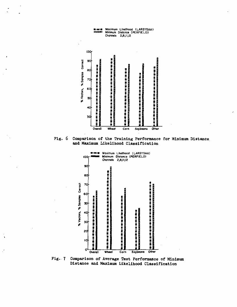
classes: Wheat, Corn, Soybeans andOther were U, 10, 6 and 10 respective-ly. Density histogram estimates ofthe resulting k wheat subclasses areshown in Fig. 5. Note that even afterclustering considerable evidence ofmultimodality still exists, particu-larly for the first subclasses. Infact in some channels the contributionof all h acres assigned to subclass 1are clearly evident. It is possiblethat this data should have been segre-gated into a greater number of sub-classes. After the subclasses hadbeen defined by clustering the statis-tics (means and covariance) were com-puted for each subclass. The featureselection capability of LARSYSAA^^ vasthen used to select the "best" U of the13 channels for classification. Thisselection is based on the average di-vergence between all possible subclasspairs, excluding subclass pairs fromthe same class. On this basis channels2, 8, 11, and 12 were selected. Usingthese channels both the training acresas well as the test fields were class-ified both with LARSYSAA and PERFIELD.The classification results for thetraining acres are shown in Fig. 6while the results for the test fields(again averaged over the 3 flightlines)are shown in Fig. 7-

Discussion of Experimental Results

It is suggested that in evaluatinga classifier a reasonable index of com-parison is the overall average classi-fication accuracy. This performanceindex has the advantage that it givesan indication of the classificationaccuracy that might be expected fromthe classifier for similar data andtraining procedures. For a relativelysmall data set, it is usually rela-tively easy to devise a training pro-cedure or classifier which superfici-ally looks superior but whose apparentsuperiority disappears when resultsare averaged over a number of datasets. A disadvantage of the suggestedperformance index is the necessity todo a reasonable number of classifica-tions .

On the basis of average classifi-cation accuracy and the training pro-cedures used there is no evidence thatthe parametric minimum distance class-ifier is superior to the nonparametricclassifier. Neither is there any evi-dence that using a relatively largenumber of subclasses improves classifi-cation accuracy on the average. Thisis contrary to expectations.

Actually when each field istreated as a subclass one would expectthe nonparametric classifier to per-form better than the parametric class-ifier only if the Gaussian assumptionwas seriously violated for the varioustraining or test fields involved.Futhermore, for the nonparametricclassifier to exhibit any real advan-tage the nonnormal structure of thedata must bear some resemblence fromfield to field (e.g. modes must appearin same relative positions). Since thenonparametric classifier does not ex-hibit any superior performance neitherof the above factors apparently occurwith any consistency.

When the data from all the train-ing fields is grouped one would expectthat the data would be multimodal andthat the nonparametric classifier wouldbe much superior. The basic fallacyin this reasoning appears to be thatalthough the class distributions aremultimodal the samples to be classifiedare usually unimodal. In other wordsthe distribution of any sample to beclassified is not really a random sam-ple from the distribution of any class .Instead it simply tends to account forone of the modes in the class distri-bution. Futhermore, there is no appar-ent way of rectifying this situationwithin the constraint of minimum dis-tance classification.

The fact that the parametricclassifier does so well (comparatively)when no subclasses are consideredattests to the robustness* of the

* A robust classifier is relativelyinsensitive to the underlying assump-tions about the distributions involved.

17

Gaussian assumption in minimum distanceclassification.

It must be recognized that inassessing a classifier factors otherthan the performance index consideredare of importance. One other factorthat should be considered is the con-sistency of the results. That is, hownear to the average can one expect toget for any given classification. Thevariance in the average performance isa measure of this consistency. In thisregard, although the number of classi-fications is small, there is evidencethat the nonparametric classifier isbetter than the parametric version andthat for the parametric classifier thevariance in average performance is in-creased by combining the data frommany fields. This small advantagehardly warrants the additional complex-ity of the nonparametric implementa-tion.

The results comparing the minimumdistance and maximum likelihood class-ifiers show fairly conclusively thatin general the sample classificationaccuracy of minimum distance classi-fiers is higher than the vector class-ification accuracy of maximum likeli-hood classifier of the same data.This is true for both the test andtraining data. It is recognized ofcourse that the quantities being com-pared are by nature somewhat differentbut nevertheless they represent thenatural method of expressing the class-ification accuracy of each classifierindividually and do afford some measureof comparison. This result agrees withexpectations although a greater improve-ment might have been anticipated.

It is convenient to define thedifference between the sample classi-fication accuracy and the vectorclassification accuracy as the improve-ment factor. The exact value of theimprovement factor depends on the par-ticular data but qualitatively it isobvious that for Type II case (a) pro-blems the improvement will be verysmall or non existent both when theseparation of the parameter space

densities for all classes is large(one can't improve a high vector class-ification accuracy much) as well aswhen no separation exists (subclassesof different main classes can then notbe distinguished by either classifier).The experimental evidence suggest thatfor moderate overlap of the parameterspace densities the improvement factorwill be of the order of 5% to 10%.

In concluding it should be men-tioned that no comparative computationtimes have been given. The fact thatthe experiments involved a number ofdifferent programs, two computer sys-tems (one in a time sharing mode) andthe inherent dependence of processingtime on the Classification Parametersand on the manner in which the datais stored (data retrieval time is byno means negligible) makes it virtual-ly impossible to give meaningful com-parative times. Suffice it to saythat to classify a typical flightlinetime would be measured in fractions ofan hour to hours on an IBM 360 SystemModel UU, and that PERFIELD is thefastest classifier, followed byLARSYSDC and LARSYSAA in that order.

CLOSURE

Although only two examples havebeen presented numerous other classi-fications have been performed on simi-lar data and the results generallysupport the results presented. Evenconsidering only the classificationdiscussed the volume of data involvedis quite substantial and is certainlyadequate for a reasonable test.

For the type of data consideredtwo basic conclusions appear reason-able.

(l) The classification accuracy of anonparametric minimum distance classi-fiers, utilizing density histogramsfor estimating pdf's, is on the averagenot any larger than the classificationaccuracy of the parametric (Gaussian)classifier based on parametricallyestimated pdf's. The variability in

18

performance of the nonparametric class-ifier appears somewhat smaller. Sincethe parametric classifier requires lessstorage and is faster than the nonpara-metric classifier the latter classifieris not an attractive alternative.

(2) The average sample classificationaccuracy of a parametric (Gaussian)minimum distance classifier is largerthan the average vector classificationaccuracy of a miximum likelihood vectorclassifier. Ignoring the problem ofsample definition the minimum distanceclassifier is faster and is an attrac-tive alternative to the maximum like-lihood classifier in situations whereit can be utilized.

The disparity between test andtraining results for both minimum dis-tance and maximum likelihood classi-fiers is much greater than the differ-ence due to classifier type or thespecific implementation. This suggeststhat given the present state of the artgreater improvement in classificationaccuracies will probably result frominvestigations intended to improve thetraining procedure than from investi-gation of classifier types.

REFERENCES

D.A. Landgrebe, "Systems Approachto the Use of Remote Sensing",LARS Information Note 01*1571 ,-Purdue University, Lafayette,Indiana, April, 1971.

oA.G. Wacker and D.A. Landgrebe,

"Boundaries in MultispectralImagery by Clustering," 1970IEEE Symposium on AdaptiveProcesses (9th) Decision andControl, pp. XlU.l-XlU.8,December, 1970.

3. R.L. Kuehn, E.R. Omberg and G.D.Forry, "Processing of ImagesTransmitted from ObservationSatellites, "Information Dis-play, Vol. 8, No. 5, pp. 13--17, September/October, 1971,

4. A.G. Wacker, "Minimum DistanceApproach to Classification,"Ph.D. Thesis, Purdue Univer-sity, Lafayette, Indiana,January, 1972. Also availableas LARS Information Note100771, Purdue University,Lafayette, Indiana, October,1971.

5. Z.W. Birbaum, "Distribution FreeTests of Fit for ContinuousDistribution Functions," Ann.Math. Stat., Vol. 2U, pp. 1-8,1953.

6. E. Samuel and R. Bachi, "Measuresof Distances of DistributionFunctions and Some Applica-tions," Metron, Vol. 23, pp.83-122, December, 196U.

7. H. Cramer, "On the Composition ofElementary Errors," Skand.Aktuarietids, Vol. 11, pp. 13-7U and lUl-180, 1928.

8. R. Von Mises, "Wahrscheinlich-keitsrechnung," Leipzig-Wein,1931.

9. D.A. Darling, "The Kolmogorov-Smirnov, Cramer-Von MisesTests," Ann. Math. Stat., Vol.28, pp. 823-838, December,1957- • . '

10. W. Sahler, "A Survey on Distribu-tion-Free Statistics Based onDistances Between DistributionFunctions," Metrika, Vol. 13,pp. 1 9-169, 1968.

1!. A.N. Kolmogorov, "Sulla Determina-zione Empirica Di Une Legge DiDistribuzione," Giorn, dell'Insi

Distribuzione," Giorn,dell'Insit. degli att., Vol.It, pp. 83-91, 1933.

12. N.V. Smirnov, "On the Estimationof the Discrepancy BetweenEmpirical Curves of Distribu-tion for Two Independent

19

13

15

16

18

19

20

21

Samples," Bull. Math. Univ.Moscow, Vol. 2, pp. 3-11*, 1939.

H. Jeffreys, "An Invariant forthe Prior Probability in Esti-mation Problems," Proc . Roy.Soc. A., Vol. 186, pp. U5U-U61,

H. Jeffreys, "Theory of Probabili-ty," Oxford University Press,

T. Kailath , "The Divergence andBhattacharyya Distance Mea-sures in Signal Selection,"IEEE Trans, on Comm. Tech.,Vol. COM-15, pp. 52-60,February, 196?.

A. Bhattacharyya, "On a Measure ofDivergence Between Two Statis-tical Populations Defined byTheir Probability Distribu-tions," Bull. Calcutta Math.Soc., Vol. 35, PP. 99-109, 19 3.

17. K. Matusita, "On the Theory ofStatistical Decision Functions,"Ann Instit. Stat. Math.(Tokyo), Vol. 3, pp. 17-35,1951.

B.P. Adhikari and D.D. Joshi,"Distance Discrimination etResume Exhaustif," Fbls. Inst.Stat., Vol. 5, pp. 57-7 ,1956.

C.H. Kraft, "Some Conditions forConsistency and Uniform Con-sistency of Statistical Pro-cedures," University ofCalifornia Publications inStatistics, 1955.

S. Kullback and R.A. Leiber, "OnInformation and Sufficiency,"Ann. Math. Stat., Vol. 22,pp. 79-86, 1951.

P.H. Swain and K.S. Fu, "Nonpara-metric and Linguistic Ap-proaches to PatternRecognition," LARS InformationNote 051970, Purdue University,Lafayette, Indiana, June, 1970.

21. P.H. Swain and K.S. Fu, "Nonpara-metric and Linguistic Ap-proaches to PatternRecognition," LARS InformationNote 051970, Purdue University,Lafayette, Indiana, June, 1970.

22 . P.C. Mahalanobis, "Analysis of RaceMixture in Bengal," J. Asiat.Soc. (India), Vol. 23, pp. 301-310, 1925.

23. P.C. Mahalanobis, "On the General-ized Distance in Statistics,"Proc. Nat'l. Inst. Sci. (India),Vol. 12, pp. 1+9-55, 1936.

24 . J. Keifer and J. Wolfowitz, "Con-sistency of the Maximum Like-lihood Estimator in thePresence of Infinitely ManyIncidental Parameters," Ann.Math. Stat., Vol. 27, pp. 887-906, 1956.

25. S.M. All and S.D. Silvey, "AGeneral Class of Coefficientsof Divergence of one Distri-bution From Another," J. Roy.Stat. Soc., Ser. B, Vol. 28,pp. 131-1U2, 1966.

26 . D.G. Lainiotis, "On a General Re-lationship Between Estimation,Detection, and theBhattacharyya Coefficient,"IEEE Trans, on InformationTheory,'Vol. IT-15, pp. 50U-505, July, 1969.

27 . C. Stein, "Approximations of Impro-per Prior Probability Measures,"Dept. of Statistics, StanfordUniversity, Stanford, California,Tech. Report 12, 196U.

28. K. Matusita, "On Theory of Statis-tical Decision Functions,"Ann. Inst. Math. (Tokyo), Vol.3, pp. 17-35, 1951.

29. K. Matusita, "On Estimation by theMinimum Distance Method," Ann.Inst. Stat. Math. (Tokyo), Vol.5, pp. 59-65,

20

30 K.

31

32

33.

37

Matusita, Y. Suzuki , and H.Hudimoto, "On Testing Statis-tical Hypothesis," Ann. Inst.Stat. Math. (Tokyo), Vol. 6,pp. 133-lUl,

K. Matusita and H. Akaike, "Deci-sion Rules Based on the Dis-tance for the Problems ofIndependence Invariance andTwo Samples," Ann. Inst. Stat.Math., Vol. 7, PP- 67-80,1956.

K. Matusita and M. Motoo, "On theFundamental Theorem for theDecision Rule Based on Dis-tance || ||," Ann. Inst. Stat.Math., Vol. 7, PP. 137-1 2,1956.

K. Matusita, "Decision Rule Basedon the Distance for the Class-ification Problem," Ann. Inst.Stat. Math. (Tokyo), Vol. 8,pp. 67-70, 1956.

K. Matusita, "Distance and DecisionRules," Ann. Inst. Stat. Math.(Tokyo), Vol. 5, PP. 59-65,195U.

35. K. Matusita, "Classification Basedon Distance in MultivariateGaussian Case," Proc. 5thBerkeley Symposium on Math.Stat. and Prob., Vol. 1, pp.299-301+, 1967.

36. J. Wolfowitz, "Consistent Estima-tions of the Parameters in aLinear Structural Relationship,"Skand. Aktuarietids, pp. 132-151, 1952.

39

40

i+l

44

45

J. Wolfowitz, "The Minimum DistanceMethod," Ann. Math. Stat. Vol.28, pp. 75-88, 1957-

S. Das-Gupta, "Nonparametric Class-ification Rules," Sankhya,Indiana Jour, of Stat., Series

Indian Jour, of Stat., SeriesA, Vol. 26, pp.lf-30,. .1961*.

T. Cacoullos, "Comparing MahalanobisDistance I: Comparing Dis-tances between Populations andAnother Unknown," Sankhya,Indian Jour. Stat., Series A,Vol. 27, pp. 1-22, March, 1965.

T. Cacoullos, "Comparing MahalanobisDistancesII: Bayes ProceduresWhen the Mean Vector are Un-known," Sankhya, Indian Jour.Stat., Series A, Vol. 27, pp.23-32, March, 1965.

M.S. Srivastava, "Comparing Dis-tances Between MultivariatePopulations - The Problem ofMinimum Distance," Ann. Math.Stat., Vol. 38, pp. 550-556,April, 1967.

W. Hoeffding and J. Wolfowitz,"Distinguisability of Sets ofDistributions," Ann. Math.Stat., Vol. 29, pp. 700-718,September, 1958.

K.S. Pu, D.A. Landgrebe, and T.L.Phillips, "Information Pro-cessing of Remotely SensedAgricultural Data," Proc. IEEE,Vol. 57, PP. 639-65 , April,1969.

J. Wolfowitz, "Estimation by theMinimum Distance Method," Ann.Inst. Stat. Math. (Tokyo),Vol. 5, pp. 9-23, 1953.

38. J. Wolfowitz, "Estimation by theMinimum Distance Method inWonparametric DifferenceEquations," Ann. Math. Stat.,Vol. 25, pp. 203-217,

Sensor Coprocessing Form Image Analysis H Results

Image Oriented

Numerically Oriented

Fig. 1 Organization of Image and Numerically Oriented Systems

Pixel

S* \

SpectralBandI

\ \\ \

.Observation Vector (x,,x2,x3,...)

Fig. 2 Formation of Multispectral Data-Image

TIPPECANOE COUNTY. INDIANS

TIPPKCANOB COUNTY HIGHWAY MAP

ih i i ! i i i I i i if I i I i I I i I I f ill

Fig. 3 Location of Tippecanoe County Flightlines 21, 23 and 2k

100

90

80

70

8 60

I««a>a.

3*

50

40

30-

20-

10

0

Parametric Nonparametric• "• With Subclasses *w With Subclassesmimi No Subclasses ^^ No Subclasses

Channels 1,8,11

Us Ss KE 8

is15S

iiimi

iiim

iiiiiiiiiiiiiiiiiiiiiiiiiiiiiiiiiiiiiiiiiiiiiiiiiiiiii

IS

11HHMi?I?

-jl

i!a 5

Iii i= s= 9= sMijIli

Overall Wheat Corn Soybeans Other

Fig. U Comparison of Average Test Performancefor Parametric and Nonparametric MinimumDistance Classification Using BhattacharyyaDistance and Random Training

I

2

3

4

5

6oc

I 7o8

10

I I

12

13

1==

'= .,

Class

Fig. 5 Histograms for Wheat Subclasses Obtained as Result of Clustering Wheat Acres

Maximum Likelihood (LARSYSAA)Minimum Distance (PERFIELD)Channels 2,8,11,12

100

g 90

80M

11 70

CO

38jf 60

I 50

40

30

Overall Wheat Corn Soybeans Other

Fig. 6 Comparison of the Training Performance for Minimum Distanceand Maximum Likelihood Classification

• IBIB Maximum Likelihood (LARSYSAA)I00r •«• Minimum Distance (PERFIELD)

Channels 2,8,11,12

9U

80

g 70

1 6Q

»«

| 4°

20

10

n

•

•

I

'

i

•

i

Overall Wheat Corn Soybeans Other

Fig. 7 Comparison of Average Test Performance of MinimumDistance and Maximum Likelihood Classification