The Langlands Program Seminar

Tian An Wong

July 29, 2016

Abstract

These are notes from the ongoing Langlands Program Seminar organized since Spring 2014. What isknown today as the Langlands Program, originating in a letter from Langlands to Weil in 1967, is nowa vast area of research. While it asks questions of largely number theoretic interest, its methods haverequired input from harmonic analysis, representation theory, algebraic geometry, algebraic numbertheory, and more. Regarding emphasis, I have used as a guide the expository writing of Langlands, andas a result we have focused on functoriality via the trace formula, and reciprocity in terms of motives.These notes are produced by a naive graduate student and there are mistakes scattered throughout, souse them at your own risk! Please direct feedback and comments to twong at gradcenter.cuny.edu.

Contents

1 Basic objects 41.1 Automorphic Representations . . . . . . . . . . . . . . . . . . . . . . . . . . . . . . . . . 41.2 The L-group . . . . . . . . . . . . . . . . . . . . . . . . . . . . . . . . . . . . . . . . . . . 51.3 The Satake Isomorphism . . . . . . . . . . . . . . . . . . . . . . . . . . . . . . . . . . . . 61.4 The Weil-Deligne group . . . . . . . . . . . . . . . . . . . . . . . . . . . . . . . . . . . . 71.5 Touchstone I: Local Langlands . . . . . . . . . . . . . . . . . . . . . . . . . . . . . . . . 81.6 The automorphic L-function . . . . . . . . . . . . . . . . . . . . . . . . . . . . . . . . . . 111.7 Reductive groups . . . . . . . . . . . . . . . . . . . . . . . . . . . . . . . . . . . . . . . . 111.8 Touchstone II: Functoriality principle . . . . . . . . . . . . . . . . . . . . . . . . . . . . . 13

2 The Arthur-Selberg trace formula 142.1 A first look . . . . . . . . . . . . . . . . . . . . . . . . . . . . . . . . . . . . . . . . . . . 142.2 Coarse expansion . . . . . . . . . . . . . . . . . . . . . . . . . . . . . . . . . . . . . . . . 152.3 Jacquet Langlands correspondence . . . . . . . . . . . . . . . . . . . . . . . . . . . . . . 172.4 Refinement . . . . . . . . . . . . . . . . . . . . . . . . . . . . . . . . . . . . . . . . . . . 202.5 Invariance . . . . . . . . . . . . . . . . . . . . . . . . . . . . . . . . . . . . . . . . . . . . 212.6 The unramified case . . . . . . . . . . . . . . . . . . . . . . . . . . . . . . . . . . . . . . 22

3 Base change 233.1 GL(2) base change . . . . . . . . . . . . . . . . . . . . . . . . . . . . . . . . . . . . . . . 233.2 Aside I: Weil restriction of scalars . . . . . . . . . . . . . . . . . . . . . . . . . . . . . . . 263.3 Aside II: Chevalley and Satake Isomorphism. . . . . . . . . . . . . . . . . . . . . . . . . 263.4 Aside III: Conjugacy classes in reductive groups . . . . . . . . . . . . . . . . . . . . . . . 273.5 Noninvariant base change for GL(n) . . . . . . . . . . . . . . . . . . . . . . . . . . . . . 273.6 Aside IV: L-group exercise . . . . . . . . . . . . . . . . . . . . . . . . . . . . . . . . . . . 30

1

4 Endoscopy theory 314.1 Warmup on group cohomology . . . . . . . . . . . . . . . . . . . . . . . . . . . . . . . . 314.2 Endoscopic character . . . . . . . . . . . . . . . . . . . . . . . . . . . . . . . . . . . . . . 324.3 Rational representative . . . . . . . . . . . . . . . . . . . . . . . . . . . . . . . . . . . . . 324.4 Endoscopic group . . . . . . . . . . . . . . . . . . . . . . . . . . . . . . . . . . . . . . . . 334.5 Stable distributions . . . . . . . . . . . . . . . . . . . . . . . . . . . . . . . . . . . . . . . 34

5 Fundamental lemma 355.1 Transfer to characteristic p . . . . . . . . . . . . . . . . . . . . . . . . . . . . . . . . . . 355.2 A first example: SO5 and Sp4 . . . . . . . . . . . . . . . . . . . . . . . . . . . . . . . . . 365.3 Examples of GLn Hitchin fibres . . . . . . . . . . . . . . . . . . . . . . . . . . . . . . . . 365.4 An extended example: GLn . . . . . . . . . . . . . . . . . . . . . . . . . . . . . . . . . . 365.5 Another example: SL2 . . . . . . . . . . . . . . . . . . . . . . . . . . . . . . . . . . . . . 405.6 From GLn to reductive groups . . . . . . . . . . . . . . . . . . . . . . . . . . . . . . . . 415.7 Aside I: some geometric representation theory . . . . . . . . . . . . . . . . . . . . . . . . 435.8 Cohomology of the Hitchin base . . . . . . . . . . . . . . . . . . . . . . . . . . . . . . . . 445.9 Aside II: Cohomological definitions . . . . . . . . . . . . . . . . . . . . . . . . . . . . . . 47

6 Beyond Endoscopy 516.1 Introduction (Altug) . . . . . . . . . . . . . . . . . . . . . . . . . . . . . . . . . . . . . . 516.2 Endoscopy and Beyond . . . . . . . . . . . . . . . . . . . . . . . . . . . . . . . . . . . . 536.3 The test case: GL2 . . . . . . . . . . . . . . . . . . . . . . . . . . . . . . . . . . . . . . . 556.4 The elliptic terms . . . . . . . . . . . . . . . . . . . . . . . . . . . . . . . . . . . . . . . . 566.5 Geometrization: Frenkel-Langlands-Ngo . . . . . . . . . . . . . . . . . . . . . . . . . . . 616.6 Aside: Poisson summation . . . . . . . . . . . . . . . . . . . . . . . . . . . . . . . . . . . 656.7 The story so far (Altug) . . . . . . . . . . . . . . . . . . . . . . . . . . . . . . . . . . . . 666.8 The r-trace formula . . . . . . . . . . . . . . . . . . . . . . . . . . . . . . . . . . . . . . 676.9 Singularities and transfer . . . . . . . . . . . . . . . . . . . . . . . . . . . . . . . . . . . 69

7 Galois Representations 727.1 What are they . . . . . . . . . . . . . . . . . . . . . . . . . . . . . . . . . . . . . . . . . 727.2 L-functions for Galois representations . . . . . . . . . . . . . . . . . . . . . . . . . . . . 737.3 Automorphy . . . . . . . . . . . . . . . . . . . . . . . . . . . . . . . . . . . . . . . . . . . 757.4 An infinite fern . . . . . . . . . . . . . . . . . . . . . . . . . . . . . . . . . . . . . . . . . 777.5 The eigencurve . . . . . . . . . . . . . . . . . . . . . . . . . . . . . . . . . . . . . . . . . 797.6 p-adic Galois representations and p-adic differential equations (Kramer-Miller) . . . . . 80

8 Motives 848.1 Grothendieck motives . . . . . . . . . . . . . . . . . . . . . . . . . . . . . . . . . . . . . 848.2 The Standard Conjectures (Ray Hoobler) . . . . . . . . . . . . . . . . . . . . . . . . . . 858.3 Aside I: Fundamental groups and Galois groups . . . . . . . . . . . . . . . . . . . . . . . 888.4 Aside II: Tannakian categories . . . . . . . . . . . . . . . . . . . . . . . . . . . . . . . . 908.5 The motivic Galois group: examples . . . . . . . . . . . . . . . . . . . . . . . . . . . . . 958.6 The Taniyama group . . . . . . . . . . . . . . . . . . . . . . . . . . . . . . . . . . . . . . 968.7 The automorphic Langlands group . . . . . . . . . . . . . . . . . . . . . . . . . . . . . . 998.8 Motivic homotopy theory . . . . . . . . . . . . . . . . . . . . . . . . . . . . . . . . . . . 103

9 Reciprocity 1059.1 A historical overview . . . . . . . . . . . . . . . . . . . . . . . . . . . . . . . . . . . . . . 1059.2 Explicit reciprocity laws and the BSD conjecture (Florez) . . . . . . . . . . . . . . . . . 1079.3 Non-abelian reciprocity laws on Riemann surfaces (Horozov) . . . . . . . . . . . . . . . 1089.4 An n-dimensional Langlands correspondence . . . . . . . . . . . . . . . . . . . . . . . . . 1109.5 A survey of the relationship between algebraic K-theory and L-functions (Glasman) . . 112

2

9.6 The Stark conjectures . . . . . . . . . . . . . . . . . . . . . . . . . . . . . . . . . . . . . 1159.7 Semistable abelian surfaces of given conductor (Kramer) . . . . . . . . . . . . . . . . . . 118

10 Stable homotopy theory 12010.1 Manifolds and modular forms . . . . . . . . . . . . . . . . . . . . . . . . . . . . . . . . . 12010.2 Stable homotopy groups of spheres . . . . . . . . . . . . . . . . . . . . . . . . . . . . . . 12210.3 The Adams conjecture . . . . . . . . . . . . . . . . . . . . . . . . . . . . . . . . . . . . . 12510.4 Chromatic homotopy theory . . . . . . . . . . . . . . . . . . . . . . . . . . . . . . . . . . 12710.5 Topological modular forms . . . . . . . . . . . . . . . . . . . . . . . . . . . . . . . . . . . 129

11 Appendix 13011.1 Structure theory of algebraic groups . . . . . . . . . . . . . . . . . . . . . . . . . . . . . 130

12 Some references 130

3

1 Basic objects

1.1 Automorphic Representations

1.1. We begin with the classical theory of theta series:

θ(z) =

∞∑n=−∞

eπin2z

with functional equation θ(−1/z) = (−iz)1/2θ(z), proven by the Poisson summation. Riemann usedthis to prove the functional equation for Riemann’s zeta function:

ζ(s) =

∞∑n=1

1

ns=∏p

1

1− p−s.

Riemann showed that the completed zeta function ξ(s) is a Mellin transform:

ξ(s) = π−s2 Γ(

s

2)ζ(s) =

∫ ∞0

θ(it)− 1

2ts−1dt

and using the functional equation of θ(z), the functional equation for ζ(s) follows: ξ(s) = ξ(1− s).

1.2. Next we define a modular form of weight k for G = SL(2,R) with discrete subgroup Γ = SL(2,Z)or some congruence subgroup to be a holomorphic f(z) on the upper-half plane H with transformationlaw

f(γ(z)) = f(az + d

cz + d

)= (cz + d)kf(z), γ =

(a bc d

)∈ Γ.

Thus we can think of modular forms as representations of SL(2,Z)\SL(2,R) by lifting f(z) to φf (g),requiring φf to be left-invariant under SL(2,Z), right-SO(2,R) finite, an eigenfunction of the Casimiroperator, and satisfying a certain slow-growth condition.

More generally, an automorphic form of weight k for a topological group G with discrete subgroupΓ to be a function f(γ(z)) = j(γ, z)kf(z) where j(γ, z) is called a factor of automorphy, satisfying asimilar growth, eigenfunction and invariance conditions. Denote A the space of automorphic forms.

1.3. Hecke generalized Riemann’s proof as follows: let an be a sequence of complex numbers withan = O(nc) for c > 0, and let h > 0, k > 0, λ > 0, C = ±1, and define

f(z) =

∞∑n=0

ane2πinz/h, φ(s) =

∞∑n=1

anns, f(z), and Φ(s) = (

λ

2π)sΓ(s)φ(s)

Theorem 1.1.1. The following are equivalent:(i) Φ + a0/s+ C/(k − s) is entire, bounded on vertical strips, and satisfies Φ(k − s) = CΦ(s)(ii) f(−1/z) = C(z/i)kf(z), i.e., f(z) is an automorphic form of weight k.

The next question asks when a Dirichlet series∑ann

−s has an Euler product∏p Lp(s). Hecke

showed that for Hecke operator Tp acting on the space A, we have the following

Theorem 1.1.2. Assume, for convenience, that f(z) =∑ane

2πinz is a modular form for SL(2,Z)and a1 = 1. Then f is an eigenfunction of Tp for all p, i.e.,

Tpf(z) = pk−1∑

Γ\Mm

j(γ, z)kf(γ(z)) = apf(z)

if and only if the an are multiplicative, i.e., if amn = aman whenever m,n are relatively prime.

4

As a corollary of the multiplicativity of the an, φ(s) will have an Euler product as follows:

φ(s) =∏p

Lp(s) =∏p

(1− app−s + pk−1−2s)−1

1.4. Tate, in a different setting, proved the functional equation for a Hecke L-function using adelicmethods. Recall the adele ring of a number field F to be AF =

∏′v Fv, where Fv is a local field

completed at the prime v, and product is the restricted direct product, where almost all factors are Ov,the ring of integers of Fv. In particular, is F = Q we have AQ = R×

∏′Qp, where p are finite primes.This analysis follows in the spirit of Hasse’s local-global principle.

Now fix a Hecke character χ : F×\A×F → C× (a one dimensional representation of GL(1,A)) suchthat χ(x) =

∏χv(xv) where χv is trivial on units (unramified) for almost all v. Also define a Schwartz-

Bruhat function f(x) =∏fv(xv) where fv is Schwartz if v is an infinite prime, and locally constant

compactly supported when v is finite. In summary, Tate defined a local zeta function

ζ(fv, χv, s) =

∫F×v

fv(x)χv(x)|x|s−1dx

and using Poisson summation and an appropriately defined Fourier transform for functions on numberfields, proved a functional equation and analytic continuation ζ(fv, χv, s) = γ(χv, s)ζ(fv, χ

−1v , 1 − s)

where γ(χv, s) (local gamma factor) is a meromorphic function of s. Then considering the global zetafunction ζ(f, χ, s) =

∏ζ(fv, χv, s) Tate showed that Hecke’s L-series

L(s, χ) =∏v

L(s, χv) =∏

v unram

(1− χv(ω)N(p)−s)−1

has an analytic continuation and functional equation L(χ, s) = ε(s, χ)L(1 − s, χ−1) with ε(s, χ) =∏ε(s, χv) and ε(s, χv) = 1 when χv is unramified.

1.5. Now we define an automorphic representation by making A into a Hecke algebra H moduleas follows. For each finite place v let Hv be the convolution algebra of complex valued locally constantfunctions compactly supported onG(Fv), with Haar measure normalized to give G(Ov) measure 1, sothat the characteristic function of G(Ov) is an idempotent Iv in Hv. Now form the restricted tensorproduct Hf of Hv with respect to Iv for all finite places v, by taking product functions that are Ivat almost every place. Next let H∞ be the convolution algebra of all K∞ finite distributions on G∞supported on K∞, a maximal compact subgroup. Then define H = H∞ ⊗Hf , so that A is a smoothright H-module, and an automorphic representation of H is any irreducible subquotient of A. IfA0 is the space of cusp forms, then any irreducible subquotient of A0 as an H-module is a cuspidalautomorphic representation.

1.2 The L-group

2.1. Let k be a field, with algebraic closure k. There is a canonical bijection between isomorphismclasses of connected reductive k-groups and isomorphism classes of root systems: associate to G theroot datum (X∗(T ),Φ, X∗(T ),Φ∨) where T is a maximal torus in G, X∗(T ) the group of characters ofT , Φ the set of roots of G with respect to T . The choice of a Borel subgroup is equivalent to that of abasis ∆ of Φ, whence a bijection between isomorphism classes of (G,B, T ) and isomorphism classes ofbased root data ψ(G) = (X∗(T ),∆, X∗(T ),∆∨).

To the k-group G we first associate the group G over C such that ψ(G) = ψ(G)∨, the dual rootdatum of G. Similarly we obtain B and T . Let f : G → G′ be a k-morphism, whose image is anormal subgroup. Then f induces maps ψ(f) : ψ(G)→ ψ(G′) and ψ∨(f) : ψ(G′)∨ → ψ(G)∨, and thusf∨ : G′∨ → G.

For example, if G = GLn, SLn, Sp2n then G = GLn(C), PGLn(C), S)2n+1(C).

5

2.2. Given γ ∈ Gal(ks/k) = Γk there is a g ∈ G(ks) such that gγTg−1 = T thus an automor-phism of ψ(G) depending only on γ. So we have a homomorphism µG : Γk → Aut ψ(G). If G′ is ak-group isomorphic to G over k, then µG = µG′ if and only if G,G′ are inner forms of each other. Wehave canonically Aut ψ(G) = Aut ψ(G)∨, hence we may view µG descends to a map µ′G to Aut ψ(G)∨.There is a split exact sequence

1 −→ Int G −→ Aut G −→ ψ(G) −→ 1

where any two splittings differ by an inner automorphism. So choose a monomorphism of Aut ψ(G)∨

to Aut (G, B, T ). Then define the L-group of G to be L(G/k) = LG = GoΓk with respect to µ′G, welldefined up to inner automorphism. We have the split exact sequence

1 −→ G −→L G −→ Γk −→ 1

If G splits over k, then Γk acts trivially on G and LG = G × Γk. There will be many variants of thisnotion, replacing Γk by a group more suited to the context at hand. A representation of LG will bea continuous homomorphism r : LG → GLn(C) whose restriction to G is a morphism of complex Liegroups.

1.3 The Satake Isomorphism

3.1. Let G be a connected reductive group over a local field k. Fix a maximal k-split torus S withcentralizer M , B the Borel subgroup containing S. Let W = NG(S)/ZG(S) be the restricted Weylgroup of S, U and K the unipotent radical and (hyperspecial) maximal compact subgroup of P .

Theorem 1.3.1. (Satake) Define the Satake transform as a linear map S : H(G,K)→ H(M,M ∩K)W by

Sf(m) = δ(m)1/2

∫N

f(mn)dn

for f in H(G,K) and m in M , and δ = |det | is the modulus character. Then S is an isomorphism.

We do not present a proof of the theorem, and note that most expositions of the isomorphism (ex-cept Cartier’s) give only a sketch of the proof.

Proposition 1.3.2. If G is split, then H(M,M ∩K) ' C[X∗(M)].

Proof. Define γ(m) to be the cocharacter such that (γ(m), χ) = ord(χ(m)) for all χ in X∗(M).This gives an exact sequence

1 −→M(O) −→M(k) −→ X∗(M) −→ 0

To get a splitting of the sequence, we first note that each function in H(G,K) is constant on double Kcosets, it is also compactly supported and hence a finite linear combination of characteristic functions1KgK , so that the 1KgK are a basis for H(G,K). Given λ in X∗(M) and $ uniformizing element of O,then λ($) belongs to T (k), and since λ(O×) ⊂ T (O) ⊂ K the double coset Kλ($)K does not dependon choice of $. Then the mapping λ to 1Kλ($)K gives the splitting M(k)/M(O) ' X∗(M). Then byconsidering the group algebra C[X∗(M)] = C[M(k)/M(O] = C[M/M ∩K] as the convolution algebraof functions from M/M ∩K to C, hence H(M,M ∩K).

Proposition 1.3.3. There is a canonical identification X∗(M) ' X∗(M∨).

Proof. Let M∨(C) = Hom(M(k)/M(O),C×). Then from the above splitting we have the iden-tification M∨(C) = Hom(X∗(M),C×). Also, given a complex torus M(C) we can identify it withHom(X∗(M),C×) by duality. So Hom(X∗(M∨),C×) ' Hom(X∗(M),C×), hence X∗(M) ' X∗(M∨).

6

Theorem 1.3.4. (Chevalley) If G is a complex connected reductive group with maximal torus M∨ andWeyl group W , then the restriction regular functions on G to M∨ induces an isomorphism C[G]G 'C[M∨]W .

A basis for conjugation invariant rational functions on G is given by characters of irreducible highestweight algebraic representations, spanning a Z-lattice inside C[G]G, which can be identified with thealgebra of isomorphism classes of virtual representations of G. The positive roots in X∗(M∨) indexirreducible representations Vλ of G, viewing Tr(Vλ) as an element of C[X∗(M∨)] = Rep(G).

Proposition 1.3.5. There is a bijection between characters of H(G,K) and unramified characters χof M .

A representation (π, V ) of G is smooth if every vector is fixed by a sufficiently small compact opensubgroup. A smooth representation is spherical or unramified with respect to K if it contains a nonzeroK-fixed vector, i.e., if V K 6= 0. Given an irreducible spherical representation π of G, πK is an irreducibleH(G,K) module. By the Satake isomorphism (or Gelfand’s lemma), H(G,K) is commutative, henceby Schur’s lemma dim πK = 1 and H(G,K) acts by a character.

Conversely, given an unramified character χ of M , we may view it as a character of B and inducethe spherical principal series representation I(χ) = IndGB(δ

12χ), locally constant functions from G to C

such that f(bgk) = δ12 (b)χ(b)f(g). χ is trivial on M ∩K, so by Iwasawa’s decomposition dimχK = 1.

Since (·)K is exact, I(χ) has a unique irreducible spherical sub quotient πχ.

Theorem 1.3.6. (Langlands) M∨/W naturally corresponds to semisimple G conjugacy classes in Goσ.

This was proved by Langlands, which proof we omit here. Finally we have the following identifica-tion:

Corollary 1.3.7. There is a bijection between characters of H(G,K) and semisimple G conjugacyclasses in Go σ.

Concisely, Hom(H(G,K),C) = Hom(H(M,M ∩ K)W ,C) = Hom(C[X∗(M∨)]W ,C) = M∨/W =(Go σ)ss. We will explain the last in the next section.

1.4 The Weil-Deligne group

Let F be a field, F the algebraic separable closure of F . For each finite extension E of F in F , let GE =Gal(F/E). If G is a topological group, Gc is the closure of its commutator subgroup, and Gab = G/Gc

is the maximal abelian Hausdorff quotient of G. We begin with the exact sequence for E,F finite Galoisextensions of Qp:

1 −→ IE/F −→ Gal(E/F ) −→ Gal(kE/kF ) −→ 0

which letting E be F ,

1 −→ IF −→ Gal(F/F ) −→ Gal(kF /kF ) ' Z −→ 0

This is the setting for the local Weil group. We now state the existence theorem of local class fieldtheory:

Theorem 1.4.1. Let E be a finite Galois extension of F . The map E → F×/NE/FE× is a bijection

between finite abelian Galois extensions E of F with finite index open subgroups of F×.

Corollary 1.4.2. The local reciprocity map θF : F× →W abF ⊂ GabF is a topological isomorphism.

The Weil group of F is a topological group WF with a homomorphism ϕ into GF with dense imageand isomorphism rE : CF →W ab

E , where CE = E× if E is local and A×E/E× if E is global, satisfying

(1) For each E, the composition CE∼−→W ab

E

ϕ−→ GabE is the reciprocity law homomorphism.(2) For w in WE and ϕ(w) in WE , conjugation by w or φ(w) commutes with r.

7

(3) For E′ ⊂ E, the inclusion CE′ → CE and transfer homomorphism t : Gab → Hab commute withr.

(4) For E ⊂ F , the natural map WF → lim←−WF /WcE is an isomorphism of topological groups.

where WE = ϕ−1(GE). Continuity of ϕ implies WE is open in WF and dense image means ϕ inducesbijection of homogeneous spaces WF /WE

∼−→ GF /GE ' HomF (E,F ), which is Gal(E/F ) when E/Fis Galois.

Proposition 1.4.3. A unique WF exists for every F .

Now we discuss the Weil group for the following four cases of F :

(1) F local nonarchimedean. For each E let kE be its residue field with degree qE , and k the unionof all kE . We take WF to be the dense subgroup of GF inducing on k the map x→ xq

nE for n integral,

so WF contains the inertia group IF and WF /IF = Z. Toplogize WF such that IF is open with theprofinite topology.

(2) F global function field. This is as above with ‘constan1t field’ for ‘residue field’ and ‘inertiagroup’ for ‘geometric Galois group’.

(3) F local archimidean. If F is complex then WF = C×, ϕ trivial and rF = id. If F is real then wecan take WF = C×∪ jC× with j2 = −1 and jσj−1 = σ, where σ is the nontrivial element of Gal(C/R).ϕ takes C× to 1 and jC× to σ; while rF = id.

(4) F global number field. ϕ is surjective with kernel the connected component of 1 and isomorphicto the inverse limit of connected components of 1 in CE under NE/E′ .

What is the motivation behind this? Local class field theory gives not only an isomorphism between

the completions Gal(F/F )ab and F×

but also between the distinguished dense subgroups WF and F×.Using the isomorphism between CF and W ab

F we can identify characters of CF with those of W abF , and

by the dense image of WF of GF we can identify the isomorphism classes of representations of GF asa subset of those of WF , called ‘of Galois type’.

Furthermore, for a nonarchimidean local field F . We view WF as a group scheme over Q, theinverse limit WF /J over all normal subgroups J of I. Define the Weil-Deligne group (scheme) W ′Fas WF nGa, where WF acts by wxw−1 = ||w||x.

Let E be a field of characteristic 0. A representation of W ′F over E is a homomorphism ρ :WF → GL(V ) with kernel containing an open subgroup of IF (continuous for the discrete topology ofGL(V )), V a finite dimensional vector space over E, and a nilpotent endomorphism N of V such thatρ(w)Nρ(w)−1 = ||w||N . The representation is semi simple if the Frobenius acts semisimply on V .

Let l be a prime different from the residue characteristic of k and G be an algebraic group over QAn l-adic representation of WF is a homomorphism WF → GL(V ) where V is a finite dimensionalvector space over a finite extension El of Ql.

Theorem 1.4.4. (Deligne) There is a natural bijection between l-adic representations of WF andrepresentations of W ′F over El.

Every element x of W ′F has a unique Jordan decomposition x = xsxu = xuxs. Moreover x isunipotent if and only if it is in Ga, semi simple if either x is inertial or ε(x) is nonzero, where ε : W ′F → Z.An admissible homomorphism of W ′F to LG over GF is a continuous homomorphism α such thatα(Ga) is unipotent in G, and if α(W ′F ) is contained in a Levi subgroup of a parabolic subgroup P ,then P is relevant. When G = GLn, α is a semisimple representation of W ′F . Denote Φ(G) the set ofequivalence classes of α up to inner automorphism by elements of G.

1.5 Touchstone I: Local Langlands

5.1. We now arrive at the first milestone: the local Langlands correspondence, or the local Langlandsreciprocity conjecture, or local Langlands for short. First, let’s motivate the conjecture with Artinreciprocity:

8

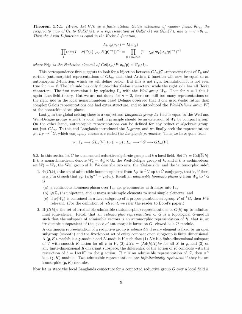
Theorem 1.5.1. (Artin) Let k′/k be a finite abelian Galois extension of number fields, θk′/k thereciprocity map of Ck to Gal(k′/k), σ a representation of Gal(k′/k) on GLC(V ), and χ = σ θk′/k.Then the Artin L-function is equal to the Hecke L-function,

Lk′/k(σ, s) = L(s, χ)∏p

(det(I − σ(FrP )|V IPN(p)−s))−1 =∏

p ramified

(1− χp($p)|ok/p|−s)−1

where Fr|P is the Frobenius element of Gal(ok′/P ; ok/p) ' GP /IP .

This correspondence first suggests to look for a bijection between GLn(C)-representations of Γk andcertain (automorphic) representations of GLn, such that Artin’s L-function will now be equal to anautomorphic L-function, which we will define below. But this is not right formulation; it is not eventrue for n = 1! The left side has only finite-order Galois characters, while the right side has all Heckecharacters. The first correction is by replacing Γk with the Weil group Wk. Then for n = 1 this isagain class field theory. But we are not done: for n = 2, there are still too many representations onthe right side in the local nonarchimidean case! Deligne observed that if one used `-adic rather thancomplex Galois representations one had extra structure, and so introduced the Weil-Deligne group W ′kat the nonarchimedean places.

Lastly, in the global setting there is a conjectural Langlands group Lk that is equal to the Weil andWeil-Deligne groups when k is local, and in principle should be an extension of Wk by compact group.On the other hand, automorphic representations can be defined for any reductive algebraic group,not just GLn. To this end Langlands introduced the L-group, and we finally seek the representationsϕ : LF → LG, which conjugacy classes are called the Langlands parameter. Thus we have gone from

σ : Γk −→ GLn(V ) to (r ϕ) : LF −→ LG −→ GLn(V ).

5.2. In this section let G be a connected reductive algebraic group and k a local field. Set Γk = Gal(k/k).If k is nonarchimedean, denote W ′k = W ′k n Ga the Weil-Deligne group of k, and if k is archimedean,set W ′k = Wk, the Weil group of k. We describe two sets, the ‘Galois side’ and the ‘automorphic side’:

1. Φ(G(k)): the set of admissible homomorphisms from LF to LG up to G-conjugacy, that is, if thereis a g in G such that gϕ1(w)g−1 = ϕ2(w). Recall an admissible homomorphism ϕ from W ′k to LGis

(a) a continuous homomorphism over Γk, i.e, ϕ commutes with maps into Γk,

(b) ϕ(Ga) is unipotent, and ϕ maps semisimple elements to semi simple elements, and

(c) if ϕ(W ′k) is contained in a Levi subgroup of a proper parabolic subgroup P of LG, then P isrelevant. (For the definition of relevant, we refer the reader to Borel’s paper.)

2. Π(G(k)): the set of irreducible admissible (automorphic) representations of G(k) up to infinites-imal equivalence. Recall that an automorphic representation of G is a topological G-modulesuch that the subspace of admissible vectors is an automorphic representation of H, that is, anirreducible subquotient of the space of automorphic forms on G, viewed as a H-module.

A continuous representation of a reductive group is admissible if every element is fixed by an opensubgroup (smooth) and the fixed-point set of every compact open subgroup is finite dimensional.A (g,K)-module is a g-module and K-module V such that (1) Kv is a finite-dimensional subspaceof V with smooth K-action for all v in V , (2) kXv = (Ad(k)X)kv for all X in g, and (3) onany finite-dimensional K-invariant subspace, the differential of the action of K coincides with therestriction of k = Lie(K) to the g action. If π is an admissible representation of G, then πK

is a (g,K)-module. Two admissible representations are infinitesimally equivalent if they induceisomorphic (g,K)-modules.

Now let us state the local Langlands conjecture for a connected reductive group G over a local field k.

9

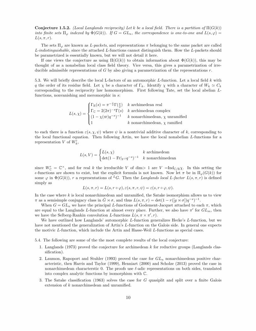
Conjecture 1.5.2. (Local Langlands reciprocity) Let k be a local field. There is a partition of Π(G(k))into finite sets Πϕ indexed by Φ(G(k)). If G = GLn, the correspondence is one-to-one and L(s, ϕ) =L(s, π, r).

The sets Πϕ are known as L-packets, and representations π belonging to the same packet are calledL-indistinguishable, since the attached L-functions cannot distinguish them. How the L-packets shouldbe parametrized is essentially known, but we will not detail it here.

If one views the conjecture as using Π(G(k)) to obtain information about Φ(G(k)), this may bethought of as a nonabelian local class field theory. Vice versa, this gives a parametrization of irre-ducible admissible representations of G by also giving a parametrization of the representations r.

5.3. We will briefly describe the local L-factors of an automorphic L-function. Let a local field k withq the order of its residue field. Let χ be a character of Γk. Identify χ with a character of Wk ' Ckcorresponding to the reciprocity law homomorphism. First following Tate, set the local abelian L-functions, nonvanishing and meromorphic in s:

L(s, χ) =

ΓR(s) = π−

s2 Γ( s2 ) k archimedean real

ΓC = 2(2π)−sΓ(s) k archimedean complex

(1− χ($)q−s)−1 k nonarchimedean, χ unramified

1 k nonarchimedean, χ ramified

to each there is a function ε(s, χ, ψ) where ψ is a nontrivial additive character of k, corresponding tothe local functional equation. Then following Artin, we have the local nonabelian L-functions for arepresentation V of W ′k,

L(s, V ) =

L(s, χ) k archimedean

det(1− Fr|V I q−s)−1 k nonarchimedean

since W ′C = C×, and for real k the irreducible V of dim> 1 are V =IndC/Rχ. In this setting theε-functions are shown to exist, but the explicit formula is not known. Now let π be in Πϕ(G(k)) forsome ϕ in Φ(G(k)), r a representations of LG. Then the Langlands local L-factor L(s, π, r) is definedsimply as

L(s, π, r) = L(s, r ϕ), ε(s, π, r, ψ) = ε(s, r ϕ,ψ).

In the case where k is local nonarchimedean and unramified, the Satake isomorphism allows us to viewπ as a semisimple conjugacy class in Go σ, and thus L(s, π, r) = det(1− r([g o σ])q−s)−1.

When G = GLn we have the principal L-functions of Godement-Jacquet attached to each π, whichare equal to the Langlands L-function at almost every place. Further, we also have π′ for GLm, thenwe have the Selberg-Rankin convolution L-functions L(s, π × π′, r).

We have outlined how Langlands’ automorphic L-function generalizes Hecke’s L-function, but wehave not mentioned the generalization of Artin’s L-function on the Galois side. In general one expectsthe motivic L-function, which include the Artin and Hasse-Weil L-functions as special cases.

5.4. The following are some of the the most complete results of the local conjecture:

1. Langlands (1973) proved the conjecture for archimedean k for reductive groups (Langlands clas-sification).

2. Laumon, Rapoport and Stuhler (1993) proved the case for GLn nonarchimedean positive char-acteristic, then Harris and Taylor (1999), Henniart (2000) and Scholze (2013) proved the case innonarchimedean characterstic 0. The proofs use `-adic representations on both sides, translatedinto complex analytic functions by isomorphism with C.

3. The Satake classification (1963) solves the case for G quasiplit and split over a finite Galoisextension of k nonarchimedean and unramified.

10

1.6 The automorphic L-function

6.1. Let k be a global field with ring of integers O, G a connected reductive k-group. Let π be anirreducible admissible representation of G(A), and r a representation of LG. By a well-known theoremof Flath,

Theorem 1.6.1. Any irreducible admissible representation π of G(A) is uniquely isomorphic ⊗′πvwhere πv is an irreducible admissible representation of G(kv).

Also, by restriction r defines a representation rv of LG(kv). Now assuming the local Langlandscorrespondence, we have a unique ϕv in Φ(G(kv)) such that πv is in Π(G(kv)). Now we define theautomorphic L-function as follows

L(s, π, r) =∏v

L(s, πv, rv), ε(s, π, r) =∏v

ε(s, πv, rv, ψv)

where ψv is a nontrivial additive character of kv, and the local factors are those defined in the previoussection.

Theorem 1.6.2. (Langlands) Let π be an irreducible admissible unitarizable representation of G(A)and r a representation of LG. Then L(s, π, r) converges absolutely for Re(s) large enough.

Now let π be a cuspidal automorphic representation of G(A), hence unitary modulo the center. Itis shown that every cuspidal representation is a constituent of a representation induced from a cuspidalrepresentation of the Levi subgroup of G, yielding

Theorem 1.6.3. (Langlands) Let π be a cuspidal automorphic representation of G(A), and r a repre-sentation of LG. Then L(s, π, r) converges absolutely in some right half-plane.

We say that ϕ in Π(G) is unramified if it is trivial on Ga and the inertia group I, and we mayassume that the image of ϕ lies in LT , and by a property of admissible homomorphsms G is quasisplit.Then Langlands’ interpretation of the Satake isomorphism associates a semisimple conjugacy class ofLG to Hecke algebra character associated to π is represented by to σ.

The following are some examples:

(a) G = GLn, r the standard representation of GLn(C). Then L(s, π, r) satisfies a functionalequation, and for π cuspidal and r irreducible nontrivial, then L(s, π, r) is entire. This is proved inn = 2 by Jacquet and Langlands, and for n ≥ 2 by Godement and Jacquet using ’standard’ L-functionsfor GLn.

(b) G = GLm × GLn where m < n, r = rm ⊗ rn and π × π′ a unitary cuspidal automorphicrepresentation. Then L(s, π × π′, rm ⊗ rn) converges for Re(s) large enough, and extends to an entirefunction of s bounded in vertical strips, satisfying a functional equation.

Converse theorems. To what extent can analytic properties of a given L-function characterize arepresentation? THe first main result was due to Hecke, followed by Weil, and proven in the GL2

setting by Jacquet Langlands, and subsequently for GL3 by Jacquet, Piatetskii-Shapiro and Shalika.

1.7 Reductive groups

LetG be a connected reductive linear algebraic group, fix T a maximal torus ofG. Define a root systemΦ = Φ(G,T ) to be the set of nontrivial characters of T in diagonalizing the adjoint representation of Ton Lie(G).

Associate to (G,T ) the root datum ψ(G,T ) = (X∗(T ),Φ, X∗(T ), Φ). For α in Φ, let Tα be theidentity component of the kernel of α, which is a subtorus of codimension 1. Its centralizer in G isa connected reductive group with maximal torus T , whose derived group Gα is semisimple of rank 1(isomorphic to SL2 or PSL2. There is a unique homomorphism α : Gm → Gα such that T = (Im α)Tαand (α, α) = 2.

11

An isogeny of algebraic groups is a surjective rational homomorphism with finite kernel. Example:The canonical homomorphism of SL2 to PSL2, but in characteristic 2 this is an isomorphism of abstractbut not algebraic groups.

Theorem 1.7.1. (1) For any root datum Ψ with reduced root system there exists a reductive group Gwith maximal torus T in G such that Ψ = ψ(G,T ). The pair (G,T ) is unique up to isomorphism.

(2) Let Ψ = ψ(G,T ) and Ψ′ = ψ(G′, T ′). If f is an isogeny of Ψ′ into Ψ there exists a centralisogeny φ of (G,T ) onto (G′, T ′) with f(φ) = f Two such φ differ by an automorphism Int(t) of G,where t ∈ T .

Now let k be a field. A linear algebraic group defined over k is a k-group, and G(k) its k-rationalpoints. Let G,G′ be k-groups. G′ is a k-form of G if G and G′ are isomorphic over the algebraicclosure. Example: Un is an R-form of GLn.

If G→ GLn is a k-isomorphism of G onto a closed subgroup of GLn, then G(ks) determines G upto k-isomorphism. The k-forms of G, up to isomorphism, are as follows: there is a continuous functionc : s→ cs of Gal(ks/k) to the ks-automorphisms of G such that cst = css(ct). G

′ is an inner form of Gif all cs are inner automorphisms, and G′ is k-isomorphic to G if and only if there is an automorphismc such that cs = c−1sc.

The continuous functions cs above are 1-cocycles of Gal(ks/k) with values in G. Modulo the lastrelation above these form the cohomology H1(k,G).

Let G be a connected reductive k-group. G is quasisplit if it contains a Borel subgroup definedover k, and split (over k) if it contains a maximal k-split torus. Example: SO(Q) is quasiplit but notsplit if and only if the dimension n of the underlying vector space is even and the index is n/2− 1. Gis anisotropic (over k) if it has no nontrivial k-split subtorus. Examples:

(i) Let Q be a nondegenerate quadratic form on a k-vector space (char6= 2), then the identitycomponent SO(Q) of O(Q) is anisotropic if an only if Q is not zero over k.

(ii) If k is locally compact and not discrete, then G is anisotropic over k if and only if G(k) iscompact.

(iii) If k is any field then G is anisotropic if and only if G(k) has no nontrivial unipotent elementsand the group is its k-rational characters Homk(G,Gm) is trivial.

A parabolic subgroup P of an algebraic group G is a closed subgroup such that G/P is a projectivescheme. Equivalently, P is parabolic if P contains a Borel subgroup of G (a maximal Zariski closedand connected solvable algebraic subgroup.).

Let G be a connected reductive k-group an P a parabolic k-subgroup, with unipotent radical N . ALevi subgroup of P is a k-subgroup L such that P = L o N . If A is a maximal k-split torus in thecenter of L then L = Z(A).

The Tits building B: Let G be a connected reductive k-group. The vertices of B are the maximalnontrivial parabolic k-subgroups of G. A set of vertices determine a simplex of if and only if their inter-section is parabolic. A simplex is a face of another simplex if and only if the its parabolic is containedin the other. Maximal simplices (chambers) correspond to minimal parabolics. A codimension-1 faceof a chamber is a wall. G(k) acts on B.

Example: GLn is a reductive k-group. The subgroup A of diagonal matrices is a maximal k-splittorus which is also a maximal torus of G. The ei mapping a ∈ A onto the ith diagonal elementform a basis for X∗(A). The root system consist of ei − ej , i 6= j, and one has the root datum(Zn, ei − ej,Zn, ei − ej). The subgroup B of upper triangular matrices is a minimal parabolic k-subgroup, also Borel. The unipotent radical has ones on the diagonal, upper triangular. The Weylgroup is isomorphic to Sn. The parabolic subgroups P ⊃ B are the upper triangular block matrices,Aii nonsingular, with unipotent radical when Aii = I. The subgroup of P with Aij = 0 for i < j is aLevi subgroup of P .

Let V = kn. A flag in V is a sequence 0 = V0 ⊂ · · · ⊂ Vs = V of distinct subspaces. A k-flag haseach Vi defined over k. GLn acts on the set of all flags; the parabolic subgroups are the isotropy groups

12

of flags, and there is a bijection between parabolic subgroups of G and flags. G/P can be viewed asthe flags of the same type as P , i.e., their subspaces have constant dimension.

If G is an R group, then G(R) is canonically a real Lie group. If G is a C-group then G(C) is acomplex Lie group, and ResC/RG(R) is defined by G(C).

1.8 Touchstone II: Functoriality principle

The principle of functoriality is simple to state, but its implications are many and deep. We begin witha description of functoriality.

Let G and G′ be reductive groups, and ρ : LG → LG′ an L-homomorphism, i.e., commutes withprojection on to the Galois group and is complex analytic over G. Then there should be a correspondenceof automorphic representations π → π′ such that t(πv) and ρ(t(π′v)) are conjugate for almost all v.Moreover, one expects for any finite dimensional representation r′ or LG′ the equality

L(s, π′, r′) = L(s, π, r′ ρ).

We list several key consequences of the conjecture to illustrate its power:

1. G arbitrary, G′ = GLn, reduces the theory for reductive groups to that of GLn. In particular onegets analytic control of their automorphic L-functions through the Godement-Jacquet L-function.

2. G trivial, G′ = GLn, would imply the reciprocity conjecture, yielding the Artin conjecture.

3. G = GL2, G′ = GLn, would imply the Ramanujan conjecture in utmost generality.

4. G = GLn×GLm, G′ = GLnm endows the category of automorphic representations of GLk for allk > 0 the structure of a monoidal category.

Functoriality, conjectured in 1979, has only been established in a very limited number of cases, andthe complete picture is not expected for a long time still. The following are the strongest results towardsfunctoriality:

1. G = GLn(F ), G′ =ResE/FGLn where Gal(E/F ) is cyclic. This result is due to Arthur-Clozel(1989) using the stable trace formula.

2. G = GL2, G′ = GL3, GL4, GL5, symmetric square, cube and fourth by Gelbart-Jqcquet (1978),Kim-Shahidi (2002) and Kim (2003) using converse theorems.

3. G = GL2 × GL2, G′ = GL4, tensor product representation, due to Ramakrishnan (2000) usingthe converse theorem of Cogdell and PS.

4. G = GL2 ×GL3, G′ = GL6, tensor product representation, due to Kim-Shahidi (2002) again byconverse theorem.

In the theory of automorphic forms, one usually carries out a comparison of trace formulas, corre-sponding to two groups. Roughly speaking, a trace formula is an identity

(irreducible characters of G on f) = (orbital integrals of f),

respectively, the spectral and geometric sides. Here f is a properly chosen test function, allowing one tomatch the orbital integrals on both groups, giving cancellation and in the end an identity of characters.In general one has

(cuspidal) + (one-dimensional) + (continuous) + (residual)

= (central) + (elliptic) + (hyperbolic) + (unipotent)

13

2 The Arthur-Selberg trace formula

2.1 A first look

Let Γ be a discrete subgroup of a locally compact unimodular topological group G. Let R be the unitaryrepresentation of G by right translation on L2(Γ\G). Choose a test function f in C∞c (H), and definethe operator

R(f) =

∫G

f(y)R(y)dy

acting on L2(Γ\G) by

R(f)ϕ(x) =

∫G

f(y)ϕ(xy)dy =

∫Γ\G

∑γ∈Γ

f(x−1γy).ϕ(y)dy

so R(f) is an integral operator with kernel

K(x, y) =∑γ∈Γ

f(x−1γy),

where the sum is finite, taken over the intersection of the discrete Γ with the compact subset xsupp(f)y−1.If Γ is cocompact, the kernel is square integrable, so R(f) is a trace class operator and by the

spectral theorem R decomposes discretely into irreducible representations π with finite multiplicity.Taking trace leads to the geometric expansion

trR(f) =

∫Γ\G

K(x, x)dx =

∫Γ\G

∑Γ

∑Γγ\Γ

f(x−1δ−1γδx)dx =∑Γ

vol(Γγ\Gγ)

∫Gγ\G

f(x−1γx)dx,

and the spectral expansion

trR(f) =∑π

m(π)tr(π(f)).

In the notation of Arthur, one has a first identity∑π

aGΓ (π)fG(π) =∑γ

aGΓ (γ)fG(γ).

When G = R, Γ = Z, this is the Poisson summation formula, with irreducible representations e2πinx.In the following we will almost exclusively consider the setting of G = G(A), Γ = G(F ) where G is areductive group and F a number field, or simply Q. In general, ZAGQ\GA is not compact, causing R(f)to not be trace class and R not to decompose discretely. (The quotient is noncopact when G containsa proper parabolic subgroup P defined over Q.)

Selberg introduced the trace formula for G = SL2(R)/SO2, Γ a subgroup of SL2(Z). He studiedthis in the context of the Laplacian on a Riemann surface (or ‘weakly symmetric spaces’)

14

2.2 Coarse expansion

Previously we showed that trR(f) leads to the identity∑π

aGΓ (π)fG(π) =∑γ

aGΓ (γ)fG(γ)

in the case of compact quotient. When the quotient is noncompact, parallel problems arise: continuousspectrum appears in L2 and some measures become infinite. The first fix is to study the quotient modcenter, i.e., ZAGQ\GA, or what is nearly equivalent, (GQ\GA)1, the elements of norm one. We will useboth. (See Knapp’s Theoretical Aspects of the Trace Formula (1997) for a discussion on their preciserelationship). Now we will develop Arthur’s coarse expansion for the case G = GL2. The most generalformulas will be left for the end.

GL2 example. Recall the decomposition of GL2 = PK where P is a parabolic subgroup and Ka maximal compact subgroup, then P = MN , respectively Levi subgroup and nilpotent subgroup. Forexample,

P =

(a ∗0 b

)=

(a 00 b

)(1 ∗′0 1

),K = SO2, a, b ∈ A×

unless stated otherwise we fix the subgroups P , M , N , K.

Rewrite the kernel. Manipulating the integral operator

R(f) =

∫ZA\GA

f(x−1y)dy =

∫ZANAMQ\GA

( ∑γ∈ZQ\MQ

∫NA

f(x−1γny)dn)dy :=

∫ZANAMQ\GA

KP (x, y)dy

so the kernel KP (x, y) is that of R(f) acting in L2(ZANAMQ\GA) in place of L2(ZAGQ\GA) before.Parallel to this, one also rewrites K(x, y) using Eisenstein series, but we leave this for the third section.

Modify the kernel. The modified kernel is the following:

kT (x, f) = K(x, x)−∑PQ\GQ

KP (δx, δx)τP (H(δx)− T )

whereHP : MA → aM = hom(X(M),R) ' R2 is the height function sending

(a 00 b

)to (log |a|A, log |b|A),

and T is a point on a positive cone a+M (which is roughly the first quadrant). Essentially the charac-

teristic function is 1 at heights large enough, so the modification subtracts the parts ‘at infinity’ fromthe kernel. Consequently, when the quotient is compact, or when there are no proper parabolics,kT (x, f) = K(x, x).

Theorem 2.2.1. (Arthur) The integral ∫ZAGQ\GA

kT (x, f)dx

converges absolutely, is a polynomial in T and a distribution on f ∈ C∞c (GA)

The proof of this long, involving careful analysis of the roots and domain of integration. An impor-tant consequence of this theorem is that it gives a priori control on the growth of the integral, avoidingmore complicated analysis in later computations.Coarse geometric expansion. Any element of G has a Jordan decomposition into unipotent andsemisimple parts γ = γsγu, and we will say two elements are equivalent if their semisimple componentsare GQ-conjugate. Denote such an equivalence class o, and O the set of o.

15

If o does not intersect P , we will call it elliptic. (Arthur calls these anisotropic, and reserves theformer for a smaller subset.) If o intersects P then there is a representative

p =

(a 00 b

)(1 x0 1

)If a = b = 1 then o contains the trivial class and the unipotent classes. If a or b are nontrivial then ois a hyperbolic class. When G = GL2 conjugacy means their characteristic polynomials are equal, andthe three classes correspond to the sign of the discriminant. Then we decompose

KP (x, y) =∑o∈O

KP,o(x, y) =∑

o∩ZQ\MQ

∫NA

f(x−1γny)dn

And kTo (x, f) is defined similarly.

Coarse spectral expansion. By Langlands’ work on Eisenstein series, L2(ZAGQ\GA) decomposesinto right GA invariant subspaces indexed by X, the set of cuspidal automorphic data χ = (P, σ),where P is a standard parabolic subgroup and σ a irreducible cuspidal representation of ZA\MA. Recallthat a cuspidal representation is subspace of L2(ZA\GA) where the functions satisfy∫

NA

f(nx) dx = 0

(Parallel to Fourier series with constant coefficient zero). For GL2, we have only either P = G, in whichcase σ is a cuspidal representation of ZA\GA, where

Kχ(x, y) =∑

o.n set of π

R(f)ϕ(x)ϕ(y),

or P = upper triangular matrices, where σ(

(a ∗0 b

)) = µ(ab−1) where µ is a character of (Q×\A×)1.

Here

Kχ(x, y) =∑

o.n set of R(s,µ)

∫iRE(x,R(s, µ)(f)ϕ, s)E(x, ϕ, s)ds

where R(s, µ) is right translation in the induced representation space IndGAPAµ(·)| · |s of µ from P to G,

and E(x, ϕ, s) is the Eisenstein series ∑γ∈PQ\GQ

ϕ(x)esα(HP (x)),

with α in the Z dual a∗M . Then KP,χ(x, y) and kTχ (x, f) are defined similarly. We have immediately

JTχ (f) :=∑χ∈X

kTχ (x, f) =∑o∈O

kTo (x, f) := JTo (f).

The integrals of either side over ZAGQ\GA again converge absolutely, as a nontrivial result of Arthur.

16

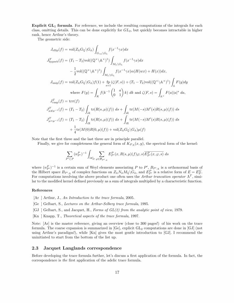
Explicit GL2 formula. For reference, we include the resulting computations of the integrals for eachclass, omitting details. This can be done explicitly for GL2, but quickly becomes intractable in higherrank, hence Arthur’s theory.

The geometric side:

Jellip(f) = vol(ZAGQ\GA)

∫GγA\GA

f(x−1γx)dx

JThyperb(f) = (T1 − T2)vol((Q×\A×)1)

∫MA\GA

f(x−1γx)dx

− 1

2vol((Q×\A×)1)

∫MA\GA

f(x−1γx)α(H(wx) +H(x))dx,

Junip(f) = vol(ZAGQ\GA)f(1) + fps=1

(ζ(F, s)) + (T1 − T2)vol((Q×\A×)1)

∫AF (y)dy

where F (y) =

∫K

f(k−1

(1 a0 1

)k) dk and ζ(F, s) =

∫A×

F (a)|a|s da,

JTcusp(f) = trπ(f)

JTµ6=µ−1(f) = (T1 − T2)

∫iR

tr(R(s, µ)(f)) ds+

∫iR

tr(M(−s)M ′(s)R(s, µ)(f)) ds

JTµ=µ−1(f) = (T1 − T2)

∫iR

tr(R(s, µ)(f)) ds+

∫iR

tr(M(−s)M ′(s)R(s, µ)(f)) ds

+1

4tr(M(0)R(0, µ)(f)) + vol(ZAGQ\GA)µ(f)

Note that the first three and the last three are in principle parallel.Finally, we give for completeness the general form of KP,χ(x, y), the spectral form of the kernel:∑

P ′⊂P(nPP ′)

−1

∫ia∗M

∑ϕ∈BP ′,χ

EPP ′(x,R(s, µ)(f)ϕ, s)EPP ′(x, ϕ, s) ds

where (nPP ′)−1 is a certain sum of Weyl elements associating P to P ′, BP ′,χ is a orthonormal basis of

the Hilbert space BP ′,χ of complex functions on ZANAMQ\GA, and EPP ′ is a relative form of E = EGP .For computations involving the above product one often uses the Arthur truncation operator ΛT , simi-lar to the modified kernel defined previously as a sum of integrals multiplied by a characteristic function.

References

[Ar ] Arthur, J., An Introduction to the trace formula, 2005.

[Ge ] Gelbart, S., Lectures on the Arthur-Selberg trace formula, 1995.

[GJ ] Gelbart, S., and Jacquet, H., Forms of GL(2) from the analytic point of view, 1979.

[Kn ] Knapp, T., Theoretical aspects of the trace formula, 1997.

Note: [Ar] is the master reference, giving an overview (close to 300 pages!) of his work on the traceformula. The coarse expansion is summarized in [Ge], explicit GL2 computations are done in [GJ] (notusing Arthur’s paradigm!), while [Kn] gives the most gentle introduction to [GJ]. I recommend theuninitiated to start from the bottom of the list up.

2.3 Jacquet Langlands correspondence

Before developing the trace formula further, let’s discuss a first application of the formula. In fact, thecorrespondence is the first application of the adelic trace formula.

17

Let G = GL2 and G′ = D×, where D is a quaternion algebra over Q with S the (finite) set of placeswhere G′ does not split. Then Gv ' G′v for all v 6∈ S. The Jacquet Langlands correspondence for GL2

is the following:

Theorem 2.3.1. There is a bijection between automorphic representations π′ of G′A with dim π′ > 1and cuspidal automorphic representations of GA, such that for all v 6∈ S, π ' π′v and for v ∈ S, π′v isirreducible admissible, πv is square-integrable mod center.

We outline the proof of the theorem as follows: we develop the trace formulas for G and G′, thencompare them by match orbital integrals to obtain a spectral identity. From the identity one deducescharacter relations, and characterizes the image of the map.

Simple trace formula. First note that the quotient ZAG′Q\G′A is compact, so for D× we have

already

trR′0(f ′)+∑µ2≡1

vol(ZAG′Q\G′A)µ(f ′) = vol(ZAG

′Q\G′A)f ′(1)+

∑γ

vol(ZAG′γ,Q\G′γ,A)

∫G′γ,A\G

′A

f ′(x−1γx) dx.

On the other hand, the same quotient for G is not compact, but we have the following simplification:

Proposition 2.3.2. Choose f =∏fv such that for at least two places of v the local hyperbolic integrals∫

Gv

fv(g−1

(a 00 1

)g) d×g

vanish. Then one has

trR0(f) +∑µ2≡1

vol(ZAGQ\GA)µ(f) = vol(ZA\GA)f(1) +∑ellip

Jo(f)

The hyperbolic integrals vanish immediately; the unipotent orbital integrals vanish under the aboveassumption, since∫

Gv

fv(g−1

(1 10 1

)g) dg = lim

a→1|1− a−1|

∫Gv

fv(g−1

(a 00 1

)g) dg.

Also, the spectral contributions trR(s, µ)(fv) vanish immediately while the tr(M(0)R(0, µ))(f) = 0since M(0) intertwines R(0, µ) with itself, hence acts by scalar.

Matching orbital integrals. We say fv in C∞c (Zv\Gv) matches f ′v in C∞c (Z ′v\G′v), written f ′v ∼ fv,if

1. fv(1) = f ′v(1).

2. The regular hyperbolic integrals vanish identically as above.

3. for corresponding tori Tv and T ′v,∫Tv\Gv

fv(g−1tg)dg =

∫T ′v\G′v

f ′v(g−1t′g)d′g

Comparison. Now one shows that for matching f and f ′,

trR0(f) = trR′0(f ′)

by comparing the three corresponding terms. In fact, expanding the sum, one can show for fixedunramified representations τv for each v 6∈ S,∑

π

∏v∈S

tr πv(fv) =∑π′

∏v∈S

tr π′v(f′v),

18

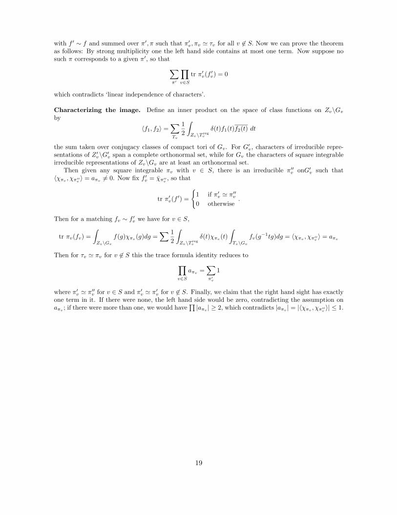
with f ′ ∼ f and summed over π′, π such that π′v, πv ' τv for all v 6∈ S. Now we can prove the theoremas follows: By strong multiplicity one the left hand side contains at most one term. Now suppose nosuch π corresponds to a given π′, so that∑

π′

∏v∈S

tr π′v(f′v) = 0

which contradicts ‘linear independence of characters’.

Characterizing the image. Define an inner product on the space of class functions on Zv\Gvby

〈f1, f2〉 =∑Tv

1

2

∫Zv\T reg

v

δ(t)f1(t)f2(t) dt

the sum taken over conjugacy classes of compact tori of Gv. For G′v, characters of irreducible repre-sentations of Z ′v\G′v span a complete orthonormal set, while for Gv the characters of square integrableirreducible representations of Zv\Gv are at least an orthonormal set.

Then given any square integrable πv with v ∈ S, there is an irreducible π′′v onG′v such that〈χπv , χπ′′v 〉 = aπv 6= 0. Now fix f ′v = χπ′′v , so that

tr π′v(f′) =

1 if π′v ' π′′v0 otherwise

.

Then for a matching fv ∼ f ′v we have for v ∈ S,

tr πv(fv) =

∫Zv\Gv

f(g)χπv (g)dg =∑ 1

2

∫Zv\T reg

v

δ(t)χπv (t)

∫Tv\Gv

fv(g−1tg)dg = 〈χπv , χπ′′v 〉 = aπv

Then for τv ' πv for v 6∈ S this the trace formula identity reduces to∏v∈S

aπv =∑π′v

1

where π′v ' π′′v for v ∈ S and π′v ' π′v for v 6∈ S. Finally, we claim that the right hand sight has exactlyone term in it. If there were none, the left hand side would be zero, contradicting the assumption onaπv ; if there were more than one, we would have

∏|aπv | ≥ 2, which contradicts |aπv | = |〈χπv , χπ′′v 〉| ≤ 1.

19

2.4 Refinement

The coarse expansion of the trace formula has two initial defects: first, its terms are often not explicitenough to use in applications and second, the distributions are generally not invariant under conjugation.To illustrate the importance of invariance we note that the Jacquet-Langlands correspondence in factinvolved the matching of invariant orbital integrals.

Given a Levi subgroup M in G, we denote by L(M) the set of Levi subgroups containing M , andP(M) the set of parabolic subgroups with Levi component M .

Weighted orbital integrals. There is a finite set So containing S∞ such that for any finite set Scontaining So and any f in C∞c (G1

FS),

Jo(f) =∑M∈L

|WM0 ||WG

0 |−1∑

γ∈(MF∩o)M,S

aM (S, γ)JM (γ, f)

where (MF ∩ o)M,S is the finite set of (M,S)-equivalence classes MF ∩ o and JM (γ, f) is the generalweighted orbital integral of f ,

JM (γ, f) = |D(γ)| 12∫Gγ(FS)\G(FS)

f(x−1γx)vM (x)dx

where vM (x) is the volume of the convex hull in aGM of th projection of points −HP (x)|P ⊃M fixedand D(γ) is the generalized Weyl discriminant∏

v∈Sdet(1−Ad(σv))g/gσv

where σv is the semisimple part of γv and gσv is the Lie algebra of Gσv .

Weighted characters. For any f in H(G),

Jχ(f) =∑M∈L

∑L∈L(M)

∑π

∑s

|WM0 ||WG

0 |−1|det(s−1)aGM |−1

∫ia∗M/ia

∗G

tr(ML(λ, P )MP (s, 0)Rπ(χ, λ)(f))dλ

where π runs over equivalence classes of irreducible unitary representations of M1A, s is a regular element

ofWL(M)reg = t ∈WL(M) : ker(t) = aL,

R is the induced representation IndGAPA

(σ⊗eλ(HP (·))) with matrix coeffecient π and χ = (P, σ), MP (s, 0)is the intertwining operator MQ|P (s, λ+ Λ) : HQ → HP with P = Q, and

ML(Λ, λ, P ) = MQ|P (λ)−1MQ|P (λ+ Λ)

(G,M) families. Arthur’s notion of (G,M) families unifies the computations required in refining bothsides. Suppose for each P ∈ P(M), cP (λ) is a smooth function on ia∗M . Then the collection cP (λ)is a (G,M)-family if cP (λ) = cP ′(λ) for adjacent P, P ′ and any λ in the hyperplane spanned by thecommon wall of the chambers of P and P ′.

For example, a collection of points XP in aM such that for adjacent P, P ′, XP −XP ′ is perpen-dicular to the hyperplane spanned by the common wall of the chambers gives a (G,M) family cP (λ) =eλ(XP ). In particular, XP = −HP (x) is such an orthogonal set, and we write vP (λ, xv) = e−λ(HP (xv)).

20

Now define a homogeneous polynomial θP (λ) = vol(aGM/Z(∆∨P ))−1∏α∈∆P

λ(α∨). Then we havethe

Lemma 2.4.1. For any (G,M) family cP (λ), the sum

cM (λ) =∑

P∈P(M)

cP (λ)θP (λ)−1

initially defined away from singular hyperplanes λ(α∨) = 0 extends to a smooth function on ia∗M .

In our example, vM can be shown to be the Fourier transform of the characteristic function of theconvex hull of XP . As a second example, dQ(Λ) = MQ|P (λ)−1MQ|P (s, λ′) with Λ = λ− λ′ is also aG,M)-family. It follows that (G,M)-families arise naturally as weight factors in the orbital integralsand characters, leading to a certain uniformity in the parallel refinements.

2.5 Invariance

Our strategy for making the fine trace formula invariant will be to subtract from weighted orbitalintegrals sums of weighted characters. In nice situations one can do this by applying Poisson summationto the distributions. We say that a continuous, invariant linear form I is supported on characters ifI(f) = 0 for any f ∈ H(GFS ) with fG = 0 as a complex function of tempered representations. If I issupported on characters, then there is a continuous linear form I on I(GFS ) such that I(fG) = I(f)

Now let Hac(GFS ) be the space of functions f on GFS with ‘almost compact support’, and define

φM (f) = JM (π,X, f) =

∫ia∗M,S/ia

∗G,S

JM (πλ, fZ)e−λ(X)dλ

where Z is the image of X in aG,S , fZ is the restriction of f to x ∈ GFS : HG(x) = Z and πλ is anorbit in Πunit(GFS ). In fact, φM : Hac(GFS )→ Iac(MFS ) is a continuous linear map.

Theorem 2.5.1. There exist invariant linear forms supported on characters

IM (γ, f) = JM (γ, f)−∑

L 6=G∈L(M)

ILM (γ, φL(f))

with γ ∈MFS , f ∈ Hac(GFS ) and

IM (π,X, f) = JM (π,X, f)−∑

L 6=G∈L(M)

ILM (π,X, φL(f))

with π ∈ Π(MFS ), X ∈ aM,S, f ∈ Hac(GFS ).

Then defining I(f) inductively by setting

I(f) = J(f)−∑

L6=G∈L(M)

|WM0 ||WG

0 |−1IL(φL(f)),

the (refined) invariant trace formula follows:

Theorem 2.5.2. For any f ∈ H(G) one has

I(f) = limS

∑M∈L

|WM0 ||WG

0 |−1∑

γ∈Γ(M)S

aM (γ)IM (γ, f) = limT

∑M∈L

|WM0 ||WG

0 |−1

∫Π(M)T

aM (π)IM (π, f)dπ.

where WG0 is the relative Weyl group, S is a finite set containing ramified places, Γ(M)S is the set

of (M,S)-equivalence classes, and dπ is a measure on Π(M)T , the union over 0 ≤ t ≤ T of Πt(M).

21

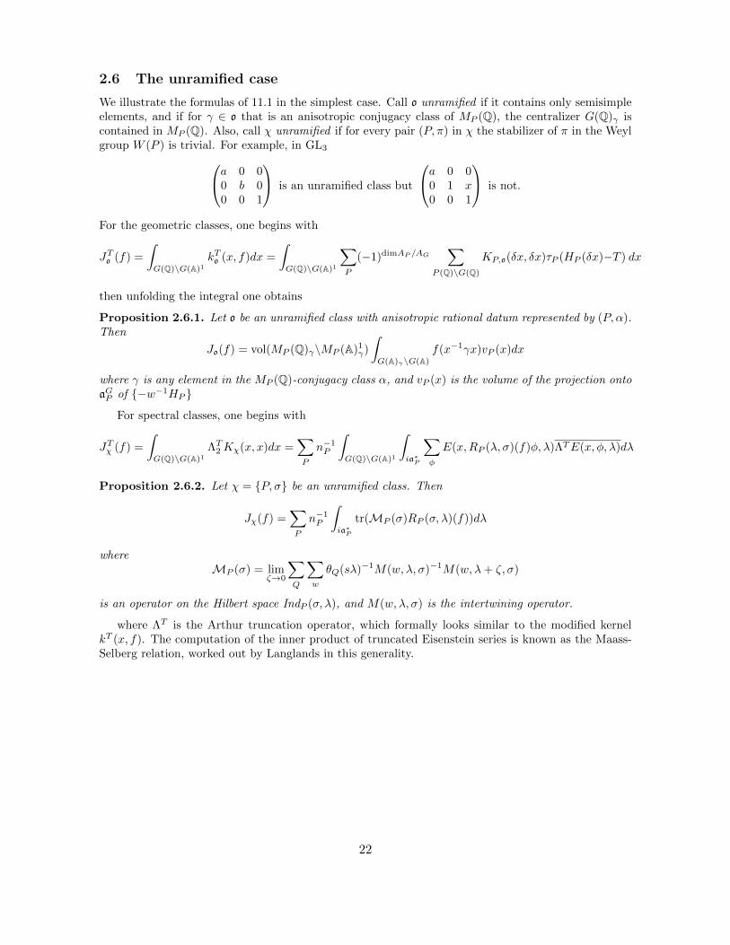
2.6 The unramified case

We illustrate the formulas of 11.1 in the simplest case. Call o unramified if it contains only semisimpleelements, and if for γ ∈ o that is an anisotropic conjugacy class of MP (Q), the centralizer G(Q)γ iscontained in MP (Q). Also, call χ unramified if for every pair (P, π) in χ the stabilizer of π in the Weylgroup W (P ) is trivial. For example, in GL3a 0 0

0 b 00 0 1

is an unramified class but

a 0 00 1 x0 0 1

is not.

For the geometric classes, one begins with

JTo (f) =

∫G(Q)\G(A)1

kTo (x, f)dx =

∫G(Q)\G(A)1

∑P

(−1)dimAP /AG∑

P (Q)\G(Q)

KP,o(δx, δx)τP (HP (δx)−T ) dx

then unfolding the integral one obtains

Proposition 2.6.1. Let o be an unramified class with anisotropic rational datum represented by (P, α).Then

Jo(f) = vol(MP (Q)γ\MP (A)1γ)

∫G(A)γ\G(A)

f(x−1γx)vP (x)dx

where γ is any element in the MP (Q)-conjugacy class α, and vP (x) is the volume of the projection ontoaGP of −w−1HP

For spectral classes, one begins with

JTχ (f) =

∫G(Q)\G(A)1

ΛT2 Kχ(x, x)dx =∑P

n−1P

∫G(Q)\G(A)1

∫ia∗P

∑φ

E(x,RP (λ, σ)(f)φ, λ)ΛTE(x, φ, λ)dλ

Proposition 2.6.2. Let χ = P, σ be an unramified class. Then

Jχ(f) =∑P

n−1P

∫ia∗P

tr(MP (σ)RP (σ, λ)(f))dλ

whereMP (σ) = lim

ζ→0

∑Q

∑w

θQ(sλ)−1M(w, λ, σ)−1M(w, λ+ ζ, σ)

is an operator on the Hilbert space IndP (σ, λ), and M(w, λ, σ) is the intertwining operator.

where ΛT is the Arthur truncation operator, which formally looks similar to the modified kernelkT (x, f). The computation of the inner product of truncated Eisenstein series is known as the Maass-Selberg relation, worked out by Langlands in this generality.

22

3 Base change

3.1 GL(2) base change

First let’s describe base change in general. Let G be a reductive groups over a number field F , andG′ = RE/FG the group obtained by restriction of scalars from a finite extension E/F . The RE/Ffunctor defines an isomorphism G′(F ) ' G(E). The principle of functoriality asserts that the diagonalembedding ϕ : LG→ LG′ should correspond to a lift of automorphic representations of G(F ) to G(E).

Langlands’ proof of base change for GL2 uses the invariant trace formula, and a twisted versionintroduced by Shintani. When G = GL2, then

LG = GL2(C)×Gal(k/k) and LG′ = (GL2(C)× · · · ×GL2(C)) o Gal(k/k)

with one copy of GL2 for each embedding of E into F , and Gal(k/k) acts by permuting the embeddings.We will work with E/F a cyclic extension of prime degree.

Conjugacy classes. Let E be a local field and F a cyclic extension of prime degree l. Gal(E/F ) :=ΓE/F acts on classes of irreducible representations of G(E) by Πσ(g) = Π(σ(g)). Fix a generator σ of

ΓE/F and define the norm N of g ∈ G(E) to be the intersection of the conjugacy class of gσ(g) . . . σl−1(g)with G(F ). If x = g−1yσ(g) for some g, x, y ∈ G(E), we say x and y are σ-conjugate.

Lemma 3.1.1. Now let F be a global field, and u ∈ G(F ). Then u = Nx has a solution in G(E) ifand only if it has a solution in G(Ev) for every v.

Spherical functions. Now let F be a nonarchimedean local field, and HF be the algebra of G(o)-bi-invariant functions on G(F ) with compact support mod NE/FZ(E), which transform by f(zg) =ξ−1(z)f(g) where ξ is a character of NE/FZ(E). Define HE similarly with Z(E) in place of NE/FZ(E).The map LG(F )→ LG(E) induces a homomorphism HE → HF .

Lemma 3.1.2. Suppose φ ∈ HE maps to f ∈ HF . If γ = Nδ then∫Gσδ (E)\G(E)

φ(g−1δσ(g))dg = ξ(γ)

∫Gγ(F )\G(F )

f(g−1γg)dg

where ξ(γ) = −1 if γ is central and δ is not σ-conjugate to a central element, and ξ(γ) = 1 otherwise.If γ ∈ G(F ) is not the norm of an element in G(E) then∫

Gγ(F )\G(F )

f(g−1γg)dg = 0.

Orbital integrals. Now let F be a local field of characteristic 0. Let f ∈ C∞c (G(F )) and γ ∈ Treg,a Cartan subgroup of G(F ), we define the following HCS family Φf (γ, T ) and Ψφ(γ, T ) Shintanifamily:

Φf (γ, T ) :=

∫T (F )\G(F )

f(g−1γg)dg; Ψφ(γ, T ) :=

∫Gσδ (E)\G(E)

φ(g−1δσ(g))dg

for all γ = Nδ, when there is no solution Ψφ(γ, T ) = 0. Now if γ = Nδ ∈ G(F ) then Gσδ (E) = Gσγ (F ),and we may use this to carry measures from Gγ(F ) to Gσδ (E), which is T (F ) for our choice of γ.

Lemma 3.1.3. A Shintani family is a HCS family. A HCS family is a Shintani family if and only ifΦf (γ, T ) = 0 when γ = Nδ has no solution.

Using this we may associate to any φ ∈ C∞c (GE) an f ∈ C∞c (GF ) such that Φf (γ, T ) =Ψφ(γ, T ). Note that f is not uniquely determined but its orbital integrals are, and we denote thecorrespondence φ → f. In particular, if E is unramified and φ = 1G(OE)vol(G(OE)) we can takef = 1G(OF )vol(G(OF )) by the homomorphism of Hecke algebras.

23

Comparison. Let r denote the representation of G(AF ) on the discrete spectrum of the space of func-tions on G(F )\G(AF ) that are square-integrable mod Z(F )NE/FZ(AE) and satisfy f(zg) = ξ(z)f(g),where ξ is a unitary character of NE/FZ(AE) trivial on Z(F ). Choose a a smooth, compactly supportedtest function f which at almost every place is Kv-invariant and supported on NEv/Fv (Z(Ev))Kv

Let R be the representation ofG(AE)×ΓE on the direct sum of τ and l copies of r. Here τ = 12⊕Sτ(η)

where S is the set of quadratic characters and τ(η) = τ(η, σ) = ρ(σ, ησ)M(η). If the degree of E/F isnot 2, then S is empty.

Suppose φ is as before. If v splits in E then φv is a product of l functions on G(Ev) ' G(Fv)×· · ·×G(Fv), and send φv = f1 × · · · × fl to f1 ∗ · · · ∗ fl. If v is not split in E, then map φv → fv followingLemma 11.3 if v is unramified and φv spherical or else Lemma 11.4.

Theorem 3.1.4. Let φ→ f as above. Then the trace identity tr(R(φ)R(σ)) = tr(r(f)) holds.

We omit the proof of this, but include the trace formula below for comparison by the reader usingthe matching outlined above. The only nontrivial portion proven using some functional analysis is∑

v

1

2π

∫s(η)=0

(lB(φv, ηv)−

∑η′→η

B(fv, η′v)) ∏w 6=v

tr(ρ(φ, ηw)ρ(σ, ηw))ds = 0

Further, one refines the identity to the following. Let V be a finite set including infinite and ramifiedplaces, and for v ∈ V fix an unramified representation Πv that lifts from πv and Πσ

v ' Π. Then oneshows: ∑

π

∏v∈V

trπv(fv) = l∑Π

∏v∈V

tr(Πv(φv)Π′v(σ)) +

∑(η,η)

∏v∈V

tr(τ(φv, ηv)τ(σ, ηv))

where π,Π, η are unramified outside of V , and (η, η) are such that η = (µ, ν) 6= η = ησ and µν = ξE .The Π sum has at most one term by strong multiplicity one, and by a different argument so does theη sum. In fact, one shows that one of the two sums must always be empty.

From this last identity, part of the main result obtained is the following

Theorem 3.1.5.Local results: every πv has a unique lifting Πv. Πv is a lifting if and only if Πσ

v ' Πv for all σ ∈ ΓEw/Fv .Local lifting is independent of choice of σ.

Global results: Every π has a unique lifting Π. If Π is cuspidal then it is a lifting if and only ifΠσ ' Π for all σ ∈ ΓE/F , furthermore, if Πv is a lift of πv for almost all v then Π is a lifting.

24

Trace formula. We introduce the trace formulas on the two groups without proof.

trf(f) =∑γ

ε(γ)vol(NE/FZ(AE)Gγ(F )\Gγ(AF ))

∫Gγ(AF )\G(AF )

f(g−1γg)dg (3.1)

− 1

4

∑ν=(µ,µ)

trM(η)ρ(f, η) (3.2)

1

4π

∫D0

m−1(η)m′(η)trρ(f, η)ds (3.3)∑a∈NE/FZ(E)\Z(F )

lλ0

∏v

L(1, 1Fv )−1

∫Gn(Fv)\G(Fv)

f(g−1ang)dg (3.4)

− lλ−1

∑v

∑a∈NE/FZ(E)\A(F )

A2(γ, fv)∏w 6=v

∆w(γ)

∫A(Fw)\G(Fw)

fw(g−1γg)dg (3.5)

1

2π

∫D0

∑v

B(fv, ηv)∏w 6=v

trρ(fw, ηw)ds (3.6)

Now the twisted formula:

trr(φ)r(σ) =∑

γ elliptic

ε(γ)vol(Z(AE)Gσγ (E)\Gσγ (AE))

∫Z(AE)Gσγ (AF )\G(AE)

φ(g−1γσ(g))dg (3.7)

∑γ central

ε(γ)vol(Z(AE)Gσγ (E)\Gσγ (AE))

∫Z(AE)Gσγ (AF )\G(AE)

φ(g−1γσ(g))dg (3.8)

1

4π

∫s(η)=0

m−1E (η)m′E(η)tr(ρ(φ, η)ρ(σ, η)) (3.9)

λ0Θ(0, φ) (3.10)

− λ−1

l

∑A1−σ(E)Z(E)\A(E)

∑v

A2(γ, φv)∏w 6=v

F (γ, φw) (3.11)

− 1

4

∑ησ=η

tr(ρ(φ, η)ρ(σ, ησ)M(η)) (3.12)

1

2π

∫s(η)=0

∑v

B(φv, ηv)∏w 6=v

tr(ρ(φ, ηw)ρ(σ, ηw))ds (3.13)

The matching is as follows: l[(7) + (8)] = (1), l(9) = (3), l(10) = (4), l(11) = (5), l(12) = (2) andl(13)− (6) remains.

The first terms, as always, are elliptic or central conjugacy classes. The terms containing m(η) orM(η), which are intertwining operators, are from the continuous spectrum. The terms containing λ0

and λ−1 are the first nonzero coefficients in the Laurent expansion of Tate’s zeta function at s = 1,coming from the unipotent classes. The surviving terms come from the hyperbolic classes, appearingas traces after applying Poisson summation to yield invariant distributions.

ReferencesLanglands, Base change for GL(2).

25

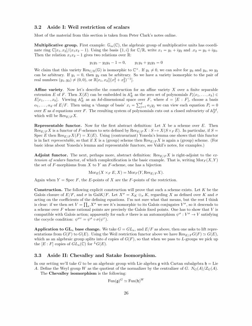
3.2 Aside I: Weil restriction of scalars

Most of the material from this section is taken from Peter Clark’s notes online.

Multiplicative group. First example: Gm(C), the algebraic group of multiplicative units has coordi-nate ring C[x1, x2]/(x1x2 − 1). Using the basis 1, i for C/R, write x1 = y1 + iy2 and .x2 = y3 + iy4.Then the relation x1x2 − 1 gives two relations over R:

y1y3 − y2y4 − 1 = 0, y1y4 + y2y3 = 0

We claim that this variety ResC/R(G) is isomorphic to C×. If y1 6= 0, we can solve for y3 and y4, so y2

can be arbitrary. If y1 = 0, then y2 can be arbitrary. So we have a variety isomorphic to the pair ofreal numbers (y1, y2) 6= (0, 0), or R[x1, x2][(x2

1 + x22)−1].

Affine variety. Now let’s describe the construction for an affine variety X over a finite separableextension E of F . Then X(E) can be embedded in AkE as the zero set of polynomials Pi(x1, . . . , xk) ∈E[x1, . . . , xk]. Viewing AkE as an kd-dimensional space over F , where d = [E : F ], choose a basis

α1, . . . , αd of E/F . Then using a ‘change of basis’ xi =∑dj=1 αjyj we can view each equation Pi = 0

over E as d equations over F . The resulting system of polynomials cuts out a closed subvariety of AkdF ,which will be ResE/FX.

Representable functor. Now for the first abstract definition: Let X be a scheme over E. ThenResE/FX is a functor of F -schemes to sets defined by ResE/FX : S 7→ X(S×F E). In particular, if S =Spec E then ResE/FX(F ) = X(E). Using (contravariant) Yoneda’s lemma one shows that this functoris in fact representable, so that if X is a (group) scheme then ResE/FX is again a (group) scheme. (Forbasic ideas about Yoneda’s lemma and representable functors, see Vakil’s notes, for examples.)

Adjoint functor. The next, perhaps more, abstract definition: ResE/FX is right-adjoint to the ex-tension of scalars functor, of which complexification is the basic example. That is, writing MorF (X,Y )the set of F -morphisms from X to Y an F -scheme, one has a bijection

MorE(X ×F E,X) = MorF (Y,ResE/FX).

Again when Y = Spec F , the E-points of X are the F -points of the restriction.

Construction. The following explicit construction will prove that such a scheme exists. Let K be theGalois closure of E/F , and σ in GalK/F . Let Xσ = XK ⊗σ K, regarding X as defined over K and σacting on the coefficients of the defining equations. I’m not sure what that means, but the rest I thinkis clear: if we then set V =

∏σX

σ we see it’s isomorphic to its Galois conjugates V σ, so it descends toa scheme over F whose rational points are precisely the Galois fixed points. One has to show that V iscompatible with Galois action; apparently for each σ there is an automorphism ψσ : V σ → V satisfyingthe cocycle condition: ψστ = ψσ σ(ψτ ).

Application to GLn base change. We take G = GLn, and E/F as above, then one asks to lift repre-sentations from G(F ) to G(E). Using the Weil restriction functor above we have ResE/FG(F ) ' G(E),which as an algebraic group splits into d copies of G(F ), so that when we pass to L-groups we pick upthe [E : F ] copies of GLn(C) for LG(E).

3.3 Aside II: Chevalley and Satake Isomorphism.

In our setting we’ll take G to be an algebraic group with Lie algebra g with Cartan subalgebra h = LieA. Define the Weyl group W as the quotient of the normalizer by the centralizer of G. NG(A)/ZG(A).

The Chevalley isomorphism is the following:

Fun(g)G ' Fun(h)W

26

where G acts on its Lie algebra by conjugation, so Fun(g)G denotes the functions on g invariant underconjugation by G. We may pass to the group setting:

Fun(G)G ' Fun(A)W , or C[G]G ' C[A]W

considering the group ring as conjugation-invariant complex valued functions on G.As reminder, the Satake isomorphism can be interpreted as:

H(G,K) ' C[A∨]W .

Where G is quasisplit. The Satake isomorphism has many incarnations, due to its successive general-izations. It starts life with the Satake transform giving an equivalence from the Hecke algebra of G withthat of the maximal torus/Cartan subgroup A, which then can be identified with the Hecke algebra ofthe maximal split torus T . Interpret the W -invariant functions on the tori as coming from the groupring of the character group, hence of the dual T∨.

Further, there is a grander geometric Satake equivalence, which gives an equivalence of certaintensor categories,

D-modules on the affine Grassmanian of G ' Representations of G∨ over C)

the most elegant proof of this equivalence is by Mirkovic-Vilonen, where C can be replaced by acommutative ring, using the Tannakian formalism.

Finally, our application to base change is the following: given a map of L-groups (specifically,an L-homomorphism) LG(F ) → LG(E) the Satake isomorphism induces a map of Hecke algebras atunramified places HEv → HFv , allowing for the transfer of spherical functions.

3.4 Aside III: Conjugacy classes in reductive groups

A regular element is one that has centralizer of minimal dimension. Ler’s look for the centralizerof an element of GLn. First, we invoke the rational canonical form over a field F : Given anendomorphism of x of V := Fn, V decomposes into a direct sum of cyclic submodules V1, · · · , Vd,where the minimal polynomials m(x, Vi) divides m(x, Vi+1). Moreover, m(x, V ) = m(x, Vd) and thecharacteristic polynomial c(x, V ) =

∏m(x, Vi).

An endomorphism of V commuting with x is a direct sum of homomorphisms between the Vi. Now Viis a quotient of Vj whenever i < j, so the dimension of homx(Vi, Vj) = min(dimVi,dimVj). When i > jone maps Vj into the unique cyclic submodule of Vi isomorphic to Vj , so homx(Vi, Vj) ' homx(Vi, Vi).Therefore the centralizer of x in End(V ) has dimension

d∑i,j=1

min(dimVi,dimVj) =

d∑i=1

(2d− 2i+ 1) dim(Vi)

because of the fact #(i, j)|1 ≤ i, j ≤ d and min(i, j) = k=2d-2k+1. So the dimension of the central-izer is at least the rank n of x, with equality if and only if m(x, V ) = c(x, V ). For x in Mn(F ) this isjust F [x]. For a semisimple matrix m(x, V ) = c(x, V ) means all its eigenvalues are distinct; while for aunipotent matrix this means it is similar to a Jordan block with 1 only on the diagonal or subdiagonal.

3.5 Noninvariant base change for GL(n)

Let γ, γ′ be in G(F ). We call γ and γ′ stably conjugate if they are conjugate in G(F ). For example,(cos θ − sin θsin θ cos θ

)=

(i 00 −i

)(cos θ sin θ− sin θ cos θ

)(−i 00 i

)shows two non-conjugate elements in SL2(R) that are conjugate over C.

27

Lemma 3.5.1. Two elements in G′(F ) := ResE/FGo θ are stably conjugate iff they are conjugate inG(E).

Let π, π′ be an admissible irreducible representations of G(F ), G′(F ), with character distributionsΘπ,Θπ′ . We say π′ is a base change of π if Θπ′(x) = e(G′)Θπ, where e is a certain Kottwitz constant.This is also called endoscopic correspondence.

Next, the following is known as endoscopic transfer over a local field: A pair of smooth, compactly-supported functions f and φ on G(F ) and G′(E) are called associated if for any regular γ in G(F ),

JG(γ, f) =∑δ

∆G′

G (γ, δ)JG′δ, φ).

where ∆G′

G (γ, δ) = 1 if γ is stably conjugate to δl and 0 otherwise, and δ runs over G(E)-conjugacyclasses in G′(F ). Then Labesse introduces a noninvariant version of association: f and φ are calledstrongly associated if for all Levis M and parabolics Q in G (resp. M ′, Q′ ∈ G′), one has

JQM (γ, f) = JQ′

M ′(δ, φ)

if γ ∈M(F ) is stably conjugate to δl ∈M ′(F ), and JQM (γ, f) = 0 if γ is not a norm.

Proposition 3.5.2. Let F be a local field, φ a smooth function on G′(F ) compactly supported on regularelements. Then there exists strongly associated φ′ and f ′ such that JG′(δ, φ) = JG′(δ, φ

′) for δ regularsemisimple. Conversely, given f with regular support, if JG(γ, f) = 0 if γ is not stably conjugate tosome δl ∈ G′(F ) then there exists strongly associated such that JG(γ, f) = JG(γ, f ′).

Then one proves a noninvariant fundamental lemma:

Theorem 3.5.3. Let F be a nonarchimidean local field, bE/F the base change homomorphism betweenunramified Hecke algebras. Then given h ∈ HE, hθ(xo θ) := h(x) and bE/F (h) are strongly associated.

To prove this we require the following base change identity:

Proposition 3.5.4. If φ on G′(AF ), f on G(AF ) are strongly associated and regular, then JQ′(φ) =

JQ(f).

RecallJQ′(φ) =

∑χ′

∑M

|WM0 ||W

Q0 |−1

∑L1,L2

dQM (L1, L2)JL′1,Q

′2

M ′,χ′ (φ)

where

JL1,Q2

M,χ′ (φ) =∑

π′∈Πdisc(M ′,χ′)

aM′

disc(π′)

∫ia∗M

rL′1M ′(π

′ΛE/F

)JQ′2M ′(π

′ΛE/FS

, φS)trπ′SΛE/F (hM ′) dΛ

Labesse’s main technical result is the refined base change identity:

Proposition 3.5.5. Assume normalizing factors are chosen to be compatible with weak base change.Let S be a finite set of places outside which E/F is unramified. Given a Levi M , a character ψ of theH(ASF ), if (fS , φS) are strongly associated regular functions, then

ldim aM∑

π′∈Πdisc(M ′)

δM′

M ′ (π′, ψ)aM

′

disc(π′)JQ′

M ′(π′, φS) =

∑π∈Πdisc(M)

δM′

M (π, ψ)aMdisc(π)JQM (π, fS)

where δG′

G (π, ψ) is 1 if tr πS(bE/F (h)) = tr ψ(h) and 0 otherwise; resp. tr π′S(h) = tr ψ(h) for

δG′

G′ (π′, ψ).

28

Starting from 12.4, assume inductively that 12.5 holds for proper parabolic subgroups of Q. Thenwe have

ldim aM∑

π′∈Πdisc(M ′)

δM′

M ′ (π′, ψ)aM

′

disc(π′)rL′1M ′(π

′)JQ′2M ′(π

′, φ) =∑

π∈Πdisc(M)

δM′

M (π, ψ)aMdisc(π)rL1

M (π′)JQ2

M (π, φ).

As in Langlands’ proof, we cancel terms and are left with the identity∑M

|WMo ||WG

0 |−1(∑

χ′

JM′,Q′

M ′,χ′ (φs ⊗ hθ)−∑χ

JM,QM,χ (fS ⊗ bE/F (h))

)= 0

From here one deduces the identity using ‘separation of infinitesimal characters via multipliers’ and thefundamental lemma above.

The trace identity in place, we also require the following rigidity result by Moeglin and Waldspurger:

Theorem 3.5.6. Let π1, π2 be cuspidal unitary automorphic representations of GLn, π the contragre-dient of π, and S a finite set containing the archimedean places and outside which the representationsare unramified. Then LS(s, π1× π2) is regular nonzero for Re(s) > 1, and at s = 1 it has a simple poleif π1 ' π2, otherwise it is regular and nonzero.

Using this one proves the second crucial ingredient:

Proposition 3.5.7. Let π1, π2 be discrete automorphic representations of G(AF ) and ψ a charac-ter of H(G′(ASF )), then δG

′

G (π1, ψ) = δG′

G (π2, ψ) = 1 if and only if there exists a character ξ ofM(AF )/NE/FM

′(AE).Let π′1, π

′2 be discrete automorphic representations of G(AE) and ψ a character of H(G′(ASF )), then

δG′

G′ (π′1, ψ) = δG

′

G′ (π′2, ψ) = 1 if and only if π′1 ' π′2.

The πi occur discretely, hence are parabolically induced from a tensor of mi Speh representationsSpeh(σi), where σi are unitary cuspidal representations of Mi = GL(di), and n = midiri. One is led to∏

ξ

LS(s, σ1 × π1 × ξ) =∏ξ

LS(s, σ1 × π2 × ξ)

where ξ runs over Grossencharacters of F×/NE/FE×. The previous theorem shows that the left has a

pole, and from this one deduces that π2 = π1 ⊗ ξ.Remark : LS(s, π1 × π2) is the Rankin-Selberg convolution L-function. Initially defined by Rankin

and Selberg as an convolution integral, it was later interpreted as an automorphic L-function. Atthe nonarchimedean unramified places we use the Satake isomorphism to write Lv(s, π1 × π2) =det(1− q−sv αvβv) where αv, βv are the semisimple LG-conjugacy classes corresponding to π1, π2. ThenLS(s, π1×, π2) is the product over all v 6∈ S of the Lv(s, π1 × π2).

Finally, we have the main theorem: Let δG′

G (π, π′) = 1 if π′v is the base change of πv and 0 otherwise.

Theorem 3.5.8. Let F be a global field and E a prime cyclic extension of F . (i) Given π′ ∈ Πdisc(G′)there is π ∈ Πdisc(G) such that δG

′

G (π, π′) = 1, unique up to twists by characters ξ. (ii) Given π ∈Πdisc(G) there is a unique π′ ∈ Πdisc(G′) such that δG

′

G (π, π′) = 1. (iii) π′ is a strict base change of π

if δG′

G (π, π′) = 1.

Let’s prove (i). Propositions 12.6 and 12.8 show that given π′ such that aG′

disc(π′) 6= 0, for S largeenough and strongly associated (fS , φS) we have

aG′

disc(π′)tr π′S(φS) =∑

π∈Πdisc(G)

δG′

G (π′, π)aGdisc(π)tr πS(fS).

We want to show a π exists with δG′

G (π′, pi) = 1 and aGdisc(π) 6= 0. It suffices to produce a stronglyassociated (fS , φS) such that tr π′S(φS) 6= 0. Let γ′ ∈ G′v be a regular semisimple element such thatthe Θπ′ 6= 0. Then using regular transfer (12.3) one constructs strongly associated (fv, φv) withtr π′v(φv) 6= 0 by taking φv with support in a small enough neighborhood of γ′ with JG′(γ

′, φv) nonzeroat γ′. Note finally that similar results are proved over local F .

29

3.6 Aside IV: L-group exercise

Let’s work through the construction of the L-group of GL3, over a base field k to start. A torus T is agroup isomorphic to copies of the multiplicative group scheme Gm. As is standard, we take the diagonalmatrices as our maximal torus

T =

∗ ∗∗

where indeed T ' G3

m over k, so T is a split torus. We have its character group X∗(T ) = Hom(T,Gm)and cocharacter group X∗(T ) = Hom(Gm, T ). Concretely, we have morphisms αi : T → Gm by theprojection αi(t) = ti, and the λ : Gm → T sending x to aii, for example:

λ2(x) =

1x

1

thus X∗(T ) =

⊕Zαi and X∗(T ) =

⊕Zλi for 1 ≤ i ≤ 3. Note that both are isomorphic to Z3.

The adjoint action of t ∈ T on the Lie algebra g = gl3, the group of 3× 3 matrices is

Ad(t)(aij) = t(aij)t−1 = (tit

−1j aij).

The generalized eigenvectors must then be the eij with aij = 1 and 0 elsewhere. i.e., Ad(t)eij = tit−1j eij

for any t in T . This corresponds to the character (αi − αj)(t)eij = tit−1j eij and we get to decompose

g =⊕i,j

gαi−αj =⊕i,j

〈eij〉.

The set of roots is Φ = αi − αj : i 6= j. Using the pairing 〈αi, λj〉 = δij we define for each root α thecoroot α∨ by condition 〈α, α∨〉 = 2. In our case, (αi−αj)∨ = (λi−λj). Finally we have the root datumof our reductive group, Ψ = (X∗(T ),Φ, X∗(T ),Φ∨). Inverting the datum Ψ = (X∗(T ),Φ∨, X∗(T ),Φ)this defines the dual torus T , and thus a dual reductive group G. Since the roots and coroots of GLnare isomorphic,

ˇGLn = GLn.

but more interestingly SLn and PGLn are dual, also SO2n+1 and Sp2n+1.We’re halfway to the L-group. Next we need a Galois action. From the action of Γ := Gal(k/k).

on k, we get an action of σ ∈ Γ on γ ∈Aut(G(k)) by σ(γ) = σγσ−1. Defining the 1-cocycle c : Γ →Aut(Gk) to be c(σ) = γ−1σ(γ), this satisfies the cocycle relation

c(σ1σ2) = c(σ1)σ1(c(σ2),

leading to the pointed set H1(Γ,Aut(Gk). But what we really want is an action of Γ on Aut(Ψ0), wherewe’ve chosen a basis for Φ. Given the Γ action on T ⊂ G, the character group X∗(T ) inherits the action

σ(α(t)) = σασ−1

where the first σ−1 acts on T , while the second σ acts on Gm.Implicitly we have made a choice a maximal torus T , which also fixes our choice of Borel subgroup

B (e.g., upper triangular matrices). It turns out that σ(γ) sends the B to another Borel, which beingdefined as the minimal parabolic we may conjugate it back to B. In fact, choosing the conjugatingelement g appropriately, we obtain an automorphism of Ψ0. So for ρ ∈ Aut(Ψ0) we set σ(ρ) =Inn(g)σρσ−1.

[Not relevant : It turns out that Γ preserves inner automorphisms, so the exact sequence holds:

0→ Inn(G)→ Aut(G)→ Aut(Ψ0)→ 0

30

Considering the group GL2(R), its based root datum is (Z2, (1,−1),Z2, (1,−1)). Then we have

0→ PGL2(C)→ Aut(GL2(C))→ ±1 → 0.]

Also note that if G is split over k, the above discussion shows that Γ must act trivially on Gk. Finally,we define the L-group of G over k to be the semidirect product with the complex group

LG := G(C) o Gal(k/k).

In particular, since GL3 is split since it contains our split torus T , so LGL3 = GLn(C)×Gal(k/k).Now for the restriction of scalars ResE/FG, where E is some field extension of F . Let’s work our way

up. From 12.4, we showed ResC/RGm ' C×, which over R is R[x, y, z] with the relation z(x2 + y2) = 1.I think because we can vary the two factors we obtain the maximal torus T (R) ' (R×)2. Then lookingat X∗(T ) the two roots are identical, inverting the root datum we find T ' G2

m, which is our dualgroup already.

LResC/RGm(R) = (Gm(C)×Gm(C)) o Gal(C/R).

The Galois action on C exchanges 1 with i, so on X∗(T ) it exchanges to two roots, and on T it permutesthe Gm factors. (In general, given a separable extension E/F , L×F F ' F × · · · × F.)

From this and the exercise on affine varieties it we might believe that over F ,

LGL3(E) = (GL3(C)× · · · ×GL3(C)) o Gal(E/F )

where the number of copies is [E : F ], or the number of embeddings of E into F , and Gal(E/F ) acts bypermuting the factors. This construction supposedly holds for the restriction of any algebraic group.As a reminder, the pertinent application here is that the base change map of L-groups induces a mapof Hecke algebras by the Satake isomorphism.

References[Bu] Buzzard’s online notes (Forms of reductive algebraic groups).[La] Labesse, Noninvariant base change identities, 1995.[Ma] Makisumi, Structure Theory of Reductive Groups through Examples.[Sa] Sakellaridis’ course notes (Lecture 2: Structure and forms over a non-algebraically closed field).

4 Endoscopy theory

4.1 Warmup on group cohomology

Let Γ be a group acting on a set G, denoted σ(g) or σg. The zeroth cohomology is the fixed point set

H0(Γ, G) := GΓ = g ∈ G : σ(g) = g for all σ ∈ Γ.

Now let G be a group. A map c : Γ→ G is a 1-cocycle if c(σ1σ2) = c(σ1)σ1(c(σ2)) holds for any σ1, σ2.Call two 1-cocyles c1, c2 equivalent if c2(σ) = g−1c1(σ)σ(g) holds for some g in G. Then we define

H1(Γ, G) := 1-cocycles c : Γ→ G/ ∼

In the general setting the cohomology groups are defined functorially, which we’ll not discuss here.Given a homomorphism f : H → G of groups with Γ actions, the map of cocycles cb(σ) = f(ca(σ))

induces a map H1(Γ, H)→ H1(Γ, G). If H and G are abelian then it’s a group homomorphism, if notthen H1 is not a group in general, but we have a distinguished class g−1σ(g), which allows us to definethe kernel of the given map.

Now let G be a connected linear algebraic group with a homomorphism f : G→ H. We say (G, f)is a cover of H if f is onto with finite kernel. We also call G simply connected if it is connected andevery cover of it is an isomorphism. Third, the derived subgroup Gder is the largest normal subgroupsuch that G/Gder is abelian.

31

4.2 Endoscopic character

Let G be a reductive group over a characteristic 0 field k, Gsc the simply connected cover of Gder. Givenγ in Gk, denote Iγ the centralizer of γ (Labesse uses the subgroup in G generated by Z(G) and theimage in G of the centralizer of γ in Gsc). In particular, if γ is regular semisimple then Iγ is a torus.

Suppose γ, γ′ in Gk are regular semisimple and stably conjugate, then for a g in Gk and any σ inΓk,

γ′ = σ(γ′) = σ(gγg−1) = σ(g)γσ(g)−1 = σ(g)g−1γ′gσ(g)−1 = c(g)−1γ′c(g)

That is, c(g) = gσ(g)−1 defines a 1-cocycle in H1(k, T ), trivial in H1(k,G). Also from the long exactsequence on cohomology induced by 1→ T → G→ T\G→ 1 we have

H0(k, T\G)→ H1(k, T )→ H1(k,G).

One checks that γ 7→ c defines a bijection from Gk-conjugacy classes in the stable conjugacy class of δto

D(k, T ) := ker(H1(k, T )→ H1(k,G))

So we see that Iγ\G(k) = H0(k, T\G) is the stable class of γ by the exact sequence

1→ T (k)\G(k)→ T\G(k)→ D(k, T )→ 1.

Where the left are naturally conjugacy classes of γ, and the right parametrizes conjugacy classes in thestable class. From abelianized cohomology (taken on faith) one also has a long exact sequence

· · · → H0ab(k,G)→ H1(k,Gsc)→ H1(k,G)→ H1

ab(k,G)

which gives an injection

D(k, T ) → E(k, T ) := ker(H1(k, T )→ H1ab(k,G)) = im(H1(k, Tsc)→ H1(k, T )).

When k is nonarchimedean local, H1(k,Gsc) = 1 (Kneser) and in fact it is a bijection. Note D(k, T )is in general only a set, but it turns out that E(k, T ) is abelian, and finite for k local. Then by thecomposition

H0(k, T\G)→ D(k, T ) → E(k, T ),

a character κ of E(k, T ) defines a character on H0(k, T\G), called endoscopic characters. By Tate-Nakayama duality below this will give us the endoscopic group, and also define the κ-orbital integralsbelow.

4.3 Rational representative

First we need a black box: Let T be a torus over a local field k and split over a Galois extension k′.

Theorem 4.3.1. (Tate-Nakayama duality) There is a canonical isomorphism of Tate cohomologygroups

Hi(k′/k,X∗(T ))→ H2+i(k′/k, Tk)

This is a result of local class field theory. In particular, we have an isomorphism

H−1(k′/k,X∗) := H0(Γ, X∗) = XNΓ∗ /IΓX∗ → H1(k′/k, Tk) = H1(k, T )

where XNΓ∗ is the kernel of x 7→

∑σ(x) and IΓ the augmentation ideal IΓ :=

∑nσσ :

∑nσ = 0 ⊂

Z[Γ], all sums over Γ.Here is a retelling: let G be a reductive group over k and Z(G) the center of its complex dual group.

Tate-Nakayama gives a canonical isomorphism from Galois cohomology to the character group

H1(k,G)→ π0(Z(G)Γ)∗.

32

The important point is that an endoscopic character will correspond to an element of G.Let k be a global field. Combining the above with the long exact sequence of cohomology (via the

derived functor etc.) for the exact sequence 1→ Tk → TAk → TAk/Tk and the isomorphism

H1(k, TAk) '⊕v

H1(kv, T )

(by Shapiro’s lemma etc.), we can measure the obstruction to a strongly regular semisimple GA-conjugacy class γ having a rational representative γv for every v by

coker(H1(k, T →⊕v

H1(kv, T )) ' im(⊕v

π0(TΓv )∗ → π0(TΓ)∗)

There is a similar picture for Tsc involving E(k, T ) ⊂ H1(k, T ), and replacing π0(TΓ) with the groupK(k, T ) ⊂ π0((T /Z(G))Γ) whose image in H1(kv, Z(G)) is trivial for all v.

Langlands’ idea was to use Fourier transform on the finite cokernel so that the part of the traceformula corresponding to the stable class γ becomes a sum over characters, where the trivial characterdefines the stable part of the trace formula, the rest a product of κ-orbital integrals.

4.4 Endoscopic group

Start with T = Iγ , κ an endoscopic character. Let s be the image of κ in G, and H = Gs its connectedcentralizer in G. Then inverting the roots one obtains the endoscopic group H associated to κ. Ingeneral H may not be a subgroup of G, which we will now discuss.

Fixing an embedding of the Weil form of LT → LG = GoWk, we have an L-subgroup Gs = LTGs,

1→ Gs → Gs →Wk → 1

a split extension of Wk, acting on Gs by outer automorphisms, and let Gs be a quasisplit group over kdual to Gs. It contains a maximal torus Ts = Gδ′ , with δ, δ′ related by an isomorphism of T, Ts. Wehave

(δ, κ)→ (Gs,Gs, s, δ′),

a correspondence motivating the definition of endoscopic datum (Gs,Gs, s, ξ) for a reductive group G,where Gs is a quasisplit group over k, the endoscopic group; Gs a split extension of Wk by Gs; ssemisimple in G; ξ an embedding of Gs in LG such that ξ(Gs) is the connected centralizer of s in Gand ξ(u)s = sξ(u)a(u), for u ∈ Gs, and a a locally trivial 1-cocycle from Wk to Z(G). This is so that ξextends to an L-homomorphism.

Example 4.4.1. The centralizer of any semisimple s in GLn is a product of GLni , so its endoscopicdatum is represented by a Levi M , and the only datum where im(ξ) is not contained in a proper Levi isGLn itself. For other classical groups like Sp(2n), its endoscopic groups are of the form Sp(2n− 2k)×Sp(2k).

Once again, the endoscopic group Gs is not a subgroup of G in general. Nevertheless we can stilltransfer stable conjugacy classes. Assume for simplicity that Gs is split, so the inclusion Gs ⊂ G inducesan inclusion of Weyl groups Ws ⊂ W , and there is a canonical map t/Ws → t/W . If γs in gs(k) hascharacteristic polynomial as ∈ t/Ws(k) mapping to the characteristic polynomial a of γ in G(k), wewill say the stable class of γs transfers to to the stable class of γ.

The Kostant section is a section of the characteristic polynomial morphism g→ t/W , distinguishinga conjugacy class by a stable class a in t/W (k). The section helps define the transfer factor.

33

4.5 Stable distributions

Let’s first motivate the problem, leaving precise definitions for later. Let k be a local field. Denote∆reg(Gk) the set of strongly regular stable conjugacy classes, and let δ be such a class. Given fv ∈C∞c (Gv), a stable orbital integral is

SOδ(fv) =∑γ∼δ

Oγ(fv) =∑γ∼δ

∫Iγ(kv)\Gv

fv(g−1γg)dg,

a finite sum over conjugacy classes in the stable class of δ; and aslo the κ-orbital integral

Oκδ (fv) =

∑γ∼δ

κ(γ)Oγ(fv).

One difficulty here is that κ(γ) depends on the choice of representative δ; to correct this the Langlands-Shelstad transfer factor ∆(γ, δ) was introduced, depending only on the classes of δ and γ. Second, theglobal stable class δA is a product of local rational representatives, so we need each ordinary class γAto also have a rational representative. We will measure the obstruction to this cohomologically.

An invariant distribution on Gv is a stable distribution if its value at fv depends only on the stableorbital integrals SOδ(fv), i.e., it belongs to the closure of the space spanned by SOδ(fv). The termsin the invariant trace formula are not stable, and the aim here is to stabilize the trace formula.

Theorem 4.5.1. Let H be an endoscopic group of a reductive group G. Then

1. (Transfer) For every f ∈ C∞c (Gk) there exists a fH ∈ C∞c (Hk) such that

SOγH (fH) = ∆(γH , γ)Oκγ(f) (∗)

for all γH , γ strongly regular semisimple with characteristic polynomial of γH mapping to that ofγ.

2. (Fundamental lemma) (*) holds for f = 1g(Ok) and fH = 1h(Ok).

3. (*) holds for any f ∈ HG and fH = b(f) ∈ HH , where b is induced from the map of L-groups.

Langlands and Shelstad proved this for archimedean k around 1987. The nonarchimedean casewaited another thirty years for the work of Laumon, Waldspurger, Ngo, and many others, completedin 2008.

References[Ar] Arthur, An introduction to the trace formula[La] Labesse, Introduction to endoscopy[Ng] Ngo, Endoscopy theory of automorphic forms

34

5 Fundamental lemma

The fundamental lemma, initially arising in the theory of endoscopy, is a broader phenomenon. Soone may speak of ‘fundamental lemmas’. We will not be able to treat the fundamental lemma in anycompleteness, but I will introduce the main objects and the broad outline of its proof. But first let’sreview the statement of the lemma.

Let G be a reductive group over a local field Fv. Given an element γ in G, denote Iγ(Fv) itscentralizer in G. Define the orbital integral of a smooth compactly supported function fv on G(Fv):

Oγ(f) :=

∫Iγ(Fv)\G(Fv)

fv(g−1γg)dg.

A character κ of Iγ defines a subgroup H of G, called the endoscopic subgroup. We say γH ∈ H andγ ∈ G correspond if their characteristic polynomials are equal. Also, call two elements γ and γ′ in Gstably conjugate if they are conjugate over Fv. The transfer conjecture states that

Conjecture 5.0.1. For every fv ∈ C∞c (G(Fv)) there exists an fHv ∈ C∞c (H(Fv)) such that

(f) :=∑γH

OγH (fHv ) = ∆(γH , γ)∑γ

κ(γ)Oγ(fv) (∗)

for all strongly regular semisimple γH , γ with equal characteristic polynomial, and the sums taken overstable conjugacy classes. ∆(γH , γ) is called the transfer factor (which we won’t define).

The left is called a stable orbital integral SOγH and the summands on the right are κ-orbital integralsOκγ . The fundamental lemma asserts that the identity (*) holds for fv, f

Hv chosen to be the unit

elements 1G(Ov), 1H(Ov) of the respective Hecke algebras.

5.1 Transfer to characteristic p

The series of reductions are as follows:

1. Waldspurger: The fundamental lemma (FL) implies the transfer conjecture.

2. Hales: FL for units at almost all v implies the FL for Hecke algebra at all v.

3. Waldspurger, Hales: Lie algebra FL implies Lie group FL.

4. Waldspurger, Cluckers-Hales-Loeser: FL for local fields of char p implies FL for char 0.

What is finally proven is the following:

Theorem 5.1.1. (Ngo) Let k = Fq, Fv its field of fractions k((π)) and Ov = k[[π]]. Let G be a reductivegroup scheme over OF where the order of its Weyl group does is not divisible by char(k). Let H be anendoscopic group of G defined by the character κ and L-embedding ξ. Let a and aH be correspondingstable semisimple conjugacy classes. Then there is an identity of κ-orbital integrals and stable orbitalintegral:

∆G(a)Oκa(1g(OF )) = ∆H(aH)Oκ

aH (1h(OF ))

where ∆G and ∆H are transfer factors, and are powers of q.

The proof ingredients were developed as follows:

1. Goresky-Kottwitz-MacPherson: Local method using equivariant cohomology of Khazdan-Lusztig’saffine Springer fibers.

2. Ngo: Global method using perverse sheaves in cohomology of Hitchin fibration.

3. Laumon and Ngo: Proved FL for unitary groups, followed by Ngo for all reductive groups.

This is the journey we shall now describe. Let’s set the stage: unless otherwise stated, fix X a smooth,geometrically connected, projective curve of genus g over a finite field k, and X = X ×k k. Denote Fthe function field of X, Fv the fraction field of the completed local ring at a closed point v in X, Ovits ring of integers, and kv the residual field.

35

5.2 A first example: SO5 and Sp4

Let Fv be a nonarchimedean local field with residue field k with q > 2 elements. Let 0,±t1,±t2 be theeigenvalues of an element γ in so(5) and assume there is an odd r such that |α(γ)| = q−r/2 for everyroot α of so(5). Using the eigenvalues Hales constructs the elliptic curve Ea over k given by

y2 = (1− x2τ1)(1− x2τ2)

where τi is the image of t2i /$r in the residue field. By direct calculation he shows that the stable orbital

integral of f at γ is equal to the number of points on the elliptic curve up to rational functions A andB,

SOγ(f) = A(q) +B(q)|Eγ(k)|

Next with sp(4), there is an element a′ with eigenvalues ±t1,±t2. (Twisted) endoscopy predicts an f ′

on sp(4) with stable orbital integral equal to that of f . But calculating the integral of f ′ gives a similarformula with another elliptic curve E′γ′ , having different j-invariant. The desired equality is obtainedby producing an isogeny between Eγ and E′γ′ . As we shall see, these elliptic curves are ‘spectral curves’.

5.3 Examples of GLn Hitchin fibres

Now let k = Fq and consider P1k = Speck[y] ∩ 0. Fix the divisor D = 2[0], the total space of the line

bundle OP1k(D) is

Spec(

∞⊕i=0

OP1k(−iD)ti)→ P1

k.

Define the scheme A classifying characteristic polynomials t2 − a1(y)t− a2(y) where for i = 1, 2,

ai(y) ∈ H0(P1k,O(iD)) = ai(y) ∈ k[y] : deg(ai) ≤ 2i

such that the discriminant a21 − 4a2 is non vanishing at y = 0. The spectral curve Ya is the preimage

of t2 − a1(0)t− a2(0) in the total space. Assume further that a1 = 0. The following cases hold:

1. a2 has only distinct roots. Then Ya is a smooth projective curve of genus one, i.e., an ellipticcurve.

2. a2 has a double root and two distinct roots. Then Ya is integral and its only singularity is a node.

3. a2 has a triple root. Then Ya is integral and its only singularity is a cusp.

4. a2 is a square of a polynomial with two distinct roots. Then Ya has two irreducible componentswhich intersect transversally.

The Hitchin fibres, defined below, can be identified with the compactified Jacobians of each Ya.

5.4 An extended example: GLn

Though stability is trivial for G = GLn since stable conjugacy is the same as ordinary conjugacy, thegeometric constructions on GLn as a prototype will give us intuition for arbitrary reductive groups.

5.4.1. Chevalley characteristic and Kostant section. Consider the Lie algebra g = gln. Fix aCartan subalgebra t of diagonal matrices and Weyl group W = Sn. By Chevalley, the adjoint action ofG on g (i.e., conjugation) induces an isomorphism

k[g]G∼−→ k[t]W

Let c := Spec(k[t]W ) is the affine space of degree n monic polynomials, isomorphic to An by

pA := Xn − a1Xn−1 + · · ·+ (−1)nan 7→ (a1, . . . , an).

36

The Chevalley characteristic χ : g → c sends A to its characteristic polynomial det(XI − A), orequivalently,

χ : A 7→ a = (tr(A), tr(∧2A), . . . , tr(∧nA)).

The Kostant section ε of the map χ constructs a matrix with the given characteristic polynomial. Thecompanion matrix obtained by the endomorphism X of R := k[X]/(pA)

ε : (a1, . . . , an) 7→

0 . . . 0 (−1)n−1an

1. . .

... (−1)n−2an−1

.... . . 0

...0 . . . 1 a1

.

The Kostant section is a similar but different from the companion matrix which generalizes to reductivegroups.

The centralizer of a companion matrix can be identified with the centralizer of X in GL(R), andone checks that

Ja ' R× ⊂ GL(R) and Iγ ' R ⊂ gl(R).

More generally, if two regular elements in g have the same characteristic polynomial a, then theircentralizers are canonically isomorphic. Also, for every a there is a regular centralizer Ja isomorphic toIγ for any γ such that χ(γ) = a.

5.4.2. Affine Springer fibre. Now for the affine setting. Define the affine Grassmannian

Gr := G(Fv)/G(Ov) = Ov-modules of rank n, i.e., lattices in Fnv ,

where we deduce the latter from G(Fv) acting transitively on lattices with G(Ov) fixing Ov-lattices.Given a Kostant section ε(a) = γ, consider the following subset of g×G(Fv)/G(Ov),

g(Fv) = (γ, g) : Ad(g)−1(γ) ∈ g(Ov)).

The fibres of its projection to the first factor π : g(Fv)→ g(Fv) are called the affine Springer fibres,

Mv(a) := π−1(γ) = g ∈ G(Fv)/G(Ov) : Ad(g)−1(γ) ∈ g(Ov)).

Now the standard lattice Λ0 := Onv is γ-stable if and only if γ ∈ g(Ov). Given another latticeΛ = gΛ0, Λ is γ-stable if and only if L0 is g−1γg-stable if and only if Ad(g)−1(γ) ∈ g(Ov)). Thus theaffine Springer fibre parametrizes γ-stable lattices. One also writes

Grγ :=Mv(a) = Ov-modules Λ of rank n in Fnv : γ(Λ) ⊂ Λ.

5.4.3. Local orbital integrals. Let γ be a regular semisimple element. Its centralizer Iγ is a torusTFv . We want to count γ-stable lattices in Fnv modulo the action of TFv . Any element of T fixes γ, sothe action preserves the fiber Grγ . Restricting to the subgroup X∗(T ), the stabilizer of a lattice is acompact discrete subgroup hence a finite group, which must be trivial since X∗(T ) is a free Z-module.So X∗(T ) acts freely. Now

Oγ(1g(Ov)) =

∫X∗(T )\GF

1g(Ov)(x−1γx)dx =

∑X∗(T )\GF /GOv

∫GOv

1g(Ov)(k−1x−1γxk)dk

setting vol(G(Ov)) = 1,

=∑

X∗(T )\GF /GOv

1g(Ov)(x−1γx) = |X∗(T )\Grγ |

Thus local orbital integrals are equivalent to counting points on the affine Springer fibre modulo theaction of the group

Pv(a, k) = Ja(Fv)/Ja(Ov) ' Iε(a)(Fv)/Iε(a)(Ov).

37

5.4.4. As stacks. Schemes can be seen, by the functor of points Hom(−,M), as sheaves of sets onthe category of (Sch/S) with the etale topology. A stack, by contrast, is a sheaf of groupoids, where agroupoid is a category in which every morphism has an inverse.

The affine Springer fibre represents the functor from schemes to groupoids

Mv(a) : S 7→

E, rank n vector bundles on Spec(Ov)× S with

γ, a section of E over Spec(Ov)× Sι, a trivialization of E over Spec(Fv)× S

(the affine Grassmannian is similarly defined, without the second datum) while the Picard stack repre-sents

Pv(a) : S 7→

F, Ja-torsors on Spec(Ov)× Sι, a trivialisation of F over Spec(Fv)× S

In particular, Pv(a, k) ' Ja(Fv)/Ja(Ov) ' Iε(a)(Fv)/Iε(a)(Ov).The corresponding global object is the Hitchin stack associating to schemes the groupoids:

M : S 7→

E, rank n vector bundles on X × S with

φ, a twisted endomorphism E → E ⊗OX(D)

where D is an even, effective divisor on X, and (E, φ) is called a Higgs pair. One also has a Picardstack

P : S 7→Ja-torsors on X × S for every a in A

where the scheme A is the Hitchin base over which the Hitchin stack fibers, which we next introduce.

5.4.5. Hitchin fibration. The Hitchin fibration is the morphism f :M→A sending a pair

(E, φ) 7→ (tr(φ), tr(∧2φ), . . . , tr(∧nφ))

where tr(∧iφ) is the trace of the endomorphism ∧iφ : ∧iE → ∧iE ⊗OX(iD). The fibers Ma := f1(a)of the map will be the global analogue of the affine Springer fibres.

The Hitchin base A is the affine space of characteristic polynomials,

Xn − tr(φ)Xn−1 + · · ·+ (−1)ntr(∧nφ)

identified with the space of global sections of X × S with values in cD := c⊗OX OX(D)

A =⊕

1≤i≤n

H0(X,OX(iD))

Define (Aani and) A♥to be the subset of A(k) corresponding to the (anisotropic) regular semisimplesubset of c. These are open subschemas of A. Define similarly M♥ and Mani by pulling back along f .

5.4.6. Global orbital integrals. Attach to the divisor D =∑v∈|X| nv[v] an idele $D := ($nv

v ).

Then the degree morphism deg: A×F → Z which is trivial on F× and O× gives deg($D) = deg(D). Let

Ha := (g, γ) ∈ GA/GO × gF : deg(det(g)) = 0, χ(γ) = a, and g−1ag ∈ $−1D g(O)

Define a GF -action by left multiplication and conjugation respectively, forming the quotient stack[GF \Ha].

38

Let (γv) = $Dγ ∈ gA. The third (integrality) condition is equivalent to g−1v γvgv ∈ g(Ov) for all v,

and this coset is exactly the affine Springer fibre Grγv . Choosing a to be regular semisimple, the Hitchinfibre is

Ma(k) ' [GF \Ha] = [TF \Ha] = [TF \′∏

v∈|X|

Grγv ](k).

If we normalize measures so that vol(GOv ) = vol(TOv ) = 1 and define T 0A to be the elements of degree

0, then

|Ma|(k) = vol(TF \T 0A)∏∫

Tv\Gv1g(Ov)(g

−1v γvgv)dgv.

The expression is finite if and only if the Hitchin fiber has finitely many k-rational points. Also, γv is ing(Ov) for almost all v, so the orbital integral is almost always 1. At other places, the integral is takenover a compact subset (the conjugacy class of a semisimple element is closed) hence finite.

5.4.7. Spectral curve of X. Consider the total space of the line bundle OX(D)

ΣD =

∞⊕i=1

OX(−iD).

Given a k-point a of A, we have the characteristic polynomial pa : ΣD → ΣnD

pa(X) = Xn + a1(v)Xn−1 + · · ·+ an(v) = 0, ai ∈ H0(X,OX(iD))

The spectral curve Ya is the preimage under pa of the zero section of ΣnD, tracing out a closed curvein ΣD defined by pa(X) = 0. It is a n-fold finite cover of X, generically etale Galois of Galois groupW = Sn.

Related to this is the cameral cover X → X obtained by pulling back a Higgs pair along the fiberproduct g→ g of the quotient map t→ t/W and χ : g→ t/W . (Not quite sure how this works.)

5.4.8. Picard stack. The Beauville-Narasimhan-Ramanan correspondence states that when a is reg-ular, Ma is isomorphic to the moduli stack of coherent torsion-free sheaves F of generic rank 1 on Yawith a certain trivialization. When X is a curve this is the compactified Jacobian. In general,

Ma ' Pic0(Ya).

where Pic0(Ya) is the neutral component of the Picard scheme: the smooth commutative group schemeof degree 0 line bundles on Ya. When Ya is smooth these are just line bundles, and Ma is just theJacobian. The group of symmetries Pa can be identified with the Pic(Ya) acting on Ma by tensoringsheaves.

Now let a : X → cD be a point in A♥(k). Consider the normalization of the spectral curveξ : Y [a → Ya, and the pullback

ξ∗ : PicYa → PicY [a

The exact sequence0→ O×Ya → ξ∗O×Y [a → ξ∗O×Y [a /O

×Ya→ 0

implies ξ∗ is surjective on k-points, whose kernel consists of invertible sheaves on Ya that pullback tothe trivial bundle on Y [a . Define the Serre invariant of a normalization A of A, δA := length(A/A), inthis case

δa =∑y∈Ya

δOYa,y= dimH0(Ya, ξ∗O×Y [a /O

×Ya

) = dim ker ξ∗.

Also, the connected components π0(PicY [a ) ' Zπ0(PicY [a ).

39

5.4.9. Subschemes of A. Let’s describe some important subschemes of A:

1. A♥: The functor

B : S 7→

a : S → A♥, an S point of A♥

ξ : Y [a → Ya, a normalization of the spectral curve Ya.

is representable by a finite type k-scheme. The forgetful functor B → A♥ is a bijection on thelevel of k-points.

2. Aδ: The locally closed subset of a in A such that δa = δ, for fixed δ ∈ N. When δ = 0, we haveA0 = Asm, the open dense subset of a in A such that Ya is smooth. Denote Ψ the finite set ofconnected components of B, giving a stratification A♥ ×k k =

⊔ΨAψ. The invariants δa and

π0(Y [a ) are constant on each stratum. We may group together strata with equal δa,

Aδ =⊔

δ(ψ)=δ

Aψ.

3. Agood: The open set of all strata Aδ of codimension ≥ δ, and call its complement Abad. Notethat this condition fails outside the anisotropic set, hence Agood ⊂ Aani.

4. A∞. The open set of elements a in A such that the cameral cover Xa → X is etale over ∞, afixed geometric point of X(k). Note that A∞ ⊂ A♥.

5. A: The etale open subset of A, whose k-points are pairs (a, ∞) where a ∈ A∞(k) and ∞ isa k-point of Xa over ∞. It is irreducible, smooth and the forgetful morphism to A∞ is a W -torsor. There is a homomorphism X∗(T ) → π0(Pa)

∣∣A which will give a geometric description of

endoscopic characters.

For the fundamental lemma we will work with the cohomology of A, which these various subschemeswill give us control over.

5.5 Another example: SL2

SL2 is the simplest nontrivial case, GL2 considered as trivial in terms of endoscopy. Now first the Liealgebra

sl2 = A ∈ gl2 : tr(A) = 0

implies the characteristic polynomials are precisely t2 + c. The Chevalley morphism is the determinant

χ : sl2 → C, χ(A) = det(A).

The determinant c generates k[g]G, and the Kostant section maps

ε : C→ sl2, ε(c) =

(0 −c1 0

).

Consider the family of elements

ξ(ε) =

(0 εt2 + t3

1 0

)∈ sl2(k((t))) ε ∈ k

The affine Springer fibre is

Grξ(ε) =

P1 if ε = 0

an infinite string of P1 connected at the end points if ε 6= 0

40

The spectral curve Yξ(ε) is a family of elliptic curves y2 = εt2 + t3. If ε = 0 it is a cuspidal elliptic curve,otherwise it is a nodal elliptic curve.

The Hitchin stack is the moduli space of pairs

MSL2: S 7→

E, rank 2 vector bundles on X × S with trivialized determinant ∧2 E ' OXφ, a trace 0 twisted endomorphism E → E ⊗OX OX(D)

and the Hitchin base is the space of determinants

ASL2 = Γ(X,OX(D)⊗2).

The parameter a in ASL2 can be seen as an element of AGL2 , hence the spectral cover is a two-foldcover of X given by the equation t2 + a on the total space of OX(D)

π : Ya → X.

The Hitchin fibre, when a is not identically zero and Ya is reduced, is isomorphic to the moduli

MSL2(a) ' F ∈ Pic(Ya) : det(π∗F ) ' OX.

The symmetry group Pa for SL2 is the Prym variety

Pa ' Norm : Pic(Ya)→ Pic(X)

acting again on the fibres by tensor product. The Hitchin base ASL2\0 can be cut up into threenatural pieces indexed by endoscopic groups:

1. Ast: Ya is irreducible, Ya → Ya is ramified. Then π0(Pa) is trivial.

2. AU1: Ya is irreducible, Ya → Ya is unramified. Then π0(Pa) ' Z/2Z.

3. AGL1 : Ya is reducible. Then π0(Pa) ' Z.

The anisotropic locus Aani is the union of (1) and (2).

5.6 From GLn to reductive groups

Now let’s generalize the GLn picture to a reductive group G. Still we have that local orbital integralsare mass formulas of affine Springer fibres, whose global analogue is the Hitchin fibration, carrying anaction of the Picard stack. We list the key changes below:

1. The Kostant section is defined generally as follows: let x+ to be the sum of one nonzero vectorxα in each root space gα, and similarly x− for x−α in g−α. The restriction to x− + Cg(x+) is anisomorphism, whose inverse is the desired section.

2. The group scheme of centralizers is I = (g, x) ∈ G× g : ad(g)x = x, smooth and commutativeover the regular set greg, containing ε(c), as is J := ε∗I. Note that over the regular semisimpleset crs, J is a torus. There is a canonical G-equivariant isomorphism χ∗J → I over greg. That is,Ja ' IA for every regular A such that χ(A) = a.

Fix a point a in c(OF ) ∩ crs(F ). a defines a regular semisimple stable conjugacy class χ−1(a) ofg(F ), also a representative γ0 = ε(a) ∈ g(F ) of this class. The centralizers of χ−1(a) are tori,canonically isomorphic to Iγ0

.

3. The affine Springer fibre no longer classifies γ-stable lattices, but we still use the affine Grassman-nian.

4. For the Higgs pair, replace the datum of a vector bundle with a principle G-bundle.

41

5. A Higgs field is now a section of (E ×G g)⊗OX(D).. Given a principle G-bundle E we form theassociated bundle of E ×G g, the quotient of E × g by the G-action g : (e, v) 7→ (eg, g−1v).

As a stack, a Higgs pair is the same as giving a map X ×S → [g/(G×G)], while the compositioninto the classifying stack of principle G-bundles BG = [·/G] and BGm = [·/Gm] defines a principleG-bundle and a line bundle OX(D) respectively.

6. The Hitchin base, then, can be seen as a map X×S → [c/Gm]. It is still the space of global sectionsof c⊗OX(D). The fibration is induced by the Chevalley characteristic χ : [g/(G×G)]→ [c/Gm].

7. The Hitchin fibres are related to the spectral curve, not necessarily through the compactifiedPicard scheme.

8. The group of symmetries is still the classifying stack of Ja-torsors. By G-equivariance J descendsto a smooth group scheme over [c/Gm]. Let a : X ×S → [c/Gm] be an S-point of A, pulling backJ we get a commutative group scheme Ja. Given (E, φ) in Ma, we have a map

χ∗Ja → Aut(E, φ),

giving an action of Pa on Ma. Varying a, we obtain the stack P on A.9. Now let a be anisotropic. When the fibres of Ja over X are not connected, Ngo introduced

the following correction: Fix a smooth commutative group scheme J ′a with connected fibres overX with a homormophism to Ja isomorphic over Ua, and let P ′a be the classifying stack of J ′atorsors on X. Locally, we have a smooth commutative group scheme with connected fibres overOv isomorphic to Ja,v over the generic fiber, and consider the stack Pv(J ′a) of J ′a-torsors whichtrivialize over Fv. The isomorphism H1(Fv, Ja,v) ' H1(k,Pv(J ′a)) leads to

|[Mv(a)/Pv(J ′a)](k)κ| = vol(J ′a(Ov))Oκa(1g(Ov)).

and the corresponding product formula

[Ma/P ′a] =∏

v∈X\Ua

[Mv(a)/Pv(J ′a)]

gives

|[Ma/P ′a)](k)κ| =∏

v∈X\Ua

vol(J ′a(Ov))Oκa(1g(Ov)).

10. The connected components π0(P) of P♥ is a sheaf of abelian groups over A♥, where the fibre overeach geometric point a is π0(Pa). There is a canonical homomorphism

X∗(T )×W Irr(Xa)→ π0(Pa)

11. The invariant δa now requires we invoke the Neron model of Ja, denoted Jaba , is the universal

smooth abelian group scheme over X with a map Ja → Jaba isomorphic on Ua, the open set of

regular points defined by a. The induced map on Pa leads to a Chevalley devisage

0→ Paffa → Pa → Pab

a → 0

where Paffa is an affine algebraic group, and the connected component of Pab

a is an abelian stack.The invariant

δa := dimPaffa

measures the affine part of Pa.

42

5.7 Aside I: some geometric representation theory

5.7.1. Flag variety. Let G be a connected reductive group. A Borel subgroup is a maximal closedconnected solvable subgroup. Equivalently, it is minimal among parabolic subgroups P , which aredefined to be such that G/P is complete. All Borel subgroups are conjugate and normal in G. Definethe flag variety B to be the set of Borel subgroups of G.

Fix a Borel B, then B can be identified with G/B as follows: G acts transitively on B by conjugation,and by normality the stabilizer of B is itself. So we obtain the desired bijection. Moreover, a Borelsubalgebra is defined as the Lie algebra of a Borel subgroup, so by abuse of notation we may alsoidentity B with the set of Borel subalgebras of g.

Example. The upper triangular matrices in GLn form a Borel B. Let V be a finite dimensional vectorspace, and let Vi and Ui be complete flags in V ., i.e, a chain of vector spaces U1 ⊂ · · · ⊂ UdimV .Define g in GL(V ) to be the map of basis vectors vi 7→ ui, so GL(V ) acts transitively on the set ofcomplete flags. Identifying GL(V ) with GLn by the basis of Vi, we see that B stabilizes the flag sincemultiplying (vi) with an element of B does not change the basis.

Therefore we can identify each B with a flag in V and GL(V )/B with the set of complete flags,whence the name. Similarly, parabolic subgroups stabilize some flag, so G/P is called the generalizedflag variety.

5.7.2. Springer resolution. Let G be a reductive group with Borel subgroup B and unipotent radicalU . The Springer resolution is the resolution of singularities for the unipotent variety U of G byprojecting

U = (x, gB) : g−1xg ∈ U ⊂ G×G/B

onto the first factor. (Every unipotent element of G has a conjugate in U .) For Lie algebras, define also

N = (x, gB) : Ad(g)−1(x) ∈ u ⊂ g×G/B.

The generalized or Grothendieck-Springer resolution is similarly defined, replacing U by G and u by g.The fibres of the projection are then called the (generalized) Springer fibres.

5.7.3. Grassmannian. The Grassmanian Gr(r, V ) is the set of r-dimensional linear subspaces ofV . It is a projective variety, given by the Plucker embedding into P(

∧r(V )) by sending a subspace

U with basis ui to u1 ∧ · · · ∧ ur. Second, GL(V ) acts transitively on Gr(r, V ), so we may writeGr(r, V ) = GL(V )/stabilizer. Third, there is a description of the Grassmannian as the schemeof a representable functor from S-schemes to quasicoherent sheaves. This is the interpretation wewill see in the affine setting. Note that the flag variety embeds into a product of GrassmanniansGr(1, V )× · · · ×Gr(n, V ).

5.7.4. Principle bundle. We’ll want to know about principle bundles over schemes when we defineour stacks. Let X be a k-scheme with an action of an affine algebraic group G. A G-fibration over X isa scheme E with a G-action E ×G→ E and a G-equivariant morphism E → X. A morphism betweenfibrations is a morphism commuting with the morphisms to X. A G-fibration is then called trivial if itis isomorphic to the fibration G×X, the G-action given by multiplication on the second factor. Now,a principle G-bundle is a locally trivial G-fibration.

Example. Let V be a k-vector space of dimension n, and E a principle GLn-bundle. We can formthe associated bundle E ×G V given as the quotient of E × V by the G-action g : (e, v) 7→ (eg, g−1v).This is a rank n vector bundle. Conversely, given a rank n vector bundle, its associated frame bundleis a principle GLn-bundle.

The following moduli problem is standard in motivating the definition of stacks: let X be a smoothprojective curve of genus g over S. The contravariant functor, or presheaf of sets, associating to anS-scheme M the isomorphism classes of rank n vector bundles on X×M is not a representable functor.Rather than rigidify the moduli problem, one may replace the representing scheme with a stack.

43

5.7.5. Stack. We will only define stacks informally here. Schemes can be seen, by the functor ofpoints Hom(−,M), as sheaves of sets on the category of (Sch/S) with the etale topology. A sheaf ofsets F is representable by M if it is isomorphic to Hom(−,M). A stack, by contrast, is a sheaf ofgroupoids as a 2-category. A groupoid is a category in which every morphism has an inverse. There isan equivalent definition of stack as a category over (Sch/S) fibered in groupoids, which is more commonbut we will not use here.

Example. Let X be a projective scheme over S. The functor associating to an S-scheme M thecategory whose objects are vector bundles V on X ×M of rank r with fixed Chern classes is a stack.The key notion is that unlike schemes, points of a stack may have nontrivial automorphisms, e.g.,multiplying a vector bundle by a scalar. For this reason orbifolds, which can be seen as topologicalstacks, generalize manifolds.

Example. The main example of a stack we will use is the quotient stack. Let X be an S-scheme withan action of a group G. Define the contravariant functor [X/G] from S-schemes to groupoids, associatingto an S-scheme M the category of principle G-bundles over M with a G-equivariant morphism to X.In the special case where X is a point Spec(k), the stack [pt/G] is the moduli stack of all principleG-bundles, also known as the classifying stack BG. Further, if G = Gm then BGm classifies linebundles.

5.8 Cohomology of the Hitchin base

5.8.1. A story of perverse sheaves. Start with a topological space X over a field k, with a sheafK of k-vector spaces over it. We can choose an injective resolution

0 −→ K −→ I0 d0

−→ I1 d1

−→ . . .

inducing a complex of abelian groups

0 −→ Γ(X, I0)d0

−→ Γ(X, I1)d1

−→ . . .

and then take cohomology to get Hi(X,K).In general, a complex of sheaves K is a diagram

. . . −→ Ki−1 di−1

−→ Ki di−→ Ki+1 di+1

−→ . . .

with di+1 di = 0. Call it a bounded complex if Ki = 0 for |i| large enough. Complexes of sheaves forman abelian category, so we may form the cohomology sheaves Hi(K) = ker(di)/I’m(di−1) whose stalksat a point x is the cohomology of the complex of stalks at x.

Identifying morphisms that are homotopic and formally adding inverses to quasi-isomorphisms (mor-phisms inducing isomorphism in cohomology), we obtain the (bounded) derived category Db(X) ofsheaves on X. Its objects are still complexes of sheaves.

Let I be a bounded complex of injective sheaves. Given a continuous map f : X → Y , we may pushforward the complex I by the direct image f∗I, the complex of sheaves on Y satisfying

Hi(U, f∗I) = Hi(f−1(U), I).

More generally, given a bounded complex K, replace it with an injective resolution I and then pushforward to get its direct image Rf∗K in Db(Y ). Its cohomology sheaves on Y are denoted Rif∗K.When Y is a point, Rf∗K = RΓ(X,K) = Γ(X, I), the complex of abelian groups

. . . −→ Γ(X, Ii−1) −→ Γ(X, Ii) −→ Γ(X, Ii+1)−→ . . . .

A bounded complex K is quasi-isomorphic to some I, unique up to unique isomorphism, This is aninjective resolution of K. There are related functors f!, f∗, f

!, f∗ which will be important.

44

A constructible subset is one obtained from a finite sequence of unions, intersections and complementsin X. A local system is a locally constant sheaf with finite dimensional stalks. A constructible complexis one whose cohomology sheaves are local systems on each stratum, for some finite stratification of Xby constructible sets. Denote the constructible bounded derived category Db

c(X).Finally, a perverse sheaf is a constructible complex with certain restrictions on the dimension of the

support of its stalk cohomology and of its stalk cohomology with compact supports. The intersectioncomplex ICX(L) of a local system L on an open U ⊂ X is a complex of sheaves on X uniquely extendingthe shifted complex L[dimX] on U . Perverse sheaves are built up from these.

To each complex inDbc(X) we can canonically associate the collection of perverse cohomology sheaves

pHn(K), which are themselves perverse sheaves. This is similar to identifying a constructible sheaf witha constructible complex trivial outside of i = 0.

5.8.2. Decomposition. We invoke the purity theorem of Beilinson-Bernstein-Deligne:

Theorem 5.8.1. Let K be a pure complex of sheaves of weight w. The perverse sheaves pHi(K) arepure of weight w + i, and

K '⊕n∈Z

pHn(K)[−n].

which leads to their decomposition theorem:

Theorem 5.8.2. Let f : X → Y be a proper morphism. There is an isomorphism in Dbc(Y )

Rf∗ICX '⊕n∈Z

pHn(Rf∗ICX)[−n]

where the perverse sheaves pHn(Rf∗ICX) are semisimple. There is a decomposition of Y =∐Yi into

locally closed subsets and a canonical decomposition into intersection complexes of semisimple localsystems

pHn(Rf∗ICX) '⊕i

ICY i(Li)

We concentrate now on the anisotropic locus of the Hitchin fibration, fani : Mani → Aani, wherethe tilde indicates we are working over the etale open subset. By the purity theorem, the direct imagedecomposes into perverse sheaves:

fani∗ Ql =

⊕pHn(fani

∗ Ql)[−n]

Now the action of P on M gives an action of the sheaf of abelian groups π0(Pani), a quotient of theconstant sheaf, on the summands. Thus the cocharacter group X∗ acts through π0, so that a characterof the finite abelian group descends to an endoscopic character:

X∗(T )→ π0(Pani)κ→ Q×l .

Consequently the perverse cohomology breaks into κ-isotypic pieces:

pHn(fani∗ Ql) =

⊕κ∈T

pHn(fani∗ Ql)κ

We also need the κ-Grothendieck-Lefschetz trace formula adapted to stacks:

Proposition 5.8.3. Let P 0 be the connected component of P , a commutative k-group scheme actingon a k-scheme M . Let Λ be a torsion-free subgroup of P such that P/Λ and M/Λ are finite type. Thefollowing formula holds:

|P 0(k)||M/P (k)|κ =∑n

(−1)ntr(Frob, Hnc (M/Λ,Ql)κ)

If Λ′ is a σ-invariant finite index subgroup of Λ, there is a canonical isomorphism Hnc (M/Λ′)κ '

Hnc (M/Λ)κ.

45

5.8.3. Endoscopic transfer. Recall that the endoscopic character κ defines an endoscopic group H

of G. Each piece pHn(fani∗ Ql)κ is supported on the locus Aani

κ consisting of elements a where the κaction factors through π0(Pa). This locus is not connected; its connected components are classified bya homomorphism ρ : π1(X,∞) → π0(H). One checks that Aκ is precisely the Hitchin base associatedto the group H, AH .

Now a morphism cH → cG induces a closed immersion ικ,ρ : AH → A.

Theorem 5.8.4. Let G be a quasisplit reductive group and r = codim(AH). Then there is an isomor-phism ⊕

n

pHn(fani∗ Ql)κ[2r](r) '⊕ρ

(ικ,ρ)∗⊕n

pHn(faniH,∗Ql)κ

The main ingredient in the proof is Ngo’s support theorem:

Theorem 5.8.5. Let Z be the support of a geometrically simple factor of pHn(fany∗ Q`)κ. If Z meets

ν(AgoodH ) for some endoscopic group H then Z = ν(Agood

H ). In fact, there is a unique such H.

Alternatively, let f : M → A, g : P → A be a δ-regular abelian fibration of relative dimension d.Assume A is connected and M is smooth. Let F be an intersection cohomology sheaf that is a summandin Rf∗CM and let Z ⊂ A be the support of F . Then there exists an open U ⊂ A intersecting Z witha nonzero local system L on U ∩ Z such that the tautological extension by zero of L to U is a summedof R2df∗CM |U . In particular, if the fibres of f are irreducible (e.g., over the anisotropic locus) thenZ = A.

Using the isomorphism of perverse sheaves Ngo proves

Theorem 5.8.6. (Stabilization) For every k point aH of AaniH (k) with image a in Aani(k), the global

equality holds:|[Ma/P ′a](k)κ| = qr|[MH,aH/P ′a](k)|,

(Fundamental lemma) For all k-points aH in crsH(Fv)∩ cH(Ov) with image a in crs(Fv)∩ c(Ov) the localequality holds:

|[Mv,a/Pv(J ′a)](k)κ| = qdeg(v)rv(a)|[MH,v,aH/Pv(J ′a)](k)|,

where r =∑v deg(v)rv(a).

46

5.9 Aside II: Cohomological definitions

The cohomological background is substantial, as it invokes Deligne’s purity theorem relating to his proofof the Weil conjectures. In particular, we need the technology of derived categories, perverse sheavesand etale cohomology of stacks rather than schemes. A nice exposition of this is by De Cataldo andMigliorini, cited below.

5.9.1. Derived categories and derived functors. Let’s blithely sketch some categorical definitions:

1. A monodical category is a category A equipped with a bifunctor ⊗ : A×A→ A associative up tonatural isomorphism and an object I which is both a left and right identity for ⊗.

An enriched category is a category whose hom-sets are replaced with objects from a monoidalcategory.

A pre-additive category is a category whose hom-sets are abelian groups and composition ofmorphisms is bilinear; i.e., it is a category enriched over the monoidal category of abelian groups.

An additive category is a preadditive category admitting all finitary coproducts

A pre-abelian category is an additive category in which every morphism has a kernel and a cokernel.

An abelian category is a pre-abelian category such that every monomorphism and epimorphism isnormal.

2. A (cochain) complex in an additive category A is a system X = (Xn, dn) where dn : Xn → Xn+1

are morphisms of objects in A such that dn+1 dn = 0 for any n ∈ Z. A morphism f : X → Y isa system of morphisms fn : Xn → Y n such that dnY f

n = fn+1dnX for all n.

The shift functor is the functor [k] sending a complex X to X[k] = (xn+k, (−1)kdn+kX ), and a

morphism f to f [k] = fn+k : X[k]→ Y [k].

The cone C(f) of a morphism f is the complex X[1]⊕ Y with differential

(−dX 0f dY

). There is

a canonical morphism of complexes Xf→ Y → C(f)→ X[1].

A homotopy category HA has objects same as CA, the category of complexes of A, modulo thehomotopy relation f ∼ g if there is a system of morphisms s such that f − g = sd+ ds.

The cohomology groups Hn(X) are ker dn/Imdn−1, where X is a complex in an abelian categoryA..

3. A triangle (X,Y, Z) in an additive category A with an automorphism T : A → A is a system ofmorphisms X → Y → Z → TZ. A morphism of triangles (X1, X2, X3) and (Y1, Y2, Y3) is a systemof morphisms (f1, f2, f3) such that the expected diagram commutes.

A distinguished triangle in HA is a triangle isomorphic to the triangle (X,Y,C(f), X[1]).

A triangulated category D is an additive category with an automorphism T : X 7→ X[1] and afamily of distinguished triangles satisfying certain axioms. A triangulated subcategory is a fullsubcategory D′ closed under shifts and taking triangles (if (X,Y, Z) is a triangle with X,Y ∈ D′then Z ∈ D′).

4. A multiplicative systems of morphisms S in a category A is a family of morphisms satisfyingconditions similar to those of a multiplicative set in a commutative ring.

The localization of a category A with multiplicative system S is the universal category AS suchthat any functor F : A → B mapping morphisms in A to invertible morphisms in B factorsthrough AS .

An acyclic complex is a complex X such that Hn(X) = 0 for all n.

A quasi-isomorphism is a morphism of complexes inducing an isomorphism of cohomology groups.

The derived category of an abelian category A is the category DA := HA/N = HAS(N) whereN ⊂ HA is the subcategory of acyclic objects, and S(N) is the family of quasi-isomorphisms inHA. The functor Hn : HA→ A factors uniquely through DA.

47

5. A injective in an abelian category A is an object I such that for any monomorphism X → Y theinduced map Hom(Y, I)→ Hom(X, I) is a monomorphism.

An abelian category has enough injectives if for every object X there exists a monomorphismX → I where I is an injective. The category of sheaves over a topological space has enoughinjectives.

Let A be an additive category. Define C+A = X ∈ CA : Xn = 0, n 0. If A is an abeliancategory with enough injectives, and I the subcategory of injectives, then the natural functorH+I → D+A is an equivalence of categories. (Similarly we define C+, and Cb = C+ ∩ C−.)

The right derived functor of an additive functor F : A1 → A2 of abelian categories with enoughinjectives is the induced functor RF : D+A1 → D+A2. The n-th right derived functors areRnF = Hn RF : D+A1 → A2.

If F : A1 → A2 is a left exact functor then R0F (X) = F (X) and for any sequence 0→ X → Y →Z → 0 in A there is a long exact sequence in A2

0→ FX → FY → FZ → R1FX → R1FY → R1FZ → . . .

6. A t-structure on a triangulated category D is a pair (D≤0, D≥0) of full subcategories of D suchthat

(a) Hom(D≤0, D≥1) = 0, where D≤n = D≤0[−n] and D≥n = D≥0[−n],

(b) D≤0 ⊂ D≤1, and D≥1 ⊂ D≥0,

(c) for all X in D there is a triangle (A,X,B) where A ∈ D≤0 and B ∈ D≥1.

There is a canonical t-strucutre on D = DA for any abelian category A given by

D≤0 = X ∈ D : HnX = 0, n > 0, D≥0 = X ∈ D : HnX = 0, n < 0

with functors τ≤n : D → D≤n and τ≥n : D → D≥n given by

τ≤n(X) = . . . Xn−2 → Xn−1 → ker(dn)→ 0→ 0→ . . .

τ≥n(X) = . . . 0→ 0→ coker(dn−1)→ Xn+1 → Xn+2 → . . .

7. The core of a t-structure is the abelian category Core(D) = D≤0∩D≥0. Define HnX = H0(X[n]),where H0 := τ[0,0] : D → Core(D), with τ[n,m] = τ≥mτ≤n.

A recollement of a triangulated category D consists of a pair of exact functors D1i∗→ D

j∗→ D2

where i : Z → X is a closed embedding and j : U → X its open complement satisfying certainaxioms.

D≤0 = X ∈ D : i∗X ∈ D≤01 , j∗X ∈ D≤0

2 , D≥0 = X ∈ D : i!X ∈ D≥01 , j!X ∈ D≥0

2

define a t-structure, where D,D1, D2 are triangulated categories with t-structures.

5.9.2. Perverse sheaves. In this section we fix a topological space X over a field k. Denote Sh(X)the category of sheaves F of k-vectors spaces over X, and D(X) = D(Sh(X, k)) its derived category.Let f : X → Y be a continuous map of (locally compact, Hausdorff) topological spaces.

1. Let F be a sheaf on X. The direct image sheaf f∗F of F is defined by Γ(U, f∗F ) = Γ(f−1(U), F ).

Let F be a sheaf on Y . The inverse image sheaf f∗F of F on X is the sheaf associated to thepresheaf V 7→ lim−→Γ(U,F ), taken over open neighbourhoods U ⊃ f(V ), for any open V in X.

An adjoint pair is a pair of functors F : C → D and G : D → C such that HomC(FY,X) 'HomD(Y,GX) for all X ∈ C, Y ∈ D. In particular, (f∗, f∗) is an adjoint pair.

48

2. A proper morphism is a morphism f such that the preimage of any compact in Y is compact inX.

Let F be a sheaf on X. The direct image sheaf with proper support is the subsheaf f!F ⊂ f∗Fgiven by

Γ(U, f!F ) = s ∈ Γ(f−1U,F ) : supp s is proper.

Let F be a sheaf on Y and aX : X → pt.. The sections with compact support aX!F are defined by

Γc(X,F ) = s ∈ Γ(X,F ) : supp s is compact.

Now f! does not have a right adjoint in general. It does in the case of an embedding i : Z → X ofa locally closed subset (Z = Y ∩ V , where Y is closed and V is open). Define the ΓZ : Sh(X)→Sh(X)

ΓZ(U,F ) := s ∈ Γ(U,F ) : supp s ⊂ Zand the functor i! = i∗ ΓZ : Sh(X)→ Sh(Z). Then (i!, i

!) is an adjoint pair.

3. The sheaf cohomology groups are Hn(X,F ) = RnΓ(X,F ) given by the right derived functor ofΓ(X,−) : Sh(X)→ Mod(k). Similarly we have Hn

c (X,F ).

The local cohomology sheaves with supports in Z are HiZF = RiΓZF .

The cohomological dimension of a left exact functor F : A→ B of abelian categories with enoughinjectives is defined as hd(F ) = supn ≥ 0 : RnFX 6= 0 for some X in AThe cohomological dimension of a locally compact topological space is hd(X) = hd(aX!). Fromnow on assume all hd(f !) and hd(X) are finite.

Verdier duality: given f! with finite cohomological dimension, its right derived functor Rf! :D+(X)→ D+(Y ) has a right adjoint f ! = Rf !, thus (Rf!, f

!) is an adjoint pair.

4. An (algebraic) partition of X is a finite set S of locally (Zariski) closed subsets of X, called S-stratum, whose disjoint union is X. A partition S′ is a partition of S if any S-stratum is a unionof S′-strata.

A stratification is a partition S such that the Zariski closure of any stratum is a union of strata.The pair (X,S) is called a stratified space. Any partition has a refinement which is a stratification.

A local system or smooth sheaf on X is a locally constant sheaf of finite dimensional k-vectorspaces on X.

An S-constructible sheaf F on X is a sheaf such that F |s =: i∗F is a local system for every stratumi : s → F in S. An constructible sheaf is a sheaf that is S-constructible for some stratification S.

A bounded complex is constructible if its cohomology sheaves are constructible. Denote Dbc(X)

(resp. DbS(X)) the triangulated subcategory of bounded constructible (resp. S-constructible)

complexes.

5. An S-perversity function is a function p : S → Z on a stratified space (X,S).

A perverse t-structure on the category D = D+(X) or Db(X) is defined as

pD≤0 = X ∈ D : i∗SX ∈ D≤p(s), s ∈ S, pD≥0 = X ∈ D : i!SX ∈ D≥p(s), s ∈ S

Define the category of p-perverse sheaves on D by Perv(X, p) = Core(D) = pD≤0 ∩ pD≥0.

A regular stratification is a stratification S of X with smooth strata and for any stratum i : s → Fand any local system F on s the sheaves Rni∗F are S-consructible. The category Db

S(X) can begiven a t-structure as above when X has a regular stratification.

A perversity function is a function p : N → Z such that for m ≤ n one has p(n) ≤ p(m) and2m+ p(m) ≤ 2n+ p(n). Given a perversity we can defined the S-perversity p(S) = p(−dimS).

Define the category of perverse sheaves on D = Dbc(X) as Perv(X, p) = Core(D) with t-structure

pD≤0 = X ∈ D : there exists a regular stratification S such that X ∈ pD≤0S (X)(resp. pD≥0)

There is a cohomology functor pHn : Dbc(X)→ Perv(X, p) for all n ∈ Z analogous to Hn above.

49

6. A quasi-finite map is a map f : X → Y such that f−1(y) is finite for all y in Y .

The intermediate extension f!∗ of a quasi-finite morphism f is defined as follows: given a sheaf Fin Perv(X, p) we have f!F ∈ D≤0(X) and f∗F ∈ D≥0(X), hence a canonical map f!F → f∗F . By

Hom(f!F, f∗F ) ' Hom(τ≥0f!F, τ≤0f∗F ) := Hom(pf!F,pf∗F )

we define the intermediate extension of F to be the image of the canonical map pf!F → pf∗F .This defines a functor f!∗ : Perv(X, p)→ Perv(X, p).

The middle perversity is defined as pmid(n) = −n.

A simple perverse sheaf is of the form j!∗(L[dimU ]) where j : U → X is smooth, locally closedand L is any irreducible local system. These are the simple objects in Perv(X, pmid).

The intersection cohomology sheaf of X is ICX = j!∗(CX [dimX]), where j : U → X is a smoothopen subspace.

The twisted intersection cohomology sheaf is ICX(L) = j!∗(L[dimX]), where L is any local systemon U .

The kith intersection cohomology group is IHk(X) = Hk(X, ICX [−dimX]).

7. A Ql sheaf F on a variety X is punctually pure of weight w if for every n ≥ 1 and x in X(Fqn),the eigenvalues of the action of Frobn on Fx are algebraic numbers such that all their complexconjugates have absolute values qnw/2.

A Ql sheaf F is mixed if it admits a finite filtration with punctually pure quotients. The weightsof F are the weights of the nonzero quotients.

A mixed complex is a complex whose cohomology sheaves are mixed. The category of mixedcomplexes is a full subcategory of Db

c(X, Ql)A mixed complex is pure of weight w if its cohomology sheaves Hi(F ) are punctually pure ofweights at most w + i.

ReferencesBezrukavnikov, Seminar notes: Hitchin fibers and affine Springer fibers.Chaudouard, The geometry of the fundamental lemma.Dat T. and Ngo D.T., Lemme fondamental pour les algbres de Lie (d’apres Ngo Bao Chau).De Cataldo and Migliorini, The decomposition theorem, perverse sheaves and the topology of algebraicmaps.Donagi, Spectral covers.Hales, Fundamental lemma and Hitchin fibration (after Ngo Bao Chau).Mozgovoy, Lectures on perverse sheaves.Nadler, The geometric nature of the fundamental lemma.Ngo B.C., Endoscopy theory of automorphic forms.

50

6 Beyond Endoscopy

6.1 Introduction (Altug)

Langlands functoriality: let G,H be split reductive groups with an L-homomorphism

LHρ−→ LG

σ−→ GL(V ) (∗)

Conjecture: there should be a corresponding transfer of automorphic representations

πH 7→ πG,

such that the following equality holds:

L(s, πH , ρ σ) = L(σ, πG, σ).

In terms of the conjectural Langlands group LQ, there should be maps

ψπH : LQ → LH and ψπG : LQ → LG

commuting with ρ.For endoscopic H, ρ is ‘simple’, leads to stable trace formula. For arbitrary ρ, how to even start?

We would like to use the trace formula to isolate representations coming from transfers πH in the traceformula of G. The idea is to use automorphic L-functions: it is believed that poles of L(s, π, σ) identifiessuch functorial transfers.

Digression: the spectral decomposition of G is the following

L2(GQ\GA) = L2cont ⊕ L2

disc = L2cont ⊕ L2

cusp ⊕ L2res

For πG in L2cusp, L(s, πG) is holomorphic at Re(s) = 1 when G = GLn, expected to hold for general G.

The associated Dirichlet series is

L(s, πG) =

∞∑n=1

aπG(n)

ns.

By analogy with L(s, χ) which has a pole at s = 1 if χ is trivial, and holomorphic otherwise, we separatethe spectrum into representations that are transfers and those which are not:

L2(GQ\GA) = L2trans ⊕ L2

not trans,

and we expect πG to be in L2trans if L(s, πG, σ) has a pole at Re(s) = 1 for some σ : LG → GL(V ),

while the L(s, πG, σ) for πG in L2not trans should be holomorphic at 1.

Example. Let G = GL2, π a Maass form or holomorphic cusp form. Then L(s, π) is holomor-phic at 1. On the other hand, L(s, π,Sym2 has a pole at s = 1 if and only if it π is a transfer from aGL1 form (dihedral representation); it is holomorphic otherwise.

Now fix S a finite set of places containing all ramified primes, and choose fGv in C∞c (Gv) for all vin S. Form the partial L-function∑

πG∈L2disc

LS(s, πG, σ)∏v∈S

tr(πGv (fGv )) (1)

and compare with ∑πH∈L2

cusp

LS(s, πH , σ)∏v∈S

tr(πHv (fHv )). (2)

51

One would like, for given G,H, and σ, to get workable expressions, and show that

Ress=1(1) = ⊕transfers for which L(s, π, ρ σ) has a pole

and by decomposing L2(G) =⊕H,σ, compare (1) and (2) to establish functoriality.

Stable transfers of fGv 7→ fHv and πG 7→ πH should lead to stable traces

trst(πG(fGv )) = trst(πH(fHv )).

We are only interested in the poles of

LS(s, π, σ) =∑

(n,S)=1

aπσ (n)

ns

Fact: there are functions fr in∏v|r Gv, v 6∈ S such that tr(πr(fr,σ)) = aπ,σ(r). This leads to a sum of

the form ∑π

LS(s, π, σ). . . =∑π

. . . ∑n

tr(π(f))

ns=∑n

1

ns

∑π

. . . tr(π(f))

which by the stable trace formula should be equal to∑n

1

ns(geometric side− (residual + continuous spectra)).

We want to get an expression for this.

Example. G = GL2, S = S∞, ρ = std. Suppose we wanted only holomorphic forms of weight k,then we have

∞∑n=1

1

ns

∑|m|≤2

√n

θ∞(m

2√n

)L(1,m2 − 4n)

where θ∞(x) is in Cc(R) and

L(s,m2 − 4n) =∑

f2|m2−4n

f1−2sL(s,( (m2 − 4n)/f2

·

)where the (−· ) is the Kronecker symbol.

1. Where does this come from? The geometric side is a sum of orbital integrals weighted by volumefactors. Roughly, the volume factor is

L(1,m2 − 4n) =∏v

Orb(−)vol(−)

, which are class numbers of quadratic fields, whereas the orbital integral is

θ∞(m

2√n

= Orb(f∞)

involving elements of trace m and determinant n.

2. Difficulty: L(1,m2−4n) requires analysis of class numbers; while not smooth, θ∞(x) = (smooth)√|x2 − 1|

so we understand the singularity.

3. Idea: Express as something like a Dirichlet series

L(1,m2 − 4n) =∑f

f∑l

1

l

(−l

),

52

then switch the order of summation, apply Poisson summation, collect the main terms. (The mainterm is 0 if there are no discrete series!)

In general, the contribution of the non tempered spectrum is ζ(s + 12 )ζ(s − 1

2 ), giving a pole ats = 3

2 . The second term is p-adically oscillating fast.

Results. This is done for GL2 with σ = Sym1,Sym2; for the relative trace formula we have for GL2

with σ = Sym1,Sym2,Asai

6.2 Endoscopy and Beyond

This section describes highlights from Langlands’ 2004 lecture introducing the method. The principleof functoriality can be roughly stated as

1. If H and G are reductive groups over a global field F and G is quasi-split, then to each homo-morphism

ϕ : LH → LG

there is an associated transfer of automorphic representations of H to those of G.

2. To an automorphic representation π of G, there is an associated algebraic subgroup λHπ of G. Ifρ is a representation of LG, that is,

λHπ → LGρ→ GL(V )

then the multiplicity mH(ρ) of the trivial representation of λHπ in the restriction of ρ to λHπ isthe order mπ(ρ) of the L-function L(s, π, ρ) at s = 1.

Langlands lists the following touchstones:

a. H = GL(2), G = GL(m+ 1), φ = Symn the m-th symmetric power representation. Functorialityin this case leads to the Ramanujan-Petersson conjecture and the Selberg conjecture.

b. H = 1, G = GL(2), φ = Std the standard representation. Then LH is the Galois group of F , andthe problem (1) is of associating to an automorphic form two-dimensional Galois representation.Functoriality in this case leads to the Artin conjecture.

c. G = GL(2), and π to be an automorphic representation such that at every infinite place v, πvis associated two-dimensional representation of the Galois group (rather than the Weil group).Show that Hπ is finite.

6.2.1. The group λHπ. How to define this group? Difficulties arise in trying to define it by (2):

• First, following Arthur’s classification of automorphic representations of representations into thosewhich are of Ramanujan type and those that are not. That is, representations which are expectedto satisfy the Ramanujan conjecture. The contribution to the trace formula of representations notof Ramanujan type will be expressible in terms of traces of groups of lower dimension.

• Second, we do not know that for π of Ramanujan type, L(s, π, ρ) is analytic on Re(s) ≥ 1 exceptfor a finite number of poles on Re(s) = 1. Moreover, why should there exist an λH such thatmH(ρ) = mπ(ρ) for all ρ. Even then, its conjugacy class under G may not be unique and theremay be a finite number of groups λHπ. (But if LG = GLn(C) then λHπ is uniquely determinedby mH(ρ).)

Langlands idea is to study λHπ using the trace formula, given the condition mπ(ρ) = trπ(fρ) where fρ

is some generalized function on G(AF ). Recalling the automorphic L-function

LS(s, π, ρ) =∏p 6∈S

det(1− ρ(A(πp)p−s)−1 =

∑n,(n,S)=1

aπ,ρ(n)n−s

he suggests an alternative definition of mπ(ρ):

53

For c > 0 large enough and X > 0, one has from the Euler product

− 1

2πi

∫ c+i∞

c−i∞

L′

L(s, π, ρ)Xs ds

s=

1

2πi

∑p

∑k

ln(p)

∫ c+i∞

c−i∞

trρ(A(πp)k)

pksXs ds

s

the terms for which X < pk are 0 by moving the contour to the right; the finite number of terms forwhich X > pk are calculated as a residue at s = 0. So the LHS is now∑

pk<X

ln(p)trρ(A(πp)k)

Now if the L-function can be continued to Re(s)≥ 1 except for a possible finite number j of poles onRe(s) = 1 then the RHS is morally equal to∑

j

m1 + itj1 + itj

X1+itj + o(X)

Then we can define

mπ(ρ) = limM→∞

limX→∞

1

M

∫ X+M

X

∑pk<Y

ln(p)trρ(A(πp)k)dY

Y

where initially mπ(ρ) is defined as the residue of the L-function at s = 1. In the simple case wherethere is only a pole at s = 1 and π is of Ramanujan type, this reduces to

limX→∞

1

X

∑p<X

ln(p)tr(ρ(A(πp))) (*)

6.2.2. The role of the trace formula. For a comparison of trace formulas, one might hope tocalculate ∑

λHπ

∑λHπ≺λH

µπmπ(ρ)∏v∈S

tr(πv(fv)) (**)

where ρ is an arbitrary complex representation of G, S a finite set of places of F including archimedeanand places where G is quasi-split and split over an unramified extension, fv a suitable function on Gv,µπ the multiplicity, the outer sum over Ramanujan type representations unramified outide S, and theinner sum by a partial ordering H ′ ≺ H if mH′(ρ) ≤ mH(ρ) for all ρ.

For the test function, let fq, q 6∈ S be the unit element of the Hecke algebra at q and fp, p 6∈ S inthe Hecke algebra such that

tr(πp(fp)) = tr(ρ(A(πp)))

if πp is unramified. Finally, for v ∈ S we allow fv to be general, and set fp(g) =∏v fv(gv). One has

tr(π(fp)) =

tr(πS(fS))tr(ρ(A(πp))) if πv is unramified outside S

0 otherwise

To compare trace formulas, one would want a transfer of test functions f → fH from G(AF ) toH(AF ) and compare it with the analogous formula for H. For this, Langlands notes that for endoscopythe transfer is defined by a correspondence of conjugacy classes; whereas in general it will not be sosimple:

• the transfer will require much more knowledge of local harmonic analysis, especially of irreduciblecharacters,

• there will be analytic problems to overcome in taking the limit of the trace formula, and

54

• on the groups λH which occur are now essentially arbitrary subgroups of G.

Now combining (*) and (**), one has roughly

limX→∞

1

X

∑p<X

ln(p)tr(R•(fp)) (6.1)

where R• denotes the regular representation on L2(G(AF ), and the subscript indicates that our firstapproximation is to take only the discrete spectrum, and eventually one wants to isolate the representa-tions of Ramanujan type. Moreover, as p tends to infinity, the support of fp is not compact, hence onewould like a trace formula that is valid for non-compactly supported test functions. This is exploredby Muller and his collaborators.

With this last expression, the trace formula once again enters into the analysis.

6.3 The test case: GL2

Now let’s walk through the case Langlands considers: take F = Q, G = GL(2), and automorphicrepresentations whose central character is trivial on R+. By multiplicity one, µπ = 1 for all π. ForGL(2), the representations in L2

disc(G) not of Ramanujan type are the one-dimensional representations.Their traces will be subtracted from the elliptic term of the trace formula. For the terms in the traceformula we refer the reader to §2.2.

Fix S = ∞, which is to say we only allow ramification at infinity. The representations beingunramified at finite places, the central character is then trivial; moreover the the (µ, ν) in the spectralsums reduce to the single term µ = ν. A word of caution: we remind the reader that the test function

f∞fmp

∏q 6=p

fq

is not compactly supported, the latter being the usual input into the trace formula. If ρ = Symm, choosefp = Tmp /p

m/2 where Tmp is the characteristic function on 2 by 2 matrices over Zp with |detX| = p−m,for m ≥ 0.

Our expectation will be for Symn with n = 1, which is to say the standard representation, therelevant L-function will have no pole and hence the limit will be zero. We examine the terms:

• The first term is the identity term,∑ZQ

1

Xµ(Z+GQ\GA)

∑p

ln(p)fm(z)

but since fm(z) = f∞(z)p−m/2 if z = ±pm/2 and 0 otherwise, so its limit in (6.1) is zero.

• The orbital integrals ω(γ, fv) and ω1(γ, fv) are zero unless there is an element n and k such thatk−1n−1γnk lies in the support of fv. Fixing f∞, the eigenvalues of γ away from p must be units.

• We next consider the spectral term (vi). We consider the regular representation ξs on the unitarilyinduced representation (

a x0 b

)7→∣∣∣ab

∣∣∣ s2and we also note that M(0) = −I. Thus its contribution is

1

4

1

X

∑p

ln(p)tr(ξ0(f))tr(ξ0(fmp ))

Since tr(ξ0(fmp )) = m+1. Apart from the elliptic term , this will be the only nonzero contributionto the limit.

55

• For the spectral term (vii), the scalar factor of the intertwining operator is

m′

m(s) = −1

2

Γ′

Γ(1− s

2)− 1

2

Γ′

Γ(1 + s

2)− ζ ′

ζ(1− s)− ζ ′

ζ(1 + s)

multiplied by tr(ξs(f))tr(ξs(fmp )). The first factor is the Fourier transform of a smooth function

of compact support; the second is equal to pims/2 + pi(m−2)s/2 + · · ·+ pi(2−m)s/2 + p−ims/2. Sincem′(s)m−1(s)tr(ξs(f)) is L1 on the imaginary axis, the Riemann-Lebsegue lemma ensures that ifm is odd then the limit tends to zero as p tends to infinity.

• The spectral term (viii) is zero at finite places because our fq is spherical for all q. We are left toconsider

1

4π

∫ i∞

−i∞tr(R−1(s)R′(s)ξs(f∞))

m∑k=0

pi(m−2k)sd|s|

Then by an estimate of Arthur,

|tr(R−1(s)R′(s)ξs(f∞))| = O(s−2)

as s tends to infinty, then the Riemann-Lebesgue lemma applies again so that when m is odd, thecontribution is zero.

• For even m, the formulas are somewhat complicated. We outline the ideas briefly. One mustconsider

1

4π

∫ i∞

−i∞

m′

m(s)tr(ξs(f∞)) + tr(R−1(s)R′(s)ξs(f∞)) d|s|

For the scalar factor, one splits off the terms involving ζ(s) and integrates the logarithmic deriva-tives term by term. From the pole at s = 0 one also picks up a contribution −tr(ξs(f∞))/2. Thetotal contribution here is a sum of atomic measures that ought to cancel with the elliptic part.

The remaining logarithmic derivatives are to be combined with (iv) and (v) to obtain invariantdistributions.

• For the geometric term (iv), one shows that only the terms for v = ∞, p, 2 are nonzero. The∞ term is combined with the logarithmic derivative of the intertwining operator to form aninvariant distribution. The other two are already invariant, and unbounded in p. Its appearanceis apparently unexpected and ought to cancel with an elliptic term.

• For the geometric term (v), we also summarize: one shows again that the terms for v =∞, p arenonzero; the first is combined with the logarithmic derivative again, while the second cancels withpart of the unexpected term from (iv).

• We are left with the elliptic term, (ii) the most difficult part of the analysis. We now turn to thisin earnest.

6.4 The elliptic terms

We examine the elliptic terms more closely; it is a sum over global regular elliptic elements, i.e., whosecharacteristic polynomial is irreducible over Q. Take an element γ of GL2(Q), denote by r its trace andN4 its determinant. Its characteristic polynomial is X2 − rX + N/4, so only γ such that r is integraland, by the choice of test function fp, such that N = ±4pm appear. The usual quadratic polynomialgives the eigenvalues of γ:

r

2±√r2 −N

2

Their difference is ±√r2 −N , thus γ will be elliptic if and only if r2 −N is square. Given an integral

binary qudratic form, we may write r2−N = s2D where s is a positive integer and D is a fundamental

56

discriminant of Q(√D), i.e., D ≡ 0, 1 (mod 4). If r2 = N , then take D = 0; if it is square then take

D = 1.Furthermore, at a real completion we may factor γ = zδu where z is central with entries |det δ|1/2,

δ is an element of SL2(R), and u = diag(sgn(det γ), 1).The elliptic orbital integral begins as∑

γ ell

vol(γ)∏v

Oγ(fv)

where for short we have written vol(γ) for the measure of Z+GQ\GA. First we recall Langlands’ prelimi-nary setup: Warning: in the following there is a typo–you may want to assume k = m where it seems right!

6.4.1. Preliminaries: Langlands’ analysis Let E = Q(√D) be a imaginary quadratic field such

thatD 6= −2,−3. Then any element ofGγ(R) has eigenvalues σe±iθ. Then the volume of Z+Gγ(Q)\Gγ(A) =Z+E

×\A×E is equal to 2πhγ/ωγ where hγ is the class number of E and ωγ the number of roots of unityof E. If E is real quadratic, then the measure is 2hγRγ where Rγ is the regulator. Then by the classnumber formula we have the more elegant formula

vol(γ) =√|D|L(1,

(D·

))

We sketch the following proof of Langlands

Lemma 6.4.1. The integral

∫Gγ(Qp)\G(Qp)

Tmp (g−1γg)dg =

pk = |γ1 − γ2|−1 γ is splitpk(p+1)p−1 − 2

p−1 γ is not split, Eγ is unramifiedpk+1

p−1 −1p−1 γ is not split, E − γ is ramified.

is 0 unless the eigenvalues γ1, γ2 of γ are integral and |γ1γ2| = p−m.

Proof. We prove this by lattice counting. The characteristic function Tmp (g−1γg) is 1 if and only ifg−1γg takes the lattice L0 = Zp⊕Zp onto itself (hence γ stabilizes the lattice gL0), and has determinantwith absolute value p−m. Knowing L is equivalent to knowing g modulo G(Zp) on the right; multiplyingg by an element of Gγ(Qp) = Eγ ⊗Q×p is equivalent to multiplying L by the same.

If Ep is split, then we can normalize L up to multiplication by requiring

L ∩ (0, z)|z ∈ Qp = (0, z)|z ∈ Qp

and that its projection on to the first factor is Zp. Then the x such that (1, x) lie in L are determinedmodulo Zp by L. Multiplying by diag(a, b) where |a| = |b| = 1, we may replace (1, x) with (1, bx/a) sowe can consider only the absolute value |x|.

The measure in Gγ(Qp)\G(Qp) of the set of g defining L is equal to the index in Gγ(Zp) of thestabilizer of L. This is the number of y mod Zp such that |y| = |x| or if |y| ≤ 1 if |x| ≤ 1, thus thenumber of lattices that can be obtained from a given one by multiplying with an element of Gγ(Zp).The condition that L be fixed by γ asks that γ1, γ2 be integral and that

(γ1, γ2x) = γ1(1, x) + (0, (γ2 − γ1)x)

lie in L, hence that (γ1, γ2x) be integral.The arguments for the rest are similar, considering the quotient G(Qp)/G(Zp) with lattices in

Ep.

Now, we want to show that

57

Lemma 6.4.2. For i = m at p, and i = 1 for all q 6= p, one has∏q

∫Gγ(Qp)\G(Qp)

T ip(g−1γg)dg =

∑f |s

f∏q|f

(1− 1

q

(Dq

))

where (Dq ) is the Kronecker symbol

Recall that for a number n = upe11 . . . pekk , the Kronecker symbol is defined as

(Dq

)=(Du

) k∏i=1

(Dpi

)eiwhen pi is odd, it is the Legendre symbol which gives 1,−1, 0 depending on whether D is a nonzeroquadratic residue mod p, a quadratic non-residue mod p, or 0 mod p. If pi is even, define it to be 0, 1,-1, if D is even, ±1 mod 8, or ±3 mod 8. For the unit u, we define it to be 1,−1 if D is nonnegativeor negative.

Proof. By multiplicativity it is enough to consider for each prime q,

1 +

k∑j=1

qj(1− 1

q

(Dq

))

If (Dq ) = 1, this is 1 + qk − 1.

If (Dq ) = −1, this is

1 + (qk−1)q + 1

q − 1= qk

q + 1

q − 1− 2

pq − 1

If (Dq ) = 0, this isk∑j=1

qj =qk+1

q − 1− 1

q − 1

then the result follows from the preceding lemma.

Then we have for det γ = ±pk, the expression

vol(γ)Oγ(fp) =1

pk/2Oγ(f∞)

√|D|L(1,

(D·

))∑f |s

f∏q|f

(1− 1

q

(Dq

))

Finally, changing variables f 7→ s/f and rearranging, we arrive at

1

pk/2Oγ(f∞)

√|D|∑f |s

1

fL(1,

(D/f2

·

))

where here again D = r2 −N . We now examine the archimedean orbital integral in greater detail.

6.4.2. Singularities of archimedean orbital integrals. Assume for the moment γ is regularsemisimple, and f∞ in C∞c (Z+\G(R) as before. Then

Oγ(f∞) = g1(γ) + g2(γ)|γ1γ2|

12

|γ1 − γ2|

58

where g1, g2 are smooth class functions depending on f and z, compactly supported on a Weyl groupinvariant neighbourhood of z. In particular, g1 is supported on the elliptic torus. We see that (γ1 −γ2)2/γ1γ2 = 4(r2/N − 1) by definition, so we may write

g1(r,N) + g2(r,N)1

2

∣∣∣r2

N− 1∣∣∣− 1

2

Moreover, since f∞ is assumed Z+ invariant, we see that gi(ar, a2N) = gi(r,N) for any a > 0. Thus

taking a =√|N | we see that the gi depend only on the ratio r/

√|N |, and the sign of N . We thus

write

g±1 (r√|N |

) + g±2 (r√|N |

)1

2

∣∣∣r2

N− 1∣∣∣− 1

2

where g±i (x) = gi(±1, x). Note that if N is negative, the torus Gγ is split and hence g1 vanishes.Recall that only γ for which N = 4 det γ = ±4pk give a nonzero contribution to the elliptic terms,

therefore√|N |/2 = pk/2, and

1

pk/2Oγ(f∞)

√D = 2|r

2

N− 1| 12 g±1 (

r√|N |

) + g±2 (r√|N |

)1

2:= θ∞(

r√|N |

)

Moreover, since we require also that r2 −N be nonsquare, we finally have the elliptic∑γ ell

vol(γ)∏v

Oγ(fv) =∑±

∑r

θ±∞(r

2pk/2)∑f

1

fL(1,

( (r2 ± 4pk)/f2

·

)) (6.2)

where the sum r is taken over r ∈ Z such that r2± 4pk is not square, and the sum over f is over squaredivisors f2|m2 ± 4pk such that (m2 ± 4pk)/f2 ≡ 0, 1 mod 4, i.e., is a discriminant. Finally, we are in aposition analyze the elliptic terms in the trace formula, which follows the work of Altug.

6.4.3. Approximate functional equation: Altug’s analysis We treat the inner sum over f . Define

L(s,D) :=∑′

f2|D

f1−2sL(s,(Df−2

·

)), Λ(s,D) = (

|D|π

)s2 Γ(

s+ ιD2

)L(s,D)

where the ′ indicates summation over f such that D/f2 ≡ 0, 1 mod 4, and ιD is one if D > 0 and zeroif D < 0, we have the functional equation Λ(s,D) = Λ(1− s,D). Now define

F (x) =1

2K0(2)

∫ ∞x

e−y−1ydy

y

whereKs(z) denotes the s-th modified Bessel function of the second kind. Then one has the approximatefunctional equation

L(s,D) =∑′

f2|D

f1−2s∞∑l=1

l−s(D/f2

·

)F (lf2

A) + (

|D|π

)12−s

∑′

f2|D

f2s−1∞∑l=1

ls−1(D/f2

·

)HD,s(

lf2A

|D|)

where

HD,s(y) =1

2πi

∫ 1−i∞

1−i∞πs−1/2 Γ( 1+u−s+ιD

2 )

Γ( s−u+ιD2 )

(πy)−uF (u) du.

for some A > 0, and F (u) is the Mellin transform of F (x). The idea is to consider the integral

1

2πi

∫(σ)

L(s+ u,D)F (u)Audu

59

for σ large enough so that the integral and sum are absolutely convergent. Interchange the sum andintegral, and apply Mellin inversion to obtain the first term. Then shifting the contour to σ < 0 wepick up the pole at u giving L(s,D), then using the functional equation on the integral we obtain thesecond term.

We will be interested in

L(1, D) =∑′

f2|D

f1−2s∞∑l=1

l−s(D/f2

·

)[F (lf2

A) +

lf2

|D|1/2HD,1(

lf2A

|D|)]

which we substitute into the final form (6.2) of the last section.

6.4.4. Poisson summation Now for the outer sum. The issues with applying Poisson directly arethe following: (1) the m sum does not run over all Z, and adding in the missing values gives poles inthe L(1,−) term, (2) the sum over L(1,−) does not converge absolutely, so interchanging sums is notimmediate, and (3) the functions θ±∞ are singular, not smooth.

The approximate functional equation resolves (1) and (2), giving an absolutely convergent sum. Toaddress (3), a judicious choice of A will smooth θ±∞. Let a > 0 and Φ(x) be a Schwartz function on R.Then the functions

θ±∞Φ(|1− x2|−a),1√|1− x2|

θ±∞Φ(|1− x2|−a)

are smooth. By definition of θ±∞ we see that the only thing to check is x = 1,−1. Then one shows thatthe left and right derivatives at these points are 0, and also all higher derivatives.

Now then, choosing A = |m2 ± 4pk|a where 0 < a < 1, one sees that the expression in bracketsabove is smooth, hence Poisson summation can be applied. Adding the square terms to (6.2) we haveby Poisson summation

pk/2

2

∑±

∞∑f=1

f−3∞∑l=1

l−2∑ξ∈Z

Kll,f (x,±pk)

∫θ±(x)[F (

lf2(4pk)−a

|x2 ∓ 1|a)+

lfp−k/2

2√|x2 ∓ 1|

H(lf2(4pk)a−1

|x2 ∓ 1|1−a)]e(−xξpk/2

2lf2)dx

where H is H0 or H1 depending if x2 ∓ 1 is positive or negative, and Kl is the Kloosterman sum

Kll,f (ξ,±pk) =∑( (a2 ∓ 4pk)/f2

l

)e(

aξ

4lf2)

with the sum running a mod 4lf2 such that a2 ∓ 4pk ≡ 0 mod f2 and (a2 ∓ 4pk)/f2 ≡ 0, 1 mod 4. Toget this, one first interchanges the l and f summation; since the assumptions imply that the sum overm is periodic mod 4lf2, one breaks the sum into arithmetic progressions mod 4lf2, then apply Poissonsummation to obtain the expression.

With this in mind, define the auxiliary Dirichlet series

D(s, n) =

∞∑f=1

f−2s−1∞∑l=1

l−s−1Kll,f (0, n) = 4ζ(2s)

ζ(1 + s)

∏p|n

1− p−s(vp(n)+1)

1− p−s,

where vp(n) is the p-adic valuation of n. A lot of computation proves the last equality.

6.4.5. Contribution of special representations We want to isolate the contribution of the trivialrepresentation and the contribution of the residue of Eisenstein series to the dominant term ξ = 0 inthe Poisson sum. Altug shows that this term is equal to the sum of

2pk2

1− p−k−1

1− p−1

∑±

∫ ∞−∞

θ±∞(x)dx− (k + 1)∑±

∫x2∓1>0

θ±∞(x)√|x2 ∓ 1|

dx+ pk2

∑±

∫ ∞−∞

θ±∞(x)1

2πi

[· · ·]dx

60

where the expression in brackets is the sum of

2

∫(−1)

F (u)(|x2 ∓ 1|a

(4pk)−a)uζ(2u+ 2)

ζ(u+ 2)

1− p−(u+1)(k+1)

1− p−u−1du

and ( πpk

|x2 ∓ 1|

) 12

∫C

F (u)Γ(

ιx2∓1+u

2 )

Γ(ιx2∓1+1−u

2 )(|x2 ∓ 1|1−a

π(4pk)a−1)u

ζ(2u)

ζ(u+ 1)

1− p−u(k+1)

1− p−udu

where C runs along the imaginary axis, tracing a small semicircle to the left of 0 within the zero-freeregion. This expression is obtained by considering the cases where x2 ∓ 1 is positive or negative, theninterchanging sums and shifting contours.

Finally, Altug shows that

tr(1(fkp )) = 2pk2

1− p−k−1

1− p−1

∑±

∫ ∞−∞

θ±∞(x)dx,

which is the first term in the dominant term, and

tr(ξ0(fkp )) =1

2(k + 1)

∑±

∫x2∓1>0

θ±∞(x)√|x2 ∓ 1|

dx

which is − 12 times the second term.

6.5 Geometrization: Frenkel-Langlands-Ngo

In this section we summarize the paper of Frenkel-Langlands-Ngo, which takes a geometric approachto the Poisson summation formula as utilized above.

6.5.1. Stability. Arthur proposed a classification of automorphic forms, contingent upon functoriality.

To an automorphic representation πG one can associate a homomorphism φπ : SL2 → LG, togetherwith the conjugacy class AG(πv) in the connected centralizer λGφ,v = CentLGv (φ(SL2)) at almostevery place v, and a homomorphism of the local Weil group WFv → λGφ,v. One also constructs ahomomorphism of the automorphic Galois group ξ : LF → λGφ, into the global centralizer generatedby the local classes.

More useful are the groups λHπ defined as the Zariski closure of the image of ξ. One looks for areductive group H with a surjective homomophism ψ : LH → λH ⊂ λGφ and central kernel, and arepresentation πH such that AG(πv) = ψ(AH(πH,v). We will call πH Ramanujan if AH(πH,v) areunitary. For such classes, the eigenvalues of ρHA(πHv ) have absolute value 1 for any representationρH of H, and L(s, πH , ρH) is holomorphic for Re(s) > 1, and has finitely many possible poles and nozeroes on Re(s) = 1.

The representations ρH and φ × ψ define a representation of the product SL2 × LH, decomposinginto a direct sum

⊕σj⊕ρjH where each σj is and irreducible mj +1-dimensional representation of SL2.

Then one hasLS(s, π, ρ) =

∏j

∏i

LS(s+ i, πH , ρj).

For φπ trivial, one expects the related πH to be Ramanujan.Consider the sum ∑

π

∏v∈S

tr(πv(fv))LS(s, πG, ρG)

where the functions fv are smooth, compactly supported, and π is unramified outside S. This shouldallow us to isolate (stable) classes of πG. There remains the possibility having several H associate to πwhich are isomorphic but not conjugate, seemingly related to the failure of multiplicity one.

61

We want to discard the different H in two steps: first, subtract the contribution of the pairs φ× ψfor which φ is nontrivial, which should leave behind the representations of Ramanujan type; second,isolate the remaining representations for which L(s, π, ρ) has a pole at s = 1. The previous expression(**) is modified in terms of stable L-packets πst of Ramanujan type,∑

πst

∑λHπ≺λH

µ(πst)m(πst)∏v∈S

tr(πstv (fv))

where m(πst) is the stable multiplicity, which has been defined only in certain cases, and is possiblyfractional. Recall that LS(s, π, ρ) is independent of π in the L-packet.

If ρ is irreducible and nontrivial, the multiplicity is nonzero only for π with λHπ 6= LG, correspondingto H of lower dimension than G. Denoting by µ(ρH) the multiplicity of the trivial representation inthe restriction ρH , the expression becomes∑

H

µ(ρH)∑πstH

m(πstH)∏v∈S

tr(πstv (fv))

the first sum taken over groups H attached to λH.

Now, here is the strategy suggested by FLN. Define the Hecke operator Kρ,(n)v such that

tr(πv(Kρ,(n)v )) = tr(ρ(n)(A(πv)))

where ρ(n) denotes the n-th symmetric power of ρ. Set

Lv(s, ρ) =

∞∑n=0

q−nsv Kρ,(n)v

so that tr(πv(Lv(s, ρ))) = Lv(s, πv, ρ) when πv is unramified, and zero elsewhere. An irreduciblerepresentation πv is called unramified if the group Gv is quasiplit over Fv and split over an unramifiedextension, and if it contains a nonzero vector fixed by a hyperspecial subgroup. Call a packet πst

v

unramified if every element is unramified for a given hyperspecial subgroup. The subgroups G(ov) arehyperspecial for almost all v. Choose S such that this is so outside of S, making the above two equationsvalid outside of S, but for a single element in the packet. This element and the Hecke algebra are fixed

by G(ov), while for the other elements, tr(πv(Kρ,(n)v )) = 0. Then the factorization

LS(s, π, ρ)∏v∈S

tr(πstv (fv)) =

∏v 6∈S

tr(πv(Lv(s, ρ)))∏v∈S

tr(πstv (fv))

implies that the sum ∑πst

m(πst)LS(s, π, ρ)∏v∈S

tr(πstv (fv))

is given by the stable trace formula for the function f = (⊗SL(s, ρ))⊗

(⊗Sfv).

6.5.2. The Steinberg-Hitchin base. Let G be a split, simply connected semisimple group over F .

Recall from the Fundamental Lemma the Chevalley isomorphism F [g]G → F [t]W and the characteristicmap g→ c = Spec(F [t]W ). We have the corresponding Steinberg map on groups

G→ T/W ' An

where n = rank G. Since G is semisimple, its derived group Gder is quasisplit, and assume further thatGder is simply connected. Let T be a maximal split torus in G, and define T der = T ∩Gder and W theWeyl group of G relative to T . Define the Steinberg quotient Ader = T der/W for Gder, isomorphic toAn−1.

62

Next, let Z be the neutral component of the centre of G. One has

1→ A := Gder ∩ Z → Gder × Z → G→ 1.

The principal part of the trace formula is the sum over (stable) regular elliptic conjugacy classes.Certain cohomological complications aside, they can be described as products of elements of ZF andclasses in Gder.

For G = GL2, then Gder = SL2, G/Gder = Gm, then the Steinberg-Hitchin base A is two dimen-sional, and equal to A × Gm; the map c to it from G is given by t 7→ (a, b) where the characteristicpolynomial of t is x2 − bx+ a. The parameter η is a choice of a modulo the set of powers x2 in F×.

Now let G be split, semisimple, and simply connected, with a torus T . Let α1, . . . , αr be its simpleroots with fundamental weights µ1, . . . , µr defined by µi(αj) = δij . Let ρi be representations withhighest weight µi, and call bi = tr(ρi). The bi are algebraically independent over F , and T/W 'SpecF [b1, . . . , br]. When G = Gder, the base A is equal to its linear part, B.

A simply connected, semisimple quasisplit group Gϕ is defined by a Gal(F /F ) := ΓF cocycle ϕwith values in the automorphism group of the Dynkin diagram of G. Thus one as a right ΓF action onthe fundamental representations σ(ρi(g)) = ρi(ϕ(σ)(g)). Moreover, there is a Galois action on GF byσϕ(g) = σ(ϕ(σ)(g)), then if hσ is a cocycle with values in the centre of GF then ρi(hσ) is a scalar inF . Consequently, we are able to twist the Steinberg-Hitchin base by a cocycle.

Now we pass to the general case where Gder is simply connected. Assume the characteristic fo F isprime to |A|. There is the a decomposition GF = Gder(F )ZF such that σ(g1)−1g1 = σ(g2)−1g2 in AF ,and the image η(g) of the cocycle σg1

−1g1 in H1(F,A) is well defined. Let h be the subset of H1(F,A)obtained in this way.

We want to describe the F -points of A of the Steinberg-Hitchin base G as a sum over η in h (orH1(F,A)) of rational points of

(Bη(F )× Zη(F )))/A(F )

where (Bη(F ) is a linear space and twisted form of a linear space of the base of Gder, of which AF isin the centre of Gder; and Zη is a Z-torsor.

6.5.3. The regular elliptic terms. First, note that the centralizer of a regular elliptic element is aconnected torus. Assume for simplicity that G = Gder. Then the elliptic sum is∑

γ ell

∑z∈ZsG

∫G+γ,F \GA

f(g−1zγg)dg =∑γ

∑z

meas(T+γ,F \Tγ,A)

∫TA\GA

f(g−1γg)dg

There is an open dense subset Ars, such its preimages in G have tori as centralizers. Now, our objectiveis to express ∫

G(Fv)

fv(gv)dgv =

∫Grs(Fv)

fv(gv)dgv

as an integral along the fibers of c. Namely, one has the compactly supported function

θv(a, s) =

∫c−1(a)

fv(g)|ωa|v = Lv(s, σT/G)|∆(tv)|O(tst, f), s ≥ 1, c(t) = a.

where ∆(t) = ±t−ρ∏ξ>0(ξ(t) − 1), and |∆(t)| = 1 for regular semisimple classes. The function is

bounded, but not necessarily smooth, while its Fourier transform does not have compact support, sothat the product over all v is not convergent. Then we have∑

γ

L(1, σT/G∏v

O(γst, fv) = lims→1

∑γ

θ(c(γst), s)

Observe that θv(a, s) is a variant of the usual stable orbital integral, with an added L-factor, so theglobal function θ(a, s) is valid for Re(s) large and all a in AA. Moreover, when s = 1 it is equal to thestable orbital integral, if it converges.

63

The issue is that θ(a, s) is not smooth, and one applies a truncation technique of Getz. For aparticular choice of places S, one can find

θ(γst, s) = LS(s, σT/G))∏v 6∈S

q− dimGderv |Gder|(κv)

∏v∈S

θv(γst, s)

where κv is the residue field, and apply Poisson summation to the truncated sum∑BS

∏v 6∈S

(. . . )∏v∈S

θv(γst, s).

We conclude by examining the dominant term

θ(0) = limS→∞

lims→1

θS(0, s)

in the case where G = Gder, quasiplit at all places. In this case the only one dimensional representationis the trivial one. The dominant term for a representation ρ of LG for our chosen test function is

tr(1(f)) =∏i

ζS(s+ i)∏S

tr(πv(fv)) =

∫GA

f(g)dg =∏v

∫AFv

θv(av, 1)dav

where i is given by the embedding of SL2 in LG attached to a principal unipotent element. Moregenerally, the last term can be expressed as∫

GFv

Lv(s, σT/G)

Lv(1, σT/G)fv(gv)dgv =

∫AFv

θv(av, s)dav = θ(0, s)

Lemma 6.5.1. Let v be a place where G has reductive reduction. The morphism c : G→ A extends toov. Suppose the volume forms ωG, ωA have nonzero extension to the ov model, and fv the characteristicfunction on Gov . Then for all av in Ars

ov , we have

θv(av, 1) = q− dimG+dimTv

|G(kv)||T (kv)|

= Lv(1, σT/G)|Gder(kv)|qdimGder

where T is the centralizer of a section of gv in Grsov over bv.

Using this, one proves the equality

θ(0) = limS→∞

lims→1

θS(0, s) =

∫GA

f(g)dg

The infinite product∏∫

fv(gv)dgv converges. For each v,

lims→1

θv(0, s) =

∫GFv

fv(gv)dgv

and it remains to show that for a finite set S′,

limS→∞

lims→1∏S\S′

θv(0, s)−∏S\S′

∫GFv

fv(gv)dgv = 0

In particular, one chooses S′ such that∏S\S′

∫GFv

fv(gv)dgv =∏S\S′

|Gder(kv)|qdimGder

=∏S\S′

(1 +O(q−2v ))

which converges absolutely, and lastly one uses geometric considerations to show that θ(0, s) = 1 +

O(q−3/2v ).

64

6.6 Aside: Poisson summation

First recall the classical Poisson summation formula: let f be a Schwartz function on R. Then one hasthe following ∑

n∈Zf(n) =

∑m∈Z

f(m)

where the second sum is taken over the Pontrjagin dual Z ' (R/Z)∗.More generally, let G be a locally compact abelian group with a discrete, countable, cocompact

subgroup Γ and relatively compact fundamental domain D. Assume further that there exists a pairing(·, ·) : G × G → R/Z inducing an isomorphism G ' G∗ from the map x 7→ e2πi(x,·). Then given anyintegrable function f such that

1.∑

Γ f(x+ γ) is uniformly convergent for all x in D, and

2.∑

Γ∗ |f(γ)| is convergent

One has ∑γ∈Γ

f(γ) =1

meas(D)

∑γ∈Γ∗

f(γ).

Let us specialize this to G = AF the adeles of a number field F , with F embedded as a discretecocompact group. For each place v of F , one defines a pairing (x, y)v = |TrFv|Qp(xy)|p where v lies overp. The dual group of F ∗ ' F leads to AF ' A∗F by the pairing

((xv), (yv)) =∑v

(xv, yv)v.

We do not define the fundamental domain here, which can be found in Tate’s thesis, which shows inthis case that meas(D) = 1. Then ∑

x∈Ff(x) =

∑x∈F

f(x).

More generally, the work of Godement and Jacquet prove an analogous formula for Schwartz functionsf on Mn(AF ), namely, after normalizing measures,∑

x∈Mn(F )

f(x) =∑

x∈Mn(F )

f(x).

In FLN, the Poisson sum for f(a) = θ(a, s) is taken over the B(FS), where B is part of the Steinberg-Hitchin base, and FS = F ∩ ASF , where ASF consists of points x such that xv is integral outside of S,the finite set of places related to Getz’s truncation.

6.6.1. Connection to L-functions The principle is that given an automorphic L-function, one writesdown an integral representation for it, then inside the integrand performs Poisson summation formulato prove the associated functional equation.

In the case of ζ(s), the Poisson sum was over Z, and we might think of ζ(s) as an integral over Gmwhich sits in Ga. In the case of Hecke L-functions, using Tate’s perspective we view the L-function asan integral over GL1 and the Poisson sum over M1, similarly the Godement-Jacquet case. In each ofthese cases the unramified local L-factors could be obtained by L(s, πv, ρ) = tr(πs(1Mn(ov))).

Yet, as was already shown by Satake, this last relation does not work in the case of GSp4 →MSp4,where one has the similitude character and spinor L-function rather than the determinant and standardL-function. Then as in FLN, one seeks basic functions fρ,s such that L(s, π, ρ) = tr(πs(fρ)).

Roughly speaking, Ngo’s idea is to use Vinberg’s theory of monoids: there is an open embeddingof a reductive group G → M into a monoid, a normal affine scheme such that the action of G onitself extends to M . One stratifies M into an infinite union of Mn, and hopes to find fρ =

∑fρ,n from

perverse sheaves on Mn by the sheaf-function dictionary. Moreover, Ngo considers M as an open subsetof the loop space LM .

65

6.7 The story so far (Altug)

Given a quasiplit group G over Q,

6.7.1. Problem (-1) Write a trace formula.∑π∈L2(GQ\GA)

tr(π(f)) =∑γ∈G#

Q

vol(γ)Oγ(f)

Left hand side is mysterious; right hand side is ‘more’ approachable. In doing this we encounter issuesof convergence of Kf (x, y) =

∑f(x−1γx). Truncation considered by Selberg for SL2, then Arthur for

G, but when you truncate you lose invariance.

6.7.2. Problem 0 Write an invariant trace formula (Arthur)∑π

Iπ(f) =∑γ

Iγ(f)

Can prove things like the Jacquet-Langlands correspondence with this.Goal is to prove functoriality: given groups G,H with G quasiplit with a map of L-groups ψ : LH →

LG, want a transfer of πH to πG, such that L(s, πH , ρ ψ) = L(s, πG, ρ) for all finite dimensionalcomplex representations ρ : LG → GL(V ). Want to do this by comparing the geometric sides of thetrace formulas of G and H.

This has been carried out for very trivial ψ, e.g., Arthur recently proved this for H a classical group,G = GLn, and φ = Id. (If LH is larger than LG, then there should not be many maps ψ.)

6.7.3. Problem 1 Write a stable trace formula. A Q-conjugacy class may not be Q-conjugacy class;this problem is referred to as endoscopy.

TFG = TFstabG −

∑LH→LG

TFstabH

where the summands are referred to as the endoscopic terms.

6.7.4. Problem 2 Go beyond trivial ψ. This is beyond endoscopy. Two observations:

1. By Chevalley, given ψ such that LH can be defined as the fixed points of a given representation,one can always find a ρ : LG→ GL(V ) such that ρ|LH is trivial, i.e., ker(ρ) = LH

2. Given τ : LH → GL(V ), one expects that L(s, πH , τ) has a pole at s = 1 or order mπ(τ) equal tothe multiplicity of 1LH in τ , for π Ramanujan.

So that ker(ρ) = LH implies ρ|LH = 1LH , so that

L(s, πH , 1LH) = L(s, πH , ρ ψ) = L(s, πG, ρ)

has a pole at s = 1. (Think of the Artin conjecture.)This leads to for f ∈ C∞c (GA)

TF(ρ)G (f) =

∑πG

(sth to do with poles of LS(s, πG, ρ))tr(πG(fS)

where the ‘something to do with poles’ should be zero if there is no pole at s = 1 and nonzero otherwise,e.g., the order or residue of the pole.

66

For simplicity, assume poles of LS(s, π, ρ) are simple, where

LS(s, π, ρ) =

∞∑n=1

an,π(ρ)

ns

where an,π(ρ) ∈ C. Then

Ress=1 = limX→∞

1

X

∑n<X

an,π(ρ)

if LS(s, π, ρ) is analytic in a neighborhood of s = 1. By partial summation, this is implied by∑n<X

an,π(ρ) = O(X1−ε), ε > 0

i.e., there is enough cancellation in the sum. So then we have

TF(ρ)G (f) =

∑πG

( ∑n<X

an,π(ρ))

tr(π(fS)) = (‘Something manageable’)

Something manageable like 0. If we get to interchange the sum, then∑n<X

∑πG

an,π(ρ)tr(π(fS)) =∑n<X

TFstable(f (n,ρ)fS) =∑n<X

Geom(n, ρ)

Problem: If there are poles to the right of 1, say at s0, then the RHS = X1+s0 . A solution: if f issmooth, Poisson summation gives∑

n

f(n

X) = X

∑ξ

f(ξX) = Xf(0) +O(X−m)

for all m ≥ 0. Observation of FLN: the geometric side

Geom(n, ρ) =∑

G#Q stable

vol(γ)OfS,n(γ) =∑

b∈SH baseQ

|Jac(b)|‘vol’(b)OfS,n(bn)

Where SH is the affine Steinberg-Hitchin base, c : γ → tr(γ) for γ at SL2, giving an affine space overwhich one can do Poisson summation formula. FLN are able to apply poisson summation and isolatethe main term, the rest of the terms are a mystery; don’t know if this method works for those.

6.8 The r-trace formula

Let G be a connected reductive algebraic group over F , with a representation of its L-group r :LG → GLn(C). One would like to construct a stable generalization Srcusp(f) of the usual stabletrace formula S1

cusp(f) where the subscript ‘cusp’ indicates that one is able to and has subtracted thenontempered and continuous spectrum from trace formula. The stable multiplicities of π occurring inS1

cusp(f) are weighted by the order of the pole of L(s, π, r) at s = 1, but for the trivial representationL(s, π, 1) = ζF (s), the Dedekind zeta function which has a simple pole at one, so that the weight factoris simply 1.

There should be a decomposition

Srcusp(f) =∑G′

mG′(r)ι(G,G′)P G

′

cusp(f ′)

into primitive stable distributions on groups G′A, indexed by isomorphism classes of elliptic ‘beyondendoscopic’ data (G′,G′, ξ′) where G′ is a quasisplit group over G, G′ a split extension

1→ G′ → G′ →WF → 1

67

and an L-embedding ξ′ : G′ → LG such that Cent(G′, G)/Z(G)Γ is finite; also the auxilliary datum(G′, ξ′) which takes care of the possibility when the image of ξ′ is not an L-group. The coefficientmG′(r) is the dimension datum of G at r, which is the multiplicity of the trivial representation of G′occurring on r ξ′. The function f ′ is the stable transfer of f from H(GS) to S(G′S , η

′S) (for this one

assumes the local Langlands correspondence for the groups G′v and G′v).To define the primitive linear form, suppose first that G′ = G′ = G. One would like to write

the primitive trace formula as PGcusp(f) = SGprim(f) involving contribution of the tempered, cuspidalautomorphic representations that are not functorial transfers from a smaller group. But without func-toriality, we require an alternative, inductive definition

PGcusp(f) = S1cusp(f)−

∑G′ 6=G

mG′(1)ι(G,G′)P G′

cusp(f ′)

Then writing down the trace formulas for Srcusp(f) and PGcusp(f) would be called the r-trace formulaand primitive trace formula, respectively.

Following the Beyond Endoscopy method over Q, one wants to establish the formula

Srcusp(f) = limX→∞

1

X

∑p<X

log(p)S1cusp(frp ),

where frp is a test function depending on r and p, by analyzing the geometric side of the trace formula.The first issue that arises is that S1

cusp(f) is given by the geometric side minus some spectral terms. Ifwe are able to obtain cancellation of the spectral terms from the geometric expansion, then the limitwould only involve geometric terms. This leads us to the nontempered stable characters in Sdisc(f),which should be attached to global packets Πψ whose parameter

ψ : LF × SL2(C)→ LG

is nontrivial on the SL2 factor.From FLN, we have the Steinberg-Hitchin base, which for G simply connected and split over F ,

is an F -vector space AF of dimension rk(G), its coordinates parametrized by the irreducible finitedimensional representations ρi of G attached to the fundamental dominant weights. Recall also themap from stable semisimple conjugacy classes δ 7→ ⊕tr(ρi(δ)) in GF to AF . So we have the geometricexpansion

SG(f) =∑a∈AF

θf (a)

where θf (a) is the sum of geometric terms in SG(f) that belong to the fibre of δ over a. As we have seen,FLN are able to apply Poisson summation formula to this sum, and cancel the dominant term with thecontribution of the trivial representation term, which is the most nontempered. It corresponds otto theparameter ψ that is trivial on LF , and as a homomorphism from SL2(C) to G(C), it corresponds tothe principal unipotent conjugacy class in G.

We conclude with some problems suggested by Arthur:

1. Define ι(G,G′). It should differ from endoscopy, but the summation over G′ is not determined bymG′(r).

2. The poles of L(s, π, r) at s = 1 can be captured either by the order or the residue. Analysis usingthe latter is easier, as Altug uses, but is different from the framework presented above, which usesthe former.

3. Generalizing Altug’s work to more general real groups, and then over p-adic fields seems challeng-ing; likely there will be an incarnation of the Fundamental Lemma.

4. The trivial representation contributes only to the dominant term θf (0); is there a natural char-acterization for other nontempered characters? A possibility lies in contribution of the spectralterm tr(M(w)IP (0, f)) to θf (0) that Altug obtains, given an injective map of Kazhdan-Lusztig

from unipotent G conjugacy classes to WG conjugacy classes.

68

6.9 Singularities and transfer

This section is very sketchy! Read at own risk.

6.9.1. Transfer Let Fv be a local field, π an admissible irreducible representation of SL2(Fv), χπits character which is an invariant distribution on SL2(Fv) and a smooth function on SLreg

2 (Fv). Thedistribution is a product of this function and the Haar measure. Attach to its L-packet πst the characterχπst which is a linear combination

χstπ =

∑π∈πst

aπχπ.

For G = SL2, the coefficients are at most 1, except possibly when the residue characteristic is even. Amap of L-groups φ : LH → LG should induce a transfer of stable L-packets πst

H 7→ πstG , though in fact

we ought to work with Arthur parameters φ = σ × ψ. On the other hand, we consider only H that aretori, so that the L-packets contain at most a single element, and the aπ are 1. One expects the formula

χπstG

(aG) =

∫AH

χπst(aH)Θ(aH , aG)daG

where the function Θ(aH , aG) defines the transfer, and note that it is over the base AH × AG ratherthan stable conjugacy classes, which was the case in endoscopy. This leads to the transfer of orbitalintegrals

θHv (aH) =

∫AG

θGv (aG, 1)Θ(aH , aG)daG

Example 6.9.1. In the simplest case of H = 1, so that LH = Gal(F /F ) and φ : Gal(F /F ) → LG,the function fH is a constant equal to∫

AG

fG(g)χπstG

(g)dg =

∫AG

θv(aG, 1)Θ(1, aG)dg

where θv(aG, 1) is given in FLN.

Question 6.9.2. Given fG smooth compactly supported on Grsv , can one find an fH smooth compactly

supported on Hv such that

Ost(aH , fH) =

1

|∆(aH)λ(aH)

∫|∆(aG)λ(aG)Ost(aG, f

G)Θ(aH , aG)daG

for aH in AregH ? Given this, can one give an fH for a fG on Gv?

Example 6.9.3. Let H be the multiplicative group of elements of norm one in a quadratic extension Eover F . We consider the split case H ' GL1 or a split torus of SL2. We may treat this case uniformlyover F = C, R and Qp. Let πH be a character ξ of F×. Then LH = GL1 o Gal(E/F ), and theL-homomorphism is

φ : xo σ 7→(x 00 1

)o σ

The representation πstH is attached to a homomorphism of the Weil group WF = F×, namely ξ. The

stable character of πstG is a distribution, given by a stably invariant function on the regular semisimple

elements. It is trivial on elliptic elements, while on split classes γ = diag(t, t−1) it is

χstG(γ) =

ξ(t) + ξ(t)−1

|∆G(γ)|

69

where ∆G(γ) = ±√

(1− t2)(1− t−2) as in FLN. On the other hand, ∆H = 1, so the character of πHis simply ξ. In terms of the Steinberg-Hitchin base, aH = tH and aG = c(t) = tG + t−1

G , and one hasλ(aH) = 1 and λ(aG) = L(1, σTH ) where TH is a torus in G isomorphic to H. Hence

daH = L(1, σH)d×t, daG = |1− t−2| = |∆G(aG)|L(1, σH)

daH

and

Θ(aH , aG) =δtG(tH) + δt−1

G(t−1H )

|∆G(γ)|Then we have the following formulas for Θ(aH , aG)daHdaG:∫

AG(F )

h(aH , aG)Θ(aH , aG)daHdaG =

∫AG

∑aH 7→aG

h(aG, aH)

|∆(a+G)|daG =

∫AH

h(aH , aG)

L(1, σH)daH

where h(aH , aG) is a function satisfying the above. Furthermore, one has

fH(tH) = θH(aH) =θG(aG)

λ(aG)

6.9.2. Singularities

6.9.3. Poisson summation Langlands makes certain simplifying assumptions which introduces someerror terms, namely that LS(s, σT/G = 1, and considering the limit as s tends to 1 of θ(a, s). One has

′∑b∈BS

∏S

θv(b, 1)

where the prime indicates summation over b such that the torus defined by b is regular and contains nosplit subtori. Also, ∏

S

Lv(1, σT/G) =∏S

1

1− q−1v

In our setting, BS = FS . If b is split, then b = λ + λ−1 for λ in F×. Then we have the Poissonsummation formula ∑

b∈BS

θ(b) =∑b∈BS

θ(b)

The difference θ(b)− ϕ(b) = 0 if b ∈ F× as S is chosen such that |∆(b)|v = 1 if θS(b) 6= 0 and for splitb, ϕv(b) = |∆(b)|vθv(b). We want to interpret the difference∑

b∈F

(θ(b)− ϕ(b)) =∑b ell

(θ(b)− ϕ(b)).

By the trace formula one has ∑H ell

∑θH 6=1

tr(θstG(f)) =

∑H ell

∑θH 6=1

tr(θH(fH))

where the θH are made out of nontrivial characters of HF \HA, and θG its functorial image. For ellipticH, the quotient is compact, so the trace formula gives readily∑

θH

tr(θH(fH)) = vol(HF \HA)∑γ∈HF

fH(γ) =∑γ∈HF

L(1, σT/G)|∆(γ)|fH(γ)

70

up to an error that vanishes with large S, we may replace this by∑γ∈HF

ϕ(γ)

where γ maps to b in B = F .

71

7 Galois Representations

7.1 What are they

Let’s recall some basic facts about the absolute Galois group. Fix an algebraic closure Q. The Galoisgroup is an inverse limit of finite extensions K of Q

GQ = Gal(Q/Q) = lim←

Gal(K/Q).

The norm given for every prime p as

|α|p = |pr ab| = p−r

defines the p-adic completion Qp when p is a finite prime. The inclusion Q → Qp induces the inclusionGQp → GQ. Similarly, the norm at the ‘infinite’ prime is defined to be the Euclidean norm, giving

Q → R and GR → GQ.It is an important fact the topology on Qp is quite different from R. The ring of integers Zp is a

local ring with maximal ideal Zp/pZp ' Fp. Note that Zp consists of elements |x|p ≤ 1 whereas pZpconsists of elements |x|p < 1.

A basic relation is the following: fix a prime p <∞,

1→ IQp → GQp → GFp → 1

where Fp is identified with the residue field of Qp. Furthermore GFp ' Z, the profinite completion ofZ. Then the kernel IQp is called the inertia group. One has more:

1→⋃n>0

InQp → IQp →∏` 6=p

Z` → 1

This kernel is referred to as the wild inertia group, denoted IwildQp . Thirdly, we have

1→ IQp →WQp → Z→ 1

by considering the dense subset Z in Z, and the preimage WQp of Z in GQp is known as the Weil group.More generally, it can be defined as a group with dense image in GQp satisfying certain propertiesrelated to class field theory.

Now, we are interested in Galois representations, i.e., representations of the Galois group. Here aresome basic ones:

1. Artin representations. These are homomorphisms with open kernel,

GQ → GLn(C)

Note that the profinite topology and the complex topology on the respective groups force the GQto act through a finite quotient.

2. `-adic representationsGQ → GLn(Q`)

(a) Fixing a noncanonical ismorphism Q` ' C, we get back Artin representations.

(b) The cyclotomic characters χ` : GQ → Z×` defined by σζ = ζχ`(σ) where ζ is a root of unity.

(c) LetX be a smooth projective variety over C. There is an action ofGQ on its `-adic cohomologyHi(X(C),Q`) ' Hi

et(X ×Q). For example, when X is an elliptic curve E, the Galois actionis evident by

H1(E ×Q,Q`) ' Hom(lim←E[`r](Q),Q`) ' Q` ×Q`

This is parallel to H1 equal to Z2 in singular cohomology.

72

(d) Weil-Deligne representations extend Galois representations. They consist of the data

r : WQp → GL(V )

where V is a finite dimensional vector space over a finite extension of Q`, and a nilpotentendomorphism N of V .

There is some care to be a taken whether ` 6= p or not. For example, Deligne shows concerningRamanujan’s tau function

∆(z) = q∏n≥1

(1− qn)24 =∑n≥1

τ(n)qn

that there exists a unique representation ρ∆,` : GQ → GL2(Q`) such that for all p 6= `, the tracetrρ∆,`(Frobp) = τ(p). But what happens p = `? There there are many more representations, unlike atp 6= `, where Deligne has shown that the category of Weil-Deligne representations is equivalent to thecategory of `-adic Galois representations.

A rich source of Galois representations has been through the cohomology of algebraic varieties. Infact, all the examples above can be cast in such a setting. This motivates the following conjecture:

Conjecture 7.1.1. (Fontaine-Mazur) Let R : GQ → GL(V ) be an irreducible unramified `-adic repre-sentation that is de Rham at almost every GQ` . Then there exists a smooth projective variety X over

Q such that for some i ≥ 0 and j, V is a subquotient of Hi(X(C),Q`)⊗ χj`.

Related to this is another conjecture,

Conjecture 7.1.2. (Tate) Let X be a smooth projective variety over Q. Then there is a decomposition

Hi(X(C),Q) =⊕j

Mj

such that for each prime l and embedding ι : Q → Ql, Mj ⊗ Ql is an irreducible subrepresentation ofHi(X(C),Q), and for all p and j,

WDp(Mj)⊗Ql 'WDp(Mj ⊗Ql)

These Mj are the so-called ‘motives’ of Grothendieck which we will see shortly.

7.2 L-functions for Galois representations

1. Consider the elliptic curve E : y2 = x3 +ax+ b over Q with 4a3 +27b2 6= 0. Then the elliptic curveL-function associated to it

L(E, s) =∏

Lp(E, p−s) Re(s) >

3

2

where for almost all p, Lp(E,X)−1 = 1− ap(E) + pX2. It is well known that p− ap(E) = |E(Fp)|, thatis, the points of E over the finite field Fp. The celebrated modularity theorem, completed by Breuil-Conrad-Diamond-Taylor involves the proof that L(E, s) = L(f, s) for some modular form f , hence hasanalytic continuation and functional equation

(2π)−sΓ(s)L(E, s) = N(E)1−s(2π)s−2Γ(2− s)L(E, 2− s).

As a result this proves a special case of the Birch-Swinnerton-Dyer conjecture:

Conjecture 7.2.1. (BSD) E has infinitely many rational points over Q if and only if L(E, s) = 0 ats = 1.

73

Note the crucial fact that L(E, s) is not even defined at s = 1 without analytic continuation! As aresult of the work of BCDT, Gross-Zagier, Kolyvagin and others, the conjecture is known to be truewhen L(E, s) has at most a simple zero at s = 1.

2. Given a Weil-Deligne representation WDp, its L-function generalizing the Artin L-function, is

L(WDp, s) = det(1− p−sFrobp)|−1

VIQp,N=0

where Frobenius is restricted to the subspace of V on which inertia IQp acts trivially and the endomor-phism N is vanishes. For a de Rham `-adic representation R of pure weight w, we have

L(ιR, s) =∏p

L(ιWDp(R), p−s) Re(s) > 1 +w

2.

This specializes to classical cases, for example: L(1, s) = ζ(s) and L(ιH1(E(C),Ql), s) = L(E, s). One

also expects such L(ιR, s) to be entire except for a simple pole at R = χ−w2` , have functional equation

and boundedness in vertical strips.

3. Let X be a smooth projective variety over Q, with a model over Z[ 1N ] and good reduction over

Fp, for p 6 |N . Then the Hasse-Weil zeta function of X is

Z(X, t) = exp(∑n≥1

|X(Fp)|n

tn) =∏

x∈|X(Fp)|

1

1− tdeg x

is an element of Z[[t]]. The finite field Riemann hypothesis was proved for Z(X, t). More generally, onecan define

ζN (X, s) =∏p 6|N

Z(X, p−s) =

2 dimX∏i=0

L(ιHi(X(C),Ql), s)(−1)i

where the last equality is a result of Grothendieck. Again this specializes ζ(pt) = ζ(s) and

ζ(E, s) =ζ(s)ζ(s− 1)

L(E, s).

74

7.3 Automorphy

First let’s briefly review the notion of an automorphic form. Denote the adele ring of Q by

AQ = R× Z⊗Q =∏p

′Qp

where the ’ indicates the restricted direct product, taking Zp at almost every place p. Class field theoryis our prototye: locally, Q×p 'W ab

Qp , while globally

GL1(Q)\GL1(A) = Q×\A× ∼→W abQ GabQ .

So functions on the Galois group are functions on the adelic quotient. Roughly, an automorphic formon a reductive group G is a function f : G(Q)\G(A)→ C such that

1. (K-finite) The translates of f under a maximal compact subgroup ofG(A) spans a finite-dimensionalvector space. Classically, this descends the function to the upper half plane SL2(R)/SO2(R).

2. (Growth) f is a smooth function with a ‘slowly increasing’ condition. Classically this relates tothe holomorphy of modular forms.

3. (Infinitesimal character) If z is an element of the Lie algebra z of the center of G then z acts bya character z(f(g)) = χ(z)f(g). Classically, this is the Laplacian eigenvalue.

4. (Cuspidality) If∫N(Q)\N(A)

f(ng) dn = 0 for any unipotent subgroup N , then furthermore f is a

cusp form. Classically, these have constant fourier coefficient zero.

A less enlightening characterization is that an automorphic representation is an irreducible constituentof L2(G(Q)\G(A)). The Fontaine-Mazur conjecture fits in the following way:

Conjecture 7.3.1. Let R : GQ → GL(V ) be a representation satisfying the conditions of the Fontaine-Mazur conjecture. Then there is a cusp form π of GLn(A) associated to ιR.

Going the other way, there are conjectures regarding Galois representations constructed from au-tormorphic forms, but we will not state them here. Instead we will discuss some results which describethe passage between the two. In the following fix G = Gn = GLn

Base change. Let K/F be a cyclic Galois extension of number fields, R an irreducible de Rhaml-adic representation of GK ramified at finite many primes, and Π a cus form on of G(AK) such thatΠ ' Π σ where σ is the generator of GK/F . Then we expect a cusp form on G(AF ) such that for allplaces v of K,

recv(Πv) = recv|F (πv|F )|WKv

For n = 1 this is true. By setting Π = π NK/F we get a transfer of π to Π. The transfer of Π to π isproved by class field theory. For n > 1 this is the trace formula for base change.

Automorphic induction. Let K/F extension of number fields, R as above. Then IndGFGKR is asemi-simple de Rham l-adic representation. We expect that if Π is a cusp form on Gn(AK) then thereis a partition n[K : F ] = n1 + · · ·+ nr and cusp forms on Gni(AF ) such that

L(Π, s) =

r∏i=1

L(πi, s)

The existence of the πi are known for n = 1 and [K : F ] ≤ 3 by the converse theorems of Jacquet-Langlands and Jacquet-PS-Shalika. If K/F is Galois and soluble this is again Arthur-Clozel. Here is a(strong) form of Artin’s conjecture

Conjecture 7.3.2. Let R : GF → G(Ql) be an irreducible l-adic representation with finite image, andfix ι : Ql ' C. Then there is a cusp form π on G(AF ) such that L(π, s) = L(ιR, s). In particular, thisimplies that L(ιR, s) is entire except for a possible simple pole at if n = 1.

75

By a conjecture of Cogdell and PS, such automorphic induction would allow us to write R =∑niIndGFGKi

χi where χi are characters of GKi which do not extend to GF .

Galois descent. Let K be a totally real Galois extension of Q, Π a cusp form on G(AK) withsome conditions at the archimedean places and at a finite place, and R an l-adic representation of GQsuch that R|GK is irreducible and R ∼ R∗ ⊗ ψ for some character ψ of GQ. Then if

ιL(WDv(R|GK), s) = L(Πv, s)

then we expect a cusp form π on G(AQ) associated to R in the same sense. This lets us check theautomorphy of an l-adic representation of GQ by base changing to K.

Lifting theorems. Let R : GQ → G(Ql) be continuous. Then after conjugation we may assumethe image of R is contained in G(oQl), giving the residual representation

R : GQ → G(F l)

Generally, a lifting theorem is of the form: given R,R′ with R automorphic and R ' R′, to show that R′

is also automorphic. For example, Taylor and Wiles show that R mod lr is automorphic for all r, usingthe fact that GL2(Z3) is a pro-soluble group and there is a homomorphism from GL2(F3)→ GL2(Z3)splitting the reduction map. Then they use the Langlands-Tunnel theorem that the Artin representation

GQ → GL(H1(E(C),F3))→ GL2(Z3)

is automorphic.

ReferenceTaylor, R., Galois representations (2004)

76

7.4 An infinite fern

This section summarizes the paper of Mazur titled, An infinite fern in the universal deformation spaceof Galois representations.

7.4.1. Deformation theory of Galois representations,

Example 7.4.1. Let K/Q be the splitting field of x3 + ax + 1 where 27 + 4a3 = p a prime. ThenK/Q is unramified outside of p with Galois group isomorphic to S3. Up to equivalence there is onlyone embedding of S3 in GL(Fp), so there is only one (continuous) representation

ρ : GQ → GL2(Fp)

We want to classify lifts of ρ toρ : GQ → GL2(A)

where A is any commutative complete noetherian local ring with residue field Fp (the ‘coefficient ring’).Indeed, there is a universal deformation ring R = R(ρ) isomorphic to Zp[[t1, t2, t3]]. In particular,we get induced representations

ρx : GQ → GL2(Zp)

for every point x in the algebraic homomorphisms

X := Hom(R,Zp) ' Hom(Zp[[t1, t2, t3]],Zp) ' pZp × pZp × pZp

the ‘cube’ with sides pZp. The ring R is universal in the sense that any lift of ρ to A is induced by ahomomorphism R→ A, unique up to unique isomorphism.

Example 7.4.2. Denote Λ = R(det ρ) the universal deformation ring of the determinant representation

GQρ−→ GL2(Fp)

det−→ F×p

induces a homomorphism of complete local rings Λ→ R(ρ). The operation of twisting by one-dimensionalcharacters gives a natural action on R(ρ) by a one-parameter formal multiplicative group.

Now the space X = X(ρ) may be viewed as the Qp points of a p-adic analytic variety underlyingSpec(R(ρ)). The structural homomorphism Λ → R(ρ) induces a natural mapping of p-adic analyticspaces

X(ρ) = Hom(R(ρ),Zp)→ ∆ = Hom(Λ,Zp)

equivariant with respect to the action of the p-adic analytic group Hom(GQ,Γ) where Γ is the group of1-units in Z×p , arising from twisting by characters.

7.4.2. Eigenforms. Call a classical cuspidal modular form f of type (N, k, ε) a weight k cuspidalmodular form on Γ0(N) (‘of level N ’) with character ε. An eigenform is one such that the first Fouriercoefficient is 1 and is an eigenfunction of the Hecke operators Tl for l 6 |N and Atkin operators Uq forq|N .

Assume p|M . It is known that Of , the integral closure of the ring generated by the Fourier co-efficients of f is the ring of integers of a number field. Choose a maximal ideal m of Of residuecharacteristic p, denote by Of,m the completion at m, and Kf,m its fraction field. It is a discretelyvalued field with valuation ordp normalized so that ordp(p) = 1. The associated Galois representationρf,m is such that for all l not dividing N the Hecke eigenvalue is

al = tr(Fr(ρf,m))

Now ifUpf = λpf

77

and we call the slope of an eigenform f the nonnegative ordp(λp). To any new form ϕ of type (M,k, ε)with (M,p) = 1, there are two eigenforms of weight k and level Mp with Tl and Uq eigenvalues equalto those of ϕ, and whose Up eigenvalues are the roots of

X2 − Tp(ϕ) + ε(p)pk−1.

Their associated Galois representations are equivalent, and their slopes add to k − 1 since λpλ′p =

ε(p)pk−1. If one form has the larger slope it is called the evil twin.Roughly, given an absolutely irreducible representation ρ, a deformation to GL2(A) will be called

modular in the sense that there is a classical eigenform f with a homomorphism Of → A such thatthe preimage of m lifts ρ, giving a commutative diagram

GQ GL2(Of,m)

GL2(A)

ρf,m

ρ

As we will see, such modular representations come in families. Further, a deformation ρ to A is calledpromodular if A is an inverse limit of rings An.

Hida constructed a coefficient T , a finite flat Λ-algebra as a certain completion of a Hecke algebrawith a promodular deformation ρ of a modular absolutely irreducible residual representation ρ whose Up-eigenvalue is a unit in T . Specializing ρ to integral weights k = 2, 3 . . . , Hida obtained representationsassociated to classical eigenform. The deformation is ordinary, so there is a surjection

R → T

The following is a special case:

Theorem 7.4.3. (Wiles, Taylor-Wiles) Let K = Q(√q) where q = (−1)

p−12 p, and ρ an ordinary

modular residual representation of level p such that ρ|GK is absolutely irreducible. Then R ' T , andthe universal deformation ρ is promodular.

7.4.3. The infinite fern. Let X be the universal deformation space of of a modular absolutely irre-ducible residual representation ρ of level N = pM . Define:

• a p-adic disc of radius ν around k is the open set D = x ∈ Zp : x ≡ k mod pν viewed as ap-adic analytic manifold.

• a strictly analytic function from f : D → X is such that its composition with any τ in R(ρ) to Zpcan be expressed as avower series in Zp convergent over D.

• a p-adic analytic family of modular representations (D, z, u) is a disc D with strictly analyticsmaps z : D → X and u : D → Zp non vanishing such that for a dense arithmetic progression ofintegers k in D the representation associated to z(k) is modular.

• a modular arc in X is the image C = z(D) in X of a p-adic analytic family above. Each C arisesfrom a unique p-adic analytic family. The slope of C is defined to be the slope of this family.

• the Sen null-space X0 is the points X whose Hodge-Tate-Sen weights s, r are such that sr = 0.Any modular arc C is contained in X0, and x 7→ rx + sx induces X → Zp.

• the modular locus is the set-theoretic union in X0 of all modular arcs of level p in X. It is acountable union of analytic arcs.

Now let ρ : GQ → GL2(Fp) be an absolutely irreducible representation unramified at p, associated to aweight k eigenform of level p with nontrivial character and slope 0 < α < k− 1 (‘noncritical’). Assume

78

further that there is a maximal ideal m such that Of,m ' Zp. By coleman there is an analytic family(D, z, u) with arithmetic progression K = P ∩D where

P = r + (p− 1)t : t ∈ Z, t >α+ 1− rp− 1

and 0 ≤ r < p− 1, k − 1 ≡ r mod p− 1

Next, setK0 = κ ∈ K ⊂ D|κ > α = 1, κ 6= 2α+ 2

The associated forms fκ of level p are not newforms, hence coming form level 1 newforms. The eviltwins f ′κ have slope κ − α − 1. This produces another p-adic analytic family (the needle) intersectingthe previous modular arc (the spine). This process iterates to produce the image of an infinite fern inX0.

For pictures, see Mazur’s survey paper.

7.5 The eigencurve

The main reference for this section is Kassaei’s The Eigencurve: a brief survey. Recall that a classicalmodular form f of weight k ∈ Z and character χ satisfies

f(az + b

cz + d

)= χ(d)(cz + d)kf(z)

In 1973, Serre introduced the notion of a p-adic modular form beginning with an Eisenstein series ofeven weight k ≥ 4

Ek(z) =ζ(1− k)

2+∑n≥1

σk−1(n)qn, q = e2πiz

and defining the p-adic Eisenstein series for odd p as

E∗k(z) = Ek(z)− pk−1Ek(pz) =pk−1ζ(1− k)

2+∑n≥1

σ∗k−1(n)qn

where σ∗ is now the sum of the divisors up to n coprime to p. It is again a modular form (an old-formof level p). In modern parlance, the constant term of a p-adic Eisenstein series is a special value of ζ(s)interpolated by a p-adic L-function. Let D be the set of even integers k ≥ 4, k ≡ 0(p − 1). It is densein Zp, thus the Fourier coefficients of E∗k(z) are continuous as k varies in D.

More generally, let D now be a p-adic closed disc in Cp around a positive integer k0, and A thering of p-adic analytic functions over D. Evaluation at any integer k in D induces a specialization mapA → Cp. A p-adic family of modular eigenforms parametrized by D is a formal q-expansion

f(q) =∑n

anqn ∈ A[[q]]

such that for large enough integers k in D the specialization at k is the q-expansion of an eigenform ofweight k. Let’s assume further that all eigenforms are of level Γ1(Np) where N is prime to p, calledthe tame level.

In 1986 Hida introduced families of ordinary modular forms, and p-adic analytic families of Galoisrepresentations attached to ordinary eigenforms. The slope of an ordinary eigenform is a p-adic unit.These are now called Hida families.

Around 1973 Katz also introduced the notion of an overconvergent modular form. Consider p-adic modular forms (limits of classical modular forms) as sections of structure sheaves on the modularcurve, minus the superingular locus. If we extend to the supersingular elliptic curves which have adefined canonical subgroup, this excludes badly-behaved p-adic modular forms, and what is left arecalled overconvergent.

79

Overconvergent modular forms form p-adic Banach (or Frechet) spaces containing the finite-dimensionalspaces of classical modular forms. Using this and the rigid analytic geometry of Tate, Coleman in 1996proved the existence of families of overconvergent modular forms, which now have finite slope.

In 1998, Coleman and Mazur built the eigencurve Cp,N , parametrizing overconvergent eigenformsof tame level N . The modular forms vary p-adically, thus the weights κ do as well. The weight and thecharacter are put together as the weight-character. They form the weight space,

Wp,N (Cp) = Homcont(Z×p × (Z/NZ)×,C×p )

As a rigid analytic variety, it is isomorphic to a finite disjoint union of p-adic open discs. The eigencurvethen has the natural map

Cp,N →Wp,N .

There are two constructions:

• by multiplicity one for GL2, replace the eigenform f with its set of eigenvalues. For primes notdividing Np, associate the Galois representation attached to f ; the remaining eigenvalues live ina finite dimensional affine space A. Let Xp be the universal deformation space of tame level Nmodular residual Galois (pseudo)representations (there are finite many of these). Then we find

Cp,N ⊂ Xp × A

the locus cut out by Fredholm determinants, or characteristic power series of compact Heckeoperators. (Overconvergent modular forms have guarantee Up is compact.) As a result, a p-adicfamily of Galois pseudorepresentations parametrized by the eigencurve corresponds at a point toan overconvergent modular form f specializing to the Galois representation ρf .

• Roughly, the systems of eigenvalues arising from a commutative algebra of operators T can beviewed as points in a space whose structure ring is T . Let Pκ(x) be the characteristic power seriesof the compact operator Up acting on M†κ, the overconvergent modular forms of character κ. LetLk be the fibre of the spectral curve over the weight-character κ, i.e., the zero-locus of Pκ(x) inthe rigid-analytic affine line. Its points correspond to inverses of non-zero eigenvalues of Up actingon M†κ. We may factorize

Pκ(x) = F (x)G(x)

where F (x) is a polynomial whose roots are finite subsets of these inverse eigenvalues. By Serre’sp-adic Riesz theory, there is a corresponding decomposition

M†κ = MF ⊕MG

such that F (Up) is zero on MF and invertible on MG. Now let TF be the algebra of operators ofMF induced by the Hecke algebra of M†κ. It is the ring of functions on an affinoid rigid analyticspace Cκ,F . Varying F , glue together various Cκ,F along Lκ to get Cκ, it is the fibre of Cp,N overκ.

This is the picture for GL2(Q). More recently there are further constructions of so-called eigenvarieties:Buzzard’s so-called eigenvariety machine (2007) and Urban’s construction for general reductive groups(2011).

7.6 p-adic Galois representations and p-adic differential equations (Kramer-Miller)

7.6.1. Classical and mod p Riemann-Hilbert correspondence Let X be Riemann surface. TheRiemann-Hilbert correspondence is the following equivalence of categories:

complex representations of π1(X) ↔ Differential equations on X ↔ Complex local systems on X

80

where by a differential equation on X we mean a vector bundle on X with a connection ∇. Here’s anexample: view Gm(C) as P1

C − 0,∞, and the vector bundle C× × C2. If we define a connection by

∇(e1

e2

)=

(0 01 0

)(e1

e2

)dz

z

and set f ′(z) = 1z , then the solutions to

∇(f(z)e1

g(z)e2

)=

(f ′(z)e1

g′(z)e2

)+

(0 01 0

)(f(z)e1

g(z)e2

)1

z= 0

are (0, 1) and (1, ln z). From this we get a representation of the fundamental group π1(Gm) in GL2(C)by sending the generator γ to

γ 7→(

1 2πi0 1

)Now let’s talk about the etale fundamental group. Its definition is motivated by the viewing the classicalfundamental group as deck transformations of the universal cover. Unfortunately, the universal coveringmap is not always algebraic, for example

exp : Ga = C→ Gm = C×

So we look at covers that give finite quotients of the fundamental group, for example the n power map

xn : C× → C×.

We also impose the condition that these covers be etale maps, which roughly means that the inversefunction theorem holds. That is, a covering

π : X ′ → X

is etale if there is a map on tangent spaces Tπ(x) → Tx for x ∈ X ′.Now if we consider a (smooth, projective..) algebraic curve X over Fp, there is an equivalence

betweencontinuous Ql-representations of π1(X) ↔ Etale local systems on X

Moreover, if l = p, these are equivalent to the category of p-adic differential equations, which are knownas F -isocrystals. To talk about these, we first point out that there is a lift of X/Fp to a model X/Zp.Then an F -isocrystal is vector bundle on X with a connection and Frobenius operator F .

Back to our example, we now look at Gm(Fp) = F×p , where in honesty it is Spec(Fp[t, t−1], and wedefine a cover Spec(Fp[u, u−1]) where up−1 = t, giving

xp−1 : Gm → Gm.

Then πet1 (X) surjects on to the deck transformations of this cover, which is Z/(p − 1)Z. Sending the

generator to the root of unity ζp−1 in Q×p viewed as GL1(Qp), we get a representation of the etalefundamental group.

Consider Laurent series in an annulus D around z = 0. Define the ring

OE = ∞∑

n=−∞any

n : an ∈ Zp, limn→−∞

|an|p = 0

giving the local field E := OE [ 1p ], and such that OE/p = Fp((y)). Define a Frobenius-type operator

σ : OE → OE

81

sending y 7→ yp. This is a lift of the Frobenius on Fp((y)). Also the Zp-linear derivative

d

dy: OE → OE

that acts as the usual derivative on yn.Now look at the Eunr, the p-adic completion of the maximal unramified extension of E . An unramified

extension is determined by the extension of their residue fields. In particular the action of the Galoisgroup of Fp((y))alg over Fp((y)) acts on Eunr. We get a map from this Galois group to πet

1 (F×p ) toGL1(Qp).

7.6.2. F -isocrystals with infinite monodromy Let k be a finite extension of Fp, and X a completecurve over k, U an open affine curve in X. Define X to be the formal scheme over W (k), with X×k = X,with a lift U ⊂ X of U . Also, set K = W (k)[ 1

p ], and define the rigid analytic fiber X an = X ×K andUan = U×K.

Theorem 7.6.1 (Tsuzuki). An F -isocrystal (M,∇, ϕ) is overconvergent iff ρ(Ix) is finite for all x ∈X − U .

Example 7.6.2. (Igusa) Let p 6 N . Consider the ordinary part of the universal elliptic curve E overX1(N) minus its super singular points, over Fp. Then R1π∗Zp has infinite monodromy. In particular,one has for x a supersingular points

ρ : π1(X1(N)− s.s.)→ Z×p

such that ρ(Ix) = Z×p .

We want to study F -isocrystals that arise geometrically, so let’s look at a family of curves f : Y → Uand the right derived functors of the pushforward of the constant sheaf Rif∗(Zp).

Fontaine showed an equivalence of

p-adic representations of Gal(Fp((t))alg/Fp((t))) ↔ modules over E with ∇, ϕ

Here E is called the Fontaine ring. We have an inclusion, respectively, of

p-adic representations of π1(U) ↔ F -isocrystals.

Now we define an overconvergent version of Fontaine’s ring,

OE† = ∞∑

n=−∞any

n : an ∈ Zp, vp(an) grows linearly in− n

where previously for OE we had vp(an) −∞ as n→ −∞. Then we may interpret Tsuzuki’s work as

p-adic representations ρ of Gal(Fp((T ))alg) with ρ(I) finite ↔ Modules over E† with ∇, ϕ

Now consider a finite extension F of Qp with ramification index e, and a representation ρ : GF →GLd(Zp), and let G be the image of ρ(GF ). We have two filtrations, the Lie filtration

G ⊃ G(1) ⊃ G(2) ⊃ . . .

where G(n) is defined to be kernel of ρn : G→ GLd(Zp/pn). There is also a ramification filtration withan upped index Gr for any real number r.

Theorem 7.6.3 (Sen). There exists some c > 0 such that Gen−c ⊂ G(n) ⊂ Gen+c.

82

This tells us that the two filtrations are somewhat close to each other, i.e., it grows linearly. Wewant to study a similar phenomenon in our setting.

Now let F = Fp((T )), and fix r > 0. Define the subcategory of representations Repr(GF ) to be therepresentations ρ of GF such that if G = Im(ρ) there exists c > 0 such that

G(n) ⊃ Gprn+c.

In particular, we have an exponential growth in how G(n) fits into the ramification filtration. Nowdefine a new subring OEr to be the power series in OE with vp(an) + log(−n) −∞ for n > 0. Notethat overconvergent power series are contained in these.

Then the key result is the following:

Theorem 7.6.4 (K-M). There is an equivalence

ReprGF ↔ Modules over Er with ∇, ϕ

and the two categories include into Fontaine’s equivalence.

83

8 Motives

8.1 Grothendieck motives

8.1.1. Rational cohomology. In Milne’s survey article Motives: Grothendieck’s dream, he translatesan excerpt of Grothendieck’s introduction to Recoltes et Semailles:

Among all the mathematical things that I have had the privilege discover and bring to thelight of day, the reality of motives still appears to me the most fascinating, the most chargedwith mystery—at the heart even of the most profound identity between ‘geometry’ and‘arithmetic.’ The ‘yoga of motives’. . . is perhaps the most powerful instrument of discoveryfound by me during the first period of my life as a mathematician.

What are these mysterious ‘motives’, or ‘motifs’? First, a prototype: let X be a compact manifold.Attached to it are the cohomology groups Hi(X,Q) for i = 0, . . . , 2 dimX, which are finite-dimensionalQ vector spaces. If X is complex analytic, then it also has the de Rham cohomology groups Hi

dR(X).Over C, we have

HidR(X) ' Hi(X,Q)⊗ C

our first isomorphism theorem. Further, if X is Kahler there is a Hodge decomposition of HdR.Now, let X be a nonsingular projective variety over an algebraically closed field k. For each prime l

not dividing the characteristic of k, there are etale cohomology groups Hi(X,Ql) for i = 0, . . . ,dimX,which are finite-dimensional Ql vector spaces. Here one also has an algebraic de Rham cohomologyover k. In characteristic p 6= 0, there is crystalline cohomology instead.

Given an embedding k → C, we get a complex manifold X(C) such that

HidR(X)⊗k C ' Hi(X,Q)⊗ C and Hi

et(X,Ql) ' Hi(X,Q)⊗Ql

However, since X is defined by a finite set polynomials, it has a model over k0 over which k is aninfinite extension, and the choice of a model defines an action of Gal(k/k0) on Hi

et(X,Ql). If differentembeddings of k into C over k0 gave the same subspace Hi(X(C),Q) of Hi

et(X,Ql), then the action ofGal(k/k0) would stabilize Hi(X(C),Q). But infinite Galois groups are uncountable while Hi(X(C),Q)is countable, implying that the Galois group acts through a finite quotient. This is false in general.

So there is no Q cohomology theory underlying these various cohomology theories, even thoughthey seem to behave as it they are defined over Q. Furthermore, Weil believed there should exist acohomology theory satisfying properties like Poincare duality, Kunneth isomorphism, hard and weakLefshetz. Grothendieck showed that there existed many Weil cohomology theories, and that thereshould a universal one, thus motives.

8.1.2. Algebraic cycles. Let X be a nonsingular projective variety of dimension n over a field k. Aprime cycle on X is a closed algebraic subvariety Z ⊂ X that can not be written as a union of twoproper, closed algebraic subvarieties. Given prime cycles Z1, Z2, then

codim(Z1 ∩ Z2) ≤ codim(Z1) + codim(Z2).

When equality holds we call it a proper intersection. Examples of a bad intersection are parallel lines,or a plane containing a line, as moving either would make a proper intersection.

Denote Zr(X) the group of codimension r algebraic cycles on X, the free abelian group generatedby codimension r prime cycles. Proper intersection defines an intersection product ·, hence a partialmap from Zr(X) × Zs(X) to Zr+s(X). To get a map defined on the whole set, we must be able tomove cycles. Call two cycles γ, γ′ rationally equivalent if there is an algebraic cycle on X ×P1 having γand γ′ as the fibre over a point of P1 and 0 as the fibre over a second point. Any two algebraic cyclesare rationally equivalent to algebraic cycles intersecting properly. Passing to equivalence we get our(bi-additive) map

Zrrat(X)× Zsrat(X)→ Zr+srat (X)

84

and the Chow ring CH∗rat(X) = ⊕dimXZrrat(X). Alternatively, two algebraic cycles are numericallyequivalent if γ · δ = γ′ ·γ for all algebraic cycle δ of complementary dimension for which the intersectionnumbers are defined.

We want cohomology theories that are contravariant functors, i.e., a regular map f : X → Y inducesHi(f) : Hi(Y )→ Hi(X). There are few regular maps of varieties, so one looks for ‘many valued maps’,or correspondences. Define the group of correspondences of degree r from X t oY

Corrr(X,Y ) = ZdimX+r(X × Y ).

For example the graph of f lies in CorrdimX(X,Y ), and its transpose tf in CorrdimX(Y,X). A degree0 correspondence γ from X to Y defines a homomorphism H∗(X)→ H∗(Y ) by

x 7→ prY ∗(pr∗Xx ∪ cl(γ))

where cl is the cycle class map sending intersection products to cup products

cl : C∗rat(X)⊗Q→ H∗(X)

8.1.3. Grothendieck motives. Grothendieck’s idea was that there should be a universal cohomologytheory with values in a Q-category of motives: it should be an abelian, moreover, Tannakian category;Homs should be Q-vector spaces; and every Weil cohomology theory should factor through it.

Let’s start with a category with one object hX for every nonsingular projective X over k, withmorphisms given by

Hom(hX, hY ) = Corr0∼(X,Y )⊗Q

To get an abelian category, we add the images of idempotents in End(hX) := Corr0∼(X,X)⊗Q. Define

the category of effective pure motives M eff∼ (k)Q (with ∼ equivalence and Q coefficients) to be the

category with objects (X, e) and morphisms e′ Corr0∼(X,Y ))⊗Q e.

Example 1: Let x : Spec(k) → X be a k-point and p : X → Spec(k) be the structure morphism.The decomposition of id into orthogonal idempotents p∗x∗ + (id− p∗x∗) gives

h(X, id) = h(Spec(k))⊕ h(X)

where h(X) is called the reduced motive of the pointed variety (X,x).Example 2: Let X = P1. The diagonal map ∆X decomposes into (1, 0) + (0, 1), represented by

0 × P1 and P1 × 0, giving the decomposition

h(P1,∆X) = h(P1, (1, 0))⊕ h(P1, (0, 1)) := I⊕ L

Finally, for a category with duals we invert the Lefshetz motive L := I(−1) and introduce integersr, and call the category M∼(k)Q of pure motives whose objects are triples (X, e, r), or eh(X)(r), and

morphisms e′ Corrr−r′

∼ (X,Y ))⊗Q e. We call Mrat(k)Q Chow motives and Mnum(k)Q Grothendieckor numerical motives. Also, I(r) are called Tate motives.

8.2 The Standard Conjectures (Ray Hoobler)

Strategy: Let Vark be the category of smooth projective varieties over an algebraically closed fieldk. We want to construct a universal object for cohomology theories. They should form a Tannakiancategory C, i.e., an abelian category with

1. A bifunctor ⊗ : C × C → C and identity 1

2. It should be associative, commutative with unit, and a rigid category, i.e., objects posses duals(−)∨

3. Fibre functor: a faithful exact ⊗,∨ preserving functor to finite dimensional vector spaces over afield k. Example: cohomology theories like Betti, de Rham, etale, crystalline cohomology.

85

Let X be a smooth projective variety over k. Let Z(X) be the free abelian group generated byirreducible closed subvarieties of X, graded by codimension, e.g., in codimension 1 we have divisors.Define adequate equivalence relations ∼ allowing equivalent classes of cycles to intersect properly, e.g.,numerical, homological, rational equivalence, and denote Z∼(X) := Z(X)/ ∼ .

1. Alter the maps in Vark to correspondences from X to Y : given Z in ZdimX+r∼ (X × Y ), then

pr13,∗(pr∗12(CX,Y ) · pr∗23(CY,Z)) ∈ ZdimX+r+s∼ (X,Z)

where CX,Y is a codimension r cycle and CY,Z is a codimension s cycle.

Weil cohomology: is a contravariant functor Varopk → graded k-algebras, X 7→ H∗(X) satisfying

(a) Kunneth formula:H∗(X)⊗k H∗(Y )

∼→ H∗(X × Y )

(b) Poincare duality: TrX : H2d(X)∼→ k giving a nonsingular cup product

Hi(X)×H2d−i → H2d Tr→ k

One shows that Kunneth formula + Poincare duality = duality between H∗(X) and H∗(Y ).

(c) Cycle-class map:γX : Zr(X)→ H2r(X)

compatible with intersection product and γX(pt) generates Z Tr→ k. This map γX : Z(X) →H(X) factors through Z∼(X)⊗ k. Call A(X) = Im(Z∼(X)⊗ k).

(d) Weak Lefschetz: if W ⊂ X is a hyperplane intersection then Hi(X)→ Hi(W ) is 0 if i ≤ d−2and injective if i = d− 1.

(e) Strong Lefschetz: the ample line bundle L := γX(W ) induces Ld−i : Hi(X)∼→ H2d−i(X),

i ≤ d.The commutative diagram

Hi(X) H2d−i(X)

Hi−2(X) H2d−i+2(X)

Ld−i

L L

Ld−i+2

[the left vertical arrow should be pointing up..] implies

Hi(X) = LHi−2(X)⊕ P i(X) =⊕

j≥max(o,i−d)

LjP i−2j

P i(X) are called the primitive classes.

2. The Standard Conjectures:

(a) B(X): the section Λ of L is algebraic

(b) A(X,L) : Lr−2iAi(X)∼→ Ad−i(X)

(c) C(X): the projector πi : H∗(X)→ Hi(X)→ H∗(X) for 0 ≤ i ≤ 2d is algebraic.

(d) I(X) : Hdg(X) : (x, y) 7→ (−1)i〈Lx, y〉 is positive definite on Ai(X) ∩ P i(X). (This is theHodge index theorem in the complex case, proved by Grothendieck in characteristic p.)

(e) D(X): Numerical equivalence = homological equivalence. Z1, Z2 are homologically equivalentif γX(Z1) = γX(Z2), numerically equivalent if 〈Z1 − Z2, y〉 = 0 for all y of appropriatecodimension. It is known that hom implies num.

86

3. Now alter Var∼,k by adding images of idempotents to get M eff∼ the category of effective motives,

whose objets are (X, e) where e is a correspondence Zd∼(X ×X) with e2 = e.

Example: Given φ2 = φ : V → V , then V = kerφ⊕φ(V ), and Homk(eV, fW ) = fHomk(V,W )e.

This is the pseudo-abelianization of Var∼,k. Jannsen showed that M eff∼ is a semisimple category.

Known:

(a) A(X ×X,L⊗ 1 + 1⊗ L)⇒ B(X)⇒ A(X,L) for any L+ C(X)Corollary: A(X,L) holds for all X,L⇔ B(X) for all X.

(b) B(X), B(Y )⇒ B(X × Y ) +B(W ) for some hyperplane W .Corollary: A(X ×X,L⊗ 1 + 1⊗ L)⇔ B(X)⇔ B(×X).

(c) Riemann hypothesis for varieties ⇒ C(X) if X is defined over Fq.(d) D(X)⇒ A(X,L); D(X) + I(X)⇔ A(X,L)

(e) I(X) +B(X)⇒ C(X)

Note: this construction gives pure motives. One gets mixed motives by considering also singularprojective varieties.

87

8.3 Aside I: Fundamental groups and Galois groups

8.3.1. The topological fundamental group. I’ll assume familiarity with the fundamental groupfrom topology. Let X be a connected, locally simply connected topological space with base point x,and p : Y → X a topological cover of X. Define the fibre functor Fibx from the category of covers ofX to the category of of sets p−1(x), equipped with the monodromy action of π1(X,x). We have thefollowing theorem.

Theorem 8.3.1. Let X be as above. Then Fibx is an equivalence of categories, and π1(X,x) 'Aut(Fibx).

There are further analogies with the topological theory that are enlightening, e.g., Galois covers andthe Riemann-Hilbert correspondence, but we will move onwards to:

8.3.2. The etale fundamental group. A finite dimensional k-algebra A is etale over k if it isisomorphic to a finite direct product of separable extensions of k. Grothendieck’s reformulation of themain theorem of Galois theory is the following:

Theorem 8.3.2. The category of finite etale k-algebras to and the category of finite sets Homk(−, ks)with left Gal(ks/k)-action are anti-equivalent.

Now we introduce some definitions. Let φ : X → S be a morphism of schemes, and s in S. Then

1. φ is flat if the direct image sheaf φ∗OX(U) := OX(φ−1(U)) is a sheaf of flat OS-modules.

2. φ is locally of finite type if S has an affine open covering by Spec(Ai) so that φ−1(Spec(Ai)) hasan open covering by Spec(Bij), where Bij are finitely generated Ai-modules. (Think compactfibers.)

3. The fibre of φ at s is the fibre product X×S Spec κ(s), where κ(s) = As/sAs for some affine openSpec(A) ⊂ S containing s. The resulting Spec(κ)→ Spec(A) → S is independent of choice of A.

Definition 8.3.3. An etale morphism φ is a flat, locally of finite type morphism where the fibre overeach point has a covering by spectra of finite etale algebras. If φ is finite, etale, and surjective, then itis a finite etale cover.

Over algebraically closed fields these are precisely those that induces an isomorphism on tangent spaces.

Example 8.3.4. Let’s check that φ : Spec(B) → Spec(A) where B = A[x]/(f) with f separable ofdegree d, is a finite etale cover. A finitely generated module over a local ring is free if and only if it isflat. B is a finitely generated A-module, so φ is finite and flat. For s ∈ S, the fibre at s is the spectrumof B ×A κ(s) ' κ(s)[x]/(f). Finally, f has distinct roots so the fiber is a finite etale k(s)-algebra.

Now another set of definitions:

1. A geometric point s of S is a morphism s : Spec(Ω)→ S, where Ω is an algebraically closed field.Its image is a point s (by abuse of notation) in S such that Ω is a closure of κ(s).

2. Call FetS the category of finite etale covers of S. Given such a cover X → S and a geometric points, denote the underlying set of the geometric fiber X ×S Spec(Ω) over s by Fibs(X). A morphismX → Y in FetS induces a morphism of the fibres, whence a set-map Fibs(X) → Fibs(Y ). Theset-valued functor Fibs on FetS is called the fibre functor.

3. Given a functor F between two categories, an automorphism of F is a morphism of functorsF → F with a two-sided inverse. Given C a source object and φ an automorphism, φ induces amorphism F (C)→ F (C); giving a natural left action of Aut(F ) on F (C) for set-valued F .

Definition 8.3.5. Let s be a geometric point of S. The etale fundamental group of a scheme is theautomorphism group of the fibre functor on FetS , denoted π1(X,x) := Aut(Fibs).

88

Example 8.3.6. We claim π1(S, s) ' Gal(ks/s) when S = Spec(k). We’ll show that Fibs(X) 'Homk(L, ks) for all X = Spec(L). A finite etale S-scheme X is the spectrum of a finite etale k-algebra. Given a geometric point s, Fibs sends a connected cover X = Spec(L) to the underlying setof Spec(L×k Ω), a finite set indexed by k-algebra homomorphism L→ Ω.

The main theorem by Grothendieck is the following:

Theorem 8.3.7. Let S be a connected. Fibs is an equivalence between FetS and the category of finitesets with continuous left π1(S, s)-action.

One also has the following comparison theorem:

Theorem 8.3.8. Let X be a connected scheme of finite type over C. There is an equivalence betweenthe category of finite stale covers of X and finite topological covers of the complex analytic space Xan.Then for every C-point x : Spec(C)→ X, there is an isomorphism relating the profinite completion

πtop1 (Xan, x) ' πet

1 (X,x).

8.3.3. The Tannakian fundamental group. A (neutral) Tannakian category is a rigid k-linearabelian tensor category with End(1) ' k, together with a faithful, exact, tensor functor ω, called thefibre functor (into the category of finite dimensional vector spaces over k.

Theorem 8.3.9. (Deligne) Let (C, ω) be a neutral Tannakian category over k. Then Aut⊗ω is anaffine, flat k-group scheme, and (C, ω) is equivalent to the category of finite dimensional representationsRepk(Aut⊗ω).

Aut⊗ω is called the Tannakian fundamental group of (C, ω).

ReferencesSzamuely, T., Galois groups and fundamental groups (2009)Groechenig, M., An introduction to `-adic sheaves and the function-sheaf dictionary (2013)

89

8.4 Aside II: Tannakian categories

8.4.1. Categorical definitions

Definition 8.4.1. An R-linear category is a category C such that Hom(X,Y ) is an R-module for everyX,Y in C, and R is a given commutative ring.

Definition 8.4.2. A tensor category is an R-linear category C equipped with

1. an R-bilinear functor ⊗ : C × C → C,

2. functorial isomorphisms

a : X ⊗ (Y ⊗ Z)∼→ (X ⊗ Y )⊗ Z (associativity constraint)

satisfying a certain pentagon axiom for all X,Y, Z in C, and

c : X ⊗ Y ∼→ Y ⊗X (commutativity constraint)

satisfying a certain hexagon axiom, and

3. an identity object U with an isomorphism u : U∼→ U ⊗ U such that U ⊗ − is an equivalence of

categories.

NB: a tensor category is sometimes known as a symmetric monodical category with identity.Let (C,⊗) be a tensor category.

• An invertible object is an object L in C such that L ⊗ − is an equivalence of categories. Inparticular, there is an L′ in C such that L⊗ L′ = 1.

• The internal hom: if the functor Hom(−⊗X,Y ) is representable, its representing object denotedby Hom(X,Y ). The existence of internal hom induces

1. dualilty by Hom(−, 1) := (−)∨,

2. evaluation by Hom(−, Y )⊗ (−)→ Y

3. a reflexive object is an object X such that the morphism X 7→ X∨∨ is an isomorphism.

4. An additive (resp. abelian) tensor category is one where C is additive (resp. abelian) and ⊗is bi-additive.

Example 8.4.3. RepF (G), the category of finite-dimensional F -representations of a group with theusual ⊗ is the prototypical example. 1 is given by the trivial representation, and (−)∨ is the contra-gredient representation.

Example 8.4.4. VecZF , the category of Z-graded finite-dimensional F -vector spaces is a tensor category.Use the Koszul rule for the commutativity constraint

c = ⊕r,s(−1)rscr,s : V ⊗W '→W ⊗ V

where cr,s : V r⊗W s →W s⊗V r. This condition has as a consequence rank(V ) = dimV 2k−dimV 2k+1.

Definition 8.4.5. A rigid tensor category is a tensor category where all objects are reflexive and thereexist internal homs such that

Hom(X1, Y1)⊗Hom(X2, Y2)∼→ Hom(X1 ⊗X2, Y1 ⊗ Y2)

for all X,Y in C. An alternative definition can be given by a certain coevaluation. In particular, allobjects in C have duals.

Now let (C,⊗) be a rigid tensor category.

• The trace morphism is the morphism TrX : End(X) → End(1) obtained by applying Hom(1,−)to the isomorphism Hom(X,X)→ X∨ ⊗X → 1.

90

• The rank of X is defined to be TrX(idX).

• A tensor functor between tensor categories is a functor F with a functorial isomorphism F (X)⊗F (Y )→ F (X ⊗ Y ) preserving the tensor structure.

Example 8.4.6. ModR, the category of finitely generated modules over R is an abelian tensor categorywith End(1)= R, but it is not rigid in general as not all R-modules are reflexive.

The following is the main feature of Tannakian categories:

Theorem 8.4.7. Let (C,⊗) be a rigid abelian tensor category such that End(1)= F , together withω : C → VecF , an exact, faithful, F -linear tensor functor. Then

1. the functor Aut⊗(ω) of F -algebras is representable by an affine group scheme G.

2. the functor C → RepF (G) defined by ω is an equivalence of (tensor) categories.

Definition 8.4.8. A Tannakian category is a rigid abelian tensor category (C,ω) with End(1)= F ,where ω : C → VecK an exact, faithful, K-linear tensor functor called the fiber functor, for some finiteextension K of F . We say C is natural if there exists a fiber functor over K = F , moreover it isneutralized if the ω is chosen.

Example 8.4.9. VecZF has a fibre functor (V n) 7→ ⊕V n. In this case G = Gm, and (V n) correspondsto the representation of Gm on V acting on V n through the character v 7→ vn.

Example 8.4.10. HodR, the category of real Hodge structures, i.e., finite-dimensional R-vector spacesV with the decomposition V ⊗ C = ⊕V p, q. Forgetting the decomposition is a fibre functor, withG = ResC/RGm. A real Hodge structure corresponds to the representation of G on V where eachz ∈ G(R) = C× acts on V p,q through zpzq.

More generally, a Tannakian category is a tensor category C with a fibre functor with values inModS , the category of quasicoherent sheaves on an F -scheme. The category FibS(C) of S-valued fibrefunctors on C is fibered over Spec(F ). Then Deligne showed that Fib(C) is an affine gerbe over Spec(F )in the fpqc topology, and C is equivalent to Rep(Fib(C)).

8.4.2. Numerical motives Let k be a field. We will consider smooth projective varieties X over k.Fix a characteristic zero field F , and an adequate equivalence relation ∼ on F -linear algebraic cycles(so proper pushforward, flat pullbacks, and intersection products are well-defined modulo ∼). Given avariety X and an integer j ≥ 0, define

Aj(X) = the group of F -linear algebraic cycles of codimension j on X/ ∼

Following Jannsen we define the category Mk of (pure) motives over k by objects (X, p,m) where X isa variety, p is a projector (p2 = p) in Adim(X)(X ×X), and m is an integer; with morphisms

Hom((X, p,m), (Y, q, n)) = qAdim(X)−m+n(X × Y )p.

Uwe Jannsen proved the following celebrated result:

Theorem 8.4.11. (Jannsen) The following are equivalent:

1. The category Mk of pure motives over k is a semisimple abelian category.

2. Adim(X)(X ×X) is a finite-dimensional, semisimple F -algebra for every variety X.

3. The relation ∼ is numerical equivalence.

The main question we will address is:

Are numerical motives Tannakian?

Lemma 8.4.12. Mk is an F -linear semisimple abelian tensor category.

91

Proof. We do this one by one:

• Mk is F -linear because we have chosen F -linear algebraic cycles,

• by construction it is also pseudo-abelian (idempotents have kernels) by the Karoubian completion;it is semisimple abelian by Jannsen,

• the tensor operation is given by

(X, p,m)⊗ (Y, q, n) := (X × Y, p× q,m+ n)

with commutativity and associativity constraints induced by isomorphisms of direct products.The unit object is 1 = (Spec(k), id, 0) and End(1)= F . It is rigid, with internal hom given by

Hom((X, p,m), (Y, q, n)) = (X × Y, tp× q,dim(X)−m+ n)

Then it only need a fibre functor with values in some extension of F to make it a Tannakian category.Deligne proves the following characterization:

Theorem 8.4.13. (Deligne) Let T be a tensor category over k of characteristic 0. The following areequivalent:

1. T is Tannakian.

2. For all X in T , dimX is a nonnegative integer.

3. For all X in T , there exists a nonnegative integer such that λnX = 0.

Unfortunately, because of this,

Lemma 8.4.14. Mk is not a Tannakian category.

Proof. The rank of a motive h(X) = (X, id, 0) is the Poincare characteristic, rk(h(X)) =∑

(−1)i dimHi(X)which can be negative. But in the presence of a fibre functor this must be non-negative as the dimensionof a vector space. In fact, one computes for the diagonal

rk(h(X)) = 〈∆ · t∆〉 =

2 dimX∑i=0

(−1)iTr(∆ ∆)|Hi(X)

which may be positive or negative.

Nonetheless,

Corollary 8.4.15. If the Kunneth components of the diagonal (w.r.t. some fixed Weil cohomologyX 7→ H(X)) are algebraic for every variety X over k, then the category Mk of motives with respect tonumerical equivalence is a semisimple F -linear Tannakian category.

To understand this, we introduce the following

Definition 8.4.16. The Kunneth decomposition of the diagonal is the identification of the diagonal

γX×X(∆(X)) =

2d∑i=0

∆topoi (X) ∈ H2d(X ×X) =

2d⊕i=0

H2d−i(X)⊗Hi(X)

where the i-th Kunneth component ∆topoi is a topological cycle class. This uses the graded isomorphism

from the Kunneth formula:

pr∗X ⊗ pr∗Y : H(X)⊗H(Y )→ H(X × Y )

92

The Kunneth components of the diagonal are called algebraic if the classes

πi ∈ H2n−i(X,Q)⊗Hi(X,Q) ⊂ H2n(X ×X,Q)

appearing in the Kunneth decomposition of the diagonal are contained in the image of the cycle classmap

γX×X : Ai(X ×X)→ H2i(X ×X).

The Kunneth conjecture is that there exists algebraic cycles ∆i such that γX×X(∆i) = ∆topoi .

Definition 8.4.17. We say X admits a Chow-Kunneth decomposition if there exists pi(X) in Ad(X ×X)Q = Cor0(X,X) for i = 0, 1, . . . , 2d such that

∑pi(X) = ∆(X), γX×X(pi(X)) = ∆topo

i , and

pi(X)pj(X) =

0 i 6= j

pi(X) i = j

In particular, the pi(X) are projectors lifting the Kunneth components, orthogonal to each other andidempotent in Cor(X ×X). Warning: the Kunneth component ∆top

i is unique, but the the pi are notunique as cycle classes.

The Chow-Kunneth conjecture is that every smooth projective variety admits such a decomposition.

Now we are ready to prove the corollary.

Proof. Assume that for every variety X the Kunneth components πi of the diagonal are algebraic,which we identify with their images pi(X) in AdimX

num (X ×X). The πi are central idempotents, with πi

orthogonal to πj for i 6= j. This gives every motive a Z-grading by setting

(X, p,m)r = (X, pπr+2m, r)

which is respected by all morphisms. The commutativity constraint c can be written as ⊕cr,s as above,and modify it as before with the Koszul sign rule,

c = ⊕r,s(−1)rscr,s : M ⊗N '→ N ⊗M

Then nowrk((X, p,m)) =

∑i

≥ 0 dimA pHi(X) ≥ 0

for every motive (X, p,m) in Mk. By Deligne’s theorem above Mk is Tannakian.

Remark 8.4.18. The assumption of the corollary is satisfied if k is an algebraic extension of a finitefield. This is proved by Katz and Messing using the Riemann hypothesis over finite fields, with H eithercrystalline cohomology or `-adic cohomology with ` 6= char(k). Here the Kunneth conjecture is truebut the Chow-Kunneth is not known.

Remark 8.4.19. Moreover, the corollary holds for every (abelian tensor) subcategory of Mk generatedby 1(1) and a family of varieties whose Kunneth components of the diagonal are algebraic. In particular,the category of motives generated by abelian varieties is Tannakian over any field.

Example 8.4.20. Let C be a smooth projective curve with k-rational point p. Take the Kunnethcomponents

π0 = C × pπ1 = ∆(C)− (C × p)− (p× C)

π2 = p× C

giving the decomposition h(X) = h0(X)⊕ h1(X)⊕ h2(X), where hi(X) = (C, πi, 0).

93

Example 8.4.21. Let S be a smooth projective irreducible surface with k-rational point p. Then wehave π0, π4 as above, π1, π3 by the Picard and Albanese varieties respectively, and π2 = ∆− π0− π1−π3 − π4.

Example 8.4.22. If A is an abelian variety of dimension g, and an is the class of the graph ofmultiplication by n, then we see that in cohomology

an =

2g∑i=0

nici

where ci is the ith component of the class of the diagonal. Do this for n = 1, 2, 3, ..., 2g, 2g + 1. Thenthe system of equations

a1 =

2g∑i=0

ci, a2 =

2g∑i=0

2ici, . . . , a2g =

2g∑i=0

(2g)ici, a2g+1 =

2g∑i=0

(2g + 1)ici

can be solved for the ci in terms of an (use a Vandermonde determinant to see this). Thus ci is indeedthe class of an algebraic cycle.

Remark 8.4.23. The Chow-Kunneth conjecture implies the Kunneth conjecture. The former is knownfor curves, surfaces, and abelian varieties as we have seen above, then also for uniruled threefolds, ellipticmodular varieties, complete intersections in projective space, and Calabi-Yau threefolds.

ReferencesDeligne, Categories Tannakiennes (1990)Deligne, Milne, Tannakian categories (1982)Jannsen, Motives, numerical equivalence and semisimplicity (1992)Katz, Messing, Some consequences of the Reimann hypothesis over finite fields (1974).Murre, Nagel, Peters, Lectures on the theory or pure motives (2013)

94

8.5 The motivic Galois group: examples

The category of pure motives is conjectured to be a Tannakian category. If so, we can associate to itthe Tannakian fundamental group, in this setting also called the motivic Galois group.

8.5.1. Background on duality.

1. Pontrjagin duality: let G be an abelian locally compact topological group. Its character group Gis again locally compact, and there is a canonical continuous isomorphism from G to its bidual,so G is entirely determined by its character group.

If G is a commutative algebraic group, the same holds for the Cartier dual in place of the charactergroup, i.e., Pontrjagin dual.

2. Tannaka-Krein duality: let G be a noncommutative compact group. Its finite dimensional repre-sentations are unitary, and G may be recovered from the tensor category Rep(G) as the tensor-preserving automorphisms of the forgetful functor ω from Rep(G) to the underlying category ofvector spaces.

3. Neutral Tannakian duality: let G be an affine group scheme. As before, it is isomorphic toAut⊗(ω), the natural transformations of the forgetful functor on Rep(G). The Krein-type theoremasserts that a neutralized Tannakian category (C, ω) is equivalent to Rep(Aut⊗(ω)).

General Tannakian duality: if a fibre functor exists only for some extension of k, replace the groupG of natural transformations with the gerbe of fibre functors. A k-valued fibre functor is a tensorfunctor from C to Veck that is faithful and exact.

Example 8.5.1. Consider the category of Z-graded k-vector spaces. It is equivalent to Rep(Gm), therepresentations of Gm in Veck. Define a grading on V where Gm acts on V n thru the character v 7→ vn.

Example 8.5.2. Consider the category of real Hodge structures, ie., vector spaces V with an isomor-phism V ⊗ C '

⊕V p,q where V p,q and V q,p are complex conjugate. It is equivalent to Rep(S), where

S = ResC/R(Gm). An element z in S(R)) = C× acts on the factor V p,q of V ⊗ C by multiplication byz−pz−q.

8.5.2. Tannakian duality for motives. Assuming Grothendieck’s standard conjectures on algebraiccycles, Motk is Tannakian. The realization of any Weil cohomology H is a fibre functor with valuesin VecQ, and GM = Aut⊗(H) is the motivic Galois group (or more commonly, Gmot. It is a linearpro-algebraic Q-group. The realization H preserves the Z-grading, giving a central cocharacter ofweights:

w : Gm → GM .

Also it turns out that GM(I(1)) = Gm, such that the composition Gm → GM → Gm is −2 in End(Gm) =Z.

Let M(E) be the smallest Tannakian subcategory containing the motive E. The Galois group GM(E)

is a subgroup of GLE := GL(HB(E)), and GM = lim←GM(E). Note that for mixed motives (which we

have not defined), the corresponding motivic Galois group is an extension of GM by a pro-unipotentgroup (or gerbe). Now for some examples:

1. The trivial (Tate) motive I arising from h0 of Spec(k). GM(I) = 1.2. The Tate motive is the inverse of the Lefschetz motive L = h2(P1). Again GM(L) = Gm.

3. Artin motives are motives over a characteristic zero field k defined by zero-dimensional varietiesX. The finite set X(k) has a continuous left Galois action, then associating to it Q|X(k| with theinduced action of Gal(k/k), we obtain an equivalence of categories with the finite dimensionalrepresentations of Gal(k/k).

Alternatively, define Artin motives to be those generated by h(Spec(K)) for finite extensions K/k.They form a Tannakian category with Galois group GM(h(Spec(K)) = Gal(k/k).

95

4. Artin-Tate motives are the last two together, thus GM(... ) = Gal(k/k)×Gm5. Let E be an elliptic curve without CM, viewed as a motive of weight −1 hence homological

dimension 1: GM(E) = GL(HB(E)) = GL2. (The Mumford-Tate group of (9) is a connectedreductive subgroup of GL2 containing homotheties: Gm, the Cartan, or GL2, and use GM(E) =MT (EC).)

Let E be an elliptic curve with CM over a imaginary quadratic field K. If the complex multipli-cation of E is defined over k, then GM(E) = TK = ResK/QGm, the two dimensional torus over K.If not, then GM(E) is the normalizer NK of TK in GL2.

6. Let A be an abelian variety of dimension n with Endk(A) = Z. For n odd or n = 2, 6, GM(A) =GSp2n. (When n = 4, GM(A) is strictly contained in GSp2n.)

7. The Ramanujan motive is the representation ρl : Gal(Q/Q)→ GL2(Ql) associated to the modularform ∆. LetA be direct sums of Ramanujan motives and Tate motives, thenGM(A) is the subgroupof GL2 ×Gm of pairs (u, x) where detu = 11.

8. Let k be a number field. Consider the neutral component G0M = G0

M,k defined by

1→ G0M,k → GM → Gal(k/k)→ 1

and let S = (G0M )ab be the maximal commutative quotient of G0

M . This is Serre’s pro-torus.Langlands defines the Taniyama group T = (GM )ab, fitting into the exact sequence

1→ S → T → Gal(Q/Q)→ 1.

The corresponding Tannakian category is that of potentially CM type Q-motives.

9. Let E be a motive. The Hodge decomposition of HB(E)⊗ C can be viewed as a homomorphism

hE : Gm ×Gm → GLE/C

The Mumford-Tate group MT (HB(E)) = G0M(E) is the smallest algebraic subgroup of GLE

containing the image of hE . It is linear and connected, hence easier to calculate than GM(E).

For example, consider an abelian variety A over k with a fixed embedding of k in C and its naturalHodge structure on is H1(A(C),Q). Then MT (H1(−)) = G0

M(A).

8.5.3. `-adic representations. Fix a prime l and a motive E over k. The l-adic realization of Ecarries a Galois action, and in fact a continuous homomophism

ρl,E : Gal(k/k)→ GM(E)(Ql) ⊂ GLE(Ql).

Grothendieck and Mumford-Tate conjecture that the image is open and Zariski-dense. Taking theproduct over finite primes we have a map ρE to GM(E)(Af ).

8.6 The Taniyama group

This section follows Laurent Fargues’ 2006 IHEs notes Motives and automorphic forms: the (potentially)abelian case.

8.6.1. CM abelian varieties Let A be an abelian variety over C such that EndQ(A) is a CM fieldE, where [E : Q] = 2 dimA. Its H1

B(A,Q) is one dimensional over E, inducing

H1dR(A) ' H1

B(A,Q)⊗ C ' E ⊗ C =∏

τ :E→CC

96

A CM field E is a number field with a unique nontrivial involution inducing complex conjugation c inany embedding of E in C. A CM-type of E is a subset Φ such that Hom(E,C) = Φ t cΦ. The reflexfield K ⊂ Q of (E,Φ) is the field with Galois group σ ∈ GQ : σΦ = Φ. It is a CM field stable underc. We have the Hodge decomposition

H1dR(A) = Lie(A)∨ ⊕ Lie(A)∨

splitting the embeddings of E into Φ and cΦ. Given ι : E∼→ End(A), there is a bijections between pairs

(A, ι) up to isogeny and pairs (E,Φ). NB: the moduli space of (A, ι, λ, η) where λ is a polarization andη is a level structure forms a Shimura variety.The Q-Hodge structure H1

B(A(C),Q) corresponds to themorphisms

h : S = ResC/RGm → GL(H1B(A,Q))R

withµh : Gm(C)→ GL(H1

B(A,Q))C

defining the Hodge filtration. The Q-Hodge structure carries an action of E, so the morphisms factorthrough the maximal torus T := ResE/QGm. It turns out that

µh = µΦ :=∑τ∈Φ

[τ ] ∈ X∗(T )

and the Mumford-Tate group of A is the smallest subtorus of T through which µΦ factors.

8.6.2. The Serre group Recall the equivalence of categories:

Rep(ResC/RGm) ' R-Hodge structures.

We will now produce the Serre group S whose representations are equivalent to certain CM Hodgestructures, i.e., polarizable Q-Hodge structures whose Mumford Tate group is a torus.

Let (V, h) be such a Hodge structure. Its endomorphisms E = End(V, h) is either a CM field or Q.Consider

h : S → T (R), wh : Gm → T,

and setµh =

∑τ

aτ [τ ] ∈ X∗(T )

then for all τ one has aτ + acτ = w ∈ Z where wh = µ1+ch = w

∑[τ ].

The field of definition of µh is the reflex field K, whereby the morphism µh : Gm(K) → T (K)induces

ResK/QGmResK/Qµh−→ ResK/QT (K)

NK/Q−→ T.

There is a surjection

ResK/QGm SKφ→ T

where SK is the quotient whose characters

X∗(SK) = ∑

τ :K→Cbτ [τ ] : bτ + bcτ = w ∈ Z

The group SK is the Serre group attached to the CM field K. Define S to be the inverse limit overall CM fields K over Q.

Lemma 8.6.1. There is an equivalence of Tannakian categories between finite-dimensional Q-representationsof S and CM Hodge structures generated by H1

B(A(C),Q) where A is a CM abelian variety over C. Thefibre functor is given by the Betti realization.

97

Serre’s original definition of SK is as follows: a Hecke character is a character χ : A×F /F× → C×such that χ∞ is continuous and χf is unramified almost everywhere. It is algebraic of weight ρ giventhat

1. χv(x) = sgn(x)ε|x|n for ε = 0, 1, n ∈ Z if v is a real

2. χv(z) = zpzq for p, q ∈ Z if v is complex, and

3. χ|(F×∞)0 = ρ−1 : T (R)0 → T (C)→ C×. The ‘weight’ relates to the weight morphism wh.

Example 8.6.2. χ is algebraic of weight 0 off it is trivial on (F×∞)0, hence by Artin reciprocity thesecorrespond to finite order characters of Gal(F /F )ab. The idele norm || · || : A×F /F× → R×+ is algebraic

of weight ρ = N−1F/Q.

Then we may define SK as the quotient of ResK/QGm by the closure of a congruence subgroup

Γ ⊂ O×K ⊂ K× = ResK/QGm(Q)

such that ρ|Γ = 1. It turns out that this is independent of choice of Γ.

8.6.3. The Taniyama group is described in the following theorem of Deligne and Langlands

Theorem 8.6.3. Let K be a Galois CM field. There is an explicit construction of the extension

1→ SK → TK → Gal(Kab/Q)→ 1

with continuous sections

TK(AQf )(s`)`−→ Gal(Kab/Q).

and

TK(C) Gal(Kab/Q)

WQ

s∞

Further, RepQ(T ) is equivalent to the Tannakian category of CM motives over Q defined by Hodgecycles, generated by h1(A) where A is potentially CM (becomes CM after a finite extension), and Artinmotives.

If the representation ρ corresponds to the motive M , then ρ (s`)` corresponds to the compatible`-adic system (H∗et(M,Q`))`. Furthermore, the equality L(s,M) = L(s, ρ s∞) where ρ s∞ is theassociated continuous finite dimensional representation of WQ.

The proof of the theorem comes in two parts: Langlands constructed an explicit cocyle

bL ∈ Z1(GKab/Q, (S

K(AK,f/K))GKab/Q

)= Z1

(WK/Q, (S

K(AK,f/K))WK/Q)

defining the extension and its sections; then Deligne checked that this candidate is the one given byTannakian duality by his theory of Hodge cycles. He begins with an isomorphism

1 SK EK GKab/K 1

1 SK TKK GKab/K 1

o

where EK is defined as Serre’s extension of SK , and TKK is the pullback of ML SL, the motivicextension by GQ. Tannaka duality gives a correspondence of algebraic Hecke characters of A×K/K×with CM motives over K such that GQ/K action on H1

’et is abelian. Then using this it is shown thatthe sections of the motivic Galois extension and that of Langlands coincide.

98

8.6.4. Automorphic consequences

Corollary 8.6.4. To each number field F and algebraic Hecke character χ, there is a rank one CMmotive M(χ) with Q coefficients such that L(s, χ) = L(s,M(χ)). The λ-adic compatible system associ-ated to χ is given by the etale realizations of M(χ), and the weight of χ corresponds to the CM-Hodgestructure associated to M(χ).

In fact, there is a bijection between the two.

Corollary 8.6.5. Let M be a CM motive over Q with Q coefficients. Then M is ‘virtually autormophic’,i.e., there exists a finite set of ai and χi : A×/Fi → C× such that

L(s,M) =∏i

L(s, χi)ai .

In particular, L(s,M) has meromorphic continuation and satisfies a functional equation.

Now, a continuous representation WQ → GLn(C) is called algebraic if the associated representationof C× = S →WR →WQ is algebraic, i.e., a direct sum of characters zpzq.

Corollary 8.6.6. Let ρ be object in RepQ(T ). The correspondence

ρ 7→ ρ s∞

defines an equivalence of Tannakian categories between CM motives over Q with coefficients in C andalgebraic representations of WQ. If K is a Galois CM field, this restricts to an equivalence of CMmotives over Q where the Galois action on H∗’et is abelian over K., and algebraic representations ofWK/Q.

The extension of S by T is mirrored on the automorphic side by

1→W 0Q →WQ → GQ → 1,

which is conjectured to be the abelianization of the sequence

1→ L0Q → LQ → GQ → 1

where LQ is the conjectural automorphic Langlands group, which we shall next discuss.

8.7 The automorphic Langlands group

In his 1979 Corvallis article, Langlands conjectured a relationship between automorphic forms andmotives (in the sense of Grothendieck) in terms of the so-called Tannakian formalism. In his words,‘the attempt [to define Tannakian categories for automorphic representations] may be vain but the prizeto be won is so great that one cannot refuse to hazard it.’

8.7.1. Isobaric automorphic representations. Let F be a number field, and AF the adeles of F ,dropping the subscript when there is no ambiguity. An irreducible representation of G = GLn(AF ) isautomorphic if it is isomorphic to an irreducible subquotient of L2(G,ω) where ω is a fixed centralcharacter. Denote by Aut(n) the automorphic representations of GLn(AF ), and Aut =

∐nAut(n). An

automorphic representation π is cuspidal if one has∫NF \NA

f(ng)dn = 0

for any f in π and for all unipotent radicals N of parabolics P = MN ⊂ G. By Langlands’ workon Eisenstein series, any automorphic representation is isomorphic to a subquotient of the (unitary)induced representation

ρ = IndGAMANA

(σ ⊗ 1)

99

where σ is a cuspidal representation ofMA. If P is a parabolic of type (n1, . . . , nr) where n1+· · ·+nr = n,then we may decompose σ = σ1 ⊗ · · · ⊗ σr. By a theorem of Jacquet and Shalika, two such σ that areequivalent at almost all finite places up to permuting the partitions are in fact equivalent. This is aform of ‘strong multiplicity one’ for G.

Let Fv be a local field. The local analogue of this is the Langlands classification: the cuspidalrepresentation σi are those whose matrix coefficients are square integrable mod centre. Let χi be thecentral characters of σi; they are necessarily of the form | · |si , with si real. Up to permutation we mayassume that s1 ≥ · · · ≥ sr. The induced representation

ρv = IndGFvMFvNFv

(σ1 ⊗ · · · ⊗ σr ⊗ 1)

contains a unique irreducible subquotient, called the Langlands subquotient. Every irreduciblerepresentation of GLn(Fv) is isomorphic to a Langlands subquotient.

Now let N0 be standard unipotent subgroup of G, consisting of matrices of the form1 x1 ∗. . . xn−1

0 1

and a non degenerate additive character θ(n) = ψ(x1 + . . . xn−1). A representation π is generic if thereis a linear form on the admissible dual that transform by θ(n). The local components of a cuspidalrepresentation are generic. By results of Kostant and Vogan in the real case and Bernstein and Zelvinskyin the p-adic case, every generic representation can be written as an induced representation above.

Finally, given an automorphic representation π = ⊗πv that is a subquotient of ρ = ⊗ρv, we sayit is isobaric if πv is the Langlands subquotient of ρv for all v. If σi are cuspidal representations ofGLnr (A), denote by

σ1 · · · σr

the unique isobaric subquotient of ρ(σ1, . . . , σr). Denote by Isob(n) the category of isobaric represen-tations of GLn(A).

Example 8.7.1. If

ρ = Ind(| · |−n+1

2 ⊗ | · |−n+3

2 ⊗ · · · ⊗ | · |n−1

2 )

then the associated isobaric representation is the trivial representation. A more interesting example isthe following: let P be a parabolic of type (b, . . . , b), n = ab) and σ a cuspidal representation of GLb(A).Moeglin and Waldspurger show that all representations π in the discrete spectrum are isobaric withevery πv the unique irreducible subquotient of

IndGFvMFvNFv

(σv ⊗ σv| · | ⊗ · · · ⊗ σv| · |a−1v ⊗ 1)

8.7.2. Algebraic automorphic representations. For infinite places v, fix an isomorphism of Fvwith R or C accordingly. The Langlands correspondence associates a representation rv of WFv to eachπv. Denote by Alg(n) the category of isobaric representations π of GLn(A) such that at every infinite

place v, rv = χ1⊗· · ·⊗χn where χi is a character of ResC/RGm(R) = C× such that χi|·|1−n

2 is algebraic.

Example 8.7.2. Let f be a weight k ∈ Z modular form and ψ a character of (Z/NZ)×. It satisfies

f(az + b

cz + d

)= ψ(a)(cz + d)kf(z), γ ∈ Γ(N), z ∈ H.

When f is holomorphic of weight |k| > 1, the associated representation π∞ corresponds to characterszpzq and zq zp. It is algebraic if p, q ∈ Z + 1/2, and their central character on R×+ is | · |p+q. If k = 0, 1,then π∞ = ξ1 ξ2, where ξi = | · |s−isun(x)εi are characters of R×, algebraic if si ∈ Z + 1/2. When fis a Maass form, the associated representation π is not algebraic unless its Laplace eigenvalue is λ = 1

4 .

100

As it is, Alg is not stable under summation. But we could do so by defining the sum of π1 and π2

in Isob(ni) to be

π1

T π2 = (π1|det |

1−n12 π2|det |

1−n22 )|det |

n1+n2−12

similar to the Tate twist. Then every algebraic representation π can be decomposed as

π ' π1

T · · ·

T πr.

where πr are cuspidal algebraic representations.

8.7.3. The Tannakian formalism. Recall that a neutral Tannakian category is an F -linear abeliancategory with a tensor functor and fibre functor. Langlands expressed the hope that Isob has thestructure of a Tannakian category. Its sums are given by , and products described below. The keyobstructions are:

1. The existence of a unique isobaric representation πn πm of GLnm corresponding to isobaricrepresentations πi of GLi. The local Langlands gives a candidate at local places, but it remainsto prove that the result if automorphic. This corresponds to the tensor product of L-groupsGLn ×GLm → GLnm.

2. An abelian C-linear structure on Isob. This asks for a suitable subcategory of irreducible admissi-ble representations of GLn(Fv) admitting the structure of a Tannakian category. Clozel constructsthe following candidate:

A model of automorphic representations is a realization of representatives of isomorphism classesof (isobaric) automorphic representations in a certain space. For example, the Whittaker modelfor generic π is a function on GA transforming on the left by θ(n). The automorphic model fora cuspidal representation is a unique submodule of L2

cusp(GF \GA). The principal model of anisobaric representation σ1 · · · σr is the unique subquotient of the induced representations ofthe automorphic models of σi.

Clozel defines the category Isob1 of principal models, with hom sets

Hom(σ1 · · · σr, τ1 · · · τs = ⊕Hom(σi, τj))

such that Hom(σ, τ) = 0 if σ 6= τ and Hom(σ, σ) = C. Composition is given as for matrices. Oneverifies the existence of kernels and cokernels, moreover that Isob1 is abelian. But even admitting(1), tensor products are not functorially defined.

3. The field of rationality of π = π∞ ⊗ πf is the smallest subfield of C such that πf is stable underAut(C). We call π algebraic regular, or cohomological, if (pi, qi) are distinct for all associated χi.For such π, it is known that πf is defined over a number field, but only conjectured for algebraicπ. Rationality is not an issue per se, as it may suffice to consider Isob and Mot over C.

8.7.4. The automorphic Langlands group For the moment, let’s assume the Tannakian formalismcan be applied to IsobF and proceed formally. The associated Tannakian fundamental group is referredto as the conjectural automorphic Langlands group, denoted LF . By construction it should be a(pro)algebraic group, whose finite-dimensional representations parametrize isobaric representations.

This Langlands group should fit into an exact sequence

1→ L0F → LF → Gal(F /F )→ 1

where the abelianization can be interpreted by global class field theory,

1→W 0F →WF → Gal(F /F )→ 1

101

where WF is the usual Weil group. Kottwitz later suggested LF be considered as a locally compacttopological group, that is, an extension of WF by a locally compact group. There would then be asequence

LF →WF → Gal(F /F )

of locally compact groups.Now the so called local Langlands group LFv is known, given by WFv for v archimedean and

WFv × SU2(R) for v nonarchimedean. The global group should come with embeddings of the localgroups LFv → LF for every place v.

Moreover, one expects a surjection LF GF , where we denote by GF the motivic Galois group of(pure) motives over F with coefficients extended to C. Indeed, one expects a commutative diagram

1 L0F LF LGal

F 1

1 G0F GF Gal(F /F ) 1

where LGalF is associated to cuspidal autmorphic representations which at every archimedean place

the associated Weil group representation is trivial on F× ' C×. Also, the algebraic automorphicrepresentations should give a subgroup Lalg

F , conjecturally isomorphic to GF .Evidence towards such a surjection is the map from the Weil group to the Taniyama group WF → TF

in the previous section.In terms of the L-group LG of a reductive groupG, reciprocity can be described as L-homomorphisms

φ : LF → LG

commuting with projection onto the Galois group, parametrizing L-packets Πφ(F ) of automorphicrepresentations of G(AF ). The map should also be compatible with the local Langlands correspondence

φv : LF = WFv → LGv

Remark 8.7.3. As a cautionary remark, Langlands makes the following comment on his article Auto-morphic representations, motives, and Shimura varieties: ein Marchen in which LF is introduced:

The Marchen was written in the late 1970’s when I was still relatively young and impres-sionable. Having now lived for some decades with various ideas that were new to me thenand having had many more years to reflect on the theory of automorphic representationsand related matters, I am now inclined to think that although Tannakian categories mayultimately be the appropriate tool to describe the basic objects of algebraic geometry, auto-morphic representations have a different structure, best expressed by functoriality, in whichof course statements formulated in terms of the finite-dimensional representations of theL-group are central.

Indeed, in a 2013 exposition on Functoriality and reciprocity Langlands refers to what he calls ‘mockTannakian’ categories, to allow for ‘a certain latitude and a certain imprecision’.

Nonetheless, he suggests there should be pairs (LH,πstH) consisting of an L-group and a stable L-

packet, the stability arising from stable conjugacy classes. The generating elements are πstH that are

what Langlands refers to as hadronic or thick, the rest are obtained by functorial transfer

φ : LH → LG.

Then the group obtained from this mock Tannakian category will be an inverse limit over finite sets Sof hadronic pairs

∏SLH. Arthur has constructed a candidate along similar lines, as a fibre product of

extensions of WF by a locally compact group.

102

8.8 Motivic homotopy theory

8.8.1. Voevodsky’s intuitive introduction. We want to consider spaces, and invariants associatedto them. Let C(M,N) be the set of continuous maps from M to N . If M is a point, then any map isuniquely determined by where the point goes, so a map from a point to N is the same as a point of N .So

C(pt, N) = set of points of NOn the other hand, C(M,pt) has only one element, since there is only one place any element of N cango. Now a fancier example: consider now C([0, 1], N), where any map is determined by where 0 and 1go, plus all the numbers between. A continuous map, intuitively, means that the path has no breaks:

C([0, 1], N) = set of paths in N

One invariant we can associate to a space is the number of pieces of the space. Two points lie in thesame space if they can be connected by a path. So to define the number of pieces, π0 of N , one onlyneeds to know the points and paths between the points of N . Next, we can consider the set πq of piecesof the space of paths, where we call two paths are connected if they can be connected by a map fromthe square. We can repeat this procedure from a line to square to cube and so on, and get a sequenceof sets πn.

Now let’s use the formalism of category theory to talk about what we have covered: When is a spacea point? A space N is a point iff for every other space there is only one morphism to N , i.e., for everyspace M , Mor(M,N) has exactly one element. Here is a more complicated question: when is a spaceconnected? The unit interval has two distinguished points 0,1:pt→ [0, 1]. Then we say two points a, blie in the same piece of N if there is a path γ in Mor([0, 1], N) such that a = γ(0) and b = γ(1), viewedas compositions of morphisms.

To define π0 finally, we need a unit interval, which is not internal to the categorical structure.Similarly for π0 we need another distinguished object, the square with four distinguished maps fromthe interval, and so on. So given any category with such a series of distinguished objects and morphismsbetween them, even if it doesn’t work very well. Motivic homotopy theory happens when we apply thisprocedure to algebraic geometry.

Let us consider A0. It is the system of no equations and no variables. A morphism from A0 toanother system means finding constants of the second system which satisfy the equations of the secondsystem. Such a morphism is exactly a solution of the second system of equations. Similarly one canverify that every system of equations has exactly one morphism to A0. Continuing, the objects Angives such a system of distinguished objects as required above.

8.8.2. Cohomology in algebraic topology. Algebraic cycles appear to play the role of singularcycles, but what about singular chains? An algebraic n-simplex ∆n

k is defined as the hyperplane in Ankgiven by t0 + · · ·+ tn = 1, and the coordinates ti give an isomorphism with Ank . For a k-variety X, onecould work with the set of maps from Ank to X, but there are no such nonconstant maps.

Suslin, following the Dold-Thom correspondence which states that Hn(X,Z) = πn(Sym∞X), thegroup of finite cycles

CSusn (X) = 〈W ⊂ ∆n ×X : W irred→ ∆n

k finite, surjective〉

and thus the Suslin homology Hn(CSus· (X)). The infinite symmetric product with X = Sd is a K(Z, d)

space, so that one gets singular cohomology Hn(X) = πd−n(Maps(X,Sym∞Sd)). Analogously, for asmooth variety X one defines weight d motivic cohomology

Hp,d(X,Z) := π2d−p(Maps(X,Sym∞Pd/Pd−1)) = H2d−p(CSus· (Pd/Pd−1)(X))

where the dependence on X corresponds to finite surjective maps W → ∆n × X. Also, we denoteHp(X,Z(d)) = Hp,d(X,Z). Note that for the definition to be valid for p > 2d, one defines the stabi-lization limHp+2N,d+N (X ∧ PN/PN−1,Z)

103

The Suslin complexes, more generally the complexes for computing Hp,d(X,Z), are contained inVoevodsky’s triangulated category of k-motives DM eff

− (k). We have to englarge the category of smoothschemes Sm/k to the category of finite correspondences, SmCor(k). Over this category we definepresheaves with transfers PST(k), which are functors from SmCor(k)op to Ab, the category of Abeliangroups. In particular, we use the Nisnevich topology, in which a covering family is a collection of etalemaps such that for each finitely generated field extension L of k, the map

∐Uα(L)→ U(L) is surjective.

Finally, we invert maps f : C → C ′ which are quasi-isomorphism on stalks of Nisnevich sheaves,also the projection CSus

0 (X × A1)→ CSus0 (X).

8.8.3. Homotopy theory. The construction in homotopy theory is as follows: start with the categoryof spaces (spectra), and invert weak equivalences to obtain the unstable (stable) homotopy category.This gives the category of generalized cohomology theories, including singular cohomology, topologicalK-theory, and complex cobordism.

Here is the construction of Morel and Voevodsky: replace spaces with the category of presheavesof spaces on Sm(k), i.e., functors Sm/kop → Spc. This category receives an embedding of Sm/k bysending X to the presheaf HomSm/k(−, X), and of Spc by the constant presheaf. Moreover, givenpointed presheaves of spaces P,Q we can form the presheaf

(P ∧Q)(X) := P (X) ∧Q(X)

which allows us to define the suspension operator on pointed spaces over k by ΣP := P ∧ S1.For the unstable homotopy category of spaces over k, we have to perform a Bousfield localization:

define a Nisnevich local weak equivalence f : P → Q by requiring that f induces a weak equivalence ofspaces on each Nisnevich stalk fx : Px → Qx, where x ∈ X ∈ Sm/k and Px := lim−→P (U) where U runsover Nisnevich neighborhoods of x. Invert these weak equivalences to get HNis. Now we want to makeA1, our unit interval, contractible, call f an A1-weak equivalence if after f∗ : hom(Q,Z) → hom(P,Z)is an isomorphism over HNis for all spaces Z such that hom(X,Z) ' hom(X×A1, Z) for all X in Sm/k.Then define the unstable homotopy category of spaces over k

H(k) := HNis[WEA1(k)−1]

For the stable homotopy category of T -spectra, we consider the pointed category Spc·, and replacethe objects S1,P1 with Th(R), Th(A1). The objects are sequences of pointed spaces over k with bondingmaps

εn : En ∧ P1 → En+1

Then we have a presheaf of bigraded stable homotopy groups:

πsa,b(E)(X) = lim−→N

homH(·(Sa+2N,b+N ∧X+, EN )

for X in Sm/k and the associated Nisnevich sheaf πsa,b(E)Nis. Call a stable weak equivalence a map fof T -spectra, inducing an isomorphism of Nisnevich sheaves for all a, b. This gives the stable homotopycategory of T -spectra,

SH(k) := Spt(k)[sWE−1]

The operator − ∧ P1 on H·(k) extends to the invertible T -suspension operator on Sm/k. Objects inthis stable homotopy category represent bi-graded cohomology theories Ea,b(X) := πs−a,−b(E)(X). Forexample, motivic cohomology, algebraic K-theory, and algebraic cobordism.

For more details, the interested reader is strongly encouraged to consult Voevodsky’s Nordfjordeidsummer school lectures.

104

9 Reciprocity

9.1 A historical overview

9.1.1. Residue symbols Before we discuss the reciprocity laws through history, we’ll first cataloguehere the various symbols introduced. I hope the notation in the next section will be clear by the context.

1. The Legendre symbol, for odd primes q, is given by the explicit formula (pq ) ≡ ap−1

2 mod q with

values in 0,±1, and is multiplicative in the denominator.

(ap

)=

+1 if a is a nonzero quadratic residue mod p

−1 if a is a quadratic nonresidue mod p

0 if a ≡ 0 mod p

2. The biquadratic residue symbol [πλ ] for primes π, λ in Z[i] not dividing 2, gives the unique element

in ±1,±i such that [πλ ] ≡ π(Nλ−1)/4 mod λ

3. The Jacobi symbol ( an ) generalizes Legendre’s symbol to positive odd n, followed by the Kroneckersymbol which allows n to be any integer.

4. The l-th power residue symbol (αp ) ≡ αNp−1/l mod p. More generally, for a number field kcontaining a primitive ζn and n comprime to p in ok

(αp

)n

=

+1 if α 6∈ p and α ≡ xn mod p for some x in ok

−1 if α 6∈ p and there is no such x

0 if α ∈ p

This is the Legendre symbol when n = 2.

5. The quadratic Hilbert or norm residue symbol for a local field k is(a, b)

)=

+1 if z2 = ax2 + by2 has a nonzero solution in k3

−1 otherwise

and generalizes to m-th power symbols.

6. The Frobenius symbol for a finite normal extension K/L and prime ideal p in oL, [K/Lp ] is defined

to be the unique automorphism φ in Gal(K/L) such that

φ(α) ≡ αNp′ mod p

where p′ is the prime ideal in oK below p.

7. The Artin symbol, given for a finite normal abelian extension K/L, whence the Frobenius symbol

is independent of choice of p|p′, so that we may set (K/Lp ) = [K/Lp′ ] for any p. Moreover, since the

extension is abelian, the symbol extends multiplicatively to all ideals a =∏

p prime to disc(L/K)by

(K/L

a) =

∏(K/L

p)

Note that for L = Q(ζp) and primes q 6= p, the automorphism σq : ζp 7→ ζqp is precisely (L/Qq ); for

quadratic fields L = Q(√d) and primes p 6 |d, then(L/Q

(q)

)=

1 if (dq ) = 1

σ if (dq ) = −1

and so identified with the Kronecker symbol (dq ) by (L/Q(q) )√d = (dq )

√d which also generalizes to

the n-th power residue symbols.

105

9.1.2. Reciprocity laws What is a reciprocity law? Euler’s way of looking at it was the following:the quadratic character of a mod p only depends of the residue class of p mod a.

Theorem 9.1.1 (Euler’s criterion, 1772). For integers a and odd primes p not dividing a we have

ap−1

2 ≡

+1 mod p if a is a quadratic residue mod p

−1 mod p if a is a quadratic nonresidue mod p

It was Legendre who coined the term reciprocity,

Theorem 9.1.2 (Legendre’s quadratic reciprocity law). Let p, q be distinct odd primes. Then(pq

)= (−1)

p−12

q−12

(qp

)Moreover we have the first and second supplementary laws(−1

p

)= (−1)

p−12 ,

(2

p

)= (−1)

p2−18

Legendre’s proof of this was not considered rigorous, in it he assumes the theorem on primes in arith-metic progressions which was not proven then. It was Gauss who noticed that to formulate the theoryof biqudratic residues one would need to consider the Gaussian integers Z[i], hence

Theorem 9.1.3 (Gauss’ quartic reciprocity law). Let π, λ be distinct primary primes in Z[i], i.e.,π ≡ λ ≡ 1 mod (2 + 2i). Then [π

λ

]= (−1)

Nπ−14

Nλ−14

[λπ

]with analogues of the first and second supplementary laws.

We pause here to point out that Weil was inspired to make his conjectures for varieties over finitefields by studying Gauss’ work on quadratic residues.

Theorem 9.1.4 (Eisenstein’s reciprocity law). Let l be an odd prime and α primary in Z[ζl], i.e.,congruent to an integer mod (1− ζl)2. Then(α

a

)l

=( aα

)l

for all integers a prime to l.

Theorem 9.1.5 (Kummer’s reciprocity law). Consider Q(ζl) such that l does not divide the classnumber of Q(ζl). Then (a

b

)l

=(ba

)l

for all relatively prime integral ideas a and b prime to l.

Theorem 9.1.6 (Hilbert’s reciprocity law). Let k be an algebraic number field containing the m-throots of unity. Then for all a, b in k×, ∏

v

(a, bv

)= 1

the m-th power norm residue symbol mod v, the product extended over all places v of k.

Hilbert’s 9th problem was to find the most general reciprocity law for an arbitrary number field.

106

Theorem 9.1.7 (Artin’s reciprocity law). (Global) Let K be a finite extension of k an algebraic numberfield. Then the global norm residue symbol (K,k· ) induces an isomorphism

Ck/NK/kCK ' Gal(K/k)ab

(Local) Let K be a finite extension of k a finite extension of Qp. Then the local norm residue symbolinduces an isomorphism

k×/NK/kK× ' Gal(K/k)ab

Theorem 9.1.8 (Artin’s reciprocity a la Tate). Let K/k be a normal extension, and let u in H2(Gal(K/k), CK)be the fundamental class of K/k. Then the cup product with u induces an isomorphism for all integersq

u ^: Hq(Gal(K/k),Z)→ Hq+2(Gal(K/k), CK)

where the case q = −2 is again Artin’s reciprocity law.

9.2 Explicit reciprocity laws and the BSD conjecture (Florez)

Recall HIlbert’s recicprocity law: given K/Q contaning µn, then∏v(a, b)v,n = 1 for any a, b ∈ K×,

where the Hilbert symbol is given by

(a, b)v,n =ψv(x)( n

√y)

n√y

∈ µn

where ψv is the local reciprocity map. Coates and Wiles extended this pairing to elliptic curves. Givingexplicit descriptions of the global reciprocity is called explicit reciprocity laws.

History: Kummer Kv = Qp(ζp) (1858); Artin-Hasse (1928); Iwasawa Main Conjecture (1968); Wilesfor elliptic curves and obtained results for BSD (1978); Kato proved IMC for modular forms (1999).Also Kolyvagin’s work between Wiles and Kato.

9.2.1. Iwasawa Main Conjecture relates cyclotomic units to p-adic zeta functions. Consider the

real subfield Fn = Q(ζpn)+ and the union F∞ = ∪n≥1Fn, set G = Gal(F∞/Q), U⊥n the units congruentto 1 in Qp(ζpn)+ and U⊥∞ = limU⊥n , and Vn the closure of cyclotomic units in U⊥n . Then

U⊥∞V⊥∞ ' Λ/I(G)ζp

where Λ = Zp[G], I(G) the augmentation ideal, ζp the p-adic zeta function.Take Kv = Qp(ζpn), v = p. then

(x, y)v,pn = ζTrKv/Qp (δ(x),log(y))p

where x = gx(πn) where πn = ζpn − 1, where gx(T ) ∈ Zp[[T ]]. Define Kummer’s p-adic logarithm

δ(x) =1

log′(T )

d

dT(log gx(T ))

∣∣∣T=πn

=1

1 + T

d

dT(log gx(T ))

∣∣∣T=πn

Define D = (1 + T ) ddT , Wiles looked at

δ1(x) = D(log gx(T ))∣∣∣T=0

What we will see is

δ1(ζn/2pn − ζ

−n/2pn

ζpn − ζ−1pn

) = (1− nk)ζ(1− k) k = 2, 4, 6, . . .

and in general δ1(cyclotomic units) = special zeta values, where these cyclotomic units form an Eulersystem.

107

9.2.2. BSD Conjecture Let E be an elliptic curve over a number field K, then the conjecture statesthat

ords=1L(E/K, s) = rankZE(K)

where by Mordell-Weil E(K) ' Zr × E(K)tor. Coates and Wiles in 1977: K imaginary quadratic, ECM by oK , i.e., End(E) ' oK , if E(K) infinite then L(E/K, 1) = 0. So if we have nonvanishing thenthe Mordell-Weil group is finite, so analytic rank = algebraic rank = 0. In this case one uses ellipticunits for the Euler system, which only exist for CM elliptic curves.

Proof sketch: K class number 1, p a prime in K, π a generator of p, Kp the completion at p,E[pn] = q ∈ E(K)|[πn]q = 0 Fix p0 not dividing 6f , f the conductor of E. Define Kn = K(E[pn0 ]),and ψp the local rec map for Kn,p. Then define

(·, ·)n,p : K×n,p × E(Kn,p)→ E[pn0 ]

by (x, p)n,p = ψp(x)(q) − q where q is any solution to [πn]q = p which gives an analog of Hilbertreciprocity ∑

p

(x, p)n, p = 0, x ∈ K×n , p ∈ E(Kn)

Idea now is to pick a point x of infinite order, which will also be an elliptic unit, (x, p)n,p = 0, p 6= p0

which implies that (x, p)n,p0= 0.

(x, p)n,p0 = TrKn/K(δ(x) logE p)[wn] = 0

where logE is the logarithm of the ellpitic curve, wn is a generator of E[pn0 ]. Since p has infinite orderits logarithm is nonzero. Thus we deduce that δ1(x) =: TrKn/K(δ(x)) = 0

9.3 Non-abelian reciprocity laws on Riemann surfaces (Horozov)

9.3.1. Introduction. Gauss proved quadratic reciprocity for odd primes p, q in Q:(pq

)(qp

)= (−1)

p−12

q−12 ,

(ap

)≡ a

p−12 mod p

Followed by the Hilbert symbol (also work of Takagi):

(a, b)p =

1 ax2 + by2 = z2 has nontrivial solutions in Qp−1 otherwise

giving the Hilbert reciprocity law∏p(a, b)p = 1. This specializes to analogues of quadratic reciprocity:

(a, b)p = (−1)αβε(p)(up

)β(vp

)αwhere a = pαu, b = pβv, ε(p) = (−1)(p−1)/2, α = ordp(a), β = ordp(b).

Weil reciprocity: f, g rational functions on a Riemann surface such that the divisors |(f)|∩|(g)| = ∅.Define for a divisor D = a1P1 + · · ·+ anPn the function

f(D) :=∏i

f(Pi)ai

Then Weil reciprocity is the statement that f((g)) = g((f)). We can also express this as∏p(f, g)p = 1

where

(f, g)p = (−1)αβf0(P )β

g0(P )α

where f = zαf0, α = ordpf , g = zβg0, β = ordpg and z is a local ‘uniformizer’ at P .

108

9.3.2. Iterated integrals We may express:

ζ(2) =

∫ 1

0

∫ z2

0

dz1

1− z1

dz2

z2=

∫ 1

0

∫ z2

0

(1 + z1 + z21 + . . . )dz1

dz2

z2

=

∫ 1

0

(z2 +z2

2

2+z3

2

3+ . . . )

dz2

z2=[z2 +

z22

22+ . . .

]10.

And similarly

ζ(3) =

∫0<z1<z2<z3=1

dz1

1− z1∧ dz2

z2∧ dz3

z3

Now consider ∫0<z1<z2<z3<1

dz1

1− z1∧ dz2

1− z2∧ dz3

z3=

∫0<z2<z3<1

(∑m

zm2m

)dz2

1− z2∧ dz3

z3

=

∫ ∫(∑m

∑n

zm2 zn−12

mdz2)

dz3

z3=

∫ 1

0

zm+n3

m(m+ n)

dz3

z3=∑m,n

1

m(m+ n)2=∑m<n

1

mn2= ζ(1, 2)

But notice now that by a change of variables zi 7→ 1− zi we have the relation

ζ(1, 2) = ζ(3).

Now for a Riemann surface. Let w1, w2 be 1-forms on X a Riemann surface, and γ : [0, 1]→ X a path.Consider ∫

0<t1<t2<1

w1(γ(t1)) ∧ w2(γ(t2))

Associate a generating sequence F to each γ define dF = F (A1w1 + · · ·+Anwn), so then

F0 = 1, dF1 = F0(A1w1 + · · ·+Anwn),

F1 = 1 +∑

Ai

∫γ

wi dF2 = F1(A1w1 + · · ·+Anwn)

F2 = 1 +∑

Ai

∫wi +

∑i,j

AiAj

∫γ

wi wj

Such F ’s satisfy the properties Fγ1γ2 = Fγ1Fγ2 and FγFγ−1 = 1, and Fγ is homotopy invariant withrespect to γ, i.e., up to fixing ends points.

Now we may express the homotopy group π1(X,Q) = 〈σP1, . . . , σPn , α1, β1, . . . , αg, βg〉 where σi

denotes the simple loops around Pi. We have the relation

δ =∏i

σi∏

[αj , βj ] ∼ 1

where [α, β] is the usual commutator bracket. So

1 = Fδ = Fσ1 . . . F[αg,βg ]

Lemma 9.3.1. Composition of paths: Fγ1γ2 = Fγ1Fγ2 , and∫γ1γ2

w1 w2 =

∫γ1

w1 w2 +

∫γ2

w1 w2 +

∫γ1

w1

∫γ2

w2

The coefficients of A− 1, A2 in Fσ1, where dF = F (A1df1/f1 +A2df2/f2)

109

Theorem 9.3.2. The following identity is true:

exp(1

2πi

∫σ1

df1

f1 df2

f2) = (f1, f2)P1

where ∫df1

f1 df2

f2= a log f2 − b log f1

∣∣∣PQ

where f1 = zag1, f2 = zbg2, df1/f1 = adz/z + dg1/g1, df2/f2 = bdz/z + dg2/g2.

9.4 An n-dimensional Langlands correspondence

In this section we describe parts of Kapranov’s paper ‘Analogies between the Langlands correspondenceand topological quantum field theory.’ In particular, we will ignore the ‘analogies with TQFT’, andinstead focus on the perspectives on the Langlands correspondence.

First, recall that a local field is a complete discrete valued field with finite residue field, i.e., a finiteextension of Qp or Fp((t)). Then an n-dimensional local field is one whose residue field is an (n − 1)dimensional local field, e.g., Qp((t)) and Fp((t1))((t2)). Parshin points out that these arise naturally ascompletions of fraction fields on schemes of absolute dimension n.

9.4.1. The formal structure of the Langlands correspondence. Let F be a 1-dimensional localfield. The Langlands correspondence is betwen l-adic representations of WF (or complex representationsof WDF of dimension m and l-adic or complex admissible representations of GLm(F ), satisfying certainproperties. Following Langlands, rather than these Galois representations Kapranov considers the(conjectural) abelian category of MF mixed motives over F—it is unconditional if we consider puremotives under numerical equivalence. So to every quasiprojective variety X over F we associatedobjects hi(X).

If A is any commutative ring, we assume the existence of the category of motives MF with coefficientsin A, or with complex multiplication by A. One first defines an additive category MF ⊗A with

HomMF⊗A(V ⊗A,W ⊗A) = HomMF(V,W )⊗Z A

and tries to complete it to an abelian category. This presents the same obstructions as in the case ofmotives.

Definition 9.4.1. Now we call a short exact sequence of motives

0→ V ′ → V → V ′′ → 0

admissible if there are no subquotients W ′ of V ′ and W ′′ of V ′′ such that W ′ ' W ′′ ⊗ Z(i) for i > 0.A filtration V1 ⊂ · · · ⊂ Vn of motives is called admissible if any short exact sequence 0 → V i → Vj →Vj/Vi → 0 is.

Now for a finite extension F of Qp, define a Langlands correspondence for F to be the systemassociating:

1. To any motive V , a complex vector space L(V ).

2. To any two isomorphic motives V,W and F -linear isomorphism g of realizations, an isomorphismof vector spaces L(g) : L(V )→ L(W )

3. For every admissible exact sequence 0→ V ′ → V → V ′′ → 0, a homomorphism L(V ′)⊗L(V ′′)→L(V )

110

behaving functorially with respect to composition of morphisms. The first two conditions describe GL∗representations associated to Galois representations, while the third incorporates parabolic induction,where given any exact sequence one has

IndGL(VF )P (L(V ′)⊗ L(V ′′))→ L(V ).

For a global correspondence, we consider the tensor product of all the realizations of V over all placesof F .

What would a 0-dimensional correspondence look like? A 0-dimensional local field is simply Fp,rather than a vector space L(V ) we associate an element of some ring R, and condition (3) is thenL(V ′)L(V ′′) = L(V ). Take R = Q[t], and define L(V ) = det(1− tFrob|V ) the characteristic polynomialof the Frobenius action on the l-adic realization. Then the ‘Langlands correspondence’ in this senseassociates to a motive over Fp its L-function. Furthermore, for the 1-dimensional scheme Spec(oF ), thecorrespondence should associate the global L-function

∏Lp(V, s).

9.4.2. The formal construction of the Langlands correspondence. In this section we assume theexistence of ‘fantastically vague and ill-defined‘ moduli spaces of motives with prescribed realizations,not only those given by abelian varieties, which we know about.

Let Af denote the finite adeles of a given number field F . For any free Af -module E let P (E)be the moduli space of pairs (V, ψ) where V is motive over F with complex multiplication by F , andψ : WF → E is an isomorphism of Af -modules. For example, if F = Q and E = A2

f then any ellipticcurve with full level structure defines a point of P (E), hence P (E) contains the profinite modular curveM∞ = lim←−MN where MN is the moduli space of elliptic curves with level structure N . In general,P (E) is an ill-defined pro-algebraic variety over F containing infinitely many components in differentdimensions: taking any variety X over F with rank Hi(X,Af ) = rank E and any identificationHi(X,F )→ E we get a point of E. Now taking multiplicities (or Hom in M) can be seen a a kind ofintegration

Now let hi(P (E)) be a motive of the ‘variety’ P (E). Given a motive V we define an F -vector space

Lif (V ) = HomM (V, hi(P (VAf ))

which carries an action of GL(VAf ), and consider the virtual representation given by the alternatingsum of Lif (V ). This is, very roughly, the formal structure of the standard method for constructingthe correspondence. More precisely, it is traditionally defined as the multiplicity space of the profinitemodular curve, on which GL(VAf ) acts, in the cohomology of a (profinite) Shimura variety.

9.4.3. Charades and Waldhausen spaces. We begin with a definition:

Definition 9.4.2. Let f : A → B be an exact functor of abelian categories, and E a class of short exactsequences in A in which one of the terms is zero, and containing any sequence isomorphic to a sequencefrom E . Let k be a field. Then a k-linear charade over f w.r.t E is a collection Λ of the following:

1. For every object A of A, k-vector space Λ(a)

2. For any isomorphism in B, g : f(A)→ f(A′), a linear isomorphism Λ(g) : Λ(A)→ Λ(A′)

3. For every exact sequence 0 → A′ → A → A′′ → 0 in A belonging to E , a linear operatorΛ(A′)⊗ Λ(A′′)→ Λ(A).

The Langlands correspondence is an example of a k-linear charade over the realization functorM → VectF , where F = C or Ql with respect to E . Another example: the determinant Det forms ak-linear charade over the identity functor of the category of finite dimensional vector spaces.

Now the Waldhausen S-construction is as follows: given f : A → B as before we associate a simplicialcategory (i.e., a functor from ∆ to a given category) S•(f). For any m define Sm(f) to be the categorywhose objects are filtrations of length m in A, i.e, monomorphisms A1 ⊂ · · · ⊂ Am, and morphisms

111

are collections of isomorphisms f(Ai) → f(A′i) such that the diagram of inclusions commutes. Thesimplicial face maps ∂i omits the i-th term in the filtration, for i 6= 0, and for i = 0 replaces thefiltration A1 ⊂ · · · ⊂ An with A2/A1 ⊂ · · · ⊂ An/A1. Finally, if E is a class of short exact sequences asabove, then denote by Sm(f, E) the subcategory of admissible filtrations.

Remark 9.4.3. When f is the identity and E consists of all short exact sequences, Waldhausen showedthat the homotopy groups of S(A) give the K-theory of A, i.e., πi(S(A) = Ki−1(A).

Proof. Given a k-linear charade, we construct the following stack:

1. To the only 0-cell we associate Vectk,

2. To 1-cells, which correspond to A in A, we associate the functor Λ(A)⊗−(2a) To a 2-cell square corresponding to the isomorphism g : f(A)→ f(A′) with two degenerate faces,

we associate the natural transformation induced by Λ(g) : Λ(A)→ Λ(A′);

(2b) And to a 2-cell triangle corresponding to an exact sequence, we associate the natural transforma-tion induced by Λ(A′) ⊗ Λ(A′′) → Λ(A). From the axioms of charades we also get compatibilitywith 3-cells. And the converse construction is straightforward.

Proposition 9.4.4. Let F : A → B and E be as above. There is a bijection between k-linear charadesover f and combinatorial stacks on S•(f, E) associating to the unique point S0(f, E) the category Vectk,and to 1-cells functors Vectk → Vectk of the form V 7→ X ⊗ V .

In particular, the Langlands correspondence associates a stack on the Waldhausen space of M , therealization functor, and admissible exact sequences. Here a combinatorial stack is a sheaf of categorieson a bisimplicial set, where to every 0-cell is associated a category, to every 1-cell a functor betweencategories, to every 2-cell a natural transformation of functors, satisfying compatibility conditions as asheaf.

9.4.4. A framework for a 2-dimensional Langlands correspondence. Now let F be a 2-dimensionallocal field, and M the category of motives over F with complex multiplication. Consider the exact func-tor f : M → VectF that is two copies of the realization functor, f(V ) = VF ⊕ VF . To the resultingWaldhausen space we would like to associate stacks of 2-categories.

Definition 9.4.5. A module category over Vectk, where k is a field, is a category C with a bifunctor⊕ : C × C → C and ⊗ : Vectk × C → C satisfying natural axioms. By definition, a 2-vector space issuch a module category.

Here is Kapranov’s proposal for a 2-dimensional Langlands correspondence: as in the 1-dimensionalcase, we restrict our attention to 2-stacks whose value at the 0-cell of S(f, E) is 2-Vectk, where k iseither C or Ql. Then 1-cells of S(f, E) correspond to motives of M , and the correspondence shouldassociate some 2-functor.

9.5 A survey of the relationship between algebraic K-theory and L-functions(Glasman)

9.5.1. Spectra: ‘topologists’ chain complexes’. A spectrum X is a sequence of pointed spacesX0, X1, . . . together with homotopy equivalences to to based loop spaces

Xn∼→ ΩXn+1

that (1) are very coherently commutative (in the sense of concatenating loops) (2) come with gradedabelian groups

πiX =: πn+iXn, i ∈ Zthese act like chain complexes.

112

9.5.2. Algebraic K-theory. Let R be a commutative ring, P,Q, projective R-modules, then

AutR(P )×AutR(Q)→ AutR(P ⊕R)

The matrices (φ

ψ

)are not commutative, but (

φψ

),

(ψ

φ

)are conjugate by a known element of AutR(P ⊕R).

Recall that the classifying space of a group G is the unique space BG with ΩBG = G and πnBG = Gif n = 1 and 0 otherwise. [X,BG] classifies G-torsors on X. Now define

X =∐P/∼

BAutR(P )

where P are finitely generated projective R modules. X is a topological monoid, i.e., we have amorphism

µ : X ×X → X

that is coherently homotopy commutative. Call M a commutative monoid space, if π0M is a commu-tative monoid. We say M is grouplike if π0M is a group.

Theorem 9.5.1 (Quillen). There is a topological group completion functor such that gives ordinarygroup completion on π0, but the effects on higher homotopy are complex and unpredictable.

Definition 9.5.2. Define K(R) to be the topological group completion of X, and Kn(R) = πnK(R).

Algebraic K-theory arises as the zero space of a spectrum.For the K-theory of schemes, remark that K satisfies a topological form of Zariski descent, use some

kind of Waldhausen construction on the category of perfect complexes on a scheme X (not necessarilyaffine) to get K(X).

For the K theory of a finite field, we introduce BU the classifying space of the infinite unitary groupU . There’s a self map ψr : BU → BU for r = 1, 2, . . . , called the r-th Adams operations. This actslike a ‘Frobenius surrogate’. By Bott periodicity,

πnBU =

Z n even

0 n odd

And ψr acts by rn on π2nBU . This is reminiscent of Fontaine’s period rings, say, BdR. There’s ahomotopy fiber sequence (something that gives a long exact sequence on homotopy groups),

K(Fq)→ BUψq−1→ BU

which is a hard calculation by Quillen. So we can read off data for K(Fq):

Kn(Fq) =

Z n = 0

Z/(qk − 1) n = 2k − 1

0 otherwise

We think of the fiber of the map ψq− as looking for the fixed points, which is some equalizer in thecategory of spectra.

113

Theorem 9.5.3. If we define ζ(SpecFq, s) = (1− q−s)−1, then for n > 0 we have

ζ(SpecFq, s) =|K2n(Fq||K2n−1(Fq)|

More generally, there are analogues of this for varieties, related to Beilinson’s conjectures.One of the main tools for K-theory calculations is the motivic spectral sequence. The K-theory

spectrum has a filtration (Grayson, Levine, et al.), i.e., the weight filtration and coniveau filtration(proved to be the same), whose associated graded are motivic cohomology spectra. Here it is:

Ep,q2 = Hqmot(X,Z(p)⇒ K2p−q(X)

where X is a scheme.

Conjecture 9.5.4 (Quillen-Lichtenbaum). Suppose l is invertible on X, then

Hqmot(X,Z(p))∧p ' H1

et(X,Zl(p))

for q sufficiently large (larger than the etale cohomological dimension of X).

In the motivic spectral sequence Hi(Spec(Fq),Zl(j)) = 0 for i = 1, j = 1, 2, 3. What’s the connec-tion? Well, we have

|H1et(Spec(Fq),Zl(n)) = (qn − 1)l = det(1− qnFrob)l

where the Frobenius action is on H0et(Fq,Zl), and the subscript l meaning the l-part.

9.5.3. K-theory of curves Refer to ‘On the K-theory of curves over finite fields’ by Kevin Coombes.

Theorem 9.5.5 (Coombes). Let X be a smooth projective curve over Fq. Then

K2n(X)l ' TlPic(X)/(1− qnFrob)

where Tl denotes the l-adic Tate module, TlPic(X) = H1(X,Zl(1)). Then

|TlPic(X)/(1− qnFrob)| = det(1− qnFrob)|TlPic(X))

This gives the contribution of |K2n(X)| to ζ(X,−n). But this is not in the Quillen-Lichtenbaumrange.

Question 9.5.6. Is this related to H2et(X,Zl(n + 1)) ⇒ K2n(X)? This is in the Quillen-Lichtenbaum

range.

Question 9.5.7. What about the values of ζ(X, s) at positive integers?

Answer: K(1)-localization in chromatic homotopy theory. Here are some properties:

1. This is a categorical localization, similar to the completion of modules at an ideal (but here thereis no ideal). The localization functor

LK(1) : Sp→ Sp

commuting with K(1)-local spectra. (This K(1) is Morava K-theory).

2. K(1)-localization depends on a prime l, in the sense that K(1)-local objects are l-complete.

3. LK(1)X depends only on the germ of X at∞. That is to say, if f : X → Y induces π∞(X) ' πn()for n large enough, then

LK(1)f : LK(1)X∼→ LK(1)Y

4. Typically have homotopy in arbitrarily negative degree.

114

Theorem 9.5.8 (Thomason). K(1)-localized K-theory is what you get by forcing Quillen-Lichtenbaumto hold in all degrees.

Claim: K(1)-localization is like analytic continuation. Why? There are certain topological dualitieson K(1)-local spectra, i.e., Spanier-Whitehead, Brown-Comenetz, and Gross-Hopkins, which give riseto functional equations

(πnLK(1)K(Fq))∨ ' π2−nLK(1)K(Fq)

for n 6= 0, 1.

Remark 9.5.9. No time to mention: Connes-Consani and Hesselholt’s approach to Riemann zetafunction using periodic cyclic homology.

9.6 The Stark conjectures

9.6.1. Dirichlet’s regulator. Dirichlet’s Class Number Formula gives the leading coefficient of theTaylor expansion of the Dedekind zeta function at s = 0,

ζk(0) = −hResr1+r2−1 +O(sr1+r2)

where h is the class number, R the regulator, and e the number of units in k. There is also an S versionwhere S is a finite set of primes of k including the archimedean places, in which case r1 + r2 is replacedby |S|.

We define the regulator more precisely: let u1, . . . , u|S|−1 be the fundamental units of O×S , that is,generators modulo roots of unity, or representatives for a basis of the maximal torsion-free quotient.This follows from Dirichlet’s S-unit theorem that

O×k ' Z|S|−1 × torsion.

Then let σ1, . . . , σ|S| be embeddings of k, the complex embeddings taken up to conjugation, and formthe |S| − 1× |S||matrix

A = (log |σi(uj)|).

Then if we defined Ai to be the |S| − 1 × |S| − 1 matrix where the i-th column of A is removed, thenthe regulator of k is defined to be

R = |det(Ai)|

and is independent of i.

9.6.2. Stark’s regulator S will still be as above. Let K be a finite Galois extension of k with Galoisgroup G, and SK the set of primes in K above S. Then define a hyperplane

X = ∑v∈SK

nvv :∑v∈SK

nv = 0.

We have an isomorphism of C[G]-modules,

ϕ : X ⊗ C→ O×k ⊗ C

In fact, they are isomorphic as Q-modules, though not canonically. Also, the logarithmic embedding

λ(u) =∑v

log |u|vv

of O×k into X ⊗R induces an isomorphism of C[G]-modules, so that the composition gives an automor-phism of X ⊗ C.

115

Now let V be a finite-dimensional complex representation of G with character χ, and denote V ∗ =Hom(V,C), then λ ϕ induces a C-linear automorphism of HomG(V ∗, X ⊗ C) sending any map

f 7→ λ ϕ f

Finally define the Stark regulator to be the determinant of this automorphism, denoted

R(χ, ϕ) = det(λ ϕ)

In the case where K = k, the Galois group is trivial and V is the trivial representation, we have

HomG(V ∗, X ⊗ C) ' X ⊗ C

and so the determinant of the automorphism is indeed the determinant of λϕ. Note that this notationfollows that of Dasgupta rather than Stark’s.

9.6.3. The Stark conjecture To state the conjecture, which should be thought of as a class numberformula for Artin L-functions, we first introduce some notation: Define c(χ) to be the first nonzerocoefficient in the Taylor series of L(s, χ). If χ is a character of a finite group G, then denote by Q(χ)the extension Q(χ(σ1), . . . , χ(σn) for all σi in G. Finally, if α : K → F is a field homomorphism, denoteby χα = α χ.

Conjecture 9.6.1. Let K be a finite Galois extension of k with Galois group G. Let χ be the characterof a finite dimensional complex representation V of G, and let ϕ : X⊗Q→ O×k ⊗Q be a homomorphismof Q[G]-modules. Then

R(χ, ϕ)

c(χ)∈ Q(χ)

and (R(χ, ϕ)

c(χ)

)α=R(χα, ϕ)

c(χα)

for all α in Gal(Q(χ)/Q).

Let us consider some special cases. If the order of vanishing of L(s, χ) at s = 0 is r(χ), then onehas the formula

r(χ) =∑v|∞

dimV Gw − dimV G

where V is the vector space defining χ, and Gw is the decomposition group at a place w of K lying overan infinite place v of k. From this it follows that if K/k is abelian and χ is faithful, then r(χ) = 1 ifand only if the decomposition group is trivial at exactly one v. In this case the regulator is 1× 1, and

L′(0, χ) = −1

e

∑σ

χ(σ) log |σ(ε)|

for a suitable element ε in K called the Stark unit, e denotes the number of roots of unity in K, and theabsolute value is taken with respect to the infinite place lying over v where the decomposition group istrivial. The Stark unit is such K(ε1/e) is abelian over k. The case K = Q is well known, while when Kis imaginary quadratic it is an elliptic unit.

Finally, we note that this refines the class number formula because ζk(s) =∏χ L(s, χ).

116

9.6.4. Tate’s reformulation for rank one abelian case. We first state Tate’s reformulation ofthe rank one abelian Stark conjecture, that is, the conjecture for r(χ) = 1 and K/k abelian. Define ameromorphic function on C with values in C[G]

θS(s) =∑χ∈G

LS(s, χ)eχ

where G denotes the Pontrjagin dual, and eχ is a central idempotent associated to irreducible charactersχ

eχ =χ(1)

|G|∑σ∈G

χ(σ)σ ∈ C[G]

which acts as a projection onto the χ component in the canonical decomposition of G.The function θ(s) satisfies

χ(θ(n)S (s)) = L

(n)S (s, χ)

for any s ∈ C and character χ of G, and (n) denotes the n-th derivative. Also, for Re(s) > 1, we havethe absolutely convergent expression

θS(s) =∏p6∈S

(1− FrobpNp−s)−1.

Then Tate’s reformulation of the rank one abelian case is:

θ′S(0)X ⊂ 1

eλ(O×,ab

K/k ).

9.6.5. The Brumer-Stark conjecture Now Let T be a finite set of primes of k containing thearchimedean places and primes which ramify in K, and TK the set of primes in K lying above those inT . Define

kT =

x ∈ k : |x|w = 1 for all w ∈ TK |T | ≥ 2

x ∈ k : |x|σw = |x|w for all σ ∈ G T = w, w|v

Define S = T ∪ p where p is a finite prime of k that splits completely in K. Consider the Starkconjecture for v = p and w = P a prime lying above p. Note that in Np = NP. The Stark unit ε is aunit away from the primes dividing p, and we write

(ε) =∏σ∈G

(Pσ)nσ , nσ = − log |ε|PσlogNP

∈ Z.

If we define λ =∑nσσ so that (ε) = Pλ, one can show that

λ =∑σ∈G− log |ε|Pσ

logNPσ =

∑σ∈G

eζ ′S(0, σ−1)

logNPσ =

eθ′S(0)

logNP= eθT (0).

Theorem 9.6.2 (Deligne-Ribet). Let A be the annihilator of the Z[G]-module µ(K). Then A · θT (0) ⊂Z[G], and in particular eθT (0) ⊂ Z[G].

Now Brumer’s idea that eθT (0) annihilates the class group of OK generalizes Stickelberger’s theorem,which led to what Tate called the Brumer-Stark conjecture:

Conjecture 9.6.3 (Brumer-Stark). Let I be a fractional ideal of K. Then there exists an ε in KT

such that (ε) = IeθT (0) and K(ε1/e) is an abelian extension of k.

117

9.7 Semistable abelian surfaces of given conductor (Kramer)

9.7.1. Introduction This is joint with A. Brumer. Start with a genus 2 curve,

C : y2 +Q(x)y = P (x)

with f = Q2 + 4P of deg 5 or 6, and discriminant ∆C 6= 0. The primes p|∆C iff bad reduction for thecurve.

Definition 9.7.1. Semistable: Let A be an abelian surface, with p a bad prime for A.

0→ Tp → A0p → Bp → 0

where Bp is the abelian variety over Fp, A0p the Neron model for A, and a torus Tp with dimension tp =

1 or 2. Then the conductor of A is∏ptp .

Example 9.7.2. C277 : y2 + y = x5 − 2x3 + 2x2 − x,∆C = 277. Here f277 = 4(x + 12)2, a cubicwith multiplicative reduction, and A = J(C277), cond(A) = 277. This is an S-unit problem to find thecurves with good reduction outside S.

Example 9.7.3. From LMFDB: C : y2 = −3(x6 − 6x4 + 2x3 − 3x2 − 18x− 19),∆C = 322− 587. OverFq, J(C) looks like a product of two ellpitic curves, but Q3(J(C)[`∞]), ` 6= 3 is unramified, so A = J(C)is good at 3. Call 3 mild prime if the curve has bad reduction at 3 but the Jacobian does not.

Remark 9.7.4. Warning: in general, it is not guaranteed to have a Jacbian in an isogeny class of anabelian surface.

Theorem 9.7.5 (BK). If A is an abelian surface of prime conductor, then there is a Jacobian in itsisogeny class.

Idea is to look for Galois modules in the isogeny class, and find a principally polarized abelianvariety.

9.7.2. Uniqueness of the isogeny class for certain conductors. Go back to N = 277, B ofconductor 277. Find that

Gal(Q(B[2])/Q) → Sp(F2) ' S6.

Previous nonexistence results imply B[2] ' A[2], A = J(C277).

Remark 9.7.6. From now on fix A to be a semistable abelian surface of prime conductor N . LetE = A[p], p 6= N prime, it is a finite flat group scheme over Z[1/N ], such that that E is locallyabsolutely irreducible at p, and cond(E) = N . Also fix B an abelian variety of dimension 2d, such thatB[p] is filtered by E’s. The semisimplification B[p]ss ' Ed.

Question 9.7.7. What does it take to make B isogenous to Ad?

Let C be the category of p-primary finite flat group schemes V over Z[1/N ] satisfying

1. Composition factors of V all are E

2. Semistability: Inertia at v|N is tame, generator σv and (σv − 1)2 annihilates V .

3. Artin conductor of V is Nm where m is the multiplicity of E in V . (This is the key condition.)

Theorem 9.7.8. Assume the above, also that cond(B) = Nd and Ext1[p],C(E,E) = 0. Then B is

isogenous to Ad.

Proof idea. Asummptions of irreducibility of E and no extensions killed by p, then

0→ E → A[p2]p→ E → 0.

118

This uses Schoof’s general result that shows p-divisible groups of B and Ad are isomorphic, plus Faltings.How to check Ext1 is 0? Let p = 2, pick a favourable abelian surface A and F := Q(E). Want

Gal(F/Q) ' S5. (Note: consider y2 + y = monic quintic, find f with discriminant ±28N .)Use a stem field K for F , i.e., a field K whose the Galois closure of K/Q is F/Q. Choose K =

Q(r1 + r2), where rq, r2 are a pair of roots of quintic f , so [K : Q] = 10.

Theorem 9.7.9. There is a unique prime p|2 in K such that Ext1[2],C(E,E) = 0⇔ (*) there is at most

one quadratic extension of K of ray class conductor dividing p4∞ and none of the ray class conductorsdividing p2∞.

Ingredients: Take a nontrivial extension

0→ E →W →W → 0

and set L = Q(W ), G = Gal(L/Q). Define a representation ρW (g) to be ρE(g) on the diagonal, 0 onthe sub diagonal and arbitrary on the super diagonal. This is an 8 by 8 parabolic.

The Galois group of the extension L/F is an elementary two group, and F/Q is S5. Now use numbertheory for better control of L:

1. Over N . Consider σv, v|N . Then (σv − 1)2 = 0⇔ σv is an involution. Rank (σv − 1) = 2.

2. Over 2. Fontaine has conductor bounds for p-primary group schemes over Zp. Needed to improvethese using Honda systems, which classify W ’s. Then had to make subtle computations, to controlabelian conductor for Qp(W )/Qp(E).

Lemma 9.7.10. G is generated by involutions σ such that the rank(σ − 1) = 2.

Proof. Let M be the fixed field of all the σv, v|N . The Fontaine bound gives M ⊂ Q(i), which doesnot fit in our conductor bound at 2. Conclude that M = Q.

From the conductor bound, we get a short list of possible groups G. Find a normal subgroupGal(L/K ′) = H ′ of Gal(L/K) = H such that H/H ′ is abelian, by the condition that ∩gH ′g−1 = 1,and K ′/K quadratic. Note that L could have degree up to 215(5!) over Q!

General result of Rene Schoof about patching:

Ext1Z[1/N ](E,E)→ Ext1

Zp(E,E)× Ext1Z[1/pN ](E,E)→ Ext1

Qp(E,E)

For us the left factor is killed by the 2 and classified by Honda systems, the right factor is the Galoismodule from the field L (the 8 by 8), so we find the group scheme on the far left.

Corollary 9.7.11. Let A be a favourable abelian surface, p = 2, and criterion (*) holds. If B is anabelian variety of dimension 2d and conductor Nd, B[2] filtered by E = Q[2], then B is isogenous toAd.

Remark 9.7.12. Why is this interesting? According to paramodular conjecture, by this result thereshould be a unique Siegel modular form of level 277. By Poor and Yuen, there is a unique eigenform ofthe right type in the paramodular conjecture. Uses Gritsenko lifts.

119

10 Stable homotopy theory

10.1 Manifolds and modular forms

For the moment we will consider all our manifolds M to be compact, oriented, and differentiable.

Definition 10.1.1. We say a manifold M bounds if there exists a manifold N such that ∂N = M . Forexample, Sn = ∂Bn+1, so Sn bounds. Denote by −N the manifold N given the opposite orientation.Then if M + (−N) bounds we say that M and N are cobordant. This is an equivalence relation onmanifolds.

Definition 10.1.2. Denote by Ωn the set of manifolds M up to cobordism. Then (Ωn,+) is a finitelygenerated abelian group, where + is given by set union. Moreover,

Ω = ⊕∞n=0Ωn

forms a graded commutative ring, with the unit given by the equivalence class of a point. It has onegenerator in each degree not equal to 2k − 1, k = 1, 2, . . . . This is the cobordism ring.

Theorem 10.1.3. (Thom) Ωn ⊗Q = 0 for 4 6 |n, the rank of Ω4k is equal to the number of partitionsof k, and

Ω⊗Q = Q[P2(C), P4(C), . . . ]

that is to say, after tensoring with Q we obtain a Q algebra generated by P2k(C).

Definition 10.1.4. A genus is a ring homomorphism ϕ : Ω⊗Q→ R where R is any integral domainover Q, such that ϕ(1) = 1.

Definition 10.1.5. Consider the even power series

Q(x) = 1 +

∞∑n=1

a2nx2n

with coefficients in R. Then for indeterminates x1, . . . , xn, the product

Q(x1) . . . Q(xn) = 1 + a2

n∑i=1

x2i + . . .

is a symmetric function in x2i . The weight 4r term is a homogenous polynomial of weight 4r in

elementary symmetric functions pi of xi. Thus

Q(x1) . . . Q(xn) = 1+a2

n∑i=1

x2i+· · · = 1+K1(p1)+K2(p1, p2)+. . .Kn(p1, . . . , pn)+Kn+1(p1, . . . , pn, 0)+. . .

Then we define the genus associated to Q as follows: given a manifold M4n,

ϕQ(M) = Kn(p1, . . . , pn)[M ] ∈ R

where pi = pi(M) ∈ h4i(M,Z), which are Pontrjagin classes, and ϕQ = 0 if 4 6 |n. Moreover, we call Qthe characteristic power series of Q(x).

Example 10.1.6. Let Q(x) =x

tanh(x), f(x) =

x

Q(x)= tanhx. Then if g = f−1, called the logarithm

of ϕQ, we see that f ′(x) = 1− f(x)2 and g′(y) = 1/(1− y2). This leads to the L-genus, which take thevalue 1 on all P2k(C).

Example 10.1.7. Let Q(x) =x

sinh(x), f(x) =

x

2Q(x2 )= sinhx.This is related to the Dican operator,

and leads to the L-genus, which take the value 1 on all P2k(C).Call this the A-genus.

120

Definition 10.1.8. We say ϕ is elliptic if its character power series satisfies any one the equivalentdefinitions below

1. f ′4 = 1 = 2δf2 + εf4,

2. f(u+ v) =f(u)f ′(v) + f(u)′f(v)

1− εf(u)2f(v)2,

3. f(u+ v) =2f(u)f ′(u)

1− εf(u)4.

where δ, ε ∈ C.

Example 10.1.9. The L-genus is given by δ = ε = 1; and A-genus by δ = −1/8, ε = 0. The requiredidentities are given by the addition laws of tanh and sinh.

Remark 10.1.10. If we consider stably almost complex manifolds, we allow for Q(x) to be any powerseries, and there is a bijection between Q(x) and ϕ(M).

Theorem 10.1.11. Considere the Weierstraß P function, with periods ω1, ω2. Then the function

f(x) =1√

P(z) = e1

,

is an elliptic genus, and δ = −3/2e, ε = (e1 − e2)(e1 − e3).

Definition 10.1.12. The Jacobi quartic y2 = 1 − 2δx2 + εx4 is an elliptic curve, unifromized by thefunction

s(u) = −2P(u)− e3

P ′(u).

where δ = θ41 = −θ4

2, ε = δ2 = θ83. Here the Jacobi theta functions are given by

θ1(τ) = 2q1/4∞∑n=0

qn(n+1), θ2(τ) = 1 + 2

∞∑n=1

(−1)nqn2

θ3(τ) = 1 + 2

∞∑n=1

qn2

,

they are modular forms of level 2, that is, on H with respect to the group Γ0(2), the two by two matriceswith the lower right entry c ≡ 0 mod 2. In particular, the numbers δ, ε are in fact modular forms.

Definition 10.1.13. A formal group law over a commutative ring R with unit is a power series F (x, y)such that

1. F (x, 0) = F (0, x) = x (identity)

2. F (x, y) = F (y, x) (reflexivity)

3. F (F (x, y), z) = F (x, F (y, z)) (associativity)

and inverse is immediate from inverting power series. This means that F (x, y) acts like a group.

Example 10.1.14. To each genus we may associate a formal group law as follows: let f(x) be an oddpower series (which is true if Q(x) is even). Then define for classes u, v in H2(M2n,Z), which by Thomrepresent codimension two submanifolds through Poincare duality. Then

f(u+ v) = f(g(f(u)) + g(f(v)) = f(g(x) + g(y)) =∑

arsxrys.

is the formal group law of f .

Example 10.1.15. The formal group law of the Jacobi quartic, or equivalently the elliptic genus, is

F (x, y) =x√P (y) + y

√P (x)

1− εx2y2.

121

Landweber and Stong constucted a universal elliptic genus on Ω with values in [Q], more precisely,Z[ 1

2 ][δ, ε]. This genus turns out to coincide with that the Witten genus, which is defined as follows: letL be a lattice in C, and σL(x) the Weierstraß σ function associated to L. Then the characteristic powerseries

Q(x) =x

σL(x)= exp

( ∞∑n=2

2

(2k)!G2k(τ)x2k

)Theorem 10.1.16 (Zagier). Let M4k be a manifold (+ conditions). Then the Witten genus

ϕW (M) = q−4k/24A(. . . )∆4k/24

where ∆ is the Ramanujan form, is a modular form of weight 2k with integral Fourier coefficients, andG2k(τ) is the weight wk Eisenstein series with parameter.

In particular, a genus ϕ is a function assigning to each manifold M a modular form. But whichmodular forms arise this way?

Theorem 10.1.17 (Chudnovsky and Chudnovsky).

ϕ(ΩSO) = Z[δ, 2γ, . . . , 2γ2k , . . . ]

where SO indicates real oriented cobordism.

We finally note the following, which is important to ellipitic cohomology, which follows from thenext section:

Theorem 10.1.18 (Landweber-Ravenel). Ω⊗ Z[ 12 ][δ, ε,∆−1] is a homology theory.

10.2 Stable homotopy groups of spheres

Our story on complex cobordism continues: it is deeply connected to the stable homotopy groups ofspheres. The starting point of the latter is the following:

Theorem 10.2.1 (Freudenthal suspension theorem). The suspension homomorphism πn+k(Sn) →πn+k+1(Sn+1) is surjective for k = n− 1 and bijective for k < n− 1. As a corollary, πn+k(Sn) dependsonly on k if n > k + 1, in which case we denote by πSk , the k-th stable stem.

From the previous section we discovered a map from the complex cobordism ring to the ring ofmodular forms,

ϕ : ΩU ⊗Q→ Z[1

2][δ, ε,∆−1],

where ∆ = ε(δ2− ε2) is the discriminant of the Jacobi quartic. We now develop the left hand side, andin the next section explore the right hand side.

10.2.1. The Thom spectrum. The first thing to see is that ΩU can be upgraded to an extraordinary

cohomology theory, represented by the Thom spectrum MU∗. So, for example, we have ΩU∗ (X) =π∗(X ∧MU).

Definition 10.2.2. A graded multiplicative cohomology theory functor X 7→ E∗(X) concentrated ineven degrees can be viewed as a functor taking values in the category of sheaves over a ringed space E.Also note that E∗(pt) = E.

Example 10.2.3. We will call a cohomology theory E complex oriented if E∗(CP∞) = E∗(pt)[[x]]with x in E2(CP∞). Given such an E, we have

E∗(CP∞ × CP∞) = E∗(pt)[[x⊗ 1, 1⊗ x]].

122

Now the map on CP∞×CP∞ → CP∞× inducing the tensor product on complex line bundles inducesa contravariant map

E∗(pt)[[x]]→ E∗(pt)[[x⊗ 1, 1⊗ x]]

and if we denote FE(x⊗ 1, 1⊗x) the image of x under this map, one verifies that FE is a formal grouplaw over E∗. In particular, MU∗ is complex oriented, thus we have a formal group law FMU∗ .

Note that this x is given by the Euler class of line bundles on CP∞, and the formal logarithm forthe ΩU is given by Miscenko:

logΩU (x) =

∞∑n=1

[CPn−1]xn

n.

Remark 10.2.4. There is a natural homomorphism from MU∗ to MSO∗ from complex cobordismtheory to real oriented cobordism theory. Localizing at the prime 2, i.e., tensoring with Z[1/2], the twotheories are equivalent.

10.2.2. The Lazard ring. It is not hard to see that there exists a universal formal group, i.e., aformal group law over a given ring satisfying the universal property. But the structure of this ring ismore difficult to discover, and was shown to be:

Theorem 10.2.5 (Lazard). There exists a formal group law G(x, y) =∑aijx

iyj over a ring L, suchthat for any formal group law F (x, y) over R, there exists a unique ring homomorphism θ : L → R sothat

F (x, y) =∑i,j

θ(aij)xiyj ,

and L is a polynomial algebra of the form Z[x1, x2, . . . ].

The next theorem of shows the key role that complex cobordism plays:

Theorem 10.2.6 (Quillen). The formal group law FMU associated to complex cobordism MU is iso-morphic to G(x, y), hence L 'MU.

One can ask if one can associate an oriented cohomology theory to a given formal group law. Wehave the following criterion:

Theorem 10.2.7 (Landweber Exact Functor Theorem). For every prime p, there are elements v1, v2, . . .in MU∗ such that given any graded MU∗-module M where (p, v1, . . . , vn) is a regular sequence in Mfor all p and n, then

E∗(X) := MU∗(X)⊗MU∗ E∗

is a cohomology theory.

Remark 10.2.8. Ravenel’s comment is worth noting here: ‘Once Quillen’s theorem is proved, themanifolds used to define complex bordism theory become irrelevant, however pleasant they may be.All of the applications we will consider follow from purely algebraic properties of formal group laws.This leads one to suspect that the spectrum MU can be constructed somehow using formal group lawtheory and without using complex manifolds or vector bundles.’

Definition 10.2.9. View Spec(A) by the Yoneda Lemma as a functor

Hom(A,−) : Comm→ Sets

where Comm is the category of commutative rings. Then given a commutative algebra k, Hom(L, k)is the set of formal group laws F ∈ k[[x, y]]. Thus we consider Spec(L) as a moduli space of (one-dimensional) formal group laws, and denote it by Λ.

123

Definition 10.2.10. Now, operations in complex cobordism can be described most easily by the functor

Γ(A) = g(X) =

∞∑i=0

giXi+1 : g0 ∈ A×

sending a commutative ring A to invertible formal power series with coefficients in A. The latter set isa group, and the functor is representable, thus Γ is a group scheme. It acts naturally on formal grouplaws by

Fg(x, y) = g−1F (g(X), g(Y )),

giving another formal group law.

10.2.3. The Adams-Novikov spectral sequence. To make the connection to chromatic homotopytheory, we briefly describe the ANSS. The first spectral sequence to arrive on scene for computinghomotopy groups of spheres was that of Serre’s.

Definition 10.2.11. The Serre spectral sequence is associated to certain fibrations

F → E → B

where we take E = Sn and B = K(π, n), and rely on a result of Hurewicz that if X is simply connectedwith Hi(X) = 0 for i < n for some n > 1, then πn(X) = Hn(X). We get a long exact sequence

· · · → Hn(F )→ Hn(E)→ Hn(K)→ Hn−1(F )→ . . .

Definition 10.2.12. The Adams spectral sequence is a variation of Serre’s, where one works only inthe stable range and only on the p-component. One replaces K(π, n) with

∏K(Hn(X,Fp), n), and

define spaces Xi and Ki inductively so that Xi+1 is the fiber of the map Xi → Ki. We get a shortexact sequence in the stable range

0← H∗(Xi,Fp)← H∗(Ki,Fp)← H∗(ΣXi+1,Fp)← 0.

Moreover H∗(Ki) is a free module over the mod p Steenrod algebra A, giving a free A-resolution ofH∗(X). Each fibration Xi+1 → Xi → Ki gives a long exact sequence of homotopy groups, and theassociated spectral sequence is that of Adams.

Theorem 10.2.13 (Adams). There is a spectral sequence converging to the p-component of πn+k(Sn)with k < n− 1, and

Es,t2 = Exts,tA (Fp,Fp) := Hs,t(A)

and dr : Es,tr → Es+r,t+r−1r .

Definition 10.2.14. Novikov’s Adams spectral sequence replaces H∗ with MU∗, and Eilenberg-Maclane spaces with Thom spaces. Rather than describe the full spectral sequence, we only introducethe groups

ExtsΛ/Γ(ΩU (X),ΩU (ΣtY ))

for stable maps between spaces X and Y . In particular,

Es,t2 = Exts,tB (Z, L) = HsΓ(Λ,ΩU (St))⇒ πSs−t

where B is a certain Hopf algebra.

124

10.2.4. The Greek letters. Now what we’d like to do is produce nontrivial elements in Es,t2 . Thecohomology groups H∗(Γ, L) is bigraded because L itself is graded, and is in fact the E2-term of theANSS. It is concentrated in dimension zero, i.e.,

H0(Γ, L) = Z

and corresponds to the 0-stem in stable homotopy theory. This tells us that the only Γ-invariantprincipal ideals in L are generated by the integers, and one finds that

Theorem 10.2.15 (Morava, Landweber). There are elements vn in L of dimension 2(pn − 1) suchthat In = (p, v1, . . . , vn) is a Γ-invariant prime ideal for all n > 0, H0(Γ, L/In) = Fp[vn], and there isa short exact sequence

0→ Σ2(pn−1)L/Invn→L/In → L/In+1 → 0

with connecting homomorphism δ : Hi(Γ, L/In+1) → Hi+1(Γ, L/In). In fact, the only Γ-invariantprime ideals are In for all n > 0 and all p.

Definition 10.2.16. Using this we may define the Greek letter elements α(n)t = δ0 . . . δn−1(vtn) ∈ En,∗2

for any t, n > 0. The α(n) denotes the n-th Greek letter, for our knowledge of these elements are farlesser than the Greek aplhabet.

The elements αi have a complete description:

Theorem 10.2.17. Let a2k be the denominator of ζ(1− 2k) = B2k/4k. Then

H1,t(Γ, L) =

1 t odd

cyclic of order 2 t = 2 · odd

cyclic of order a2k t = 4k

Remark 10.2.18. While on the one hand, ζ(1−2k) appears as the constant coefficient of an Eisensteinseries associated to the Weierstraß P-function, we warn the reader that the theory of formal A-moduleswhere A = OK for some number field K, the analogous H1,t(ΓA, LA) does not seem to be related tothe Dedekind zeta function of K.

The β family also has a classification in terms of congruences of modular forms, but we do not havethe language to describe this as yet.

Definition 10.2.19. Let J ⊂ L be a Γ-invariant regular prime ideal, that is, an ideal (x0, . . . , xn−1)such that xi is not a zero divisor modulo (x0, . . . , xi−1). For example, ideals of the form (pi0 , vi11 , . . . , v

inn ).

Then we define generalized Greek elements using connecting homomorphisms for H0(Γ, L/J). Forexample, αs/t is the image of vs1 ∈ H0(Γ, L/(pt)) and βs/t is the image of vs2 ∈ H0(γ, L/(p, vt1)).

It is an important problem to show that these elements are nontrivial, which is known for certainα, β and γ.

10.3 The Adams conjecture

We pause our narrative for a brief historical inderlude.

10.3.1. The J-homomorphism. The image of the Hopf-Whitehead J-homomorphism

J : πk(GLn(C))→ π2n+k(S2n),

which is defined by the action of GLn(C) acting on the 2n sphere viewed as the compactified space Cn.Adams made use of the natural fiber-preserving map

ηF→ ηk

125

defined on vectors v by v 7→ v⊗ · · · ⊗ v, and on each fiber the map can be thought of as z 7→ zk on thecomplex plane. Thus if we remove the zero sections of η and ηk, F induces a fiber homotopy equivalencemodulo primes dividing k. Adams did this by forming the stable bundle

(ηk − η)⊕ · · · ⊕ (ηk − η)

of N copies, where N is the dimension of the base. Adams proved that the corresponding sphere bundlewas fiber homotopy trivial for N large enough, giving an upper bound on the order of the image of J .

At this point Adams conjectured that for all elements ξ in the K-theory of a finite complex thestable bundle kN (ψkξ − ξ) has a fiber homotopy trivial associated sphere bundle, for N large enough.We reformulate this using the finite completion of K-theory defined for finite complexes by

K(X) = proj limK(X)⊗ Z/n.

Now each element γ in K(X) has a well-defined stable fiber homotopy type. This follows by continuityfrom the fact that the group of stable spherical fiber homotopy types over a finite complex is finite.Then for integers k we define an isomorphism ψk on the p-part for (p, k) = 1 and trivial otherwise.

Further, computations of Adams imply that these operations extend by continuity to an actionof Z×. Sullivan refers to this symmetry group Z× which contains the isomorphic part of the Adamsoperations the Galois group.

Theorem 10.3.1 (Adams’ conjecture). In real of complex K(X) theory, the stable fiber homotopy type

is constant on orbits of Z×. Thus any element in K(X) which is fiber homotopy trivial is of the form

ησ − η with η ∈ Z× and η ∈ K(X).

The theorem follows from the fact that the Galois symmetry in K(X) arises in homotopy symmetryin the finite completions of the Grassmanian approximations to the classifying space of ordinary K-theory.

10.3.2. The arithmetic square. Recall the localization of a ring R at a multiplicatively closed subsetS. Notice RS → RS′ if S ⊂ S′. One can check that

RS∪S′ RS

RS′ RS∩S′

commutes. If R = Z and S is a subset of primes, we can use this to localize abelian groupsGS = G⊗ZZS .

Example 10.3.2. If G is a finitely generated abelian group then GS ' ZS ⊕ · · · ⊕ ZS⊕ (S-torsion).Also, (Q/Z)S = ⊕p∈SZ/p∞.

More generally, we can think of GS as being formed by making multiplication by integers prime tol in S into isomorphisms,

GS = lim−→(n,l)=1

Gn→G,

which shows that localization preserves exactness, finite products, and commutes with taking homology.Consider now the ring of finite adeles

AfS =∏p∈S

Qp ×∏p 6∈S

Zp

The arithmetic square is then

Z Z

Q AfS

126

10.4 Chromatic homotopy theory

10.4.1. Brown-Peterson theory. The work of Adams taught us to work mod p, and Novikov taughtus to use MU , or equivalently, L. Now we will work p-locally.

Definition 10.4.1. Brown and Peterson showed that the spectrum MU , after localizing at a prime p,splits into an infinite wedge suspension of identical smaller spectra BP , where

π∗(BP ) = Z(p)[v1, v2, . . . ]

where dim(vn) = 2(pn−1). We will denote this coefficient ring by BP∗, and note that it is much smallerthan MU∗ which has a generator in every even dimension.

Theorem 10.4.2 (Cartier). Every formal group law F over a torsion free Z(p)-algebra R is canonically

isomorphic to a formal group law LT such that if logF (x) =∑aix

i, then logLT (x) =∑apix

pi . Wewill refer to FLT as a p-typical formal group law.

Theorem 10.4.3 (Quillen). The p-typical Lazard ring LT is isomorphic to BP∗.

Now there is a BP analogue of the ANSS, which is simply tensoring by Z(p), hence its E2-term isthe p-part of H∗(Γ, L) converging to the p-part of πS∗ . But the p-typical analogue of the group Γ isinstead a groupoid.

Theorem 10.4.4. The p-part of the E2-term in the Adams-Novikov spectral sequence converging to πS∗is ExtBP∗(BP )(BP∗, BP∗).

10.4.2. The orbit stratification. It is a consequence of Lie theory that over a field of characteristiczero, all one-dimensional formal group laws are isomorphic to the additive group law. The orbits ofthe action of Γ on Λ will be called formal groups, so the stack Λ/Γ is essentially a category with oneobject. But in characteristic p the picture becomes more interesting.

We start with a classification theorem for formal group laws. But first, a definition:

Definition 10.4.5. If a formal group law F is define over a field of characteristic p, then the powerseries [p]F (x) defined by F by [0]F (x) = 0, [1]F (x) = x and [m]F (x) = F (x, [m − 1]F (x)) is a powerseries over xp

n

with leading term axpn

for some n > 0. The integer n is called the height of F . Theheight of the additive formal group law is defined to be ∞.

Example 10.4.6. The multiplicative formal group law F (X,Y ) = X + Y + XY has [p]F (x) = (1 +x)p − 1 ≡ xp mod p, thus has height one. All positive integers occur: Honda’s logarithm

logHn(x) =

∞∑k=0

p−kxpnk

defines a formal group law Hn over Zp whose reduction mod p has [p]Fn(x) = xpn

.

Theorem 10.4.7 (Lazard). Two formal group laws over Fp are isomorphic if and only if they have thesame height. If F is not additive, its height is the smallest n such that θ(vn) 6= 0 where θ : L → K isthe homomorphism of Lazard’s theorem, and K is a finite field.

Height is a complete invariant of one-dimensional formal groups over a separably closed field. Incharacteristic p, the set of geometric points of Λ stratifies into orbits indexed by N ∪∞.

Definition 10.4.8. The orbit of a formal group law F is a homogeneous space Γ/Aut(F ). We callAut(F ) the Morava sabilzer group of F .

Example 10.4.9. Let Hn be the Honda formal group law of height n. Then denote Sn = Aut(Hn) 'D×1/n where

D1/n 'W (Fpn)〈F 〉/(Fn − p)

127

is a p-adic division algebra of rank n2 over Qp. Here W (k) denotes the ring of Witt vectors of kand F (x) = xp is the Frobenius endomorphism of Hn, satisfying aσF = Fa for a ∈ W (Fq) andσ ∈ Gal(Fpn/Fp). Note that W (Fp) = Zp.

Now let ΓFq be the group of power series in Fq[[x]] with leading term x. It acts on Λ(Fq) =

Spec(L⊗ Fp), the stack of formal group laws over Fp, which we can think of as an infinite-dimensionalvector space over Fp, with topological basis given by the generators of L.

Theorem 10.4.10 (Morava change of rings theorem). There is one ΓFp-orbit of Λ(Fp) at each heightn. The height n orbit Λn is the locus where the polynomials defined by v1, . . . , vn−1 = 0 and vn isinvertible; it is the closed points in Spec(Ln ⊗ Fp) where Ln = v−1

n L/In. We have the change of rings

H∗(ΓFp , Ln ⊗ Fp) = H∗(Sn, Fp) (10.1)

and also H∗(Γ, L⊗ Fp)⊗ Fp ' H∗(ΓFp , L⊗ Fp).

In fact, a form this change of rings isomorphism holds over Fp itself, where on the right we haveinstead the cohomology of a Hopf algebra called the n-th Morava stabilizer algebra Σ(n).

Definition 10.4.11. The cohomology groups in 10.1 are vn-periodic in the sense that they are modulesover the rings

K(n)∗ = Fp[v±1n ]

which are the coefficient ring of the n-th Morava K-theory: K(0)∗ denotes rational cohomology, K(1)∗

mod p complex K-theory, andK(n) = lim−→Σ−2i(pn−1)k(n)

where k(n) are the connective analogues obtained from BP by killing of all the generators but vn, sothat π∗(k(n)) = Fp[v±1

n ]. This leads to certain p-adic Adams operations, which we will not discuss.

10.4.3. The chromatic theory. Start with the chromatic resolution, which is a long exact sequenceof Γ-modules,

0→ L⊗ Z(p) →M0 →M1 → . . .

where M0 = L⊗Q, and if N1 is the cokernel in

0→ L⊗ Z(p) →M0 → N1 → 0

then Mn and Nn are defined inductively by

0→ Nn →Mn → Nn+1 → 0

where Mn = v−1n Nn. Hence we have

N1 = L⊗Q/Z(p) = lim−→L/(pi) = L/(p∞)

and Nn+1 = L/(p∞, v∞1 , . . . , v∞n ). The short exact sequences are spliced together to form the chromaticspectral sequence, which we describe loosely:

Theorem 10.4.12. There is a spectral sequence converging to Ext(L⊗Z(p)) with Es,t1 = ExttB(Z,Ms).

Let’s study the E1-term. Define a family of Γ-modules Mni , i = 0, 1, . . . , n by Mn

0 = Mn and

0→Mni →Mn

i−1

vi−1→ Mni−1 → 0

with v0 = p. This gives Mnn = Ln, so the Fp-analog of the change of rings theorem describes

ExtB(Z,Mn) in terms of the cohomology of Sn. It is known that H(Sn,Fp) is periodic if p − 1|n,in which case the Sn has a cyclic subgroup of order p to whose cohomology the periodic element re-stricts nontrivially, so the cohomology can be used to detect elements in the E2-term of high degree. Ifp− 1 6 |n, then Sn has cohomological dimension n2, and Es,t1 = 0 for t > n2.

128

Definition 10.4.13. From BP we construct the Johnson-Wilson spectra BP 〈n〉 by killing off the ideal(vn+1, vn+2, . . . ) ⊂ π∗(BP ) to get

π∗(BP 〈n〉) = Z(p)[v1, . . . , vn].

One has fibrationsΣ2(pn−1)BP 〈n〉vn→BP 〈n〉 → BP 〈n− 1〉,

so that BP 〈0〉 is H(p), Eilenberg-Mac Lane spectrum localized at p, and BP 〈1〉 is a summand of bu(p),connective complex K-theory spectrum localized at p. Iterating the vn map we form the direct limit

E(n) = lim−→Σ−2(pn−1)BP 〈n〉

where now E(1) is periodic complex K-theory localized at p. Johnson and Wilson showed that

E(n)∗(X) = BP∗(X)⊗ E(n)∗

so E(n) is a homology theory. This can also be obtained from the Landwebwer theorem knowing that

π∗(E(n)) = Z(p)[v1, . . . , vn, v−1n ]

satisfies the necessary hypotheses.

Definition 10.4.14. Start with the Honda formal group law Hn over Fp. We consider the Lubin-Tateuniversal deformation of Hn, and associate by Landweber the Morava E-theory spectrum En, withcoefficient ring

(En)∗ = W (Fp)[[u1, . . . , un−1]][u±1]

and let Gn = Sn o Gal(Fp/Fp) be the extended Morava stabilizer group. Using the change of ringstheorem the ANSS now takes the form

H∗c (Gn, (En)∗/(p∞, . . . , u∞n−1)⇒ π∗MnS

H∗c (Gn, (En)∗)⇒)⇒ π∗SK(n)

where S is the sphere spectrum and Mn is the monochromatic layer of the homotopy fibers

MnX → XE(n) → XE(n−1)

of the chromatic tower of X, of Bousfield localizations

· · · → XE(2) → XE(1) → XE(0)

with respect to the p-primary Johnson-Wilson spectra.

Remark 10.4.15. We conclude this section with the following relations: Goerss and Hopkins showedthat En is an E∞-ring spectrum (which we’ll define later) and Gn acts on En by E∞-ring maps.Devinatz and Hopkins refined Morava’s change of rings theorem to show that

SK(n) ' EhGnn

where on the right we have taken homotopy fixed points. In other words, the homotopy type of theK(n)-local sphere is given as the hypercohomology of Gn with coefficients in the spectrum En. Indeed,at n = 1 the formal completion of Gm/Fp is isomorphic to H1. The J-spectrum is given by the fibersequence

J → KOpψk→KOpwhere k is the topological generator of Z×p and ψk the k-th Adams operation. Then there is a naturalequivalence SK(1) ' J

10.5 Topological modular forms

129

11 Appendix

11.1 Structure theory of algebraic groups

11.1.1. Definitions Basic facts about algebraic groups, summarized from J. Milne’s notes on Reduc-tive Groups: An affine algebraic group over a field k is a functor G rom k-algebras to sets witha natural transformation m : G × G → G such that (a) m(R) is a group structure on G(R) for allk-algebras R and (b) G is representable as a finitely generated k-algebra.

1. Connected : G has no nontrivial etale quotient.

2. Diagonalizable: G is a functor from R to Hom(M,R×) with coordinate ring k[M ], with M afinitely generated commutative group.

3. Torus: G is smooth, connected, and diagonalizable over an extension field.

4. Unipotent: Every nonzero representation of G has a nonzero fixed vector, or equivalently, everyrepresentation of r : G → GL(V ) has a basis of V such that r(G) is upper triangular with 1 onthe diagonal.

5. Normal: H(R) is normal in G(R) for all R.

6. Radical: Largest solvable subgroup of G among smooth connected normal subgroups of G.

7. Unipotent radical: Largest unipotent subgroup of G among smooth connected normal subgroups.

8. Geometric (unipotent) radical: (Unipotent) radical of G(kal).

9. Semisimple (reductive): Geometric (unipotent) radical of G is trivial. A torus in a reductive groupis maximal if and only if it is equal to its own centralizer.

10. Split: Reductive G containing a split maximal torus (smooth conn diagonalizable alg subgroup).

11. (Co)character group: (X∗(G) =Hom(Gm, G)) X∗(G) =Hom(G,Gm) with χ(λ(t)) = t(χ,λ) ∈Gm(R).

12. Lie algebra: The kernel of the homomorphism G(k[X]/(X2))→ G(k), denoted Lie(G) = g.

13. Roots: Nonzero characters in g = g0 ⊕⊕

gχ by the action of T diagonalizable Ad: T → GLg.

14. Weyl group: W (G,T ) = NG(T )(k)/ZG(T )(k).

15. Coroots: Cocharacters α∨ such that (α, α∨) = 2 for roots α, and sα(χ) = χ− (χ, α∨)α is again aroot for all χ, α and generates a finite automorphism group of X∗(G), equal to W (G,T ).

12 Some references

Relevant references are scattered throughout the notes, but the following are some references to thegeneral ideas of the program. The standard reference is the Corvallis 1979 AMS Proceedings. There isalso the Edinburgh 1997 instructional conference which has some good introductory articles. Finally,there are the proceedings of the 1991 Seattle conference on Motives.

1. A. Borel, Automorphic L-functions

2. B. Casselman, The L-Group

3. S. Gelbart, An Elementary Introduction to the Langlands Program

4. B. Gross, On the Satake Isomorphism

5. T. Knapp, Introduction to the Langlands Program

6. J. Milne, Reductive Groups

7. J. Tate, Number Theoretic Background

130