the length of stellar bars in sb galaxies and n body ... · the length of stellar bars in sb...

arX

iv:a

stro

-ph/

0503

406v

2 2

3 M

ar 2

006

Astronomy & Astrophysicsmanuscript no. barlength October 26, 2018(DOI: will be inserted by hand later)

The length of stellar bars in SB galaxies and N−body simulations

Leo Michel–Dansac1 and Herve Wozniak2

1 Instituto de Astronomia, UNAM, Apartado Postal 877, 22800 Ensenada, B.C., Mexico2 Centre de Recherche Astronomique de Lyon, 9 avenue Charles Andre, F-69561 Saint-Genis Laval cedex, France

Received/Accepted

Abstract.Aims. We have investigated the accuracy and reliability of six methods used to determine the length of stellar bars in galaxiesor N-body simulations.Methods. All these methods use ellipse fitting and Fourier decomposition of the surface brightness. We have applied them toN-body simulations that include stars, gas, star formation, and feedback. Stellar particles were photometrically calibrated tomake B and K-band mock images. Dust absorption is also included. We discuss the advantages and drawbacks of each method,the effects of projection and resolution, as well as the uncertainties introduced by the presence of dust.Results. The use of N-body simulations allows us to compare the location of Ultra Harmonic Resonance (UHR or 4/1) andcorotation (CR) with measured bar lengths. We show that the minimum of ellipticity located just outside the bulk of the bar iscorrelated with the corotation, whereas the location of theUHR can be approximated using the phase of the fitted ellipsesorthe phase of them = 2 Fourier development of the surface brightness. We give evidence that the classification of slow/fast bars,based on the ratioR = RCR/Rbar could increase from 1 (fast bar) to 1.4 (slow bar) just by a change of method. We thus concludethat one has to select the right bar-length estimator depending on the application, since these various estimators do not definethe same physical area.

Key words. Galaxies: evolution – Galaxies: kinematics and dynamics – Galaxies: spiral – Galaxies: structure – Methods:N-body simulations

1. Introduction

Bars are ubiquitous and their importance for the long-term evolution of galactic discs is well established nowa-days (e.g. see reviews by Sellwood & Wilkinson 1993,Kormendy & Kennicutt 2004 and references therein). One ofthe long-standing problems remaining for stellar bars is how toobservationally delimit the area of a bar, i.e. to find where abarmorphologically ends or, in other words, how to measure itsshape, length, and/or its width. Indeed, determining many cru-cial observational quantities relies on the definition of the barsize. However, a bar is not just an add-on morphological struc-ture embedded into an axisymmetric disc+bulge background.In fact, some bulges (or pseudo-bulges, Kormendy & Kennicutt2004) could be the result of the secular evolution of bars,whereas part of the bar’s stellar material spends a significantfraction of time far out into the disc (the so-called ’hot’ popula-tion, Sparke & Sellwood 1987, Pfenniger & Friedli 1991). Thisis the main reason any attempt to decompose 1D photometricprofiles or 2D surface brightness in a number of elementarycontributions (bulge(s), disc(s), etc.) to recover the ’real’ barby substraction, in most cases, is doomed to failure.

Send offprint requests to: Leo Michel–Dansac, e-mail:[email protected]

However, one of the simplest quantities used to estimate thestrength of a bar is its ellipticity. For instance, Martin (1995)found a correlation between the bar-axis ratio measured onblue photographic plates and star-formation activity in a sam-ple of 136 barred galaxies. Chapelon et al. (1999) confirm thiscorrelation using a more reliable photometry on red CCD im-ages. Using a sub-sample of Martin’s data, Martinet & Friedli(1997) emphasize that the most active galaxies have the longerand thinner bars, but they also conclude that this is only a nec-essary condition, not a sufficient one. However Knapen et al.(2002) argue that this result could be dependent on the tech-niques used to determine bar lengths and strengths. Moreover,the bar strength estimatorQb depends both on the axis ratio andthe mass of the bar (Sanders & Tubbs, 1980).

There is another set of studies that needs accurate bar-length measurements. Numerous authors have tried to corre-late the size of morphological structures to dynamical reso-nance locations. Circumnuclear and outer rings seem to be cor-related with the location of, respectively, the inner Lindbladresonance (ILR) and the outer Lindblad resonance (OLR) (cf.Buta & Combes 1996). The ratio of the nuclear bar lengthto the large-scale bar length could be similar to the ILR-to-corotation ratio, the nuclear bar corotation being dynamicallycoupled with the large-scale bar ILR (e.g. Rautiainen & Salo

http://arxiv.org/abs/astro-ph/0503406v2

2 Michel–Dansac & Wozniak: The length of stellar bars

1999). However, some other simulations did not show suchcoupling (e.g. Heller et al. 2001). In short, this matter is stillbeing debated.

The extent of the bar (either nuclear or large-scale) shouldthus be compared to the corotation location. There are sev-eral observational evidences (Kent 1990 and references therein)that stellar bars must end before the corotation. On the the-oretical side, the theory of orbits (Contopoulos, 1980), hy-drodynamic simulations (Sanders & Tubbs 1980, Athanassoula1992b, Regan & Teuben 2004, etc.), and N-body simulations(Sparke & Sellwood 1987) all agree to predict that the ratio ofthe corotation radius to the bar length is 1.2± 0.2. Physically,this limitation is due to an increase in the amount of chaoticorbits close to the corotation. Thus, near the corotation, there isno orbital support to prolongate the shape of the bar. However,it is difficult to observationally confirm this value since itnot only depends on the method used to determine the pat-tern speed, but also on the criterion used to determine thebar length. For instance, Aguerri et al. (2003) used four dif-ferent criteria to determine the bar length. Recent studiesofthe interaction between a stellar disc and a live dark halo havewidely discussed the evolution of the ratio of the corotation ra-dius over the bar length, implicitly outlining the importance ofan accurate bar-length determination (Debattista & Sellwood2000, Athanassoula & Misiriotis 2002, Athanassoula 2003,O’Neill & Dubinski 2003, Valenzuela & Klypin 2003).

Another difficulty arises from the morphological differencebetween mass and multi-wavelength surface-brightness distri-butions. Indeed, with N-body simulations, the bar length isde-termined on the mass distribution, whereas observational deter-minations use wavelength dependent surface-brightness distri-butions. Comparisons between the two imply an understandingand an estimation of the no-linear bias between mass and light.It poses, among others, the question of the reliability of thevarious criteria used in the literature and what they physicallydetermine, depending on the support (mass or light) on whichthey are applied.

To test the efficiency, reliability, and accuracy of vari-ous criteria for determining the length of a bar, we decidedto apply them to N-body simulations that include stars, gas,and star-formation recipes. These simulations were photo-metrically calibrated, taking dust extinction into account (cf.Michel–Dansac & Wozniak 2004, hereafter Paper I). Thus, wecould perform a systematic comparison of methods appliedto mass distributions, as well as to photometrically calibratedmock images in blue and near-infrared wavelengths. Then, thelocation of the bar ends, estimated using six different tech-niques, was compared to the location of dynamical resonances.We thus exploit the comprehensive knowledge of the dynami-cal properties of the simulation to find the best bar-length esti-mator.

In Sect. 2 we describe the six criteria used to measure barlengths. We also discuss some of their relative advantages anddrawbacks. Then, in Sect. 3, we describe our numerical mod-els and their evolution. We also briefly recall the techniqueofphotometric calibration used in Paper I. The six criteria are ap-plied to our simulations in Sect. 4. We also analyse inclinationeffects on our results in this section. Sect. 5 deals with the tem-

poral evolution of bar lengths. Correlations between the variousbar length determinations and the location of dynamical reso-nances are studied in Sect. 6. The distinction between fast andslow bars and the limitations due to the lack of dark halo inour simulations are discussed in the same section. We finallysummarise our results in the last section.

2. Measurements of bar length

The method adopted by Martin (1995) for measuring the lengthand width of bars is exclusively visual and relies on photo-graphic prints in the blue band. He estimates that the uncer-tainty is about 20% with this method. He defines the half-majoraxis of the bar as the length from the galaxy centre to the sharpouter tip where spiral arms begin, and the half-minor axis asthe length from the centre to the edge of the bar, oval, lens,or spheroidal component, measured perpendicularly to the ma-jor axis. Using CCD red images, Chapelon et al. (1999) madea more sophisticated numerical analysis. They first extracteda 3-pixel wide photometric profile along the major axis of thebar. The half-major axis of the bar is the distance from the cen-tre of the galaxy to where the bar obviously ends. This is wherethe surface-brightness profile changes slope abruptly to becomesteeper; this also coincides with the origin of the spiral arms.This measurement is not automatic, as it relies on a subjectivejudgement of where the bar ends, and is comparable to that ofMartin (1995).

Beyond eye estimates, several attempts to find an automaticand objective criterion were made to determine where the barends and the disc or the spiral arms start. The objective criteriacan be classified in two groups defined by the tools that used:3 based on ellipse fitting (notedE1 to E3), and 3 based on theFourier analysis (notedF1 to F3). We applied all six criteria onthe mass distribution and on the calibrated images.

From now on, we use the expression ‘bar radius’ insteadof ‘bar length’ since the various criteria used in this paperdealwith either half-major axis length or radius. Each measurementmust obviously be doubled whenever the real ‘length’ or the‘diameter’ should be determined.

2.1. Ellipses fitting

In the past, the analysis of isophotal shapes using a func-tional form was done using either classical ellipses (e.g.Wozniak & Pierce 1991, Wozniak et al. 1995) or generalisedellipses (Athanassoula et al., 1990), which permits the descrip-tion of boxy-like isophotes.

By fitting ellipses to the isophotes of a large sample ofbarred galaxies, Wozniak et al. (1995) determined some gen-eral rules about the radial behaviour of both the ellipticity (de-fined by e = 1 − b/a wherea and b are the half-major andhalf-minor axis lengths respectively) and the position-angle(PA) of the isophotes. The ellipticity is minimum or vanishesat the centre, because of either seeing effects or a luminousspherical bulge; then it increases to reach a maximumemax, of-ten at about the middle of the bar, and then progressively de-creases towardsemin at the place where the isophotes shouldbecome axisymmetric (disc) in the face-on case. Of course,

Michel–Dansac & Wozniak: The length of stellar bars 3

emin is determined by the galaxy inclination and/or the real non-axisymmetric shape of the disc. The PA is constant along thebar and, in general, sharply takes another constant value for thedisc isophotes. If a spherical bulge is present,e will only startto increase outside the bulge.

Three criteria can be defined using the results of ellipsefitting. For the first criterion (E1), the bar radius is the ra-dius where the ellipticity profile reaches a maximum. It hasbeen introduced by Wozniak & Pierce (1991), who studieda sample of SB0 galaxies in optical wavebands. Althoughthis criterion is very useful for automated measurements (e.g.Regan & Elmegreen 1997, Jungwiert et al. 1997, Laine et al.2002) because the maximum ellipticity is always clearly de-fined in SBO galaxies, it seems to give rather short values ofbar radius when it is compared to eye estimates (cf. also Fig.7).

Wozniak et al. (1995) later introduced another criterion(hereafter calledE3) given by the position where the PA vari-ation exceeds 5 and ellipticity drops to disc values (rounderisophotes). This criterion gives higher values that were ex-pected to be upper limits of real bar radii. Erwin & Sparke(2003) used a PA variation of 10 instead of 5, which shouldlead to slightly longer bars. The regions where theE3 criterionis satisfied are generally less dusty than forE1 since gas den-sity strongly decreases outside the bar. The bar-radius estima-tion usingE3 might be more robust for most galaxies thanE1

with respect to extinction but, depending on the detailed spatialdistribution of the gas, could also lead to large errors. A vari-ant of theE3 criterion has been used by Jogee et al. (2004) toanalyse almost 1 500 barred galaxies in the ACS GEMS survey,showing its reliability in data-mining studies.

We now define a new criterion (E2) that is also based onellipse fitting. In the region of the bar, where the ellipticity pro-file looks like a bump, the PA is approximately constant, hencethe PA profile forms a plateau (cf. Fig. 1). For theE2 criterion,bar radius is measured at the end of this plateau. This corre-sponds to a twist between isophotes of the bar and isophotes ofthe disc region where spiral arms begin. This criterion gives anestimation of bar radii between those ofE1 andE3 criteria inthe absence of dust extinction.

To illustrate how these criteria could lead to different bar-radius estimations, we made an artificial image that containsa bulge, two embedded bars, and a disc. Our purpose is notto make an extensive study, varying each parameter to quan-tify the quality of each bar-radius estimator. The bulge hasa deVaucouleurs profile of central intensityIe = 9000, scale lengthRe = 200. It is slightly elongated along PA= 0 with an el-lipticity of 0.05. The exponential disc has a central intensityId = 8000, scale lengthRd = 300, and an ellipticity of 0.1. ThePA of the disc’s main axis is PA= 60. The two bars have asurface density:

I(x, y) = Ii

(

1−∣

∣

∣

∣

∣

xai

∣

∣

∣

∣

∣

ci

−∣

∣

∣

∣

∣

ybi

∣

∣

∣

∣

∣

ci)

whereai is the half-major axis (i.e. bar radius),bi the half-minor axis,Ii the central intensity, andci the shape parame-ter (Athanassoula et al., 1990). The main bar hasa1 = 300,b1 = 200, I1 = 5000, andc1 varies from 2 at the centre (per-fect ellipses) to 3.5 at the ends, thus giving a rectangular-like

Fig. 1. Illustrative example of the profiles obtained by ellipsefitting. From top to bottom: surface brightness in arbitraryunits, ellipticity, and PA (in degrees) profiles as a function ofhalf-major axis of the fitted ellipse. Each point representsafitted ellipse. The vertical lines represent bar radii determinedwith E1 (dashed line),E2 (dot-dashed line), andE3 (dotted line).

bar. It is aligned with thex-axis. A nuclear bar is added atPA = −45 with the same intensity profile with parametersa2 = 100,b2 = 50, c2 = 2 everywhere, andI2 = 16000. Allscale units are pixels and intensity units are numbers that couldbe considered as ADU.

We display the results of the ellipse fitting in Fig. 1, i.e.the ellipticity and PA of the isophotes as a function of the half-major axis length of the fitted ellipse. Applying the above cri-teria leads to a bar radius of 255 forE1, 280 forE2, and 310 forE3. This last criterion slightly overestimates the real bar radiusbecause of the rectangular shape of the isophotes near the endof the bar. Ellipses are indeed not suited to strong rectangularbars.


Fig. 2. Illustrative example of the profiles obtained by Fourieranalysis: bar–interbar contrast (top) and phase of them = 2component (bottom) as a function of radius. Each point repre-sents a pixel. The dashed vertical lines symbolise the end ofthebar determined usingF2 (top) andF3 (bottom) criteria.

2.2. Fourier analysis

Fourier analysis of the surface brightness (Ohta et al., 1990)is based on the decomposition of azimuthal density profiles,I(r, θ), into a Fourier series

I(r, θ) = I0(r) +∞∑

m=1

[Am(r) cos(mθ) + Bm(r) sin(mθ)]

where, form , 0, the coefficients are given by:

Am =1π

∫ 2π

0I(r, θ) cos(mθ) dθ

Bm =1π

∫ 2π

0I(r, θ) sin(mθ) dθ.

The Fourier amplitude of themth component (m > 0) is definedas:

Im(r) =√

A2m(r) + B2

m(r).

The bar–interbar contrast is then computed as:

C = Ib/Iib = (I0 + I2 + I4 + I6)/(I0 − I2 + I4 − I6). (1)

We displayC in Fig. 2 for the test image used above.Typically, C increases steeply and reaches its peak value in

the bar region, then falls toward the bar end. The bar regionis defined by Ohta et al. (1990) as the zone where the contrastexceeds 2 (F1 criterion hereafter). This criterion has been re-visited by Aguerri et al. (2000), who redefine the end of thebar region where the contrast reaches the full width at halfmaximum (criterionF2). In other words, the bar ends whereC = 0.5 [max(C) +min(C)].

Another criterion (F3) is determined using the radial profileof the phase of them = 2 component, which is defined as:

φ2(r) = arctan[B2(r)/A2(r)].

We display this phase profile in Fig. 2 for the test image. Them = 2 phase can be interpreted as the PA of the featuresthat dominate them = 2 component. Thus, the phase suc-cessively gives the PA of the bar, then of the two-arm spiralstructure, if present, or/and the PA of the disc (if not perfectlydisky, which is always the case, due to inclination at least). Them = 2 phase profile is then similar to the PA profile, and thephase in the bar region is approximatively constant. We mea-sure bar radius at the end of this plateau. This criterion hasalready been applied to mass distribution from N-body simula-tions (e.g. Debattista & Sellwood 2000), as well as to observa-tions (e.g. Aguerri et al. 2003).

These criteria applied to the artificial image lead to a barradius of≈ 280 forF2, whereasF3 gives≈ 270. However,F1

fails to give any estimation, since the contrast never exceedsthe value of 2. Thus, for the case of our test image,F2 andF3

underestimate the radius of the main bar.

3. Numerical models

3.1. hydro+N-body simulations

We usedPMSPHSF, the N-body code developed in Geneva.It includes stars, gas, and recipes to simulate star formation.The broad outlines of the code are as follows: the gravita-tional forces are computed with a particle–mesh method usinga 3D polar grid (Pfenniger & Friedli, 1993), the hydrodynam-ics equations are solved using the smooth particle hydrodynam-ics (SPH) technique (see Friedli & Benz 1993 for this imple-mentation and Monaghan 1992 for a review of the method), andthe star-formation process is based on Toomre’s criterion forthe radial instability of gaseous discs (Friedli & Benz, 1995).For the present work, the radiative cooling of the gas was com-puted assuming a solar metallicity for RunsA andB and a cos-mological metallicity for RunC. The metallicity change of gasparticles was computed assuming net yields given by Maeder(1992). At birth, star particles are created from gas, so theyhave the same metallicity.

An initial stellar population was set up to reproduce a discgalaxy with an already formed bulge. These particles formwhat we call hereafter the ‘initial population’, as opposedtoparticles created during the evolution (‘new population’). Theinitial stellar positions and velocities forNs particles of thesame mass are drawn from a superposition of two axisymmet-ric Miyamoto-Nagai discs of massM1 andM2, of scale lengthsa1 + b anda2 + b, respectively, and identical scale heightb (cf.Table 1, where masses are in M⊙ and lengths in kpc). Their


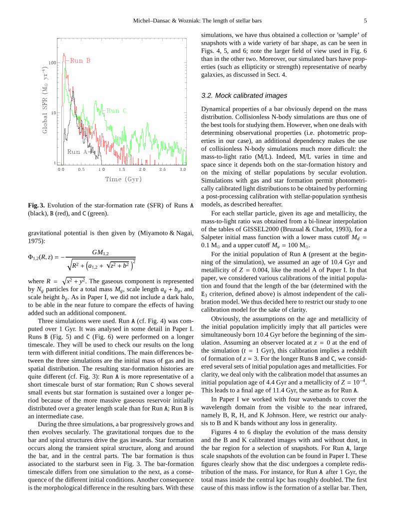
Fig. 3. Evolution of the star-formation rate (SFR) of RunsA(black),B (red), andC (green).

gravitational potential is then given by (Miyamoto & Nagai,1975):

Φ1,2(R, z) = −GM1,2

√

R2 +(

a1,2 +√

z2 + b2)2

whereR =√

x2 + y2. The gaseous component is representedby Ng particles for a total massMg, scale lengthag + bg, andscale heightbg. As in Paper I, we did not include a dark halo,to be able in the near future to compare the effects of havingadded such an additional component.

Three simulations were used. RunA (cf. Fig. 4) was com-puted over 1 Gyr. It was analysed in some detail in Paper I.RunsB (Fig. 5) andC (Fig. 6) were performed on a longertimescale. They will be used to check our results on the longterm with different initial conditions. The main differences be-tween the three simulations are the initial mass of gas and itsspatial distribution. The resulting star-formation histories arequite different (cf. Fig. 3): RunA is more representative of ashort timescale burst of star formation; RunC shows severalsmall events but star formation is sustained over a longer pe-riod because of the more massive gaseous reservoir initiallydistributed over a greater length scale than for RunA; RunB isan intermediate case.

During the three simulations, a bar progressively grows andthen evolves secularly. The gravitational torques due to thebar and spiral structures drive the gas inwards. Star formationoccurs along the transient spiral structure, along and aroundthe bar, and in the central parts. The bar formation is thusassociated to the starburst seen in Fig. 3. The bar-formationtimescale differs from one simulation to the next, as a conse-quence of the different initial conditions. Another consequenceis the morphological difference in the resulting bars. With these

simulations, we have thus obtained a collection or ’sample’ofsnapshots with a wide variety of bar shape, as can be seen inFigs. 4, 5, and 6; note the larger field of view used in Fig. 6than in the other two. Moreover, our simulated bars have prop-erties (such as ellipticity or strength) representative ofnearbygalaxies, as discussed in Sect. 4.

3.2. Mock calibrated images

Dynamical properties of a bar obviously depend on the massdistribution. Collisionless N-body simulations are thus one ofthe best tools for studying them. However, when one deals withdetermining observational properties (i.e. photometric prop-erties in our case), an additional dependency makes the useof collisionless N-body simulations much more difficult: themass-to-light ratio (M/L). Indeed, M/L varies in time andspace since it depends both on the star-formation history andon the mixing of stellar populations by secular evolution.Simulations with gas and star formation permit photometri-cally calibrated light distributions to be obtained by performinga post-processing calibration with stellar-population synthesismodels, as described hereafter.

For each stellar particle, given its age and metallicity, themass-to-light ratio was obtained from a bi-linear interpolationof the tables of GISSEL2000 (Bruzual & Charlot, 1993), for aSalpeter initial mass function with a lower mass cutoff Md =

0.1 M⊙ and a upper cutoff Mu = 100 M⊙.For the initial population of RunA (present at the begin-

ning of the simulation), we assumed an age of 10.4 Gyr andmetallicity of Z = 0.004, like the model A of Paper I. In thatpaper, we considered various calibrations of the initial popula-tion and found that the length of the bar (determined with theE3 criterion, defined above) is almost independent of the cali-bration model. We thus decided here to restrict our study to onecalibration model for the sake of clarity.

Obviously, the assumptions on the age and metallicity ofthe initial population implicitly imply that all particlesweresimultaneously born 10.4 Gyr before the beginning of the sim-ulation. Assuming an observer located atz = 0 at the end ofthe simulation (t = 1 Gyr), this calibration implies a redshiftof formation ofz = 3. For the longer RunsB andC, we consid-ered several sets of initial population ages and metallicities. Forclarity, we deal only with the calibration model that assumes aninitial population age of 4.4 Gyr and a metallicity ofZ = 10−4.This leads to a final age of 11.4 Gyr, the same as for RunA.

In Paper I we worked with four wavebands to cover thewavelength domain from the visible to the near infrared,namely B, R, H, and K Johnson. Here, we restrict our analy-sis to B and K bands without any loss in generality.

Figures 4 to 6 display the evolution of the mass densityand the B and K calibrated images with and without dust, inthe bar region for a selection of snapshots. For RunA, largescale snapshots of the evolution can be found in Paper I. Thesefigures clearly show that the disc undergoes a complete redis-tribution of the mass. For instance, for RunA after 1 Gyr, thetotal mass inside the central kpc has roughly doubled. The firstcause of this mass inflow is the formation of a stellar bar. Then,


Table 1. Initial parameters of the simulations

Run Ns Ng M1 M2 Mg a1 a2 b ag bg

A 500 000 50 000 1010 1011 1.1 1010 0.5 3.0 0.5 3.0 10−4

B 500 000 10 000 1010 1011 3.66 1010 0.5 3.0 0.5 3.0 0.5C 600 000 10 000 2 1010 1011 4 1010 0.5 5.0 1.0 10.0 0.5

Fig. 4. Evolution of RunA from t = 0 to t = 1 Gyr. From left to right are displayed the mass distribution(in log of M⊙ pc−2)and the calibrated images (B dust-free, B with extinction, Kdust-free, and K with extinction) in mag arcsec−2. The field of view(10 kpc) is the same for each frame. The particles have been rotated so that the bar position is roughly horizontal. Greyscaleimages and isocontours of mass surface density range from 101 to 105.2 M⊙ pc−2. Mass isocontours are logarithmically spacedby 0.47 log(M⊙ pc−2). The B greyscale images range from 11 to 26 mag arcsec−2, while contours range from 20 to 23 magarcsec−2 and are spaced by 1 mag. The K images range from 9 to 22 mag arcsec−2; K isocontours range from 17 to 20 magarcsec−2 and are spaced by 1 mag.


Fig. 5. Like Fig. 4 but for RunB from t = 0 to t = 5 Gyr. Greyscale images and isocontours of mass surface density range from101 to 105.2 M⊙ pc−2. Mass isocontours are logarithmically spaced by 0.47 log(M⊙ pc−2). The B greyscale images range from12 to 27 mag arcsec−2, while contours range from 19 to 23 mag arcsec−2 and are spaced by 1 mag. The K images range from 10to 23 mag arcsec−2; K isocontours range from 16 to 20 mag arcsec−2 and are spaced by 1 mag.

Fig. 6. Like Fig. 4 but for RunC from t = 0 to t = 5 Gyr. The field of view is 16 kpc. Greyscale images and isocontours ofmass surface density range from 101 to 105 M⊙ pc−2. Mass isocontours are logarithmically spaced by 0.44 log(M⊙ pc−2). The Bgreyscale images range from 13 to 27 mag arcsec−2, while contours range from 19 to 23 mag arcsec−2 and are spaced by 1 mag.The K images range from 10 to 23 mag arcsec−2; K isocontours range from 16 to 20 mag arcsec−2 and are spaced by 1 mag.

due to the gravitational torques exerted on the gas by the stellarbar, the extra mass in the form of gas and new stars amountsto 3.5 109 M⊙ at t = 1 Gyr for RunA, which is only 30% ofthe whole additional mass. In fact, the initial stellar populationcontributes to the other 70%.

After individual particle photometric calibration, mockCCD images were obtained summing particle luminosities intoa 512×512 pixels grid. The field of view was 60 kpc, whichgave a spatial resolution of≈ 117 pc, 1.3 times our small-est N-body grid resolution. We thus produced one frame perwaveband and per snapshot of the simulation. Our results areobviously independent of the bar PA with respect to the Northor any other axis. We thus decided to systematically rotate thepositions of particles to align the bar with the x-axis.

To mimic real observations we should have to convolve ourimages with a point-spread function. However, this last stagedepends on the telescope and observation-site characteristics.It thus introduces a few free parameters that cannot be con-strained without any detailed comparisons with real observa-tions, which is not our purpose.

3.3. Dust extinction

Dust extinction in B and K bands was simulated assuming aconstant gas-to-dust ratio

N(H i)/AV = 5.34× 1021cm−2.

Then,AV is converted toAB andAK . Extinction was computedin a cube with the same spatial resolution as for our imagesand 11 slabs along the line-of-sight (cf. Paper I for more de-tails). Each slab absorbs the stellar luminosity behind it.Foreach slab, the gas density distribution is obtained by convolv-ing particle positions with the SPH kernel.

4. Tests of bar-radii criteria on numericalsimulations

Each mock image was analysed by fitting simple ellipses tothe isophotes. Profiles of surface brightness, ellipticities, andPA were obtained by increasing the half-major axis lengthaby a factor 1.01 between each fit. We chose such a low valueto obtain a good resolution in the inner region. We display theresults for RunA in Figs. 7 and 8 for the same selected times asin Fig. 4. Results for the other runs are qualitatively similar, sothey are not displayed.

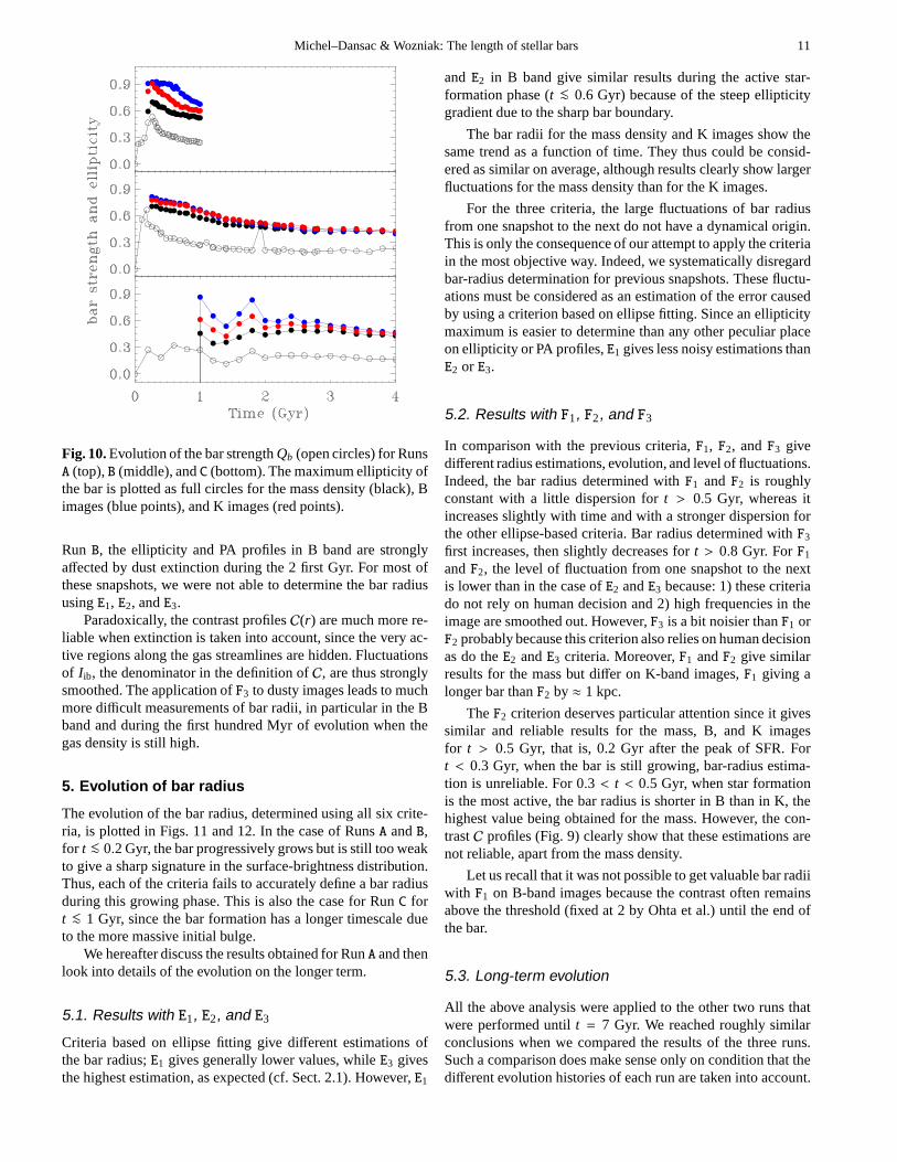
The ellipticity profiles in both bands are significantly dif-ferent fort < 1 Gyr. In Paper I, we proposed that, even in theabsence of extinction, two causes are simultaneously responsi-ble for the wavelength dependence of ellipticity profiles. First,the spatial distribution of the new population is very elongatedalong the bar because of new stars born in the gas flow alongthe bar that is narrower than the stellar bar. Then, secular evo-lution is responsible for progressively making it rounder.Thisexplains the high ellipticity reached in the bar when the star-formation rate (SFR) is high (t < 0.5 Gyr for RunA) and,only in part, the subsequent decrease. Second, the luminosityratio between the new and the initial populations is wavelengthdependent, being higher in B than in K band. After the SFRmaximum, the morphology becomes gradually dominated bythe luminosity of the initial population that has a rounder spa-tial distribution. When dust extinction is taken into account,especially in the B band, there is no longer a uniqueemax be-cause the real maximum is located in the dustiest region (e.g.t = 0.3 Gyr in Fig. 8). A comparison between B and K-bandE1 measurements confirms that ellipticity is strongly dependenton the colour.

It is interesting to compare the maximum ellipticity withthe bar strengthQb defined as (Combes & Sanders, 1981):

Qb = max

(

Fmaxθ

(r)

< FR(r) >

)

whereFmaxθ

(r) is the maximum tangential force at radiusr and< FR(r) > is the average radial force from the axisymmetriccomponent. Recently, this bar strength estimator has been alsoused in photometric studies (Buta & Block 2001, Buta et al.2005). Comparison of the evolution of the bar ellipticity withthat of Qb (cf. Fig. 10) clearly confirms that the bar axis ra-tio (or ellipticity) is not an estimator of the bar strengthQb.Indeed, bars with larger quadrupole moments and lower axisratios can have the sameQb as bars with smaller quadrupolemoments and higher axis ratios. Moreover, the radius at whichQ(r) reaches its maximum, used to defineQb, is always locatedin the circumnuclear region. Thus,Q(r) or Qb is not useful fordetermining the bar radius. The distributions ofQb for our sim-ulations and for real galaxies (Buta et al., 2005) are very sim-ilar, except forQb < 0.15 (very weak bars). Bar morphologyand properties, such as strength and ellipticity, producedin oursimulations are thus representative of real galaxies in thelocaluniverse.

Due to the definition ofE2 andE3, PA variations are<∼ 10

within the radial range defined byE2 andE3 criteria. This region


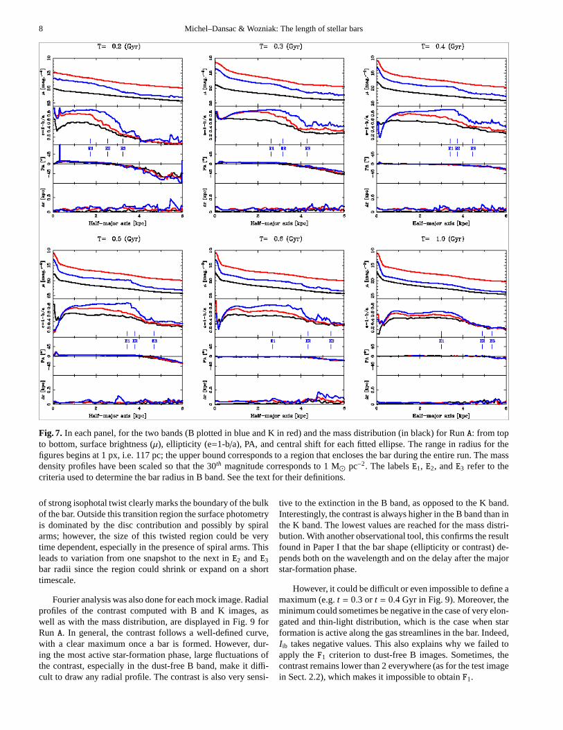
Fig. 7. In each panel, for the two bands (B plotted in blue and K in red)and the mass distribution (in black) for RunA: from topto bottom, surface brightness (µ), ellipticity (e=1-b/a), PA, and central shift for each fitted ellipse. The range inradius for thefigures begins at 1 px, i.e. 117 pc; the upper bound corresponds to a region that encloses the bar during the entire run. The massdensity profiles have been scaled so that the 30th magnitude corresponds to 1 M⊙ pc−2. The labelsE1, E2, andE3 refer to thecriteria used to determine the bar radius in B band. See the text for their definitions.

of strong isophotal twist clearly marks the boundary of the bulkof the bar. Outside this transition region the surface photometryis dominated by the disc contribution and possibly by spiralarms; however, the size of this twisted region could be verytime dependent, especially in the presence of spiral arms. Thisleads to variation from one snapshot to the next inE2 andE3

bar radii since the region could shrink or expand on a shorttimescale.

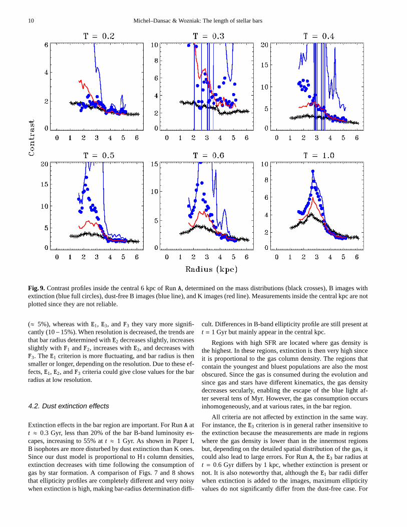
Fourier analysis was also done for each mock image. Radialprofiles of the contrast computed with B and K images, aswell as with the mass distribution, are displayed in Fig. 9 forRun A. In general, the contrast follows a well-defined curve,with a clear maximum once a bar is formed. However, dur-ing the most active star-formation phase, large fluctuations ofthe contrast, especially in the dust-free B band, make it diffi-cult to draw any radial profile. The contrast is also very sensi-

tive to the extinction in the B band, as opposed to the K band.Interestingly, the contrast is always higher in the B band than inthe K band. The lowest values are reached for the mass distri-bution. With another observational tool, this confirms the resultfound in Paper I that the bar shape (ellipticity or contrast)de-pends both on the wavelength and on the delay after the majorstar-formation phase.

However, it could be difficult or even impossible to define amaximum (e.g.t = 0.3 or t = 0.4 Gyr in Fig. 9). Moreover, theminimum could sometimes be negative in the case of very elon-gated and thin-light distribution, which is the case when starformation is active along the gas streamlines in the bar. Indeed,Iib takes negative values. This also explains why we failed toapply theF1 criterion to dust-free B images. Sometimes, thecontrast remains lower than 2 everywhere (as for the test imagein Sect. 2.2), which makes it impossible to obtainF1.


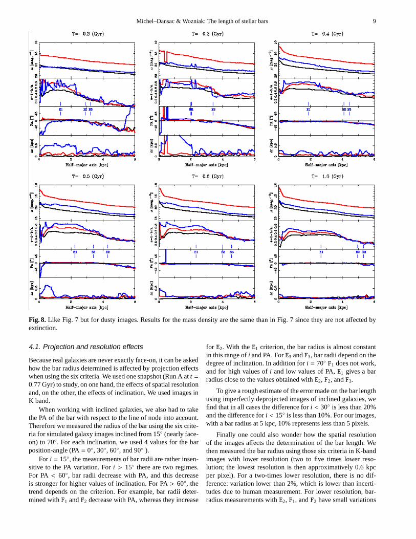
Fig. 8. Like Fig. 7 but for dusty images. Results for the mass densityare the same than in Fig. 7 since they are not affected byextinction.

4.1. Projection and resolution effects

Because real galaxies are never exactly face-on, it can be askedhow the bar radius determined is affected by projection effectswhen using the six criteria. We used one snapshot (Run A att =0.77 Gyr) to study, on one hand, the effects of spatial resolutionand, on the other, the effects of inclination. We used images inK band.

When working with inclined galaxies, we also had to takethe PA of the bar with respect to the line of node into account.Therefore we measured the radius of the bar using the six crite-ria for simulated galaxy images inclined from 15 (nearly face-on) to 70. For each inclination, we used 4 values for the barposition-angle (PA= 0, 30, 60, and 90 ).

For i = 15, the measurements of bar radii are rather insen-sitive to the PA variation. Fori > 15 there are two regimes.For PA < 60, bar radii decrease with PA, and this decreaseis stronger for higher values of inclination. For PA> 60, thetrend depends on the criterion. For example, bar radii deter-mined withF1 andF2 decrease with PA, whereas they increase

for E2. With theE1 criterion, the bar radius is almost constantin this range ofi and PA. ForE3 andF3, bar radii depend on thedegree of inclination. In addition fori = 70 F1 does not work,and for high values ofi and low values of PA,E1 gives a barradius close to the values obtained withE2, F2, andF3.

To give a rough estimate of the error made on the bar lengthusing imperfectly deprojected images of inclined galaxies, wefind that in all cases the difference fori < 30 is less than 20%and the difference fori < 15 is less than 10%. For our images,with a bar radius at 5 kpc, 10% represents less than 5 pixels.

Finally one could also wonder how the spatial resolutionof the images affects the determination of the bar length. Wethen measured the bar radius using those six criteria in K-bandimages with lower resolution (two to five times lower reso-lution; the lowest resolution is then approximatively 0.6 kpcper pixel). For a two-times lower resolution, there is no dif-ference: variation lower than 2%, which is lower than incerti-tudes due to human measurement. For lower resolution, bar-radius measurements withE2, F1, andF2 have small variations


Fig. 9. Contrast profiles inside the central 6 kpc of RunA, determined on the mass distributions (black crosses), B images withextinction (blue full circles), dust-free B images (blue line), and K images (red line). Measurements inside the central kpc are notplotted since they are not reliable.

(≈ 5%), whereas withE1, E3, andF3 they vary more signifi-cantly (10−15%). When resolution is decreased, the trends arethat bar radius determined withE2 decreases slightly, increasesslightly with F1 andF2, increases withE3, and decreases withF3. TheE1 criterion is more fluctuating, and bar radius is thensmaller or longer, depending on the resolution. Due to theseef-fects,E1, E2, andF3 criteria could give close values for the barradius at low resolution.

4.2. Dust extinction effects

Extinction effects in the bar region are important. For RunA att ≈ 0.3 Gyr, less than 20% of the bar B-band luminosity es-capes, increasing to 55% att ≈ 1 Gyr. As shown in Paper I,B isophotes are more disturbed by dust extinction than K ones.Since our dust model is proportional to H column densities,extinction decreases with time following the consumption ofgas by star formation. A comparison of Figs. 7 and 8 showsthat ellipticity profiles are completely different and very noisywhen extinction is high, making bar-radius determination diffi-

cult. Differences in B-band ellipticity profile are still present att = 1 Gyr but mainly appear in the central kpc.

Regions with high SFR are located where gas density isthe highest. In these regions, extinction is then very high sinceit is proportional to the gas column density. The regions thatcontain the youngest and bluest populations are also the mostobscured. Since the gas is consumed during the evolution andsince gas and stars have different kinematics, the gas densitydecreases secularly, enabling the escape of the blue light af-ter several tens of Myr. However, the gas consumption occursinhomogeneously, and at various rates, in the bar region.

All criteria are not affected by extinction in the same way.For instance, theE3 criterion is in general rather insensitive tothe extinction because the measurements are made in regionswhere the gas density is lower than in the innermost regionsbut, depending on the detailed spatial distribution of the gas, itcould also lead to large errors. For RunA, theE3 bar radius att = 0.6 Gyr differs by 1 kpc, whether extinction is present ornot. It is also noteworthy that, although theE1 bar radii differwhen extinction is added to the images, maximum ellipticityvalues do not significantly differ from the dust-free case. For


Fig. 10.Evolution of the bar strengthQb (open circles) for RunsA (top),B (middle), andC (bottom). The maximum ellipticity ofthe bar is plotted as full circles for the mass density (black), Bimages (blue points), and K images (red points).

Run B, the ellipticity and PA profiles in B band are stronglyaffected by dust extinction during the 2 first Gyr. For most ofthese snapshots, we were not able to determine the bar radiususingE1, E2, andE3.

Paradoxically, the contrast profilesC(r) are much more re-liable when extinction is taken into account, since the veryac-tive regions along the gas streamlines are hidden. Fluctuationsof Iib, the denominator in the definition ofC, are thus stronglysmoothed. The application ofF3 to dusty images leads to muchmore difficult measurements of bar radii, in particular in the Bband and during the first hundred Myr of evolution when thegas density is still high.

5. Evolution of bar radius

The evolution of the bar radius, determined using all six crite-ria, is plotted in Figs. 11 and 12. In the case of RunsA andB,for t <∼ 0.2 Gyr, the bar progressively grows but is still too weakto give a sharp signature in the surface-brightness distribution.Thus, each of the criteria fails to accurately define a bar radiusduring this growing phase. This is also the case for RunC fort <∼ 1 Gyr, since the bar formation has a longer timescale dueto the more massive initial bulge.

We hereafter discuss the results obtained for RunA and thenlook into details of the evolution on the longer term.

5.1. Results with E1, E2, and E3

Criteria based on ellipse fitting give different estimations ofthe bar radius;E1 gives generally lower values, whileE3 givesthe highest estimation, as expected (cf. Sect. 2.1). However, E1

andE2 in B band give similar results during the active star-formation phase (t <∼ 0.6 Gyr) because of the steep ellipticitygradient due to the sharp bar boundary.

The bar radii for the mass density and K images show thesame trend as a function of time. They thus could be consid-ered as similar on average, although results clearly show largerfluctuations for the mass density than for the K images.

For the three criteria, the large fluctuations of bar radiusfrom one snapshot to the next do not have a dynamical origin.This is only the consequence of our attempt to apply the criteriain the most objective way. Indeed, we systematically disregardbar-radius determination for previous snapshots. These fluctu-ations must be considered as an estimation of the error causedby using a criterion based on ellipse fitting. Since an ellipticitymaximum is easier to determine than any other peculiar placeon ellipticity or PA profiles,E1 gives less noisy estimations thanE2 or E3.

5.2. Results with F1, F2, and F3

In comparison with the previous criteria,F1, F2, andF3 givedifferent radius estimations, evolution, and level of fluctuations.Indeed, the bar radius determined withF1 andF2 is roughlyconstant with a little dispersion fort > 0.5 Gyr, whereas itincreases slightly with time and with a stronger dispersionforthe other ellipse-based criteria. Bar radius determined with F3

first increases, then slightly decreases fort > 0.8 Gyr. ForF1

andF2, the level of fluctuation from one snapshot to the nextis lower than in the case ofE2 andE3 because: 1) these criteriado not rely on human decision and 2) high frequencies in theimage are smoothed out. However,F3 is a bit noisier thanF1 orF2 probably because this criterion also relies on human decisionas do theE2 andE3 criteria. Moreover,F1 andF2 give similarresults for the mass but differ on K-band images,F1 giving alonger bar thanF2 by≈ 1 kpc.

TheF2 criterion deserves particular attention since it givessimilar and reliable results for the mass, B, and K imagesfor t > 0.5 Gyr, that is, 0.2 Gyr after the peak of SFR. Fort < 0.3 Gyr, when the bar is still growing, bar-radius estima-tion is unreliable. For 0.3 < t < 0.5 Gyr, when star formationis the most active, the bar radius is shorter in B than in K, thehighest value being obtained for the mass. However, the con-trastC profiles (Fig. 9) clearly show that these estimations arenot reliable, apart from the mass density.

Let us recall that it was not possible to get valuable bar radiiwith F1 on B-band images because the contrast often remainsabove the threshold (fixed at 2 by Ohta et al.) until the end ofthe bar.

5.3. Long-term evolution

All the above analysis were applied to the other two runs thatwere performed untilt = 7 Gyr. We reached roughly similarconclusions when we compared the results of the three runs.Such a comparison does make sense only on condition that thedifferent evolution histories of each run are taken into account.


Fig. 11.Bar and resonance radii for RunsA, B, andC. For each panel, lines represent the ILR (shorter radius), UHR (intermediateradius), and CR (greater radius). The dimmed region shows theL1,2–L4,5 range. Bar radii determined with the maximum ellipticitycriterion (E1) are plotted as open triangles, those determined with the minimum ellipticity criterion (E3) are plotted with opensquares, and the new criterion (E2) is represented by full circles.Top panels:bar radii determined for the mass.Middle panels:B dust-free images.Bottom panels:K dust-free images.

The first Gyr of RunA is therefore comparable to almost thefirst 1.5 Gyr of RunB and the first 3 Gyr of RunC.

The differences between RunA and the two other runsmainly concern the criteriaE1 andF1 to F3. For RunB, theF1

criterion can be measured from B-band images, and the resultsare similar to those in K band. For RunC, the measurements us-ing this criterion are possible and reliable fort >∼ 2 Gyr and givethe same values as theF2 criterion. Another difference concerns

theE1 criterion for RunC. Indeed, it gives approximatively thesame values as theE2 criterion for t <∼ 3 Gyr. TheF3 criteriongives a significantly greater bar radius than those obtainedwithF1 andF2. This criterion is very comparable toE2.

On the other hand, for the criteriaE2, E3, andF1 to F3, eachgives similar results when we determine bar radius on the B orK-band images or on mass distributions, taking the uncertain-ties of measurements into account.


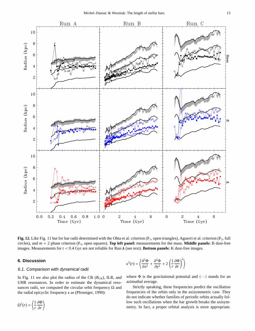
Fig. 12.Like Fig. 11 but for bar radii determined with the Ohta et al. criterion (F1, open triangles), Aguerri et al. criterion (F2, fullcircles), andm = 2 phase criterion (F3, open squares).Top left panel: measurements for the mass.Middle panels: B dust-freeimages. Measurements fort < 0.4 Gyr are not reliable for RunA (see text).Bottom panels:K dust-free images.

6. Discussion

6.1. Comparison with dynamical radii

In Fig. 11 we also plot the radius of the CR (RCR), ILR, andUHR resonances. In order to estimate the dynamical reso-nances radii, we computed the circular orbit frequencyΩ andthe radial epicyclic frequencyκ as (Pfenniger, 1990):

Ω2(r) =

⟨

1r∂Φ

∂r

⟩

κ2(r) =

⟨

∂2Φ

∂x2+∂2Φ

∂y2+ 2

(

1r∂Φ

∂r

)2⟩

whereΦ is the gravitational potential and〈· · ·〉 stands for anazimuthal average.

Strictly speaking, these frequencies predict the oscillationfrequencies of the orbits only in the axisymmetric case. Theydo not indicate whether families of periodic orbits actually fol-low such oscillations when the bar growth breaks the axisym-metry. In fact, a proper orbital analysis is more appropriate.


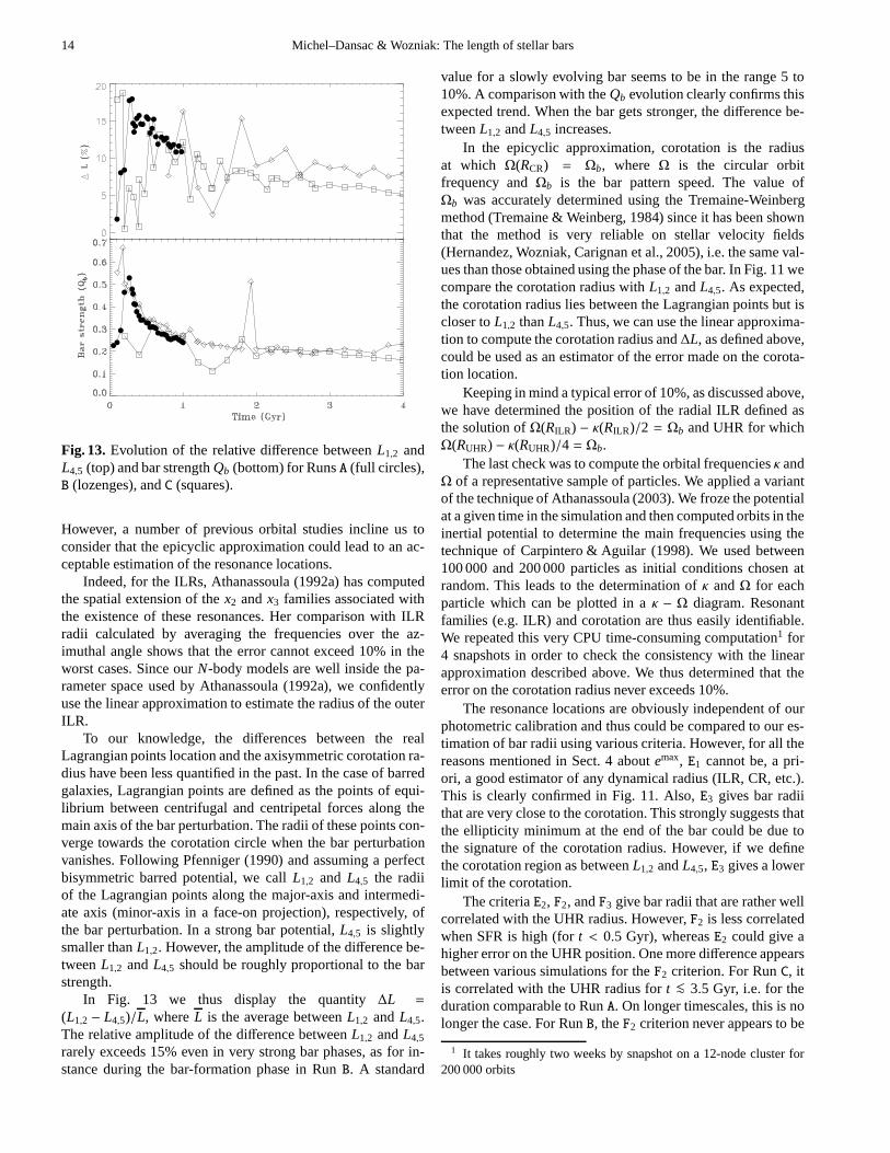
Fig. 13. Evolution of the relative difference betweenL1,2 andL4,5 (top) and bar strengthQb (bottom) for RunsA (full circles),B (lozenges), andC (squares).

However, a number of previous orbital studies incline us toconsider that the epicyclic approximation could lead to an ac-ceptable estimation of the resonance locations.

Indeed, for the ILRs, Athanassoula (1992a) has computedthe spatial extension of thex2 andx3 families associated withthe existence of these resonances. Her comparison with ILRradii calculated by averaging the frequencies over the az-imuthal angle shows that the error cannot exceed 10% in theworst cases. Since ourN-body models are well inside the pa-rameter space used by Athanassoula (1992a), we confidentlyuse the linear approximation to estimate the radius of the outerILR.

To our knowledge, the differences between the realLagrangian points location and the axisymmetric corotation ra-dius have been less quantified in the past. In the case of barredgalaxies, Lagrangian points are defined as the points of equi-librium between centrifugal and centripetal forces along themain axis of the bar perturbation. The radii of these points con-verge towards the corotation circle when the bar perturbationvanishes. Following Pfenniger (1990) and assuming a perfectbisymmetric barred potential, we callL1,2 and L4,5 the radiiof the Lagrangian points along the major-axis and intermedi-ate axis (minor-axis in a face-on projection), respectively, ofthe bar perturbation. In a strong bar potential,L4,5 is slightlysmaller thanL1,2. However, the amplitude of the difference be-tweenL1,2 andL4,5 should be roughly proportional to the barstrength.

In Fig. 13 we thus display the quantity∆L =

(L1,2 − L4,5)/L, whereL is the average betweenL1,2 andL4,5.The relative amplitude of the difference betweenL1,2 andL4,5

rarely exceeds 15% even in very strong bar phases, as for in-stance during the bar-formation phase in RunB. A standard

value for a slowly evolving bar seems to be in the range 5 to10%. A comparison with theQb evolution clearly confirms thisexpected trend. When the bar gets stronger, the difference be-tweenL1,2 andL4,5 increases.

In the epicyclic approximation, corotation is the radiusat which Ω(RCR) = Ωb, where Ω is the circular orbitfrequency andΩb is the bar pattern speed. The value ofΩb was accurately determined using the Tremaine-Weinbergmethod (Tremaine & Weinberg, 1984) since it has been shownthat the method is very reliable on stellar velocity fields(Hernandez, Wozniak, Carignan et al., 2005), i.e. the same val-ues than those obtained using the phase of the bar. In Fig. 11 wecompare the corotation radius withL1,2 andL4,5. As expected,the corotation radius lies between the Lagrangian points but iscloser toL1,2 thanL4,5. Thus, we can use the linear approxima-tion to compute the corotation radius and∆L, as defined above,could be used as an estimator of the error made on the corota-tion location.

Keeping in mind a typical error of 10%, as discussed above,we have determined the position of the radial ILR defined asthe solution ofΩ(RILR) − κ(RILR)/2 = Ωb and UHR for whichΩ(RUHR) − κ(RUHR)/4 = Ωb.

The last check was to compute the orbital frequenciesκ andΩ of a representative sample of particles. We applied a variantof the technique of Athanassoula (2003). We froze the potentialat a given time in the simulation and then computed orbits in theinertial potential to determine the main frequencies usingthetechnique of Carpintero & Aguilar (1998). We used between100 000 and 200 000 particles as initial conditions chosen atrandom. This leads to the determination ofκ andΩ for eachparticle which can be plotted in aκ − Ω diagram. Resonantfamilies (e.g. ILR) and corotation are thus easily identifiable.We repeated this very CPU time-consuming computation1 for4 snapshots in order to check the consistency with the linearapproximation described above. We thus determined that theerror on the corotation radius never exceeds 10%.

The resonance locations are obviously independent of ourphotometric calibration and thus could be compared to our es-timation of bar radii using various criteria. However, for all thereasons mentioned in Sect. 4 aboutemax, E1 cannot be, a pri-ori, a good estimator of any dynamical radius (ILR, CR, etc.).This is clearly confirmed in Fig. 11. Also,E3 gives bar radiithat are very close to the corotation. This strongly suggests thatthe ellipticity minimum at the end of the bar could be due tothe signature of the corotation radius. However, if we definethe corotation region as betweenL1,2 andL4,5, E3 gives a lowerlimit of the corotation.

The criteriaE2, F2, andF3 give bar radii that are rather wellcorrelated with the UHR radius. However,F2 is less correlatedwhen SFR is high (fort < 0.5 Gyr), whereasE2 could give ahigher error on the UHR position. One more difference appearsbetween various simulations for theF2 criterion. For RunC, itis correlated with the UHR radius fort <∼ 3.5 Gyr, i.e. for theduration comparable to RunA. On longer timescales, this is nolonger the case. For RunB, theF2 criterion never appears to be

1 It takes roughly two weeks by snapshot on a 12-node cluster for200 000 orbits


correlated with the UHR radius, and it gives values between theILR and the UHR radius. Nevertheless,E2 andF3 criteria arestill correlated with the UHR radius on longer timescales, liketheE3 criterion with the corotation radius.

The fact thatE2, F3, and in some casesF2 criteria aregood estimators of the UHR radius during the first Gyr canbe understood in the framework of stellar orbits. Indeed, ithas been shown (Contopoulos, 1981a) that the UHR (or 4/1resonance) is a gap where no family of periodic orbits canexist. Moreover, between the UHR and the corotation, mostfamilies of periodic orbits are unstable (Contopoulos, 1981b)if the bar perturbation is stronger than 10% of the potentialbackground (the stellar disc). Using 3D models, Skokos et al.(2002) also conclude that the most appropriate orbits to sustaina bar are those inside the UHR. Thus, between the UHR andthe corotation, a bar is mostly sustained by semi-chaotic orbits(Wozniak & Pfenniger, 1999). The density response of thesesemi-chaotic orbits in the configuration space is rounder thanthe response density of orbits trapped around the major fam-ilies of periodic orbits (i.e.x1 and 3/1 resonant family). Thusthe contrast as defined by Eq. (1) should strongly decrease af-ter the UHR. This also explains whyE3 is a good tracer of thecorotation radius.

However, for RunC, theF2 criterion is no longer correlatedwith the UHR radius fromt >∼ 3.5 Gyr and never appears tobe correlated with the UHR radius for RunB. This means thatthis criterion is not a reliable estimator of the resonance loca-tion. The bar–interbar contrast indeed shows the pattern ofthebar for all the snapshots of these three runs, but the decreaseof the contrast at the end of the bar, which is the transition re-gion between the bar and the disc, seems to be very sensitiveto local conditions (such as star formation at the end of the bar,the spiral structure in the disc, and the thickness of the disc);therefore, these measurements depend on the type of bar andevolution. Then, even if theF2 criterion is an automatic and re-liable criterion of the bar radius, it defines a radius that isnotalways correlated with a resonance and then is not comparablefrom one to another galaxy.

6.2. Fast and slow bars

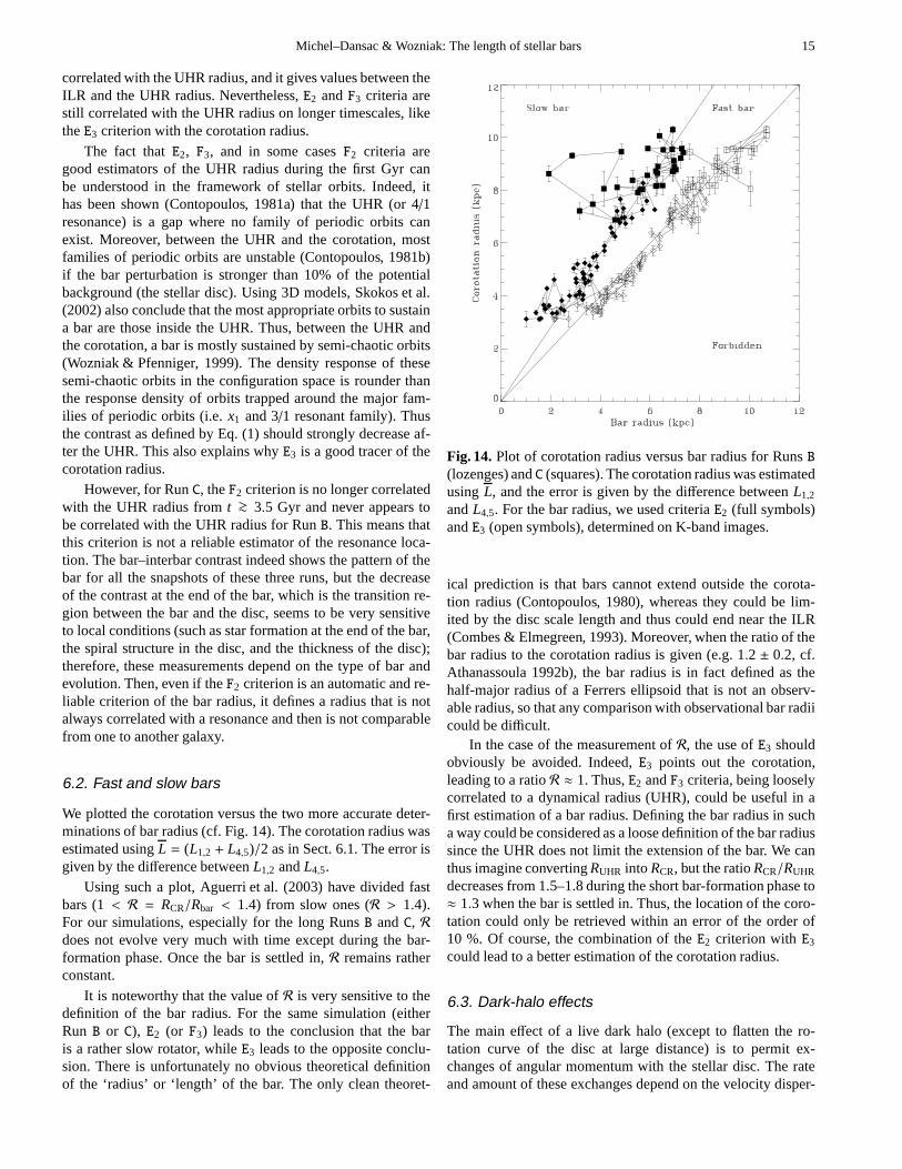
We plotted the corotation versus the two more accurate deter-minations of bar radius (cf. Fig. 14). The corotation radiuswasestimated usingL = (L1,2 + L4,5)/2 as in Sect. 6.1. The error isgiven by the difference betweenL1,2 andL4,5.

Using such a plot, Aguerri et al. (2003) have divided fastbars (1< R = RCR/Rbar < 1.4) from slow ones (R > 1.4).For our simulations, especially for the long RunsB andC, Rdoes not evolve very much with time except during the bar-formation phase. Once the bar is settled in,R remains ratherconstant.

It is noteworthy that the value ofR is very sensitive to thedefinition of the bar radius. For the same simulation (eitherRun B or C), E2 (or F3) leads to the conclusion that the baris a rather slow rotator, whileE3 leads to the opposite conclu-sion. There is unfortunately no obvious theoretical definitionof the ‘radius’ or ‘length’ of the bar. The only clean theoret-

Fig. 14.Plot of corotation radius versus bar radius for RunsB(lozenges) andC (squares). The corotation radius was estimatedusingL, and the error is given by the difference betweenL1,2

andL4,5. For the bar radius, we used criteriaE2 (full symbols)andE3 (open symbols), determined on K-band images.

ical prediction is that bars cannot extend outside the corota-tion radius (Contopoulos, 1980), whereas they could be lim-ited by the disc scale length and thus could end near the ILR(Combes & Elmegreen, 1993). Moreover, when the ratio of thebar radius to the corotation radius is given (e.g. 1.2 ± 0.2, cf.Athanassoula 1992b), the bar radius is in fact defined as thehalf-major radius of a Ferrers ellipsoid that is not an observ-able radius, so that any comparison with observational bar radiicould be difficult.

In the case of the measurement ofR, the use ofE3 shouldobviously be avoided. Indeed,E3 points out the corotation,leading to a ratioR ≈ 1. Thus,E2 andF3 criteria, being looselycorrelated to a dynamical radius (UHR), could be useful in afirst estimation of a bar radius. Defining the bar radius in sucha way could be considered as a loose definition of the bar radiussince the UHR does not limit the extension of the bar. We canthus imagine convertingRUHR into RCR, but the ratioRCR/RUHR

decreases from 1.5–1.8 during the short bar-formation phase to≈ 1.3 when the bar is settled in. Thus, the location of the coro-tation could only be retrieved within an error of the order of10 %. Of course, the combination of theE2 criterion with E3

could lead to a better estimation of the corotation radius.

6.3. Dark-halo effects

The main effect of a live dark halo (except to flatten the ro-tation curve of the disc at large distance) is to permit ex-changes of angular momentum with the stellar disc. The rateand amount of these exchanges depend on the velocity disper-


sion of both the disc and the halo, and on the relative halomass (cf. Debattista & Sellwood 2000, Athanassoula 2003,Valenzuela & Klypin 2003). The stellar disc could lose be-tween a few % and 40% of its angular momentum. Dependingon the rate at which the stellar disc loses its angular momen-tum, the bar grows quite differently. The lack of dark halo in oursimulations thus has mainly three consequences on our work:

1) The evolution timescale could be different from simula-tions with a dark halo, leading us not to draw any conclusionabout the evolution ofR, for instance.

2) The shape and strength of a bar are also affectedby the presence of the live halo (Athanassoula & Misiriotis,2002). The central concentration of the halo is thus a key pa-rameter. For instance, Athanassoula & Misiriotis (2002) stressthat more centrally concentrated halos lead to rectangular-likebars. However, the photometric and morphological properties(shape, ellipticity,Qb, etc.; cf. also Paper I) of our simulatedbars are very representative of real stellar bars. For instance,we are able to reproduce a rectangular-like bar (RunB, Fig. 6).

3) The main results that could be affected by the absenceof a dark halo in our simulations are those related to dynamicalproperties, i.e. the correlation of the position of resonances withbar-radii estimators (Sect. 6.1). This is a major concern sincethere is a debate on whether a dark halo increasesR or not,leading to significantly smaller bars compared to corotation.Debattista & Sellwood (2000) report high values ofR for anumber of their simulations. However, Debattista & Sellwood(2000) estimate bar radii using in part theF3 criterion that is, forour simulations, quite correlated to UHR. This criterion givesrather short bars, since it is mainly influenced by the part ofthebar sustained byx1 orbits. This might explain the highR valuesin part. For the simulations by O’Neill & Dubinski (2003) andValenzuela & Klypin (2003),R remains in the range 1.2−1.7.Valenzuela & Klypin (2003) mainly use a criterion based onsurface density (not tested in the present paper), which seemsto give similar results thanF3, whereas O’Neill & Dubinski(2003) use an average of three methods (includingE2 andF3).

Our results should thus be confirmed with simulations thatinclude a live dark halo. However, the presence of a dissipa-tive component that can also exchange angular momentum andmass with the collisionless components through gravitationalinteraction, star formation, and feedback processes must havesome influence on the global angular momentum exchanges.Therefore, realistic models should now include both dark mat-ter and a dissipative component. This will be published else-where.

7. Conclusions

We have used N-body simulations, including stars, gas, andstar formation, that were photometrically calibrated in B andK wavebands to compare the bar lengths determined by six ob-servational criteria (five commonly applied to observations orsimulations and a sixth introduced in this paper). These crite-ria are based on ellipse fitting (E1 to E3) and Fourier analysis(F1 to F3) of the surface brightness (or mass surface density).The bar-length estimates were also compared to the locationofresonances.

We have obtained the following main results for each crite-rion in turn:

– E1 (Wozniak & Pierce, 1991), the radius of the maximumellipticity, gives the shortest bar lengths. It clearly underes-timates the real bar radius. Moreover, it is not linked to anydynamical characteristics of a bar (e.g. resonance).

– E2 is measured at the end of the PA plateau. It can be usedto approximately locate the UHR.

– E3, the radius of the minimum of ellipticity (Wozniak et al.,1995), gives the greatest bar lengths. In general, it is lesssensitive to dust absorption than other criteria. This is theonly criterion, amongst the six criteria tested, that is corre-lated with the corotation.

– F1 (Ohta et al., 1990) is not always defined, since the bar–interbar brightness contrast (C) could remain under 2 evenfor strong bars.

– F2 (Aguerri et al., 2000), also based onC, is the least noisyestimator. However it gives contradictory results for oursimulations.

– F3, widely used to determine the bar length in N−bodysimulations (e.g. Debattista & Sellwood 2000), gives barlengths comparable toE2 results. LikeE2, it gives quite agood approximation of the UHR location.

In general, for projection anglesi between 15 and 70, thebar length is underestimated with respect to its face-on value,apart from usingE1. However, fori < 30, errors remain below20%. Measurements also depend on the resolution but errorsnever exceed 15% when resolution is downgraded by a factor 5.

We moreover confirm that ellipticity profiles of B and K-band images can be very different. They also differ from ellip-ticity profiles of the mass density. This leads to a clear depen-dence of the maximum ellipticity on the waveband. Howeverthe radius of the maximum determined byE1 is less affected.Within a typical error of 10%, bar lengths determined withother criteria are not colour dependent, in the absence of dust.The situation is different when dust absorption is taken into ac-count. Criteria giving the smallest bar-length estimate are muchmore affected than others. This is the case ofE1 in particular.

For each simulation, the maximum ellipticity decreaseswith time, as do the bar strengthsQb, but not at the same rate.The use of the maximum ellipticity to estimate the bar strengthcould thus lead to severe errors, especially in a comparisonofone galaxy to another.

Accurate determination of the bar length is crucial in sev-eral observational or theoretical analyses. For instance,the ratioR = RCR/Rbar could increase from 1 (fast bar) to 1.4 (slow bar)just by usingE2 or F3 instead ofE3. However, being correlatedto the corotation radius,E3 cannot be used to define the end of abar. UsingE2 or F3 to define the end of the bar has physical im-plications since these criteria point out the UHR. Indeed, insidethe UHR, the bar is mainly sustained byx1 or other familiesof orbits elongated along the bar major-axis. However, thereis clear evidence that what is commonly called a bar extendsa bit outside the UHR because the region between UHR andCR is populated by higher resonant families of orbits, as wellas semi-chaotic and chaotic orbits that contribute to the shape(sometime rectangular-like) of the bar. The definition of the bar


length (hence the criterion used) should thus depend on the ap-plication.

Acknowledgements. We are grateful to Luis Aguilar and an anony-mous referee for comments and suggestions that have helped tostrengthen the conclusions of this paper. We would also liketothank Luis Aguilar for providing his code to compute orbitalfre-quencies. Our computations were partly performed on the FujitsuNEC SX-5 hosted by IDRIS/CNRS and the CRAL 18-node clusterof PC funded by the INSU/CNRS (ATIP # 2JE014 and ProgrammeNational Galaxie). LMD acknowledges support from a grant from theUniversidad Nacional Autonoma de Mexico (UNAM) for part of thiswork.

References

Aguerri J.A.L., Munoz-Tunon C., Varela A.M., Prieto M.,2000, A&A 361, 841

Aguerri J.A.L., Debattista V.P., Corsini E.M., 2003, MNRAS338, 465

Athanassoula E., 1992a, MNRAS 259, 328Athanassoula E., 1992b, MNRAS 259, 345Athanassoula E., 2003, MNRAS 341, 1179Athanassoula E., Morin S., Wozniak H., et al., 1990, MNRAS

245, 130Athanassoula E., Misiriotis A., 2002, MNRAS 330, 35Bruzual G., Charlot S., 1993, ApJ 405, 538Buta R., Block D.L., 2001, ApJ 550, 243Buta R., Combes F., 1996, Fund. Cosmic Phys. 17, 95Buta R., Vasylyev S., Salo H., Laurikainen E., 2005, AJ 130,

506Carpintero D.D., Aguilar L.A., 1998, MNRAS 298, 1Chapelon S., Contini T., Davoust E., 1999, A&A 345, 81Combes F., Sanders R.H., 1981, A&A 96, 164Combes F., Elmegreen E.,E., 1993, A&A 271, 391Contopoulos G., 1980, A&A 81, 198Contopoulos G., 1981a, CMDA 24, 355Contopoulos G., 1981b, A&A 102, 265Debattista V.P., Sellwood J.A., 2000, ApJ 543, 704Erwin P. Sparke L.S., 2003, ApJS 146, 299Friedli D., Benz W., 1993, A&A 268, 65Friedli D., Benz W., 1995, A&A 301, 649Heller C., Shlosman I., Englmaier P., 2001, ApJ 553, 661Hernandez O., Wozniak H., Carignan C., Amram P., Chemin

L., Daigle O., 2005, ApJ in pressJogee S., Barazza F. B., Rix H.-W., et al., 2004, ApJ 615, L105Jungwiert B., Combes F., Axon D. J., 1997, A&AS, 125, 479Kent S.M., 1990, AJ 100, 377Knapen J.H., Perez-Ramırez D., Laine S., 2002, MNRAS 337,

808Kormendy J., Kennicutt R.C., 2004, ARA& A 42, 603Laine S., Shlosman I., Knapen J. H., Peletier, R. F., 2002, ApJ,

567, 97Maeder A., 1992, A&A 264, 105Martin P., 1995, AJ 109, 2428Martinet L., Friedli D., 1997, A&A 323, 363Michel–Dansac L., Wozniak H., 2004, A&A 421, 863 (Paper I)Miyamoto M., Nagai R., 1975, PASJ 27, 533Monaghan, J. J., 1992, ARA&A 30, 543

Ohta K., Hamabe M., Wakamatsu K., 1990, ApJ 357, 71O’Neill J.K., Dubinski J., 2003, MNRAS 346, 251Patsis P.A., Skokos C., Athanassoula E., 2002, MNRAS 337,

578Pfenniger D., 1990, A&A 230, 55Pfenniger D., Friedli D., 1991, A&A 252, 75Pfenniger D., Friedli D., 1993, A&A 270, 561Rautiainen P., Salo H., 1999, A&A 348, 737Regan M.W., Elmegreen D.M., 1997, AJ 114, 965Regan M.W., Teuben P.J., 2004, ApJ 600, 595Sanders R.H., Tubbs A.D., 1980, ApJ 235, 803Sellwood J.A., Wilkinson A., 1993, Rep. Prog. Phys. 56, 173Sparke L.S., Sellwood J.A., 1987, MNRAS 225, 653Skokos C., Patsis P.A., Athanassoula E., 2002, MNRAS 333,

861Tremaine S., & Weinberg M. D. 1984, ApJ 282, L5Valenzuela O., Klypin A., 2003, MNRAS 345, 406Wozniak H., Friedli D., Martinet L. et al., 1995, A&AS 111,

115Wozniak H., Pfenniger D., 1999, CDMA 73, 149Wozniak H., Pierce, M.J., 1991, A&AS 88, 325

This figure "barlength05.png" is available in "png" format from:

http://arxiv.org/ps/astro-ph/0503406v2


This figure "barlength06.png" is available in "png" format from:



the length of stellar bars in sb galaxies and n body ... · the length of stellar bars in sb...

Documents