The Light-front constituent quark model

and the electromagnetic properties

of the nucleon:

beyond the valence component ?

Giovanni Salme

(Istituto Nazionale di Fisica Nucleare, Roma, Italy)

Relativistic quark models for the pion form factor in SL and TL

Phys. Lett. B 581 (2004) 75; Phys. Rev. D 73, 074013 (2006)

J.P.B.C. de Melo, T. Frederico, E. Pace, G. S.

Relativistic quark models for nucleon form factors in SL and TL

Phys. Lett. B 671 (2009) 153,

J.P.B.C. de Melo, T. Frederico, E. Pace, S. Pisano, G.S.

Nucleon electromagnetic form factors in the timelike region

Prog, Part. Nucl. Phys. 68, 113-157 (2013),

Achim Denig and G.S.

Motivations and Outline

The non perturbative regime appears the most challenging, in view

of the still non fully understood confinement mechanism ⇒Mikhail Shifman in a 2010-talk in honor of Murray Gell-Mann’s

80th birthday emphasized: Although the underlying QCD

Lagrangian and asymptotic freedom, it implies at short distances,

are established beyond any doubt, the road from this starting point

to theoretical control over the large-distance hadronic world is long

and difficult (M. Shifman, arXiv:1007.0531)

Goal: developing a covariant framework, based on the

Bethe-Salpeter Amplitudes of hadrons, or equivalently on the

Light-Front wave functions (Fock expansion) that allows one to

include information on hadron dynamics, extracted from processes

involving em probes in both space- and time-like regions This

provides a new tool for paving the way from a purely

phenomenological microscopic description of the hadronic states to

the one with a more consistent dynamical content.

Our strategy was:

first modeling the quark-photon vertex and the quark-hadron

amplitude from an investigation of the pion EM form factor, within

a Mandelstam-inspired approach. Then, moving to the nucleon case,

producing true predictions for the timelike region (it contains a lot

of information on mesonic spectra to be extracted...).

2

N.B. the approach have been extended to both Generalized Parton

Distributions and transverse-momentum distributions (presently

applied to the pion case, PRD D 80 (2009) 05444021, and first

results for the nucleon)

Why ”beyond relativistic constituent quark models” ?

Our personal experience:the attempt to describe nucleon ff’s in a

relativistic constituent quark model, within a Poincare’ covariant

Light-front approach, using only the nucleon valence vertex

function, compelled us to introduce CQ form factors..... Expected

from the quasi-particle nature of CQ’s (PLB 357, 267 (1995) )

Can we phenomenologically resolve the Constituent Quark ?

The Light-front framework is very suitable for an investigation of

hadron EM form factors in both space- and timelike regions, beyond

the valence contribution, since

one can exploits the almost ”simple” LF vacuum

|meson〉= |qq〉+ |qqqq〉+ |qq g〉.....|baryon〉 = |qqq〉

︸ ︷︷ ︸+ |qqq qq〉+ |qqq g〉.....︸ ︷︷ ︸

valence nonvalence

LF advantages:

⋆ A meaningful Fock expansion can be constructed: the vacuum is

largely trivial, without spontaneous pair production

⋆⋆ The LF boosts do not contain the dynamics, and the initial and

final hadronic states, in a given process, can be trivially related to

their intrinsic description3

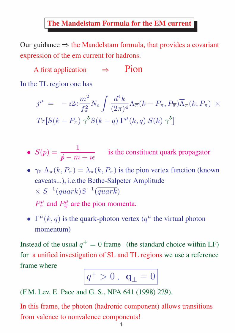
The Mandelstam Formula for the EM current

Our guidance ⇒ the Mandelstam formula, that provides a covariant

expression of the em current for hadrons.

A first application ⇒ Pion

In the TL region one has

jµ = − ı2em2

f2π

Nc

∫d4k

(2π)4Λπ(k − Pπ, Pπ)Λπ(k, Pπ) ×

Tr[S(k − Pπ) γ5S(k − q) Γµ(k, q) S(k) γ5]

• S(p) =1

/p−m+ ıǫis the constituent quark propagator

• γ5 Λπ(k, Pπ) = λπ(k, Pπ) is the pion vertex function (known

caveats...), i.e.the Bethe-Salpeter Amplitude

× S−1(quark)S−1(quark)

Pµπ and Pµ

π are the pion momenta.

• Γµ(k, q) is the quark-photon vertex (qµ the virtual photon

momentum)

Instead of the usual q+ = 0 frame (the standard choice within LF)

for a unified investigation of SL and TL regions we use a reference

frame where

q+ > 0 , q⊥ = 0

(F.M. Lev, E. Pace and G. S., NPA 641 (1998) 229).

In this frame, the photon (hadronic component) allows transitions

from valence to nonvalence components!4

Projecting out the Mandelstam Formula onto the Light Front

...through the k− integration. Only the poles of the Dirac

propagators are considered in the k− integration. We proved in a

simple model that our reference frame is the best one for this

approximation.

LF-time flows from R→ L

Timelike region

�

γ∗

Pπ

Pπ

=

�

k

Pπ

Pπ

×

k − Pπk − q

γ∗(a)

+

k − q

Pπ

Pπ

×

k − Pπ k

γ∗

(b)

(•=val)↑

0 < k+ < P+π

(� =nonval)↑P+

π< k+ < q+

× ⇒ k on its mass shell : k−on = (m2 + k2⊥)/k+

Spacelike region

�

�

P

�

P

�

0

=

�

�

P

�

P

�

0

k + P

�

�

k � q

k

(a)

+

�

�

P

�

P

�

0

+

k + P

�

k � q

k

(b)

↑(•=val)

↑(� =nonval)

↑

0 < k+ + P+π< P+

πP+

π< k+ + P+

π< P+

π′

5

⋆ First Problem: How to describe the amplitude for the emission or

absorption of a pion by a quark, � (non valence vertex), and the

qq-pion vertex, • (valence vertex)

The non valence component (�) of the pion state is given by the

emission (absorption) of a pion by a quark, we assume a constant

interaction [Choi & Ji (PLB 513 (2001) 330)]. The coupling

constant is fixed by the normalization of the pion form factor.

In the valence sector 0 < k+ < P+π ( • ), we relate the pion vertex

function Λπ(k, Pπ) to the pion Light-Front wave function

ψπ(k+,k⊥;P

+π ,Pπ⊥) =

m

fπ

P+π [Λπ(k, Pπ)][k−=k−

on]

[m2π −M2

0 (k+,k⊥;P

+π ,Pπ⊥)]

⋆⋆ Second Problem: How to model the quark-photon vertex ?

�

�

�

= �

n

8

>

>

>

>

>

>

>

>

>

>

>

>

>

>

>

>

>

>

>

>

<

>

>

>

>

>

>

>

>

>

>

>

>

>

>

>

>

>

>

>

>

:

�

�

V

n

9

>

>

>

>

>

>

>

>

>

>

>

>

>

>

>

>

>

>

>

>

>

=

>

>

>

>

>

>

>

>

>

>

>

>

>

>

>

>

>

>

>

>

>

;

⋆ When a qq pair is produced, a microscopical Vector Meson

Dominance model has been adopted.

6

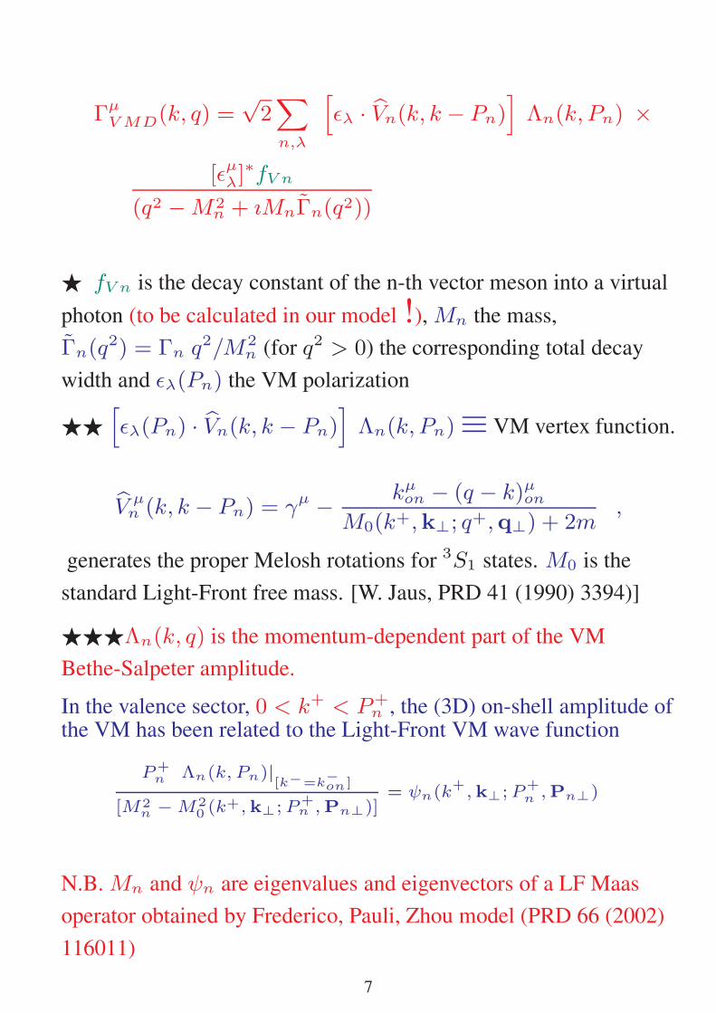
ΓµV MD(k, q) =

√2∑

n,λ

[ǫλ · Vn(k, k − Pn)

]Λn(k, Pn) ×

[ǫµλ]∗fV n

(q2 −M2n + ıMnΓn(q2))

⋆ fV n is the decay constant of the n-th vector meson into a virtual

photon (to be calculated in our model !), Mn the mass,

Γn(q2) = Γn q

2/M2n (for q2 > 0) the corresponding total decay

width and ǫλ(Pn) the VM polarization

⋆⋆

[ǫλ(Pn) · Vn(k, k − Pn)

]Λn(k, Pn)≡ VM vertex function.

V µn (k, k − Pn) = γµ − kµon − (q − k)µon

M0(k+,k⊥; q+,q⊥) + 2m,

generates the proper Melosh rotations for 3S1 states. M0 is the

standard Light-Front free mass. [W. Jaus, PRD 41 (1990) 3394)]

⋆⋆⋆Λn(k, q) is the momentum-dependent part of the VM

Bethe-Salpeter amplitude.

In the valence sector, 0 < k+ < P+n , the (3D) on-shell amplitude of

the VM has been related to the Light-Front VM wave function

P+n

Λn(k, Pn)|[k−=k−on]

[M2n−M2

0 (k+,k⊥;P+

n ,Pn⊥)]= ψn(k

+,k⊥;P+

n,Pn⊥)

N.B. Mn and ψn are eigenvalues and eigenvectors of a LF Maas

operator obtained by Frederico, Pauli, Zhou model (PRD 66 (2002)

116011)

7

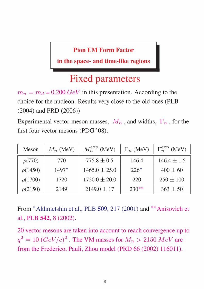
Pion EM Form Factor

in the space- and time-like regions

Fixed parameters

mu = md = 0.200 GeV in this presentation. According to the

choice for the nucleon. Results very close to the old ones (PLB

(2004) and PRD (2006))

Experimental vector-meson masses, Mn , and widths, Γn , for the

first four vector mesons (PDG ’08).

Meson Mn (MeV) Mexpn (MeV) Γn (MeV) Γexp

n (MeV)

ρ(770) 770 775.8 ± 0.5 146.4 146.4 ± 1.5

ρ(1450) 1497∗ 1465.0 ± 25.0 226∗ 400 ± 60

ρ(1700) 1720 1720.0 ± 20.0 220 250 ± 100

ρ(2150) 2149 2149.0 ± 17 230∗∗ 363 ± 50

From ∗Akhmetshin et al., PLB 509, 217 (2001) and ∗∗Anisovich et

al., PLB 542, 8 (2002).

20 vector mesons are taken into account to reach convergence up to

q2 = 10 (GeV/c)2 . The VM masses for Mn > 2150MeV are

from the Frederico, Pauli, Zhou model (PRD 66 (2002) 116011).

8

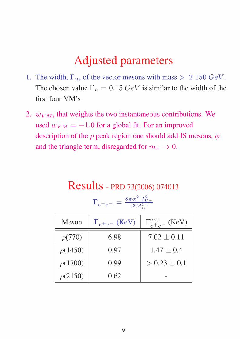
Adjusted parameters

1. The width, Γn, of the vector mesons with mass > 2.150 GeV .

The chosen value Γn = 0.15 GeV is similar to the width of the

first four VM’s

2. wV M , that weights the two instantaneous contributions. We

used wV M = −1.0 for a global fit. For an improved

description of the ρ peak region one should add IS mesons, φ

and the triangle term, disregarded for mπ → 0.

Results - PRD 73(2006) 074013

Γe+e− =8πα2 f2

V n

(3M3n)

Meson Γe+e− (KeV) Γexp

e+e−(KeV)

ρ(770) 6.98 7.02 ± 0.11

ρ(1450) 0.97 1.47 ± 0.4

ρ(1700) 0.99 > 0.23 ± 0.1

ρ(2150) 0.62 -

9

Pion EM Form Factor in the SL and TL regions

Comparison with Experimental Data

-10 -8 -6 -4 -2 0 2 4 6 8 10

q2 (GeV/c)

2

0.01

0.1

1

10

|Fπ(q

2)|

•: Compilation from R. Baldini et al. (EPJ. C11 (1999) 709, and

Refs. therein.)

�: TJLAB SL data (J. Volmer et al., PRL. 86, 1713 (2001). )

Solid line: calculation with the pion w.f. from the FPZ model for the

Bethe-Salpeter amplitude in the valence region (wV M = −1.0).

Dashed line: the same as the solid line, but with the asymptotic pionw.f. (Λπ(k;Pπ) = 1)

ψπ(k+,k⊥;P+

π,Pπ⊥) =

m

fπ

P+π

[M2π−M2

0 (k+,k⊥;P+

π ,Pπ⊥)]

10

The Nucleon EM Form Factors

The Dirac structure of the quark-nucleon vertex is suggested, as in

the case of the quark-pion vertex, by an effective Lagrangian (de

Araujo et al., PLB B478 (2001) 86)

Leff (x) =ǫabc√

2

∫d4x1 d

4x2 d4x3F(x1, x2, x3, x)

∑

τ1,τ2,τ3

×[mN α qa(x1, τ1) γ

5 qbC(x2, τ2) qc(x3, τ3) − (1− α)√

3×

qa(x1, τ1) γ5 γµ q

bC(x2, τ2) · qc(x3, τ3) (−ı ∂µ)

]ψN (x, τN )

+ ...

For the present time α = 1, i.e. no derivative coupling

Then, the Bethe-Salpeter amplitude for the nucleon can be

approximated as follows

ΦσN (k1, k2, k3, PN ) = ı

[S(k1) τy γ

5 SC(k2)C ⊗ S(k3) +

S(k3) τy γ5 SC(k1)C ⊗ S(k2) + S(k3) τy γ

5 SC(k2)C ⊗ S(k1)]

× Λ(k1, k2, k3) χτN UN (PN , σ)

with a properly symmetrized Dirac structure of the qqq-nucleon

vertex.

Λ(k1, k2, k3) describes the symmetric momentum dependence of

the vertex function upon the quark momentum variables, ki

UN (PN , σ) and χτN are the nucleon spinor and isospin eigenstate.

11

Spacelike nucleon em form factors

are evaluated from the matrix elements of the macroscopic current

〈σ′, P ′

N |jµ |PN , σ〉 = UN (P ′

N , σ′)

[−F2(Q

2)P ′

Nµ+ PN

µ

2MN+

(F1(Q

2) + F2(Q2))γµ

]UN (PN , σ)

which are approximated microscopically by the Mandelstam

formula

〈σ′, P ′

N |jµ |PN , σ〉 =∫

d4k1(2π)4

∫d4k2(2π)4

Σ{Φσ′

N (k1, k2, k′

3, P′

N )

× S−1(k1) S−1(k2) Iµ(k3, q) Φσ

N (k1, k2, k3, PN )}

3 Nc

where Iµ(k3, q) is the quark-photon vertex.

As in the pion case, we integrate on k−1 and on k−2 taking into

account only the poles of the propagators. Then we are left with a

three-momentum dependence of the vertex functions.

Frame : q⊥ = 0 q+ = |q2|1/2

Quark mass : mu = md = 200MeV . As in the case of the pion.

12

As result of the k− integrations one has

Spacelike Region

Triangle contr. Pair contr. (Z-diagr.)

�

�

P

N

P

N

0

=

�

�

P

N

P

N

0

k

1

�

k

2

�

k

3

+ q

k

3

(a)

+

�

�

P

N

P

N

0

+

k

1

k

2

�

k

3

+ q

k

3

(b)

↑(non-val.)

(val.) 0 < k+i< P

+N

0 > k+3 > −q+

× ⇒ k on the mass shell : k−on = (m2 + k2⊥)/k+

Timelike Region

�

�

P

�

N

P

N

=

�

k

3

P

�

N

P

N

�

+

k

1

k

3

+ q

k

2

�

(a)

+

�

P

�

N

P

N

�

+

k

1

k

3

k

2

k

3

+ q

�

(b)

P+N< k

+3 + q+ < q+ 0 < k

+3 + q+ < P

+N

A non-valence contribution of the photon is involved: |qqq, qqq〉13

Ansatzes for the following 3D projections of the Nucleon 4D

Bethe-Salpeter amplitude will be needed

PN

×

×

The onshell vertex function (→ valence component ), with all the

three legs as quark legs (two of them on the k−-shell)

�

PN×

Off-shell nucleon vertex in the SL region

�

PN×

Off-shell nucleon vertex in the TL region

14

Quark-Photon Vertex

Iµ = IµIS + τzIµ

IV

each term contains a purely valence contribution (in the SL region

only, θ(−Q2)) and a contribution corresponding to the pair

production (or Z-diagram).

The Z-diagram contribution can be decomposed in a bare term + a

Vector Meson Dominance term (according to the decomposition of

the photon state in bare, hadronic [and leptonic] contributions), viz

Iµi (k, q) = Ni θ(P

+N − k+) θ(k+) γµ +

+ θ(q+ + k+) θ(−k+){ZB Ni γ

µ + ZiV M Γµ[k, q, i]

}

with i = IS, IV, NIS = 1/6 and NIV = 1/2. The constants ZB

(bare term) and ZiV M (VMD term) are unknown weights to be

extracted from the phenomenological analysis of the data.

The VMD term Γµ[k, q, i] is the same already used in the pion case,

but now includes isoscalar mesons. Up to 20 IS and IV mesons

Inputs: masses, Mn , and total widths, Γn , for the first three IS

mesons. For the remaining 17, masses from FPZ model, and total

width Γn = 0.15MeV as for the IV sector. We calculate

microscopically Γie−e+ and the amplitudes VM → NN and

VM +N → N

Meson Mn (MeV) Γn (MeV)

ω 782 8.44

ω′ 1420 174

ω′′ 1720 220

15

Momentum Dependence of theBethe-Salpeter Amplitudes

In the valence vertex the spectator quarks are on their-own k−-shell,

and the momentum dependence, reduced to a 3-momentum

dependence by the k− integrations, is approximated through a

Nucleon Wave Function a la Brodsky (PQCD inspired), namely

ΨN (k1, k2, k3) = P+N

ΛV (k1, k2, k3)

[M2N −M2

0 (1, 2, 3)]=

= P+N N (9m2)7/2

(ξ1ξ2ξ3)p [β2 +M20 (1, 2, 3)]

7/2

where M0(1, 2, 3) is the free mass of the three-quark system,

ξi = k+i /P+N

and N a normalization constant.

The power 7/2 and the parameter p = 0.13 are chosen to have an

asymptotic decrease of the triangle contribution faster than the

dipole.

Only the triangle diagram determines the magnetic moments,

weakly dependent on p. Then β = 0.65 can be fixed by µp and µn

Proton: 2.87 (Exp. 2.793) Neutron : -1.85 (Exp. -1.913)

16

�

PN×

�

PN×

SL off-shell vertex TL off-shell vertex

The non-valence vertex can depend on the available invariants. in

the spacelike region, one can single out the free mass of quarks 1

and 2, M0(1, 2), and the free mass of the N-q system M0(N, 3)

Then in the spacelike region we approximate the momentum

dependence of the non-valence vertex by

ΛSLNV (k1, k2, k3) = [g12]

2 [gN 3]7/2−2

[k+12P ′+N

] [P+N

k+3

]r [P ′+N

k+3

]r

k+12 = k+1 + k+2 gAB =(mA mB)

[β2 +M20 (A,B)]

In the timelike region the non-valence vertex can depend on the

mass of the ( nucleon - diquark ) system . Then by analogy we

approximate the non-valence vertex in diagram (a) by

ΛTLNV (k1, k2, k3) = 2 [g12]

2 [gN,12]3/2

[−k+12P+N

] [P+N

k′+3

]r[P+N

k′+3

]r

An analogous expression is used for diagram (b).

17

Adjusted parameters (in the SL region)

• the weights for the pair production terms :

ZB = ZIVV M = 2.283 and

ZISV M/Z

IVV M = 1.12

• the power p = 0.13 of ξi in the valence amplitude

• the power r = 0.17 of the ratio P+N /k

+

3in the spacelike

non-valence vertex, to have a dipole asymptotic behavior of the

pair-production contribution

By using in the fitting procedure the experimental data (updated to

2009) for µpGpE/G

pM , Gn

E , GpM and Gn

M

⇒ χ2 = 1.7

Results from PLB 671, 153 (2009)

rp = (0.903± 0.004) fm rexpp = (0.895± 0.018) fm

−[dGn

E(Q2)

dQ2

]th

Q2=0

= (0.501± 0.002) (GeV/c)−2

−[dGn

E(Q2)

dQ2

]exp

Q2=0

= (0.512± 0.013) (GeV/c)−2

18

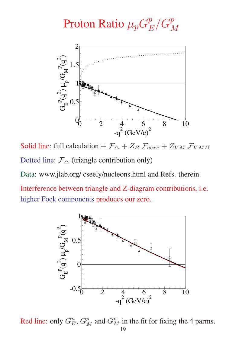
Proton Ratio µpGp

E/Gp

M

0 2 4 6 8 10

-q2 (GeV/c)

2

0

0.5

1

1.5

2

GE

p(q

2)

µ p/G

M

p(q

2)

Solid line: full calculation ≡ F△ + ZB Fbare + ZV M FV MD

Dotted line: F△ (triangle contribution only)

Data: www.jlab.org/ cseely/nucleons.html and Refs. therein.

Interference between triangle and Z-diagram contributions, i.e.

higher Fock components produces our zero.

0 2 4 6 8 10

-q2 (GeV/c)

2

-0.5

0

0.5

1

GE

p(q

2)

µ p/G

M

p(q

2)

Red line: only GnE , Gp

M and GnM in the fit for fixing the 4 parms.

19

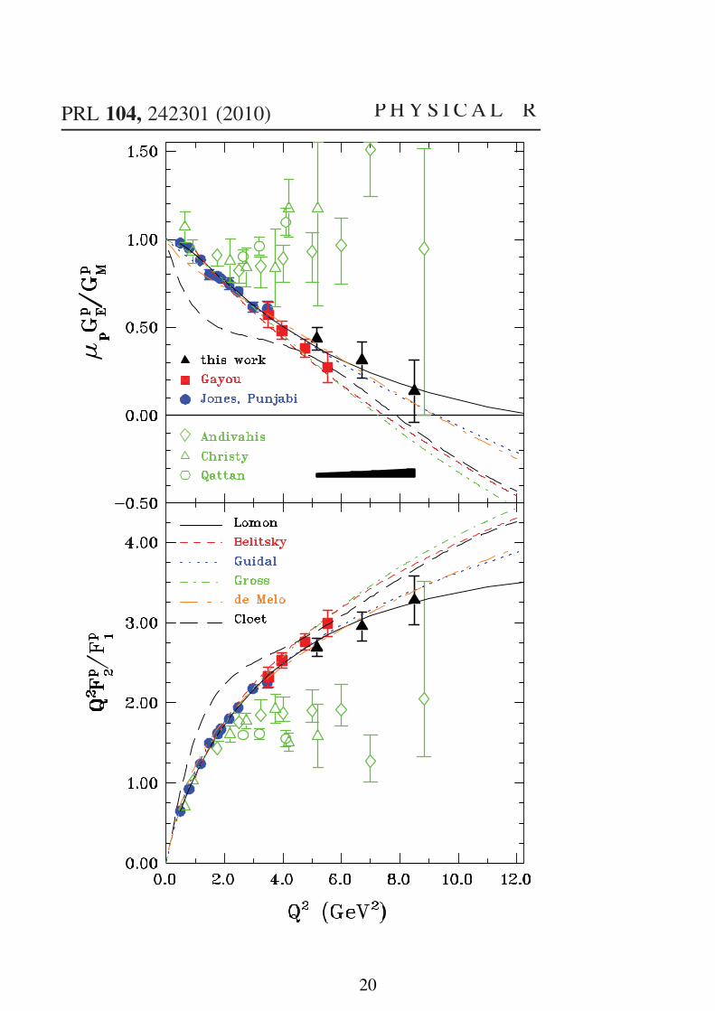
PRL 104, 242301 (2010) P HY S I CA L R EV I EW LE T T E R S

20

SL Nucleon form factors: GnE, Gp

M GnM

0 1 2

-q2

(GeV/c)2

0.00

0.05

0.10

GE

n(q

2)

Solid line: full calculation ≡ F△ + ZB Fbare + ZV M FV MD

Dotted line: F△ (triangle contribution only)

Values obtained from our model

−[dGn

E(Q2)

dQ2

]th

Q2=0

= (0.501± 0.002) (GeV/c)−2

−[dGn

E(Q2)

dQ2

]exp

Q2=0

= (0.512± 0.013) (GeV/c)−2

21

0.1 1 10

-q2

(GeV/c)2

0.4

0.6

0.8

1G

M

p(q

2)/

µ pG

D(-

q2)

0.1 1 10

-q2

(GeV/c)2

0.4

0.6

0.8

1.0

GM

n(q

2)/

µ nG

D(-

q2)

Solid line: full calculation ≡ F△ + ZB Fbare + ZV M FV MD

Dotted line: F△ (triangle contribution only)

The pair-production contribution is essential for the result

GD = 1/[1− q2/(0.71 (GeV/c)2)]2

22

Nucleon timelike form factorsParameter free results

4 6 8 10 20

q2

(GeV/c)2

0

5

10

15

20

25

Gp

eff(q

2)/

GD

(q2)

Solid line: full calculation - Dotted line: bare production (no VM).

Missing strength at q2 = 4.5 (GeV/c)2 and q2 = 8 (GeV/c)2

4 6 8 10

q2

(GeV/c)2

0

5

10

15

20

25

Gn

eff(q

2)/

GD

(q2)

Dashed line: solid line arbitrarily × 2.

Geff (q2) =

√2τ |GM (q2)|2 + |GE(q2)|2

2τ + 1

23

Polarization orthogonal to the scattering plane: no polarized beam !

Py(θCM ) = − sin (2θCM )ℑ{GE(q

2)G∗

M (q2)}D

√τ

where τ = q2/4M2 and

D =[

1 + cos2 (θCM )]

|GM (q2)|2 + sin2 (θCM )|GE(q2)|2

τ

5 10 15 20 25 30 35 40

q2 (GeV/c)

2

-0.4

-0.2

0

0.2

0.4

Py(4

5o)

Py proton

Py neutron

LF Constituent Quark

Model

-0.4

-0.2

0

0.2

0.4

5 10 15 20 25 30 35 40

1/Q fit

(log2 Q2) /Q2 fit

impr. (log2 Q2) /Q2 fitIJL fit

Pol

ariz

atio

n P

y (fo

r θ

= 4

5°)

q2 (GeV2)

After Brodsky, Carlson,

Hiller and Dae Sung

Hwang PRD 69, 054022

(2004).

24

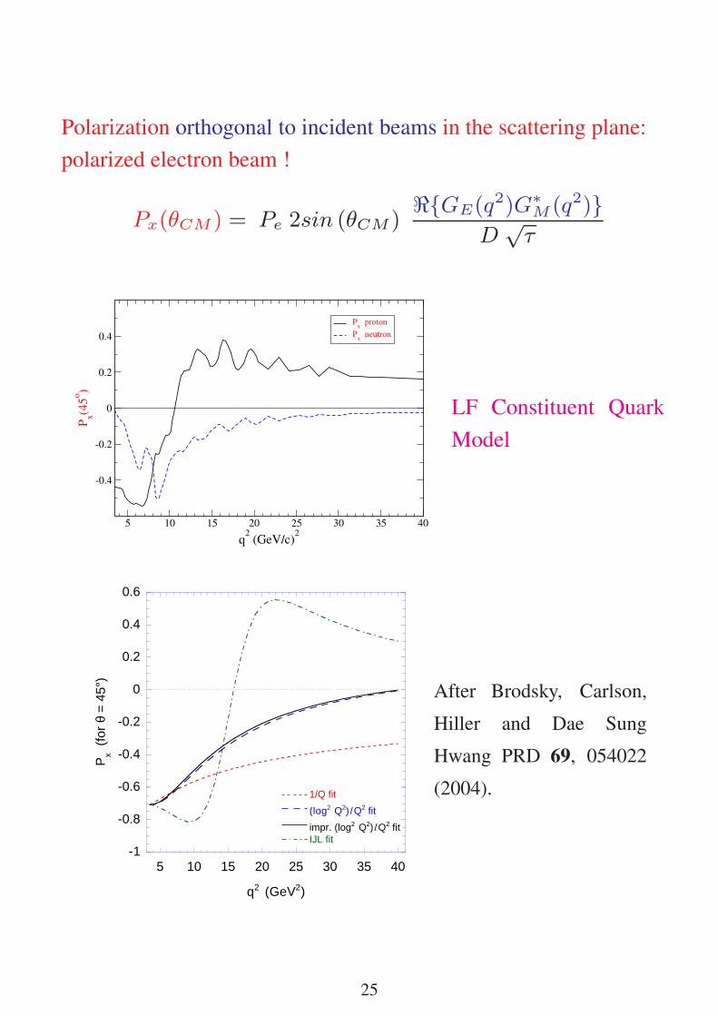
Polarization orthogonal to incident beams in the scattering plane:

polarized electron beam !

Px(θCM ) = Pe 2sin (θCM )ℜ{GE(q

2)G∗

M (q2)}D

√τ

5 10 15 20 25 30 35 40

q2 (GeV/c)

2

-0.4

-0.2

0

0.2

0.4

Px(4

5o)

Px proton

Px neutron

LF Constituent Quark

Model

-1

-0.8

-0.6

-0.4

-0.2

0

0.2

0.4

0.6

5 10 15 20 25 30 35 40

1/Q fit

(log2 Q2) /Q2 fit

impr. (log2 Q2) /Q2 fitIJL fit

Px (

for

θ =

45°

)

q2 (GeV2)

After Brodsky, Carlson,

Hiller and Dae Sung

Hwang PRD 69, 054022

(2004).

25

Polarization along the incident beams: polarized electron beam !

Pz(θCM ) = Pe 2cos (θCM )|GM (q2)|2

D

5 10 15 20 25 30 35 40

q2 (GeV/c)

2

0

0.2

0.4

Pz(4

5o)

Pz proton

Pz neutron

LF Constituent Quark

Model

0

0.2

0.4

0.6

0.8

1

5 10 15 20 25 30 35 40

1/Q fit

(log2 Q2) /Q2 fit

impr. (log2 Q2) /Q2 fitIJL fit

Pz (

for

θ =

45°

)

q2 (GeV2)

After Brodsky, Carlson,

Hiller and Dae Sung

Hwang PRD 69, 054022

(2004).

26

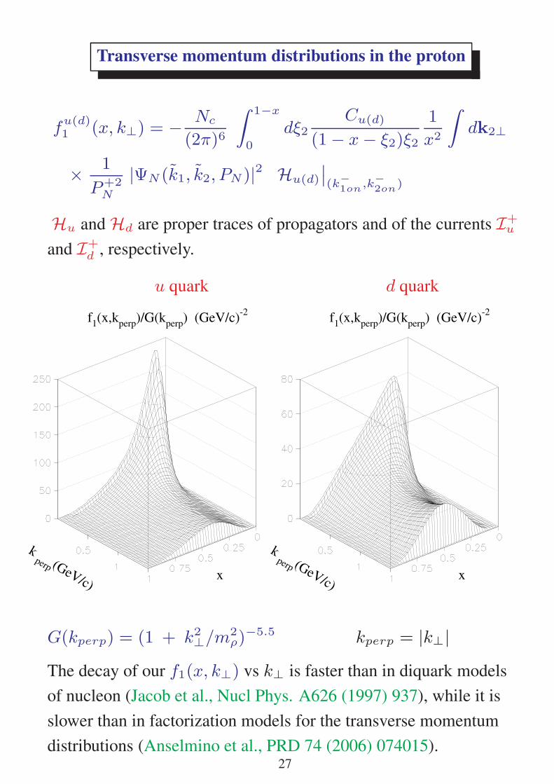
Transverse momentum distributions in the proton

fu(d)1 (x, k⊥) = − Nc

(2π)6

∫ 1−x

0

dξ2Cu(d)

(1− x− ξ2)ξ2

1

x2

∫dk2⊥

× 1

P+2N

|ΨN (k1, k2, PN )|2 Hu(d)

∣∣(k−

1on,k−

2on)

Hu and Hd are proper traces of propagators and of the currents I+u

and I+d , respectively.

u quark d quark

k perp (GeV/c)

x

f1(x,k

perp)/G(k

perp) (GeV/c)

-2

k perp (GeV/c)

x

f1(x,k

perp)/G(k

perp) (GeV/c)

-2

G(kperp) = (1 + k2⊥/m2ρ)

−5.5 kperp = |k⊥|The decay of our f1(x, k⊥) vs k⊥ is faster than in diquark models

of nucleon (Jacob et al., Nucl Phys. A626 (1997) 937), while it is

slower than in factorization models for the transverse momentum

distributions (Anselmino et al., PRD 74 (2006) 074015).27

Longitudinal momentum distributions

For P ′

N = PN the unpolarized GPD Hq(x, ξ, t) reduces to the

longitudinal parton distribution function q(x)

Hq(x, 0, 0) =

∫dz−

4πeixP

+N

z− 〈PN |ψq(0) γ+ ψq(z)|PN 〉

∣∣z=0

= q(x) =

∫dk⊥ fq

1 (x, k⊥)

an average on the nucleon helicities is understood.

proton preliminary results

u quark d quark

0 0.2 0.4 0.6 0.8 1x

0

0.5

1

1.5

x u

val

(x)

0 0.2 0.4 0.6 0.8 1x

0

0.5

1

x d

val

(x)

Dashed lines : our longitudinal momentum distributions

Thick solid lines : our model after evolution to Q2 = 1.6 (GeV/c)2

Thin solid lines : CTEQ4 fit to data [Lai et al., PRD 51 (1995) 4753]

28

Conclusions & Perspectives

• A relativistic Constituent Quark Model, based on

phenomenological Ansatzes for the hadron Bethe-Salpeter

amplitudes, have been applied for evaluating both pion and

nucleon em form factors, in SL and TL regions.

• A microscopical Vector Meson Dominance model has been

devised, exploiting masses and eigenfunction of a relativistic

mass operator, able to reproduce the vector meson mass in

PDG 08.

• Only 4 adjusted paramters are necessary to get χ2 ∼ 1.7 in the

SL region for the nucleon ff.

• It is predicted a zero for the SL ratio µpGpE/G

pM around

Q2 ∼ 9 (GeV/c)2. The interference between the valence and

non valence component (pair production) of the proton state is

the cause. Notice that the whole µpGpE/G

pM should be

considered a prediction.

• TL Nucleon ff are true predictions!

• The comparison with experimental data for the proton points to

missing strength around 4.5 and 8 (GeV/c)2

• Fenice data for the neutron ff is largely underestimated

• Calculations of the TL polarizations show interesting

structures, related both to the realistic description of the SL

nucleon ff’s and to the VMD

• Extension to TMD and GPD is currently under progress. Pion

done29

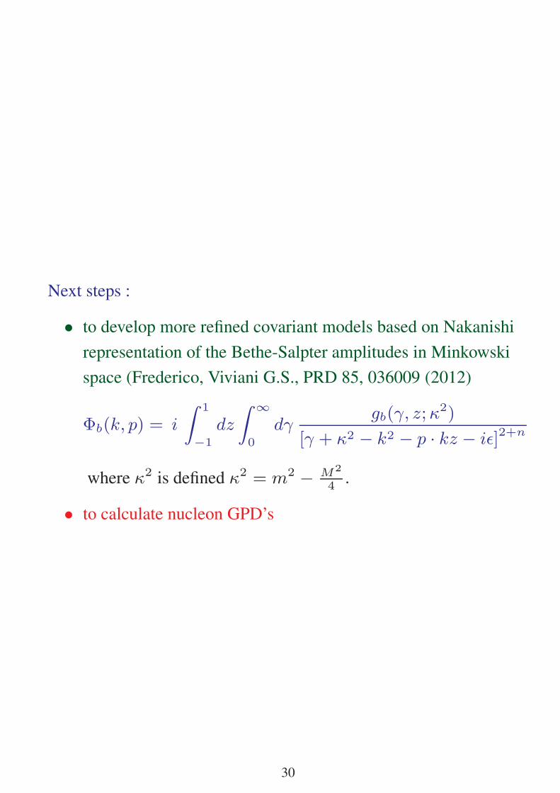
Next steps :

• to develop more refined covariant models based on Nakanishi

representation of the Bethe-Salpter amplitudes in Minkowski

space (Frederico, Viviani G.S., PRD 85, 036009 (2012)

Φb(k, p) = i

∫ 1

−1

dz

∫∞

0

dγgb(γ, z;κ

2)

[γ + κ2 − k2 − p · kz − iǫ]2+n

where κ2 is defined κ2 = m2 − M2

4.

• to calculate nucleon GPD’s

30