the limits of earth orbital calculations for geological time-scale use

The limits of Earth orbital calculations forgeological time-scale use

By Jacques Laskar

Astronomie et Systemes Dynamiques, CNRS–Bureau des Longitudes,77 Av. Denfert-Rochereau, 75014 Paris, France

The orbital motion of the planets in the Solar System is chaotic. As a result, initiallyclose orbits diverge exponentially with a characteristic Lyapunov time of 5 Ma. Thissensitivity to initial conditions will limit the possibility of obtaining an accuratesolution for the orbital and precessional motion of the Earth over more than 35–50 Ma. The principal sources of uncertainty in the model are reviewed here. It appearsthat at present the largest source of error could reside in the lack of knowledge of thevalue of the precession due to the oblateness (J2) of the Sun. Nevertheless, for thecalibration of geological time-scale, this limitation can be overcome to some extentif one considers in the geological data the signature of the outer planets’ secularorbital motion which is predictable on a much longer time-scale. Moreover, it shouldbe possible to observe in the geological records the trace of transition from the(s4 − s3)− 2(g4 − g3) secular resonance to the (s4 − s3)− (g4 − g3) resonance. Thedetection and dating of these passages should induce extremely high constraints onthe dynamical models for the orbital evolution of the Solar System.

Keywords: precession; obliquity; orbital evolution; chaos;Solar System; Milankovitch cycles; palaeoclimates

1. Introduction

The insolation at a given point on Earth depends on the position of the Earth inspace, and on the orientation of the Earth relative to the Sun. In order to makeprecise computations of the past climatic evolution of the Earth, one thus needsfirst to have an accurate solution for the orbital evolution of the Earth, and then tocompute the evolution of the orientation of the axis of the Earth.

The orbital computation is a difficult task since the Earth’s motion is perturbedby all the other planets of the Solar System. The first approximate solution of thisproblem was given by Le Verrier (1856), and was used by Milankovitch for his studieson the astronomical origin of the ice ages. Le Verrier’s solution consisted of linearizedequations for the mean evolution of the orbits of the planets. It was completed lateron by Hill (1897), who recognized that higher-order terms, coming from the mutualinteractions of Jupiter and Saturn, can significantly change the solution of Le Verrier.The solution of Brouwer & Van Woerkom (1950) is essentially that of Le Verrier, withthe addition of the terms computed by Hill. It provides a solution which representsin a very reasonable way the evolution of the orbit of the Earth over a few hundredthousand years, and was used for insolation computations by Sharav & Boudnikova(1967a, b) with updated values of the parameters. The next major improvement wasgiven by Bretagnon (1974), who computed terms of second order and degree 3 in the

Phil. Trans. R. Soc. Lond. A (1999) 357, 1735–1759Printed in Great Britain 1735

c© 1999 The Royal SocietyTEX Paper

1736 J. Laskar

secular (mean) equations. This solution was then used by Berger (1976, 1978) forthe computation of the precession and insolation quantities for the Earth followingSharav & Boudnikova (1967a, b). All of these solutions assumed implicitly that themotion of the Solar System is regular, and that the solution could thus be obtainedas quasi-periodic series, using perturbation theory.

In Laskar (1984, 1985, 1986), I computed in an extensive way the secular equationsgiving the mean motion of the whole Solar System, including all terms up to order2 with respect to the masses, and up to degree 5 in the eccentricity and inclinationof the planets (thus also including all the terms of Hill). It was clear from thesecomputations that the assumed practical convergence of the perturbative series wasvain, and strong evidence of divergence becomes apparent in the system of the innerplanets (Laskar 1984).

This difficulty was overcome by a numerical integration of the secular (i.e. aver-aged) equations, which could be performed in a very efficient way, using a stepsize of500 years. The outcome of these computations was to provide a much more accuratesolution for the orbital evolution of the Solar System (Laskar 1986, 1988), which alsoincluded a full solution of obliquity and precession usable for insolation computation.But at the same time, I demonstrated the chaotic behaviour of the orbits of the plan-ets of the Solar System, and more specifically of the inner planets, thus destroyingthe hope of obtaining an astronomical solution to use to develop a palaeoclimatetime-scale for the Earth over several hundreds of millions of years (Laskar 1989).

Later on, and shortly after the publication of the direct numerical integration over3 Ma of Quinn et al . (1991), we published an improved solution for the precessionand obliquity solution, aimed to help palaeoclimate computation over 20 Ma (Laskaret al . 1993a). This solution was made widely available through the Internet (requestsfor these files should be addressed to [email protected]), together with a set of routinesallowing changes to the model of precession. This solution was limited to 20 Ma,that is the time span over which we assumed that the exponential divergence dueto chaotic behaviour was not sensitive. Due to the improvement of the geologicaltechniques, several groups are now studying sedimentary cores extending over morethan 20 Ma, and there is a demand for astronomical solutions extending further intime. This requires a closer look at the real precision of the solutions, and the aimof the present paper is to clarify this point, by setting more precise bounds on thelimits of Earth orbital calculations for geological time-scale use.

2. Chaotic motion of the Solar System

The main result from the long-term integration of the secular Solar System equationswas the discovery that the full Solar System, and especially the inner Solar System ischaotic (Laskar 1989) with a Lyapunov time of ca. 5 Ma. This means that the distanceof two planetary solutions, starting in the phase space with a distance d(0) = d0,evolves approximately as†

d(T ) ≈ d0eT/5, (2.1)

† The distance here corresponds to the variables used in the integration of the problem, which areeither similar to an eccentricity, or to an inclination. In both cases, if the inclinations are expressed inradians, they are relative distances in physical space, but for an easier comparison of the results for theinclinations, we prefer to use degrees in the figures instead of radians.

Phil. Trans. R. Soc. Lond. A (1999)

Limits of Earth orbital calculations 1737

or, in a more straightforward way, and which is even closer to the true value,

d(T ) ≈ d010T/10, (2.2)

where T is expressed in millions of years. Following this formula, an initial error of10−10 leads to an indeterminacy of ≈ 10−9 after 10 Ma, but reaches the order of 1after 100 Ma. From these results, it was clear that the planetary solutions can be veryaccurate for 10–20 Ma, and probably irrelevant for precise predictions after 100 Ma.

Nevertheless, the Lyapunov time of 5 Ma, which is given here, is a global constantfor the whole Solar System. This is valid, as due to coupling, all solutions will undergothe effects of the chaotic component; but as this coupling is small, the effect on someof the planets could also be small over a limited time span.

For the practical purpose of calibrating the astronomical time-scale for the terres-trial sediments, it is thus necessary to look more closely at the specific solution of theEarth’s orbital elements. This is done in the present work through several numericalexperiments.

(a) Experiment 1

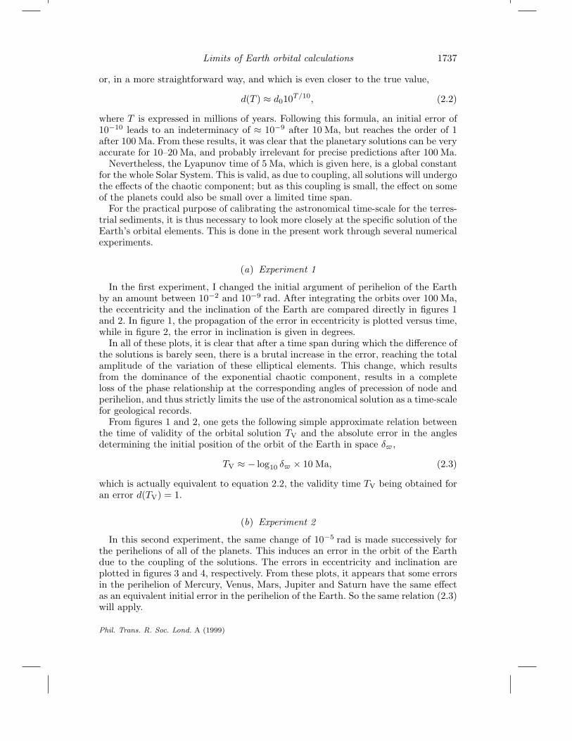
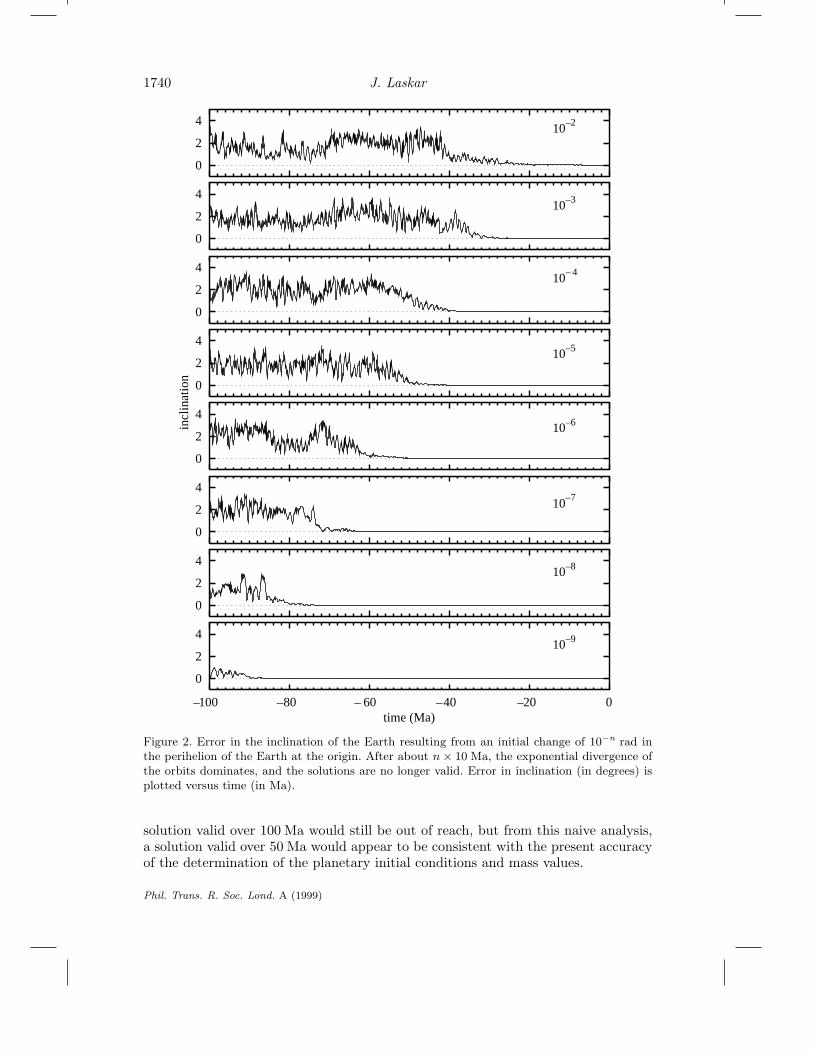
In the first experiment, I changed the initial argument of perihelion of the Earthby an amount between 10−2 and 10−9 rad. After integrating the orbits over 100 Ma,the eccentricity and the inclination of the Earth are compared directly in figures 1and 2. In figure 1, the propagation of the error in eccentricity is plotted versus time,while in figure 2, the error in inclination is given in degrees.

In all of these plots, it is clear that after a time span during which the difference ofthe solutions is barely seen, there is a brutal increase in the error, reaching the totalamplitude of the variation of these elliptical elements. This change, which resultsfrom the dominance of the exponential chaotic component, results in a completeloss of the phase relationship at the corresponding angles of precession of node andperihelion, and thus strictly limits the use of the astronomical solution as a time-scalefor geological records.

From figures 1 and 2, one gets the following simple approximate relation betweenthe time of validity of the orbital solution TV and the absolute error in the anglesdetermining the initial position of the orbit of the Earth in space δ$,

TV ≈ − log10 δ$ × 10 Ma, (2.3)

which is actually equivalent to equation 2.2, the validity time TV being obtained foran error d(TV) = 1.

(b) Experiment 2

In this second experiment, the same change of 10−5 rad is made successively forthe perihelions of all of the planets. This induces an error in the orbit of the Earthdue to the coupling of the solutions. The errors in eccentricity and inclination areplotted in figures 3 and 4, respectively. From these plots, it appears that some errorsin the perihelion of Mercury, Venus, Mars, Jupiter and Saturn have the same effectas an equivalent initial error in the perihelion of the Earth. So the same relation (2.3)will apply.


1738 J. Laskar

For Uranus and Neptune, the induced error is not so large, and we can see an offsetof 30 Ma with respect to the previous relation. The time of validity of the orbit willthus be something more like

TV ≈ − log10(10−3δ$)× 10 Ma, (2.4)

which means that for Uranus and Neptune we can accept an error 1000 times largerthan that for the other planets.

(c) Experiment 3

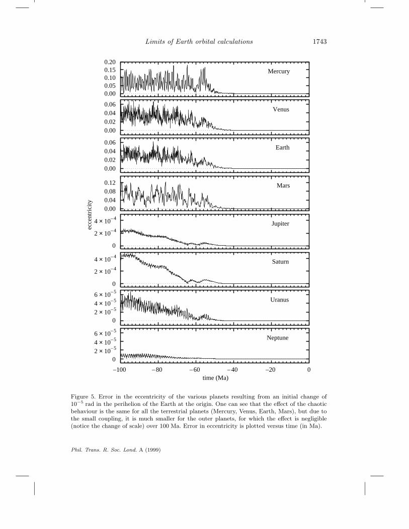
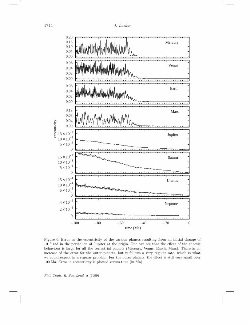
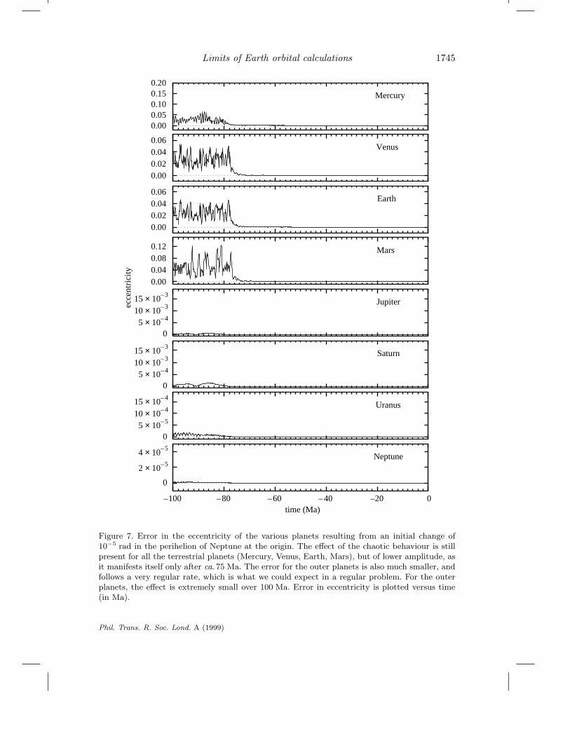
Here we start with an offset in the orbit of one of the planets, and examine theresulting effect for the solution of all the other planets. This is done successively forthe Earth (figure 5), Jupiter (figure 6), and Neptune (figure 7). For brevity, only theresults for eccentricity are plotted, but the results for inclination are very similar.

It is quite clear that all the inner planets have the same chaotic behaviour, whileall of the solutions for the outer planets behave much more regularly. There are stillsome chaotic effects, especially in figure 5, but the resulting error over 100 Ma is stillvery small. With an initial error for an outer planet (figures 6 and 7), the errors inthe outer planets grow regularly and do not show exponential trends over 100 Ma.

(d) Conclusions

From these computations, it appears clearly that the solution for the Earth fol-lows strictly the exponential relations given in (2.1) and (2.2), and that the time ofvalidity for the orbital solution will be given by the relation (2.3). These numericalexperiments will now be used to estimate the propagated error due to the uncertaintyin the initial conditions and parameters of the model.

3. Constants of the planetary solution

If one sets aside the problems due to the model, the accuracy of the orbital solutiondepends on the planetary masses and on the precision of the initial positions and thedetermination of velocities.

(a) Planetary masses

The precision with which masses are known has been greatly improved by theVoyager Spacecraft missions, and the latest values for the planetary masses are givenin table 1. The uncertainties are obtained from the latest adjustment of the JPLephemeris DE405 (Standish 1998).

(b) Planetary positions

The uncertainty of the observations for the positions of the planets should bebetter than 0.1′′ ≈ 0.5×10−6 rad, and this will not be a limiting factor for obtaininga solution over an extended time span.

If we assume in general a precision of 10−6 for the planetary masses and positions,using the relation (2.3), one sees that the maximum validity time for the orbitalsolution will be

TV ≈ 60 Ma. (3.1)



00.020.040.06

ecce

ntri

city

10

00.020.040.06

10

00.020.040.06

10

00.020.040.06

10

00.020.040.06

10

00.020.040.06

10

00.020.040.06

10

00.020.040.06

100 80 60time (Ma)

–9

–8

–7

–6

–5

–3

–2

– 4

40 20––––– 0

10

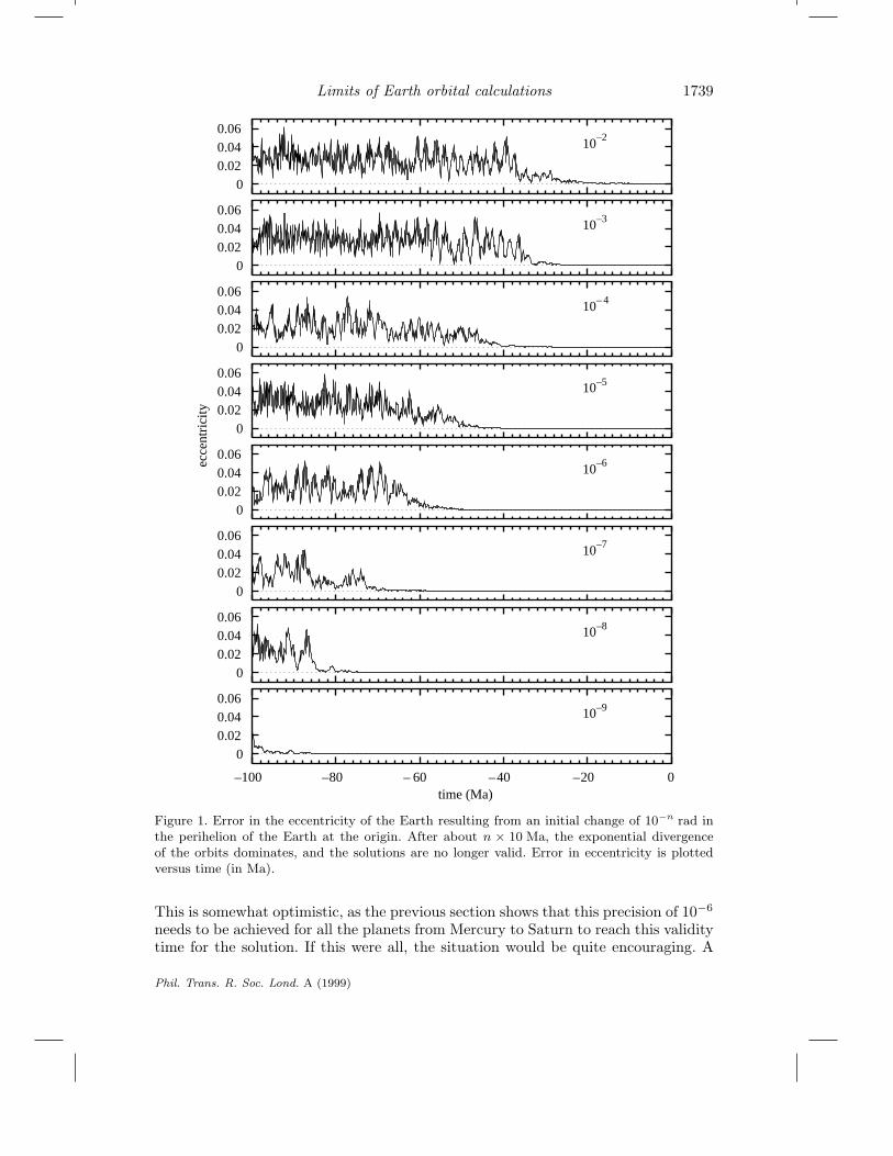
Figure 1. Error in the eccentricity of the Earth resulting from an initial change of 10−n rad inthe perihelion of the Earth at the origin. After about n × 10 Ma, the exponential divergenceof the orbits dominates, and the solutions are no longer valid. Error in eccentricity is plottedversus time (in Ma).

This is somewhat optimistic, as the previous section shows that this precision of 10−6

needs to be achieved for all the planets from Mercury to Saturn to reach this validitytime for the solution. If this were all, the situation would be quite encouraging. A


1740 J. Laskar

0

2

4

incl

inat

ion

0

2

4

0

2

4

0

2

4

0

2

4

0

2

4

0

2

4

0

2

4

100 80 60time (Ma)

40 20 0–––––

10

10

10

10

10

10

10

–9

–8

–7

–6

–5

–3

–2

– 4

10

Figure 2. Error in the inclination of the Earth resulting from an initial change of 10−n rad inthe perihelion of the Earth at the origin. After about n× 10 Ma, the exponential divergence ofthe orbits dominates, and the solutions are no longer valid. Error in inclination (in degrees) isplotted versus time (in Ma).

solution valid over 100 Ma would still be out of reach, but from this naive analysis,a solution valid over 50 Ma would appear to be consistent with the present accuracyof the determination of the planetary initial conditions and mass values.



00.020.040.06

ecce

ntri

city

Mercury

00.020.040.06

Venus

00.020.040.06

Earth

00.020.040.06

Mars

00.020.040.06

Jupiter

00.020.040.06

Saturn

00.020.040.06

Uranus

00.020.040.06

100 80 60time (Ma)

40 20 0–––––

Neptune

Figure 3. Error in the eccentricity of the Earth resulting from an initial change of 10−5 rad inthe perihelion of the various planets at the origin. It is clear that an error in the position ofMercury, Venus, Mars, Jupiter, Saturn, has the same impact as the same error in the perihelionof the Earth. For Uranus and Neptune, due to the smaller coupling, the error becomes importantonly 30 Ma later. Error in eccentricity is plotted versus time (in Ma).


1742 J. Laskar

0

2

4

incl

inat

ion

Mercury

0

2

4Venus

0

2

4Earth

0

2

4Mars

0

2

4Jupiter

0

2

4Saturn

0

2

4Uranus

0

2

4

100 80 60 40time (Ma)

20––––– 0

Neptune

Figure 4. Error in the inclination of the Earth resulting from an initial change of 10−5 rad in theperihelion of the various planets at the origin. It is clear that an error in the position of Mercury,Venus, Mars, Jupiter, Saturn, has the same impact as the same error in the perihelion of theEarth. For Uranus and Neptune, due to the smaller coupling, the error becomes important only30 Ma later. Error in inclination (in degrees) is plotted versus time (in Ma).



0.000.050.100.150.20

ecce

ntri

city

Mercury

0.000.020.040.06

Venus

0.000.020.040.06

Earth

0.00

4 × 10 4–

2 × 10 4–

0

4 × 10 4–

2 × 10 4–

0

4 × 10 5–6 × 10 5–

2 × 10 5–

0

4 × 10 5–6 × 10 5–

2 × 10 5–

0

0.040.080.12 Mars

Jupiter

Saturn

Uranus

100 80–– – – –60 40time (Ma)

20 0

Neptune

Figure 5. Error in the eccentricity of the various planets resulting from an initial change of10−5 rad in the perihelion of the Earth at the origin. One can see that the effect of the chaoticbehaviour is the same for all the terrestrial planets (Mercury, Venus, Earth, Mars), but due tothe small coupling, it is much smaller for the outer planets, for which the effect is negligible(notice the change of scale) over 100 Ma. Error in eccentricity is plotted versus time (in Ma).


1744 J. Laskar

0.000.050.100.150.20

Mercury

0.000.020.040.06

Venus

0.000.020.040.06

Earth

0.000.040.080.12 Mars

Jupiter

Saturn

Uranus

Neptune

ecce

ntri

city

10 × 10 4–15 × 10 4–

5 × 10 5–

0

10 × 10 3–15 × 10 3–

5 × 10 4–

0

10 × 10 3–15 × 10 3–

5 × 10 4–

0

4 × 10 5–

2 × 10 5–

0

100 80–– – – –60 40time (Ma)

20 0

Figure 6. Error in the eccentricity of the various planets resulting from an initial change of10−5 rad in the perihelion of Jupiter at the origin. One can see that the effect of the chaoticbehaviour is large for all the terrestrial planets (Mercury, Venus, Earth, Mars). There is anincrease of the error for the outer planets, but it follows a very regular rate, which is whatwe could expect in a regular problem. For the outer planets, the effect is still very small over100 Ma. Error in eccentricity is plotted versus time (in Ma).



0.000.050.100.150.20

Mercury

0.000.020.040.06

Venus

0.000.020.040.06

Earth

0.000.040.080.12 Mars

Jupiter

Saturn

Uranus

Neptune

ecce

ntri

city

10 × 10 4–15 × 10 4–

5 × 10 5–

0

10 × 10 3–15 × 10 3–

5 × 10 4–

0

10 × 10 3–15 × 10 3–

5 × 10 4–

0

4 × 10 5–

2 × 10 5–

0

100 80–– – – –60 40time (Ma)

20 0

Figure 7. Error in the eccentricity of the various planets resulting from an initial change of10−5 rad in the perihelion of Neptune at the origin. The effect of the chaotic behaviour is stillpresent for all the terrestrial planets (Mercury, Venus, Earth, Mars), but of lower amplitude, asit manifests itself only after ca. 75 Ma. The error for the outer planets is also much smaller, andfollows a very regular rate, which is what we could expect in a regular problem. For the outerplanets, the effect is extremely small over 100 Ma. Error in eccentricity is plotted versus time(in Ma).


1746 J. Laskar

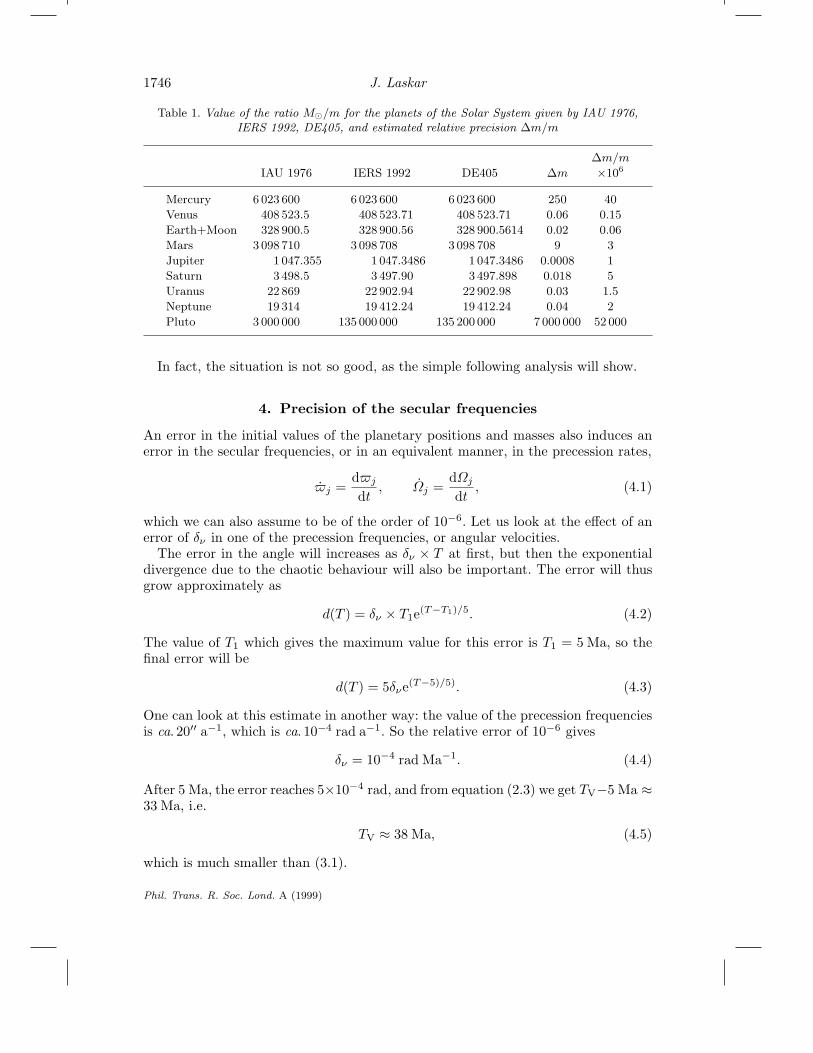
Table 1. Value of the ratio M/m for the planets of the Solar System given by IAU 1976,IERS 1992, DE405, and estimated relative precision ∆m/m

∆m/mIAU 1976 IERS 1992 DE405 ∆m ×106

Mercury 6 023 600 6 023 600 6 023 600 250 40Venus 408 523.5 408 523.71 408 523.71 0.06 0.15Earth+Moon 328 900.5 328 900.56 328 900.5614 0.02 0.06Mars 3 098 710 3 098 708 3 098 708 9 3Jupiter 1 047.355 1 047.3486 1 047.3486 0.0008 1Saturn 3 498.5 3 497.90 3 497.898 0.018 5Uranus 22 869 22 902.94 22 902.98 0.03 1.5Neptune 19 314 19 412.24 19 412.24 0.04 2Pluto 3 000 000 135 000 000 135 200 000 7 000 000 52 000

In fact, the situation is not so good, as the simple following analysis will show.

4. Precision of the secular frequencies

An error in the initial values of the planetary positions and masses also induces anerror in the secular frequencies, or in an equivalent manner, in the precession rates,

$j =d$j

dt, Ωj =

dΩjdt

, (4.1)

which we can also assume to be of the order of 10−6. Let us look at the effect of anerror of δν in one of the precession frequencies, or angular velocities.

The error in the angle will increases as δν × T at first, but then the exponentialdivergence due to the chaotic behaviour will also be important. The error will thusgrow approximately as

d(T ) = δν × T1e(T−T1)/5. (4.2)

The value of T1 which gives the maximum value for this error is T1 = 5 Ma, so thefinal error will be

d(T ) = 5δνe(T−5)/5). (4.3)

One can look at this estimate in another way: the value of the precession frequenciesis ca. 20′′ a−1, which is ca. 10−4 rad a−1. So the relative error of 10−6 gives

δν = 10−4 rad Ma−1. (4.4)

After 5 Ma, the error reaches 5×10−4 rad, and from equation (2.3) we get TV−5 Ma ≈33 Ma, i.e.

TV ≈ 38 Ma, (4.5)

which is much smaller than (3.1).



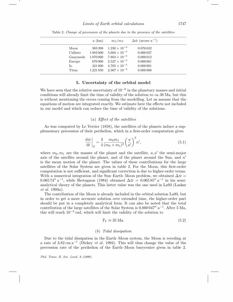
Table 2. Change of precession of the planets due to the presence of the satellites

a (km) mS/mP ∆$ (arcsec a−1)

Moon 383 398 1.230× 10−2 0.076 632Callisto 1 883 000 5.668× 10−5 0.000 027Ganymede 1 070 000 7.804× 10−5 0.000 012Europe 670 900 2.527× 10−5 0.000 001Io 421 600 4.705× 10−5 0.000 001Titan 1 221 850 2.367× 10−4 0.000 006

5. Uncertainty of the orbital model

We have seen that the relative uncertainty of 10−6 in the planetary masses and initialconditions will already limit the time of validity of the solution to ca. 38 Ma, but thisis without mentioning the errors coming from the modelling. Let us assume that theequations of motion are integrated exactly. We estimate here the effects not includedin our model and which can reduce the time of validity of the solutions.

(a) Effect of the satellites

As was computed by Le Verrier (1858), the satellites of the planets induce a sup-plementary precession of their perihelion, which in a first-order computation gives

d$dt

∣∣∣∣S

=34

m0m1

(m0 +m1)2

(a

a′

)2

n′, (5.1)

where m0,m1 are the masses of the planet and the satellite, a, a′ the semi-majoraxis of the satellite around the planet, and of the planet around the Sun, and n′is the mean motion of the planet. The values of these contributions for the largesatellites of the Solar System are given in table 2. For the Moon, this first-ordercomputation is not sufficient, and significant correction is due to higher-order terms.With a numerical integration of the Sun–Earth–Moon problem, we obtained ∆$ =0.065 74′′ a−1, while Bretagnon (1984) obtained ∆$ = 0.065 85′′ a−1 in his semi-analytical theory of the planets. This latter value was the one used in La93 (Laskaret al . 1993a).

The contribution of the Moon is already included in the orbital solution La93, butin order to get a more accurate solution over extended time, the higher-order partshould be put in a completely analytical form. It can also be noted that the totalcontribution of the large satellites of the Solar System is 0.000 047′′ a−1. After 5 Ma,this will reach 10−3 rad, which will limit the validity of the solution to

TV ≈ 35 Ma. (5.2)

(b) Tidal dissipation

Due to the tidal dissipation in the Earth–Moon system, the Moon is receding ata rate of 3.82 cm a−1 (Dickey et al . 1994). This will thus change the value of theprecession rate of the perihelion of the Earth–Moon barycentre given in table 2.


1748 J. Laskar

Table 3. Change of precession of the planets due to the presence of small bodies

P (a) m/m0 ∆$ (arcsec a−1)

Pluto 247.69 74.0× 10−10 0.11× 10−6

Ceres 4.6 5.9× 10−10 27.10× 10−6

Pallas 4.61 1.1× 10−10 5.03× 10−6

Vesta 3.63 1.2× 10−10 8.85× 10−6

From equation (5.1), we obtain the acceleration of the longitude of perihelion of theEarth due to this tidal dissipation as

γM =d2$

dt2

∣∣∣∣M

= 2$

a

dadt. (5.3)

The error due to the omission of this contribution can be estimated, as previously,as

d(T ) = 12γM × T 2

1 e(T−T1)/5 (5.4)

and its maximum value will be obtained for T1 = 10 Ma, and reaches d(T1) ≈ 700′′ ≈0.0035 rad. This will limit the length of validity of the solution to

TV ≈ 35 Ma. (5.5)

Of course, this contribution could be added to the model, but over the past 50 Mathere is uncertainty about the value of this tidal contribution, which is about one-third of the total contribution. In this case, this uncertainty will still limit the solutionto

TV ≈ 40 Ma. (5.6)

(c) Effect of small bodies

The contribution of a small planet of mass m′ and mean motion n′ can be givenby a first-order approximation, which will give

d$dt

∣∣∣∣A

=34

m′

m0 +m+m′

(n′

n

)n′ (5.7)

and the perturbation of the longitude of the node is roughly the opposite of thisvalue.

We can see here that Pluto has practically no effect on the Earth’s orbit. This isnot the case for the minor planets, the total contribution of which amounts to 41×10−6′′ a−1. Moreover, the effect on Mars will be about double at ca. 77× 10−6′′ a−1,i.e. ca. 0.002 rad after 5 Ma, which will limit the validity of the solution to

TV ≈ 32 Ma. (5.8)

(d) Mass loss of the Sun

The mass loss of the Sun due to solar radiation ism

m= −2.2× 10−21 s−1, (5.9)



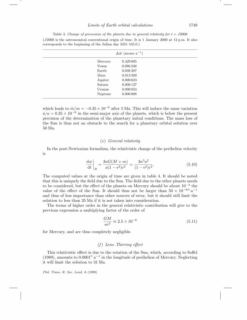
Table 4. Change of precession of the planets due to general relativity for t = J2000

(J2000 is the astronomical conventional origin of time. It is 1 January 2000 at 12 p.m. It alsocorresponds to the beginning of the Julian day 2451 545.0.)

∆$ (arcsec a−1)

Mercury 0.429 805Venus 0.086 246Earth 0.038 387Mars 0.013 509Jupiter 0.000 623Saturn 0.000 137Uranus 0.000 024Neptune 0.000 008

which leads to m/m = −0.35× 10−6 after 5 Ma. This will induce the same variationa/a = 0.35× 10−6 in the semi-major axis of the planets, which is below the presentprecision of the determination of the planetary initial conditions. The mass loss ofthe Sun is thus not an obstacle to the search for a planetary orbital solution over50 Ma.

(e) General relativity

In the post-Newtonian formalism, the relativistic change of the perihelion velocityis

d$dt

∣∣∣∣R

=3nG(M +m)a(1− e2)c2

=3n3a2

(1− e2)c2. (5.10)

The computed values at the origin of time are given in table 4. It should be notedthat this is uniquely the field due to the Sun. The field due to the other planets needsto be considered, but the effect of the planets on Mercury should be about 10−4 thevalue of the effect of the Sun. It should thus not be larger than 50 × 10−6′′ a−1

and thus of less importance than other sources of error, but it should still limit thesolution to less than 35 Ma if it is not taken into consideration.

The terms of higher order in the general relativistic contribution will give to theprevious expression a multiplying factor of the order of

GM

ac2≈ 2.5× 10−8 (5.11)

for Mercury, and are thus completely negligible.

(f ) Lens–Thirring effect

This relativistic effect is due to the rotation of the Sun, which, according to Soffel(1989), amounts to 0.0001′′ a−1 in the longitude of perihelion of Mercury. Neglectingit will limit the solution to 31 Ma.


1750 J. Laskar

Table 5. Change of precession of the planets due to the effect of a solar J2 = 2× 10−6

∆$ (arcsec a−1) ∆Ω (arcsec a−1)

Mercury 0.002 435 −0.002 435Venus 0.000 261 −0.000 261Earth 0.000 084 −0.000 084Mars 0.000 019 −0.000 019

(g) J2 of the Sun

The J2 value of the Sun is not well known (see next section), but it is supposed to besmall. Contrary to general relativity, the quadrupole moment of the Sun (J2) affectsboth the longitude of node and perihelion (this is a way to discriminate between thetwo contributions). The rate of the perihelion due to the J2 of the Sun is given by

d$dt

∣∣∣∣J2

= 34J2

(Ra

)2 5 cos2 i− 2 cos i− 1(1− e2)2 n, (5.12)

where R is the radius of the Sun, n the mean motion of the planet, and i theinclination of the planet’s orbit with respect to the equator of the Sun. The changein the rate of the node is

dΩdt

∣∣∣∣J2

= −32J2

(Ra

)2 cos i(1− e2)2n, (5.13)

which gives for the various planets the values given in table 5 for J2 = 2× 10−6. Forthis value of J2, the precession due to the J2 of the Sun is of ca. 0.003′′ a−1. Thiswould lead to an error of ca. 0.075 rad after 5 Ma, which would limit the validity ofthe solution to

TV ≈ 16 Ma. (5.14)

If the uncertainty on this term, which is the largest one considered so far, is reducedby a factor of 10 to 2×10−7, the error would be 0.01 after 5 Ma, which will still limitthe validity of the solution to

TV ≈ 26 Ma. (5.15)

(h) Uncertainty in the measurement of the J2 of the Sun

A precise measurement of the J2 of the Sun has not yet been achieved. A compi-lation of some values in the literature gives until recently very large variations of theestimated values.

Campbell & Moffat (1983) Motion of the inner planets and Icarus:

J2 = (5.5± 1.3)× 10−6. (5.16)

Landgraf (1992) Motion of Icarus:

J2 = (0.6± 5.8)× 10−6; J2 < 2× 10−5. (5.17)



Paterno et al . (1996) Measure of the flattening of the Sun:

≈ 10−7 < J2 < 5× 10−7. (5.18)

Bois & Girard (1998) Indirect measurement of the effect on the Moon’s motion,for which very accurate observations are obtained with lunar laser ranging:

J2 < 3× 10−6. (5.19)

Pijpers (1998) SOHO and GONG helioseismic data:

J2 = (2.18± 0.06)× 10−7. (5.20)

Jurgens et al . (1998) Mercury radar ranging. Value of J2 not yet determined butshould be smaller than a few 10−7.

These measurements appear to be quite different and not very conclusive, althoughthey seem to converge to a value of a few 10−7. The latest measurement of Pijpers(1998) is very precise, but it is not clear for me whether all the uncertainties of hismodel were taken into account in the computation of errors.

A direct measurement of the dynamical effect of the J2 component of the Sun isthus welcome. The measurement of Bois & Girard (1998) through the lunar laserranging data is interesting, but the intricate motion of the Moon, which is subjectedto many other perturbations, should make it more difficult than direct measurementson Mercury. In this respect, as long as a drag-free solar probe is not used, the radarmeasurements made by Jurgens et al . (1998) should be at present the most effectiveway to obtain a direct determination of the J2 of the Sun’s gravity field, and in anycase to bound its possible value.

6. First conclusions

Quite surprisingly, we have found that, at present, the main source of uncertainty forthe construction of an accurate orbital solution for the Earth is the uncertainty inthe determination of the J2 value of the Sun. Even if there is some improvement inthe near future, and if this error goes down to 10−7, the validity time of the solutionwill be limited to 26 Ma. If this error decreases to 10−8, the solution could be validover 36 Ma, but we have seen that for this time span, there are several other sourcesof uncertainty which will limit the validity of the solution. At present, I would saythat an attainable goal is to provide an accurate solution over 35 Ma. It can also besaid that the present solution La93 is certainly not valid over more than 10–20 Ma,as was stated in Laskar et al . (1993a).

7. Precession and obliquity

Once the orbital solution of the Earth is known, one can compute the solution for theevolution of the Earth’s precession and obliquity. The uncertainty resulting from thiscomputation is of a different nature. Indeed, the motion of the obliquity is essentiallystable, despite the proximity of a small resonance induced by the perturbation ofJupiter and Saturn (Laskar et al . 1993a, b). On the other hand, the rotational motionof the Earth is subject to various dissipative effects for which the amplitude andcorrect method of modelling are not known precisely (see Neron de Surgy & Laskar(1997) for a more complete review).


1752 J. Laskar

(a) Change in the dynamical ellipticity of the Earth

Although the possibility of changes in the dynamical ellipticity of the Earth wasknown for a long time, attention was drawn to it recently by Laskar et al . (1993a),when we demonstrated the proximity of the precession–obliquity solution of theEarth with a resonance with the s6−g6 +g5 term of perturbation due to Jupiter andSaturn. Although this excitation term is small, we demonstrated that it induces someimportant effects in the present solution of the obliquity of the Earth. Moreover, weshowed that a very small change in the dynamical ellipticity of the Earth, of about0.002 in relative size, could allow for a passage into resonance, thus inducing largerchanges in the obliquity. In Laskar et al . (1993a), based on calculations by Thomson(1990), we mentioned that such a small change in the dynamical ellipticity of theEarth could be obtained by passage through an ice age, because of the change in therepartition of the mass loads on the Earth.

These findings were followed by new computations yielding improved estimates forthe possible change in dynamical ellipticity when entering into an ice age (Peltier &Jiang 1994; Mitrovica & Forte 1995), which reveals the effects to be much smallerthan the previous estimate used in Laskar et al . (1993a). With these new values, thepassage into the resonance s6 − g6 + g5 could no longer be obtained during an iceage. Nevertheless, the proximity of the resonance should still have a singular effecton the obliquity solution, and it should be noted that, due to the tidal evolutionof the Earth–Moon system, we will surely enter into this resonance in the nearfuture.

Recently, Forte & Mitrovica (1997) demonstrated that mantle convection couldalso have induced some small decrease in the dynamical ellipticity in the past, on alonger time-scale, which could reach about 0.01 within 20 Ma. They argued that thiscould allow again for a passage into the small Jupiter–Saturn resonance, but this isnot clear since tidal evolution will have the opposite effect on this time-scale.

A different effect can also result from multiple passages into ice ages. Provided acertain time lag exists between the forcing of the obliquity and the ice age response(i.e. also the change in dynamical ellipticity), then a secular trend can occur in thevariation of the obliquity of the Earth (Rubincam 1990, 1995; Bills 1994; Ito etal . 1995; Williams et al . 1998). Nevertheless, these effects occur only on very longtime-scales, and their actual amplitude is still very controversial.

(b) Tidal dissipation

Due to the non-elasticity of the Earth, and to the fact that the Earth rotatesfaster on its axis than the Moon around the Earth, there will exist an offset betweenthe tidal deformation of the Earth and the Earth–Moon direction. This inducesa breaking couple on the rotation of the Earth, and by conservation of angularmomentum, a slow increase in the Earth–Moon distance.

The first understanding of the tidal evolution of the Earth–Moon system wasobtained by Darwin (1880), while modern developments are due to Kaula (1964),MacDonald (1964), Goldreich & Peale (1966), Goldreich (1966), Goldreich & Soter(1966), Lambeck (1979), Mignard (1979, 1980, 1981), Ward (1982), Laskar & Robutel(1993), Laskar et al . (1993b), Touma & Wisdom (1994) and Neron de Surgy & Laskar(1997).



The introduction of these tidal terms in the computation of the evolution of theprecession and obliquity of the Earth over several millions of years was made inQuinn et al . (1991), Laskar et al . (1993a) and Neron de Surgy & Laskar (1997),while the resulting change in insolation was discussed in Berger et al . (1989).

In the La93 solutions, it was recognized that the uncertainty left in the value ofthe tidal dissipation, as well as the possible change of dynamical ellipticity, were themajor sources of uncertainty for the precession and obliquity solution over 10–20 Ma.These two parameters were thus left free in the solutions, so that one could adjustthem in the light of geological data. This was done in particular by Lourens et al .(1996).

(c) Core–mantle interactions

Another source of dissipation occurs at the core–mantle limit, due to the differenceof the precessing rate of the core and the mantle (Rochester 1976; Goldreich & Peale1966, 1967; Greenspan & Howard 1963; Lumb & Aldridge 1991; Neron de Surgy &Laskar 1997).

The exact value of this dissipation is largely unknown, as it depends on the effectiveviscosity of the outer core, but comparisons with available geological data for theevolution of the length of the day (Neron de Surgy & Laskar 1997) allow boundariesto be set on the possible value of this dissipation, which would not very much affectthe solutions over 10–20 Ma. More precisely, since the value of the viscosity cannot bevery large, it is difficult to discern the difference between a dissipation due to core–mantle interaction, and a tidal dissipation inducing the same effect on the breakingof the Earth’s rotation (although the effects on the evolution of the obliquity aredifferent).

(d) Conclusions

The uncertainty of the dissipative effects due to tidal dissipation, core–mantleinteractions, and changes in dynamical ellipticity are real, but if the geological dataare precise enough, this should not be a real problem for the orbital solution. Indeed,the behaviour of obliquity is stable, and fitting the dissipative contribution to thegeological data should be possible, as has already been done in Lourens et al . (1996).

8. Beyond chaos

In the previous sections we have seen that in order to obtain an accurate solutionfor the orbital motion, we are practically limited to 35 Ma, due to the exponentialdivergence of the solutions. On the other hand, the dissipative effects present a largeuncertainty, but they can be adjusted in the light of the geological data. The questionwhich remains is how to cope with the chaos, or more precisely, is it possible withoutpretending to have an accurate solution for the Earth to still get some informationin an astronomical solution to use to obtain a geological time-scale over much longertimes, extending over 250 Ma, which correspond roughly to the time-scale for whichgeological data are available?

In order to address this problem, one needs to look more closely at the expectedsignal which can be extracted from the geological data.


1754 J. Laskar

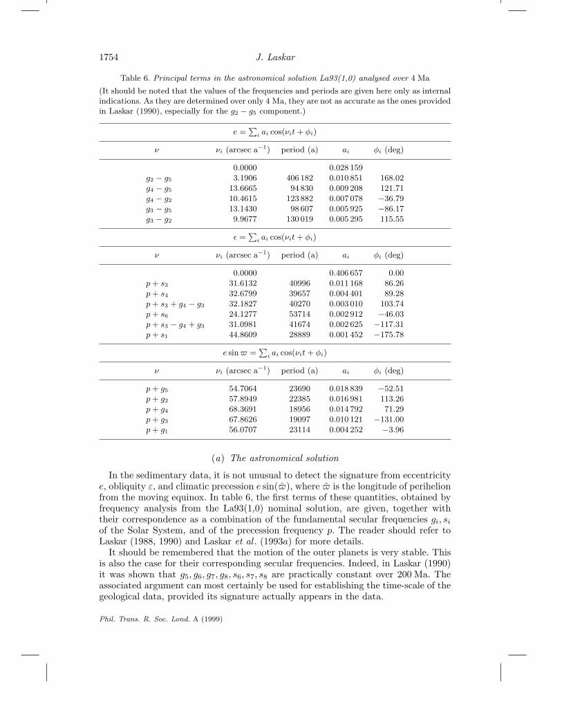
Table 6. Principal terms in the astronomical solution La93(1,0) analysed over 4 Ma

(It should be noted that the values of the frequencies and periods are given here only as internalindications. As they are determined over only 4 Ma, they are not as accurate as the ones providedin Laskar (1990), especially for the g2 − g5 component.)

e =∑i ai cos(νit+ φi)

ν νi (arcsec a−1) period (a) ai φi (deg)

0.0000 0.028 159g2 − g5 3.1906 406 182 0.010 851 168.02g4 − g5 13.6665 94 830 0.009 208 121.71g4 − g2 10.4615 123 882 0.007 078 −36.79g3 − g5 13.1430 98 607 0.005 925 −86.17g3 − g2 9.9677 130 019 0.005 295 115.55

ε =∑i ai cos(νit+ φi)


0.0000 0.406 657 0.00p+ s3 31.6132 40996 0.011 168 86.26p+ s4 32.6799 39657 0.004 401 89.28p+ s3 + g4 − g3 32.1827 40270 0.003 010 103.74p+ s6 24.1277 53714 0.002 912 −46.03p+ s3 − g4 + g3 31.0981 41674 0.002 625 −117.31p+ s1 44.8609 28889 0.001 452 −175.78

e sin$ =∑i ai cos(νit+ φi)


p+ g5 54.7064 23690 0.018 839 −52.51p+ g2 57.8949 22385 0.016 981 113.26p+ g4 68.3691 18956 0.014 792 71.29p+ g3 67.8626 19097 0.010 121 −131.00p+ g1 56.0707 23114 0.004 252 −3.96

(a) The astronomical solution

In the sedimentary data, it is not unusual to detect the signature from eccentricitye, obliquity ε, and climatic precession e sin($), where $ is the longitude of perihelionfrom the moving equinox. In table 6, the first terms of these quantities, obtained byfrequency analysis from the La93(1,0) nominal solution, are given, together withtheir correspondence as a combination of the fundamental secular frequencies gi, siof the Solar System, and of the precession frequency p. The reader should refer toLaskar (1988, 1990) and Laskar et al . (1993a) for more details.

It should be remembered that the motion of the outer planets is very stable. Thisis also the case for their corresponding secular frequencies. Indeed, in Laskar (1990)it was shown that g5, g6, g7, g8, s6, s7, s8 are practically constant over 200 Ma. Theassociated argument can most certainly be used for establishing the time-scale of thegeological data, provided its signature actually appears in the data.



2

0

π

2π

4π

6π

8–200– 150– 100– 50 50 100

time (Ma)

2( (4

.4

.– – –) )ϖ 3

.3

.ϖ Ω Ω

150 2000–

–

–

–

π

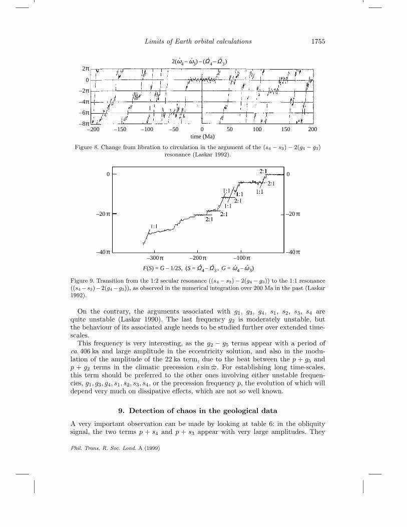
Figure 8. Change from libration to circulation in the argument of the (s4 − s3)− 2(g4 − g3)resonance (Laskar 1992).

0

20 π

40ππ300– π200– π100–

–

–

0

20 π

40π–

–

4 3(S = F(S) = G – 1/2S,.

– ),.

ϖ ϖΩ Ω 4 3G = .

–.

Figure 9. Transition from the 1:2 secular resonance ((s4 − s3)− 2(g4 − g3)) to the 1:1 resonance((s4−s3)−2(g4−g3)), as observed in the numerical integration over 200 Ma in the past (Laskar1992).

On the contrary, the arguments associated with g1, g3, g4, s1, s2, s3, s4 arequite unstable (Laskar 1990). The last frequency g2 is moderately unstable, butthe behaviour of its associated angle needs to be studied further over extended time-scales.

This frequency is very interesting, as the g2 − g5 terms appear with a period ofca. 406 ka and large amplitude in the eccentricity solution, and also in the modu-lation of the amplitude of the 22 ka term, due to the beat between the p + g5 andp + g2 terms in the climatic precession e sin $. For establishing long time-scales,this term should be preferred to the other ones involving either unstable frequen-cies, g1, g3, g4, s1, s2, s3, s4, or the precession frequency p, the evolution of which willdepend very much on dissipative effects, which are not so well known.

9. Detection of chaos in the geological data

A very important observation can be made by looking at table 6: in the obliquitysignal, the two terms p + s4 and p + s3 appear with very large amplitudes. They


1756 J. Laskar

will thus induce a modulation in the amplitude of the 40 ka signal, with frequencyof s3 − s4 ≈ 1.0667′′ a−1 (period ca. 1.215 Ma). Such a signal seems to be present inthe ODP 154 record (see Shackleton et al ., this issue).

On the other hand, in the climatic precession, the two terms p+g4 and p+g3 shouldinduce also a modulation of frequency g4−g3 ≈ 0.5236′′ a−1 (period ca. 2.475 Ma) inthe 19 ka term of the climatic precession, as well as in the 95 and 125 ka terms in theeccentricity. For these two last terms, it should be noted that even if the resolution ofthe data does not make it possible to discriminate between the 95 and 125 ka terms,the modulation of the amplitude of these terms is the same, and thus could still bediscernible in the geological record.

If it were possible to obtain these two modulations from the geological data, thiswould have important consequences. Indeed, in Laskar (1990) it was demonstratedthat the resonance

(s4 − s3)− 2(g4 − g3) = 0 (9.1)

is one of the main sources of the chaotic behaviour in the motion of the planets.Moreover, I could show that presently we are in a librational state with respect tothis resonance, but this can evolve in a rotational state, and even slowly move tolibration in a new resonance, namely

(s4 − s3)− (g4 − g3) = 0. (9.2)

The transition from this 1:2 resonance of s4 − s3 and g4 − g3 to the 1:1 resonanceshould be possible to detect. If this is the case, this would be the signature of thechaotic motion of the planets. Moreover, the dating, even in a very approximatemanner of these transitions, would provide very precise constraints on the dynamicalmodel for the evolution of the Solar System. It would be even more important to findthe first transition in the past, as this would be the event which could be actuallyused for adjusting (or at least testing) the parameters of the orbital solution. Oneshould realize that in this case the exponential divergence of the solution will be usedin the reverse way to that in which it was used in the first sections of this paper, andcould make it possible to obtain very precise information on the initial conditionsand (or) parameters of the model. One could even dream that if the succession of thetransitions from the 1:2 to the 1:1 resonance were found and dated over an intervalof 200 Ma that this could be the ultimate test for the gravitational model. It wouldmake it possible, for example, to obtain the J2 value of the Sun with high accuracy,or to test the model of general relativity.

10. Conclusion

Due to the chaotic behaviour, the time of validity for a precise orbital solutionof the Earth will be in practice limited to 35–50 Ma. Moreover, one of the mainsources of uncertainty at present is the imprecision in the measurement of the J2value of the Sun which could even bring this limit down to a much shorter timespan. Nevertheless, it can be forecast that within five years much more accurateknowledge of this quantity should be obtained. In this case, there are still numeroussources of uncertainty which will limit the solution to 35–50 Ma.

There are also several sources of uncertainty for the dissipative effects in the evo-lution of the rotational and precession motion of the Earth, but comparison with



the geological data should permit adjustment of these quantities. It should also bepossible to use the astronomical time-scale beyond the limit of 35–50 Ma if oneacknowledges the unavailability of an accurate solution for the orbital motion of theEarth, but searches in the data for the signature of frequencies related to the motionof the outer planets, which is predictable over much longer time-scales.

Moreover, the s4−s3 and g4−g3 frequencies induce some modulation in the ampli-tude of the obliquity and eccentricity or climatic precession. It should thus be possibleto observe in the geological data the trace of transition from the (s4−s3)−2(g4−g3)secular resonance to the (s4 − s3) − (g4 − g3) resonance. The detection and datingof these passages, which are the signature of the chaotic behaviour of the planets,should induce extremely high constraints on the dynamical models for the orbitalevolution of the Solar System. This gives a unique and challenging opportunity forpalaeoclimate records to provide some of the ultimate constraints on the dynamicalmodels for the evolution of the Solar System.

Many discussions with colleagues have been very helpful in the preparation of this paper. Theauthor is particularly grateful to L. Blanchet, E. Bois, A. Correia, N. Shackleton, M. Sladeand E. M. Standish for discussions. The integration of the Earth–Moon system was performedby R. Michelsen in his Master’s thesis, and technical help was given by M. Gastineau. Thecomputations were performed at CNUSC–CNRS, and this work benefited from the help of theCEE contract CHRX-CT94-0460.

References

Berger, A. 1976 Obliquity and precession for the last 5,000,000 years. Astron. Astrophys. 51,127–135.

Berger, A. 1978 Long-term variations of daily insolation and quaternary climatic changes. J.Atmos. Sci. 35, 2362–2367.

Berger, A., Loutre, M. F. & Dehant, V. 1989 Influence of the changing lunar orbit on theastronomical frequencies of pre-quaternary insolation patterns. Paleoceanography 4, 555–564.

Bills, B. G. 1994 Obliquity–oblateness feedback: are climatically sensitive values of obliquitydynamically unstable? Geophys. Res. Lett. 21, 177–180.

Bois, E. & Girard, J. F. 1998 Impact of the quadrupole moment of the Sun on the dynamics ofthe Earth–Moon system. Preprint.

Bretagnon, P. 1974 Termes a longue periodes dans le systeme solaire. Astron. Astrophys. 30,141–154.

Bretagnon, P. 1984 Amelioration des theories planetaires analytiques. Celest. Mech. 34, 193–201.Brouwer, D. & Van Woerkom, A. J. J. 1950 The secular variations of the orbital elements of the

principal planets. Astron. Papers Am. Ephem. 13(II), 81–107.Campbell, L. & Moffat, J. W. 1983 Quadrupole moment of the Sun and the planetary orbits.

Astrophys. J. 275, L77–L79.Darwin, G. H. 1880 On the secular change in the elements of a satellite revolving around a

tidally distorted planet. Phil. Trans. R. Soc. Lond. 171, 713–891.Dickey, J. O. (and 11 others) 1994 Lunar laser ranging: a continuating legacy of the Apollo

program. Science 265, 182–190.Forte, A. & Mitrovica, J. X. 1997 A resonance in the Earth’s obliquity and precession over the

past 20 Myr driven by mantle convection. Nature 390, 676–680.Goldreich, P. 1966 History of the lunar orbit. Rev. Geophys. 4, 411–439.Goldreich, P. & Peale, S. 1966 Spin orbit coupling in the Solar System. Astron. J. 71, 425–438.Goldreich, P. & Peale, S. 1967 Spin-orbit coupling in the Solar System. II. The resonant rotation

of Venus. Astron. J. 72, 662–668.


1758 J. Laskar

Goldreich, P. & Soter, S. 1966 Q in the Solar System. Icarus 5, 375–389.Greenspan, H. P. & Howard, L. N. 1963 J. Fluid Mech. 17, 385.Hill, G. 1897 On the values of the eccentricities and longitudes of the perihelia of Jupiter and

Saturn for distant epochs. Astron. J. 17(11), 81–87.Ito, T., Masuda, K., Hamano, Y. & Matsui, T. 1995 Climate friction: a possible cause for secular

drift of Earth’s obliquity. J. Geophys. Res. 100, 15 147–15 161.Jurgens, R. F., Rojas, F., Slade, M. A. & Standish, E. M. 1998 Mercury radar ranging data

from 1987 to 1997. Astron. J. 116, 486–488.Kaula, W. 1964 Tidal disipation by solid friction and the resulting orbital evolution. J. Geophys.

Res. 2, 661–685.Lambeck, K. 1979 On the orbital evolution of the Martian satellites. J. Geophys. Res. B 84,

5651–5658.Lambeck, K. 1980 The Earth’s variable rotation. Cambridge University Press.Landgraf, W. 1992 An estimation of the oblateness of Sun from the motion of Icarus. Solar

Physics 142, 403–406.Laskar, J. 1984 Theorie generale planetaire: elements orbitaux des planetes sur 1 million

d’annees. These, Observatoire de Paris, France.Laskar, J. 1985 Accurate methods in general planetary theory. Astron. Astrophys. 144, 133–146.Laskar, J. 1986 Secular terms of classical planetary theories using the results of general theory.

Astron. Astrophys. 157, 59–70.Laskar, J. 1988 Secular evolution of the Solar System over 10 million years. Astron. Astrophys.

198, 341–362.Laskar, J. 1989 A numerical experiment on the chaotic behaviour of the Solar System. Nature

338, 237–238.Laskar, J. 1990 The chaotic motion of the Solar System: a numerical estimate of the size of the

chaotic zones. Icarus 88, 266–291.Laskar, J. 1992 A few points on the stability of the Solar System. In Chaos, resonance and

collective dynamical phenomena in the Solar System (ed. S. Ferraz-Mello), pp. 1–16. IAUSymposium 152. Kluwer.

Laskar, J. & Robutel, P. 1993 The chaotic obliquities of the planets. Nature 361, 608–612.Laskar, J., Joutel, F. & Boudin, F. 1993a Orbital, precessional, and insolation quantities for the

Earth from −20 Myr to +10 Myr. Astron. Astrophys. 270, 522–533.Laskar, J., Joutel, F. & Robutel, P. 1993b Stabilization of the Earth’s obliquity by the Moon.

Nature 361, 615–617.Le Verrier, U. 1856 Ann. Obs. Paris, vol. II. Paris: Mallet-Bachelet.Le Verrier, U. 1858 Ann. Obs. Paris, vol. IV. Paris: Mallet-Bachelet.Lourens, L. J., Hilgen, F. J., Zachariasse, W. J., Van Hoof, A. A. M., Antonarakou, A. &

Vergnaud-Grazzini, C. 1996 Evaluation of the Plio-Pleistocene astronomical time scale. Pale-oceanography 11, 391–413.

Lumb, L. I. & Aldridge, K. D. 1991 On viscosity estimates for the Earth’s fluid outer core andcore–mantle coupling. J. Geomagn. Geoelectr. 43, 93–110.

MacDonald, G. J. F. 1964 Tidal friction. J. Geophys. Res. 2, 467–541.Mignard, F. 1979 The evolution of the lunar orbit revisited. I. Moon Planets 20, 301–315.Mignard, F. 1980 The evolution of the lunar orbit revisited. II. Moon Planets 23, 185–206.Mignard, F. 1981 The evolution of the lunar orbit revisited. III. Moon Planets 24, 189–207.Mitrovica, J. X. & Forte, A. 1995 Pleistocene glaciation and the Earth’s precession constant.

Geophys. J. Int. 121, 21–32.Neron de Surgy, O. & Laskar, J. 1997 On the long term evolution of the spin of the Earth.

Astron. Astrophys. 318, 975–989.



Paterno, L., Sofia, S. & DiMauro, M. P. 1996 The rotation of the Sun’s core. Astron. Astrophys.314, 940–946.

Peltier, W. R. & Jiang, X. 1994 Precession constant of the Earth: variations through the ice-age.Geophys. Res. Lett. 21, 2299–2302.

Pijpers, F. P. 1998 Helioseismic determination of the solar gravitational quadrupole moment.Mon. Notes R. Astr. Soc. 297, L76–L80.

Quinn, T. R., Tremaine, S. & Duncan, M. 1991 A three million year integration of the Earth’sorbit. Astron. J. 101, 2287–2305.

Rochester, M. G. 1976 The secular decrease of obliquity due to dissipative core–mantle coupling.Geophys. J. R. Astr. Soc. 46, 109–126.

Rubincam, D. P. 1990 Mars: change in axial tilt due to climate? Science 248, 720–721.Rubincam, D. P. 1995 Has climate changed Earth’s tilt? Paleoceanography 10, 365–372.Sharav, S. G. & Boudnikova, N. A. 1967a On secular perturbations in the elements of the Earth’s

orbit and their influence on the climates in the geological past. Bull. ITA 11, 231–265.Sharav, S. G. & Boudnikova, N. A. 1967b Secular perturbations in the elements of the Earth’s

orbit and the astronomical theory of climate variations. Trud. ITA 14, 48–84.Soffel, M. H. 1989 Relativity in astrometry, celestial mechanics and geodesy. Springer.Standish, E. M. 1998 JPL planetary and lunar ephemerides. DE405/LE405, JPL-IOM, 312F-

98-048.Thomson, D. J. 1990 Quadratic-inverse spectrum estimates: applications to palaeoclimatology.

Phil. Trans. R. Soc. Lond. A 332, 539–597.Touma, J. & Wisdom, J. 1994 Evolution of the Earth–Moon system. Astron. J. 108, 1943–1961.Ward, W. R. 1982 Comments on the long-term stability of the Earth’s obliquity. Icarus 50,

444–448.Williams, D. M., Kasting, J. F. & Frakes, L. A. 1998 Low-latitude glaciation and rapid changes

in the Earth’s obliquity explained by obliquity–oblateness feedback. Nature 396, 453–455.


the limits of earth orbital calculations for geological time-scale use

Documents