EDHEC-Risk Institute393-400 promenade des Anglais06202 Nice Cedex 3Tel.: +33 (0)4 93 18 32 53

E-mail: research@edhec-risk.comWeb: www.edhec-risk.com

The Link between Eurozone Sovereign Debt and CDS Prices

January 2012

Dominic O’Kane,Affiliated Professor of Finance, EDHEC Business School

2

AbstractWe perform a theoretical and empirical analysis of the relationship between the price of Eurozone sovereign-linked credit default swaps (CDS) and the same sovereign bond markets during the Eurozone debt crisis of 2009-2011. We first present a simple model which establishes the no-arbitrage relationship between CDS and bond yield spreads. We then test this relationship empirically and explain why the market may deviate from it. Reasons include the different currencies of denomination of market-standard CDS and their reference obligations. We also examine whether CDS spread cause changes in bond spreads, and vice-versa, in a Granger sense. We find evidence for a Granger causal relationship with a one day lag from CDS to bonds for Greece and Spain, the reverse relationship for France and Italy and a feedback relationship for Ireland and Portugal.

The author thanks Douglas Keenan, Sergio Focardi, Joelle Miffre and Lutz Schloegl for helpful comments.

EDHEC is one of the top five business schools in France. Its reputation is built on the high quality of its faculty and the privileged relationship with professionals that the school has cultivated since its establishment in 1906. EDHEC Business School has decided to draw on its extensive knowledge of the professional environment and has therefore focused its research on themes that satisfy the needs of professionals.

EDHEC pursues an active research policy in the field of finance. EDHEC-Risk Institute carries out numerous research programmes in the areas of asset allocation and risk management in both the traditional and alternative investment universes. Copyright © 2012 EDHEC

IntroductionThere is a theoretical no-arbitrage relationship between the prices of credit default swap (CDS) contracts on a reference entity and the credit spreads of same currency par bonds issued by the same reference entity. In practice this relationship is held approximately and deviations may appear for either fundamental or market reasons. Fundamental reasons are those due to the exact mechanics of a bond and CDS which mean that a bond plus CDS position is not a perfect credit hedge. Market reasons relate to factors such as liquidity, and supply and demand. These factors are set out in detail in O’Kane & McAdie (2001).

More recently, policy makers have started1 to move against the use of naked CDS suggesting that the speculative use of CDS by market participants has caused or accelerated the rapid decline in 2010-11 of the bond prices of the eurozone periphery countries of Portugal, Ireland, Italy, Greece and Spain, hereafter known by the acronym PIIGS. The aim of this paper is to quantify and empirically test the relationship between the CDS and bond markets and to see if any such causation can be detected. However, pure causation in a physical sense is hard to prove from time series data alone since a transmission mechanism needs to be demonstrated. Such a mechanism may or may not exist and if it does exist, it may not be easily observed. We can however test for weaker forms of causality such as Granger causality (Baltagi, 2011). This establishes whether or not there is a measure of predictive causality between two variables X and Y in the sense that past values of Y improve our ability to predict future values of X more than with just past values of X. If this is the case, then we say that Y Granger causes X. We can also test the reverse hypothesis that X Granger causes Y.

Previous work by Das (2011) suggests that the greater convenience of the CDS market means that price discovery occurs there before it does in the bond market. Work by Levy (2009) shows that there is little empirical support for the idea that CDS markets lead bond markets. Levy finds that decreases in CDS liquidity causes the CDS spread to increase while counterparty risk causes CDS spreads to decrease. A more recent paper by Calice, Chen and Williams (2011) has examined the effect of liquidity spillovers between the CDS and government bond markets and determined that the liquidity of the CDS market has a substantial influence on sovereign debt spreads.2 There are fundamental differences between the sovereign-linked CDS and bond markets. The CDS market is an OTC market dealing with synthetic assets while the bond market trades a range of physical bonds each with a specific maturity, coupon and outstanding liquidity. The bond market is usually more liquid for bond buyers than it is for short sellers due to the need to source a physical asset to reverse repo. The CDS market is equally liquid in both directions. This makes the CDS the preferred instrument for those seeking to implement a short credit position. The CDS market also makes it is easier to trade in large size with most trades occurring in multiples of $10m.

The CDS market also makes it easier to leverage, although this is less true than before as the introduction of fixed coupons in 2009 means that there will usually be a significant upfront cost even before the reference credit becomes severely distressed, i.e. trading above approximately 1000bp in par CDS spread terms. Although they differ in format, CDS and bonds essentially trade the same underlying credit risk. At a micro market-structure level, we also note that most dealers have the same trader making markets in both the CDS and bonds. We would therefore expect that the arrival of new information about the reference entity sovereign, plus relative market demand for one format versus the other will quickly be reflected in the prices of both.

3

1 - http://www.ft.com/intl/cms/s/0/cc9c5050-f96f-11e0-bf8f-00144feab49a.html#axzz1fggjlgPA2 - We do not address the question of relative liquidity in this paper other than to note that our initial studies of bond and CDS bid-ask spreads (not presented in this paper) show that in times of crisis the bond market become less liquid while the CDS market’s liquidity remains more robust. In certain countries the CDS market can become more liquid than the bond market.

4

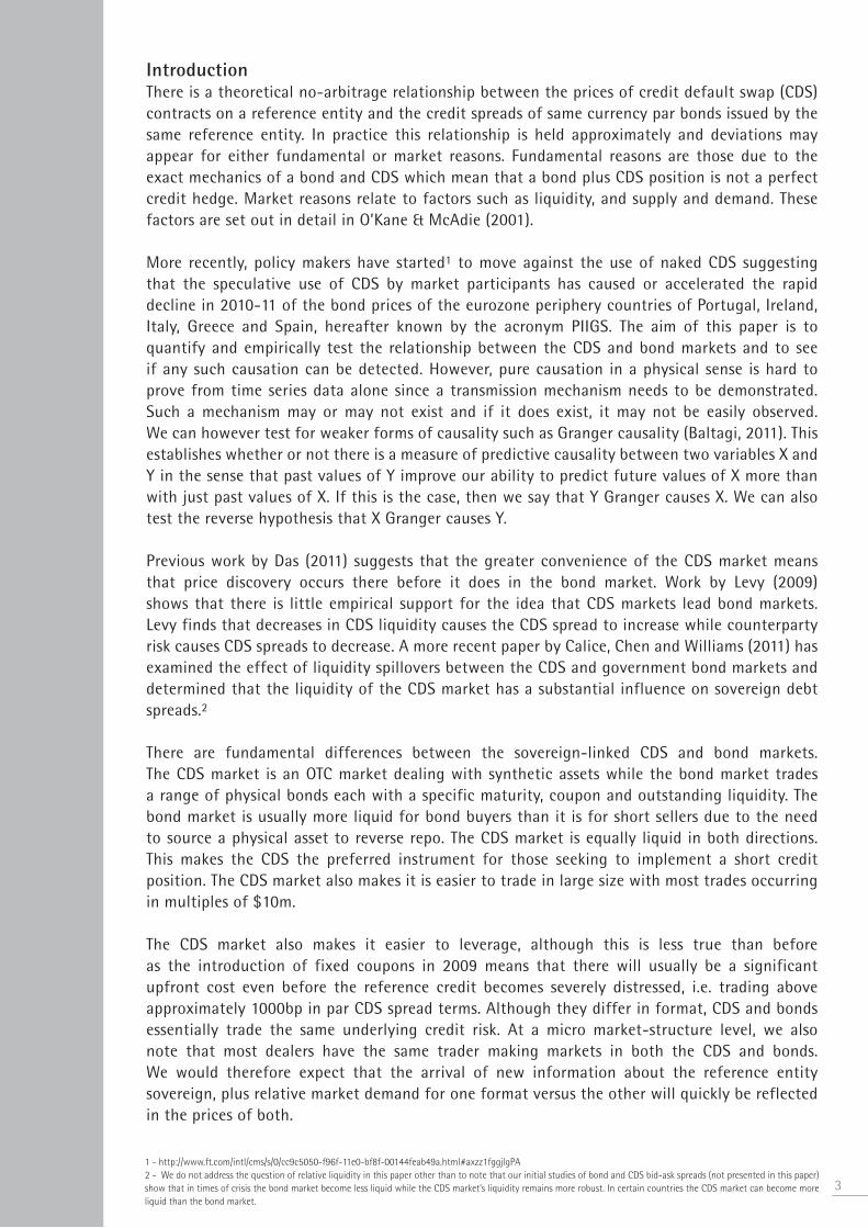
Although the CDS market may be more nimble than the bond market for short sellers, it must also be noted that it is also much smaller, especially when measured on a net risk basis, i.e. once all contracts within each legal entity have been netted3. Figure 1 shows a comparison of the percentage of the total external debt for each sovereign that its CDS represent. These numbers are taken from the DTCC4, a NY-based trade repository which contains more than 97% of all CDS transactions. We see that while the gross notional of CDS for Greece and Italy are about 14% of their total external debt, the net notional of CDS is much smaller at around 1%. Both the gross and net notionals are even smaller percentages of the total external debt for the other countries. Figure 1: CDS gross and net notional market size as a percentage of total external debt. The CDS numbers are from the DTCC as of September 2011 while the debt numbers are from June 2010.

The dynamics of the relationship between bonds and CDS also reflects the different types of market participants who buy protection. There are bank loan and bond book managers who buy protection to hedge existing bonds and loans as an alternative to selling them.5 There are also trading desks buying protection in order to hedge their credit value adjustment (CVA) risk.6 There are also those who buy protection either in the process of implementing a negative basis strategy7 or unwinding a positive basis strategy. Finally, there are the actions of speculators, usually in hedge funds, who become outright protection buyers in the expectation that spreads will widen further and that they will be able to unwind the position later at a profit.

The structure of this paper is as follows. In the next section we set out the no-arbitrage arguments for the theoretical basis for the link between the price of CDS contracts and physical obligations on the same reference entity, and we propose a simple model to establish a link between their two different quoted spreads. We then examine reasons why this model-implied relationship can break down in practice. Following this, we perform a time series analysis of the actual CDS and bond spreads for the PIIGS and France. We look for co-integration between the CDS and bond spreads and then examine whether Granger causality is present. We then present our conclusions.

3 - Net exposure is the total notional of all contracts that will need to be settled between different legal entities following a credit event. It therefore nets all of the offsetting contracts within each counterparty. Gross exposure sums the notional of every outstanding contract. 4 - Their website is www.dtcc.com.5 - Those holding sovereign bonds using “available-for-sale” accounting treatment can use CDS to hedge both the price risk and default risk of the bond. Some holders of sovereign bonds account for them as “held-to-maturity” securities and would not be realising the price changes. They would only be using CDS to hedge the loss of principal. 6 - Managing CVA risk is the management of counterparty credit risk. 7 - A negative basis strategy is a purchase of a bond and CDS protection against it. A positive basis strategy is the short sale of a bond and a sale of CDS protection against it.

1. The Link between Bonds and CDSIt has been shown [Duffie 1999] that subject to some assumptions , a long position in a par priced floating rate note plus the purchase of the same face value of CDS protection, assuming this has zero initial cost, creates a combined position which has no credit risk in the event of default. This is because the principal loss on the par bond is exactly matched by the payment from the CDS. Avoidance of arbitrage then implies that the (annualised) spread over Libor paid by the bond should equal the (annualised) spread paid by the protection buyer on the CDS. A link is therefore established between bond and CDS pricing.

In practice, many sovereign debt buyers prefer to reduce their interest rate risk by buying the bond in an asset swap package. As a result, the main Libor-based bond spread quoted is the asset swap spread. However, as with a par floating rate note, an asset swap plus a long protection CDS position on the bond’s notional amount is not a risk-free position even if the bond is trading at par. This is because asset swaps embed an interest rate swap whose unwind value following a credit event can result in a gain or loss to the asset swap buyer.

Another strategy is to buy a par valued fixed coupon bond plus the same notional of protection. This will be hedged on the principal if there is a sudden default making the position almost exactly risk-free. In this case we can think of the bond credit spread measure as the yield-to-maturity of the bond minus the yield-to-maturity of the same maturity risk-free government bond. We will later choose to use the German yield curve as our proxy for the risk-free rate.

What these no-arbitrage strategies have in common is that they only work if the bond is initially priced at par. When the price of a bond is trading away from par, these simple strategies are no longer hedged against principal losses. If the bond is priced above par, the amount of protection bought needs to be scaled up to account for the larger loss in the event of a default. If the bond is priced below par then the amount of protection needs to be scaled down. However both strategies then require an estimate of the future recovery rate in the event of default. So although there may be a link between the CDS spread and the bond’s spread, the value of the basis strategy is no longer even an approximately perfect static hedge of the principal.

Moreover, we need to take into account that CDS now trade with a fixed coupon and an upfront payment. For highly distressed credits with a low fixed coupon, most of the cost of protection will be paid upfront. The cost of the bond plus the protection will mean that the strategy will usually cost more than par. The investor will therefore lose money if default occurs immediately. A trade scenario analysis will show that it will only be after some breakeven time that the occurrence of a credit event will cause the investor to make money since time is needed to allow the investor to receive the bond coupons. As a result, the no-arbitrage linkage between the CDS spread and the bond yield spread weakens when the bond is trading away from par as it requires investors to assume recovery rate risk and credit event timing risk. Basis traders who see a mispricing between CDS and bond spreads will only act if the reward is commensurate with the risk. This means that any mispricing, even if it violates the theoretical relationship established by a model, will persist until it becomes large enough to look attractive on a risk-return basis.

There is another CDS contractual detail which causes a basis. CDS contracts on eurozone sovereigns are denominated in dollars while the bonds which they hedge are almost always denominated in euros. Therefore, at initiation a euro-based protection buyer will usually buy a dollar denominated CDS on the face value of bonds at the initial exchange rate. In the event of a default, the loss compensation amount paid out on the protection leg10 is calculated on the dollar face value. A euro-based hedger will convert this back to euros. If a credit event on

5

8 - We assume existence of the par floating rate note to the CDS maturity, that the funding rate of the protection buyer is Libor, that the funding can be repaid at par at the time of a default, that the delivery option has no value and we ignore the impact of the lost bond coupon which is not protected by the CDS. We also assume that bond and CDS are denominated in the same currency. 9 - This depends on the Libor term structure at the time of default.10 - This is par minus the recovery rate times the contract notional. The recovery rate is the fraction of par recovered on the deliverable obligations and is determined via an auction process overseen by the ISDA

6

a eurozone sovereign occurs, we might expect that the euro will weaken against the US dollar and this will result in a windfall profit for the euro-based hedger. To prevent investors from buying protection in dollars and selling protection in euro and making money following a credit event, the dollar-denominated spread adjusts until it embeds the market view on the expected exchange rate conditional on a credit event. If the market sees devaluation as being likely then this will cause dollar denominated CDS spreads to trade at higher levels than the (non-standard and less liquid) euro-denominated equivalent.

2. Model of Implied SpreadsWe wish to establish a direct relationship between the asset swap spread, yield spread and CDS spread. In the appendix we derive a standard hazard rate model for the pricing of a credit risky bond with N remaining full coupon periods, an annual coupon c paid. We assume that a recovery R is paid at the time of default and that coupons have zero recovery. We find that the price of this bond is given by

where Q(O,t) is the risk-neutral survival probability of the reference credit to time t and Z(O,t) is the default-free discount factor. Based on this simple model we can write the different credit spreads.

Asset Swap Spread: We substitute the model bond price into the equation for the asset swap spread [O’Kane 2008] to give where the denominator is the present-value of 1 basis point paid on the floating leg of the interest rate swap, is the year fraction between successive payments in the basis convention for the floating leg of the asset swap, and

is the full price of a Libor quality version of the same bond discounted on the Libor curve as represented by the Libor discount factor .

The bond-yield spread: This is simply calculated from this model by solving for the yield-to-maturity for the credit risky bond using equation (1) and for the risk-free bond and subtracting.

The CDS spread: The CDS spread can be written in terms of the risk-free discount factors and the survival curve as follows

where we assume that this CDS is quoted in the same base currency as the reference credit.

In the case where the reference credit is denominated in a different currency from the CDS contract, we need to take into account the fact that conditional on a credit event, there may be a change in the exchange rate between the two currencies. Supposing that the reference

11 - The (assumed flat) default rate is linked to the survival probability via . 12 - Note that in order to obtain this close agreement between CDS and yield-spread, we had to set the payment frequency of the bond equal to that of the CDS for which the standard is quarterly.

7

credit is denominated in euros while the CDS contract is denominated in dollars, a simple model which incorporates such a currency effect gives where

is the ratio of the initial Eurodollar FX rate to the market expected Eurodollar FX rate at the time τ of a credit event on the sovereign. The FX rate is quoted in units of number of dollars per euro. This means that if the market expects a devaluation of the euro following a credit event, the value of k will be greater than 1 and the dollar denominated CDS should trade at a higher value than the equivalent euro denominated CDS.

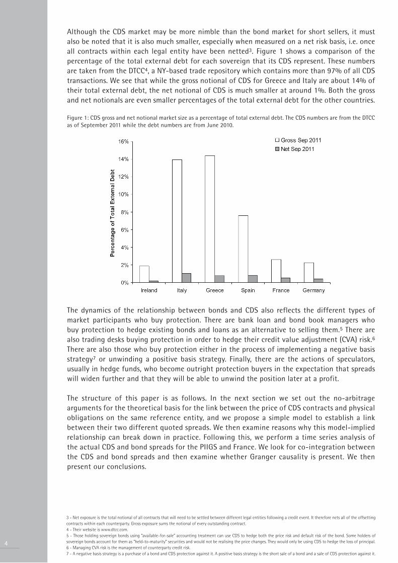
To examine the difference between these spread measures, we priced a 5-year bond with a 5% coupon in an environment where the default-free yield curve is assumed flat at 3% and the Libor risk-free curve is also assumed to be flat at 3.5%. We considered two cases - first an expected recovery rate of 40% and second an expected recovery of 0%. We then varied the 5-year survival probability assuming a flat term structure of default rates11 and calculated the implied bond price and spread measures. In all cases we assumed k = 1.

Figure 2 Comparison of the model-implied CDS, bond yield-spread and par asset swap spread measures as a function of the full price of a 5-year bond with a 6% coupon. We show this for an expected recovery of 40% (above) and 0% (below).

The results are presented in Figure 2. When the expected recovery rate is 40% we find that as the bond price falls (and it cannot fall below 40), the CDS spread grows and asymptotically tends to infinity while the yield-spread and asset swap spread tend to different large but finite numbers. However, if we set the expected recovery rate to zero then the yield-spread also tends to infinity and is very close in value to the CDS spread12 as the bond price falls to zero.

3. Choice of SpreadAlthough neither the asset swap spread nor the bond yield spread is close to the CDS spread when the bond trades away from par and the expected recovery rate is non-zero, we need to choose one or other for our empirical analysis of the relationship between bonds and CDS. We choose the bond yield. Our main reason for not choosing the asset swap spread is that it is a measure of credit quality versus Libor. As Libor is the reference rate for inter-bank lending, it embeds a compensation for the credit quality of the commercial banking sector. This means that sovereigns deemed to have a better credit quality than the banking sector will trade with a negative asset

7

8

swap spread; however the comparable CDS spread is always floored at zero. Also, movements in the asset swap spread of a sovereign debt are not purely reflective of the sovereign’s credit risk but of its credit risk relative to the banking sector. An increase in both would therefore be cancelled to some extent by a Libor-based spread measure.

Our second choice is to use the yield-spread of the bond, measured as the yield of the bond minus that of the same maturity risk-free bond, for which we choose German bonds. The advantage of the yield-spread is that it is a measure of credit risk relative to the high credit quality German yield. The size of the German bond market also means that there is only a small liquidity premium. The yield-spread is therefore almost always positive.13 To get a sense of the difference in perceived credit quality between Libor and the German yield we note that the swap spread – the 5-year Libor swap rate minus the yield on a 5-year German government bond – averaged 51bps14 and varied between 14bps and 106bps over the period January 2008 to September 2011.

4. Data DescriptionOur analysis focuses on the periphery group of Eurozone countries which have been impacted by their high levels of debt and low levels of growth. Now infamously knows as the PIIGS, these are Portugal, Ireland, Italy, Greece and Spain. We also include France in our dataset as a reference. Germany is also included. However because we have chosen to use the German yield as the effective risk-free rate in calculating the bond yield spread, we do not report any results for Germany – its yield spread is by definition zero.

Figure 3: Evolution of the 5Y CDS and Bond spreads over the sample period for Portugal, Italy, Ireland, Greece, Spain and France. Units are in basis points.

13 - The exception occurred over 6 consecutive days in January 2010 when the yield-spread of France traded as much as 5.75bp negative to Germany following the announcement of weak Q4 09 German GDP data on the 13th January 2010.14 - The average German 5-year yield was 2.55% while the average 5-year swap rate was 3.06%.

In the following we use daily close prices for CDS and bonds for the period 1 January 2008 to 1 September 2011. We focused on the 5-year maturity in both the CDS and bond markets as this is the maturity point where liquidity in the CDS market is maximal. We used Bloomberg as our CDS and bond data source. We used mid-market yield levels at the 5-year maturity over the period being analysed. These were the yields to maturities of the current on-the-run 5-year benchmark bonds in each market. Each time series contained 956 data points. Table 1 shows the main properties of both the CDS and bond yield-spread data time series. The evolution of these spreads is also shown in Figure 3.

Table 1: Descriptive statistics of the panel of CDS spread data and the bond yield-spread data used. Each data series contained 956 samples. Units are in basis points.

CDS Spread Data Bond Yield-Spread (vs. Germany)

Min Max Average Std Devn. Min Max Average Std Devn.

Portugal 14 1208 236 251 3 1497 245 314

Italy 17 388 128 73 15 412 99 66

Ireland 13 1192 275 240 10 1621 276 318

Greece 18 2477 510 541 21 2048 525 521

Spain 13 430 144 98 6 411 108 91

France 6 175 52 34 -6 74 25 13

Germany 5 91 34 19 0 0 0 0

5. Empirical AnalysisWe start by examining the relationship between the bond yield spreads and the CDS spreads. A scatter plot of the bond yield spreads versus the CDS spreads is shown in Figure 4. We have also plotted the theoretical model-implied relationship. This assumes a recovery rate of 40% and a flat term structure of spreads and interest rates. We have also set k = 1 so that no currency effect is included. We also assume a risk-free rate of 2.5%, a 3% rate for 5-year Libor, a 4% coupon on the risk-free bond and an annual 6% coupon on the risky sovereign bond.

Greece fits the theoretical curve well across the very broad range of spreads it has experienced and even presents some of the negative convexity implied by the model at high CDS spreads. In Portugal and Ireland the relationship is obeyed quite well up to about CDS spreads of 600bp. Beyond this spread level, it seems as though there is then a regime shift which causes the bonds to fall in price relative to the CDS by more than the model would imply. This could be because the bond market begins to become less liquid and this loss of liquidity causes bond prices to fall relative to CDS which continue to trade as before. It might also be because more information becomes available in the distressed prices of the bonds which cause market participants to revise downward the market-wide assumed expected recovery rate. This would increase the slope of the theoretical model. However, even with a recovery of 0%, we were unable to match the high positive slope of the relationship. Another explanation is that the market believes that a credit event may lead to the ejection of that economically weak periphery country from the eurozone resulting in a strengthening of the euro. This would be captured in our model by a value of k < 1.

9

10

Figure 4: The bond yield-spread against the CDS spread for the PIIGS and France. The red line is the model-implied relationship assuming a recovery rate of 40%.

In Italy, Spain and France the CDS spreads appear too high for the bond yields compared to the model-implied relationship. This effect could be due to the 40% recovery rate assumption being too low. It could also be a “flight to safety” effect as euro-based holders of Greek, Irish or Portuguese debt switch into the larger core Eurozone countries. This demand would push down the bond yield for those countries relative to the CDS market. It could also be a currency effect causing the dollar denominated CDS spreads to be too high relative to a model curve which assumes no currency impact following a sovereign credit event. The higher CDS spreads for Italy, Spain and France could therefore be implying that market participants would expect a devaluation of the euro following the credit event of any one of these large core Eurozone countries.

6. Dynamical AnalysisWe analyse how the changes in bond yield spreads and CDS spreads are linked. We define the yield spread at time t to be given by SBond(t) = yCountry (t) — yGermany (t) where yCountry (t) is yield-to-maturity of the 5-year benchmark bond in that country and yGermany (t) is the yield-to-maturity for a 5-year benchmark German government bond. We define SCDS (t) to be the time t 5-year CDS spread linked to the same country. Our analysis is concerned with detecting causality in the changes of the CDS and bond yield-spreads. We define ∆SBond(t) = SBond(t) — SBond(t—1) and

∆SCDS(t) = SCDS(t) — SCDS(t—1) to be the daily bond yield-spread change and CDS spread change. A starting point for analysing the dynamic relationship between bonds and CDS is to look at the cross-correlation between ∆SBond(t) and ∆SCDS(t). We calculated the instantaneous pair wise correlation between the CDS and bond yield spread. This is shown in Figure 5 below – the row corresponding to a lag of zero.

We find that the relationship is quite strong with a correlation of 60% or more for all countries except France. We suspect that the low 28.3% correlation for France is due to a previously mentioned “flight to safety” effect which means that when France’s CDS spreads are widening due to the contagion from the problems of the periphery countries, bond investors are often buying French debt, viewing France and Germany as the Eurozone’s safe haven bond markets.

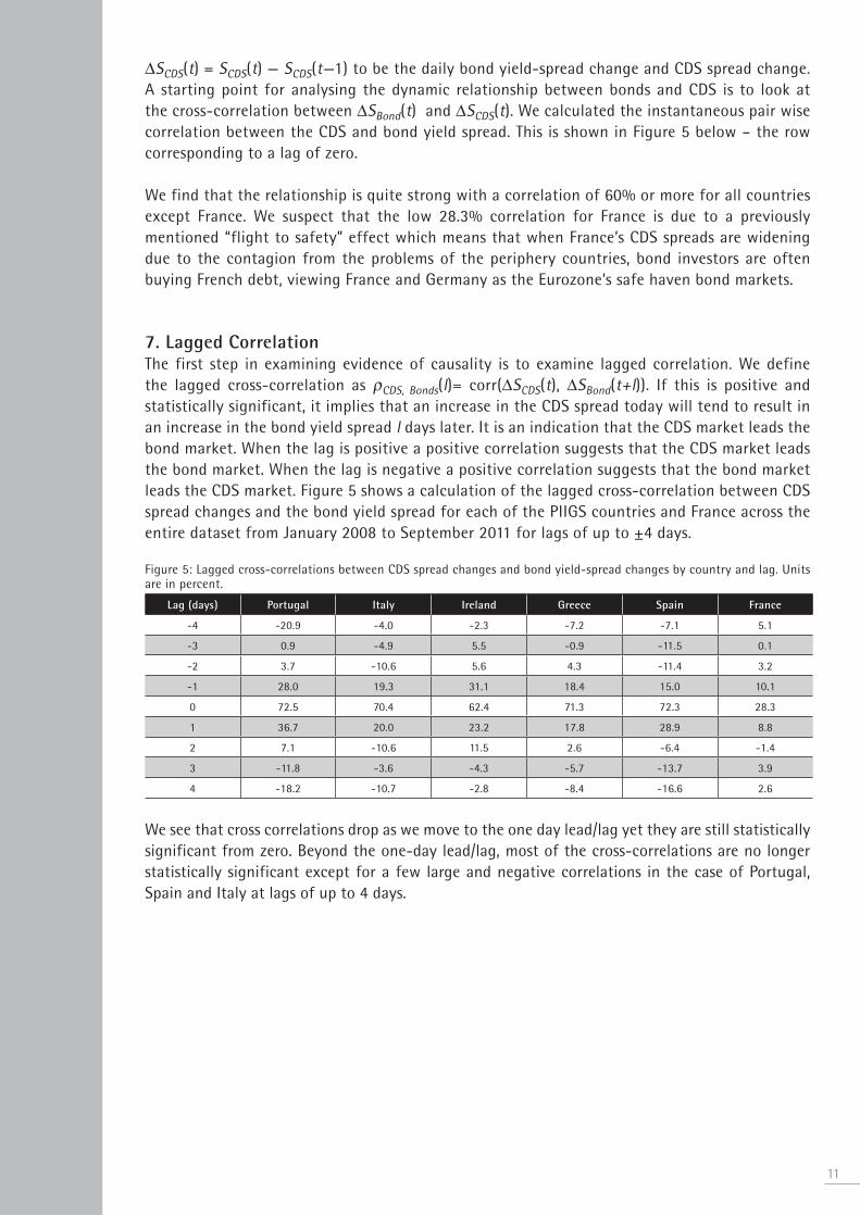
7. Lagged CorrelationThe first step in examining evidence of causality is to examine lagged correlation. We define the lagged cross-correlation as ρCDS, Bonds(l)= corr(∆SCDS(t), ∆SBond(t+l)). If this is positive and statistically significant, it implies that an increase in the CDS spread today will tend to result in an increase in the bond yield spread l days later. It is an indication that the CDS market leads the bond market. When the lag is positive a positive correlation suggests that the CDS market leads the bond market. When the lag is negative a positive correlation suggests that the bond market leads the CDS market. Figure 5 shows a calculation of the lagged cross-correlation between CDS spread changes and the bond yield spread for each of the PIIGS countries and France across the entire dataset from January 2008 to September 2011 for lags of up to ±4 days.

Figure 5: Lagged cross-correlations between CDS spread changes and bond yield-spread changes by country and lag. Units are in percent.

Lag (days) Portugal Italy Ireland Greece Spain France

-4 -20.9 -4.0 -2.3 -7.2 -7.1 5.1

-3 0.9 -4.9 5.5 -0.9 -11.5 0.1

-2 3.7 -10.6 5.6 4.3 -11.4 3.2

-1 28.0 19.3 31.1 18.4 15.0 10.1

0 72.5 70.4 62.4 71.3 72.3 28.3

1 36.7 20.0 23.2 17.8 28.9 8.8

2 7.1 -10.6 11.5 2.6 -6.4 -1.4

3 -11.8 -3.6 -4.3 -5.7 -13.7 3.9

4 -18.2 -10.7 -2.8 -8.4 -16.6 2.6

We see that cross correlations drop as we move to the one day lead/lag yet they are still statistically significant from zero. Beyond the one-day lead/lag, most of the cross-correlations are no longer statistically significant except for a few large and negative correlations in the case of Portugal, Spain and Italy at lags of up to 4 days.

11

12

Figure 6: The CDS basis over time quoted as the CDS spread minus the bond yield spread.

The time series of both yield-spread and CDS spread changes exhibited a number of large daily movements or jumps, in both the positive and negative direction. We tested the extent to which our results were due to such jumps. We first recalculated these lagged correlations after capping all daily spread moves with a magnitude greater than some threshold, thereby reducing the impact of large jumps. We found that this reduced synchronous correlations. This was explained by an examination of the data which showed that there were a number of days associated with Eurozone debt crisis15 on which CDS and bond markets moved synchronously and by a large amount. In the case of Greece, the synchronous correlation between CDS and bond spread changed fell from 71.5% to 51.7% when using a maximum daily jump of 50bp. It also increased the 1-day lagged cross correlation from around 18% to 28%. As a second test, we calculated the lagged correlations but only allowing spread movements with a magnitude greater than some threshold, thereby only including jumps. We found that selecting for jumps only increased the zero lag cross-correlations for the reasons described previously. In both sets of tests, we found that the lagged correlation numbers did change, but that the sign and magnitude of the auto and cross-correlation statistics did not change materially when capping jumps or only including jumps. This suggested that the same underlying market dynamics were driving both the small and large spread movements.

8. Granger Causality TestIf the measured lagged correlations are positive and statistically significant from zero, we can infer that some temporal relationship exists. To examine this we can test for the presence of Granger causality. A Granger causality test is a more powerful indicator of causality than the lagged cross-correlation as it determines whether there is a flow of information from one variable to another, and the direction in which it travels.

Before examining Granger causality we must determine whether or not the CDS and bond yield spread processes exhibit co-integration. This occurs when two integrated I(1) processes can be combined linearly to create a process with a long term equilibrium relationship. Figure 7 shows the evolution of the simple CDS basis SCDS(t) — SBond(t) through time and we wish to know if this

15 - These include the following dates 27 April 2010 (period following Moody’s downgrade of Greece), 10 May 2010 (EU and IMF agree emergency fund), 20-21 July 2011 (initial Greek restructuring deal).

time series, or any linear combination of the CDS and bond yield spreads, exhibits a long term relationship. Existence of co-integration would suggest the use of an error correction model (ECM) as a more appropriate model choice for the dynamics of the CDS and bond spreads.

Figure 7: ADF test results for a unit root for the CDS and bond yield spreads. The null hypothesis of a unit root is not rejected in all cases

Augmented Dickey-Fuller t-statistic

Country CDS Spreads Bond Yield Spreads

Portugal 1.479 0.910

Italy 0.810 0.392

Ireland 0.298 -0.631

Greece 2.231 2.039

Spain 0.803 0.111

France 1.154 -0.743

To test for co-integration we must first determine whether or not the CDS and bond yield spread processes used in this analysis have a unit root, i.e. that they are non-stationary integrated processes. We did this using the Augmented Dickey-Fuller (ADF) statistic and the results are shown in Figure 7. The more negative the ADF statistic, the stronger the rejection of the hypothesis that the process is and the unit root is rejected. We conclude from these results that the unit root hypothesis was not rejected for any of the CDS or bond yield-spread processes.

We then used the augmented Dickey-Fuller (ADF) statistic to test for co-integration on a linear combination of CDS and bond-yield spreads. Co-integration requires that there is a linear combination of the two spread processes which does not have a unit root and so is therefore stationary, i.e. it would reject the ADF null hypothesis of a unit root. For this to occur we need to find an ADF t-statistic which is less than the critical value at some confidence level. From our analysis, we found that the ADF t-statistics for all countries were negative as shown in Figure 8. However, given that the 1% critical value was -3.88 and the 10% critical value was -3.04, the null hypothesis of a unit root was only rejected at the 90% confidence level by France and at the 99% confidence level by Spain. These results suggest that the relationship between Spanish CDS and bond yield-spreads and between French CDS and bond yield-spreads may exhibit cointegration. However at these confidence levels, the possibility of cointegration is ruled out for the other countries. We therefore did not build an ECM but performed a Granger causality test on the lagged processes.16

Figure 8: The co-integrated Dickey-Fuller t-statistic for CDS and bond yield-spreads. The null hypothesis is that the process has a unit root. This is only rejected at 1% by Spain and at 10% by France.15

Portugal Italy Ireland Greece Spain France

-2.59 -2.95 -2.67 -2.70 -3.92 -3.04

The Granger test makes it possible to test for causality in both directions – i.e. from bonds to CDS and vice-versa. The first step of the Granger causality test was to determine the number m of lags for the CDS spread changes time series by regressing ∆SCDS(t) against its lagged values back to ∆SCDS(t—m) and choosing the regression with the number of lags which optimises the Bayesian Information Criterion (BIC). We then determined the optimal number of lags n of time series ∆SBond(t) by regressing ∆SCDS(t) against its m lagged values and the n lagged values of ∆SBond(t). Once again we chose the regression with the value of n which optimises the BIC. In all optimisations we allowed a maximum lag of 5 days. The underlying model equation is:

1316 - We included France and Spain in this, although we must caveat this by acknowledging that the possible existence of cointegration in their time series may produce spurious results. Due to time constraints we do not examine the properties of an ECM for France and Spain.

14

We then tested the null hypothesis which is that the lagged values of ∆SBond do not Granger cause ∆SCDS(t). Formally, this is the test that β1 = β2 =… = βn = 0. A deviation from this with statistical significance as measured using an F-statistic allows us to accept or reject this null hypothesis. We set a significance level of 0.1% for rejection of the hypotheses. We then repeated this exercise with the model equation

in an attempt to see if CDS spread changes Granger cause bond spread changes. The results are shown in Figure 9.

Figure 9: Results of the Granger test showing the F-statistic, p-statistic and the optimal number of lags based on the BIC criterion.

Null Hypothesis CDS do not lead bonds Bonds do not lead CDS

Country F-statistic P-statistic

(%)

Optimal

Lags m/n

Accept/

Reject

F-statistic P-statistic

(%)

Optimal

Lags m/n

Accept/

Reject

Portugal 33.7 0.0 4/3 R 16.5 0.0 5/4 R

Italy 5.3 2.2 4/1 A 10.8 0.0 2/2 R

Ireland 16.3 0.0 5/3 R 19.2 0.0 1/1 R

Greece 32.6 0.0 1/1 R 2.92 8.8 1/1 A

Spain 27.1 0.0 2/1 R 5.49 1.9 5/1 A

France 4.76 3.1 1/1 A 47.9 0.0 5/1 R

A rejection of a hypothesis to 99.9% significance is signalled by a p-statistic lower than 0.1%. Our results show that there are three categories of country and mutual causality relationship. We find that: (i) in Greece and Spain, CDS spread changes Granger cause changes in the bond yield spreads but bond yield changes do not Granger cause CDS spread changes; (ii) in Italy and France, bond yield spread changes Granger cause CDS spread changes but CDS spread changes do not Granger cause bond yield spread changes; and (iii) in Portugal and Ireland, CDS spread changes and bond yield spread changes lead each other, a result which can be interpreted as a feedback. We note that most of the Granger causing lags represented by the value of n were at just one day suggesting that any information transfer effect is short-lived.

ConclusionsA theoretical model-based analysis of the relationship between CDS spreads and bond yield spreads shows that CDS spreads generally trade wide to bond yield spreads, especially when the expected recovery rate assumption is greater than zero. Currency effects due to the dollar denomination of CDS protection can also cause the quoted par CDS spread to trade wider than the comparable bond yield. Therefore a positive CDS basis, measured as the CDS spread minus the bond yield spread, is not in itself a sign that the CDS and bond markets are dislocated and certainly not a sign of speculative activity. A model is needed to determine when there is a theoretical mispricing and even if there is, the mispricing may not be arbitrageable.

Empirical analyses of the relationship between CDS spreads and bond yield-spreads show that the market only obeys the theoretical model implied relationship in a very approximate way. One reason why this relationship is not strictly observed is that the the model-implied arbitrage is not even approximately a tradable arbitrage when the credit risky bond is pricing away from par. This means that market participants will only act on theoretical arbitrages when dislocations become large enough to make the risk-return profile of the trade attractive. An additional factor which could be material in causing CDS and bond spreads to diverge, and which we have discussed, is the denomination of market-standard CDS contracts on European sovereign debt in dollars while the reference obligations are denominated in euro. If the market anticipates that the euro will fall in value following a sovereign default, the cost of

buying CDS protection in dollars will be higher than the cost assuming no currency impact, and vice-versa.

We find that lagged values of changes in the CDS spread and changes in the bond yield spread exhibit both autocorrelation and cross-correlation, with the greatest effect occurring at a lag of one day. These correlations were especially significant for the sovereigns which experienced the greatest spread widening17 over the sample period. Granger causality tests can give us indications of the direction of any information flow and the results of our Granger causality tests were mixed. They suggested that the dominant direction of causality is from CDS to bonds for Greece, but from bonds to CDS for France and Italy, while Ireland and Portugal exhibited Granger causality in both directions, implying a feedback system. We emphasise that a positive test for Granger causality is not evidence of true causality. However while a negative test would rule out the hypothesis of true causality, a positive test tells us that we cannot currently reject such a hypothesis.

ThanksThe author thanks Sergio Focardi, Joelle Miffre, Douglas Keenan and Lutz Schloegl for helpful comments.

AppendixThe default time τ of the reference credit is modelled as the first stopping time of a Poisson process with intensity λ(t) . Using a simple model of a fixed coupon bond with N remaining full coupon periods consisting of a coupon c paid with frequency ƒ we find that the time zero bond price is given by

where r(t) is the default-free short-rate process at time t and R(τ) is the realised recovery rate in the event of default at time τ. We take the expectation in the risk-neutral Q-measure. We assume that on default, all future coupon payments are lost and the recovery is a fixed percentage of the face value of the bond. Assuming independence between interest rates and the intensity process lambda, we can write the bond price as

where

is the survival probability of the reference credit to time t.

15 17 - Portugal, Ireland and Greece.

16

References• Adler, M., and J. Song, (2007). The Behaviour of Emerging Market Sovereigns Credit Default Swap Premiums and Bond Yield Spreads, Working Paper.

• Baltagi, B.H., (2011). Econometrics, 5th Edition, Springer-Verlag.

• Blanco, R., S. Brennan and I. Marsh (2003). An empirical analysis of the dynamic relationship between investment-grade bonds and credit default swaps, Bank of England Working Paper No. 211

• Calice, G., J. Chen and J. Williams (2011). Liquidity Spillovers in Sovereign Bond and CDS Markets, Working paper.

• Das, S., M. Kalimpalli and S. Nayak (2011). Did CDS Trading Improve the Market for Corporate Bonds, Working paper.

• Duffie, D. (1999). Credit Swap Valuation, Financial Analysts Journal, January/February 1999

• O’Kane, D. and R. McAdie (2001). Explaining the Basis: Cash versus Default Swaps, Lehman Brothers Fixed Income Research.

• O’Kane, D. (2008). Modelling Single-name and Multi-name credit derivatives, Wiley Finance.