the liquidity trap, the real balance effect, and the friedman rule∗ boston
TRANSCRIPT

INTERNATIONAL ECONOMIC REVIEWVol. 46, No. 4, November 2005
THE LIQUIDITY TRAP, THE REAL BALANCE EFFECT,AND THE FRIEDMAN RULE∗
BY PETER N. IRELAND1
Boston College and National Bureau of Economic Research, U.S.A.
This article studies the behavior of the economy and the efficacy of monetarypolicy under zero nominal interest rates using a model with population growththat nests, as a special case, the conventional specification in which there is a singleinfinitely lived representative agent. The article shows that with a growing pop-ulation, monetary policy has distributional consequences that give rise to a realbalance effect, thereby eliminating the liquidity trap. These same distributionaleffects, however, can also work to make many agents much worse off under zeronominal interest rates than they are when the nominal interest rate is positive.
1. OLD IDEAS, NEW MODELS
Inflation has come full circle. Low before 1960, it rose during the 1960s andpeaked during the 1970s. From this peak, it fell during the 1980s, finally stabiliz-ing during the 1990s at levels very similar to those prevailing before 1960. Thissame circular pattern appears in data from virtually all the major industrializedcountries—in North America, in Europe, and in Asia—as shown, for example, byMussa (2000, Table 1, p. 1103).
Monetary economists and central bankers have also come full circle. Concernedmainly with halting and reversing inflation’s upward trend during the 1970s and1980s, analysts and policymakers have more recently rediscovered some of thespecial problems that can arise under conditions of price stability. These problemsreceived much attention long ago but were ignored for more than a generation.Now they have taken center stage once again.
Chief among these problems are those associated with the liquidity trap, whichaccording to Hicks (1937) lies at the core of Keynes’ (1936) economics. Krugman(1998) and Svensson (1999) reconsider the idea of the liquidity trap using state-of-the-art monetary models in which optimizing agents have rational expectations.In both Krugman’s cash-in-advance model and Svensson’s money-in-the-utility
∗ Manuscript received June 2003; revised August 2004.1 I would like to thank Kevin Moran, Randy Wright, two anonymous referees, participants in the
November 2002 meeting of the Canadian Macro Study Group at Queen’s University, and participantsin seminars at Emory University, the Federal Reserve Board, and the University of Mississippi for veryhelpful comments and suggestions. This material is based upon work supported by the National ScienceFoundation under Grant No. SES-0213461. Any opinions, findings, and conclusions or recommenda-tions expressed herein are my own and do not reflect those of the National Bureau of Economic Re-search or the National Science Foundation. Please address correspondence to: Peter N. Ireland, BostonCollege, Department of Economics, 140 Commonwealth Avenue, Chestnut Hill, MA 02467-3859,USA; Tel: (617) 552-3687. Fax: (617) 552-2308. E-mail: [email protected]. http://www2.bc.edu/irelandp.
1271

1272 IRELAND
function model, households become willing to hoard any additional money thatthe government chooses to supply after the nominal interest rate reaches its lowerbound of zero. The central bank then loses control of the price level and perhapsother key variables as well.
Notably absent from these new models of the liquidity trap, however, is anotherold idea: that of the real balance effect. First discussed by de Scitovszky (1941),Haberler (1946), and Pigou (1943) and developed most extensively by Patinkin(1965), the real balance effect describes a channel through which a change in realbalances, caused either by a change in the nominal money supply or a change inthe nominal price level, impacts on household wealth and thereby affects con-sumption and output. The real balance effect allows the central bank to influencethe economy even after the nominal interest rate hits its lower bound. Yet thiseffect appears nowhere in Krugman and Svensson’s analyses. Why?
It has been widely appreciated, since the publication of Barro’s (1974) famousarticle on Ricardian equivalence, that government bonds will not be perceivedas a source of private-sector wealth if the households owning those bonds arethe same households that must pay all of the taxes that will eventually be used toretire the government’s debt. Less widely appreciated, however, is a closely relatedfinding, presented most explicitly by Weil (1991) but also implicit in earlier work bySachs (1983) and Cohen (1985). These authors show that government-issued fiatmoney will not be perceived as a source of private-sector wealth if the householdsowning that money are the same households that, first, receive all of the transfersor pay all of the taxes associated with future changes in the money supply and that,second, incur all of the opportunity costs associated with carrying the money stockbetween all future periods. In fact, Krugman and Svensson’s representative–agentmodels describe environments in which money is not net wealth. In these models,therefore, the real balance effect disappears.
This article extends Krugman’s cash-in-advance framework by introducinggrowth in the number of infinitely lived households as modeled by Weil. Thearticle shows that with a growing population, households alive in the present payonly a fraction of the taxes levied in the future when the government choosesto contract the money supply. Money becomes net wealth and, consequently, anoperative real balance effect gives the central bank control over the price leveleven when the nominal interest rate equals zero. Only in the special case withoutpopulation growth—the special case in which the more general model developedhere collapses to Krugman’s original specification—does the liquidity trap survive.
Introducing population growth in the manner suggested by Weil also servesto resolve a second puzzle that emerges out of Krugman and Svensson’s earlieranalyses. By associating the case of zero nominal interest rates with the Keynesianliquidity trap, Krugman and Svensson conjure up images of terrible economicoutcomes: the Great Depression in the United States or the ongoing lengthyand severe recession in Japan. As emphasized by Cole and Kocherlakota (1998),however, zero nominal interest rates in models such as Krugman and Svensson’sare actually associated with highly desirable resource allocations. In fact, zeronominal interest rates in these models are linked more closely to Friedman’s(1969) rule for the “Optimum Quantity of Money” than to what Hicks (1937,

THE REAL BALANCE EFFECT 1273
p. 155) calls the “Economics of Depression.” But are zero nominal interest ratesalways good for the economy?
Weiss (1980), Freeman (1985, 1989, 1993), and Smith (2002) all present ex-amples of overlapping generations models in which the Friedman rule fails tomaximize private agents’ steady-state utility. Bhattacharya et al. (2004) unify andexplain these results by tracing them back to distributional effects that are absentin representative-agent models like Krugman and Svensson’s. This article alsoshows that distributional effects—the same distributional effects, as a matter offact, that give rise to the real balance effect—operate once population growth isintroduced into Krugman’s cash-in-advance model. Here, these distributional ef-fects can make virtually all households much worse off under zero nominal interestrates than they are when interest rates are positive.
On the other hand, Bhattacharya et al. also demonstrate that in overlappinggenerations models, the Friedman rule’s optimality is typically restored when off-setting fiscal transfers are used to neutralize the distributional effects that defla-tionary policies would otherwise have.2 This result, too, carries over to the modelwith growth in the number of infinitely lived household studied here. In the end,therefore, this article joins with Bhattacharya et al. by suggesting that the prin-cipal dangers posed by deflationary policies have little to do with zero nominalinterest rates per se and even less to do with the Keynesian liquidity trap. Rather,both the problems and their ultimate solutions lie in the mechanics through whichdeflationary policies are implemented.
2. AN EXTENDED CASH-IN-ADVANCE MODEL
2.1. Overview. Here, Weil’s (1991) continuous-time, money-in-the-utilityfunction model with a growing number of infinitely lived households is recast as adiscrete-time, cash-in-advance model. Weil’s original specification assigns to eachhousehold a utility function that is strictly increasing in two arguments: consump-tion and real money balances. Since households cannot be satiated by any finitestock of real balances, equilibria in Weil’s original model exist only under strictlypositive nominal interest rates, ruling out an analysis of the case that Krugman(1998) associates with the liquidity trap. Of course, one could also modify Weil’smodel in a manner consistent with Svensson (1999) by introducing a satiationpoint beyond which the marginal utility of real balances equals zero. The cash-in-advance framework used here, however, incorporates the satiation point for realbalances in a way that is linked more naturally to the volume of each household’snominal expenditures.
Whitesell (1988) presents a model that is quite similar to Weil’s and uses thatmodel to study the effects of money growth on the capital stock and welfare. Infact, both Weil’s model and Whitesell’s can be viewed as extensions of Blanchard’s(1985) model of finite horizons. In Blanchard’s model, each agent faces a constantprobability of death; meanwhile, newly born agents arrive at a rate that keeps the
2 As noted below, Abel (1987) and Gahvari (1988) present earlier examples of Bhattacharya et al.’sgeneral result.

1274 IRELAND
total population constant. Buiter (1988) generalizes Blanchard’s model so as tobreak the tight link between birth and mortality rates. Buiter’s analysis revealsthat it is the arrival of newly born agents, rather than the finite horizons of exist-ing agents, that is essential in overturning Barro’s (1974) Ricardian equivalenceresult—a result that, as noted above, relates closely to the presence or absenceof monetary wealth effects. Thus, the model used here, like the models used byWeil and Whitesell, retains the essential feature of population growth in an envi-ronment where all agents are infinitely lived. And conveniently, this more generalmodel nests, as the special case in which the population growth rate equals zero,the conventional specification that features a single infinitely lived representativeagent.
Weil’s model, in which goods are received by each household in the form of aconstant endowment, is also extended here by allowing each household to pro-duce output with labor. Here, as in Wilson (1979), Cooley and Hansen (1989),Cole and Kocherlakota (1998), and Ireland (2003), positive nominal interest ratesdistort households’ labor supply decisions. Thus, the structure of production andtrade gives rise to a mechanism that might make the central bank want to followthe Friedman (1969) rule, which provides for zero nominal interest rates. And, in-deed, the Friedman rule is optimal in the special case where the population growthrate equals zero. When the population grows at a positive rate, however, the taxesthat the government must levy to implement the Friedman rule generate distri-butional effects that can make zero nominal interest rates quite costly for manyagents.
2.2. Demographic Structure. A new cohort of infinitely lived households isborn at the beginning of each period t = 0, 1, 2, . . . . Those households born in aparticular period t = s belong to cohort s. The arrival of new cohorts causes thetotal number of households to grow at the constant rate n ≥ 0. Let Nt denote thenumber of households alive during period t. Then given N0 > 0,
Nt+1 = (1 + n)Nt
for all t = 0, 1, 2, . . . .Households of a given cohort are identical, so that it is possible to consider a
representative household for each cohort. The representative household of cohorts has preferences described by the utility function
∞∑t=s
β t−s ln[cs
t − (1/γ )(hs
t
)γ ](1)
where 1 > β > 0, γ > 1, c st denotes the household’s consumption, and hs
t denotesthe household’s hours worked during period t. This specification for utility impliesthat the marginal rate of substitution between consumption and hours workeddepends only on hours worked, so that in particular there are no wealth effectson labor supply. Here, this special assumption greatly simplifies the aggregation

THE REAL BALANCE EFFECT 1275
of quantities chosen by households of different cohorts having different levels ofaccumulated financial wealth.3
Thus, during any given period, the economy consists of many infinitely livedagents of varying ages. As suggested by Weil (1991) and Whitesell (1988), there-fore, the population growth rate n serves as a measure of financial disconnected-ness and heterogeneity in the economy as a whole. In the special case with n = 0,however, the model collapses to the more familiar one in which there is a singleinfinitely lived representative agent.
2.3. Timing of Events. The representative household of cohort s enters eachperiod t = s, s + 1, s + 2, . . . , with money Ms
t and bonds Bst . Only the initial
cohort is endowed with money at birth, and no cohort is endowed with bondsat birth, so that M0
0 > 0 but Mss = 0 for all s = 1, 2, 3, . . . , and Bs
s = 0 for alls = 0, 1, 2, . . . . As emphasized by Weil (1991) and Whitesell (1988), these initialconditions formalize the idea that newly born households are not linked financiallyto previously existing dynasties.
The representative household of each cohort s receives a lump-sum monetarytransfer T s
t from the central bank at the beginning of each period t = s, s + 1,s + 2, . . . . Also at the beginning of each period, existing bonds mature, providingthe representative household of cohort s with Bs
t additional units of money. Thehousehold uses some of its money to purchase Bs
t+1 new bonds at the price of1/(1 + r t) units of money per bond, where rt denotes the net nominal interest ratebetween t and t + 1; the household carries the rest of its money into the goodsmarket.
The description of goods production and trade builds on Lucas’ (1980) interpre-tation of the cash-in-advance model. Each household consists of two members: ashopper and a worker. The shopper from the representative household of cohorts purchases c s
t units of output from workers from other households, subject to thecash-in-advance constraint
Mst + Ts
t + Bst − Bs
t+1
/(1 + rt ) ≥ Pt cs
t(2)
where Pt denotes the nominal price of goods during period t. Meanwhile, theworker from the representative household of cohort s uses hs
t units of labor toproduce ys
t units of output according to the constant-returns-to-scale technologythat yields one unit of output for every unit of labor input,
yst = hs
t
The worker sells this output to shoppers from other households for Pthst units of
money. The representative household’s two members then reunite to consume the
3 Although this specification for utility is also used by Greenwood et al. (1988), among others, ithas sometimes been criticized for being inconsistent with balanced growth in models with rising realwages driven by exogenous technological progress. Along these lines, however, Greenwood et al.(1995) demonstrate that a very similar utility function that does remain consistent with balancedgrowth emerges from a model with home production when productivity rises at the same average rateacross the market and household sectors. For simplicity, however, the model used here abstracts fromtechnological progress all kinds.

1276 IRELAND
shopper’s purchases. The household carries Mst+1 units of money into period t +
1; its choices must satisfy the budget constraint
Mst + Ts
t + Bst + Pt hs
t ≥ Pt cst + Bs
t+1
/(1 + rt ) + Ms
t+1(3)
In addition to the cash-in-advance and budget constraints (2) and (3), whichmust hold for all t = s, s + 1, s + 2, . . . , the representative household’s choicesmust satisfy a set of nonnegativity constraints
hst ≥ 0, Ms
t+1 ≥ 0, cst − (1/γ )
(hs
t
)γ> 0(4)
for all t = s, s + 1, s + 2, . . . . The first two constraints in (4) are standard; the thirdmust be imposed given the special form of the utility function (1).
The representative household of cohort s can borrow by choosing negativevalues for Bs
t+1 but is not allowed to engage in Ponzi schemes through which itborrows more than it can ever repay. To formalize the constraints that rule outsuch Ponzi schemes, let Q0 = 1 and
Qt =t−1∏u=0
(1
1 + ru
)
for all t = 1, 2, 3, . . . . Then for any T ≥ t ≥ 0, QT/Qt measures the presentdiscounted value at the beginning of period t of one unit of money received at thebeginning period T. The no-Ponzi-scheme constraints are
Wst+1 = Ms
t+1 + Bst+1 +
∞∑u=t+1
(Qu/Qt+1)(Ts
u + Puhsu
) ≥ 0(5)
for all t = s, s + 1, s + 2, . . . . Part 1 of the appendix shows that these no-Ponzi-scheme constraints imply that the infinite-horizon budget constraint
Qt(Ms
t + Bst
) +∞∑
u=t
Qu(Ts
u + Puhsu
) ≥∞∑
u=t
Qu
[Pucs
u +(
ru
1 + ru
)Ms
u+1
](6)
applies to the household’s choices from period t forward. This infinite-horizon bud-get constraint includes, as sources of funds, the household’s beginning-of-periodnominal balances Ms
t as well as the present discounted value of the monetary trans-fers that the household receives from period t forward. It also includes, as usesof funds, the present discounted value of the opportunity costs that the house-hold incurs when it carries money instead of bonds between all future periods.Ultimately, a comparison between the values of these three items will determinewhether or not the real balance effect is operative in general equilibrium.
2.4. Household Optimization. Taking the initial conditions Mss and Bs
s asgiven, the representative household of cohort s chooses sequences {c s
t , hst , Ms
t+1,Bs
t+1}∞t=s to maximize the utility function (1) subject to the constraints (2)–(5),
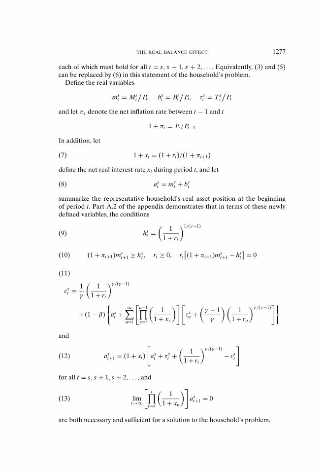
THE REAL BALANCE EFFECT 1277
each of which must hold for all t = s, s + 1, s + 2, . . . . Equivalently, (3) and (5)can be replaced by (6) in this statement of the household’s problem.
Define the real variables
mst = Ms
t
/Pt , bs
t = Bst
/Pt , τ s
t = Tst
/Pt
and let π t denote the net inflation rate between t − 1 and t
1 + πt = Pt/Pt−1
In addition, let
1 + xt = (1 + rt )/(1 + πt+1)(7)
define the net real interest rate xt during period t, and let
ast = ms
t + bst(8)
summarize the representative household’s real asset position at the beginningof period t. Part A.2 of the appendix demonstrates that in terms of these newlydefined variables, the conditions
hst =
(1
1 + rt
)1/(γ−1)
(9)
(1 + πt+1)mst+1 ≥ hs
t , rt ≥ 0, rt[(1 + πt+1)ms
t+1 − hst
] = 0(10)
cst = 1
γ
(1
1 + rt
)γ /(γ−1)
+ (1 − β)
{as
t +∞∑
u=t
[u−1∏v=t
(1
1 + xv
)] [τ s
u +(
γ − 1γ
) (1
1 + ru
)γ /(γ−1)]}
(11)
and
ast+1 = (1 + xt )
[as
t + τ st +
(1
1 + rt
)γ /(γ−1)
− cst
](12)
for all t = s, s + 1, s + 2, . . . , and
limt→∞
[t∏
v=s
(1
1 + xv
)]as
t+1 = 0(13)
are both necessary and sufficient for a solution to the household’s problem.
1278 IRELAND
Equation (9) confirms that positive nominal interest rates distort the house-hold’s labor supply decisions, as discussed by Wilson (1979), Cooley and Hansen(1989), Cole and Kocherlakota (1998), and Ireland (2003). Equation (10) restatesthe cash-in-advance constraint. It reveals that when the nominal interest rate hitsits lower bound of zero, the cash-in-advance constraint no longer binds; this is thecase that Krugman (1998) associates with the liquidity trap.
Equation (11) defines the household’s consumption function, which accordingto the permanent income hypothesis links consumption to total wealth. Embeddedinto the right-hand side of (11) are the same three components of monetary wealthidentified in (6): the household’s current money balances, the present discountedvalue of the future monetary transfers, and the present discounted value of theopportunity costs associated with carrying money instead of bonds between futureperiods. Once again, a comparison between the values of these three items willdetermine whether or not the real balance effect appears in equilibrium.
Equation (12) governs the evolution of the household’s financial wealth. Itshows that the household accumulates wealth as it earns interest on its existingassets and as it receives monetary transfers from the government; the householdalso accumulates wealth by working more and consuming less. Finally, (13) is thehousehold’s transversality condition. If the limit on the left-hand side of (13) wasnegative, then the household would be violating the no-Ponzi-scheme constraintsin (5); if, on the other hand, the limit was positive, then the household couldachieve a preferred consumption profile, without violating any of its constraints,by drawing down its stock of financial assets.
2.5. Aggregation. Define aggregate per household financial wealth during pe-riod t as
at = N0 a0t + ∑t
s=1(Ns − Ns−1)ast
Nt
and define aggregate per household real money balances mt, real bond holdingsbt, hours worked ht, and consumption ct similarly. Also, and importantly, let
τt = N0τ0t + ∑t
s=1(Ns − Ns−1)τ st
Nt
denote aggregate per household real money transfers made to all agents aliveduring period t and let
τu,t = N0τ0u + ∑t
s=1(Ns − Ns−1)τ su
Nt
denote aggregate per household real monetary transfers made during periodu ≥ t to those households that were alive during period t. Then, of course, τ t,t =τ t for all t = 0, 1, 2, . . . . But for u = t + 1, t + 2, t + 3, . . . , τ u,t will generally differ

THE REAL BALANCE EFFECT 1279
from τ u, since some of the monetary transfers made during period u may go tohouseholds born during periods t + 1 through u.
In terms of these aggregates, (8)–(12) become
at = mt + bt(14)
ht =(
11 + rt
)1/(γ−1)
(15)
(1 + n)(1 + πt+1)mt+1 ≥ ht , rt ≥ 0, rt [(1 + n)(1 + πt+1)mt+1 − ht ] = 0(16)
ct = 1γ
(1
1 + rt
)γ /(γ−1)
+ (1 − β)
{at +
∞∑u=t
[u−1∏v=t
(1
1 + xv
)] [τu,t +
(γ − 1
γ
) (1
1 + ru
)γ /(γ−1)]}
(17)
and
at+1 =(
1 + xt
1 + n
) [at + τt +
(1
1 + rt
)γ /(γ−1)
− ct
](18)
for all t = 0, 1, 2, . . . . Although (14)–(16) are straightforward analogs to (8)–(10), acomparison of (17) to (11) reveals that aggregate per household consumption dur-ing period t depends on the real value of future monetary transfers, but only to theextent that those transfers will be made to households that are alive during periodt. Similarly, a comparison of (18) to (12) suggests that aggregate per householdfinancial wealth tends to grow at a slower rate than each individual household’sfinancial wealth, since newly born households start their lives without money andbonds.
2.6. Equilibrium Conditions. Equations (7) and (14)–(18) form a system ofsix equations in the 10 aggregate variables xt, r t, π t+1, at, mt, bt, ht, ct, τ t , and τ u,t.This system can be closed by imposing the market-clearing conditions for goodsand labor,
ht = ct(19)
for all t = 0, 1, 2, . . . , and by making assumptions about the government’s supplyof money and bonds.

1280 IRELAND
Accordingly, suppose first that the government issues no bonds. Then, in equi-librium,
bt = 0(20)
must also hold for all t = 0, 1, 2, . . . . Note that (20) only requires that aggregateper household bonds equal zero; it does not rule out the possibility that for anyindividual household, b s
t will be nonzero as households of different cohorts borrowand lend among themselves by trading bonds.
Suppose next that the government acts to expand the total nominal moneysupply at the constant rate σ by making equal lump-sum transfers to all householdsalive during each period. Then, in equilibrium,
τt = σmt(21)
and
τu,t = σmu(22)
will hold for all t = 0, 1, 2, . . . , and u = t , t + 1, t + 2, . . . .Under government policies described by (20)–(22), (14) immediately implies
that
at = mt(23)
whereas (7) and (15)–(18) become
1 + xt = (1 + rt )/(1 + πt+1)(24)
ct =(
11 + rt
)1/(γ−1)
(25)
(1 + n)(1 + πt+1)mt+1 ≥ ct , rt ≥ 0, rt [(1 + n)(1 + πt+1)mt+1 − ct ] = 0(26)
ct = 1γ
(1
1 + rt
)γ /(γ−1)
+ (1 − β)
{mt +
∞∑u=t
[u−1∏v=t
(1
1 + xv
)] [σmu +
(γ − 1
γ
) (1
1 + ru
)γ /(γ−1)]}
(27)
and
mt+1 =(
1 + xt
1 + n
) [(1 + σ )mt +
(1
1 + rt
)γ /(γ−1)
− ct
](28)

THE REAL BALANCE EFFECT 1281
for all t = 0, 1, 2, . . . . Given the government’s choice of the money growth rateσ , (24)–(28) determine the equilibrium behavior of the five aggregate variablesxt, r t, π t+1, mt, and ct; paths for the remaining five aggregates at, bt, ht, τ t , and τ u,t
then follow immediately from (19)–(23).
2.7. Steady-State Equilibria. Equations (24)–(28) imply that under a policy ofconstant money growth σ via equal lump-sum transfers, a steady-state equilibriumexists in which aggregate variables are constant over time, with xt = x, r t = r , π t+1 =π , mt = m, and ct = c for all t = 0, 1, 2, . . . .4 Part A.3 of the appendix demonstratesthat, more specifically, (24)–(28) require the five steady-state values x, r , π , m, andc to satisfy
1 + x = (1 + r)/(1 + π)(29)
1 + π = (1 + σ )/(1 + n)(30)
c =(
11 + r
)1/(γ−1)
(31)
(1 + σ )m ≥ c, r ≥ 0, r [(1 + σ )m − c] = 0(32)
and
c = 1γ
(1
1 + r
)γ /(γ−1)
+ (1 − β)
{[1 +
(1 + x
x
)σ
]m +
(γ − 1
γ
) (1 + x
x
) (1
1 + r
)γ /(γ−1)}
(33)
Equation (29) defines the steady-state real interest rate as the difference be-tween the nominal interest rate and the inflation rate; similarly, (30) determinesthe steady-state inflation rate as the difference between the money growth rateand the population growth rate. Equation (31) confirms that across steady-stateequilibria, higher nominal interest rates reduce consumption and output as wellas employment. Equation (32), derived from the cash-in-advance constraint, de-scribes the aggregate demand for money, and (33) is the aggregate consumptionfunction with the steady-state conditions imposed.
4 In addition, (24)–(28) characterize the model’s dynamics away from the steady state. As notedbelow, however, this model has no predetermined state variables: Hence, if a steady state exists, aperfect foresight equilibrium also exists in which the economy begins and remains forever in that steadystate. A more thorough analysis of the model’s dynamics would therefore serve only to confirm or ruleout the existence of multiple perfect foresight equilibria of the kind studied in a more conventionalcash-in-advance specification by Woodford (1994).
1282 IRELAND
3. THE LIQUIDITY TRAP AND THE REAL BALANCE EFFECT
What do the steady-state conditions (29)–(33) imply about the behavior of theeconomy and the efficacy of monetary policy under zero nominal interest rates?To answer this question, it is helpful to consider two cases. The first case setsn = 0, so that there is no population growth. This first case is therefore the specialcase in which the more general model developed here reduces to the familiarspecification, used by Krugman (1998) and many others, in which there is a singlerepresentative agent. And, indeed, Krugman’s liquidity trap appears in this specialcase: The central bank loses control over the price level when the nominal interestrate hits its lower bound of zero. In the second case with n > 0, however, a realbalance effect emerges, enabling the central bank to control the price level evenunder a zero nominal interest rate.
3.1. The Liquidity Trap. When r = 0 and n = 0, so that both the nominalinterest rate and the population growth rate equal zero, (29)–(31) and (33) implythat
1 + σ = 1 + π = β(34)
1 + x = 1/β(35)
and
c = 1(36)
In this steady state, the central bank follows the Friedman (1969) rule, contractingthe money stock at the rate of time preference and generating a rate of deflationthat is consistent with the zero nominal interest rate. As in Sidrauski’s (1967)famous model, the steady-state real interest rate is pinned down by the rate oftime preference, and as discussed below, consumption, output, and employmentare at their Pareto optimal levels.
But while (34)–(36) provide unique solutions for π , x, and c, the cash-in-advanceconstraint (32) requires only that
m ≥ 1/β(37)
Since r = 0, the opportunity cost of holding money instead of bonds is zero.Households are therefore willing to hoard arbitrarily large stocks of real moneybalances. A continuum of steady-state equilibria exists, each corresponding to avalue of m that satisfies (37).
Thus, in this case without population growth, the model exhibits what McCallum(1986, p. 137) refers to as solution “multiplicity,” as opposed to the less severe prob-lem of price-level “indeterminacy.” Multiple values of the real balance variablem satisfy (37). Hence, even if the central bank chooses an initial value M0
0 for thelevel of the nominal money supply in addition to the constant money growth rate

THE REAL BALANCE EFFECT 1283
σ , there are still many distinct time paths for the price level that are consistentwith all of the steady-state conditions.
One can, therefore, follow Krugman (1998) by associating this case with theKeynesian liquidity trap. Here, variations in the government’s choice of M0
0, hold-ing the money growth rate σ fixed, need not be associated with movements in theprice level. With nominal interest rates frozen at their lower bound of zero, thecentral bank loses the ability to influence the behavior of prices.
3.2. The Real Balance Effect. When r = 0 but n > 0, the nominal interest ratecontinues to equal zero but the population grows at a positive rate. Equations(29)–(31) and (33) imply that
1 + π = (1 + σ )/(1 + n)(38)
1 + x = (1 + n)/(1 + σ )(39)
c = 1(40)
and
m = (γ − 1)[β(1 + n) − (1 + σ )]γ (1 − β)(1 + σ )n
(41)
while (32) requires that the money growth rate satisfy
β(1 + n) − n(1 − β)(
γ
γ − 1
)≥ 1 + σ(42)
There is, in addition to (42), a second condition that places restrictions on themoney growth rate when n > 0: the condition c s
t − (1/γ )(hst )γ > 0 from the set of
nonnegativity constraints in (4). Part A.4 of the appendix shows that in a steadystate, this additional condition holds if and only if
1 + σ > β(43)
Intuitively, (42) requires the money growth rate to be low enough to be consistentwith a zero nominal interest rate, whereas (43) guarantees that the lump-sum taxesrequired to implement a policy of zero nominal interest rates do not become solarge that newly born households cannot afford to pay them and still consume. Solong as β is sufficiently close to 1 or, more precisely, so long as β > γ /(2γ − 1),the upper bound in (42) exceeds the lower bound in (43), and there is a range ofvalues for σ that satisfy both constraints.5
5 When, for instance, γ = 1.6 as in the numerical examples presented below, a range of values forσ satisfying both (42) and (43) exists for all values of β exceeding 0.7273.

1284 IRELAND
Equation (39) reveals that in this case with population growth, the steady-statereal interest rate is no longer tied to the rate of time preference; instead, a Tobin(1965) effect arises through which the real interest rate falls when the moneygrowth rate rises. This Tobin effect also appears under positive nominal interestrates, as discussed by Weil (1991) and, more extensively, Whitesell (1988). Here,in fact, the presence of the Tobin effect explains why equilibria with zero nominalinterest rates exist over the entire range of money growth ratesσ satisfying (42) and(43): Across these equilibria, a decrease in inflation brought about by a decreasein the money growth rate is accompanied by an offsetting rise in the real interestrate, leaving the nominal interest rate constant at zero. Note from (41), however,that each of these equilibria with zero nominal interest rates features a differentlevel of aggregate per household real money balances; moreover, as shown below,patterns of consumption and asset ownership for each individual household differgreatly across these zero interest rate equilibria.
For any given rate of money growth satisfying (42) and (43), however, (41)serves to uniquely determine the level of steady-state real balances. Thus, byselecting the initial value M0
0 for the level of the nominal money supply as wellas the money growth rate σ , the central bank can, through its choice of policy,determine a unique path for the nominal price level. This result—that when n >
0, m is uniquely determined, even when r = 0—cannot be found in Weil (1991) orWhitesell (1988), since their money-in-the-utility function specifications requirethe nominal interest rate to be positive. But why does Krugman’s (1998) liquiditytrap vanish when n becomes positive?
Sachs (1983), Cohen (1985), and Weil (1991) identify the three components ofthe private sector’s monetary wealth that appear explicitly in the infinite-horizonbudget constraint (6) and implicitly in the consumption functions (11), (17), (27),and (33). First, there is the value of the current period’s money supply. Second,there is the present discounted value of all future transfers or taxes that householdsalive today will receive or pay as the government expands or contracts the moneysupply over time. Third, there is the present discounted value of the opportunitycosts that households alive today will incur as they carry money instead of bondsbetween all future periods. When the nominal interest rate equals zero, only thefirst two of these three components remain, so that aggregate per household realmonetary wealth during period t is measured by
�t = mt +∞∑
u=t
[u−1∏v=t
(1
1 + xv
)]τu,t
In a steady state with constant money growth via equal lump-sum transfers, (22)implies that �t is constant and equal to
� =[
1 +(
1 + xx
)σ
]m(44)
In general, this measure of monetary wealth enters into the aggregate consump-tion function (33). In the special case with n = 0 and r = 0, however, (34), (35),and (44) imply that

THE REAL BALANCE EFFECT 1285
� =[
1 +(
11 − β
)(β − 1)
]m = 0(45)
Without population growth, the households owning the current period’s moneystock are exactly the same households that pay all of the taxes required to imple-ment a policy of zero nominal interest rates. Thus, as noted by Weil, an argumentanalogous to the one underlying Barro’s (1974) Ricardian equivalence theoremimplies that government-issued money, like government-issued bonds, will not bea source of private net wealth.
When n > 0, on the other hand, (39) and (44) imply that
� = n(
1 + σ
n − σ
)m > 0
In this case, households alive during any period t pay only a fraction of the futuretaxes required to keep the nominal interest rate at zero; households born in laterperiods share the total tax burden. Hence, money is a component of private netwealth. Since real balances enter nontrivially into the aggregate consumptionfunction (33), m is uniquely determined, even when the cash-in-advance constraint(32) does not bind. The central bank retains control over the price level, even whenthe nominal interest rate is zero.
de Scitovszky (1941), Haberler (1946), Pigou (1943), and Patinkin (1965) de-scribe the real balance effect. According to these authors, real money balancesform a component of private sector wealth and therefore enter into the aggregateconsumption function. As a result, a change in the level of real balances, broughtabout either by a change in the nominal money supply or a change in the nominalprice level, gives rise to changes in consumption and output. Thus, the real balanceeffect allows the central bank to influence the economy even after the nominalinterest rate reaches its lower bound. Here, the real balance effect operates inexactly this way, so long as the population grows at a positive rate. Only in thespecial case without population growth, where money is not net wealth, does theliquidity trap survive.
4. THE WELFARE COSTS OF DEFLATION
The results from above resolve one of the puzzles left over from Krugman (1998)and Svensson’s (1999) analyses of the liquidity trap. These results show that a realbalance effect of the kind described by de Scitovszky (1941), Haberler (1946),Pigou (1943), and Patinkin (1965) fails to appear in Krugman and Svensson’smodels because these models, which feature a single infinitely lived representa-tive agent, depict economic environments in which government-issued money isnot a component of aggregate private sector wealth. When population growth isintroduced into one of these models, in the manner suggested by Weil (1991) andWhitesell (1988), money becomes net wealth. The real balance effect reappears,and the central bank regains control over the price level even when the nomi-nal interest rate equals zero. The real balance effect reappears because monetary
1286 IRELAND
policies have distributional consequences: The households owning money todaypay only some of the taxes or receive some of the transfers associated with futurechanges in the money supply.
The same distributional consequences help resolve a second puzzle emergingfrom Krugman and Svensson’s analyses. By associating the case of zero nominalinterest rates with the Keynesian liquidity trap, Krugman and Svensson conjure upimages of economic depression. But, in fact, Wilson (1979), Cole and Kocherlakota(1998), and Ireland (2003) derive results associating zero nominal interest rateswith Pareto-optimal resource allocations in representative–agent models such asKrugman and Svensson’s. These optimality results can be rederived for the cash-in-advance model developed here in the special case without population growth.
When n = 0 in the model from above, there is a single representative householdthat lives from the beginning of period t = 0 forward. In equilibrium, this house-hold’s consumption and hours worked coincide with the per household aggregates,so that by (19) and (25),
h0t = c0
t =(
11 + rt
)1/(γ−1)
(46)
for all t = 0, 1, 2, . . . . Now consider a social planner, who chooses sequences {c0t ,
h0t }∞
t=0 to maximize the representative household’s utility
∞∑t=0
β t ln[c0
t − (1/γ )(h0
t
)γ ]
subject only to the aggregate resource constraints
h0t ≥ c0
t
for all t = 0, 1, 2, . . . . The solution to this planning problem, which describes theunique symmetric Pareto-optimal allocation, sets
h0t = c0
t = 1(47)
for all t = 0, 1, 2, . . . .Comparing (46) and (47) reveals that equilibrium and optimal allocations coin-
cide when monetary policy provides for zero nominal interest rates. Since positivenominal interest rates serve only to distort the representative household’s laborsupply decisions, zero nominal interest rates are good, not bad. They are moreappropriately associated with Friedman’s (1969) rule for the optimum quantity ofmoney that with Keynes’ (1936) theories of economic depression.
When n = 0, the representative household can always use its initial stock of realbalances to finance the lump-sum taxes required to contract the money supply; thisresult follows from (45), which shows that in the case without population growth,the value of the stock of real balances exactly offsets the present discounted value

THE REAL BALANCE EFFECT 1287
of the future taxes needed to implement a policy of zero nominal interest rates.When n > 0, however, some of the taxes associated with monetary contractionmust be paid by households from cohorts s > 0 that are born without an initialendowment of financial assets. And as the money growth rate approaches its lowerbound from (43), the tax burden on these households becomes heavier and heavierrelative to their ability to pay.
Thus, when the population grows, monetary policies have distributional con-sequences that potentially make deflation quite costly for many agents. On theother hand, even when n> 0, (19) and (25) associate lower nominal interest rates—brought about through deflation—with higher levels of aggregate consumption,output, and employment. The question becomes: How large are the costs, com-pared to the benefits?
To answer this question, consider adopting as a welfare criterion for monetarypolicy the lifetime utility achieved by a representative household that is borninto the model’s steady state. Woodford (1990) vigorously defends this measureof welfare in models, such as the one used here, in which heterogenous agentsare distinguished by their dates of birth. And, in this particular model wherethere are no predetermined state variables and hence in which there need notbe any transitional dynamics en route to the steady state, this welfare criterioncorresponds to the lifetime utility enjoyed by all households from all cohortss > 0, that is, by all households except those from the initial cohort, which afterall constitute a smaller and smaller fraction of the economy’s total population asnewly born households continue to arrive over the infinite horizon. Weiss (1980),Freeman (1985, 1989, 1993), and Smith (2002) all present examples of overlappinggenerations models in which the Friedman rule fails to maximize steady-stateutility; Bhattacharya et al. (2004) unify these examples by arguing that in eachcase, monetary contraction has distributional effects of exactly the same kind thatoccur in the model with infinitely lived agents studied here. Similarly, Whitesell(1988) finds that steady-state utility is maximized by a positive money growth rateand, indeed, Whitesell’s result carries over to the variant of his model developedhere.
As an example, suppose that β = 0.99, so that each period in the model canbe identified as one quarter year. Let γ = 1.6, the value used by Greenwoodet al. (1988) to match estimates of the labor supply elasticity 1/(γ − 1), andlet n = 0.0025, a small but positive value corresponding to an annualized rate ofpopulation growth of about 1%. With these parameter settings, numerical analysisreveals that steady-state utility is maximized when σ = 0.0046, so that the nominalmoney stock grows at the annualized rate of 1.87%. This optimal policy gives riseto an annualized inflation rate of 0.85% and an annualized nominal interest rateof 5.02%. The annualized real interest rate of 4.13% exceeds the annualized rateof time preference of 4.10%, so that as in the additional examples discussed below,each household chooses a growing path for consumption. Aggregate consumptionin this preferred steady state is constant at 0.9798, more than 2% below the levelc = 1 that, according to (40), is achieved in steady states with zero nominal interestrates. But despite the reduction in aggregate consumption, the representativehousehold prefers this steady state with positive money growth.

1288 IRELAND
More generally, the welfare effects of different money growth rates can be sum-marized as follows. Let U0 denote the lifetime utility achieved by a representativehousehold that is born into the model’s steady state when the money supply isheld constant or, equivalently, when the money growth rate equals zero. Next, let{c s
t (σ )}∞t=s and {hs
t (σ )}∞t=s denote the sequences of consumption and hours
worked chosen by this representative household in the alternative steady state inwhich the money growth rate equals σ . Finally, let ω(σ ) be defined implicitly by
U0 =∞∑
t=s
β t−s ln{[1 + ω(σ )/100]cs
t (σ ) − (1/γ )[hs
t (σ )]γ }
Then ω(σ ) measures the permanent percentage increase in consumption thatmakes the representative household as well off under the money growth rateσ as it is under the benchmark of zero money growth; Cooley and Hansen (1989)and Lucas (2000) use similar measures of the welfare costs of inflation.
Table 1 summarizes the effects of changes in the steady-state money growth rateσ and reports the value of ω(σ ) for various choices of σ when, as in the examplefrom above, β = 0.99, γ = 1.6, and n = 0.0025. The function ω takes on negativevalues for annualized money growth rates as high as 3.65%, indicating that therepresentative household prefers small but positive values of σ to the benchmarksetting of σ = 0. The function ω reaches its minimum at the optimal setting ofσ = 0.0046.
As σ rises above 0.01, the negative effects of money growth on aggregate outputbegin to overwhelm the positive distributional effects, so that ω turns positive.The largest values of ω, however, occur for negative values of σ that make thenominal interest rate equal to zero. A representative household born into thesteady state with σ = −0.008 needs a permanent 5.25% increase in consumptionto be as well off as under a constant money supply. And as the money growthrate approaches −0.01, the lower bound from (43), the tax burden associated withthe zero nominal interest rate becomes so heavy that the household needs almost60% more consumption to be as well off as under a constant money supply.
To provide deeper insights into the nature of the distributional effects thatmake zero nominal interest rates so costly in this model, as well as to confirmBhattacharya et al.’s intuition that these distributional effects underlie newly bornagents preference for positive rates of inflation, Figure 1 displays individual house-holds’ patterns of asset accumulation and consumption in four more examples.6
Once again, these examples set β = 0.99, γ = 1.6, and n = 0.0025 while allowingthe money growth rate σ to vary. In the first example, illustrated in the figure’stwo top panels, σ = −0.0099, very close to the lower bound for money growthallowed by (43). In the second example, σ = −0.0076, equal to the upper boundin (42). Thus, each of the first two examples features a zero nominal interest rate
6 Note that according to (9), all households from all cohorts work the same number of hours inequilibrium. This result follows from the specification (1) for utility, which as explained earlier impliesthat there are no wealth effects on labor supply, greatly facilitating the aggregation of quantities chosenby otherwise heterogenous households.

THE REAL BALANCE EFFECT 1289
TABLE 1THE EFFECTS OF STEADY-STATE MONEY GROWTH
σ π r x c m ω(σ )
−0.010 −0.0125 0.0000 0.0126 1.0000 37.5000 58.7945−0.009 −0.0115 0.0000 0.0116 1.0000 22.3259 23.8144−0.008 −0.0105 0.0000 0.0106 1.0000 7.1825 5.2543−0.007 −0.0095 0.0006 0.0102 0.9990 1.0060 0.0096−0.006 −0.0085 0.0016 0.0102 0.9973 1.0034 0.0077−0.005 −0.0075 0.0026 0.0102 0.9957 1.0007 0.0060−0.004 −0.0065 0.0036 0.0102 0.9940 0.9980 0.0045−0.003 −0.0055 0.0046 0.0102 0.9923 0.9953 0.0031−0.002 −0.0045 0.0056 0.0102 0.9907 0.9927 0.0019−0.001 −0.0035 0.0066 0.0102 0.9890 0.9900 0.0009
0.000 −0.0025 0.0076 0.0102 0.9874 0.9874 0.0000
0.001 −0.0015 0.0087 0.0102 0.9857 0.9848 −0.00070.002 −0.0005 0.0097 0.0102 0.9841 0.9821 −0.00120.003 0.0005 0.0107 0.0102 0.9825 0.9795 −0.00160.004 0.0015 0.0117 0.0102 0.9808 0.9769 −0.00180.005 0.0025 0.0127 0.0102 0.9792 0.9743 −0.00180.006 0.0035 0.0137 0.0102 0.9776 0.9718 −0.00170.007 0.0045 0.0147 0.0102 0.9760 0.9692 −0.00130.008 0.0055 0.0157 0.0102 0.9744 0.9666 −0.00090.009 0.0065 0.0167 0.0102 0.9727 0.9641 −0.00020.010 0.0075 0.0177 0.0102 0.9711 0.9615 0.0006
0.020 0.0175 0.0278 0.0102 0.9553 0.9366 0.01760.030 0.0274 0.0379 0.0102 0.9399 0.9125 0.05060.040 0.0374 0.0479 0.0102 0.9249 0.8893 0.09940.050 0.0474 0.0580 0.0102 0.9103 0.8669 0.1635
0.100 0.0973 0.1084 0.0102 0.8424 0.7658 0.70310.150 0.1471 0.1588 0.0101 0.7822 0.6802 1.58120.200 0.1970 0.2092 0.0101 0.7287 0.6072 2.7662
NOTES: All examples set γ = 1.6, β = 0.99, and n = 0.0025. Figures listed for σ = −0.010 are the limitsas σ approaches −0.010 from above. σ = money growth rate, π = inflation rate, r= nominal interestrate, x = real interest rate, c = consumption, m = real money balances, ω(σ ) = permanent percentageincrease in consumption required to make the representative household as well off as under zeromoney growth.
but, as can be seen from the graphs themselves, very different patterns for individ-ual asset holdings and consumptions. The remaining two examples increase therate of money growth still further, to 0.01 and then to 0.10; both of these casesfeature positive nominal interest rates. The dotted line in each panel traces outquantities for the representative household from the initial cohort s = 0, whereasthe solid line traces out paths for households from all other cohorts s > 0 that, byassumption, are born without financial assets.
The same costs and benefits of deflationary policies discussed above manifestthemselves clearly in Figure 1. As the money growth rate rises, the distortionaryeffects of positive nominal interest rates reduce aggregate consumption. At thesame time, however, an increase in the rate of money growth reallocates wealth

1290 IRELAND
σ = –0.0099
σ = –0.0076
σ = 0.0100
σ = 0.1000
assets
01020304050
0 20 40 60 80 100
age
consumption
0
0.5
1
1.5
0 20 40 60 80 100
age
assets
0
0.5
1
1.5
0 20 40 60 80 100
age
consumption
0.985
0.99
0.995
1
1.005
0 20 40 60 80 100
age
assets
0
0.5
1
1.5
0 20 40 60 80 100
age
consumption
0.96
0.965
0.97
0.975
0 20 40 60 80 100
age
assets
0
0.5
1
1.5
0 20 40 60 80 100
age
consumption
0.83
0.835
0.84
0.845
0 20 40 60 80 100
age
NOTES: Dotted line traces out values for a representative household from the initial cohort. Solidline traces out values for representative households from each subsequent cohort. All examples setβ = 0.99, y = 1.6, and n = 0.0025.
FIGURE 1
INDIVIDUAL HOUSEHOLDS’ ASSETS AND CONSUMPTION IN STEADY STATES WITH CONSTANT MONEY GROWTH VIA
EQUAL LUMP-SUM TRANSFERS
away from households from the initial cohort s = 0 to households from subsequentcohorts s > 0.
Thus, in one way, the introduction of the real balance effect into an other-wise conventional cash-in-advance model works exactly as promised by Pigou,Patinkin, and others: It eliminates the liquidity trap, giving the central bank con-trol over the price level even when the nominal interest rate hits its lower boundof zero. Yet here, the same distributional effects that allow the real balance effectto operate also make zero nominal interest rates quite costly for some agents.Paradoxically, a zero nominal interest rate is something to be achieved in theconventional model, where the liquidity trap survives. With the introduction of

THE REAL BALANCE EFFECT 1291
the real balance effect, a zero nominal interest rate becomes something to beavoided.
5. REHABILITATING THE FRIEDMAN RULE
Bhattacharya et al. (2004) also highlight the key role played by distributionaleffects in more conventional overlapping generations models by constructingmore elaborate policy regimes that provide additional fiscal transfers to individualagents who might otherwise be harmed by monetary contractions. Bhattacharyaet al. show, in particular, that once the distributional effects of deflation are neu-tralized by the appropriate set of fiscal transfers, the Friedman rule once againbecomes part of an optimal policy mix. These results generalize earlier examplespresented by Abel (1987) and Gahvari (1988), in which the Friedman rule be-comes optimal in an overlapping generations context, but only when coupled witha complementary fiscal policy that offsets the distributional consequences.
Here, again, the same results apply. Once the distributional effects of monetarycontraction are neutralized by additional fiscal transfers, the general model withpopulation growth behaves exactly like the special case with n = 0: The realbalance effect disappears, the liquidity trap reemerges, and the Friedman rulehelps support Pareto-optimal resource allocations once again.
To fill in the details, suppose as above that the government issues no bonds andacts to increase the total nominal money supply at the constant rate σ , so that(19)–(21) continue to depict the aggregate market-clearing conditions for goods,labor, bonds, and money. Suppose now, however, that in addition to making acommon lump-sum transfer of real value τ to each household alive during eachperiod t = 0, 1, 2, . . . , the government also makes a special lump-sum of real valuem to each newly born household at the beginning of each period t = 1, 2, 3, . . . , inan attempt to put those households on a more equal footing with older householdsthat have already accumulated stocks of financial assets.
Under monetary–fiscal policy combinations of this type, the definitions of τ t
and τ u,t imply that
τt = τt,t = τ +(
n1 + n
)m(48)
for all t = 0, 1, 2, . . . , whereas
τu,t = τ
for all t = 0, 1, 2, . . . , and u = t + 1, t + 2, t + 3, . . . , since only the newbornsreceive the additional transfer m. The government, of course, cannot choose thethree settings for σ, τ , and m independently: (21) and (48) imply that these valuesmust satisfy
τ +(
n1 + n
)m = σm
in any steady-state equilibrium in which aggregate per household real balancesmt are constant and equal to m.

1292 IRELAND
In such a steady state, mt = m measures aggregate per household real bal-ances held at the beginning of each period t = 0, 1, 2, . . . , before the governmentmakes any transfers to households alive during that period. And, by assumption,newly born households start their lives without money. Taken together, these ob-servations imply that at the beginning of each period, households born duringprevious periods hold, on average, money balances of real value (1 + n)m. Hence,the government can put newly born households on exactly the same footing asolder households by setting m = (1 + n)m; it can then ensure that the total moneysupply grows at the constant σ by setting τ = (σ − n)m. Under this monetary–fiscal policy regime, therefore, the government taxes older households in orderto provide transfers to newly born households; these transfers help neutralize thedistributional effects that simpler policies of money growth or contraction wouldotherwise have.
Under this monetary–fiscal policy regime, (7) and (14)–(18) once again implythat xt = x, r t = r , π t+1 = π , mt = m, and ct = c for all t = 0, 1, 2, . . . , in anysteady-state equilibrium. Now, however, these steady-state values must satisfy
1 + x = (1 + r)/(1 + π)(49)
1 + π = (1 + σ )/(1 + n)(50)
c =(
11 + r
)1/(γ−1)
(51)
(1 + σ )m ≥ c, r ≥ 0, r [(1 + σ )m − c] = 0(52)
and
c = 1γ
(1
1 + r
)γ /(γ−1)
+ (1 − β)
{[1 − n
x+
(1 + x
x
)σ
]m +
(γ − 1
γ
) (1 + x
x
) (1
1 + r
)γ /(γ−1)}
(53)
Equations (49)–(52), describing steady-state equilibria under this modifiedmonetary–fiscal policy regime, coincide exactly with (29)–(32), describing steadystates under policies of constant money growth without the additional fiscal trans-fers. The consumption function (53) for the case with fiscal transfers differs from(33) for the case without, however, suggesting that there may be important differ-ences in consumption patterns across these two types of policy regimes.
Suppose, finally, that the government sets σ = β (1 + n) − 1: This choice adjuststhe money growth rate associated with the Friedman rule in (34) to account for thepossibility of a positive rate of population growth. Part A.5 of the appendix shows

THE REAL BALANCE EFFECT 1293
that with this setting for σ , the steady-state values of r , π , x, and c are uniquelydetermined as
r = 0(54)
1 + π = β(55)
1 + x = 1/β(56)
and
c = 1(57)
whereas the steady-state value of m need only satisfy
(1 + n)m ≥ β(58)
Part A.5 of the appendix also shows that with this setting for σ , individual house-holds from all cohorts s = 0, 1, 2, . . . choose
cst = hs
t = 1(59)
for all t = s, s + 1, s + 2, . . . .Thus, when fiscal transfers undo the distributional effects that would otherwise
result from this policy of monetary contraction, the economy with populationgrowth behaves like one with a single representative agent. In (54) and (55),the nominal interest rate reaches its lower bound of zero as the rate of deflationcoincides with the rate of time preference; in (56), meanwhile, the real interest rateis pinned down by the rate of time preference, exactly as in the standard Sidrauski(1967) model. Equation (58) confirms that without distributional effects, the realbalance effect vanishes, allowing Krugman (1998) and Svensson’s (1999) liquiditytrap to reemerge, as the steady-state level of real balances is no longer uniquelydetermined. Nevertheless, outcomes in this equilibrium with zero nominal interestrates are good, not bad: (57) and (59) reveal that when complemented by theappropriate fiscal transfer scheme, the Friedman rule again supports the uniquesymmetric Pareto-optimal allocation. Steady-state utility under this monetary–fiscal policy regime is higher than under any of the policies of constant moneygrowth via equal-lump sum transfers.
“Le bon dieu est dans le detail,” or so said Gustave Flaubert. More recently,others have paraphrased: “the Devil is in the details.”7 Either way—good God orDevil—the proverb applies here. Zero nominal interest rates can be very good orvery bad: Which one depends critically on the details of how the policy is actuallyimplemented.
7 See Titelman (1996, p.119) for a brief discussion.

1294 IRELAND
APPENDIX
A.1. Deriving the Infinite-Horizon Budget Constraint. To derive the infinite-horizon budget constraint (6), multiply the single-period budget constraint (3) byQt and rearrange to obtain
Qt(Ms
t + Bst
) + Qt(Ts
t + Pt hst
) ≥ Qt Pt cst + (Qt − Qt+1)Ms
t+1 + Qt+1(Ms
t+1 + Bst+1
)Sum from t through T ≥ t to obtain
Qt(Ms
t + Bst
) +T∑
u=t
Qu(Ts
u + Pt hst
) ≥T∑
u=t
Qu
[Pucs
u +(
ru
1 + ru
)Ms
u+1
]
+ QT+1(Ms
T+1 + BsT+1
)Now use the no-Ponzi-scheme constraint (5) at t = T to obtain
Qt(Ms
t + Bst
) +∞∑
u=t
Qu(Ts
u + Pt hst
) ≥T∑
u=t
Qu
[Pucs
u +(
ru
1 + ru
)Ms
u+1
]
Finally, take the limit as T → ∞ to arrive at (6).
A.2. Solving the Household’s Problem. Let λst and µs
t denote the nonnegativeLagrange multipliers on the household’s budget and cash-in-advance constraintsfor period t. Since the household’s utility function is increasing and concave, nec-essary conditions for optimality include the usual first-order and complementaryslackness conditions, which are given by
1
cst − (1/γ )
(hs
t
)γ = λst + µs
t(A.1)
(hs
t
)γ−1
cst − (1/γ )
(hs
t
)γ = λst(A.2)
λst
Pt= β
(λs
t+1 + µst+1
)Pt+1
(A.3)
λst + µs
t
(1 + rt )Pt= β
(λs
t+1 + µst+1
)Pt+1
(A.4)
Mst + Ts
t + Bst
Pt+ hs
t = cst + Bs
t+1
(1 + rt )Pt+ Ms
t+1
Pt(A.5)
Mst + Ts
t + Bst
Pt− Bs
t+1
(1 + rt )Pt≥ cs
t(A.6a)

THE REAL BALANCE EFFECT 1295
µst ≥ 0(A.6b)
and
µst
[Ms
t + Tst + Bs
t
Pt− Bs
t+1
(1 + rt )Pt− cs
t
]= 0(A.6c)
for all t = s, s + 1, s + 2, . . . .Necessary conditions also include the transversality condition
limt→∞ Qt+1Wt+1 = lim
t→∞ Qt+1(Ms
t+1 + Bst+1
) = 0(A.7)
To derive (A.7), note first that since the net nominal interest rate must always benonnegative, the sequence {Qt}∞
t=0 is nonincreasing, with
Qt = (1 + rt )Qt+1 ≥ Qt+1
for all t = 0, 1, 2, . . . . Note, too, that {Qt+1 Wst+1}∞
t=s is also nonincreasing, since forany t = s + 1, s + 2, s + 3, . . . , the definition of Ws
t+1, the period t budget constraint,the fact that Qt ≥Qt+1, and the nonnegativity constraints from (4) imply
Qt+1Wst+1 − Qt Ws
t = Qt+1(Ms
t+1 + Bst+1
) − Qt(Ms
t + Bst
) − Qt(Ts
t + Pt hst
)≤ (Qt+1 − Qt )Ms
t+1 − Qt Pt cst
≤ 0
Next, note that if {c st , hs
t , Mst+1, Bs
t+1}∞t=s are optimal choices for the representative
household of cohort s, the implied sequence {Qt+1 Wst+1}∞
t=s must satisfy
inft≥s
Qt+1Wst+1 = 0
To see this, suppose to the contrary that there exists an ε > 0 such that Qt+1 Wst+1 ≥
ε for all t = s, s + 1, s + 2, . . . , and construct new sequences {cst , hs
t , Mst+1, Bs
t+1}∞t=sas
css = cs
s + ε
Qs Ps, cs
t = cst for t = s + 1, s + 2, s + 3, . . .
hst = hs
t for t = s, s + 1, s + 2, . . .
Mst+1 = Ms
t+1 for t = s, s + 1, s + 2, . . .
Bst+1 = Bs
t+1 − ε
Qt+1for t = s, s + 1, s + 2, . . .

1296 IRELAND
These new sequences satisfy all of the household’s constraints: (2)–(5) for allt = s, s + 1, s + 2, . . . . Moreover, they provide the household with a higher levelof utility than the original sequences. But this contradicts the assumption that theoriginal sequences are optimal. Hence inft≥s Qt+1Ws
t+1 = 0 must hold.Together {Qt+1 W s
t+1}∞t=s are nonincreasing and inft≥s Qt+1Ws
t+1 = 0 imply that(A.7) must hold at the optimum. This establishes that (A.1)–(A.7) are necessaryconditions for optimality.
To prove that (A.1)–(A.7) are also sufficient conditions for optimality, supposethat {c s
t , hst , Ms
t+1, Bst+1}∞
t=s satisfy (A.1)–(A.7), but that alternative sequences{cs
t , hst , Ms
t+1, Bst+1}∞t=s satisfy (2)–(5) for all t = s, s + 1, s + 2, . . . , and provide the
household with a higher level of utility. Then
0 < limT→∞
T∑t=s
β t−s{ ln[cs
t − (1/γ )(hs
t
)γ ] − ln[cs
t − (1/γ )(hs
t
)γ ]}
< limT→∞
T∑t=s
β t−s
{[1
cst − (1/γ )
(hs
t
)γ
] (cs
t − cst
) −[ (
hst
)γ−1
cst − (1/γ )
(hs
t
)γ
] (hs
t − hst
)}
= limT→∞
T∑t=s
β t−s[λst
(cs
t − cst
) − λst
(hs
t − hst
) + µst
(cs
t − cst
)]
≤ limT→∞
T∑t=s
β t−sλst
[Ms
t − Mst
Pt+ Bs
t − Bst
Pt− Ms
t+1 − Mst+1
Pt− Bs
t+1 − Bst+1
(1 + rt )Pt
]
+ limT→∞
T∑t=s
β t−sµst
[Ms
t − Mst
Pt+ Bs
t − Bst
Pt− Bs
t+1 − Bst+1
(1 + rt )Pt
]
= limT→∞
βT−sλsT
(Ms
T+1 − MsT+1
)PT
+ βT−s(λs
T + µsT
)(Bs
T+1 − BsT+1
)(1 + rT)PT
=(
λst + µs
t
Qs Ps
)lim
T→∞[QT+1
(Ms
T+1 + BsT+1
) − QT+1(Ms
T+1 + BsT+1
)]
= −(
λst + µs
t
Qs Ps
)lim
T→∞QT+1
(Ms
T+1 + BsT+1
)≤ 0
by the concavity of the utility function, by (A.1) and (A.2), by (2), (3), (A.5),and (A.6c), by (A.3) and (A.4), by (A.3) and (A.4) again, by (A.7), and by (5).But all of this contradicts the assumption that {cs
t , hst , Ms
t+1, Bst+1}∞t=s provide the
household with higher utility than {c st , hs
t , Mst+1, Bs
t+1}∞t=s . Hence, (A.1)–(A.7) are
both necessary and sufficient for a solution to the household’s problem.Now let ms
t , bst , τ s
t , π t , xt, and a st be as defined in the text. Substitute (A.4) into
(A.3) to obtain
µst = rtλ
st(A.8)

THE REAL BALANCE EFFECT 1297
and combine this result with (A.1) and (A.2) to arrive at (9) from the text. Use(A.5) and (A.8) to rewrite (A.6a)–(A.6c) as (10) from the text.
Next, consider (A.4), which can be rewritten using (7) and (A.1) as
cst+1 − (1/γ )
(hs
t+1
)γ = β(1 + xt )[cs
t − (1/γ )(hs
t
)γ ](A.9)
the Euler equation linking the household’s intertemporal marginal rate of substi-tution to the real interest rate. Multiply (A.5) by PtQt and, as above, sum from tthrough T ≥ t and take the limit as T → ∞ to obtain
Qt(Ms
t + Bst
) +∞∑
u=t
Qu(Ts
u + Pt hst
) =∞∑
u=t
Qu
[Pucs
u +(
ru
1 + ru
)Ms
u+1
](A.10)
which is just (6) with equality. Since
Qu
Qt Pt=
[u−1∏v=t
(1
1 + xv
)]1Pu
(A.10) can be rewritten as
ast +
∞∑u=t
[u−1∏v=t
(1
1 + xv
)] (τ s
u + hsu
) =∞∑
u=t
[u−1∏v=t
(1
1 + xv
)]
×[
csu + ru(1 + πu+1)ms
u+1
1 + ru
](A.11)
Substitute (9), (10), and (A.9) into (A.11) to obtain (11) from the text.Use (7) and (8) to recast (A.5) in real terms as
ast + τ s
t + hst = cs
t +(
11 + xt
) (as
t+1 + rt mst+1
)(A.12)
then use (9) and (10) to rewrite (A.12) as (12) from the text. Finally, use
Qt+1
Qs Ps=
[t∏
v=s
(1
1 + xv
)]1
Pt+1
and (8) to replace (A.7) with (13) from the text.
A.3. Deriving the Steady-State Conditions. Equations (24)–(28) describe theequilibrium behavior of the five aggregate variables xt, r t, π t+1, mt, and ct underpolicies of constant money growth via equal lump-sum monetary transfers; in asteady-state equilibrium, xt = x, r t = r , π t+1 = π , mt = m, and ct = c for all t = 0,

1298 IRELAND
1, 2, . . . . Equations (24), (25), and (27) immediately imply that these steady-statevalues must satisfy (29), (31), (33).
In a steady state, (28) becomes
m =(
1 + x1 + n
) [(1 + σ )m −
(1
1 + r
)rc
]
or, using (26),
m =(
1 + x1 + n
) [(1 + σ )m −
(1
1 + r
)r(1 + n)(1 + π)m
]
Divide both sides of this last equality by m and rearrange using (29) to obtain (30);(30) then allows (26) to be rewritten as (32).
A.4. Deriving the Lower Bound on Money Growth. In light of the EulerEquation (A.9), c s
t − (1/γ )(hst )γ > 0 for all t = s, s + 1, s + 2, . . . , as required by
(4), if and only if c ss − (1/γ )(hs
s )γ > 0. Combining (9), (11), and (21) with the initialcondition a s
s = 0, which applies to any household born into a steady state withn > 0, reveals that
css − (1/γ )
(hs
s
)γ = (1 − β)(
1 + xx
) [σm +
(γ − 1
γ
) (1
1 + r
)γ /(γ−1)]
in any steady state with n > 0. Equivalently, using (33),
css − (1/γ )
(hs
s
)γ = c − 1γ
(1
1 + r
)γ /(γ−1)
− (1 − β)m
When r = 0, (40) and (41) imply that the right-hand side of this last equality isstrictly positive if and only if the money growth rate satisfies (43).
A.5. Characterizing the Steady State under the Friedman Rule with FiscalTransfers. Equations (49)–(53) determine the steady-state values x, r , π , m, andc under the monetary–fiscal policy regime described in the text. When, under thisregime, the money growth rate σ is set equal to β (1 + n) − 1, (49) and (50) imply
1 + x = (1 + r)/β(A.13)
and
1 + π = β(A.14)

THE REAL BALANCE EFFECT 1299
Substituting (51), (A.13), and (A.14) into (53) yields
(1
1 + r
)1/(γ−1)
= 1γ
(1
1 + r
)γ /(γ−1)
+(
1 − β
1 + r − β
) [r(1 + σ )m +
(γ − 1
γ
) (1
1 + r
)1/(γ−1)]
In light of (52), however, this last expression collapses to
γ (1 + r)2 − (1 + γ )(1 + r) + 1 = 0(A.15)
Equation (A.15) admits two possible solutions for r , r = 0 and r = (1 − γ )/γ ,but only the first of these is nonnegative as required by (52). It therefore followsimmediately from (51) and (A.13)–(A.15) that the steady-state values of r, π , x,and c are uniquely determined as shown in (54)–(57), whereas (52) requires onlythat m satisfy (58) from the text.
Equations (11) and (12), meanwhile, characterize each individual household’spattern of consumption and asset holdings under arbitrary government policies.In the steady state just described, however, (54) and (56) must hold, as mustthe expressions a s
s + τ ss = (1 + σ )m = β (1 + n)m and τ s
t = τ = (σ − n)m =(β − 1)(1 + n)m for all t = s + 1, s + 2, s + 3, . . . , called for by the design of policyregime. Hence, for all s = 0, 1, 2, . . . , these equations specialize to
cst = 1
and
ast+1 = (1 + n)m
for all t = s, s + 1, s + 2, . . . . The first of these two expressions, together with (9)and (54), then implies that (59) must hold.
REFERENCES
ABEL, A. B., “Optimal Monetary Growth,” Journal of Monetary Economics 19 (1987),437–50.
BARRO, R. J., “Are Government Bonds Net Wealth?” Journal of Political Economy 82(1974), 1095–117.
BHATTACHARYA, J., J. H. HASLAG, AND S. RUSSELL, “The Role of Money in Two AlternativeModels: When Is the Friedman Rule Optimal, and Why?” Manuscript, University ofMissouri, 2004.
BLANCHARD, O. J., “Debt, Deficits, and Finite Horizons,” Journal of Political Economy 93(1985), 223–47.
BUITER, W. H., “Death, Birth, Productivity Growth and Debt Neutrality,” Economic Journal98 (1988), 279–93.
COHEN, D., “Inflation, Wealth and Interest Rates in an Intertemporal Optimizing Model,”Journal of Monetary Economics 16 (1985), 73–85.

1300 IRELAND
COLE, H. L., AND N. KOCHERLAKOTA, “Zero Nominal Interest Rates: Why They’re Goodand How to Get Them,” Federal Reserve Bank of Minneapolis Quarterly Review 22(1998), 2–10.
COOLEY, T. F., AND G. D. HANSEN, “The Inflation Tax in a Real Business Cycle Model,”American Economic Review 79 (1989), 733–48.
DE SCITOVSZKY, T., “Capital Accumulation, Employment and Price Rigidity,” Review ofEconomic Studies 8 (1941), 69–88.
FREEMAN, S., “Transactions Costs and the Optimal Quantity of Money,” Journal of PoliticalEconomy 93 (1985), 146–57.
——, “Fiat Money as a Medium of Exchange,” International Economic Review 30 (1989),137–51.
——, “Resolving Differences over the Optimal Quantity of Money,” Journal of Money,Credit, and Banking 25 (1993), 801–11.
FRIEDMAN, M., “The Optimum Quantity of Money,” in The Optimum Quantity of Moneyand Other Essays (Chicago: Aldine Publishing Company, 1969), 1–50.
GAHVARI, F., “Lump-Sum Taxation and the Superneutrality and Optimum Quantity ofMoney in Life Cycle Growth Models,” Journal of Public Economics 36 (1988), 339–67.
GREENWOOD, J., Z. HERCOWITZ, AND G.W. HUFFMAN, “Investment, Capacity Utilization, andthe Real Business Cycle.” American Economic Review 78 (1988), 402–17.
——, R. ROGERSON, AND R. WRIGHT, “Household Production in Real Business Cycle The-ory,” in T. F. Cooley, ed., Frontiers of Business Cycle Research (Princeton: PrincetonUniversity Press, 1995), 157–74.
HABERLER, G., Prosperity and Depression: A Theoretical Analysis of Cyclical Movements,3rd edition (New York: United Nations, 1946).
HICKS, J. R., “Mr. Keynes and the ‘Classics’; A Suggested Interpretation,” Econometrica 5(1937), 147–59.
IRELAND, P. N., “Implementing the Friedman Rule,” Review of Economic Dynamics 6(2003), 120–34.
KEYNES, J. M., The General Theory of Employment, Interest, and Money (New York: Har-court, Brace and Company, 1936).
KRUGMAN, P. R., “It’s Baaack: Japan’s Slump and the Return of the Liquidity Trap,” Brook-ings Papers on Economic Activity (1998), 137–87.
LUCAS, R. E., JR., “Equilibrium in a Pure Currency Economy,” Economic Inquiry 18 (1980),203–20.
——, “Inflation and Welfare,” Econometrica 68 (2000), 247–74.MCCALLUM, B. T., “Some Issues Concerning Interest Rate Pegging, Price Level Determi-
nacy, and the Real Bill Doctrine,” Journal of Monetary Economics 17 (1986), 135–60.MUSSA, M., “Summary Panel: Reflections on Monetary Policy at Low Inflation,” Journal
of Money, Credit, and Banking 32 (2000), 1100–6.PATINKIN, D., Money, Interest, and Prices, 2nd edition (New York: Harper and Row, 1965).PIGOU, A. C., “The Classical Stationary State,” Economic Journal 53 (1943), 343–51.SACHS, J., “Energy and Growth under Flexible Exchange Rates: A Simulation Study,” in
J. S. Bhandari and B. H. Putnam with J. H. Levin, eds., Economic Interdependence andFlexible Exchange Rates (Cambridge, MA: MIT Press, 1983), 191–220.
SIDRAUSKI, M., “Rational Choice and Patterns of Growth in a Monetary Economy,”American Economic Review 57 (1967), 534–44.
SMITH, B. D., “Monetary Policy, Banking Crises, and the Friedman Rule,” American Eco-nomic Review 92 (2002), 128–34.
SVENSSON, L. E. O., “How Should Monetary Policy Be Conducted in an Era of Price Sta-bility?” in New Challenges for Monetary Policy (Kansas City: Federal Reserve Bankof Kansas City, 1999), 195–259.
TITELMAN, G., The Random House Dictionary of Popular Proverbs and Sayings (New York:Random House, 1996).
TOBIN, J., “Money and Economic Growth,” Econometrica 33 (1965), 671–84.

THE REAL BALANCE EFFECT 1301
WEIL, P., “Is Money Net Wealth?” International Economic Review 32 (1991), 37–53.WEISS, L., “The Effects of Money Supply on Economic Welfare in the Steady State,” Econo-
metrica 48 (1980), 565–76.WHITESELL, W. C., “Age Heterogeneity and the Tobin Effect with Infinite Horizons,”
Finance and Economics Discussion Series 4, Division of Research and Statistics, Fed-eral Reserve Board, 1988.
WILSON, C., “An Infinite Horizon Model with Money,” in J. R. Green and J. A. Scheinkman,eds., General Equilibrium, Growth, and Trade: Essays in Honor of Lionel McKenzie(New York: Academic Press, 1979), 79–104.
WOODFORD, M., “The Optimum Quantity of Money,” in B. M. Friedman and F. H. Hahn,eds., Handbook of Monetary Economics (Amsterdam: Elsevier, 1990), 1067–152.
——, “Monetary Policy and Price-Level Determinacy in a Cash-in-Advance Economy,”Economic Theory 4 (1994), 345–80.