The Local Lemma is asymptotically tight for SAT∗

H. Gebauer †, T. Szabo ‡, G. Tardos §

Abstract

The Local Lemma is a fundamental tool of probabilistic combinatorics andtheoretical computer science, yet there are hardly any natural problems knownwhere it provides an asymptotically tight answer. The main theme of our paperis to identify several of these problems, among them a couple of widely studiedextremal functions related to certain restricted versions of the k-SAT problem,where the Local Lemma does give essentially optimal answers.

As our main contribution, we construct unsatisfiable k-CNF formulas whereevery clause has k distinct literals and every variable appears in at most(2e + o(1)

)2k

k clauses. The Lopsided Local Lemma, applied with an assignmentof random values according to counterintuitive probabilities, shows that thisis asymptotically best possible. The determination of this extremal functionis particularly important as it represents the value where the corresponding k-SAT problem exhibits a complexity hardness jump: from having every instancebeing a YES-instance it becomes NP-hard just by allowing each variable to oc-cur in one more clause.

The construction of our unsatisfiable CNF-formulas is based on the binarytree approach of [16] and thus the constructed formulas are in the class MU(1)of minimal unsatisfiable formulas having one more clauses than variables. Themain novelty of our approach here comes in setting up an appropriate continu-ous approximation of the problem. This leads us to a differential equation, thesolution of which we are able to estimate. The asymptotically optimal binarytrees are then obtained through a discretization of this solution.

The importance of the binary trees constructed is also underlined by theirappearance in many other scenarios. In particular, they give asymptoticallyprecise answers for seemingly unrelated problems like the European TenureGame introduced by Doerr [9] and a search problem allowing a limited numberof consecutive lies. As yet another consequence we slightly improve the best

∗A preliminary version of this paper has appeared as an extended abstract in the Proceedingsof SODA 2011†Institute of Applied Mathematics and Physics, Zurich University of Applied Sciences, Switzer-

land; mail: geba@zhaw.ch.‡Department of Mathematics and Computer Science, Freie Universitat Berlin, 14195 Berlin,

Germany; mail: szabo@math.fu-berlin.de. Research supported by DFG, project SZ 261/1-1.§Renyi Institute, Budapest, Hungary; mail: tardos@renyi.hu. Supported by the Cryptography

Lendulet project of the Hungarian Academy of Sciences and the Hungarian grant OTKA K-116769

known bounds on the maximum degree and maximum edge-degree of a k-uniform Maker’s win hypergraph in the Neighborhood Conjecture of Beck.

1 Introduction

The satisfiability of Boolean formulas is the archetypal NP-hard problem. Somewhatunusually we define a k-CNF formula as the conjunction of clauses that are thedisjunction of exactly k distinct literals. (Note that most texts allow shorter clausesin a k-CNF formula, but fixing the exact length will be important for us later on.)The problem of deciding whether a k-CNF formula is satisfiable is denoted by k-SAT, it is solvable in polynomial time for k = 2, and is NP-complete for every k ≥ 3as shown by Cook [6].

Papadimitriou and Yannakakis [28] have shown that MAX-k-SAT (finding themaximum number of simultaneously satisfiable clauses in an input k-CNF formula)is even MAX-SNP-complete for every k ≥ 2.

The first level of difficulty in satisfying a CNF formula arises when two clausesshare variables. For a finer view into the transition to NP-hardness, a grading of theclass of k-CNF formulas can be introduced, that limits how much clauses interactlocally. A k-CNF formula is called a (k, s)-CNF formula if every variable appearsin at most s clauses. The problem of deciding satisfiability of a (k, s)-CNF formulais denoted by (k, s)-SAT, while finding the maximum number of simultaneouslysatisfiable clauses in such a formula is called MAX-(k, s)-SAT.

Tovey [36] proved that while every (3, 3)-CNF formula is satisfiable (due toHall’s theorem), the problem of deciding whether a (3, 4)-CNF formula is satisfiableis already NP-hard. Dubois [10] showed that (4, 6)-SAT and (5, 11)-SAT are alsoNP-complete.

Kratochvıl, Savicky, and Tuza [23] defined the value f(k) to be the largest integers such that every (k, s)-CNF is satisfiable. They also generalized Tovey’s result byshowing that for every k ≥ 3 (k, f(k) + 1)-SAT is already NP-complete. In otherwords, for every k ≥ 3 the (k, s)-SAT problem goes through a kind of “complexityphase transition” at the value s = f(k). On the one hand the (k, f(k))-SAT problemis trivial by definition in the sense that every instance of the problem is a “YES”-instance. On the other hand the (k, f(k) + 1)-SAT problem is already NP-hard, sothe problem becomes hard from being trivial just by allowing one more occurrenceof each variable. For large values of k this might seem astonishing, as the value ofthe transition is exponential in k: one might think that the change of just one inthe parameter should have hardly any effect.

The complexity hardness jump is even greater: MAX-(k, s)-SAT is also MAX-SNP-complete for every s > f(k), k ≥ 2 as was shown by Berman, Karpinski, andScott [4, 5] (generalizing a result of Feige [13] who showed that MAX-(3, 5)-SAT ishard to approximate within a certain constant factor).

1

The determination of where this complexity hardness jump occurs is the topicof the current paper.

For a lower bound the best tool available is the Lovasz Local Lemma. The lemmadoes not deal directly with number of occurrences of variables, but rather with pairsof clauses that share at least one variable. We call such a pair an intersecting pairof clauses. A straightforward consequence of the lemma states that if every clauseof a k-CNF formula intersects at most 2k/e − 1 other clauses, then the formula issatisfiable. It is natural to ask how tight this bound is and for that Gebauer et al.[15] define l(k) to be the largest integer number satisfying that whenever all clausesof a k-CNF formula intersect at most l(k) other clauses the formula is satisfiable.With this notation the Lovasz Local Lemma implies that

l(k) ≥⌊

2k

e

⌋− 1. (1.1)

The order of magnitude of this bound is trivially optimal: l(k) < 2k − 1 followsfrom the unsatisfiable k-CNF formula consisting of all possible k-clauses on only kvariables.

In [15] a hardness jump is proved for the function l: for k ≥ 3, deciding thesatisfiability of k-CNF formulas with maximum neighborhood size at most l(k) + 2is NP-complete.1

As observed by Kratochvıl, Savicky and Tuza [23] the bound (1.1) immediatelyimplies

f(k) ≥⌊l(k)

k

⌋+ 1 ≥

⌊2k

ek

⌋. (1.2)

From the other side Savicky and Sgall [31] showed that f(k) = O(k0.74 · 2k

k

).

This was improved by Hoory and Szeider [19] who came within a logarithmic factor:

f(k) = O(

log k · 2k

k

). Recently, Gebauer [16] showed that the order of magnitude

of the lower bound is correct and f(k) = Θ(2k

k ).

More precisely, the construction of [16] gave f(k) ≤ 6364 ·

2k

k for infinitely manyk. The constant factor 63

64 was clearly not the optimum rather the technical limitof the approach of [16]. Determining f(k) asymptotically remained an outstandingopen problem and there was no clear consensus about where the correct asymptoticsshould fall between the constants 1/e of [23] and 63/64 of [16]. In fact, several ofthe open problems of the survey of Gebauer, Moser, Scheder, and Welzl [15] arecentered around the understanding of this question.

1In [15] the slightly more complicated formula max{l(k) + 2, k + 3} appeared for the maximumneighborhood size but this can be simplified to just its first term. For k ≥ 5 this was alreadyobserved in [15] to follow from Equation 1.1. The statement follows from a slightly stronger formof the Local Lemma for k = 4 and from a case analysis for k = 3.

2

In our main theorem we settle these questions from [15] and determine theasymptotics of f(k). We show that the lower bound (1.2) can be strengthened by afactor of 2 and that this bound is tight.

Theorem 1.1. ⌊2k+1

e(k + 1)

⌋≤ f(k) =

(2

e+O

(1√k

))2k

k.

For the upper bound, which constitutes the main contribution of our paper, weuse the fundamental binary tree approach of [16]. The main novelty of our approachhere is the development of a suitable continuous setting for the construction of theappropriate binary trees, which allows us to study the problem via a differentialequation. The solution of this differential equation corresponds to our constructionof the binary trees, which then can be given completely discretely.

The lower bound is achieved via the lopsided version of the Lovasz Local Lemma.For the proof we set the values of the variables randomly and independently, but notaccording to the uniform distribution. This seems reasonable to do as the numberof appearances of a variable xi in a CNF formula F as a non-negated literal couldbe significantly different from the number of clauses where xi appears negated. Itis even possible that a variable xi appears negated in only a few, maybe even injust a single clause, in which case one tends to think that it is reasonable to setthis variable to true with much larger probability than setting it to false. Infact, it is exactly the opposite we will do. The more a variable appears in theclauses of F as non-negated, the less likely we will set it to true. The lower boundcould also be derived from a theorem of Berman, Karpinski and Scott [5] tailoredto give good lower bounds on f(k) for small values of k. However the proof of[5] contains a couple of inaccuracies obscuring exactly this counterintuitive choiceof the probabilities (in fact in [5] the probabilities are defined the opposite, theintuitive way). Furthermore in [5] the asymptotic behavior of the bound is notcalculated, since it was not believed to be optimal. In Section 6 we reproduce asimple argument giving the asymptotics.

Since the (Lopsided) Lovasz Local Lemma was fully algorithmized by Moser and

Tardos [25] we now have that not only every (k, s)-CNF formula for s =⌊

2k+1

e(k+1)

⌋has

a satisfying assignment but there is also an algorithm that finds such an assignmentin probabilistic polynomial time. Moreover, for just a little bit larger value of theparameter s one is not likely to be able to find a satisfying assignment efficiently,simply because already the decision problem is NP-hard.

Our construction also shows that the lower bound (1.1) on l(k) is asymptoticallytight.

Theorem 1.2.

l(k) =

(1

e+O

(1√k

))2k.

3

Theorem 1.1 and Theorem 1.2 are another instances which show the tightnessof the Lovasz Local Lemma. The first such example was given by Shearer [33].

1.1 (k, d)-trees

The substantial part of the proofs of Theorems 1.1 and 1.2—the upper bounds—aswell as all our further results depend on the construction of certain binary trees.

Throughout the paper, whenever mentioning binary trees we always mean properbinary trees, that is, rooted trees where every non-leaf node has exactly two children.We say that a leaf w of a tree T is k-close from a vertex v ∈ V (T ) if v is an ancestorof w and w has distance at most k from v. When k is clear from the context we sayw is visible from v or v sees w.

The concept of (k, d)-trees, introduced by Gebauer [16], will be our main toolin this paper. We call a (proper) binary tree T a (k, d)-tree2 if

(i) every leaf has depth at least k and

(ii) for every node u of T the number of k-close leaves from u is at most d.

For a fixed k, we are interested in how low one can make d in a (k, d)-tree. Essentiallyall our main results will be consequences of the construction of (k, d)-trees withrelatively small d. We introduce ftree(k) to stand for the smallest integer such thata (k, ftree(k))-tree exists and determine ftree(k) asymptotically.3

Theorem 1.3. ⌊2k+1

e(k + 1)

⌋< ftree(k) =

(2

e+O

(1√k

))2k

k.

The construction of the trees providing the upper bound constitutes a largeportion of our paper. We devote quite a bit of effort (the entire Section 4) to describethe key informal ideas of the proof. That is, we formulate the construction process ina continuous setting and study its progress with the help of a continuous two-variablefunction F (t, x) defined by a certain differential equation. It can be shown that theintegral

∫F (t, x)dx being large for some t corresponds to the construction process

terminating with the desired (k, d)-tree. Even though our treatment in Section 4will be highly informal (with simplifying assumptions and approximations) and iseventually not necessary for the formal proof, we find it important for a couple of

2To simplify our statements we shifted the parameter k in the definition compared to [16]: whatis called a (k, d)-tree there is a (k − 1, d)-tree in our new terminology.

3Note that in [15] the function ftree is defined to be one less than our definition (the maximumd such that no (k, d)-tree exist). This might be more appropriate if ftree is only considered for itsimplications to SAT, but in view of the many other applications we feel that our definition is morenatural.

4

reasons. On the one hand, it provides the true motivation behind our formal discreteconstruction and illustrates convincingly why this construction (treated formally inSection 5) should work. Furthermore the continuous function F (t, x), defined via thedifferential equation, is also helpful in studying the size of the constructed formulas.This connection will be indicated in Section 7.

1.2 Formulas and the class MU(1)

The function f(k) is not known to be computable. In order to still be able to upperbound its value, one tries to restrict to a smaller/simpler class of formulas. Whenlooking for unsatisfiable (k, s)-CNF formulas it is naturally enough to consider min-imal unsatisfiable formulas, i.e., unsatisfiable CNF formulas that become satisfiableif we delete any one of their clauses. The set of minimal unsatisfiable CNF for-mulas is denoted by MU. As observed by Tarsi (cf. [1]), all formulas in MU havemore clauses than variables, but some have only one more. The class of these MUformulas, having one more clauses than variables, is denoted by MU(1). This classhas been widely studied (see, e.g., [1], [7], [20], [24], [35]). Hoory and Szeider [18]considered the function f1(k), denoting the largest integer such that no (k, f1(k))-CNF formula is in MU(1), and showed that f1(k) is computable. Their computersearch determined the values of f1(k) for small k: f1(5) = 7, f1(6) = 11, f1(7) = 17,f1(8) = 29, f1(9) = 51. Via the trivial inequality f(k) ≤ f1(k), these are the bestknown upper bounds on f(k) in this range. In contrast, even the value of f(5) isnot known. (For k ≤ 4 it is a doable exercise to see that f(k) = f1(k) = k.)

In [16] (k, d)-trees were introduced to construct unsatisfiable CNF formulas andupper bound the functions f and l. Since these formulas also reside in the classMU(1), we can also use them to upper bound f1. Most of the content of the followingstatement appears already in Lemma 1.6 of [16].

Theorem 1.4 ([16]). (a) f(k) ≤ f1(k) < ftree(k)

(b) l(k) < kftree(k − 1)

For completeness and since part (a) is stated in a slightly weaker form in [16],we include the short proof in Section 2.1.

It is an interesting open problem whether f(k) = f1(k) for every k. Theo-rems 1.1, 1.3, and 1.4 imply that f(k) and f1(k) are equal asymptotically: f(k) =(1 + o(1))f1(k). More precisely, we have the following.

Corollary 1.5. f1(k) =(

2e +O

(1√k

))2k

k .

Scheder [32] showed that for almost disjoint k-CNF formulas (i.e., CNF-formulaswhere any two clauses have at most one variable in common) the two functionsare not the same. That is, if f(k) denotes the maximum s such that every almost

5

disjoint (k, s)-CNF formula is satisfiable, for k large enough every unsatisfiablealmost disjoint (k, f(k) + 1)-CNF formula is outside of MU(1).

1.3 The Neighborhood Conjecture

A hypergraph is a pair (V,F), where V is a finite set whose elements are calledvertices and F is a family of subsets of V , called hyperedges. If it does not causeany confusion, we often refer to just F as the hypergraph. A hypergraph is k-uniform if every hyperedge contains exactly k vertices.

A hypergraph is 2-colorable if there is a coloring of the vertices with red andblue such that no edge is monochromatic.

A standard application of the first moment method says that for any k-uniformhypergraph F , we have

|F| < 2k−1 ⇒ F is 2-colorable.

An important generalization of this implication was given by Erdos and Selfridge[12], which also initiated the derandomization method of conditional expectations.Erdos and Selfridge formulated their result in the context of positional games. Givena k-uniform hypergraph F on vertex set V , players Maker and Breaker take turnsin claiming one previously unclaimed element of V , with Maker going first. Makerwins if he claims all vertices of some hyperedge of F , otherwise Breaker wins.

Since this is a finite perfect information game and the players have complemen-tary goals, either Maker has a winning strategy (that is, the description of the vertexto be claimed next by Maker in any imaginable game scenario, such that at the endhe wins, no matter how Breaker plays) or Breaker has a winning strategy. Whichof this is the case depends solely on F , hence it makes sense to call the hypergraphF Maker’s win or Breaker’s win, respectively. Moreover, these games are monotonein the sense that adding hyperedges can only make it easier for Maker to win. Inother words, if F is a Maker’s win then F with additional hyperedges is naturallyalso a Maker’s win.

The crucial connection between Maker/Breaker games to 2-colorability is thefollowing:

F is Breaker’s win ⇒ F is 2-colorable. (1.3)

Indeed, if both players use Breaker’s winning strategy,4 by the end of the game theyboth win as Breakers and hence create a 2-colored vertex set V , where both colorsare represented in each hyperedge — a proper 2-coloring of F . Hence, the following

4The second player can use this strategy directly, but for the player going first one has toslightly modify it: start with an arbitrary move and then use the strategy, always maintaining toown one extra element of the board. It is easy to see that owning an extra element cannot bedisadvantageous, so there exists a Breaker-win strategy for the first player, too.

6

theorem of Erdos and Selfridge [12] is a generalization of the first moment resultabove.

|F| < 2k−1 ⇒ F is a Breaker’s win.

As the Erdos-Selfridge Theorem can be considered the game-theoretic first mo-ment method, the Neighborhood Conjecture of Jozsef Beck (to be stated below)would be the game-theoretic Local Lemma. Unlike the first moment method, theLocal Lemma guarantees the 2-colorability of hypergraphs based on some local con-dition like the maximum degree of a vertex or an edge of the hypergraph. Thedegree d(v) of a vertex v ∈ V (F) is the number of hyperedges of F containing vand the maximum degree ∆(F) of F is the maximum degree of its vertices. Theneighborhood N(e) of a hyperedge e is the set of hyperedges of F which intersect e,excluding e itself, and the maximum neighborhood size ∆(L(F)) of F is the maxi-mum of |N(e)| where e runs over all hyperedges of F . (L(F) denotes the line-graphof F). Simple applications of the Local Lemma show that,

∆(L(F)) ≤ 2k−1

e− 1⇒ F is 2-colorable, (1.4)

∆(F) ≤ 2k−1

ek⇒ F is 2-colorable. (1.5)

The Neighborhood Conjecture in its strongest form [3, Open Problem 9.1] wassuggesting the far-reaching generalization that already when ∆(L(F)) < 2k−1 − 1,F should be a Breaker’s win. This was motivated by the construction of Erdos andSelfridge of a k-uniform Maker’s win hypergraph (V,G) with |G| = 2k−1, showingthe tightness of their theorem. The maximum neighborhood size of this hypergraphis 2k−1 − 1 (every pair of edges intersects) and no better construction was knownuntil Gebauer [16] disproved the conjecture using her (k, d)-tree approach. Sheconstructed Maker’s win hypergraphs F and H with ∆(L(F)) = 0.75 · 2k−1 and

∆(H) ≤ 63128

2k

k , respectively. Our (k, d)-trees from Theorem 1.1 will imply thefollowing somewhat improved bounds.

Theorem 1.6. For every integer k ≥ 3 there exists a Maker’s win k-uniform hy-pergraph H such that

(i) ∆(H) ≤ 2ftree(k − 2) =(

1 +O(

1√k

))2k

ek and

(ii) ∆(L(H)) = (k − 1)ftree(k − 2) =(

1 +O(

1√k

))2k−1

e .

Note that the bound in part (ii) asymptotically coincides with the one given bythe Local Lemma in (1.4) for 2-colorability, while part (i) is still a factor 2 awayfrom (1.5). Note furthermore that the bounds in (1.4) and (1.5) are not optimal.More elaborate methods of Radhakrishnan and Srinivasan [29] show that for a small

7

enough constant c > 0 any k-uniform hypergraph F with ∆(L(F)) ≤ c2k√k/ log k)

is, in fact, 2-colorable. Part (ii) of Theorem 1.6 establishes that no game-theoretic2-colorability condition can exist beyond the asymptotic Local Lemma bound.

In Section 7.4 we return to the game theoretic questions discussed here andelaborate on what are the winning strategies of the players that we can analyze (theso called pairing strategies), and why they are insufficient to resolve weaker formsof the Neighborhood Conjecture in either direction.

1.4 European Tenure Game

The (usual) Tenure Game (introduced by Joel Spencer [34]) is a perfect informationgame between two players: the (good) chairman of the department, and the (vicious)dean of the school. The department has d non-tenured faculty and the goal of thechairman is to promote (at least) one of them to tenure, the dean tries to preventthis. Each non-tenured faculty is at one of k pre-tenured rungs, denoted by theintegers 1, . . . , k. A non-tenured faculty becomes tenured if she has rung k and ispromoted. The procedure of the game is the following. Once each year, the chairmanproposes to the dean a subset S of the non-tenured faculty to be promoted by onerung. The dean has two choices: either he accepts the suggestion of the chairman,promotes everybody in S by one rung and fires everybody else, or he does thecomplete opposite of the chairman’s proposal (also typical dean-behavior): fireseverybody in S and promotes everybody else by one rung. This game obviouslyends after at most k years. The game analysis is very simple, see [34].

In the European Tenure Game (introduced by Benjamin Doerr [9]) the rules aremodified, so the non-promoted part of the non-tenured faculty is not fired, ratherdemoted back to rung 1. An equivalent, but perhaps more realistic scenario is thatthe non-promoted faculty is fired but the department hires new people at the lowestrung to fill the tenure-track positions vacated by those fired. For simplicity weassume that all non-tenured faculty are at the lowest rung in the beginning of thegame and would like to know what combinations of k and d allow for the chairman toeventually give tenure for somebody when playing against any (vicious and clever)dean. For fixed d let vd stand for the largest number k of rungs such that this ispossible.

Doerr [9] showed that

blog d+ log log d+ o(1)c ≤ vd ≤ blog d+ log log d+ 1.73 + o(1)c.

It turns out that the game is equivalent to (k, d)-trees, hence using Theorem 1.3we can give a precise answer, even in the additive constant, which turns out belog2 e− 1 ≈ 0.442695.

Theorem 1.7. The chairman wins the European Tenure Game with d faculty and krungs if and only if there exists a (k, d)-tree. In particular, vd = max{k | ftree(k) ≤

8

d} and we havevd = blog d+ log log d+ log e− 1 + o(1)c.

1.5 Searching with lies

In a liar game the first player, called Chooser, thinks of a member x of an agreedupon N element set H and the second player, called Guesser, tries to figure it outby Yes/No questions of the sort “Is x ∈ S?”, where S is a subset of H pickedby Guesser. This is not difficult if Chooser is always required to tell the truth,but usually Chooser is allowed to lie. However for Guesser to have a chance to besuccessful, the lies of Chooser have to come in some controlled fashion. The mostprominent of these restrictions allows Chooser to lie at most k times and asks for thesmallest number q(N, k) of questions that allows Guesser to figure out the answer.This is also called Ulam’s problem for binary search with k lies. For an exhaustivedescription of various other lie-controls, see the survey of Pelc [26].

One of the problems in the 2012 International Mathematics Olympiad was avariant of the liar game. Instead of limiting the total number of lies, in the IMOproblem the number of consecutive lies was limited. This fits into the frameworkof Section 5.1.3 in Pelc’s survey [26]. This restriction on the lies is not enough forGuesser to find the value x with certainty, but he is able to narrow down the set ofpossibilities. The IMO problem asks for certain estimates on how small Guesser caneventually make this set. This problem was also the topic of the Minipolymath4project research thread [27].

It turns out that this question can also be expressed in terms of existence of(k, d)-trees.

Theorem 1.8. Let N > d and k be positive integers. Assume Chooser and Guesserplay the guessing game in which Chooser thinks of an element x of an agreed uponset H of size N and then answers an arbitrary number of Guesser’s questions ofthe form “Is x ∈ S?”. Assume further that Chooser is allowed to lie, but neverto k consecutive questions. Then Guesser can guarantee to narrow the number ofpossibilities for x with his questions to at most d distinct values if and only if a(k, d+ 1)-tree exists, that is, if d < ftree(k).

1.6 Notation

Throughout this paper, log denotes the binary logarithm. We use N to denote theset of natural numbers including 0.

As we have mentioned, by a binary tree we always mean a rooted tree whereevery node has either two or no children. The distance between two vertices u, v ina binary tree is the number of edges in the unique path from u to v. The depth of avertex is its distance from the root, and the height of a binary tree is the maximumdepth of a vertex.

9

1.7 Organization of this paper

In Section 2 we derive all applications of the upper bound in Theorem 1.3. Thisincludes the upper bounds of Theorems 1.1 and 1.2 through proving Theorem 1.4,as well as the proofs of Theorems 1.6, 1.7 and 1.8. In Section 3 we give the basicdefinitions and simple propositions required for the proof of Theorem 1.3. In Section4 we sketch the main informal ideas behind our tree-construction including a roughdescription of our approach, and how it translates to solving a differential equation.This is in the background of our actual formal constructions for the proof of The-orems 1.3, which then can be given completely discretely. The formal constructionis the subject of Section 5. The lower bound of Theorem 1.1 (implying the lowerbound for Theorem 1.3) is shown in Section 6. In Section 7 we give an outlook andpose some open problems.

2 Applying (k, d)-trees

In this section we apply (k, d)-trees and the upper bound in Theorem 1.3 to provethe upper bounds of Theorems 1.1 and 1.2, as well as Theorems 1.4, 1.6, 1.7, and1.8. Some of these connections, sometimes in disguise, were already pointed out in[16].

2.1 Formulas

In this subsection we give a proof of Theorem 1.4, which, together with the upperbound in Theorem 1.3, readily implies the upper bounds in Theorems 1.1 and 1.2.

For every binary tree T (recall that we only consider proper binary trees) whichhas all of its leaves at depth at least k, one can construct a k-CNF formula Fk(T )as follows. For every non-leaf node v ∈ V (T ) we create a variable xv and label oneof its children with the literal xv and the other with xv. We do not label the root.With every leaf w ∈ V (T ) we associate a clause Cw, which is the conjunction ofthe first k labels encountered when walking along the path from w towards the root(including the one at w). The disjunction of the clauses Cw for all leaves w of Tconstitutes the formula Fk(T ).

Observation 2.1. Fk(T ) is unsatisfiable.

Proof. Any assignment α of the variables defines a path from the root to some leafw by always proceeding to the unique child whose label is mapped to false by α.Then Cw is violated by α.

Proof of Theorem 1.4. Consider a (k, ftree(k))-tree T and the corresponding k-CNFformula F = Fk(T ). F is unsatisfiable by Observation 2.1. The variables of thisformula are the vertex-labels of T . The variable xv corresponding to a vertex v

10

appears in the clause Cw if and only if w is k-close from v. Thus each variableappears at most ftree(k) times. This makes F an unsatisfiable (k, ftree(k))-CNF,proving f(k) < ftree(k). If F is in MU(1), then we further have f1(k) < ftree(k).The number of clauses in F is the number of leaves in T , the number of variables inF is the number of non-leaf vertices in T , so we have exactly one more clauses thanvariables. But F is not a minimal unsatisfiable formula in general. Fortunately itis one, if each variable appears in F both in negated and in non-negated forms, see[7]. This will be the case if we pick T to be a (k, ftree(k))-tree which is minimalwith respect to containment. Indeed, if a literal associated to a vertex v does notappear in any of the clauses, then the subtree of T rooted at v is a (k, ftree(k))-tree.This finishes the proof of part (a) of the theorem.

Clearly, the neighborhood of any clause in a (k, d)-CNF formula is of size at mostk(d − 1), but this bound is too rough to prove part (b) with. We start by pickinga (k − 1, ftree(k − 1))-tree T ′ with each leaf having depth at least k. Such a treecan be constructed by taking two copies of an arbitrary (k−1, ftree(k−1))-tree andconnecting their roots to a new root vertex. Now F ′ = Fk(T

′) is an unsatisfiablek-CNF by Observation 2.1. The advantage of this construction is that now eachliteral appears at most ftree(k − 1) times (as opposed to only having a bound onthe multiplicity of each variable in T ). Note that if two distinct clauses in F ′ sharea common variable, then there is a variable that appears negated in one of themand non-negated in the other. This implies that every clause intersects at mostkftree(k − 1) other clauses as needed.

Note that F ′ in the proof above can also be chosen to be in MU(1). This is thecase if T ′ is obtained from a minimal (k − 1, ftree(k − 1))-tree by doubling it.

Now Theorem 1.3 together with part (a) of Theorem 1.4 implies the upperbound in Theorem 1.1, while together with part (b) of Theorem 1.4 it implies theupper bound in Theorem 1.2. We also have an implication in the reverse direction:the lower bound of Theorem 1.1 implies the lower bound of Theorem 1.3 usingTheorem 1.4(a).

2.2 The Neighborhood Conjecture

In this subsection we prove Theorem 1.6.We start with a few simple observations. One can associate a hypergraph H(F )

to any CNF formula F by taking all the literals in F as vertices, and consideringthe clauses of F (or rather the set of literals which the clause is the disjunction of)as the hyperedges.

Observation 2.2. If F is unsatisfiable, then H(F ) is Maker’s win.

Proof. As we have seen before, going second cannot help Maker, so we assume thatBreaker starts. Now whenever Breaker picks a literal u, Maker immediately picks u

11

in the following move. At the end, consider the evaluation of the variables setting allthe literals that Breaker has to true. As F is unsatisfiable this evaluation falsifiesF and therefore it violates one of the clauses, giving Maker his win at the hyperedgecorresponding to this clause.

As we have seen in the proof of Theorem 1.4 there exist a (k − 1, ftree(k − 1))-tree T ′ with all leaves at depth at least k and Fk(T

′) is an unsatisfiable k-CNFwhere all literals appear in at most ftree(k − 1) clauses. By Observation 2.2 thismakes H(Fk(T

′)) a Maker’s win k-uniform hypergraph with maximum degree atmost ftree(k − 1). It is easy to see that ftree(k − 1) ≤ 2ftree(k − 2), so this boundis better than the one claimed in part (i) of Corollary 1.6. But in order to get part(ii) as well we have to take a slightly different approach.

Proof of Theorem 1.6. Let T be a (k−2, ftree(k−2))-tree, with all leaves in depth atleast k. One can build such a tree from four copies of an arbitrary (k−2, ftree(k−2))-tree. In each clause of F = Fk(T ) the literals are associated to vertices in T . Wedistinguish the leading literal in each clause to be the one associated to the vertexclosest to the root. A clause Cw contains the literal associated to a vertex v in non-leading position exactly when the leaf w is (k − 2)-close from v. Thus any literalappears in at most ftree(k − 2) clauses in non-leading position. A literal associatedto a leaf of T appears in a single clause of F . Any other literal ` appears in atmost 2ftree(k − 2) clauses as any clause containing ` must also contain the literalassociated to one of the two children of the vertex of ` and these are not in leadingposition. This makes H = H(F ) a k-uniform hypergraph with maximum degree∆(H) ≤ 2ftree(k − 2). Observations 2.1 and 2.2 ensure that H is a Maker’s winhypergraph and this concludes the proof of part (i).

As we have observed earlier each pair of distinct intersecting clauses of F sharea variable that appears negated in one of them and in non-negated form in theother. Observe further that when two distinct clauses share a literal they also sharea variable that appears in opposite form as non-leading literals in the two clauses.A clause C has k− 1 non-leading literals and the opposite form of each is containedin non-leading position in at most ftree(k − 2) clauses. This gives us the boundstated in part (ii) on the number of clauses sharing a literal with C.

2.3 The European Tenure Game

In this subsection we prove Theorem 1.7, namely the connection to (k, d)-trees. Theformula estimating vd will then follow from Theorem 1.3. We start with a speciallabeling of (k, d)-trees.

Proposition 2.3. Let T be a (k, d)-tree and let L be its set of leaves. There existsa labeling i : L → {1, . . . , d} such that for every vertex v ∈ V (T ) all the k-closeleaves from v have distinct labels.

12

Proof. We define the labels of the leaves one by one. We process the vertices ofT according to a Breadth First Search, starting at the root. When processing avertex v we label the still unlabeled leaves that are k-close from v making surethey all receive different labels. This is possible, because the ones already labeledare all k-close from the parent of v, so must have received different labels. Wehave enough labels left because the total number of leaves visible from v is atmost d. After processing all vertices of T our labeling is complete and satisfies therequirement.

Proof of Theorem 1.7. Suppose first that there is a (k, d)-tree T and let us give awinning strategy to the chairman. We start by labeling the leaves of T with the dnon-tenured faculty, according to Proposition 2.3. The chairman is placed on theroot of T and during the game he will move along a path from the root to one ofthe leaves, in each round proceeding to one of the children of its current position.To which leaf he arrives at depends on the answers of the dean. When standingat a non-leaf vertex v with left-child v1 and right-child v2, the chairman proposesto promote the subset S of the faculty containing the labels of the leaves that are(k− 1)-close from v1. If the dean accepts his proposal he moves to v1, otherwise hemoves to v2. The game stops when a leaf is reached. We claim that the label P ofthis leaf is promoted to tenure, hence the chairman has won.

Note that by part (i) of the definition of a (k, d)-tree the game lasts for at leastk rounds. We will show that in each of the last k rounds P was promoted. Indeed,if the chairman moved to the left in one of these rounds then P was proposed forpromotion and the dean accepted it. However, if the chairman moved to the right,then P could not be proposed for promotion by the condition of the labeling ofProposition 2.3, but the dean reversed the proposal and hence P was promoted inthese rounds as well.

For the other direction, we are given a winning strategy for the chairman. Thisstrategy specifies at any point of the game which subset of the faculty the chairmanshould propose for promotion unless a member of the faculty is already tenured, atwhich time the game stops. In building the game tree we disregard the subsets butpay close attention to when the game stops. In particular, each vertex correspondsto a position of the game with the root corresponding to the initial position. If avertex v corresponds to a position where the game stops we make v a leaf and labelit with one of the faculty members that has just been tenured. Otherwise v has twochildren, one corresponding to each of the two possible answers of the dean.

Clearly, this is a (proper) binary tree. We claim that it is a (k, d)-tree. Notethat in order for somebody get tenured she has to be promoted in k consecutiverounds, so all leaves are at depth at least k, as required.

To prove that no vertex sees more than d leaves we prove that all leaves k-closefrom the same vertex have distinct labels. Indeed, if a leaf w is k-close from a vertexv and w is labeled by faculty Frank, then Frank had to be promoted in all rounds

13

in the game from the position corresponding to v till the position corresponding tow. But Frank is promoted in exactly one of the two cases depending on the dean’sanswer, so this condition determines a unique path in our tree from v making w theunique leaf labeled Frank that is k-close from v.

2.4 Searching with lies

Proof of Theorem 1.8. The first observation is that the game with parameters N >d and k is won by Guesser if and only if Guesser wins with parameters N ′ = d+ 1,d and k.

One direction is trivial, if N is decreased it cannot hurt Guesser’s chances. Forthe other direction assume B has a winning strategy for the N ′ = d+ 1 case. Thismeans that given d + 1 possible values for x he can eliminate one of them. Nowif he has more possibilities for the value of x he can concentrate on d + 1 of themand ask questions till he eliminates one of these possibilities. He can repeat thisprocess, always reducing the number of possible values to x till this number goesbelow d+ 1 — but by then he has won.

We can therefore concentrate to the case N = d + 1. We claim that this isequivalent to the European tenure game with k non-tenured rungs and d + 1 non-tenured faculty, thus Theorem 1.8 follows from Theorem 1.7. Indeed, Choosercorresponds to the dean, Guesser corresponds to the chairman, the d + 1 possiblevalues of x correspond to the non-tenured faculty members. Guesser asking whetherx ∈ S holds corresponds to the chairman proposing the set S for promotion, a“no” answer corresponds to the dean accepting the proposal, while a “yes” answercorresponds to the dean reversing it. At any given time the rung of the facultymember corresponding to possible value v in the liar game is i + 1, where i is thelargest value such that the last i questions of Guesser were answered by Chooserin a way that would be false if x = v. Thus, a win for the chairman (tenuring afaculty member, i.e. promoting him k consecutive times) exactly corresponds toGuesser answering k consecutive times in such a way that would be false if x = v.This makes x = v impossible according to the rules of the liar game, so Guesser caneliminate v and win.

3 Formal Definitions and Basic Statements

3.1 Vectors and constructibility

Given a node v in a tree T , it is important to count the leaf-descendants of v indistance i for i ≤ d. We say that a non-negative integer vector (x0, x1, . . . , xk) is aleaf-vector for v if v has at most xi leaf-descendants in distance i for each 0 ≤ i ≤ k.E.g., the vector (1, 0, . . . , 0) is a leaf-vector for any leaf, while for the root v of a fullbinary tree of height l ≤ k we have (0, 0, . . . , 0, 2l, 0, . . . , 0) as its smallest leaf-vector.

14

We set |~x| :=∑k

i=0 xi. By definition, every node v of a (k, d)-tree has a leaf-vector~x with |~x| ≤ d.

For some vector ~x ∈ Nk+1 we define a (k, d, ~x)-tree to be a tree where

(i) ~x is a leaf-vector for the root, and

(ii) each vertex has at most d leaves that are k-close.

For example, a tree consisting of a parent with two children is a (k, d, (0, 2, 0 . . . , 0))-tree for any k ≥ 1 and d ≥ 2.

We say that a vector ~x ∈ Nk+1 is (k, d)-constructible (or constructible if k andd are clear from the context), if a (k, d, ~x)-tree exists. E.g., (1, 0, . . . , 0), or moregenerally (0, 0, . . . , 0︸ ︷︷ ︸

l

, 2l, 0, . . . , 0) are (k, d)-constructible as long as 2l ≤ d.

Observation 3.1. There exists a (k, d)-tree if and only if the vector (0, . . . , 0, d) is(k, d)-constructible.

Proof. The vector (0, . . . , 0, d) is (k, d)-constructible if and only if a (k, d, (0, . . . , 0, d))-tree exists. It is easy to see that the definitions of (k, d)-tree and (k, d, (0, . . . , 0, d))-tree are equivalent. Indeed, condition (ii) is literally the same for both, while con-dition (i) states in both cases that there is no leaf k− 1-close to the root. The onlydifference is that condition (i) for a (k, d, (0, . . . , 0, d))-tree also states that there areat most d leaves k-close to the root, but this also follows from (ii).

The next observation will be our main tool to capture how leaf-vectors changeas we pass from a parent to its children.

Observation 3.2. If ~x′ = (x′0, x′1, . . . , x

′k) and ~x′′ = (x′′0, x

′′1, . . . , x

′′k) are (k, d)-

constructible and |~x| ≤ d for ~x = (0, x′0 + x′′0, x′1 + x′′1, . . . , x

′k−1 + x′′k−1), then x is

also (k, d)-constructible.

Proof. Let T ′ be a (k, d, ~x′)-tree with root r′ and T ′′ a (k, d, ~x′′)-tree with root r′′.We create the tree T by adding a new root vertex r to the disjoint union of T ′

and T ′′ and attaching it to both r′ and r′′. This tree is a (k, d, ~x)-tree. Indeed,the leaf-descendants of r at distance i are exactly leaf-descendants of either r′ orr′′ at distance i − 1, hence x is a leaf-vector for r. We also have to check that novertex has more than d leaves k-close. This holds for the vertices of T ′ and T ′′ andis ensured by our assumption |~x| ≤ d for the root r.

For a vector ~x = (x0, . . . , xk) we define its weight w(~x) to be∑k

i=0 xi/2i. The

next lemma gives a useful sufficient condition for the constructibility of a vector.

Lemma 3.3. Let ~x ∈ Nk+1 with |~x| ≤ d. If w(~x) ≥ 1 then ~x is (k, d)-constructible.

15

(0, . . . , 0, 1, 2, . . . , 2s)(0, . . . , 0, 1, 2, . . . , 2s)

s

(0, . . . , 0, 2s)

Figure 1: Construction in [16]: attaching a (k, d, (0, . . . , 0, 1, 2, . . . , 2s))-tree to everyleaf of a full binary tree of height s gives a (k, d)-tree.

We note that Lemma 3.3 is a reformulation of Kraft’s inequality. For completenesswe give a direct proof here.

Proof of Lemma 3.3. We build a binary tree starting with the root and adding thelevels one by one. As long as

∑ij=0

xj2j< 1, we select a set of xi vertices from the

vertices on level i and let them be leaves. We construct the (i+1)th level by addingtwo children to the remaining 2i(1−

∑ij=0

xj2j

) vertices on level i. At the first level

` ≤ k where∑`

j=0xj2j≥ 1 we mark all vertices as leaves and stop the construction of

the tree. The total number of leaves is at most∑`

j=0 xj ≤ |~x| ≤ d and the numberof leaves at distance j from the root is at most xj , so the constructed tree is a(k, d, ~x)-tree.

The main result of [16] is the construction of (k, d)-trees with d = Θ(2k

k ). Thisargument is now streamlined via Lemma 3.3. Indeed, the (k, d)-constructibility ofthe vector ~v = (0, . . . , 0, 1, 2, 4, . . . , 2s) is an immediate consequence of Lemma 3.3,provided 1 ≤ w(~v) =

∑ki=k−s 2i−k+s/2i = (s + 1)2s−k and d ≥ |~v| =

∑ki=0 vi =

2s+1 − 1. Setting s = k− blog(k− log k)c and d = 2s+1 − 1 allows both inequalitiesto hold. Then by repeated application of Observation 3.2 with ~x′ = ~x′′ we obtainthe constructibility of (0, . . . , 0, 2, 4 . . . , 2s), (0, . . . , 0, 4, . . . , 2s), etc., and finally theconstructibility of (0, . . . , 0, 2s). This directly implies the existence of a (k, d)-tree

by Observation 3.1. Note that d = (2 + o(1))2k

k for infinitely many k includingk = 2t + t+ 1 for any t. Figure 1 shows an illustration.

Proof strategy. In Section 5 we will construct our (k, d)-tree starting with theroot, from top to bottom. When considering some vertex v it will be assigned aleaf-vector ~v. At this moment v itself is a leaf in the partly constructed tree, so oneshould consider ~v just as a promise: for each i = 0, 1 . . . , k the vertex v promisesto have at most (~v)i leaf-descendants at distance i when the (k, d)-tree is fullyconstructed.

16

We start with the root with a leaf-vector (0, . . . , 0, d). At each step we have toconsider the vertices v that are currently leaves but promise not to be leaves: i.e.,having a leaf-vector ~x with (~x)0 = 0. For such a vertex v we add two children andassociate leaf-vectors ~x′ and ~x′′ to them. According to Observation 3.2 we have tosplit the coordinates of ~x observing x′i−1 + x′′i−1 = xi for 1 ≤ i ≤ k and then we candecide about the last coordinates x′k and x′′k almost freely, though we must respectthe bounds |~x′| ≤ d and |~x′′| ≤ d.

We do not have to worry about nodes v with a leaf-vector ~x satisfying w(~x) ≥ 1:Lemma 3.3 ensures that ~x is constructible. Making v the root of a (k, d, ~x)-tree weensure that v keeps its promise.

The proof of Theorem 1.3 contains several technically involved arguments. Inthe next section we sketch the main informal ideas behind the construction. Eventhough the final construction can be formulated without mentioning the underlyingcontinuous context, we feel that an informal description greatly helps in motivatingit. Furthermore any future attempt to obtain more precise bounds on f(k) mostlikely must consider the limiting continuous setup. However, a reader in a hurry fora precise argument is encouraged to skip right ahead to Section 5: the next sectionis not necessary for the formal understanding of that proof.

4 Informal Continuous Construction

4.1 Operations on leaf-vectors

By the argument at the end of the last section all we care about from now on areleaf-vectors and how we split them up between the two children, such that eventuallyall leaf-vectors have weight at least 1.

We will consider two fundamentally different ways a parent vertex v with leaf-vector (x0, x1, . . . , xk) can split up its leaf-vector (in effect: its allotted number ofk-close leaves) between its children. In the fair split both children get the samevector. In this case the children can even get a last coordinate of at most d/2and their coordinate sum would still be at most d. In the simplest case of thepiecewise split the left child gets all the leaves that are t-close and the right childgets the k-close leaves whose distance is more than t. In other words all the non-zero coordinates in the leaf-vector of the left child will be on the left of the non-zerocoordinates of the leaf-vector of the right child. For simplicity we keep the lastcoordinate of the leaf-vectors of the children 0. In the general case of the piecewisesplit we split a leaf-vector to many vectors, one inheriting all t-close leaves, whilethe others split the farther leaf-descendants evenly.

In the following informal description we will split leaf-vectors and divide theircoordinates freely, not caring about divisibility. Dealing with rounding is one of theissues we leave to the formal argument.

17

Fair Split. The leaf-vector ~x of the parent node v is split evenly between itschildren v′ and v′′. Furthermore their last coordinate is d/2. That is,

~x′ = ~x′′ = E(~x) := (x1/2, x2/2, . . . , xk/2, d/2).

By m repeated applications of the fair split we obtain the leaf-vector

Em(x) :=

(xm2m

,xm+1

2m, . . . ,

xk2m

,d

2m,

d

2m−1, . . . ,

d

2

).

After the m-times iterated fair split the leaf-vectors of all 2m leaves of the fullbinary tree so obtained are equal. After this operation it is sufficient to ensure theconstructibility of this single leaf-vector.

In the previous section the iterated fair split was used on the leaf-vector (0, . . . , 2s)to obtain the leaf-vector (0, . . . , 0, 1, 2, 4, . . . , 2s). The constructibility of the lattervector was ensured by Lemma 3.3. The result obtained there is the best one cando using only fair splits and Lemma 3.3 and is a factor 1

e away from our goal. Inorder to improve we will also use the piecewise splitting of the leaf-vectors, wherethe l = 1 case of the piecewise split can be thought of as a sort of complete oppositeof the fair split.

Piecewise Split This split has two parameters, r and l with 1 ≤ l ≤ r ≤ k.Piecewise split of a node v with leaf-vector ~x = (x0, . . . , xk) is similar to the l-timesiterated fair split in that we insert a depth l full binary tree under v. But instead ofassigning the same leaf-vector to all 2l leaves of this binary tree we assign a differentleaf-vector ~x′ to one leaf and the same leaf-vector ~x′′ to the remaining 2l − 1 leavesof this full binary tree. We call the node with leaf-vector x′ the left-descendant andthe ones with leaf-vector ~x′′ the right-descendants of v. In particular, we make theleft-descendant of v inherit all the r-close leaves by setting

~x′ = (xl, . . . , xr, 0, . . . , 0︸ ︷︷ ︸k−r+l

)

and let the right-descendants evenly split the remaining ones by setting

~x′′ = (0, . . . , 0,︸ ︷︷ ︸r−l+1

xr+1

2l − 1, . . . ,

xk2l − 1

, 0, . . . , 0︸ ︷︷ ︸l

).

To make a piecewise split useful we have to show that whenever ~x′ and ~x′′ areconstructible, so is ~x. This follows from iterated application of Observation 3.2 ifthe intermediate vectors ~x∗ (the leaf-vectors assigned to the intermediate verticesin the binary tree of depth l) satisfy the requirement |~x∗| ≤ d. This condition willbe satisfied in the cases where we apply piecewise split.

18

The advantage of a piecewise split is that since the coordinates with a smallindex are fully given to the left-descendant, their weight is multiplied by 2l. Wewill set the parameters such that this makes the weight of ~x′ reach 1, ensuring itsconstructibility by Lemma 3.3. For the right-descendants the weight-gain on thenon-zero coordinates of the assigned leaf-vector is uniformly distributed, but tiny:only a factor 1 + 1

2l−1. Furthermore the leaf-vector starts with many zeros, so we

can perform a large number of fair splits and hope that the resulting leaf-vector is“better” in some way than ~x, for example its weight increases. This will not alwaysbe the case in reality, because the behaviour of the weight in the optimal process ismore subtle and can oscillate. This represents yet another, more serious technicalityto handle in Section 5.

The cut subroutine in the next paragraph describes more formally the abovecombination of the piecewise split and the fair splits on the right-descendants.

The Cut Subroutine. The cut subroutine has a single parameter l with 1 ≤l ≤ k/2. It can be applied to a leaf-vector ~x with xi = 0 for i < l and of weightw(x) ≥ 2−l. It consists of a piecewise split with parameters l and r = r(l, ~x),where r ≥ 2l − 1 is the smallest index such that

∑ri=l xi/2

i ≥ 2−l. The choice of rensures that the leaf-vector ~x′ of the left-descendant is constructible by Lemma 3.3.Then we apply an (r − 2l + 1)-times iterated fair split to the leaf-vector ~x′′ of theright-descendants to obtain a leaf-vector

C l(~x) =

0, . . . , 0︸ ︷︷ ︸l

,xr+1

2r−l(2l − 1), . . . ,

xk2r−l(2l − 1)

, 0, . . . , 0︸ ︷︷ ︸l

,d

2r−2l+1, . . . ,

d

2

.

As we ensured the constructibility of ~x′ and because we observed similar implica-tions for the piecewise split and fair split operations we have that the constructibilityof C l(~x) implies the constructibility of ~x.

Note that we maintain enough zeros at the left end of C l(~x) to be able to usethe cut subroutine recursively. As an illustration we do this first in the simplestcase l = 1. This takes up the rest of this subsection and already gives a factor 2improvement over the bound on d which we obtained in Section 3 using only thefair split. In the next subsection we analyze what the recursive application of thecut subroutine gives us if l is set to be a large constant. This is enough to obtainasymptotically tight results, but later, in Section 5, where we give a formal discreteversion of our argument we chose l to be logarithmic in k to obtain optimal results.The discussion in the rest of this subsection is not crucial for the next subsectionand the whole informal argument in this section is not necessary for the formaltreatment in the next section.

We saw earlier using repeated applications of the fair split and Observation 3.1that in order to prove the existence of (k, d)-trees it is enough to see that the

19

vector ~x0 = (0, . . . , 0, 1, 2, 4, . . . d/2) is constructible. Our plan is to establish thisthrough the repeated application of cuts with parameter l = 1: we recursively define~xi = C1(~xi−1) and hope that we eventually obtain a vector with w(~xi) ≥ 1. ByLemma 3.3 this would establish the constructibility of ~xi, and through that, alsothe constructibility of ~x0 and the existence of (k, d)-trees.

In order to just get started with the first cut we need w(~x0) = log d · d2k+1 ≥

2−l = 1/2 and thus d > 2k/k. It turns out that if d is chosen slightly larger atd = (1 + ε)2k/k and k is large enough for ε, our plan of repeated cut subroutineswith parameter l = 1 can indeed be carried through. Note that this bound on d is afactor of 2 smaller than the bound obtained from fair split and Lemma 3.3 alone inthe previous section, but it is still larger by a factor of e/2 than the bound we needto prove Theorem 1.3. For the stronger bound we will need cuts with parameterl > 1, but as an illustration we give a very rough sketch here why l = 1 is enoughif d = (1 + ε)2k/k.

Let us start with examining the first cut producing ~x1. Except the first ≈ log kcoordinates, each coordinate contributes the same d

2k+1 = (1+ ε)/(2k) to the weightof ~x0. Thus the first piecewise split will have parameter r1 ≈ k/(1 + ε) ≈ (1− ε)k.After the piecewise split the leaf-vector of the right descendant will have only ≈ εknon-zero entries, but the contribution to the weight of each of these entries is doubledto ≈ (1 + ε)/k. This contribution is not changing during the repeated fair splits,but r1 − 1 new non-zero entries show up, each with the “standard” ≈ (1 + ε)/(2k)contribution to the weight. In total we will have w(~x1) ≈ (1 + 2ε)/2, a noticeable ε

2improvement over w(~x0).

This improvement in the weight of the coordinates towards the beginning of theleaf-vector makes the parameter of the second cut slightly smaller at r2 ≈ (1−2ε)k,further improving the weight of ~x2. In general we will have ri ≈ (1 − iε)k andw(~xi) ≈ (1 + (i+ 1)ε)/2. This works till ri > k/2. After that threshold (at aroundi = 1/(2ε)) the rate by which the weight increases slows a little, but we will stillhave an index i < 2/ε with w(~xi) > 1 as needed to finish this argument.

4.2 Passing to continuous

The goal of this subsection is to give the continuous motivation behind the formaldiscrete proof of the next section as well as to elucidate why the discrete constructionshould work. The continuous function F , defined in this subsection via a differen-tial equation, is also helpful in studying the size of the constructed formulas (seeSection 7).

Recall that our goal is to obtain a (k, d)-tree for

d =1

T

2k+1

k(4.1)

where T should be as large as possible and k suitably large for a given T . To

20

establish the upper bound of Theorem 1.3 we need this for any T < e. A similarresult for a value T > e would contradict to the lower bound in the same theorem.As in the analysis in the previous section we build the (k, d)-tree with repeatedapplications of the cut subroutine. We choose the parameter l of the subroutine tobe a large constant, i.e., it depends on T , but not on k.

After fixing a target constant T , it will be helpful to consider the leaf-vectorsin a normalized form, which then will enable us to interpret them as continuousfunctions on the [0, 1] interval.

First we normalize the leaf-vector ~z = (z0, . . . , zk) to get (y0, . . . , yk) withyi = 2k+1−izi/d. Note that we have w(~z) =

∑i yi/(kT ), so, in particular, ~z is

constructible whenever∑

i yi ≥ kT . We associate a real function f : [0, 1] → R tothe leaf-vector ~z by the formula f(x) = ybkxc. Although this is a step function wewill treat it as a continuous function. Clearly, as k increases, this is more and morejustified.

Our Lemma 3.3 translates to our new setting as follows.

Lemma 4.1. If the real function f associated to the leaf-vector ~z satisfies∫ 1

x=0f(x)dx ≥ T

then ~z is constructible.

We now illustrate how the cut subroutine (with sufficiently high parameter lchosen for ε > 0) can be applied to achieve the target T = e− ε. This is an informalanalysis (as everything in this section) and hence we will allow ourselves to ignorewhat happens to the function f(x) on o(1)-long subintervals of [0, 1].

Our first job is to see how a single application of the cut subroutine with param-eter l transforms the real function f associated to a leaf-vector. The cut starts witha piecewise split with parameters l and r where r is chosen minimal with respect tothe condition that the leaf-vector of the left-descendant has weight at least 1. Letus set v = r/k and consider the function

fleft(x) =

{2lf(x) x ∈ [0, v)0 x ∈ [v, 1]

Notice that the true transformation of the leaf-vectors involves a left shift of lplaces for the entries up to xr followed by zeros. This left shift explains why thenormalized vector and thus the values of the associated real function are multipliedby 2l. By the same left shift the values of the real function should also be shiftedto the left by l/k, but as l/k = o(1) this small effect is ignored here.

Notice that by Lemma 4.1 the choice of r translates to a choice of v that makes

T =

∫ 1

0fleft(x) dx = 2l

∫ v

0f(x) dx. (4.2)

21

The real function fright associated to the leaf-vector of the right-descendants ofthe piecewise split with parameters l and r can similarly be approximated by

fright(x) =

{0 x ∈ [0, v)

2l

2l−1f(x) x ∈ [v, 1]

Recall that the cut subroutine further applies the (r− l)-times iterated fair splitto the leaf-vector. Because of our normalization fair splits do not change the valuesof the associated real function, but they move these values to the left in the domainof the function. In our case the amount of this translation is (r − l)/k ≈ v. Thefair splits also introduce constant 1 values in the right end of the [0, 1] interval freedup by the shift. This explains why the following function approximates well theresulting real function:

C lf (x) =

{2l

2l−1f(x+ v) x ∈ [0, 1− v)

1 x ∈ [1− v, 1](4.3)

In the following we analyze how the repeated application of these cut subroutineschanges the associated real function. For this analysis we define a two-variablefunction F (t, x) that approximates well how the function develops. Here t ≥ 0represents the “time” that has elapsed since we started our process, that is thecumulative length of the shifts v we made. The value x ∈ [0, 1] stands for the singlevariable of our current real function. In other words, for each fixed t, F (t, x) shouldbe a good approximation of the real function associated to the leaf-vector after t/vavg

infinitesimally small cuts were made (where vavg is the length of the average cut).We have the initial condition F (0, x) = 1 as the constant 1 function approximatesthe real function associated to our original leaf-vector of (0, . . . , 0, 1, 2, . . . , d/2) (infact, the two functions coincide except for the o(1) length subinterval of their domainwhere the latter function is 0). We also have F (t, 1) = 1 for every t ≥ 0 by (4.3).

We make yet another simplification: we assume that l is chosen large enoughmaking v so small, that we can treat it as infinitesimal. We will denote the cutparameter v at time t by vt. Recall that by (4.2) vt can be defined by the formula∫ vt

0 F (t, x) dx = T/2l, which simplifies to vt ≈ T/(2lF (t, 0)) after approximatingthe integral.

For the ”right-descendant” we have by (4.3) that

F (t+ vt, x) = C lF (t,·)(x) =2l

2l − 1F (t, x+ vt)

if x < 1− vt and F (t+ vt, x) = 1 for every 1− vt ≤ x ≤ 1. Using the approximation2l

2l−1≈ 1+ 1

2l(justified as l is considered “large”) we approximate the above equation

with

F (t+ vt, x) ≈(

1 +1

2l

)F (t, x+ vt) ≈

(1 +

vtF (t, 0)

T

)F (t, x+ vt).

22

This gives us an equation on the derivative of F (t, x) in direction (1,−1). For anys > 1, define the function Fs(t) : [s−1, s]→ R by Fs(t) = F (t, s−t). Then rewritingthe above with s = x+ t+ vt, we have

Fs(t+ vt) ≈(

1 +vtF (t, 0)

T

)Fs(t).

F ′s(t)

Fs(t)≈ Fs(t+ vt)− Fs(t)

vtFs(t)≈ F (t, 0)

T. (4.4)

Integrating we obtain ∫ s

s−1(lnFs(t))

′dt ≈ 1

T

∫ s

s−1F (t, 0)dt.

The left hand side evaluates to lnFs(s) = lnF (s, 0) by the boundary conditionFs(s− 1) = 1.

As our last simplifying assumption we assume that the function F (t, 0) increasesmonotonically. Therefore the right hand side is at least F (s−1, 0)/T , which impliesthat

F (s, 0) ≥ eF (s−1,0)

T . (4.5)

Now the increasing function F (t, 0) either goes to infinity or tends to a finitelimit a. If the latter happens we have a ≥ ea/T . But classic calculus shows thata ≤ ea/e for all real a, so this implies T ≥ e. In the case T < e, that we study here,F (t, 0) must then tend to infinity. From the assumed monotonicity of F (t, 0) and(4.4) we obtain F (t, x) >

√F (t, 0) if 1/2 ≤ x ≤ 1. Since F (t, 0) tends to infinity, so

does∫ 1

0 F (t, x) dx. Whenever this integral grows above T , the current leaf-vectoris constructible by Lemma 4.1 finishing our highly informal proof of the existenceof (k, d)-trees.

The above continuous heuristic is the underlying idea of the construction de-scribed in the next section. It provides a good approximation to what happens inthe discrete case. Instead of dealing with all the introduced approximation errorsin a precise manner, we give a direct discretized proof where we explicitly makesure that our many simplifying assumptions are satisfied and the approximationsare correct.

5 Formal Construction of (k, d)-Trees

In this section we complete the proof of Theorem 1.3.Before proving Theorem 1.3 we first set up two of the main ingredients of our

construction. Let us fix the positive integers k, d and l. To simplify the notation, we

23

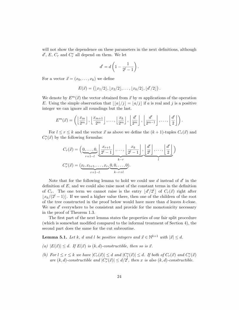
will not show the dependence on these parameters in the next definitions, althoughd′, E, Cr and C∗r all depend on them. We let

d′ = d

(1− 1

2l − 1

).

For a vector ~x = (x0, . . . , xk) we define

E(~x) =(bx1/2c, bx2/2c, . . . , bxk/2c, bd′/2c

).

We denote by Em(~x) the vector obtained from ~x by m applications of the operationE. Using the simple observation that bbac/jc = ba/jc if a is real and j is a positiveinteger we can ignore all roundings but the last.

Em(~x) =

(⌊xm2m

⌋,⌊xm+1

2m

⌋, . . . ,

⌊ xk2m

⌋,

⌊d′

2m

⌋,

⌊d′

2m−1

⌋, . . . ,

⌊d′

2

⌋).

For l ≤ r ≤ k and the vector ~x as above we define the (k + 1)-tuples Cr(~x) andC∗r (~x) by the following formulas:

Cr(~x) =(

0, . . . , 0,︸ ︷︷ ︸r+1−l

⌊xr+1

2l − 1

⌋, . . . ,

⌊xk

2l − 1

⌋,︸ ︷︷ ︸

k−r

⌊d′

2l

⌋, . . . ,

⌊d′

2

⌋︸ ︷︷ ︸

l

)

C∗r (~x) = (xl, xl+1, . . . , xr,︸ ︷︷ ︸r+1−l

0, 0, . . . , 0︸ ︷︷ ︸k−r+l

).

Note that for the following lemma to hold we could use d instead of d′ in thedefinition of E, and we could also raise most of the constant terms in the definitionof Cr. The one term we cannot raise is the entry bd′/2lc of Cr(~x) right afterbxk/(2l − 1)c. If we used a higher value there, then one of the children of the rootof the tree constructed in the proof below would have more than d leaves k-close.We use d′ everywhere to be consistent and provide for the monotonicity necessaryin the proof of Theorem 1.3.

The first part of the next lemma states the properties of our fair split procedure(which is somewhat modified compared to the informal treatment of Section 4), thesecond part does the same for the cut subroutine.

Lemma 5.1. Let k, d and l be positive integers and ~x ∈ Nk+1 with |~x| ≤ d.

(a) |E(~x)| ≤ d. If E(~x) is (k, d)-constructible, then so is ~x.

(b) For l ≤ r ≤ k we have |Cr(~x)| ≤ d and |C∗r (~x)| ≤ d. If both of Cr(~x) and C∗r (~x)are (k, d)-constructible and |C∗r (~x)| ≤ d/2l, then x is also (k, d)-constructible.

24

Proof. (a) We have |E(~x)| ≤ |~x|/2 + d′/2 < d. If there exists a (k, d, E(~x))-tree,take two disjoint copies of such a tree and connect them with a new root vertex,whose children are the roots of these trees. The new binary tree so obtained is a(k, d, ~x)-tree.

(b) The sum of the first k+1−l entries of Cr(~x) is at most |~x|/(2l−1) ≤ d/(2l−1),the remaining fixed terms sum to less than d′ = d(1 − 1/(2l − 1)), so |Cr(~x)| ≤ d.We trivially have |C∗r (~x)| ≤ |~x| ≤ d.

Let T be a (k, d, Cr(~x))-tree and T ∗ a (k, d, C∗r (~x))-tree. Consider a full binarytree of height l and attach T ∗ to one of the 2l leaves of this tree and attach a separatecopy of T to all remaining 2l − 1 leaves. This way we obtain a finite binary tree T ′.We claim that T ′ is a (k, d, ~x)-tree showing the constructibility of ~x and finishingthe proof of the lemma. To check condition (i) of the definition of a (k, d, ~x)-treenotice that no leaf of T ′ is in distance less than l from the root, leaves in distancel ≤ j ≤ r are all in T ∗ and leaves in distance r < j ≤ k are all in the 2l − 1 copiesof T . Hence(

0, . . . , 0, xl, . . . , xr, (2l − 1)

⌊xr+1

2l − 1

⌋, . . . , (2l − 1)

⌊xk

2l − 1

⌋)is a leaf-vector of the root of T ′, thus ~x is also a leaf-vector.

Condition (ii) is satisfied for the root, because it has at most |~x| ≤ d leaves thatare k-close. Notice that the nodes of T ′ of distance at least l from the root are alsonodes of T ∗ or a copy of T , so they satisfy condition (ii). There are two types ofvertices in distance 0 < j < l from the root. One of them has 2l−j copies of T belowit, the other has one less and also T ∗. In the first case we can bound the number ofk-close leaves by

2l−j(xr+1 + . . .+ xk

2l − 1+d′

2l+ . . .+

d′

2l−j+1

)≤ 2l−j

2l − 1· d+ d′

(1− 1

2j

)=

d

2l − 1

(2l−j + (2l − 2)

(1− 1

2j

))≤ d

2l − 1(2l − 1)

= d, (5.1)

where the last inequality holds since j ≥ 1. We also point out that here it is crucialthat we use the specific value of d′ < d.

In the second case, the number of k-close leaves is bounded by

(2l−j − 1)

(xr+1 + . . .+ xk

2l − 1+d′

2l+ . . .+

d′

2l−j+1

)+ |C∗r (~x)|

≤ (2l−j − 1)d

2l−j+d

2l≤ d,

where we used the result of the calculation in (5.1).

25

Armed with the last lemma we are ready to prove Theorem 1.3.

Proof of Theorem 1.3. We will show that (k, d)-trees exist for large enough k andd = b2k+1/(ek) + 100 · 2k+1/k3/2c.

We set l = blog(k)/2c, so 2l ∼√k. We will construct our vectors in such a way

that they start with 2l + 1 zeros.

We define the vectors ~x(t) = (x(t)0 , . . . , x

(t)k ) ∈ Nk+1 recursively. We start with

~x(0) = Ek−2l(~z), where ~z denotes the vector consisting of k + 1 zeros. For t ≥ 0we define ~x(t+1) = Ert−3l(Crt(~x

(t))), where rt is the smallest index in the range

3l ≤ rt ≤ k with∑rt

j=0 x(t)j /2

j ≥ 2−l. At this point we may consider the sequence

of the vectors ~x(t) end whenever the weight of one of them falls below 2−l and thusthe definition of rt does not make sense. But we will establish below that this neverhappens and the sequence is infinite.

Notice first, that for all t, the first 2l+1 entries of ~x(t) are zeros and all other en-tries are obtained from d′ by repeated application of dividing by an integer (namelyby 2l − 1 or by a power of 2) and taking lower integer part. As we have observedearlier in this section, we can ignore all roundings but the last. This way we can

write each of these entries in the form⌊

d′

2i(2l−1)c

⌋=⌊

d′

2i+lcαc⌋

for some non-negative

integers i and c and with α = 1 + 1/(2l − 1). We will use the values qt = rt − 2l(the length of the “left shift” when going from ~x(t) to ~x(t+1)) to give the exponentsof 2 and α explicitly for all 2l < j ≤ k and all t. We claim that

x(t)j =

⌊d′

2k+1−j αc(t,j)

⌋(5.2)

where c(t, j) is the largest integer 0 ≤ c ≤ t satisfying∑t−1

i=t−c qi ≤ k− j, c(0, j) = 0for all j, and c(t, j) = 0 if qt−1 > k − j.

The formal inductive proof of this formula becomes straightforward once weadopt the right perspective to keep track of how the entries develop during the

evolution of the vectors from ~x(0) to ~x(t). Namely, that each current entry x(t)j has

an “ancestor” that entered close to the right end of some vector ~x(t′) as x(t′)j′ =

bd′/2k+1−j′c and then got shifted to its current position as a result of applicationsof a certain number of Es and some Cris. As a first approximation we count adivision by 2 for each time the entry moved one place to the left — this explainsthe exponent k + 1 − j of the 2 in the formula. This is an accurate assumptionwhenever the left-shift was the result of an application of E. However when someCri was applied to an already existing entry, then the entry moved l places to theleft and the actual division was by 2l − 1 instead of 2l, so an extra factor of α hasto be included for correction. The exponent c(t, j) counts exactly how many suchα-factors are accumulated: this is exactly t− t′, that is, the number of Cri that were

applied to the ancestor of x(t)j after it got introduced into ~x(t′). Starting from the

26

rightmost entry, the entry must be shifted (k − j) places to the left and these areaccumulated via the left-shifts qt−1, . . . , qt′ , that are the result of the applicationsof Ert−1−3l ◦ Crt−1 , . . . E

r′t−3l ◦ Crt′ , respectively.

We claim next that c(t, j) and x(t)j increase monotonously in t for each fixed

2l < j ≤ k, while qt decreases monotonously in t. We prove these statements byinduction on t. We have c(0, j) = 0 for all j, so c(1, j) ≥ c(0, j). If c(t+1, j) ≥ c(t, j)for all j, then all entries of ~x(t+1) dominate the corresponding entries of x(t) by (5.2).

If x(t+1)j ≥ x(t)

j for all j, then we have rt+1 ≤ rt by the definition of these numbers,so we also have qt+1 ≤ qt. Finally, if q0 ≥ q1 ≥ · · · ≥ qt+1, then by the definition ofc(i, j) we have c(t+ 2, j) ≥ c(t+ 1, j).

The monotonicity just established also implies that the weight of ~x(t) is alsoincreasing, so if the weight of ~x(0) is at least 2−l, then so is the weight of all theother ~x(t), and thus the sequence is infinite. The weight of ~x(0) is

k∑j=2l+1

⌊d′

2k+1−j

⌋2j

>k∑

j=2l+1

d′

2k+1−j − 1

2j

> (k − 2l)d′

2k+1− 2−2l

> (k − log k)1− 1

2l−1

ek− 2− log k+2 −→ 1

e,

where the last inequality follows from d > 2k+1/(ek) and the last term tends to e−1

as k tends to infinity, so it is larger than 2−l for large enough k.We have just established that the sequence ~x(t) is infinite and coordinate-wise

increasing. Notice also that these vectors were obtained through the operations Eand Cr from the all-zero vector, so by Lemma 5.1 we must have |~x(t)| ≤ d for allt. Therefore the sequence ~x(t) must stabilize eventually. In fact, as the sequencestabilizes as soon as two consecutive vectors agree, it must stabilize in at most dsteps. So for some fixed vector ~x = (x0, . . . , xk) we have ~x(t) = ~x for all t ≥ d. Thisimplies that qt also stabilizes with qt = q for t ≥ d. Equation (5.2) as applied tot > d+ k simplifies to

xj =

⌊d′

2k+1−j αb(k−j)/qc

⌋. (5.3)

Recall that q = qt = rt − 2l (take t ≥ d), and rt is defined as the smallest indexin the range 3l ≤ r ≤ k with

∑rj=0 xj/2

j ≥ 2−l. Thus we have q ≥ l.

Proposition 5.2. We have q = l.

Proof. Assume for contradiction that q > l. Then by the minimality of rt we must

27

have

2−l >

2l+q−1∑j=0

xj2j

=

2l+q−1∑j=2l+1

⌊d′

2k+1−jαb(k−j)/qc

⌋2j

>

2l+q−1∑j=2l+1

d′

2k+1−jα(k−j)/q−1 − 1

2j

> (q − 1)d′

2k+1αk/q−4 − 2−2l.

In the last inequality we used jq ≤

2l+qq = 1 + 2l

q ≤ 1 + 2ll = 3. This inequality

simplifies to

2−l(1 + 2−l)α4 2k+1

d′> (q − 1)αk/q. (5.4)

We consider the problem of minimizing the right hand side over real numbers q > 2:Simple calculus gives that the corresponding value of q is sandwiched between q∗−1and q∗−2, where q∗ = q∗(k) = k lnα ∼

√k, and this minimum is more than (q∗−3)e.

Using α = 1 + 1/(2l − 1) > e2−lwe have q∗ ≥ k/2l. So (5.4) yields

2−l(1 + 2−l)α4 2k+1

d′>ke

2l− 3e.

Thus,

(1 + 2−l)α4 2k+1

d′− ke+ 3e2l > 0.

Substituting our choice for d, d′, α and l (as functions of k) and assuming that k islarge enough we get that the left hand side is at most(

1 +2√k

)(1 +

4√k

)4 2k+1

d(

1− 4√k

) − ek + 3e√k

≤(

1 +19√k

)ek(

1− 4√k

)(1 + 99e√

k

) − ek + 3e√k

≤(

1− 200√k

)ek − ek + 3e

√k = −200e

√k + 3e

√k < 0,

which is a contradiction. Hence q = l as claimed.

28

Having proved Proposition 5.2 we return to the proof of Theorem 1.3. Weestablish by downward induction that the vectors ~x(t) are constructible. We startwith t = d. Using (5.3) and the fact that q = l (Proposition 5.2) we get that forlarge k

w(~x(d)) ≥x

(d)2l+1

22l+1≥ d′

2k+1α

k−2l−1l−1 − 1

≥ d′

2k+1α

k2l − 1

≥ d/2

2k+1

(1 +

1√k

) klog k

− 1

≥ 1

2eke

k

2√k log k − 1 > 1.

So by Lemma 3.3, ~x(d) is constructible.Now assume that ~x(t+1) is constructible for some t ≤ d− 1. Recall that ~x(t+1) =

Ert−3l(Crt(~x(t))), so by (the repeated use of) part (a) of Lemma 5.1, Crt(~x

(t)) isconstructible. By part (b) of the same lemma, ~x(t) is also constructible (and thus theinductive step is complete) if we can (i) show that C∗rt(~x

(t)) is constructible and (ii)

establish that |C∗rt(~x(t))| ≤ d/2l. For (i) we use the definition of rt:

∑rtj=0 x

(t)j /2

j ≥2−l. But the weight of C∗rt(~x

(t)) is∑rt

j=l x(t)j /2

j−l, so the contribution of each term

with j ≥ l is multiplied by 2l, while the missing terms j < l contributed zeroanyway as the first 2l + 1 > l coordinates of x(t) are 0. This shows that the weightof C∗rt(~x

(t)) is at least 1 and therefore Lemma 3.3 proves (i).

For (ii) we use monotonicity to see |C∗rt(~x(t))| =

∑rtj=2l+1 x

(t)j ≤

∑rtj=2l+1 xj .

Here rt ≤ r0 ≤ k/2 for large enough k. Using the fact that q = l (Proposition 5.2)and (5.3) we further have for large k that

|C∗rt(~x(t))| ≤ d′

rt∑j=2l+1

1

2k+1−j · αk−jl

≤ d

rt∑j=2l+1

(α2

)k−j≤ d

(3

4

)k−rt· 4

(since

α

2≤ 3

4

)≤ d

(3

4

) k2

· 4(

since rt ≤k

2

)<

d√k≤ d

2l.

29

This finishes the proof of (ii) and hence the inductive proof that ~x(t) is constructiblefor every t.

As ~x(0) = Ek−2l(~z) is constructible, Lemma 5.1 (a) implies that the all-zerovector ~z is also constructible. Thus the larger vector (0, . . . , 0, d) is constructibletoo, and by Observation 3.1 there exists a (k, d)-tree.

6 Proof of the Lower Bound of Theorem 1.1

Let us first give the intuition of where the factor two improvement is coming fromcompared to using just the classical Local Lemma (c.f. (1.2)) and what is the reasonbehind the counterintuitive probabilities we use to choose the assignment.

When using the classical Local Lemma to give a lower bound on f(k), one sets

each variable independently to true or false uniformly at random and the⌊

2k

ek

⌋lower bound in (1.2) is immediate. However in the proof we must consider all pairsof clauses sharing a variable as “dependent on each other”. The lopsided versionof the Local Lemma [11] allows for a more restricted definition of “intersecting”clauses. Namely, one can consider two clauses intersect only if they contain a com-mon variable with different sign and this still allows for the same conclusion as inthe classical Local Lemma. If all variables in a (k, s)-CNF are balanced, that is theyappear an equal number of times with either sign, then each clause intersects onlyat most ks/2 other clauses in this restricted sense, instead of the at most k(s − 1)other clauses it may intersect in the original sense and the factor two improvementis immediate. To handle the unbalanced case we consider a distribution on assign-ments where the variables are assigned true or false values with some bias. Itwould be natural to favor the assignment that satisfies more clauses, but the oppo-site turns out to be the distribution that works. This is because the clauses withmany variables receiving the less frequent sign are those that intersect more thanthe average number of other clauses, so for the use of the Lopsided Local Lemmathose are the ones whose satisfiability should be boosted with the bias put on theassignments.

Proof of lower bound in Theorem 1.1. Let F be a (k, s)-CNF formula with s =⌊2k+1

e(k+1)

⌋.

For a literal v we denote by dv the number of occurrences of v in F . We set avariable x to true with probability Px = 1

2 + 2dx−s2sk . This makes the negated version

x satisfied with probability Px = 12 −

2dx−s2sk ≥

12 + 2dx−s

2sk as we have dx + dx ≤ s. So

any literal v is satisfied with probability at least 12 + 2dv−s

2sk .In order to prove that the formula F is satisfied with non-zero probability we

need the Lopsided Local Lemma of Erdos and Spencer.

30

Lemma 6.1 ([11]). Let {AC}C∈I be a finite set of events in some probability space.Let Γ(C) be a subset of I for each C ∈ I such that for every subset J ⊆ I \ (Γ(C)∪{C}) we have

Pr(AC | ∧D∈J AD) ≤ Pr(AC).

Suppose there are real numbers 0 < xC < 1 for C ∈ I such that for every C ∈ I wehave

Pr(AC) ≤ xC∏

D∈Γ(C)

(1− xD).

ThenPr(∧C∈IAC) > 0.

For each clause C in F , we define the “bad event” AC to be that C is notsatisfied. Moreover, for every C in F we define Γ(C) to be the family of clauses Din F that have at least one such variable in common with C whose sign is differentin C and D. Finally, we set the value of each xC to be x = e

2k.

We need to check that for every subset J ⊆ I \ (Γ(C) ∪ {C}) we have

Pr(AC | ∧D∈J AD) ≤ Pr(AC).

This is equivalent to Pr(∧D∈J AD|AC) ≤ Pr(∧D∈J AD). The right hand side issimply the probability of a random assignment satisfying all clauses in J . The lefthand side can be interpreted as the same probability after a random assignment ismodified by setting all literals in C to false. The random assignment does notsatisfy any clauses in J after the modification that it did not satisfy before, since noclause from J contains a variable of C in the opposite form. Hence the probabilityof satisfying all of them does not grow by the modification proving the inequality.(The probability might, in fact, decrease if some of the clauses in J contain a literalalso present in C.)

We need to check also the other condition of the lemma. Let C be an arbitraryclause and let us denote the literals it contains by v1, . . . , vk. For C not to besatisfied we must not set any of the independent literals in C to true, and therefore

31

we have

Pr(AC) =k∏i=1

(1− Pvi)

≤k∏i=1

(1

2− 2dvi − s

2sk

)

≤ 1

2k

k∏i=1

((1 +

1

k

)(1− edvi

2k

))

≤(1 + 1

k

)k2k

k∏i=1

(1− x)dvi

<e

2k(1− x)|Γ(C)|

= x∏

D∈Γ(C)

(1− x).

The inequality in the fourth line holds due to the well-known inequality that 1−ax ≤(1− x)a for every 0 < x < 1 and a ≥ 1.

As the conditions of the Lopsided Local Lemma are satisfied, its conclusion mustalso hold. It states that the random evaluation of the variables we consider satisfiesthe (k, s)-CNF F with positive probability. Thus F must be satisfiable and we have

f(k) ≥ s =⌊

2k+1

e(k+1)

⌋.

7 More About the Class MU(1) and the NeighborhoodConjecture

7.1 Constructing binary trees and MU(1) formulas

The structure of MU(1) formulas is well understood and it is closely related tobinary trees. (Recall that by a binary tree we always mean a rooted tree whereevery non-leaf node has exactly two children.) In particular, given any binarytree T , we associate with it certain CNF formulas. Similarly to Section 2.1 westart with assigning distinct literals to the vertices, assigning the negated and non-negated form of the same variable to the two children of any non-leaf vertex. Wedo not assign any literal to the root. For each leaf of T select a clause that is thedisjunction of some literals along the path from the root to that leaf and considerthe CNF formula F that is the conjunction of one clause for each leaf. Clearly, Fis unsatisfiable and it has one more clause than the number of variables associated

32

with T . Note that for proving the upper bound in Theorem 1.1 we used (k, d)-treesT and the associated unsatisfiable (cf. Observation 2.1) (k, d)-CNF Fk(T ) that wasconstructed similarly, but selecting the k vertices farthest from the root on everyroot-leaf path.

As proved in [7], F is a MU(1) formula if and only if all literals associated tovertices of T do appear in F , furthermore every formula in MU(1) can be obtainedfrom a suitable binary tree this way.

Recall that ftree(k) denotes the smallest integer d such that a (k, d)-tree exists.Clearly, f(k) ≤ f1(k) < ftree(k), and we showed that f(k) = (1 + o(1))ftree(k).

7.2 On the size of unsatisfiable formulas

By the size of a rooted tree we mean the number of its leaves and by the size ofa CNF formula we mean the number of its clauses. With this notation the size ofa containment-minimal (k, d)-tree T and the size of the corresponding (k, d)-CNFFk(T ) in MU(1) are the same.

When proving the upper bound of Theorem 1.1 we constructed (k, d)-trees for

d ≈ 2k+1

ek . Their size and therefore the size of the corresponding (k, d)-CNF inMU(1) is at most 2h, where h is the height of the tree. In fact, the sizes of the treeswe constructed are very close to this upper bound. Therefore it makes sense to takea closer look at the height.

Recall that we associated with a vertex v of a (k, d)-tree the vector (x0, . . . , xk),where xj is the number of leaf-descendants of v of distance j from v. If a (k, d)-tree has minimal size it has no two vertices along the same branch with identicalvectors. In fact, this statement is also true even if one forgets about the last entryin the vector. So the minimal height of a (k, d)-tree is limited by the number ofvectors in Nk with L1 norm at most d, which is

(d+kk

)≤ dk. For d = ftree(k) this

is 2O(k2). For the minimal size of a (k, d)-tree this implies a 22O(k2)bound that

applies whenever such a tree exists. The same bound for minimal size (k, d)-CNFformulas in MU(1) is implicit in [18]. There is numerical evidence that the sizes ofthe minimal (k, ftree(k))-tree and the minimal (k, f1(k) + 1)-CNF in MU(1) mightindeed be doubly exponential in k (consider the size of the minimal (7, 18)-tree andthe minimal (7, 18)-CNF in MU(1) mentioned below).

A closer analysis of the proof of the upper bound in Theorem 1.3 shows that theheight of the (k, d)-tree constructed there is at most d log k. While this is betterthan the general upper bound above it still allows for trees with sizes that are doublyexponential in k.

This height can, however, be substantially decreased if we allow the error termin d to slightly grow. If we allow d = (1 + ε)2k+1

ek for a fixed ε > 0, then a morecareful analysis shows that the height of the tree created becomes Oε(k). Thismeans that the size of the tree and the corresponding formula is bounded by a

33

polynomial in d. Here we just sketch an informal argument for this statement,using the continuous approach of Section 4. We briefly recall and follow throughthe idea of Subsection 4.2, keeping track of the height of the constructed tree andneglecting the same small error terms neglected there. Our choice of d translatesto the setting of the parameter T = e

1+ε there. We build a (k, d)-tree startingfrom a full binary tree of depth k. (In fact the true depth is k − o(k), but weneglect this difference too.) We associate vectors of length k + 1 (the leaf-vectors)with the vertices. In the process we ignore the leaves whose leaf-vectors satisfythe conditions of Lemma 3.3, as they are constructible. At any given step of theconstruction all other leaves share the same leaf-vector and their distance fromthe root is the depth of the current tree. At the next step we attach new treesto the non-ignored leaves and thereby increase the depth of the current tree. Weapproximate the development of the leaf-vectors of the leaves with a two variablefunction F (t, x), where t refers to “time” and, in fact, corresponds to the depthof the current tree (not counting the depth of the initial full binary tree). Moreprecisely, the jth term of the leaf-vector of vertices in depth m > k is approximated

by F(mk − 1, jk

)d

2k+1−j . In Subsection 4.2 we develop a differential equation for F

and by studying it, we show that∫ 1

0 F (t, x) dx > T is satisfied for some value of tdepending only on T < e (and, through T , depending on ε). This means that theleaf-vectors at distance tk+k from the root satisfy the conditions of Lemma 3.3. Westop this process at this depth and obtain a binary tree with all its leaves satisfyingthe requirements of the lemma. This tree is still incomplete, but the construction ofthe (k, d)-tree can be completed with attaching suitable binary trees to all the leavesof this incomplete tree. The existence of suitable trees is guaranteed by Lemma 3.3and the simple proof of the lemma shows that these trees can be chosen to havedepth at most k. This concludes the argument, which then can be made formalusing a discretization analogous to the one in Section 5.

Let us define f1(k, d) for d > f1(k) to be the minimal size of a (k, d)-CNFin MU(1), and let ftree(k, d) stand for the minimal size of a (k, d)-tree, assumingd ≥ ftree(k). While f1(k, f1(k) + 1) and similarly ftree(k, ftree(k))) are probablydoubly exponential in k, the above argument shows that for slightly larger valuesof d = (1 + ε)f(k) the values ftree(k, d) and hence also f1(k, d) are polynomial in d(and thus simply exponential in k).

7.3 Extremal Values and Algorithms

Finally, we mention the question whether ftree(k) = f1(k) + 1 for all k. (The+1 term comes from us defining these functions inconsistently. While f(k) andf1(k) is traditionally defined as the largest value d with all (k, d)-CNF satisfiable orno (k, d)-CNF in MU(1) exist, respectively, it was more convenient for us to defineftree(k) as the smallest value d for which (k, d)-trees exist.) This question asks if one

34

necessarily loses (in the maximal number of appearances of a variable) by selectingthe k vertices farthest from the root when making an MU(1) k-CNF formula from abinary tree. As mentioned above, f(k) = f1(k) is also open, but ftree(k) = f1(k) +1 seems to be a simpler question as both functions are computable. Computingtheir values up to k = 8 we found these values agreed. To gain more insight wecomputed the corresponding size functions too and found that ftree(k, d) = f1(k, d)for k ≤ 7 and all d > f1(k) with just a single exception. We have f1(7) = 17and f1(7, 18) = 10, 197, 246, 480, 846 < ftree(7, 18) = 10, 262, 519, 933, 858. We alsofound f1(8, d) = ftree(8, d) for f1(8) = 29 < d ≤ 33. Is f1(7, 18) < ftree(7, 18) theexception or will it turn into the rule for larger values? Does it indicate that ftree(k)and f1(k) + 1 will eventually diverge?

A related algorithmic question is whether the somewhat simpler structure of(k, d)-trees can be used to find an algorithm computing ftree(k) substantially fasterthan the algorithm of Hoory and Szeider [18] for computing f1(k). Such an algorithmwould give useful estimates for f1(k) and also f(k). At present we use a similar(and similarly slow) algorithm for either function.

7.4 Pairing strategies and the Neighborhood Conjecture

Determining whether the Local Lemma 2-coloring bounds in (1.4) and (1.5) have anygame-theoretic generalizations is still open. To formalize this problem we introduce

D(k) := min{d : ∃ k-uniform Maker’s win F with ∆(F) = d}

as the critical maximum degree for the Neighborhood Conjecture. By definition,every k-uniform F with ∆(F) ≤ D(k)−1 is Breaker’s win and hence it is 2-colorableby (1.3).

In [3] various weaker versions of the original Neighborhood Conjecture are stated,maybe the most fundamental one is whether D(k) grows exponentially:

Problem 7.1. Does there exist an ε > 0 such that D(k) > (1 + ε)k holds for all k?

Theorem 1.6 provides an upper bound for D(k). For the proof of this theoremwe constructed a k-uniform hypergraph with bounded maximum degree and gaveMaker a winning strategy based on a pairing of the vertices. The point we would liketo make in this section is that in order to approach the Neighborhood Conjectureany closer, the study of these kind of pairing strategies is insufficient in eitherdirection: we must develop methods that are able to tackle non-pairing strategies.

We call a strategy for either player in the Maker-Breaker game a pairing strategyif it is defined by a partition of a subset of the vertex set into pairs and calls forthe player to respond with claiming the pair of the vertex last claimed by heropponent. (In case the opponent claimed an unpaired vertex or a vertex whose pairis already claimed, the move is arbitrary.) In addition, a pairing strategy for Maker

35

also specifies a starting vertex, disjoint from the pairs, to be claimed first. Notethat a player playing by a pairing strategy is guaranteed to eventually claim at leastone member of every pair. We call a hypergraph PairingBreaker’s win (respectively,PairingMaker’s win) if Breaker (respectively, Maker) has a winning pairing strategy.

Equivalently, we call a hypergraph (V,F) a PairingBreaker’s win, if there existsa partition of a subset V ′ = ∪Xi ⊆ V into disjoint subsets Xi of size two, suchthat for every F ∈ F there exists an index i with Xi ⊆ F . The hypergraph isa PairingMaker’s win, if there exists a vertex x0 ∈ V and a partition of a subsetV ′ = ∪Xi ⊆ V \ {x0} into disjoint subsets Xi of size two, such that for every subsetM , x0 ∈ M ⊆ V , with |M ∩ Xi| ≥ 1 for every i, there exists an F ∈ F withF ⊆ M . To see the equivalence note that for partitions that leave out at most asingle element of V , the corresponding pairing strategy is winning if and only if theabove combinatorial condition is satisfied.

Analogously for D(k), we define

Dpairing(k) := min{d : ∃ k-uniform PairingMaker’s win F with ∆(F) = d},D∗pairing(k) := min{d : ∃ k-uniform F with ∆(F) = d, not PairingBreaker’s win}.

Requiring a player to play a pairing strategy is a restriction, so we have:

D∗pairing(k) ≤ D(k) ≤ Dpairing(k). (7.1)

It is interesting to note that both the functions D∗pairing and Dpairing are wellunderstood, but D is not. The above inequalities are the only known bounds forD(k).

The value of D∗pairing(k) can be easily concluded from the classic observation ofHales and Jewett [17] connecting Hall’s Theorem to pairing strategies (cf. [3]). Weindicate the simple proof to be self-contained.

Proposition 7.2. For every k we have D∗pairing(k) = bk/2c+ 1.

Proof. For the lower bound let us assume first that F is a k-uniform hypergraph withd := ∆(F) ≤ k/2. By Hall’s theorem we can select two representatives xF , yF ∈ Ffor every edge F ∈ F such that all these 2|F| elements are distinct. These pairsprovide Breaker with a winning pairing strategy, since he can occupy one vertexfrom each element of F .

For the upper bound let us consider any k-uniform d-regular hypergraph (V,F)with no two hyperedges sharing more than a single vertex. One can, for example,take the vertex set V = {1, . . . , k}d to be the d-dimensional grid, and the family Fconsisting of all its subsets on axis parallel lines. We show D∗pairing(k) ≤ bk/2c+1 byshowing that the hypergraph (V,F) is not PairingBreaker’s win if d > k/2. Indeed,if Breaker had a winning pairing strategy, then there is a family of disjoint pairssuch that all hyperedges F ∈ F contain one of these pairs. These pairs must be

36

distinct for different hyperedges as two hyperedges of F do not share two vertices.But then we have |V |/2 ≥ |F| and therefore k/d = |V |/|F| ≥ 2, providing acontradiction.

Our results in this paper determine Dpairing(k) asymptotically.

Theorem 7.3. For every k ≥ 3 we have

f(k)/2 < Dpairing(k) ≤ 2ftree(k − 2).

In particular, we have

Dpairing(k) =2k

ek(1 + o(1)).

Proof. The upper bound follows from part (i) of Theorem 1.6 as the winning strat-egy we construct there for Maker is, in fact, a pairing strategy. Actually, the slightlystronger bound Dpairing(k) ≤ ftree(k−1) can also be proved with the same argument.

For the lower bound we construct an unsatisfiable (k, 2∆(H))-CNF formulaF (H) from a PairingMaker’s win hypergraph (V,H).

First we create a new hypergraph F by taking two disjoint copies of H anddefine a partition of its vertex set into pairs by keeping the pairs from the pairingstrategy in both copies and adding a last pair consisting of the starting vertices inthe two copies. Then, for each pair Yi in our partition ∪Yi ⊆ V (F) we introduce avariable vi and label one of the vertices in Yi with vi and the other with vi. For therest of the vertices, from V (F)\∪Yi, we introduce a separate new variable for each.We construct a clause C(F ) from each hyperedge F ∈ F by taking the disjunctionof the labels of the vertices. Finally F (H) is the conjunction of the clauses C(F )for F ∈ F . Note that each variable appears at most 2∆(H) times in F (H).

Consider now any assignment α to this formula. We want to prove that α isnot a satisfying assignment. Let us consider the set S of vertices of F whose labelin α evaluates to false. Then S contains the starting vertex of exactly one of thecopies H1 of H, as well as one vertex from each pair in this copy. Since the pairingdefines a winning strategy for Maker in H1 there exists a set F ∈ H1 such thatF ⊆ S. Each literal of the corresponding clause C(F ) evaluates to false, so α isnot satisfying.

Finally, the asymptotic statement follows from our lower and upper bounds, andTheorems 1.1 and 1.3, respectively.

The gap between the lower and upper bounds forD(k) in Inequality (7.1) is huge.To make it any smaller, by the above, one must consider non-pairing strategies. Eventhe following problem is open:

Problem 7.4. Does D(k) = D∗pairing(k) = bk/2c+ 1 hold for every k?

37

The equality above holds for k ≤ 4 as the hypergraph dual of the Petersengraph is a Maker’s win 3-uniform hypergraph of maximum degree 2 and Knox [21]constructed 4-uniform Maker’s win hypergraphs with maximum degree 3. HoweverProblem 7.4 is open for every k > 4. It seems likely that resolving it in eitherdirection will require a new idea and hence might lead to a more significant progresson the Neighborhood Conjecture itself.

A more modest problem is to try to separate D(k) from Dpairing(k). We knowthat D(2) = 2 = Dpairing(k), as shown by a triangle. What happens for k = 3?We of course know that the hypergraph dual of the Petersen graph is a 3-uniformMaker’s win hypergraph with maximum degree 2, but does there exists a 3-uniformhypergraph with maximum degree 2 which is a PairingMaker’s win?

Problem 7.5. Prove that for all large enough k we have D(k) < Dpairing(k).

Acknowledgment: We would like to thank the referees for their many insight-ful comments.

References

[1] R. Aharoni and N. Linial, Minimal non-two-colorable hypergraphs and minimalunsatisfiable formulas, J. Combin. Theory Ser. A 43, (1986), 196–204.

[2] N. Alon, J. Spencer, The Probabilistic Method, John Wiley-Interscience, 2008.

[3] J. Beck, Combinatorial Games: Tic Tac Toe Theory, Encyclopedia of Mathe-matics and Its Applications 114, 2008

[4] P. Berman and M. Karpinski, On Some Tighter Inapproximability ResultsProc. 26th ICALP (1999), LNCS 1644, Springer 1999, 200-209.

[5] P. Berman, M. Karpinski, and A. D. Scott, Approximation hardness and sat-isfiability of bounded occurrence instances of SAT. Electronic Colloquium onComputational Complexity (ECCC), 10 (022), 2003.

[6] S.A. Cook, The complexity of theorem-proving procedures, Proc. 3rd Ann.ACM Symp. on Theory of Computing (STOC) (1971), 151–158.

[7] G. Davydov, I. Davydova, and H. Kleine Buning, An efficient algorithm forthe minimal unsatisfiability problem for a subclass of CNF, Artif. Intell. 23,(1998), 229–245.

[8] B. Doerr, Vector Balancing Games with Aging, Journal of Combinatorial The-ory, Series A 95 (2001), 219–233.

38

[9] B. Doerr, European Tenure Games, Theoretical Computer Science 313 (2004),339–351.

[10] O. Dubois, On the r, s-SAT satisfiability problem and a conjecture of Tovey,Discrete Appl. Math. 26 (1990), 51-60.

[11] P. Erdos and J.Spencer, Lopsided Lovasz Local Lemma and Latin transversalsDiscrete Appl. Math. 30, (1991), 151–154.

[12] P. Erdos and J.L. Selfridge, On a combinatorial game, J. Combinatorial TheorySer. A 14, (1973), 298–301.

[13] U. Feige, A threshold of lnn for approximating set cover, J. ACM 45(4), (1998),634–652.

[14] C.M. Fortuin, P.N. Kasteleyn, J. Ginibre, Correlation inequalities for somepartially ordered sets, Comm. Math. Phys. 22 (1971), 89–103

[15] H. Gebauer, R. A. Moser, D. Scheder and E. Welzl, The Lovasz Local Lemmaand Satisfiability Efficient Algorithms, (2009), 30–54.

[16] H. Gebauer, Disproof of the Neighborhood Conjecture with Implications toSAT, Combinatorica 32(5), (2012), 573–587.

[17] A. W. Hales, R. I. Jewett, Regularity and positional games, Trans. Amer.Math. Soc. 106 (1963), 222–229

[18] S. Hoory and S. Szeider. Computing unsatisfiable k-SAT instances with fewoccurrences per variable, Theoretical Computer Science 337(1–3) (2005), 347–359.

[19] S. Hoory and S. Szeider, A note on unsatisfiable k-CNF formulas with fewoccurrences per variable, SIAM J. Discrete Math 20 (2), (2006), 523–528.

[20] H. Kleine Buning and X. Zhao, On the structure of some classes of minimalunsatisfiable formulas, Discr. Appl. Math. 130(2), (2003), 185–207.

[21] Fiachra Knox, Two constructions relating to conjectures of Beck on positionalgames, http://arxiv.org/pdf/1212.3345v1.pdf.

[22] L. G. Kraft, A device for quantizing, grouping, coding amplitude modulatedpulses, M.S. thesis, Electrical Engineering Department, MIT (1949).

[23] J. Kratochvıl, P. Savicky and Z. Tuza, One more occurrence of variables makessatisfiability jump from trivial to NP-complete, SIAM J. Comput. 22 (1),(1993), 203–210.

39

[24] O. Kullmann, An application of matroid theory to the SAT problem, FifteenthAnnual IEEE Conference on Computational Complexity (2000), 116-124

[25] R.A. Moser, G. Tardos, A Constructive Proof of the General Lovasz LocalLemma, J. ACM 57(2), (2010)

[26] A. Pelc, Searching games with errors—fifty years of coping with liars TheoreticalComputer Science 270 (1–2) (2002), 71–109.

[27] http://polymathprojects.org/2012/07/12/minipolymath4-project-imo-2012-q3/

[28] C.H. Papadimitriou and M. Yannakakis, Optimization, approximation, andcomplexity classes, J. Comput. System Sci. 43 (3), (1991), 425–440

[29] J. Radhakrishnan, A. Srinivasan, Improved bounds and algorithms for hyper-graph 2-coloring, Random Structures Algorithms 16 (3), (2000), 4–32

[30] S. Roman, Coding and Information Theory, Springer, New York (1992).

[31] P. Savicky and J. Sgall, DNF tautologies with a limited number of occurrencesof every variable, Theoret. Comput. Sci. 238 (1–2), (2000), 495–498.

[32] D. Scheder, Unsatisfiable Linear CNF Formulas Are Large and Complex, 27thInternational Symposium on Theoretical Aspects of Computer Science (STACS)(2010), 621–631

[33] J.B. Shearer, On a problem of Spencer, Combinatorica 5, (1985), 241–245

[34] J. Spencer, Randomization, Derandomization and Antiderandomization: ThreeGames, Theoretical Computer Science 131 (1994), 415–429.

[35] S. Szeider, Homomorphisms of conjunctive normal forms, Discr. Appl. Math.130(2), (2003), 351–365

[36] C.A. Tovey, A simplified NP-complete satisfiability problem, Discr. Appl.Math. 8 (1), (1984), 85–89.

40