the location - routing problem of electric vehicles in
TRANSCRIPT

POLITECNICO DI TORINO
Department of Mechanical and Aerospace Engineering
Master Degree
In Automotive Engineering
Master Thesis
The Location - Routing Problem of Electric Vehicles in City
Logistics
Supervisor
Prof. Eugenio Morello
Prof. Massimo Simone
Prof. Alessandro Leverano
Candidate
Shangguan Tong
14th October 2020
Table of Contents 0. Abstract .................................................................................................................................................................................... 1
1. Introductions to the related theories ............................................................................................................................. 2
1.1 City logistics ................................................................................................................................................................. 2
1.1.1 Last mile delivery........................................................................................................................................... 2
1.2 Green logistics ............................................................................................................................................................ 3
1.2.1 Low-carbon logistics ................................................................................................................................... 4
1.2.2 Carbon emissions cost calculation .......................................................................................................... 5
1.3 Incentive policies and measures ........................................................................................................................... 7
2. Electric vehicles applications in city logistics................................................................................................................ 8
2.1 Relevant concepts ..................................................................................................................................................... 8
2.1.1 Types of electric vehicles ............................................................................................................................ 8
2.1.2 Characteristics of Electric vehicles ........................................................................................................... 9
2.1.3 Charging modes and charging infrastructures ................................................................................. 10
2.2 Application status .................................................................................................................................................... 11
3. Vehicle distribution system relevant concepts .......................................................................................................... 14
3.1 Location allocation problem (LAP) .................................................................................................................... 14
3.2 Vehicle routing problem ....................................................................................................................................... 17
3.3 Location-Routing problem .................................................................................................................................. 19
4. Location-routing problem of electric vehicles model formulation .................................................................... 21
4.1 Model description ................................................................................................................................................... 21
4.2 Assumptions and notations of model .............................................................................................................. 22
4.3 Build the model ........................................................................................................................................................ 24
4.3.1 Determine the objective functions ........................................................................................................ 24
4.3.2 Mathematical model .................................................................................................................................. 26
5.Algorithm design for electric vehicle location-routing problem ......................................................................... 29
5.1 Algorithm overview ................................................................................................................................................. 29
5.1.1 Exact algorithms .......................................................................................................................................... 29
5.1.2 Heuristics algorithms ................................................................................................................................. 30
5.1.3 Metaheuristics .............................................................................................................................................. 31
5.2 Genetic algorithm overview ................................................................................................................................. 33
5.2.1 Introduction .................................................................................................................................................. 33
5.2.2 Basic process ................................................................................................................................................ 34
5.2.3 Determine the parameters....................................................................................................................... 36
5.2.4 Advantages and disadvantages of genetic algorithm .................................................................... 37
5.3 Algorithm process design ..................................................................................................................................... 37
5.3.1 Chromosome coding and decoding .................................................................................................... 37
5.3.2 Generate initial population ...................................................................................................................... 39
5.3.3 Fitness function ............................................................................................................................................ 40
5.3.4 Genetic operators ....................................................................................................................................... 40
6. Case analysis ......................................................................................................................................................................... 46
6.1 Algorithm implementation ................................................................................................................................... 46
6.2 Basic data ................................................................................................................................................................... 47
6.2.1 Charging station .......................................................................................................................................... 47
6.2.2 Vehicle relevant parameters .................................................................................................................... 48

6.3 Result analysis ........................................................................................................................................................... 50
6.2.1 medium-scale case result analysis ........................................................................................................ 50
6.2.2 large-scale case result analysis .............................................................................................................. 54
6.4 Conclusions ............................................................................................................................................................... 58
REFERENCES .............................................................................................................................................................................. 61
APPENDIX ................................................................................................................................................................................... 63

1
0. Abstract
Recent years, with the rapid development of transportation and the increasing number of vehicles, motor
vehicles have become an important source of urban environmental pollution and traffic congestion problems.
Currently, 25% of CO2 come from transportation industry (Dablanc,2011). In response of side effects of the
transportation sector on energy and the environment, many countries have adopted the development of new
energy vehicles as a national strategy. As a representative of new energy vehicles, electric vehicles (EVs) with
zero pollution and low energy consumption have been rapidly developed, it is also imperative to popularize EVs
in the logistic sector, benefits from reducing harmful gas emissions and logistics costs.
Compared with the traditional fuel vehicles, the EVs distribution faces some difficulties such as battery
capacity limitations, long charging time and few charging facilities. At present, the difficulty of charging
seriously restricts the marketing promotion of EVs. Consummating the deployment of charging facilities are an
important guarantee for the extensive use of EVs. The rational layout of charging stations is particularly
important. The traditional vehicle routing problem cannot be directly applied to the EVs distribution system. The
charging station location problem and the routing problem of EVs are interdependent.
This thesis mainly discusses:
⚫ The problem of using EVs in logistics industry, especially in urban last mile delivery.
⚫ Based on Genetic algorithm, design a model for solving optimization problems for both Charging Station
Location Allocation Problem (CS-LAP) and for Electric Vehicle Routing Problem (E-VRP).
⚫ Analyze some examples of scenario, compare the logistics costs between traditional vehicles and EVs.
2
1. Introductions to the related theories
1.1 City logistics
City logistics (urban freight distribution) generally is the logistic companies provide a series of logistics
services to the customer points that distributed in urban area, these services includes processing, packaging,
loading and unloading, distribution, etc. City logistics is an important activity that connects the exchange of
goods between the city and the outside. It has a linking role in the entire logistics distribution system.
Mainly have the following contents and characteristics [1][2][3]:
1) The distribution area is relatively concentrated and fixed. The area is often bounded by the entire city
boundary. So, it has the remarkable characteristic of short distribution distance.
2) The scale of urban logistics is huge. Urban logistics mainly occurs in densely populated and resource-
intensive urban areas, so the customers’ needs are various and huge amounts. The common distribution
forms are small-batch and multi-frequency.
3) Urban logistics pay attention to customer service quality. It is directly facing to customers, so the quality of
service directly affects the corporate image and reputation of company. Service quality is mainly embodied
in whether the product packaging is intact, whether the delivery is on time, etc.
4) The vehicle speed is not high. In urban logistics, because the city traffic conditions are complicated, such
as traffic congestion and road maintenance. Besides, under the control of traffic lights, the speed of
distribution vehicles cannot be very high.
5) Low requirements for vehicle power performance. Due to the low speed restricted by urban roads, the
requirements for vehicle power performance are generally low. Therefore, urban logistics companies pay
more attention to the cargo loading capacity and operating costs when choosing the means of transport.
1.1.1 Last mile delivery
Delivery is the process of transporting goods from a source location to a predefined destination. The general
process of delivering goods is known as distribution. Last mile delivery describes the movement of people and
goods from a transportation hub to a final destination, it is the terminal distribution of urban freight distribution
[4]. As a special type of distribution, last mile service provides short-distance and point-to-point distribution
within cities, it can be divided into professional distribution and general merchandise distribution, as shown in

3
Figure 1.1:
Figure 1.1 Last mile delivery classification
Professional distribution: the main customers are small and medium-sized enterprises and large supermarkets
in the city. General merchandise distribution: this type of demands has a wide variety, high timeliness
requirements, high distribution frequency and uneven distribution, the main customers are small enterprises,
residents and individuals.
The distribution mode consists of four types [5]:
1) Self-delivery mode (direct delivery by suppliers);
2) Collaborative delivery mode (a number of logistics enterprises cooperated in a certain distribution area);
3) Outsourced delivery mode (the third-party logistics);
4) Integrated delivery mode (from production to transportation process comprehensively distribute goods by
enterprises).
With the development of cities and the transformation of resident’s consumption patterns, cities need more
efficient distribution systems to support the daily operation of cities. At the same time, residents’ higher pursuit
of the urban living environment also requires logistics activities to reduce their negative impacts on environment
and reduce energy consumption. Logistics is a key industry of the national economy, in China, logistic costs
relative to GDP accounted for 14.6% in the first half of 2019 [6], and itself is also a major energy consumer and
high emissions, so “Greening” logistic industry is imperative.
1.2 Green logistics
Green logistics refers to the use of advanced logistics technology to plan and implement logistics activities to
restrain harm to environments and reduce resource consumption. The ultimate goal of green logistic is to
minimize the impact of logistics activities on the environment and achieve sustainable development.
The significance of developing green logistics is not only in energy saving and emission reduction, for
logistics companies, it can also reduce logistics costs and improve economic and social benefits. The
4
development of green logistics is not only to achieve greening through technical means and management in a
certain part of logistics. Moreover, the operation is carried out through all links in the logistics to realize the
greening of the entire logistics system.
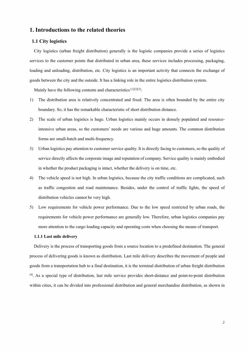
Green logistics is developed on the basis of traditional logistics, in term of operation process it is similar to
traditional logistics. To realize a green logistics system, it is necessary to realize the greening of packaging,
handling, transportation, storage, distribution, waste treatment, etc. Figure 1.2 shows the green logistics structure
diagram [1]:
Figure 1.2 green logistic structure diagram
1.2.1 Low-carbon logistics
Green logistics is a concept with deep meaning, all methods and processes aimed at reducing the ecological
environment impact during logistics process belong to the category of green logistics. While, low-carbon
logistics emphasizes environmental protection, which can reduce the carbon intensity (the ratio of greenhouse
gas emissions produced to GDP) during logistics. In terms of scope, green logistics includes low-carbon logistics,
green logistics is richer in connotation [7].
The origin of low-carbon logistics is attributed to the low-carbon economy and the Copenhagen Environment
Conference’s advocacy of green issues. Low-carbon economy means that under the guidance of the concept of
sustainable development, through technological innovation, institutional innovation, industrial transformation,
new energy development and other means, as much as possible to reduce the consumption of high-carbon energy
such as coal and petroleum, reduce greenhouse gas emissions, and achieve a win-win economic development
pattern for social development and ecological environment protection.
Often most of the logistics cost lies in the transportation goods, and the carbon emissions caused by vehicle

5
transportation also account for a large proportion of the carbon emissions of the entire logistics system.
1.2.2 Carbon emissions cost calculation
Carbon emission is an abbreviation for greenhouse gas emission, which is proposed under the background of
global warming. Greenhous gases mainly include carbon dioxide (CO2), methane (CH4), nitrous oxide (N2O),
ozone (O3), chlorofluorocarbons (CFCS), etc. The largest proportion is CO2 among greenhouse gases [8].
Therefore, “Carbon” is used to represent greenhouse gas emissions. In this thesis, we mainly discuss the carbon
dioxide gas, other gases are not considered due to small proportions. Because we study the electric vehicles
routing problem of urban freight distribution, mainly consider two indicators for the calculation of the carbon
emissions. One is the carbon emissions of the fuel in the upstream processing, and the other is the carbon
missions caused by the exhaust emissions when the vehicle is driving. For electric vehicles and traditional fuel
vehicles the carbon emissions sources are different [1][9]:
1) Fossil fuel vehicle CO2 emissions calculation.
The upstream process of fuel is mainly crude oil extraction and transportation, oil processing and
transportation. We set a positive correlation between CO2 emissions and vehicle fuel consumption. Through
the mass conservation equation, the expression can be obtained as Eq. (1.1)
𝐸 = ∑ 𝐹𝑘 ∙ (𝜇 + 𝜃) (1.1)
𝐸 = CO2 emission for a fossil fuel vehicle in a single delivery
𝐹𝑘 = Fuel consumption per vehicle k, can be obtained by multiplying unit fuel consumption by the distance
𝜇 = Vehicle emission factor, used to calculate the carbon emissions caused by fuel consumption
𝜃 = Fuel conversion factor, carbon emissions caused by fuel production process.
2) Electric vehicle CO2 emissions calculation.
Electric vehicles do not produce exhaust emissions when driving, so here we only consider the carbon
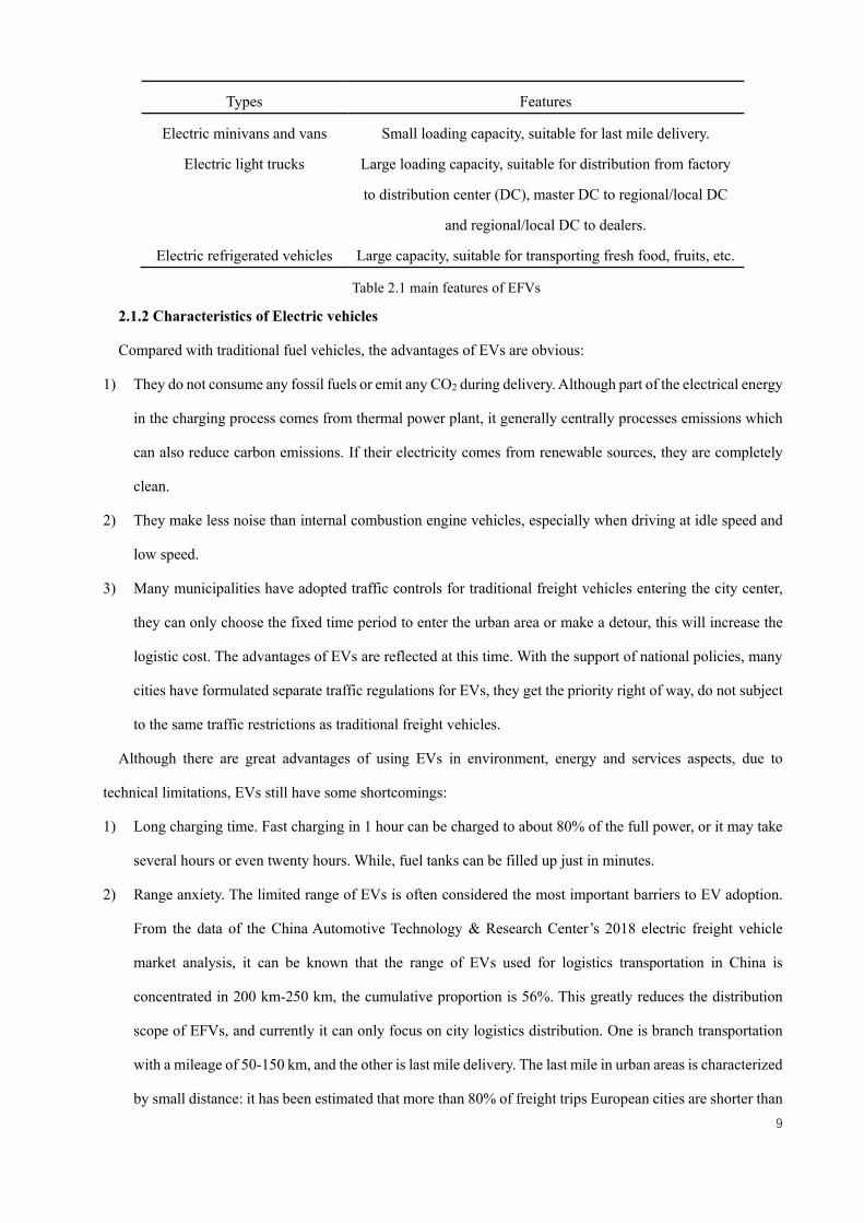
emission brought by the upstream power generation company’s production process. According to statistics
from China National Bureau of Statistics, power generation structure in the past five years as shown in
Figure 1.3.

6
Figure 1.3 annual power generation structure chart
We can see that thermal power generation has always accounted for the largest proportion, but the
percentage has been declining. Thermal power generation accounted for 71% of total power generation in
2018. According to the climate home news, in EU, power generation coming from fossil fuels accounts for
34%. We ignore the carbon emissions caused by water power, wind power and nuclear power, only consider
the carbon emissions caused by thermal power generation. According to the ratio of thermal power to the
entire electricity and the mass balance equation, the expression can be obtained as Eq. (1.2):
𝐸 = 𝛾 ∙ ∑ 𝐹𝑘𝑒 ∙ 𝜆 (1.2)
𝐸 = CO2 emission for a fossil fuel vehicle in a single delivery
𝛾 = the proportion of thermal power in total power generation, here use 71% (2018)
𝐹𝑘𝑒 = electricity consumption per vehicle k, can be obtained by multiplying the unit power consumption
by the distance
λ = carbon emissions per unit of electricity production
When calculating the total logistic cost, the carbon emission cost of vehicles operation is also included in
total cost. We consider the transportation distance, and converts the distance into the carbon emissions of
fossil fuel vehicles and electric vehicles in the distribution process according to fuel consumption and
electricity consumption through their respective conversion factors. Based on the unit carbon emission cost
and the total carbon emission, calculate the carbon emission cost.
0.00% 10.00% 20.00% 30.00% 40.00% 50.00% 60.00% 70.00% 80.00%
thermal power
water power
nuclear power
wind power
solar power
thermal power water power nuclear power wind power solar power2018 71% 17% 4% 5% 3%
2017 71.80% 18.30% 3.80% 4.50% 1.50%
2016 72.20% 19.40% 3.50% 3.90% 1.10%
2015 73.70% 19.40% 2.90% 3.20% 0.70%
2014 75.60% 18.80% 2.30% 2.80% 0.40%
2018
2017
2016
2015
2014

7
1.3 Incentive policies and measures
In the global transportation field, the CO2 emissions caused by road transportation exceed 70% of the total
emissions, of which the emissions from small vehicles (include light van and truck) account for more than 65%,
become the main carbon emission source of the transportation industry, and forecasts project an increasing
number of freight vehicles in city traffic [10]. In order to significantly reduce pollution and emissions from the
transportation sector, some cities have announced that they will restrict internal combustion engine vehicles from
entering the urban areas by delimiting zero-emission zones. Paris, London, Los Angeles, Oslo and Tokyo have
already signed the Fossil Fuel Free Streets Declaration, commit to designate some core urban areas as zero-
emission zones by 2030. Amsterdam announced that the urban central area will be designated as a zero-emission
zone by 2025, allowing only zero-emission vehicles to pass, and plans to expand the zero-emission zone to the
entire city area by 2030. These plans to set the zero-emission zone or the restricted zone for traditional fuel
vehicles send a clear signal to companies and the public, that is, to encourage everyone to buy the electric
vehicles [11].
In 2017, China ministry of transportation issued a road freight industry plan, which clearly pointed out that it
is necessary to strengthen the technical management of urban distribution vehicles and provide convenience for
electric vehicles. In January 2018, the State Council of China issued a document to promote the development of
express logistics, encouraging the express logistics sector to accelerate the use of new energy vehicles or higher
emission standard fuel vehicles, and gradually increase the proportion of new energy vehicles [12].

8
2. Electric vehicles applications in city logistics
In the urban last mile process, as the last link before the product reaches the customer, there are many customer
points, complex distribution routes and congested road conditions that make traditional fuel vehicles run under
uneconomical, high fuel consumption, low speed or idle conditions for a long time, namely causes a lot of carbon
emissions, noise and vibration, and also increase the cost of vehicle. In today’s low-carbon and environmental
protection context, EVs have become the most promising alternative to current distribution vehicles with their
zero-carbon emission, zero pollution and low noise characteristics, and are the main way to realize green logistics.
This chapter defines the related concepts of EVs and analyzes the characteristics and application status of EVs
distribution.
2.1 Relevant concepts
2.1.1 Types of electric vehicles
An electric vehicle is an automobile that is propelled by one or more electric motors, using energy stored in
rechargeable batteries [13]. EVs used in logistic sector can also be called—electric freight vehicles (EFVs). At
present, because of their mileage limit, the application range of EFVs is relatively limited to the field of urban
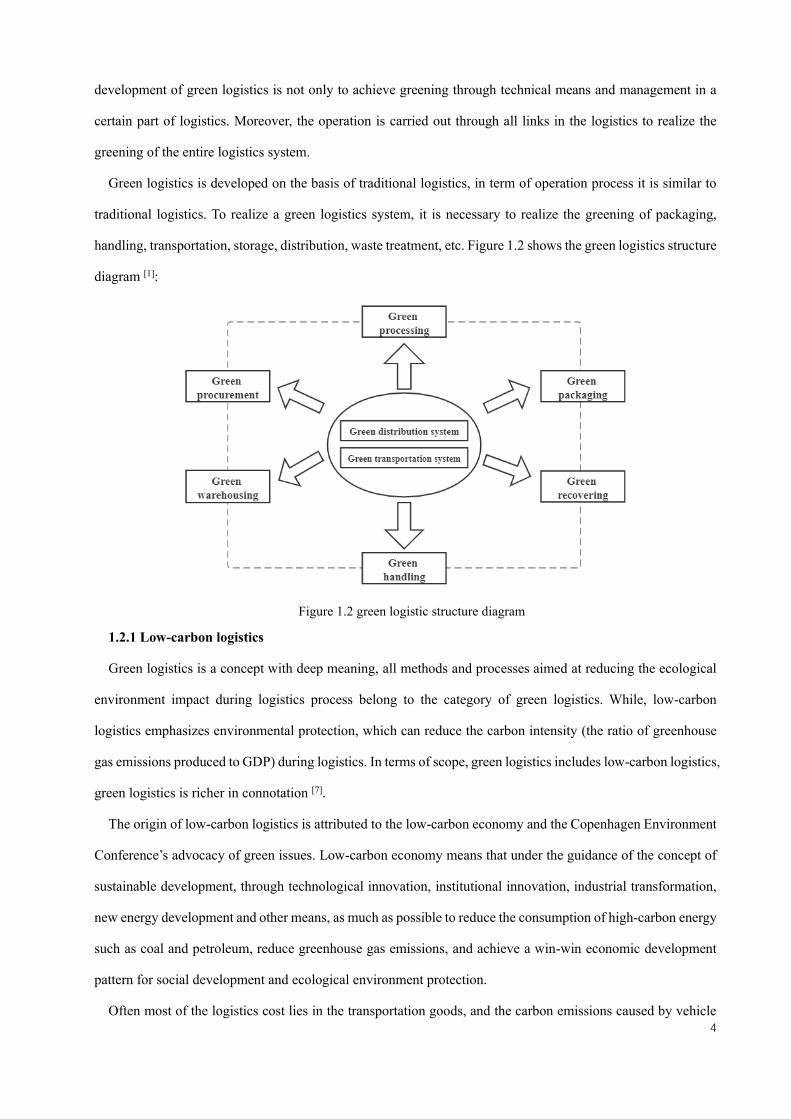
logistics distribution. There are mainly three types: electric minivans and vans, electric light trucks, electric
refrigerated vehicles, shown in figure 2.1. Table 2.1 lists the using features of these three types [14].
Electric Minivans Electric Vans
Electric Light Truck Electric Refrigerated Vehicles
Figure 2.1 main types of EFVs
9
Types Features
Electric minivans and vans Small loading capacity, suitable for last mile delivery.
Electric light trucks Large loading capacity, suitable for distribution from factory
to distribution center (DC), master DC to regional/local DC
and regional/local DC to dealers.
Electric refrigerated vehicles Large capacity, suitable for transporting fresh food, fruits, etc.
Table 2.1 main features of EFVs
2.1.2 Characteristics of Electric vehicles
Compared with traditional fuel vehicles, the advantages of EVs are obvious:
1) They do not consume any fossil fuels or emit any CO2 during delivery. Although part of the electrical energy
in the charging process comes from thermal power plant, it generally centrally processes emissions which
can also reduce carbon emissions. If their electricity comes from renewable sources, they are completely
clean.
2) They make less noise than internal combustion engine vehicles, especially when driving at idle speed and
low speed.
3) Many municipalities have adopted traffic controls for traditional freight vehicles entering the city center,
they can only choose the fixed time period to enter the urban area or make a detour, this will increase the
logistic cost. The advantages of EVs are reflected at this time. With the support of national policies, many
cities have formulated separate traffic regulations for EVs, they get the priority right of way, do not subject
to the same traffic restrictions as traditional freight vehicles.
Although there are great advantages of using EVs in environment, energy and services aspects, due to
technical limitations, EVs still have some shortcomings:
1) Long charging time. Fast charging in 1 hour can be charged to about 80% of the full power, or it may take
several hours or even twenty hours. While, fuel tanks can be filled up just in minutes.
2) Range anxiety. The limited range of EVs is often considered the most important barriers to EV adoption.
From the data of the China Automotive Technology & Research Center’s 2018 electric freight vehicle
market analysis, it can be known that the range of EVs used for logistics transportation in China is
concentrated in 200 km-250 km, the cumulative proportion is 56%. This greatly reduces the distribution
scope of EFVs, and currently it can only focus on city logistics distribution. One is branch transportation
with a mileage of 50-150 km, and the other is last mile delivery. The last mile in urban areas is characterized
by small distance: it has been estimated that more than 80% of freight trips European cities are shorter than

10
80 km, which is compatible with the limited range of EFVs.
3) Backward planning of charging facilities. At present, EFVs have not been widely popularized, and they are
still in the promotion period. The construction of supporting charging facilities means that a large amount
of capital investment is required, but these investments cannot be profitable in the short term. From the
government and enterprise level, there is a lack of motivation for the construction and improvement of
charging facilities, resulting in an unreasonable ratio between the number of EFVs and charging station,
and the problem of difficulty in charging.
2.1.3 Charging modes and charging infrastructures
EVs charging modes can be divided into on-board charging, ground charging, battery swapping and wireless
charging modes. Each charging method has its own characteristics. Here we consider the public charging method
[15]:
1) Fast charging (ground charging)
The direct current (DC) charging station charges the battery directly over a short period of time with a large
current. It has high charging power (60 kw, 120 kw, 200 kw or higher). Charging time is short, usually takes
20mins to 2 hours, charging current is 150-400 A. Fast charging mode work and installation costs are higher
than conventional charging mode. Due to the high current and large impact on the battery, easily heat the battery
and may reduce the battery service life.
2) Normal charging
The alternating current (AC) charging pile delivers alternating current to charger, which converts its stored AC
to DC to charge the battery. Because it is a two-stage power supply process, the charging speed is slow and
usually takes 5 to 8 hours, some even reach 10-20 hours, charging current around 15 A. It is more suitable for
charging in a fixed place or work place at idle time.
3) Wireless charging
The battery can be fast charged without the use of a cable to connect the power supply system. The technology
is based on the electromagnetic induction principle, convert electrical energy into electromagnetic signals, the
vehicle receives the signals and converts into electrical energy. This technology is not yet mature at present.
4) Battery swapping
Battery swapping means the electric vehicles supplement energy by replacing battery packs, eliminating the
delay involved in waiting for charging battery. There are many restrictions of this mode. First, need a large-scale
battery module to ensure the standardization and matching of battery replacement. Secondly, to achieve rapid

11
and convenient battery replacement, require professional staffs and corresponding swapping stations, and the
locations of stations must fully consider the mileage limit of electric vehicles. The battery swapping stations also
require professional technical personnel or mechanical equipment to complete the battery replacement, charging
and maintenance. Due to high investment costs, high technical requirements and lack of professionals, at present,
this mode only used in a few special fields and is not feasible in public.
Battery charging stations are important infrastructures for cities in the future. At present, there are mainly two
types:
1) Centralized charging stations
Provide electric energy supplement for EVs by establishing large-scale centralized professional charging
facilities, similar to the current filling stations.
2) Distributed charging stations
Charing piles are installed in public places (public parking place, shopping mall, highway service area, etc.) and
parking spaces of individual to achieve fast and convenient charging of EVs.
Besides, during the battery charging process, electric energy is converted into chemical energy and stored in
battery. Due to the external environment affects and the chemical nature of the active materials inside battery,
electrical energy cannot be converted into 100% of chemical energy, part of its consumed in other side reactions,
so we need to consider the concept of charging efficiency.
The ratio of the discharged capacity to the input battery capacity when the battery is discharged to a certain
cut-off voltage under certain conditions, this ratio is charging efficiency. Refer to the Electric vehicle charging
technical specifications implemented in Shenzhen in 2011, as shown in Table 2.2.
Charger type Charging efficiency
Off-board charger ≥ 90%
On-board charger 50%~100%
Table 2.2 charging efficiency standard
We mainly consider to use off-board chargers (fixedly installed on the ground, convert AC power from
electricity gird to DC power) to charging battery, from the current mainstream charging equipment, the DC
charging efficiency (fast charging) can reach 95%.
2.2 Application status
Many countries have begun to try and promote the use of EFVs in urban area. Next, we will introduce some
applications in detail.

12
1) In Europe
FREVUE (Freight Electric Vehicles in Urban Europe), the European FP7 project, it is co-funded by the
European Commission under the Seventh Framework Program. It demonstrates the use of EFVs in city logistics
operation in eight European cities [16].
In Milan’s project activity is to improve the urban distribution of goods within the pharmaceutical chain by
implementing a logistics system which will coordinate supply and utilize EVs (e-NV200 Nissan) for delivery.
The system is dedicated to the distribution of medicines to pharmacies located within the Area C (city center).
In order to achieve this goal, Milan established a consolidation center on the outskirts of the city and procured a
(refrigerated) electric freight vehicle for operation. In cooperation with the local freight operator which serve the
59 pharmacies located within Area C, the municipality of Milan estimates that their electric vehicle has the
potential fulfil 20% of the pharmaceutical logistical needs. Through the use of an electric van for pharmaceutical
deliveries, Milan intends to promote this model towards other Italian and European cities.
In Lisbon demonstration project, the Portuguese postal company CTT uses 10 small electric vans (Renault
Kangoo ZOE) for post and parcel operations. EMEL (Lisbon's mobility and parking company) uses 5 small
electric vans for maintenance of the on-street parking and charging facilities.
2) In China
In recent years, the annual growth rate of China's express delivery business has been maintained at around
50%. At present, the entire logistics industry has more than 20 million fuel freight vehicles in stock, the current
market share of electric freight vehicles is only 2%, while the demand for short-distance delivery capacity in
cities has continued to increase, which has created a huge market demand for electric commercial vehicles with
zero emissions and suitable for short-distance distribution.
In November 2017, JD (one of the two massive B2C online retailers in China) logistics announced a joint test
with a number of electric vehicle manufacturers across the country to jointly promote, develop, and introduce
thousands of EVs, and put them into use in 16 large and medium-sized cities. In the next five years, JD logistics
plans to replace all vehicles in the system with EFVs [17].
3) In USA
In September 2019, Amazon placed an order for 100,000 electric delivery vans from EV startup Rivian. The
vans are expected to be on public roads by 2024, with the first coming as soon as 2021, prototypes possibly
arriving as soon as 2020. This order came after Amazon led a 700-million-dollar investment round for Rivian,
which could point to the two companies having a broader relationship as the e-commerce giant builds up a large

13
electric fleet, this is the Amazon’s sweeping plan to tackle climate change.
In January 2020, UPS (American multinational package delivery and supply chain management company)
said its venture capital arm, UPS Ventures, has completed a minority investment in Arrival, along with the
investment in Arrival, UPS also announced a commitment to purchase 10,000 electric vehicles to be built for
UPS with priority access to purchase additional electric vehicles. Arrival is the first commercial vehicle
manufacturer to provide purpose-built electric delivery vehicles to UPS’s specifications and with a production
strategy for global scale. Since 2016, UPS and Arrival have collaborated to develop concepts of different vehicles
sizes. The company previously announced they would develop a state-of-the-art pilot fleet of 35 electric delivery
vehicles to be trialed in London and Paris.
14
3. Vehicle distribution system relevant concepts
The research on EFVs is a new topic in recent years. The current research on electric vehicle distribution
systems mainly focuses on the following three aspects: charging station location allocation problem (CS-LAP),
electric vehicle routing problem (E-VRP) and electric vehicle location-routing problem (E-LRP). Therefore, this
chapter will introduce the basic theory and model of the LAP, the VRP and the LRP respectively.
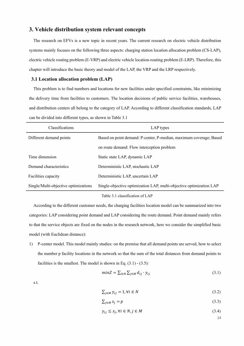
3.1 Location allocation problem (LAP)
This problem is to find numbers and locations for new facilities under specified constraints, like minimizing
the delivery time from facilities to customers. The location decisions of public service facilities, warehouses,
and distribution centers all belong to the category of LAP. According to different classification standards, LAP
can be divided into different types, as shown in Table 3.1
Classifications LAP types
Different demand points Based on point demand: P-center, P-median, maximum coverage; Based
on route demand: Flow interception problem
Time dimension Static state LAP, dynamic LAP
Demand characteristics Deterministic LAP, stochastic LAP
Facilities capacity Deterministic LAP, uncertain LAP
Single/Multi-objective optimizations Single-objective optimization LAP, multi-objective optimization LAP
Table 3.1 classification of LAP
According to the different customer needs, the charging facilities location model can be summarized into two
categories: LAP considering point demand and LAP considering the route demand. Point demand mainly refers
to that the service objects are fixed on the nodes in the research network, here we consider the simplified basic
model (with Euclidean distance):
1) P-center model. This model mainly studies: on the premise that all demand points are served, how to select
the number p facility locations in the network so that the sum of the total distances from demand points to
facilities is the smallest. The model is shown in Eq. (3.1) - (3.5):
𝑚𝑖𝑛𝑍 = ∑ ∑ 𝑑𝑖𝑗 ∙ 𝑦𝑖𝑗𝑗∈𝑀𝑖∈𝑁 (3.1)
s.t.
∑ 𝑦𝑖𝑗 =𝑗∈𝑀 1, ∀𝑖 ∈ 𝑁 (3.2)
∑ 𝑥𝑗 =𝑗∈𝑀 𝑝 (3.3)
𝑦𝑖𝑗 ≤ 𝑥𝑗 , ∀𝑖 ∈ 𝑁, 𝑗 ∈ 𝑀 (3.4)

15
𝑥𝑗 , 𝑦𝑖𝑗 ∈ {0,1}, ∀𝑖 ∈ 𝑁, 𝑗 ∈ 𝑀 (3.5)
𝑀 = candidate facilities locations;
𝑁 = customer points set;
𝑑𝑖𝑗 = distance from point 𝑖 to 𝑗;
𝑝 = numbers of facilities to be constructed;
𝑥𝑗 = {1 0
=1 build facility at point 𝑗;
𝑦𝑖𝑗 = {1 0
=1 customer point 𝑖 is covered by facility 𝑗;
Eq. (3.1) is the objective function of the facilities, which is to minimize the distance. Constraint (3.2)
indicates all the customer points are assigned to a facility; Constraint (3.3) express the number of facilities to be
built; Constraint (3.4) indicates that only open facility can provide services; Constraint (3.5) indicate the 𝑥𝑗,
𝑦𝑖𝑗 are 0-1 variables.
2) Maximum coverage location model. The goal of this model is to select a reasonable location of service
facility to satisfy the largest demand, under the condition that the quantity and service radius of facilities
are known. The model is shown in Eq. (3.6) - (3.10):
𝑚𝑎𝑥𝑍 = ∑ ∑ 𝑑𝑖 ∙ 𝑦𝑖𝑗𝑗∈𝑀𝑖∈𝑁 (3.6)
s.t.
∑ 𝑥𝑗 ≥ 𝑦𝑖𝑗𝑗∈𝑀 , ∀𝑖 ∈ 𝑁 (3.7)
∑ 𝑥𝑗 ≤ 𝑚𝑗∈𝑀 , ∀𝑖 ∈ 𝑁 (3.8)
𝑦𝑖𝑗 ≤ 𝑥𝑗 , ∀𝑖 ∈ 𝑁, 𝑗 ∈ 𝑀 (3.9)
𝑥𝑗 , 𝑦𝑖𝑗 ∈ {0,1}, ∀𝑖 ∈ 𝑁, 𝑗 ∈ 𝑀 (3.10)
𝑀 = candidate facilities locations;
𝑁 = customer points set;
𝑑𝑖𝑗 = demand of point 𝑖;
𝑚 = numbers of facilities to be constructed;
𝑥𝑗 = {1 0
=1 build facility at point 𝑗;
𝑦𝑖𝑗 = {1 0
=1 customer point 𝑖 is covered by facility 𝑗;
Eq. (3.6) is the objective function of the facilities, which is to maximize the demand points covered by
facilities to be built. Constraint (3.7) indicates satisfy the customer point 𝑖 just when facility build at point 𝑗;

16
Constraint (3.8) express the number of facilities to be built; Constraint (3.9) indicates that only open facility can
provide services; Constraint (3.10) indicate the 𝑥𝑗, 𝑦𝑖𝑗 are 0-1 variables.
3) Flow interception location model. If customer demand is distributed on the traffic route in the network, this
is a location model based on route demand. This model refers to how to select the service facilities location
under the premise that the routes, the number of service facilities and the demand are known, so that the
service facilities can intercept the maximum total demand. The model is shown in Eq (3.11) - (3.14):
𝑚𝑎𝑥𝑍 = ∑ 𝑓𝑞𝑞∈𝑄 ∙ 𝑦𝑞 (3.11)
s.t.
∑ 𝑥𝑗 = 𝑚𝑗∈𝑉 (3.12)
∑ 𝑥𝑗 ≥ 𝑦𝑞𝑉𝑞∈𝐴 , ∀𝑞 ∈ 𝑄 (3.13)
𝑥𝑗 , 𝑦𝑞 ∈ {0,1}, ∀𝑗 ∈ 𝑉, 𝑞 ∈ 𝑄 (3.14)
𝑉 = set of all nodes in the network;
𝐴 = set of all arcs in the network;
𝑄 = set of all routes whose traffic flows are not 0;
𝑓𝑞 = the traffic flow at 𝑞 route;
𝑉𝑞 = set of nodes at 𝑞 route;
𝑚 = numbers of facilities to be constructed;
𝑥𝑗 = {1 0
=1 build facility at node 𝑗;
𝑦𝑞 = {1 0
=1 at least build one facility on the route 𝑞;
Eq. (3.11) is the objective function, indicates that service facilities to be built can meet the largest demand in
the routes. Constraint (3.12) express the number of facilities to be built; Constraint (3.13) indicates that only
open facility can provide services; Constraint (3.10) indicate the 𝑥𝑗, 𝑦𝑞 are 0-1 variables.
17
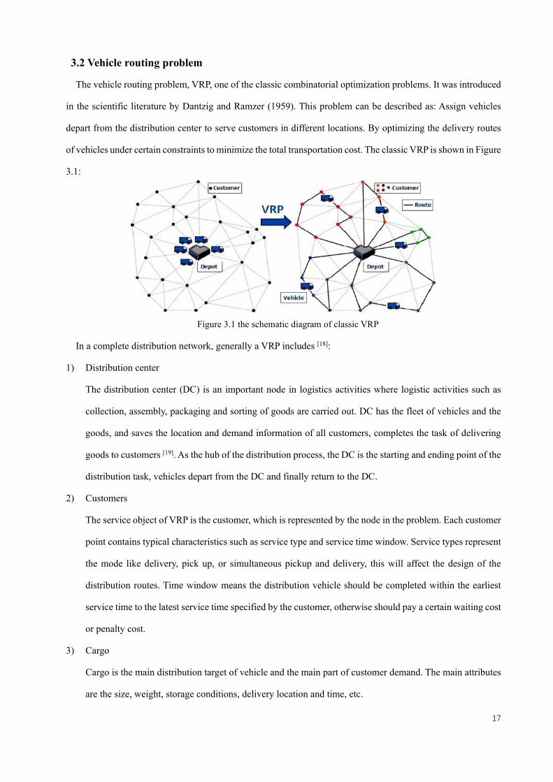
3.2 Vehicle routing problem
The vehicle routing problem, VRP, one of the classic combinatorial optimization problems. It was introduced
in the scientific literature by Dantzig and Ramzer (1959). This problem can be described as: Assign vehicles
depart from the distribution center to serve customers in different locations. By optimizing the delivery routes
of vehicles under certain constraints to minimize the total transportation cost. The classic VRP is shown in Figure
3.1:
Figure 3.1 the schematic diagram of classic VRP
In a complete distribution network, generally a VRP includes [18]:
1) Distribution center
The distribution center (DC) is an important node in logistics activities where logistic activities such as
collection, assembly, packaging and sorting of goods are carried out. DC has the fleet of vehicles and the
goods, and saves the location and demand information of all customers, completes the task of delivering
goods to customers [19]. As the hub of the distribution process, the DC is the starting and ending point of the
distribution task, vehicles depart from the DC and finally return to the DC.
2) Customers
The service object of VRP is the customer, which is represented by the node in the problem. Each customer
point contains typical characteristics such as service type and service time window. Service types represent
the mode like delivery, pick up, or simultaneous pickup and delivery, this will affect the design of the
distribution routes. Time window means the distribution vehicle should be completed within the earliest
service time to the latest service time specified by the customer, otherwise should pay a certain waiting cost
or penalty cost.
3) Cargo
Cargo is the main distribution target of vehicle and the main part of customer demand. The main attributes
are the size, weight, storage conditions, delivery location and time, etc.

18
4) Vehicles
In the VRP, the vehicles complete the task of goods distribution or collection service between the DC and
customer points. VRP need to consider the attributes of vehicles and goods, and accurately arrange suitable
vehicles, which can improve resource utilization and reduce distribution costs.
5) Constraints
Constraints refer to the conditions that must be satisfied during the vehicle delivery process. Basic
constraints generally include loading capacity constraints, travel distance constraints, time window
constraints, etc.
6) Objective functions.
The objective function is the purpose of the model, which can be divided into single-objective optimization
and multi-objective optimization. In actual VRP, they are all multi-objective optimization problems. The
optimization goals generally include: the shortest driving distance, the least cost, the least number of
vehicles, etc.
On the basic of classic VRP, it can be complicated by adding different constraints or other restrictive elements,
the main classifications are shown in the table 3.2
Analysis elements VRP types
Loading capacity Capacitated VRP, VRP without restriction of loading capacity
Distribution center number VRP with single DC, VRP with multiple DCs
Vehicles types VRP with single vehicle type, VRP with multiple vehicle types
Customer time demand VRP without time window, VRP with time window (soft/hard time window)
Distribution method Delivery type, simultaneous delivery and pick up
Distribution information Static VRP, dynamic VRP
Number of objective functions Single-objective optimization, multi-objective optimization
Table 3.2 different classifications of VRP
The classic VRP model is shown in Eq. (3.6) - (3.12):
𝑚𝑖𝑛𝑍 = ∑ ∑ 𝑐𝑖𝑗 ∙ 𝑥𝑖𝑗𝑗∈𝑉𝑖∈𝑉 (3.6)
s.t. ∑ 𝑥𝑖𝑗 = 1, ∀𝑗 ∈ 𝑁 ∪ {0} 𝑖∈𝑉 (3.7)
∑ 𝑥𝑖𝑗 = 1, ∀𝑖 ∈ 𝑁 ∪ {0} 𝑗∈𝑉 (3.8)
∑ 𝑥𝑖0 = 𝐾𝑖∈𝑉 (3.9)
∑ 𝑥0𝑗 = 𝐾𝑗∈𝑉 (3.10)

19
∑ ∑ 𝑥𝑖𝑗 ≥ 𝑟(𝑆), ∀𝑆 ⊆ 𝑉\{0}, 𝑆 ≠ ∅𝑗∈𝑆𝑖∉𝑆 (3.11)
𝑥𝑖𝑗 ∈ {0,1}, ∀𝑖, 𝑗 ∈ 𝑉 (3.12)
{0} = distribution center node;
𝑐𝑖𝑗 = cost of going from node 𝑖 to 𝑗;
𝐾 = numbers of available vehicles;
𝑥𝑖𝑗 = {1
0 =1 arc is going from node 𝑖 to 𝑗;
𝑟(𝑆) = the minimum number of vehicles needed to serve set 𝑆;
Eq. (3.6) is the objective function, indicates the minimum delivery cost; constraints (3.7), (3.8) state that
exactly one arc enters and exactly one leaves each customer point, respectively; constraints (3.9), (3.10) indicate
the number of vehicles leaving the depot is the same as the number entering; constraint (3.11) is the capacity cut
constraints, which impose that the routes must be connected and that the demand on each route must not exceed
the vehicle capacity; constraints (3.12) indicates 𝑥𝑖𝑗 is 0-1 variables.
3.3 Location-Routing problem
Location-routing problem (LRP) can be described as: given a series of customer points and several potential
facilities locations, by comprehensively consider the LAP of the facilities and the VRP in the same problem, the
goal is to obtain the facilities locations and vehicle routes with minimum cost or distance under the certain
constraints. Classic LRP diagram is shown in Figure 3.2, Table 3.3 shows the classifications of LRP:
Figure 3.2 the schematic diagram of classic LRP
Analysis elements LRP types
Facilities number LRP with single facility, LRP with multiple facilities
Vehicles types LRP with single vehicle type, LRP with multiple vehicles types
Time window LRP without time window, LRP with time window (soft/hard time window)
20
Supply/demand characteristics Static LRP, dynamic LRP
Number of objective functions Single-objective optimization, multi-objective optimization
Table 3.3 classifications of LRP
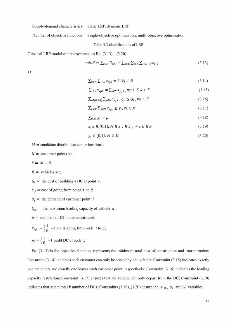
Classical LRP model can be expressed as Eq. (3.13) – (3.20):
𝑚𝑖𝑛𝑍 = ∑ 𝐺𝑖𝑦𝑖𝑖∈𝑀 + ∑ ∑ ∑ 𝑐𝑖𝑗𝑥𝑖𝑗𝑘𝑗∈𝑆𝑖∈𝑆𝑘∈𝐾 (3.13)
s.t.
∑ ∑ 𝑥𝑖𝑗𝑘𝑖∈𝑆𝑘∈𝐾 = 1, ∀𝑗 ∈ 𝑁 (3.14)
∑ 𝑥𝑖𝑝𝑘 =𝑖∈𝑆 ∑ 𝑥𝑝𝑗𝑘𝑗∈𝑆 , ∀𝑝 ∈ 𝑆, 𝑘 ∈ 𝐾 (3.15)
∑ ∑ 𝑥𝑖𝑗𝑘𝑗∈𝑁𝑖∈𝑁∪{0} ∙ 𝑞𝑗 ≤ 𝑄𝑘 , ∀𝑘 ∈ 𝐾 (3.16)
∑ ∑ 𝑥𝑖𝑗𝑘𝑗∈𝑁𝑘∈𝐾 ≥ 𝑦𝑖 , ∀𝑖 ∈ 𝑀 (3.17)
∑ 𝑦𝑖𝑖∈𝑀 = 𝑝 (3.18)
𝑥𝑖𝑗𝑘 ∈ {0,1}, ∀𝑖 ∈ 𝑆, 𝑗 ∈ 𝑆, 𝑗 ≠ 𝑖, 𝑘 ∈ 𝐾 (3.19)
𝑦𝑖 ∈ {0,1}, ∀𝑖 ∈ 𝑀 (3.20)
𝑀 = candidate distribution center locations;
𝑁 = customer points set;
𝑆 = 𝑀 ∪ 𝑁;
𝐾 = vehicles set;
𝐺𝑖 = the cost of building a DC at point 𝑖;
𝑐𝑖𝑗 = cost of going from point 𝑖 to 𝑗;
𝑞𝑗 = the demand of customer point 𝑗
𝑄𝑘 = the maximum loading capacity of vehicle 𝑘;
𝑝 = numbers of DC to be constructed;
𝑥𝑖𝑗𝑘 = {1 0
=1 arc is going from node 𝑖 to 𝑗;
𝑦𝑖 = {1 0
=1 build DC at node 𝑖;
Eq. (3.13) is the objective function, represents the minimum total cost of construction and transportation;
Constraint (3.14) indicates each customer can only be served by one vehicle; Constraint (3.15) indicates exactly
one arc enters and exactly one leaves each customer point, respectively; Constraint (3.16) indicates the loading
capacity restriction; Constraint (3.17) ensures that the vehicle can only depart from the DC; Constraint (3.18)
indicates that select total P number of DCs; Constraints (3.19), (3.20) ensure the 𝑥𝑖𝑗𝑘, 𝑦𝑖 are 0-1 variables.

21
4. Location-routing problem of electric vehicles model formulation
4.1 Model description
With the improvement of people’s awareness of environmental protection and the countries’ promotion of new
energy vehicles, EVs are expected to gradually replace traditional fuel vehicles and change the current status of
cargo transportation. Therefore, for logistics companies, the problem is how to upgrade their transport vehicles
with minimal cost. Meanwhile, because EFVs have not yet widely used, and the construction of charging stations
is not complete, logistics companies need to consider where to charge when using EFVs for distribution.
Compared with traditional LRP, we consider the following elements in this model:
1) Distribution center.
The distribution center is a distribution facility where goods are equipped according to customer
requirements and delivered to users. In this model, we have one distribution center, as the starting point of
transportations, equipped with a certain number of EFVs, they return to the distribution center after
completing the delivery task. Different from traditional distribution centers, in this study have slow charging
facilities in order to charging EFVs at night to save charging costs.
2) Electric freight vehicles.
According to types of vehicles, LRP can be divided into single vehicle type and multiple vehicles types.
Considering that there are not so many types of EFVs on the market at present, meanwhile, logistics
companies are in the status quo of partial conversion of delivery vehicles from traditional fuel vehicles to
EFVs, so companies generally choose one type of vehicle when purchasing EFVs. Therefore, we will
consider only one type of vehicle in our model. EFVs distribution not only needs to consider the maximum
load and maximum mileage, but also consider whether and where they need to be charged during delivery
process. These also make the LRP of EFVs more complicated than traditional fuel vehicles.
3) Charging stations
Unlike general LRP, the location problem of EVs is charging stations. Companies need to select suitable
locations from several alternative locations where charging stations can be built. The EFVs can arrive at
the charging station for power replenishment during delivery, while minimizing the total cost of location
selection and transportation.
4) Customers
In this model, the customer mainly including retail stores, supermarkets, etc. The positions of customers in
the transportation network are important. The entire transportation network routes will change with the

22
demand or time window of the customer points request.
Through the model introduction in section 4.1, we can know our LRP model is a special case of the traditional
LRP model. The same point is both contain the location selection and routing arrangement, the difference is: in
the traditional LRP model the location selection is distribution center, while the object of the electric vehicle
LRP location selection is the charging station. Figure 4.1 (1), (2) part represents the classic LRP model and
electric vehicle LRP model [20].
Figure 4.1 typical routes of traditional LRP and electric vehicle LRP
The mathematical model of the electric vehicle LRP with time windows is described as:
𝐺 = {𝑉, 𝐸} is a distribution network composed of point sets and arc sets, set 𝑉 = 𝑁 ∪ 𝐵 ∪ 𝑂 includes all
the nodes in the network. 𝑁 is the set of customer nodes, 𝐵 is the set of charging stations nodes, 𝑂 is
distribution center.
Since the current charging facilities are not yet complete, in the initial stage, company can also consider the
location problem and choose the location and number of charging stations with lowest total cost from the
alternative charging stations. The confirmed information of customer points including the locations, demand
amounts and time windows. The setting value of objective function is the minimum total cost. Company arrange
the EFVs depart from distribution center, to serve the customer points under the constraint of maximum load
capacity; Meanwhile, EFVs need to visit all customer points within the specified time window, otherwise they
should pay the waiting cost or penalty cost. In addition, due to the short mileage of EFVs, they perhaps need to
visit charging stations for power replenishment, so that there is sufficient power to continue to deliver the next
customer. Until all customer points have been visited, they will go back to the distribution center.
4.2 Assumptions and notations of model
Since the electric vehicles LRP model for urban freight distribution is derived from the traditional LRP model

23
of traditional fuel vehicles, and considering the complexity of transforming actual problems into mathematical
models, we make the following assumptions to reduce the complexity of calculations:
1) A single distribution center, multiple demand (customer) points.
2) All the customer points’ locations, demand amounts and time windows are known quantitative data, and
will not change dynamically.
3) A customer point can be served only once.
4) The demand amount of goods at customer points should not exceed the vehicle’s capacity.
5) Vehicles depart from the distribution center, return to it after completing the distribution tasks.
6) All vehicles run at a constant speed, regardless of traffic conditions.
7) All vehicles are the same type, with the same capacity limitation, battery capacity and maximum mileage.
8) Vehicles is fully charged after leaving the distribution center or visiting the charging stations.
9) Vehicles have a fixed power consumption coefficient, and the power consumption is proportional to the
driving distance.
10) The charging efficiency of vehicles at the charging station is fixed, the charging time is proportional to the
required charging capacity.
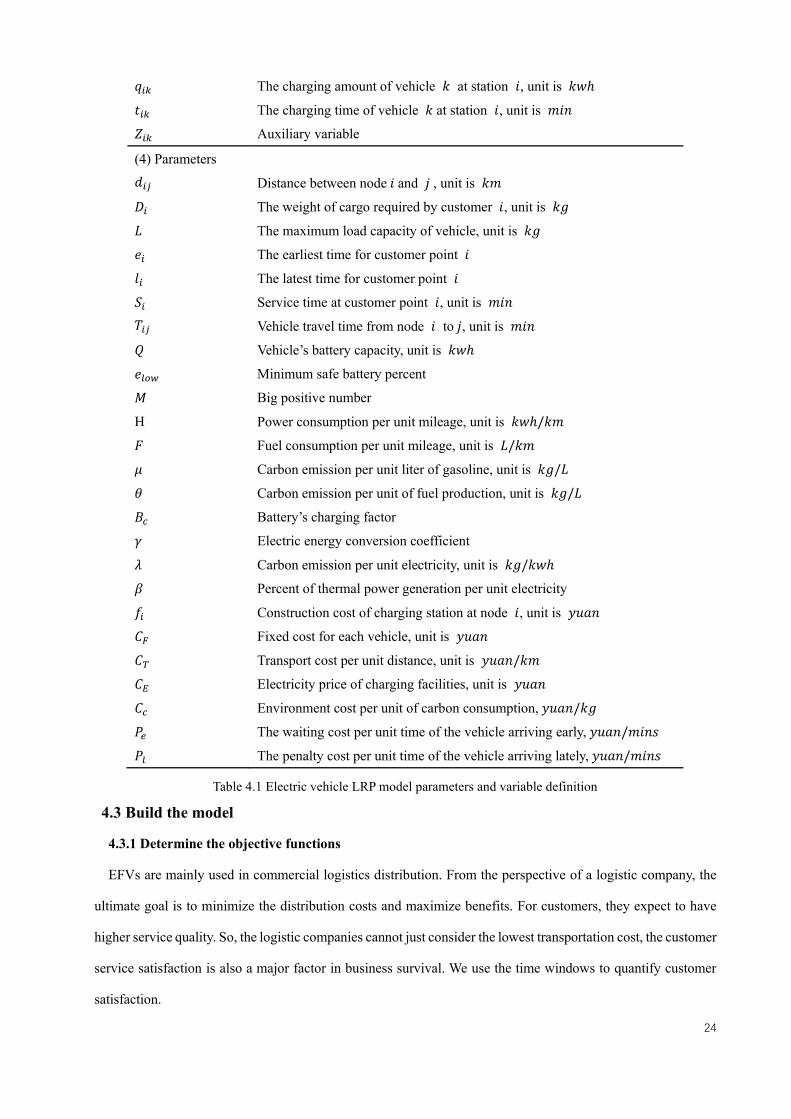
In order to facilitate the accurate description of the model, the parameters and variables involved in model are
defined in Table 4.1.
Symbols Meanings
(1) Sets
𝑂 A single distribution center, {0}
𝑁 Set of customers point (nodes), 𝑁 = {1,2 … 𝑛}
𝐵 Set of battery charging stations, 𝐵 = {1,2. . . 𝑏}
𝑉 Set of nodes, 𝑉 = 𝑁 ∪ 𝐵 ∪ 𝑂
𝐾 Set of vehicles, 𝐾 = {1,2. . . 𝑘}
(2) Decision variables 𝑥𝑖𝑗𝑘 When vehicle 𝑘 finish task from point 𝑖 to 𝑗: = 1
Otherwise = 0
𝑦𝑖 When a charging station is established at node 𝑖 , = 1
Otherwise = 0
(3) Variables
𝑎𝑟𝑟𝑖𝑘 The moment vehicle 𝑘 arrives at node 𝑖
𝑙𝑒𝑣𝑖𝑘 The moment vehicle 𝑘 leaves from node 𝑖
𝑟𝑒1𝑖𝑘 The residual power of vehicle 𝑘 when arrive at node 𝑖, unit is 𝑘𝑤ℎ
𝑟𝑒2𝑖𝑘 The residual power of vehicle 𝑘 when leave from node 𝑖, unit is 𝑘𝑤ℎ
24
𝑞𝑖𝑘 The charging amount of vehicle 𝑘 at station 𝑖, unit is 𝑘𝑤ℎ
𝑡𝑖𝑘 The charging time of vehicle 𝑘 at station 𝑖, unit is 𝑚𝑖𝑛
𝑍𝑖𝑘 Auxiliary variable
(4) Parameters 𝑑𝑖𝑗 Distance between node 𝑖 and 𝑗 , unit is 𝑘𝑚
𝐷𝑖 The weight of cargo required by customer 𝑖, unit is 𝑘𝑔
𝐿 The maximum load capacity of vehicle, unit is 𝑘𝑔
𝑒𝑖 The earliest time for customer point 𝑖
𝑙𝑖 The latest time for customer point 𝑖
𝑆𝑖 Service time at customer point 𝑖, unit is 𝑚𝑖𝑛 𝑇𝑖𝑗 Vehicle travel time from node 𝑖 to 𝑗, unit is 𝑚𝑖𝑛
𝑄 Vehicle’s battery capacity, unit is 𝑘𝑤ℎ
𝑒𝑙𝑜𝑤 Minimum safe battery percent
𝑀 Big positive number
H Power consumption per unit mileage, unit is 𝑘𝑤ℎ/𝑘𝑚
𝐹 Fuel consumption per unit mileage, unit is 𝐿/𝑘𝑚
𝜇 Carbon emission per unit liter of gasoline, unit is 𝑘𝑔/𝐿
𝜃 Carbon emission per unit of fuel production, unit is 𝑘𝑔/𝐿
𝐵𝑐 Battery’s charging factor
𝛾 Electric energy conversion coefficient
𝜆 Carbon emission per unit electricity, unit is 𝑘𝑔/𝑘𝑤ℎ
𝛽 Percent of thermal power generation per unit electricity
𝑓𝑖 Construction cost of charging station at node 𝑖, unit is 𝑦𝑢𝑎𝑛
𝐶𝐹 Fixed cost for each vehicle, unit is 𝑦𝑢𝑎𝑛
𝐶𝑇 Transport cost per unit distance, unit is 𝑦𝑢𝑎𝑛/𝑘𝑚
𝐶𝐸 Electricity price of charging facilities, unit is 𝑦𝑢𝑎𝑛
𝐶𝑐 Environment cost per unit of carbon consumption, 𝑦𝑢𝑎𝑛/𝑘𝑔
𝑃𝑒 The waiting cost per unit time of the vehicle arriving early, 𝑦𝑢𝑎𝑛/𝑚𝑖𝑛𝑠
𝑃𝑙 The penalty cost per unit time of the vehicle arriving lately, 𝑦𝑢𝑎𝑛/𝑚𝑖𝑛𝑠
Table 4.1 Electric vehicle LRP model parameters and variable definition
4.3 Build the model
4.3.1 Determine the objective functions
EFVs are mainly used in commercial logistics distribution. From the perspective of a logistic company, the
ultimate goal is to minimize the distribution costs and maximize benefits. For customers, they expect to have
higher service quality. So, the logistic companies cannot just consider the lowest transportation cost, the customer
service satisfaction is also a major factor in business survival. We use the time windows to quantify customer
satisfaction.

25
With the increasing awareness of environmental protection, the goals pursued by the logistic companies are
constantly updated, considering reducing the exhaust emissions of vehicles during delivery process.
Therefore, our goal is to minimize the total cost, which include the six costs as following:
1) The construction cost of charging station.
In the research phase of location selection for EFVs charging stations, the construction cost of charging
station is the most important expenditure. In reality, the construction cost is affected by many factors, such
as the construction area of charging station. Here we consider the total cost of building the charging stations
as shown in Eq. (4.1):
𝑍𝑠𝑡𝑎𝑡𝑖𝑜𝑛 = ∑ 𝑓𝑖 ∙ 𝑦𝑖𝑖𝜖𝐵 (4.1)
2) The fixed cost per each vehicle
𝑍𝑓𝑖𝑥𝑒𝑑 = ∑ 𝐶𝐹 ∙ 𝑘𝑘𝜖𝐾 (4.2)
3) The transport cost of vehicle
The most common objective function in the VRP is the shortest distance or the lowest cost. Generally
speaking, the transport cost will increase proportionally as the distance increases. The transport cost as Eq.
(4.3):
𝑍𝑡𝑟𝑎𝑛𝑠𝑝𝑜𝑟𝑡 = ∑ ∑ ∑ 𝐶𝑇 ∙ 𝑑𝑖𝑗 ∙ 𝑥𝑖𝑗𝑘𝑘∈𝐾𝑗∈𝑉𝑖≠𝑗
𝑖∈𝑉 (4.3)
4) The charging cost of vehicles
If need battery charging during distribution process of using EFVs, we should consider the charging cost.
Generally, the charging cost is related to the amount of charging required for EFVs. The charging cost
represents as Eq. (4.4)
𝑍𝑐ℎ𝑎𝑟𝑔𝑖𝑛𝑔 = ∑ ∑ 𝐶𝐸 ∙ 𝑞𝑖𝑘 ∙ 𝑦𝑖𝑘∈𝐾𝑖∈𝑉 (4.4)
5) The environmental cost
The environmental costs are mainly reflected in carbon emissions, in section 1.2.2, we introduced in detail
the calculation standards of carbon emissions for traditional fuel vehicles and EVs. The environment cost
of fossil fuel vehicle and EVs are expressed as Eq. (4.5), (4.6):
𝑍𝑐𝑎𝑟𝑏𝑜𝑛 = 𝐶𝑐 ∙ (𝜇 + 𝜃) ∑ ∑ ∑ 𝑥𝑖𝑗𝑘 ∙ 𝑑𝑖𝑗 ∙ 𝐹𝑗∈𝑉𝑗≠𝑖
𝑖∈𝑉𝑘∈𝐾 (4.5)
𝑍𝑐𝑎𝑟𝑏𝑜𝑛 = 𝛽 ∙ 𝐶𝑐 ∙ 𝛾 ∑ ∑ ∑ 𝑥𝑖𝑗𝑘 ∙ 𝑑𝑖𝑗 ∙ 𝐻𝑗∈𝑉𝑗≠𝑖
𝑖∈𝑉𝑘∈𝐾 (4.6)
6) The penalty cost of violating the time windows

26
Taking into account the timeliness requirements of customers for delivery services, we take the time effect
cost that is caused by the violation of the customer’s time window constraint, the penalty cost, into the total
logistic cost. Time window restrictions can be divided into hard time windows and soft time windows.
Considering the complexity of the actual delivery process, here we use the soft time window limit, [𝑒𝑖 , 𝑙𝑖]
represents the soft time window of customer 𝑖. 𝑃𝑒 is the penalty cost per unit time for the early arrival of
vehicle, 𝑃𝑙 is the penalty cost per unit time for vehicle late arrival.
The penalty cost function is Eq. (4.7), (4.8):
𝑃(𝑎𝑟𝑟𝑖𝑘) = {
𝑃𝑒(𝑒𝑖 − 𝑎𝑟𝑟𝑖𝑘), 𝑎𝑟𝑟𝑖𝑘 ≤ 𝑒𝑖
0, 𝑒𝑖 ≤ 𝑎𝑟𝑟𝑖𝑘 ≤ 𝑙𝑖
𝑃𝑙(𝑎𝑟𝑟𝑖𝑘 − 𝑙𝑖), 𝑎𝑟𝑟𝑖𝑘 ≥ 𝑙𝑖
(4.7)
𝑍𝑝𝑒𝑛𝑎𝑙𝑡𝑦 = ∑ ∑ 𝑃(𝑎𝑟𝑟𝑖𝑘)𝑘∈𝐾𝑖∈𝑁 (4.8)
4.3.2 Mathematical model
Based on the above model assumptions and notations, combined with the relevant analysis of the objective
function, the mathematical model can be described as Eq. (4.9)
𝑚𝑖𝑛𝑍 = 𝑍𝑠𝑡𝑎𝑡𝑖𝑜𝑛 + 𝑍𝑓𝑖𝑥𝑒𝑑 + 𝑍𝑡𝑟𝑎𝑛𝑠𝑝𝑜𝑟𝑡 + 𝑍𝑐ℎ𝑎𝑟𝑔𝑖𝑛𝑔 + 𝑍𝑐𝑎𝑟𝑏𝑜𝑛 + 𝑍𝑝𝑒𝑛𝑎𝑙𝑡𝑦 (4.9)
s.t.
∑ ∑ 𝑥𝑖𝑗𝑘 = ∑ ∑ 𝑥𝑗𝑖𝑘 = 1𝑘∈𝐾𝑖∈𝑉𝑖≠𝑗
𝑘∈𝐾𝑖∈𝑉𝑖≠𝑗
(4.10)
∑ 𝑥0𝑗𝑘 = ∑ 𝑥𝑗0𝑘 ≤ 1𝑗∈𝑁∪𝐵𝑗∈𝑁∪𝐵 , ∀𝑘 ∈ 𝐾 (4.11)
∑ ∑ 𝑥𝑖𝑗𝑘 ≤ 𝑦𝑗 ∙ 𝑀𝑘∈𝐾𝑖∈𝑉𝑖≠𝑗
(4.12)
∑ 𝑥𝑖𝑗𝑘 = ∑ 𝑥𝑗𝑖𝑘, ∀𝑗 ∈ 𝑁 ∪ 𝐵, 𝑘 ∈ 𝐾𝑖∈𝑉𝑖≠𝑗
𝑖∈𝑉𝑖≠𝑗
(4.13)
∑ ∑ 𝐷𝑖𝑗∈𝐵𝑖∈𝑉𝑖≠𝑗
∙ 𝑥𝑖𝑗𝑘 ≤ 𝐿, ∀𝑘 ∈ 𝐾 (4.14)
𝑥0𝑗𝑘 = 0, ∀𝑗 ∈ 𝐵, 𝑘 ∈ 𝐾 (4.15)
𝑙𝑒𝑣𝑖𝑘 = 𝑎𝑟𝑟𝑖𝑘 + 𝑆𝑖 , ∀𝑖 ∈ 𝑁, 𝑘 ∈ 𝐾 (4.16)
𝑙𝑒𝑣𝑖𝑘 = 𝑎𝑟𝑟𝑖𝑘 + 𝑡𝑖𝑘, ∀𝑖 ∈ 𝐸, 𝑘 ∈ 𝐾 (4.17)
𝑎𝑟𝑟𝑗𝑘 = ∑ 𝑥𝑖𝑗𝑘 ∙ (𝑙𝑒𝑣𝑖𝑘 + 𝑇𝑖𝑗), ∀𝑗 ∈ 𝑁 ∪ 𝐵, 𝑘 ∈ 𝐾𝑖∈𝑉𝑖≠𝑗
(4.18)
𝑞𝑖𝑘 = 𝑡𝑖𝑘 ∙ 𝐵𝑐 ∙ 𝑦𝑖 , ∀𝑖 ∈ {0} ∪ 𝐵, 𝑘 ∈ 𝐾 (4.19)
𝑟𝑒20𝑘 = 𝑄, ∀𝑘 ∈ 𝐾 (4.20)
𝑟𝑒2𝑖𝑘 = 𝑦𝑖 ∙ 𝑄, ∀𝑖 ∈ 𝐵, ∀𝑘 ∈ 𝐾 (4.21)
𝑟𝑒2𝑖𝑘 = 𝑟𝑒1𝑖𝑘 , ∀𝑖 ∈ 𝑁, 𝑘 ∈ 𝐾 (4.22)
27
𝑟𝑒1𝑖𝑘 ≥ 0, ∀𝑖 ∈ 𝑉, 𝑘 ∈ 𝐾 (4.23)
𝑟𝑒1𝑗𝑘 = ∑ 𝑥𝑖𝑗𝑘 ∙ (𝑟𝑒2𝑖𝑘 − 𝐻 ∙ 𝑑𝑖𝑗)𝑖∈𝑉𝑖≠𝑗
, ∀𝑗 ∈ 𝑉, 𝑘 ∈ 𝐾 (4.24)
𝑟𝑒1𝑗𝑘 ≥ 𝑒𝑙𝑜𝑤 ∙ 𝑄, 𝑗 ∈ 𝑉, 𝑘 ∈ 𝐾 (4.25)
𝑞𝑖𝑘 = (Q − 𝑟𝑒1𝑖𝑘) ∙ 𝑦𝑖 , ∀𝑖 ∈ 𝐵, 𝑘 ∈ 𝐾 (4.26)
𝑞𝑖𝑘 = 0, ∀𝑖 ∈ 𝑁, 𝑘 ∈ 𝐾 (4.27)
e𝑖 ≤ 𝑎𝑟𝑟𝑖𝑘 ≤ 𝑙𝑖 , ∀𝑖 ∈ 𝑁 ∪ 𝐵, 𝑘 ∈ 𝐾 (4.28)
𝑍𝑖𝑘 − 𝑍𝑗𝑘 + 𝑛 ∙ 𝑥𝑖𝑗𝑘 ≤ 𝑛 − 1, ∀𝑖 ∈ 𝑉, 𝑗 ≠ 𝑖, 𝑗 ∈ 𝑁, 𝑘 ∈ 𝐾 (4.29)
𝑍𝑖𝑘 ≥ 0, ∀𝑖 ∈ 𝑉, 𝑘 ∈ 𝐾 (4.30)
𝑥𝑖𝑗𝑘 ∈ {0,1}, ∀𝑖, 𝑗 ∈ 𝑉, 𝑖 ≠ 𝑗, 𝑘 ∈ 𝐾 (4.31)
𝑦𝑖 ∈ {0,1}, ∀𝑖 ∈ 𝐵 (4.32)
Eq. (4.9) is the objective function, indicates the minimum total distribution cost.
Constraint (4.10) states that each customer point can be served only once.
Constraint (4.11) states that each vehicle departs from DC, return to DC after completing the distribution tasks.
Constraint (4.12) indicates EV can only charging battery at the position where a charging station is built.
Constraint (4.13) exactly one arc enters and exactly one leaves each customer point.
Constraint (4.14) states that the demand on each route must not exceed the vehicle capacity.
Constraint (4.15) states that vehicle cannot go to charging station directly after departing from DC.
Constraint (4.16) express the moment of vehicle depart from the customer point 𝑖.
Constraint (4.17) express the moment of vehicle depart from the charging station 𝑖.
Constraint (4.18) is the moment of vehicle arriving customer point 𝑖.
Constraint (4.19) indicates the charging time of EFVs, affected by charging amount and charging efficiency.
Constraint (4.20), (4.21) indicates that vehicle depart from the DC and charging station at the maximum power.
Constraint (4.22) indicates that the electric quantity of vehicle will not change at customer point.
Constraint (4.23) ensures the electric quantity always positive at any nodes.
Constraint (4.24) calculates the remaining battery after vehicle arriving node.
Constraint (4.25) ensures the vehicle remaining power to each node is not less than the minimum safe power.
Constraint (4.26) calculates the electric quantity needed to charge when vehicle visit charging station.
Constraint (4.27) ensure that vehicle cannot be charged at customer point.
Constraint (4.28) is the time window constraint.
Constraint (4.29), (4.30) indicate the sub-loop elimination.

28
Constraint (4.31), (4.32) define the decision variable, 𝑥𝑖𝑗𝑘 , 𝑦𝑖 are both 0-1 variables.
29
5.Algorithm design for electric vehicle location-routing problem
5.1 Algorithm overview
We start from the perspective of using EFVs during distribution, meanwhile, conducts research on charging
station location problem and distribution routes optimization, these problems can be called location-routing
problem (LRP) of electric vehicle, which is derived from traditional LRP research.
Vehicle routing problem (VRP) was first introduced in the scientific literature 61 years ago, during this long
time period, many scholars have studied VRP and its various derivative models and algorithms. It is one of the
classic combinatorial optimization problems, and the NP-hard problem (non-deterministic polynomial-time
hardness) [21]. The LRP of EVs is a combination of VRP and LAP, so LRP is also an NP-hard problem. The
existing algorithms for solving NP-hard problems including two categories: Exact algorithms and heuristic
algorithms. Heuristic algorithms can be divided into classical heuristic algorithms and metaheuristic algorithms.
The exact algorithms are mainly used to solve small-scale problems, as the scale of the problem expands,
heuristic algorithms are more useful [22].
5.1.1 Exact algorithms
An algorithm that can find the optimal solution of the problem is the exact algorithms. For difficult
combinatorial optimization problems, when the scale of the problem is small, the exact algorithm can find the
optimal solution within an acceptable time; when the scale of the problem is large, it can provide a feasible
solution to the problem, meanwhile, give the initial solution for the heuristic method.
Exact algorithms mainly include enumeration method, branch and bound method, cutting plane method,
dynamic programming method and so on, as Table 5.1:
Exact algorithm Principles Pros and Cons
Enumeration method Enumerate all possible answers in
inductive reasoning, reserve the
answers that meet the constraints,
discard the not satisfied answers.
Pros: the correctness of algorithm is
easy to verify; easy to understand.
Cons: large amount of calculation,
long solution time and low efficiency.
Dynamic programming Simplifying a complicated problem by
breaking it down into simpler sub-
problems in a recursive manner.
Pros: the algorithm structure is
simple, small amount of calculation,
short solution time.
Cons: the sub-problems are not
independent of each other, otherwise
they will not have advantages.
Branch and bound method Branch: split all feasible solution Pros: can obtain quickly the optimal
30
spaces repeatedly into smaller and
smaller subsets. Bound: calculate a
target boundary (for the minimum
problem) for the solution set within
each subset.
After each branching, those subsets
that exceed the known feasible
solution target values are no longer
further branched, so that many subsets
can be ignored, which is called
pruning.
solution of the problem.
Cons: require large storage space, not
suitable for solving large-scale
calculation examples.
Cutting plane method Relax the problem to a non-integer
linear program, if the optimal solution
is an integer, then stop, otherwise add
new constraints to divide the feasible
region.
Pros: short solution time.
Cons: the scope of application is
restricted to the integer linear
programming.
Table 5.1 the main types of exact algorithms
5.1.2 Heuristics algorithms
Heuristic algorithm refers to the method of solving problems through inductive reasoning and experimental
analysis of past experience, that is, by means of some intuitive judgment or heuristic method, to find the sub-
optimal solution of the problem or to find its optimal with a certain probability solution. Generality, stability and
faster convergence are the main criteria for measuring the performance of heuristic algorithms. Widely used
classical heuristic algorithms include sweep algorithm, saving algorithms, hill climbing, etc.
1) Sweep algorithm
This algorithm refers to Gillett and Miller's approach to solving VRP in 1974. This method uses polar
coordinates to represent the location of each customer point, and then lets a customer point as the starting
point, set its angle to zero degrees, to follow the clock or reverse clock direction, consecutive customers are
assigned to a vehicle until capacity is reached. Then repeat for another vehicle.
2) Saving algorithm
This algorithm uses the principle that the sum of any two sides of a triangle must be larger than the third
side. The main idea is: taking the vehicle loading capacity as the constraint, sequentially merge the two
initially formed transportation arcs, so that the reduction of distance after each merger is maximized, and
repeat the process until obtain the final route.
3) Hill climbing.

31
This algorithm belongs to the family of local search. It is an iterative algorithm that starts with an arbitrary
solution to a problem, then attempts to find a better solution by making an incremental change to the
solution. If the change produces a better solution, another incremental change is made to the new solution,
and so on until no further improvements can be found.
Table 5.2 list the Pros and Cons, application scope of these three algorithms:
Classifications Pros Cons Application scope
Sweep algorithm Can obtain a feasible
solution in a short time
small probability of
obtaining the optimal
solution
Initial solution generation;
optimization problem with fewer
routes.
Saving algorithm Easy to understand Consider less the time
factor
Suitable for simple optimization
problem with stable demand or
loose time.
Hill climbing High search efficiency It is a local search, easily
fall into the local optimal
solution
Suitable for small scale, small
solution space optimization
problem
Table 5.2 the introduction of main classical heuristic algorithm
5.1.3 Metaheuristics
The metaheuristic algorithm is an improvement of the heuristic algorithm, it solves the shortcomings of
classical heuristic algorithms that are easy to fall into local optimal solution. Metaheuristic is an iterative
generation process. Through the intelligent combination of different concepts, this process uses the heuristic
algorithm to explore and develop the search space. In this process, learning mechanisms are used to obtain and
master information in order to effectively find approximately optimal solutions.
Metaheuristic algorithms include simulated annealing algorithm, genetic algorithm, ant colony optimization
algorithm, particle swarm optimization algorithm, artificial fish swarm algorithm, etc.
1) Simulated annealing algorithm (SA)
The algorithm starts from a higher initial temperature, with the continuous decrease of temperature
parameters, and randomly looks for the global optimal solution of the objective function in the solution
space combined with the probability jump characteristics, that is, have the probability to jump out the local
optimal solution and eventually tends to the global optimal solution.
2) Genetic algorithm (GA)

32
It is a stochastic global search and optimization method developed after imitating the biological evolution
mechanism of nature, drawing on Darwin's evolution theory and Mendel's genetic theory. Its essence is an
efficient, parallel, and global search method, which can automatically acquire and accumulate knowledge
about the search space during the search process, and adaptively control the search process to obtain the
best solution.
3) Ant colony optimization algorithm (ACO)
The walking path of ants is used to represent the feasible solution of the problem, and all the paths of the
whole ant population constitute the solution space of the problem. The ants with shorter paths release more
pheromones, and as time progresses, the concentration of pheromones accumulated on the shorter path
gradually increases, and there will be more and more ants choosing the shorter path. Eventually, the entire
ants will be concentrated on the optimal path under the effect of positive feedback, the optimal path is
exactly the optimal solution of the optimization problem.
4) Particle swarm optimization algorithm (PSO)
This algorithm is a kind of swarm intelligence algorithm proposed by Kenndy and Ebeehart in 1995, which
is derived from the research on bird predation behavior: A group of birds are searching for food randomly.
If there is only one piece of food in this area, the easiest and most effective strategy to find food is to search
the area around the bird closest to the food. In the PSO, the solution of each optimization problem
corresponds to the position of a bird in the search space, and these birds are called “particles”. Each particle
has its own position and velocity, and an adaption value determined by the optimization function.
5) Artificial fish swarm algorithm (AFSA)
This algorithm refers to a water area, fish can find nutrients on their own or trailing other fish, so the largest
number of fish survival is generally the most nutrients in the waters, the algorithm is based on this
characteristic, through the construction of artificial fish to imitate the fish foraging, grouping and tailing
behavior, in order to achieve the optimal solution [23].
The five metaheuristic algorithms listed above have the similarities and differences. The same point is that
they all use neighborhood search for optimization, and the convergence criteria can be set in the same way. The
difference is that the natural phenomena simulated by each algorithm are different, the basic ideas for reference
and the key parameter set are also different. For example, the SA needs to set the initial temperature and de-
temperature function, GA needs to set the population size and genetic operators, while PSO needs to define the
location and speed of swarms. Besides, these five algorithms have their own characteristics. Table 5.3 lists the

33
characteristics and application scope of each algorithm:
Classification Characteristics Application scope
SA Simple description, less restricted by initial conditions, not
conducive to global search; Convergence speed slow.
Suitable for large-scale
combinatorial optimization
problems
GA Easy to implement, strong processing constraint ability,
strong global search ability, parallel search, strong
robustness; Long running time, slow convergence.
Solve complex large-scale
(linear/nonlinear)
combinatorial optimization
problems.
ACO Adopt positive feedback mechanism, easy to obtain a local
solution, strong robustness; The parameter setting will
greatly affect the quality of solution, long running time, easy
to fall into the local optimum.
Solve large-scale and
complex (especially discrete
problems) combinatorial
optimization problems
PSO Fast solution speed, simple description; easy to produce;
Premature convergence, easy to fall into local optimal.
Solve the combinatorial
optimization problems of
continuous functions
AFSA Low initial value and parameter setting requirements, strong
robustness, strong global optimization ability, parallel
search; Slow convergence speed, the accuracy of solution is
not high.
Solve complex, large-scale
combinatorial optimization
problems that do not require
high precision.
Table 5.3 characteristics and application scope of 5 metaheuristic algorithms
Combining the five algorithms listed in Table 5.3, we can conclude that all these algorithms can be used to
solve combinatorial optimization problems, but for SA, the global search ability is poor, the ACO, PSO and
AFSA are easy to converge to the local optimum, while GA can mutate with a certain probability, it has stronger
global search ability, the ability to deal with constraints is also stronger.
Our electric vehicles LRP model with many constraints, even contains nonlinear constraints, need to calculate
the time to reach each customer point, the remaining power and so on, which lead the problem more complex.
Consider the characteristics of our model and various metaheuristics algorithms, we choose GA to solve the
electric vehicles LRP. This is because GA has the processing power for a lot of constraints, strong robustness
and code is easy to realization.
5.2 Genetic algorithm overview
5.2.1 Introduction
Genetic algorithm (GA) is an algorithm that simulates biological evolution to search for optimal solutions. In

34
1975, American professor J.Holland made a systematic explanation of this algorithm for the first time in his
monograph [24]. The core idea of GA is: the solution set of the problem can be simulated as a biological population,
and the chromosomes represent different individuals in the population. The optimization process starts from a
certain chromosome in the initial population, according to the competition mechanism--survival of the fittest in
nature, each chromosome has a certain probability to be selected, and this probability is fitness. At the same time,
each chromosome receives crossover or mutation with certain probability, which makes the offspring easier to
adapt the current living environment. After a certain number of evolutions, the final optimal chromosome can
be decoded as the optimal solution.
5.2.2 Basic process
1) Coding and decoding
In combinatorial optimization problems, the parameters and solutions of the problem are generally
intuitionistic, which is called phenotype. In the simulated genetic process, they are all expressed in the form
of chromosomes, so we need the conversion. Coding is to establish a mapping relationship from phenotype
to genotype, decoding converts chromosomes (genotype) to phenotype. Coding and decoding are very
important in the algorithm, choosing the suitable method will greatly simplify the complexity of the
problem and increase the calculation speed.
2) Generating an initial population
According to the determined coding method, an initial population is randomly generated with a certain
number of individuals. The number of individuals in the population is called the population size.
3) Calculating fitness value
Fitness is a measure of how well an individual adapts to the current environment. The fitness value will
affect the probability of an individual being selected. Generally, we use the fitness function to calculate the
fitness value of each individual.
4) Selection
The essence of selection in the algorithm is the survival of the fittest in biological evolution. It is sorted
according to the fitness value. The higher the value, the greater the probability of being selected. The
individuals with the best fitness values in the current generation that are guaranteed to survive to the next
generation. These individuals are called elite children. The default value of elite count is around 5% of the
population size.
5) Crossover

35
The essence is to simulate the information exchange mechanism in biological evolution. The DNA is cut at
the same position on the two chromosomes, and the front and back strings are combined to form two new
chromosomes, increasing the population biological diversity.
6) Mutation
Several individuals in the population will have genetic mutations with a certain probability due to some
reasons, resulting in new individuals and increasing population diversity.
7) Stopping criteria
Algorithm generally need to run multiple cycles for continuously searching the optimization value, so
certain stopping criteria must be set to avoid infinite loop.
The main methods used in algorithm process is listed in table 5.4, basic structure diagram is shown in figure
5.1:
Table 5.4 GA: the method of basic flow
Process Main methods
Coding and decoding Binary coding, Floating point coding, Symbol coding
Generate initial population Randomly generate samples
Calculate fitness Transform the objective function, includes: linear transformation,
dynamic linear transformation, logarithmic transformation, etc.
selection Roulette wheel selection, Optimal saving strategy, Stochastic
tournament, Deterministic sampling selection, etc.
Crossover One-point crossover, Multi-point crossover, Uniform crossover, etc.
Mutation Simple Mutation, Uniform Mutation, etc.
Stopping criteria Iterations number reach a certain value, fitness value no longer
changes, the optimal individual fitness value reaches a certain value.

36
Figure 5.1 GA basic structure diagram
5.2.3 Determine the parameters
Whether the parameter setting is reasonable or not directly affects the solution speed and convergence of the
algorithm. GA requires predetermined parameters including the following four items:
1) Population size
Size refers to the number of generated chromosomes, which will greatly affect the performance of algorithm.
The population size cannot be too large, otherwise the solution speed will be reduced and the efficiency
will be affected. The population size also cannot be too small, will be easily fall into the local optimum.
Generally, this value can be set to 10-500 [25].
2) Crossover probability
Simulating the generation of offspring during biological evolution, we generally set the crossover
probability relatively large. However, if this value is too large, although the diversity of children is
guaranteed, it will also increase the possibility of excellent individuals being damaged; If this value is too
small, also easily fall into the local optimum. We can set the value 0.7-0.9 [26].
3) Mutation probability

37
The probability of mutation is to change the value of one or more genes in the gene segment so that new
children can be produced. Like biological mutation, this probability is very low, we can set the value 0.001-
0.1 [26].
4) Numbers of iterations
Among the 3 stopping criteria listed in table 5.4, setting a reasonable number of iterations is the most
commonly used. Generally, this number can be set to 50-800 [25][26].
5.2.4 Advantages and disadvantages of genetic algorithm
The GA simulates the evolution process of natural organisms, adopts the competition mechanism of survival
of the fittest, and has great advantages in convergence, calculation time and robustness. In addition, the
advantages of GA in random fast search and scalability also make the algorithm widely used.
However, GA also have some shortcomings in application: the selection of crossover and mutation probability
in genetic operators has a greater impact on the algorithm. The algorithm is relatively dependent on the initial
population.
Taking into account the dependence on the initial population in the iterative process of traditional GA, the
idea of greed is incorporated into the process of generating the initial population, and the choice of crossover
probability and mutation probability may destroy the existing optimal solution. Join the elite retention strategy
to improve the performance of the algorithm.
5.3 Algorithm process design
There are two main ideas when using metaheuristics algorithm to solve LRP:
1) Split the LRP, solve the LAP first, then bring the obtained results into the VRP for optimization.
2) The LRP taken as a whole, and obtain the result of comprehensive optimization of location and routes at
the same time.
The (1) idea is just a simple superposition of two problems, will not consider some constraints, we choose the
(2) idea to solve the LRP based on genetic algorithms.
5.3.1 Chromosome coding and decoding
The model in this thesis aims to provide reasonable arrangements of EFVs to offer distribution services for
logistics companies, and to go to the charging station for replenishment when the power is insufficient during
delivery. We use a greedy search operation in the genetic algorithm to solve this problem, and apply a hybrid
coding method to represent a feasible solution with the coding of customers, distribution center and charging
stations together. Natural number 1~𝑁 represent customers, natural number 𝑁 + 1~𝑁 + 𝑀 represent

38
charging stations, distribution center is 0, the number of vehicles owned by the distribution center is 𝐾.
1) Coding: First generate the chromosome sequence, composed of routes and charging station locations.
①. The first part is the driving routes. First generate a full array of customer points and charging stations
(𝐶1, 𝐶2, ⋯ , 𝐶𝑁, 𝐶𝑁+1, ⋯ , 𝐶𝑁+𝑀), then randomly generate a number of distribution centers and insert them
into the customer points sequence. The number of distribution center represents the same number of
vehicles departing from the distribution center (𝐶1, 𝐶2, ⋯ , 𝐶𝑎, 0, 𝐶𝑎+1, 𝐶𝑎+2, ⋯ , 𝐶𝑙, 0, 𝐶𝑙+1, ⋯ , 𝐶𝑁+𝑀). Add
the closed loop conditions to generate 𝑐ℎ𝑟𝑜𝑚𝑒(0, 𝐶1, 𝐶2, ⋯ , 𝐶𝑎, 0, 𝐶𝑎+1, 𝐶𝑎+2, ⋯ , 𝐶𝑙, 0, 𝐶𝑙+1, ⋯ , 𝐶𝑁+𝑀, 0)
sequence.
②. The second part is the charging station locations. Randomly generate 0-1 variables with number of 𝑀 to
indicate whether the charging station is selected, where 1 is the charging station is selected, and 0 represents
not selected.
2) Decoding: decoding is essentially the reverse process of coding. First, customers and charging stations are
allocated to vehicles, and then the array 𝑐ℎ𝑟𝑜𝑚𝑒1 is used to store the decoded chromosome sequence.
We illustrate the process of coding and decoding by using 10 customer points, 3 charging stations and 3 EFVs
(1 to 10 represents customers, 11 to 13 represents charging stations) as shown in Figure 5.2, the sequence
indicates that there are three vehicles for distribution and two charging stations selected, 10 and 13 respectively.
The first vehicle departs from the distribution center and serves No.5,3,1 customers in turn, after finish the
service of No.3 customer, charging at the No.13 charging station, then continuing to service customer point No.1
and return to the distribution center; The second vehicle serve No.8,4,9,2 these four customers, before No.9, 2
customer service should go to No.11 charging station charging battery and eventually return to the distribution
center; The third vehicle serve No.10,6,7 three customers, finally return the distribution center.

39
Figure 5.2 chromosome coding and decoding diagram
5.3.2 Generate initial population
The genetic algorithm relies heavily on the initial population during iterating, and we use the Greedy algorithm
to generate the initial population. Assuming that there are 𝐾 EFVs in the distribution center that can provide
cargo delivery services, that there are 𝑁 customers and 𝑀 charging stations can be used to replenish the battery
during delivery.
The initial population generation method used is: according to the complexity and scale of the problem to set
a reasonable population size 𝑠𝑖𝑧𝑒𝑝𝑜𝑝 , the chromosomes is composed of two parts: the driving routes and
charging station locations. The generation steps of first part is:
𝑆𝑡𝑒𝑝1: Randomly generate the first customer point among the 𝑁 customer points, and then find the point
closest to the first point as the next point according to the greedy idea until the 𝑁 customers and 𝑀 charging
stations are generated in full arrangement. For example, there are 10 customers that need to be serviced and 3
alternative charging stations, if the first customer point 5 is randomly generated, the closest to 5 is 3, the closest
to 3 is 13, and so on, until the sequence is generated(5,3,13,1,8,4,11,9,2,10,6,12,7)
𝑆𝑡𝑒𝑝 2 : Randomly select 𝑘 − 1 locations and sequence them in descending order in the first part of the
chromosome sequence generated by 𝑆𝑡𝑒𝑝1, and then insert 0 at these locations of the chromosome sequences
to indicate addition to the vehicle schedule, allowing different customers to be delivered by different vehicles.
For example, if the distribution center has 3 vehicles, two locations are randomly generated, and if two positions
are (4,9) and sorted down (9,4), then if the sequence of chromosomes dispatched by the vehicle becomes
(5,3,13,1,0,8,4,11,9,2,0,10,6,12,7).
𝑆𝑡𝑒𝑝 3: Insert 0 at the beginning and end of the chromosomal sequence generated by 𝑆𝑡𝑒𝑝2, indicating the
addition of closed-loop conditions, which eventually results in a chromosomal sequence
(0,5,3,13,1,0,8,4,11,9,2,0,10,6,12,7,0).
The second part of the chromosome randomly generates the 𝑀 − 𝑏𝑖𝑡 0-1 variable to indicate whether the
charging station is selected, and the complete chromosome sequence is (5,3,13,1,8,4,11,9,2,10,6,12,7,0,1,0,1)
Finally, the chromosome sequence is judged by loading weight, customer point remaining battery, and time
window constraints. If the constraints are not satisfied, the chromosome sequence is discarded and the new
chromosome sequence is regenerated until the 𝑠𝑖𝑧𝑒𝑝𝑜𝑝 chromosome that satisfy the conditions.

40
5.3.3 Fitness function
The fitness function is used to calculate the fitness value of each chromosome, which has a great influence on
the solution speed and the quality of the solution. Since the objective function of this model is to minimize the
total cost, and the larger the fitness value indicates that the chromosome is better, therefore, the function is set
to the inverse of the objective function, which is both eligible and convenient for calculation. The specific
formula is shown in the Eq. (5.1):
𝐹(𝑖) =1
𝑍(𝑖) (5.1)
𝐹(𝑖) is the fitness value of chromosome 𝑖, 𝑍(𝑖) is the objective function value of 𝑖.
5.3.4 Genetic operators
We incorporate the elite retention strategy with the proportional selection method, before the proportional
selection, the fitness values are sorted in descending order, the first 2% chromosomes are directly retained as
elite individuals into the new population, and the remaining 98% of the chromosomes of the new population are
produced by proportional selection.
1) Selection operators
The algorithm selects a group of individuals in the current population, called parents, who contribute their
genes—the entries of their vectors—to their children. The algorithm usually selects individuals that have
better fitness values as parents. At present, the widely used selection operators are proportional selection
(roulette wheel selection), optimal saving strategy and deterministic sampling selection. We choose the
roulette wheel selection. The basic idea is that the probability of any individual being selected to the next
generation is equal to the ratio of its fitness value to the sum of all individuals’ fitness value. Assuming that
the population size is 𝑠𝑖𝑧𝑒𝑝𝑜𝑝 and the fitness value of each chromosome is 𝐹(𝑖), the probability 𝑃(𝑖) of
the selected is calculated as shown in Eq. (5.2).
𝑃(𝑖) =𝐹(𝑖)
∑ 𝐹(𝑖)𝑠𝑖𝑧𝑒𝑝𝑜𝑝𝑖=1
(5.2)
After calculating the probability of each chromosome being selected, the probability is summed to form the
roulette, sum operation cumulative probability 𝑁(𝑗) calculation as shown in the Eq. (5.3), each sector of
the roulette disk represents a chromosome, the angle size of the sector is proportional to the cumulative
probability of the chromosome, indicating that the chromosome fitness value accounts for the percentage
of the roulette, as shown in Figure 5.3.
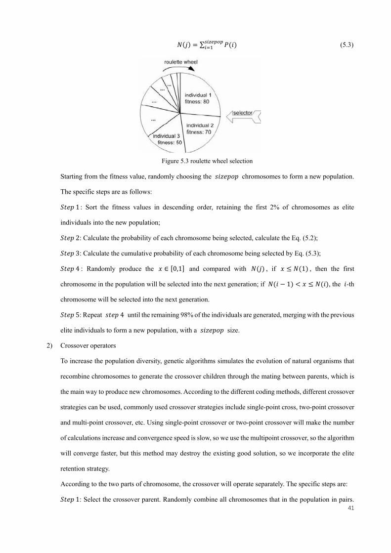
41
𝑁(𝑗) = ∑ 𝑃(𝑖)𝑠𝑖𝑧𝑒𝑝𝑜𝑝𝑖=1 (5.3)
Figure 5.3 roulette wheel selection
Starting from the fitness value, randomly choosing the 𝑠𝑖𝑧𝑒𝑝𝑜𝑝 chromosomes to form a new population.
The specific steps are as follows:
𝑆𝑡𝑒𝑝 1 : Sort the fitness values in descending order, retaining the first 2% of chromosomes as elite
individuals into the new population;
𝑆𝑡𝑒𝑝 2: Calculate the probability of each chromosome being selected, calculate the Eq. (5.2);
𝑆𝑡𝑒𝑝 3: Calculate the cumulative probability of each chromosome being selected by Eq. (5.3);
𝑆𝑡𝑒𝑝 4 : Randomly produce the 𝑥 ∈ [0,1] and compared with 𝑁(𝑗) , if 𝑥 ≤ 𝑁(1) , then the first
chromosome in the population will be selected into the next generation; if 𝑁(𝑖 − 1) < 𝑥 ≤ 𝑁(𝑖), the 𝑖-th
chromosome will be selected into the next generation.
𝑆𝑡𝑒𝑝 5: Repeat 𝑠𝑡𝑒𝑝 4 until the remaining 98% of the individuals are generated, merging with the previous
elite individuals to form a new population, with a 𝑠𝑖𝑧𝑒𝑝𝑜𝑝 size.
2) Crossover operators
To increase the population diversity, genetic algorithms simulates the evolution of natural organisms that
recombine chromosomes to generate the crossover children through the mating between parents, which is
the main way to produce new chromosomes. According to the different coding methods, different crossover
strategies can be used, commonly used crossover strategies include single-point cross, two-point crossover
and multi-point crossover, etc. Using single-point crossover or two-point crossover will make the number
of calculations increase and convergence speed is slow, so we use the multipoint crossover, so the algorithm
will converge faster, but this method may destroy the existing good solution, so we incorporate the elite
retention strategy.
According to the two parts of chromosome, the crossover will operate separately. The specific steps are:
𝑆𝑡𝑒𝑝 1: Select the crossover parent. Randomly combine all chromosomes that in the population in pairs.

42
Form [𝑠𝑖𝑧𝑒𝑝𝑜𝑝
2⁄ ] sets of parents, choose one set inside [𝑠𝑖𝑧𝑒𝑝𝑜𝑝
2⁄ ] to crossover;
𝑆𝑡𝑒𝑝 2: Randomly generate 𝑥 ∈ [0,1], compared with 𝑃𝑐 (crossover probability, generally < 1), if 𝑥 ≤
𝑃𝑐, implement the multi-point crossover. The specific processes are:
①. Remove all 0 genes in the driving route (inside the first part) of the parent chromosome, and record
the locations of these 0 genes;
②. In the range[1, 𝑁 + 𝑀] randomly generate 𝑚 numbers as crossover points;
③. Exchange the genes at the intersection of the two parent chromosomes;
④. Test respectively the repeated genes in the children and replace them with the missing genes. The
sequence is consistent with the gene sequence in the middle of the original chromosome intersection.
⑤. Add the 0 genes at the recorded positions.
We illustrate the process of coding and decoding by using 10 customer points, 3 charging stations and 3 EVs.
So, 𝑁 = 10, 𝑀 = 3 , the crossover points 𝑚 = 3 . The first part of two parent chromosomes are
(0,5,3,13,1,0,8,4,11,9,2,0,10,6,12,7,0) and (0,6,3,0,11,7,10,8,5,12,1,2,0,4,9,13,0) . The first parent
chromosome randomly generate 3 crossover points are (2,4,11), the second parent chromosome’s crossover
points are (1,4,7) , the two children obtained by crossover are (0,5,6,13,7,0,8,4,11,9,2,0,10,1,12,3,0) and
(0,3,5,0,11,10,8,6,12,7,2,0,4,9,13,0).
The crossover method of the second part (charging station locations) is similar with the first part, the only
difference is that there is no need to remove the 0 gene position, but directly crossover. For example, the two
parent chromosomes’ second parts are (1,0,1) and (0,0,1), the crossover point generated randomly are both at
1. So the complete chromosomes after crossover are (0,5,6,13,7,0,8,4,11,9,2,0,10,1,12,3,0,0,0,1) and
(0,3,5,0,11,10,8,6,12,7,2,0,4,9,13,0,1,0,1). The complete crossover process is shown in Figure 5.4:
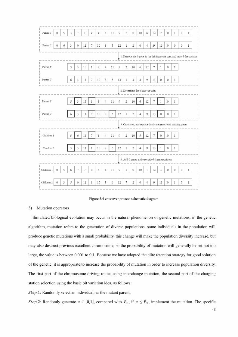
43
Figure 5.4 crossover process schematic diagram
3) Mutation operators
Simulated biological evolution may occur in the natural phenomenon of genetic mutations, in the genetic
algorithm, mutation refers to the generation of diverse populations, some individuals in the population will
produce genetic mutations with a small probability, this change will make the population diversity increase, but
may also destruct previous excellent chromosome, so the probability of mutation will generally be set not too
large, the value is between 0.001 to 0.1. Because we have adopted the elite retention strategy for good solution
of the genetic, it is appropriate to increase the probability of mutation in order to increase population diversity.
The first part of the chromosome driving routes using interchange mutation, the second part of the charging
station selection using the basic bit variation idea, as follows:
𝑆𝑡𝑒𝑝 1: Randomly select an individual, as the mutant parent;
𝑆𝑡𝑒𝑝 2: Randomly generate 𝑥 ∈ [0,1], compared with 𝑃𝑚, if 𝑥 ≤ 𝑃𝑚, implement the mutation. The specific
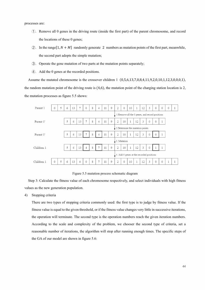
44
processes are:
①. Remove all 0 genes in the driving route (inside the first part) of the parent chromosome, and record
the locations of these 0 genes;
②. In the range[1, 𝑁 + 𝑀] randomly generate 2 numbers as mutation points of the first part, meanwhile,
the second part adopts the simple mutation;
③. Operate the gene mutation of two parts at the mutation points separately;
④. Add the 0 genes at the recorded positions.
Assume the mutated chromosome is the crossover children 1 (0,5,6,13,7,0,8,4,11,9,2,0,10,1,12,3,0,0,0,1),
the random mutation point of the driving route is (4,6), the mutation point of the charging station location is 2,
the mutation processes as figure 5.5 shows:
Figure 5.5 mutation process schematic diagram
Step 3: Calculate the fitness value of each chromosome respectively, and select individuals with high fitness
values as the new generation population.
4) Stopping criteria
There are two types of stopping criteria commonly used: the first type is to judge by fitness value. If the
fitness value is equal to the given threshold, or if the fitness value changes very little in successive iterations,
the operation will terminate. The second type is the operation numbers reach the given iteration numbers.
According to the scale and complexity of the problem, we chooser the second type of criteria, set a
reasonable number of iterations, the algorithm will stop after running enough times. The specific steps of
the GA of our model are shown in figure 5.6:

45
Figure 5.6 GA flowchart

46
6. Case analysis
The vehicles used for urban distribution are traditional fuel vehicles and EFVs, at present, fossil fuel vehicles
are still the main distribution method, with a market share of 98% in China [27]. While, the characteristics of zero
pollution and low energy consumption of EFVs have made it popular in recent years. In order to confirm the
accuracy and effectiveness of the electric vehicles LRP model and genetic algorithm proposed in this thesis, this
section will use medium and large-scale cases to verify the model.
6.1 Algorithm implementation
All calculation cases are performed on the computer: Intel (R) Core (TM) i7-8550U CPU @ 1.80GHz, 8GB
RAM, Windows 10 operation system. Genetic algorithm codes are implemented on the MATLAB R2020a.
In the coding process, I think the most difficult point is the design of the crossover process. the routes part
and the charging station selection part are crossover separately, then duplicate parts are eliminated, the detailed
process is as follows:
Crossover process codes
S1: if rand (1) < pcross
generate randomly 𝑥 ∈ [0,1], compared with 𝑃𝑐, if 𝑥 ≤ 𝑃𝑐, implement the multi-point crossover
S2: ppc1 = pcross1(1: length(pcross1)-Nstation);
ppc2 = pcross2 (1: length(pcross1)-Nstation);
Remove the 0 genes in the routes part (first part)
zeropos1= find(ppc1==0);
ppc1 (zeropos1) = [];
zeropos2= find(ppc2==0);
ppc2 (zeropos2) = [];
Record all the positions of 0 genes, for later recovery
S3: generate randomly 3 numbers ∈ [1, 𝑁 + 𝑀] as the crossover points
crosspos1 = sort(randperm(length(pop1),3),'ascend');
crosspos2 = sort(randperm(length(pop1),3),'ascend');
S4: exchange the genes at each crossover point of the two parents, keep one of the genes as the output of cross
p1cross(crosspos1) = p2cross(crosspos2);
p2cross(crosspos2) = ptemp(crosspos1);
S5: separately check the repeated genes in the children
ptime = setdiff(pop1, p1cross); postime = zeros(1,length(ptime));
for i = 1: length (ptime)
postime(i) = find(pop1==ptime(i));
end
Replace the repeated genes with the missing genes, the sequence is same with the gene sequence in the middle
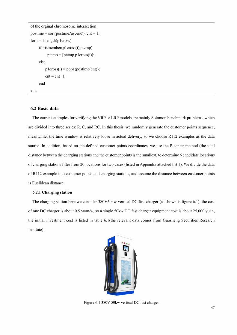
47
of the orginal chromosome intersection
postime = sort(postime,'ascend'); cnt = 1;
for i = 1:length(p1cross)
if ~ismember(p1cross(i),ptemp)
ptemp = [ptemp,p1cross(i)];
else
p1cross(i) = pop1(postime(cnt));
cnt = cnt+1;
end
end
6.2 Basic data
The current examples for verifying the VRP or LRP models are mainly Solomon benchmark problems, which
are divided into three series: R, C, and RC. In this thesis, we randomly generate the customer points sequence,
meanwhile, the time window is relatively loose in actual delivery, so we choose R112 examples as the data
source. In addition, based on the defined customer points coordinates, we use the P-center method (the total
distance between the charging stations and the customer points is the smallest) to determine 6 candidate locations
of charging stations filter from 20 locations for two cases (listed in Appendix attached list 1). We divide the data
of R112 example into customer points and charging stations, and assume the distance between customer points
is Euclidean distance.
6.2.1 Charging station
The charging station here we consider 380V50kw vertical DC fast charger (as shown is figure 6.1), the cost
of one DC charger is about 0.5 yuan/w, so a single 50kw DC fast charger equipment cost is about 25,000 yuan,
the initial investment cost is listed in table 6.1(the relevant data comes from Guosheng Securities Research
Institute):
Figure 6.1 380V 50kw vertical DC fast charger

48
Single 50kw DC charger investment cost
Total cost Charging equipment + power distribution equipment
+ civil construction cost
57,000-60,000
Charging equipment cost Contains monitoring, charger module, assemblies
box, relay, etc.
25,000
Civil construction cost Building operations, electric wire, etc. 10,000-13,000
Power distribution equipment cost low-voltage apparatus, electricity meter, etc. 22,000
Table 6.1 single DC fast charger investment cost
Consider the slow charger is cheap, and the investment in civil engineering and power distribution equipment
is less, assuming that the investment of one slow charger is 0.5 yuan/w, the total investment cost of one fast
charger is calculated as 1.2 yuan/w. Suppose the equipment depreciation period is 10 years, the average annual
maintenance cost is 3% of the initial investment, and the average annual operating and labor costs are 6% of the
initial investment. The average annual fixed cost is listed in table 6.2:
Costs 7.5kw 50kw
Single charger initial investment 4000 60,000
Annual depreciation expense (10 years) 400 6,000
Annual equipment maintenance cost 100 1,800
Average annual operating labor cost per pile 200 3,600
Total annual fixed expenses (regardless of venue) 700 11,400
Table 6.2 average annual fixed cost per one DC charger pile
6.2.2 Vehicle relevant parameters
The basic parameter settings of EFVs refer to the configuration parameters of Nissan e-NV200 (Figure 6.2),
specific parameters listed in table 6.3, other parameters are shown in table 6.4 (the relevant data comes from
Guosheng Securities Research Institute):
Figure 6.2 Nissan e-NV200

49
Parameters Values
Maximum loading capacity 700kg
Maximum mileage 200km
Battery capacity 40kwh
Vehicle speed 30km/h
Consumption of battery per km 0.143kwh/km
Charging factor 60kwh/h
Table 6.3 e-NV 200 configuration parameters
Parameters Values Service time for one customer 10 mins Electric conversion coefficient 0.94 Electricity fee 0.55 yuan/kwh Minimum safe battery percent 20% Fixed cost 100 yuan/vehicle Transport cost 2 yuan/km Carbon emission price 0.5 yuan/kg Waiting cost for vehicle arriving early 1 yuan/mins Penalty cost for vehicle arriving late 2 yuan/mins
Table 6.4 other parameters
As comparison, the traditional fuel vehicle’s basic parameter refers to the Nissan NV 200 (Figure 6.3, same
model as electric vehicle), relevant parameters list in table 6.5:
Figure 6.3 Nissan NV 200
Parameters Values
Engine 1.6 L
Maximum load capacity 700 kg
Fuel consumption 0.07 L/km
Carbon emission per unit liter of gasoline 2.3 kg/L
Oil price 6.13 yuan /L
Table 6.5 NV 200 parameters
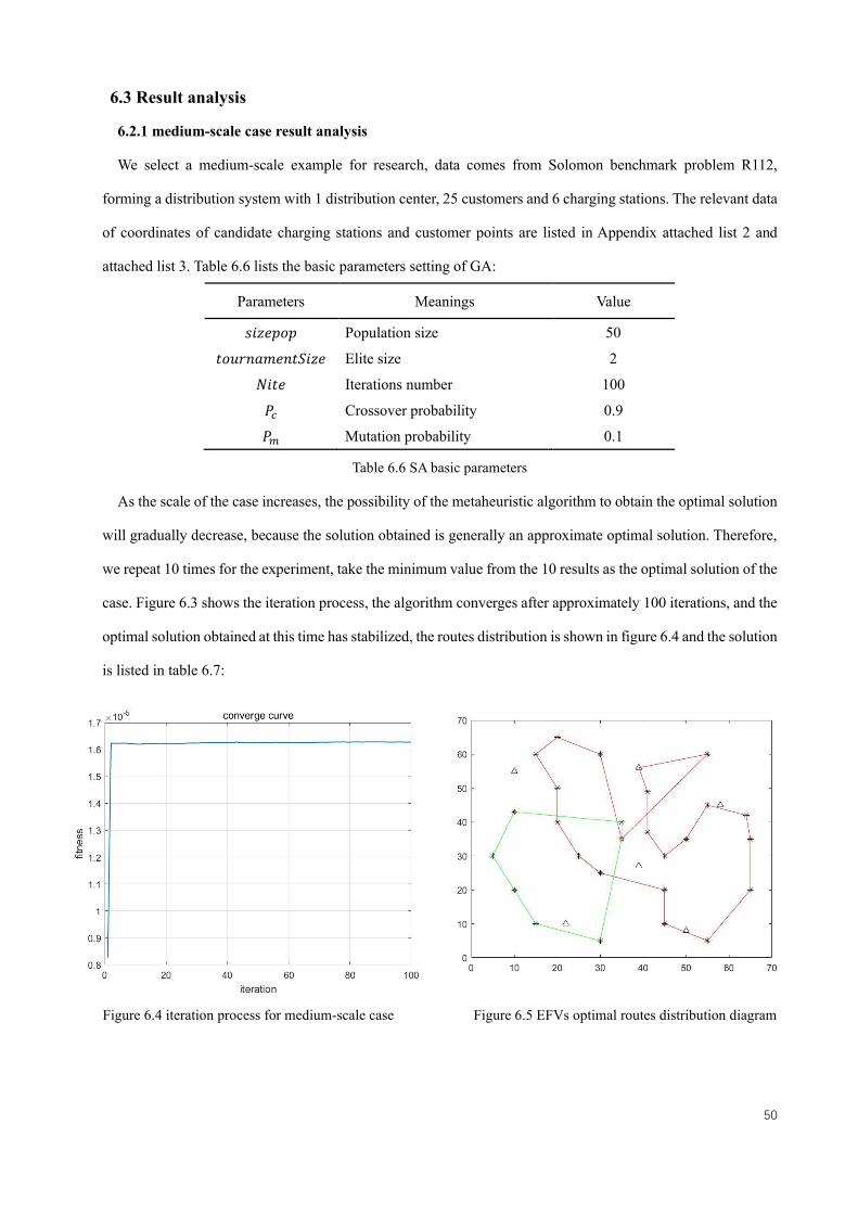
50
6.3 Result analysis
6.2.1 medium-scale case result analysis
We select a medium-scale example for research, data comes from Solomon benchmark problem R112,
forming a distribution system with 1 distribution center, 25 customers and 6 charging stations. The relevant data
of coordinates of candidate charging stations and customer points are listed in Appendix attached list 2 and
attached list 3. Table 6.6 lists the basic parameters setting of GA:
Parameters Meanings Value
𝑠𝑖𝑧𝑒𝑝𝑜𝑝 Population size 50
𝑡𝑜𝑢𝑟𝑛𝑎𝑚𝑒𝑛𝑡𝑆𝑖𝑧𝑒 Elite size 2
𝑁𝑖𝑡𝑒 Iterations number 100
𝑃𝑐 Crossover probability 0.9
𝑃𝑚 Mutation probability 0.1
Table 6.6 SA basic parameters
As the scale of the case increases, the possibility of the metaheuristic algorithm to obtain the optimal solution
will gradually decrease, because the solution obtained is generally an approximate optimal solution. Therefore,
we repeat 10 times for the experiment, take the minimum value from the 10 results as the optimal solution of the
case. Figure 6.3 shows the iteration process, the algorithm converges after approximately 100 iterations, and the
optimal solution obtained at this time has stabilized, the routes distribution is shown in figure 6.4 and the solution
is listed in table 6.7:
Figure 6.4 iteration process for medium-scale case Figure 6.5 EFVs optimal routes distribution diagram

51
Indicators Values
Optimal solution 60837.88 yuan
Optimal distribution cost
(without CS cost)
837.88 yuan
Routes ⚫ 0--7--8--16--4--15--3--10--17--18--19--21--20--25--
2--9--22--24--1--29(charging)--6 (red line)
⚫ 0--23--5--14--13--11--12--0 (green line)
Fixed cost 200 yuan
Transport cost 592.27 yuan (296.14 km)
Charging cost 16.30 yuan
Environment cost 14.45 yuan
Penalty cost 14.86 yuan
Table 6.7 Results of calculation case
According to figure 6.5 and table 6.7, in the given 4 alternative charging stations, No.29 node, coordinate
(58,45), is chosen to build a charging station. Besides, in order to verify the stability of the algorithm, we run
the calculation examples 10 times, obtain the 10 optimal solution for each time and calculate the deviation value,
as shown in table 6.8:
Time Optimal value Deviation value
1 60850.21 0.02%
2 60837.88 --
3 60861.31 0.04%
4 60842.10 0.01%
5 60911.32 0.12%
6 60892.80 0.09%
7 60945.82 0.18%
8 60946.56 0.18%
9 60851.65 0.02%
10 60874.28 0.06%
Average 60881.39 0.07%
Table 6.8 calculation examples results of 10 run times
In 10 run times, the average value of the solution is 60881.39, and the average deviation of the solution is
0.07%. During operation, appears 1 optimal solution – 60837.88, and all solutions deviation are controlled within
1%, and the maximum deviation is 0.18%. As a whole, we can see that the quality of the solutions obtained in

52
10 run times is good, the deviations are all within a reasonable range, indicating that the genetic algorithm model
is stable.
Then we compare the result of EFVs distribution with traditional fuel vehicle. For the convenience of
comparison, consider the traditional fuel vehicles costs contain: fixed cost, transportation cost, fuel cost,
environmental cost and time window penalty cost. The calculation examples used is same with EFVs case. The
experiment is repeated 10 times, and the optimal solution is the minimum value in the 10 results, the optimal
path is shown in the figure 6.7:
Figure 6.6 fuel vehicle optimal routes distribution diagram
Compare the solution results of fuel vehicle distribution with the results of EFVs distribution, the comparison
items are listed in table 6.9:
Indicators Electric freight vehicle Traditional fuel vehicle
Optimal solution (without CS cost) 837.88 yuan 939.81 yuan
CS construction cost 60,000yuan --
Fixed cost 200 yuan 200 yuan
Transport cost 592.27 yuan (296.14 km) 565.34 yuan (282.67km)
Charging cost/fuel cost 16.30 yuan 121.29 yuan
Environmental cost 14.45 yuan 41.26 yuan
Time window penalty cost 14.86 yuan 11.92 yuan
Distribution routes ⚫ 0--7--8--16--4--15--3--10--17--18--
19--21--20--25--2--9--22--24--1--
29(charging)--6 (red line)
⚫ 0--17--18--19--21--20--25--2--9--
22--24--23--0 (red line)

53
⚫ 0--23--5--14--13--11--12--0 (green
line)
⚫ 0--6--7--8--16--4--15--5--14--13--
11--12--10--3--1--0 (green line)
Table 6.9 results comparison of EFVs and fuel vehicles
From the above table, we can know that for one mission, the distribution cost of using EFVs (excluding
charging station relevant costs) is less than that using fuel vehicles, so if we use EFVs for distribution, we can
pay less 101.93 yuan for each mission, save an average of 0.36 yuan/km. Because the needs for battery
replenishment during delivery, the transportation distance and cost are higher than that of fuel vehicles, the
exceed cost is16.93 yuan. The time window penalty cost of using EFVs is a little larger than that of fuel vehicles.
While, the charging cost is significantly lower than the fuel cost of fuel vehicle, only account for 13.4% of fuel
cost, and carbon emission costs are also reduced by 65%. Therefore, from the perspective of economic and
environmental benefits, EFVs have obvious advantages.
Then, we consider the total cost (plus charging station relevant costs), from section 6.2.1, we know that:
1) One 7.5kw slow charger investment cost is 4000 yuan, the average annual fixed cost is 700 yuan, logistics
company should have slow charging facilities in order to charging EFVs at night to save charging costs,
here we consider one 7.5kw slow charger in DC;
2) One 50kw DC fast charger investment cost is about 60,000 yuan and the average annual fixed cost is 11,400
yuan, the upfront investment in self-built charging station is huge, we build one DC fast charger at point
(39,56).
Suppose vehicles drive 300 days a year, and one distribution mission per day. The distribution cost is 837.88
yuan/mission for using EFVs and 939.81 yuan/mission for using traditional fuel vehicles, the distribution cost
saved by using EFVs is 30,579 yuan/year. The total annual cumulative cost is shown in figure 6.7:
Figure 6.7 comparison of total logistics cumulative cost between EFVs and traditional fuel vehicles
0 1 2 3 4 5 6 7 8 9 10
EFVs 64,000 327,464 590,928 854,392 1,117,856 1,381,320 1,644,784 1,908,248 2,171,712 2,435,176 2,698,640
Fuel vehicles 0 281,943 563,886 845,829 1,127,772 1,409,715 1,691,658 1,973,601 2,255,544 2,537,487 2,819,430
0
500,000
1,000,000
1,500,000
2,000,000
2,500,000
3,000,000
EFVs Fuel vehicles

54
From the above figure, we can see that starting from the 4th year, the total logistics cost of using EFVs has
become less than that of using fuel vehicles. In other words, at least 4 years before investors can actually earn a
profit. Until the 10th year of using EFVs, the logistic company can save 120,790 yuan (≈15,098 euro) totally in
distribution cost, the total cost saved is not much, so in this medium-scale case of customer demand, the self-
built charging station mode of company cannot bring huge benefits. Company is profitable because the annual
cost savings by using EFVs distribution is larger than the annual cost of the charging stations, all costs of the
charging station are borne by logistics company, the utilization rate of the charging station is low, so the charging
station is always operating at a loss, especially the high cost of fast charging station, the total investment payback
period is long.
If the fast charging station we build can be used publicly or shared with other logistics companies, then the
charging station operation can be profitable, and the total investment payback period of logistics company will
also be accelerated. At present, the most basic profit method for charging stations is collect charging electricity
and service fees. We consider the charging service fee is 0.55 yuan/kw, charging station operates 330 days a year,
if the utilization rate of a single 50kw DC fast charger is 7% (1.68 hours per day), the payback period of
investment will take 15.6 years, if the utilization rate increase to 30% (8 hours per day), the payback period will
be 0.98 years, table 6.10 lists payback period under different utilization rates:
Utilization rate 7% 10% 15% 20% 30% 50%
Hours/day 1.68 2.4 3.6 4.8 7.2 12
Payback period (years) 15.60 5.78 2.82 1.87 1.11 0.62
Table 6.10 payback period under different utilization rates
From the above table, we can know that the payback period of single charger is greatly affected by the
utilization rate (= annual accumulated charging time / total time of a year). For example: if the fast charging
station can be used for EFVs belongs to other logistics companies, during the 300 delivery times for a year, the
utilization rate is 10%, the charging station daily service EFVs number is 4 (including 3 EFVs from other
companies), then the company will be profitable in the 1.9th year. We can see the payback period is much shorter
than before, and at the 10th year, the logistic company can save 269,290 yuan totally in total cost, around 2.2
times as before.
6.2.2 large-scale case result analysis
The large-scale example uses the 61 nodes in the Solomon benchmark problem R112, forming a distribution
system with 1 distribution center, 60 customers and 6 alternative charging stations. The relevant data of

55
coordinates of charging stations and customer points are shown in Appendix attached list 2 and attached list 4.
Table 6.11 lists the basic parameters setting of genetic algorithms:
Parameters Meanings Value
𝑠𝑖𝑧𝑒𝑝𝑜𝑝 Population size 100
𝑡𝑜𝑢𝑟𝑛𝑎𝑚𝑒𝑛𝑡𝑆𝑖𝑧𝑒 Elite size 2
𝑁𝑖𝑡𝑒 Iterations number 150
𝑃𝑐 Crossover probability 0.9
𝑃𝑚 Mutation probability 0.1
Table 6.11 GA basic parameters
Figure 6.8 iteration process for large-scale case
Figure 6.8 shows the iteration process of using EFVs to distribution, the algorithm converges after
approximately 150 iterations, and the optimal solution obtained at this time has stabilized, the routes distribution
is shown in figure 6.9 and the solution is listed in table 6.12:
Figure 6.9 EFVs optimal routes distribution diagram

56
Indicators Values
Optimal solution 181799.44 yuan
Optimum distribution
cost (without CS cost)
1799.44 yuan
Charging station cost 60,000 yuan × 3
Routes ⚫ 0--52--18--60--5--59--37--42--57--2--40--58--53--1--30--0 (red line)
⚫ 0--41--15--22--23--55--39--56--25--24--29--34--33--51--66(charging)--3--9--35--0 (green
line)
⚫ 0--11--7--48--47--36--49--19--46--8--45--17--16--44--14--38--61(charging)--6--27--0
(black line)
⚫ 0--43--13--26--21--4--54--12--28--50--10--31--64(charging)--32--20--0 (yellow line)
Fixed cost 400 yuan
Transport cost 1270.18 yuan (635.09 km)
Charging cost 51.76 yuan
Environment cost 30.48 yuan
Penalty cost 47.02 yuan
Table 6.12 Results of calculation case
According to figure 6.9 and table 6.12, in the given 6 alternative charging stations, No.61,64 and 66 nodes,
coordinate (22,10), (39,56) and (58,45), are chosen to build charging stations. Besides, in order to verify the
stability of the algorithm, we run the calculation examples 10 times, obtain the 10 optimal solution for each time
and calculate the deviation value, as shown in table 6.13:
Time Optimal value Deviation value
1 181932.70 0.07%
2 181970.85 0.09%
3 182023.40 0.12%
4 181830.93 0.02%
5 181837.25 0.02%
6 181799.44 --
7 181859.62 0.03%
8 182009.60 0.12%
9 182184.29 0.21%
10 181946.76 0.08%
Average 181939.48 0.07%
Table 6.13 calculation examples results of 10 run times
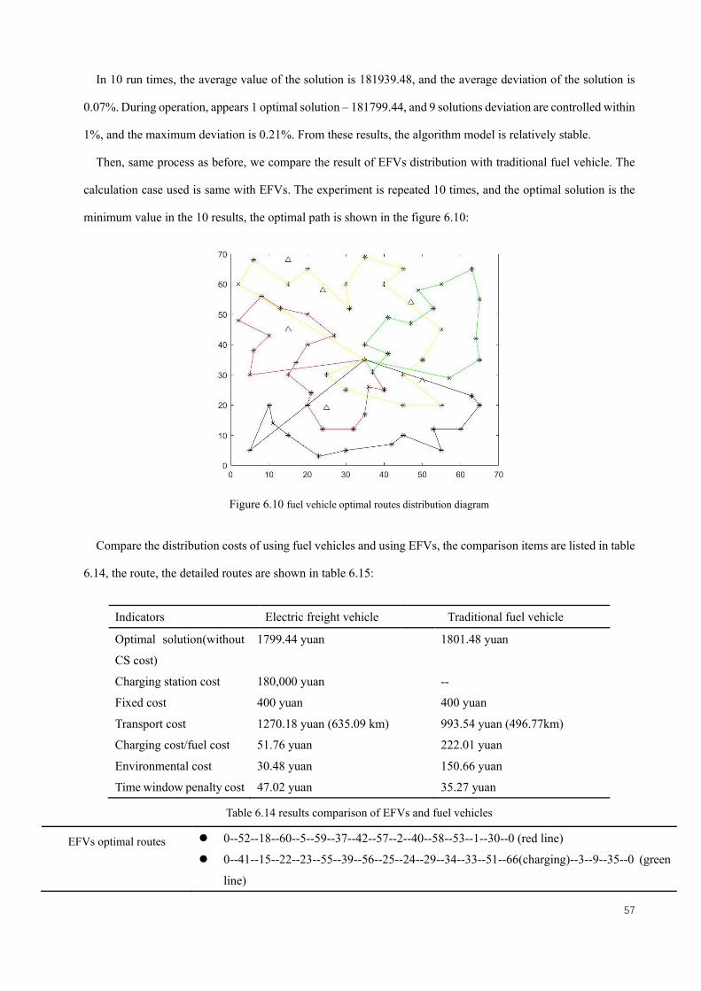
57
In 10 run times, the average value of the solution is 181939.48, and the average deviation of the solution is
0.07%. During operation, appears 1 optimal solution – 181799.44, and 9 solutions deviation are controlled within
1%, and the maximum deviation is 0.21%. From these results, the algorithm model is relatively stable.
Then, same process as before, we compare the result of EFVs distribution with traditional fuel vehicle. The
calculation case used is same with EFVs. The experiment is repeated 10 times, and the optimal solution is the
minimum value in the 10 results, the optimal path is shown in the figure 6.10:
Figure 6.10 fuel vehicle optimal routes distribution diagram
Compare the distribution costs of using fuel vehicles and using EFVs, the comparison items are listed in table
6.14, the route, the detailed routes are shown in table 6.15:
Indicators Electric freight vehicle Traditional fuel vehicle
Optimal solution(without
CS cost)
1799.44 yuan 1801.48 yuan
Charging station cost 180,000 yuan --
Fixed cost 400 yuan 400 yuan
Transport cost 1270.18 yuan (635.09 km) 993.54 yuan (496.77km)
Charging cost/fuel cost 51.76 yuan 222.01 yuan
Environmental cost 30.48 yuan 150.66 yuan
Time window penalty cost 47.02 yuan 35.27 yuan
Table 6.14 results comparison of EFVs and fuel vehicles
EFVs optimal routes ⚫ 0--52--18--60--5--59--37--42--57--2--40--58--53--1--30--0 (red line)
⚫ 0--41--15--22--23--55--39--56--25--24--29--34--33--51--66(charging)--3--9--35--0 (green
line)

58
⚫ 0--11--7--48--47--36--49--19--46--8--45--17--16--44--14--38--61(charging)--6--27--0
(black line)
⚫ 0--43--13--26--21--4--54--12--28--50--10--31--64(charging)--32--20--0 (yellow line)
Fuel vehicles optimal routes ⚫ 0--17--45--8--46--47--48--7--52--18--60--5--59--37--42--57--2--58--40--0 (red line)
⚫ 0--53--28--27--1--50--33--51--9--35--34--29--24--54--0 (green line)
⚫ 0--55--25--39--56--23--22--41--15--43--14--44--16--38--0 (black line)
⚫ 0--6--13--21--4--26--12--3--30--20--32--10--31--11--19--49--36--0 (yellow line)
Table 6.15 optimal distribution routes comparison
From the feasible solution obtained in the above tables, it can be seen that in the large-scale case (long-
distance transportation process), the use of EFVs distribution and the use of traditional fuel vehicle distribution
required costs are not much different, the difference value is only 2.04 yuan for each mission. Meanwhile, EFVs
need to be charged in the distribution process, resulting in transportation cost (distance) and time window penalty
cost are higher than the use of traditional fuel vehicle distribution. But the EFVs’ charging costs and
environmental costs are much lower than the fuel vehicles, where the environmental cost reduced by 79.77%,
Therefore, the total cost of using EFVs for the same mission almost same with using fuel vehicles.
Then, consider we should build 3 charging stations (50kw DC fast charger) in this large-scale case, the
initial investment is 180,000 yuan, average annual fixed cost increasing 34,200 yuan. The distribution cost saved
by using EFVs is 2.04yuan/mission. In this large-scale case, self-built charging station of company have no
benefits. Same as before, we consider the 3 charging stations available for the EFVs of other logistics companies,
under the same assumptions as previous, if the utilization rate of each charging station is 10%, each charging
station daily service EFVs number is 4 (including 3 EFVs from other companies), then the company will be
profitable in the 7th year, much longer than before. If the utilization rate is 20%, it means each charging station
daily service EFVs number is around 8, then the company will be profitable in the middle of the 1st year. The
key is to increase the utilization rate of charging stations, reasonably open charging stations for public.
6.4 Conclusions
This thesis integrates the charging station cost, charging cost and environmental cost into the electric vehicle
LRP model, and designs the genetic algorithm to solve the model, so some corresponding conclusions are drawn.
According to the two scale of examples, Table 6.16 lists the saved cost of using EFVs with respect of fuel
vehicles:
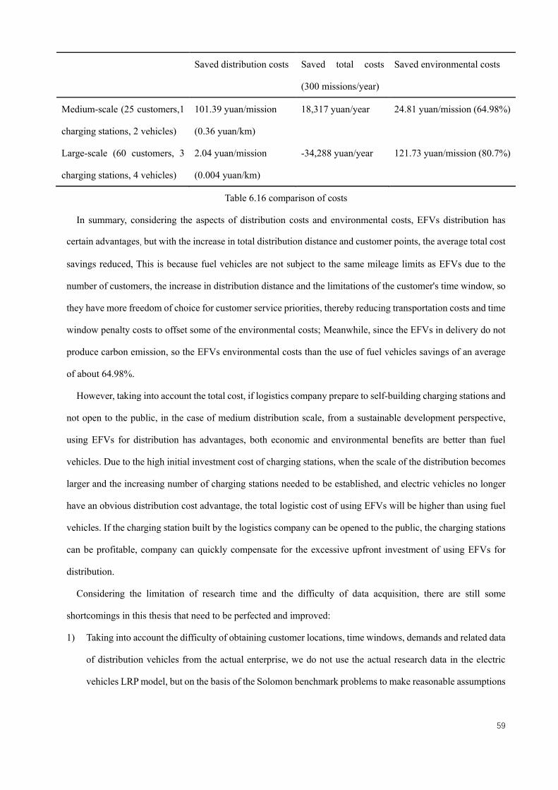
59
Saved distribution costs Saved total costs
(300 missions/year)
Saved environmental costs
Medium-scale (25 customers,1
charging stations, 2 vehicles)
101.39 yuan/mission
(0.36 yuan/km)
18,317 yuan/year 24.81 yuan/mission (64.98%)
Large-scale (60 customers, 3
charging stations, 4 vehicles)
2.04 yuan/mission
(0.004 yuan/km)
-34,288 yuan/year 121.73 yuan/mission (80.7%)
Table 6.16 comparison of costs
In summary, considering the aspects of distribution costs and environmental costs, EFVs distribution has
certain advantages, but with the increase in total distribution distance and customer points, the average total cost
savings reduced, This is because fuel vehicles are not subject to the same mileage limits as EFVs due to the
number of customers, the increase in distribution distance and the limitations of the customer's time window, so
they have more freedom of choice for customer service priorities, thereby reducing transportation costs and time
window penalty costs to offset some of the environmental costs; Meanwhile, since the EFVs in delivery do not
produce carbon emission, so the EFVs environmental costs than the use of fuel vehicles savings of an average
of about 64.98%.
However, taking into account the total cost, if logistics company prepare to self-building charging stations and
not open to the public, in the case of medium distribution scale, from a sustainable development perspective,
using EFVs for distribution has advantages, both economic and environmental benefits are better than fuel
vehicles. Due to the high initial investment cost of charging stations, when the scale of the distribution becomes
larger and the increasing number of charging stations needed to be established, and electric vehicles no longer
have an obvious distribution cost advantage, the total logistic cost of using EFVs will be higher than using fuel
vehicles. If the charging station built by the logistics company can be opened to the public, the charging stations
can be profitable, company can quickly compensate for the excessive upfront investment of using EFVs for
distribution.
Considering the limitation of research time and the difficulty of data acquisition, there are still some
shortcomings in this thesis that need to be perfected and improved:
1) Taking into account the difficulty of obtaining customer locations, time windows, demands and related data
of distribution vehicles from the actual enterprise, we do not use the actual research data in the electric
vehicles LRP model, but on the basis of the Solomon benchmark problems to make reasonable assumptions
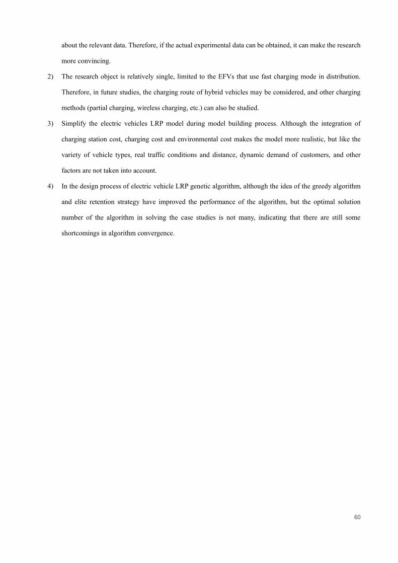
60
about the relevant data. Therefore, if the actual experimental data can be obtained, it can make the research
more convincing.
2) The research object is relatively single, limited to the EFVs that use fast charging mode in distribution.
Therefore, in future studies, the charging route of hybrid vehicles may be considered, and other charging
methods (partial charging, wireless charging, etc.) can also be studied.
3) Simplify the electric vehicles LRP model during model building process. Although the integration of
charging station cost, charging cost and environmental cost makes the model more realistic, but like the
variety of vehicle types, real traffic conditions and distance, dynamic demand of customers, and other
factors are not taken into account.
4) In the design process of electric vehicle LRP genetic algorithm, although the idea of the greedy algorithm
and elite retention strategy have improved the performance of the algorithm, but the optimal solution
number of the algorithm in solving the case studies is not many, indicating that there are still some
shortcomings in algorithm convergence.

61
REFERENCES
[1] Lin H. Optimization of the urban vehicle routing problem of pure electric vehicles. Chang’an university,
2018.
[2] Wang Y C. The vehicle routing problem research of urban freight distribution based on electric vehicles.
Beijing jiaotong university, 2012.
[3] Wang H, Shen J. Heuristic approaches for solving transit vehicle scheduling problem with route and fueling
time constraints. Applied Mathematics and Computation, 2007, 190(2).
[4] Fincher, Marcelo. 5 Ways to Overcome Last Mile Delivery Challenges, 2017.
[5] Zhang L. Research on operation organization optimization of urban distribution electric logistics vehicle
based on FBSM. Beijing jiaotong university, 2019.
[6] China’s logistics service industry report, iReserach, 2019.
[7] Li D G, Discrimination of green logistics and low-carbon logistics. China storage and transportation, 2010.
[8] Zhou H C. Development of carbon market in the world and its implications. China soft science, 2009.
[9] Yang N. Research on the optimization of vehicle routing problem of urban express delivery considering
carbon emission. Beijing university of posts and telecommunications, 2018.
[10] Philippe Lebeau, Cathy Macharis, Joeri van mierlo. Exploring the choice of battery electric vehicles in city
logistics: A conjoint-based choice analysis. Vrije university Brussel, 2015.
[11] Dale Hall, Cui H Y, Nic Lustey. Electric vehicle capitals: showing the path to a mainstream market. ICCT,
2019.
[12] Li S Q. Research on the location-routing problem of electric vehicles in logistics distribution system. North
China Electric Power University, 2018.
[13] Zhang G L. Research on the Location Problem of Electric Vehicle Charging Station Intra-city and Inter-city.
Tianjing University, 2012.
[14] Yang Q. Research on charging station location-routing problem of electric logistics vehicles. Chang’an
university, 2019.
[15] Ma Y H. Research on urban collaborative logistics distribution model and application based on electric
logistics vehicle. Beijing jiaotong university, 2018.
[16] Hans Quak, Nina Nesterova. Zero emission city logistics: current practices in freight electromobility and
feasibility in the near future. 6th Transport Research Arena April 18-21, 2016.
[17] Xi Y. New energy vehicles help green logistics development. China Logistics and Purchasing issue 8, 2018.

62
[18] Zhang Q Y. Research on LRP optimization of electric vehicle logistics distribution in Beijing-Tianjin-Hebei
regione. North China Electric Power University, 2019.
[19] Qi E. Logistic engineering. China Science and Technology Press, 2004:160-165.
[20] Drexl M, Schneider M. A survey of variants and extensions of the location-routing problem. European
Journal of Operational Research, 2015.
[21] Luo J Y. Improved binary particle swarm optimization algorithm for vehicle routing problem. The Practice
and Understanding of Mathmatics, 2014.
[22] Geng X. An Improvement to Table-Working Method and Its Application to Approximate Supply and
Demand Balancing Problems. Shandong Normal University, 2012.
[23] Li X L, Shao Z J. An optimizing method based on autonomous animates: Fish swarm algorithm. Zhejiang
University, 2002.
[24] Holland J H. Adaptation in Natural and Artificial Systems. Ann Arbor: University of Michigan Press, 1975.
[25] Lei Y J. Matlab genetic algorithm toolbox and application. Xi'an University of Electronic Science and
Technology Press, 2005.
[26] Ding L F, Zhi W. Simulation Research on the Selection of Control Parameters of Genetic Algorithm. Science
and Technology Information, 2007.
[27] Wu S H. Research on Optimization of Urban Distribution Scheduling for Pure Electric Logistics Vehicles.
Beijing jiaotong university, 2018.

63
APPENDIX Attached list 1 coordinates where charging stations can be built
Number 𝑥 coordinate 𝑦 coordinate
1 4 14 2 22 10 3 50 8 4 62 23 5 39 27 6 28 35 7 4 37 8 35 17 9 55 20 10 15 30 11 31 52 12 46 39 13 39 56 14 65 61 15 10 55 16 58 45 17 25 19 18 24 58 19 15 45 20 18 68
Attached list 2 charging station coordinates
number x coordinate y coordinate 1 22 10 2 50 8 3 39 27 4 39 56 5 10 55 6 58 45
Attached list 3 medium-scale case: customer points data
Number 𝑥 coordinate 𝑦 coordinate Demand Starting time Ending time
0 35 35 0 0 8 1 41 49 46 2.4 7.1 2 55 45 24 0 5.7 3 25 30 72 1.3 6.5 4 20 50 24 0.5 6.2 5 10 43 52 1.2 5.8 6 55 60 30 0 7.5 7 30 60 26 2.2 6.5
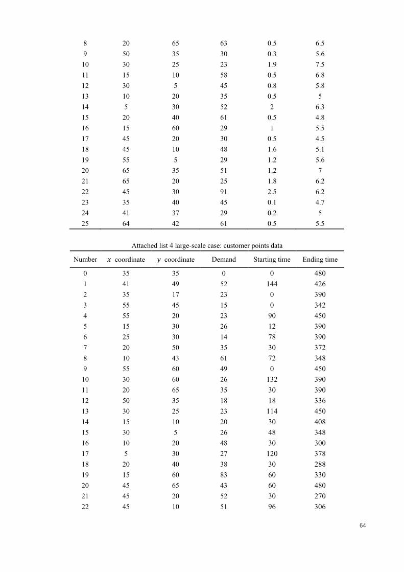
64
8 20 65 63 0.5 6.5 9 50 35 30 0.3 5.6 10 30 25 23 1.9 7.5 11 15 10 58 0.5 6.8 12 30 5 45 0.8 5.8 13 10 20 35 0.5 5 14 5 30 52 2 6.3 15 20 40 61 0.5 4.8 16 15 60 29 1 5.5 17 45 20 30 0.5 4.5 18 45 10 48 1.6 5.1 19 55 5 29 1.2 5.6 20 65 35 51 1.2 7 21 65 20 25 1.8 6.2 22 45 30 91 2.5 6.2 23 35 40 45 0.1 4.7 24 41 37 29 0.2 5 25 64 42 61 0.5 5.5
Attached list 4 large-scale case: customer points data
Number 𝑥 coordinate 𝑦 coordinate Demand Starting time Ending time
0 35 35 0 0 480 1 41 49 52 144 426 2 35 17 23 0 390 3 55 45 15 0 342 4 55 20 23 90 450 5 15 30 26 12 390 6 25 30 14 78 390 7 20 50 35 30 372 8 10 43 61 72 348 9 55 60 49 0 450 10 30 60 26 132 390 11 20 65 35 30 390 12 50 35 18 18 336 13 30 25 23 114 450 14 15 10 20 30 408 15 30 5 26 48 348 16 10 20 48 30 300 17 5 30 27 120 378 18 20 40 38 30 288 19 15 60 83 60 330 20 45 65 43 60 480 21 45 20 52 30 270 22 45 10 51 96 306

65
23 55 5 15 72 336 24 65 35 72 72 420 25 65 20 46 108 372 26 45 30 26 150 372 27 35 40 37 6 282 28 41 37 48 12 300 29 64 42 73 30 330 30 40 60 46 12 414 31 31 52 29 0 390 32 35 69 41 18 468 33 53 52 11 6 408 34 65 55 14 72 402 35 63 65 37 24 480 36 2 60 34 30 432 37 20 20 36 72 474 38 5 5 61 48 390 39 60 12 56 12 456 40 40 25 26 18 414 41 42 7 36 48 480 42 24 12 47 0 390 43 23 3 44 90 444 44 11 14 18 60 390 45 6 38 16 12 456 46 2 48 41 72 468 47 8 56 27 12 450 48 13 52 36 66 414 49 6 68 30 78 402 50 47 47 13 72 480 51 49 58 10 12 336 52 27 43 25 0 414 53 37 31 71 48 432 54 57 29 26 126 468 55 63 23 36 36 480 56 53 12 16 96 474 57 32 12 49 48 408 58 36 26 30 78 480 59 21 24 62 0 456 60 17 34 15 72 468
P-center code
disbak = dis; ite = 0; valite = []; while 1
66
ref = zeros(N,1); k = size(dis,1); ite = ite+1; for i = 1: N coor = client(i,2:3); [val,ind] = min(sum((dis(:,2:3)-repmat(coor,k,1)).^2,2)); ref(i) = ind; end disite = 0; % calculate the total distance for i = 1: N disite = disite + sum((dis(ref(i),2:3)-client(i,2:3)).^2); end valite = [valite,disite]; klist = unique(ref); if length(unique(ref)) ==p break; end if length(unique(ref))>p % drop addval = zeros(length(unique(ref)),1); for i = 1: length(unique(ref)) droppoint = klist(i); clientdrop = find(ref==droppoint); % find other closer location for j = 1: length(clientdrop) coor = client(clientdrop(j),2:3); disleft = dis; disleft (droppoint, :) = []; addval(i) = addval(i) + min(sum((disleft(:,2:3)-repmat(coor,length(disleft(:,2:3)),1)).^2,2)) -
sum((coor-dis(droppoint,2:3)).^2); end end [~, ii] = min(addval); dis (ii, :) = []; end end
Main Program Code
clear all close all

67
%% GENETIC ALGORITHM INITIALIZATION Nite = 150; % iteration number Npop = 100; % population size pcross = 0.9; % crossover probability pmutate = 0.1; % mutation probability % Generating initial population population = zeros (Npop, Nclient+2*Nstation+Kvehecal+1); offspring = zeros (Npop, Nclient+2*Nstation+Kvehecal+1); bestfitness = zeros (Nite, 1); bestpop = zeros (Nite, Nclient+2*Nstation+Kvehecal+1); cnt = 1; while 1 [p1,p2,p3] = popinit; fff = checkroute(p3); if checkroute(p3) population (cnt, :) = p3; cnt = cnt+1; end if cnt > Npop break; end end for ite = 1: Nite fprintf('ite %d\n',ite) fval = zeros(Npop,1); for i = 1: Npop fval(i) = fitness (population(i, :)); end % Selection % Sort the fitness values in descending order, keep the top 2% chromosomes as elite individuals in the new
generation. [fvalnew,Ipos] = sort(fval,'descend'); tournamentSize=2; for k=1: Npop for i=1: tournamentSize randomRow = randi(Npop); tourPopDistances(i) = fval(randomRow); end parent1 = max(tourPopDistances); [parent1X, ~] = find (fval==parent1,1, 'first'); parent1Path = population (parent1X, :);
68
for i=1:tournamentSize randomRow = randi(Npop); tourPopDistances(i) = fval(randomRow); end parent2 = max(tourPopDistances); [parent2X, ~] = find (fval==parent2,1, 'first'); parent2Path = population (parent2X, :); % Crossover % Select the crossover parents, randomly combine all the chromosomes in the population in pairs to form a parent
group, and select one group from it for crossover; parent1Pathcross = parent1Path; if rand(1) <pcross while 1 indcross = randperm(Npop,2); pcross1 = parent1Path; pcross2 = parent2Path; ppc1 = pcross1(1:length(pcross1)-Nstation); ppc2 = pcross2(1:length(pcross2)-Nstation); zeropos1 = find(ppc1==0); ppc1 (zeropos1) = []; zeropos2 = find(ppc2 == 0); ppc2(zeropos2) = []; [pppc1,pppc2] = crossover(ppc1,ppc2); start = 1;p1new = zeros(1,length(ppc1)); for i = 1:length(zeropos1)-1 p1new(zeropos1(i)+1:zeropos1(i+1)-1) = pppc1(start:start+zeropos1(i+1)-zeropos1(i)-2); start = start+zeropos1(i+1)-zeropos1(i)-1; end p1new = [p1new,0]; p1new = [p1new,pcross1(length(pcross1)-Nstation+1:end)]; start = 1;p2new = zeros(1,length(ppc2)); for i = 1:length(zeropos2)-1 p2new(zeropos2(i)+1:zeropos2(i+1)-1) = pppc2(start:start+zeropos2(i+1)-zeropos2(i)-2); start = start+zeropos2(i+1)-zeropos2(i)-1; end p2new = [p2new,0]; p2new = [p2new,pcross2(length(pcross2)-Nstation+1:end)]; if checkroute(p1new) && checkroute(p2new) parent1Pathcross = p1new; break end end end

69
% Mutation if rand(1)<pmutate while 1 indmutate = randi(Npop); pmutate = parent1Pathcross; indzero = find(pmutate(1:length(pmutate)-Nstation)==0); pmutate1 = pmutate(1:length(pmutate)-Nstation); pmutate2 = pmutate(length(pmutate)-Nstation+1:end); p1list = find(pmutate1 > 0 & pmutate1 <= Nclient); mutatepos = randperm(length(p1list),2); temp = p1list(mutatepos(1)); p1list(mutatepos(1)) = p1list(mutatepos(2)); p1list(mutatepos(2)) = temp; if Nstation >1 m2pos = randi(Nstation); if pmutate2(m2pos) == 0 pmutate2(m2pos) = 1; else pmutate2(m2pos) =0; end end pmutate = [pmutate1,pmutate2]; if checkroute(pmutate) parent1Pathcross = pmutate; break; end end end offspring(k,:) = parent1Pathcross; end % Record iteration bestfitness(ite) = fvalnew(1); bestpop(ite,:) = population(Ipos(1),:); population = offspring; end