the logic of relative frustration - soziologie.uni-muenchen.de · problemmodelexperimental...
TRANSCRIPT

Problem Model Experimental design Experimental evidence Discussion References
The Logic of Relative FrustrationBoudon’s Sociological Theory
and Experimental Evidence
Joël Berger Andreas Diekmann
ETH Zürich
Rational Choice Sociology WorkshopVenice International University
November 30, 2011

Problem Model Experimental design Experimental evidence Discussion References
Outline
1 Problem
2 Model
3 Experimental design
4 Experimental evidence
5 Discussion
6 References

Problem Model Experimental design Experimental evidence Discussion References
Puzzling findings: The American Soldier
(Stouffer et al. 1965 [1949])

Problem Model Experimental design Experimental evidence Discussion References
Puzzling findings: The American Soldier
Relative frequency of promoted soldiers (2 years after joining thearmy):
Military Police: 24%, Air Force: 47%

Problem Model Experimental design Experimental evidence Discussion References
Puzzling findings: Tocqueville and the French Revolution
"So it would appear that the Frenchfound their condition the moreunsupportable in proportion to itsimprovement."
(Tocqueville 1856: 214)
Problem Model Experimental design Experimental evidence Discussion References
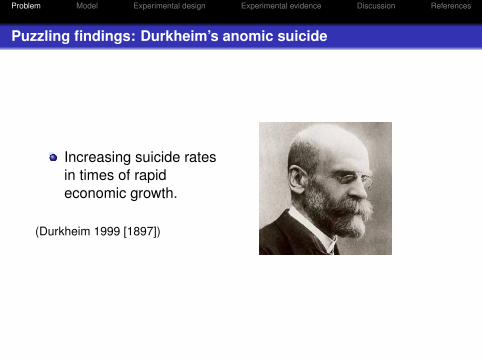
Puzzling findings: Durkheim’s anomic suicide
Increasing suicide ratesin times of rapideconomic growth.
(Durkheim 1999 [1897])

Problem Model Experimental design Experimental evidence Discussion References
Additional chances, more frustration?
Raymond Boudon (1979) presents a game theoretical model,which
... specifies the conditions under which the paradoxicalresult, that additional chances lead to more frustration,occurs.... clarifies the underlying mechanisms.The model has been specified by Raub (1984), expandedby Kosaka (1986) and discussed (e.g. Gambetta 2005).No experimental test.

Problem Model Experimental design Experimental evidence Discussion References
Model set-up
N players face the decision whether or not to investresources C in a competition.
playeri
investC
highpayoff
B – C = d1
loss
d3 – C = d2
notinvestlowpayoff
d3
d1 > d3 > d2

Problem Model Experimental design Experimental evidence Discussion References
Model set-up
number of other investors, (n − 1)0 1 2 ... N−1
player i invest E(0, k) E(1, k) E(2, k) ... E(N−1, k)¬invest d3 d3 d3 ... d3
Einvest(k ,n) =
kn d1 +
n−kn d2 for k < n
d1 for k ≥ n
k : Number of promotion opportunities
n : Number of investors
N : Total number of players

Problem Model Experimental design Experimental evidence Discussion References
Competition and relative frustration
Winners: Actors are satisfied if they invest successfully.Losers: Actors feel relatively frustrated if they invest andlose.Non-investors: Actors not choosing to invest are neutral.Main idea:
When gross benefit B, compared to the costs C and to d3(riskless alternative), is sufficiently high, an increase in kleads to a disproportionate increase in n.As a consequence, there are more additional losers n − kthan additional winners k .

Problem Model Experimental design Experimental evidence Discussion References
Numerical example: k = 1
number of other investors (n − 1)
player i 0 1 2 3 4 5
invest (p) 7.0 2.0 0.3 −0.5 −1.0 −1.3
¬ invest (1− p) 1.0 1.0 1.0 1.0 1.0 1.0
N = 6, k = 1
payoffs: d1 = 7, d2 = −3, d3 = 1
rational solution: mixed strategy with p∗invest = 0.4
E(Inv .) = (1− p)N−1 · E(Inv ., n − 1 = 0) +(N − 1
1
)p(1− p)N−2 · E(Inv ., n − 1 = 1) +(
N − 12
)p2(1− p)N−3 · E(Inv ., n − 1 = 2) +
...+
pN−1 · E(Inv ., n − 1 = N − 1) = d3

Problem Model Experimental design Experimental evidence Discussion References
Model predictions
2020
204040
406060
608080
8010010
0100%
%%1
1
12
2
23
3
34
4
45
5
5k
k
kinvestors
investors
investorslosers
losers
loserswinners
winners
winnersModel predictionsModel predictions
Model predictions

Problem Model Experimental design Experimental evidence Discussion References
Subjects and setting
Subjects: 72 students (ETH Zurich)12 groups of 66 periods432 decisionsCHF 10.– show up feeCHF 12.– for optional investment in the 6 competitions

Problem Model Experimental design Experimental evidence Discussion References
Experimental evidence: satisfaction
00
022
244
466
688
81010
10satisfactionsa
tisfa
ctio
nsatisfactionlow stake
low stake
low stakehigh stake
high stake
high stakelosers
losers
losersnon-investors
non-investors
non-investorswinners
winners
winnerslosers
losers
losersnon-investors
non-investors
non-investorswinners
winners
winners

Problem Model Experimental design Experimental evidence Discussion References
Experimental evidence: investors, losers, winners
00
02020
204040
406060
608080
8010010
0100%
%%1
1
12
2
23
3
34
4
45
5
5k
k
kinvestors (mod)
investors (mod)
investors (mod)losers (mod)
losers (mod)
losers (mod)winners (mod)
winners (mod)
winners (mod)investors (emp)
investors (emp)
investors (emp)losers (emp)
losers (emp)
losers (emp)winners (emp)
winners (emp)
winners (emp)Model predictions and empirical valuesModel predictions and empirical values
Model predictions and empirical values
Problem Model Experimental design Experimental evidence Discussion References
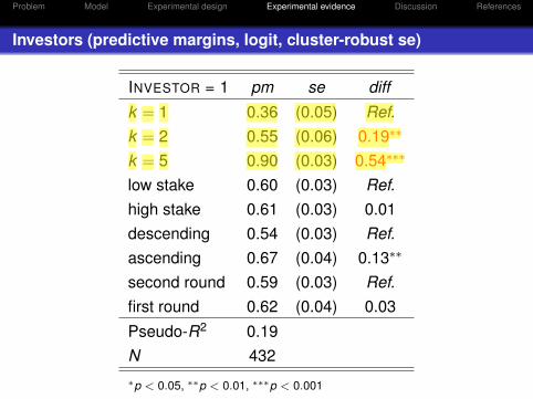
Investors (predictive margins, logit, cluster-robust se)
INVESTOR = 1 pm se diff
k = 1 0.36 (0.05) Ref.k = 2 0.55 (0.06) 0.19∗∗
k = 5 0.90 (0.03) 0.54∗∗∗
low stake 0.60 (0.03) Ref.high stake 0.61 (0.03) 0.01descending 0.54 (0.03) Ref.ascending 0.67 (0.04) 0.13∗∗
second round 0.59 (0.03) Ref.first round 0.62 (0.04) 0.03
Pseudo-R2 0.19N 432∗p < 0.05, ∗∗p < 0.01, ∗∗∗p < 0.001

Problem Model Experimental design Experimental evidence Discussion References
Losers (predictive margins, logit, cluster-robust se)
LOSER = 1 pm se diff
k = 1 0.21 (0.05) Ref.k = 2 0.23 (0.05) 0.02k = 5 0.10 (0.02) −.10∗
low stake 0.19 (0.03) Ref.high stake 0.18 (0.03) −.00descending 0.13 (0.02) Ref.ascending 0.24 (0.03) 0.11∗∗∗
second round 0.17 (0.03) Ref.first round 0.19 (0.03) 0.03
Pseudo-R2 0.05N 432∗p < 0.05, ∗∗p < 0.01, ∗∗∗p < 0.001

Problem Model Experimental design Experimental evidence Discussion References
Satisfaction (predictions, OLS, cluster-robust se)
SATISFACTION y se diff
k = 1 5.2 (0.36) Ref.k = 2 5.5 (0.33) 0.35k = 5 7.5 (0.30) 2.30∗∗∗
low stake 5.7 (0.34) Ref.high stake 6.4 (0.32) 0.74∗∗
descending 6.3 (0.31) Ref.ascending 5.8 (0.35) −0.45second round 6.2 (0.30) Ref.first round 5.9 (0.35) −0.25
R2 0.10N 432∗p < 0.05, ∗∗p < 0.01, ∗∗∗p < 0.001

Problem Model Experimental design Experimental evidence Discussion References
Discussion
Especially when there are 2 promotion chances, playersinvest more cautiously than the model predicts.As a consequence, the rate of frustrated losers remainsconstant.Therefore, the paradoxical effect, that higher opportunitieslead to less mean satisfaction, does not occur.

Problem Model Experimental design Experimental evidence Discussion References
Discussion
satis
fact
ion
k
model prediction intuitionempirical values

Problem Model Experimental design Experimental evidence Discussion References
Further research
Problem: Within-subjects-design→ order effects
Solution: Between-subjects-design
Opportunities kk = 1 k = 2 k = 5
Invest dominant strategy x
x x

Problem Model Experimental design Experimental evidence Discussion References
References
Boudon, R. (1979): Widersprüche sozialen Handelns. Neuwied.
Durkheim, E. (1999): Der Selbstmord. Frankfurt/Main.
Gambetta, D. (2005): Concatenations of Mechanisms. In: Hedström, P.& Swedberg, R. (Eds.): Social Mechanisms. Cambridge.
Kosaka, K. (1986): A Model of Relative Deprivation. Journal ofMathematical Sociology, 12.
Raub, W. (1984): Rationale Akteure, institutionelle Regelungen undInterdependenzen. Frankfurt am Main.
Stouffer, S. et al. (1965): The American Soldier. Manhatten (Kansas).
Tocqueville, A. (1856): The Old Regime and the French Revolution.New York.