the logistic procedure
TRANSCRIPT

Chapter 39The LOGISTIC Procedure
Chapter Table of Contents
OVERVIEW . . . . . . . . . . . . . . . . . . . . . . . . . . . . . . . . . . .1903
GETTING STARTED . . . . . . . . . . . . . . . . . . . . . . . . . . . . . .1906
SYNTAX . . . . . . . . . . . . . . . . . . . . . . . . . . . . . . . . . . . . .1910PROC LOGISTIC Statement . . . . . . . . . . . . . . . . . . . . . . . . . .1910BY Statement . . . . . . . . . . . . . . . . . . . . . . . . . . . . . . . . . .1912CLASS Statement . . . . . . . . . . . . . . . . . . . . . . . . . . . . . . . .1913CONTRAST Statement . .. . . . . . . . . . . . . . . . . . . . . . . . . . .1916FREQ Statement . . . . . . . . . . . . . . . . . . . . . . . . . . . . . . . .1919MODEL Statement . . . . . . . . . . . . . . . . . . . . . . . . . . . . . . .1919OUTPUT Statement . . . . . . . . . . . . . . . . . . . . . . . . . . . . . .1932TEST Statement. . . . . . . . . . . . . . . . . . . . . . . . . . . . . . . . .1937UNITS Statement . . . . . . . . . . . . . . . . . . . . . . . . . . . . . . . .1938WEIGHT Statement . . . . . . . . . . . . . . . . . . . . . . . . . . . . . .1938
DETAILS . . . . . . . . . . . . . . . . . . . . . . . . . . . . . . . . . . . . .1939Missing Values . . . . . . . . . . . . . . . . . . . . . . . . . . . . . . . . .1939Response Level Ordering .. . . . . . . . . . . . . . . . . . . . . . . . . . .1939Link Functions and the Corresponding Distributions . . .. . . . . . . . . . .1940Determining Observations for Likelihood Contributions .. . . . . . . . . . .1941Iterative Algorithms for Model-Fitting. . . . . . . . . . . . . . . . . . . . .1942Convergence Criteria . . .. . . . . . . . . . . . . . . . . . . . . . . . . . .1944Existence of Maximum Likelihood Estimates .. . . . . . . . . . . . . . . .1944Effect Selection Methods .. . . . . . . . . . . . . . . . . . . . . . . . . . .1945Model Fitting Information . . . . . . . . . . . . . . . . . . . . . . . . . . .1947Generalized Coefficient of Determination . . . . . . . . . . . . . . . . . . .1948Score Statistics and Tests . . . . . . . . . . . . . . . . . . . . . . . . . . . .1948Confidence Intervals for Parameters . . . . . . . . . . . . . . . . . . . . . .1950Odds Ratio Estimation . . . . . . . . . . . . . . . . . . . . . . . . . . . . .1952Rank Correlation of Observed Responses and Predicted Probabilities. . . . . 1955Linear Predictor, Predicted Probability, and Confidence Limits . . .. . . . . 1955Classification Table. . . . . . . . . . . . . . . . . . . . . . . . . . . . . . .1956Overdispersion . . . . . . . . . . . . . . . . . . . . . . . . . . . . . . . . .1958The Hosmer-Lemeshow Goodness-of-Fit Test .. . . . . . . . . . . . . . . .1961Receiver Operating Characteristic Curves . . .. . . . . . . . . . . . . . . .1962

1902 � Chapter 39. The LOGISTIC Procedure
Testing Linear Hypotheses about the Regression Coefficients. . . . . . . . .1963Regression Diagnostics . .. . . . . . . . . . . . . . . . . . . . . . . . . . .1963OUTEST= Output Data Set. . . . . . . . . . . . . . . . . . . . . . . . . . .1966INEST= Data Set. . . . . . . . . . . . . . . . . . . . . . . . . . . . . . . .1967OUT= Output Data Set . . . . . . . . . . . . . . . . . . . . . . . . . . . . .1967OUTROC= Data Set . . . . . . . . . . . . . . . . . . . . . . . . . . . . . .1968Computational Resources . . . . . . . . . . . . . . . . . . . . . . . . . . . .1968Displayed Output . . . . . . . . . . . . . . . . . . . . . . . . . . . . . . . .1969ODS Table Names . . . . . . . . . . . . . . . . . . . . . . . . . . . . . . .1972
EXAMPLES . . . . . . . . . . . . . . . . . . . . . . . . . . . . . . . . . . .1974Example 39.1 Stepwise Logistic Regression and Predicted Values .. . . . . 1974Example 39.2 Ordinal Logistic Regression . . .. . . . . . . . . . . . . . . .1988Example 39.3 Logistic Modeling with Categorical Predictors . . . . . . . . .1992Example 39.4 Logistic Regression Diagnostics. . . . . . . . . . . . . . . .1998Example 39.5 Stratified Sampling . . . . . . . . . . . . . . . . . . . . . . .2012Example 39.6 ROC Curve, Customized Odds Ratios, Goodness-of-Fit Statis-
tics, R-Square, and Confidence Limits . . . . . . . . . . . . .2013Example 39.7 Goodness-of-Fit Tests and Subpopulations. . . . . . . . . . .2017Example 39.8 Overdispersion . . . . . . . . . . . . . . . . . . . . . . . . . .2021Example 39.9 Conditional Logistic Regression for Matched Pairs Data. . . . 2026Example 39.10 Complementary Log-Log Model for Infection Rates . . . . .2030Example 39.11 Complementary Log-Log Model for Interval-censored Sur-
vival Times . . . . . . . . . . . . . . . . . . . . . . . . . . .2035
REFERENCES . . . . . . . . . . . . . . . . . . . . . . . . . . . . . . . . . .2040
SAS OnlineDoc: Version 8

Chapter 39The LOGISTIC Procedure
Overview
Binary responses (for example, success and failure) and ordinal responses (for ex-ample, normal, mild, and severe) arise in many fields of study. Logistic regressionanalysis is often used to investigate the relationship between these discrete responsesand a set of explanatory variables. Several texts that discuss logistic regression areCollett (1991), Agresti (1990), Cox and Snell (1989), and Hosmer and Lemeshow(1989).
For binary response models, the response, Y, of an individual or an experimentalunit can take on one of two possible values, denoted for convenience by 1 and 2(for example, Y= 1 if a disease is present, otherwise Y= 2). Supposex is a vectorof explanatory variables andp = Pr(Y = 1 j x) is the response probability to bemodeled. The linear logistic model has the form
logit(p) � log
�p
1� p
�= �+ �0x
where� is the intercept parameter and� is the vector of slope parameters. Notice thatthe LOGISTIC procedure, by default, models the probability of thelower responselevels.
The logistic model shares a common feature with a more general class of linear mod-els, that a functiong = g(�) of the mean of the response variable is assumed to belinearly related to the explanatory variables. Since the mean� implicitly depends onthe stochastic behavior of the response, and the explanatory variables are assumed tobe fixed, the functiong provides the link between the random (stochastic) componentand the systematic (deterministic) component of the response variable Y. For this rea-son, Nelder and Wedderburn (1972) refer tog(�) as a link function. One advantage ofthe logit function over other link functions is that differences on the logistic scale areinterpretable regardless of whether the data are sampled prospectively or retrospec-tively (McCullagh and Nelder 1989, Chapter 4). Other link functions that are widelyused in practice are the probit function and the complementary log-log function. TheLOGISTIC procedure enables you to choose one of these link functions, resulting infitting a broader class of binary response models of the form
g(p) = �+ �0x
For ordinal response models, the response, Y, of an individual or an experimental unitmay be restricted to one of a (usually small) number,k+1(k � 1), of ordinal values,denoted for convenience by1; : : : ; k; k + 1. For example, the severity of coronary

1904 � Chapter 39. The LOGISTIC Procedure
disease can be classified into three response categories as 1=no disease, 2=anginapectoris, and 3=myocardial infarction. The LOGISTIC procedure fits a commonslopes cumulative model, which is a parallel lines regression model based on thecumulative probabilities of the response categories rather than on their individualprobabilities. The cumulative model has the form
g(Pr(Y � i j x)) = �i + �0x; 1 � i � k
where�1; : : : ; �k arek intercept parameters, and� is the vector of slope parame-ters. This model has been considered by many researchers. Aitchison and Silvey(1957) and Ashford (1959) employ a probit scale and provide a maximum likelihoodanalysis; Walker and Duncan (1967) and Cox and Snell (1989) discuss the use of thelog-odds scale. For the log-odds scale, the cumulative logit model is often referred toas theproportional oddsmodel.
The LOGISTIC procedure fits linear logistic regression models for binary or ordinalresponse data by the method of maximum likelihood. The maximum likelihood esti-mation is carried out with either the Fisher-scoring algorithm or the Newton-Raphsonalgorithm. You can specify starting values for the parameter estimates. The logit linkfunction in the logistic regression models can be replaced by the probit function orthe complementary log-log function.
The LOGISTIC procedure provides four variable selection methods: forward selec-tion, backward elimination, stepwise selection, and best subset selection. The bestsubset selection is based on the likelihood score statistic. This method identifies aspecified number of best models containing one, two, three variables and so on, up toa single model containing all the explanatory variables.
Odds ratio estimates are displayed along with parameter estimates. You can also spec-ify the change in the explanatory variables for which odds ratio estimates are desired.Confidence intervals for the regression parameters and odds ratios can be computedbased either on the profile likelihood function or on the asymptotic normality of theparameter estimators.
Various methods to correct for overdispersion are provided, including Williams’method for grouped binary response data. The adequacy of the fitted model can beevaluated by various goodness-of-fit tests, including the Hosmer-Lemeshow test forbinary response data.
The LOGISTIC procedure enables you to specify categorical variables (also known asCLASS variables) as explanatory variables. It also enables you to specify interactionterms in the same way as in the GLM procedure.
The LOGISTIC procedure allows either a full-rank parameterization or a less thanfull-rank parameterization. The full-rank parameterization offers four coding meth-ods: effect, reference, polynomial, and orthogonal polynomial. The effect coding isthe same method that is used in the CATMOD procedure. The less than full-rankparameterization is the same coding as that used in the GLM and GENMOD proce-dures.
SAS OnlineDoc: Version 8

Overview � 1905
The LOGISTIC procedure has some additional options to control how to move effects(either variables or interactions) in and out of a model with various model-buildingstrategies such as forward selection, backward elimination, or stepwise selection.When there are no interaction terms, a main effect can enter or leave a model in asingle step based on thep-value of the score or Wald statistic. When there are in-teraction terms, the selection process also depends on whether you want to preservemodel hierarchy. These additional options enable you to specify whether model hier-archy is to be preserved, how model hierarchy is applied, and whether a single effector multiple effects can be moved in a single step.
Like many procedures in SAS/STAT software that allow the specification of CLASSvariables, the LOGISTIC procedure provides a CONTRAST statement for specify-ing customized hypothesis tests concerning the model parameters. The CONTRASTstatement also provides estimation of individual rows of contrasts, which is particu-larly useful for obtaining odds ratio estimates for various levels of the CLASS vari-ables.
Further features of the LOGISTIC procedure enable you to
� control the ordering of the response levels
� compute a generalizedR2 measure for the fitted model
� reclassify binary response observations according to their predicted responseprobabilities
� test linear hypotheses about the regression parameters
� create a data set for producing a receiver operating characteristic curve for eachfitted model
� create a data set containing the estimated response probabilities, residuals, andinfluence diagnostics
The remaining sections of this chapter describe how to use PROC LOGISTIC anddiscuss the underlying statistical methodology. The “Getting Started” section in-troduces PROC LOGISTIC with an example for binary response data. The “Syntax”section (page 1910) describes the syntax of the procedure. The “Details” section(page 1939) summarizes the statistical technique employed by PROC LOGISTIC.The “Examples” section (page 1974) illustrates the use of the LOGISTIC procedurewith 10 applications.
For more examples and discussion on the use of PROC LOGISTIC, refer to Stokes,Davis, and Koch (1995) and toLogistic Regression Examples Using the SAS System.
SAS OnlineDoc: Version 8

1906 � Chapter 39. The LOGISTIC Procedure
Getting Started
The LOGISTIC procedure is similar in use to the other regression procedures in theSAS System. To demonstrate the similarity, suppose the response variabley is binaryor ordinal, andx1 andx2 are two explanatory variables of interest. To fit a logisticregression model, you can use a MODEL statement similar to that used in the REGprocedure:
proc logistic;model y=x1 x2;
run;
The response variabley can be either character or numeric. PROC LOGISTIC enu-merates the total number of response categories and orders the response levels ac-cording to the ORDER= option in the PROC LOGISTIC statement. The procedurealso allows the input of binary response data that are grouped:
proc logistic;model r/n=x1 x2;
run;
Here,n represents the number of trials andr represents the number of events.
The following example illustrates the use of PROC LOGISTIC. The data, taken fromCox and Snell (1989, pp. 10–11), consist of the number,r, of ingots not ready forrolling, out of n tested, for a number of combinations of heating time and soakingtime. The following invocation of PROC LOGISTIC fits the binary logit model tothe grouped data:
data ingots;input Heat Soak r n @@;datalines;
7 1.0 0 10 14 1.0 0 31 27 1.0 1 56 51 1.0 3 137 1.7 0 17 14 1.7 0 43 27 1.7 4 44 51 1.7 0 17 2.2 0 7 14 2.2 2 33 27 2.2 0 21 51 2.2 0 17 2.8 0 12 14 2.8 0 31 27 2.8 1 22 51 4.0 0 17 4.0 0 9 14 4.0 0 19 27 4.0 1 16;
proc logistic data=ingots;model r/n=Heat Soak;
run;
The results of this analysis are shown in the following tables.
SAS OnlineDoc: Version 8

Getting Started � 1907
The SAS System
The LOGISTIC Procedure
Model Information
Data Set WORK.INGOTSResponse Variable (Events) rResponse Variable (Trials) nNumber of Observations 19Link Function LogitOptimization Technique Fisher’s scoring
PROC LOGISTIC first lists background information about the fitting of the model.Included are the name of the input data set, the response variable(s) used, the numberof observations used, and the link function used.
The LOGISTIC Procedure
Response Profile
Ordered Binary TotalValue Outcome Frequency
1 Event 122 Nonevent 375
Model Convergence Status
Convergence criterion (GCONV=1E-8) satisfied.
The “Response Profile” table lists the response categories (which are EVENT andNO EVENT when grouped data are input), their ordered values, and their total fre-quencies for the given data.
The LOGISTIC Procedure
Model Fit Statistics
InterceptIntercept and
Criterion Only Covariates
AIC 108.988 101.346SC 112.947 113.221-2 Log L 106.988 95.346
Testing Global Null Hypothesis: BETA=0
Test Chi-Square DF Pr > ChiSq
Likelihood Ratio 11.6428 2 0.0030Score 15.1091 2 0.0005Wald 13.0315 2 0.0015
SAS OnlineDoc: Version 8

1908 � Chapter 39. The LOGISTIC Procedure
The “Model Fit Statistics” table contains the Akaike Information Criterion (AIC),the Schwarz Criterion (SC), and the negative of twice the log likelihood (-2 LogL) for the intercept-only model and the fitted model. AIC and SC can be used tocompare different models, and the ones with smaller values are preferred. Results ofthe likelihood ratio test and the efficient score test for testing the joint significance ofthe explanatory variables (Soak andHeat) are included in the “Testing Global NullHypothesis: BETA=0” table.
The LOGISTIC Procedure
Analysis of Maximum Likelihood Estimates
StandardParameter DF Estimate Error Chi-Square Pr > ChiSq
Intercept 1 -5.5592 1.1197 24.6503 <.0001Heat 1 0.0820 0.0237 11.9454 0.0005Soak 1 0.0568 0.3312 0.0294 0.8639
Odds Ratio Estimates
Point 95% WaldEffect Estimate Confidence Limits
Heat 1.085 1.036 1.137Soak 1.058 0.553 2.026
The “Analysis of Maximum Likelihood Estimates” table lists the parameter estimates,their standard errors, and the results of the Wald test for individual parameters. Theodds ratio for each slope parameter, estimated by exponentiating the correspondingparameter estimate, is shown in the “Odds Ratios Estimates” table, along with 95%Wald confidence intervals.
Using the parameter estimates, you can calculate the estimated logit ofp as
�5:5592 + 0:082 � Heat+ 0:0568 � Soak
If Heat=7 andSoak=1, then logit(p) = �4:9284. Using this logit estimate, youcan calculatep as follows:
p = 1=(1 + e4:9284) = 0:0072
This gives the predicted probability of the event (ingot not ready for rolling) forHeat=7 andSoak=1. Note that PROC LOGISTIC can calculate these statisticsfor you; use the OUTPUT statement with the P= option.
SAS OnlineDoc: Version 8

Getting Started � 1909
The LOGISTIC Procedure
Association of Predicted Probabilities and Observed Responses
Percent Concordant 64.4 Somers’ D 0.460Percent Discordant 18.4 Gamma 0.555Percent Tied 17.2 Tau-a 0.028Pairs 4500 c 0.730
Finally, the “Association of Predicted Probabilities and Observed Responses” tablecontains four measures of association for assessing the predictive ability of a model.They are based on the number of pairs of observations with different response val-ues, the number of concordant pairs, and the number of discordant pairs, which arealso displayed. Formulas for these statistics are given in the “Rank Correlation ofObserved Responses and Predicted Probabilities” section on page 1955.
To illustrate the use of an alternative form of input data, the following program cre-ates the INGOTS data set with new variablesNotReady andFreq instead ofn andr. The variableNotReady represents the response of individual units; it has a valueof 1 for units not ready for rolling (event) and a value of 0 for units ready for rolling(nonevent). The variableFreq represents the frequency of occurrence of each com-bination ofHeat, Soak, andNotReady. Note that, compared to the previous dataset,NotReady=1 impliesFreq=r, andNotReady=0 impliesFreq=n�r.
data ingots;input Heat Soak NotReady Freq @@;datalines;
7 1.0 0 10 14 1.0 0 31 14 4.0 0 19 27 2.2 0 21 51 1.0 1 37 1.7 0 17 14 1.7 0 43 27 1.0 1 1 27 2.8 1 1 51 1.0 0 107 2.2 0 7 14 2.2 1 2 27 1.0 0 55 27 2.8 0 21 51 1.7 0 17 2.8 0 12 14 2.2 0 31 27 1.7 1 4 27 4.0 1 1 51 2.2 0 17 4.0 0 9 14 2.8 0 31 27 1.7 0 40 27 4.0 0 15 51 4.0 0 1;
The following SAS statements invoke PROC LOGISTIC to fit the same model usingthe alternative form of the input data set.
proc logistic data=ingots descending;model NotReady = Soak Heat;freq Freq;
run;
Results of this analysis are the same as the previous one. The displayed output forthe two runs are identical except for the background information of the model fit andthe “Response Profile” table.
PROC LOGISTIC models the probability of the response level that corresponds to theOrdered Value 1 as displayed in the “Response Profile” table. By default, OrderedValues are assigned to the sorted response values in ascending order.
SAS OnlineDoc: Version 8

1910 � Chapter 39. The LOGISTIC Procedure
The DESCENDING option reverses the default ordering of the response values sothatNotReady=1 corresponds to the Ordered Value 1 andNotReady=0 correspondsto the Ordered Value 2, as shown in the following table:
The LOGISTIC Procedure
Response Profile
Ordered TotalValue NotReady Frequency
1 1 122 0 375
If the ORDER= option and the DESCENDING option are specified together, the re-sponse levels are ordered according to the ORDER= option and then reversed. Youshould always check the “Response Profile” table to ensure that the outcome of inter-est has been assigned Ordered Value 1. See the “Response Level Ordering” sectionon page 1939 for more detail.
Syntax
The following statements are available in PROC LOGISTIC:
PROC LOGISTIC < options >;BY variables ;CLASS variable <(v-options)> <variable <(v-options)>... >
< / v-options >;CONTRAST ’label’ effect values <,... effect values>< =options >;FREQ variable ;MODEL response = < effects >< / options >;MODEL events/trials = < effects >< / options >;OUTPUT < OUT=SAS-data-set >
< keyword=name: : :keyword=name > / < option >;< label: > TEST equation1 < , : : : , < equationk >>< /option >;UNITS independent1 = list1 < : : : independentk = listk >< /option > ;WEIGHT variable </ option >;
The PROC LOGISTIC and MODEL statements are required; only one MODEL state-ment can be specified. The CLASS statement (if used) must precede the MODELstatement, and the CONTRAST statement (if used) must follow the MODEL state-ment. The rest of this section provides detailed syntax information for each of thepreceding statements, beginning with the PROC LOGISTIC statement. The remain-ing statements are covered in alphabetical order.
SAS OnlineDoc: Version 8

PROC LOGISTIC Statement � 1911
PROC LOGISTIC Statement
PROC LOGISTIC < options >;
The PROC LOGISTIC statement starts the LOGISTIC procedure and optionallyidentifies input and output data sets, controls the ordering of the response levels,and suppresses the display of results.
COVOUTadds the estimated covariance matrix to the OUTEST= data set. For the COVOUToption to have an effect, the OUTEST= option must be specified. See the section“OUTEST= Output Data Set” on page 1966 for more information.
DATA=SAS-data-setnames the SAS data set containing the data to be analyzed. If you omit the DATA=option, the procedure uses the most recently created SAS data set.
DESCENDINGDESC
reverses the sorting order for the levels of the response variable. If both theDESCENDING and ORDER= options are specified, PROC LOGISTIC orders thelevels according to the ORDER= option and then reverses that order. See the “Re-sponse Level Ordering” section on page 1939 for more detail.
INEST= SAS-data-setnames the SAS data set that contains initial estimates for all the parameters in themodel. BY-group processing is allowed in setting up the INEST= data set. See thesection “INEST= Data Set” on page 1967 for more information.
NAMELEN=nspecifies the length of effect names in tables and output data sets to ben characters,wheren is a value between 20 and 200. The default length is 20 characters.
NOPRINTsuppresses all displayed output. Note that this option temporarily disables the OutputDelivery System (ODS); see Chapter 15, “Using the Output Delivery System,” formore information.
ORDER=DATA | FORMATTED | FREQ | INTERNALRORDER=DATA | FORMATTED | INTERNAL
specifies the sorting order for the levels of the response variable. When OR-DER=FORMATTED (the default) for numeric variables for which you have suppliedno explicit format (that is, for which there is no corresponding FORMAT statementin the current PROC LOGISTIC run or in the DATA step that created the data set),the levels are ordered by their internal (numeric) value. Note that this represents achange from previous releases for how class levels are ordered. In releases previ-ous to Version 8, numeric class levels with no explicit format were ordered by theirBEST12. formatted values, and in order to revert to the previous ordering you canspecify this format explicitly for the affected classification variables. The changewas implemented because the former default behavior for ORDER=FORMATTED
SAS OnlineDoc: Version 8

1912 � Chapter 39. The LOGISTIC Procedure
often resulted in levels not being ordered numerically and usually required the userto intervene with an explicit format or ORDER=INTERNAL to get the more naturalordering. The following table shows how PROC LOGISTIC interprets values of theORDER= option.
Value of ORDER= Levels Sorted ByDATA order of appearance in the input data set
FORMATTED external formatted value, except for numericvariables with no explicit format, which aresorted by their unformatted (internal) value
FREQ descending frequency count; levels with themost observations come first in the order
INTERNAL unformatted value
By default, ORDER=FORMATTED. For FORMATTED and INTERNAL, the sortorder is machine dependent. For more information on sorting order, see the chapteron the SORT procedure in theSAS Procedures Guideand the discussion of BY-groupprocessing inSAS Language Reference: Concepts.
OUTEST= SAS-data-setcreates an output SAS data set that contains the final parameter estimates and, option-ally, their estimated covariances (see the preceding COVOUT option). The names ofthe variables in this data set are the same as those of the explanatory variables in theMODEL statement plus the nameIntercept for the intercept parameter in the caseof a binary response model. For an ordinal response model with more than two re-sponse categories, the parameters are named Intercept, Intercept2, Intercept3, and soon. The output data set also includes a variable named–LNLIKE– , which containsthe log likelihood.
See the section “OUTEST= Output Data Set” on page 1966 for more information.
SIMPLEdisplays simple descriptive statistics (mean, standard deviation, minimum and maxi-mum) for each explanatory variable in the MODEL statement. The SIMPLE optiongenerates a breakdown of the simple descriptive statistics for the entire data set andalso for individual response levels. The NOSIMPLE option suppresses this outputand is the default.
BY Statement
BY variables ;
You can specify a BY statement with PROC LOGISTIC to obtain separate analy-ses on observations in groups defined by the BY variables. When a BY statementappears, the procedure expects the input data set to be sorted in order of the BYvariables. Thevariablesare one or more variables in the input data set.
SAS OnlineDoc: Version 8

CLASS Statement � 1913
If your input data set is not sorted in ascending order, use one of the following alter-natives:
� Sort the data using the SORT procedure with a similar BY statement.
� Specify the BY statement option NOTSORTED or DESCENDING in the BYstatement for the LOGISTIC procedure. The NOTSORTED option does notmean that the data are unsorted but rather that the data are arranged in groups(according to values of the BY variables) and that these groups are not neces-sarily in alphabetical or increasing numeric order.
� Create an index on the BY variables using the DATASETS procedure (in baseSAS software).
For more information on the BY statement, refer to the discussion inSAS LanguageReference: Concepts. For more information on the DATASETS procedure, refer tothe discussion in theSAS Procedures Guide.
CLASS Statement
CLASS variable <(v-options)> <variable <(v-options)>... >< / v-options >;
The CLASS statement names the classification variables to be used in the analysis.The CLASS statement must precede the MODEL statement. You can specify vari-ousv-optionsfor each variable by enclosing them in parentheses after the variablename. You can also specify globalv-optionsfor the CLASS statement by placingthem after a slash (/). Globalv-optionsare applied to all the variables specified inthe CLASS statement. However, individual CLASS variablev-optionsoverride theglobalv-options.
CPREFIX= nspecifies that, at most, the firstn characters of a CLASS variable name be usedin creating names for the corresponding dummy variables. The default is32 �min(32;max(2; f)), wheref is the formatted length of the CLASS variable.
DESCENDINGDESC
reverses the sorting order of the classification variable.
LPREFIX= nspecifies that, at most, the firstn characters of a CLASS variable label be used increating labels for the corresponding dummy variables.
ORDER=DATA | FORMATTED | FREQ | INTERNALspecifies the sorting order for the levels of classification variables. This ordering de-termines which parameters in the model correspond to each level in the data, so theORDER= option may be useful when you use the CONTRAST statement. When OR-DER=FORMATTED (the default) for numeric variables for which you have suppliedno explicit format (that is, for which there is no corresponding FORMAT statement
SAS OnlineDoc: Version 8

1914 � Chapter 39. The LOGISTIC Procedure
in the current PROC LOGISTIC run or in the DATA step that created the data set),the levels are ordered by their internal (numeric) value. Note that this represents achange from previous releases for how class levels are ordered. In releases previ-ous to Version 8, numeric class levels with no explicit format were ordered by theirBEST12. formatted values, and in order to revert to the previous ordering you canspecify this format explicitly for the affected classification variables. The changewas implemented because the former default behavior for ORDER=FORMATTEDoften resulted in levels not being ordered numerically and usually required the userto intervene with an explicit format or ORDER=INTERNAL to get the more naturalordering. The following table shows how PROC LOGISTIC interprets values of theORDER= option.
Value of ORDER= Levels Sorted ByDATA order of appearance in the input data set
FORMATTED external formatted value, except for numericvariables with no explicit format, which aresorted by their unformatted (internal) value
FREQ descending frequency count; levels with themost observations come first in the order
INTERNAL unformatted value
By default, ORDER=FORMATTED. For FORMATTED and INTERNAL, the sortorder is machine dependent. For more information on sorting order, see the chapteron the SORT procedure in theSAS Procedures Guideand the discussion of BY-groupprocessing inSAS Language Reference: Concepts.
PARAM=keywordspecifies the parameterization method for the classification variable or variables. De-sign matrix columns are created from CLASS variables according to the follow-ing coding schemes. The default is PARAM=EFFECT. If PARAM=ORTHPOLY orPARAM=POLY, and the CLASS levels are numeric, then the ORDER= option in theCLASS statement is ignored, and the internal, unformatted values are used.
EFFECT specifies effect coding
GLM specifies less than full rank, reference cell coding; thisoption can only be used as a global option
ORTHPOLY specifies orthogonal polynomial coding
POLYNOMIAL | POLY specifies polynomial coding
REFERENCE | REF specifies reference cell coding
The EFFECT, POLYNOMIAL, REFERENCE, and ORTHPOLY parameterizationsare full rank. For the EFFECT and REFERENCE parameterizations, the REF= optionin the CLASS statement determines the reference level.
Consider a model with one CLASS variable A with four levels, 1, 2, 5, and 7. Detailsof the possible choices for the PARAM= option follow.
SAS OnlineDoc: Version 8
CLASS Statement � 1915
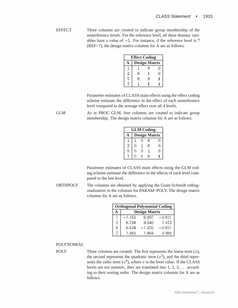
EFFECT Three columns are created to indicate group membership of thenonreference levels. For the reference level, all three dummy vari-ables have a value of�1. For instance, if the reference level is 7(REF=7), the design matrix columns for A are as follows.
Effect CodingA Design Matrix1 1 0 02 0 1 05 0 0 17 �1 �1 �1
Parameter estimates of CLASS main effects using the effect codingscheme estimate the difference in the effect of each nonreferencelevel compared to the average effect over all 4 levels.
GLM As in PROC GLM, four columns are created to indicate groupmembership. The design matrix columns for A are as follows.
GLM CodingA Design Matrix1 1 0 0 02 0 1 0 05 0 0 1 07 0 0 0 1
Parameter estimates of CLASS main effects using the GLM cod-ing scheme estimate the difference in the effects of each level com-pared to the last level.
ORTHPOLY The columns are obtained by applying the Gram-Schmidt orthog-onalization to the columns for PARAM=POLY. The design matrixcolumns for A are as follows.
Orthogonal Polynomial CodingA Design Matrix1 �1:153 0:907 �0:9212 �0:734 �0:540 1:4735 0:524 �1:370 �0:9217 1:363 1:004 0:368
POLYNOMIAL
POLY Three columns are created. The first represents the linear term (x),the second represents the quadratic term (x2), and the third repre-sents the cubic term (x3), wherex is the level value. If the CLASSlevels are not numeric, they are translated into 1, 2, 3,: : : accord-ing to their sorting order. The design matrix columns for A are asfollows.
SAS OnlineDoc: Version 8

1916 � Chapter 39. The LOGISTIC Procedure
Polynomial CodingA Design Matrix1 1 1 12 2 4 85 5 25 1257 7 49 343
REFERENCE
REF Three columns are created to indicate group membership of thenonreference levels. For the reference level, all three dummy vari-ables have a value of 0. For instance, if the reference level is 7(REF=7), the design matrix columns for A are as follows.
Reference CodingA Design Matrix1 1 0 02 0 1 05 0 0 17 0 0 0
Parameter estimates of CLASS main effects using the referencecoding scheme estimate the difference in the effect of each nonref-erence level compared to the effect of the reference level.
REF=’level’ | keywordspecifies the reference level for PARAM=EFFECT or PARAM=REFERENCE. Foran individual (but not a global) variable REF=option, you can specify thelevel ofthe variable to use as the reference level. For a global or individual variable REF=option, you can use one of the followingkeywords. The default is REF=LAST.
FIRST designates the first ordered level as reference
LAST designates the last ordered level as reference
CONTRAST Statement
CONTRAST ’label’ row-description <,... row-description>< =options >;where arow-description is: effect values <,...effect values>
The CONTRAST statement provides a mechanism for obtaining customized hypoth-esis tests. It is similar to the CONTRAST statement in PROC GLM and PROCCATMOD, depending on the coding schemes used with any classification variablesinvolved.
The CONTRAST statement enables you to specify a matrix,L, for testing the hypoth-esisL� = 0. You must be familiar with the details of the model parameterization thatPROC LOGISTIC uses (for more information, see the PARAM= option in the section
SAS OnlineDoc: Version 8

CONTRAST Statement � 1917
“CLASS Statement” on page 1913). Optionally, the CONTRAST statement enablesyou to estimate each row,l0i�, of L� and test the hypothesisl0i� = 0. Computedstatistics are based on the asymptotic chi-square distribution of the Wald statistic.
There is no limit to the number of CONTRAST statements that you can specify, butthey must appear after the MODEL statement.
The following parameters are specified in the CONTRAST statement:
label identifies the contrast on the output. A label is required for every contrastspecified, and it must be enclosed in quotes. Labels can contain up to 256characters.
effect identifies an effect that appears in the MODEL statement. The nameINTERCEPT can be used as an effect when one or more intercepts are in-cluded in the model. You do not need to include all effects that are includedin the MODEL statement.
values are constants that are elements of theL matrix associated with the effect.To correctly specify your contrast, it is crucial to know the ordering ofparameters within each effect and the variable levels associated with anyparameter. The “Class Level Information” table shows the ordering of lev-els within variables. The E option, described later in this section, enablesyou to verify the proper correspondence ofvaluesto parameters.
The rows ofL are specified in order and are separated by commas. Multiple degree-of-freedom hypotheses can be tested by specifying multiplerow-descriptions. Forany of the full-rank parameterizations, if an effect is not specified in the CONTRASTstatement, all of its coefficients in theL matrix are set to 0. If too many values arespecified for an effect, the extra ones are ignored. If too few values are specified, theremaining ones are set to 0.
When you use effect coding (by default or by specifying PARAM=EFFECT in theCLASS statement), all parameters are directly estimable (involve no other param-eters). For example, suppose an effect coded CLASS variableA has four levels.Then there are three parameters (�1; �2; �3) representing the first three levels, andthe fourth parameter is represented by
��1 � �2 � �3
To test the first versus the fourth level ofA, you would test
�1 = ��1 � �2 � �3
or, equivalently,
2�1 + �2 + �3 = 0
SAS OnlineDoc: Version 8

1918 � Chapter 39. The LOGISTIC Procedure
which, in the formL� = 0, is
�2 1 1
� 24 �1�2�3
35 = 0
Therefore, you would use the following CONTRAST statement:
contrast ’1 vs. 4’ A 2 1 1;
To contrast the third level with the average of the first two levels, you would test
�1 + �22
= �3
or, equivalently,
�1 + �2 � 2�3 = 0
Therefore, you would use the following CONTRAST statement:
contrast ’1&2 vs. 3’ A 1 1 -2;
Other CONTRAST statements are constructed similarly. For example,
contrast ’1 vs. 2 ’ A 1 -1 0;contrast ’1&2 vs. 4 ’ A 3 3 2;contrast ’1&2 vs. 3&4’ A 2 2 0;contrast ’Main Effect’ A 1 0 0,
A 0 1 0,A 0 0 1;
When you use the less than full-rank parameterization (by specifying PARAM=GLMin the CLASS statement), each row is checked for estimability. If PROC LOGISTICfinds a contrast to be nonestimable, it displays missing values in corresponding rowsin the results. PROC LOGISTIC handles missing level combinations of classificationvariables in the same manner as PROC GLM. Parameters corresponding to missinglevel combinations are not included in the model. This convention can affect the wayin which you specify theLmatrix in your CONTRAST statement. If the elements ofL are not specified for an effect that contains a specified effect, then the elements ofthe specified effect are distributed over the levels of the higher-order effect just as theGLM procedure does for its CONTRAST and ESTIMATE statements. For example,suppose that the model contains effects A and B and their interaction A*B. If youspecify a CONTRAST statement involving A alone, theL matrix contains nonzeroterms for both A and A*B, since A*B contains A.
The degrees of freedom is the number of linearly independent constraints implied bythe CONTRAST statement, that is, the rank ofL.
SAS OnlineDoc: Version 8

MODEL Statement � 1919
You can specify the following options after a slash (/).
ALPHA= valuespecifies the significance level of the confidence interval for each contrast when theESTIMATE option is specified. The default is ALPHA=.05, resulting in a 95% con-fidence interval for each contrast.
Erequests that theLmatrix be displayed.
ESTIMATE=keywordrequests that each individual contrast (that is, each row,l0i�, of L�) or exponentiated
contrast (el0i�) be estimated and tested. PROC LOGISTIC displays the point esti-
mate, its standard error, a Wald confidence interval and a Wald chi-square test foreach contrast. The significance level of the confidence interval is controlled by theALPHA= option. You can estimate the contrast or the exponentiated contrast (el
0i�),
or both, by specifying one of the followingkeywords:
PARM specifies that the contrast itself be estimated
EXP specifies that the exponentiated contrast be estimated
BOTH specifies that both the contrast and the exponentiated contrast beestimated
SINGULAR = numbertunes the estimability check. This option is ignored when the full-rank parameteriza-tion is used. Ifv is a vector, define ABS(v) to be the absolute value of the elementof v with the largest absolute value. Define C to be equal to ABS(K0) if ABS(K0) isgreater than 0; otherwise, C equals 1 for a rowK0 in the contrast. If ABS(K0 �K0T)is greater than C�number, thenK is declared nonestimable. TheTmatrix is the Her-mite form matrix(X0X)�(X0X), and(X0X)� represents a generalized inverse ofthe matrixX0X. The value fornumber must be between 0 and 1; the default valueis 1E�4.
FREQ Statement
FREQ variable ;
Thevariable in the FREQ statement identifies a variable that contains the frequencyof occurrence of each observation. PROC LOGISTIC treats each observation as if itappearsn times, wheren is the value of the FREQ variable for the observation. If itis not an integer, the frequency value is truncated to an integer. If the frequency valueis less than 1 or missing, the observation is not used in the model fitting. When theFREQ statement is not specified, each observation is assigned a frequency of 1.
SAS OnlineDoc: Version 8

1920 � Chapter 39. The LOGISTIC Procedure
MODEL Statement
MODEL variable= < effects >< /options >;MODEL events/trials= < effects >< / options >;
The MODEL statement names the response variable and the explanatory effects, in-cluding covariates, main effects, interactions, and nested effects. If you omit theexplanatory variables, the procedure fits an intercept-only model.
Two forms of the MODEL statement can be specified. The first form, referred to assingle-trial syntax, is applicable to both binary response data and ordinal responsedata. The second form, referred to asevents/trialssyntax, is restricted to the caseof binary response data. Thesingle-trial syntax is used when each observation inthe DATA= data set contains information on only a single trial, for instance, a singlesubject in an experiment. When each observation contains information on multiplebinary-response trials, such as the counts of the number of subjects observed and thenumber responding, thenevents/trialssyntax can be used.
In thesingle-trial syntax, you specify one variable (preceding the equal sign) as theresponse variable. This variable can be character or numeric. Values of this variableare sorted by the ORDER= option (and the DESCENDING option, if specified) inthe PROC LOGISTIC statement.
In the events/trialssyntax, you specify two variables that contain count data for abinomial experiment. These two variables are separated by a slash. The value ofthe first variable,events, is the number of positive responses (or events). The valueof the second variable,trials, is the number of trials. The values of botheventsand(trials�events) must be nonnegative and the value oftrials must be positive for theresponse to be valid.
For both forms of the MODEL statement, explanatoryeffectsfollow the equal sign.The variables can be either continuous or classification variables. Classification vari-ables can be character or numeric, and they must be declared in the CLASS state-ment. When an effect is a classification variable, the procedure enters a set of codedcolumns into the design matrix instead of directly entering a single column contain-ing the values of the variable. See the section “Specification of Effects” on page 1517of Chapter 30, “The GLM Procedure.”
Table 39.1 summarizes the options available in the MODEL statement.
Table 39.1. Model Statement Options
Option DescriptionModel Specification OptionsLINK= specifies link functionNOINT suppresses interceptNOFIT suppresses model fittingOFFSET= specifies offset variable
SAS OnlineDoc: Version 8

MODEL Statement � 1921
Table 39.1. (continued)
Option DescriptionSELECTION= specifies variable selection method
Variable Selection OptionsBEST= controls the number of models displayed for SCORE selectionDETAILS requests detailed results at each stepFAST uses fast elimination methodHIERARCHY= specifies whether and how hierarchy is maintained and whether a single
effect or multiple effects are allowed to enter or leave the model per stepINCLUDE= specifies number of variables included in every modelMAXSTEP= specifies maximum number of steps for STEPWISE selectionSEQUENTIAL adds or deletes variables in sequential orderSLENTRY= specifies significance level for entering variablesSLSTAY= specifies significance level for removing variablesSTART= specifies the number of variables in first modelSTOP= specifies the number of variables in final modelSTOPRES adds or deletes variables by residual chi-square criterion
Model-Fitting Specification OptionsABSFCONV= specifies the absolute function convergence criterionFCONV= specifies the relative function convergence criterionGCONV= specifies the relative gradient convergence criterionXCONV= specifies the relative parameter convergence criterionMAXITER= specifies maximum number of iterationsNOCHECK suppresses checking for infinite parametersRIDGING= specifies the technique used to improve the log-likelihood function when
its value is worse than that of the previous stepSINGULAR= specifies tolerance for testing singularityTECHNIQUE= specifies iterative algorithm for maximization
Options for Confidence IntervalsALPHA= specifies� for the100(1 � �)% confidence intervalsCLPARM= computes confidence intervals for parametersCLODDS= computes confidence intervals for odds ratiosPLCONV= specifies profile likelihood convergence criterion
Options for Classifying ObservationsCTABLE displays classification tablePEVENT= specifies prior event probabilitiesPPROB= specifies probability cutpoints for classification
Options for Overdispersion and Goodness-of-Fit TestsAGGREGATE= determines subpopulations for Pearson chi-square and devianceSCALE= specifies method to correct overdispersionLACKFIT requests Hosmer and Lemeshow goodness-of-fit test
Options for ROC CurvesOUTROC= names the output data setROCEPS= specifies probability grouping criterion
Options for Regression Diagnostics
SAS OnlineDoc: Version 8
1922 � Chapter 39. The LOGISTIC Procedure
Table 39.1. (continued)
Option DescriptionINFLUENCE displays influence statisticsIPLOTS requests index plots
Options for Display of DetailsCORRB displays correlation matrixCOVB displays covariance matrixEXPB displays the exponentiated values of estimatesITPRINT displays iteration historyNODUMMYPRINT suppresses the “Class Level Information” tablePARMLABEL displays the parameter labelsRSQUARE displays generalizedR2
STB displays the standardized estimates
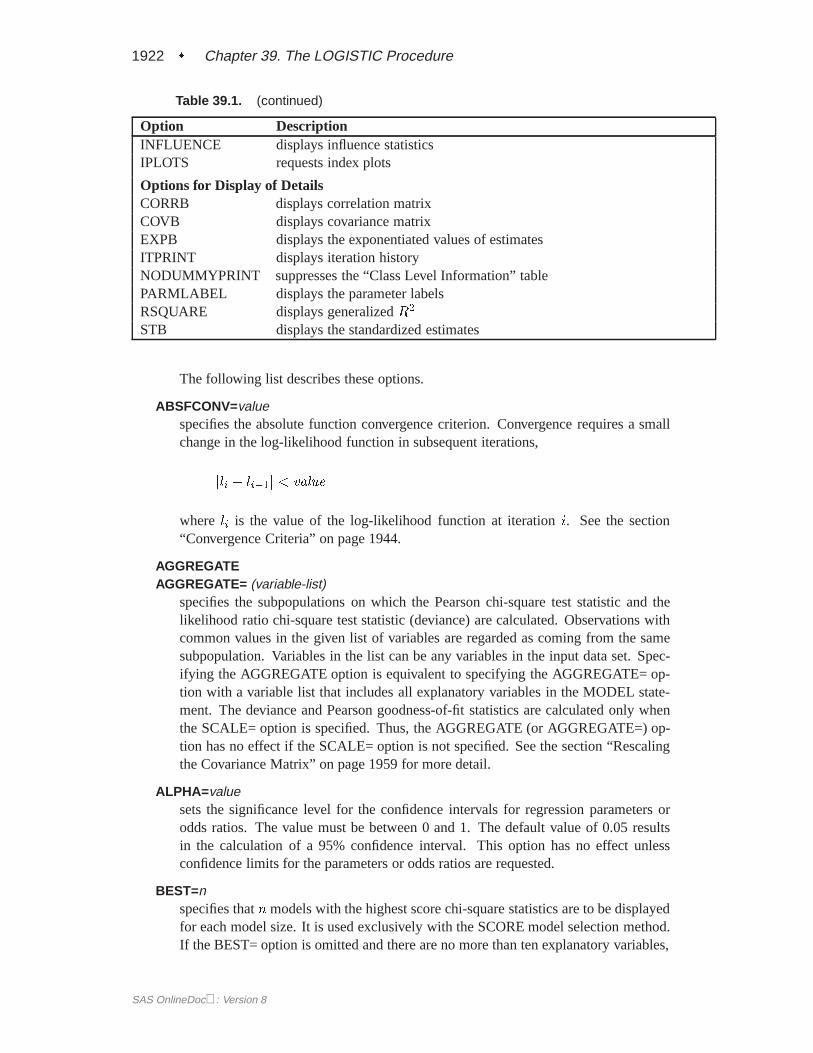
The following list describes these options.
ABSFCONV=valuespecifies the absolute function convergence criterion. Convergence requires a smallchange in the log-likelihood function in subsequent iterations,
jli � li�1j < value
where li is the value of the log-likelihood function at iterationi. See the section“Convergence Criteria” on page 1944.
AGGREGATEAGGREGATE= (variable-list)
specifies the subpopulations on which the Pearson chi-square test statistic and thelikelihood ratio chi-square test statistic (deviance) are calculated. Observations withcommon values in the given list of variables are regarded as coming from the samesubpopulation. Variables in the list can be any variables in the input data set. Spec-ifying the AGGREGATE option is equivalent to specifying the AGGREGATE= op-tion with a variable list that includes all explanatory variables in the MODEL state-ment. The deviance and Pearson goodness-of-fit statistics are calculated only whenthe SCALE= option is specified. Thus, the AGGREGATE (or AGGREGATE=) op-tion has no effect if the SCALE= option is not specified. See the section “Rescalingthe Covariance Matrix” on page 1959 for more detail.
ALPHA= valuesets the significance level for the confidence intervals for regression parameters orodds ratios. The value must be between 0 and 1. The default value of 0.05 resultsin the calculation of a 95% confidence interval. This option has no effect unlessconfidence limits for the parameters or odds ratios are requested.
BEST=nspecifies thatnmodels with the highest score chi-square statistics are to be displayedfor each model size. It is used exclusively with the SCORE model selection method.If the BEST= option is omitted and there are no more than ten explanatory variables,
SAS OnlineDoc: Version 8

MODEL Statement � 1923
then all possible models are listed for each model size. If the option is omitted andthere are more than ten explanatory variables, then the number of models selected foreach model size is, at most, equal to the number of explanatory variables listed in theMODEL statement.
CLODDS=PL | WALD | BOTHrequests confidence intervals for the odds ratios. Computation of these confidence in-tervals is based on the profile likelihood (CLODDS=PL) or based on individual Waldtests (CLODDS=WALD). By specifying CLPARM=BOTH, the procedure computestwo sets of confidence intervals for the odds ratios, one based on the profile likelihoodand the other based on the Wald tests. The confidence coefficient can be specifiedwith the ALPHA= option.
CLPARM=PL | WALD | BOTHrequests confidence intervals for the parameters. Computation of these confidenceintervals is based on the profile likelihood (CLPARM=PL) or individual Wald tests(CLPARM=WALD). By specifying CLPARM=BOTH, the procedure computes twosets of confidence intervals for the parameters, one based on the profile likelihood andthe other based on individual Wald tests. The confidence coefficient can be specifiedwith the ALPHA= option. See the “Confidence Intervals for Parameters” section onpage 1950 for more information.
CONVERGE=valueis the same as specifying the XCONV= option.
CORRBdisplays the correlation matrix of the parameter estimates.
COVBdisplays the covariance matrix of the parameter estimates.
CTABLEclassifies the input binary response observations according to whether the predictedevent probabilities are above or below some cutpoint valuez in the range(0; 1). Anobservation is predicted as an event if the predicted event probability exceedsz. Youcan supply a list of cutpoints other than the default list by using the PPROB= option(page 1928). The CTABLE option is ignored if the data have more than two responselevels. Also, false positive and negative rates can be computed as posterior proba-bilities using Bayes’ theorem. You can use the PEVENT= option to specify priorprobabilities for computing these rates. For more information, see the “ClassificationTable” section on page 1956.
DETAILSproduces a summary of computational details for each step of the variable selectionprocess. It produces the “Analysis of Effects Not in the Model” table before dis-playing the effect selected for entry for FORWARD or STEPWISE selection. Foreach model fitted, it produces the “Type III Analysis of Effects” table if the fittedmodel involves CLASS variables, the “Analysis of Maximum Likelihood Estimates”table, and measures of association between predicted probabilities and observed re-sponses. For the statistics included in these tables, see the “Displayed Output” sectionon page 1969. The DETAILS option has no effect when SELECTION=NONE.
SAS OnlineDoc: Version 8
1924 � Chapter 39. The LOGISTIC Procedure
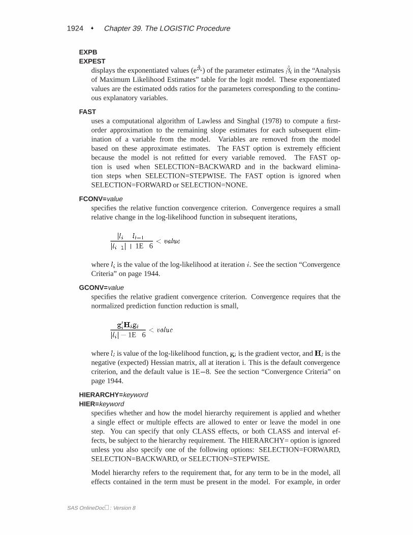
EXPBEXPEST
displays the exponentiated values (e�i) of the parameter estimates�i in the “Analysisof Maximum Likelihood Estimates” table for the logit model. These exponentiatedvalues are the estimated odds ratios for the parameters corresponding to the continu-ous explanatory variables.
FASTuses a computational algorithm of Lawless and Singhal (1978) to compute a first-order approximation to the remaining slope estimates for each subsequent elim-ination of a variable from the model. Variables are removed from the modelbased on these approximate estimates. The FAST option is extremely efficientbecause the model is not refitted for every variable removed. The FAST op-tion is used when SELECTION=BACKWARD and in the backward elimina-tion steps when SELECTION=STEPWISE. The FAST option is ignored whenSELECTION=FORWARD or SELECTION=NONE.
FCONV=valuespecifies the relative function convergence criterion. Convergence requires a smallrelative change in the log-likelihood function in subsequent iterations,
jli � li�1jjli�1j+ 1E�6
< value
whereli is the value of the log-likelihood at iterationi. See the section “ConvergenceCriteria” on page 1944.
GCONV=valuespecifies the relative gradient convergence criterion. Convergence requires that thenormalized prediction function reduction is small,
g0iHigi
jlij+ 1E�6< value
whereli is value of the log-likelihood function,gi is the gradient vector, andHi is thenegative (expected) Hessian matrix, all at iteration i. This is the default convergencecriterion, and the default value is 1E�8. See the section “Convergence Criteria” onpage 1944.
HIERARCHY=keywordHIER=keyword
specifies whether and how the model hierarchy requirement is applied and whethera single effect or multiple effects are allowed to enter or leave the model in onestep. You can specify that only CLASS effects, or both CLASS and interval ef-fects, be subject to the hierarchy requirement. The HIERARCHY= option is ignoredunless you also specify one of the following options: SELECTION=FORWARD,SELECTION=BACKWARD, or SELECTION=STEPWISE.
Model hierarchy refers to the requirement that, for any term to be in the model, alleffects contained in the term must be present in the model. For example, in order
SAS OnlineDoc: Version 8

MODEL Statement � 1925
for the interaction A*B to enter the model, the main effects A and B must be in themodel. Likewise, neither effect A nor B can leave the model while the interactionA*B is in the model.
The keywords you can specify in the HIERARCHY= option are described as follows:
NONE
Model hierarchy is not maintained. Any single effect can enter orleave the model at any given step of the selection process.
SINGLE
Only one effect can enter or leave the model at one time, subject tothe model hierarchy requirement. For example, suppose that youspecify the main effects A and B and the interaction of A*B in themodel. In the first step of the selection process, either A or B canenter the model. In the second step, the other main effect can enterthe model. The interaction effect can enter the model only whenboth main effects have already been entered. Also, before A orB can be removed from the model, the A*B interaction must firstbe removed. All effects (CLASS and interval) are subject to thehierarchy requirement.
SINGLECLASS
This is the same as HIERARCHY=SINGLE except that onlyCLASS effects are subject to the hierarchy requirement.
MULTIPLE
More than one effect can enter or leave the model at one time,subject to the model hierarchy requirement. In a forward selectionstep, a single main effect can enter the model, or an interaction canenter the model together with all the effects that are contained in theinteraction. In a backward elimination step, an interaction itself,or the interaction together with all the effects that the interactioncontains, can be removed. All effects (CLASS and interval) aresubject to the hierarchy requirement.
MULTIPLECLASS
This is the same as HIERARCHY=MULTIPLE except that onlyCLASS effects are subject to the hierarchy requirement.
The default value is HIERARCHY=SINGLE, which means that model hierarchy isto be maintained for all effects (that is, both CLASS and interval effects) and thatonly a single effect can enter or leave the model at each step.
SAS OnlineDoc: Version 8

1926 � Chapter 39. The LOGISTIC Procedure
INCLUDE=nincludes the first n effects in the MODEL statement in every model.By default, INCLUDE=0. The INCLUDE= option has no effect whenSELECTION=NONE.
Note that the INCLUDE= and START= options perform different tasks: theINCLUDE= option includes the firstn effects variables in every model, whereas theSTART= option only requires that the firstn effects appear in the first model.
INFLUENCEdisplays diagnostic measures for identifying influential observations in the case ofa binary response model. It has no effect otherwise. For each observation, theINFLUENCE option displays the case number (which is the sequence number ofthe observation), the values of the explanatory variables included in the final model,and the regression diagnostic measures developed by Pregibon (1981). For a dis-cussion of these diagnostic measures, see the “Regression Diagnostics” section onpage 1963.
IPLOTSproduces an index plot for each regression diagnostic statistic. An index plot is ascatterplot with the regression diagnostic statistic represented on the y-axis and thecase number on the x-axis. See Example 39.4 on page 1998 for an illustration.
ITPRINTdisplays the iteration history of the maximum-likelihood model fitting. The ITPRINToption also displays the last evaluation of the gradient vector and the final change inthe�2 Log Likelihood.
LACKFITLACKFIT<(n)>
performs the Hosmer and Lemeshow goodness-of-fit test (Hosmer and Lemeshow1989) for the case of a binary response model. The subjects are divided into approx-imately ten groups of roughly the same size based on the percentiles of the estimatedprobabilities. The discrepancies between the observed and expected number of ob-servations in these groups are summarized by the Pearson chi-square statistic, whichis then compared to a chi-square distribution witht degrees of freedom, wheret isthe number of groups minusn. By default,n=2. A smallp-value suggests that thefitted model is not an adequate model.
LINK=CLOGLOG | LOGIT | PROBITL=CLOGLOG | LOGIT | PROBIT
specifies the link function for the response probabilities. CLOGLOG is the comple-mentary log-log function, LOGIT is the log odds function, and PROBIT (or NOR-MIT) is the inverse standard normal distribution function. By default, LINK=LOGIT.See the section “Link Functions and the Corresponding Distributions” on page 1940for details.
MAXITER=nspecifies the maximum number of iterations to perform. By default, MAXITER=25.If convergence is not attained inn iterations, the displayed output and all output datasets created by the procedure contain results that are based on the last maximumlikelihood iteration.
SAS OnlineDoc: Version 8

MODEL Statement � 1927
MAXSTEP=nspecifies the maximum number of times any explanatory variable is added to orremoved from the model when SELECTION=STEPWISE. The default number istwice the number of explanatory variables in the MODEL statement. When theMAXSTEP= limit is reached, the stepwise selection process is terminated. All statis-tics displayed by the procedure (and included in output data sets) are based on thelast model fitted. The MAXSTEP= option has no effect when SELECTION=NONE,FORWARD, or BACKWARD.
NOCHECKdisables the checking process to determine whether maximum likelihood estimates ofthe regression parameters exist. If you are sure that the estimates are finite, this optioncan reduce the execution time if the estimation takes more than eight iterations. Formore information, see the “Existence of Maximum Likelihood Estimates” section onpage 1944.
NODUMMYPRINTNODESIGNPRINTNODP
suppresses the “Class Level Information” table, which shows how the design matrixcolumns for the CLASS variables are coded.
NOINTsuppresses the intercept for the binary response model or the first intercept for the or-dinal response model. This can be particularly useful in conditional logistic analysis;see Example 39.9 on page 2026.
NOFITperforms the global score test without fitting the model. The global score test evalu-ates the joint significance of the effects in the MODEL statement. No further analysesare performed. If the NOFIT option is specified along with other MODEL statementoptions, NOFIT takes effect and all other options except LINK=, TECHNIQUE=,and OFFSET= are ignored.
OFFSET= namenames the offset variable. The regression coefficient for this variable will be fixedat 1.
OUTROC=SAS-data-setOUTR=SAS-data-set
creates, for binary response models, an output SAS data set that contains the data nec-essary to produce the receiver operating characteristic (ROC) curve. See the section“OUTROC= Data Set” on page 1968 for the list of variables in this data set.
PARMLABELdisplays the labels of the parameters in the “Analysis of Maximum Likelihood Esti-mates” table.
SAS OnlineDoc: Version 8

1928 � Chapter 39. The LOGISTIC Procedure
PEVENT= valuePEVENT= (list )
specifies one prior probability or a list of prior probabilities for the event of interest.The false positive and false negative rates are then computed as posterior probabili-ties by Bayes’ theorem. The prior probability is also used in computing the rate ofcorrect prediction. For each prior probability in the given list, a classification tableof all observations is computed. By default, the prior probability is the total sampleproportion of events. The PEVENT= option is useful for stratified samples. It has noeffect if the CTABLE option is not specified. For more information, see the section“False Positive and Negative Rates Using Bayes’ Theorem” on page 1957. Also seethe PPROB= option for information on how thelist is specified.
PLCLis the same as specifying CLPARM=PL.
PLCONV= valuecontrols the convergence criterion for confidence intervals based on the profile likeli-hood function. The quantityvaluemust be a positive number, with a default value of1E�4. The PLCONV= option has no effect if profile likelihood confidence intervals(CLPARM=PL) are not requested.
PLRLis the same as specifying CLODDS=PL.
PPROB=valuePPROB= (list )
specifies one critical probability value (or cutpoint) or a list of critical probabilityvalues for classifying observations with the CTABLE option. Eachvalue must bebetween 0 and 1. A response that has a crossvalidated predicted probability greaterthan or equal to the current PPROB= value is classified as an event response. ThePPROB= option is ignored if the CTABLE option is not specified.
A classification table for each of several cutpoints can be requested by specifying alist. For example,
pprob= (0.3, 0.5 to 0.8 by 0.1)
requests a classification of the observations for each of the cutpoints 0.3, 0.5, 0.6, 0.7,and 0.8. If the PPROB= option is not specified, the default is to display the classi-fication for a range of probabilities from the smallest estimated probability (roundedbelow to the nearest 0.02) to the highest estimated probability (rounded above to thenearest 0.02) with 0.02 increments.
RIDGING=ABSOLUTE | RELATIVE | NONEspecifies the technique used to improve the log-likelihood function when its value inthe current iteration is less than that in the previous iteration. If you specify the RIDG-ING=ABSOLUTE option, the diagonal elements of the negative (expected) Hessianare inflated by adding the ridge value. If you specify the RIDGING=RELATIVE op-tion, the diagonal elements are inflated by a factor of 1 plus the ridge value. If youspecify the RIDGING=NONE option, the crude line search method of taking half astep is used instead of ridging. By default, RIDGING=RELATIVE.
SAS OnlineDoc: Version 8

MODEL Statement � 1929
RISKLIMITSRLWALDRL
is the same as specifying CLODDS=WALD.
ROCEPS= numberspecifies the criterion for grouping estimated event probabilities that are close to eachother for the ROC curve. In each group, the difference between the largest and thesmallest estimated event probabilities does not exceed the given value. The defaultis 1E�4. The smallest estimated probability in each group serves as a cutpoint forpredicting an event response. The ROCEPS= option has no effect if the OUTROC=option is not specified.
RSQUARERSQ
requests a generalizedR2 measure for the fitted model. For more information, seethe “Generalized Coefficient of Determination” section on page 1948.
SCALE= scaleenables you to supply the value of the dispersion parameter or to specify the methodfor estimating the dispersion parameter. It also enables you to display the “Devianceand Pearson Goodness-of-Fit Statistics” table. To correct for overdispersion or un-derdispersion, the covariance matrix is multiplied by the estimate of the dispersionparameter. Valid values forscaleare as follows:
D | DEVIANCE specifies that the dispersion parameter be estimated bythe deviance divided by its degrees of freedom.
P | PEARSON specifies that the dispersion parameter be estimated bythe Pearson chi-square statistic divided by its degrees offreedom.
WILLIAMS <( constant)> specifies that Williams’ method be used to modeloverdispersion. This option can be used only with theevents/trialssyntax. An optionalconstantcan be speci-fied as the scale parameter; otherwise, a scale parameteris estimated under the full model. A set of weights iscreated based on this scale parameter estimate. Theseweights can then be used in fitting subsequent mod-els of fewer terms than the full model. When fittingthese submodels, specify the computed scale parameteras constant. See Example 39.8 on page 2021 for anillustration.
N | NONE specifies that no correction is needed for the dispersionparameter; that is, the dispersion parameter remains as1. This specification is used for requesting the devianceand the Pearson chi-square statistic without adjusting foroverdispersion.
SAS OnlineDoc: Version 8

1930 � Chapter 39. The LOGISTIC Procedure
constant sets the estimate of the dispersion parameter to be thesquare of the givenconstant. For example, SCALE=2sets the dispersion parameter to 4. The valueconstantmust be a positive number.
You can use the AGGREGATE (or AGGREGATE=) option to define the subpop-ulations for calculating the Pearson chi-square statistic and the deviance. In theabsence of the AGGREGATE (or AGGREGATE=) option, each observation is re-garded as coming from a different subpopulation. For theevents/trialssyntax, eachobservation consists ofn Bernoulli trials, wheren is the value of thetrials vari-able. Forsingle-trial syntax, each observation consists of a single response, and forthis setting it is not appropriate to carry out the Pearson or deviance goodness-of-fit analysis. Thus, PROC LOGISTIC ignores specifications SCALE=P, SCALE=D,and SCALE=N whensingle-trial syntax is specified without the AGGREGATE (orAGGREGATE=) option.
The “Deviance and Pearson Goodness-of-Fit Statistics” table includes the Pearsonchi-square statistic, the deviance, their degrees of freedom, the ratio of each statisticdivided by its degrees of freedom, and the correspondingp-value. For more informa-tion, see the “Overdispersion” section on page 1958.
SELECTION=BACKWARD | B| FORWARD | F| NONE | N| STEPWISE | S| SCORE
specifies the method used to select the variables in the model. BACKWARD requestsbackward elimination, FORWARD requests forward selection, NONE fits the com-plete model specified in the MODEL statement, and STEPWISE requests stepwiseselection. SCORE requests best subset selection. By default, SELECTION=NONE.For more information, see the “Effect Selection Methods” section on page 1945.
SEQUENTIALSEQ
forces effects to be added to the model in the order specified in the MODEL state-ment or eliminated from the model in the reverse order specified in the MODELstatement. The model-building process continues until the next effect to be added hasan insignificant adjusted chi-square statistic or until the next effect to be deleted hasa significant Wald chi-square statistic. The SEQUENTIAL option has no effect whenSELECTION=NONE.
SINGULAR=valuespecifies the tolerance for testing the singularity of the Hessian matrix (Newton-Raphson algorithm) or the expected value of the Hessian matrix (Fisher-scoring al-gorithm). The Hessian matrix is the matrix of second partial derivatives of the loglikelihood. The test requires that a pivot for sweeping this matrix be at least thisnumber times a norm of the matrix. Values of the SINGULAR= option must benumeric. By default, SINGULAR=1E�12.
SAS OnlineDoc: Version 8

MODEL Statement � 1931
SLENTRY=valueSLE=value
specifies the significance level of the score chi-square for entering an effect into themodel in the FORWARD or STEPWISE method. Values of the SLENTRY= optionshould be between 0 and 1, inclusive. By default, SLENTRY=0.05. The SLENTRY=option has no effect when SELECTION=NONE, SELECTION=BACKWARD, orSELECTION=SCORE.
SLSTAY=valueSLS=value
specifies the significance level of the Wald chi-square for an effect to stay in the modelin a backward elimination step. Values of the SLSTAY= option should be between0 and 1, inclusive. By default, SLSTAY=0.05. The SLSTAY= option has no effectwhen SELECTION=NONE, SELECTION=FORWARD, or SELECTION=SCORE.
START=nbegins the FORWARD, BACKWARD, or STEPWISE effect selection process withthe firstn effects listed in the MODEL statement. The value ofn ranges from 0 tos, wheres is the total number of effects in the MODEL statement. The default valueof n is s for the BACKWARD method and 0 for the FORWARD and STEPWISEmethods. Note that START=n specifies only that the firstn effects appear in thefirst model, while INCLUDE=n requires that the firstn effects be included in everymodel. For the SCORE method, START=n specifies that the smallest models containn effects, wheren ranges from 1 tos; the default value is 1. The START= option hasno effect when SELECTION=NONE.
STBdisplays the standardized estimates for the parameters for the continuous explana-tory variables in the “Analysis of Maximum Likelihood Estimates” table. The stan-dardized estimate of�i is given by�i=(s=si), wheresi is the total sample standarddeviation for theith explanatory variable and
s =
8<:�=p3 Logistic
1 Normal�=p6 Extreme-value
For the intercept parameters and parameters associated with a CLASS variable, thestandardized estimates are set to missing.
STOP=nspecifies the maximum (FORWARD method) or minimum (BACKWARD method)number of effects to be included in the final model. The effect selection process isstopped whenn effects are found. The value ofn ranges from 0 tos, wheres is thetotal number of effects in the MODEL statement. The default value ofn is s for theFORWARD method and 0 for the BACKWARD method. For the SCORE method,START=n specifies that the smallest models containn effects, wheren ranges from1 to s; the default value ofn is s. The STOP= option has no effect when SELEC-TION=NONE or STEPWISE.
SAS OnlineDoc: Version 8

1932 � Chapter 39. The LOGISTIC Procedure
STOPRESSR
specifies that the removal or entry of effects be based on the value of the residualchi-square. If SELECTION=FORWARD, then the STOPRES option adds the effectsinto the model one at a time until the residual chi-square becomes insignificant (untilthe p-value of the residual chi-square exceeds the SLENTRY=value). If SELEC-TION=BACKWARD, then the STOPRES option removes effects from the modelone at a time until the residual chi-square becomes significant (until thep-value ofthe residual chi-square becomes less than the SLSTAY=value). The STOPRES op-tion has no effect when SELECTION=NONE or SELECTION=STEPWISE.
TECHNIQUE=FISHER | NEWTONTECH=FISHER | NEWTON
specifies the optimization technique for estimating the regression parameters.NEWTON (or NR) is the Newton-Raphson algorithm and FISHER (or FS) is theFisher-scoring algorithm. Both techniques yield the same estimates, but the estimatedcovariance matrices are slightly different except for the case when the LOGIT linkis specified for binary response data. The default is TECHNIQUE=FISHER. See thesection “Iterative Algorithms for Model-Fitting” on page 1942 for details.
WALDCLCL
is the same as specifying CLPARM=WALD.
XCONV=valuespecifies the relative parameter convergence criterion. Convergence requires a smallrelative parameter change in subsequent iterations,
maxj
j�(j)i j < value
where
�(j)i =
8<: �(j)i � �
(j)i�1 j�(j)i�1j < 0:01
�(j)i ��
(j)i�1
�(j)i�1
otherwise
and�(j)i is the estimate of thejth parameter at iterationi. See the section “Conver-gence Criteria” on page 1944.
OUTPUT Statement
OUTPUT< OUT=SAS-data-set > < options >;
The OUTPUT statement creates a new SAS data set that contains all the variables inthe input data set and, optionally, the estimated linear predictors and their standard er-ror estimates, the estimates of the cumulative or individual response probabilities, andthe confidence limits for the cumulative probabilities. Regression diagnostic statis-tics and estimates of crossvalidated response probabilities are also available for binary
SAS OnlineDoc: Version 8
OUTPUT Statement � 1933
response models. Formulas for the statistics are given in the “Linear Predictor, Pre-dicted Probability, and Confidence Limits” section on page 1955 and the “RegressionDiagnostics” section on page 1963.
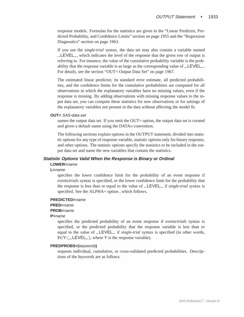
If you use thesingle-trial syntax, the data set may also contain a variable named
–LEVEL–, which indicates the level of the response that the given row of output isreferring to. For instance, the value of the cumulative probability variable is the prob-ability that the response variable is as large as the corresponding value of–LEVEL–.For details, see the section “OUT= Output Data Set” on page 1967.
The estimated linear predictor, its standard error estimate, all predicted probabili-ties, and the confidence limits for the cumulative probabilities are computed for allobservations in which the explanatory variables have no missing values, even if theresponse is missing. By adding observations with missing response values to the in-put data set, you can compute these statistics for new observations or for settings ofthe explanatory variables not present in the data without affecting the model fit.
OUT= SAS-data-setnames the output data set. If you omit the OUT= option, the output data set is createdand given a default name using the DATAn convention.
The following sections explain options in the OUTPUT statement, divided into statis-tic options for any type of response variable, statistic options only for binary response,and other options. The statistic options specify the statistics to be included in the out-put data set and name the new variables that contain the statistics.
Statistic Options Valid When the Response is Binary or OrdinalLOWER=nameL=name
specifies the lower confidence limit for the probability of an event response ifevents/trialssyntax is specified, or the lower confidence limit for the probability thatthe response is less than or equal to the value of–LEVEL– if single-trial syntax isspecified. See the ALPHA= option , which follows.
PREDICTED=namePRED=namePROB=nameP=name
specifies the predicted probability of an event response ifevents/trialssyntax isspecified, or the predicted probability that the response variable is less than orequal to the value of–LEVEL– if single-trial syntax is specified (in other words,Pr(Y�–LEVEL–), whereY is the response variable).
PREDPROBS=(keywords)requests individual, cumulative, or cross-validated predicted probabilities. Descrip-tions of thekeywordsare as follows.
SAS OnlineDoc: Version 8

1934 � Chapter 39. The LOGISTIC Procedure
INDIVIDUAL | I requests the predicted probability of each response level. For aresponse variableY with three levels, 1, 2, and 3, the individualprobabilities are Pr(Y=1), Pr(Y=2), and Pr(Y=3).
CUMULATIVE | C requests the cumulative predicted probability of each responselevel. For a response variableY with three response levels, 1,2,and 3, the cumulative probabilities are Pr(Y�1), Pr(Y�2), andPr(Y�3). The cumulative probability for the last response levelalways has the constant value of 1.
CROSSVALIDATE | XVALIDATE | X requests the cross-validated individual pre-dicted probability of each response level. These probabilities arederived from the leave-one-out principle; that is, dropping the dataof one subject and reestimating the parameter estimates. PROCLOGISTIC uses a less expensive one-step approximation to com-pute the parameter estimates. Note that, for ordinal models, thecross validated probabilities are not computed and are set to miss-ing.
See the end of this section for further details regarding the PREDPROBS= option.
STDXBETA=namespecifies the standard error estimate of XBETA (the definition of which follows).
UPPER=nameU=name
specifies the upper confidence limit for the probability of an event response ifevents/trials modelis specified, or the upper confidence limit for the probability thatthe response is less than or equal to the value of–LEVEL– if single-trial syntax isspecified. See the ALPHA=option mentioned previously.
XBETA=namespecifies the estimate of the linear predictor�i + �0x, wherei is the correspondingordered value of–LEVEL– .
Statistic Options Valid Only When the Response is BinaryC=name
specifies the confidence interval displacement diagnostic that measures the influenceof individual observations on the regression estimates.
CBAR=namespecifies the another confidence interval displacement diagnostic, which measuresthe overall change in the global regression estimates due to deleting an individualobservation.
DFBETAS= –ALL –DFBETAS=var-list
specifies the standardized differences in the regression estimates for assessing the ef-fects of individual observations on the estimated regression parameters in the fittedmodel. You can specify a list of up tos + 1 variable names, wheres is the numberof explanatory variables in the MODEL statement, or you can specify just the key-word–ALL –. In the former specification, the first variable contains the standardized
SAS OnlineDoc: Version 8

OUTPUT Statement � 1935
differences in the intercept estimate, the second variable contains the standardizeddifferences in the parameter estimate for the first explanatory variable in the MODELstatement, and so on. In the latter specification, the DFBETAS statistics are namedDFBETA–xxx , wherexxx is the name of the regression parameter. For example, ifthe model contains two variables X1 and X2, the specification DFBETAS=–ALL –produces three DFBETAS statistics named DFBETA–Intercept, DFBETA–X1, andDFBETA–X2. If an explanatory variable is not included in the final model, the cor-responding output variable named in DFBETAS=var-list contains missing values.
DIFCHISQ=namespecifies the change in the chi-square goodness-of-fit statistic attributable to deletingthe individual observation.
DIFDEV=namespecifies the change in the deviance attributable to deleting the individual observation.
H=namespecifies the diagonal element of the hat matrix for detecting extreme points in thedesign space.
RESCHI=namespecifies the Pearson (Chi) residual for identifying observations that are poorly ac-counted for by the model.
RESDEV=namespecifies the deviance residual for identifying poorly fitted observations.
Other OptionsALPHA= value
sets the confidence level used for the confidence limits for the appropriate responseprobabilities. The quantityvaluemust be between 0 and 1. By default, ALPHA=0.05,which results in the calculation of a 95% confidence interval.
Details of the PREDPROBS= OptionYou can request any of the three given types of predicted probabilities. For example,you can request both the individual predicted probabilities and the cross-validatedprobabilities by specifying PREDPROBS=(I X).
When you specify the PREDPROBS= option, two automatic variables–FROM– and
–INTO– are included for thesingle-trial syntax and only one variable,–INTO– , isincluded for theevents/trialssyntax. The–FROM– variable contains the formattedvalue of the observed response. The variable–INTO– contains the formatted valueof the response level with the largest individual predicted probability.
If you specify PREDPROBS=INDIVIDUAL, the OUTPUT data set containsk addi-tional variables representing the individual probabilities, one for each response level,wherek is the maximum number of response levels across all BY-groups. The namesof these variables have the formIP–xxx, wherexxx represents the particular level.The representation depends on the following situations.
SAS OnlineDoc: Version 8

1936 � Chapter 39. The LOGISTIC Procedure
� If you specifyevents/trialssyntax,xxx is either ‘Event’ or ‘Nonevent’. Thus,the variable containing the event probabilities is namedIP–Event and the vari-able containing the nonevent probabilities is namedIP–Nonevent.
� If you specify thesingle-trial syntax with more than one BY group,xxx is1 for the first ordered level of the response, 2 for the second ordered levelof the response,: : :, and so forth, as given in the “Response Profile” table.The variable containing the predicted probabilities Pr(Y=1) is namedIP–1,whereY is the response variable. Similarly,IP–2 is the name of the variablecontaining the predicted probabilities Pr(Y=2), and so on.
� If you specify thesingle-trial syntax with no BY-group processing,xxx is theleft-justified formatted value of the response level (the value may be truncatedso thatIP–xxx does not exceed 32 characters.) For example, ifY is the re-sponse variable with response levels ‘None’, ‘Mild’, and ‘Severe’, the vari-ables representing individual probabilities Pr(Y=’None’), P(Y=’Mild’), andP(Y=’Severe’) are namedIP–None, IP–Mild, andIP–Severe, respectively.
If you specify PREDPROBS=CUMULATIVE, the OUTPUT data set containsk ad-ditional variables representing the cumulative probabilities, one for each responselevel, wherek is the maximum number of response levels across all BY-groups.The names of these variables have the formCP–xxx, wherexxx represents the par-ticular response level. The naming convention is similar to that given by PRED-PROBS=INDIVIDUAL. The PREDPROBS=CUMULATIVE values are the same asthose output by the PREDICT=keyword, but are arranged in variables on each outputobservation rather than in multiple output observations.
If you specify PREDPROBS=CROSSVALIDATE, the OUTPUT data set containsk additional variables representing the cross-validated predicted probabilities of thek response levels, wherek is the maximum number of response levels across allBY-groups. The names of these variables have the formXP–xxx, wherexxx rep-resents the particular level. The representation is the same as that given by PRED-PROBS=INDIVIDUAL except that for theevents/trialssyntax there are four vari-ables for the cross-validated predicted probabilities instead of two:
XP–EVENT–R1E is the cross validated predicated probability of an event when acurrent event trial is removed.
XP–NONEVENT–R1E is the cross validated predicated probability of a noneventwhen a current event trial is removed.
XP–EVENT–R1N is the cross validated predicated probability of an event when acurrent nonevent trial is removed.
XP–NONEVENT–R1N is the cross validated predicated probability of a noneventwhen a current nonevent trial is removed.
The cross-validated predicted probabilities are precisely those used in the CTABLEoption. Refer to the “Predicted Probability of an Event for Classification” section onpage 1957 for details of the computation.
SAS OnlineDoc: Version 8

TEST Statement � 1937
TEST Statement
< label: > TEST equation1 < , : : : , < equationk >>< /option > ;
The TEST statement tests linear hypotheses about the regression coefficients. TheWald test is used to test jointly the null hypotheses (H0:L� = c) specified in a singleTEST statement.
Eachequationspecifies a linear hypothesis (a row of theL matrix and the corre-sponding element of thec vector); multipleequationsare separated by commas. Thelabel, which must be a valid SAS name, is used to identify the resulting output andshould always be included. You can submit multiple TEST statements.
The form of anequationis as follows:
term <�term : : : > < =�term <�term : : : >>
wheretermis a parameter of the model, or a constant, or a constant times a parameter.For a binary response model, the intercept parameter is named INTERCEPT; for anordinal response model, the intercept parameters are named INTERCEPT, INTER-CEPT2, INTERCEPT3, and so on. When no equal sign appears, the expression is setto 0. The following code illustrates possible uses of the TEST statement:
proc logistic;model y= a1 a2 a3 a4;test1: test intercept + .5 * a2 = 0;test2: test intercept + .5 * a2;test3: test a1=a2=a3;test4: test a1=a2, a2=a3;
run;
Note that the first and second TEST statements are equivalent, as are the third andfourth TEST statements.
You can specify the following option in the TEST statement after a slash(/).
PRINTdisplays intermediate calculations in the testing of the null hypothesisH0:L� =
c. This includesLbV(b�)L0 bordered by(Lb� � c) and [LbV(b�)L0]�1 bordered by[LbV(b�)L0]�1(Lb��c), whereb� is the maximum likelihood estimator of� andbV(b�)is the estimated covariance matrix ofb�.
For more information, see the “Testing Linear Hypotheses about the RegressionCoefficients” section on page 1963.
SAS OnlineDoc: Version 8

1938 � Chapter 39. The LOGISTIC Procedure
UNITS Statement
UNITS independent1 = list1 < . . . independentk = listk >< /option > ;
The UNITS statement enables you to specify units of change for the continuous ex-planatory variables so that customized odds ratios can be estimated. An estimateof the corresponding odds ratio is produced for each unit of change specified for anexplanatory variable. The UNITS statement is ignored for CLASS variables. If theCLODDS= option is specified in the MODEL statement, the corresponding confi-dence limits for the odds ratios are also displayed.
The termindependentis the name of an explanatory variable andlist represents a listof units of change, separated by spaces, that are of interest for that variable. Eachunit of change in a list has one of the following forms:
� number
� SD or�SD
� number* SD
wherenumberis any nonzero number, and SD is the sample standard deviation of thecorresponding independent variable. For example,X = �2 requests an odds ratiothat represents the change in the odds when the variableX is decreased by two units.X = 2�SD requests an estimate of the change in the odds whenX is increased bytwo sample standard deviations.
You can specify the following option in the UNITS statement after a slash(/).
DEFAULT= listgives a list of units of change for all explanatory variables that are not specified inthe UNITS statement. Each unit of change can be in any of the forms describedpreviously. If the DEFAULT= option is not specified, PROC LOGISTIC does notproduce customized odds ratio estimates for any explanatory variable that is not listedin the UNITS statement.
For more information, see the “Odds Ratio Estimation” section on page 1952.
WEIGHT Statement
WEIGHT variable < / option >;
When a WEIGHT statement appears, each observation in the input data set isweighted by the value of the WEIGHT variable. The values of the WEIGHT vari-able can be nonintegral and are not truncated. Observations with negative, zero, ormissing values for the WEIGHT variable are not used in the model fitting. When theWEIGHT statement is not specified, each observation is assigned a weight of 1.
The following option can be added to the WEIGHT statement after a slash (/).
SAS OnlineDoc: Version 8

Response Level Ordering � 1939
NORMALIZENORM
causes the weights specified by the WEIGHT variable to be normalized so that theyadd up to the actual sample size. With this option, the estimated covariance matrix ofthe parameter estimators is invariant to the scale of the WEIGHT variable.
Details
Missing Values
Any observation with missing values for the response, offset, or explanatory variablesis excluded from the analysis. The estimated linear predictor and its standard errorestimate, the fitted probabilities and confidence limits, and the regression diagnosticstatistics are not computed for any observation with missing offset or explanatoryvariable values. However, if only the response value is missing, the linear predictor,its standard error, the fitted individual and cumulative probabilities, and confidencelimits for the cumulative probabilities can be computed and output to a data set usingthe OUTPUT statement.
Response Level Ordering
For binary response data, the default response function modeled is
logit(p) = log
�p
1� p
�wherep is the probability of the response level identified in the “Response Profiles”table in the displayed output as “Ordered Value 1.” Since
logit(p) = �logit(1� p)
the effect of reversing the order of the two values of the response is to change the signsof � and� in the model logit(p) = � + �0x. Response level ordering is importantbecause PROC LOGISTIC always models the probability of response levels withlower Ordered Value.
By default, response levels are assigned to Ordered Values in ascending, sorted order(that is, the lowest level is assigned Ordered Value 1, the next lowest is assigned 2,and so on). There are a number of ways that you can control the sort order of theresponse categories and, therefore, which level is assigned Ordered Value 1. Oneof the most common sets of response levels is {0,1}, with 1 representing the eventfor which the probability is to be modeled. Consider the example whereY takes thevalues 1 and 0 for event and nonevent, respectively, andExposure is the explanatoryvariable. By default, PROC LOGISTIC assigns Ordered Value 1 to response level0, causing the probability of the nonevent to be modeled. There are several ways tochange this. Besides recoding the variableY, you can do the following.
SAS OnlineDoc: Version 8

1940 � Chapter 39. The LOGISTIC Procedure
� specify the DESCENDING option in the PROC LOGISTIC statement, whichreverses the default ordering ofY from (0,1) to (1,0), making 1 (the event) thelevel with Ordered Value 1:
proc logistic descending;model Y=Exposure;
run;
� assign a format toY such that the first formatted value (when the formattedvalues are put in sorted order) corresponds to the event. For this example,Y=1 is assigned formatted value ‘event’ andY=0 is assigned formatted value‘nonevent’. Since ORDER=FORMATTED by default,Y=1 becomes OrderedValue 1.
proc format;value Disease 1=’event’ 0=’nonevent’;
run;proc logistic;
model Y=Exposure;format Y Disease.;
run;
Link Functions and the Corresponding Distributions
Three link functions are available in the LOGISTIC procedure. The logit function isthe default. To specify a different link function, use the LINK= option in the MODELstatement. The link functions and the corresponding distributions are as follows:
� The logit function
g(p) = log(p=(1 � p))
is the inverse of the cumulative logistic distribution function, which is
F (x) = 1=(1 + exp(�x))
� The probit (or normit) function
g(p) = ��1(p)
is the inverse of the cumulative standard normal distribution function, which is
F (x) = �(x) = (2�)�1=2Z x
�1
exp(�z2=2)dz
Traditionally, the probit function contains the additive constant 5, but through-out PROC LOGISTIC, the terms probit and normit are used interchangeably.
SAS OnlineDoc: Version 8

Determining Observations for Likelihood Contributions � 1941
� The complementary log-log function
g(p) = log(� log(1� p))
is the inverse of the cumulative extreme-value function (also called the Gom-pertz distribution), which is
F (x) = 1� exp(� exp(x))
The variances of these three corresponding distributions are not the same. Theirrespective means and variances are
Distribution Mean VarianceNormal 0 1Logistic 0 �2=3Extreme-value � �2=6
where is the Euler constant. In comparing parameter estimates using different linkfunctions, you need to take into account the different scalings of the correspondingdistributions and, for the complementary log-log function, a possible shift in location.For example, if the fitted probabilities are in the neighborhood of 0.1 to 0.9, then theparameter estimates using the logit link function should be about�=
p3 larger than
the estimates from the probit link function.
Determining Observations for Likelihood Contributions
Suppose the response variable can take on the ordered values1; : : : ; k; k + 1 wherek is an integer� 1. If you useevents/trialssyntax, each observation is split into twoobservations. One has response value 1 with a frequency equal to the frequency of theoriginal observation (which is 1 if the FREQ statement is not used) times the valueof the eventsvariable. The other observation has response value 2 and a frequencyequal to the frequency of the original observation times the value of (trials � events).These two observations will have the same explanatory variable values and the sameFREQ and WEIGHT values as the original observation.
For eithersingle-trial or events/trialssyntax, letj index all observations. In otherwords, forsingle-trialsyntax,j indexes the actual observations. And, forevents/trialssyntax,j indexes the observations after splitting (as described previously). If yourdata set has 30 observations and you usesingle-trial syntax,j has values from 1 to30; if you useevents/trialssyntax,j has values from 1 to 60.
SAS OnlineDoc: Version 8

1942 � Chapter 39. The LOGISTIC Procedure
The likelihood for thejth observation with ordered response valueyj and explanatoryvariables vectorxj is given by
lj =
8<:F (�1 + �0xj) yj = 1F (�i + �0xj)� F (�i�1 + �0xj) 1 < yj = i � k1� F (�k + �0xj) yj = k + 1
whereF (:) is the logistic, normal, or extreme-value distribution function,�1; : : : ; �kare intercept parameters, and� is the slope parameter vector.
Iterative Algorithms for Model-Fitting
Two iterative maximum likelihood algorithms are available in PROC LOGISTIC.The default is the Fisher-scoring method, which is equivalent to fitting by iterativelyreweighted least squares. The alternative algorithm is the Newton-Raphson method.Both algorithms give the same parameter estimates; however, the estimated covari-ance matrix of the parameter estimators may differ slightly. This is due to the factthat the Fisher-scoring method is based on the expected information matrix while theNewton-Raphson method is based on the observed information matrix. In the case ofa binary logit model, the observed and expected information matrices are identical,resulting in identical estimated covariance matrices for both algorithms. You can usethe TECHNIQUE= option to select a fitting algorithm.
Iteratively Reweighted Least-Squares AlgorithmConsider the multinomial variableZj = (Z1j ; : : : ; Z(k+1)j)
0 such that
Zij =
�1 if Yj = i0 otherwise
With pij denoting the probability that thejth observation has response valuei, theexpected value ofZj ispj = (p1j; : : : ; p(k+1)j)
0. The covariance matrix ofZj isVj,which is the covariance matrix of a multinomial random variable for one trial withparameter vectorpj . Let be the vector of regression parameters; in other words, 0 = (�1; : : : ; �k;�
0). And letDj be the matrix of partial derivatives ofpj withrespect to . The estimating equation for the regression parameters is
Xj
D0jWj(Zj � pj) = 0
whereWj = wjfjV�j , wj andfj are the WEIGHT and FREQ values of thejth
observation, andV�j is a generalized inverse ofVj . PROC LOGISTIC choosesV�
j
as the inverse of the diagonal matrix withpj as the diagonal.
SAS OnlineDoc: Version 8

Iterative Algorithms for Model-Fitting � 1943
With a starting value of 0, the maximum likelihood estimate of is obtained itera-tively as
m+1 = m + (Xj
D0jWjDj)
�1Xj
D0jWj(Zj � pj)
whereDj, Wj , andpj are evaluated at m. The expression after the plus sign isthe step size. If the likelihood evaluated at m+1 is less than that evaluated at m,then m+1 is recomputed by step-halving or ridging. The iterative scheme continuesuntil convergence is obtained, that is, until m+1 is sufficiently close to m. Thenthe maximum likelihood estimate of is = m+1.
The covariance matrix of is estimated by
ccov( ) = (Xj
D0jWjDj)
�1
whereDj andWj are, respectively,Dj andWj evaluated at .
By default, starting values are zero for the slope parameters, and for the interceptparameters, starting values are the observed cumulative logits (that is, logits of theobserved cumulative proportions of response). Alternatively, the starting values maybe specified with the INEST= option.
Newton-Raphson AlgorithmWith parameter vector 0 = (�1; : : :; �k;�
0), the gradient vector and the Hessianmatrix are given, respectively, by
g =Xj
wjfj@lj@
H =Xj
�wjfj@2lj@ 2
With a starting value of 0, the maximum likelihood estimate of is obtainediteratively until convergence is obtained:
m+1 = m +H�1 mg m
If the likelihood evaluated at m+1 is less than that evaluated at m, then m+1 isrecomputed by step-halving or ridging.
The covariance matrix of is estimated by
ccov( ) = H�1
SAS OnlineDoc: Version 8

1944 � Chapter 39. The LOGISTIC Procedure
Convergence Criteria
Four convergence criteria are allowed, namely, ABSFCONV=, FCONV=, GCONV=,and XCONV=. If you specify more than one convergence criterion, the optimizationis terminated as soon as one of the criteria is satisfied. If none of the criteria isspecified, the default is GCONV=1E�8.
Existence of Maximum Likelihood Estimates
The likelihood equation for a logistic regression model does not always have a finitesolution. Sometimes there is a nonunique maximum on the boundary of the parameterspace, at infinity. The existence, finiteness, and uniqueness of maximum likelihoodestimates for the logistic regression model depend on the patterns of data points inthe observation space (Albert and Anderson 1984; Santner and Duffy 1986).
Consider a binary response model. LetYj be the response of theith subject andlet xj be the vector of explanatory variables (including the constant 1 associatedwith the intercept). There are three mutually exclusive and exhaustive types of dataconfigurations: complete separation, quasi-complete separation, and overlap.
Complete Separation There is a complete separation of data points if thereexists a vectorb that correctly allocates all observa-tions to their response groups; that is,�
b0xj > 0 Yj = 1b0xj < 0 Yj = 2
This configuration gives nonunique infinite estimates.If the iterative process of maximizing the likelihoodfunction is allowed to continue, the log likelihood di-minishes to zero, and the dispersion matrix becomesunbounded.
Quasi-Complete Separation The data are not completely separable but there is avectorb such that�
b0xj � 0 Yj = 1b0xj � 0 Yj = 2
and equality holds for at least one subject in eachresponse group. This configuration also yields non-unique infinite estimates. If the iterative process ofmaximizing the likelihood function is allowed to con-tinue, the dispersion matrix becomes unbounded andthe log likelihood diminishes to a nonzero constant.
Overlap If neither complete nor quasi-complete separation ex-ists in the sample points, there is an overlap of samplepoints. In this configuration, the maximum likelihoodestimates exist and are unique.
SAS OnlineDoc: Version 8

Effect Selection Methods � 1945
Complete separation and quasi-complete separation are problems typically encoun-tered with small data sets. Although complete separation can occur with any type ofdata, quasi-complete separation is not likely with truly continuous explanatory vari-ables.
The LOGISTIC procedure uses a simple empirical approach to recognize the dataconfigurations that lead to infinite parameter estimates. The basis of this approach isthat any convergence method of maximizing the log likelihood must yield a solutiongiving complete separation, if such a solution exists. In maximizing the log likeli-hood, there is no checking for complete or quasi-complete separation if convergenceis attained in eight or fewer iterations. Subsequent to the eighth iteration, the proba-bility of the observed response is computed for each observation. If the probabilityof the observed response is one for all observations, there is a complete separationof data points and the iteration process is stopped. If the complete separation of datahas not been determined and an observation is identified to have an extremely largeprobability (�0.95) of the observed response, there are two possible situations. First,there is overlap in the data set, and the observation is an atypical observation of itsown group. The iterative process, if allowed to continue, will stop when a maxi-mum is reached. Second, there is quasi-complete separation in the data set, and theasymptotic dispersion matrix is unbounded. If any of the diagonal elements of thedispersion matrix for the standardized observations vectors (all explanatory variablesstandardized to zero mean and unit variance) exceeds 5000, quasi-complete separa-tion is declared and the iterative process is stopped. If either complete separation orquasi-complete separation is detected, a warning message is displayed in the proce-dure output.
Checking for quasi-complete separation is less foolproof than checking for completeseparation. The NOCHECK option in the MODEL statement turns off the processof checking for infinite parameter estimates. In cases of complete or quasi-completeseparation, turning off the checking process typically results in the procedure fail-ing to converge. The presence of a WEIGHT statement also turns off the checkingprocess.
Effect Selection Methods
Five effect-selection methods are available. The simplest method (and the default)is SELECTION=NONE, for which PROC LOGISTIC fits the complete model asspecified in the MODEL statement. The other four methods are FORWARD forforward selection, BACKWARD for backward elimination, STEPWISE for stepwiseselection, and SCORE for best subsets selection. These methods are specified withthe SELECTION= option in the MODEL statement. Intercept parameters are forcedto stay in the model unless the NOINT option is specified.
When SELECTION=FORWARD, PROC LOGISTIC first estimates parameters foreffects forced into the model. These effects are the intercepts and the firstn ex-planatory effects in the MODEL statement, wheren is the number specified by theSTART= or INCLUDE= option in the MODEL statement (n is zero by default). Next,the procedure computes the score chi-square statistic for each effect not in the modeland examines the largest of these statistics. If it is significant at the SLENTRY=
SAS OnlineDoc: Version 8

1946 � Chapter 39. The LOGISTIC Procedure
level, the corresponding effect is added to the model. Once an effect is entered inthe model, it is never removed from the model. The process is repeated until none ofthe remaining effects meet the specified level for entry or until the STOP= value isreached.
When SELECTION=BACKWARD, parameters for the complete model as specifiedin the MODEL statement are estimated unless the START= option is specified. In thatcase, only the parameters for the intercepts and the firstn explanatory effects in theMODEL statement are estimated, wheren is the number specified by the START=option. Results of the Wald test for individual parameters are examined. The leastsignificant effect that does not meet the SLSTAY= level for staying in the model is re-moved. Once an effect is removed from the model, it remains excluded. The processis repeated until no other effect in the model meets the specified level for removal oruntil the STOP= value is reached. Backward selection is often less successful thanforward or stepwise selection because the full model fit in the first step is the modelmost likely to result in a complete or quasi-complete separation of response values asdescribed in the previous section.
The SELECTION=STEPWISE option is similar to the SELECTION=FORWARDoption except that effects already in the model do not necessarily remain. Effectsare entered into and removed from the model in such a way that each forward selec-tion step may be followed by one or more backward elimination steps. The stepwiseselection process terminates if no further effect can be added to the model or if the ef-fect just entered into the model is the only effect removed in the subsequent backwardelimination.
For SELECTION=SCORE, PROC LOGISTIC uses the branch and bound algorithmof Furnival and Wilson (1974) to find a specified number of models with the highestlikelihood score (chi-square) statistic for all possible model sizes, from 1, 2, 3 effectmodels, and so on, up to the single model containing all of the explanatory effects.The number of models displayed for each model size is controlled by the BEST=option. You can use the START= option to impose a minimum model size, and youcan use the STOP= option to impose a maximum model size. For instance, withBEST=3, START=2, and STOP=5, the SCORE selection method displays the bestthree models (that is, the three models with the highest score chi-squares) containing2, 3, 4, and 5 effects. The SELECTION=SCORE option is not available for modelswith CLASS variables.
The options FAST, SEQUENTIAL, and STOPRES can alter the default criteria forentering or removing effects from the model when they are used with the FORWARD,BACKWARD, or STEPWISE selection methods.
SAS OnlineDoc: Version 8

Model Fitting Information � 1947
Model Fitting Information
Suppose the model containss explanatory effects. For thejth observation, letpj bethe estimated probability of the observed response. The three criteria displayed bythe LOGISTIC procedure are calculated as follows:
� �2 Log Likelihood:
�2 Log L = �2Xj
wjfj log(pj)
wherewj andfj are the weight and frequency values of thejth observation.For binary response models usingevents/trialssyntax, this is equivalent to
�2 Log L = �2Xj
wjfjfrj log(pj) + (nj � rj) log(1� pj)g
whererj is the number of events,nj is the number of trials, andpj is theestimated event probability.
� Akaike Information Criterion:
AIC = �2 Log L + 2(k + s)
wherek is the total number of response levels minus one, ands is the numberof explanatory effects.
� Schwarz Criterion:
SC= �2 Log L + (k + s) log(Xj
fj)
wherek ands are as defined previously.
The�2 Log Likelihood statistic has a chi-square distribution under the null hypothe-sis (that all the explanatory effects in the model are zero) and the procedure producesa p-value for this statistic. The AIC and SC statistics give two different ways of ad-justing the�2 Log Likelihood statistic for the number of terms in the model and thenumber of observations used. These statistics should be used when comparing differ-ent models for the same data (for example, when you use the METHOD=STEPWISEoption in the MODEL statement); lower values of the statistic indicate a more desir-able model.
SAS OnlineDoc: Version 8

1948 � Chapter 39. The LOGISTIC Procedure
Generalized Coefficient of Determination
Cox and Snell (1989, pp. 208–209) propose the following generalization of the coef-ficient of determination to a more general linear model:
R2 = 1��L(0)
L(b�)� 2
n
whereL(0) is the likelihood of the intercept-only model,L(b�) is the likelihood ofthe specified model, andn is the sample size. The quantityR2 achieves a maximumof less than one for discrete models, where the maximum is given by
R2max = 1� fL(0)g 2
n
Nagelkerke (1991) proposes the following adjusted coefficient, which can achieve amaximum value of one:
~R2 =R2
R2max
Properties and interpretation ofR2 and ~R2 are provided in Nagelkerke (1991). In the“Testing Global Null Hypothesis: BETA=0” table,R2 is labeled as “RSquare” and~R2 is labeled as “Max-rescaled RSquare.” Use the RSQUARE option to requestR2
and ~R2.
Score Statistics and Tests
To understand the general form of the score statistics, letU( )be the vector of firstpartial derivatives of the log likelihood with respect to the parameter vector , and letH( ) be the matrix of second partial derivatives of the log likelihood with respect to . That is,U( ) is the gradient vector, andH( ) is the Hessian matrix. LetI( ) beeither�H( ) or the expected value of�H( ). Consider a null hypothesisH0. Let 0 be the MLE of underH0. The chi-square score statistic for testingH0 is definedby
U0( 0)I�1( 0)U( 0)
and it has an asymptotic�2 distribution withr degrees of freedom underH0, wherer is the number of restrictions imposed on byH0.
Residual Chi-SquareWhen you use SELECTION=FORWARD, BACKWARD, or STEPWISE, the pro-cedure calculates a residual score chi-square score statistic and reports the statistic,its degrees of freedom, and thep-value. This section describes how the statistic iscalculated.
SAS OnlineDoc: Version 8

Score Statistics and Tests � 1949
Suppose there ares explanatory effects of interest. The full model has a parametervector
= (�1; : : : ; �k; �1; : : : ; �s)0
where�1; : : : ; �k are intercept parameters, and�1; : : : ; �s are slope parameters forthe explanatory effects. Consider the null hypothesisH0:�t+1 = : : : = �s = 0where t < s. For the reduced model witht explanatory effects, let�1; : : : ; �k be theMLEs of the unknown intercept parameters, and let�1; : : : ; �t be the MLEs of theunknown slope parameters. The residual chi-square is the chi-square score statistictesting the null hypothesisH0; that is, the residual chi-square is
U0( 0)I�1( 0)U( 0)
where 0 = (�1; : : : ; �k; �1; : : : ; �t; 0; : : : ; 0)0.
The residual chi-square has an asymptotic chi-square distribution withs� t degreesof freedom. A special case is the global score chi-square, where the reduced modelconsists of thek intercepts and no explanatory effects. The global score statisticis displayed in the “Model-Fitting Information and Testing Global Null HypothesisBETA=0” table. The table is not produced when the NOFIT option is used, but theglobal score statistic is displayed.
Testing Individual Effects Not in the ModelThese tests are performed in the FORWARD or STEPWISE method. In the displayedoutput, the tests are labeled “Score Chi-Square” in the “Analysis of Effects Not in theModel” table and in the “Summary of Stepwise (Forward) Procedure” table. Thissection describes how the tests are calculated.
Suppose thatk intercepts andt explanatory variables (sayv1; : : : ; vt) have been fittedto a model and thatvt+1 is another explanatory variable of interest. Consider a fullmodel with thek intercepts andt + 1 explanatory variables (v1; : : : ; vt; vt+1) and areduced model withvt+1 excluded. The significance ofvt+1 adjusted forv1; : : : ; vtcan be determined by comparing the corresponding residual chi-square with a chi-square distribution with one degree of freedom.
Testing the Parallel Lines AssumptionFor an ordinal response, PROC LOGISTIC performs a test of the parallel lines as-sumption. In the displayed output, this test is labeled “Score Test for the EqualSlopes Assumption” when the LINK= option is NORMIT or CLOGLOG. WhenLINK=LOGIT, the test is labeled as “Score Test for the Proportional Odds Assump-tion” in the output. This section describes the methods used to calculate the test.
SAS OnlineDoc: Version 8
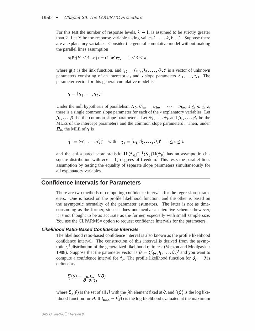
1950 � Chapter 39. The LOGISTIC Procedure
For this test the number of response levels,k + 1, is assumed to be strictly greaterthan 2. Let Y be the response variable taking values1; : : : ; k; k + 1. Suppose thereares explanatory variables. Consider the general cumulative model without makingthe parallel lines assumption
g(Pr(Y � i j x)) = (1;x0) i; 1 � i � k
where g(.) is the link function, and i = (�i; �i1; : : : ; �is)0 is a vector of unknown
parameters consisting of an intercept�i and s slope parameters�i1; : : : ; �is. Theparameter vector for this general cumulative model is
= ( 01; : : : ; 0k)0
Under the null hypothesis of parallelismH0:�1m = �2m = � � � = �km; 1 � m � s,there is a single common slope parameter for each of thes explanatory variables. Let�1; : : :; �s be the common slope parameters. Let�1; : : : ; �k and �1; : : : ; �s be theMLEs of the intercept parameters and the common slope parameters . Then, underH0, the MLE of is
0 = ( 01; : : : ; 0k)0 with i = (�i; �1; : : : ; �s)
0 1 � i � k
and the chi-squared score statisticU0( 0)I�1( 0)U( 0) has an asymptotic chi-
square distribution withs(k � 1) degrees of freedom. This tests the parallel linesassumption by testing the equality of separate slope parameters simultaneously forall explanatory variables.
Confidence Intervals for Parameters
There are two methods of computing confidence intervals for the regression param-eters. One is based on the profile likelihood function, and the other is based onthe asymptotic normality of the parameter estimators. The latter is not as time-consuming as the former, since it does not involve an iterative scheme; however,it is not thought to be as accurate as the former, especially with small sample size.You use the CLPARMS= option to request confidence intervals for the parameters.
Likelihood Ratio-Based Confidence IntervalsThe likelihood ratio-based confidence interval is also known as the profile likelihoodconfidence interval. The construction of this interval is derived from the asymp-totic �2 distribution of the generalized likelihood ratio test (Venzon and Moolgavkar1988). Suppose that the parameter vector is� = (�0; �1; : : : ; �s)
0 and you want tocompute a confidence interval for�j . The profile likelihood function for�j = � isdefined as
l�j (�) = max�2Bj(�)
l(�)
whereBj(�) is the set of all� with thejth element fixed at�, andl(�) is the log like-lihood function for�. If lmax = l(b�) is the log likelihood evaluated at the maximum
SAS OnlineDoc: Version 8

Confidence Intervals for Parameters � 1951
likelihood estimateb�, then2(lmax�l�j (�j)) has a limiting chi-square distribution withone degree of freedom if�j is the true parameter value. Letl0 = lmax � :5�21��;1,where�21��;1 is the100(1 � �) percentile of the chi-square distribution with onedegree of freedom. A100(1 � �)% confidence interval for�j is
f� : l�j (�) � l0g
The endpoints of the confidence interval are found by solving numerically for valuesof �j that satisfy equality in the preceding relation. To obtain an iterative algorithmfor computing the confidence limits, the log likelihood function in a neighborhood of� is approximated by the quadratic function
~l(� + �) = l(�) + �0g +1
2�0V�
whereg = g(�) is the gradient vector andV = V(�) is the Hessian matrix. Theincrement� for the next iteration is obtained by solving the likelihood equations
d
d�f~l(� + �) + �(e0j� � �)g = 0
where� is the Lagrange multiplier,ej is the jth unit vector, and� is an unknownconstant. The solution is
� = �V�1(g + �ej)
By substituting this� into the equation~l(� + �) = l0, you can estimate� as
� = ��2(l0 � l(�) + 1
2g0V�1g)
e0jV�1ej
� 12
The upper confidence limit for�j is computed by starting at the maximum likelihoodestimate of� and iterating with positive values of� until convergence is attained.The process is repeated for the lower confidence limit using negative values of�.
Convergence is controlled by value� specified with the PLCONV= option in theMODEL statement (the default value of� is 1E�4). Convergence is declared on thecurrent iteration if the following two conditions are satisfied:
jl(�)� l0j � �
and
(g + �ej)0V�1(g + �ej) � �
SAS OnlineDoc: Version 8

1952 � Chapter 39. The LOGISTIC Procedure
Wald Confidence IntervalsWald confidence intervals are sometimes called the normal confidence intervals. Theyare based on the asymptotic normality of the parameter estimators. The100(1��)%Wald confidence interval for�j is given byb�j � z1��=2b�jwherezp is the100pth percentile of the standard normal distribution,b�j is the maxi-
mum likelihood estimate of�j , andb�j is the standard error estimate ofb�j .Odds Ratio Estimation
Consider a dichotomous response variable with outcomeseventandnonevent. Con-sider a dichotomous risk factor variable X that takes the value 1 if the risk factor ispresent and 0 if the risk factor is absent. According to the logistic model, the log oddsfunction,g(X), is given by
g(X) � log
�Pr(event j X)
Pr(nonevent j X)
�= �0 + �1X
The odds ratio is defined as the ratio of the odds for those with the risk factor(X = 1) to the odds for those without the risk factor (X = 0). The log of the oddsratio is given by
log( ) � log( (X = 1;X = 0)) = g(X = 1)� g(X = 0) = �1
The parameter,�1, associated with X represents the change in the log odds fromX = 0 toX = 1. So, the odds ratio is obtained by simply exponentiating the valueof the parameter associated with the risk factor. The odds ratio indicates how the oddsof eventchange as you changeX from 0 to 1. For instance, = 2 means that theodds of an event whenX = 1 are twice the odds of an event whenX = 0.
Suppose the values of the dichotomous risk factor are coded as constantsa and binstead of 0 and 1. The odds whenX = a becomeexp(�0+a�1), and the odds whenX = b becomeexp(�0 + b�1). The odds ratio corresponding to an increase inXfrom a to b is
= exp[(b� a)�1] = [exp(�1)]b�a � [exp(�1)]
c
Note that for anya and b such thatc = b � a = 1; = exp(�1). So the oddsratio can be interpreted as the change in the odds for any increase of one unit in thecorresponding risk factor. However, the change in odds for some amount other thanone unit is often of greater interest. For example, a change of one pound in bodyweight may be too small to be considered important, while a change of 10 poundsmay be more meaningful. The odds ratio for a change inX from a to b is estimatedby raising the odds ratio estimate for a unit change inX to the power ofc = b� a asshown previously.
SAS OnlineDoc: Version 8

Odds Ratio Estimation � 1953
For a polytomous risk factor, the computation of odds ratios depends on how the riskfactor is parameterized. For illustration, suppose thatRace is a risk factor with fourcategories:White,Black,Hispanic, andOther.
For the effect parameterization scheme (PARAM=EFFECT) withWhite as the ref-erence group, the design variables forRace are as follows.
Design VariablesRace X1 X2 X3
Black 1 0 0Hispanic 0 1 0
Other 0 0 1White �1 �1 �1
The log odds forBlack is
g(Black) = �0 + �1(X1 = 1) + �2(X2 = 0) + �3(X3 = 0)
= �0 + �1
The log odds forWhite is
g(White) = �0 + �1(X1 = �1) + �2(X2 = �1) + �3(X3 = �1))= �0 � �1 � �2 � �3
Therefore, the log odds ratio ofBlack versusWhite becomes
log( (Black;White)) = g(Black) � g(White)
= 2�1 + �2 + �3
For the reference cell parameterization scheme (PARAM=REF) withWhite as thereference cell, the design variables for race are as follows.
Design VariablesRace X1 X2 X3
Black 1 0 0Hispanic 0 1 0
Other 0 0 1White 0 0 0
The log odds ratio ofBlack versusWhite is given by
log( (Black;White))
= g(Black) � g(White)
= (�0 + �1(X1 = 1) + �2(X2 = 0)) + �3(X3 = 0))�(�0 + �1(X1 = 0) + �2(X2 = 0) + �3(X3 = 0))
= �1
SAS OnlineDoc: Version 8

1954 � Chapter 39. The LOGISTIC Procedure
For the GLM parameterization scheme (PARAM=GLM), the design variables are asfollows.
Design VariablesRace X1 X2 X3 X4
Black 1 0 0 0Hispanic 0 1 0 0
Other 0 0 1 0White 0 0 0 1
The log odds ratio ofBlack versusWhite is
log( (Black;White))
= g(Black) � g(White)
= (�0 + �1(X1 = 1) + �2(X2 = 0) + �3(X3 = 0) + �4(X4 = 0))�(�0 + �1(X1 = 0) + �2(X2 = 0) + �3(X3 = 0) + �4(X4 = 0))
= �1
Consider the hypothetical example of heart disease among race in Hosmer andLemeshow (1989, p 44). The entries in the following contingency table representcounts.
RaceDisease Status White Black Hispanic Other
Present 5 20 15 10Absent 20 10 10 10
The computation of odds ratio ofBlack versusWhite for various parameterizationschemes is tabulated in the following table.
Odds Ratio of Heart Disease ComparingBlack toWhite
Parameter EstimatesPARAM �1 �2 �3 �4 Odds Ratio EstimationEFFECT 0.7651 0.4774 0.0719 exp(2� 0:7651 + 0:4774 + 0:0719) = 8REF 2.0794 1.7917 1.3863 exp(2:0794) = 8GLM 2.0794 1.7917 1.3863 0.0000exp(2:0794) = 8
Since the log odds ratio (log( )) is a linear function of the parameters, the Waldconfidence interval forlog( ) can be derived from the parameter estimates and theestimated covariance matrix. Confidence intervals for the odds ratios are obtainedby exponentiating the corresponding confidence intervals for the log odd ratios. Inthe displayed output of PROC LOGISTIC, the “Odds Ratio Estimates” table containsthe odds ratio estimates and the corresponding 95% Wald confidence intervals. Forcontinuous explanatory variables, these odds ratios correspond to a unit increase inthe risk factors.
SAS OnlineDoc: Version 8

Linear Predictor, Predicted Probability, and Confidence Limits � 1955
To customize odds ratios for specific units of change for a continuous risk factor, youcan use the UNITS statement to specify a list of relevant units for each explanatoryvariable in the model. Estimates of these customized odds ratios are given in a sepa-rate table. Let(Lj ; Uj) be a confidence interval forlog( ). The corresponding lowerand upper confidence limits for the customized odds ratioexp(c�j) areexp[cLj ] andexp[cUj ], respectively (forc > 0), orexp[cUj ] andexp[cLj ], respectively (forc < 0).You use the CLODDS= option to request the confidence intervals for the odds ratios.
Rank Correlation of Observed Responses and PredictedProbabilities
Define an event response as the response having Ordered Value of 1. A pair of ob-servations with different responses is said to be concordant (discordant) if the ob-servation with the response that has the larger Ordered Value has the lower (higher)predicted event probability. If a pair of observations with different responses is nei-ther concordant nor discordant, it is a tie. Enumeration of the total numbers of con-cordant and discordant pairs is carried out by categorizing the predicted probabilitiesinto intervals of length 0.002 and accumulating the corresponding frequencies of ob-servations.
LetN be the sum of observation frequencies in the data. Suppose there is a total oftpairs with different responses,nc of them are concordant,nd of them are discordant,and t � nc � nd of them are tied. PROC LOGISTIC computes the following fourindices of rank correlation for assessing the predictive ability of a model:
c = (nc + 0:5(t � nc � nd))=t
Somers’D = (nc � nd)=t
Goodman-Kruskal Gamma= (nc � nd)=(nc + nd)
Kendall’s Tau-a = (nc � nd)=(0:5N(N � 1))
Note thatc also gives the area under the receiver operating characteristic (ROC) curvewhen the response is binary (Hanley and McNeil 1982).
Linear Predictor, Predicted Probability, and Confidence Limits
This section describes how predicted probabilities and confidence limits arecalculated using the maximum likelihood estimates (MLEs) obtained fromPROC LOGISTIC. For a specific example, see the “Getting Started” section onpage 1906. Predicted probabilities and confidence limits can be output to a data setwith the OUTPUT statement.
SAS OnlineDoc: Version 8

1956 � Chapter 39. The LOGISTIC Procedure
For a vector of explanatory variablesx, the linear predictor
�i = g(Pr(Y � i j x)) = �i + �0x 1 � i � k
is estimated by
�i = �i + �0x
where�i and� are the MLEs of�i and�. The estimated standard error of�i is �(�i),which can be computed as the square root of the quadratic form(1;x0)Vb(1;x
0)0
whereVb is the estimated covariance matrix of the parameter estimates. The asymp-totic 100(1 � �)% confidence interval for�i is given by
�i � z�=2�(�i)
wherez�=2 is the100(1 � �=2) percentile point of a standard normal distribution.
The predicted value and the100(1 � �)% confidence limits for Pr(Y�i j x) areobtained by back-transforming the corresponding measures for the linear predictor.
Link Predicted Probability 100(1-0.5�)%Confidence Limits
LOGIT 1=(1 + e��i) 1=(1 + e��i�z�=2�(�i))
PROBIT �(�i) �(�i � z�=2�(�i))
CLOGLOG 1� e�e�i 1� e�e�i�z�=2�(�i)
Classification Table
For binary response data, the response is either anevent or a nonevent. InPROC LOGISTIC, the response with Ordered Value 1 is regarded as theevent, andthe response with Ordered Value 2 is thenonevent. PROC LOGISTIC models theprobability of theevent. From the fitted model, a predictedeventprobability can becomputed for each observation. The method to compute a reduced-bias estimate ofthe predicted probability is given in the “Predicted Probability of an Event for Clas-sification” section, which follows. If the predictedeventprobability exceeds somecutpoint valuez 2 [0; 1], the observation is predicted to be aneventobservation;otherwise, it is predicted as anonevent. A 2 � 2 frequency table can be obtainedby cross-classifying the observed and predicted responses. The CTABLE option pro-duces this table, and the PPROB= option selects one or more cutpoints. Each cutpointgenerates a classification table. If the PEVENT= option is also specified, a classifi-cation table is produced for each combination of PEVENT= and PPROB= values.
The accuracy of the classification is measured by itssensitivity(the ability to predictaneventcorrectly) and specificity (the ability to predict anoneventcorrectly).Sensi-tivity is the proportion ofeventresponses that were predicted to beevents. Specificity
SAS OnlineDoc: Version 8

Classification Table � 1957
is the proportion ofnoneventresponses that were predicted to benonevents. PROCLOGISTIC also computes three other conditional probabilities:false positive rate,false negative rate, andrate of correct classification. The false positive rateis theproportion of predictedeventresponses that were observed asnonevents. The falsenegative rateis the proportion of predictednoneventresponses that were observed asevents. Given prior probabilities specified with the PEVENT= option, these condi-tional probabilities can be computed as posterior probabilities using Bayes’ theorem.
Predicted Probability of an Event for ClassificationWhen you classify a set of binary data, if the same observations used to fit the modelare also used to estimate the classification error, the resulting error-count estimateis biased. One way of reducing the bias is to remove the binary observation to beclassified from the data, reestimate the parameters of the model, and then classify theobservation based on the new parameter estimates. However, it would be costly to fitthe model leaving out each observation one at a time. The LOGISTIC procedure pro-vides a less expensive one-step approximation to the preceding parameter estimates.Let b be the MLE of the parameter vector(�;�0)0 based on all observations. Letbjdenote the MLE computed without thejth observation. The one-step estimate ofbjis given by
b1j = b�wj(yj � pj)
1� hjjVb
�1xj
�
where
yj is 1 for an event response and 0 otherwise
wj is the WEIGHT value
pj is the predicted event probability based onb
hjj is the hat diagonal element (defined on page 1964) withnj = 1 andrj = yj
Vb is the estimated covariance matrix ofb
False Positive and Negative Rates Using Bayes’ TheoremSupposen1 of n individuals experience an event, for example, a disease. Let thisgroup be denoted byC1, and let the group of the remainingn2 = n� n1 individualswho do not have the disease be denoted byC2. The jth individual is classified asgiving a positive response if the predicted probability of disease (p�j ) is large. Theprobability p�j is the reduced-bias estimate based on a one-step approximation givenin the previous section. For a given cutpointz, thejth individual is predicted to givea positive response ifp�j � z.
Let B denote the event that a subject has the disease and�B denote the event ofnot having the disease. LetA denote the event that the subject responds positively,and let �A denote the event of responding negatively. Results of the classification arerepresented by two conditional probabilities,Pr(AjB) andPr(Aj �B), wherePr(AjB)is the sensitivity, andPr(Aj �B) is one minus the specificity.
SAS OnlineDoc: Version 8

1958 � Chapter 39. The LOGISTIC Procedure
These probabilities are given by
Pr(AjB) =P
i2C1I(p�j � z)
n1
Pr(Aj �B) =P
i2C2I(p�j � z)
n2
whereI(�) is the indicator function.
Bayes’ theorem is used to compute the error rates of the classification. For a givenprior probabilityPr(B) of the disease, the false positive ratePF+ and the false neg-ative ratePF� are given by Fleiss (1981, pp. 4–5) as follows:
PF+ = Pr( �BjA) =Pr(Aj �B)[1� Pr(B)]
Pr(Aj �B) + Pr(B)[Pr(AjB)� Pr(Aj �B)]PF� = Pr(Bj �A) =
[1� Pr(AjB)]Pr(B)1� Pr(Aj �B)� Pr(B)[Pr(AjB)� Pr(Aj �B)]
The prior probabilityPr(B) can be specified by the PEVENT= option. If thePEVENT= option is not specified, the sample proportion of diseased individuals isused; that is,Pr(B) = n1=n. In such a case, the false positive rate and the falsenegative rate reduce to
PF+ =
Pi2C2
I(p�j � z)Pi2C1
I(p�j � z) +P
i2C2I(p�j � z)
PF� =
Pi2C1
I(p�j < z)Pi2C1
I(p�j < z) +P
i2C2I(p�j < z)
Note that for a stratified sampling situation in whichn1 andn2 are chosen a priori,n1=n is not a desirable estimate ofPr(B). For such situations, the PEVENT= optionshould be specified.
Overdispersion
For a correctly specified model, the Pearson chi-square statistic and the deviance,divided by their degrees of freedom, should be approximately equal to one. Whentheir values are much larger than one, the assumption of binomial variability maynot be valid and the data are said to exhibit overdispersion. Underdispersion, whichresults in the ratios being less than one, occurs less often in practice.
When fitting a model, there are several problems that can cause the goodness-of-fitstatistics to exceed their degrees of freedom. Among these are such problems as out-liers in the data, using the wrong link function, omitting important terms from themodel, and needing to transform some predictors. These problems should be elimi-nated before proceeding to use the following methods to correct for overdispersion.
SAS OnlineDoc: Version 8

Overdispersion � 1959
Rescaling the Covariance MatrixOne way of correcting overdispersion is to multiply the covariance matrix by a disper-sion parameter. This method assumes that the sample sizes in each subpopulation areapproximately equal. You can supply the value of the dispersion parameter directly,or you can estimate the dispersion parameter based on either the Pearson chi-squarestatistic or the deviance for the fitted model.
The Pearson chi-square statistic�2P and the deviance�2D are given by
�2P =mXi=1
k+1Xj=1
(rij � nipij)2
nipij
�2D = 2
mXi=1
k+1Xj=1
rij log
�rijnipij
�
wherem is the number of subpopulation profiles,k+1 is the number of responselevels, rij is the total weight associated withjth level responses in theith profile,ni =
Pk+1j=1 rij , and pij is the fitted probability for thejth level at theith profile.
Each of these chi-square statistics hasmk � q degrees of freedom, whereq is thenumber of parameters estimated. The dispersion parameter is estimated by
b�2 =8<:
�2P =(mk � q) SCALE=PEARSON�2D=(mk � q) SCALE=DEVIANCE(constant)2 SCALE=constant
In order for the Pearson statistic and the deviance to be distributed as chi-square,there must be sufficient replication within the subpopulations. When this is not true,the data are sparse, and thep-values for these statistics are not valid and should beignored. Similarly, these statistics, divided by their degrees of freedom, cannot serveas indicators of overdispersion. A large difference between the Pearson statistic andthe deviance provides some evidence that the data are too sparse to use either statistic.
You can use the AGGREGATE (or AGGREGATE=) option to define the subpop-ulation profiles. If you do not specify this option, each observation is regarded ascoming from a separate subpopulation. Forevents/trialssyntax, each observationrepresentsn Bernoulli trials, wheren is the value of thetrials variable; forsingle-trial syntax, each observation represents a single trial. Without the AGGREGATE(or AGGREGATE=) option, the Pearson chi-square statistic and the deviance are cal-culated only forevents/trialssyntax.
Note that the parameter estimates are not changed by this method. However, theirstandard errors are adjusted for overdispersion, affecting their significance tests.
SAS OnlineDoc: Version 8

1960 � Chapter 39. The LOGISTIC Procedure
Williams’ MethodSuppose that the data consist ofn binomial observations. For theith observation, letri=ni be the observed proportion and letxi be the associated vector of explanatoryvariables. Suppose that the response probability for theith observation is a randomvariablePi with mean and variance
E(Pi) = pi and V (Pi) = �pi(1� pi)
wherepi is the probability of the event, and� is a nonnegative but otherwise unknownscale parameter. Then the mean and variance ofri are
E(ri) = nipi and V (ri) = nipi(1� pi)[1 + (ni � 1)�]
Williams (1982) estimates the unknown parameter� by equating the value of Pear-son’s chi-square statistic for the full model to its approximate expected value. Sup-posew�i is the weight associated with theith observation. The Pearson chi-squarestatistic is given by
�2 =nXi=1
w�i (ri � nipi)2
nipi(1� pi)
Let g0(�) be the first derivative of the link functiong(�). The approximate expectedvalue of�2 is
E�2 =nXi=1
w�i (1� w�i vidi)[1 + �(ni � 1)]
wherevi = ni=(pi(1 � pi)[g0(pi)]
2) anddi is the variance of the linear predictor�i + x0i
b�. The scale parameter� is estimated by the following iterative procedure.
At the start, letw�i = 1 and letpi be approximated byri=ni, i = 1; 2; : : : ; n. If youapply these weights and approximated probabilities to�2 andE�2 and then equatethem, an initial estimate of� is therefore
�0 =�2 � (n�m)P
i(ni � 1)(1 � vidi)
wherem is the total number of parameters. The initial estimates of the weightsbecomew�i0 = [1+(ni�1)�0]�1. After a weighted fit of the model,b� is recalculated,and so is�2. Then a revised estimate of� is given by
�1 =�2 �Pi w
�i (1� w�i vidi)
w�i (ni � 1)(1� w�i vidi)
The iterative procedure is repeated until�2 is very close to its degrees of freedom.
Once� has been estimated by� under the full model, weights of(1+(ni�1)�)�1 canbe used in fitting models that have fewer terms than the full model. See Example 39.8on page 2021 for an illustration.
SAS OnlineDoc: Version 8

The Hosmer-Lemeshow Goodness-of-Fit Test � 1961
The Hosmer-Lemeshow Goodness-of-Fit Test
Sufficient replication within subpopulations is required to make the Pearson and de-viance goodness-of-fit tests valid. When there are one or more continuous predic-tors in the model, the data are often too sparse to use these statistics. Hosmer andLemeshow (1989) proposed a statistic that they show, through simulation, is dis-tributed as chi-square when there is no replication in any of the subpopulations. Thistest is only available for binary response models.
First, the observations are sorted in increasing order of their estimated event proba-bility. The event is the response level identified in the “Response Profiles” table as“Ordered Value 1.” The observations are then divided into approximately ten groupsaccording to the following scheme. LetN be the total number of subjects. LetM bethe target number of subjects for each group given by
M = [0:1�N + 0:5]
where[x] represents the integral value ofx. If thesingle-trialsyntax is used, blocks ofsubjects are formed of observations with identical values of the explanatory variables.Blocks of subjects are not divided when being placed into groups.
Suppose there aren1 subjects in the first block andn2 subjects in the second block.The first block of subjects is placed in the first group. Subjects in the second blockare added to the first group if
n1 < M and n1 + [0:5� n2] �M
Otherwise, they are placed in the second group. In general, suppose subjects of the(j-1)th block have been placed in thekth group. Letc be the total number of subjectscurrently in thekth group. Subjects for thejth block (containingnj subjects) are alsoplaced in thekth group if
c < M and c+ [0:5 � nj] �M
Otherwise, thenj subjects are put into the next group. In addition, if the number ofsubjects in the last group does not exceed[0:05 �N ] (half the target group size), thelast two groups are collapsed to form only one group.
Note that the number of groups,g, may be smaller than 10 if there are fewer than 10patterns of explanatory variables. There must be at least three groups in order for theHosmer-Lemeshow statistic to be computed.
SAS OnlineDoc: Version 8

1962 � Chapter 39. The LOGISTIC Procedure
The Hosmer-Lemeshow goodness-of-fit statistic is obtained by calculating the Pear-son chi-square statistic from the2 � g table of observed and expected frequencies,whereg is the number of groups. The statistic is written
�2HL =
gXi=1
(Oi �Ni��i)2
Ni��i(1� ��i)
whereNi is the total frequency of subjects in theith group,Oi is the total frequencyof event outcomes in theith group, and��i is the average estimated probability of anevent outcome for theith group. The Hosmer-Lemeshow statistic is then comparedto a chi-square distribution with(g�n) degrees of freedom, where the value ofn canbe specified in the LACKFIT option in the MODEL statement. The default isn = 2.Large values of�2HL (and smallp-values) indicate a lack of fit of the model.
Receiver Operating Characteristic Curves
In a sample ofn individuals, supposen1 individuals are observed to have a certaincondition or event. Let this group be denoted byC1, and let the group of the remainingn2 = n�n1 individuals who do not have the condition be denoted byC2. Risk factorsare identified for the sample, and a logistic regression model is fitted to the data. Forthe jth individual, an estimated probabilitypj of the event of interest is calculated.Note thatpj is computed directly without resorting to the one-step approximation, asused in the calculation of the classification table.
Suppose then individuals undergo a test for predicting the event and the test is basedon the estimated probability of the event. Higher values of this estimated probabil-ity are assumed to be associated with the event. A receiver operating characteristic(ROC) curve can be constructed by varying the cutpoint that determines which esti-mated event probabilities are considered to predict the event. For each cutpointz, thefollowing measures can be output to a data set using the OUTROC= option:
–POS–(z) =Xi2C1
I(pi � z)
–NEG–(z) =Xi2C2
I(pi < z)
–FALPOS–(z) =Xi2C2
I(pi � z)
–FALNEG–(z) =Xi2C1
I(pi < z)
–SENSIT–(z) = –POS–(z)n1
–1MSPEC–(z) = –FALPOS–(z)n2
whereI(:) is the indicator function.
SAS OnlineDoc: Version 8

Regression Diagnostics � 1963
Note that–POS–(z) is the number of correctly predicted event responses,–NEG–(z)is the number of correctly predicted nonevent responses,–FALPOS–(z) is the num-ber of falsely predicted event responses,–FALNEG–(z) is the number of falselypredicted nonevent responses,–SENSIT–(z) is the sensitivity of the test, and
–1MSPEC–(z) is one minus the specificity of the test.
A plot of the ROC curve can be constructed by using the PLOT or GPLOT proce-dure with the OUTROC= data set and plotting sensitivity (–SENSIT–) against 1-specificity (–1MSPEC–). The area under the ROC curve, as determined by the trape-zoidal rule, is given by the statisticc in the “Association of Predicted Probabilitiesand Observed Responses” table.
Testing Linear Hypotheses about the Regression Coefficients
Linear hypotheses for� are expressed in matrix form as
H0:L� = c
whereL is a matrix of coefficients for the linear hypotheses, andc is a vector ofconstants. The vector of regression coefficients� includes slope parameters as wellas intercept parameters. The Wald chi-square statistic for testingH0 is computed as
�2W = (Lb� � c)0[LbV(b�)L0]�1(Lb� � c)
where bV(b�) is the estimated covariance matrix. UnderH0, �2W has an asymptoticchi-square distribution withr degrees of freedom, wherer is the rank ofL.
Regression Diagnostics
For binary response data, regression diagnostics developed by Pregibon (1981) canbe requested by specifying the INFLUENCE option.
This section uses the following notation:
rj ; nj rj is the number of event responses out ofnj trials for the jthobservation. Ifevents/trialssyntax is used,rj is the value ofeventsandnj is the value oftrials. For single-trial syntax,nj = 1, andrj = 1 if the ordered response is 1, andrj = 0 if the orderedresponse is 2.
wj is the total weight (the product of the WEIGHT and FREQ values)of thejth observation.
pj is the probability of an event response for thejth observation givenby pj = F (� + �0xj), whereF (.) is the inverse link functiondefined on page 1940.
b is the maximum likelihood estimate (MLE) of(�;�0)0.
Vb is the estimated covariance matrix ofb.
pj; qj pj is the estimate ofpj evaluated atb, andqj = 1� pj.
SAS OnlineDoc: Version 8

1964 � Chapter 39. The LOGISTIC Procedure
Pregibon suggests using the index plots of several diagnostic statistics to identify in-fluential observations and to quantify the effects on various aspects of the maximumlikelihood fit. In an index plot, the diagnostic statistic is plotted against the observa-tion number. In general, the distributions of these diagnostic statistics are not known,so cutoff values cannot be given for determining when the values are large. However,the IPLOTS and INFLUENCE options provide displays of the diagnostic values al-lowing visual inspection and comparison of the values across observations. In theseplots, if the model is correctly specified and fits all observations well, then no extremepoints should appear.
The next five sections give formulas for these diagnostic statistics.
Hat Matrix DiagonalThe diagonal elements of the hat matrix are useful in detecting extreme points in thedesign space where they tend to have larger values. Thejth diagonal element is
hjj =
( ewj(1;x0j)Vb(1;x
0j)0 Fisher-Scoringbwj(1;x
0j)Vb(1;x
0j)0 Newton-Raphson
where
ewj =wjnj
pj qj[g0(pj)]2
bwj = ewj +wj(rj � nj pj)[pj qjg
00(pj) + (qj � pj)g0(pj)]
(pj qj)2[g0(pj)]3
g0(:) andg00(:) are the first and second derivatives of the link functiong(:), respec-tively.
For a binary response logit model, the hat matrix diagonal elements are
hjj = wjnj pj qj(1;x0j)Vb
�1xj
�If the estimated probability is extreme (less than 0.1 and greater than 0.9, approxi-mately), then the hat diagonal may be greatly reduced in value. Consequently, whenan observation has a very large or very small estimated probability, its hat diago-nal value is not a good indicator of the observation’s distance from the design space(Hosmer and Lemeshow 1989).
Pearson Residuals and Deviance ResidualsPearson and Deviance residuals are useful in identifying observations that are notexplained well by the model. Pearson residuals are components of the Pearson chi-square statistic and deviance residuals are components of the deviance. The Pearsonresidual for thejth observation is
�j =
pwj(rj � nj pj)p
nj pj qj
SAS OnlineDoc: Version 8

Regression Diagnostics � 1965
The Pearson chi-square statistic is the sum of squares of the Pearson residuals. Thedeviance residual for thejth observation is
dj =
8<:�p�2wjnj log(qj) if rj = 0
�p2wj [rj log(rj=(nj pj) + (nj � rj) log((nj � rj)=(nj qj))] if 0 < rj < njp�2wjnj log(pj) if rj = nj
where the plus (minus) in� is used ifrj=nj is greater (less) thanpj. The deviance isthe sum of squares of the deviance residuals.
DFBETAsFor each parameter estimate, the procedure calculates a DFBETA diagnostic for eachobservation. The DFBETA diagnostic for an observation is the standardized differ-ence in the parameter estimate due to deleting the observation, and it can be used toassess the effect of an individual observation on each estimated parameter of the fittedmodel. Instead of re-estimating the parameter every time an observation is deleted,PROC LOGISTIC uses the one-step estimate. See the section “Predicted Probabilityof an Event for Classification” on page 1957. For thejth observation, the DFBETASare given by
DFBETAij =�ib1j=�(bi)
wherei = 0; 1; : : : ; s; �(bi) is the standard error of theith component ofb, and�ib1j
is theith component of the one-step difference
�b1j =wj(rj � nj pj)
1� hjjVb
�1xj
�
�b1j is the approximate change (b� b1j ) in the vector of parameter estimates due tothe omission of thejth observation. The DFBETAs are useful in detecting observa-tions that are causing instability in the selected coefficients.
C and CBARC and CBAR are confidence interval displacement diagnostics that provide scalarmeasures of the influence of individual observations onb. These diagnostics arebased on the same idea as the Cook distance in linear regression theory, and by usingthe one-step estimate, C and CBAR for thejth observation are computed as
Cj = �2jhjj=(1� hjj)2
and
Cj = �2jhjj=(1 � hjj)
respectively.
SAS OnlineDoc: Version 8

1966 � Chapter 39. The LOGISTIC Procedure
Typically, to use these statistics, you plot them against an index (as the IPLOT optiondoes) and look for outliers.
DIFDEV and DIFCHISQDIFDEV and DIFCHISQ are diagnostics for detecting ill-fitted observations; in otherwords, observations that contribute heavily to the disagreement between the data andthe predicted values of the fitted model. DIFDEV is the change in the deviance dueto deleting an individual observation while DIFCHISQ is the change in the Pearsonchi-square statistic for the same deletion. By using the one-step estimate, DIFDEVand DIFCHISQ for thejth observation are computed as
�jD = d2j + Cj
and
�j�2 = Cj=hjj
OUTEST= Output Data Set
The OUTEST= data set contains estimates of the regression coefficients. If you usethe COVOUT option in the PROC LOGISTIC statement, the OUTEST= data set alsocontains the estimated covariance matrix of the parameter estimates.
Number of Variables and Number of ObservationsThe data set contains one variable for each intercept parameter and one variable foreach explanatory variable in the MODEL statement.
The OUTEST= data set contains one observation for each BY group containing themaximum likelihood estimates of the regression coefficients. If you also use theCOVOUT option in the PROC LOGISTIC statement, there are additional observa-tions containing the rows of the estimated covariance matrix of the parameter esti-mators. If you use the FORWARD, BACKWARD, or STEPWISE selection method,only the estimates of the parameters and covariance matrix for the final model areoutput to the OUTEST= data set.
Variables in the Data SetThe OUTEST= data set contains the following variables:
� any BY variables specified
� –LINK– , a character variable of length 8 with three possible values:CLOGLOG for the complementary log-log function, LOGIT for the logitfunction, or NORMIT for the normit function
� –TYPE– , a character variable of length 8 with two possible values: PARMSfor parameter estimates or COV for covariance estimates
� –NAME– , a character variable containing the name of the response vari-able when –TYPE–=PARMS or the name of a model parameter when
–TYPE–=COV
SAS OnlineDoc: Version 8

OUTROC= Data Set � 1967
� –STATUS– , a character variable which indicates whether the estimates haveconverged
� one variable for each intercept parameter. In the case that one BY group fitsa binary response model and another BY group fits an ordinal response modelwith more than two response levels, the data set contains the intercept variablesIntercept (for the only intercept of the binary response model) andIntercept1,. . . , Interceptr, wherer is the largest number (greater than 1) of interceptparameters among the BY groups. Any of these variables not pertinent to aspecific BY group have their values set to missing.
� one variable for each model parameter and the OFFSET= variable if specified.If an explanatory variable is not included in the final model in a model buildingprocess, the corresponding estimates of parameters and covariances are set tomissing values.
� –LNLIKE– , the log likelihood
INEST= Data SetYou can specify starting values for the iterative algorithm in the INEST= data set. TheINEST= data set has the same structure as the OUTEST= data set but is not requiredto have all the variables or observations that appear in the OUTEST= data set.
The INEST= data set must contain the intercept variables (named Intercept for bi-nary response model and Intercept, Intercept2, Intercept3, and so forth, for ordinalresponse models) and all explanatory variables in the MODEL statement. If BY pro-cessing is used, the INEST= data set should also include the BY variables, and theremust be one observation for each BY group. If the INEST= data set also containsthe–TYPE– variable, only observations with–TYPE– value ’PARMS’ are used asstarting values.
OUT= Output Data Set
The OUT= data set contains all the variables in the input data set and variables forstatistics you specify usingkeyword=nameor the PREDPROBS= option in the OUT-PUT statement.
In addition, if you use thesingle-trial syntax and the statistics you requested includeXBETA=, STDXBETA=, PREDICTED=, LCL=, and UCL= options, the OUT= dataset contains the variable–LEVEL– ; and for a model withk+ 1 response categories(k � 1), each input observation generatesk observations withk different values of
–LEVEL– . When there are more than two response levels (i.e.,k>1), only variablesnamed by the XBETA=, STDXBETA=, PREDICTED=, LOWER=, and UPPER=options, and the variables given by PREDPROBS=(INDIVIDUAL CUMULATIVE)have their values computed; the other variables have missing values.
For observations in which only the response variable is missing, values ofthe XBETA=, STDXBETA=, PREDICTED=, UPPER=, LOWER=, and thePREDPROBS= options are computed even though these observations do not af-fect the model fit. This allows, for instance, predicted probabilities to be computedfor new observations.
SAS OnlineDoc: Version 8

1968 � Chapter 39. The LOGISTIC Procedure
OUTROC= Data Set
The OUTROC= data set contains data necessary for producing the ROC curve. It hasthe following variables:
� any BY variables specified
� –STEP– , the model step number. This variable is not included if model se-lection is not requested.
� –PROB– , the estimated probability of an event. These estimated probabili-ties serve as cutpoints for predicting the response. Any observation with anestimated event probability that exceeds or equals–PROB– is predicted to bean event; otherwise, it is predicted to be a nonevent. Predicted probabilitiesthat are close to each other are grouped together, with the maximum allowabledifference between the largest and smallest values less than a constant that isspecified by the ROCEPS= option. The smallest estimated probability is usedto represent the group.
� –POS– , the number of correctly predicted event responses
� –NEG– , the number of correctly predicted nonevent responses
� –FALPOS–, the number of falsely predicted event responses
� –FALNEG– , the number of falsely predicted nonevent responses
� –SENSIT– , the sensitivity, which is the proportion of event observations thatwere predicted to have an event response
� –1MSPEC– , one minus specificity, which is the proportion of nonevent ob-servations that were predicted to have an event response
Note that none of these statistics are affected by the bias-correction method discussedin the “Classification Table” section on page 1956. An ROC curve is obtained byplotting –SENSIT– against–1MSPEC– . For more information, see the section“Receiver Operating Characteristic Curves” on page 1962.
Computational Resources
The memory needed to fit a model is approximately24(n+2)2 bytes, wheren is thenumber of parameters estimated. For models with more than two response levels, atest of the parallel lines assumption requires an additional memory of approximately4k2(m+1)2+24(m+2)2 bytes, wherek is the number of response levels andm isthe number of slope parameters. However, if this additional memory is not available,the procedure skips the test and finishes the other computations. You may need morememory if you use the SELECTION= option for model building.
The data that consist of relevant variables (including the design variables for modeleffects) and observations for fitting the model are stored in the utility file. If sufficientmemory is available, such data will also be kept in memory; otherwise, the dataare reread from the utility file for each evaluation of the likelihood function and itsderivatives, with the resulting execution time of the procedure substantially increased.
SAS OnlineDoc: Version 8

Displayed Output � 1969
Displayed Output
If you use the NOPRINT option in the PROC LOGISTIC statement, the proceduredoes not display any output. Otherwise, the displayed output of the LOGISTIC pro-cedure includes the following:
� the name of the input Data Set
� the name and label of the Response Variable if thesingle-trial syntax is used
� the number of Response Levels
� the name of the Events Variable if theevents/trialssyntax is used
� the name of the Trials Variable if theevents/trialssyntax is used
� the Number of Observations used in the analysis
� the name of the Offset Variable if the OFFSET= option is specified
� the name of the Frequency Variable if the FREQ statement is specified
� the name of the Weight Variable if the WEIGHT statement is specified
� the Sum of Weights of all the observations used in the analysis
� the Link Function
� the “Response Profile” table, which gives, for each response level, the orderedvalue (an integer between one and the number of response levels, inclusive);the value of the response variable if thesingle-trial syntax is used or the values“EVENT” and “NO EVENT” if the events/trialssyntax is used; the count orfrequency; and the sum of weights if the WEIGHT statement is specified
� the “Class Level Information” table, which gives the level and the design vari-ables for each CLASS explanatory variable
� if you specify the SIMPLE option in the PROC LOGISTIC statement, the “De-scriptive Statistics for Continuous Explanatory Variables” table for continuousexplanatory variables, and the “Frequency Distribution of Class Variables” andthe “Weight Distribution of Class Variables” tables (if the WEIGHT statementis specified). The “Descriptive Statistics for Continuous Explanatory Vari-ables” table contains the mean, standard deviation, maximum and minimumof each continuous variable specified in the MODEL statement.
� if you use the ITPRINT option in the MODEL statement, the “Maximum Like-lihood Iterative Phase” table, which gives the iteration number, the step size (inthe scale of 1.0, .5, .25, and so on) or the ridge value,�2 log likelihood, andparameter estimates for each iteration. Also displayed are the last evaluationof the gradient vector and the last change in the�2 log likelihood.
� if you use the SCALE= option in the MODEL statement, the Pearson and de-viance goodness-of-fit statistics
� if an ordinal response model is fitted, the score test result for testing the parallellines assumption. If LINK=CLOGLOG or LINK=PROBIT, this test is labeled“Score Test for the Parallel Slopes Assumption.” The proportion odds assump-tion is a special case of the parallel lines assumption when LINK=LOGIT. Inthis case, the test is labeled “Score Test for the Proportional Odds Assumption.”
SAS OnlineDoc: Version 8
1970 � Chapter 39. The LOGISTIC Procedure
� the “Model Fit Statistics” and “Testing Global Null Hypothesis: BETA=0”tables, which give the various criteria (�2 Log L, AIC, SC) based on the like-lihood for fitting a model with intercepts only and for fitting a model withintercepts and explanatory variables. If you specify the NOINT option, thesestatistics are calculated without considering the intercept parameters. The thirdcolumn of the table gives the chi-square statistics andp-values for the�2 LogL statistic and for the Score statistic. These test the joint effect of the explana-tory variables included in the model. The Score criterion is always missing forthe models identified by the first two columns of the table. Note also that thefirst two rows of the Chi-Square column are always missing, since tests cannotbe performed for AIC and SC.
� if you specify the RSQUARE option in the MODEL statement, generalizedR2
measures for the fitted model
� if the model contains an effect involving a CLASS variable, the “Type III Anal-ysis of Effects” table, which gives the Wald Chi-square statistic, the degrees offreedom, and thep-value for each effect in the model
� the “Analysis of Maximum Likelihood Estimates” table, which includes
� the maximum likelihood estimate of the parameter
� the estimated standard error of the parameter estimate, computed as thesquare root of the corresponding diagonal element of the estimated co-variance matrix
� the Wald chi-square statistic, computed by squaring the ratio of the pa-rameter estimate divided by its standard error estimate
� the p-value of the Wald chi-square statistic with respect to a chi-squaredistribution with one degree of freedom
� if you specify the STB option in the MODEL statement, the standardizedestimate for the slope parameter, given by�i=(s=si), wheresi is the totalsample standard deviation for theith explanatory variable and
s =
8<:�=p3 Logistic
1 Normal�=p6 Extreme-value
Standardized estimates of the intercept parameters are set to missing.
� if you specify the EXPB option in the MODEL statement, the value of
(e�i) for each slope parameter�i. For continuous variables, this is equiv-alent to the estimated odds ratio for a 1 unit change.
� if you specify the PARMLABEL option in the MODEL statement, thelabel of the variable (if space permits). Due to constraints on the linesize, the variable label may be suppressed in order to display the table inone panel. Use the SAS system option LINESIZE= to specify a largerline size to accommodate variable labels. A shorter line size can breakthe table into two panels allowing labels to be displayed.
� the “Odds Ratio Estimates” table, which contains the odds ratio estimates andthe corresponding 95% Wald confidence intervals. For continuous explanatoryvariables, these odds ratios correspond to a unit increase in the risk factors.
SAS OnlineDoc: Version 8

Displayed Output � 1971
� measures of association between predicted probabilities and observed re-sponses, which include a breakdown of the number of pairs with differentresponses, and four rank correlation indexes: Somers’D, Goodman-KruskalGamma, and Kendall’s Tau-a, andc
� if you use the CLPARM= option in the MODEL statement, confidence intervalsfor all the parameters
� if you use the CLODDS= option in the MODEL statement, confidence intervalsfor all the odds ratios
� if you use a FORWARD, BACKWARD, or STEPWISE selection method, asummary of the model-building process, which gives the step number, the ex-planatory variables entered or removed at each step, the chi-square statistic,and the correspondingp-value on which the entry or removal of the variable isbased (the score chi-square is used to determine entry; the Wald chi-square isused to determine removal)
� if you specify the FAST option in the MODEL statement, the “Analysis ofVariables Removed by Fast Backward Elimination” table, which gives the ap-proximate chi-square statistic for the variable removed, the correspondingp-value with respect to a chi-square distribution with one degree of freedom, theresidual chi-square statistic for testing the joint significance of the variable andthe preceding ones, the degrees of freedom, and thep-value of the residual chi-square with respect to a chi-square distribution with the corresponding degreesof freedom
� if you specify the DETAILS option in the MODEL statement, the “Analysis ofEffects not in the Model” table, which gives the score chi-square statistic fortesting the significance of each variable not in the model after adjusting for thevariables already in the model, and thep-value of the chi-square statistic withrespect to a chi-square distribution with one degree of freedom
� the classification table if you use the CTABLE option in the MODEL state-ment. For each prior event probability (labeled “Prob Event”) specified by thePEVENT= option and each cutpoint specified in the PPROB= option, the tablegives the four entries of the2 � 2 table of observed and predicted responsesand the percentages of correct classification, sensitivity, specificity, false pos-itive, and false negative. The columns labeled “Correct” give the number ofcorrectly classified events and nonevents. “Incorrect Event” gives the numberof nonevents incorrectly classified as events. “Incorrect Nonevent” gives thenumber of nonevents incorrectly classified as events.
� if you use the COVB option in the MODEL statement, the estimated covariancematrix of the parameter estimates
� if you use the CORRB option in the MODEL statement, the estimated correla-tion matrix of the parameter estimates
� the “Linear Hypothesis Testing” table, which gives the result of the Wald testfor each TEST statement (if specified)
� if you use the LACKFIT option in the MODEL statement, the results of theHosmer and Lemeshow test for the goodness of fit of the fitted model
SAS OnlineDoc: Version 8
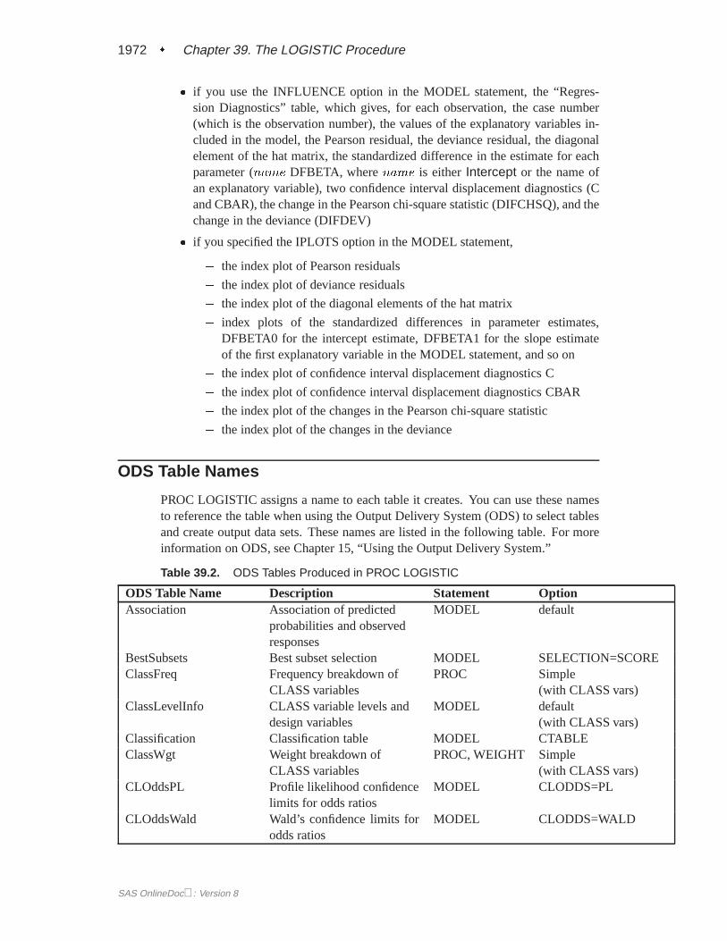
1972 � Chapter 39. The LOGISTIC Procedure
� if you use the INFLUENCE option in the MODEL statement, the “Regres-sion Diagnostics” table, which gives, for each observation, the case number(which is the observation number), the values of the explanatory variables in-cluded in the model, the Pearson residual, the deviance residual, the diagonalelement of the hat matrix, the standardized difference in the estimate for eachparameter (name DFBETA, wherename is eitherIntercept or the name ofan explanatory variable), two confidence interval displacement diagnostics (Cand CBAR), the change in the Pearson chi-square statistic (DIFCHSQ), and thechange in the deviance (DIFDEV)
� if you specified the IPLOTS option in the MODEL statement,
� the index plot of Pearson residuals
� the index plot of deviance residuals
� the index plot of the diagonal elements of the hat matrix
� index plots of the standardized differences in parameter estimates,DFBETA0 for the intercept estimate, DFBETA1 for the slope estimateof the first explanatory variable in the MODEL statement, and so on
� the index plot of confidence interval displacement diagnostics C
� the index plot of confidence interval displacement diagnostics CBAR
� the index plot of the changes in the Pearson chi-square statistic
� the index plot of the changes in the deviance
ODS Table Names
PROC LOGISTIC assigns a name to each table it creates. You can use these namesto reference the table when using the Output Delivery System (ODS) to select tablesand create output data sets. These names are listed in the following table. For moreinformation on ODS, see Chapter 15, “Using the Output Delivery System.”
Table 39.2. ODS Tables Produced in PROC LOGISTIC
ODS Table Name Description Statement OptionAssociation Association of predicted
probabilities and observedresponses
MODEL default
BestSubsets Best subset selection MODEL SELECTION=SCOREClassFreq Frequency breakdown of
CLASS variablesPROC Simple
(with CLASS vars)ClassLevelInfo CLASS variable levels and
design variablesMODEL default
(with CLASS vars)Classification Classification table MODEL CTABLEClassWgt Weight breakdown of
CLASS variablesPROC, WEIGHT Simple
(with CLASS vars)CLOddsPL Profile likelihood confidence
limits for odds ratiosMODEL CLODDS=PL
CLOddsWald Wald’s confidence limits forodds ratios
MODEL CLODDS=WALD
SAS OnlineDoc: Version 8

ODS Table Names � 1973
Table 39.2. (continued)
ODS Table Name Description Statement OptionCLParmPL Profile likelihood confidence
limits for parametersMODEL CLPARM=PL
CLParmWald Wald’s confidence limits forparameters
MODEL CLPARM=WALD
ContrastCoeff L matrix from CONTRAST CONTRAST EContrastEstimate Estimates from CONTRAST CONTRAST ESTIMATE=ContrastTest Wald test for CONTRAST CONTRAST defaultConvergenceStatus Convergence status MODEL defaultCorrB Estimated correlation matrix
of parameter estimatorsMODEL CORRB
CovB Estimated covariance matrixof parameter estimators
MODEL COVB
CumulativeModelTest Test of the cumulative modelassumption
MODEL (ordinal response)
EffectNotInModel Test for effects not in model MODEL SELECTION=S/FFastElimination Fast backward elimination MODEL SELECTION=B,FASTFitStatistics Model fit statistics MODEL defaultGlobalScore Global score test MODEL NOFITGlobalTests Test for global null
hypothesisMODEL default
GoodnessOfFit Pearson and deviancegoodness-of-fit tests
MODEL SCALE
IndexPlots Batch capture of the indexplots
MODEL IPLOTS
Influence Regression diagnostics MODEL INFLUENCEIterHistory Iteration history MODEL ITPRINTLackFitChiSq Hosmer-Lemeshow
chi-square test resultsMODEL LACKFIT
LackFitPartition Partition for the Hosmer-Lemeshow test
MODEL LACKFIT
LastGradient Last evaluation of gradient MODEL ITPRINTLogLikeChange Final change in the log
likelihoodMODEL ITPRINT
ModelBuildingSummary Summary of model building MODEL SELECTION=B/F/SModelInfo Model information PROC defaultOddsRatios Odds ratios MODEL defaultParameterEstimates Maximum likelihood
estimates of modelparameters
MODEL default
RSquare R-square MODEL RSQUAREResidualChiSq Residual chi-square MODEL SELECTION=F/BResponseProfile Response profile PROC defaultSimpleStatistics Summary statistics for
explanatory variablesPROC SIMPLE
TestPrint1 L [cov(b)]L ’ and Lb -c TEST PRINT
SAS OnlineDoc: Version 8

1974 � Chapter 39. The LOGISTIC Procedure
Table 39.2. (continued)
ODS Table Name Description Statement OptionTestPrint2 Ginv(L [cov(b)]L ’) and
Ginv(L [cov(b)]L ’)(Lb -c)TEST PRINT
TestStmts Linear hypotheses testingresults
TEST default
TypeIII Type III tests of effects MODEL default(with CLASS variables)
Examples
Example 39.1. Stepwise Logistic Regression and PredictedValues
Consider a study on cancer remission (Lee 1974). The data, consisting of patientcharacteristics and whether or not cancer remission occurred, are saved in the datasetRemission.
data Remission;input remiss cell smear infil li blast temp;label remiss=’Complete Remission’;datalines;
1 .8 .83 .66 1.9 1.1 .9961 .9 .36 .32 1.4 .74 .9920 .8 .88 .7 .8 .176 .9820 1 .87 .87 .7 1.053 .9861 .9 .75 .68 1.3 .519 .980 1 .65 .65 .6 .519 .9821 .95 .97 .92 1 1.23 .9920 .95 .87 .83 1.9 1.354 1.020 1 .45 .45 .8 .322 .9990 .95 .36 .34 .5 0 1.0380 .85 .39 .33 .7 .279 .9880 .7 .76 .53 1.2 .146 .9820 .8 .46 .37 .4 .38 1.0060 .2 .39 .08 .8 .114 .990 1 .9 .9 1.1 1.037 .991 1 .84 .84 1.9 2.064 1.020 .65 .42 .27 .5 .114 1.0140 1 .75 .75 1 1.322 1.0040 .5 .44 .22 .6 .114 .991 1 .63 .63 1.1 1.072 .9860 1 .33 .33 .4 .176 1.010 .9 .93 .84 .6 1.591 1.021 1 .58 .58 1 .531 1.0020 .95 .32 .3 1.6 .886 .9881 1 .6 .6 1.7 .964 .991 1 .69 .69 .9 .398 .9860 1 .73 .73 .7 .398 .986;
SAS OnlineDoc: Version 8

Example 39.1. Stepwise Logistic Regression and Predicted Values � 1975
The data setRemission contains seven variables. The variableremiss is the cancerremission indicator variable with a value of 1 for remission and a value of 0 fornonremission. The other six variables are the risk factors thought to be related tocancer remission.
The following invocation of PROC LOGISTIC illustrates the use of stepwise selec-tion to identify the prognostic factors for cancer remission. A significance level of0.3 (SLENTRY=0.3) is required to allow a variable into the model, and a signifi-cance level of 0.35 (SLSTAY=0.35) is required for a variable to stay in the model. Adetailed account of the variable selection process is requested by specifying the DE-TAILS option. The Hosmer and Lemeshow goodness-of-fit test for the final selectedmodel is requested by specifying the LACKFIT option. The OUTEST= and COV-OUT options in the PROC LOGISTIC statement create a data set that contains param-eter estimates and their covariances for the final selected model. The DESCENDINGoption causesremiss=1 (remission) to be Ordered Value 1 so that the probability ofremission is modeled. The OUTPUT statement creates a data set that contains thecumulative predicted probabilities and the corresponding confidence limits, and theindividual and cross-validated predicted probabilities for each observation.
title ’Stepwise Regression on Cancer Remission Data’;proc logistic data=Remission descending outest=betas covout;
model remiss=cell smear infil li blast temp/ selection=stepwise
slentry=0.3slstay=0.35detailslackfit;
output out=pred p=phat lower=lcl upper=uclpredprobs=(individual crossvalidate);
run;proc print data=betas;
title2 ’Parameter Estimates and Covariance Matrix’;run;proc print data=pred;
title2 ’Predicted Probabilities and 95% Confidence Limits’;run;
In stepwise selection, an attempt is made to remove any insignificant variables fromthe model before adding a significant variable to the model. Each addition or deletionof a variable to or from a model is listed as a separate step in the displayed output,and at each step a new model is fitted. Details of the model selection steps are shownin Output 39.1.1–Output 39.1.5.
SAS OnlineDoc: Version 8

1976 � Chapter 39. The LOGISTIC Procedure
Output 39.1.1. Startup Model
Stepwise Regression on Cancer Remission Data
The LOGISTIC Procedure
Model Information
Data Set WORK.REMISSIONResponse Variable remiss Complete RemissionNumber of Response Levels 2Number of Observations 27Link Function LogitOptimization Technique Fisher’s scoring
Response Profile
Ordered TotalValue remiss Frequency
1 1 92 0 18
Stepwise Selection Procedure
Step 0. Intercept entered:
Model Convergence Status
Convergence criterion (GCONV=1E-8) satisfied.
Analysis of Maximum Likelihood Estimates
StandardParameter DF Estimate Error Chi-Square Pr > ChiSq
Intercept 1 -0.6931 0.4082 2.8827 0.0895
Residual Chi-Square Test
Chi-Square DF Pr > ChiSq
9.4609 6 0.1493
Analysis of Effects Not in the Model
ScoreEffect DF Chi-Square Pr > ChiSq
cell 1 1.8893 0.1693smear 1 1.0745 0.2999infil 1 1.8817 0.1701li 1 7.9311 0.0049blast 1 3.5258 0.0604temp 1 0.6591 0.4169
SAS OnlineDoc: Version 8

Example 39.1. Stepwise Logistic Regression and Predicted Values � 1977
Output 39.1.2. Step 1 of the Stepwise Analysis
Step 1. Effect li entered:
Model Convergence Status
Convergence criterion (GCONV=1E-8) satisfied.
Model Fit Statistics
InterceptIntercept and
Criterion Only Covariates
AIC 36.372 30.073SC 37.668 32.665-2 Log L 34.372 26.073
Testing Global Null Hypothesis: BETA=0
Test Chi-Square DF Pr > ChiSq
Likelihood Ratio 8.2988 1 0.0040Score 7.9311 1 0.0049Wald 5.9594 1 0.0146
Analysis of Maximum Likelihood Estimates
StandardParameter DF Estimate Error Chi-Square Pr > ChiSq
Intercept 1 -3.7771 1.3786 7.5064 0.0061li 1 2.8973 1.1868 5.9594 0.0146
Association of Predicted Probabilities and Observed Responses
Percent Concordant 84.0 Somers’ D 0.710Percent Discordant 13.0 Gamma 0.732Percent Tied 3.1 Tau-a 0.328Pairs 162 c 0.855
Residual Chi-Square Test
Chi-Square DF Pr > ChiSq
3.1174 5 0.6819
Analysis of Effects Not in the Model
ScoreEffect DF Chi-Square Pr > ChiSq
cell 1 1.1183 0.2903smear 1 0.1369 0.7114infil 1 0.5715 0.4497blast 1 0.0932 0.7601temp 1 1.2591 0.2618
SAS OnlineDoc: Version 8

1978 � Chapter 39. The LOGISTIC Procedure
Output 39.1.3. Step 2 of the Stepwise Analysis
Step 2. Effect temp entered:
Model Convergence Status
Convergence criterion (GCONV=1E-8) satisfied.
Model Fit Statistics
InterceptIntercept and
Criterion Only Covariates
AIC 36.372 30.648SC 37.668 34.535-2 Log L 34.372 24.648
Testing Global Null Hypothesis: BETA=0
Test Chi-Square DF Pr > ChiSq
Likelihood Ratio 9.7239 2 0.0077Score 8.3648 2 0.0153Wald 5.9052 2 0.0522
Analysis of Maximum Likelihood Estimates
StandardParameter DF Estimate Error Chi-Square Pr > ChiSq
Intercept 1 47.8448 46.4381 1.0615 0.3029li 1 3.3017 1.3593 5.9002 0.0151temp 1 -52.4214 47.4897 1.2185 0.2697
Association of Predicted Probabilities and Observed Responses
Percent Concordant 87.0 Somers’ D 0.747Percent Discordant 12.3 Gamma 0.752Percent Tied 0.6 Tau-a 0.345Pairs 162 c 0.873
Residual Chi-Square Test
Chi-Square DF Pr > ChiSq
2.1429 4 0.7095
Analysis of Effects Not in the Model
ScoreEffect DF Chi-Square Pr > ChiSq
cell 1 1.4700 0.2254smear 1 0.1730 0.6775infil 1 0.8274 0.3630blast 1 1.1013 0.2940
SAS OnlineDoc: Version 8

Example 39.1. Stepwise Logistic Regression and Predicted Values � 1979
Output 39.1.4. Step 3 of the Stepwise Analysis
Step 3. Effect cell entered:
Model Convergence Status
Convergence criterion (GCONV=1E-8) satisfied.
Model Fit Statistics
InterceptIntercept and
Criterion Only Covariates
AIC 36.372 29.953SC 37.668 35.137-2 Log L 34.372 21.953
Testing Global Null Hypothesis: BETA=0
Test Chi-Square DF Pr > ChiSq
Likelihood Ratio 12.4184 3 0.0061Score 9.2502 3 0.0261Wald 4.8281 3 0.1848
Analysis of Maximum Likelihood Estimates
StandardParameter DF Estimate Error Chi-Square Pr > ChiSq
Intercept 1 67.6339 56.8875 1.4135 0.2345cell 1 9.6521 7.7511 1.5507 0.2130li 1 3.8671 1.7783 4.7290 0.0297temp 1 -82.0737 61.7124 1.7687 0.1835
Association of Predicted Probabilities and Observed Responses
Percent Concordant 88.9 Somers’ D 0.778Percent Discordant 11.1 Gamma 0.778Percent Tied 0.0 Tau-a 0.359Pairs 162 c 0.889
Residual Chi-Square Test
Chi-Square DF Pr > ChiSq
0.1831 3 0.9803
Analysis of Effects Not in the Model
ScoreEffect DF Chi-Square Pr > ChiSq
smear 1 0.0956 0.7572infil 1 0.0844 0.7714blast 1 0.0208 0.8852
NOTE: No (additional) effects met the 0.3 significance level for entry into themodel.
SAS OnlineDoc: Version 8

1980 � Chapter 39. The LOGISTIC Procedure
Output 39.1.5. Summary of the Stepwise Selection
Summary of Stepwise Selection
Effect Number Score WaldStep Entered Removed DF In Chi-Square Chi-Square Pr > ChiSq
1 li 1 1 7.9311 . 0.00492 temp 1 2 1.2591 . 0.26183 cell 1 3 1.4700 . 0.2254
Prior to the first step, the intercept-only model is fitted and individual score statisticsfor the potential variables are evaluated (Output 39.1.1). In Step 1 (Output 39.1.2),variable li is selected into the model since it is the most significant variable amongthose to be chosen (p = 0:0049 < 0:3). The intermediate model that contains anintercept andli is then fitted.li remains significant (p = 0:0146 < 0:35) and is notremoved. In Step 2 (Output 39.1.3), variabletemp is added to the model. The modelthen contains an intercept and variablesli and temp. Both li and temp remain sig-nificant at 0.035 level; therefore, neitherli nor temp is removed from the model. InStep 4 (Output 39.1.4), variablecell is added to the model. The model then containsan intercept and variablesli, temp, andcell. None of these variables are removedfrom the model since all are significant at the 0.35 level. Finally, none of the remain-ing variables outside the model meet the entry criterion, and the stepwise selection isterminated. A summary of the stepwise selection is displayed in Output 39.1.5.
Output 39.1.6. Display of the LACKFIT Option
Partition for the Hosmer and Lemeshow Test
remiss = 1 remiss = 0Group Total Observed Expected Observed Expected
1 4 0 0.00 4 4.002 3 0 0.03 3 2.973 3 0 0.34 3 2.664 3 1 0.65 2 2.355 3 0 0.84 3 2.166 3 2 1.35 1 1.657 3 2 1.84 1 1.168 3 3 2.15 0 0.859 2 1 1.80 1 0.20
Hosmer and Lemeshow Goodness-of-Fit Test
Chi-Square DF Pr > ChiSq
7.1966 7 0.4087
Results of the Hosmer and Lemeshow test are shown in Output 39.1.6. There is noevidence of a lack of fit in the selected model(p = 0:4087).
SAS OnlineDoc: Version 8

Example 39.1. Stepwise Logistic Regression and Predicted Values � 1981
Output 39.1.7. Data Set of Estimates and Covariances
Stepwise Regression on Cancer Remission DataParameter Estimates and Covariance Matrix
Obs _LINK_ _TYPE_ _STATUS_ _NAME_ Intercept cell
1 LOGIT PARMS 0 Converged ESTIMATE 67.63 9.6522 LOGIT COV 0 Converged Intercept 3236.19 157.0973 LOGIT COV 0 Converged cell 157.10 60.0794 LOGIT COV 0 Converged smear . .5 LOGIT COV 0 Converged infil . .6 LOGIT COV 0 Converged li 64.57 6.9457 LOGIT COV 0 Converged blast . .8 LOGIT COV 0 Converged temp -3483.23 -223.669
Obs smear infil li blast temp _LNLIKE_
1 . . 3.8671 . -82.07 -10.97672 . . 64.5726 . -3483.23 -10.97673 . . 6.9454 . -223.67 -10.97674 . . . . . -10.97675 . . . . . -10.97676 . . 3.1623 . -75.35 -10.97677 . . . . . -10.97678 . . -75.3513 . 3808.42 -10.9767
The data setbetas created by the OUTEST= and COVOUT options is displayed inOutput 39.1.7. The data set contains parameter estimates and the covariance matrixfor the final selected model. Note that all explanatory variables listed in the MODELstatement are included in this data set; however, variables that are not included in thefinal model have all missing values.
SAS OnlineDoc: Version 8

1982 � Chapter 39. The LOGISTIC Procedure
Output 39.1.8. Predicted Probabilities and Confidence Intervals
Stepwise Regression on Cancer Remission DataPredicted Probabilities and 95% Confidence Limits
_r _ _ Le s i b F I Em c m n l t R N I I X X V p
O i e e f a e O T P P P P E h l ub s l a i l s m M O _ _ _ _ L a c cs s l r l i t p _ _ 1 0 1 0 _ t l l
1 1 0.80 0.83 0.66 1.9 1.100 0.996 1 1 0.72265 0.27735 0.56127 0.43873 1 0.72265 0.16892 0.970932 1 0.90 0.36 0.32 1.4 0.740 0.992 1 1 0.57874 0.42126 0.52539 0.47461 1 0.57874 0.26788 0.837623 0 0.80 0.88 0.70 0.8 0.176 0.982 0 0 0.10460 0.89540 0.12940 0.87060 1 0.10460 0.00781 0.634194 0 1.00 0.87 0.87 0.7 1.053 0.986 0 0 0.28258 0.71742 0.32741 0.67259 1 0.28258 0.07498 0.656835 1 0.90 0.75 0.68 1.3 0.519 0.980 1 1 0.71418 0.28582 0.63099 0.36901 1 0.71418 0.25218 0.948766 0 1.00 0.65 0.65 0.6 0.519 0.982 0 0 0.27089 0.72911 0.32731 0.67269 1 0.27089 0.05852 0.689517 1 0.95 0.97 0.92 1.0 1.230 0.992 1 0 0.32156 0.67844 0.27077 0.72923 1 0.32156 0.13255 0.595168 0 0.95 0.87 0.83 1.9 1.354 1.020 0 1 0.60723 0.39277 0.90094 0.09906 1 0.60723 0.10572 0.952879 0 1.00 0.45 0.45 0.8 0.322 0.999 0 0 0.16632 0.83368 0.19136 0.80864 1 0.16632 0.03018 0.56123
10 0 0.95 0.36 0.34 0.5 0.000 1.038 0 0 0.00157 0.99843 0.00160 0.99840 1 0.00157 0.00000 0.6896211 0 0.85 0.39 0.33 0.7 0.279 0.988 0 0 0.07285 0.92715 0.08277 0.91723 1 0.07285 0.00614 0.4998212 0 0.70 0.76 0.53 1.2 0.146 0.982 0 0 0.17286 0.82714 0.36162 0.63838 1 0.17286 0.00637 0.8720613 0 0.80 0.46 0.37 0.4 0.380 1.006 0 0 0.00346 0.99654 0.00356 0.99644 1 0.00346 0.00001 0.4653014 0 0.20 0.39 0.08 0.8 0.114 0.990 0 0 0.00018 0.99982 0.00019 0.99981 1 0.00018 0.00000 0.9648215 0 1.00 0.90 0.90 1.1 1.037 0.990 0 1 0.57122 0.42878 0.64646 0.35354 1 0.57122 0.25303 0.8397316 1 1.00 0.84 0.84 1.9 2.064 1.020 1 1 0.71470 0.28530 0.52787 0.47213 1 0.71470 0.15362 0.9718917 0 0.65 0.42 0.27 0.5 0.114 1.014 0 0 0.00062 0.99938 0.00063 0.99937 1 0.00062 0.00000 0.6266518 0 1.00 0.75 0.75 1.0 1.322 1.004 0 0 0.22289 0.77711 0.26388 0.73612 1 0.22289 0.04483 0.6367019 0 0.50 0.44 0.22 0.6 0.114 0.990 0 0 0.00154 0.99846 0.00158 0.99842 1 0.00154 0.00000 0.7964420 1 1.00 0.63 0.63 1.1 1.072 0.986 1 1 0.64911 0.35089 0.57947 0.42053 1 0.64911 0.26305 0.9055521 0 1.00 0.33 0.33 0.4 0.176 1.010 0 0 0.01693 0.98307 0.01830 0.98170 1 0.01693 0.00029 0.5047522 0 0.90 0.93 0.84 0.6 1.591 1.020 0 0 0.00622 0.99378 0.00652 0.99348 1 0.00622 0.00003 0.5606223 1 1.00 0.58 0.58 1.0 0.531 1.002 1 0 0.25261 0.74739 0.15577 0.84423 1 0.25261 0.06137 0.6359724 0 0.95 0.32 0.30 1.6 0.886 0.988 0 1 0.87011 0.12989 0.96363 0.03637 1 0.87011 0.40910 0.9848125 1 1.00 0.60 0.60 1.7 0.964 0.990 1 1 0.93132 0.06868 0.91983 0.08017 1 0.93132 0.44114 0.9957326 1 1.00 0.69 0.69 0.9 0.398 0.986 1 0 0.46051 0.53949 0.37688 0.62312 1 0.46051 0.16612 0.7852927 0 1.00 0.73 0.73 0.7 0.398 0.986 0 0 0.28258 0.71742 0.32741 0.67259 1 0.28258 0.07498 0.65683
The data setpred created by the OUTPUT statement is displayed in Output 39.1.8. Itcontains all the variables in the input data set, the variablephat for the (cumulative)predicted probability, the variableslcl anducl for the lower and upper confidence lim-its for the probability, and four other variables (viz.,IP–1, IP–0, XP–1, andXP–0)for the PREDPROBS= option. The data set also contains the variable–LEVEL–,indicating the response value to whichphat, lcl, anducl refer. For instance, for thefirst row of the OUTPUT data set, the values of–LEVEL– andphat, lcl, anducl are1, 0.72265, 0.16892 and 0.97093, respectively; this means that the estimated proba-bility that remiss�1 is 0.723 for the given explanatory variable values, and the cor-responding 95% confidence interval is (0.16892, 0.97093). The variablesIP–1 andIP–0 contain the predicted probabilities thatremiss=1 andremiss=0, respectively.Note that values ofphat and IP–1 are identical since they both contain the proba-bilities that remiss=1. The variablesXP–1 andXP–0 contain the cross-validatedpredicted probabilities thatremiss=1 andremiss=0, respectively.
Next, a different variable selection method is used to select prognostic factors forcancer remission, and an efficient algorithm is employed to eliminate insignificantvariables from a model. The following SAS statements invoke PROC LOGISTIC toperform the backward elimination analysis.
SAS OnlineDoc: Version 8

Example 39.1. Stepwise Logistic Regression and Predicted Values � 1983
title ’Backward Elimination on Cancer Remission Data’;proc logistic data=Remission descending;
model remiss=temp cell li smear blast/ selection=backward
fastslstay=0.2ctable;
run;
The backward elimination analysis (SELECTION=BACKWARD) starts with amodel that contains all explanatory variables given in the MODEL statement. Byspecifying the FAST option, PROC LOGISTIC eliminates insignificant variableswithout refitting the model repeatedly. This analysis uses a significance level of 0.2(SLSTAY=0.2) to retain variables in the model, which is different from the previousstepwise analysis where SLSTAY=.35. The CTABLE option is specified to produceclassifications of input observations based on the final selected model.
SAS OnlineDoc: Version 8

1984 � Chapter 39. The LOGISTIC Procedure
Output 39.1.9. Initial Step in Backward Elimination
Backward Elimination on Cancer Remission Data
The LOGISTIC Procedure
Model Information
Data Set WORK.REMISSIONResponse Variable remiss Complete RemissionNumber of Response Levels 2Number of Observations 27Link Function LogitOptimization Technique Fisher’s scoring
Response Profile
Ordered TotalValue remiss Frequency
1 1 92 0 18
Backward Elimination Procedure
Step 0. The following effects were entered:
Intercept temp cell li smear blast
Model Convergence Status
Convergence criterion (GCONV=1E-8) satisfied.
Model Fit Statistics
InterceptIntercept and
Criterion Only Covariates
AIC 36.372 33.857SC 37.668 41.632-2 Log L 34.372 21.857
Testing Global Null Hypothesis: BETA=0
Test Chi-Square DF Pr > ChiSq
Likelihood Ratio 12.5146 5 0.0284Score 9.3295 5 0.0966Wald 4.7284 5 0.4499
SAS OnlineDoc: Version 8
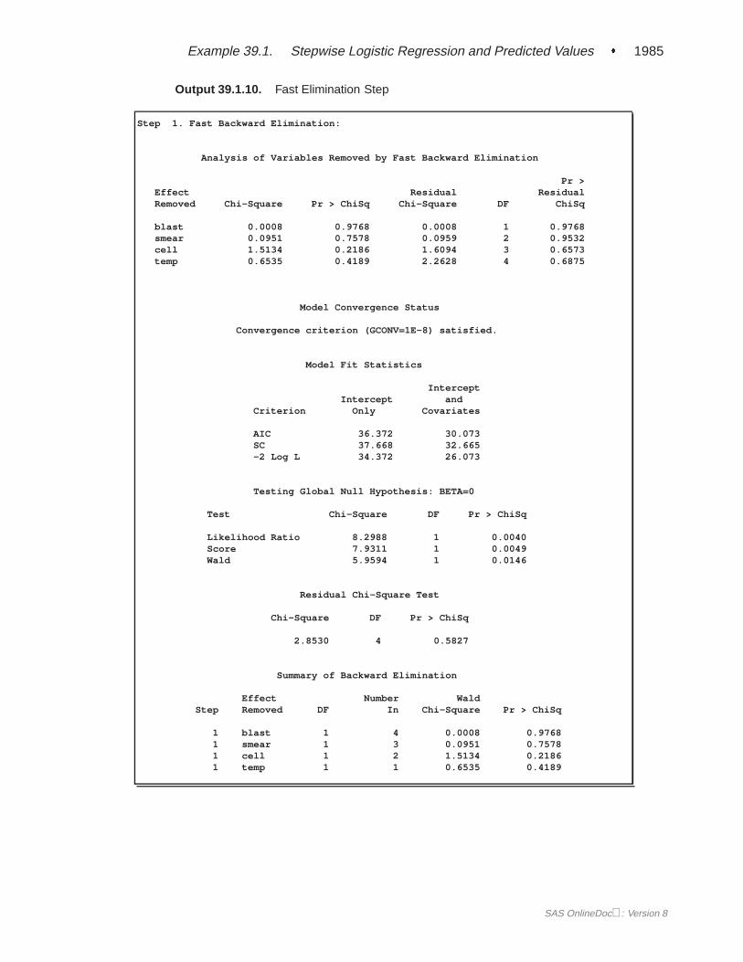
Example 39.1. Stepwise Logistic Regression and Predicted Values � 1985
Output 39.1.10. Fast Elimination Step
Step 1. Fast Backward Elimination:
Analysis of Variables Removed by Fast Backward Elimination
Pr >Effect Residual ResidualRemoved Chi-Square Pr > ChiSq Chi-Square DF ChiSq
blast 0.0008 0.9768 0.0008 1 0.9768smear 0.0951 0.7578 0.0959 2 0.9532cell 1.5134 0.2186 1.6094 3 0.6573temp 0.6535 0.4189 2.2628 4 0.6875
Model Convergence Status
Convergence criterion (GCONV=1E-8) satisfied.
Model Fit Statistics
InterceptIntercept and
Criterion Only Covariates
AIC 36.372 30.073SC 37.668 32.665-2 Log L 34.372 26.073
Testing Global Null Hypothesis: BETA=0
Test Chi-Square DF Pr > ChiSq
Likelihood Ratio 8.2988 1 0.0040Score 7.9311 1 0.0049Wald 5.9594 1 0.0146
Residual Chi-Square Test
Chi-Square DF Pr > ChiSq
2.8530 4 0.5827
Summary of Backward Elimination
Effect Number WaldStep Removed DF In Chi-Square Pr > ChiSq
1 blast 1 4 0.0008 0.97681 smear 1 3 0.0951 0.75781 cell 1 2 1.5134 0.21861 temp 1 1 0.6535 0.4189
SAS OnlineDoc: Version 8

1986 � Chapter 39. The LOGISTIC Procedure
Analysis of Maximum Likelihood Estimates
StandardParameter DF Estimate Error Chi-Square Pr > ChiSq
Intercept 1 -3.7771 1.3786 7.5064 0.0061li 1 2.8973 1.1868 5.9594 0.0146
Association of Predicted Probabilities and Observed Responses
Percent Concordant 84.0 Somers’ D 0.710Percent Discordant 13.0 Gamma 0.732Percent Tied 3.1 Tau-a 0.328Pairs 162 c 0.855
Results of the fast elimination analysis are shown in Output 39.1.9 and Out-put 39.1.10. Initially, a full model containing all six risk factors is fit to the data(Output 39.1.9). In the next step (Output 39.1.10), PROC LOGISTIC removesblast,smear, cell, andtemp from the model all at once. This leavesli and the interceptas the only variables in the final model. Note that in this analysis, only parameterestimates for the final model are displayed because the DETAILS option has not beenspecified.
Note that you can also use the FAST option when SELECTION=STEPWISE. How-ever, the FAST option operates only on backward elimination steps. In this example,the stepwise process only adds variables, so the FAST option would not be useful.
SAS OnlineDoc: Version 8

Example 39.1. Stepwise Logistic Regression and Predicted Values � 1987
Output 39.1.11. Classifying Input Observations
Classification Table
Correct Incorrect PercentagesProb Non- Non- Sensi- Speci- False False
Level Event Event Event Event Correct tivity ficity POS NEG
0.060 9 0 18 0 33.3 100.0 0.0 66.7 .0.080 9 2 16 0 40.7 100.0 11.1 64.0 0.00.100 9 4 14 0 48.1 100.0 22.2 60.9 0.00.120 9 4 14 0 48.1 100.0 22.2 60.9 0.00.140 9 7 11 0 59.3 100.0 38.9 55.0 0.00.160 9 10 8 0 70.4 100.0 55.6 47.1 0.00.180 9 10 8 0 70.4 100.0 55.6 47.1 0.00.200 8 13 5 1 77.8 88.9 72.2 38.5 7.10.220 8 13 5 1 77.8 88.9 72.2 38.5 7.10.240 8 13 5 1 77.8 88.9 72.2 38.5 7.10.260 6 13 5 3 70.4 66.7 72.2 45.5 18.80.280 6 13 5 3 70.4 66.7 72.2 45.5 18.80.300 6 13 5 3 70.4 66.7 72.2 45.5 18.80.320 6 14 4 3 74.1 66.7 77.8 40.0 17.60.340 5 14 4 4 70.4 55.6 77.8 44.4 22.20.360 5 14 4 4 70.4 55.6 77.8 44.4 22.20.380 5 15 3 4 74.1 55.6 83.3 37.5 21.10.400 5 15 3 4 74.1 55.6 83.3 37.5 21.10.420 5 15 3 4 74.1 55.6 83.3 37.5 21.10.440 5 15 3 4 74.1 55.6 83.3 37.5 21.10.460 4 16 2 5 74.1 44.4 88.9 33.3 23.80.480 4 16 2 5 74.1 44.4 88.9 33.3 23.80.500 4 16 2 5 74.1 44.4 88.9 33.3 23.80.520 4 16 2 5 74.1 44.4 88.9 33.3 23.80.540 3 16 2 6 70.4 33.3 88.9 40.0 27.30.560 3 16 2 6 70.4 33.3 88.9 40.0 27.30.580 3 16 2 6 70.4 33.3 88.9 40.0 27.30.600 3 16 2 6 70.4 33.3 88.9 40.0 27.30.620 3 16 2 6 70.4 33.3 88.9 40.0 27.30.640 3 16 2 6 70.4 33.3 88.9 40.0 27.30.660 3 16 2 6 70.4 33.3 88.9 40.0 27.30.680 3 16 2 6 70.4 33.3 88.9 40.0 27.30.700 3 16 2 6 70.4 33.3 88.9 40.0 27.30.720 2 16 2 7 66.7 22.2 88.9 50.0 30.40.740 2 16 2 7 66.7 22.2 88.9 50.0 30.40.760 2 16 2 7 66.7 22.2 88.9 50.0 30.40.780 2 16 2 7 66.7 22.2 88.9 50.0 30.40.800 2 17 1 7 70.4 22.2 94.4 33.3 29.20.820 2 17 1 7 70.4 22.2 94.4 33.3 29.20.840 0 17 1 9 63.0 0.0 94.4 100.0 34.60.860 0 17 1 9 63.0 0.0 94.4 100.0 34.60.880 0 17 1 9 63.0 0.0 94.4 100.0 34.60.900 0 17 1 9 63.0 0.0 94.4 100.0 34.60.920 0 17 1 9 63.0 0.0 94.4 100.0 34.60.940 0 17 1 9 63.0 0.0 94.4 100.0 34.60.960 0 18 0 9 66.7 0.0 100.0 . 33.3
Results of the CTABLE option are shown in Output 39.1.11. Each row of the “Classi-fication Table” corresponds to a cutpoint applied to the predicted probabilities, whichis given in the Prob Level column. The2 � 2 frequency tables of observed and pre-dicted responses are given by the next four columns. For example, with a cutpoint of0.5, 4 events and 16 nonevents were classified correctly. On the other hand, 2 non-events were incorrectly classified as events and 5 events were incorrectly classified asnonevents. For this cutpoint, the correct classification rate is 20/27 (=74.1%), whichis given in the sixth column. Accuracy of the classification is summarized by the
SAS OnlineDoc: Version 8

1988 � Chapter 39. The LOGISTIC Procedure
sensitivity, specificity, and false positive and negative rates, which are displayed inthe last four columns. You can control the number of cutpoints used, and their values,by using the PPROB= option.
Example 39.2. Ordinal Logistic Regression
Consider a study of the effects on taste of various cheese additives. Researcherstested four cheese additives and obtained 52 response ratings for each additive. Eachresponse was measured on a scale of nine categories ranging from strong dislike (1)to excellent taste (9). The data, given in McCullagh and Nelder (1989, p. 175) inthe form of a two-way frequency table of additive by rating, are saved in the data setCheese.
data Cheese;do Additive = 1 to 4;
do y = 1 to 9;input freq @@;output;
end;end;label y=’Taste Rating’;datalines;
0 0 1 7 8 8 19 8 16 9 12 11 7 6 1 0 01 1 6 8 23 7 5 1 00 0 0 1 3 7 14 16 11;
The data setCheese contains the variablesy, Additive, and freq. The variableycontains the response rating. The variableAdditive specifies the cheese additive (1,2, 3, or 4). The variablefreq gives the frequency with which each additive receivedeach rating.
The response variabley is ordinally scaled. A cumulative logit model is used toinvestigate the effects of the cheese additives on taste. The following SAS statementsinvoke PROC LOGISTIC to fit this model withy as the response variable and threeindicator variables as explanatory variables, with the fourth additive as the referencelevel. With this parameterization, eachAdditive parameter compares an additive tothe fourth additive. The COVB option produces the estimated covariance matrix.
proc logistic data=Cheese;freq freq;class Additive (param=ref ref=’4’);model y=Additive / covb;title1 ’Multiple Response Cheese Tasting Experiment’;
run;
Results of the analysis are shown in Output 39.2.1, and the estimated covariancematrix is displayed in Output 39.2.2.
SAS OnlineDoc: Version 8

Example 39.2. Ordinal Logistic Regression � 1989
Since the strong dislike (y=1) end of the rating scale is associated with lower Or-dered Values in the Response Profile table, the probability of disliking the additivesis modeled.
The score chi-square for testing the proportional odds assumption is 17.287, whichis not significant with respect to a chi-square distribution with 21 degrees of free-dom(p = 0:694). This indicates that the proportional odds model adequately fits thedata. The positive value (1.6128) for the parameter estimate forAdditive1 indicatesa tendency towards the lower-numbered categories of the first cheese additive rela-tive to the fourth. In other words, the fourth additive is better in taste than the firstadditive. Each of the second and the third additives is less favorable than the fourthadditive. The relative magnitudes of these slope estimates imply the preference or-dering: fourth, first, third, second.
SAS OnlineDoc: Version 8

1990 � Chapter 39. The LOGISTIC Procedure
Output 39.2.1. Proportional Odds Model Regression Analysis
Multiple Response Cheese Tasting Experiment
The LOGISTIC Procedure
Model Information
Data Set WORK.CHEESEResponse Variable y Taste RatingNumber of Response Levels 9Number of Observations 28Frequency Variable freqSum of Frequencies 208Link Function LogitOptimization Technique Fisher’s scoring
Response Profile
Ordered TotalValue y Frequency
1 1 72 2 103 3 194 4 275 5 416 6 287 7 398 8 259 9 12
NOTE: 8 observations having zero frequencies or weights were excluded sincethey do not contribute to the analysis.
Model Convergence Status
Convergence criterion (GCONV=1E-8) satisfied.
Score Test for the Proportional Odds Assumption
Chi-Square DF Pr > ChiSq
17.2866 21 0.6936
Model Fit Statistics
InterceptIntercept and
Criterion Only Covariates
AIC 875.802 733.348SC 902.502 770.061-2 Log L 859.802 711.348
Testing Global Null Hypothesis: BETA=0
Test Chi-Square DF Pr > ChiSq
Likelihood Ratio 148.4539 3 <.0001Score 111.2670 3 <.0001Wald 115.1504 3 <.0001
SAS OnlineDoc: Version 8

Example 39.2. Ordinal Logistic Regression � 1991
Analysis of Maximum Likelihood Estimates
StandardParameter DF Estimate Error Chi-Square Pr > ChiSq
Intercept 1 -7.0801 0.5624 158.4851 <.0001Intercept2 1 -6.0249 0.4755 160.5500 <.0001Intercept3 1 -4.9254 0.4272 132.9484 <.0001Intercept4 1 -3.8568 0.3902 97.7087 <.0001Intercept5 1 -2.5205 0.3431 53.9704 <.0001Intercept6 1 -1.5685 0.3086 25.8374 <.0001Intercept7 1 -0.0669 0.2658 0.0633 0.8013Intercept8 1 1.4930 0.3310 20.3439 <.0001Additive 1 1 1.6128 0.3778 18.2265 <.0001Additive 2 1 4.9645 0.4741 109.6427 <.0001Additive 3 1 3.3227 0.4251 61.0931 <.0001
Association of Predicted Probabilities and Observed Responses
Percent Concordant 67.6 Somers’ D 0.578Percent Discordant 9.8 Gamma 0.746Percent Tied 22.6 Tau-a 0.500Pairs 18635 c 0.789
Output 39.2.2. Estimated Covariance Matrix
Multiple Response Cheese Tasting Experiment
The LOGISTIC Procedure
Estimated Covariance Matrix
Variable Intercept Intercept2 Intercept3 Intercept4 Intercept5
Intercept 0.316291 0.219581 0.176278 0.147694 0.114024Intercept2 0.219581 0.226095 0.177806 0.147933 0.11403Intercept3 0.176278 0.177806 0.182473 0.148844 0.114092Intercept4 0.147694 0.147933 0.148844 0.152235 0.114512Intercept5 0.114024 0.11403 0.114092 0.114512 0.117713Intercept6 0.091085 0.091081 0.091074 0.091109 0.091821Intercept7 0.057814 0.057813 0.057807 0.05778 0.057721Intercept8 0.041304 0.041304 0.0413 0.041277 0.041162Additive1 -0.09419 -0.09421 -0.09427 -0.09428 -0.09246Additive2 -0.18686 -0.18161 -0.1687 -0.14717 -0.11415Additive3 -0.13565 -0.13569 -0.1352 -0.13118 -0.11207
Estimated Covariance Matrix
Variable Intercept6 Intercept7 Intercept8 Additive1 Additive2 Additive3
Intercept 0.091085 0.057814 0.041304 -0.09419 -0.18686 -0.13565Intercept2 0.091081 0.057813 0.041304 -0.09421 -0.18161 -0.13569Intercept3 0.091074 0.057807 0.0413 -0.09427 -0.1687 -0.1352Intercept4 0.091109 0.05778 0.041277 -0.09428 -0.14717 -0.13118Intercept5 0.091821 0.057721 0.041162 -0.09246 -0.11415 -0.11207Intercept6 0.09522 0.058312 0.041324 -0.08521 -0.09113 -0.09122Intercept7 0.058312 0.07064 0.04878 -0.06041 -0.05781 -0.05802Intercept8 0.041324 0.04878 0.109562 -0.04436 -0.0413 -0.04143Additive1 -0.08521 -0.06041 -0.04436 0.142715 0.094072 0.092128Additive2 -0.09113 -0.05781 -0.0413 0.094072 0.22479 0.132877Additive3 -0.09122 -0.05802 -0.04143 0.092128 0.132877 0.180709
SAS OnlineDoc: Version 8
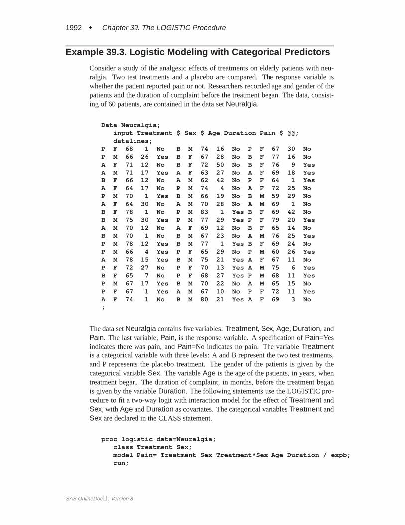
1992 � Chapter 39. The LOGISTIC Procedure
Example 39.3. Logistic Modeling with Categorical Predictors
Consider a study of the analgesic effects of treatments on elderly patients with neu-ralgia. Two test treatments and a placebo are compared. The response variable iswhether the patient reported pain or not. Researchers recorded age and gender of thepatients and the duration of complaint before the treatment began. The data, consist-ing of 60 patients, are contained in the data setNeuralgia.
Data Neuralgia;input Treatment $ Sex $ Age Duration Pain $ @@;datalines;
P F 68 1 No B M 74 16 No P F 67 30 NoP M 66 26 Yes B F 67 28 No B F 77 16 NoA F 71 12 No B F 72 50 No B F 76 9 YesA M 71 17 Yes A F 63 27 No A F 69 18 YesB F 66 12 No A M 62 42 No P F 64 1 YesA F 64 17 No P M 74 4 No A F 72 25 NoP M 70 1 Yes B M 66 19 No B M 59 29 NoA F 64 30 No A M 70 28 No A M 69 1 NoB F 78 1 No P M 83 1 Yes B F 69 42 NoB M 75 30 Yes P M 77 29 Yes P F 79 20 YesA M 70 12 No A F 69 12 No B F 65 14 NoB M 70 1 No B M 67 23 No A M 76 25 YesP M 78 12 Yes B M 77 1 Yes B F 69 24 NoP M 66 4 Yes P F 65 29 No P M 60 26 YesA M 78 15 Yes B M 75 21 Yes A F 67 11 NoP F 72 27 No P F 70 13 Yes A M 75 6 YesB F 65 7 No P F 68 27 Yes P M 68 11 YesP M 67 17 Yes B M 70 22 No A M 65 15 NoP F 67 1 Yes A M 67 10 No P F 72 11 YesA F 74 1 No B M 80 21 Yes A F 69 3 No;
The data setNeuralgia contains five variables:Treatment, Sex, Age, Duration, andPain. The last variable,Pain, is the response variable. A specification ofPain=Yesindicates there was pain, andPain=No indicates no pain. The variableTreatmentis a categorical variable with three levels: A and B represent the two test treatments,and P represents the placebo treatment. The gender of the patients is given by thecategorical variableSex. The variableAge is the age of the patients, in years, whentreatment began. The duration of complaint, in months, before the treatment beganis given by the variableDuration. The following statements use the LOGISTIC pro-cedure to fit a two-way logit with interaction model for the effect ofTreatment andSex, with Age andDuration as covariates. The categorical variablesTreatment andSex are declared in the CLASS statement.
proc logistic data=Neuralgia;class Treatment Sex;model Pain= Treatment Sex Treatment*Sex Age Duration / expb;run;
SAS OnlineDoc: Version 8

Example 39.3. Logistic Modeling with Categorical Predictors � 1993
In this analysis, PROC LOGISTIC models the probability of no pain (Pain=No).By default, effect coding is used to represent the CLASS variables. Two dummyvariables are created forTreatment and one forSex, as shown in Output 39.3.1.
Output 39.3.1. Effect Coding of CLASS Variables
The LOGISTIC Procedure
Class Level Information
DesignVariables
Class Value 1 2
Treatment A 1 0B 0 1P -1 -1
Sex F 1M -1
PROC LOGISTIC displays a table of the Type III analysis of effects based on theWald test (Output 39.3.2). Note that theTreatment*Sex interaction and the durationof complaint are not statistically significant (p =0.9318 andp =0.8752, respectively).This indicates that there is no evidence that the treatments affect pain differently inmen and women, and no evidence that the pain outcome is related to the duration ofpain.
Output 39.3.2. Wald Tests of Individual Effects
The LOGISTIC Procedure
Type III Analysis of Effects
WaldEffect DF Chi-Square Pr > ChiSq
Treatment 2 11.9886 0.0025Sex 1 5.3104 0.0212Treatment*Sex 2 0.1412 0.9318Age 1 7.2744 0.0070Duration 1 0.0247 0.8752
Parameter estimates are displayed in Output 39.3.3. The Exp(Est) column containsthe exponentiated parameter estimates. These values may, but do not necessarily,represent odds ratios for the corresponding variables. For continuous explanatoryvariables, the Exp(Est) value corresponds to the odds ratio for a unit increase of thecorresponding variable. For CLASS variables using the effect coding, the Exp(Est)values have no direct interpretation as a comparison of levels. However, when thereference coding is used, the Exp(Est) values represent the odds ratio between thecorresponding level and the last level. Following the parameter estimates table, PROCLOGISTIC displays the odds ratio estimates for those variables that are not involvedin any interaction terms. If the variable is a CLASS variable, the odds ratio estimatecomparing each level with the last level is computed regardless of the coding scheme.In this analysis, since the model contains theTreatment*Sex interaction term, the
SAS OnlineDoc: Version 8

1994 � Chapter 39. The LOGISTIC Procedure
odds ratios forTreatment and Sex were not computed. The odds ratio estimatesfor Age andDuration are precisely the values given in the Exp(Est) column in theparameter estimates table.
Output 39.3.3. Parameter Estimates with Effect Coding
The LOGISTIC Procedure
Analysis of Maximum Likelihood Estimates
StandardParameter DF Estimate Error Chi-Square Pr > ChiSq Exp(Est)
Intercept 1 19.2236 7.1315 7.2661 0.0070 2.232E8Treatment A 1 0.8483 0.5502 2.3773 0.1231 2.336Treatment B 1 1.4949 0.6622 5.0956 0.0240 4.459Sex F 1 0.9173 0.3981 5.3104 0.0212 2.503Treatment*Sex A F 1 -0.2010 0.5568 0.1304 0.7180 0.818Treatment*Sex B F 1 0.0487 0.5563 0.0077 0.9302 1.050Age 1 -0.2688 0.0996 7.2744 0.0070 0.764Duration 1 0.00523 0.0333 0.0247 0.8752 1.005
Odds Ratio Estimates
Point 95% WaldEffect Estimate Confidence Limits
Age 0.764 0.629 0.929Duration 1.005 0.942 1.073
The following PROC LOGISTIC statements illustrate the use of forward selectionon the data setNeuralgia to identify the effects that differentiate the twoPain re-sponses. The option SELECTION=FORWARD is specified to carry out the forwardselection. Although it is the default, the option RULE=SINGLE is explicitly specifiedto select one effect in each step where the selection must maintain model hierarchy.The termTreatment|Sex@2 illustrates another way to specify main effects and two-way interaction as is available in other procedures such as PROC GLM. (Note that,in this case, the “@2” is unnecessary because no interactions besides the two-wayinteraction are possible).
proc logistic data=Neuralgia;class Treatment Sex;model Pain=Treatment|Sex@2 Age Duration/selection=forward
rule=singleexpb;
run;
Results of the forward selection process are summarized in Output 39.3.4. The vari-able Treatment is selected first, followed byAge and thenSex. The results areconsistent with the previous analysis (Output 39.3.2) in which theTreatment*Sexinteraction andDuration are not statistically significant.
SAS OnlineDoc: Version 8

Example 39.3. Logistic Modeling with Categorical Predictors � 1995
Output 39.3.4. Effects Selected into the Model
Summary of Forward Selection
Effect Number ScoreStep Entered DF In Chi-Square Pr > ChiSq
1 Treatment 2 1 13.7143 0.00112 Age 1 2 10.6038 0.00113 Sex 1 3 5.9959 0.0143
Output 39.3.5 shows the Type III analysis of effects, the parameter estimates, and theodds ratio estimates for the selected model. All three variables,Treatment, Age,andSex, are statistically significant at the 0.05 level (p =0.0011,p =0.0011, andp =0.0143, respectively). Since the selected model does not contain theTreat-ment*Sex interaction, odds ratios forTreatment andSex are computed. The es-timated odds ratio is 24.022 for treatment A versus placebo, 41.528 for Treatment Bversus placebo, and 6.194 for female patients versus male patients. Note that theseodds ratio estimates are not the same as the corresponding values in the Exp(Est)column in the parameter estimates table because effect coding was used. From Out-put 39.3.5, it is evident that both Treatment A and Treatment B are better than theplacebo in reducing pain; females tend to have better improvement than males; andyounger patients are faring better than older patients.
Output 39.3.5. Type III Effects and Parameter Estimates with Effect Coding
Type III Analysis of Effects
WaldEffect DF Chi-Square Pr > ChiSq
Treatment 2 12.6928 0.0018Sex 1 5.3013 0.0213Age 1 7.6314 0.0057
Analysis of Maximum Likelihood Estimates
StandardParameter DF Estimate Error Chi-Square Pr > ChiSq Exp(Est)
Intercept 1 19.0804 6.7882 7.9007 0.0049 1.9343E8Treatment A 1 0.8772 0.5274 2.7662 0.0963 2.404Treatment B 1 1.4246 0.6036 5.5711 0.0183 4.156Sex F 1 0.9118 0.3960 5.3013 0.0213 2.489Age 1 -0.2650 0.0959 7.6314 0.0057 0.767
Odds Ratio Estimates
Point 95% WaldEffect Estimate Confidence Limits
Treatment A vs P 24.022 3.295 175.121Treatment B vs P 41.528 4.500 383.262Sex F vs M 6.194 1.312 29.248Age 0.767 0.636 0.926
SAS OnlineDoc: Version 8

1996 � Chapter 39. The LOGISTIC Procedure
Finally, PROC LOGISTIC is invoked to refit the previously selected model usingreference coding for the CLASS variables. Two CONTRAST statments are specified.The one labeled ’Pairwise’ specifies three rows in the contrast matrix, L, for all thepairwise comparisons between the three levels ofTreatment. The contrast labeled’Female vs Male’ compares female to male patients. The option ESTIMATE=EXPis specified in both CONTRAST statements to exponentiate the estimates ofL0�.With the given specification of contrast coefficients, the first row of the ’Pairwise’CONTRAST statement corresponds to the odds ratio of A versus P, the second rowcorresponds to B versus P, and the third row corresponds to A versus B. There is onlyone row in the ’Female vs Male’ CONTRAST statement, and it corresponds to theodds ratio comparing female to male patients.
proc logistic data=Neuralgia;class Treatment Sex /param=ref;model Pain= Treatment Sex age;contrast ’Pairwise’ Treatment 1 0 -1,
Treatment 0 1 -1,Treatment 1 -1 0 / estimate=exp;
contrast ’Female vs Male’ Sex 1 -1 / estimate=exp;run;
Output 39.3.6. Reference Coding of CLASS Variables
The LOGISTIC Procedure
Class Level Information
DesignVariables
Class Value 1 2
Treatment A 1 0B 0 1P 0 0
Sex F 1M 0
The reference coding is shown in Output 39.3.6. The Type III analysis of effects,the parameter estimates for the reference coding, and the odds ratio estimates aredisplayed in Output 39.3.7. Although the parameter estimates are different (becauseof the different parameterizations), the “Type III Analysis of Effects” table and the“Odds Ratio” table remain the same as in Output 39.3.5. With effect coding, thetreatment A parameter estimate (0.8772) estimates the effect of treatment A comparedto the average effect of treatments A, B, and placebo. The treatment A estimate(3.1790) under the reference coding estimates the difference in effect of treatment Aand the placebo treatment.
SAS OnlineDoc: Version 8

Example 39.4. Logistic Modeling with Categorical Predictors � 1997
Output 39.3.7. Type III Effects and Parameter Estimates with Reference Coding
The LOGISTIC Procedure
Type III Analysis of Effects
WaldEffect DF Chi-Square Pr > ChiSq
Treatment 2 12.6928 0.0018Sex 1 5.3013 0.0213Age 1 7.6314 0.0057
Analysis of Maximum Likelihood Estimates
StandardParameter DF Estimate Error Chi-Square Pr > ChiSq
Intercept 1 15.8669 6.4056 6.1357 0.0132Treatment A 1 3.1790 1.0135 9.8375 0.0017Treatment B 1 3.7264 1.1339 10.8006 0.0010Sex F 1 1.8235 0.7920 5.3013 0.0213Age 1 -0.2650 0.0959 7.6314 0.0057
Odds Ratio Estimates
Point 95% WaldEffect Estimate Confidence Limits
Treatment A vs P 24.022 3.295 175.121Treatment B vs P 41.528 4.500 383.262Sex F vs M 6.194 1.312 29.248Age 0.767 0.636 0.926
Output 39.3.8 contains two tables: the “Contrast Test Results” table and the “ContrastRows Estimation and Testing Results” table. The former contains the overall Waldtest for each CONTRAST statement. Although three rows are specifed in the ’Pair-wise’ CONTRAST statement, there are only two degrees of freedom, and the Waldtest result is identical to the Type III analysis ofTreatment in Output 39.3.7. Thelatter table contains estimates and tests of individual contrast rows. The estimatesfor the first two rows of the ’Pairwise’ CONTRAST statement are the same as thosegiven in the “Odds Ratio Estimates” table (in Output 39.3.7). Both treatments A andB are highly effective over placebo in reducing pain. The third row estimates the oddsratio comparing A to B. The 95% confidence interval for this odds ratio is (0.0932,3.5889), indicating that the pain reduction effects of these two test treatments are notthat different. Again, the ’Female vs Male’ contrast shows that female patients faredbetter in obtaining relief from pain than male patients.
SAS OnlineDoc: Version 8

1998 � Chapter 39. The LOGISTIC Procedure
Output 39.3.8. Results of CONTRAST Statements
The LOGISTIC Procedure
Contrast Test Results
WaldContrast DF Chi-Square Pr > ChiSq
Pairwise 2 12.6928 0.0018Female vs Male 1 5.3013 0.0213
Contrast Rows Estimation and Testing Results
Standard Lower UpperContrast Type Row Estimate Error Alpha Limit Limit
Pairwise EXP 1 24.0218 24.3473 0.05 3.2951 175.1Pairwise EXP 2 41.5284 47.0877 0.05 4.4998 383.3Pairwise EXP 3 0.5784 0.5387 0.05 0.0932 3.5889Female vs Male EXP 1 6.1937 4.9053 0.05 1.3116 29.2476
Contrast Rows Estimation and Testing Results
WaldContrast Type Row Chi-Square Pr > ChiSq
Pairwise EXP 1 9.8375 0.0017Pairwise EXP 2 10.8006 0.0010Pairwise EXP 3 0.3455 0.5567Female vs Male EXP 1 5.3013 0.0213
Example 39.4. Logistic Regression Diagnostics
In a controlled experiment to study the effect of the rate and volume of air inspiredon a transient reflex vaso-constriction in the skin of the digits, 39 tests under variouscombinations of rate and volume of air inspired were obtained (Finney 1947). Theend point of each test is whether or not vaso-constriction occurred. Pregibon (1981)uses this set of data to illustrate the diagnostic measures he proposes for detecting in-fluential observations and to quantify their effects on various aspects of the maximumlikelihood fit.
The vaso-constriction data are saved in the data setvaso:
data vaso;length Response $12;input Volume Rate Response @@;LogVolume=log(Volume);LogRate=log(Rate);datalines;
3.70 0.825 constrict 3.50 1.09 constrict1.25 2.50 constrict 0.75 1.50 constrict0.80 3.20 constrict 0.70 3.50 constrict0.60 0.75 no_constrict 1.10 1.70 no_constrict0.90 0.75 no_constrict 0.90 0.45 no_constrict0.80 0.57 no_constrict 0.55 2.75 no_constrict0.60 3.00 no_constrict 1.40 2.33 constrict
SAS OnlineDoc: Version 8

Example 39.4. Logistic Regression Diagnostics � 1999
0.75 3.75 constrict 2.30 1.64 constrict3.20 1.60 constrict 0.85 1.415 constrict1.70 1.06 no_constrict 1.80 1.80 constrict0.40 2.00 no_constrict 0.95 1.36 no_constrict1.35 1.35 no_constrict 1.50 1.36 no_constrict1.60 1.78 constrict 0.60 1.50 no_constrict1.80 1.50 constrict 0.95 1.90 no_constrict1.90 0.95 constrict 1.60 0.40 no_constrict2.70 0.75 constrict 2.35 0.03 no_constrict1.10 1.83 no_constrict 1.10 2.20 constrict1.20 2.00 constrict 0.80 3.33 constrict0.95 1.90 no_constrict 0.75 1.90 no_constrict1.30 1.625 constrict;
In the data setvaso, the variableResponse represents the outcome of a test. ThevariableLogVolume represents the log of the volume of air intake, and the variableLogRate represents the log of the rate of air intake.
The following SAS statements invoke PROC LOGISTIC to fit a logistic regressionmodel to the vaso-constriction data, whereResponse is the response variable, andLogRate andLogVolume are the explanatory variables. The INFLUENCE optionand the IPLOTS option are specified to display the regression diagnostics and theindex plots.
title ’Occurrence of Vaso-Constriction’;proc logistic data=vaso;
model Response=LogRate LogVolume/influence iplots;run;
Results of the model fit are shown in Output 39.4.1. BothLogRate andLogVolumeare statistically significant to the occurrence of vaso-constriction (p = 0:0131 andp = 0:0055, respectively). Their positive parameter estimates indicate that a higherinspiration rate or a larger volume of air intake is likely to increase the probability ofvaso-constriction.
SAS OnlineDoc: Version 8

2000 � Chapter 39. The LOGISTIC Procedure
Output 39.4.1. Logistic Regression Analysis for Vaso-Constriction Data
Occurrence of Vaso-Constriction
The LOGISTIC Procedure
Model Information
Data Set WORK.VASOResponse Variable ResponseNumber of Response Levels 2Number of Observations 39Link Function LogitOptimization Technique Fisher’s scoring
Response Profile
Ordered TotalValue Response Frequency
1 constrict 202 no_constrict 19
Model Convergence Status
Convergence criterion (GCONV=1E-8) satisfied.
Model Fit Statistics
InterceptIntercept and
Criterion Only Covariates
AIC 56.040 35.227SC 57.703 40.218-2 Log L 54.040 29.227
Testing Global Null Hypothesis: BETA=0
Test Chi-Square DF Pr > ChiSq
Likelihood Ratio 24.8125 2 <.0001Score 16.6324 2 0.0002Wald 7.8876 2 0.0194
Analysis of Maximum Likelihood Estimates
StandardParameter DF Estimate Error Chi-Square Pr > ChiSq
Intercept 1 -2.8754 1.3208 4.7395 0.0295LogRate 1 4.5617 1.8380 6.1597 0.0131LogVolume 1 5.1793 1.8648 7.7136 0.0055
Association of Predicted Probabilities and Observed Responses
Percent Concordant 93.7 Somers’ D 0.874Percent Discordant 6.3 Gamma 0.874Percent Tied 0.0 Tau-a 0.448Pairs 380 c 0.937
SAS OnlineDoc: Version 8
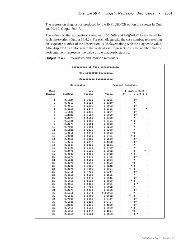
Example 39.4. Logistic Regression Diagnostics � 2001
The regression diagnostics produced by the INFLUENCE option are shown in Out-put 39.4.2–Output 39.4.7.
The values of the explanatory variables (LogRate and LogVolume) are listed foreach observation (Output 39.4.2). For each diagnostic, the case number, representingthe sequence number of the observation, is displayed along with the diagnostic value.Also displayed is a plot where the vertical axis represents the case number and thehorizontal axis represents the value of the diagnostic statistic.
Output 39.4.2. Covariates and Pearson Residuals
Occurrence of Vaso-Constriction
The LOGISTIC Procedure
Regression Diagnostics
Covariates Pearson Residual
Case Log (1 unit = 0.44)Number LogRate Volume Value -8 -4 0 2 4 6 8
1 -0.1924 1.3083 0.2205 | |* |2 0.0862 1.2528 0.1349 | * |3 0.9163 0.2231 0.2923 | |* |4 0.4055 -0.2877 3.5181 | | *|5 1.1632 -0.2231 0.5287 | |* |6 1.2528 -0.3567 0.6090 | |* |7 -0.2877 -0.5108 -0.0328 | * |8 0.5306 0.0953 -1.0196 | * | |9 -0.2877 -0.1054 -0.0938 | * |
10 -0.7985 -0.1054 -0.0293 | * |11 -0.5621 -0.2231 -0.0370 | * |12 1.0116 -0.5978 -0.5073 | *| |13 1.0986 -0.5108 -0.7751 | * | |14 0.8459 0.3365 0.2559 | |* |15 1.3218 -0.2877 0.4352 | |* |16 0.4947 0.8329 0.1576 | * |17 0.4700 1.1632 0.0709 | * |18 0.3471 -0.1625 2.9062 | | * |19 0.0583 0.5306 -1.0718 | * | |20 0.5878 0.5878 0.2405 | |* |21 0.6931 -0.9163 -0.1076 | * |22 0.3075 -0.0513 -0.4193 | *| |23 0.3001 0.3001 -1.0242 | * | |24 0.3075 0.4055 -1.3684 | * | |25 0.5766 0.4700 0.3347 | |* |26 0.4055 -0.5108 -0.1595 | * |27 0.4055 0.5878 0.3645 | |* |28 0.6419 -0.0513 -0.8989 | * | |29 -0.0513 0.6419 0.8981 | | * |30 -0.9163 0.4700 -0.0992 | * |31 -0.2877 0.9933 0.6198 | |* |32 -3.5066 0.8544 -0.00073 | * |33 0.6043 0.0953 -1.2062 | * | |34 0.7885 0.0953 0.5447 | |* |35 0.6931 0.1823 0.5404 | |* |36 1.2030 -0.2231 0.4828 | |* |37 0.6419 -0.0513 -0.8989 | * | |38 0.6419 -0.2877 -0.4874 | *| |39 0.4855 0.2624 0.7053 | | * |
SAS OnlineDoc: Version 8

2002 � Chapter 39. The LOGISTIC Procedure
Output 39.4.3. Deviance Residuals and Hat Matrix Diagonal Elements
Regression Diagnostics
Deviance Residual Hat Matrix Diagonal
Case (1 unit = 0.28) (1 unit = 0.02)Number Value -8 -4 0 2 4 6 8 Value 0 2 4 6 8 12 16
1 0.3082 | |* | 0.0927 | * |2 0.1899 | |* | 0.0429 | * |3 0.4049 | |* | 0.0612 | * |4 2.2775 | | *| 0.0867 | * |5 0.7021 | | * | 0.1158 | * |6 0.7943 | | * | 0.1524 | * |7 -0.0464 | * | 0.00761 |* |8 -1.1939 | * | | 0.0559 | * |9 -0.1323 | * | 0.0342 | * |
10 -0.0414 | * | 0.00721 |* |11 -0.0523 | * | 0.00969 | * |12 -0.6768 | * | | 0.1481 | * |13 -0.9700 | * | | 0.1628 | * |14 0.3562 | |* | 0.0551 | * |15 0.5890 | | * | 0.1336 | * |16 0.2215 | |* | 0.0402 | * |17 0.1001 | * | 0.0172 | * |18 2.1192 | | * | 0.0954 | * |19 -1.2368 | * | | 0.1315 | * |20 0.3353 | |* | 0.0525 | * |21 -0.1517 | *| | 0.0373 | * |22 -0.5691 | * | | 0.1015 | * |23 -1.1978 | * | | 0.0761 | * |24 -1.4527 | * | | 0.0717 | * |25 0.4608 | | * | 0.0587 | * |26 -0.2241 | *| | 0.0548 | * |27 0.4995 | | * | 0.0661 | * |28 -1.0883 | * | | 0.0647 | * |29 1.0876 | | * | 0.1682 | * |30 -0.1400 | * | 0.0507 | * |31 0.8064 | | * | 0.2459 | *|32 -0.00103 | * | 0.000022 |* |33 -1.3402 | * | | 0.0510 | * |34 0.7209 | | * | 0.0601 | * |35 0.7159 | | * | 0.0552 | * |36 0.6473 | | * | 0.1177 | * |37 -1.0883 | * | | 0.0647 | * |38 -0.6529 | * | | 0.1000 | * |39 0.8987 | | * | 0.0531 | * |
SAS OnlineDoc: Version 8

Example 39.4. Logistic Regression Diagnostics � 2003
Output 39.4.4. DFBETA for Intercept and DFBETA for LogRate
Regression Diagnostics
Intercept LogRateCase DfBeta (1 unit = 0.13) DfBeta (1 unit = 0.12)
Number Value -8 -4 0 2 4 6 8 Value -8 -4 0 2 4 6 8
1 -0.0165 | * | 0.0193 | * |2 -0.0134 | * | 0.0151 | * |3 -0.0492 | * | 0.0660 | |* |4 1.0734 | | *| -0.9302 |* | |5 -0.0832 | *| | 0.1411 | |* |6 -0.0922 | *| | 0.1710 | |* |7 -0.00280 | * | 0.00274 | * |8 -0.1444 | *| | 0.0613 | |* |9 -0.0178 | * | 0.0173 | * |
10 -0.00245 | * | 0.00246 | * |11 -0.00361 | * | 0.00358 | * |12 -0.1173 | *| | 0.0647 | |* |13 -0.0931 | *| | -0.00946 | * |14 -0.0414 | * | 0.0538 | * |15 -0.0940 | *| | 0.1408 | |* |16 -0.0198 | * | 0.0234 | * |17 -0.00630 | * | 0.00701 | * |18 0.9595 | | * | -0.8279 | * | |19 -0.2591 | * | | 0.2024 | | * |20 -0.0331 | * | 0.0421 | * |21 -0.0180 | * | 0.0158 | * |22 -0.1449 | *| | 0.1237 | |* |23 -0.1961 | *| | 0.1275 | |* |24 -0.1281 | *| | 0.0410 | * |25 -0.0403 | * | 0.0570 | * |26 -0.0366 | * | 0.0329 | * |27 -0.0327 | * | 0.0496 | * |28 -0.1423 | *| | 0.0617 | |* |29 0.2367 | | * | -0.1950 | * | |30 -0.0224 | * | 0.0227 | * |31 0.1165 | |* | -0.0996 | *| |32 -3.22E-6 | * | 3.405E-6 | * |33 -0.0882 | *| | -0.0137 | * |34 -0.0425 | * | 0.0877 | |* |35 -0.0340 | * | 0.0755 | |* |36 -0.0867 | *| | 0.1381 | |* |37 -0.1423 | *| | 0.0617 | |* |38 -0.1395 | *| | 0.1032 | |* |39 0.0326 | * | 0.0190 | * |
SAS OnlineDoc: Version 8

2004 � Chapter 39. The LOGISTIC Procedure
Output 39.4.5. DFBETA for LogVolume and Confidence Interval Displacement C
Regression Diagnostics
Confidence IntervalLog Displacement C
VolumeCase DfBeta (1 unit = 0.13) (1 unit = 0.08)
Number Value -8 -4 0 2 4 6 8 Value 0 2 4 6 8 12 16
1 0.0556 | * | 0.00548 |* |2 0.0261 | * | 0.000853 |* |3 0.0589 | * | 0.00593 |* |4 -1.0180 |* | | 1.2873 | *|5 0.0583 | * | 0.0414 | * |6 0.0381 | * | 0.0787 | * |7 0.00265 | * | 8.321E-6 |* |8 0.0570 | * | 0.0652 | * |9 0.0153 | * | 0.000322 |* |
10 0.00211 | * | 6.256E-6 |* |11 0.00319 | * | 0.000014 |* |12 0.1651 | |* | 0.0525 | * |13 0.1775 | |* | 0.1395 | * |14 0.0527 | * | 0.00404 |* |15 0.0643 | |* | 0.0337 |* |16 0.0307 | * | 0.00108 |* |17 0.00914 | * | 0.000089 |* |18 -0.8477 | * | | 0.9845 | * |19 -0.00488 | * | 0.2003 | * |20 0.0518 | * | 0.00338 |* |21 0.0208 | * | 0.000465 |* |22 0.1179 | |* | 0.0221 |* |23 0.0357 | * | 0.0935 | * |24 -0.1004 | *| | 0.1558 | * |25 0.0708 | |* | 0.00741 |* |26 0.0373 | * | 0.00156 |* |27 0.0788 | |* | 0.0101 |* |28 0.1025 | |* | 0.0597 | * |29 0.0286 | * | 0.1961 | * |30 0.0159 | * | 0.000554 |* |31 0.1322 | |* | 0.1661 | * |32 2.48E-6 | * | 1.18E-11 |* |33 -0.00216 | * | 0.0824 | * |34 0.0671 | |* | 0.0202 |* |35 0.0711 | |* | 0.0180 |* |36 0.0631 | * | 0.0352 |* |37 0.1025 | |* | 0.0597 | * |38 0.1397 | |* | 0.0293 |* |39 0.0489 | * | 0.0295 |* |
SAS OnlineDoc: Version 8

Example 39.4. Logistic Regression Diagnostics � 2005
Output 39.4.6. Confidence Interval Displacement CBAR
Regression Diagnostics
Confidence Interval Displacement CBar Delta Deviance
Case (1 unit = 0.07) (1 unit = 0.4)Number Value 0 2 4 6 8 12 16 Value 0 2 4 6 8 12 16
1 0.00497 |* | 0.1000 |* |2 0.000816 |* | 0.0369 |* |3 0.00557 |* | 0.1695 |* |4 1.1756 | *| 6.3626 | *|5 0.0366 |* | 0.5296 | * |6 0.0667 | * | 0.6976 | * |7 8.258E-6 |* | 0.00216 |* |8 0.0616 | * | 1.4870 | * |9 0.000311 |* | 0.0178 |* |
10 6.211E-6 |* | 0.00172 |* |11 0.000013 |* | 0.00274 |* |12 0.0447 | * | 0.5028 | * |13 0.1168 | * | 1.0577 | * |14 0.00382 |* | 0.1307 |* |15 0.0292 |* | 0.3761 | * |16 0.00104 |* | 0.0501 |* |17 0.000088 |* | 0.0101 |* |18 0.8906 | * | 5.3817 | * |19 0.1740 | * | 1.7037 | * |20 0.00320 |* | 0.1156 |* |21 0.000448 |* | 0.0235 |* |22 0.0199 |* | 0.3437 | * |23 0.0864 | * | 1.5212 | * |24 0.1447 | * | 2.2550 | * |25 0.00698 |* | 0.2193 | * |26 0.00147 |* | 0.0517 |* |27 0.00941 |* | 0.2589 | * |28 0.0559 | * | 1.2404 | * |29 0.1631 | * | 1.3460 | * |30 0.000526 |* | 0.0201 |* |31 0.1253 | * | 0.7755 | * |32 1.18E-11 |* | 1.065E-6 |* |33 0.0782 | * | 1.8744 | * |34 0.0190 |* | 0.5387 | * |35 0.0170 |* | 0.5295 | * |36 0.0311 |* | 0.4501 | * |37 0.0559 | * | 1.2404 | * |38 0.0264 |* | 0.4526 | * |39 0.0279 |* | 0.8355 | * |
SAS OnlineDoc: Version 8

2006 � Chapter 39. The LOGISTIC Procedure
Output 39.4.7. Changes in Deviance and Pearson �2
Regression Diagnostics
Delta Chi-Square
Case (1 unit = 0.85)Number Value 0 2 4 6 8 12 16
1 0.0536 |* |2 0.0190 |* |3 0.0910 |* |4 13.5523 | *|5 0.3161 |* |6 0.4376 | * |7 0.00109 |* |8 1.1011 | * |9 0.00911 |* |
10 0.000862 |* |11 0.00138 |* |12 0.3021 |* |13 0.7175 | * |14 0.0693 |* |15 0.2186 |* |16 0.0259 |* |17 0.00511 |* |18 9.3363 | * |19 1.3227 | * |20 0.0610 |* |21 0.0120 |* |22 0.1956 |* |23 1.1355 | * |24 2.0171 | * |25 0.1190 |* |26 0.0269 |* |27 0.1423 |* |28 0.8639 | * |29 0.9697 | * |30 0.0104 |* |31 0.5095 | * |32 5.324E-7 |* |33 1.5331 | * |34 0.3157 |* |35 0.3091 |* |36 0.2641 |* |37 0.8639 | * |38 0.2639 |* |39 0.5254 | * |
The index plots produced by the IPLOTS option are essentially the same plots asthose produced by the INFLUENCE option with a 90-degree rotation and perhapson a more refined scale. The vertical axis of an index plot represents the value ofthe diagnostic and the horizontal axis represents the sequence (case number) of theobservation. The index plots are useful for identification of extreme values.
SAS OnlineDoc: Version 8
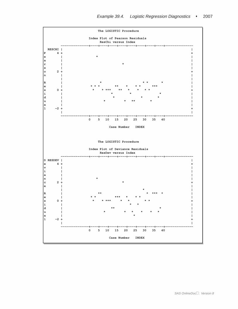
Example 39.4. Logistic Regression Diagnostics � 2007
The LOGISTIC Procedure
Index Plot of Pearson ResidualsResChi versus Index
---------------+----+----+----+----+----+----+----+----+---------------RESCHI | |
P 4 + +e | * |a | |r | * |s | |o 2 + +n | |
| |R | * * * * |e | * * * ** * * * *** |s 0 + * * *** ** * * * * +i | * * * |d | * * * |u | * * ** * |a | |l -2 + +
| |---------------+----+----+----+----+----+----+----+----+---------------
0 5 10 15 20 25 30 35 40
Case Number INDEX
The LOGISTIC Procedure
Index Plot of Deviance ResidualsResDev versus Index
---------------+----+----+----+----+----+----+----+----+---------------D RESDEV | |e 4 + +v | |i | |a | |n | * |c 2 + * +e | |
| * |R | ** * *** * |e | * * *** * * * |s 0 + * * *** * * * * +i | * * |d | ** * |u | * * * * * * |a | * |l -2 + +
| |---------------+----+----+----+----+----+----+----+----+---------------
0 5 10 15 20 25 30 35 40
Case Number INDEX
SAS OnlineDoc: Version 8

2008 � Chapter 39. The LOGISTIC Procedure
The LOGISTIC Procedure
Index Plot of Diagonal Elements of the Hat MatrixH versus Index
----------------+----+----+----+----+----+----+----+----+-----------------H | |
0.3 + +| |
H | |a | * |t | |
0.2 + +D | |i | * * * |a | * * * |g | * * |o 0.1 + * * * * +n | * ** |a | * * * * **** * *** * * |l | * * * * |
| * |0.0 + * ** * +
| |----------------+----+----+----+----+----+----+----+----+-----------------
0 5 10 15 20 25 30 35 40
Case Number INDEX
The LOGISTIC Procedure
Index Plot of Standardized Changes in the Estimate for InterceptDfBeta0 versus Index
--------------+----+----+----+----+----+----+----+----+---------------DFBETA0 | |
I 1.5 + +n | |t | |e | * |r 1.0 + * +c | |e | |p | |t 0.5 + +
| |D | * |f | * |B 0.0 + *** * *** * ** ** *** * * ** * +e | ** * ** * * * * * *** |t | * * |a | |
-0.5 + +--------------+----+----+----+----+----+----+----+----+---------------
0 5 10 15 20 25 30 35 40
Case Number INDEX
SAS OnlineDoc: Version 8

Example 39.4. Logistic Regression Diagnostics � 2009
The LOGISTIC Procedure
Index Plot of Standardized Changes in the Estimate for LogRateDfBeta1 versus Index
--------------+----+----+----+----+----+----+----+----+---------------DFBETA1 | |
0.5 + +L | |o | |g | * * |R | * * * * ** ** * * ***** |a 0.0 + ** * *** * ** ** * ** * ** * +t | * |e | * |
| |D | |f -0.5 + +B | |e | |t | * |a | * |
-1.0 + +| |--------------+----+----+----+----+----+----+----+----+---------------
0 5 10 15 20 25 30 35 40
Case Number INDEX
The LOGISTIC Procedure
Index Plot of Standardized Changes in the Estimate for LogVolumeDfBeta2 versus Index
--------------+----+----+----+----+----+----+----+----+---------------DFBETA2 | |
L 0.5 + +o | |g | |V | ** |o | * * * * ** * * * ** * ***** |l 0.0 + * ** *** ** * * * * ** ** * +u | * |m | |e | |
| |D -0.5 + +f | |B | |e | * |t | |a -1.0 + * +
| |--------------+----+----+----+----+----+----+----+----+---------------
0 5 10 15 20 25 30 35 40
Case Number INDEX
SAS OnlineDoc: Version 8

2010 � Chapter 39. The LOGISTIC Procedure
The LOGISTIC Procedure
Index Plot of Confidence Interval Displacement DiagnosticsC versus Index
----------------+----+----+----+----+----+----+----+----+-----------------C C | |o 1.5 + +n | |f | * |i | |d | |e 1.0 + * +n | |c | |e | |
| |I 0.5 + +n | |t | |e | * * * * |r | * * ** * * * * |v 0.0 + *** * * *** **** *** *** * * *** ** +a | |l ----------------+----+----+----+----+----+----+----+----+-----------------
0 5 10 15 20 25 30 35 40D
Case Number INDEX
The LOGISTIC Procedure
Index Plot of Confidence Interval Displacement DiagnosticsCBar versus Index
----------------+----+----+----+----+----+----+----+----+----------------C CBAR | |o 1.5 + +n | |f | |i | * |d | |e 1.0 + +n | * |c | |e | |
| |I 0.5 + +n | |t | |e | * * |r | * * * ** * * * * |v 0.0 + *** * * **** **** *** *** * * *** ** +a | |l ----------------+----+----+----+----+----+----+----+----+----------------
0 5 10 15 20 25 30 35 40D
Case Number INDEX
SAS OnlineDoc: Version 8

Example 39.4. Logistic Regression Diagnostics � 2011
The LOGISTIC Procedure
Index Plot of Changes in DevianceDifDev versus Index
---------------+----+----+----+----+----+----+----+----+---------------DIFDEV | |
8 + +D | |e | |l | * |t 6 + +a | * |
| |D | |e 4 + +v | |i | |a | * |n 2 + * +c | * * * * |e | * * * * * |
| ** * * * * *** * |0 + *** * *** * ** ** ** * * +
---------------+----+----+----+----+----+----+----+----+---------------0 5 10 15 20 25 30 35 40
Case Number INDEX
The LOGISTIC Procedure
Index Plot of Changes in the Pearson Chi-SquareDifChiSq versus Index
--------------+----+----+----+----+----+----+----+----+--------------DIFCHISQ | |
D 15 + +e | * |l | |t | |a | |
10 + +C | * |h | |i | |S | |q 5 + +u | |a | |r | * * |e | * * * * ** * * * |
0 + *** *** **** **** *** *** * * *** * +| |--------------+----+----+----+----+----+----+----+----+--------------
0 5 10 15 20 25 30 35 40
Case Number INDEX
SAS OnlineDoc: Version 8

2012 � Chapter 39. The LOGISTIC Procedure
The index plots of the Pearson residuals and the deviance residuals indicate that case4 and case 18 are poorly accounted for by the model. The index plot of the diagonalelements of the hat matrix suggests that case 31 is an extreme point in the designspace. The index plots of DFBETAS indicate that case 4 and case 18 are causinginstability in all three parameter estimates. The other four index plots also point tothese two cases as having a large impact on the coefficients and goodness of fit.
Example 39.5. Stratified Sampling
Consider the hypothetical example in Fleiss (1981, pp. 6–7) in which a test is appliedto a sample of 1000 people known to have a disease and to another sample of 1000people known not to have the same disease. In the diseased sample, 950 test positive;in the nondiseased sample, only 10 test positive. If the true disease rate in the popu-lation is 1 in 100, specifying PEVENT=0.01 results in the correct false positive andnegative rates for the stratified sampling scheme. Omitting the PEVENT= option isequivalent to using the overall sample disease rate (1000/2000 = 0.5) as the value ofthe PEVENT= option, which would ignore the stratified sampling.
The SAS code is as follows:
data Screen;do Disease=’Present’,’Absent’;
do Test=1,0;input Count @@;output;
end;end;datalines;
950 5010 990
;
proc logistic order=data data=Screen;freq Count;model Disease=Test / pevent=.5 .01 ctable pprob=.5;
run;
The ORDER=DATA option causes theDisease level of the first observation in theinput data set to be the event. So,Disease=’Present’ is the event. The CTABLEoption is specified to produce a classification table. Specifying PPROB=0.5 indicatesa cutoff probability of 0.5. A list of two probabilities, 0.5 and 0.01, is specified forthe PEVENT= option; 0.5 corresponds to the overall sample disease rate, and 0.01corresponds to a true disease rate of 1 in 100.
The classification table is shown in Output 39.5.1.
SAS OnlineDoc: Version 8

Example 39.6. ROC Curve, Customized Odds Ratios,... � 2013
Output 39.5.1. False Positive and False Negative Rates
The LOGISTIC Procedure
Classification Table
Correct Incorrect PercentagesProb Prob Non- Non- Sensi- Speci- False False
Event Level Event Event Event Event Correct tivity ficity POS NEG
0.500 0.500 950 990 10 50 97.0 95.0 99.0 1.0 4.8
0.010 0.500 950 990 10 50 99.0 95.0 99.0 51.0 0.1
In the classification table, the column “Prob Level” represents the cutoff values (thesettings of the PPROB= option) for predicting whether an observation is an event.The “Correct” columns list the numbers of subjects that are correctly predicted asevents and nonevents, respectively, and the “Incorrect” columns list the number ofnonevents incorrectly predicted as events and the number of events incorrectly pre-dicted as nonevents, respectively. For PEVENT=0.5, the false positive rate is 1% andthe false negative rate is 4.8%. These results ignore the fact that the samples werestratified and incorrectly assume that the overall sample proportion of disease (whichis 0.5) estimates the true disease rate. For a true disease rate of 0.01, the false posi-tive rate and the false negative rate are 51% and 0.1%, respectively, as shown on thesecond line of the classification table.
Example 39.6. ROC Curve, Customized Odds Ratios,Goodness-of-Fit Statistics, R-Square, andConfidence Limits
This example plots an ROC curve, estimates a customized odds ratio, produces thetraditional goodness-of-fit analysis, displays the generalizedR2 measures for the fit-ted model, and calculates the normal confidence intervals for the regression parame-ters. The data consist of three variables:n (number of subjects in a sample),disease(number of diseased subjects in the sample), andage (age for the sample). A lin-ear logistic regression model is used to study the effect of age on the probability ofcontracting the disease.
The SAS code is as follows:
data Data1;input disease n age;datalines;
0 14 250 20 350 19 457 18 556 12 65
17 17 75;
SAS OnlineDoc: Version 8
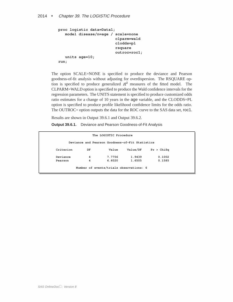
2014 � Chapter 39. The LOGISTIC Procedure
proc logistic data=Data1;model disease/n=age / scale=none
clparm=waldclodds=plrsquareoutroc=roc1;
units age=10;run;
The option SCALE=NONE is specified to produce the deviance and Pearsongoodness-of-fit analysis without adjusting for overdispersion. The RSQUARE op-tion is specified to produce generalizedR2 measures of the fitted model. TheCLPARM=WALD option is specified to produce the Wald confidence intervals for theregression parameters. The UNITS statement is specified to produce customized oddsratio estimates for a change of 10 years in theage variable, and the CLODDS=PLoption is specified to produce profile likelihood confidence limits for the odds ratio.The OUTROC= option outputs the data for the ROC curve to the SAS data set,roc1.
Results are shown in Output 39.6.1 and Output 39.6.2.
Output 39.6.1. Deviance and Pearson Goodness-of-Fit Analysis
The LOGISTIC Procedure
Deviance and Pearson Goodness-of-Fit Statistics
Criterion DF Value Value/DF Pr > ChiSq
Deviance 4 7.7756 1.9439 0.1002Pearson 4 6.6020 1.6505 0.1585
Number of events/trials observations: 6
SAS OnlineDoc: Version 8

Example 39.6. ROC Curve, Customized Odds Ratios,... � 2015
Output 39.6.2. R-Square, Confidence Intervals, and Customized Odds Ratio
Model Fit Statistics
InterceptIntercept and
Criterion Only Covariates
AIC 124.173 52.468SC 126.778 57.678-2 Log L 122.173 48.468
R-Square 0.5215 Max-rescaled R-Square 0.7394
Testing Global Null Hypothesis: BETA=0
Test Chi-Square DF Pr > ChiSq
Likelihood Ratio 73.7048 1 <.0001Score 55.3274 1 <.0001Wald 23.3475 1 <.0001
Analysis of Maximum Likelihood Estimates
StandardParameter DF Estimate Error Chi-Square Pr > ChiSq
Intercept 1 -12.5016 2.5555 23.9317 <.0001age 1 0.2066 0.0428 23.3475 <.0001
Association of Predicted Probabilities and Observed Responses
Percent Concordant 92.6 Somers’ D 0.906Percent Discordant 2.0 Gamma 0.958Percent Tied 5.4 Tau-a 0.384Pairs 2100 c 0.953
Wald Confidence Interval for Parameters
Parameter Estimate 95% Confidence Limits
Intercept -12.5016 -17.5104 -7.4929age 0.2066 0.1228 0.2904
Profile Likelihood Confidence Interval for Adjusted Odds Ratios
Effect Unit Estimate 95% Confidence Limits
age 10.0000 7.892 3.881 21.406
SAS OnlineDoc: Version 8

2016 � Chapter 39. The LOGISTIC Procedure
The ROC curve is plotted by the GPLOT procedure, and the plot is shown in Out-put 39.6.3.
symbol1 i=join v=none c=blue;proc gplot data=roc1;
title ’ROC Curve’;plot _sensit_*_1mspec_=1 / vaxis=0 to 1 by .1 cframe=ligr;
run;
Output 39.6.3. Receiver Operating Characteristic Curve
Note that the area under the ROC curve is given by the statisticc in the “Associationof Predicted Probabilities and Observed Responses” table. In this example, the areaunder the ROC curve is 0.953.
SAS OnlineDoc: Version 8

Example 39.7. Goodness-of-Fit Tests and Subpopulations � 2017
Example 39.7. Goodness-of-Fit Tests and Subpopulations
A study is done to investigate the effects of two binary factors,A andB, on a binaryresponse,Y. Subjects are randomly selected from subpopulations defined by the fourpossible combinations of levels ofA andB. The number of subjects responding witheach level ofY is recorded and entered into data setA.
data a;do A=0,1;
do B=0,1;do Y=1,2;
input F @@;output;
end;end;
end;datalines;
23 63 31 70 67 100 70 104;
A full model is fit to examine the main effects ofA andB as well as the interactioneffect ofA andB.
proc logistic data=a;freq F;model Y=A B A*B;
run;
SAS OnlineDoc: Version 8

2018 � Chapter 39. The LOGISTIC Procedure
Output 39.7.1. Full Model Fit
The LOGISTIC Procedure
Model Information
Data Set WORK.AResponse Variable YNumber of Response Levels 2Number of Observations 8Frequency Variable FSum of Frequencies 528Link Function LogitOptimization Technique Fisher’s scoring
Response Profile
Ordered TotalValue Y Frequency
1 1 1912 2 337
Model Convergence Status
Convergence criterion (GCONV=1E-8) satisfied.
Model Fit Statistics
InterceptIntercept and
Criterion Only Covariates
AIC 693.061 691.914SC 697.330 708.990-2 Log L 691.061 683.914
Testing Global Null Hypothesis: BETA=0
Test Chi-Square DF Pr > ChiSq
Likelihood Ratio 7.1478 3 0.0673Score 6.9921 3 0.0721Wald 6.9118 3 0.0748
Analysis of Maximum Likelihood Estimates
StandardParameter DF Estimate Error Chi-Square Pr > ChiSq
Intercept 1 -1.0074 0.2436 17.1015 <.0001A 1 0.6069 0.2903 4.3714 0.0365B 1 0.1929 0.3254 0.3515 0.5533A*B 1 -0.1883 0.3933 0.2293 0.6321
Association of Predicted Probabilities and Observed Responses
Percent Concordant 42.2 Somers’ D 0.118Percent Discordant 30.4 Gamma 0.162Percent Tied 27.3 Tau-a 0.054Pairs 64367 c 0.559
SAS OnlineDoc: Version 8

Example 39.7. Goodness-of-Fit Tests and Subpopulations � 2019
Pearson and Deviance goodness-of-fit tests cannot be obtained for this model since afull model containing four parameters is fit, leaving no residual degrees of freedom.For a binary response model, the goodness-of-fit tests havem�q degrees of freedom,wherem is the number of subpopulations andq is the number of model parameters.In the preceding model,m = q = 4, resulting in zero degrees of freedom for thetests.
Results of the model fit are shown in Output 39.7.1. Notice that neither theA*B in-teraction nor theB main effect is significant. If a reduced model containing only theA effect is fit, two degrees of freedom become available for testing goodness of fit.Specifying the SCALE=NONE option requests the Pearson and deviance statistics.With single-trial syntax, the AGGREGATE= option is needed to define the subpop-ulations in the study. Specifying AGGREGATE=(A B) creates subpopulations of thefour combinations of levels ofA andB. Although theB effect is being dropped fromthe model, it is still needed to define the original subpopulations in the study. If AG-GREGATE=(A) were specified, only two subpopulations would be created from thelevels ofA, resulting inm = q = 2 and zero degrees of freedom for the tests.
proc logistic data=a;freq F;model Y=A / scale=none aggregate=(A B);
run;
SAS OnlineDoc: Version 8

2020 � Chapter 39. The LOGISTIC Procedure
Output 39.7.2. Reduced Model Fit
The LOGISTIC Procedure
Model Information
Data Set WORK.AResponse Variable YNumber of Response Levels 2Number of Observations 8Frequency Variable FSum of Frequencies 528Link Function LogitOptimization Technique Fisher’s scoring
Response Profile
Ordered TotalValue Y Frequency
1 1 1912 2 337
Model Convergence Status
Convergence criterion (GCONV=1E-8) satisfied.
Deviance and Pearson Goodness-of-Fit Statistics
Criterion DF Value Value/DF Pr > ChiSq
Deviance 2 0.3541 0.1770 0.8377Pearson 2 0.3531 0.1765 0.8382
Number of unique profiles: 4
Model Fit Statistics
InterceptIntercept and
Criterion Only Covariates
AIC 693.061 688.268SC 697.330 696.806-2 Log L 691.061 684.268
Testing Global Null Hypothesis: BETA=0
Test Chi-Square DF Pr > ChiSq
Likelihood Ratio 6.7937 1 0.0091Score 6.6779 1 0.0098Wald 6.6210 1 0.0101
SAS OnlineDoc: Version 8

Example 39.8. Overdispersion � 2021
Analysis of Maximum Likelihood Estimates
StandardParameter DF Estimate Error Chi-Square Pr > ChiSq
Intercept 1 -0.9013 0.1614 31.2001 <.0001A 1 0.5032 0.1955 6.6210 0.0101
Association of Predicted Probabilities and Observed Responses
Percent Concordant 28.3 Somers’ D 0.112Percent Discordant 17.1 Gamma 0.246Percent Tied 54.6 Tau-a 0.052Pairs 64367 c 0.556
The goodness-of-fit tests (Output 39.7.2) show that dropping theB main effect andthe A*B interaction simultaneously does not result in significant lack of fit of themodel. The tests’ largep-values indicate insufficient evidence for rejecting the nullhypothesis that the model fits.
Example 39.8. Overdispersion
In a seed germination test, seeds of two cultivars were planted in pots of two soilconditions. The following SAS statements create the data setseeds, which containsthe observed proportion of seeds that germinated for various combinations of cultivarand soil condition. Variablen represents the number of seeds planted in a pot, andvariabler represents the number germinated. The indicator variablescult andsoilrepresent the cultivar and soil condition, respectively.
data seeds;input pot n r cult soil;datalines;
1 16 8 0 02 51 26 0 03 45 23 0 04 39 10 0 05 36 9 0 06 81 23 1 07 30 10 1 08 39 17 1 09 28 8 1 0
10 62 23 1 011 51 32 0 112 72 55 0 113 41 22 0 114 12 3 0 115 13 10 0 116 79 46 1 117 30 15 1 118 51 32 1 119 74 53 1 120 56 12 1 1;
SAS OnlineDoc: Version 8
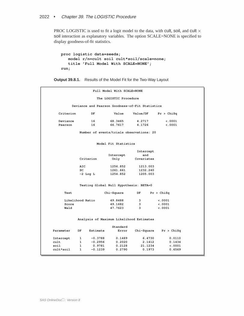
2022 � Chapter 39. The LOGISTIC Procedure
PROC LOGISTIC is used to fit a logit model to the data, withcult, soil, andcult �soil interaction as explanatory variables. The option SCALE=NONE is specified todisplay goodness-of-fit statistics.
proc logistic data=seeds;model r/n=cult soil cult*soil/scale=none;title ’Full Model With SCALE=NONE’;
run;
Output 39.8.1. Results of the Model Fit for the Two-Way Layout
Full Model With SCALE=NONE
The LOGISTIC Procedure
Deviance and Pearson Goodness-of-Fit Statistics
Criterion DF Value Value/DF Pr > ChiSq
Deviance 16 68.3465 4.2717 <.0001Pearson 16 66.7617 4.1726 <.0001
Number of events/trials observations: 20
Model Fit Statistics
InterceptIntercept and
Criterion Only Covariates
AIC 1256.852 1213.003SC 1261.661 1232.240-2 Log L 1254.852 1205.003
Testing Global Null Hypothesis: BETA=0
Test Chi-Square DF Pr > ChiSq
Likelihood Ratio 49.8488 3 <.0001Score 49.1682 3 <.0001Wald 47.7623 3 <.0001
Analysis of Maximum Likelihood Estimates
StandardParameter DF Estimate Error Chi-Square Pr > ChiSq
Intercept 1 -0.3788 0.1489 6.4730 0.0110cult 1 -0.2956 0.2020 2.1412 0.1434soil 1 0.9781 0.2128 21.1234 <.0001cult*soil 1 -0.1239 0.2790 0.1973 0.6569
SAS OnlineDoc: Version 8

Example 39.8. Overdispersion � 2023
Results of fitting the full factorial model are shown in Output 39.8.1. Both Pearson�2 and deviance are highly significant (p < 0:0001), suggesting that the model doesnot fit well. If the link function and the model specification are correct and if thereare no outliers, then the lack of fit may be due to overdispersion. Without adjustingfor the overdispersion, the standard errors are likely to be underestimated, causing theWald tests to be too sensitive. In PROC LOGISTIC, there are three SCALE= optionsto accommodate overdispersion. With unequal sample sizes for the observations,SCALE=WILLIAMS is preferred. The Williams model estimates a scale parameter� by equating the value of Pearson�2 for the full model to its approximate expectedvalue. The full model considered here is the model with cultivar, soil condition, andtheir interaction. Using a full model reduces the risk of contaminating� with lack offit due to incorrect model specification.
proc logistic data=seeds;model r/n=cult soil cult*soil / scale=williams;title ’Full Model With SCALE=WILLIAMS’;
run;
SAS OnlineDoc: Version 8

2024 � Chapter 39. The LOGISTIC Procedure
Output 39.8.2. Williams’ Model for Overdispersion
Full Model With SCALE=WILLIAMS
The LOGISTIC Procedure
Model Information
Data Set WORK.SEEDSResponse Variable (Events) rResponse Variable (Trials) nNumber of Observations 20Weight Variable 1 / ( 1 + 0.075941 * (n - 1) )Sum of Weights 198.32164573Link Function LogitOptimization Technique Fisher’s scoring
Response Profile
Ordered Binary Total TotalValue Outcome Frequency Weight
1 Event 437 92.953462 Nonevent 469 105.36819
Model Convergence Status
Convergence criterion (GCONV=1E-8) satisfied.
Deviance and Pearson Goodness-of-Fit Statistics
Criterion DF Value Value/DF Pr > ChiSq
Deviance 16 16.4402 1.0275 0.4227Pearson 16 16.0000 1.0000 0.4530
Number of events/trials observations: 20
NOTE: Since the Williams method was used to accomodate overdispersion, thePearson chi-squared statistic and the deviance can no longer be used toassess the goodness of fit of the model.
Model Fit Statistics
InterceptIntercept and
Criterion Only Covariates
AIC 276.155 273.586SC 280.964 292.822-2 Log L 274.155 265.586
Testing Global Null Hypothesis: BETA=0
Test Chi-Square DF Pr > ChiSq
Likelihood Ratio 8.5687 3 0.0356Score 8.4856 3 0.0370Wald 8.3069 3 0.0401
SAS OnlineDoc: Version 8

Example 39.8. Overdispersion � 2025
Analysis of Maximum Likelihood Estimates
StandardParameter DF Estimate Error Chi-Square Pr > ChiSq
Intercept 1 -0.3926 0.2932 1.7932 0.1805cult 1 -0.2618 0.4160 0.3963 0.5290soil 1 0.8309 0.4223 3.8704 0.0491cult*soil 1 -0.0532 0.5835 0.0083 0.9274
Association of Predicted Probabilities and Observed Responses
Percent Concordant 50.6 Somers’ D 0.258Percent Discordant 24.8 Gamma 0.343Percent Tied 24.6 Tau-a 0.129Pairs 204953 c 0.629
Results using Williams’ method are shown in Output 39.8.2. The estimate of� is0.075941 and is given in the formula for the Weight Variable at the beginning of thedisplayed output. Since neithercult norcult times soil is statistically significant (p =0:5290 andp = 0:9274, respectively), a reduced model that contains only the soilcondition factor is fitted, with the observations weighted by1=(1+0:075941(N�1)).This can be done conveniently in PROC LOGISTIC by including the scale estimatein the SCALE=WILLIAMS option as follows:
proc logistic data=seeds;model r/n=soil / scale=williams(0.075941);title ’Reduced Model With SCALE=WILLIAMS(0.075941)’;
run;
Output 39.8.3. Reduced Model with Overdispersion Controlled
Analysis of Maximum Likelihood Estimates
StandardParameter DF Estimate Error Chi-Square Pr > ChiSq
Intercept 1 -0.5249 0.2076 6.3949 0.0114soil 1 0.7910 0.2902 7.4284 0.0064
Results of the reduced model fit are shown in Output 39.8.3. Soil condition remainsa significant factor (p = 0:0064) for the seed germination.
SAS OnlineDoc: Version 8

2026 � Chapter 39. The LOGISTIC Procedure
Example 39.9. Conditional Logistic Regression for MatchedPairs Data
In matched case-control studies, conditional logistic regression is used to investigatethe relationship between an outcome of being a case or a control and a set of prog-nostic factors. When each matched set consists of a single case and a single control,the conditional likelihood is given by
Yi
(1 + exp(��0(xi1 � xi0))�1
wherexi1 andxi0 are vectors representing the prognostic factors for the case andcontrol, respectively, of theith matched set. This likelihood is identical to the like-lihood of fitting a logistic regression model to a set of data with constant response,where the model contains no intercept term and has explanatory variables given bydi = xi1 � xi0 (Breslow 1982).
The data in this example are a subset of the data from the Los Angeles Study of theEndometrial Cancer Data in Breslow and Days (1980). There are 63 matched pairs,each consisting of a case of endometrial cancer (Outcome=1) and a control (Out-come=0). The case and corresponding control have the sameID. Two prognosticfactors are included:Gall (an indicator variable for gall bladder disease) andHy-per (an indicator variable for hypertension). The goal of the case-control analysisis to determine the relative risk for gall bladder disease, controlling for the effect ofhypertension.
Before PROC LOGISTIC is used for the logistic regression analysis, each matchedpair is transformed into a single observation, where the variablesGall andHypercontain the differences between the corresponding values for the case and the control(case� control). The variableOutcome, which will be used as the response variablein the logistic regression model, is given a constant value of 0 (which is theOutcomevalue for the control, although any constant, numeric or character, will do).
data Data1;drop id1 gall1 hyper1;retain id1 gall1 hyper1 0;input ID Outcome Gall Hyper @@ ;if (ID = id1) then do;
Gall=gall1-Gall; Hyper=hyper1-Hyper;output;
end;else do;
id1=ID; gall1=Gall; hyper1=Hyper;end;datalines;
1 1 0 0 1 0 0 0 2 1 0 0 2 0 0 03 1 0 1 3 0 0 1 4 1 0 0 4 0 1 05 1 1 0 5 0 0 1 6 1 0 1 6 0 0 07 1 1 0 7 0 0 0 8 1 1 1 8 0 0 19 1 0 0 9 0 0 0 10 1 0 0 10 0 0 0
11 1 1 0 11 0 0 0 12 1 0 0 12 0 0 1
SAS OnlineDoc: Version 8

Example 39.9. Conditional Logistic Regression � 2027
13 1 1 0 13 0 0 1 14 1 1 0 14 0 1 015 1 1 0 15 0 0 1 16 1 0 1 16 0 0 017 1 0 0 17 0 1 1 18 1 0 0 18 0 1 119 1 0 0 19 0 0 1 20 1 0 1 20 0 0 021 1 0 0 21 0 1 1 22 1 0 1 22 0 0 123 1 0 1 23 0 0 0 24 1 0 0 24 0 0 025 1 0 0 25 0 0 0 26 1 0 0 26 0 0 127 1 1 0 27 0 0 1 28 1 0 0 28 0 0 129 1 1 0 29 0 0 0 30 1 0 1 30 0 0 031 1 0 1 31 0 0 0 32 1 0 1 32 0 0 033 1 0 1 33 0 0 0 34 1 0 0 34 0 0 035 1 1 1 35 0 1 1 36 1 0 0 36 0 0 137 1 0 1 37 0 0 0 38 1 0 1 38 0 0 139 1 0 1 39 0 0 1 40 1 0 1 40 0 0 041 1 0 0 41 0 0 0 42 1 0 1 42 0 1 043 1 0 0 43 0 0 1 44 1 0 0 44 0 0 045 1 1 0 45 0 0 0 46 1 0 0 46 0 0 047 1 1 1 47 0 0 0 48 1 0 1 48 0 0 049 1 0 0 49 0 0 0 50 1 0 1 50 0 0 151 1 0 0 51 0 0 0 52 1 0 1 52 0 0 153 1 0 1 53 0 0 0 54 1 0 1 54 0 0 055 1 1 0 55 0 0 0 56 1 0 0 56 0 0 057 1 1 1 57 0 1 0 58 1 0 0 58 0 0 059 1 0 0 59 0 0 0 60 1 1 1 60 0 0 061 1 1 0 61 0 1 0 62 1 0 1 62 0 0 063 1 1 0 63 0 0 0;
Note that there are 63 observations in the data set, one for each matched pair. ThevariableOutcome has a constant value of 0.
In the following SAS statements, PROC LOGISTIC is invoked with the NOINT op-tion to obtain the conditional logistic model estimates. Two models are fitted. Thefirst model containsGall as the only predictor variable, and the second model con-tains bothGall andHyper as predictor variables. Because the option CLODDS=PLis specified, PROC LOGISTIC computes a 95% profile likelihood confidence intervalfor the odds ratio for each predictor variable.
proc logistic data=Data1;model outcome=Gall / noint CLODDS=PL;
run;
proc logistic data=Data1;model outcome=Gall Hyper / noint CLODDS=PL;
run;
Results from the two conditional logistic analyses are shown in Output 39.9.1 andOutput 39.9.2. Note that there is only one response level listed in the “ResponseProfile” tables and there is no intercept term in the “Analysis of Maximum LikelihoodEstimates” tables.
SAS OnlineDoc: Version 8

2028 � Chapter 39. The LOGISTIC Procedure
Output 39.9.1. Conditional Logistic Regression (Gall as risk factor)
The LOGISTIC Procedure
Model Information
Data Set WORK.DATA1Response Variable OutcomeNumber of Response Levels 1Number of Observations 63Link Function LogitOptimization Technique Fisher’s scoring
Response Profile
Ordered TotalValue Outcome Frequency
1 0 63
Model Convergence Status
Convergence criterion (GCONV=1E-8) satisfied.
Model Fit Statistics
Without WithCriterion Covariates Covariates
AIC 87.337 85.654SC 87.337 87.797-2 Log L 87.337 83.654
Testing Global Null Hypothesis: BETA=0
Test Chi-Square DF Pr > ChiSq
Likelihood Ratio 3.6830 1 0.0550Score 3.5556 1 0.0593Wald 3.2970 1 0.0694
Analysis of Maximum Likelihood Estimates
StandardParameter DF Estimate Error Chi-Square Pr > ChiSq
Gall 1 0.9555 0.5262 3.2970 0.0694
NOTE: Since there is only one response level, measures of association betweenthe observed and predicted values were not calculated.
Profile Likelihood Confidence Interval for Adjusted Odds Ratios
Effect Unit Estimate 95% Confidence Limits
Gall 1.0000 2.600 0.981 8.103
SAS OnlineDoc: Version 8

Example 39.9. Conditional Logistic Regression � 2029
Output 39.9.2. Conditional Logistic Regression (Gall and Hyper as risk factors)
The LOGISTIC Procedure
Model Information
Data Set WORK.DATA1Response Variable OutcomeNumber of Response Levels 1Number of Observations 63Link Function LogitOptimization Technique Fisher’s scoring
Response Profile
Ordered TotalValue Outcome Frequency
1 0 63
Model Convergence Status
Convergence criterion (GCONV=1E-8) satisfied.
Model Fit Statistics
Without WithCriterion Covariates Covariates
AIC 87.337 86.788SC 87.337 91.074-2 Log L 87.337 82.788
Testing Global Null Hypothesis: BETA=0
Test Chi-Square DF Pr > ChiSq
Likelihood Ratio 4.5487 2 0.1029Score 4.3620 2 0.1129Wald 4.0060 2 0.1349
Analysis of Maximum Likelihood Estimates
StandardParameter DF Estimate Error Chi-Square Pr > ChiSq
Gall 1 0.9704 0.5307 3.3432 0.0675Hyper 1 0.3481 0.3770 0.8526 0.3558
NOTE: Since there is only one response level, measures of association betweenthe observed and predicted values were not calculated.
Profile Likelihood Confidence Interval for Adjusted Odds Ratios
Effect Unit Estimate 95% Confidence Limits
Gall 1.0000 2.639 0.987 8.299Hyper 1.0000 1.416 0.682 3.039
SAS OnlineDoc: Version 8
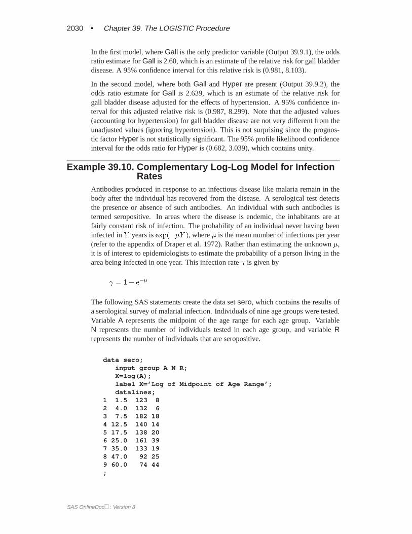
2030 � Chapter 39. The LOGISTIC Procedure
In the first model, whereGall is the only predictor variable (Output 39.9.1), the oddsratio estimate forGall is 2.60, which is an estimate of the relative risk for gall bladderdisease. A 95% confidence interval for this relative risk is (0.981, 8.103).
In the second model, where bothGall andHyper are present (Output 39.9.2), theodds ratio estimate forGall is 2.639, which is an estimate of the relative risk forgall bladder disease adjusted for the effects of hypertension. A 95% confidence in-terval for this adjusted relative risk is (0.987, 8.299). Note that the adjusted values(accounting for hypertension) for gall bladder disease are not very different from theunadjusted values (ignoring hypertension). This is not surprising since the prognos-tic factorHyper is not statistically significant. The 95% profile likelihood confidenceinterval for the odds ratio forHyper is (0.682, 3.039), which contains unity.
Example 39.10. Complementary Log-Log Model for InfectionRates
Antibodies produced in response to an infectious disease like malaria remain in thebody after the individual has recovered from the disease. A serological test detectsthe presence or absence of such antibodies. An individual with such antibodies istermed seropositive. In areas where the disease is endemic, the inhabitants are atfairly constant risk of infection. The probability of an individual never having beeninfected inY years isexp(��Y ), where� is the mean number of infections per year(refer to the appendix of Draper et al. 1972). Rather than estimating the unknown�,it is of interest to epidemiologists to estimate the probability of a person living in thearea being infected in one year. This infection rate is given by
= 1� e��
The following SAS statements create the data setsero, which contains the results ofa serological survey of malarial infection. Individuals of nine age groups were tested.Variable A represents the midpoint of the age range for each age group. VariableN represents the number of individuals tested in each age group, and variableRrepresents the number of individuals that are seropositive.
data sero;input group A N R;X=log(A);label X=’Log of Midpoint of Age Range’;datalines;
1 1.5 123 82 4.0 132 63 7.5 182 184 12.5 140 145 17.5 138 206 25.0 161 397 35.0 133 198 47.0 92 259 60.0 74 44;
SAS OnlineDoc: Version 8
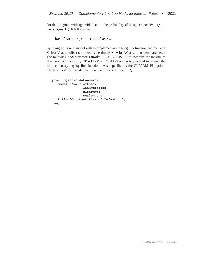
Example 39.10. Complementary Log-Log Model for Infection Rates � 2031
For theith group with age midpointAi, the probability of being seropositive ispi =1� exp(��Ai). It follows that
log(� log(1� pi)) = log(u) + log(Ai)
By fitting a binomial model with a complementary log-log link function and by usingX=log(A) as an offset term, you can estimate�0 = log(�) as an intercept parameter.The following SAS statements invoke PROC LOGISTIC to compute the maximumlikelihood estimate of�0. The LINK=CLOGLOG option is specified to request thecomplementary log-log link function. Also specified is the CLPARM=PL option,which requests the profile likelihood confidence limits for�0.
proc logistic data=sero;model R/N= / offset=X
link=cloglogclparm=plscale=none;
title ’Constant Risk of Infection’;run;
SAS OnlineDoc: Version 8
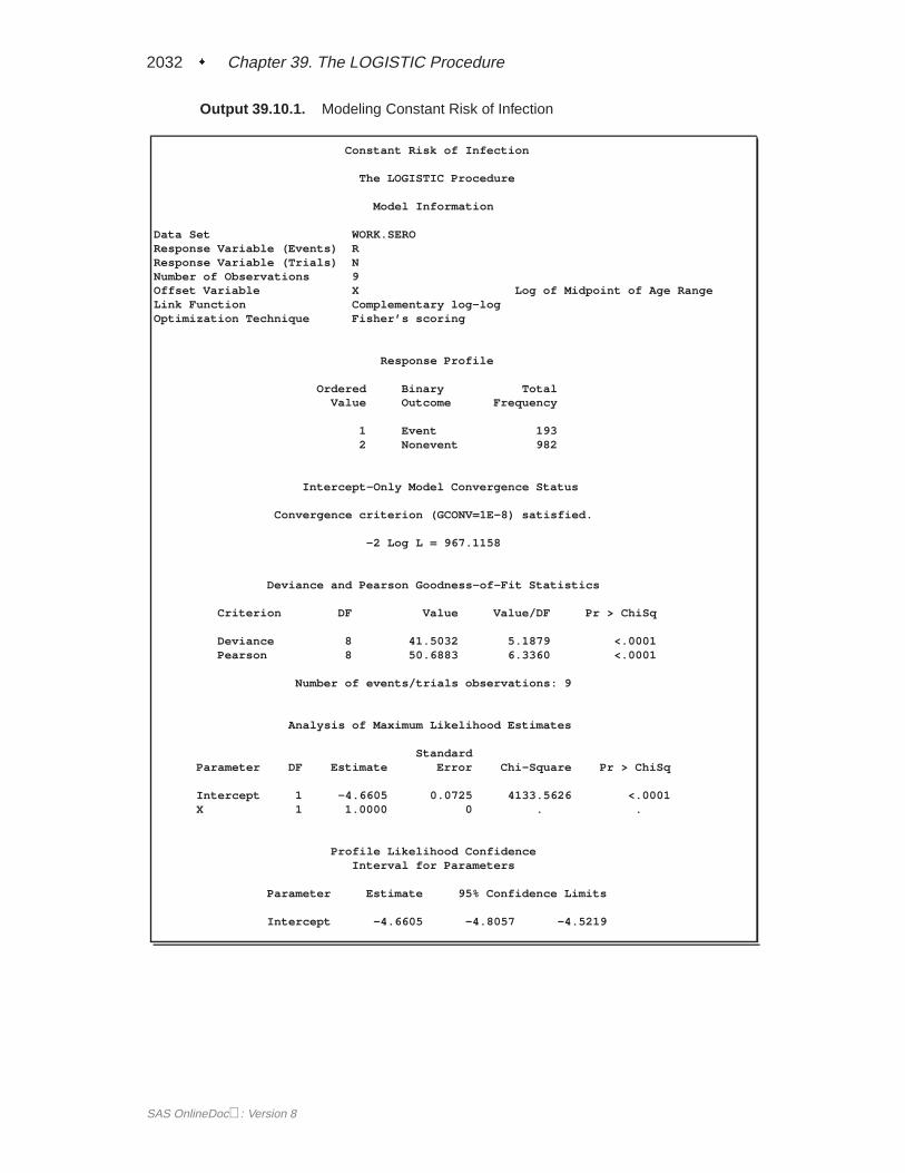
2032 � Chapter 39. The LOGISTIC Procedure
Output 39.10.1. Modeling Constant Risk of Infection
Constant Risk of Infection
The LOGISTIC Procedure
Model Information
Data Set WORK.SEROResponse Variable (Events) RResponse Variable (Trials) NNumber of Observations 9Offset Variable X Log of Midpoint of Age RangeLink Function Complementary log-logOptimization Technique Fisher’s scoring
Response Profile
Ordered Binary TotalValue Outcome Frequency
1 Event 1932 Nonevent 982
Intercept-Only Model Convergence Status
Convergence criterion (GCONV=1E-8) satisfied.
-2 Log L = 967.1158
Deviance and Pearson Goodness-of-Fit Statistics
Criterion DF Value Value/DF Pr > ChiSq
Deviance 8 41.5032 5.1879 <.0001Pearson 8 50.6883 6.3360 <.0001
Number of events/trials observations: 9
Analysis of Maximum Likelihood Estimates
StandardParameter DF Estimate Error Chi-Square Pr > ChiSq
Intercept 1 -4.6605 0.0725 4133.5626 <.0001X 1 1.0000 0 . .
Profile Likelihood ConfidenceInterval for Parameters
Parameter Estimate 95% Confidence Limits
Intercept -4.6605 -4.8057 -4.5219
SAS OnlineDoc: Version 8

Example 39.10. Complementary Log-Log Model for Infection Rates � 2033
Results of fitting this constant risk model are shown in Output 39.10.1. The maximumlikelihood estimate of�0 = log(�) and its estimated standard error areb�0 = �4:6605andb�
b�0= 0:0725, respectively. The infection rate is estimated as
b = 1� e�b� = 1� e�eb�0= 1� e�e
�4:6605= 0:00942
The 95% confidence interval for , obtained by back-transforming the 95% confi-dence interval for�0, is (0.0082, 0.0011); that is, there is a 95% chance that, in re-peated sampling, the interval of 8 to 11 infections per thousand individuals containsthe true infection rate.
The goodness of fit statistics for the constant risk model are statistically significant(p < 0:0001), indicating that the assumption of constant risk of infection is not cor-rect. You can fit a more extensive model by allowing a separate risk of infection foreach age group. Suppose�i is the mean number of infections per year for theithage group. The probability of seropositive for theith group with age midpointAi ispi = 1� exp(��iAi), so that
log(� log(1� pi) = log(�i) + log(Ai)
In the following SAS statements, nine dummy variables (agegrp1–agegrp9) arecreated as the design variables for the age groups. PROC LOGISTIC is invokedto fit a complementary log-log model that containsagegrp1–agegrp9 as the onlyexplanatory variables with no intercept term and with X=log(A) as an offset term.Note thatlog(�i) is the regression parameter associated withagegrpi.
data two;array agegrp(9) agegrp1-agegrp9 (0 0 0 0 0 0 0 0 0);set sero;agegrp[group]=1;output;agegrp[group]=0;
run;proc logistic data=two;
model R/N=agegrp1-agegrp9 / offset=Xnointlink=cloglogclparm=pl;
title ’Infectious Rates and 95% Confidence Intervals’;run;
SAS OnlineDoc: Version 8

2034 � Chapter 39. The LOGISTIC Procedure
Output 39.10.2. Modeling Separate Risk of Infection
Infectious Rates and 95% Confidence Intervals
The LOGISTIC Procedure
Analysis of Maximum Likelihood Estimates
StandardParameter DF Estimate Error Chi-Square Pr > ChiSq
agegrp1 1 -3.1048 0.3536 77.0877 <.0001agegrp2 1 -4.4542 0.4083 119.0164 <.0001agegrp3 1 -4.2769 0.2358 328.9593 <.0001agegrp4 1 -4.7761 0.2674 319.0600 <.0001agegrp5 1 -4.7165 0.2238 443.9920 <.0001agegrp6 1 -4.5012 0.1606 785.1350 <.0001agegrp7 1 -5.4252 0.2296 558.1114 <.0001agegrp8 1 -4.9987 0.2008 619.4666 <.0001agegrp9 1 -4.1965 0.1559 724.3157 <.0001X 1 1.0000 0 . .
Profile Likelihood ConfidenceInterval for Parameters
Parameter Estimate 95% Confidence Limits
agegrp1 -3.1048 -3.8880 -2.4833agegrp2 -4.4542 -5.3769 -3.7478agegrp3 -4.2769 -4.7775 -3.8477agegrp4 -4.7761 -5.3501 -4.2940agegrp5 -4.7165 -5.1896 -4.3075agegrp6 -4.5012 -4.8333 -4.2019agegrp7 -5.4252 -5.9116 -5.0063agegrp8 -4.9987 -5.4195 -4.6289agegrp9 -4.1965 -4.5164 -3.9037
Table 39.3. Infection Rate in One Year
Number Infected per 1000 PeopleAge Point 95% Confidence Limits
Group Estimate Lower Upper1 44 20 802 12 5 233 14 8 214 8 5 145 9 6 136 11 8 157 4 3 78 7 4 109 15 11 20
Results of fitting the model for separate risk of infection are shown in Output 39.10.2.For the first age group, the point estimate oflog(�1) is �3:1048. This translatesinto an infection rate of1 � exp(� exp(�3:1048)) = 0:0438. A 95% confidenceinterval for the infection rate is obtained by transforming the 95% confidence inter-val for log(�1). For the first age group, the lower and upper confidence limits are1 � exp(� exp(�3:8880) = 0:0203 and1 � exp(� exp(�2:4833)) = 0:0801, re-spectively. Table 39.3 on page 2034 shows the estimated infection rate in one year’stime for each age group. Note that the infection rate for the first age group is highcompared to the other age groups.
SAS OnlineDoc: Version 8

Example 39.11. Complementary Log-Log Model for Interval-censored SurvivalTimes � 2035
Example 39.11. Complementary Log-Log Model forInterval-censored Survival Times
Often survival times are not observed more precisely than the interval (for instance,a day) within which the event occurred. Survival data of this form are known asgrouped or interval-censored data. A discrete analogue of the continuous proportionalhazards model (Prentice and Gloeckler 1978; Allison 1982) is used to investigate therelationship between these survival times and a set of explanatory variables.
SupposeTi is the discrete survival time variable of theith subject with covariatesxi.The discrete-time hazard rate�it is defined as
�it = Pr(Ti = t j Ti � t;xi); t = 1; 2; : : :
Using elementary properties of conditional probabilities, it can be shown that
Pr(Ti = t) = �it
t�1Yj=1
(1� �ij) and Pr(Ti > t) =tY
j=1
(1� �ij)
Supposeti is the observed survival time of theith subject. Suppose�i = 1 if Ti = tiis an event time and 0 otherwise. The likelihood for the grouped survival data is givenby
L =Yi
[Pr(Ti = ti)]�ifPr(Ti > ti)]
1��i
=Yi
��iti
1� �iti
��i tiYj=1
(1� �ij)
=Yi
tiYj=1
��ij
1� �ij
�yij
(1� �ij)
whereyij = 1 if the ith subject experienced an event at timeTi = j and 0 otherwise.
Note that the likelihoodL for the grouped survival data is the same as the likelihoodof a binary response model with event probabilities�ij. If the data are generated bya continuous-time proportional hazards model, Prentice and Gloeckler (1978) haveshown that
�ij = 1� exp(� exp(�j + �0xi))
where the coefficient vector� is identical to that of the continuous-time proportionalhazards model, and�j is a constant related to the conditional survival probabilityin the interval defined byTi = j at xi = 0. The grouped data survival modelis therefore equivalent to the binary response model with complementary log-loglink function. To fit the grouped survival model using PROC LOGISTIC, you musttreat each discrete time unit for each subject as a separate observation. For each of
SAS OnlineDoc: Version 8

2036 � Chapter 39. The LOGISTIC Procedure
these observations, the response is dichotomous, corresponding to whether or not thesubject died in the time unit.
Consider a study of the effect of insecticide on flour-beetles. Four different con-centrations of an insecticide were sprayed on separate groups of flour-beetles. Thenumbers of male and female flour-beetles dying in successive intervals were saved inthe data setbeetles.
data beetles(keep=time sex conc freq);input time m20 f20 m32 f32 m50 f50 m80 f80;conc=.20;freq= m20; sex=1; output;freq= f20; sex=2; output;conc=.32;freq= m32; sex=1; output;freq= f32; sex=2; output;conc=.50;freq= m50; sex=1; output;freq= f50; sex=2; output;conc=.80;freq= m80; sex=1; output;freq= f80; sex=2; output;datalines;
1 3 0 7 1 5 0 4 22 11 2 10 5 8 4 10 73 10 4 11 11 11 6 8 154 7 8 16 10 15 6 14 95 4 9 3 5 4 3 8 36 3 3 2 1 2 1 2 47 2 0 1 0 1 1 1 18 1 0 0 1 1 4 0 19 0 0 1 1 0 0 0 0
10 0 0 0 0 0 0 1 111 0 0 0 0 1 1 0 012 1 0 0 0 0 1 0 013 1 0 0 0 0 1 0 014 101 126 19 47 7 17 2 4;
The data setbeetles contains four variables:time, sex, conc, andfreq. time repre-sents the interval death time; for example,time=2 is the interval between day 1 andday 2. Insects surviving the duration (13 days) of the experiment are given atimevalue of 14. The variablesex represents the sex of the insects (1=male, 2=female),conc represents the concentration of the insecticide (mg/cm2), and freq representsthe frequency of the observations.
To use PROC LOGISTIC with the grouped survival data, you must expand the dataso that each beetle has a separate record for each day of survival. A beetle that diedin the third day (time=3) would contribute three observations to the analysis, one foreach day it was alive at the beginning of the day. A beetle that survives the 13-dayduration of the experiment (time=14) would contribute 13 observations.
SAS OnlineDoc: Version 8

Example 39.11. Complementary Log-Log Model for Interval-censored SurvivalTimes � 2037
A new data setdays that contains the beetle-day observations is created from the datasetbeetles. In addition to the variablessex, conc andfreq, the data set contains anoutcome variabley and 13 indicator variablesday1, day2, : : :, day13. y has a valueof 1 if the observation corresponds to the day that the beetle died and has a value of0 otherwise. An observation for the first day will have a value of 1 forday1 and avalue of 0 forday2–day13; an observation for the second day will have a value of 1for day2 and a value of 0 forday1 andday2–day13. For instance, Output 39.11.1shows an observation in thebeetles data set withtime=3, and Output 39.11.2 showsthe corresponding beetle-day observations in the data setdays.
data days;retain day1-day13 0;array dd[13] day1-day13;set beetles;if time = 14 then do day=1 to 13;
y=0; dd[day]=1;output;dd[day]=0;
end;else do day=1 to time;
if day=time then y=1;else y=0;dd[day]=1;output;dd[day]=0;
end;
Output 39.11.1. An Observation with Time=3 in Data Set Beetles
Obs time conc freq sex
17 3 0.2 10 1
Output 39.11.2. Corresponding Beetle-day Observations in Days
d d d dt c f d d d d d d d d d a a a a
O i o r s d a a a a a a a a a y y y yb m n e e a y y y y y y y y y 1 1 1 1s e c q x y y 1 2 3 4 5 6 7 8 9 0 1 2 3
25 3 0.2 10 1 1 0 1 0 0 0 0 0 0 0 0 0 0 0 026 3 0.2 10 1 2 0 0 1 0 0 0 0 0 0 0 0 0 0 027 3 0.2 10 1 3 1 0 0 1 0 0 0 0 0 0 0 0 0 0
The following SAS statements invoke PROC LOGISTIC to fit a complementarylog-log model for binary data with response variable Y and explanatory variablesday1–day13, sex, andconc. Since the values ofy are coded 0 and 1, specifying theDESCENDING option ensures that the event (y=1) probability is modeled. The co-efficients ofday1–day13 can be used to estimate the baseline survival function. TheNOINT option is specified to prevent any redundancy in estimating the coefficients ofday1–day13. The Newton-Raphson algorithm is used for the maximum likelihoodestimation of the parameters.
SAS OnlineDoc: Version 8

2038 � Chapter 39. The LOGISTIC Procedure
proc logistic data=days descending outest=est1;model y= day1-day13 sex conc / noint link=cloglog
technique=newton;freq freq;
run;
Output 39.11.3. Parameter Estimates for the Grouped Proportional HazardsModel
Analysis of Maximum Likelihood Estimates
StandardParameter DF Estimate Error Chi-Square Pr > ChiSq
day1 1 -3.9314 0.2934 179.5602 <.0001day2 1 -2.8751 0.2412 142.0596 <.0001day3 1 -2.3985 0.2299 108.8833 <.0001day4 1 -1.9953 0.2239 79.3960 <.0001day5 1 -2.4920 0.2515 98.1470 <.0001day6 1 -3.1060 0.3037 104.5799 <.0001day7 1 -3.9704 0.4230 88.1107 <.0001day8 1 -3.7917 0.4007 89.5233 <.0001day9 1 -5.1540 0.7316 49.6329 <.0001day10 1 -5.1350 0.7315 49.2805 <.0001day11 1 -5.1131 0.7313 48.8834 <.0001day12 1 -5.1029 0.7313 48.6920 <.0001day13 1 -5.0951 0.7313 48.5467 <.0001sex 1 -0.5651 0.1141 24.5477 <.0001conc 1 3.0918 0.2288 182.5665 <.0001
Results of the model fit are given in Output 39.11.3. Bothsex andconc are statisti-cally significant for the survival of beetles sprayed by the insecticide. Female beetlesare more resilient to the chemical than male beetles, and increased concentration in-creases the effectiveness of the insecticide.
The coefficients of day1–day13 are the maximum likelihood estimates of�1; : : : ; �13, respectively. The baseline survivor functionS0(t) is estimated by
S0(t) = cPr(T > t) =Yj�t
exp(� exp(�j))
and the survivor function for a given covariate pattern (sex=x1 and conc=x2) isestimated by
S(t) = [S0(t)]exp(�0:5651x1+3:0918x2)
The following DATA step computes the survivor curves for male and female flour-beetles exposed to the insecticide of concentrations .20 mg/cm2 and .80 mg/cm2.The GPLOT procedure in SAS/GRAPH software is used to plot the survival curves.Instead of plotting them as step functions, the SPLINE option is used to smooth thecurves. These smoothed survival curves are displayed in Output 39.11.4.
SAS OnlineDoc: Version 8

Example 39.11. Complementary Log-Log Model for Interval-censored SurvivalTimes � 2039
data one (keep=day survival element s_m20 s_f20 s_m80 s_f80);array dd day1-day13;array sc[4] m20 f20 m80 f80;array s_sc[4] s_m20 s_f20 s_m80 s_f80 (1 1 1 1);set est1;m20= exp(sex + .20 * conc);f20= exp(2 * sex + .20 * conc);m80= exp(sex + .80 * conc);f80= exp(2 * sex + .80 * conc);survival=1;day=0;output;do over dd;
element= exp(-exp(dd));survival= survival * element;do i=1 to 4;
s_sc[i] = survival ** sc[i];end;day + 1;output;
end;label s_m20= ’Male at .20 conc.’
s_m80= ’Male at .80 conc.’s_f20= ’Female at .20 conc.’s_f80= ’Female at .80 conc.’;
run;
title1 ’Flour-Beetles Sprayed with Insecticide’;legend1 label=none frame cframe=ligr cborder=black
position=center value=(justify=center);axis1 label=(angle=90 ’Survival Function’);
proc gplot data=one;plot (s_m20 s_f20 s_m80 s_f80) * day
/ overlay legend=legend1 vaxis=axis1 cframe=ligr;symbol1 v=dot i=spline c=black height=.8;symbol2 v=dot i=spline c=red height=.8;symbol3 v=dot i=spline c=blue height=.8;symbol4 v=dot i=spline c=yellow height=.8;
run;
The probability of survival is displayed on the vertical axis. Notice that most of theinsecticide effect occurs by day 6 for both the high and low concentrations.
SAS OnlineDoc: Version 8

2040 � Chapter 39. The LOGISTIC Procedure
Output 39.11.4. Predicted Survival at Concentrations of 0.20 and 0.80 mg/cm2
References
Agresti, A. (1984),Analysis of Ordinal Categorical Data, New York: John Wiley &Sons, Inc.
Agresti, A. (1990),Categorical Data Analysis, New York: John Wiley & Sons, Inc.
Aitchison, J. and Silvey, S.D. ( 1957), “The Generalization of Probit Analysis to theCase of Multiple Responses,”Biometrika, 44, 131–40.
Albert, A. and Anderson, J.A. (1984), “On the Existence of Maximum LikelihoodEstimates in Logistic Regression Models,”Biometrika, 71, 1–10.
Allison, P.D. (1982), “Discrete-Time Methods for the Analysis of Event Histories,” inSociological Methods and Research, 15, ed S. Leinhardt, San Francisco: Jossey-Bass, 61–98.
Ashford, J.R. (1959), “An Approach to the Analysis of Data for Semi-Quantal Re-sponses in Biology Response,”Biometrics, 15, 573–81.
Bartolucci, A.A. and Fraser, M.D. (1977), “Comparative Step-Up and CompositeTest for Selecting Prognostic Indicator Associated with Survival,”BiometricalJournal, 19, 437–448.
Breslow, N.E. and Days W. (1980),Statistical Methods in Cancer Research, Volume1–The Analysis of Case-Control Studies, Lyon: IARC Scientific Publication No.32.
Breslow, N.E. (1982), “Covariance Adjustment of Relative-Risk Estimates inMatched Studies,”Biometrics, 38, 661–672.
SAS OnlineDoc: Version 8

References � 2041
Collett, D. (1991),Modelling Binary Data, London: Chapman and Hall.
Cook, R.D. and Weisberg, S. (1982),Residuals and Influence in Regression, NewYork: Chapman and Hall.
Cox, D.R. and Snell, E.J. (1989),The Analysis of Binary Data, Second Edition, Lon-don: Chapman and Hall.
DeLong, E.R., DeLong, D.M., and Clarke-Pearson, D.L. (1988), “Comparing theAreas Under Two or More Correlated Receiver Operating Characteristic Curves:a Nonparametric Approach,”Biometrics, 44, 837–845.
Draper, C.C., Voller, A., and Carpenter, R.G. (1972), “The Epidemiologic Interpreta-tion of Serologic Data in Malaria,”American Journal of Tropical Medicine andHygiene, 21, 696–703.
Finney, D.J. (1947), “The Estimation from Individual Records of the Relationshipbetween Dose and Quantal Response,”Biometrika, 34, 320–334.
Fleiss, J.L. (1981),Statistical Methods for Rates and Proportions, Second Edition,New York: John Wiley & Sons, Inc.
Freeman, D.H., Jr. (1987),Applied Categorical Data Analysis, New York: MarcelDekker, Inc.
Furnival, G.M. and Wilson, R.W. (1974), “Regressions by Leaps and Bounds,”Tech-nometrics, 16, 499–511.
Hanley, J.A. and McNeil, B.J. (1982), “The Meaning and Use of the Area under aReceiver Operating Characteristic (ROC) Curve,”Radiology, 143 29–36.
Harrell, F.E. (1986), “The LOGIST Procedure,”SUGI Supplemental Library Guide,Version 5 Edition, Cary, NC: SAS Institute Inc.
Hosmer, D.W, Jr. and Lemeshow, S. (1989),Applied Logistic Regression, New York:John Wiley & Sons, Inc.
Lawless, J.F. and Singhal, K. (1978), “Efficient Screening of Nonnormal RegressionModels,”Biometrics, 34, 318–327.
Lee, E.T. (1974), “A Computer Program for Linear Logistic Regression Analysis,”Computer Programs in Biomedicine, 80–92.
McCullagh, P. and Nelder, J.A. (1989),Generalized Linear Models, London: Chap-man Hall.
Nagelkerke, N.J.D. (1991), “A Note on a General Definition of the Coefficient ofDetermination,”Biometrika, 78, 691–692.
Nelder, J.A. and Wedderburn, R.W.M. (1972), “Generalized Linear Models,”Journalof the Royal Statistical Society, Series A, 135, 761–768.
Pregibon, D. (1981), “Logistic Regression Diagnostics,”Annals of Statistics, 9,705–724.
Prentice, P.L. and Gloeckler, L.A. (1978), “Regression Analysis of Grouped SurvivalData with Applications to Breast Cancer Data,”Biometrics, 34, 57–67.
SAS OnlineDoc: Version 8

2042 � Chapter 39. The LOGISTIC Procedure
Press, S.J. and Wilson, S. (1978), “Choosing Between Logistic Regression andDiscriminant Analysis,”Journal of the American Statistical Association, 73,699–705.
Santner, T.J. and Duffy, E.D. (1986), “A Note on A. Albert and J.A. Anderson’sConditions for the Existence of Maximum Likelihood Estimates in Logistic Re-gression Models,”Biometrika, 73, 755–758.
SAS Institute Inc. (1995),Logistic Regression Examples Using the SAS System, Cary,NC: SAS Institute Inc.
Stokes, M.E., Davis, C.S., and Koch, G.G. (1995),Categorical Data Analysis Usingthe SAS System, Cary, NC: SAS Institute Inc.
Venzon, D.J. and Moolgavkar, S.H. (1988), “A Method for Computing Profile-Likelihood Based Confidence Intervals,”Applied Statistics, 37, 87–94.
Walker, S.H. and Duncan, D.B. (1967), “Estimation of the Probability of an Event asa Function of Several Independent Variables,”Biometrika, 54, 167–179.
Williams, D.A. (1982), “Extra-Binomial Variation in Logistic Linear Models,”Ap-plied Statistics, 31, 144–148.
SAS OnlineDoc: Version 8

The correct bibliographic citation for this manual is as follows: SAS Institute Inc.,SAS/STAT ® User’s Guide, Version 8, Cary, NC: SAS Institute Inc., 1999.
SAS/STAT® User’s Guide, Version 8Copyright © 1999 by SAS Institute Inc., Cary, NC, USA.ISBN 1–58025–494–2All rights reserved. Produced in the United States of America. No part of this publicationmay be reproduced, stored in a retrieval system, or transmitted, in any form or by anymeans, electronic, mechanical, photocopying, or otherwise, without the prior writtenpermission of the publisher, SAS Institute Inc.U.S. Government Restricted Rights Notice. Use, duplication, or disclosure of thesoftware and related documentation by the U.S. government is subject to the Agreementwith SAS Institute and the restrictions set forth in FAR 52.227–19 Commercial ComputerSoftware-Restricted Rights (June 1987).SAS Institute Inc., SAS Campus Drive, Cary, North Carolina 27513.1st printing, October 1999SAS® and all other SAS Institute Inc. product or service names are registered trademarksor trademarks of SAS Institute Inc. in the USA and other countries.® indicates USAregistration.Other brand and product names are registered trademarks or trademarks of theirrespective companies.The Institute is a private company devoted to the support and further development of itssoftware and related services.