the loser's curse: decision making and market efficiency

University of Pennsylvania University of Pennsylvania

ScholarlyCommons ScholarlyCommons

Operations, Information and Decisions Papers Wharton Faculty Research

7-2013

The Loser's Curse: Decision Making and Market Efficiency in the The Loser's Curse: Decision Making and Market Efficiency in the

National Football League Draft National Football League Draft

Cade Massey University of Pennsylvania

Richard H. Thaler

Follow this and additional works at: https://repository.upenn.edu/oid_papers

Part of the Marketing Commons, and the Organizational Behavior and Theory Commons

Recommended Citation Recommended Citation Massey, C., & Thaler, R. H. (2013). The Loser's Curse: Decision Making and Market Efficiency in the National Football League Draft. Management Sciecne, 59 (7), 1479-1495. http://dx.doi.org/10.1287/mnsc.1120.1657

This paper is posted at ScholarlyCommons. https://repository.upenn.edu/oid_papers/170 For more information, please contact [email protected].

https://repository.upenn.edu/

https://repository.upenn.edu/oid_papers

https://repository.upenn.edu/wharton_faculty

https://repository.upenn.edu/oid_papers?utm_source=repository.upenn.edu%2Foid_papers%2F170&utm_medium=PDF&utm_campaign=PDFCoverPages

http://network.bepress.com/hgg/discipline/638?utm_source=repository.upenn.edu%2Foid_papers%2F170&utm_medium=PDF&utm_campaign=PDFCoverPages

http://network.bepress.com/hgg/discipline/639?utm_source=repository.upenn.edu%2Foid_papers%2F170&utm_medium=PDF&utm_campaign=PDFCoverPages

http://dx.doi.org/10.1287/mnsc.1120.1657

http://dx.doi.org/10.1287/mnsc.1120.1657

https://repository.upenn.edu/oid_papers/170

mailto:[email protected]

The Loser's Curse: Decision Making and Market Efficiency in the National The Loser's Curse: Decision Making and Market Efficiency in the National Football League Draft Football League Draft

Abstract Abstract A question of increasing interest to researchers in a variety of fields is whether the biases found in judgment and decision-making research remain present in contexts in which experienced participants face strong economic incentives. To investigate this question, we analyze the decision making of National Football League teams during their annual player draft. This is a domain in which monetary stakes are exceedingly high and the opportunities for learning are rich. It is also a domain in which multiple psychological factors suggest that teams may overvalue the chance to pick early in the draft. Using archival data on draft-day trades, player performance, and compensation, we compare the market value of draft picks with the surplus value to teams provided by the drafted players. We find that top draft picks are significantly overvalued in a manner that is inconsistent with rational expectations and efficient markets, and consistent with psychological research.

Keywords Keywords overconfidence, judgment under uncertainty, efficient market hypothesis, organizational studies, decision making

Disciplines Disciplines Marketing | Organizational Behavior and Theory

This journal article is available at ScholarlyCommons: https://repository.upenn.edu/oid_papers/170

https://repository.upenn.edu/oid_papers/170

1

THE LOSER’S CURSE: DECISION-MAKING & MARKET EFFICIENCY IN THE

NATIONAL FOOTBALL LEAGUE DRAFT∗

Cade Massey & Richard H. Thaler

January 26, 2011

Abstract A question of increasing interest to researchers in a variety of fields is whether the biases found in judgment and decision making research remain present in contexts in which experienced participants face strong economic incentives. To investigate this question, we analyze the decision making of National Football League teams during their annual player draft. This is a domain in which monetary stakes are exceedingly high and the opportunities for learning are rich. It is also a domain in which multiple psychological factors suggest teams may overvalue the chance to pick early in the draft. Using archival data on draft-day trades, player performance and compensation, we compare the market value of draft picks with the surplus value to teams provided by the drafted players. We find that top draft picks are significantly overvalued in a manner that is inconsistent with rational expectations and efficient markets and consistent with psychological research.

We thank Marianne Bertrand, Jim Baron, Rodrigo Canales, Russ Fuller, Shane Frederick, Rob Gertner, Rick Larrick, Michael Lewis, Toby Moskowitz, Barry Nalebuff, Devin Pope, Olav Sorenson, David Robinson, Yuval Rottenstreich, Suzanne Shu, Jack Soll, George Wu, and workshop participants at Berkeley, Carnegie Mellon, Cornell, Duke, MIT, Penn, UCLA, UCSD, the University of Chicago and Yale, for valuable comments. We also thank Chad Reuter, Al Mannes and Wagish Bhartiya for very helpful research assistance. Comments are welcome. E-mail addresses: [email protected], [email protected]. .

2

Two of the building blocks of modern neo-classical economics are rational expectations and

market efficiency. Agents are assumed to make unbiased predictions about the future and

markets are assumed to aggregate individual expectations into unbiased estimates of fundamental

value. Tests of either of these concepts are often hindered by the lack of data. Although there

are countless laboratory demonstrations of biased judgment and decision making (for recent

compendiums see Thomas Gilovich et al., 2002, D Kahneman and A Tversky, 2000) there are far

fewer studies of predictions by market participants with substantial amounts of money at stake

(for a recent review see S DellaVigna, 2009). Similarly, tests of financial market efficiency are

often plagued by the inability to measure fundamental value.

In this paper we investigate how rational expectations and market efficiency play out in

an unusual but interesting labor market: the National Football League, specifically its annual

draft of young players. Every year the National Football League (NFL) holds a draft in which

teams take turns selecting players. A team that uses an early draft pick to select a player is

implicitly forecasting that this player will do well. Of special interest to an economic analysis is

that teams often trade picks. For example, a team might give up the 4th pick and get the 12th pick

and the 31st pick in return. In aggregate, such trades reveal the market value of draft picks.

Although it is not immediately obvious what the rate of exchange should be for such picks, a

consensus has emerged over time that is highly regular. One reason for this regularity is that a

price list, known in the league circles as The Chart, has emerged and teams now routinely refer

to The Chart when bargaining for picks. What our analysis shows is that while this chart is

widely used, it has the “wrong” prices. That is, the prices on the chart to do not correspond to

the correct relative value of the players. We are able to say this because player performance is

observable.

3

To determine whether the market values of picks are “correct” we compare them to the

surplus value (to the team) of the players chosen with the draft picks. We define surplus value as

the player’s performance value – estimated from the labor market for NFL veterans – less his

compensation. In the example just mentioned, if the market for draft picks is rational then the

surplus value of the player taken with the 4th pick should equal (on average) the combined

surplus value of the players taken with picks 12 and 31. Thus our null hypothesis is that the ratio

of pick values will be equal to the ratio of surplus values.

The alternative hypothesis we investigate is that a combination of well-documented

behavioral phenomena, all working in the same direction, creates a systematic bias causing teams

to over-value the highest picks in the draft. For example, this is the result that would be expected

if teams overestimate their ability to determine the quality of young players. Market forces will

not necessarily eliminate this mispricing because even if there are a few smart teams they cannot

correct the mispricing of draft picks through arbitrage. There is no way to sell the early picks

short, and successful franchises typically do not “earn” the rights to the very highest picks, so

cannot offer to trade them away.

Our findings strongly reject the hypothesis of market efficiency. Although the market

prices of picks decline very sharply initially (The Chart prices the first pick at three times the

16th pick), we find surplus value of the picks during the first round actually increases throughout

most of the round: the player selected with the final pick in the first round on average produces

more surplus to his team than the first pick! The market seems to have converged on what might

be considered an inefficient equilibrium. As we discuss below, both The Chart, and a robust rule

of thumb regarding the trading of a pick this year for a pick next year, have emerged as norms in

4

the league, norms that appear to be difficult to dislodge even though they are economically

inefficient.

The setting for this study is unusual, but we suggest that the implications are quite

general. It is known in financial economics that limits to arbitrage can allow prices to diverge

from instrinsic value, but some version of market efficiency remains the working hypotheses

(sometimes implicitly) even in markets where there are no arbitrage opportunities. Are

competition and high stakes enough to produce efficiency? We show that they are not. Our

paper also sheds some light on the controversy regarding whether CEOs are overpaid. We study

a domain in which is is arguably easier to predict performance than the market for CEOs. Teams

have been able to watch prospects play the same game they will play in the pros for several

years, and also have administered a two-day series of physical and mental tests. Still, we find

that their ability to predict performance is quite low. If the same is true for the market for CEOs,

many results, such as those of Gabaix and Lanier (2008) would need to be reconsidered. These

kinds of judgments about the future undergird many important decisions Whether deciding to

hire a CEO, invest in a new technology, or to use military force, it is critical that one’s

confidence level is appropriate.

The plan of the paper is as follows. In section I we provide a brief background to the NFL

and the rules surrounding the college draft and player compensation. In section II we review

some findings from the psychology of decision making that lead us to predict that teams will put

too high a value on picking early. In section III we estimate the market value of draft picks.

Using a dataset of 407 draft-day trades, we find that the implicit value of picking early is very

high. We also find that teams discount the future at an extraordinary rate (136 percent). In the

following sections we ask whether these expensive picks are too expensive. In section IV we

5

perform a cost-benefit analysis of every player taken in the draft. We do this by first valuing

player performance in terms of replacement cost. Specifically, we calculate how much it would

cost to obtain the equivalent value that a young player provides with a veteran player. We

calculate these replacement costs using compensation data for players in the sixth through eighth

years of their career, since by that stage players have had the opportunity to test the free-agent

market. We then subtract a player’s compensation from this estimated performance value to

obtain the surplus value to the team drafting each player.

We find not only that the market value of draft picks declines too steeply, but also that

the sign of the slope is wrong. The surplus value of draft picks actually increases throughout the

first round, i.e., late-first-round picks generate more value than early-first-round picks. In

section V we perform a series of robustness checks to rule out alternative explanations of our

results. Specifically, we replicate our findings for a subset of our players (wide receivers) for

whom we can obtain a more fine-grained measure of performance, and another subset (offensive

lineman) who are unlikely to be creating much non-football revenue to the team. We also show

that the strategy implied by our analysis, that is to trade away high picks for lower picks, yields

more games started without sacrificing any chance of obtaining a superstar player (as measured

by elections to the Pro Bowl all-star game). Finally we show that teams that follow our strategy

win more games. We conclude in section VI.

I. BACKGROUND INFORMATION

Although it is not necessary to know the difference between an outside linebacker and a

cheerleader to follow the analysis in this paper, it is important to have some background

regarding the nature of this unusual labor market. There are three essential features. First, new

6

players to the league, nearly all of which have been playing football at American universities, are

allocated to teams via an annual draft. Teams take turns selecting players in an order determined

by the previous year’s record. There are seven rounds of the draft and in each round the worst

team chooses first and the champion chooses last (with some minor exceptions). The players

selected are then signed to a contract, typically for four or five years. Players can only sign with

the team that selected them.

Second, the league has adopted a rule setting a maximum amount any team can pay its

players in a given year. This is called the salary cap. The cap has increased over time, from

$34.6m in 1994 to $128m in 2009. When players are signed to multiple-year contracts there is

usually a guaranteed up-front bonus payment plus annual salaries. The accounting for the salary

cap rule allows the teams to allocate the bonus equally across the years of the contract.

Whenever we report player compensation in this paper we are using the official cap charge as

reported to the league.1 The existence of this salary cap makes it easier to draw robust

conclusions about market efficiency because all owners face the same upper limit on what they

can spend, unlike in professional baseball or European soccer. In those sports rich owners can

buy the rights to star players to suit their own preferences and it would be impossible to say they

are paying “too much” without knowing their utility function. In the NFL, hiring a star to a big

salary limits what can be offered to other players, so owners are forced to choose which players

they wish to spend their budget on.

Third, there is also a special “rookie salary cap” that limits the amount of money a team

can spend on the players selected in the draft or plus additional undrafted players that the team

signs. Any player not drafted can be signed by any team, and most teams typically sign several

of these each year. This rookie salary cap is a “cap within a cap” meaning that the money spent 1 For an excellent summary of salary cap rules see Hall & Lim (2002).

7

on rookies counts toward the overall cap, but is an extra constraint. A key feature of the rookie

salary cap is that, unlike the overall cap, it varies by team. Specifically, the team’s rookie salary

cap depends on the portfolio of picks the team has (subsequent to all trades), and teams with high

first-round picks are given larger amounts to spend on rookie salaries. As we shall show, these

rookie salary cap allocations largely determine the compensation of draft picks.

A few other features of the league are worth noting. The teams earn most of their

revenue from television contracts and these revenues are divided equally. Teams also share all

revenues from sales of team paraphernalia such as hats or jerseys. Finally, for most teams during

the period we study the salary cap is a binding constraint or nearly so for most teams. The 2010

season is being played without a salary cap. Although this year is not in our data set, its

existence provides some informal evidence of how the cap affects salaries, which we discuss

below.

II. RESEARCH HYPOTHESIS

We assume that teams try to maximize the performance value of the players they select in

the draft, subject to the budget constraint imposed by the salary cap for total team

compensation.2 The null hypothesis of rational expectations and market efficiency implies that

ratio of market values of picks will be equal (on average) to the ratio of surplus values produced.

Specifically, for the i-th and i-th+k picks in the draft,

(1) ,

2 Alternative assumptions, that firms try to maximize profits, winning percentage, or chance of winning the Super Bowl are conceptually quite similar. Teams do make more money if they win, and the salary cap means that they have to win without spending an unlimited amount on players.

8

where Mi is the market value of the ith draft pick and E(Si) is the expected surplus value of

players drafted with the i-th pick. We assume that the player’s value can be observed on the

field and estimated from the labor market, though we stress test those assumptions in the

penultimate section of the paper.

In contrast to this null hypothesis, we predict that teams will overvalue the right to choose

early in the draft. Specifically, we believe teams will systematically pay too much for the rights

to draft one player over another. This will be reflected in the relative price for draft picks as

observed in draft-day trades. Specifically, we predict

(2) ,

i.e., that the market value of draft picks will decline more steeply than the surplus value of

players drafted with those picks.3

The bases for our prediction that top picks will be overvalued is rooted in numerous

findings in the psychology of decision making. The NFL draft involves predicting the future, a

task that has received considerable attention from psychological researchers. This research

suggests that behavior can deviate systematically from rational models. In this particular

domain, all the psychological biases point in the direction of our central prediction, so we will

not belabor our discussion of these various findings. Briefly, the following robust empirical

findings support our prediction.

Non-regressive predictions. One of the earliest findings in this literature is that intuitive

predictions are insufficiently regressive (D Kahneman and A Tversky, 1973). That is, intuitive

predictions are more extreme and more varied than is justified by the evidence on which they are 3 Note that this expression, by itself, does not imply which side of the equation is “wrong”. While our hypothesis is that the left-hand side is the problem, an alternative explanation is that the error is on the right-hand side. This is the claim Bronars (2004) makes, in which he assumes the draft-pick market is rational and points out its discrepancy with subsequent player compensation. The key difference in our approaches is that we appeal to a third, objective measure – player performance – to determine which of the two sides, or markets, is wrong.

9

based. Normatively one should combine evidence (e.g., player’s running speed) with the prior

probabilities of future states. Teams should find these prior odds quite daunting. For example,

over their first five years, first-round draft picks (that is, the top 32 picks) have more seasons

with zero starts (15.3%) than with selections to the Pro Bowl4 (12.8%). To the extent that the

evidence about an individual player is highly diagnostic of a player’s NFL future, prior

probabilities such as these can be given less weight. However, if the evidence is imperfectly

related to future performance, then teams should “regress” player forecasts toward the prior

probabilities. But to be regressive is to admit to a limited ability to differentiate the good from

the great! And this perceived ability to differentiate is the very thing that has secured NFL scouts

and general managers their jobs. Hence, we suspect NFL decision-makers put more weight on

scouting evidence than is justified.5

Overconfidence. Another robust finding in psychology, similar in spirit to the

aforementioned tendency to make excessively extreme forecasts, is that people are overconfident

in their judgments (M Alpert and H Raiffa, 1982). Furthermore, overconfidence is exacerbated

by information—the more information experts have, the more overconfident they become6. NFL

teams face a related challenge – making judgments about players while accumulating increasing

amounts of information about them as the draft approaches.

Other psychological factors. There are additional factors that could reinforce the

tendency for teams to overvalue top picks. The winner’s curse suggests that teams will fail to

adjust for the fact that the winner among many bidders for an object of uncertain but common

4 The Pro Bowl is held at the end of each year with the best players selected to play. We use the selection to play in this game as one measure of outstanding performance. 5 In unreported analyses we find that scouts predict exceptional performance by college players in the NFL more frequently than is warranted, and that among these players predicted to be superstars there is no relation between ratings and performance. 6Research subjects have included clinical psychologists (Stuart Oskamp, 1965) and horserace bettors (J. Russo and P. Schoemaker, 2002, Paul Slovic and Bernard Corrigan, 1973).

10

value is likely to overpay (for a review see Richard H. Thaler, 1988). 7,8 False consensus suggests

that teams will overestimate the need to trade-up in order to acquire a player they value because

they will believe, unduly, that other teams value him similarly (L. Ross et al., 1977). And

anticipated regret can lead teams to exercise rights to high-profile players because to miss out on

a superstar would be particularly painful (JS Lerner and PE Tetlock, 1999). Together these biases

all push teams toward overvaluing picking early.

Of course, there are strong incentives for teams to overcome these biases, and the draft

has been going on for long enough (since 1936) that teams have had ample time to learn. Indeed,

sports provides one of the few occupations (academia is perhaps another) where employers can

easily monitor the performance of the candidates that they do not hire as well as those they do.

This could facilitate learning. This same feature, that performance is observable, is what makes

this research project possible.

We expect the deviation between market prices and surplus value to be most acute at the

top of the draft, as the psychological mechanisms we’ve highlighted above will be most acute

there. Regression to the mean is strongest for more extreme samples, so we expect the failure to

regress predictions to be strongest there as well.9 Players at the top of the draft also receive a

7 Though values are not perfectly common – there is certainly some true heterogeneity in the value teams place on players – there are multiple reasons this characterization fits. First, we simply assert that there is far more variation in value across players (i.e., uncertainty) than there is variation in value within player across team (i.e., heterogeneity). Second, any true heterogeneity is muted by the relatively liquid trading market in players. Finally, and most important, almost all the heterogeneity is determined by player position due to team needs. This is fine, as the winners curse should apply within position as well. 8 Harrison & March (1984) suggest that a related phenomenon, “expectation inflation”, occurs when a single party selects from multiple alternatives. If there is uncertainty about the true value of the alternatives, the decision-maker, on average, will be disappointed with the one she chooses. Harrison & Bazerman (1995) point out that non-regressive predictions, the winner’s curse, and expectation inflation have a common underlying cause – the role of uncertainty and individuals’ failure to account for it. The authors emphasize that these problems are exacerbated when uncertainty increases and when the number of alternatives increase – precisely the conditions of the NFL draft. 9 Similarly, De Bondt & Thaler (1985) found the strongest mean reversion in stock prices for the most extreme performers over the past three to five years.

11

disproportionate amount of the attention and analysis, so information-facilitated overconfidence

should be most extreme there. 10

Our hypothesis suggests teams should trade down when endowed with a very high pick.

There are of course limits to this strategy, as the roster size constrains the number of new players

a team can acquire via trading down. These are not tight constraints though, as teams routinely

invite 5 to 10 undrafted free agents to summer training camp. Sufficient for a test of our

hypothesis is the possibility of converting (at market rates) one first-round draft pick into just

two lower picks. Indeed, this is the modal type of trade we observe, and also matches well our

theoretical focus on very high picks.

More generally, we are investigating whether well-established judgment and decision-

making biases are robust to market forces. There are three different ways one could derive a

prediction of market efficiency. First, one could assume all agents are rational, and perforce,

market prices will be rational. Second, one can grant that some agents are not rational, but that

competition will put the rational agents in charge when the stakes are high. For example, Gary

Becker states, “Division of labor strongly attenuates if not eliminates any effects caused by

bounded rationality. … it doesn’t matter if 90 percent of people can’t do the complex analysis

required to calculate probabilities. The 10 percent of people who can will end up in the jobs

where it’s required” (Sharla Stewart, 2005). Romer’s (2006) insightful analysis of the decision

about whether to punt or “go for it” on 4th down suggests that NFL coaches are not members of

Becker’s elite 10 percent. Here we see whether market forces can help NFL owners and general

managers to do better. A third way markets can be efficient is if arbitrageurs can buy and sell

mispriced assets for a sure profit and, in so doing, drive prices to intrinsic value. As we discuss

10 The tendency to overweight small probabilities, well documented in the psychological literature, also suggests that overvaluation will be worse at the top of the draft. For example, consider how suspiciously often we hear a college prospect described as a “once-in-a-lifetime player”.

12

below, the absence of an ability to sell short in this market renders this method irrelevant so we

are merely testing the second type of market efficiency, that is, the kind of efficiency that might

be expected outside of finacial markets, such as the market for CEOs.

III. THE MARKET FOR NFL DRAFT PICKS

In this section we estimate the market value of NFL draft picks as a function of draft

order. We value the draft picks in terms of other draft picks. We would like to know, for

example, how much the first draft pick is worth relative to say, the tenth, the sixteenth, or the

thirty-second. We infer these values from draft-day trades observed over 26 years.

A. Data

The NFL draft consists of multiple rounds, with each team owning the right to one pick

per round.11 We designate each pick by its overall order in the draft. During the period we

observe, the NFL expanded from 28 to 32 teams and reduced the number of rounds from 12 to 7.

This means the number of draft picks per year ranges from 222 (1994) to 336 (1990).

The data we use are trades of these draft picks from 1983 through 2008.12 Over this

period we observe 1,078 draft-pick trades. Of these, we exclude 663 (61%) that involve NFL

players in addition to draft picks, and 7 (<1%) with inconsistencies implying a reporting error.

We separate the remaining trades into two groups: 314 (29%) involving draft picks from the

current year only and 94 (9%) involving draft picks from both the current and future years.13

Volume increased dramatically during this time, especially for trades involving only current-year

11 The order that teams choose depends on the team’s won-lost record in the previous season—the worst team chooses first, and the winner of the Super Bowl chooses last. 12 This dataset was compiled and cross-checked from a variety of publicly available sources, including newspapers and ESPN.com. 13 See the electronic appendix for a summary table of draft-pick trades. The appendix is available on-line at SSRN (abstract=1583685).

13

picks, which grew from 2 per year in 1983-1984 to more than 20 per year in 2007-2008. The

median distance moved is 9 picks, and is fairly steady across the sample period.

Trades usually involve multiple picks (indeed, the team trading down requires

something beyond a one-for-one exchange of picks).14 While we observe trades in every round

of the draft, the majority of the trades (n=171, 54%) involve a pick in one of the first two rounds,

precisely the domain in which we are predicting the strongest deviations from market efficiency.

While participation ranges from less than once every three years (e.g., Green Bay, Cincinnati,

Kansas City and Buffalo) to more than once a year (e.g., Dallas, Miami, New England, Oakland

and San Francisco), we observe every team trade both up and down at least once.

B. Methodology

We are interested in estimating the value of a draft pick in terms of other draft picks, as a

function of its order. We let the first pick be the standard by which we measure other picks. We

assume that the value of a draft pick drops monotonically with the pick’s relative position, and

that it can be well described using a Weibull distribution.15 Our task is then estimating the

parameters of this distribution.

Let denote the t-th pick in the draft, either for the team with the relatively higher draft

position (if r=H) and therefore “trading down”, or the team with the relatively lower draft

position (if r=L) and therefore “trading up”. The index i indicates the rank among multiple picks

involved in a trade, with i=1 for the top pick involved.

For each trade, we observe the exchange of a set of draft picks that we assume are equal

in value. Thus, for each trade we have

14 The average number of picks acquired by the team trading down was 2.3 (sd=.61), with a maximum of 6. The average number of picks acquired by the team trading up is 1.1 (sd=.38), with a maximum of 3. The modal trade was 2-for-1, occurring 212 times (68%). 15 The Weibull distribution is a 2-parameter function that nests the exponential, providing a more flexible estimation than a standard exponential would provide.

rit

14

(3) ,

where m picks are exchanged by the team trading down for n picks from the team trading up.

Assuming the value of the picks follow a Weibull distribution, and taking the overall first pick as

the numeraire, let the relative value of a pick be

(4) ,

where and are parameters to be estimated. Note that the presence of the parameter

allows the draft value to decay at either an increasing or decreasing rate, depending on whether

its value is greater than or less than one. If we have a standard exponential with a constant

rate of decay. Also, note that for the first pick in the draft, .

Substituting (4) into (3) and solving in terms of the highest pick in the trade, we have

(5) ,

which expresses the value of the top pick acquired by the team trading up in terms of the other

picks involved in the trade. Recall that this value is relative to the first pick in the draft. We can

now estimate the value of the parameters and in expression (5) using nonlinear regression.16

C. Results

We estimate (5) using the 313 current-year trades only, finding =.146 (se=.027) and

=.698 (se=.030). The model fits the data exceedingly well, in part because of the reliance on The

Chart, discussed in detail below. These results are summarized in Table 1, column 1. As shown

in the bottom half of the table, these values imply a steep drop in the value of draft picks. In

16 We first take the log of both sides of expression (5) before estimation in order to adjust for lognormal errors.

1 1( ) ( )

m nH Li j

i jv t v t

= =

=∑ ∑

( 1)( )ritr

iv t eβλ− −=

λ β β

1β =

(1 1)(1) 1.0v eβλ− −= =

1

( 1) ( 1)1

1 2

1 log 1L Hj i

n mt tH

j it e e

β ββ

λ λ

λ− − − −

= =

⎛ ⎞⎛ ⎞= − − +⎜ ⎟⎜ ⎟⎜ ⎟⎝ ⎠⎝ ⎠

∑ ∑

λ β

λ β

15

short, the 5th pick is valued approximately 2/3rds as much as the first pick, the 10th pick1/2 as

much, and the last pick in the first round about 1/5th as much.17

-------------------------------

Insert Table 1 about here

-------------------------------

We also estimated an extended version of (5) that includes a parameter for the discount

rate.18 This expression allows us to include trades involving future picks, expanding our sample

to 407 observations. Results are presented in Table 1, column 2. The estimated curve is close to

the previous one, with =.0996 (se=.016) and =.745 (se=.026), though a bit flatter – e.g., the

10th pick is valued at 60% (vs. 51%) of the first. The estimated discount rate, , is a staggering

136% (se=.084) per year.

A Weibull distribution with these parameters is graphed in Figure 1. This graph shows

the value of the first 160 draft picks (the first 5 rounds) relative to the first draft pick. This figure

also provides another means of evaluating the model’s fit. This graph compares the estimated

values for “both sides” of a trade – the value of the top pick acquired by the team moving up (

), and the value paid for that pick by the team moving up net of the value of additional

picks acquired ( ), where and are estimated parameters.19

-------------------------------

Insert Figure 1 about here 17 We drop one trade from our estimation because of its disproportionate influence. We identify this trade by repeatedly estimating this model while dropping one observation at a time. Results are robust to the exclusion of all trades except one, the inclusion of which changes values dramatically. Excluding this observation provides a conservative test of our main hypothesis since the valuation curve is flatter without it. 18 See the electronic appendix for the full derivation. 19 We can also identify on this graph those trades that appear to be “good deals” for the team trading up (those below the line) and those that appear to be “bad deals” for the team trading up (those above the line), relative to the market price.

λ β

ρ

ˆˆ ( 1)Hite

βλ− −

ˆ ˆˆ ˆ( 1) ( 1)

1 2

L Hj i

n mt t

j ie e

β βλ λ− − − −

= =

−∑ ∑ λ̂ β̂

16

-------------------------------

Finally, we investigate how these draft-pick values have changed over time, focusing on

trades for current picks only.20 We find that the valuation curve has flattened some in recent

years, meaning pick values do not decline as rapidly.21 This is consistent with teams learning,

however slowly, that the top picks are relatively over-priced

D. Discussion

A striking feature of these data is how steep the curve is. The drop in value from the 1st

pick to the 10th is roughly 50%, and more than another 50% drop from there to the end of the

first round. As, we report in the following section, compensation costs follow a very similar

pattern. While the curve is not as steep as it used to be, this flattening has slowed over time. In an

efficient market the curve’s steepness would imply both that ability falls sharply at the top of the

draft, and that teams are highly skilled in their ability to identify these ability differences.

Another notable feature is the remarkably high discount rate, which we estimate to be

136% per year. While we do not discuss this finding in detail since it is not the focus the paper,

it is clear that teams who “borrow” picks on these terms are displaying highly impatient

behavior. Though it is not possible to say whether this behavior reflects the preferences of the

team owners, their employees who typically make the decisions (general manger, head coach,

etc.), or both, it provides a significant opportunity for teams with a longer-term perspective. We

discuss this behavior in more detail below.

20 NFL teams do not explicitly incorporate discount rates in their trade valuations. Rather, as we discuss below, there are strong rules of thumb guiding valuations of current and future draft picks, and they are largely separate. By estimating a more comprehensive model we would force a coherence their behavior doesn’t necessarily reflect. 21 To evaluate change over time we again estimate (5), dividing the sample into three periods. The first is the period before free agency (1983-1992, n=70), and the remaining two are an even split of the free-agency era: 1993-2000 (n=145) and 2001-2008 (n=135). Results are presented in Table 1, columns 3-5. The Weibull parameters are not significantly different across the first two periods. However, valuations are different in the third period in which the pick values do not decline as rapidly. For example, over the first 18 years, the 16th pick (the halfway point of the first round) was given about 1/3 as much value as the top pick. In the last 8 years this as risen to almost 1/2.

17

Norms. As noted above, one reason why our estimate of trading prices has such a good fit

is that teams have come to rely on The Chart to help them negotiate the terms of trade. The Chart

was originally estimated by in 1991 by Mike McCoy, then a part-owner of the Dallas Cowboys

(Michael McCoy, 2006). An engineer, McCoy estimated the values from a subset of the trades

that occurred from 1987 to 1990. His goal was merely to characterize past trading behavior

rather than to determine what the picks should be worth. The Chart then made its way through

the league as personnel moved from the Cowboys to other teams, taking The Chart with them. In

2003 ESPN.com posted a graphical version of The Chart, reporting that it was representative of

curves that teams use. 22 McCoy’s original curve, as well as the ESPN curve, closely

approximates the one we estimate for the 1983-2008 period.

Teams were beginning to agree about the market value of picks by the time McCoy

estimated his chart. As The Chart spread around the league, it became standard for teams to

openly use it to negotiate the terms of trades. Between 1983 and 2008 the deviation in prices

from The Chart dropped by 50%, and the year-to-year volatility of that deviation shrunk

considerably. Over the same period trading activity tripled, to over 20 per year.23 Predictably, the

emergence of widely accepted prices made trading easier.24 Thus the emergence of consensus – a

norm – seems to lend the considerable power of precedent and conventional wisdom to the over-

valuation we suggest has psychological roots.25

22 http://sports.espn.go.com/nfl/draft06/news/story?id=2410670 23 By 2008 the average absolute deviation from The Chart was equivalent in value to a mid-4th-round pick, 1/50th the value of the top pick in draft. See the electronic appendix for a figures showing these trends. 24 In a conversation with the authors McCoy stated, “It gave us more confidence. If you just had a sticker – bread is 49 cents – everything would be easier.” It also provided cover. “A standard price list also protects you,” McCoy added. “Now nobody gets skinned.” (Michael McCoy, 2006) 25 Alternatively we might use the term “convention” (DK Lewis, 2002). The principal distinction between conventions and norms is that deviations from norms result in sanctions. This applies here because decision makers who deviate from The Chart – by, say, trading at a discount – face sanctions in the form of disapproval by the fans and media, at a minimum.

18

The valuation of future picks provides another example of teams relying on norms in this

domain. A more detailed look at trading patterns suggests that the discount rate, though extreme,

accurately reflects market behavior. Specifically, teams have adopted a rule of thumb that they

“gain a round by waiting a year.” For example, a team trading this year’s 3rd-round pick for a

pick in next year’s draft would expect to receive a 2nd-round pick in that draft. McCoy

mentioned this heuristic explicitly when discussing his construction of The Chart26, and it is clear

in the data. Twenty-six of the 35 trades involving 1-for-1 trades for future draft picks follow this

pattern27. Moreover, the average distance between a pick loaned and pick repaid is 32.5 picks

(median=31), almost precisely one round apart. This trading pattern leads to huge discount rates

since they must equate the value of picks in two adjacent rounds. The high discount rate is on its

face difficult to justify.28 Our analysis to follow shows that the steepness of the draft pick curve

also seems inconsistent with rational expectations. We discuss why market forces do not

eliminate these inefficiencies below.

IV. COST-BENEFIT ANALYSIS

Before undertaking a full cost-benefit analysis, let us consider a simple question: What is

the likelihood that a player is better than the next player chosen at his position (e.g., linebacker)

by some reasonable measure of performance such as games started? 29 After all this is the

question teams face as they decide whether to trade up to acquire a specific player. The very

steep curve we document above implies that teams believe that they have the ability to 26 Another heuristic/norm McCoy mentioned was, “Two 2s equal a 1, two 3s equal a 2, etc.” 27 Importantly, the exceptions provide additional support for the rule. The four trades involving a 2-round improvement all consist of picks in the 6th round or later, where more than one pick is needed to compensate for the delay, since the differences between rounds are smaller later in the draft (where the curve is flatter). And none of the five trades involving the same round took place after 1995, consistent with a growing consensus around this norm. 28 It is also surprisingly arbitrary. Consider that it depends on the number of teams in the league (which in fact has changed over time). 29 The median number of picks between players at the same position is 7.

19

distinguish the good from the great players, implying that this probability is high. If instead

teams had no ability to judge talent, the probability would be 50 percent.

The answer is 52 percent. Across all rounds, all positions, all years, the chance that a

player proves to be better than the next best alternative is only slightly better than a coin-flip.

This simple observation suggests a discrepancy between the teams’ perceived and actual ability

to discriminate between prospective players.30

We explore this possible discrepancy in two stages. In the first we establish the value

teams place on performance by looking at the compensation of veteran players. In the second

stage we apply these values to all drafted players. We estimate the “surplus value” of these

players to their teams by subtracting their compensation from these performance values. Our

interest is the relation between surplus value and draft order.

A. Data

Since we want to include players in every position in our analyses and it is difficult to get

detailed and comparable performance data on all positions, we rely on three performance

statistics that we can use for all positions: whether the player is on a roster (i.e., in the NFL), the

number of games he starts, and whether he makes the Pro Bowl (a season ending “All-Star”

game). We have these data for the 1991-2008 seasons.31 (Later, we will show that the results are

replicated for wide-receivers, a position for which individual performance data is more readily

available.) Using these statistics we create five comprehensive and mutually exclusive

performance categories for each player-season: players elected to the pro bowl (“Pro Bowl”),

those who start at least 14 of the 16 regular season games (“Regular Starter”), those who start

fewer than 14 games (“Occasional Starter”), those who do not start any games (“Backup”), and

30 It is also humbling to consider whether the batting average would be any higher in other personnel selection tasks such as hiring assistant professors. 31 Performance data are from Stats.Inc. 1991 is the earliest season for which the “games started” are reliable.

20

those not in the league (“NIL”).32 For player i in his t-th year in the league, this gives the

measure _ , 0,1 , indicating qualification for performance category n according to the

criteria described above.

We rely on a sample of experienced players to estimate the value teams place on these

performance categories. These are veteran players who have signed at least one free-agent

contract. We limit this sample to players drafted in 1991-2001 who are in their sixth, seventh or

eighth year in the NFL, and restrict our analysis to the 1996-2008 seasons so we can observe five

years of lagged performance for each player. As shown in Table 2, Panel A, this leaves 3,014

players-seasons. These veteran players averaged 16% of their previous five seasons as a Backup,

41% as an Occasional Starter, 33% as a Regular Starter and 10% elected to the Pro Bowl. As

shown in Table 3, Panel B, they are paid an average of $3.4 million per year (median=$2.7

million, SD=$2.7 million). As one would expect, the correlation between compensation and

player performance is much higher for this sample (0.73) than in the players’ first five years

(0.55). Performance becomes easier to predict after a player has played several years in the

league, and the market (rather than draft order) is determining compensation. This is the primary

motivation for basing the compensation model on the sample of experienced players.

--------------------------------


---------------------------------

Ultimately we are interested in the value of the player to the drafting team. In order to

assess this we turn to a second sample consisting of players in their first five years after being

32 Most of these category boundaries are obvious. The exception is dividing the two “starter” categories at 14 games. We do this to avoid excluding a player from the top starter category because of very small perturbations due to injury, chance, coaching, etc. Estimation results are robust to moving this cutoff higher or lower. Players elected to the pro bowl are assigned to that category regardless of how many games they started, with the exception of special-teams players.

21

drafted. We restrict our analysis to the salary cap era, 1994-2008. We also limit our analysis to

the first seven rounds of the draft since the draft has included only seven rounds since 1994. As

shown in Table 3, this yields 17,998 player seasons. 35% of the player-seasons are Not-In-

League, 21% are Backup, 28% Occasional Starter, 14% Regular Starter, and 3% are Pro Bowl.

Note that we avoid survivorship bias by retaining players in our analysis who are not in the

league.

Teams do have some ability to predict player performance and thus performance is

related to draft order – the median draft pick for each category decreases monotonically from

169th for NIL to 25th for Pro Bowl.

-------------------------------


-------------------------------

B. Analysis and Results

B1. Performance Value

We are interested in the market value of different levels of player performance – Backup,

Pro Bowl, etc. To do this we investigate the relation between a player’s compensation (salary cap

value) in years 6-8 and his performance during the previous five seasons. Recent years likely

carry more weight since they are more closely related to future performance. To allow this

possibility we use a weighted average of the player’s performance history, estimating the best-

fitting “memory” parameter for these weights. Specifically, for player i in year t we estimate

(6) , _ , Ι Ι ,T

, ,

where is a weighted average of the player’s nth performance category over the previous five

years, Ι is a vector of indicator variables for the player’s position (quarterback, running back,

22

etc.), and Ι is a vector of indicator variables for the player’s year in the league (6th-8th). Weights

are given by exp 1 for player performance r years in the past. This model lets

“memory” in compensation decay at an exponential rate. The amount of decay is determined by

η which we estimate. The special case of full memory, in which all five years are equally

weighted, is given when 0. By construction the weight is one for the most recent year.33

The model’s predicted values provide the estimated market value for each position-

performance pair.34 This general approach is similar to that of previous research on NFL

compensation (Dennis A. Ahlburg and James B. Dworkin, 1991, Lawrence M. Kahn, 1992,

Michael A. Leeds and Sandra Kowalewski, 2001), though, aside from our analysis of wide

receivers below, we rely on performance categories rather than performance statistics.

Consistent with these earlier approaches we assume compensation is a function of past

performance.

We present the results from this estimation in Table 4, Model 1. Using non-linear

regression we find that values increase monotonically with performance category, as would be

expected, and that each category is statistically distinct.35 Estimates for the memory parameter

indicate that a player’s performance from two years ago has only 65% as much influence on

salary as the most recent year. Comparable values for three, four and five years past are 42%,

28% and 18%. Hence, there is considerable “decay” in memory, providing a more predictive

33 We allow the memory parameter, η, to vary by player year. This is because we expect the distant past to carry less weight for a history covering years 1-5 (at the beginning of which a player has just entered the league and

sometimes doesn’t even play) than for a history covering years 3-7. Let for a player’s t-th year in the league. We estimate 1η , which provides the exponential memory parameter, and 2η , which modifies that parameter by player year. See the electronic appendix for a depiction of these functions. 34 Of course this is an approximation, as there is variation in true value within position-performance pair. For our purposes, these approximations will be adequate as long as they are unbiased relative to draft order. Below we refine the model to ensure that. 35 Estimates are in log terms and therefore difficult to interpret directly – we transform their values below to see the results in real terms.

23

model for future performance. We also find that compensation is reliably lower in a player’s 7th

year than in his 6th, a consequence of contracts being voidable by the team over time.36 The

model explains a considerable portion of the variance in player compensation, with an adjusted

R-squared of .59.

-------------------------------


-------------------------------

Our ultimate objective is to test the relation between these performance values and draft

order. Therefore it is critical that the compensation model fully capture any effects of draft order

on performance value. To ensure this we extend (6) to explicitly capture any residual effect of

draft-pick beyond the player performance we observe. Specifically, we estimate

(7) , , Ι Ι ,T

,

in which the new term vi is a function of the player’s original draft pick. To allow this value to

enter the model flexibly we define the value of a draft-pick t to be exp , estimating γ

from the data.

Estimation results are shown in Table 4, Model 2. The inclusion of the draft-pick

variables has very little impact on other estimates and provides only a slight improvement to the

overall fit of the model (from an adjusted R-squared of .59 to .60). The draft-pick variables

themselves are significant, however. This result indicates that free-agent compensation is related

to draft-pick status – five-plus years later – even after controlling for performance. This could be

because our measures of performance do not fully capture player value, or because teams are

quite slow to revise their beliefs about players (CF Camerer and RA Weber, 1999). To be

36 In the NFL, the only part of a player’s contract that is guaranteed is the up-front bonus.

24

conservative we take these residual values as legitimate and simply fold them into our estimates

of performance value. Together these variables improve our compensation model and, more

importantly, ensure that the performance values we use below are unbiased relative to draft

order.

In Figure 2 we present the predicted values of this final model for each position and

performance category, transformed into dollars.37 As we saw in the model estimates, values

increase with performance. The mean values increase from $917,000 for the player-seasons

without any starts, to $1.9m, $4.8m and $8.2m for occasional starters, full-time starters and pro

bowl players, respectively. One striking feature of the results is the variation in compensation for

various positions. Most notable is the incremental value of quarterbacks, who are paid more than

50% above the next highest paid position, defensive end.

-------------------------------

Insert Figure 2 about here

-------------------------------

B. Compensation Cost

NFL teams care about salary costs for two reasons. First, and most obviously, salaries

are outlays, and even we behavioral economists believe that owners prefer more money to less.

The second, as we discussed above, the NFL teams operate under rules restricting how much

they are allowed to pay their players—the salary cap.

The compensation data we use are from a variety of public sources and have been

checked for accuracy by an NFL team.38 Our sample includes the first 15 years of the free-

37 These values include the draft-pick residual described above. We aggregate across the 1991-2001 drafts to capture the historical frequency with which each position is drafted at each pick. 38 Player contracts have to be submitted in full to the league, and the details are made available to all the teams and registered player agents. In other words, compensation is common knowledge within the league.

25

agency era, 1994-2008. We focus on a player’s salary cap charge each year, which includes his

salary and a prorated portion of his bonus. 39 There are also minimum salaries, which vary by

year and with player experience. In our sample only 12 percent of players are paid the league

minimum.

The data reveal a very steep relation between compensation and draft order at the top of

the draft.40 This general pattern holds through the players’ first five years, after which virtually

all players have reached free agency and are therefore under a new contract, even if remaining

with their initial teams.41 The slope of this curve approximates the draft-pick value curve

estimated in the previous section. Thus, players taken early in the draft are thus expensive on

both counts: foregone picks and salary paid.

C. Surplus Value

The third and final step in our analysis is to evaluate the costs and benefits of drafting a

player. To do this we apply the performance value estimates from the previous section to

performances in the players’ first five years. This provides an estimate of the benefit teams

derive from drafting a player, having exclusive rights to that player for three years and restricted

rights for another two. Specifically, we calculate the surplus value for player i in year t,

(8) , , , ,

39 Our compensation data include only players who appear on a roster in a given season, meaning our cap charges do not include any accelerated charges incurred when a player is cut before the end of his contract. This creates an upward bias in our cap-based surplus estimates. We cannot say for sure whether the bias is related to draft order, though we strongly suspect it is negatively related to draft order – i.e,. there is less upward bias at the top of the draft – and therefore works against our research hypothesis. The reason for this is that high draft picks are much more likely to receive substantial signing bonuses. Recall that such bonuses are paid immediately but amortized across years for cap purposes. Thus when a top pick is cut we may miss some of what he was really paid, thus underestimating his costs. 40 There is also a distinct discontinuity after pick 32, the last pick in the first round. Compensation shifts down sharply at this point, creating a first-round premium, though of course there is no such discontinuity in performance. See the electronic appendix for a figure. 41 After four years players are eligible for restricted free agency. After five years players are unrestricted free agents and can negotiate with any team. This timeframe can be superseded by an initial contract that extends into the free-agency period, e.g., six years and longer. Such contracts were exceedingly rare in the period we observe, though they are becoming more common.

26

where , , is the performance value estimated from the compensation model above for his

position and actual performance, and , is the player’s actual compensation costs. Our interest

is in the relationship between surplus value and draft order.

-------------------------------


-------------------------------

The performance value estimates, compensation costs and surplus value calculations are

summarized in Table 5. Across all rounds the mean salary cap charge is $1,044,029, while the

mean estimated performance value is $1,703,390, resulting in a mean surplus value of $659,361.

For an initial look at the relation between these values and draft order, we provide the same

summary for players drafted in the first and second round. Shockingly, we find that the mean

surplus value is higher in the second round ($1,171,834) than in the first ($1,016,797). Indeed,

the median surplus value is more than 60 percent higher in the second round ($762,785) than in

the first ($462,634). Keep in mind that the draft pick market values the first pick at ~4x times

higher than the first pick in the second round.

In Figure 3 we graph all three variables as a function of draft order, fitting lowess curves

to the underlying player-seasons. It is noteworthy that performance value is everywhere higher

than compensation costs, and so surplus is always positive. This implies that the rookie salary

cap keeps initial contracts artificially low relative to the more experienced players who form the

basis of our compensation analysis. More central to the thrust of this paper is the fact that while

both performance and compensation decline with draft order, compensation declines more

steeply. Consequently, surplus value increases at the top of the order, rising to its maximum of

approximately $1,000,000 near the beginning of the second round before declining through the

27

rest of the draft. That treasured first pick in the draft is, according to this analysis, actually the

least valuable pick in the first round! To be clear, the player taken with the first pick does have

the highest expected performance (that is, the performance value curve is monotonically

decreasing), but he also has the highest salary, and in terms of performance per dollar, is less

valuable than most players taken in the second round.

-------------------------------


-------------------------------

Clearly caution should be used in interpreting this surplus curve; it is meant to summarize the

results simply. While the general shape is robust to a wide range of modeling decisions, the

precise values are not42 More important for our hypothesis is a formal test of the relation between

the estimated surplus value and draft order. Specifically, we need to know whether this relation

is less negative than the one between market value and draft order. Certainly it appears to be less

negative, as shown in Figure 4. While the market value of draft picks drops immediately and

precipitously, the surplus value expected from the draft pick actually increases. Having

established in section 3 that the market value relationship is strongly negative and measured

quite precisely, we will take as a sufficient (and very conservative) test of our hypothesis

whether the relationship between surplus value and draft order is positive over a substantial part

of the draft. Of course this relationship varies with draft-order, so the formal tests need to be

specific to regions of the draft. We are distinctly interested in the top of the draft, where the

majority of trades – and the overwhelming majority of value-weighted trades – occur. Also, the

42 We also find that the standard deviation of surplus value is strongly negatively related to draft order. That is, not only do the top picks have low mean surplus value, they also have the highest variance. Of course teams might value variance if it means there is a fat right tail offering the chance of a superstar, but our portfolio analysis below shows that this is not the case.

28

psychological findings on which we base our hypothesis suggest the over-valuation will be most

extreme at the top of the draft.

-------------------------------


-------------------------------

Spline Regressions. We regress estimated surplus value on a linear spline of draft order. The

spline is linear within round and knotted between rounds. Specifically, we estimate

(9) , Rd Rd Rd Rd Rd Rd Rd , ,

where Rdj is the linear spline for round j. In this model jβ provides the estimated per-pick

change in surplus value during round j. For robustness we estimate these splines using both OLS

and quantile regressions for the 25th, 50th and 75th percentiles. Estimation results are shown in

Table 6. In all models the estimate for the first round is significantly positive. Rounds two

through five are negative in all models, significantly so in all the models for the second and fifth

rounds.43

-------------------------------


-------------------------------

D Discussion

We have shown that the market value of draft picks declines steeply with draft order—the

last pick in the first round is worth only 25 percent of the first pick even though the last pick will

command a much smaller salary than the first pick. These simple facts are incontrovertible. In a

43 The four models produce patterns that are broadly similar – see the electronic appendix for a complete graph.

29

rational market such high prices would forecast high returns; in this context, stellar performance

on the field. And, teams do show some skill in selecting players—using any performance

measure, the players taken at the top of the draft perform better than those taken later. In fact,

performance declines steadily throughout the draft. Still, performance does not decline steeply

enough to be consistent with the very high prices of top picks. Indeed, we find that the expected

surplus to the team declines throughout the first round. The first pick, in fact, has an expected

surplus lower than any pick in the second round, and is riskier as well.

The magnitude of the market discrepancy we have uncovered is strikingly large. A team

blessed with the first pick could in principle, though a series of trades, swap that pick for four or

more picks in the top of the second round, each of which is worth more than the single pick they

gave up.44 Mispricing this pronounced raises red flags: is there something we have left out of

our analysis that can explain the difference between market value and expected surplus? We

turn to this question next.

V. Additional Empirical Evidence

In this section we consider a variety of alternative explanations and provide additional

empirical evidence relevant to the most common questions about these results. We also construct

two new tests of our research hypothesis, one that does not rely on a compensation model and

one based on a very different dependent variable, wins. The objective throughout is to determine

whether the main results are robust to alternative empirical formulations.

44 Theoretically, roster limits constrain the extent to which a team could pursue this strategy. However, as a practical matter this is not binding. Teams can carry 80 players into summer training camp (versus 53 during the season), a six-week period that provides a much more thorough assessment of the player. Teams usually include 10-18 rookies on this roster, meaning they might have as many undrafted rookies as drafted. Hence. the marginal player that is displaced by an extra draft pick is an undrafted rookie. A team could certainly trade down enough to double the number of picks it has from seven to fourteen without bumping up against and roster constraints.

30

A. Questions and alternative explanations

A1. Superstars

Some readers of previous drafts of this paper have worried that our results might be

produced by a failure to capture the true value of superstar players who might single-handedly

transform a team. We are skeptical of this explanation on three counts. First, a football team has

so many players (53 on the roster, of which 22 are starters not counting specialists) that it is

difficult for a single player to have such a profound effect (unlike in basketball, for example).

The second reason for skepticism is that not all great players come from the top of the draft. The

two best quarterbacks in recent years, Peyton Manning and Tom Brady, are cases in point.

Manning was taken with the first pick in the draft, but Brady was taken 199th. And as we show

in another analysis below, trading down to get more players does not give up any chance of

getting top players.

The third reason we are skeptical is that we are already valuing the perforance of top

players quite highly, and the valuation function is highly convex. We estimate the value of the

top percentile of players at more than twice that of players at the 94th percentile, and in turn value

those twice as highly as players at the 72nd percentile.45 This is one of the reasons we have found

that there is no need for an additional, “elite”, performance category. We have estimated a wide

range of compensation models using an additional, sixth performance category for the players

elected to some combination of the all-pro teams approved by the collective bargaining

agreement (CBA)46. No matter how exclusively or inclusively we construct the super-elite

category, the labor market does not seem to distinguish it from our existing top category.

45 See the electronic appendix for a more complete summary. 46 Pro Football Writers of America, Associated Press and The Sporting News.

31

Still, we test the plausibility of this hypothesis by arbitrarily increasing by 50% the

performance value of players who are consensus All-Pro, that is elected to all three all-star teams

approved in the collective bargaining agreement. There are on average about seven players a

season (the top 0.4%) in this elite group of superstars. Despite this increase, which if fully

compensated would almost certainly violate the salary cap of every team with one of these

players, our estimated surplus value still increases during the first round of the draft according to

the spline regressions estimated as in the previous section (β=.022, t=7.22, p<.01). Indeed, even

doubling the value of these elite players does not alter this pattern (β=.016, t=4.92, p<.01). Thus,

it does not appear that under-valuing superstars is a valid explanation for our results. While this

exercise is clearly arbitrary, these results and others from similar exercises demonstrate the

robustness of the pattern we observe.47 We provide a more comprehensive refutation of this

criticism in the “portfolio analysis” below by avoiding the use of our compensation model

altogether.

A2. Non-football utility

A more subtle argument is that the utility to the team of signing a high draft pick is

derived from something beyond on-field performance. The intuition is that a very exciting

player might help sell tickets and team paraphernalia in a way his performance statistics do not

reflect. Setting aside the fact that paraphernalia sales are shared equally across teams48 unlike in

47 We perform an additional robustness check by increasing the value of all players by 50%.This addresses the concern – setting aside its validity – that the salary cap artificially reduces the wage that would be paid under a free market, and since this is done by a fixed percentage, the impact is greatest among the best-paid players. If these players are also systematically drafted early, our estimate of the draft- pick – performance relation will be muted. We find that after inflating the performance value of all players by 50 percent the spline regression of surplus value on draft pick order does become reliably negative for the first-round. However, the decline (~20% over the first round) is much less steep than the decline of draft-pick values (~75%). We also note that for smaller increases in performance value (e.g., 20%) the surplus value still reliably increases over the first round. 48 “All licensing revenues from club names and team colors are split evenly among the clubs as part of NFL Properties; individual player jersey licensing revenues are part of Players Inc group licensing and each player who has signed a Group Licensing Agreement--approximately 98% of them--gets an equal share of all Inc revenues (after

32

European soccer, where jersey sales can yield a team millions of Euros, such arguments are

dubious in American football. Very few football players are able to bring in fans without

performing well on the field, the value of which we have captured in our analysis. The fans’

interest in an exciting player will not last long if the player does not contribute to the team

winning on the field.49 However, to be certain, we replicated our analysis using only offensive

lineman, the very large players who protect the quarterback and create holes for the running

backs to run through, but who are forbidden to carry the ball. While the football cognoscenti may

tell you they are the most important unit on the field, they attract little fan attention (or jersey

sales). Yet we find an almost identical relation between surplus value and draft order in this sub-

sample.50

A3. Finer performance measures

Our main analysis of player valuation includes all NFL players. This restricts the

performance measures we can use to those common across all positions – starts, pro bowls, etc.,

an analysis that is admittedly coarse. A question that naturally arises is whether a more fine-

grained evaluation of player performance might alter our results. To evaluate this possibility we

estimate a separate valuation model for wide receivers (WRs), the players whose main job is to

catch the passes thrown by the quarterback.51 We use the same estimation strategy as in our

main analysis. In the first stage we consider the salary cap values for all drafted WRs who have

been in the league six to eight years. We model the player’s compensation as a function of their

expenses) and the individual player gets compensated based on how many of his jerseys have been sold.” (Michael Duberstein, 2005) 49 As former Houston Texans General Manager Charley Casserly said, “At the end of the day all anybody cares about is the score on Sunday.” (ESPN.com, 2006). 50 See the electronic appendix for the complete analysis. 51 We chose wide receivers over quarterbacks because a wide receiver’s contribution is better captured by a single statistic than is a quarterback’s. We chose wide receivers over running backs because we know from separate analyses that running backs are the poorest value of any position in the draft and therefore might bias the results in favor of our hypothesis. Still, the results are similar for those positions

33

previous five years of performance. The difference is that instead of using broad categories to

measure performance (e.g., starter, pro bowl, etc.) we use a continuous measure of performance:

receiving yards. Using non-linear regression we estimate

(10) _

where YARDS is a weighted average of player i’s receiving yards over the previous 5 years, as of

year t. As in the general model, these weights come from a two-parameter exponential decay

function we estimate simultaneously. β captures any non-linearities in the way teams value WR

performance as measured by receiving yards.

We estimate this model for all WRs drafted between 1991 and 2001 (n=304). Full results

can be found in the electronic appendix. In sum, the model fits the data very well, explaining

84% of the variance. As expected, this is higher than the more general compensation model

(R2=.59). The parameters common to both models – those measuring the decay in how historical

performance is weighed – are quite comparable. We find slight convexity in the valuation of

yards, with β=1.12, though this estimate is only marginally different than 1 (p<.10).

In the second stage, we use these estimates to value player performance in their first five

years. As in the general model, we then calculate surplus value by taking the difference between

performance value and player compensation. Finally, we consider the relation between surplus

value and draft order. Once again we find that surplus values increases sharply through the first

round, peaking somewhere in the second before gradually declining. This relation is strikingly

similar to that which we found in our general model.

This analysis suggests our general model adequately captures the value teams place on

performance. Using a subset of skill position players, a much finer performance measure, and

34

explicitly estimating convexity in valuation, we find a virtually identical relation between draft

order and surplus value.

A4. Only players acquired in trades

A conclusion from our analysis is that teams should trade down, not up. A possible

objection to this conclusion is that when teams trade up they might have a special need at the

position and/or believe that they have particularly good information about this player. To assess

this possibility, we compare the performance of players “traded for” – the highest drafted player

obtained by a team trading up (n=221) – with the performance of all other players (n=3,409).

We calculate the player’s performance over the first five years using four measures:

probability of being in the NFL, games played, games started, and the probability of making the

pro bowl. Using Tobit regressions we estimate a separate model for each performance measure.52

In each model we regress player performance on draft order (using both linear and quadratic

terms) and a dummy variable for whether the player was “traded for”. Evaluating 14 draft classes

(1991-2004) over 18 seasons (1991-2008), we find that “traded for” players do not perform

differently than other players. In each of the four models, the dummy variable for traded-for

players is not statistically different than zero. This means that the players targeted in these trades

perform no better than would be expected for their draft position. While the coefficient estimates

are positive, they are economically small. For example, these estimates indicate that traded-for

players are only 2.7% more likely to be in the NFL than other players.53 In short, there is

nothing to suggest that the large premium teams pay for the right to pick a player is justified by

private information or heterogeneous value. An important feature of this test is that it is based on

52 Probability of being in the NFL and of making the Super Bowl are censored 0 and 1, while the number of games played and started per season are censored at 0 and 16. 53 See the electronic appendix for full regression results.

35

directly observable performance, without using our performance valuation model. We take this

approach one step further in the next analysis.

B. Alternative tests

In this section we construct two additional tests of our hypothesis. The first depends only

on directly observable performance, avoiding the complexity of the compensation-based

valuation model. The second tests an implication of our hypothesis, that those teams who make

wise trades according to these estimates – wittingly or unwittingly – will perform better on the

football field.

B2. Portfolio analysis

Our principle conclusion, that high draft picks are overvalued, is dependent on our

method of valuing performance. If the performance model is wrong, then our conclusion may be

incorrect. In this section we avoid this problem by taking a non-parametric approach that is free

from any monetary calculations. The idea is to evaluate trading away high picks for lower picks

(trading down) using just two objective attributes of performance – starts and pro bowls. We can

avoid the step of estimating the relative value of these two performance measures because the

results show that trading down is a dominant strategy; the players acquired by trading down

make significantly more starts and just as many pro bowls. 54

To conduct this analysis we evaluate all possible 2-for-1 trades. We focus exclusively on

first-round picks, i.e., each first-round pick and the trades down that are possible from that

position. The possibility of a trade depends on The Chart – we consider all 2-pick combinations

54 Of course even this analysis is not assumption free. There could be some measure of performance that is sacrificed by this strategy, at least partially offsetting the gains in starts.This is unlikely given our unsuccessful search for elite performance measures, documented in the “mega-stars” section above. Moreover, even if present, this kind of performance is by definition exceedingly rare and must be weighted accordingly. It would also require that such performance be highly related to draft order, an intuition many have but for which the empirical evidence is scant.

36

whose total Chart value is 90-100% of the value of the first-round pick.55 For example, a team

could trade the top pick in the draft for the 2nd and 181st, for the 14th and 15th, or a number of

combinations in between. Every draft-pick position has, on average, 19 of these two-player

combinations. We use the 1991-2004 drafts, stopping in 2004 so that we have five years of

performance data. We estimate means and standard errors separately for each draft-pick position,

clustering on draft-year. For each possible trade we consider the number of starts and pro bowls

generated by the players involved over their first five seasons.

-------------------------------


-------------------------------

We analyze 8,526 potential trades over the 14-year period and find overwhelming

evidence that a team would do better in the draft by trading down. The average gain from

trading down is 5.4 starts per season. As shown in Figure 5, we estimate this gain to be reliably

positive for 31 of the 32 draft-pick positions in the first round. Indeed, the mean is greater than 3

starts/trade for most of the round (25 of the 32 positions). Importantly, these gains are generated

without cost in terms pro bowls – most (20 out of 32) draft-pick positions are not different than

zero, while more of the others are positive (9) than negative (3).

Of course not every possible trade will work out well, sometimes the team with the high

pick will trade away a star for two duds, but this strategy has a very high hit rate. For 74 percent

of the trades, a team would have acquired more starts by trading down than by using a pick. And

it is not the case that these gains come at the expense of giving up the chance at a big hit. In fact,

in terms of starts and pro bowls, trading down is a stochastically dominant strategy – 61 percent

55 Hence, the trades we consider always weakly favor the team trading up according to the chart. We also estimate compensation-constant portfolios and find the same pattern of results. See the electronic appendix for details.

37

of the time the team trading down would have done better in terms of starts without doing worse

in terms of pro bowls. This is 2.5 times the risk of trading down and doing worse on pro bowls

without doing any better on starts (24%).

We also conducted an alternative version of this analysis by comparing the maximum (as

opposed to the sum) of the two players acquired by trading down to the player taken with the

original (higher) pick. This is an extremely conservative test of the value of trading down

because 1) the player costs almost 50 percent less than the original player and, 2) it neglects the

considerable option value on the second player. However, even setting aside those benefits,

trading down is almost stochastically dominant – 48% of the time the best acquired player is

better than the original player on either starts or pro bowls without being worse on the other (vs.

40% of the time being worse on one without being better on the other). That is, even a team

simply trying to fill a single spot on their roster would be better taking two draws later in the

draft than one draw in the first round.

B2. Wins

The discrepancy between the market prices implied by The Chart and values we estimate

suggest that teams who successfully exploit this difference can substantially improve their on-

field performance. In this section we investigate whether the teams that make “smart” trades, by

our measure, end up winning more games. There are various aspects of the National Football

League that makes testing this relationship difficult. With so many players on the roster, a single

draft trade may not have much effect. Also, teams play only 16 games a season, each with a

substantial random component, so there may not be much power to detect an increase in the

chance of winning. Nevertheless, we test this implication.

38

For each draft year we calculate the net surplus value of the picks exchanged in trades. If

teams do not trade any picks in a particular year, their net value is zero. Observations are team-

years. We arbitrarily assign the first pick a value of 1.0 and compare the surplus values of other

picks to that.56 In order to reflect the net value on a roster at a given time, we accumulate these

single-year values into a rolling 4-year sum for each team-year. We analyze the period following

the introduction of free agency (1993). Given a 4-year lag, this means our sample is limited to

performance in years 1997-2008. As would be expected since this is a zero-sum game, the

median value for a team-year is 0 (mean=-.03). There is wide range, though, with a minimum of

-12.06, a maximum of 11.23 , and an inter-quartile range of -1.80 to 1.86 (sd=3.0).

We then evaluate the relation between this measure of draft-trade acuity and a team’s

winning percentage. To do so we regress a team’s winning percentage on the four-year trade

value accumulated on that year’s roster. We include four years of lagged winning percentages to

control for previous performance. Finally, we cluster standard errors by team.

Regression results are presented in Table 7. Model 1 is simply the time series of winning

percentage – it shows that winning is reliably persistent for two years before dropping off. Model

3 adds our trade-value variable. This variable is positive and significant (p<.05). Additional

analyses reveal that the strength of the effect has increased over time, and is strongest for the last

four years of the sample. During this final period, a one-standard-deviation improvement in

draft-pick trading produced an estimated 1.5 wins per year.

-------------------------------


-------------------------------

56 For example, we estimate that surplus value peaks at approximately 1.2 near the end of the first round.

39

These results should be interpreted cautiously. We can say that teams that make the type

of draft-day trades that our model evaluates positively tend to subsequently win more games. Of

course it is possible that such teams also do other things right,57 so it is possible that draft-pick

trading might be serving as a proxy for overall management intelligence.

VI. CONCLUSION

Psychologists who study decision making are sometimes criticized for devising what are

said to be artificial, laboratory experiments in which subjects are somehow tricked into making a

mistake. In the “real world”, the critics allege, people learn over time to do pretty well.

Furthermore, the critics add, people specialize, so many difficult decisions are taken by those

whose aptitude, training and experience make them likely to avoid the mistakes that are so

prevalent in the lab.58 Yet even professionals who are highly skilled and knowledgeable in their

area of expertise are not necessarily experts at making good judgments and decisions. Numerous

studies find, for example, that physicians, among the most educated professionals in our society,

make diagnoses that display overconfidence and violate Bayes’ rule (cf. J.J.J. Christensen-

Szalanski and J.B. Bushyhead, 1981, David M. Eddy, 1982). The point, of course, is that

physicians are experts at medicine, not necessarily probabilistic reasoning. And it should not be

surprising that when faced with difficult problems, such as inferring the probability that a patient

has cancer from a given test, physicians will be prone to the same types of errors that subjects

display in the laboratory. Such findings reveal only that physicians are human.

57 In fact, two of the teams that do well in our evaluation of draft trading (New England and Philadelphia) also try more fourth-down conversions than average, a smart strategy as judged by Romer (2006). 58 Of course it is possible to argue against this critique. For example, we all have to decide whether to marry and to whom, to choose careers, and to save for retirement, whether or not we are experts—whatever that might mean—in the relevant domain.

40

Our modest claim in this paper is that the owners and managers of National Football

League teams are also human, and that market forces have not been strong enough to overcome

these human failings. The task of picking players, as we have described here, is an extremely

difficult one, much more difficult than the tasks psychologists typically pose to their subjects.

Teams must first make predictions about the future performance of (frequently) immature young

men. Then they must make judgments about their own abilities: how much confidence should

the team have in its forecasting skills? As we detailed in section 2, human nature conspires to

make it extremely difficult to avoid overconfidence in this task. The more information teams

acquire about players, the more overconfident they will feel about their ability to make fine

distinctions. And, though it would seem that there are good opportunities for teams to learn, true

learning would require the type of systematic data collection and analysis effort that we have

undertaken here. Organizations rarely have the inclination to indulge in such time-intensive

analysis. In the absence of systematic data collection, learning will be inhibited by bad

memories and hindsight bias.

The Chart is an example of an especially interesting type of social phenomenon in which

some biases or wrong beliefs lead to perceived consensus or conventional wisdom, which then

becomes a norm.59 The NFL draft is a situation with both great uncertainty and the need to

coordinate, making a norm – such as The Chart – especially valuable. But which norm emerges

is determined by the psychological biases at play. The early trades on which the original Chart

was based were priced according to the intuitions of team decision-makers. As we have argued,

we have reason to expect these intuitions are overconfident. Once distilled as a norm, this

overconfidence is self-enforcing via the confirmation bias (J Klayman and YW Ha, 1987), status

59 A particularly vivid example is the practice of bloodletting or “bleeding”, which dates back to ancient times, and continued to be practiced until the late 19th century.

41

quo bias (W Samuelson and R Zeckhauser, 1988) and regret aversion (DE Bell, 1983). It also

changes the incentives decision-makers face, as there may be sanctions from fans, media and

possibly even ownership for deviating from such a widely accepted practice. Because norms

exert such power, biases once codified are particularly pernicious. Hence, The Chart appears

both a symptom of biased judgment and also a self-perpetuating cause. This dynamic between

biases and norms deserves greater investigation.

Our findings are strikingly strong. Rather than a treasure, the right to pick first appears to

be a curse. If picks are valued by the surplus they produce, then the first pick in the first round is

the worst pick in the round, not the best. In paying a steep price to trade up, teams are paying a

lot to acquire a pick that is worth less than the ones they are giving up. We have conducted

numerous “reality checks” to see whether these surprising conclusions are robust, and every

analysis gives qualitatively similar results.

So, suppose our analyses are taken at face value. Can they be right? This is a big market,

after all, with franchises worth $1 billion and more. We think that while our results are

surprising, they are plausible. We suspect that some teams have not fully come to grips with the

implications of the salary cap, a relatively new innovation. Buying expensive players, even if

they turn out to be great performers, imposes opportunity costs elsewhere on the roster. Some of

the successful franchises seem to understand these concepts, most notably the New England

Patriots, but others do not. Whether because they are smart about these ideas or others, the

Patriots have been consistent winners, and so have not had high draft picks to use. We can only

speculate about whether they would trade down if they somehow ended up with one of the

earliest and most overvalued picks. But notice that if a few teams do learn and have winning

records, there is no market action they can take to make the implied value of draft picks rational.

42

Indeed, the irony of our results is that the supposed benefit bestowed on the worst team in the

league, the right to pick first in the draft, is only a benefit if the team trades it away. The first

pick in the draft is the loser’s curse.

The loser’s curse can persist even in competitive markets for a reason similar to why the

winner’s curse can persist: there are limits to arbitrage. If naïve oil companies bid too much for

drilling rights, then sophisticated competitors can only sit on the sidelines and hope their

competitors go broke – or eventually learn. Since there is no way to sell the oil leases short, the

smart money cannot actively drive the prices down. Similarly, since there is no way to sell the

first draft pick short, there is no way for any team other than the one that owns the pick to exploit

the teams that put too high a value on it. Finally, now that The Chart is widely used and

accepted in the NFL a team that owns a top draft pick and would like to trade it may be reluctant

to make a trade at less than “full value”. So, even trading down will be hard unless there is a

buyer willing to pay the inflated but conventional price.

The implications of this study extend beyond the gridiron. At its most general, these

findings stand as a reminder that decision-makers often know less than they think they know.

This lesson has been implicated in disaster after disaster, from international affairs to financial

markets. Closer to the topic at hand, football players are surely not the only employees whose

future performance is difficult to predict. In fact, football teams almost certainly are in a better

position to predict performance than most employers choosing workers. Finally, once hired,

performance can and is graded, with every action visible on film from multiple angles! Compare

that to a company looking to hire a new CEO (or an investment bank hiring an analyst, a law

firm hiring an associate, etc.)60. Candidates from outside the firm will have been performing

60 Kaplan, Klebanov and Sorensen (SN Kaplan et al., 2009) find that observable traits reliably predict the performance of CEOs in buyout firms and, to a lesser extent, venture-capital-backed firms. The explanatory power

43

much of their job out of view. Outside observers see only a portion of the choices made, and

unchosen options are rarely visible at all. Even once a CEO is hired, the company’s board of

directors is unlikely to be able to measure his or her performance nearly as accurately as a team

can evaluate its quarterback. In our judgment, there is little reason to think that the market for

CEOs is more efficient than the market for football players. Perhaps innovative boards of

directors should start looking for the next Tom Brady (pick number 199) as CEO rather than this

year’s hot young prospect.

of these models is understandably modest (R-squared ranges from .14 to .42). The present research suggests decision-makers in these environments will overestimate this predictive ability. This has consequences both before the hiring decision (e.g., settling on candidates too soon, paying too much for one over another) and afterwards (e.g., insufficient monitoring, mis-construing early performance).

44

References

Ahlburg, Dennis A. and James B. Dworkin. 1991. "Player Compensation in the National Football League," In The Business of Professional Sports, ed. P. D. Staudohar and J. A. Mangan. Urbana: University of Illinois Press. Alpert, M and H Raiffa. 1982. "A Progress Report on the Training of Probability Assessors." Judgment under uncertainty: Heuristics and biases, pp. 294-305. Bell, DE. 1983. "Risk Premiums for Decision Regret." Management Science, 29(10), pp. 1156-66. Bronars, Stephen G. 2004. "Bargaining in Professional Football: Why Nfl Superstars Are Underpaid." Working paper. Camerer, CF and RA Weber. 1999. "The Econometrics and Behavioral Economics of Escalation of Commitment: A Re-Examination of Staw and Hoang's Nba Data." Journal of Economic Behavior & Organization, 39(1), pp. 59-82. Christensen-Szalanski, J.J.J. and J.B. Bushyhead. 1981. "Physicians' Use of Probabilistic Information in a Real Clinical Setting." Journal of Experimental Psychology: Human Perception and Performance, 7, pp. 928-35. De Bondt, W. F. M. and R. Thaler. 1985. "Does the Stock-Market Overreact." Journal of Finance, 40(3), pp. 793-805. DellaVigna, S. 2009. "Psychology and Economics: Evidence from the Field." Journal of Economic Literature, 47(2), pp. 315-72. Duberstein, Michael. 2005. "National Football League Players' Association Research Consultant," In. Personal communication. Eddy, David M. 1982. "Probabilistic Reasoning in Clinical Medicine: Problems and Opportunities," In Judgment under Uncertainty: Heuristics and Biases, ed. D. Kahneman, P. Slovic and A. Tversky, 249-67. Cambridge: Cambridge. ESPN.com. 2006. "Casserly: Texans Not Interested in Young," In ESPN.com. ESPN.com. Gilovich, Thomas; Dale Wesley Griffin and Daniel Kahneman. 2002. Heuristics and Biases : The Psychology of Intuitive Judgement. Cambridge: Cambridge University Press. Hall, Brian J. and Jonathan P. Lim. 2002. "A Note on Incentives in the Nfl." Harvard Business School case. Harrison, J. Richard and Max H. Bazerman. 1995. "Regression to the Mean, Expectation Inflation, and the Winner's Curse in Organizational Contexts," In The Social Context of Negotiation, ed. R. Kramer and D. M. Messick, 69-94. Thousand Oaks, CA.: Sage Publications. Harrison, J.R. and J.G. March. 1984. "Decision-Making and Post-Decision Surprises." Administrative Science Quarterly, 29(1), pp. 26-42. Kahn, Lawrence M. 1992. "The Effects of Race on Professional Football Players Compensation." Industrial & Labor Relations Review, 45(2), pp. 295-310. Kahneman, D and A Tversky. 2000. "Choices, Values, and Frames. Cambridge, Russell Sage Foundation," In. Cambridge University Press. ____. 1973. "On the Psychology of Prediction." Psychological review, 80(4), pp. 237-51. Kaplan, SN; MM Klebanov and M Sorensen. 2009. "Which Ceo Characteristics and Abilities Matter?". Klayman, J and YW Ha. 1987. "Confirmation, Disconfirmation, and Information in Hypothesis Testing." Psychological review, 94(2), pp. 211-28.

45

Leeds, Michael A. and Sandra Kowalewski. 2001. "Winner Take All in the Nfl: The Effect of the Salary Cap and Free Agency on the Compensation of Skill Position Players." Journal of Sports Economics, 2(3), pp. 244-56. Lerner, JS and PE Tetlock. 1999. "Accounting for the Effects of Accountability." Psychological Bulletin, 125(2), pp. 255-75. Lewis, DK. 2002. Convention: A Philosophical Study. Wiley-Blackwell. McCoy, Michael. 2006. "Personal Correspondence," In. Oskamp, Stuart. 1965. "Overconfidence in Case-Study Judgments." The Journal of Consulting Psychology, 29, pp. 261-65. Romer, David. 2006. "Do Firms Maximize? Evidence from Professional Football." Journal of Political Economy, 114(2), pp. 340-65. Ross, L.; D. Greene and P. House. 1977. "The False Consensus Effect: An Egocentric Bias in Social Perception and Attribution Processes." Journal of Experimental Social Psychology, 13, pp. 279-301. Russo, J. and P. Schoemaker. 2002. Winning Decisions: Getting It Right the First Time. New York: Doubleday. Samuelson, W and R Zeckhauser. 1988. "Status Quo Bias in Decision Making." Journal of risk and uncertainty, 1(1), pp. 7-59. Slovic, Paul and Bernard Corrigan. 1973. "Behavioral Problems of Adhering to a Decision Policy," In. Institute for Quantitative Research in Finance. Stewart, Sharla. 2005. "Can Behavioral Economics Save Us from Ourselves?," In The University of Chicago Magazine. Thaler, Richard H. 1988. "The Winner's Curse." Journal of Economic Perspectives, 2(1), pp. 191-202.

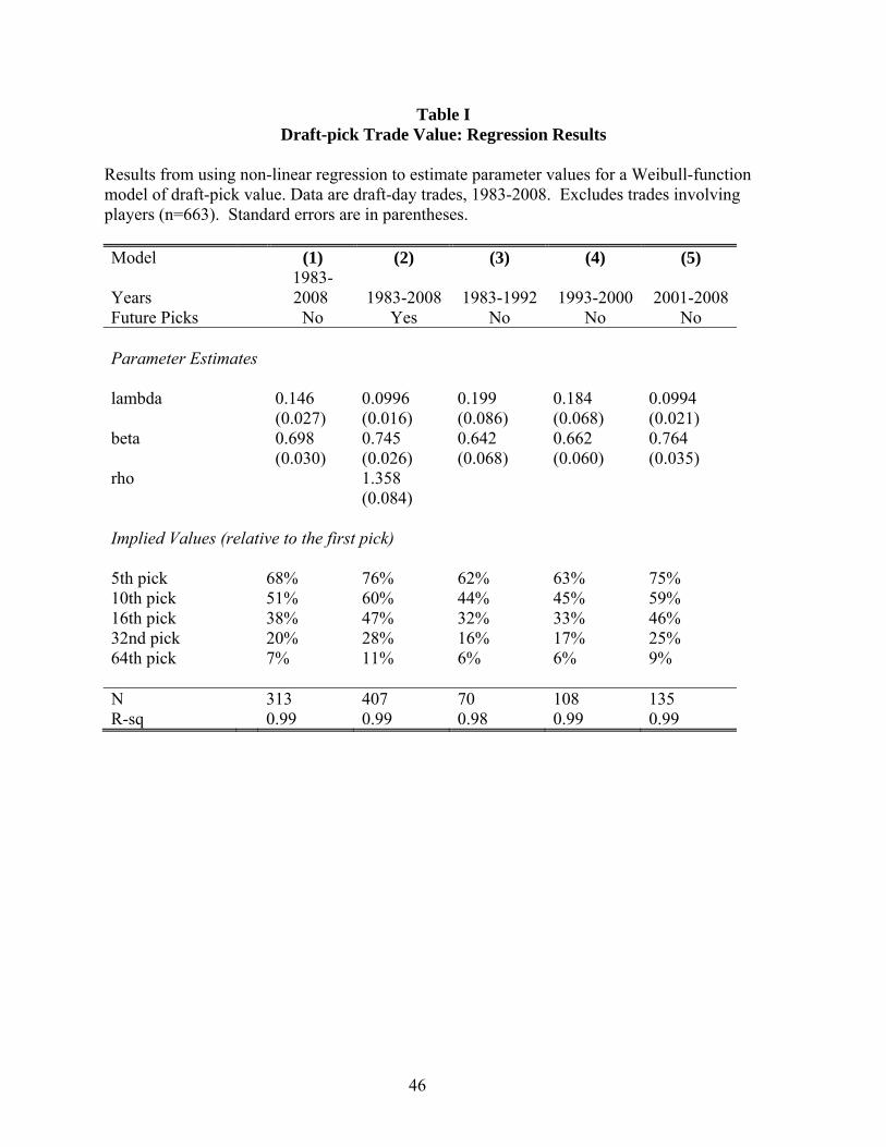
46

Table I Draft-pick Trade Value: Regression Results

Results from using non-linear regression to estimate parameter values for a Weibull-function model of draft-pick value. Data are draft-day trades, 1983-2008. Excludes trades involving players (n=663). Standard errors are in parentheses. Model (1) (2) (3) (4) (5)

Years 1983-2008 1983-2008 1983-1992 1993-2000 2001-2008

Future Picks No Yes No No No Parameter Estimates lambda 0.146 0.0996 0.199 0.184 0.0994 (0.027) (0.016) (0.086) (0.068) (0.021) beta 0.698 0.745 0.642 0.662 0.764 (0.030) (0.026) (0.068) (0.060) (0.035) rho 1.358 (0.084) Implied Values (relative to the first pick) 5th pick 68% 76% 62% 63% 75% 10th pick 51% 60% 44% 45% 59% 16th pick 38% 47% 32% 33% 46% 32nd pick 20% 28% 16% 17% 25% 64th pick 7% 11% 6% 6% 9% N 313 407 70 108 135 R-sq 0.99 0.99 0.98 0.99 0.99

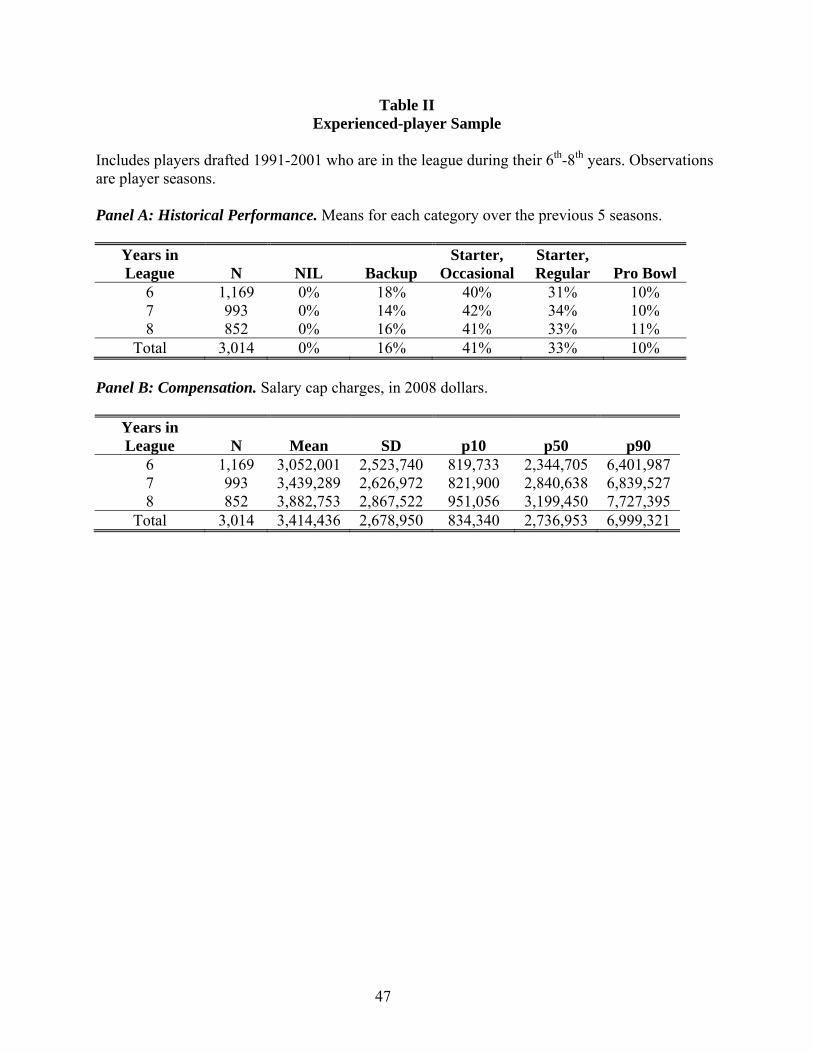
47

Table II Experienced-player Sample

Includes players drafted 1991-2001 who are in the league during their 6th-8th years. Observations are player seasons. Panel A: Historical Performance. Means for each category over the previous 5 seasons.

Years in League N NIL Backup

Starter, Occasional

Starter, Regular Pro Bowl

6 1,169 0% 18% 40% 31% 10% 7 993 0% 14% 42% 34% 10% 8 852 0% 16% 41% 33% 11%

Total 3,014 0% 16% 41% 33% 10% Panel B: Compensation. Salary cap charges, in 2008 dollars.

Years in League N Mean SD p10 p50 p90

6 1,169 3,052,001 2,523,740 819,733 2,344,705 6,401,987 7 993 3,439,289 2,626,972 821,900 2,840,638 6,839,527 8 852 3,882,753 2,867,522 951,056 3,199,450 7,727,395

Total 3,014 3,414,436 2,678,950 834,340 2,736,953 6,999,321

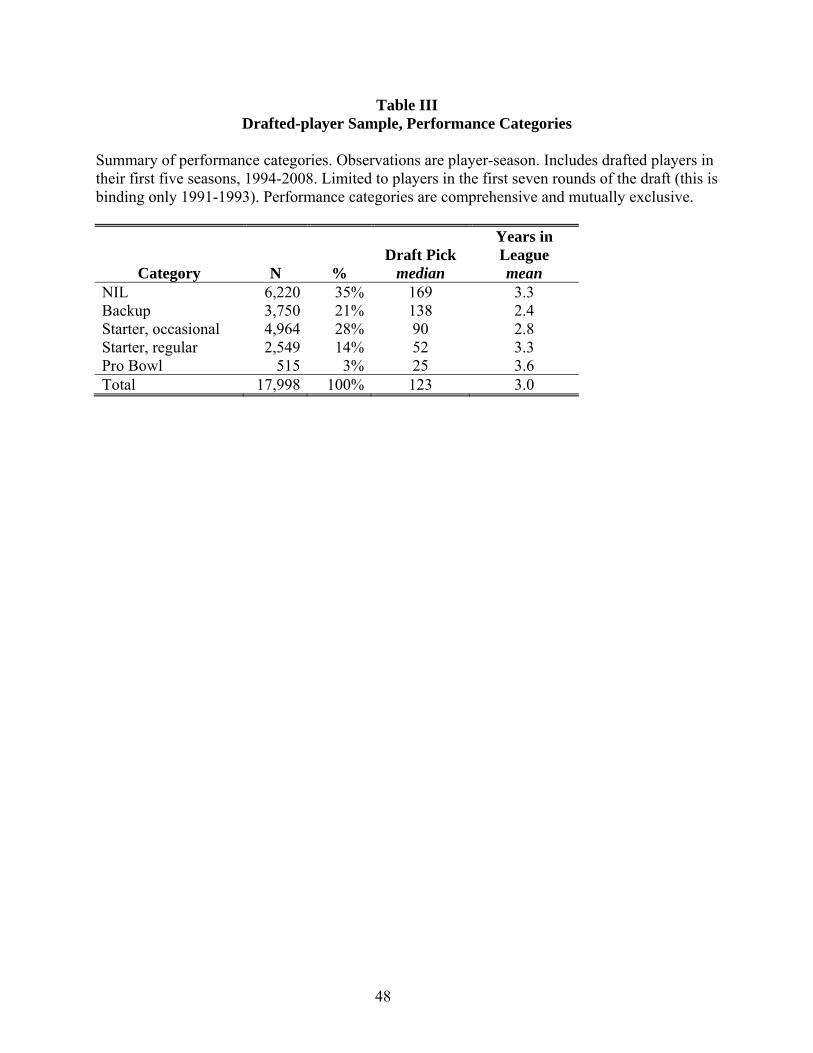
48

Table III Drafted-player Sample, Performance Categories

Summary of performance categories. Observations are player-season. Includes drafted players in their first five seasons, 1994-2008. Limited to players in the first seven rounds of the draft (this is binding only 1991-1993). Performance categories are comprehensive and mutually exclusive.

Draft Pick Years in League

Category N % median mean NIL 6,220 35% 169 3.3 Backup 3,750 21% 138 2.4 Starter, occasional 4,964 28% 90 2.8 Starter, regular 2,549 14% 52 3.3 Pro Bowl 515 3% 25 3.6 Total 17,998 100% 123 3.0

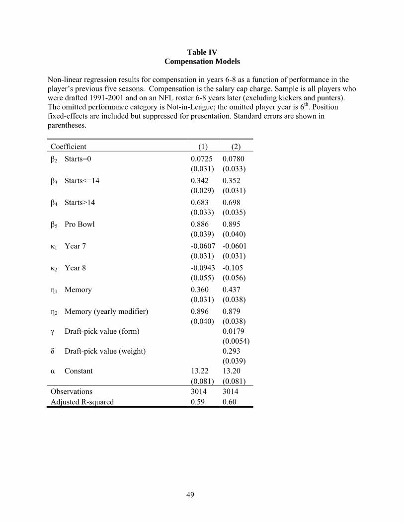
49

Table IV Compensation Models

Non-linear regression results for compensation in years 6-8 as a function of performance in the player’s previous five seasons. Compensation is the salary cap charge. Sample is all players who were drafted 1991-2001 and on an NFL roster 6-8 years later (excluding kickers and punters). The omitted performance category is Not-in-League; the omitted player year is 6th. Position fixed-effects are included but suppressed for presentation. Standard errors are shown in parentheses. Coefficient (1) (2) β2 Starts=0 0.0725 0.0780 (0.031) (0.033) β3 Starts<=14 0.342 0.352 (0.029) (0.031) β4 Starts>14 0.683 0.698 (0.033) (0.035) β5 Pro Bowl 0.886 0.895 (0.039) (0.040) κ1 Year 7 -0.0607 -0.0601 (0.031) (0.031) κ2 Year 8 -0.0943 -0.105 (0.055) (0.056) η1 Memory 0.360 0.437 (0.031) (0.038) η2 Memory (yearly modifier) 0.896 0.879 (0.040) (0.038) γ Draft-pick value (form) 0.0179 (0.0054)δ Draft-pick value (weight) 0.293 (0.039) α Constant 13.22 13.20 (0.081) (0.081) Observations 3014 3014 Adjusted R-squared 0.59 0.60

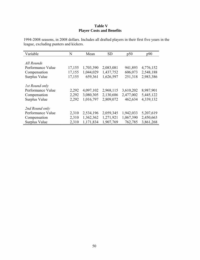
50

Table V Player Costs and Benefits

1994-2008 seasons, in 2008 dollars. Includes all drafted players in their first five years in the league, excluding punters and kickers.

Variable N Mean SD p50 p90 All Rounds Performance Value 17,155 1,703,390 2,083,081 941,893 4,776,152 Compensation 17,155 1,044,029 1,437,752 606,073 2,548,188 Surplus Value 17,155 659,361 1,626,597 251,318 2,983,386 1st Round only Performance Value 2,292 4,097,102 2,968,115 3,610,202 8,987,901 Compensation 2,292 3,080,305 2,130,686 2,477,002 5,445,122 Surplus Value 2,292 1,016,797 2,809,072 462,634 4,339,132 2nd Round only Performance Value 2,310 2,534,196 2,059,345 1,942,033 5,207,619 Compensation 2,310 1,362,362 1,271,921 1,067,390 2,450,663 Surplus Value 2,310 1,171,834 1,907,769 762,785 3,861,268

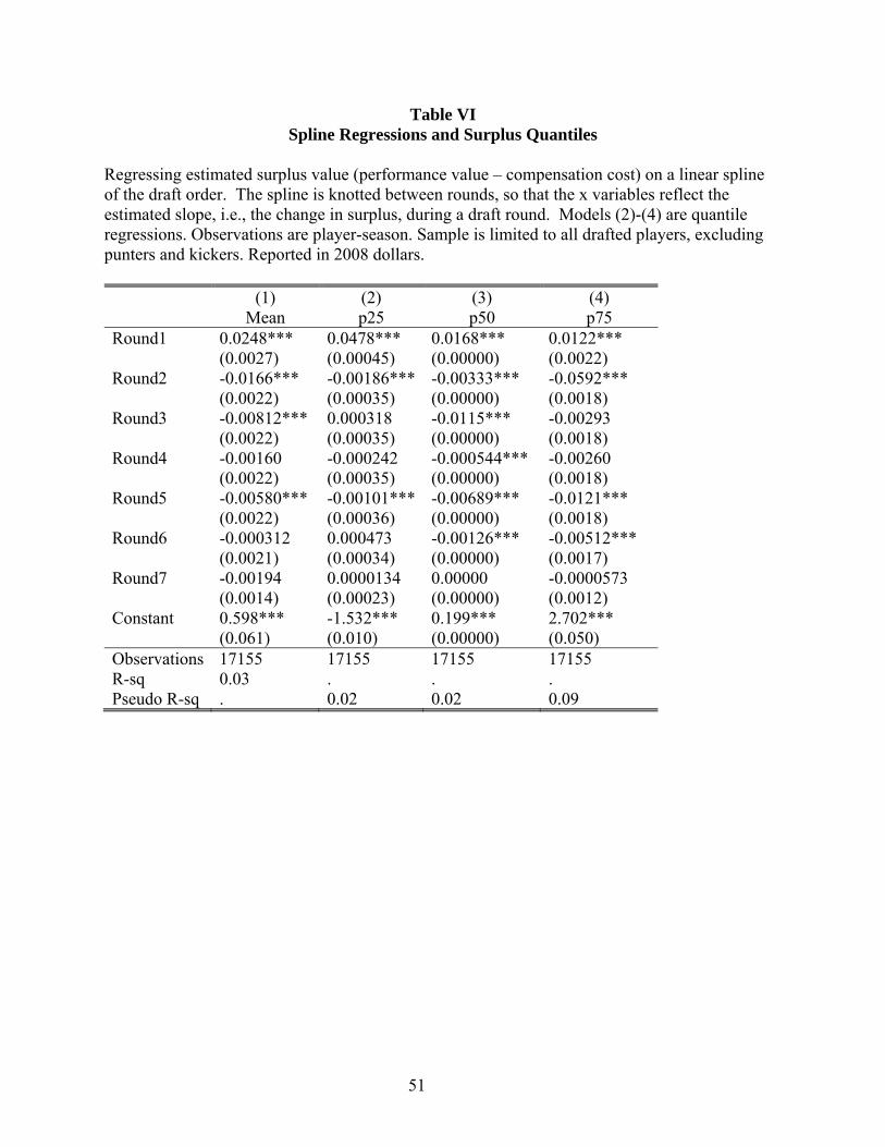
51

Table VI Spline Regressions and Surplus Quantiles

Regressing estimated surplus value (performance value – compensation cost) on a linear spline of the draft order. The spline is knotted between rounds, so that the x variables reflect the estimated slope, i.e., the change in surplus, during a draft round. Models (2)-(4) are quantile regressions. Observations are player-season. Sample is limited to all drafted players, excluding punters and kickers. Reported in 2008 dollars.

(1) (2) (3) (4) Mean p25 p50 p75 Round1 0.0248*** 0.0478*** 0.0168*** 0.0122*** (0.0027) (0.00045) (0.00000) (0.0022) Round2 -0.0166*** -0.00186*** -0.00333*** -0.0592*** (0.0022) (0.00035) (0.00000) (0.0018) Round3 -0.00812*** 0.000318 -0.0115*** -0.00293 (0.0022) (0.00035) (0.00000) (0.0018) Round4 -0.00160 -0.000242 -0.000544*** -0.00260 (0.0022) (0.00035) (0.00000) (0.0018) Round5 -0.00580*** -0.00101*** -0.00689*** -0.0121*** (0.0022) (0.00036) (0.00000) (0.0018) Round6 -0.000312 0.000473 -0.00126*** -0.00512*** (0.0021) (0.00034) (0.00000) (0.0017) Round7 -0.00194 0.0000134 0.00000 -0.0000573 (0.0014) (0.00023) (0.00000) (0.0012) Constant 0.598*** -1.532*** 0.199*** 2.702*** (0.061) (0.010) (0.00000) (0.050) Observations 17155 17155 17155 17155 R-sq 0.03 . . . Pseudo R-sq . 0.02 0.02 0.09

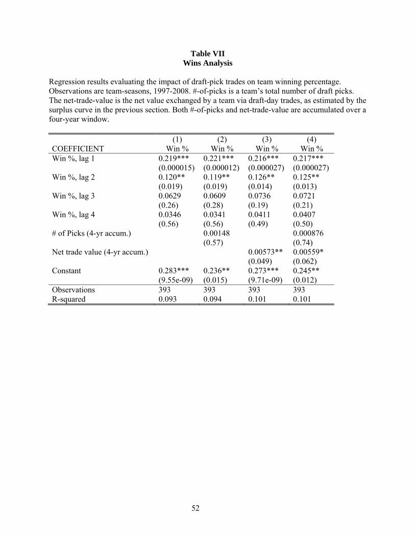
52

Table VII Wins Analysis

Regression results evaluating the impact of draft-pick trades on team winning percentage. Observations are team-seasons, 1997-2008. #-of-picks is a team’s total number of draft picks. The net-trade-value is the net value exchanged by a team via draft-day trades, as estimated by the surplus curve in the previous section. Both #-of-picks and net-trade-value are accumulated over a four-year window.

(1) (2) (3) (4) COEFFICIENT Win % Win % Win % Win % Win %, lag 1 0.219*** 0.221*** 0.216*** 0.217*** (0.000015) (0.000012) (0.000027) (0.000027) Win %, lag 2 0.120** 0.119** 0.126** 0.125** (0.019) (0.019) (0.014) (0.013) Win %, lag 3 0.0629 0.0609 0.0736 0.0721 (0.26) (0.28) (0.19) (0.21) Win %, lag 4 0.0346 0.0341 0.0411 0.0407 (0.56) (0.56) (0.49) (0.50) # of Picks (4-yr accum.) 0.00148 0.000876 (0.57) (0.74) Net trade value (4-yr accum.) 0.00573** 0.00559* (0.049) (0.062) Constant 0.283*** 0.236** 0.273*** 0.245** (9.55e-09) (0.015) (9.71e-09) (0.012) Observations 393 393 393 393 R-squared 0.093 0.094 0.101 0.101

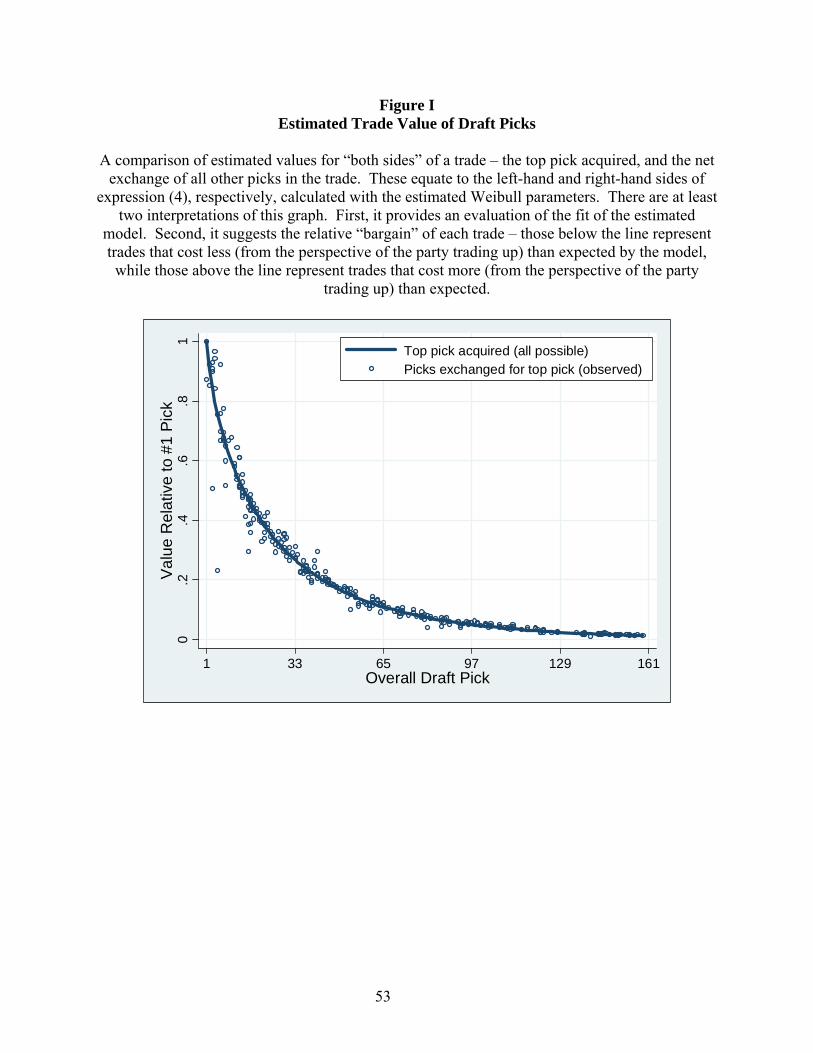
53

Figure I Estimated Trade Value of Draft Picks

A comparison of estimated values for “both sides” of a trade – the top pick acquired, and the net

exchange of all other picks in the trade. These equate to the left-hand and right-hand sides of expression (4), respectively, calculated with the estimated Weibull parameters. There are at least

two interpretations of this graph. First, it provides an evaluation of the fit of the estimated model. Second, it suggests the relative “bargain” of each trade – those below the line represent trades that cost less (from the perspective of the party trading up) than expected by the model, while those above the line represent trades that cost more (from the perspective of the party

trading up) than expected.

0.2

.4.6

.81

Valu

e R

elat

ive

to #

1 Pi

ck

1 33 65 97 129 161Overall Draft Pick

Top pick acquired (all possible)Picks exchanged for top pick (observed)

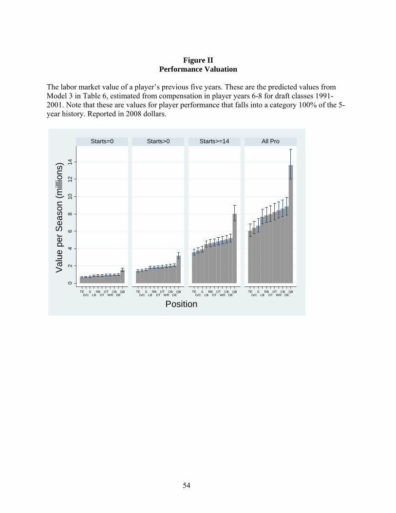
54

Figure II

Performance Valuation

The labor market value of a player’s previous five years. These are the predicted values from Model 3 in Table 6, estimated from compensation in player years 6-8 for draft classes 1991-2001. Note that these are values for player performance that falls into a category 100% of the 5-year history. Reported in 2008 dollars.

02

46

810

1214

TEG/C

SLB

RBDT

OTWR

CBDE

QB TEG/C

SLB

RBDT

OTWR

CBDE

QB TEG/C

SLB

RBDT

OTWR

CBDE

QB TEG/C

SLB

RBDT

OTWR

CBDE

QB

Starts=0 Starts>0 Starts>=14 All Pro

Val

ue p

er S

easo

n (m

illio

ns)

Position

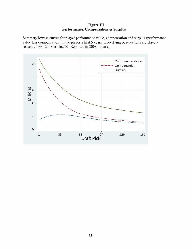
55

Figure III Performance, Compensation & Surplus

Summary lowess curves for player performance value, compensation and surplus (performance value less compensation) in the player’s first 5 years. Underlying observations are player-seasons, 1994-2008. n=16,502. Reported in 2008 dollars.

01

23

45

Mill

ions

1 33 65 97 129 161Draft Pick

Performance ValueCompensationSurplus

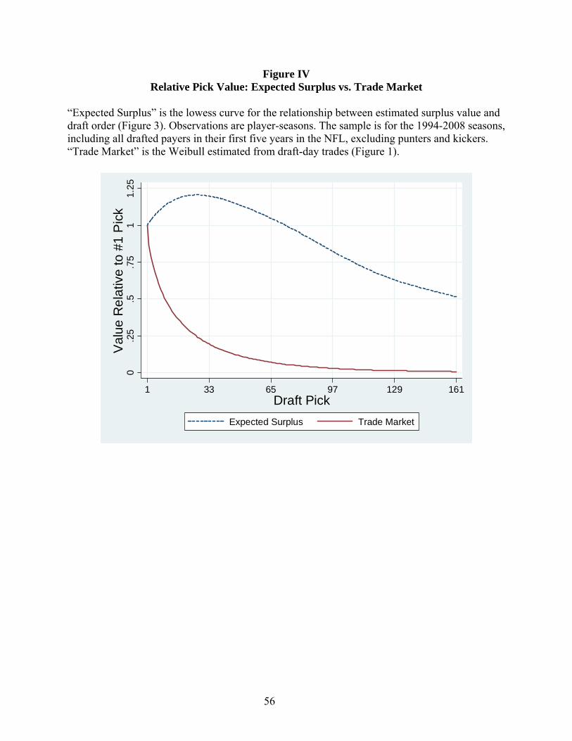
56

Figure IV Relative Pick Value: Expected Surplus vs. Trade Market

“Expected Surplus” is the lowess curve for the relationship between estimated surplus value and draft order (Figure 3). Observations are player-seasons. The sample is for the 1994-2008 seasons, including all drafted payers in their first five years in the NFL, excluding punters and kickers. “Trade Market” is the Weibull estimated from draft-day trades (Figure 1).

0.2

5.5

.75

11.

25V

alue

Rel

ativ

e to

#1

Pic

k

1 33 65 97 129 161Draft Pick

Expected Surplus Trade Market

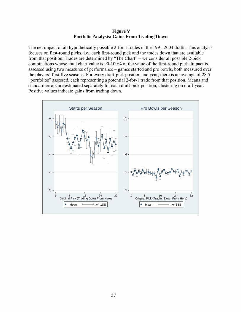
57

Figure V Portfolio Analysis: Gains From Trading Down

The net impact of all hypothetically possible 2-for-1 trades in the 1991-2004 drafts. This analysis focuses on first-round picks, i.e., each first-round pick and the trades down that are available from that position. Trades are determined by “The Chart” – we consider all possible 2-pick combinations whose total chart value is 90-100% of the value of the first-round pick. Impact is assessed using two measures of performance – games started and pro bowls, both measured over the players’ first five seasons. For every draft-pick position and year, there is an average of 28.5 “portfolios” assessed, each representing a potential 2-for-1 trade from that position. Means and standard errors are estimated separately for each draft-pick position, clustering on draft-year. Positive values indicate gains from trading down.

-30

36

9

1 8 16 24 32Original Pick (Trading Down From Here)

Mean +/- 1SE

Starts per Season

-.50

.51

1.5

1 8 16 24 32Original Pick (Trading Down From Here)

Mean +/- 1SE

Pro Bowls per Season

the loser's curse: decision making and market efficiency

Documents