1

The Macro Impact of Microfinance in Bangladesh:

A CGE Analysis

Selim Raihan, S. R. Osmani and M. A. Baqui Khalily*

I. INTRODUCTION

Much has been written on the impact of microfinance on the welfare of borrowers, but not

much is known about its impact on the economy as a whole.1 In the early days of microfinance,

when its reach was limited, the relative neglect of its macro impact was understandable. But

with rapid expansion of microfinance, this issue has become increasingly relevant. This is

especially true for Bangladesh, where microfinance penetration has been the strongest in the

world, covering more than half of the rural population and increasing proportion of urban

population as well. According to a recent study, some 55 percent of rural households have taken

microfinance at some stage in their lives, and almost 46 percent hold the status of current

borrowers (as of 2010).2 With such huge expansion, microfinance is bound to have direct and

indirect repercussion on the overall economy. The present study makes a pioneering attempt to

assess the macroeconomic impact of this expansion – in particular, to estimate the contribution

of microfinance to the national income of Bangladesh, as measured by its gross domestic

product (GDP), by using a static computable general equilibrium (CGE) model.3

A considerable amount of scholarly effort has been expended in the last couple of decades to

evaluate the impact of microfinance on the welfare of the borrowers – as measured by economic

indicators such as income, consumption and poverty as well as a host of non-economic

indicators such as health, education, and women’s empowerment. While this literature has at

times been riven by heated controversies, the overall conclusion that microfinance has

improved borrowers’ welfare remains valid – especially in Bangladesh, where borrowers had

a much longer exposure to it than anywhere else in the world.4

Not much is known, however, about the macro-level impact of microfinance. The motivation

for the present paper stems from the recognition that if the macro impact of microfinance is to

be significantly visible in any country, it must be in Bangladesh because of the manner in which

the size and structure of the microfinance sector has undergone some radical transformation in

recent years.

* The authors gratefully acknowledge many helpful comments and suggestions received from Shamsul Alam,

Quazi Kholiquzzaman Ahmed, Quazi Mesbahuddin Ahmad, Mustafa K. Mujeri, Sultan H. Rahman, two

anonymous referees and the editor of this journal. The usual disclaimer applies. 1 The term microfinance has a broader connotation than microcredit in so far as it also includes savings and

insurance in addition to credit, although credit is by far the biggest component of microfinance almost everywhere,

including Bangladesh. 2 See Osmani et al. (2015). This study was based on a nationally representative household survey covering the

whole or rural Bangladesh and was carried out in 2010 by the Institute of Microfinance in Dhaka. 3 Although the paper is related to Bangladesh, the methodology adopted for the purpose of estimating the macro

impact of microfinance may be applicable in other countries as well, with suitable modifications in light of

country-specific features of both the microfinance sector and the economy in question. It should be noted,

however, that the magnitude of the impact that might be found in other countries may not be as large as we have

found for Bangladesh for the simple reason that in no other country has the reach of microfinance extended as far

as it has in Bangladesh. 4 See, for example, Mahmud and Osmani (2016) who arrive at this conclusion after an extensive review of the

relevant evidence.

2

2

This transformation includes the following features: (i) microfinance has expanded enormously

in both scope and scale in Bangladesh, covering more than half of the rural population; (ii)

almost one third of the microcredit is invested in micro enterprises creating full-time

employment opportunities for some 10 million individuals; (iii) increasingly, larger loan sizes

are being offered by the Microfinance Institutions (MFIs) to the more enterprising borrowers;

(iv) microcredit is invested in diversified activities including non-financial activities; and (v)

non-financial services like training and education have increasing presence in microfinance

program design in Bangladesh.

These transformations have had a profound impact on the lives of the poor. Longitudinal

studies in Bangladesh show that microfinance has contributed to (i) creating substantial amount

of full time employment; (ii) increasing the intensity of financial inclusion; (iii) improved

productivity in microenterprises, (iv) accumulation of assets, and (v) sustained reduction in

poverty, especially for those who have had a long exposure to microfinance.5

When an intervention positively affects the economic lives of close to half of a country’s

population, there is a good a priori reason to believe that it will have a positive effect on the

overall economy as well. However, the magnitude of the macroeconomic impact cannot be

obtained simply by aggregating the impact on borrowers because the intervention also has

direct and indirect repercussion on the rest of the economy, many of which would be positive

but some could be negative as well. It is necessary to adopt a general equilibrium approach in

order to capture these diverse effects on the overall economy encompassing both borrowers

and non-borrowers, as distinct from the partial equilibrium approach that underlies the

evaluation of the direct impact on borrowers’ welfare. This is the approach the present paper

adopts.

A useful vantage point from which to adopt a general equilibrium approach to the macro effect

of microfinance is the concept of financial development, because expansion of microfinance

constitutes an important dimension of overall financial development of an economy. There

exists a burgeoning literature on both the theory and empirics on how financial development

affects the real economy through a variety of channels.6 The present paper captures a number

of such channels through which microfinance has affected the GDP of Bangladesh – viz.,

capital accumulation, productivity improvement, and reallocation of labor and capital across

sectors. For this purpose, the study uses a CGE model based on an updated version of the Social

Accounting Matrix (SAM) of Bangladesh with the base year of 2012.7 The model is simulated

to derive a measure of GDP that would have obtained in Bangladesh in the counterfactual

scenario in which there were no microfinance at all. The difference between this counterfactual

GDP and the actual GDP is taken as the contribution of microfinance to GDP. Our estimates

suggest that microfinance has contributed somewhere in the range of 9-12 percent to the GDP

of Bangladesh. As pointed out in the concluding section, however, partly because of data

5 The relevant evidence is discussed in section II below. 6 See Pagano (1993) for an illuminating discussion of the channels through which financial development can affect

the real economy. See also Masudova (2010) for discussion of the transmission channels in the context of

microfinance. 7 Conventionally, SAM refers to a single representative year (a year of normal representative economic activities

and free from any major external and internal shocks), providing a picture of the structure of the economy. The

reason for using 2012 as the reference year for the present study is that it is the latest year for which a SAM is

available for the Bangladesh economy. But it should be noted that the broad conclusions of the study do not apply

to that particular year alone. Since 2012 is representative of a ‘normal’ year in Bangladesh, the results of the paper

can be seen as reflecting the macro effects of microfinance in Bangladesh in recent years.

3

3

limitations and partly because of the exploratory nature of the present exercise, it was not

possible to incorporate a number of transmission mechanisms that could potentially affect

national income – some positively and some negatively. A further limitation stems from the

static nature of the CGE model that has been used in the paper; while a static model is useful

for an exploratory exercise, a dynamic model is needed to fully capture the longer-term impacts

of microfinance. Future research could be fruitfully directed towards addressing these

limitations.

The rest of the paper is organized as follows. Section II provides an overview of the

microfinance sector in Bangladesh so as to set the context in which the modeling exercise has

been undertaken later in the paper. Section III offers an analytical review of the existing

literature on the macroeconomic impact of microfinance with a view to extracting some lessons

for our own modelling exercise. Section IV explains the methodology and modelling

assumptions adopted in this study. Section V presents the results; and finally, some concluding

remarks are offered in section VI.

II. OVERVIEW OF THE MICROFINANCE PROGRAM IN BANGLADESH

The microfinance sector in Bangladesh has undergone some major transformations over the

past two decades. MFIs started as non-government voluntary social organizations with the

basic objective of providing microfinance services to poor households. The most well-known

of them, the Grameen Bank, started formally in 1983 under the Grameen Bank Ordinance.

According to the latest available statistics, some 740 MFIs are operating with a network of

around 19,000 branches, employing over 250,000 people and serving over 34 million

borrowers (CDF, 2014).

Although Bangladesh has a long history of microfinance dating back to 1978, the sector

essentially took off in 1992 with the establishment of Palli Karma Sahayak Foundation

(PKSF), which acts as a wholesale provider of funds to the MFIs (Faruqee and Badruddoza,

2012). Since microfinance services are provided in a manner that minimizes the risk of default

despite the absence of collateral, increasingly a number of commercial banks have also

ventured to come forward to finance microfinance operations through wholesale lending to

MFIs. These banks are now an important provider of external fund. However, member savings

and reserves (generated out of surplus) remain the major source of financing of the total assets

held by the MFIs.8

From the very inception of the microfinance sector in Bangladesh, access to both savings and

credit has been recognized as essential pre-requisites for alleviating poverty. In order to

enhance the savings rate, the act of saving was invariably linked with micro lending. The

original Grameen Bank model introduced compulsory weekly savings as a precondition for

access to microcredit (Khandker, 1998). Following the devastating flood of 1988 and 1998,

flexible savings schemes were introduced. Other large MFIs, such as BRAC9, have also

emphasized savings. The greater emphasis on member savings was based on the notion that

access to own savings will reduce dependency on microcredit.

8 For more on the structure and evolution of the microfinance sector in Bangladesh, see chapters 2 and 3 of

Mahmud and Osmani (2016). 9 BRAC was established in 1972 as the “Bangladesh Rehabilitation Assistance Committee”. Later the name was

changed to “Bangladesh Rural Advancement Committee” keeping the acronym unchanged. Currently, however,

the name BRAC stands for itself, rather than as an acronym.

4

4

All the MFIs have followed essentially the same ‘microfinance’ model, with some minor

variations. However, with the increase in loan size and volume of loans, many MFIs have begun

to introduce micro insurance schemes, especially since 2000. As a result, the microfinance

model currently contains all three essential elements of finance – namely, credit, savings and

insurance.

The MFIs operate in almost all parts of the country with the exception of some inaccessible

areas. Table 1 shows the outreach of MFIs operating in Bangladesh over the period 1996-2014.

A structural change has occurred, in terms of growth of outreach, at around 2006. Since that

year, the sector has experienced exponential growth in terms of membership mobilized, annual

loans disbursed, loans outstanding and net savings. Membership increased rapidly since 2006,

reaching the figure of 34 million by 2014. Compared to the period 1996-2000, average annual

number of members during the period 2011-14 was 3 times higher. During the same period,

average annual loans disbursement increased by almost 15 times and average net savings by

17 times.

The increase in savings mobilization has drastically reduced MFIs’ dependency on external

finance; by the end of 2014, net savings constituted 55 percent of loans outstanding. It has also

strengthened the capability of borrowing households to invest in productive activities, and has

better equipped them to cope with shocks.10

Table 1: Average Outreach of MFIs, 1996-2014 (taka in million)

Period Number of

Members

Annual

Disbursement

Loans

Outstanding

Net Savings

1996-2000 10,974,659 36,533 24,387 11,163

2001-2005 18,595,932 84,810 55,234 33,335

2006-2010 33,004,304 290,973 155,422 108,031

2011-2014 32,839,003 538,112 337,220 190,997

Source: Credit Development Forum (CDF), Bangladesh Microfinance Statistics (various years)

A growing body of evidence shows that increased access to credit and savings has had a

positive impact on poverty alleviation, income, and return on investment.11 By using long-term

panel data, Khandker et al. (2016) have recently shown that with access to credit alone, some

2.5 million households graduated sustainably from poverty by the end of 2010. With increasing

loan size and access to non-financial services offered by the MFIs, the number of graduating

households and the rate of poverty reduction would be even higher. This is demonstrated in

Osmani et al. (2015), which shows that by sustainably improving the wealth level of borrowers

microfinance has contributed to 29 percent reduction in poverty. Khalily et al. (2014) have

shown that households with access to credit and non-financial interventions like training and

health services had higher rate of graduation from extreme poverty than the counterfactual

groups with access to microfinance alone in areas chronically affected by seasonal hunger.

It is instructive to note that all of the recent studies mentioned above reveal a much higher level

of impact of microfinance on poverty reduction compared to the studies prior to 2010 (which

10 A recent study has found that households with access to savings have higher probability of being out of poverty

(Khalily et al., 2015). 11 There are some critical studies questioning the positive findings of early papers on the impact of microfinance

in Bangladesh. But as discussed in section III below, and explained more fully in Mahmud and Osmani (2016,

chapter 7), most of these critiques lack credibility, especially in the light of more recent studies. Hence we mention

only the more recent studies in this section.

5

5

include, for example, Zohir et al., 2001; Rahman et al., 2005; Khandker, 1998). The reasons

for the bigger impact found in more recent studies can be traced to some of the transformations

that have occurred in the microfinance sector in recent years. These transformations relate to

rising loan size, changing loan use pattern, and provision of non-financial services, among

others.

(a) Loan size: The emergence of Microcredit Regulatory Authority (MRA) in 2006 has changed

the structure of the microfinance market in a significant way. While more active regulation has

imposed a cost on the licensed MFIs, on the positive side the MRA has allowed them to lend

as high as 50 percent of the loanable fund. This has enabled the MFIs to offer larger-sized loans

for micro enterprises. For example, in 2014, as much as 28 percent of the loans disbursed were

accounted for by micro enterprises. Although one may argue about this might indicate possible

drifting of the MFIs from their social mission of poverty alleviation, financing micro

enterprises has been linked to inclusive economic growth – in particular, creation of new

employment opportunities. Muneer and Khalily (2015) showed that these enterprises generated

average economic returns of 64 percent, and created around two full time employments per

micro enterprise. They further showed that it has also had a positive impact on total factor

productivity (TFP).12 Considering the number of micro enterprises and income generating

activities of microcredit borrowers, it has been estimated that some 10 million new

employments have been created in Bangladesh.

(b) Loan use: Loans that are offered by MFIs are utilized by borrowers for multiple purposes.

Because of the fungibility of funds, it is very difficult to trace the actual use of borrowed funds.

Nevertheless, careful estimates of actual uses made by households (as distinct from declared

uses recorded in MFIs’ books) have recently been made using detailed surveys of loan use.

Based on two separate nationally representative household-hold surveys, it has been estimated

by Osmani et al. (2015) and Khalily et al. (2015) that some 47-48 percent of microcredit is

currently used for productive purposes. In the early stage of microfinance development in

Bangladesh, by far the major part of the microcredit was used for off-farm economic

enterprises, with very little of it going to agriculture. This has changed dramatically in the

recent years. During the past three years (2012-14), more than 25 percent of the loans were

used for agriculture – most of it for crop cultivation.

(c) Non-financial services: It is widely recognized that microfinance alone cannot eliminate

poverty because of the existence of deep-rooted structural poverty. A multi-pronged strategy

is required involving education, housing and wealth accumulation, among others. A small

amount of credit may be a step towards poverty alleviation, but the impact of microfinance is

magnified when the borrowers have necessary skills to utilize it. In recognition of this

complementarity between finance and skills, provision of relevant training has become an

increasingly important feature of the microfinance sector in Bangladesh. Although data is not

available for all years on the number of members receiving training, recent statistics show that,

on an average, every year more than two percent of the members received training, more than

25 percent of which was related to livestock and poultry (CDF, 2014). Not all the MFIs are,

however, engaged in providing training because of the lack of appropriate infrastructure and

low level of operations. Nonetheless, more than half of the MFIs provide training to their

clients. It is plausible to argue that increased provision of training has raised the potency of

microfinance in enhancing its impact on borrowers’ income. This is evident from Khalily et al.

12 Similar results were also reported by Osmani et al. (2015), Khalily and Khaleque (2013) and Khandker et al.

(2013).

6

6

(2014) who showed that microfinance combined with non-financial interventions like training

have contributed 15 percent more income compared to pure microfinance without any training

in the relevant areas of investment.

Because of the multi-dimensionality of poverty, anti-poverty interventions will also require

interventions for social or community development, which will empower participating poor

households, and ensure access to different socio-economic institutions. Bearing this in mind,

more than 74 percent of the MFIs are engaged in social development programs with major

focus on education and related supports, water and sanitation, health and treatment, women’s

empowerment and development in general (CDF, 2014).

All the elements of the transformation of the microfinance sector described above have had a

positive impact on the livelihoods of the borrowers. First, access to non-financial services has

reduced vulnerability of the households and enabled them to earn higher income from their

investments on a sustained basis. Second, higher average loan size has enabled households to

invest in microenterprises, with higher returns. Third, increasing presence of micro insurance

has helped reduce adverse impact of negative shocks. Fourth, creation of multiple income

sources through use of credit, savings and occupational trainings has helped raise the level of

household income. The present study seeks to estimate the magnitude of these impacts at the

aggregate level by measuring the impact on national income.

III. REVIEW OF LITERATURE ON THE MACROECONOMICS OF

MICROFINANCE

Before considering the macroeconomic effect of microfinance, it is worth noting that if the

reach of microfinance is extensive and if it is found to improve the economic condition of the

average borrower, it would be reasonable to argue that the macroeconomic impact cannot but

be positive. The existing vast literature on the microeconomic impact of microfinance on

borrowers’ welfare is, therefore, relevant in the macroeconomic context as well. As is well

known, however, this literature has been rife with controversies. The pioneering studies such

as Pitt and Khandker (1998), which claimed to show through careful econometric analysis that

microfinance exerted a positive impact on borrowers’ welfare, were subsequently subjected to

severe criticism on methodological grounds (e.g., Roodman and Morduch, 2014). The critical

view was further strengthened by a spate of studies that claimed that once the effects of other

factors were effectively controlled for with the help of randomized controlled trials (RCTs),

microfinance appeared to have very little impact on borrowers’ economic condition.13 The

intellectual impact of these critical studies has been quite strong, resulting in skepticism in

some quarters regarding the efficacy of microfinance as a tool for poverty reduction.

More recent research has shown, however, that this skepticism is unwarranted, for a number of

reasons.14 First, the critical studies which took issue with the early findings of positive impact

on methodological grounds were themselves methodologically flawed. Second, the RCT-based

studies, which were otherwise methodologically sound, had the inherent limitation that they

could observe the impact only over a short period of time, whereas both commonsense and

empirical evidence suggest that it is only after a prolonged exposure to microcredit that poor

people can begin to capture appreciable economic benefits from it. Third, several recent studies,

13 The findings of these studies are summarised in Banerjee (2013) and IPA (2015). It should be noted that none

of these studies was related to Bangladesh. 14 Mahmud and Osmani (2016, chapter 7) provides an extensive review of this research.

7

7

which avoid the early methodological criticisms by using panel and quasi-panel data as

opposed to cross-section data, demonstrate quite conclusively that prolonged exposure to

microfinance makes significantly positive contribution to the economic lives of the poor.

These empirical findings are in line with a simulation exercise carried out by Rashid et al.

(2011) using the framework of agent-based modeling (ABM). The study simulated a large

number of alternative scenarios through parametric variation of agent’s behavior and the

circumstances in which they operate. In all of the simulations, the average wealth level of the

poor was found to decline for a while, because it takes time to make products, engage in trade

and then gain the fruits of microenterprise; but after a certain period of time the wealth of the

poor begins to increase and maintains a higher rate of increase.

It is sometimes contended that even if microfinance is helping the poor now, there is a danger

that this would no longer be the case as the scale and reach of microfinance expand, because

such expansion will allegedly lead to over-indebtedness, rising defaults and hence higher

interest rates. Lahkar and Pingali (2016) have shown, however, that this apprehension too may

be unwarranted. Using a standard screening model, they show that, even if expansion of

microfinance leads to higher interest rates, screening effects will lead to higher borrower

welfare. This will happen because, firstly, all borrowers previously denied credit would be able

to obtain loans, and, secondly, screening costs for pre-existing borrowers will go down.

There is thus a strong empirical basis for the claim that microfinance has had a positive effect

on borrowers’ welfare. And if these borrowers happen to constitute a large percentage of the

population, as is the case in Bangladesh, one should expect the macro effect to be positive as

well. Of course, the magnitude of the macro effect cannot be deduced simply by aggregating

individual welfares of borrowers because of the presence of general equilibrium effects on the

overall economy. In the end, the macro effect must be deduced from a macro-analytical

perspective.

One such perspective is to view the expansion of microfinance as part of the process of financial

development of an economy. From this perspective, there is a simple intuitive reason for taking

the view that microfinance should in principle make a positive contribution towards the growth

of national income. Theoretical research as well as a growing body of empirical evidence lends

strong support to the view that financial development exerts a positive impact on economic

growth.15 By reducing the costs of information, enforcement and transaction, a well-

functioning financial system promotes growth through a number of channels: viz., savings

mobilization, provision of investment information, better monitoring/governance, risk

management, and facilitation of exchange of goods and services.

In the context of financial development of Bangladesh, the positive savings effect was found

by Sahoo and Das (2013) and more direct evidence on the positive effect on growth and poverty

reduction was found by Uddin et al. (2014). In general, however, empirical studies on the

relationship between financial development and growth have sometimes come up with

conflicting evidence; while the vast majority of studies have found a positive effect, some have

found little effect and a few have found even a negative effect. Such diversity of results can

arise from (a) non-linearity (in particular, the presence of threshold effects) in the relationship

between financial development on economic growth – as modeled, for example, in Eggoh and

Villieu (2014) and (b) from the fact that the impact of financial development on growth depends

15 For a comprehensive review of the relevant theory and evidence, see Levine (2005).

8

8

on various other factors – such as the level of development, degree of openness of an economy,

and the size of the government, as found by Herwartz and Walle (2014). In fact, it is entirely

possible that there is an optimal level of financial development corresponding to the level of

overall economic development, and excessive financial development, relative to the optimal,

may be just as harmful as less than optimal development (Bhattarai, 2015).

None of this, however, detracts from the central message that financial development does in

general promote economic growth, other things remaining the same. Since the spread of

microfinance contributes to the process of overall financial development by correcting a market

failure at the lower end of the financial market, it stands to reason that growth of microfinance

should also facilitate economic growth.

The same conclusion emerges directly from some recent evidence related specifically to the

macro impact of microfinance. This literature recognizes that one of the problems in empirical

testing of the relationship between microfinance (and finance in general) and economic growth

is that causality can run both ways: just as the spread of microfinance can affect growth, there

can also be a reverse causation from growth to the spread of microfinance.16 The statistical

methodologies employed to study the impact of microfinance on growth must be nuanced

enough to be able to isolate the true effect of microfinance from the vitiating effect of reverse

causation. The study by Masudova (2010) tried to do precisely that by employing the Granger

causality test. Applying this test to cross-country data from 102 countries she found evidence

that greater spread of microfinance helps achieve faster economic growth, although the strength

of the impact depends (positively) on the underlying level of development of the economy. A

more recent study applied the generalized method of moment to isolate out the effect of reverse

causation, and found evidence for the growth-promoting effect of microfinance in a sample of

71 developing countries (Donou-Adonsou and Sylwester, 2015).

Despite such support from both theory and evidence, some critics of microfinance continue to

remain highly skeptical about the growth-enhancing effect of microfinance. In fact, critics such

as Bateman and Chang (2009) go so far as to suggest that while bringing a measure of short

term relief to some of the poor people, microfinance may eventually prove to be a barrier to

long-term sustainable development. Their argument seems to rest on two premises. First, the

enterprises supported by microfinance (to the extent that microfinance supports enterprises at

all rather than being diverted to unproductive uses) are inherently less efficient than larger

enterprises supported by the mainstream financial market owing to the absence of scale

economies and other reasons. Second, spread of microfinance is tantamount to diversion of

funds from mainstream finance. Together, these two premises lead to the conclusion that spread

of microfinance leads to less efficient use of resources overall and thus stymies economic

growth. No evidence is adduced, however, to support either of the premises. In fact, the second

premise is completely at odds with the current reality of the microfinance sector in Bangladesh

in which, as noted in section II, some 55 percent of outstanding loans are financed from within

the sector itself – i.e., from the borrowers’ savings and only 28 percent of loans outstanding is

financed by external borrowing from banking sector.17

In contrast to the outlandish claims made by critics such as Bateman and Chang, a much more

nuanced point has recently been made by a number of theoretical studies on the

macroeconomics of microfinance. These studies have made a fairly compelling case for

16 For evidence on the existence of reverse causation, see Ahlin et al. (2011). 17 In the case of Grameen Bank, the largest MFI in Bangladesh, internal savings in fact exceeds the amount of

loan outstanding.

9

9

recognizing that in theory at least there may exist some channels through which microfinance

may exert a negative effect on growth. The import of these studies is not to assert that

microfinance will necessarily act as an impediment to growth but to alert us to the fact that

there are multiple channels through which microfinance can affect growth and while some of

those channels may transmit a positive impact (for example, those emphasized by the standard

literature on finance and growth) some others may act as a conduit of negative impact. In so

far as the negative channels operate in a particular empirical context, the potentially positive

impact of microfinance may be attenuated to some extent, and may in extreme cases be

completely offset.

An example of studies in this vein is that of Emerson and McGough (2010), which examines

the impact of microfinance on growth via investment in human capital. In the standard

literature, it is common to assume that by ensuring greater access to finance at reasonable cost,

microfinance would enable poor households to spend more on the schooling of children,

thereby contributing to the growth of human capital, which in turn would promote growth.18

The study by Emerson and McGough, however, highlights the existence of a mechanism that

may subvert this positive impact. Their argument is based on the premise that by raising the

returns to household-based enterprises microfinance will also raise the opportunity cost of

schooling. This will have the effect of discouraging parents from sending children to the school,

even as greater access to credit encourages them to do so. Two conflicting forces would thus

be in operation. The net effect is ambiguous. However, by building on models of household

decision-making in the presence of microfinance, as developed by Wydick (1999) and

Maldonadoa and González-Vega (2008), the authors show that there exists a range of

microfinance amounts that would result in a net reduction of schooling, especially given the

manner in which microfinance currently operates by demanding early and frequent repayment.

The authors then postulate the existence of externalities in education to argue that even though

the decision to reduce schooling may be beneficial for the borrowing households themselves,

it might hurt overall economic growth.19

The idea of conflicting effects operating through alternative channels is a recurring theme in

other studies of this genre. An early example is the study by Ahlin and Jiang (2008), who

examined the long-run effects of microfinance on development in an occupational choice

model similar to that of Banerjee and Newman (1993). A crucial feature of this model is the

distinction between self-employment and entrepreneurship. Assuming that entrepreneurship is

more efficient than self-employment, the model postulates a hierarchy of three occupations

characterized by three distinct technologies ranked by productivity and scale; in ascending

order, they are subsistence, self-employment, and entrepreneurship. Given this framework,

microfinance’s contribution to national income would depend on the rate at which it enables

the labor force to move up the occupational-cum-technological scale. The study asserts that

given the nature of microfinance as it currently operates, its positive impact derives almost

entirely from the graduation from subsistence to self-employment but hardly anything at all

from the potentially much more productive graduation from self-employment to

entrepreneurship. In fact, the model even allows for the possibility of a negative effect on the

latter account when general equilibrium effects are considered. The negative effect can arise

because of the impact on the wage rate. As the labor force moves from subsistence to self-

18 A whole genre of theories linking income distribution with growth has been developed in the last couple of

decades based on this presumed relationship between access to credit and human capital formation. For an

excellent review of the literature, see Voitchovsky (2009). 19 Although conceptually possible, the empirical relevance of this argument would be limited in Bangladesh,

where primary and secondary education is free and also education of children is one of the core goals of MFIs.

10

10

employment, the wage rate would rise because of the reduction of labor supply in the market

for wage labor. Higher wage rate in turn may reduce entrepreneurial profits and thereby cause

attrition of unsuccessful entrepreneurs from the entrepreneurial class. This will have a negative

effect on growth, which in extreme cases may even swamp the positive effect emanating from

the transition from subsistence to self-employment.

The general equilibrium effect operating via the labor market is also the key for the study by

Buera et al. (2012), who gave a quantitative assessment of both aggregative and distributional

effect of microfinance focused on small businesses. They employed a general equilibrium

model to capture the indirect effects of microfinance operating via the wage rate and used some

empirical parameters drawn from the experience of microfinance in developing countries in

order to derive their quantitative estimates. Conceptually, the impact of microfinance on

national income can be decomposed into two routes – namely, impacts on TFP and capital

accumulation. The study finds that the two routes can affect national income in opposite

directions: the impact on TFP makes a positive contribution to GDP while the impact on capital

accumulation makes a negative contribution. TFP rises by 4 percent, with the majority of the

gain coming from a more efficient distribution of capital among entrepreneurs. At the same

time, however, by inducing higher wages microfinance redistributes wealth from higher-ability

entrepreneurs with higher saving rates to lower-productivity individuals with lower saving

rates. As a result, aggregate saving rates fall, bringing down aggregate capital by 6 percent.

This offsets most of the increase in TFP, and output increases by less than 2 percent. In short,

the positive impact of the increase in TFP is counterbalanced in part by lower capital

accumulation resulting from the redistribution of income from high-savers to low-savers.

Nevertheless, the vast majority of the population is positively affected through the increase in

equilibrium wages. As a result, the redistributive impact of microfinance is found to be much

stronger than its aggregative impact.

Thus, as in the model of Ahlin and Jiang, this model too postulates two potentially conflicting

effects on national income. The channels through which microfinance is allowed to affect

national income are very different in the two models, but in both cases the negative effect

emanates from the general equilibrium effects of higher wages. It is important to note, however,

that unlike in the model of Buera et al., the negative effect is not inevitable in the Ahlin-Jiang

model. As microfinance enables the self-employed people to save and accumulate, it is possible

that some of them would eventually graduate to the stage of entrepreneurs, which may

conceivably offset any attrition effect emanating from higher wages. In that case, the positive

effect of a net increase in the entrepreneurial class would reinforce the positive effect of

transition from subsistence to self-employment. The success of microfinance in improving

national income would thus depend crucially on how well it enables the borrowers to save and

accumulate.

It is clear from the preceding discussion that the macroeconomic effect of microfinance is a

much more complicated issue than it is commonly believed. Just because access to

microfinance enables borrowers to raise their own level of production, it would be facile to

conclude that therefore microfinance would necessarily lead to higher national output. Equally,

however, it would be facile to argue to the contrary – a lá Bateman and Chang, for example –

that microfinance would necessarily impede growth by diverting resources to less efficient

entrepreneurs. It is important to recognize that the spread of microfinance can affect national

income through multiple channels, some of which are undoubtedly positive but some may be

negative as well. The possible negative effects become especially evident when the general

equilibrium effects are taken into account. This does not mean that all general equilibrium

11

11

effects are negative, some may be positive too – for example, if higher level of borrowers’

expenditure made possible by microfinance-generated higher income promotes greater

production of goods and services in the rest of the economy through linkage effects, or if higher

wage rate caused by microfinance induces entrepreneurs to adopt superior labor-saving

technologies, an idea common in the literature on induced innovation but not considered at all

in the models discussed above. The point remains valid, however, that the macroeconomic

impact of microfinance cannot be reliably examined without embracing a general equilibrium

approach. This is what motives the methodology adopted in the present study.

IV. METHODOLOGY

For the purpose of estimating the macro impact of microfinance, this paper uses a CGE model,

constructed by using what is known as the ‘Partnership for Economic Policy’ (PEP)-standard

static model (Decaluwe et al., 2009), with further developments and modifications. A brief

description of the structure and rationale of the CGE model, the key equations of the CGE

model and a brief description of the SAM of Bangladesh, that provides the empirical foundation

of the model, are presented in the Appendix. Below, we describe how microfinance was

introduced into the CGE model and how the SAM was modified for this purpose.

In this paper, a simple but intuitive approach is adopted to introduce microfinance in the CGE

model. An important assumption of this approach is that not all of microfinance contributes to

the creation of GDP – only the part that helps build capital or helps improve productivity is

relevant for this purpose. Thus the only relevant parts are (a) loans that are used for directly

productive purposes, creating either fixed or working capital, and (b) loans that are used to

build or augment the housing stock. These loans add to the GDP not only directly by enabling

the borrowers to produce more goods and services (including housing services) but also

indirectly through consumption linkages as the borrowers spend their enhanced income. By

contrast, the amount of loans used for consumption purposes is not considered relevant for the

creation of GDP. These loans will of course create additional output indirectly through

consumption linkages, even though they do not create any output directly in the first round;

however, these linkage effects will be cancelled out when the borrowers reduce their

consumption at some stage to repay the loans. Therefore, a net positive effect on GDP can only

emanate from the part of microfinance that is devoted to augmenting capital. On this

assumption, a natural way of introducing microfinance in the CGE model is to enter it as a part

of capital. Accordingly, we have modified the SAM so as to distinguish between MFI capital

and non-MFI capital. Also, both rural and urban households are split between MFI recipient

households and non-MFI recipient households. Therefore, in the modified MFI-SAM, we now

have four categories of households: rural MFI recipient households, rural non-MFI recipient

households, urban MFI recipient households and urban non-MFI recipient households.

The process of splitting the capital stock between MFI capital and non-MFI capital involved

the following procedure. Since there is no macro-level information on the size of MFI capital

stock in the country, we followed an indirect route by combining information from household

survey on the uses of MFI loans with available data on MFI loan disbursement as well as

investment at the national level. For household-level information on the uses of MFI loans, we

relied on the database generated by the Institute of Microfinance (InM) in its two rounds of

survey carried out for its project on Access to Finance. These are nationally representative

household surveys covering both rural and urban areas, and were conducted by applying

essentially the same sampling design as used by the Bangladesh Bureau of Statistics (BBS) for

its Household Income and Expenditure Surveys (HIES) and by using a sample size of roughly

12

12

similar magnitude. The two rounds of the InM Survey were carried out in the years 2010 and

2014 respectively. Since the base year of our SAM is 2012, we decided to use the average of

the information contained in the two rounds of the survey. The share of MFI capital in total

capital stock was then estimated in two steps.

In the first step, we noted from InM Surveys that, on average, around 47 percent of MFI loans

was used for productive purposes. By applying this ratio to total MFI loan disbursement, as

obtained from national-level data, we estimated the absolute amount of loans used for

productive investment. By comparing this amount with the size of total national investment,

we found that MFI investment amounts to about 5 percent of total investment. On the

simplifying assumption that MFI’s share in investment is equal to its share in capital, we then

designated 5 percent of total capital stock as MFI capital.

In the second step, we made adjustment for the fact that the simplifying assumption of equating

share of investment with the share of capital does not actually hold. This is because the part of

investment that borrowers make out of their own resources – rather than out of loans – would,

under the simplifying assumption, be treated as non-MFI investment, but in reality at least a

part of such so-called ‘own-resource’ investment is attributable to microfinance because the

borrowers would have built up their own capital partly out of additional income generated by

loan-financed activities in the past. As a result, a part of the apparently non-MFI investment in

any given year must be attributed to MFI. Using the information from the InM Survey database,

we find that around 20 percent of the non-MFI capital owned by the MFI recipient households

is the result of accumulated MFI capital over the years. We therefore, added this to the MFI-

capital stock. With this adjustment, the MFI-capital stock becomes 9.9 percent of the total

capital stock in the economy in 2012.

The InM database was used for two other purposes. First, information on the ratio between

borrower and non-borrower households was used to split the rural and urban households into

MFI-recipient households and non-MFI-recipient households. Secondly, detailed information

on the actual use of loans as reported by the households was utilized to allocate MFI capital

among various sectors.

Table 2: Sectoral Shares of MFI loans (2011-2013 average): Mapping with SAM sectors

Sectors Share (%)

Grains and Crops 25.74

Livestock, Fisheries and Meat Products 19.24

Mining and Extraction 0.00

Processed Food 0.00

Textiles and Clothing 0.00

Light Manufacturing 3.83

Heavy Manufacturing 0.00

Utilities and Construction 0.00

Transport and Communication 6.42

Other Services 44.77

Total 100.00

Source: InM database and SAM 2012

Table 2 presents the sectoral distribution of the MFI capital across 10 different sectors in the

SAM. Out of those 10 sectors, MFI capital is used in 5 sectors. Services of various kinds

(captured under ‘other services’ in the SAM) account for 44.8 percent of total MFI capital.

‘Grains and crops’ and ‘livestock, fisheries and meat products’ have shares of 25.7 percent and

13

13

19.2 percent respectively. The shares of ‘light manufacturing’ and ‘transport and

communication’ are very small; only 3.8 percent and 6.4 percent respectively.

V. ESTIMATING THE CONTRIBUTION OF MICROFINANCE TO GDP: THE

TRANSMISSION MECHANISM

The basic methodology of estimating the contribution to GDP is to ask the question: what

would have been the GDP in Bangladesh in the base year 2012 if there were no microfinance?

We call this the counterfactual GDP. The contribution of microfinance to GDP is then defined

as the difference between actual GDP and the counterfactual GDP. The actual GDP is obtained

directly from the SAM. The counterfactual GDP is derived by simulating the CGE model after

letting the MFI capital vanish completely. While running the scenario with zero MFI capital,

we made adjustments on two counts.

Firstly, from the InM Survey, we find that out of the total use of microfinance in rural and

urban areas, some 15 percent was spent on “construction or maintenance of house”. We

consider this amount as investment on housing, which is around 6.4 percent of the total

investment on housing in SAM 2012. Accordingly, we eliminated this part of housing capital

while setting MFI capital to zero.

Secondly, we recognize that simply setting MFI capital to zero would not adequately capture

the contribution of microfinance. The loss of output would be bigger than what would entail

simply from vanishing capital since the reality is that MFI loans improve the efficiency of

resource use by easing the credit constraint faced by the borrowers. Estimates from the InM

Survey show that TFP in income generating activities was 3.53 percent higher for micro

enterprises with access to microfinance compared to those without access to it (Muneer and

Khalily, 2015). Therefore, as we simulate the CGE model by setting MFI capital to zero, we

also account for the reduction in TFP associated with that capital stock.

We run the simulations under three different closures of labor market, reflecting different

assumptions about how the labor market works: (i) flexible wage rates of both skilled and

unskilled labor; (ii) fixed wage rate of unskilled labor and flexible wage rate of skilled labor;

and (iii) fixed wage rates of both skilled and unskilled labor.

Figure 1 presents the transmission mechanism through which the reduction in capital stock

(associated with the counterfactual with no microfinance) works through the economy. The

immediate adverse effect of the reduction in capital stock would fall on the MFI-intensive

sectors; output in these sectors would fall, and this would directly contribute to the fall in real

GDP. There would be two other effects in the economy as the effective price of capital would

increase, and there would be an upward pressure on wage as demand for labor would increase

to compensate the fall in capital stock, and its magnitude would depend on the degree of

substitutability between capital and labor. In the next step, higher effective prices of capital and

labor would lead to a rise in the primary factor cost in the production process in the overall

economy. The intermediate input cost would also rise as factor cost increases for their

production. This rise in primary factor cost and intermediate input cost would in turn lead to a

fall in production in all sectors of the economy (including the non-MFI-intensive ones)

resulting in a fall in nominal GDP – and hence also a fall in real GDP at a given price level. At

the same time, however, higher cost would also push up the general price level, which would

14

14

lead to a further fall in real GDP. Other effects (not shown in the diagram) include changes in

the real exchange rate and domestic export prices caused by a rise in the general price level.

Figure 1: The transmission mechanism of the impact of setting MFI capital to zero

Source: Authors

Table 3 presents the results of the simulations with respect to the impacts on real GDP and

other macro indicators under three different labor market assumptions. In the counterfactual

scenario, in which microfinance is withdrawn, we find negative impacts on real GDP, gross

output, exports and domestic sales. These negative impacts are in the range between 8.9 percent

and 11.9 percent for real GDP, between 8.8 percent and 12 percent for gross output, between

6.9 percent and 11.7 percent for exports and between 9 percent and 12.1 percent for domestic

sales.

Table 3: Impact of withdrawal of microfinance on real GDP and other macro indicators

(% change from the base) Assumption of flexible

wage rates of both

skilled and unskilled

labor

Assumption of fixed

wage rate of unskilled

labor and flexible

wage rate of skilled

labor

Assumption of fixed

wage rates of both

skilled and unskilled

labor

Real GDP -11.9 -10.0 -8.9

Volume of gross production -12.1 -9.9 -8.8

Volume of exports -11.7 -8.6 -6.9

Volume of domestic sales -12.1 -10.1 -9.0

Source: Authors’ CGE simulations

As discussed earlier, in our framework the adverse effect of the withdrawal of microfinance

occurs on three accounts: (a) loss of MFI capital, (b) loss of spending on housing by households

with access to loans, and (b) loss of improved TFP enjoyed by micro enterprises with access to

loans. The loss of real GDP that occurs in the counterfactual scenario owing to the withdrawal

of microfinance will occur for all three reasons. The decomposition of the loss of real GDP into

the three components is presented in Figure 2. The loss of GDP due to loss of MFI capital is

by far the largest component under all three assumptions about the labor market, accounting

15

15

for more than 70 percent of total loss of GDP. The effect of withdrawal of spending on housing

is between 10 and 13 percent, and the productivity effect is between 15 and 17 percent.

Figure 2: Decomposition of the effect of withdrawal of microfinance on real GDP

Source: Calculated from the CGE simulation results

The distribution of the loss of output across broad economic sectors is shown in Table 4. Under

all three scenarios, all three broad sectors experience fall in output. However, the largest

negative impact falls on the agricultural sector. The relative impact on industry and services

differ depending on the assumption made about the labor market.

Table 4: Impact of withdrawal of microfinance on the volume of output by broad sector

(% change from the base) Assumption of flexible

wage rates of both

skilled and unskilled

labor

Assumption of fixed

wage rate of unskilled

labor and flexible

wage rate of skilled

labor

Assumption of fixed

wage rates of both

skilled and unskilled

labor

Agriculture -20.5 -18.7 -18.5

Industry -10.7 -7.7 -6.4

Services -10.1 -8.6 -7.3

All sectors -12.1 -9.9 -8.8

Source: Authors’ CGE simulations

Table 5 shows the impact on volume of output by disaggregated sectors. The largest negative

effects are observed, under all three scenarios, for ‘grains and crops’ and ‘livestock, fisheries

and meat products’ sectors. Interestingly, though microfinance is not channeled to the

‘processed food’ ‘textile and clothing’, and ‘heavy manufacturing’ and is channeled to ‘light

manufacturing’ only in a very small proportion (see Table 2), all these sectors are affected by

sizeable margins. These impacts reflect the indirect, general equilibrium effect of microfinance

on the economy. Similar observations hold for the services sectors.

71.64% 70.73% 73.48%

13.25% 12.34% 9.60%

15.11% 16.92% 16.93%

0.00%

20.00%

40.00%

60.00%

80.00%

100.00%

Assumption of flexible wage

rates of both skilled and

unskilled labor

Assumption of fixed wage rate

of unskilled labor and flexible

wage rate of skilled labor

Assumption of fixed wage rates

of both skilled and unskilled

labor

Loss of MFI capital Withdrawal of spending on housing Loss in productivity

16

16

Table 5: Impact of withdrawal of microfinance on the volume of output by sectors

(% change from the base) Assumption of

flexible wage rates

of both skilled and

unskilled labor

Assumption of fixed

wage rate of

unskilled labor and

flexible wage rate of

skilled labor

Assumption of fixed

wage rates of both

skilled and

unskilled labor

Grains and Crops -26.3 -24.1 -23.8

Livestock, Fisheries and Meat Products -29.5 -27.8 -27.6

Mining and Extraction -2.2 -1.2 -0.9

Processed Food -8.7 -5.9 -4.7

Textiles and Clothing -10.7 -7.4 -5.7

Light Manufacturing -16.5 -13.9 -12.7

Heavy Manufacturing -7.9 -6.2 -5.2

Utilities and Construction -6.8 -6.1 -5.7

Transport and Communication -10.9 -8.3 -6.9

Other Services -12.1 -10.7 -8.8

Source: Authors’ CGE simulations

The transmission mechanism depicted in Figure 1 suggests that the impact of microfinance on

the real GDP operates via a number of prices – viz., the price of capital, nominal wages, primary

factor cost, intermediate input cost, and general price level or the GDP deflator. Two other

prices are also affected – the real exchange rate and the domestic price of exports. The impact

on these prices resulting from the withdrawal of microfinance in the counterfactual scenario,

are shown in Table 6 and the impact on sector-specific prices of capital are shown in Table 7.

It may be seen that the withdrawal of microfinance induces an increase in the price of capital

under all three assumptions about the labor market, with the agricultural sector experiencing

the largest rise in the price of capital and the industrial sector the smallest. Nominal wage rises

under the first two scenarios, but remains unchanged in the third scenario since we assume

fixed wage rates of both skilled and unskilled labor in this case. Both the primary factor cost

and intermediate input cost rise, leading to the rise in GDP deflator. The fall in real GDP,

caused by the withdrawal of microfinance in the counterfactual scenario, is mediated by these

price changes. It is also evident from Table 6 that real exchange rate appreciates under all three

scenarios and domestic export price rise as a result of the rise in primary factor cost and

intermediate input costs. The result is a loss in competitiveness of the export sector and

reduction in the value of exports.

Table 6: Impact of withdrawal of microfinance on various prices

(% change from the base) Assumption of flexible

wage rates of both

skilled and unskilled

labor

Assumption of fixed

wage rate of unskilled

labor and flexible

wage rate of skilled

labor

Assumption of fixed

wage rates of both

skilled and unskilled

labor

Price of capital 17.9 18.2 17.6

Nominal wage 3.9 1.9 0.0

Primary factor cost 14.5 13.4 12.1

Intermediate input cost 8.1 6.9 6.1

GDP price deflator 14.8 13.8 12.5

Real exchange rate 12.9 12.1 11.1

Domestic export price index 4.9 3.4 2.7

Source: Authors’ CGE simulations

17

17

Table 7: Impact of withdrawal of microfinance on sectoral prices of capital

(% change from the base) Assumption of flexible wage

rates of both skilled and

unskilled labor

Assumption of fixed wage rate

of unskilled labor and flexible

wage rate of skilled labor

Assumption of fixed

wage rates of both skilled

and unskilled labor

Agriculture 33.1 33.0 33.4

Industry 1.1 0.9 0.6

Services 19.9 20.2 19.2

All sectors 17.9 18.2 17.6

Source: Authors’ CGE simulations

Since microfinance is heavily concentrated in the rural areas, it is also of interest to estimate

the contribution of microfinance to rural GDP separately. Since there is no readily available

information on the size of rural GDP in Bangladesh, we have calculated the contribution of

rural microfinance to rural GDP by using information from the HIES of 2010 carried out by

BBS. Data from HIES 2010 show that around 60 percent of the total factor incomes are

generated in the rural area.20 On that basis, we assumed that 60 percent of the GDP in

Bangladesh in 2012 originated from the rural area. Also, data from InM surveys show that the

average shares of rural and urban MFI loans in total MFI loans were 70 percent and 30 percent

respectively. Using these ratios, we allocated the total loss of real GDP (caused by withdrawal

of microfinance in the counterfactual scenario) between rural and urban areas. The results are

reported in Table 8, where we also present the effect on total GDP for ease of comparison. Our

estimates show that withdrawal of microfinance reduces rural GDP in the range of 12.6 and

16.6 percent. This figure is substantially higher than the loss of total GDP, which is in the range

of 8.9 and 11.9 percent; this is understandable in view of the fact that microfinance is more

heavily concentrated in the rural areas.

Table 8: Impact of withdrawal of microfinance on rural GDP

(% change from the base) Assumption of flexible

wage rates of both

skilled and unskilled

labor

Assumption of fixed

wage rate of unskilled

labor and flexible

wage rate of skilled

labor

Assumption of fixed

wage rates of both

skilled and unskilled

labor

Rural real GDP -16.6 -14.0 -12.6

Real GDP -11.9 -10.0 -8.9

Source: Authors’ CGE simulations

Since the negative impact of withdrawal of microfinance can be interpreted as the positive

impact of microfinance on the economy, we may thus conclude that microfinance contributes

somewhere in the range of 8.9 – 11.9 percent of national GDP and in the range of 12.6 – 16.6

percent of rural GDP (as of 2012).

VI. CONCLUSION

This paper has made the first systematic attempt at measuring the contribution of microfinance

to the GDP of Bangladesh. In recognition of the fact that microfinance’s contribution to GDP

would arise not just from the difference it makes to the incomes of the borrowers but also from

20 It should be noted that rural factor income does not refer to income derived only from agricultural activities.

The data collected by HIES included factor income earned by rural households from all kinds of productive

activities, including industry, transport and services. That is why we refer to it as rural GDP rather than as

agricultural GDP.

18

18

its indirect repercussions on the rest of the economy, a general equilibrium approach was

adopted. For this purpose, a CGE model was used, the empirical content of which was derived

from an updated SAM of Bangladesh with base year of 2012, supplemented by household

survey data on the reach and uses of microfinance.

Microfinance is used for a variety of purposes, including enterprise financing, asset

accumulation, consumption smoothing, meeting unexpected shocks, etc. It was assumed for

the purpose of the present study that only the part of microfinance that adds to the capital stock

(both fixed and working capital) and improve productivity would contribute to the GDP by

enhancing the capacity to generate more goods and services. As such, only the share of

microfinance devoted to enterprise financing and housing development was considered

relevant for the present study. This share was obtained from household survey data and is based

on information given by the borrowers as to how they actually used the loans rather than what

they declared on paper to the MFIs.

By considering only the capital-augmenting part of microfinance, it was possible to introduce

microfinance in the CGE model as a part of the capital stock of the country. We thus made a

distinction between MFI capital and non-MFI capital. By combining household-level

information with national-level data, we estimated that MFI-capital accounted for some 9.9

percent of total capital stock of the country in 2012.

The issue of microfinance’s contribution to GDP then boiled down to the following question:

what would have been the GDP of Bangladesh if microfinance did not exist? The question was

answered by simulating the CGE model to construct a counterfactual scenario in which

microfinance did not exist. The difference between the actual GDP of the base year 2012 and

the counterfactual GDP was taken as a measure of microfinance’s contribution to the GDP of

Bangladesh. We derived a range of estimates by using alternative assumptions about how the

labor market behaves. Our estimates suggest that microfinance has contributed somewhere in

the range of 8.9-11.9 percent of the GDP of Bangladesh and somewhere in the range of 12.6-

16.6 percent of rural GDP.

The contribution has two parts. Firstly, there is a direct effect, raising the production of goods

and services in the sectors in which microfinance is used for productive purposes. Secondly,

there is an indirect general equilibrium effect on the rest of the economy. The latter effect

operates by changing the prices of capital and labor. By adding to the capital stock,

microfinance first brings down the effective price of capital. As producers substitute cheaper

capital for labor, the effective price of labor also falls. Reduction in the effective prices of

capital and labor then reduces the cost of production in all sectors of the economy, albeit to

varying degrees, which in turn stimulates more production of goods and services.21

Finally, it is necessary to point out that there is scope for improving upon the work presented

here. In particular, there is scope for considering additional transmission mechanism through

which microfinance can potentially affect GDP. Mainly because of lack of necessary

information but also because of the exploratory nature of the exercise, the model used in this

study is not comprehensive enough to capture all possible transmission mechanisms. Examples

of several such mechanism are given below.

21 In section V above, this transmission mechanism was described to explain how GDP would fall if microfinance

ceased to exist. In this paragraph, we have described the same transmission mechanism in reverse – to explain

how GDP rises because of the introduction of microfinance.

19

19

First, the model we have used does not allow for the existence of underemployment. Yet, one

of the contributions of microfinance is that it enables under-employed people engaged in self-

enterprises to make fuller use of their time as greater access to credit allows them to produce

more goods and services. Second, we have assumed that the part of microfinance that is used

for consumption purposes does not contribute to the GDP. But this is not necessarily true. When

access to credit allows households to ensure consumption smoothing, they may be encouraged

to undertake investments that are riskier but yield higher returns on the average. Third, as

higher income earned by productive borrowers enables them to spend more on the education

and healthcare of their children, the stock of human capital would improve in the future which

should help achieve greater output in the long run. The static nature of our model is not capable

of capturing such dynamic gains. Fourth, insofar as access to microfinance leads to greater

empowerment of women, this too should result in dynamic gains in output in the long run since

empowered women are known to be better able to allocate household resources in favor of

better education and healthcare of children. Most of the limitations discussed above stem

essentially from the static nature of the model used in this paper, which is admittedly of an

exploratory nature. Future research in this area should try to address these limitations by using

a more comprehensive dynamic general equilibrium model.

20

20

REFERENCES

ADB, 2012. Supply and Use Tables for Selected Economies in Asia and the Pacific. Asian

Development Bank, Manila

Ahlin, C. and Jiang, N., 2008. Can microcredit bring development? Journal of Development

Economics 86, 1–21

Ahlin, C., Lin, J. and Maio, M., 2011. Where does microfinance flourish? Microfinance

institution performance in macroeconomic context. Journal of Development Economics

95, 105–120

Banerjee, A., 2013. Microcredit under the microscope: what have we learned in the past two

decades, and what do we need to know? Annual Review of Economics 5, 487-519.

Banerjee, A. V. and Newman, A. F., 1993. Occupational choice and the process of

development. Journal of Political Economy 101 (2), 274–298.

Bateman, M. and Chang, H. J., 2009. The Microfinance Illusion. University of Juraj Dobrila

Pula, Croatia, and University of Cambridge, UK.

Bhattarai, K., 2015. Financial deepening and economic growth in advanced and emerging

economies. Review of Development Economics 19(1), 178-195.

Buera, F. J., Kaboskim J. P. and Shin, Y., 2012. The Macroeconomics of microfinance.

Working paper 17905, National Bureau of Economic Research, Washington, D.C.

CDF, 2014. Bangladesh Microfinance Statistics. Credit Development Forum, Dhaka.

Decaluwé, B., A. Lemelin, H. Maisonnave and V. Robichaud, 2009. The PEP Standard

Computable General Equilibrium Model, Single‐Country, Static Version. PEP,

Université Laval, Québec

Donou-Adonsou, C. F. and Sylwester, K., 2015. Macroeconomic effects of microfinance:

evidence from developing countries. Journal of Economics, 41(1), 21-35.

Eggoh, J. C. and Villieu, P., 2014. A simple endogenous growth model of financial

intermediation with multiplicity and indeterminacy. Economic Modelling 38, 357-366.

Emerson, P. M. and McGough, B., 2010. Are microloans bad for growth? IZA Discussion

Paper No. 5249: Bonn.

Faruqee, R and Badruddoza, S., 2012. Microfinance in Bangladesh: Past, Present and Future.

Institute of Microfinance: Dhaka.

Herwartz, H. and Walle, Y. B., 2014. Determinants of the link between financial and economic

development: Evidence from a functional coefficient model. Economic Modelling 37,

417-427.

IPA, 2015. Where credit is due. Policy Bulletin, February. Cambridge, Mass: Innovations for

Poverty Action, Abdul Latif Jameel Poverty Action Lab, Massachusetts Institute of

Technology. Available at: www.poverty-action.org and www.povertyactionlab.org.

Khalily, M. A. B. and Khaleque, M. A., 2013. Access to credit and productivity of enterprises

in Bangladesh: is there causality? InM Working Paper No.20. Dhaka: Institute of

Microfinance.

Khalily, M. A. B., Miah, P., Hasan, M. and Akthar, N., 2015. Access to financial services in

Bangladesh. (Mimeo.) Institute of Microfinance: Dhaka.

21

21

Khalily, M. A. B., Hasan, M., Akthar, N. and Muneer, F., 2014. Impact of PRIME in mitigating

monga in north-western region of Bangladesh – a fifth round analysis. (Mimeo.)

Institute of Microfinance: Dhaka.

Khandker, S., R., 1998. Fighting Poverty with Microcredit. Oxford University Press: Oxford.

Khandker, S. R., Khalily, M. A. B. and Samad, H. A., 2016. Beyond Ending Poverty – The

Dynamics of Microfinance in Bangladesh. World Bank Group: Washington, D.C.

Lahkar, R. and Pingali, V., 2016. Expansion and welfare in microfinance: A screening model.

Economic Modelling 53, 1-7.

Levine, R. 2005. Finance and growth: theory and evidence. In: Aghion, P. and Durlauf, S.

(Eds.) Handbook of Economic Growth, 1A, 865--934. Amsterdam: North-Holland

Elsevier.

Mahmud, W. and Osmani, S. R., 2016. The Theory and Practice of Microcredit. Routledge:

London.

Maldonadoa, J. H. and González-Vega, C., 2008. Impact of microfinance on schooling:

Evidence from poor rural households in Bolivia. World Development, 36 (11), 2440-

2455.

Masudova, N., 2010. Macroeconomics of microfinance: how do the channels work?”. Working

Paper no. 423, CERGE-EI, Charles University, Prague.

Muneer, F. and Khalily, M. A. B., 2015. Access to credit and economic returns and productivity

of micro enterprises in Bangladesh’ (mimeo). Dhaka: Institute of Microfinance.

Osmani, S. R., Ahmed, M., Latif, M. A. and Sen, B., 2015. Poverty and Vulnerability in Rural

Bangladesh. University Press Limited and Institute of Microfinance: Dhaka.

Pagano, M., 1993. Financial market and growth: an overview. European Economic Review,

37, 613–622.

Pitt, M. and Khandker, S. R., 1998. The impact of group-based credit programs on poor

households in Bangladesh: Does the gender of participants matter? Journal of Political

Economy, 106(9), 958-996.

Pyatt, G. and Thorbecke, E., 1976. Planning Techniques for a Better Future. Geneva:

International Labour Organization.

Rahman, A., Razzaque, M. A., Nargis, N. Hossain, M. I., Nasreen, M., Islam, A., Rahman, PK

M. and Momin. M. A., 2005. Follow up monitoring and evaluation system study of

PKSF. (Mimeo.) Palli Karma Sahayak Foundation (PKSF): Dhaka.

Raihan, S. and Khondker, B. H., 2010. Backward and forward linkages of the textile and

clothing industry in India, Bangladesh and Pakistan. MPRA 41231, Munich Personal

RePEc Archive.

Raihan, S., 2014. Updating the social accounting matrix (SAM) of Bangladesh, India, Nepal,

Pakistan and Sri Lanka for the year 2012. Paper prepared for UNESCAP Subregional

Office for South and South-West Asia, New Delhi.

Rashid, S., Yoon, Y. and Kashem, S. B., 2011. Assessing the potential impact of microfinance

with agent-based modeling. Economic Modelling 28, 1907-1913.

Robinson, S., 1989. Multisectoral models. In: Chenery, H. B. and Srinivasan, T. N. (Eds)

Handbook of Development Economics, Vol II, North Holland.

22

22

Roodman, D. and Morduch, J., 2014. The impact of microcredit on the poor in Bangladesh:

Revisiting the evidence. Journal of Development Studies 50(4), 583-604.

Sahoo, P. and Dash, R. J., 2013. Financial sector development and domestic savings in South

Asia. Economic Modelling 33, 388-397.

Uddin, G. S., Shahbaz, M., Arouri, M. and Teulon, F., 2014. Financial development and

poverty reduction nexus: A cointegration and causality analysis in Bangladesh.

Economic Modelling 36, 405-412.

Voitchovsky, S., 2009. Inequality and economic growth. In: Salverda, W., Nolan, B. and

Smeeding, T. M. (Eds.) Oxford Handbook of Economic Inequality. Oxford University

Press: Oxford.

Wydick, B., 1999. The effect of microenterprise lending on child schooling in Guatemala.

Economic Development and Cultural Change 47(4), 853-869.

Zohir, S, Mahmud, S. Sen, B. Asaduzzaman, M. Islam, J. Ahmed, N. Mamun, A. A., 2001.

Monitoring and evaluation of microfinance institutions. Final report. (Mimeo)

Bangladesh Institute of Development Studies (BIDS): Dhaka.

23

Appendix

The CGE model

The CGE model used in this paper has been built using the PEP standard static model

(Decaluwe et al., 2009), with further developments and modifications. The model assumes that

a representative firm in each industry maximizes profits subject to its production technology.

Sectoral output follows a Leontief fixed-coefficient production function. Each sector’s value-

added consists of returns to composite labor and composite capital. Different categories of

labor (and capital) are assumed to be imperfect substitutes of each other. For the sake of

analytical convenience, the degree of substitution is assumed to be constant; this allows both

composite labor and composite capital to be aggregated following a constant elasticity of

substitution (CES) technology. It is further assumed that intermediate inputs are perfectly

complementary; as such, they are combined following a Leontief production function.

Household incomes come from labor income, capital income, and transfers received from other

agents. Subtraction of direct taxes from gross income yields household’s disposable income.

Household savings are assumed to be a linear function of disposable income, which allows the

marginal propensity to save to differ from average propensity. Corporate income consists of its

share of capital income and of transfers received from other agents. Deducting business income

taxes from total income yields the disposable income of each type of business. Business savings

are the residuals that remain after subtracting transfers to other agents from disposable income.

The government draws its income from household and business income taxes, taxes on

products and on imports, and other taxes on production. Income taxes for both households and

businesses are described as a linear function of total income. The current government budget

surplus or deficit (positive or negative savings) is the difference between its revenue and its

expenditures. The latter consists of transfers to agents and current expenditures on goods and

services. The rest of the world receives payments for the value of imports, part of the income

of capital, and transfers from domestic agents. Foreign spending in the domestic economy

consists of the value of exports and transfers to domestic agents. The difference between

foreign receipts and spending is the amount of rest-of-the-world savings, which are equal in

absolute value to the current account balance but are of opposite sign.

The demand for goods and services, whether domestically produced or imported, consists of

household consumption demand, investment demand, demand by government, and demand as

transport or trade margins. It is assumed that households have Stone–Geary utility functions

(from which derives the Linear Expenditure System). Investment demand includes both gross

fixed capital formation (GFCF) and changes in inventories.

Producers’ supply behavior is represented by nested constant elasticity of transformation (CET)

functions. On the upper level, aggregate output is allocated to individual products; on the lower

level, the supply of each product is distributed between domestic market and exports. The

model departs from the pure form of small-country assumption by allowing that a local

producer can increase his/her share of the world market only by offering a price that is

advantageous relative to the (exogenous) world price. The ease with which this share can be

increased depends on the degree of substitutability of the proposed product for competing

products; in other words, it depends on the price-elasticity of export demand. Commodities

demanded on the domestic market are composite goods, i.e. combinations of locally produced

goods and imports. The imperfect substitutability between the two is represented by a CES

24

24

aggregator function. Naturally, for goods with no competition from imports, the demand for

the composite commodity is the same as the demand for domestically produced good.

The system requires equilibrium between the supply and demand of each commodity in the

domestic market. The sum of supplies of every commodity made by local producers must equal

domestic demand for that locally produced commodity. Finally, supply to the export market of

each good must be matched by demand. Also, there is equilibrium between total demand for

capital and its available supply. In the case of labor, the model assumes two alternative

equilibrium rules: (a) equality between demand and supply of labor with no unemployment or

(b) flexible supply of labor with fixed wage rates allowing for unemployment.

In the model, the CES elasticity for composite capital is considered to be 0.8, CES elasticity

for composite labor is 0.8, CES elasticity for value added is 1.5, CET elasticity for total output

is 2, sectoral CES elasticity for composite commodity ranges between 1.6 and 2, sectoral CET

elasticity between exports and local sales ranges between 1.6 and 2, and sectoral price elasticity

of the world demand for exports of products ranges between 2 and 3. These elasticity estimates

are frequently used in the CGE models for developing countries like Bangladesh and are

derived from Decaluwe et al. (2009).

Key equations used in the CGE model are provided below:

Production block

1. 𝑉𝐴𝑗 = 𝑣𝑗𝑋𝑆𝑇𝑗

2. 𝑉𝐴𝑗 = 𝐵𝑗𝑉𝐴 [𝛽𝑗

𝑉𝐴𝐿𝐷𝐶𝑗

−𝜌𝑗𝑉𝐴

+ (1 − 𝛽𝑗𝑉𝐴)𝐾𝐷𝐶

𝑗

−𝜌𝑗𝑉𝐴

]𝜌𝑗

− 1

𝑉𝐴

3. 𝐿𝐷𝐶𝑗 = 𝐵𝑗𝐿𝐷 [∑ 𝛽𝑙,𝑗

𝐿𝐷𝐿𝐷𝑙,𝑗

− 𝜌𝑗𝐿𝐷

𝑙 ]𝜌

𝑗

− 1

𝐿𝐷

4. 𝐾𝐷𝐶𝑗 = 𝐵𝑗𝐾𝐷 [∑ 𝛽𝑘,𝑗

𝐾𝐷𝐾𝐷𝑘,𝑗

− 𝜌𝑗𝐾𝐷

𝑘 ]𝜌

𝑗

−1

𝐾𝐷

Income block

5. 𝑌𝐻ℎ = 𝑌𝐻𝐿ℎ + 𝑌𝐻𝐾ℎ + 𝑌𝐻𝑇𝑅ℎ

6. 𝑌𝐺 = 𝑌𝐺𝐾 + 𝑇𝐷𝐻𝑇 + 𝑇𝐷𝐹𝑇 + 𝑇𝑃𝑅𝑂𝐷𝑁 + 𝑇𝑃𝑅𝐶𝑇𝑆 + 𝑌𝐺𝑇𝑅

7. 𝑌𝑅𝑂𝑊 = 𝑒 ∑ 𝑃𝑊𝑀𝑖𝐼𝑀𝑖 + ∑ 𝜆𝑟𝑜𝑤,𝑘𝑅𝐾 (∑ 𝑅𝑘,𝑗𝐾𝐷𝑘,𝑗𝑗 )𝑘𝑖 + ∑ 𝑇𝑅𝑟𝑜𝑤,𝑎𝑔𝑎𝑔𝑑

Demand block

8. 𝐶𝑖,ℎ𝑃𝐶𝑖 = 𝐶𝑖,ℎ𝑀𝐼𝑁𝑃𝐶𝑖 + 𝛾𝑖,ℎ

𝐿𝐸𝑆(𝐶𝑇𝐻ℎ − ∑ 𝐶𝑖𝑗,ℎ𝑀𝐼𝑁𝑃𝐶𝑖𝑗𝑖𝑗 )

9. 𝐺𝐹𝐶𝐹 = 𝐼𝑇 − ∑ 𝑃𝐶𝑖𝑉𝑆𝑇𝐾𝑖𝑖

Producer Supplies of Products and International Trade block

10. 𝑋𝑆𝑇𝑗 = 𝐵𝑗𝑋𝑇 [∑ 𝛽𝑗,𝑖

𝑋𝑇𝑋𝑆𝑗,𝑖

𝜌𝑗𝑋𝑇

𝑖 ]𝜌

𝑗

1𝑋𝑇

11. 𝑋𝑆𝑗,𝑖 = 𝐵𝑗,𝑖𝑋 [𝛽𝑗,𝑖

𝑋 𝐸𝑋𝑗,𝑖

𝜌𝑗,𝑖𝑋

+ (1 − 𝛽𝑗,𝑖𝑋 )𝐷𝑆

𝑗,𝑖

𝜌𝑗,𝑥𝑋

]𝜌

𝑗,𝑖

1𝑋

25

25

12. 𝑄𝑖 = 𝐵𝑖𝑀 [𝛽𝑚

𝑀𝐼𝑀𝑖

− 𝜌𝑖𝑀

+ (1 − 𝛽𝑖𝑀)𝐷𝐷𝑖

− 𝜌𝑖𝑀

]𝜌

𝑖

−1𝑀

Price indexes block

13. 𝑃𝐼𝑋𝐺𝐷𝑃 = √∑ 𝑃𝑉𝐴𝑗𝑉𝐴𝑂𝑗𝑗 ∑ 𝑃𝑉𝐴𝑗𝑉𝐴𝑗𝑗

∑ 𝑃𝑉𝐴𝑂𝑗𝑉𝐴𝑂𝑗𝑗 ∑ 𝑃𝑉𝐴𝑂𝑗𝑗 𝑉𝐴𝑗

14. 𝑃𝐼𝑋𝐶𝑂𝑁 =∑ 𝑃𝐶𝑖𝑖 ∑ 𝐶𝑖,ℎ

0ℎ

∑ 𝑃𝐶𝑖𝑗0

𝑖𝑗 ∑ 𝐶𝑖𝑗,ℎ0

ℎ

Gross Domestic Product block

15. 𝐺𝐷𝑃𝐵𝑃 = ∑ 𝑃𝑉𝐴𝑗𝑉𝐴𝑗𝑗 + 𝑇𝐼𝑃𝑇

16. 𝐺𝐷𝑃𝑀𝑃 = 𝐺𝐷𝑃𝐵𝑃 + 𝑇𝑃𝑅𝐶𝑇𝑆

17. 𝐺𝐷𝑃𝐼𝐵 = ∑ 𝑊𝑙𝐿𝐷𝑙,𝑗 + ∑ 𝑅𝑘,𝑗𝐾𝐷𝑘,𝑗 + 𝑇𝑃𝑅𝑂𝐷𝑁𝑘,𝑗𝑙,𝑗 + 𝑇𝑃𝑅𝐶𝑇𝑆

18. 𝐺𝐷𝑃𝐹𝐷 = ∑ 𝑃𝐶𝑖[∑ 𝐶𝑖,ℎ + 𝐶𝐺𝑖 + 𝐼𝑁𝑉𝑖 + 𝑉𝑆𝑇𝐾𝑖ℎ ] + ∑ 𝑃𝐸𝑖𝐹𝑂𝐵𝐸𝑋𝐷𝑖 − 𝑒 ∑ 𝑃𝑊𝑀𝑖𝐼𝑀𝑖𝑖𝑖𝑖

Equilibrium block

19. 𝑄𝑖 = ∑ 𝐶𝑖,ℎ + 𝐶𝐺𝑖ℎ + 𝐼𝑁𝑉𝑖 + 𝑉𝑆𝑇𝐾𝑖 + 𝐷𝐼𝑇𝑖 + 𝑀𝑅𝐺𝑁𝑖

20. ∑ 𝐿𝐷𝑙,𝑗𝑗 = 𝐿𝑆𝑙

21. ∑ 𝐾𝐷𝑘,𝑗𝑗 = 𝐾𝑆𝑘

22. 𝐼𝑇 = ∑ 𝑆𝐻ℎ + ∑ 𝑆𝐹𝑓 + 𝑆𝐺𝑓ℎ + 𝑆𝑅𝑂𝑊

23. ∑ 𝐷𝑆𝑗,𝑖𝑗 = 𝐷𝐷𝑖

Where,

𝐶𝑖,ℎ: Consumption of commodity i by type h households

𝐶𝑖,ℎ𝑜 : Consumption of commodity i by type h households

𝐶𝑖𝑗,ℎ𝑜 : Consumption of commodity i from sector j by type h households

𝐶𝑖𝑗,ℎ𝑀𝐼𝑁: Minimum consumption by type h households of commodity i produced by sector j

𝐶𝐺𝑖: Public consumption of commodity i

𝐷𝐷𝑖: Domestic demand for commodity i produced locally

𝐷𝐼𝑇𝑖: Total intermediate demand for commodity i

𝐷𝑆𝑗,𝑖: Supply of commodity i by sector j to the domestic market

𝐸𝑋𝑗,𝑖: Quantity of product i exported by sector j

𝐸𝑋𝐷𝑖: World demand for exports of product i

𝐼𝑀𝑖: Quantity of product i imported

𝐼𝑁𝑉𝑖: Final demand of commodity i for investment purposes

𝐾𝐷𝑘,𝑗: Demand for type k capital by industry j

𝐾𝐷𝐶𝑗: Industry j demand for composite capital

𝐾𝑆𝑘: Supply of type k capital

𝐿𝐷𝑙,𝑗: Demand for type l labor by industry j

𝐿𝐷𝐶𝑗: Industry j demand for composite labor

𝐿𝑆𝑙: Supply of type l labor

𝑀𝑅𝐺𝑁𝑖: Demand for commodity i as a trade or transport margin

𝑄𝑖: Quantity demanded of composite commodity i

𝑉𝐴𝑗:Value added of industry j

𝑉𝐴𝑂𝑗: Initial Value added of industry j

𝑉𝑆𝑇𝐾𝑖: Inventory change of commodity i

26

26

𝑋𝑆𝑗,𝑖: Industry j production of commodity i

𝑋𝑆𝑇𝑗: Total aggregate output of industry j

𝑒: Exchange rate; price of foreign currency in terms of local currency

𝑃𝑗,𝑖: Basic price of industry j’s production of commodity i

𝑃𝐶𝑖: Purchaser price of composite comodity i (including all taxes and margins)

𝑃𝐶𝑖𝑗: Purchaser price of composite commodity i produced by sector j (including all taxes and

margins)

𝑃𝐶𝑖,𝑗𝑜 : Initial purchaser price of composite commodity i produced by sector j (including all taxes

and margins)

𝑃𝐸𝑖𝐹𝑂𝐵: FOB price of exported commodity i (in local currency)

𝑃𝐼𝑋𝐶𝑂𝑁: Consumer price index

𝑃𝐼𝑋𝐺𝐷𝑃: GDP deflator

𝑃𝑉𝐴𝑗: Price of industry j value added (including taxes on production directly related to the use

of capital and labor)

𝑃𝑉𝐴𝑂𝑗: Initial price of industry j value added (including taxes on production directly related to

the use of capital and labor)

𝑃𝑊𝑀𝑖: World price of imported product i (expressed in foreign currency)

𝑅𝑘,𝑗: Rental rate of type k capital in industry j

𝑊𝑙: Wage rate of type l labor

𝐶𝑇𝐻ℎ: Consumption budget of type h households

𝐺𝐷𝑃𝐵𝑃: GDP at basic prices

𝐺𝐷𝑃𝐹𝐷: GDP at purchasers’ prices from the perspective of final demand

𝐺𝐷𝑃𝐼𝐵: GDP at market prices (income-based)

𝐺𝐷𝑃𝑀𝑃: GDP at market prices

𝐺𝐹𝐶𝐹: Gross fixed capital formation

𝐼𝑇: Total investment expenditures

𝑆𝐹𝑓: Savings of type f businesses

𝑆𝐺: Government savings

𝑆𝐻ℎ: Savings of type h households

SROW: Rest-of-the-world savings

TDFT: Total government revenue from business income taxes

TDHT: Total government revenue from household income taxes

TIPT: Total government revenue from production taxes (excluding taxes directly related to use

of capital and labor)

𝑇𝑃𝑅𝐶𝑇𝑆: Total government revenue from taxes on products and imports

𝑇𝑃𝑅𝑂𝐷𝑁: Total government revenue from other taxes on production

𝑇𝑅𝑟𝑜𝑤,𝑎𝑔: Transfers from rest of the world account to agent ag

𝑌𝐺: Total government income

𝑌𝐺𝐾: Government capital income

𝑌𝐺𝑇𝑅: Government transfer income

𝑌𝐻ℎ: Total income of type h households

𝑌𝐻𝐾ℎ: Capital income of type h households

𝑌𝐻𝐿ℎ: Labor income of type h households

𝑌𝐻𝑇𝑅ℎ: Transfer income of type h households

𝑌𝑅𝑂𝑊: Rest-of the-world income

𝐵𝑗𝐾𝐷 ∶ Scale parameter (CES – composite capital)

𝐵𝑗𝐿𝐷 ∶ Scale parameter (CES – composite labor)

𝐵𝑖𝑀 ∶ Scale parameter (CES – composite commodity)

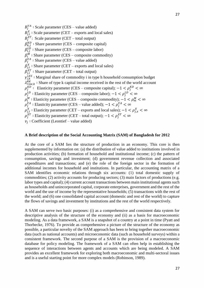
27

27

𝐵𝑗𝑉𝐴 ∶ Scale parameter (CES – value added)

𝐵𝑗,𝑖𝑋 ∶ Scale parameter (CET – exports and local sales)

𝐵𝑗𝑋𝑇: Scale parameter (CET – total output)

𝛽𝑘,𝑗𝐾𝐷 ∶ Share parameter (CES – composite capital)

𝛽𝑙,𝑗𝐿𝐷 ∶ Share parameter (CES – composite labor)

𝛽𝑖𝑀 ∶ Share parameter (CES – composite commodity)

𝛽𝑗𝑉𝐴 ∶ Share parameter (CES – value added)

𝛽𝑗,𝑖𝑋 ∶ Share parameter (CET – exports and local sales)

𝛽𝑗,𝑖𝑋𝑇 ∶ Share parameter (CET – total output)

𝛾𝑖,ℎ𝐿𝐸𝑆 ∶ Marginal share of commodity i in type h household consumption budget

𝜆𝑟𝑜𝑤,𝑘𝑅𝐾 ∶ Share of type k capital income received in the rest of the world account

𝜌𝑗𝐾𝐷 ∶ Elasticity parameter (CES – composite capital); −1 < 𝜌𝑗

𝐾𝐷 < ∞

𝜌𝑗𝐿𝐷 ∶ Elasticity parameter (CES – composite labor); −1 < 𝜌𝑗

𝐿𝐷 < ∞

𝜌𝑖𝑀 ∶ Elasticity parameter (CES – composite commodity); −1 < 𝜌𝑚

𝑀 < ∞

𝜌𝑗𝑉𝐴 ∶ Elasticity parameter (CES – value added); −1 < 𝜌𝑗

𝑉𝐴 < ∞

𝜌𝑗,𝑖𝑋 ∶ Elasticity parameter (CET – exports and local sales); −1 < 𝜌𝑗,𝑥

𝑋 < ∞

𝜌𝑗𝑋𝑇 ∶ Elasticity parameter (CET – total output); −1 < 𝜌𝑗

𝑋𝑇 < ∞

𝑣𝑗 ∶ Coefficient (Leontief – value added)

A Brief description of the Social Accounting Matrix (SAM) of Bangladesh for 2012

At the core of a SAM lies the structure of production in an economy. This core is then

supplemented by information on: (a) the distribution of value added to institutions involved in

production activities; (b) formation of household and institutional income; (c) the pattern of

consumption, savings and investment; (d) government revenue collection and associated

expenditures and transactions; and (e) the role of the foreign sector in the formation of

additional incomes for household and institutions. In particular, the accounting matrix of a

SAM identifies economic relations through six accounts: (1) total domestic supply of

commodities; (2) activity accounts for producing sectors; (3) main factors of productions (e.g.

labor types and capital); (4) current account transactions between main institutional agents such

as households and unincorporated capital, corporate enterprises, government and the rest of the

world and the use of income by the representative households; (5) transactions with the rest of

the world; and (6) one consolidated capital account (domestic and rest of the world) to capture

the flows of savings and investment by institutions and the rest of the world respectively.

A SAM can serve two basic purposes: (i) as a comprehensive and consistent data system for

descriptive analysis of the structure of the economy and (ii) as a basis for macroeconomic

modeling. As a data framework, a SAM is a snapshot of a country at a point in time (Pyatt and

Thorbecke, 1976). To provide as comprehensive a picture of the structure of the economy as

possible, a particular novelty of the SAM approach has been to bring together macroeconomic

data (such as national accounts) and microeconomic data (such as household surveys) within a

consistent framework. The second purpose of a SAM is the provision of a macroeconomic

database for policy modeling. The framework of a SAM can often help in establishing the

sequence of interactions between agents and accounts which are being modeled. A SAM

provides an excellent framework for exploring both macroeconomic and multi-sectoral issues

and is a useful starting point for more complex models (Robinson, 1989).

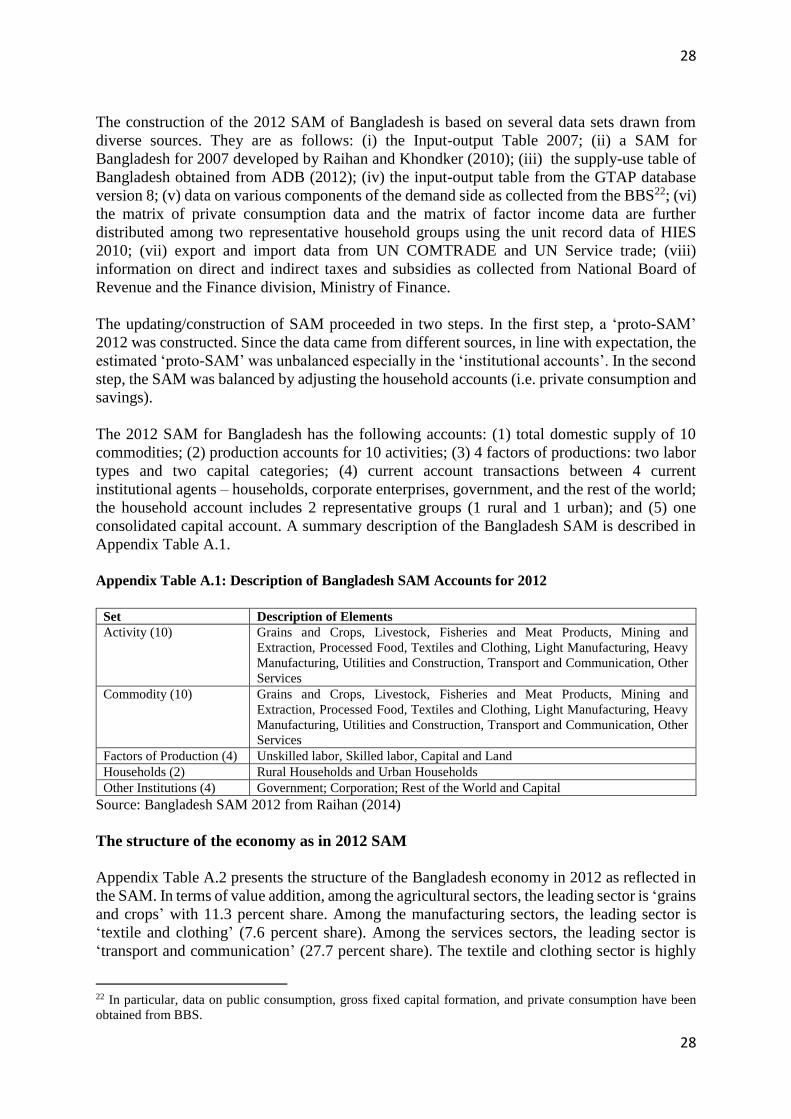
28

28

The construction of the 2012 SAM of Bangladesh is based on several data sets drawn from

diverse sources. They are as follows: (i) the Input-output Table 2007; (ii) a SAM for

Bangladesh for 2007 developed by Raihan and Khondker (2010); (iii) the supply-use table of

Bangladesh obtained from ADB (2012); (iv) the input-output table from the GTAP database

version 8; (v) data on various components of the demand side as collected from the BBS22; (vi)

the matrix of private consumption data and the matrix of factor income data are further

distributed among two representative household groups using the unit record data of HIES

2010; (vii) export and import data from UN COMTRADE and UN Service trade; (viii)

information on direct and indirect taxes and subsidies as collected from National Board of

Revenue and the Finance division, Ministry of Finance.

The updating/construction of SAM proceeded in two steps. In the first step, a ‘proto-SAM’

2012 was constructed. Since the data came from different sources, in line with expectation, the

estimated ‘proto-SAM’ was unbalanced especially in the ‘institutional accounts’. In the second

step, the SAM was balanced by adjusting the household accounts (i.e. private consumption and

savings).

The 2012 SAM for Bangladesh has the following accounts: (1) total domestic supply of 10

commodities; (2) production accounts for 10 activities; (3) 4 factors of productions: two labor

types and two capital categories; (4) current account transactions between 4 current

institutional agents – households, corporate enterprises, government, and the rest of the world;

the household account includes 2 representative groups (1 rural and 1 urban); and (5) one

consolidated capital account. A summary description of the Bangladesh SAM is described in

Appendix Table A.1.

Appendix Table A.1: Description of Bangladesh SAM Accounts for 2012

Set Description of Elements

Activity (10) Grains and Crops, Livestock, Fisheries and Meat Products, Mining and

Extraction, Processed Food, Textiles and Clothing, Light Manufacturing, Heavy

Manufacturing, Utilities and Construction, Transport and Communication, Other

Services

Commodity (10) Grains and Crops, Livestock, Fisheries and Meat Products, Mining and

Extraction, Processed Food, Textiles and Clothing, Light Manufacturing, Heavy

Manufacturing, Utilities and Construction, Transport and Communication, Other

Services

Factors of Production (4) Unskilled labor, Skilled labor, Capital and Land

Households (2) Rural Households and Urban Households

Other Institutions (4) Government; Corporation; Rest of the World and Capital

Source: Bangladesh SAM 2012 from Raihan (2014)

The structure of the economy as in 2012 SAM

Appendix Table A.2 presents the structure of the Bangladesh economy in 2012 as reflected in

the SAM. In terms of value addition, among the agricultural sectors, the leading sector is ‘grains

and crops’ with 11.3 percent share. Among the manufacturing sectors, the leading sector is

‘textile and clothing’ (7.6 percent share). Among the services sectors, the leading sector is

‘transport and communication’ (27.7 percent share). The textile and clothing sector is highly

22 In particular, data on public consumption, gross fixed capital formation, and private consumption have been

obtained from BBS.

29

29

export oriented. The export basket is highly concentrated as 88.1 percent of exports come from

‘textile and clothing’. The heavy manufacturing sector is highly import-dependent. As for tariff

rates, agricultural sectors have much lower tariff rates than the manufacturing sectors.

Appendix Table A.2: Structure of the Bangladesh economy as reflected in the SAM 2012

Sectors

1 2 3 4 5 6

Vi/TV Ei/Oi Ei/TE Mi/Oi Mi/TM TAR

Grains and Crops 11.33 0.42 0.56 9.09 8.05 4.52

Livestock, Fisheries and Meat Products 1.25 0.07 0.01 2.25 0.25 8.22

Mining and Extraction 6.60 0.16 0.08 2.20 0.75 7.61

Processed Food 1.34 1.53 1.59 15.96 10.87 13.38

Textiles and Clothing 7.55 51.68 88.12 17.57 19.70 25.33

Light Manufacturing 1.74 2.41 1.44 20.83 8.22 19.59

Heavy Manufacturing 0.99 1.17 1.26 60.96 43.16 11.77

Utilities and Construction 16.86 - - - - -

Transport and Communication 27.65 2.87 6.30 2.42 3.49 -

Other Services 24.69 0.28 0.63 3.65 5.52 -

Total 100.00 ― 100.00 ― 100.00 ―

Note: Vi=sectoral value added, TV=total value added, Ei=sectoral export, Oi=sectoral output, TE=total export,

Mi=sectoral import, TM=total import, TAR=tariff rate, All figures are expressed in percentages.

Source: Raihan (2014)