the manual jeffrey t. leek, eva monsen, alan r. dabney, and
TRANSCRIPT

THE MANUAL
Jeffrey T. Leek, Eva Monsen,
Alan R. Dabney, and John D. Storey
Department of Biostatistics
Department of Genome Sciences
University of Washington
http://faculty.washington.edu/jstorey/edge/
0
Contents
1 Overview 4
1.1 Contributors . . . . . . . . . . . . . . . . . . . . . . . . . . . . . . . . . . . . . . . . 4
1.2 Citations . . . . . . . . . . . . . . . . . . . . . . . . . . . . . . . . . . . . . . . . . . 5
2 Getting Started 5
2.1 Installing and Starting EDGE . . . . . . . . . . . . . . . . . . . . . . . . . . . . . . . 5
2.2 The Main EDGE Window . . . . . . . . . . . . . . . . . . . . . . . . . . . . . . . . . . 6
3 Formatting and Loading Data 7
3.1 Data File Format . . . . . . . . . . . . . . . . . . . . . . . . . . . . . . . . . . . . . . 7
3.2 Loading Data . . . . . . . . . . . . . . . . . . . . . . . . . . . . . . . . . . . . . . . . 8
3.3 Saving the EDGE Session as an R Image . . . . . . . . . . . . . . . . . . . . . . . . . . 9
3.4 Example Data Sets . . . . . . . . . . . . . . . . . . . . . . . . . . . . . . . . . . . . . 9
4 Data Preprocessing and Visualization 10
4.1 Imputing Missing Data . . . . . . . . . . . . . . . . . . . . . . . . . . . . . . . . . . . 10
4.2 Viewing Covariate Information . . . . . . . . . . . . . . . . . . . . . . . . . . . . . . 10
4.3 Transforming Data . . . . . . . . . . . . . . . . . . . . . . . . . . . . . . . . . . . . . 10
4.4 Display Boxplots . . . . . . . . . . . . . . . . . . . . . . . . . . . . . . . . . . . . . . 11
5 Pattern Discovery and Display 11
5.1 Hierarchical Clustering . . . . . . . . . . . . . . . . . . . . . . . . . . . . . . . . . . . 11
5.2 Eigengenes and Eigenarrays . . . . . . . . . . . . . . . . . . . . . . . . . . . . . . . . 12
6 Identifying Differentially Expressed Genes 13
6.1 Types of Differential Expression . . . . . . . . . . . . . . . . . . . . . . . . . . . . . . 13
6.2 Static Sampling Studies . . . . . . . . . . . . . . . . . . . . . . . . . . . . . . . . . . 14
6.3 Time Course Studies . . . . . . . . . . . . . . . . . . . . . . . . . . . . . . . . . . . . 14
6.4 Continuous Response Studies . . . . . . . . . . . . . . . . . . . . . . . . . . . . . . . 15
6.5 Matched Design Studies . . . . . . . . . . . . . . . . . . . . . . . . . . . . . . . . . . 16
6.6 Displaying, Analyzing and Saving Significant Genes . . . . . . . . . . . . . . . . . . . 16
7 Using the EDGE for Excel Add-In 17
7.1 Introduction . . . . . . . . . . . . . . . . . . . . . . . . . . . . . . . . . . . . . . . . . 17
7.2 Installing the Add-In . . . . . . . . . . . . . . . . . . . . . . . . . . . . . . . . . . . . 18
7.3 Using the Add-In . . . . . . . . . . . . . . . . . . . . . . . . . . . . . . . . . . . . . . 18
1

7.4 Removing the Add-In . . . . . . . . . . . . . . . . . . . . . . . . . . . . . . . . . . . 19
8 Frequently Asked Questions 19
9 Getting Further Help 20
2
List of Figures
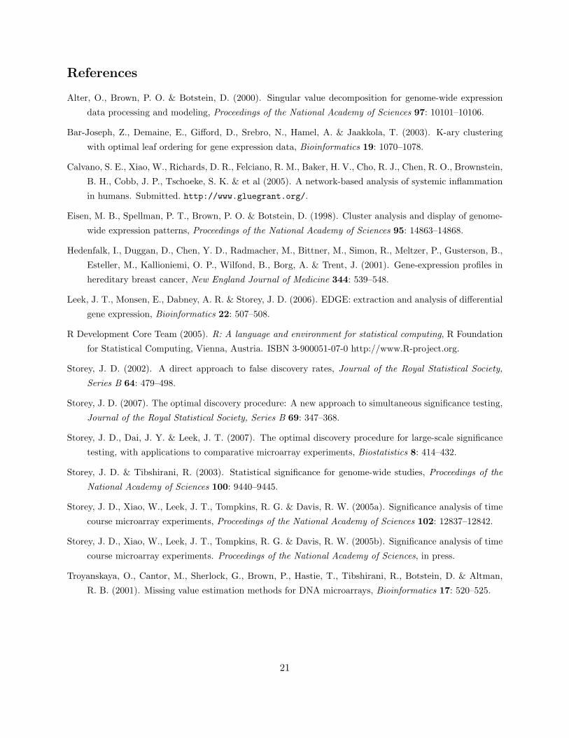
1 A comparison between EDGE and five leading procedures for identifying differentially
expression genes applied to the BRCA data set of Section 3.4. For each q-value (false
discovery rate) cut-off, the number of genes found to be significant is plotted for each
procedure. See Storey et al. (2007) for comparisons based on a 3-sample analysis,
where improvements are even greater. . . . . . . . . . . . . . . . . . . . . . . . . . . 22
2 Main EDGE window. The menu lists the eight possible analysis tasks to perform.
The main window remains present for all tasks except for clustering and displaying
differential expression results. . . . . . . . . . . . . . . . . . . . . . . . . . . . . . . 23
3 Loading data and saving the set as an R object. . . . . . . . . . . . . . . . . . . . . 24
4 Missing data imputation. . . . . . . . . . . . . . . . . . . . . . . . . . . . . . . . . . 25
5 Display covariate data. . . . . . . . . . . . . . . . . . . . . . . . . . . . . . . . . . . 26
6 Transform data. . . . . . . . . . . . . . . . . . . . . . . . . . . . . . . . . . . . . . . 27
7 Display boxplots of data grouped by any covariate or by the order of arrays in the
data file. . . . . . . . . . . . . . . . . . . . . . . . . . . . . . . . . . . . . . . . . . . 28
8 An example of the displayed boxplots. . . . . . . . . . . . . . . . . . . . . . . . . . 29
9 Perform hierarchical clustering on the entire data set or a subset of differentially
expressed genes. . . . . . . . . . . . . . . . . . . . . . . . . . . . . . . . . . . . . . . 30
10 An example of a displayed hierarchical clustering. . . . . . . . . . . . . . . . . . . . 31
11 Perform an “eigen-analysis” of the expression data set. . . . . . . . . . . . . . . . . 32
12 An example of a displayed eigen-genes. . . . . . . . . . . . . . . . . . . . . . . . . . 33
13 The main window for performing an EDGE differential expression analysis. . . . . . 34
14 Time course sampling settings. . . . . . . . . . . . . . . . . . . . . . . . . . . . . . . 35
15 Settings in the differential expression analysis when there is “matching” between
arrays. . . . . . . . . . . . . . . . . . . . . . . . . . . . . . . . . . . . . . . . . . . . 36
16 Display of differential expression results. It is possible to view significance measure
information (q-value plots and p-value histogram), access NCBI for any significant
gene, or cluster the differentially expressed genes. Significance cut-offs can be ad-
justed according to the user’s preference. . . . . . . . . . . . . . . . . . . . . . . . . 37
17 Example of an Excel spreadsheet that is ideally formatted for EDGE. Note the blank
row between the covariates and data. . . . . . . . . . . . . . . . . . . . . . . . . . . 38
3

1 Overview
EDGE is a point-and-click, open-source software package for the analysis of expression data. The
main purpose of the software is to perform significance analyses on comparative microarray experi-
ments. Because there are many steps that need to be performed along with a significance analysis,
we have attempted to include what we have found to be the core analysis procedures. In addition
to the significance analysis procedures for identifying differentially expressed genes, EDGE includes
functions for data visualization, transformation, exploratory analysis, and NCBI queries. All pro-
cedures implemented in the software are based on sound statistical procedures that have appeared
or are scheduled to appear in peer-reviewed articles. EDGE is cross-platform compatible (Windows,
Mac, Linux and Unix), running on top of the R statistical software package (R Development Core
Team 2005). It does not require the user to employ any closed-source software.
Using new statistical theory (Storey 2007, Storey et al. 2007), EDGE allows one to identify genes
that are differentially expressed between two or more different biological conditions (e.g., healthy
versus diseased tissue). There are already a number of software packages to perform this type of
analysis. However, EDGE is based on the Optimal Discovery Procedure (ODP) that we recently
introduced, which is significantly different from existing approaches. Whereas previously existing
methods employ statistics that are essentially designed for testing one gene at a time (e.g., t-
statistics and F-statistics), the ODP uses all relevant information from all genes in order to test
each one for differential expression. The improvements in power are substantial; Figure 1 shows a
comparison between EDGE and five leading software packages, based on a well-known breast cancer
expression study (Hedenfalk et al. 2001).
EDGE also allows one to perform significance analysis on time course experiments (Storey et al.
2005a). Two types of time course significance analyses are possible. One type allows the user to
test for genes whose expression changes over time. The other allows the user to identify genes
who show different expression over time between two or more biological conditions. Even though
some significance analysis packages allow for users to enter information about time points, we have a
rigorously developed set of methodology that was recently published in Storey et al. (2005b). There
are many things that can go wrong when applying methods originally developed for traditional
“static” analyses to time course experiments, so it is important to use a method that has been
specifically designed and justified for this setting.
1.1 Contributors
EDGE was written by Jeffrey Leek, Eva Monsen, Alan Dabney, and John Storey.
4
1.2 Citations
The “static sampling” differential expression analysis is carried out according to Storey et al. (2007).
The “time course” differential expression analysis is carried out according to Storey et al. (2005a).
Leek et al. (2006) can be used to cite this software in general. The other previously existing methods
that we have implemented into EDGE are cited and described below.
2 Getting Started
2.1 Installing and Starting EDGE
Windows Installation
1. Download the latest version of R from http://cran.r-project.org/.
2. Download the latest version of the EDGE installation executable for Windows from the down-
load web site provided when obtaining a license.
3. Double-click this installation file and follow all default settings. An EDGE icon will appear on
your desktop and in the start menu, and all EDGE files will be stored in
C:\Program Files\R\EDGE\.
4. Double-click the EDGE icon to start the software. An EDGE window will open as in Figure 2.
Its corresponding R window will also open but will be minimized.
Macintosh Installation
1. Install X11 from the installation dvd that comes with all Macs.
2. Install the latest version of R from http://cran.r-project.org/. We recommend that you
perform a default installation.
3. Download the most recent EDGE bundle from the download web site provided when obtaining
a license; if the edge X.Y.Z.tar.gz file doesn’t automatically unstuff, double click it and an
EDGE folder will appear.
4. Move the resulting EDGE folder to your Applications folder.
5. Inside the EDGE folder is a blue EDGE.app file. Drag this icon to your dock.
6. Click on the icon to start EDGE . We recommend that you close all X11 windows before
starting EDGE.
5
Linux/Unix Installation
1. Install the latest version of R from http://cran.r-project.org/. Also make certain that
the latest version of Tcl/Tk is installed on your operating system.
2. Download the most recent EDGE bundle from the download web site provided when obtaining
a license.
3. Open a terminal, cd to the directory where edge X.Y.Z.tar.gz is saved and type:
gzip -d edge X.Y.Z.tar.gz
tar xvf edge X.Y.Z.tar
4. To compile EDGE, type make install in the edge X.Y.Z/src/ directory.
5. To start EDGE, cd to the EDGE/ directory that was just created and type R. After the R session
starts, type source("edge.r") at the R prompt. To launch the graphical interface, then type
edge() at the R prompt.
2.2 The Main EDGE Window
Figure 2 shows the main EDGE window that will appear once the software is started. There are
eight different functions that can be performed:
• Load/Save Expression Data and Covariates
• Impute Missing Data
• View Covariates
• Transform Data
• Display Boxplots
• Display Hierarchical Clustering
• Display Eigengenes and Eigenarrays
• Identify Differentially Expressed Genes
The remaining sections explain how to employ each of these functions. In order to initiate a
function, select it with your mouse and press GO. The main window will remain visible for all
functions except for Display Hierarchical Clustering. Information and error messages will
appear in the message box of the main EDGE window.
6

3 Formatting and Loading Data
3.1 Data File Format
There is a special format for the expression data files loaded into EDGE. All data files should be
saved as tab-delimited text files, which can easily done from Microsoft Excel or R. There should be
two files for any analysis: a file containing the expression measurements and a file containing the
relevant variables (called “covariates”) that give information about each array.
The expression input file. The first file is the expression input file and should be formated
according to the examples below in Tables 1 and 2. The first row consists of descriptions of each
column. The array names will likely be specific to some nomenclature your lab has adopted. In the
simplest format (Table 1), the first column consists of gene names for the genes being analyzed. If
the user desires to use the web searching option after differential expression analysis, the gene names
should be either UIDs or accession numbers. The remaining columns are filled with the appropriate
expression values. The second format (Table 2) is similar to the first, except that a “Description”
column is included as the second column of the expression input. The description column may
consist of a small phrase describing each gene, or other important information. It is important to
emphasize that entries within a row must be tab-delimited for either type of file format.
Table 1: Example expression data input file.Gene Name Array1 Array2 Array3 Array4 Array5 Array6
300001 at 3033.46 726.092 1718.15 999.01 1132.34 1128.04
300002 s at 1087.45 789.734 1106.86 956.63 1253.77 1298.48
300003 at 12238.7 4868.51 8166.45 8277.71 7760.86 10289.5
300004 s at 1111.43 936.013 928.879 1570.06 1630.54 1941.9...
......
......
......
308136 s at 1840.85 626.16 817.791 1361.28 1216.51 1511.81
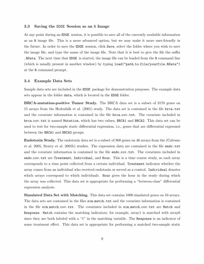
The covariate input file. The second file is the covariate input file and should be formatted as
in Table 3. Again, this file should be saved as a tab-delimited text file. The first row should be
identical to the first row of the expression data file. The top left entry is not actually used, so we
have written it as “Cov Name” here instead of “Gene Name”; one can also leave this particular
entry blank. Each subsequent row should contain the name for a covariate, followed by its values
across the arrays. If the covariate is categorical (meaning that it describes unordered classes), then
one can code this variable by different numbers or by different words. For example, rows 2, 3, and
7
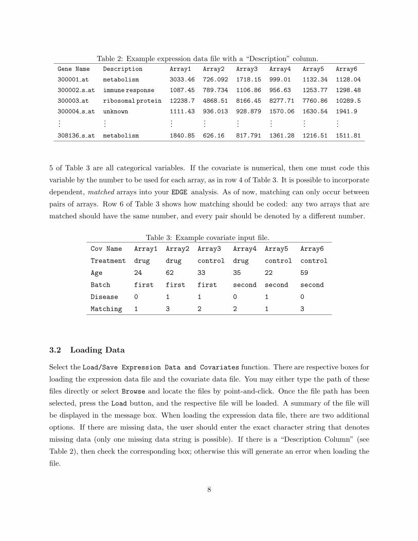
Table 2: Example expression data file with a “Description” column.Gene Name Description Array1 Array2 Array3 Array4 Array5 Array6
300001 at metabolism 3033.46 726.092 1718.15 999.01 1132.34 1128.04
300002 s at immune response 1087.45 789.734 1106.86 956.63 1253.77 1298.48
300003 at ribosomal protein 12238.7 4868.51 8166.45 8277.71 7760.86 10289.5
300004 s at unknown 1111.43 936.013 928.879 1570.06 1630.54 1941.9...
......
......
......
...
308136 s at metabolism 1840.85 626.16 817.791 1361.28 1216.51 1511.81
5 of Table 3 are all categorical variables. If the covariate is numerical, then one must code this
variable by the number to be used for each array, as in row 4 of Table 3. It is possible to incorporate
dependent, matched arrays into your EDGE analysis. As of now, matching can only occur between
pairs of arrays. Row 6 of Table 3 shows how matching should be coded: any two arrays that are
matched should have the same number, and every pair should be denoted by a different number.
Table 3: Example covariate input file.Cov Name Array1 Array2 Array3 Array4 Array5 Array6
Treatment drug drug control drug control control
Age 24 62 33 35 22 59
Batch first first first second second second
Disease 0 1 1 0 1 0
Matching 1 3 2 2 1 3
3.2 Loading Data
Select the Load/Save Expression Data and Covariates function. There are respective boxes for
loading the expression data file and the covariate data file. You may either type the path of these
files directly or select Browse and locate the files by point-and-click. Once the file path has been
selected, press the Load button, and the respective file will be loaded. A summary of the file will
be displayed in the message box. When loading the expression data file, there are two additional
options. If there are missing data, the user should enter the exact character string that denotes
missing data (only one missing data string is possible). If there is a “Description Column” (see
Table 2), then check the corresponding box; otherwise this will generate an error when loading the
file.
8
3.3 Saving the EDGE Session as an R Image
At any point during an EDGE session, it is possible to save all of the currently available information
as an R image file. This is a more advanced option, but we may make it more user-friendly in
the future. In order to save the EDGE session, click Save, select the folder where you wish to save
the image file, and type the name of the image file. Note that it is best to give the file the suffix
.RData. The next time that EDGE is started, the image file can be loaded from the R command line
(which is usually present in another window) by typing load("path to file/yourfile.RData")
at the R command prompt.
3.4 Example Data Sets
Sample data sets are included in the EDGE package for demonstration purposes. The example data
sets appear in the folder data, which is located in the EDGE folder.
BRCA-mutation-positive Tumor Study. The BRCA data set is a subset of 3170 genes on
15 arrays from the Hedenfalk et al. (2001) study. The data set is contained in the file brca.txt
and the covariate information is contained in the file brca cov.txt. The covariate included in
brca cov.txt is named Mutation, which has two values, BRCA1 and BRCA2. This data set can be
used to test for two-sample static differential expression, i.e., genes that are differential expressed
between the BRCA1 and BRCA2 groups.
Endotoxin Study. The endotoxin data set is a subset of 800 genes on 46 arrays from the (Calvano
et al. 2005, Storey et al. 2005b) studies. The expression data are contained in the file endo.txt
and the covariate information is contained in the file endo cov.txt. The covariates included in
endo cov.txt are Treatment, Individual, and Hour. This is a time course study, so each array
corresponds to a time point collected from a certain individual. Treatment indicates whether the
array comes from an individual who received endotoxin or served as a control. Individual denotes
which arrays correspond to which individuals. Hour gives the hour in the study during which
the array was collected. This data set is appropriate for performing a “between-class” differential
expression analysis.
Simulated Data Set with Matching. This data set contains 1000 simulated genes on 10 arrays.
The data sets are contained in the files sim match.txt and the covariate information is contained
in the file sim match cov.txt. The covariates included in sim match cov.txt are Match and
Response. Match contains the matching indicators; for example, array1 is matched with array6
since they are both labeled with a “1” in the matching variable. The Response is an indicator of
some treatment effect. This data set is appropriate for performing a matched two-sample static
9
differential expression analysis. This data set has missing values denoted by NA, so it can be used
to test the missing data imputation function.
4 Data Preprocessing and Visualization
4.1 Imputing Missing Data
Many methods for analyzing gene expression microarray experiments are not designed to handle
missing data directly. “K nearest neighbor” (KNN) imputation replaces the missing expression
values for a gene using expression information from the K “most similar” complete genes, where
a complete gene has no missing expression values in the data set. The K most similar complete
genes are the K complete genes that are closest in Euclidean distance to the gene with missing
values (Troyanskaya et al. 2001). The missing expression measurement on an array is imputed as
the mean of the measurements from the K nearest complete genes for that array. To open the
imputation window, select Impute Missing Data in the main menu, and press GO. You should now
see a window similar to Figure 4.
Click CALCULATE MISSING DATA STATISTICS to calculate and display the percent of missing
values in genes, arrays, and overall. Two settings are available in the KNN parameters frame. Set
the percent of missing values to tolerate in a gene to eliminate genes in the data set with a percent
of missing values higher than the tolerance. If no genes should be eliminated from the data set,
the tolerance should be set to 100. Set the number of nearest neighbors to use to determine the
number of nearest neighbors used for imputing missing values, up to the number of complete genes
in the data set. After setting the KNN parameters click GO to perform the imputation. Click DONE
to return to the main menu.
4.2 Viewing Covariate Information
After loading expression data and covariate information, check the covariate information for accu-
racy by selecting View Covariates from the main menu and pressing GO. You should see a window
similar to Figure 5. The covariate names are displayed, followed by the values currently loaded into
EDGE. Click DONE to return to the main menu after ensuring the covariate information is correct.
4.3 Transforming Data
It is sometimes desirable to center and/or scale the expression measurements from each array. To
open the data transformation window, select Transform Data from the main menu and click GO.
You should see a window similar to Figure 6.
10
There are three standard transformations that can be performed by the EDGE software. Choose
the appropriate options for taking the log2 transform, mean or median centering, and standard
deviation or absolute deviation scaling. One may want to add a small positive constant to all
of the expression measurements before taking the log2 transform. This can help to avoid taking
the log2 of zero or a negative number (which is undefined) and it can also help to stabilize the
variance of genes with low expression values. After setting the options, click GO to perform the data
transformation. Click DONE to return to the main menu.
4.4 Display Boxplots
Boxplots are a useful for viewing the distribution of large numbers of expression measurements.
Boxplots indicate the median expression and give an indication of the spread of expression mea-
surements within a defined group (e.g., an array). To view boxplots, select Display Boxplots
from the main menu and click GO. You should see a window like Figure 7. It is possible to group
the expression measurements by any covariate or by the arrays themselves. Choose a variable from
the Boxplots by Covariate frame to display one boxplot for each level of that covariate, or select
Data Array Order to display one boxplot per array. Choose the number of boxplots to display per
screen, up to the maximum displayed in parentheses.
Click OK to display the number of boxplots you set above. You should see a plot similar to
Figure 8; above each boxplot appears the value of the covariate (or the array number). To see the
next set of boxplots, click NEXT BOXPLOT and continue until boxplots for all values of the covariate
(or all arrays) have been displayed. Click DONE to return to the main menu.
5 Pattern Discovery and Display
5.1 Hierarchical Clustering
Hierarchical clustering organizes genes into groups with similar gene expression patterns (Eisen
et al. 1998). Initially, each gene represents its own group. Clusters are then built one gene at
a time, where each gene is added to the group to which it is most similar, or “nearest.” When
a group already includes more than one gene, EDGE uses “centroid linkage” to compute distances
to that group. To open the clustering window, select Display Hierarchical Clustering in the
main menu, then press GO. You should now see a window similar to Figure 9.
Two optional settings are available in the Cluster Options frame. EDGE uses one of two
distance metrics. The squared Euclidean distance between two genes is the sum of squared differ-
ences between each component, while the Correlation distance between two genes is one minus
11

their sample correlation. After clustering, EDGE reorders the genes, so that adjacent elements in
a graphical display are most similar. Because the Optimal ordering (Bar-Joseph et al. 2003) is
very computationally intensive, a Heuristic ordering routine (Eisen et al. 1998) is available as an
alternative. Once you have specified the options, click CLUSTER to begin. Progress will be moni-
tored in the Clustering progress frame. Click CANCEL at any time if you would like to stop the
computation.
Once completed, you can view the results in a heatmap. Several options are available in frame
Plot Options. Choose whether you would like gene and/or array Labels included on the plot.
Note that the plot will quickly become overly crowded if too many labels are included. The choice
of Coloring can have a large impact on the visual interpretation of your results. If there are a few
expression measurements that are extreme relative to the others, then the majority of observations
will be assigned the same (or very similar) color. Choosing Logarithmic color scale should help
in this situation. Similarly, you can choose between coloring by Value or Rank. Choosing Rank will
also help in the above situation. Under Scaling, Centering, and Transforms, you can Center
each gene around its mean, forcing all genes to be centered at zero. You can also remove extreme
values from the plot under Truncate data values. This can be done by specifying either an
Absolute cutoff or Multiples of standard deviation. For example, if you specify a cutoff of
2, then only expression measurements with values less than 2 will be included in the plot. Similarly,
if you specify a standard deviation of 3, then only measurements which fall within three standard
deviations of the overall mean will be plotted.
Once you have specified the plotting options, click PLOT. This will cause R to produce a plot
similar to Figure 10. Rows represent genes, and columns represent arrays. The dendogram on the
left describes the progression of the clustering routine, where branch lengths reflect the degree of
similarity between the connected objects. Colors range from blue on the low end of expression
measurements to red on the high end. In the cluster analysis of Figure 10, two large clusters are
apparent. In the larger cluster, there tends to be high expression in samples 1-7 and low expression
in samples 8-15. This relationship is switched in the smaller cluster. You can now SAVE PLOT AS
PDF or change some of the options and PLOT AGAIN. Click DONE to return to the main menu.
5.2 Eigengenes and Eigenarrays
Eigengenes are representations of common expression patterns across arrays (Alter et al. 2000).
Similarly, eigenarrays are representations of common expression profiles across genes. In mathe-
matical terms, an eigengene is composed of coefficients for a linear combination of the arrays which
accounts for a substantial amount of the total variation in the data. Similarly, an eigenarray is a
set of coefficients for a linear combination of the genes. Each eigengene is orthogonal to any other
12
eigengene, with the same relation holding for eigenarrays. The amount of variation accounted for
by each eigengene and eigenarray can be calculated. With m genes and n arrays, there will be n
eigengenes and n eigenarrays. To open the “eigen-analysis” window, select Display Eigengenes
and Eigenarrays in the main menu, then press GO. You should now see a window similar to Figure
11.
Select either Eigengenes or Eigenarrays under Plot. If you are interested in common expres-
sion patterns across something other than arrays, you can specify this under Plot by Variable.
For example, in Figure 11, the variables Treatment, Individual, and Hour are listed in addition to
Data Array Order. If Treatment is selected, for example, then eigengenes will describe common
expression patterns across treatment groups. You can specify the number of plots to display at a
time in Number to Plot.
Once you have specified all options, click OK. This will cause R to produce a plot similar to
Figure 12. In this case, eigengenes have been computed across arrays. The eigengene values are on
the y-axis, and array number is on the x-axis. The plot titles tell you the proportion of variation
accounted for by each eigengene. In this example, the first eigengene accounts for 61% of all
variation in the data. We can interpret this as meaning that the single most influential expression
pattern in these data roughly involves a change in the sign of expression between the first 25 arrays
and the last 20 arrays. Note that the direction of eigengene or eigenarray trends is irrelevant. In
particular, the first eigengene in Figure 12 could equivalently be represented by rotating all points
about the horizontal zero line. Click Next to display the next set of eigengenes or eigenarrays.
Click DONE to return to the main menu.
6 Identifying Differentially Expressed Genes
To perform a differential expression analysis, select the Identify Differentially Expressed
Genes option, then click GO. The differential expression window will appear as in Figure 8.
6.1 Types of Differential Expression
There are three experimental designs where EDGE can identify differentially expressed genes. The
first is a “static sampling” experiment, which means that the arrays have been collected from dis-
tinct biological groups and without respect to time. This has been the most common experimental
design up till this point. The goal is to identify genes that have a statistically significant difference
in average expression across these distinct biological groups. When a two-channel microarray sys-
tem is used, it is possible to measure gene expression from two populations of interest on a single
array. In this case, the arrays all come from a single “group” and a gene is said to be differentially
13

expressed if its average relative expression (as a log-scale ratio) is different than zero.
The second type of experiment is a time course experiment, where the arrays have been sampled
with respect to time from one or more distinct biological groups. If only one biological group has
been sampled, then the goal is to identify genes that show “within-class temporal differential
expression”, i.e., genes that show statistically significant changes in expression over time. If two or
more biological groups have been sampled, then the goal is to identify genes that show “between-
class temporal differential expression”, i.e., genes that show statistically significant differences in
expression over time between the various groups.
The third type of experiment is a “continuous response” design, which means that the arrays
have been collected from a continuously defined biological state and without respect to time. The
goal here is to identify genes whose expression shows a statistically significant change with respect to
this continuous response. For example, arrays may be sampled from individuals where their blood
pressure has been recorded, and the goal would be to identify genes whose expression changes with
blood pressure.
6.2 Static Sampling Studies
Figure 13 shows the window that opens when the user selects the differential expression function.
The top panel, Choose Class Variable, should be used to select the variable that identifies the
biological groups to be compared. If only one biological group has been sampled select None. Under
the next panel, Differential Expression Type, select Static (standard, non-time course
sampling).
The user may now click the button STATIC SAMPLING SETTINGS, but there are currently no
additional settings to apply. In the near future, there will be options to perform tests for over- or
under-expression alone. In addition, the user will be able to test for fold change above a certain
threshold by clicking the check box and entering the fold change of interest.
The significance calculation is based on randomly permuting the group labels, so under the
Number of null iterations panel the user should choose the number of null iterations to be
performed. If the total number of unique permutations is less than or equal to what the user has
chosen, then EDGE performs all unique permutations. It may be important to be able to reproduce
results exactly, in which case the user should choose a random seed under the Choose a seed for
reproducible results panel. Once these steps are performed, click GO and the calculations will
begin.
Information about the time remaining and percentage of calculations completed will be displayed
throughout the calculations. If the calculation needs to be canceled, then click CANCEL. If you
decide not to perform a differential expression analysis, then click DONE. Once the calculations are
14
completed, a results window will appear, which is described below in Section 6.6.
6.3 Time Course Studies
Figure 13 shows the window that opens when the user selects the differential expression function.
The top panel, Choose Class Variable, should be used to select the variable that identifies the
biological groups to be compared. If only one biological group has been sampled select None. Under
the next panel, Differential Expression Type, select Time Course.
The user may now click the button TIME COURSE SETTINGS, and the window will appear as
in Figure 14. You must select a covariate that denotes the time point at which each array was
sampled. This variable should be selected in the top panel, Choose covariate giving time
points. If individuals were sampled at more than one time point (making these arrays dependent),
then the variable denoting which individual corresponds to which array should be selected under
the second panel, Choose covariate corresponding to individuals.
At the bottom of the window, there are options regarding the type of spline that is used to
model the expression over time. The first option is to choose between a natural cubic spline or
polynomial spline. The natural cubic spline is suggested unless there are specific considerations
that merit use of the polynomial spline. If desired, the user can also choose the basis dimension for
the spline at the second option; if not specified the basis dimension will be chosen automatically.
In some cases, it may also be necessary to determine baseline differences in expression over time
in addition to changes over time. If this is the case, then click the button at the third option to
include the intercept in the analysis. It should be noted that also detecting baseline differences is
considerably more computationally intensive when longitudinal sampling has been employed, and
it should only be used where appropriate.
After choosing the appropriate options, click APPLY to return to the differential expression menu.
Click CANCEL to return to the differential expression menu without setting time course options.
Once these steps are performed, click GO and the calculations will begin. Information about
the time remaining and percentage of calculations completed will be displayed throughout the
calculations. If the calculation needs to be canceled, then click CANCEL. If you decide not to
perform a differential expression analysis, then click DONE. Once the calculations are completed, a
results window will appear, which is described below in Section 6.6.
6.4 Continuous Response Studies
Figure 13 shows the window that opens when the user selects the differential expression function.
The top panel, Choose Class Variable, should be set at None. A continuous response study
15
can be analyzed using a special set of choices for the time course options. Therefore, for the
Differential Expression Type panel, select Time Course.
Now click the button TIME COURSE SETTINGS, and the window will appear as in Figure 14.
The covariate that denotes the continuous response should be selected in the top panel, Choose
covariate giving time points. Under the second panel, Choose covariate corresponding
to individuals, select None.
At the bottom of the window, there are options regarding the type of spline that is used to
model the relationship of expression to the continuous response. The first option is to choose
between a natural cubic spline or polynomial spline. The natural cubic spline is suggested unless
there are specific considerations that merit use of the polynomial spline, such as a desire for easier
model interpretability. If desired, the user can also choose the basis dimension for the spline at the
second option; if not specified the basis dimension will be chosen automatically. The dimension is
defined so that a dimension of one is equivalent to a straight line, two equivalent to the complexity
of a quadratic, etc. It is almost always not going to be appropriate to include the intercept in the
analysis, so this box should not be checked.
After choosing the appropriate options, click APPLY to return to the differential expression menu.
Click CANCEL to return to the differential expression menu without setting any options.
Once these steps are performed, click GO and the calculations will begin. Information about
the time remaining and percentage of calculations completed will be displayed throughout the
calculations. If the calculation needs to be canceled, then click CANCEL. If you decide not to
perform a differential expression analysis, then click DONE. Once the calculations are completed, a
results window will appear, which is described below in Section 6.6.
6.5 Matched Design Studies
EDGE also permits the analysis of matched data for any of the above types of studies. After
completing the settings for your respective sampling type (but before clicking GO to start the
calculations), the user should click on MATCHED DESIGN SETTINGS. After the window shown in
Figure 15 appears, choose the matching variable and click APPLY. Click CANCEL to return to the
differential expression menu without setting matched design options. As of now, matching is only
possible when there are two biological groups (one member of each match per group). In the time
course setting, the individuals must have been sampled at the exact same time points. It is possible
to perform a continuous response analysis with matching because this analysis is a special case of
the time course “within-class” differential expression significance analysis method.
16
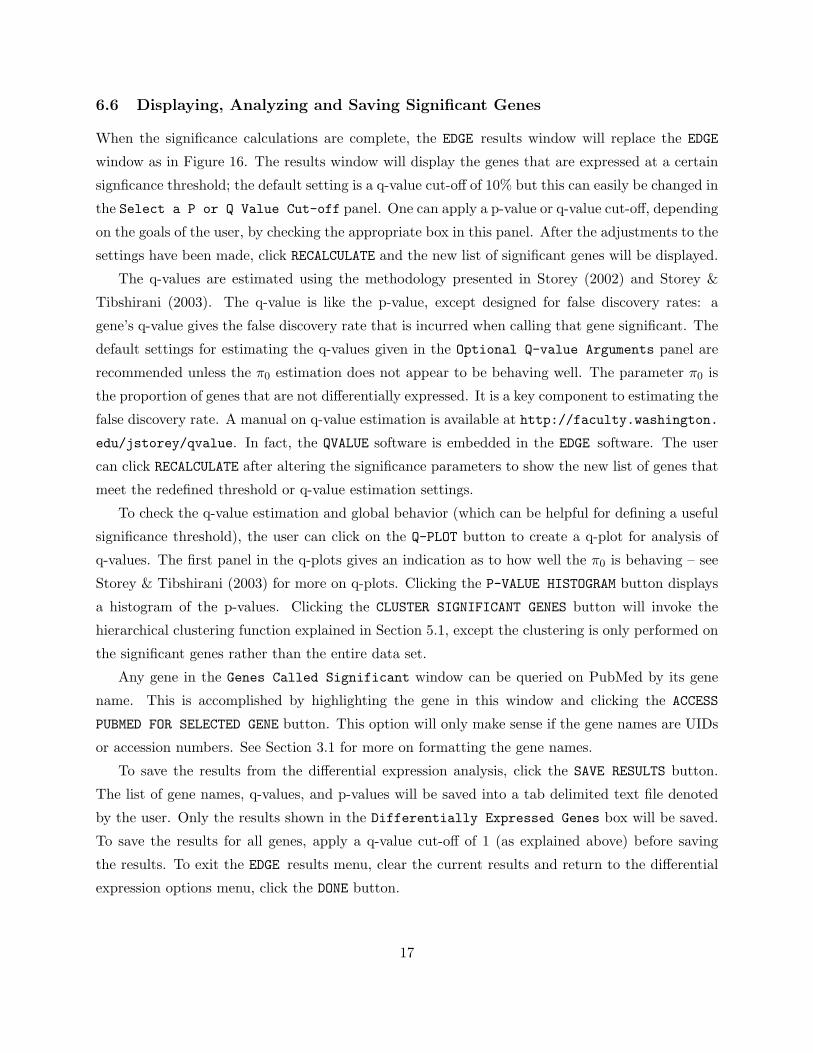
6.6 Displaying, Analyzing and Saving Significant Genes
When the significance calculations are complete, the EDGE results window will replace the EDGE
window as in Figure 16. The results window will display the genes that are expressed at a certain
signficance threshold; the default setting is a q-value cut-off of 10% but this can easily be changed in
the Select a P or Q Value Cut-off panel. One can apply a p-value or q-value cut-off, depending
on the goals of the user, by checking the appropriate box in this panel. After the adjustments to the
settings have been made, click RECALCULATE and the new list of significant genes will be displayed.
The q-values are estimated using the methodology presented in Storey (2002) and Storey &
Tibshirani (2003). The q-value is like the p-value, except designed for false discovery rates: a
gene’s q-value gives the false discovery rate that is incurred when calling that gene significant. The
default settings for estimating the q-values given in the Optional Q-value Arguments panel are
recommended unless the π0 estimation does not appear to be behaving well. The parameter π0 is
the proportion of genes that are not differentially expressed. It is a key component to estimating the
false discovery rate. A manual on q-value estimation is available at http://faculty.washington.
edu/jstorey/qvalue. In fact, the QVALUE software is embedded in the EDGE software. The user
can click RECALCULATE after altering the significance parameters to show the new list of genes that
meet the redefined threshold or q-value estimation settings.
To check the q-value estimation and global behavior (which can be helpful for defining a useful
significance threshold), the user can click on the Q-PLOT button to create a q-plot for analysis of
q-values. The first panel in the q-plots gives an indication as to how well the π0 is behaving – see
Storey & Tibshirani (2003) for more on q-plots. Clicking the P-VALUE HISTOGRAM button displays
a histogram of the p-values. Clicking the CLUSTER SIGNIFICANT GENES button will invoke the
hierarchical clustering function explained in Section 5.1, except the clustering is only performed on
the significant genes rather than the entire data set.
Any gene in the Genes Called Significant window can be queried on PubMed by its gene
name. This is accomplished by highlighting the gene in this window and clicking the ACCESS
PUBMED FOR SELECTED GENE button. This option will only make sense if the gene names are UIDs
or accession numbers. See Section 3.1 for more on formatting the gene names.
To save the results from the differential expression analysis, click the SAVE RESULTS button.
The list of gene names, q-values, and p-values will be saved into a tab delimited text file denoted
by the user. Only the results shown in the Differentially Expressed Genes box will be saved.
To save the results for all genes, apply a q-value cut-off of 1 (as explained above) before saving
the results. To exit the EDGE results menu, clear the current results and return to the differential
expression options menu, click the DONE button.
17

7 Using the EDGE for Excel Add-In
7.1 Introduction
Microsoft Excel is commonly used for organizing and preprocessing gene expression data. EDGE
can be invoked directly from an Excel worksheet, versions 2003 and later, on Windows or Macintosh
machines, with the click of a button. This chapter contains instructions for installing and using
the Add-In.
7.2 Installing the Add-In
The Add-In must be installed by hand from within Excel after the main EDGE application has
been installed. To install the Add-In,
1. Open Excel.
2. From the Tools menu, select Add-Ins.
3. Click Browse... (Windows) or Select... (Macintosh)
4. Find the EDGE program directory. On Windows, this is likely C:\Program Files\R\EDGE.On Macintosh, this should be /Applications/EDGE.
5. In the excel subdirectory, select EdgeModule.xla and click OK.
6. Make sure the checkbox next to EDGE for Excel Add-In is checked.
7. Click OK.
8. After you click OK, the add-in will install a menu entitled “EDGE” and a toolbar button.
7.3 Using the Add-In
1. Open your gene expression data spreadsheet.
2. The Add-In can handle data in most formats as long as all data is contained in the same
workbook. However, the Add-In most easily detects covariates and data if they are arranged as
follows: Covariates should be listed at the top of a worksheet, followed by a blank row, followed
by the expression data. Figure 17 provides an example, and so does the sample spreadsheet
brca example.xls. Of the visible arrays in the figure, 1, 2, and 3 are from individuals with the
BRCA1 mutation and 8 and 9 are from individuals with the BRCA2 mutation.
3. Select the area containing the covariates, gene names, and data.
18

4. From the EDGE menu, select Analyze with EDGE. Alternately, select the toolbar button
with the same caption.
5. You will see a dialog specifying the range containing covariates, and the cell range containing
data. Take a moment to verify the selections. To change the selections, click the button to
the right of the range text area.
6. Click Continue. The screen may flicker as the add-in saves temporary files for the covariates
and data. EDGE will start and your data will be automatically loaded. Follow the instructions
in the rest of this manual to complete your analysis.
7.4 Removing the Add-In
To remove the EDGE for Excel Add-In,
1. Open Excel.
2. From the Tools menu, select Add-Ins.
3. Uncheck the box next to EDGE for Excel Add-In.
4. Click OK.
The toolbar button and menu will be removed.
8 Frequently Asked Questions
1. What are the operating system requirements for EDGE?
EDGE is available for Windows, Macintosh OS X, Linux and Unix.
2. EDGE won’t start up on Mac OS X. I get an error including the line “Error in edge() :
TCLTK support is absent.”
Check to make sure that you have downloaded and installed X11.
3. Where can I go for help if I cannot get EDGE to work?
First, please visit the EDGE google group at http://groups-beta.google.com/group/edge-software
and read the old posts to try to find the answer to your problem. If you still are having dif-
ficulty, please post to the group, and include the error message, the operating system and
version of R you are using.
19

4. How do I view the p/q-values for all genes?
In the Differential Expression Results menu, choose a p/q-value cutoff of 1 to view all
p/q-values.
5. EDGE only prints the first 10 characters of the gene names on the Differential Expression
Results menu. How can I view the full gene names?
Only the first 10 characters are printed to the differential expression results screen for display
purposes. Save the differential expression results to view the full gene names.
6. How do I cite the EDGE software?
See the citations subsection of this document.
7. Will EDGE work on my laptop that was purchased in 1996?
Microarray analyses tend to be computationally intensive, so we recommend using a powerful
desktop computer for the most enjoyable EDGE experience.
9 Getting Further Help
A Google discussion group has been formed to handle help inquiries and suggestions. This is the
official mechanism for obtaining support. If you have a question, please first browse the previous
messages to see whether your question has already been addressed. Membership to the discussion
group is free with an email address. To join, go to
http://groups.google.com/group/edge-software
and click on Join this group. During the setup process, you can specify whether you want to be
notified by email when new messages are posted. Note that you can read past messages without
being a member. Membership is only required for posting.
20
References
Alter, O., Brown, P. O. & Botstein, D. (2000). Singular value decomposition for genome-wide expression
data processing and modeling, Proceedings of the National Academy of Sciences 97: 10101–10106.
Bar-Joseph, Z., Demaine, E., Gifford, D., Srebro, N., Hamel, A. & Jaakkola, T. (2003). K-ary clustering
with optimal leaf ordering for gene expression data, Bioinformatics 19: 1070–1078.
Calvano, S. E., Xiao, W., Richards, D. R., Felciano, R. M., Baker, H. V., Cho, R. J., Chen, R. O., Brownstein,
B. H., Cobb, J. P., Tschoeke, S. K. & et al (2005). A network-based analysis of systemic inflammation
in humans. Submitted. http://www.gluegrant.org/.
Eisen, M. B., Spellman, P. T., Brown, P. O. & Botstein, D. (1998). Cluster analysis and display of genome-
wide expression patterns, Proceedings of the National Academy of Sciences 95: 14863–14868.
Hedenfalk, I., Duggan, D., Chen, Y. D., Radmacher, M., Bittner, M., Simon, R., Meltzer, P., Gusterson, B.,
Esteller, M., Kallioniemi, O. P., Wilfond, B., Borg, A. & Trent, J. (2001). Gene-expression profiles in
hereditary breast cancer, New England Journal of Medicine 344: 539–548.
Leek, J. T., Monsen, E., Dabney, A. R. & Storey, J. D. (2006). EDGE: extraction and analysis of differential
gene expression, Bioinformatics 22: 507–508.
R Development Core Team (2005). R: A language and environment for statistical computing, R Foundation
for Statistical Computing, Vienna, Austria. ISBN 3-900051-07-0 http://www.R-project.org.
Storey, J. D. (2002). A direct approach to false discovery rates, Journal of the Royal Statistical Society,
Series B 64: 479–498.
Storey, J. D. (2007). The optimal discovery procedure: A new approach to simultaneous significance testing,
Journal of the Royal Statistical Society, Series B 69: 347–368.
Storey, J. D., Dai, J. Y. & Leek, J. T. (2007). The optimal discovery procedure for large-scale significance
testing, with applications to comparative microarray experiments, Biostatistics 8: 414–432.
Storey, J. D. & Tibshirani, R. (2003). Statistical significance for genome-wide studies, Proceedings of the
National Academy of Sciences 100: 9440–9445.
Storey, J. D., Xiao, W., Leek, J. T., Tompkins, R. G. & Davis, R. W. (2005a). Significance analysis of time
course microarray experiments, Proceedings of the National Academy of Sciences 102: 12837–12842.
Storey, J. D., Xiao, W., Leek, J. T., Tompkins, R. G. & Davis, R. W. (2005b). Significance analysis of time
course microarray experiments. Proceedings of the National Academy of Sciences, in press.
Troyanskaya, O., Cantor, M., Sherlock, G., Brown, P., Hastie, T., Tibshirani, R., Botstein, D. & Altman,
R. B. (2001). Missing value estimation methods for DNA microarrays, Bioinformatics 17: 520–525.
21
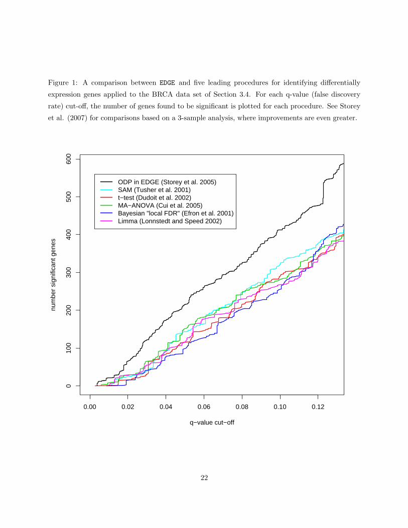
Figure 1: A comparison between EDGE and five leading procedures for identifying differentially
expression genes applied to the BRCA data set of Section 3.4. For each q-value (false discovery
rate) cut-off, the number of genes found to be significant is plotted for each procedure. See Storey
et al. (2007) for comparisons based on a 3-sample analysis, where improvements are even greater.
0.00 0.02 0.04 0.06 0.08 0.10 0.12
010
020
030
040
050
060
0
q−value cut−off
num
ber
sign
ifica
nt g
enes
ODP in EDGE (Storey et al. 2005)SAM (Tusher et al. 2001) t−test (Dudoit et al. 2002)MA−ANOVA (Cui et al. 2005)Bayesian "local FDR" (Efron et al. 2001)Limma (Lonnstedt and Speed 2002)
22

Figure 2: Main EDGE window. The menu lists the eight possible analysis tasks to perform. The
main window remains present for all tasks except for clustering and displaying differential expression
results.
23
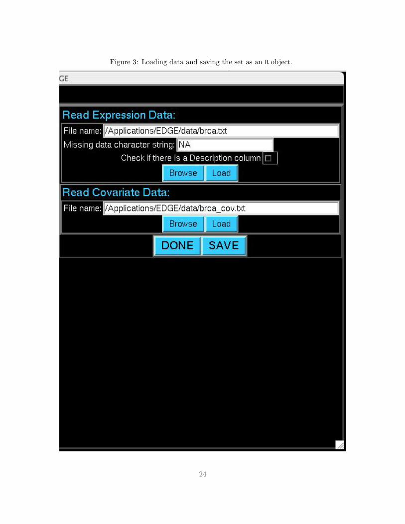
Figure 3: Loading data and saving the set as an R object.
24
Figure 4: Missing data imputation.
25
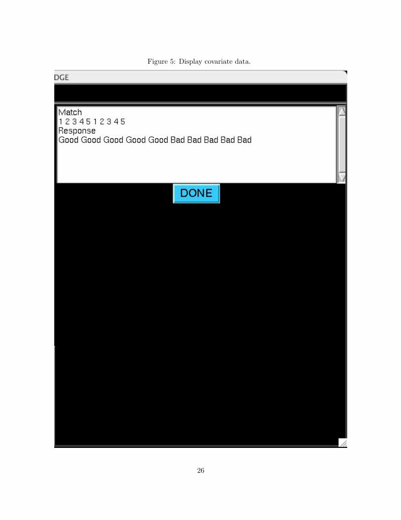
Figure 5: Display covariate data.
26
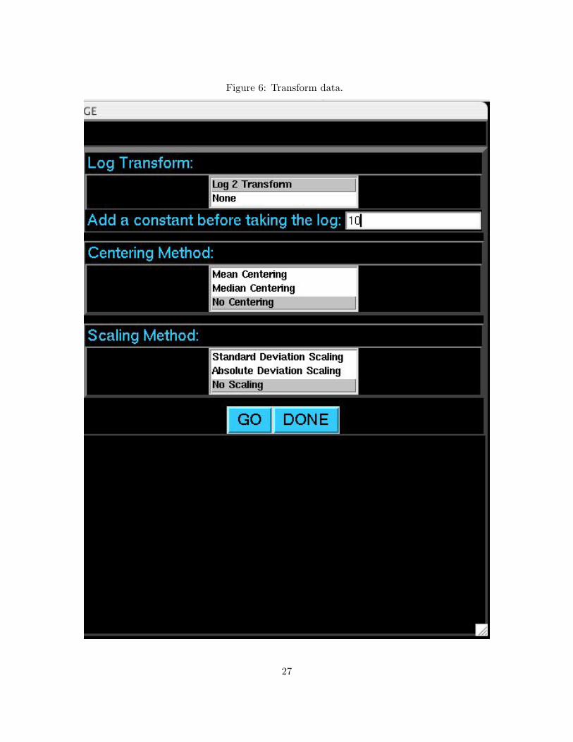
Figure 6: Transform data.
27

Figure 7: Display boxplots of data grouped by any covariate or by the order of arrays in the data
file.
28
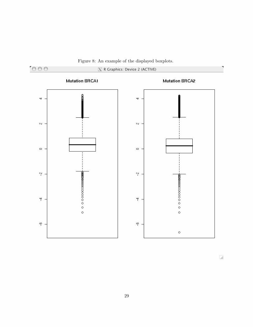
Figure 8: An example of the displayed boxplots.
29
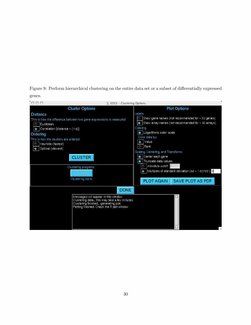
Figure 9: Perform hierarchical clustering on the entire data set or a subset of differentially expressed
genes.
30
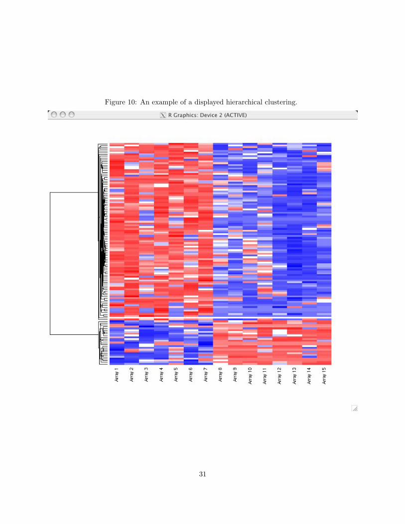
Figure 10: An example of a displayed hierarchical clustering.
31
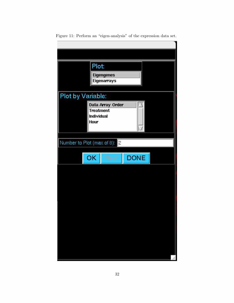
Figure 11: Perform an “eigen-analysis” of the expression data set.
32
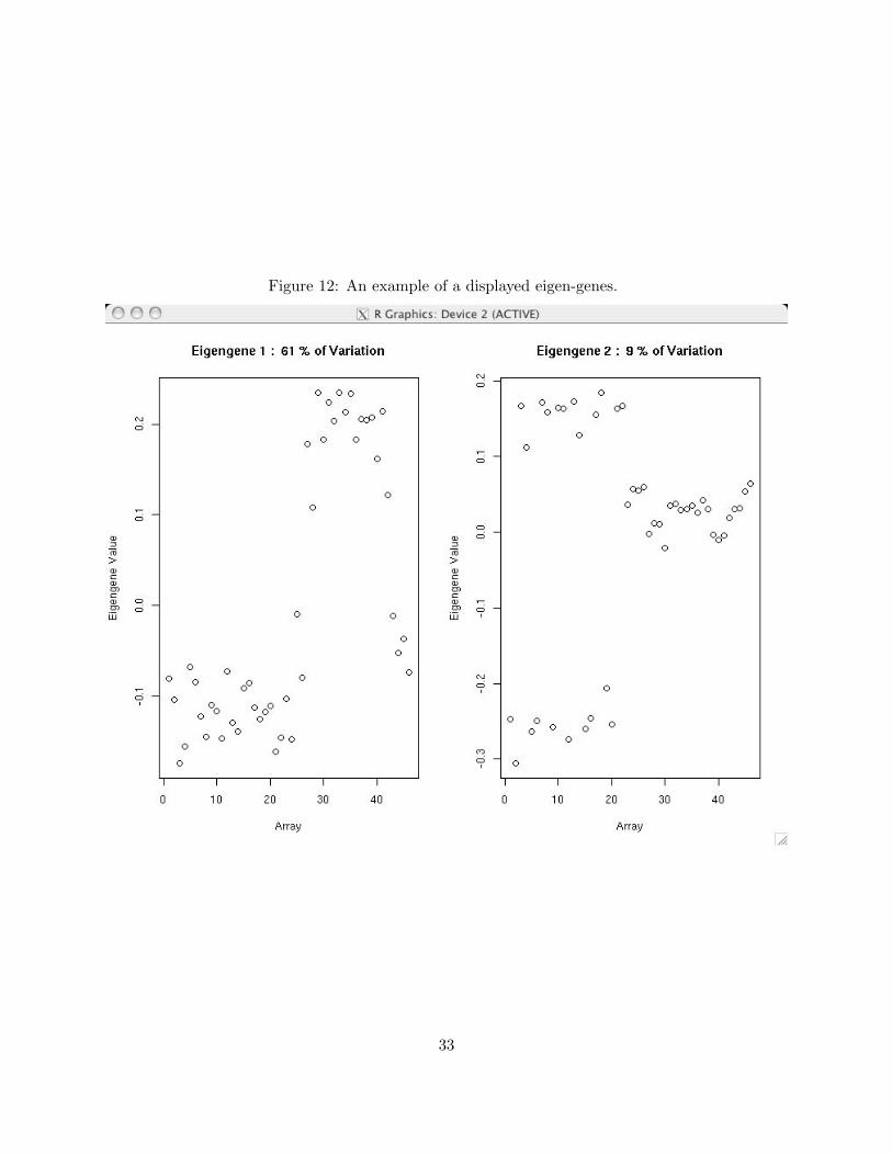
Figure 12: An example of a displayed eigen-genes.
33
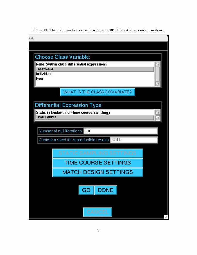
Figure 13: The main window for performing an EDGE differential expression analysis.
34
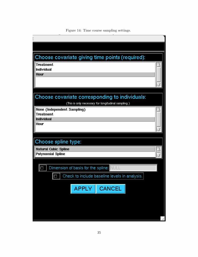
Figure 14: Time course sampling settings.
35
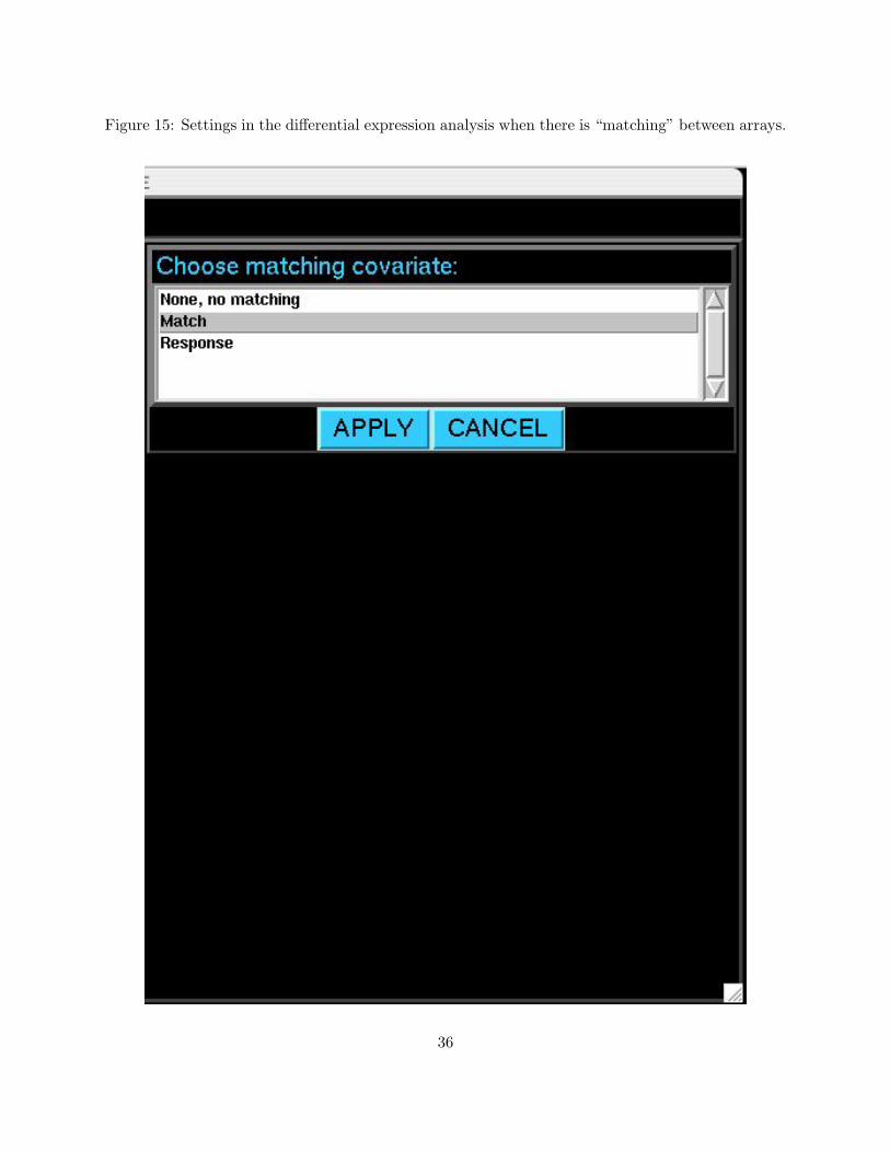
Figure 15: Settings in the differential expression analysis when there is “matching” between arrays.
36
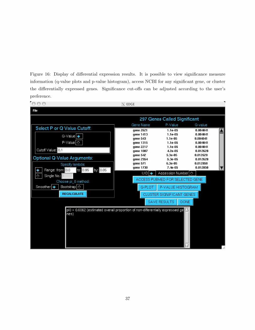
Figure 16: Display of differential expression results. It is possible to view significance measure
information (q-value plots and p-value histogram), access NCBI for any significant gene, or cluster
the differentially expressed genes. Significance cut-offs can be adjusted according to the user’s
preference.
37
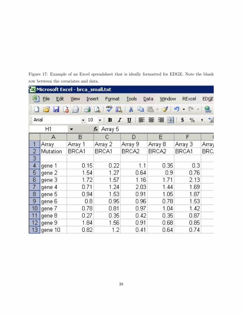
Figure 17: Example of an Excel spreadsheet that is ideally formatted for EDGE. Note the blank
row between the covariates and data.
38