the many faces of marginal analysis - maryland council on ... · *for a perfectly competitive firm,...

The Many Faces of Marginal Analysis

Gary Stone

Winthrop University

“How many of you will…

“How many of you will do all you can to earn an A in my Economics course?”

Coins in an Envelope

Coins in an Envelope

If your marginal benefit is greater than your marginal cost, say “yes.”

If your marginal benefit is less than your marginal cost, say “no.”

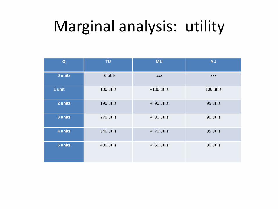
Marginal analysis: utility

Q TU MU AU

0 units 0 utils xxx xxx

1 unit 100 utils +100 utils 100 utils

2 units 190 utils + 90 utils 95 utils




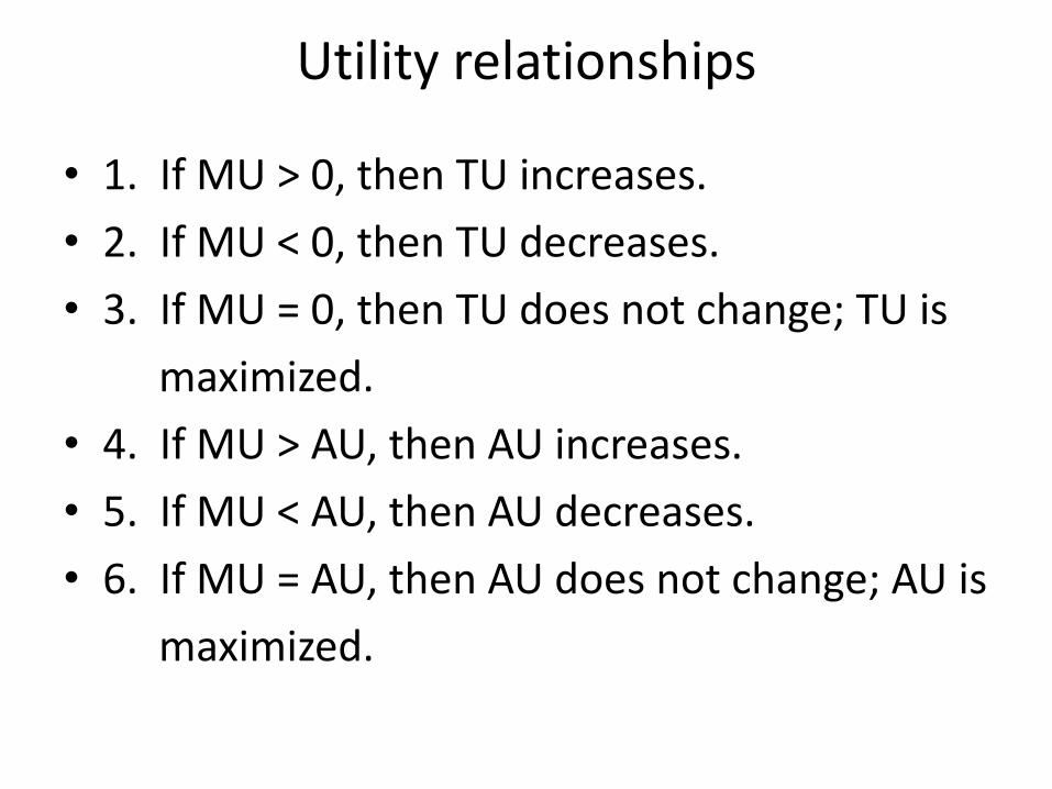
Utility relationships

• 1. If MU > 0, then TU increases.

• 2. If MU < 0, then TU decreases.

• 3. If MU = 0, then TU does not change; TU is

maximized.

• 4. If MU > AU, then AU increases.

• 5. If MU < AU, then AU decreases.

• 6. If MU = AU, then AU does not change; AU is

maximized.

Marginal analysis: productivity

L Q MP AP

0 units 0 units xxx xxx

1 unit 100 units +100 units 100 units

2 units 190 units + 90 units 95 units




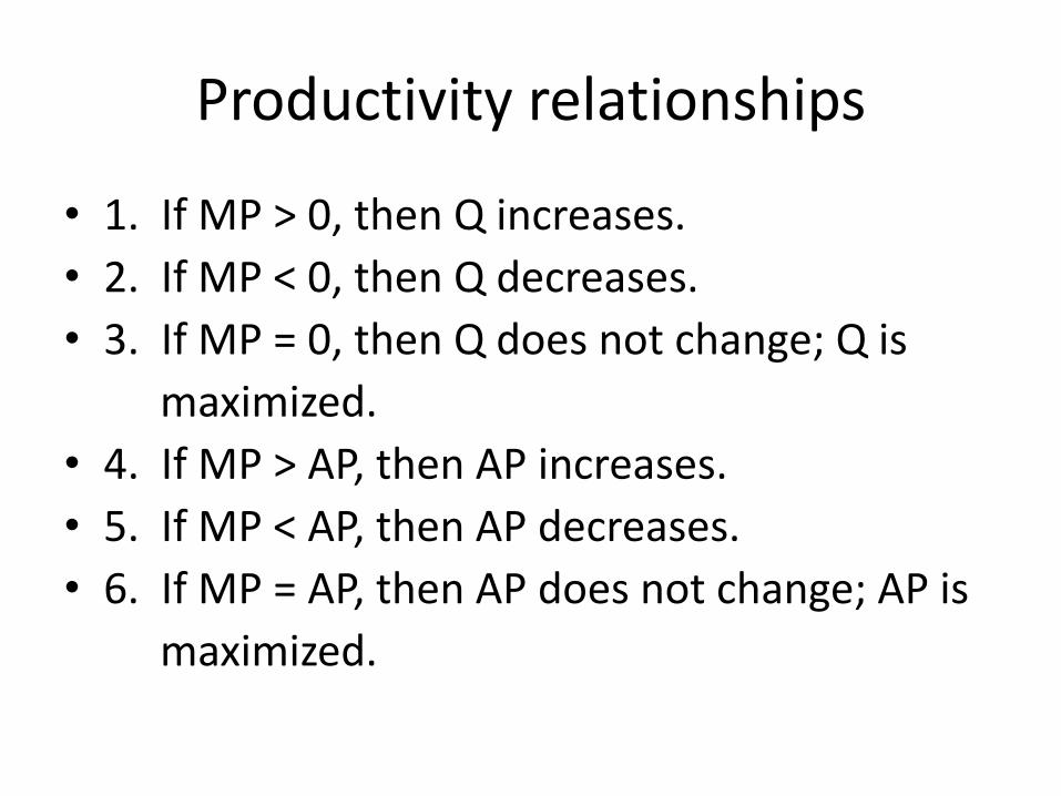
Productivity relationships

• 1. If MP > 0, then Q increases.

• 2. If MP < 0, then Q decreases.

• 3. If MP = 0, then Q does not change; Q is

maximized.

• 4. If MP > AP, then AP increases.

• 5. If MP < AP, then AP decreases.

• 6. If MP = AP, then AP does not change; AP is

maximized.

Marginal analysis: revenue

Q TR MR AR

0 units $ 0 xxx xxx

1 unit $100 +$100 $100

2 units $190 +$ 90 $ 95

3 units $270 +$ 80 $ 90

4 units $340 +$ 70 $ 85

5 units $400 +$ 60 $ 80

Revenue relationships

• 1. If MR > 0, then TR increases. • 2. If MR < 0, then TR decreases. • 3. If MR = 0, then TR does not change; TR is maximized. • 4. If MR > AR, then AR increases.* • 5. If MR < AR, then AR decreases. • 6. If MR = AR, then AR does not change; AR is maximized.* *For a perfectly competitive firm, MR=AR. For a monopoly and for a monopolistically competitive firm, MR<AR. There are no cases in which MR>AR.

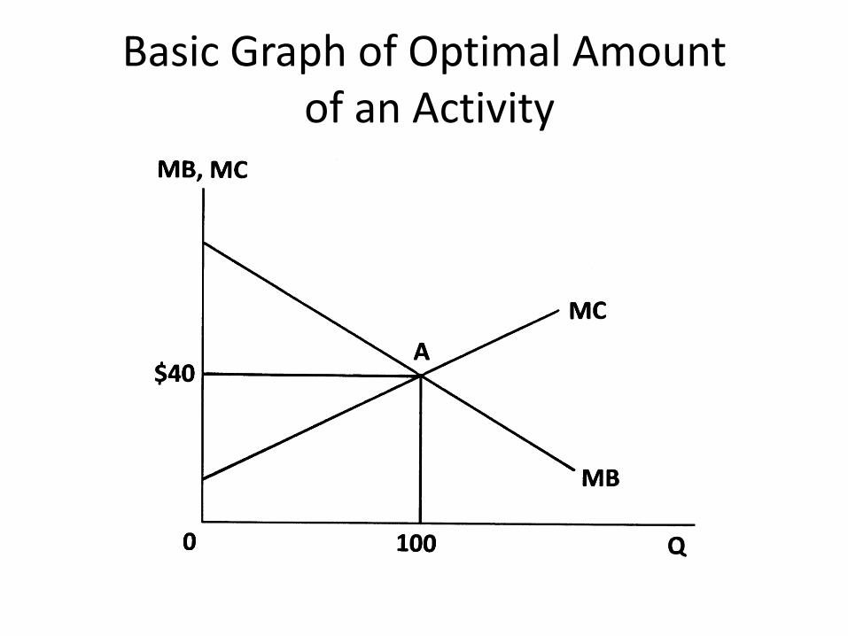
Basic Graph of Optimal Amount of an Activity

Why MB=MC works

The optimal amount of this activity is 100 units. By providing/consuming this quantity, the net total benefit from the activity is maximized. Here is the logic of choosing the quantity at which MB=MC. As shown in this chart, by providing 100 units we are providing all those units which have MB > MC and stopping before providing units which have MB < MC.

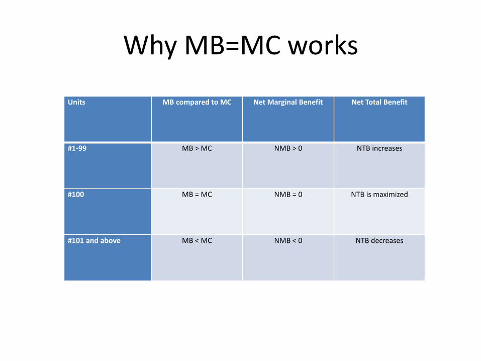
Why MB=MC works

Units MB compared to MC Net Marginal Benefit Net Total Benefit

#1-99 MB > MC NMB > 0 NTB increases

#100 MB = MC NMB = 0 NTB is maximized

#101 and above MB < MC NMB < 0 NTB decreases

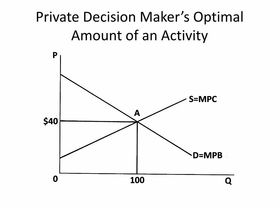
Private Decision Maker’s Optimal Amount of an Activity

Why MPB=MPC works

The optimal amount of this activity is 100 units. By providing/consuming this quantity, the net total benefit from the activity is maximized. Here is the logic of choosing the quantity at which MPB=MPC. As shown in this chart, by providing 100 units we are providing all those units which have MPB > MPC and stopping before providing units which have MPB < MPC.

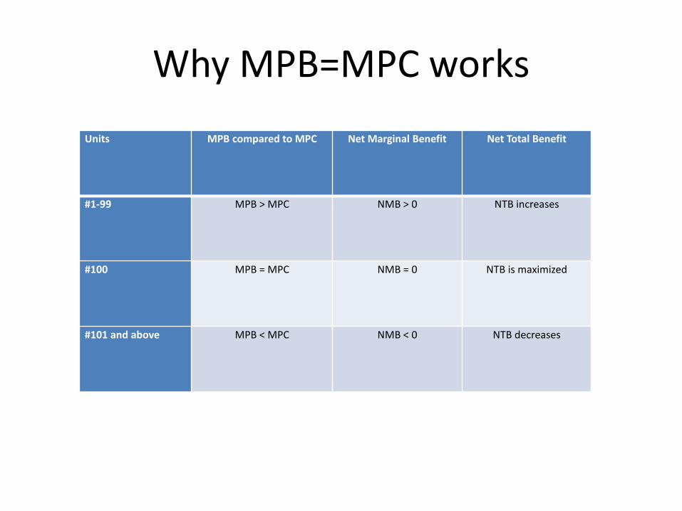
Why MPB=MPC works

Units MPB compared to MPC Net Marginal Benefit Net Total Benefit

#1-99 MPB > MPC NMB > 0 NTB increases

#100 MPB = MPC NMB = 0 NTB is maximized

#101 and above MPB < MPC NMB < 0 NTB decreases

The Socially Optimal Amount of an Activity

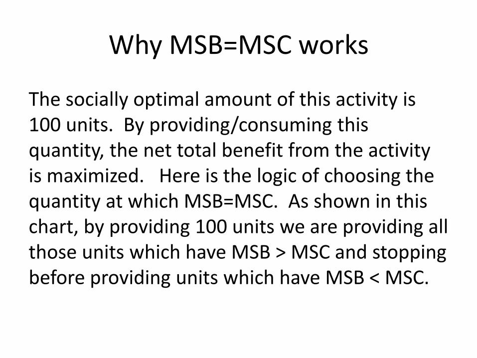
Why MSB=MSC works

The socially optimal amount of this activity is 100 units. By providing/consuming this quantity, the net total benefit from the activity is maximized. Here is the logic of choosing the quantity at which MSB=MSC. As shown in this chart, by providing 100 units we are providing all those units which have MSB > MSC and stopping before providing units which have MSB < MSC.

Why MSB=MSC works

Units MSB compared to MSC Net Marginal Benefit Net Total Benefit

#1-99 MSB > MSC NMB > 0 NTB increases

#100 MSB = MSC NMB = 0 NTB is maximized

#101 and above MSB < MSC NMB < 0 NTB decreases

The Market Quantity as the Socially Optimal Quantity (no externalities)

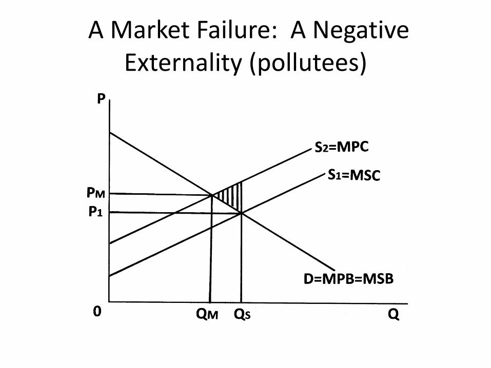
A Market Failure: A Negative Externality (polluters)

A Market Failure: A Negative Externality (polluters)

• When there is no pollution, the market results in the socially optimal quantity QS and the price P1. When some firms decide to stop cleaning their wastes, they reduce their marginal private costs (MPC) which results in an increase in the market supply to S2. This increase in supply results in an increase in market quantity to QM and a reduction in price to PM. The shaded area is the deadweight loss caused by the increased output from QS to QM.

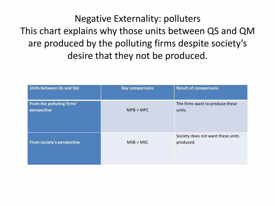
Negative Externality: polluters This chart explains why those units between QS and QM

are produced by the polluting firms despite society’s desire that they not be produced.

Units between QS and QM Key comparisons Result of comparisons

From the polluting firms’

perspective

MPB > MPC

The firms want to produce these

units.

From society’s perspective

MSB < MSC

Society does not want these units

produced.

A Market Failure: A Negative Externality (pollutees)

Negative Externality: pollutees

When there is no pollution, the market results in the socially optimal quantity QS and the price P1. When some firms decide to stop cleaning their wastes, other firms are harmed because they must clean the environment so they can continue to use clean resources (e.g., water from a river). These firms which are negatively impacted by the pollution have an increase in their marginal private costs (MPC) which results in a decrease in the market supply to S2. This decrease in supply results in a decrease in market quantity to QM and an increase in price to PM. The shaded area is the deadweight loss in this market caused by the decreased output from QS to QM pollution.

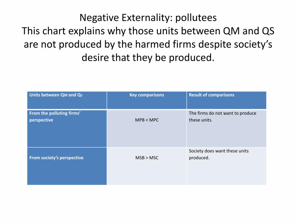
Negative Externality: pollutees This chart explains why those units between QM and QS are not produced by the harmed firms despite society’s

desire that they be produced.

Units between QM and Qs Key comparisons Result of comparisons

From the polluting firms’

perspective

MPB < MPC

The firms do not want to produce

these units.

From society’s perspective

MSB > MSC

Society does want these units

produced.

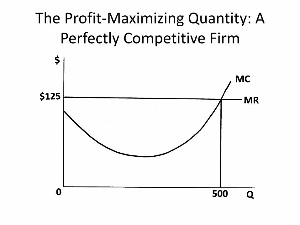
The Profit-Maximizing Quantity: A Perfectly Competitive Firm


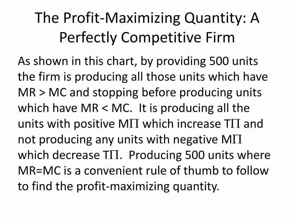
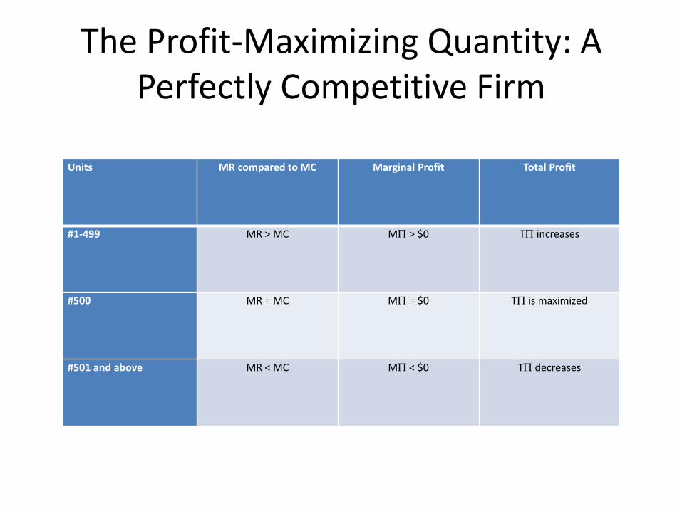
As shown in this chart, by providing 500 units the firm is producing all those units which have MR > MC and stopping before producing units which have MR < MC. It is producing all the units with positive MP which increase TP and not producing any units with negative MP which decrease TP. Producing 500 units where MR=MC is a convenient rule of thumb to follow to find the profit-maximizing quantity.


Units MR compared to MC Marginal Profit Total Profit

#1-499 MR > MC MP > $0 TP increases

#500 MR = MC MP = $0 TP is maximized

#501 and above MR < MC MP < $0 TP decreases

The Profit-Maximizing Quantity: A Monopoly


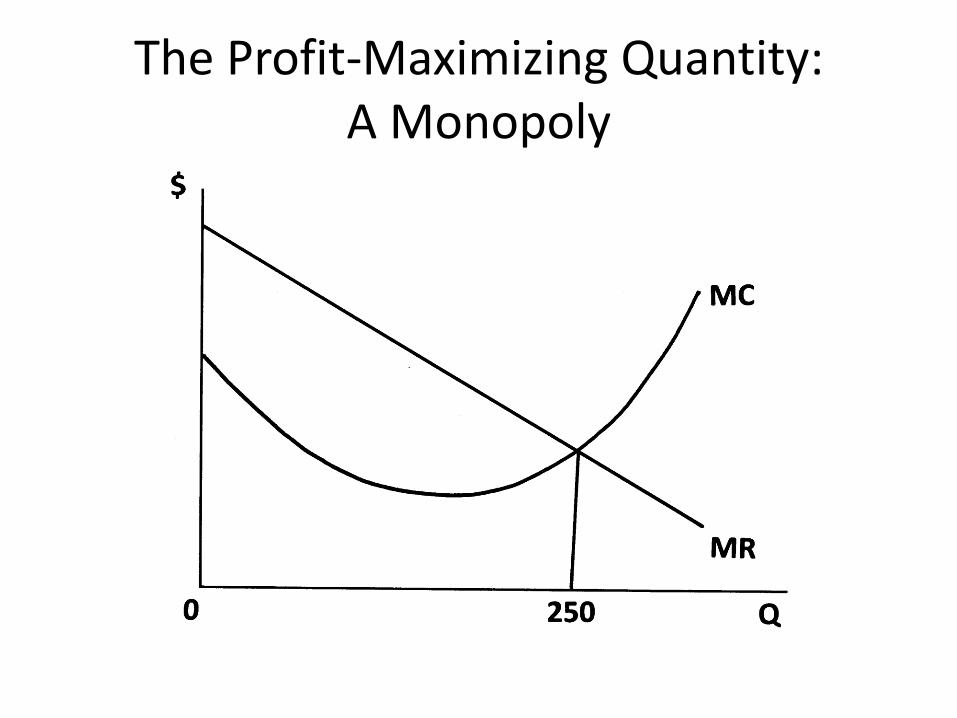
As shown in this chart, by providing 250 units the firm is producing all those units which have MR > MC and stopping before producing units which have MR < MC. It is producing all the units with positive MP which increase TP and not producing any units with negative MP

which decrease TP. Producing 250 units where MR = MC is a convenient rule of thumb to follow to find the profit-maximizing quantity.


Units MR compared to MC Marginal Profit Total Profit

#1-249 MR > MC MP > $0 TP increases

#250 MR = MC MP = $0 TP is maximized

#251 and above MR < MC MP < $0 TP decreases

The Profit-Maximizing Quantity of Labor: A Perfectly Competitive Employer


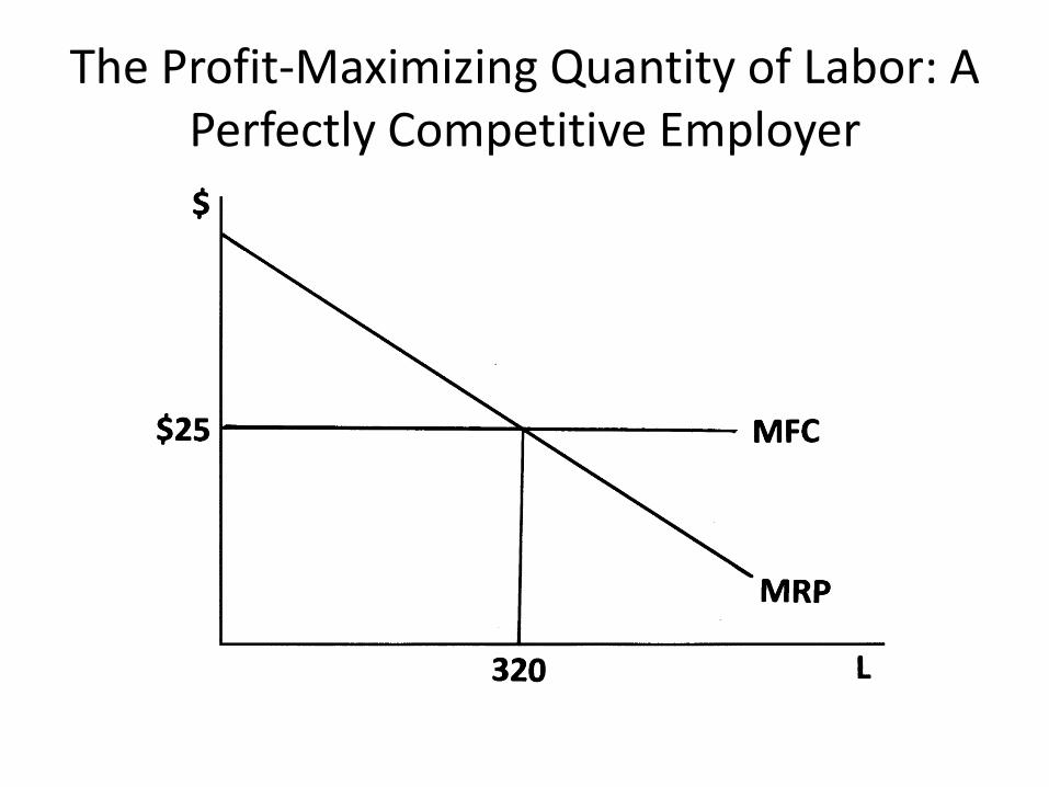
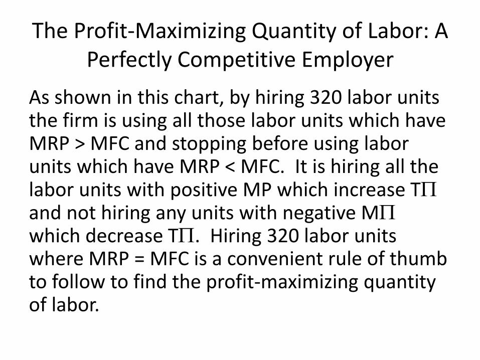
As shown in this chart, by hiring 320 labor units the firm is using all those labor units which have MRP > MFC and stopping before using labor units which have MRP < MFC. It is hiring all the labor units with positive MP which increase TP and not hiring any units with negative MP which decrease TP. Hiring 320 labor units where MRP = MFC is a convenient rule of thumb to follow to find the profit-maximizing quantity of labor.


Labor Units MRP compared to MFC Marginal Profit Total Profit

#1-319 MRP > MFC MP > $0 TP increases

#320 MRP = MFC MP = $0 TP is maximized

#321 and above MRP < MFC MP < $0 TP decreases

The Profit-Maximizing Quantity of Labor: A Monopsonistic Employer


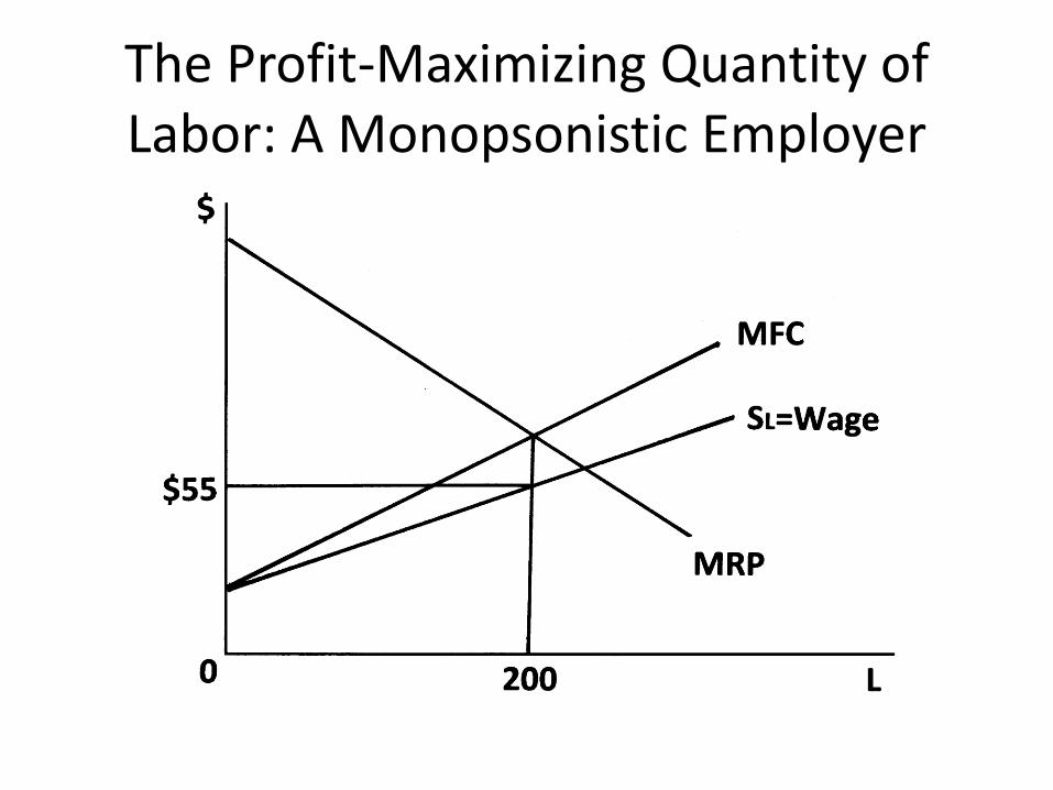
As shown in this chart, by hiring 200 labor units the firm is using all those labor units which have MRP > MFC and stopping before using labor units which have MRP < MFC. It is hiring all the labor units with positive MP which increase TP and not hiring any units with negative MP which decrease TP. Hiring 200 labor units where MRP = MFC is a convenient rule of thumb to follow to find the profit-maximizing quantity of labor.


Labor Units MRP compared to MFC Marginal Profit Total Profit

#1-199 MRP > MFC MP > $0 TP increases

#200 MRP = MFC MP = $0 TP is maximized

#201 and above MRP < MFC MP < $0 TP decreases

The Monopolist's Product Demand Curve is Above its MR Curve

The Monopolist's Product Demand Curve is Above its MR Curve

Quantity Price Total Revenue Marginal Revenue

5 units $40 $150

6 units $28 $168 $18

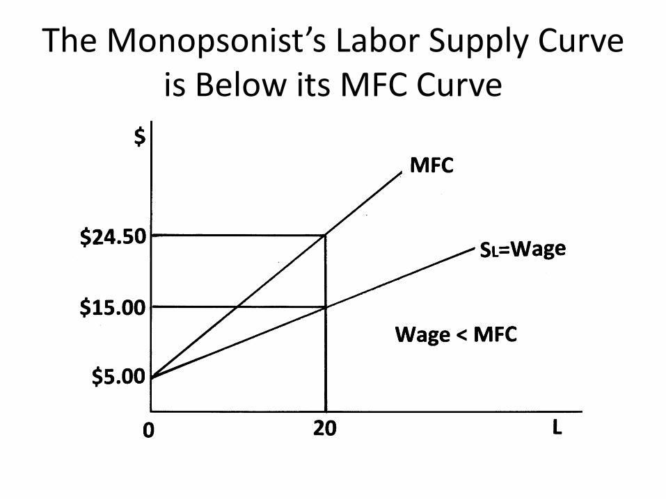
The Monopsonist’s Labor Supply Curve is Below its MFC Curve

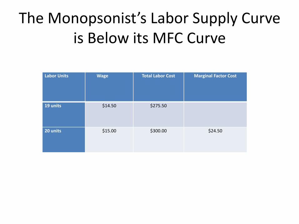
The Monopsonist’s Labor Supply Curve is Below its MFC Curve

Labor Units Wage Total Labor Cost Marginal Factor Cost

19 units $14.50 $275.50

20 units $15.00 $300.00 $24.50

Q* and L* Are Connected!

• The profit-maximizing quantity is Q* where MR=MC.

• The profit-maximizing labor is L* where MRP=MFC.

• The quantity produced by L* is Q*.

One more marginal look-alike

Consumer equilibrium occurs when

MUx = MUy

Px Py

Economic efficiency occurs when

MPL = MPK

PL PK

Bottom line….

Tell your students there really are not that many different things to memorize!

the many faces of marginal analysis - maryland council on ... · *for a perfectly competitive firm,...

Documents