The Map is not the Territory:

Challenges in Extracting Science fromGlobal Simulations

John Lyon

and a host of others

A map is not the territory it represents, but if correct, it has a similar

structure to the territory, which accounts for its usefulness." - Alfred

Korzybski

Outline

• Basic LFM• Science from a code?

– Verification• Is it working properly?

– Validation• How does it compare to observations?

– Scientific Understanding?• flow channels• Kelvin-Helmholtz

• Future directions

MHD equations in LFM

Major Global Codes

Code TVD Order Grid div B Ion.

Elliptic clean

?

Y

Y

Y (strong

?

Y (strong)

Y (strong)

YSpherical ?

2YTanaka

YAMR1?Jahunnen

NCartesian1NWinglee

NCartesian2NOgino

Y Mixed2YMRC

YAMR2YMichigan

Y Stretched4YUCLA (Raeder)

YAdapted8YCISM (LFM)

Design Considerations for LFM

• High resolving power transport• Adapted grid• Div B = 0• Operation in low β, high Alfven speed regime• Integral ionosphere

Spatial Discretization (finite volume)

Conservative Finite Difference Scheme

• State variables are cell centered quantities and we discretize our model equation with numerical fluxes through the cell interfaces

• Scheme is conservative

1 1

2 2

( ( ) ( ) /i i

dUf U f U x

dt

V SUdV Fds

t

Discretization of Linear Advection

• Spatial domain is broken up into cells • Only a few time levels are carried

0// xuvtu

Donor Cell

• A simple first order algorithm

• Maintains monotonic solution

• Linear advection problem clearly shows diffusive character

1

1/ 2 1/ 2

1

n

i

ni i i

n n ni i i

v tu u F F

xv t

u u ux

Second Order

• A simple second order algorithm

• Does not maintain monotonic solution

• Introduces dispersion errors as seen in linear advection example

1

1/ 2 1/ 2

1 1

1 1

2 2

n

i

ni i i

n n n n ni i i i i

v tu u F F

xv t

u u u u ux

• Combines low order and high order fluxes

• Limiter to keep solution monotonic

• Provides nonlinear numeric resistivity and viscosity

1

1/ 2 1/ 2

1/ 2 1 1

1 1

1 1

1 1

2 2

max 0,

1

2

n

i

ni i i

n n n ni i i i i

n n n ni i i i i

n n n ni i i i i

v tu u F F

x

F u u sign u u

u u Bs u u

s sign u u sign u u

Partial Interface Method

TVD switches

• Used to keep numerical solutions from overshoots in regions where they would normally happen

• Idea is to use a dissipative scheme where needed, and elsewhere go with a more accurate ( in sense of Taylor series, say ) scheme

• Leads to a non-linear technique because the solution algorithm itself depends on the local solution

• Addition of diffusion is generally triggered by sharp gradients, just how sharp can be a parameter of the switch

Numerical Order

• Usually describes the accuracy of an interpolation scheme in terms of a Taylor series.– 4th order means that the solution accurately

represents the Taylor series through the 4th order terms

– also can represent a formal convergence rate for non-discontinuous problems

• Not always relevant for problems with shocks and other discontinuities

Treatment of the Magnetic Field• Various approaches can be used to satisify the

constraint that B=0– Projection method

B convection• Modify the MHD equations so that B convects through

the system, allows jumps in Bװ

– Use a magnetic flux conservative scheme that keeps B=0

– Marder Scheme (diffuse divB)

2

'

B

B B

( )0

d

dt

B

Magnetic Flux Conservative Scheme

• Magnetic field placed on center of cell faces

• Electric field is placed at center of cell edges so that

• Cancellation occurs when field components of all six faces are summed up

1 1 1 1 1, , , , , ,

2 2 2 2 2

1 1 1 1, , , ,

2 2 2 2

/

/

x y yi j k i j k i j k

z yi j k i j k

B E E zt

E E y

Computational Grid of the LFM

• Distorted spherical mesh– Places optimal resolution

in regions of a priori interest– Grid is not orthogonal– Logically rectangular nature

allows for easy code development

• Finite Volume Calculation– Requires the calculation

metric quantities• Surface normal direction• Surface Area• Cell Volume

Magnetosphere-Ionosphere Coupling

• Inner boundary of MHD domain is placed between 2-4 RE from the Earth

– High Alfven speeds in this region would impose strong limitations on global step size

– Physical reasonable since MHD not the correct description of the physics occuring within this region

– Covers the high latitude region of the ionosphere (45-90)• Parameters in MHD region are mapped along static dipole

field lines into the ionosphere• Field aligned currents (FACs) and precipitation parameters

are used to solve for ionospheric potential which is mapped back to inner boundary as boundary condition for flow

2

( )

B

Bv

LFMIonospheric Simulation

• 2D Electrostatic Model J||

– J|| determined at magnetospheric BC

• Conductivity Models– Solar EUV ionization

• Creates day/night and winter/summer asymmetries– Auroral Precipitation

• Empirical determination of energetic electron precipitation

• Electric field used for flow at magnetosphere– v = B/B2

Auroral Precipitation Model• Empirical relationships are used to convert MHD

parameters into a characteristic energy and flux of the precipitating electrons– Initial flux and energy

– Parallel Potential drops (Knight relationship)

– Effects of geomagnetic field

– Hall and Pederson Conductance from electron precip. (Hardy)

2 1/ 2o o s oc

1/ 2oRJ

78 7 0

0

o

o

o

o

e

e

o

3/ 2 1/ 2

0.85H2

5 0.45

1 0.0625p p

MHD Simulations• Run a number of cases with Northward IMF

– n=5/cc, v = 400 km/s, Bz = 5 nT

• Chose Northward to avoid complications with activity– still interesting though for

• NBz current position and strength• Relative strength of convection in the four cells• Nature of reconnection above cusp

• All cases have run with N IMF for at least a two hours

Simulations continued

• Have varied the non-linear, TVD, switch sharpness, the spatial order of differencing, and have done one high resolution run for comparison

• standard grid is 50x48x96 => 0.5 Re sorts of resolution at 10 Re

• high resolution is 100x96x128

Simulation Results

• Show three panels for each run– Ionosphere

• FAC is false color surface (lower color bar)• Potential is shown in contours (upper color bar)

– Magntitude of B• Noon-midnight plane shown• vectors are unit vectors in direction of B

– Vx• same plane and vectors

Moderate TVD/ High Spatial Order (8)

High TVD/ 2nd Order

High TVD/4th Order

No TVD/ 8th Order

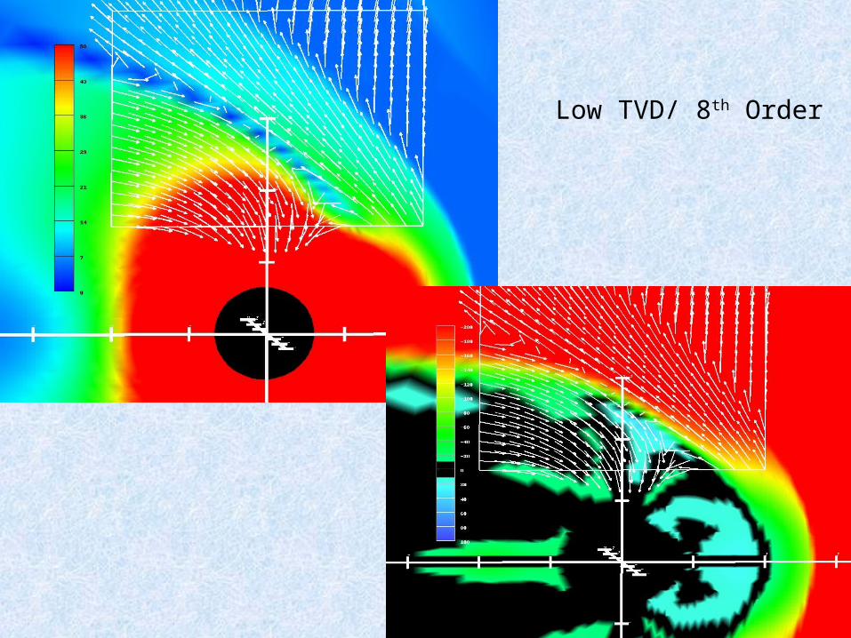
Low TVD/ 8th Order

High TVD/ 8th Order

Doubled Resolution:High TVD/ 8th Order

Simulation Results

• Show three panels for each run– Ionosphere

• FAC is false color surface (lower color bar)• Potential is shown in contours (upper color bar)

– Magntitude of B• Noon-midnight plane shown• vectors are unit vectors in direction of B

– Vx• same plane and vectors

Moderate TVD/ High Spatial Order (8)

High TVD/ 2nd order spatial

High TVD/ 4th Order

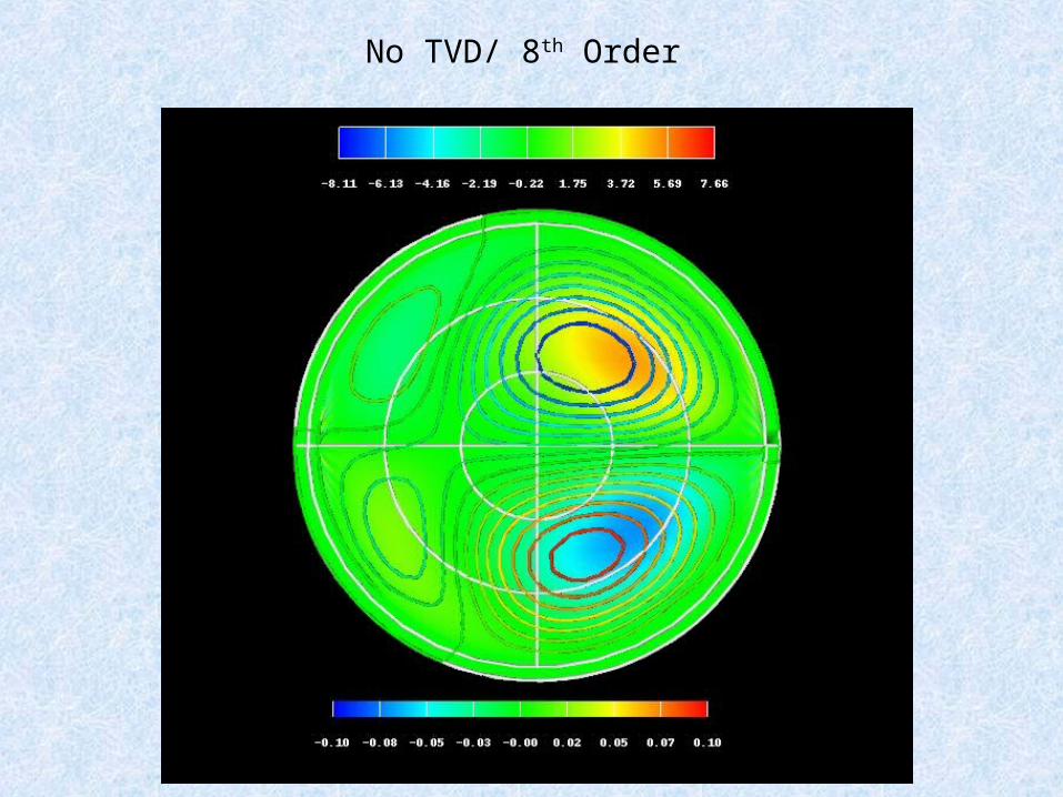
No TVD/ 8th Order

Low TVD/ 8th Order

High TVD/ 8th Order

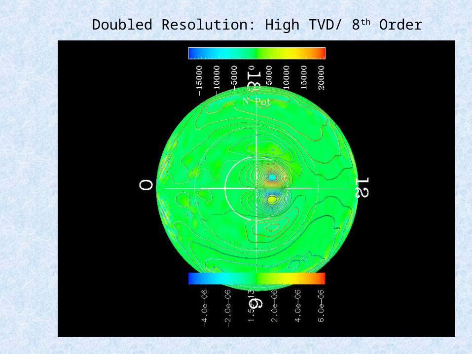
Doubled Resolution: High TVD/ 8th Order

Conclusions• Once you go to at least a moderately

aggressive TVD scheme, the results start to look very similar qualitatively

• Your conclusion as to how similar given simulations are depends on what you look at– |B| shows little difference across all runs

– Vx and the ionospheric structure are more sensitive to the numerics

• The differences, however, are sufficiently large that quantitative comparisons of many quantities will be quite different

Verification?• Pressure for N IMF

Validation

• Major CISM Activity

• Both event and statistical

Comparison with geostationary observations

• ?? agreement for all three components of B

• Resolution improves the results for Bz, in particular

• Dayside works better than nightside– Most likely a ring

current effect

Velocity histogram for tail plasma sheet

For Substorms

Flow Channels

Comparison between Flow channels and BBFs

• Flow channels have properties similar to BBF results reported by Angelopolous

• FWHM of VX profile and

magnitude comparable BBF properties

• Use code to determine if they result from localized reconnection or interchange instability

It is also a good rule not to put

overmuch confidence in the

observational

results that are put forward until they

are confirmed by theory. --

A. Eddington

It is also a good rule not to put

overmuch confidence in the

observational

results that are put forward until they

are confirmed by theory. --

A. Eddington

simulation

Flow channel

• Specific entropy

– Consistent with “bubbles”/interchange

– But still don’t know why and how form

In search of the elusive K-H

• Here it is!

• And we see it in the electric field

• and in the density

• the magnetic connectivity doesn't show rolling

up of magnetic boundary

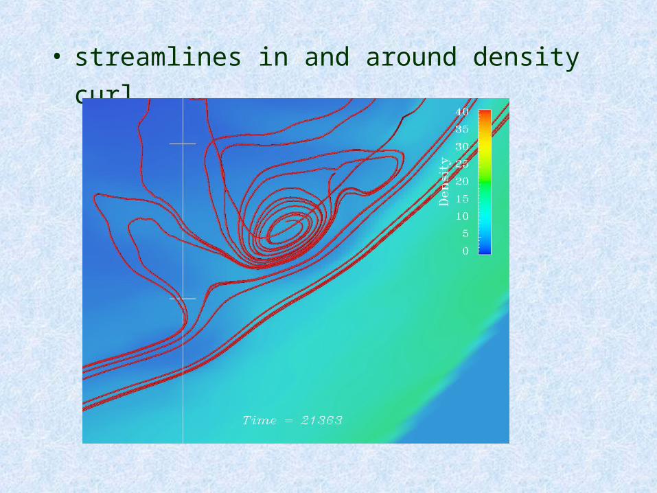
• streamlines in and around density curl

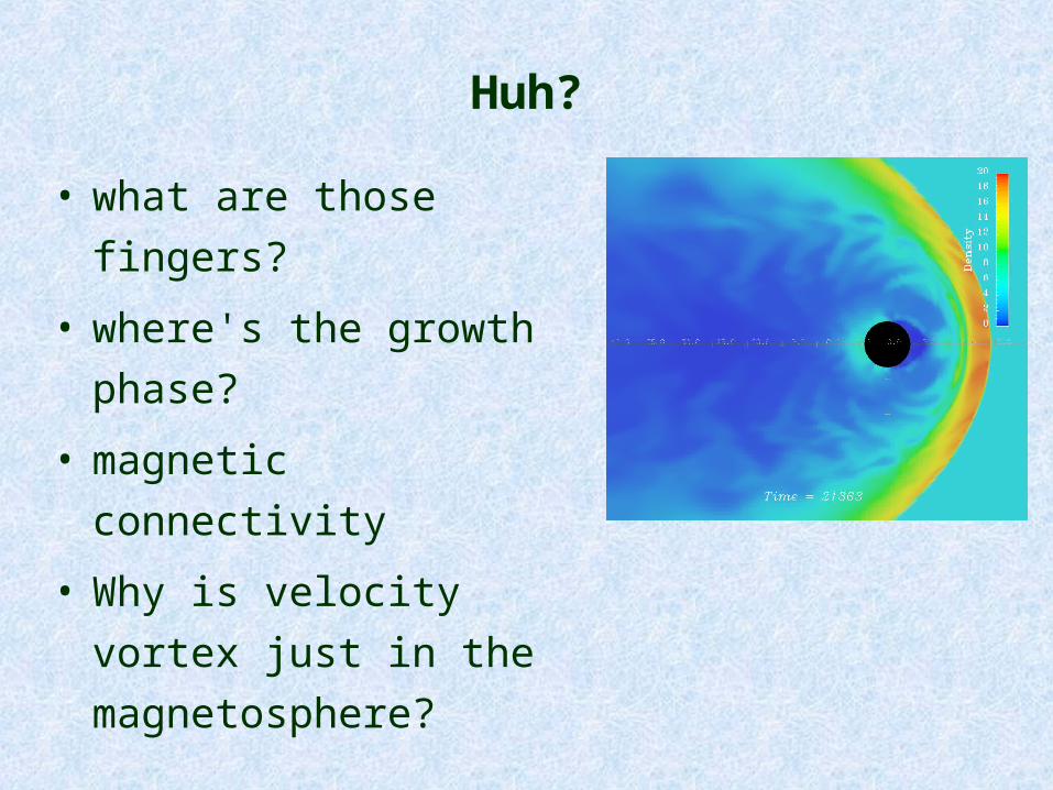
Huh?

• what are those fingers?

• where's the growth

phase?

• magnetic connectivity

• Why is velocity vortex just

in the magnetosphere?

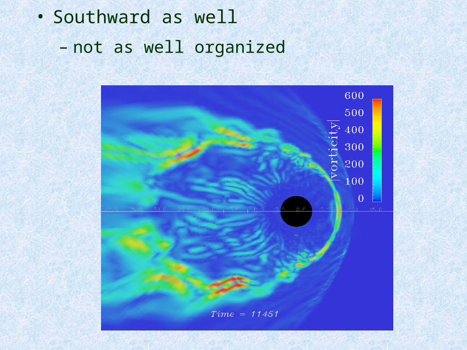
• Southward as well

– not as well organized

• density doesn't show as clear roll-ups

• less internal structure associated with

boundary

• flank reconnection in

vortex?

preliminary conclusions

• seem to have K-H

• depends on IMF direction

• magnetic reconnection/diffusion seems to

maintain a cleaner magnetic boundary

– higher resolution needed?

• sub-solar velocity acceleration in N case

seems to give high growth rate, but where

does it come from?

• vortices seem to lie on magnetosphere side

to do

• diagnostics

– K-H growth rate as finction of position

– careful study of Lagrangian behavior of fluid

and magnetic field

• do they remain coupled? if not, why not?

• higher resolution

Future Code Directions

• Parallelization– “standard” CISM LFM shortly

– MHD code for magnetosphere decoupled from solution of ionosphere/thermosphere

• General purpose capability ( Ogen )

• Multi-fluid Code• Hall Term• Adaptive Grid Capability

– Single grid adaptivity

– Overture multiple grid + AMR

Multi-fluid• currently in OpenMP, moving soon to MPI

Adaptivity

• Lapenta algorithm for Brackbill-Salzmann type adaptivity

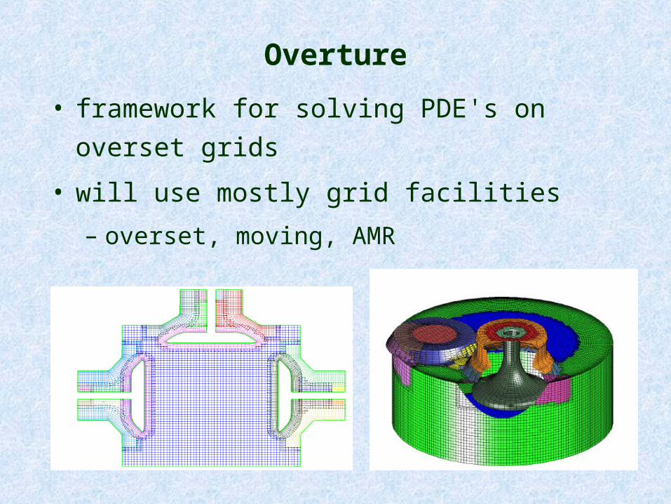
Overture

• framework for solving PDE's on overset grids

• will use mostly grid facilities

– overset, moving, AMR