the mathematical foundations of quantum …the mathematical foundations of quantum indeterminacy...

The mathematical foundations of quantum indeterminacySelf-referential transformations underlyinglogical independence and quantum randomness

Steve Faulkner

29th February 2016

Abstract In 2008, Tomasz Paterek et al published ingenious research, proving that Version 4 4th October 2016Main Edits

� The self-reference proof is now corrected.This had been unfinished.

� Analysis of the Paterek research thesis isgiven enhanced explanation.

� Permanent axioms, introduced earlier:† are explained as being empirically andlogically necessary in isolating the spe-cific logical independence, that hasbeen linked to quantum randomness.† are matched by a corresponding rule forthe conduct of experiments.

� Explanations are generally improved.� Subtitle added.

quantum randomness is the output of measurement experiments, whose input com-mands a logically independent response. Following up on that work, this paperdevelops a full mathematical theory of quantum indeterminacy. I explain how, thePaterek experiments imply, that the measurement of pure eigenstates, and the mea-surement of mixed states, cannot both be isomorphically and faithfully representedby the same single operator. Specifically, unitary representation of pure states iscontradicted by the Paterek experiments. Profoundly, this denies the axiomaticstatus of Quantum Postulates, that state, symmetries are unitary, and observablesHermitian. Here, I show how indeterminacy is the information of transition, frompure states to mixed. I show that the machinery of that transition is unpreventable,logically circular, unitary-generating self-reference: all logically independent. Pro-foundly, this indeterminate system becomes apparent, as a visible feature of themathematics, when unitarity — imposed by Postulate — is given up and aban-doned.

Keywords foundations of quantum theory, quantum mechanics, quantumrandomness, quantum indeterminacy, quantum information, prepared state,measured state, pure states, mixed states, unitary, redundant unitarity, orthogonal,scalar product, inner product, mathematical logic, logical independence, self-reference, logical circularity, mathematical undecidability.

1 Introduction

In Mathematical Physics, validity of a formula stems from its provability — fromPrinciples and Postulates (Axioms). From that standpoint, Mathematical Physicsis a collection of mathematical systems, under a regime of logical dependence.

But, over the past decade, researchers are taking seriously, logical independence,as having impact and significance in Physical Theory [16]. Research includes ex-perimental evidence showing that quantum randomness is rooted in logically inde-pendent, mathematical information [11,12,13]. Logical independence refers to thenull logical connectivity that exists between mathematical formulae, that neitherprove nor disprove one another.

For certain theories, Mathematical Physics must embrace that independence.In the normal way, the system of mathematics should include all provable formulae,derivable from Axioms (whatever they may be); but in addition, the system mustinclude the class of formulae which are not disprovable. This is because the set ofnon-provable, non-disprovable formulae is not empty; and formulae it contains donot contradict, but comply with Axioms. Together, both classes of formulae forma single, consistent theory. Interpretationally, such a system comprises formulaeexpressing cause & effect, and others expressing effect by non-prevention.

For a fundamental example, well-known to Mathematical Logicians [15], I refer tological independence of the imaginary unit.Consider the mathematical system we know as Elementary Algebra. This is ordi-nary school-algebra; the abstracted arithmetic of scalars. In relation to this algebra,

Logical Independence in Physics — Information flow & self-reference in Elementary Algebra.c© Steve Faulkner 2016 E-mail: [email protected]

Steve Faulkner — The Mathematical foundations of quantum indeterminacy 2

the statement:∃x |x2 = −1

is logically independent; it can neither be proved nor disproved by the algebra’saxioms [6]. And yet, existence of any rational number is logically dependent.

Critically, quantum mathematics rests on a foundation of Elementary Algebra.Understanding the origins the of imaginary information, its entry into quantummathematics and its logical relationship with Quantum Postulates is fundamentaland crucial, in revealing Quantum Indeterminacy, as mathematical theory.

In anticipation of readers believing, beyond question, that the imaginary unit isfoundationally axiomatic, I refer to a related article, by this author, providing oneexample contradicting that view. That paper shows that symmetry underpinningwave mechanics of the free particle — the homogeneity symmetry and the CanonicalCommutation Relation deriving from it — has the imaginary unit inserted by themathematician, for other reasons, unrelated to homogeneity [7].

This present paper shows the imaginary unit is not axiomatic, because quantummathematics of pure states does not require it. And also, this paper shows thatentry of the imaginary unit originates, as a requirement, in allowing orthogonalitybetween complimentary systems, necessary in the formation of mixed states.

Quantum indeterminacy is a theoretical concept which must be seen in the contextof empirical quantum randomness; conceived as underlying ontology, explainingquantum randomness. This is ontology, associated with single quantum systems,whose existence we infer, the evidence for which, we witness as randomness instatistics of experiments repeated many times over.

This randomness is not an epistemic randomness. It is not due to information,the detail of which is inaccessible. It is genuine randomness that some regard asfundamentally irreducible.

In classical physics, experiments of chance, such as coin-tossing and dice-throwing,are deterministic, in the sense that, perfect knowledge of the initial conditionswould render outcomes perfectly predictable. This ‘classical randomness’ stemsfrom ignorance of physical information in the initial toss or throw.

In diametrical contrast, in the case of quantum physics, the theorems of Kockenand Specker [10], the inequalities of John Bell [4], and experimental evidence ofAlain Aspect [1,2], all indicate that quantum randomness does not stem from anysuch physical information.

As response, Tomasz Paterek et al provide an explanation in mathematical in-formation. They demonstrate a link between quantum randomness and logical in-dependence in a formal system of Boolean propositions [11,12,13]. In experimentsmeasuring photon polarisation, Paterek et al demonstrate statistics correlating pre-dictable outcomes with logically dependent mathematical propositions, and randomoutcomes with propositions that are logically independent.

Whilst, from the Paterek research, we may reliably infer that the machinery ofquantum randomness does entail logical independence, the fact that this logical in-dependence is seen in a Boolean system, rather obscures any insight. To understandthe workings of quantum randomness, theory must be written exhibiting logical in-dependence in context of standard textbook quantum theory — specifically, in termsof the Pauli algebra su(2).

Here, in this paper, I show what the Paterek Boolean information means for thesystem of Pauli operators. The interesting surprise revealed, is that although everymeasurement of polarisation is representable by the Pauli algebra su (2), only themeasurement of mixed states requires this algebra. Measurement of pure eigenstatesdoes not. For pure states, the unitary component of the Pauli algebra is not involved.

In predictable experiments, where measurement is on pure states, unitarity isshown to be ‘redundant’ — possible but not necessary. And in experiments whoseoutcomes are random, where measurement is on mixed states, unitarity is shownunavoidably necessary. My conclusion is that there is a unitary switch-on in passingfrom pure states to mixed and a unitary switch-off in passing from mixed to pure.

Logically, this regime can be viewed in two ways. It can be viewed as a systemthat is always unitary, but where unitarity switches between possible and necessary:such a possible / necessary system constitutes a modal logic. Or otherwise, it canbe seen as a complete switch between different symmetries, where unitarity is new,


logically independent, extra information required for the transition. To adequatelydescribe the transition between pure and mixed states, either modal logic is needed,or logical independence. The classical logic of true and false is not an option.

The question of where the newly formed unitary information comes from issolved. I show that it has origins in uncaused, unprevented, logically circular self-reference. By uncaused and unprevented, I mean that no information already presentin the system implies nor denies the logically circular self-reference.

In experiments measuring mixed states, whose outcomes are random; in the usualway, the system symmetry is isomorphically and faithfully represented, one-one, bythe (unitary) Pauli matrices:

σx =(

0 11 0

)σy =

(0 −ii 0

)σz =

(1 00 −1

)(1)

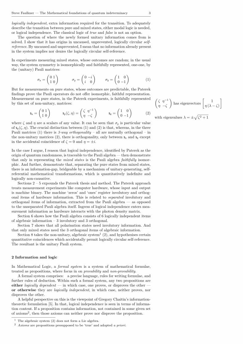
But for measurements on pure states, whose outcomes are predictable, the Paterekfindings prove the Pauli operators do not offer isomorphic, faithful representation.Measurement on pure states, in the Paterek experiments, is faithfully representedby this set of non-unitary, matrices:

(ζ η−1

η −ζ

)has eigenvectors

[1

η (λ− ζ)

]

with eigenvalues λ = ±√ζ2 + 1

sx =(

0 11 0

)sy(ζ, η) =

(ζ η−1

η −ζ

)sz =

(1 00 −1

)(2)

where ζ and η are a scalars of any value. It can be seen that σy is particular valueof sy(ζ, η). The crucial distinction between (1) and (2) is that, whereas, in the threePauli matrices (1) there is 3-way orthogonality – all are mutually orthogonal – inthe non-unitary matrices (2), there is orthogonality, only between sx and sz exceptin the accidental coincidence of ζ = 0 and η = ±i.

In the case I argue, I reason that logical independence, identified by Paterek as theorigin of quantum randomness, is traceable to the Pauli algebra — then demonstratethat only in representing the mixed states is the Pauli algebra faithfully isomor-phic. And further, demonstrate that, separating the pure states from mixed states,there is an information-gap, bridgeable by a mechanism of unitary-generating, self-referential mathematical transformations, which is quantitatively indefinite andlogically non-causative.

Sections 2 – 5 expounds the Paterek thesis and method. The Paterek approachtreats measurement experiments like computer hardware, whose input and outputis machine binary. The machine ‘zeros’ and ‘ones’ register involutory and orthog-onal items of hardware information. This is related to separated involutory andorthogonal items of information, extracted from the Pauli algebra — as opposedto the unseparated Pauli algebra itself. Ingress of logical independence enters mea-surement information as hardware interacts with the photon density matrix.

Section 6 shows how the Pauli algebra consists of 6 logically independent itemsof algebraic information – 3 involutory and 3 orthogonal.

Section 7 shows that all polarisation states need involutory information. Andthat only mixed states need the 3 orthogonal items of algebraic information.

Section 8 takes the non-unitary, algebraic system1 (2), and hypothesises certainquantitative coincidences which accidentally permit logically circular self-reference.The resultant is the unitary Pauli system.

2 Information and logic

In Mathematical Logic, a formal system is a system of mathematical formulae,treated as propositions, where focus in on provability and non-provability.

A formal system comprises: a precise language, rules for writing formulae, andfurther rules of deduction. Within such a formal system, any two propositions areeither logically dependent — in which case, one proves, or disproves the other —or otherwise they are logically independent, in which case, neither proves, nordisproves the other.

A helpful perspective on this is the viewpoint of Gregory Chaitin’s information-theoretic formulation [5]. In that, logical independence is seen in terms of informa-tion content. If a proposition contains information, not contained in some given setof axioms2, then those axioms can neither prove nor disprove the proposition.

1 The algebraic system (2) does not form a Lie algebra.2 Axioms are propositions presupposed to be ‘true’ and adopted a priori.


Edward Russell Stabler explains logical independence in the following terms.A formal system is a postulate-theorem structure; the term postulate being syn-onymous with axiom. In this structure, there is discrimination, separating assumedfrom provable statements. Any statement labelled as a postulate which is capableof being proved from other postulates should be relabelled as a theorem. And ifretained as a postulate, it is logically superfluous and redundant [15]. If incapableof being proved or disproved from other postulates, it is logically independent.

Central to the formal system used in the Paterek et al research are these Booleanfunctions of a binary argument:

x ∈ {0, 1} 7→ f (x) ∈ {0, 1}

Typical propositions, stemming from those functions, are these:

f (0) = 0 f (1) = 0 f (0) = f (1)f (0) = 1 f (1) = 1 f (0) 6= f (1) (3)

Such propositions are items of information, taken as being openly true or openlyfalse. Our interest lies, not so much, in their truth or falsity, but in, which statementsprove which, which disprove which, and which do neither. In other words, whichare logically dependent and which are logically independent.

As illustration, if f (0) = 0 were considered to be true, the statement f (0) = 1would be proved false. More simply, we could say: f (0) = 0 disproves f (0) = 1,and accordingly, f (0) = 1 is logically dependent on f (0) = 0.

On the other hand, again, if f (0) = 0 were considered to be true, that would notprove, or disprove f (1) = 0. We could say: f (0) = 0 neither proves, nor disprovef (1) = 0, and accordingly, f (0) = 0 and f (1) = 0 are logically independent.

Over and above the propositions in (3), I introduce permanent axioms, which Pa-terek et al take for granted, but do not state. They are:

f (0) = 0 ⇒ f (1) = 1 f (1) = 0 ⇒ f (0) = 1 (4)

These prohibit the combination f (0) = 0, f (1) = 0. More is said about this inSection 5.

3 The Paterek et al experiments

The Paterek et al research involves polarised photons as information carriers throughmeasurement experiments. The experiment hardware consists of a sequence of threesegments, which I denote: State preparation, Black box and Measurement. These pre-pare, then transform, then measure polarisation states. The orientational configu-ration of the three segments is the experiment’s input data. This is read from anX–Y–Z reference system fixed to the hardware. Outcome states of polarisation arethe experiment’s output data. Experiments were performed, very many times, andstatistics of outcomes gathered. The configuration input, is related to whether theexperiment’s output is random or predictable.

1. State preparationPhotons prepared, either as |z+〉, |x+〉 or |y+〉 eigenstates, by filtering, directlyafter one of these Pauli transformations:(a) σz, aligned with the Z axis.(b) σx, aligned with the X axis.(c) σy, aligned with the Y axis.

2. Black boxThe prepared eigenstates are altered through one of these Pauli transformations:(a) σz, aligning states with the Z axis,(b) σx aligning states with the X axis,(c) σy aligning states with the Y axis.

3. MeasurementMeasurement is performed, by detecting photon capture, directly after one ofthese Pauli transformations:(a) σz, aligned with the Z axis.(b) σx, aligned with the X axis.


(c) σy, aligned with the Y axis.Thus, there are 27 possible experiments. In practice, nine are necessary. Results aresufficiently demonstrated by always keeping the State preparation orientation, setat the same alignment as the Measurement orientation. The fact that Measurementcopies the State preparation orientation means the full hardware configuration canbe encoded, taking orientations of the Black box and Measurement segments, only.These encodings come in the form of Boolean ‘4-sequences’ and ‘quad-products’introduced below.

Within experiments, there exist two classes of orientational information. The moreobvious is segment alignment; this is the orientation of individual hardware seg-ments with respect to the X–Y–Z reference system. Normally, in standard theory,segment alignment would be represented as Pauli information, through the σx, σy,σz operators. In the Paterek et al research, alignment information is fully conveyedin two bits, through three Boolean pairs — (0, 1), (1, 0), (1, 1).

The less obvious class of information, I refer to as orthogonality index. Thisis the degree of orthogonality between one hardware segment and the next —either orthogonal, or not orthogonal. Orthogonality index is conveyed through theexperiment, as information propagated in the density matrix.

4 Boolean pairs and 4-sequences

In their treatment of the mathematics, Paterek et al represent their experimentconfigurations, using sequences of the three Boolean pairs — (0, 1), (1, 0), (1, 1).Information held in these pairs is taken directly from the indices, in the productσixσ

jz , where i and j are interpreted as integers, modulo 2. Thus:

σz = σ0xσ

1z σx = σ1

xσ0z −iσy = σ1

xσ1z (5)

By way of these three formulae, Boolean pairs (0, 1), (1, 0), (1, 1) are linked to theoperators: σz, σx, σy.

The idea is that the whole information of any Pauli operator can be encodedthrough different arrangements of σx and σz — just two of the Pauli operators. Theprecise structure of that encoding is key to accessing and revealing the informationthat constitutes indeterminacy.

Stringing together sequences of Pauli operators, to form ‘quad-products’, invokescorresponding Boolean ‘4-sequences’. These represent orientational information,linking two consecutive segments of the experiment hardware. Examples are:

σzσz = σ0xσ

1zσ

0xσ

1z → (0, 1) (0, 1) (6)

σxσz = σ1xσ

0zσ

0xσ

1z → (1, 0) (0, 1) (7)

−iσyσz = σ1xσ

1zσ

0xσ

1z → (1, 1) (0, 1) (8)

These can be used to represent the action of the State preparation followed by theaction of the Black box; OR, the action of the Black box followed by the action ofthe Measurement.

Consider a specific experiment where the action of the State preparation is en-coded thus:

σmx σnz → (m,n)

where the action of the Black box is encoded thus:

σf(0)x σf(1)

z → (f (0) , f (1)) (9)

where f (0) and f (1) are the Boolean functions relating to propositions written in(3); and the action of the Measurement is encoded thus: Variables p and q are not used by Paterek et al.

I introduce them for the sake of completeness.σpxσ

qz → (p, q)

In this experiment, the joint action for the State preparation and Black box is en-coded in the quad-product and 4-sequence:

σfin(0)x σfin(1)

z σmx σnz → (fin (0) , fin (1)) (m,n)

And the joint action for the Black box and Measurement is encoded in the quad-product and 4-sequence:

σpxσqzσ

fex(0)x σfex(1)

z → (p, q) (fex (0) , fex (1))


5 Logical independence from the Boolean viewpoint

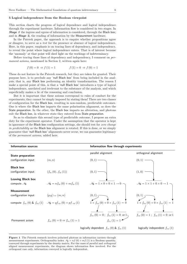
This section charts the progress of logical dependence and logical independencethrough the experiment hardware. Information flow is considered in two stages. InStage 1 the ingress and egress of information is considered, through the Black box;and in Stage 2, the reading of information by the Measurement hardware.

In the Paterek paper, the approach is to enquire whether propositions agreeor disagree, to serve as a test for the presence or absence of logical independence.Here, in this paper, emphasis is on tracing lines of dependency, and independency,to reveal the point where logical independence enters. That is of interest becausethe ‘anomaly’ at that point will shed light on the workings of indeterminacy.

Before tracing those lines of dependency and independency, I comment on per-manent axioms, mentioned in Section 2, written again here:

f (0) = 0 ⇒ f (1) = 1 f (1) = 0 ⇒ f (0) = 1

These do not feature in the Paterek research, but they are taken for granted. Theirpurpose here, is to preclude any ‘null Black box’ from being included in the anal-ysis; that is, any Black box performing an identity transformation. The reason Imake a special point of this, is that a ‘null Black box’ introduces a type of logicalindependence, unrelated and irrelevant to the substance of the analysis, and whichsuperficially makes a lie of the reasoning and conclusion.

But it is important that these axioms correspond to rules of conduct for theexperiments; they cannot be simply imposed by stating them! There are two classesof configuration for the Black box, resulting in non-random, predictable outcomes.One is where the Black box imparts the same polarisation alignment, as does theState preparation. In the other, the Black box imparts no alteration, and photonsexit the Black box, in whatever state they entered from State preparation.

So as to eliminate this second type of predictable outcome, I propose an extraduty for the experiment operator. Under the assumption that the operator is keptin ignorance of the Black box configuration settings, she should test for zero changein predictability as the Black box alignment is rotated. If this is done, or we simplyguarantee that ‘null Black box’ alignments never occur, we can guarantee legitimacyof the permanent axioms, added here.

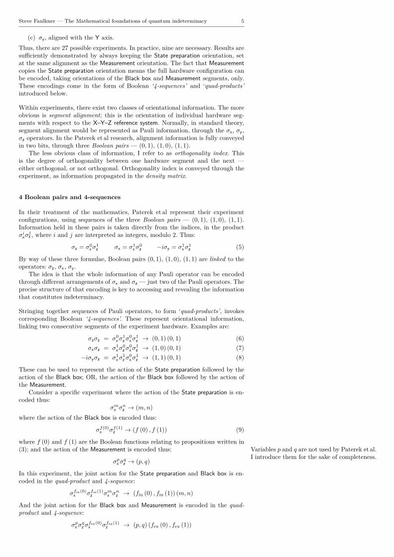
Information sources

parallel alignment orthogonal alignmentState preparation

(m,n) (0, 1) (0, 1)

Black box(fin (0) , fin (1)) (0, 1) (1, 0)

Leaving Black boxcompute NB NB = nfin (0) + mfin (1)

Measurement(0, 1) (0, 1)

compute NB = qf ex (0) + pf ex (1) 1

Permanent axiom fex (0) = 0 ⇒ fex (1) fex (1) = 1

fex (0) = 1 ; fex (1) = 0 or 1

logically independent fex (1)

& fex (1)fex (0)

Information f ow through experimentsl

configuration input

configuration input

configuration input

(p,q ) (m,n)=

NB = 1 × 0 + 0 × 1 → 0 NB = 1 × 1 + 0 × 0 → 1

× fex (0) + 0 × fex (1) 0 1 × fex (0) + 0 × fex (1) 1

fex (0) = 0 ; fex (1) = 0 or 1

= =

& fex (1)fex (0)logically dependent

= 1

Figure 1 The Paterek research involves polarised photons as information carriers throughmeasurement experiments. Orthogonality index NB = nf (0) + mf (1) is a Boolean quantity,conveyed through experiments by the density matrix. For the cases of parallel and orthogonalaligned measurement experiments, the diagram shows information flow involved. For theorthogonal case only, information conveyed is logically independent.


Stage 1 Boolean pairs, representing X–Y–Z information, from State preparationand Black box, feed into the density matrix.

The propagation of information, that encodes, whether states are mixed or pure,is conveyed in the density matrix. On entry into the Black box, the input densitymatrix, is:

ρ = 12 [1 + λmni

mnσmx σnz ]

with λ = ±1. Under the action of the Black box the density matrix evolves to:

UρU† = 12

[1 + λmn (−1)nfin(0)+mfin(1)

imnσmx σnz

]The index, on the factor (−1)nfin(0)+mfin(1), I call the orthogonality index and giveit the label NB, thus:

NB = nfin (0) +mfin (1)

The suffix B stands for ‘leaving the Black box’. This is just downstream of the Blackbox; but upstream of any interference from Measurement. Depending on whetherthe Black box imparts orthogonal information, the value of NB is either 0 or 1. Allsums are taken modulo 2. Incidental: when alignment is parallel, NB = 0

and consequently ρ = UρU†, so there is noevolved change in ρ.NB = nfin (0) +mfin (1) = 0 zero orthogonality imparted by the Black box

NB = nfin (0) +mfin (1) = 1 unit orthogonality imparted by the Black box

Leaving the Black box, NB has a definite, deterministic value, logically dependentlycomputed from (m,n) and (fin (0) , fin (1)). That determination can be thought ofas an information process where (m,n) and (fin (0) , fin (1)) are copied from theState preparation and Black box, then given as input to nfin (0) + mfin (1), fromwhich NB is computed, as output.

Stage 2 Measurement attempts to read the Black box X–Y–Z information.Now comes the interaction between NB and the Measurement hardware. By now,values of fin (0) and fin (1) are either lost or upstream and inaccessible. The densitymatrix conveys NB, not fin (0) and fin (1).

Leaving the Black box, the definite, deterministic value NB, continues its propa-gation through the experiment, to be read as input, into theMeasurement hardware.But the Measurement hardware will have the awkward job of attempting a compu-tation in the ‘backwards’ sense, which will present a problem of computability.

Once the Measurement hardware knows the value NB, given the Measurementorientation, set by

σpxσqz → (p, q)

the Measurement hardware attempts to compute fout (0) and fout (1), from

NB = qfex (0) + pfex (1)

However, fex (0) and fex (1) are not both determinable from NB and (p, q), because,one or the other of fex (0) and fex (1), will be logically independent.

To demonstrate the above, it is sufficient to set the Measurement configuration(p, q) to the same basis (m,n), set for the State preparation. Figure 1 shows theflow of information schematically, comparing the straight-through, parallel alignedexperiment, against the orthogonal experiment configuration.

6 Information content of the Pauli algebra

It is instructive to review the information content of the Pauli algebra, or moresignificantly, the information implied in the formula: −iσy = σ1

xσ1z ; or rather more

strictly, asserted in this abstract formulae:

−ib = ac (10)

That review means going through the process of constructing (10), from scratch,and noting all information needed. The procedure I give is an adaption of a proofgiven by W E Baylis, J Huschilt and Jiansu Wei [3]. This proof possibly originates from a paper by

David Hestenes [9].


The Pauli algebra is a Lie algebra; and hence, is a linear vector space. Therefore, Ibegin with information inherited from the vector space axioms, and then add otherinformation peculiar to the Pauli Lie algebra, su(2).Closure: For any two vectors u and v, there exists a vector w such that

w = u + v

Identities: There exist additive and multiplicative identities, 0 and 1. For anyarbitrary vector v:

v1 = 1v = v (11)v + 0 = 0 + v = v (12)

v0 = 0v = 0 (13)Additive inverse: For any arbitrary vector v, there exists an additive inverse −vsuch that

(−v) + v = 0 (14)Scaling: For any arbitrary vector v, and any scalar a, there exists a vector u suchthat

u = av (15)Products: A feature of Lie algebras is that, between any two arbitrary vectors, uand v, there exist products uv and vu. Commutators of these products (Lie brackets)are members of the vector space.Dimension: Assume a 3 dimensional vector space, with independent basis a, b, c.

The six items of information

Involutory information: Assume all three basis vectors are involutory. Thus:aa = 1 a involutory (16)bb = 1 b involutory (17)cc = 1 c involutory (18)

Orthogonal information: Assume products between basis vectors are orthogonal.Thus:

ab + ba = 0 ab orthogonal (19)bc + cb = 0 bc orthogonal (20)ca + ac = 0 ca orthogonal (21)

Bringing items of information together, the Pauli algebra is constructed thus:bc + cb = 0 by (20) , bc orthogonalb + cbc = 0 by (18) , c involutory

ba + cbca = 0 by (13) (22)And similarly:

ca + ac = 0 by (21) , ca orthogonalcac + a = 0 by (18) , c involutory

cacb + ab = 0 by (13) (23)Adding (23) and (22) gives:

cacb + ab + ba + cbca = 0

cacb + cbca = 0 by (19) , ab orthogonalacb + bca = 0 by (18) , c involutoryacba + bc = 0 by (16) , a involutoryacbac + b = 0 by (18) , c involutory

acbacb + 1 = 0 by (17) , b involutory(acb)2 = − 1 by (14)(acb)2 = (−1) 1

acb = ± i1ac = ± ib by (17) , b involutory (24)


And a couple of extra steps gives the Pauli algebra:

ca = ∓ ib by (24) , a, b, c involutory (25)ac− ca = ± 2ib by (24) & (25) (26)

The six formulae (16) – (21) constitute six items of logically independent infor-mation. They are logically independent because none can be proved nor disprovedfrom the others. All six are needed in proving ac = ±ib.

The ‘3-way orthogonality’ resulting from (19), (20) and (21) implies complexunitarity.

7 Logical independence from the viewpoint of symmetry

Quantitatively, standard Pauli theory is superbly successful. But, in terms of rep-resenting the logic of experiments, it would seem the Paterek Boolean system is animprovement. Accepting that as fact, the Boolean system must be traced throughfor information that standard theory misses.

The Paterek research shows that mathematics encoding the measurement of mixedstates has logically independent structure; and that the measurement of pure statesdoes not. And therefore, any mathematical structure faithfully3 representing the Faithful representation is one-one, isomorphic

representation.

Note that(

0 η−1

η 0

)and

(0 −ii 0

)cannot

be isomorphic because only one of them is amember of the unitary group.

measurement of mixed states cannot faithfully represent pure eigenstates, also.For the faithful representation of pure, and of mixed states, two structures areneeded which are not mutually isomorphic: meaning that no one, single mathemat-ical structure can be isomorphic with every polarisation measurement experiment.This contradicts standard theory, where the Pauli algebra is understood to repre-sent every measurement configuration.

Consequently, the Paterek paper establishes, that measurement of arbitrarilyprepared polarised photons, cannot, in general, be isomorphically represented byany single, exclusive, mathematical structure. Specifically, the Pauli algebra cannotbe relied upon as a general theory, isomorphically representing every configurationof measurement experiment. Instead, measurement aligned parallel to the preparedstate – and – measurement aligned orthogonal against it, are separately representedby distinct mathematical structures, not isomorphic with one another.

Having said all the above, quantitatively, the Pauli theory does work. Resolutionto this quantitative versus logical dichotomy, as will be seen, is in the fact that oneof those distinct mathematical structures agrees with the other, but the other doesnot agree with the one.

The above is helpful news. Of course, we take for granted the fact that individualexperiments are independent of one another. But extra and further to that, theabove tells us, experiments are independent, to the extent, that algebra for oneexperiment does not extrapolate to all others. All Pauli experiments do not shareone same algebraic environment.

In practice, this means the formula (8) does not confer existence of σy uponthe formulae (6). Nor does (8) confer its value of σz upon (6). Et cetera. We mustregard all such formulae, entailing the Pauli quad-products, as individual constructsof information, in isolation from one another, without passing information betweenthem.

The Paterek findings rely on a logical isomorphism, linking the Boolean system withPauli experiments. That isomorphism is a one – one correspondence that connectsthe logic of experiments with the logic of the Boolean system. The Paterek paperremarks on this logical isomorphism in its conclusion.

In contrast, the Pauli system lacks that one – one logical correspondence withexperiment. The position is that the Pauli system faithfully represents experimentsquantitatively whilst the Boolean system faithfully represents experiments logically.In order that the Pauli system should be logical also, it must connect logically,one – one, with Pauli experiments. That means Pauli experiments must connectlogically, one – one, with the Boolean system (as they do); and then in turn, theBoolean system must connect logically, one – one, with the Pauli system. Thus:

Pauli system � Boolean system � Pauli experiments

3


To approach this, we must examine the exact nature of the link relating the Pauliand Boolean systems to see where logical correspondence between them currentlyfails.

Readers of the Paterek paper might infer that there is one – one correspondencelinking the Pauli products with Boolean pairs. The actual picture is one –way.Implication is only directed from the Pauli products, to the Boolean pairs, in thesense of the arrows shown here:

σz = σ0xσ

1z −→ (0, 1) σx = σ1

xσ0z −→ (1, 0) −iσy = σ1

xσ1z −→ (1, 1) (27)

If the Pauli system were to connect logically, one – one, with the Boolean system, wewould witness a backwards implication, also, in the sense of these reverse arrows:

σz = σ0xσ

1z ←− (0, 1) σx = σ1

xσ0z ←− (1, 0) −iσy = σ1

xσ1z ←− (1, 1) (28)

But, as they stand, the formulae in (28) are invalid. Generally, the Boolean pairsdo not imply the Pauli operators. They invoke operators that are not necessarilyPaulian; they invoke operators belonging to some wider system. They do not forma Lie algebra. The Pauli operators are merely the special case that happens to beunitary. And so, we must either abandon the backwards implication — but thisis implicit in the Paterek findings — or accept the replacement of Pauli operatorswith operators that maintain backwards validity.

The situation is made clearer when all Pauli notation is dropped and replaced byabstract symbols c, a, b. Formulae can then be seen for the information they assert,rather than content we presume, that stems from meaning we place on the symbolsthey contain.

Restating (28) abstractly: Involutory matrices:(a bc −a

)2

= 12 for a2 + bc = 1

Cases of interest are:(a −bb −a

)2

= 12 for a2 − b2 = 1

(a b−1

b −a

)2

= 12 for a2 + 1 = 1

c = a0c1 ←− (0, 1) a = a1c0 ←− (1, 0) −ib = a1c1 ←− (1, 1) (29)

The first two of these formulae imply involutory information only; whereas the lastformula, corresponding to (1, 1), implies information that is both involutory andunitary.

Now consider these Boolean 4-sequences:

cc = a0c1a0c1 ←− (0, 1) (0, 1) (30)ac = a1c0a0c1 ←− (1, 0) (0, 1) (31)

−ibc = a1c1a0c1 ←− (1, 1) (0, 1) (32)

These express information representing three independent experiments. For the‘straight-through’ experiment (30), the equality holds true for values of a 6= σx.

Measurement Logio – symmetry properties Algebraic Information Algebra implied by Boolean 4-sequences

Randomoutcomes

state Unitarity CircularlySelf-referent

Involutoryaa = 1

bb = 1

cc = 1

Orthogonalab+ba = 0

bc+cb = 0

ca + ac = 0

Impliedalgebra

Impliedquad

product

Boolean4-sequence

no pure redundant no yes no a2 = 1 ← a0c1 a0c1 ← (0, 1)(0, 1)yes mixed necessary yes yes yes ac = −ib ← a1c0 a0c1 ← (1, 0)(0, 1)yes mixed necessary yes yes yes bc = +ia ← a1c1 a0c1 ← (1, 1)(0, 1)

no pure redundant no yes no c2 = 1 ← a1c0 a1c0 ← (1, 0)(1, 0)yes mixed necessary yes yes yes ba = −ic ← a1c1 a1c0 ← (1, 1)(1, 0)yes mixed necessary yes yes yes ca = +ib ← a0c1 a1c0 ← (0, 1)(1, 0)

no pure redundant no yes no (ac)2 = −1 ← a1c1 a1c1 ← (1, 1)(1, 1)yes mixed necessary yes yes yes cb = −ia ← a0c1 a1c1 ← (0, 1)(1, 1)yes mixed necessary yes yes yes ab = +ic ← a1c0 a1c1 ← (1, 0)(1, 1)

Table 1 Comparison of randomness in experiment outcomes, and logical independence insymmetry information, implied by the Paterek Boolean system.


This experiment invokes directly, the formulae c = a0c1 and indirectly, the formulaa = a1c0 from (29). The 4-sequence (0, 1) (0, 1) implies only that a and c be anyinvolutory operator, nothing more; and not that it should be a Pauli operatorbelonging to the Pauli algebra. No unitary information is implied and any unitarityattributed is redundant.

Considering (31). The right hand side of the equality directly invokes bothc = a0c1 and a = a1c0 from (29), implying involutory c and a. The left handside invokes unitarity, indirectly, through −ib = a1c1. As for (32); this impliesunitarity, directly through the formula −ib = a1c1. See Table 1 for the other4-sequences.

The fact these different experiments invoke different sets of information takenfrom (29) shows the variables a, b and c should not be regarded as fixed across allexperiments. For some experiments they are unitary, others, not.

8 Logical independence from the viewpoint of self-reference

An orthogonal vector space can be thought of as a composite of information – The same theoretical ideas should apply to or-thogonal tensor spaces.consisting of – information that comprises a general, arbitrary vector space, plus

additional information that renders that space orthogonal. More formally we mightthink of axioms imposing rules for vector spaces with additional axioms impos-ing orthogonality. However, the information of orthogonality need not originate inaxioms or definitions; it can originate through self-reference or logical circularity[14].

This has profound implications for the logical standing of vector spaces usedin the representation of quantum states: in particular – the logical standing ofpure states, in relation to, the logical standing of mixed states; for, it is this self-reference, that takes place at the interface between pure and mixed states, thatis the root of logical independence in quantum systems — and of an informationdeficiency that manifests as quantum randomness. The self-reference constitutesvalid and viable computational machinery, in an environment where no axiomaticor system information is capable of preventing the process from running, but whichlacks definite quantitative information as input.

This can be compared to a computer program, running in a loop, which neededno bootstrap and cannot be escaped or halted, and which outputs data, when theonly input available was ambiguous.

Within Elementary Algebra, self-reference can express Linear Algebraic informa-tion, normally conceptualised as axioms. Thus, this self-reference moves LinearAlgebra into the arena of Elementary Algebra, meaning that, the Hilbert spacemathematics of a quantum theory is expressible as a single algebraic system, ratherthan a composite amalgamation of Elementary Algebra plus Linear Algebra. Andso, instead of information, normally expressed as definitions from Linear Algebra,equivalent information is expressed as self-reference in Elementary Algebra. So in-stead of the usual definitional demarcation that separates the two algebras, there isnow logic that interfaces them: wholly within Elementary Algebra. Thus, the wholeinformation of the Hilbert space is expressed as a single integrated algebraic system— with logical structure within, that replaces definitions that were from outside.

Matrices acting on vectors are notation for sets of simultaneous equations,within Elementary Algebra. Self-reference imposes the orthogonal scalar product.

In the case of Pauli systems, before the self-reference may proceed, a triplet of In momentum-position wave mechanics, adual-pair of spaces forms into a closed system.The reason this is dual rather than a triplet isthat the system algebra:

[p, x] = −i1

has 1 as its third operator. So the third vectorspace is trivial.

non-orthogonal vector spaces (Banach spaces) forms into a closed system. Thisself-reference consists of the passing of information, from each vector space to thenext, in complete cycles. But the process is capable of sustaining only orthogonalspaces, so acts as a unitary filter. Unitarity is implied in this completely mutual,‘3-way orthogonality’ [8].

The whole process is possible because its component subprocesses are logicallyindependent of axioms; so no information in the system opposes it. Specifically,neither the axioms of Linear Algebra nor Elementary Algebra contradicts it. Theincursion of logical independence is marked by the explicit need for the imaginaryunit [8]. This number’s logical independence is well-known to Mathematical Logic[6]. That logical independence can be regarded as inherited from the self-referentialprocess.


In the derivations that follow, the overall plan is to begin with information faithfulto the straight-through experiments – the pure state measurements, then performself-reference, arriving at the information faithful to mixed states.

I start with the 3 axioms (16), (18) and (21), capable of proving the 3 pure Note: (33) implies (ac)2 = −1.state entries of the implied algebra column of Table 1:

a2 = 1 c2 = 1 ac + ca = 0 (33)

but, at the same time, note that the 3 axioms (17), (19) and (20):

b2 = 1 ab + ba = 0 bc + cb = 0 (34)

are not needed for the pure states.Now write down matrices that faithfully represent the algebraic system, requir-

ing axiom system (33), but for which axioms (34) are extraneous, are not needed,and do not take part:

a =(

0 11 0

)b (ζ, η) =

(ζ η−1

η −ζ

)c =

(1 00 −1

)(35)

and note that matrices faithful to information of all six axioms (33) and(34) arethe Pauli matrices of the Lie algebra su (2):

a =(

0 11 0

)b =

(0 −ii 0

)c =

(1 00 −1

)(36)

The self-reference takes the step from the non-unitary (35) to the unitary (36),without imposing the axioms from (34).

Overall, ζ and η permit a matrix-switch, facilitating the transition b (ζ, η)→ b,which precisely matches the Boolean information, gleaned from the Paterek re-search, and listed in Table 1. Any non-zero ζ prevents b (ζ, η) itself, from beinginvolutory, as well as blocking orthogonality with a and c. The condition ζ = 0,guarantees involutory b (ζ, η) ∀η; and for η = ±i, permits these orthogonalities.

My reason for choosing the matrix(ζ η−1

η −ζ

), in preference to

(ζ −ηη −ζ

), is to

maintain ζ and η as independent variables. Whereas the former matrix is free ofζ, η interdependence – in demanding an involutory condition – the latter imposesthe relation: ζ2−η2 = 1. And hence the former is involutory, more generally, underquantifiers: ∀ζ∀η.

I now derive (36) from (35), paying particular attention to all assumptions made.Starting with the three matrices of (35), I begin by writing the most general arbi-trary transformation of which each of these matrices is capable.

∀α1∀α2∃ψ1∃ψ2

∣∣∣∣ [ψ1ψ2

]=(

0 11 0

)[α1α2

](37)

∀ζ ∀η ∀β1∀β2∃φ1∃φ2

∣∣∣∣ [φ1φ2

]=(ζ η−1

η −ζ

)[β1β2

](38)

∀γ1∀γ2∃χ1∃χ2

∣∣∣∣ [χ1χ2

]=(

1 00 −1

)[γ1γ2

](39)

Note that these formulae do not assert equality, they assert existence. I now explorethe possibility of (37), (38) and (39) accepting information, circularly, from oneanother, through a ‘forward’ cyclic mechanism where:[

α1α2

]feeds off

[φ1φ2

] [β1β2

]feeds off

[χ1χ2

] [γ1γ2

]feeds off

[ψ1ψ2

], (40)

and a ‘backward’ mechanism where:[α1α2

]feeds off

[χ1χ2

] [β1β2

]feeds off

[ψ1ψ2

],

[γ1γ2

]feeds off

[φ1φ2

], (41)

These form closed, self-referential flows of information. There is no cause implyingthis self-reference; the idea is that no information, occupying the system, preventsit.

To proceed with the derivation, the strategy followed will be to make a formalassumption, by positing the hypothesis that such self-reference does occur; then


investigate for conditionality implied. To properly document this assumption, thehypothesis is formally declared, thus:

Part One Substitution involving quantifiers

∀β∀γ∃α | α = β + γ

∀λ∃γ | γ = 2λ⇒ ∀λ∀β∃α | α = β + 2λ

An existential quantifier of one propositionis matched with a universal quantifier of theother. Those matched are underlined.

Hypothesised forward coincidences:

∀A∀φ1∀φ2∃α1∃α2

∣∣∣∣ [α1α2

]= A

[φ1φ2

](42)

∀B∀χ1∀χ2∃β1∃β2

∣∣∣∣ [β1β2

]= B

[χ1χ2

](43)

∀C∀ψ1∀ψ2∃γ1∃γc∣∣∣∣ [

γ1γ2

]= C

[ψ1ψ2

](44)

Note: there is no guarantee that any such coincidence should exist. We proceed toinvestigate.. In this block of manipulations, I begin with the transformation (38),then repeatedly make substitutes, cyclicly.

∀ζ ∀η ∀β1∀β2∃φ1∃φ2

∣∣∣∣ [φ1φ2

]=(ζ η−1

η −ζ

)[β1β2

]by (38)

∀B∀ζ ∀η ∀χ1∀χ2∃φ1∃φ2

∣∣∣∣ [φ1φ2

]=(ζ η−1

η −ζ

)B

[χ1χ2

]by (43)

∀B∀ζ ∀η ∀γ1∀γ2∃φ1∃φ2

∣∣∣∣ [φ1φ2

]=(ζ η−1

η −ζ

)B

(1 00 −1

)[γ1γ2

]by (39)

∀C∀B∀ζ ∀η ∀ψ1∀ψ2∃φ1∃φ2

∣∣∣∣ [φ1φ2

]=(ζ η−1

η −ζ

)B

(1 00 −1

)C

[ψ1ψ2

]by (44)

∀C∀B∀ζ ∀η ∀α1∀α2∃φ1∃φ2

∣∣∣∣ [φ1φ2

]=(ζ η−1

η −ζ

)B

(1 00 −1

)C

(0 11 0

)[α1α2

]by (37)

∀A∀C∀B∀ζ ∀η ∀φ1∀φ2∃φ1∃φ2

∣∣∣∣ [φ1φ2

]=(ζ η−1

η −ζ

)B

(1 00 −1

)C

(0 11 0

)A

[φ1φ2

]by (42)

In summary, assuming the Hypothesised forward coincidences, the overallresult is the assertion:

∀X∀ζ ∀η ∀φ1∀φ2∃φ1∃φ2

∣∣∣∣ [φ1φ2

]= X

(ζ η−1

η −ζ

)(1 00 −1

)(0 11 0

)[φ1φ2

](45)

Where, for the sake of readability, I define X = BCA. I note the ambiguous quan-tification ∀φ1∀φ2∃φ1∃φ2, but in some capacity or other, (45) implies the following:

∀X∀ζ ∀η | X

(ζ η−1

η −ζ

)(1 00 −1

)(0 11 0

)= 1

=⇒ ∀X∀ζ ∀η | X

(−η−1 ζζ η

)= 1 (46)

The assertion (46) is self-contradictory, because the operator cannot equal the iden-tity for all values of X, ζ and η. This confirms there is something invalid about theHypothesised forward coincidences. Nevertheless, it is important to retain thefull information of (46), if valid conditionality is to be revealed.

Part twoHypothesised backward coincidences:

For the sake of readability, Define Y = ACB.

∀A∀χ1∀χ2∃α1∃α2

∣∣∣∣ [α1α2

]= A

[χ1χ2

](47)

∀B∀ψ1∀ψ2∃β1∃β2

∣∣∣∣ [β1β2

]= B

[ψ1ψ2

](48)

∀C∀φ1∀φ2∃γ1∃γc∣∣∣∣ [

γ1γ2

]= C

[φ1φ2

](49)


Note: there is no guarantee that any such coincidence should exist. We proceed toinvestigate.. In this block of manipulations, I begin with the transformation (37),then repeatedly make substitutes, cyclicly.

∀α1∀α2∃ψ1∃ψ2

∣∣∣∣ [ψ1ψ2

]=(

0 11 0

)[α1α2

]by (37)

∀A∀χ1∀χ2∃ψ1∃ψ2

∣∣∣∣ [ψ1ψ2

]=(

0 11 0

)A

[χ1χ2

]by (47)

∀A∀γ1∀γ2∃ψ1∃ψ2

∣∣∣∣ [ψ1ψ2

]=(

0 11 0

)A

(1 00 −1

)[γ1γ2

]by (39)

∀C∀A∀φ1∀φ2∃ψ1∃ψ2

∣∣∣∣ [ψ1ψ2

]=(

0 11 0

)A

(1 00 −1

)C

[φ1φ2

]by (49)

∀C∀A∀ζ ∀η ∀β1∀β2∃ψ1∃ψ2

∣∣∣∣ [ψ1ψ2

]=(

0 11 0

)A

(1 00 −1

)C

(ζ η−1

η −ζ

)[β1β2

]by (38)

∀B∀C∀A∀ζ ∀η ∀ψ1∀ψ2∃ψ1∃ψ2

∣∣∣∣ [ψ1ψ2

]=(

0 11 0

)A

(1 00 −1

)C

(ζ η−1

η −ζ

)B

[ψ1ψ2

]by (48)

In summary, assuming the Hypothesised backward coincidences, the overallresult is the assertion:

∀Y ∀ζ ∀η ∀ψ1∀ψ2∃ψ1∃ψ2

∣∣∣∣ [ψ1ψ2

]= Y

(0 11 0

)(1 00 −1

)(ζ η−1

η −ζ

)[ψ1ψ2

](50)

Where, for the sake of readability, I define Y = ACB. I note the ambiguous quan-tification ∀ψ1∀ψ2∃ψ1∃ψ2, but in some capacity or other, (50) implies the following:

∀Y ∀ζ ∀η | Y

(0 11 0

)(1 00 −1

)(ζ η−1

η −ζ

)= 1 (51)

=⇒ ∀Y ∀ζ ∀η | Y

(−η ζζ η−1

)= 1 (52)

The assertion (52) is self-contradictory, because the operator cannot equal the iden-tity for all values of Y , ζ and η. This confirms there is something invalid about theHypothesised backward coincidences. Nevertheless, it is important to retainthe full information of (52), if valid conditionality is to be revealed.

Part threeNoting the forward and backward self-references (46) and (52), both result in theidentity, they can be equated:

∀X∀Y ∀ζ ∀η | X

(−η−1 ζζ η

)= Y

(−η ζζ η−1

)=⇒ ∀X∀Y ∀ζ ∀η | X

(−η−1 ζζ η

)− Y

(−η ζζ η−1

)= 0

Reading the quantifiers, this holds true for all products X = BCA and all productsY = ACB. Hence, for every product Y there exists a negative X:

∀Y ∃X | X = −Y

=⇒ ∀ζ ∀η∃X | X

(−η−1 ζζ η

)+X

(−η ζζ η−1

)= 0

=⇒ ∀ζ ∀η∃X |(−η−1 ζζ η

)+(−η ζζ η−1

)= 0

=⇒ ∀ζ ∀η∃X |(−(η−1 + η

)2ζ

2ζ η−1 + η

)=(

0 00 0

)(53)


But (53) is contradictory because ζ and η cannot be zero, ∀ζ ∀η. Nevertheless, re-placement of the universal quantifiers ∀ζ ∀η by existential quantifiers ∃ζ ∃η removesthe contradiction, thus:

∃X∃ζ ∃η |(−(η−1 + η

)2ζ

2ζ η−1 + η

)=(

0 00 0

)(54)

Hence, conditionality on the assumed Hypothesised forward coincidence andHypothesised backward coincidences is as follows:

X = −Y ζ = 0 η2 = −1 (55)

Part fourMore conditionality is extractable from the forward and backward self-references,(46) and (52), by multiplying them. They give:

∀X∀Y ∀ζ ∀η | X

(−η−1 ζζ η

)Y

(−η ζζ η−1

)= 1

∀X∀Y ∀ζ ∀η | XY

(−η−1 ζζ η

)(−η ζζ η−1

)= 1

∀X∀Y ∀ζ | XY

(ζ2 + 1 0

0 ζ2 + 1

)=(

1 00 1

)(56)

But (56) is contradictory because ζ and η cannot be zero, ∀ζ ∀η. And the productXY cannot be equal to one, ∀X∀Y . Nevertheless, replacement of all universalquantifiers for existential quantifiers removes the contradiction, thus:

∃X∃Y ∃ζ | XY

(ζ2 + 1 0

0 ζ2 + 1

)=(

1 00 1

)(57)

This formula (57) is resolved by the conditionality:

X = Y −1 ζ = 0 (58)

Gathering together conditionality from (55) and (58)

X = −Y = Y −1 ζ = 0 η2 = −1 (59)

Hence as a result of self-reference:

b (η) =(ζ η−1

η −ζ

)7−→ b =

(0 −ii 0

)

9 Discussion – Redundant unitarity in free particle pure states

Another quantum system – that of the free particle – mirrors this same unitarylogic, between pure and mixed states.

It is instructive to understand the difference between syntactical informationversus a semantical information. Syntax concerns rules used for constructing andtransforming formulae – the rules of Elementary Algebra, say. Semantics, on theother hand, concerns interpretation. Here, interpretation does not refer to physicalmeaning, but to mathematical meaning: whether symbols might be understood tomean: complex scalars, real scalars, or rational. Such interpretation has null logicalconnectivity with the rules of algebra — the syntax. Indeed, typically, the interpre-tation may be only in the theorist’s mind and not asserted by the mathematics, atall.

A most relevant illustration is the comparison of syntax versus semantics inthe mathematics representing pure eigenstates, set against mixed states, in thequantum free particle system. Consider the eigenformulae pair:

d

dx[Φ (k) exp (+ikx)] = +ik [Φ (k) exp (+ikx)] (60)

d

dk[Ψ (x) exp (−ikx)] = −ix [Ψ (x) exp (−ikx)] (61)


This pair of formulae is true, irrespective of any interpretation placed on the variablei. But in contrast, the superposition pair:

Ψ (x) =∫

[Φ (k) exp (+ikx)] dk (62)

Φ (k) =∫

[Ψ (x) exp (−ikx)] dx (63)

is true, only if we interpret i as pure imaginary. (And if k is restricted to real orrational k; and if x is restricted to real or rational x.) In the case of the eigenvaluepair (60)& (61) the imaginary interpretation is purely in the mind of the theorist,but for the superposition pair (62)& (63), the imaginary interpretation is impliedby the mathematics. Whilst for the superposition pair (62)& (63), specific inter-pretation is necessary, for the eigenvalue pair (60)& (61), interpretation is possible,but not necessary.

In Mathematical Logic, ‘necessary information versus possible information’ isrecognised as constituting what is known as a ‘modal logic’. However, in textbookquantum theory, the distinction separating possible from necessary is not notice-able, nor is it recognised; and this logical distinction between pure states and mixedstates is lost. The crucial difference in expressing pure states is that their informa-tion derives from pure syntax. The transition in forming mixed states from purestates demands the creation of new information4. That creation goes unopposed.

The important point is that the logical status of pure states and mixed isdistinct, not only in experiments, but in current Theory too, even though, currently,the fact is not recognised.

The fact is that quantum theory for pure states need not be unitary (or self-adjoint);whereas, for mixed states, unitarity is necessary. The jump between pure states andmixed states represents a logical jump between possible unitarity and necessaryunitarity.

Historically, this distinction between necessary and possible unitarity has notdrawn attention, as any point of significance. No doubt, standard quantum theoryignores the fact, for reasons of consistency. But, rewriting (60) – (63) as formulaein first order logic overcomes any inconsistency; it conveys the whole informationof the mathematics; and it preserves the intrinsic logic, in a single theory. Thus,for pure states: The specific choice of scalars η+1 and η−1,

over the more instinctive choice of +η and −η,is suggested by theory for the Pauli system,shown above. Also, this choice forces the exactvalue η = i on the Fourier transforms, ratherthan the restriction merely to imaginary val-ues. That said, this must be made consistentwith algebra deriving from the homogeneitysymmetry [7].

∀η | d

dx

[Φ (k) exp

(η+1kx

)]= η+1k

[Φ (k) exp

(η+1kx

)](64)

∀η | d

dk

[Ψ (x) exp

(η−1xk

)]= η−1x

[Ψ (x) exp

(η−1xk

)](65)

And for mixed:

∃η | Ψ (x) =∫ [

Φ (k) exp(η+1kx

)]dk (66)

∃η | Φ (k) =∫ [

Ψ (x) exp(η−1xk

)]dx (67)

But having rewritten formulae as (64) – (67), these new formulae are inconsis-tent with the Postulates of Quantum Mechanics. Specifically, (64)& (65) disagreewith unitarity (or self-adjointness) – imposed by Postulate.Whilst (64) – (67) repre-sent a mathematical system that is logically self-consistent, that conveys the wholeinformation of unitarity; that conveyance of whole information is gained at the ex-pense of textbook quantum theory’s most treasured fact — the self-adjointness ofoperators.

Not to worry. The Postulated unitarity (or self-adjointness) is not needed. Uni-tarity is implied where it is needed – in the mathematics of the mixed states.Elsewhere, unitarity (or self-adjointness) is redundant.

10 Discussion – Self-reference in free particle mixed states

As in the Pauli system, the transition (64) – (67) from pure to mixed states, againinvolves logical self-reference.

4 In some way, yet to be understood, this information is lost again during measurement.


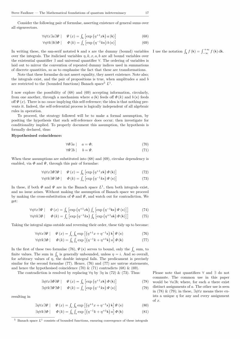
Consider the following pair of formulae, asserting existence of general sums overall eigenvectors.

∀η∀x∃a∃Ψ | Ψ (x) =∫

k

[exp

(η+1xk

)a (k)

](68)

∀η∀k∃b∃Φ | Φ (k) =∫

x

[exp

(η−1kx

)b (x)

](69)

In writing these, the san-serif notated k and x are the dummy (bound) variables I use the notation∫

k f (k) =∫ +∞−∞ f (k) dk.

over the integrals. The italicised variables η, k, x, a, b are all bound variables overthe existential quantifier ∃ and universal quantifier ∀. The ordering of variables islaid out to mirror the convention of repeated dummy indices used in summationsof discrete quantities, so as to emphasise the fact that these are transformations.

Note that these formulae do not assert equality, they assert existence. Note also;the integrals exist, and the pair of propositions is true, when amplitudes a and bare restricted to the (bounded functions) Banach space5 L1.

I now explore the possibility of (68) and (69) accepting information, circularly,from one another, through a mechanism where a (k) feeds off Φ (k) and b (x) feedsoff Ψ (x). There is no cause implying this self-reference; the idea is that nothing pre-vents it. Indeed, the self-referential process is logically independent of all algebraicrules in operation.

To proceed, the strategy followed will be to make a formal assumption, bypositing the hypothesis that such self-reference does occur; then investigate forconditionality implied. To properly document this assumption, the hypothesis isformally declared, thus:Hypothesised coincidence:

∀Φ∃a | a = Φ; (70)∀Ψ∃b | b = Ψ. (71)

When these assumptions are substituted into (68) and (69), circular dependency isenabled, via Φ and Ψ , through this pair of formulae:

∀η∀x∃Φ∃Ψ | Ψ (x) =∫

k

[exp

(η+1xk

)Φ (k)

](72)

∀η∀k∃Ψ∃Φ | Φ (k) =∫

x

[exp

(η−1kx

)Ψ (x)

](73)

In these, if both Φ and Ψ are in the Banach space L1, then both integrals exist,and no issue arises. Without making the assumption of Banach space we proceedby making the cross-substitution of Φ and Ψ , and watch out for contradiction. Weget:

∀η∀x∃Ψ | Ψ (x) =∫

k

[exp

(η+1xk

) ∫x

[exp

(η−1kx

)Ψ (x)

]](74)

∀η∀k∃Φ | Φ (k) =∫

x

[exp

(η−1kx

) ∫k

[exp

(η+1xk

)Φ (k)

]](75)

Taking the integral signs outside and reversing their order, these tidy up to become:

∀η∀x∃Ψ | Ψ (x) =∫

x

∫k exp

[(η+1x+ η−1x

)k]Ψ (x) (76)

∀η∀k∃Φ | Φ (k) =∫

k

∫x exp

[(η−1k + η+1k

)x]Φ (k) (77)

In the first of these two formulae (76), Ψ (x) serves to bound, only the∫

x sum, tofinite values. The sum in

∫k is generally unbounded, unless η = i. And so overall,

for arbitrary values of η, the double integral fails. The predicament is preciselysimilar for the second formulae (77). Hence, (76) and (77) are untrue statements,and hence the hypothesised coincidence (70) & (71) contradicts (68) & (69).

The contradiction is resolved by replacing ∀η by ∃η in (72) & (73). Thus: Please note that quantifiers ∀ and ∃ do notcommute. The common use in this paperwould be ∀a∃b; where, for each a there existdistinct assignments of a. The other use is seenin (78) & (79); in these, ∃η∀x means there ex-ists a unique η for any and every assignmentof x.

∃η∀x∃Φ∃Ψ | Ψ (x) =∫

k

[exp

(η+1xk

)Φ (k)

](78)

∃η∀k∃Ψ∃Φ | Φ (k) =∫

x

[exp

(η−1kx

)Ψ (x)

](79)

resulting in

∃η∀x∃Ψ | Ψ (x) =∫

x

∫k exp

[(η+1x+ η−1x

)k]Ψ (x) (80)

∃η∀k∃Φ | Φ (k) =∫

k

∫x exp

[(η−1k + η+1k

)x]Φ (k) (81)

5 Banach space L1 consists of bounded functions, ensuring convergence of these integrals


Releasing bound variable η from its quantifier and replacing by particular value η:

∃Ψ | Ψ (x′) =∫

x

∫k exp

[(η+1x′ + η−1x

)k]Ψ (x) (82)

∃Φ | Φ (k′) =∫

k

∫x exp

[(η−1k′ + η+1k

)x]Φ (k) (83)

These integrals exist only when η = ± i. And therefore this pair of propositions istrue — with the Hypothesised coincidence guaranteed — only for η = ± i.

But, up to this point, no imaginary information exists in the system. In order tovalidate the pair of integrals, new information must be introduced. This informationmust be assumed. To properly document this assumption, the hypothesis is formallydeclared, thus:Hypothesised existence:

∃η | η2 = −1

Setting the particular number i =√− 1 and also η = i:

∀x∃Ψ | Ψ (x) =∫

x

∫k exp [+i (x− x) k]Ψ (x) (84)

∀k∃Φ | Φ (k) =∫

k

∫x exp [−i (k − k) x]Φ (k) (85)

and in conclusion, claim that this pair of formulae are true, providing they areallowed self-referential information.

It is important to say that, within Elementary Algebra, this number’s existence isvery well-known, by Mathematical Logicians, to be logically independent [6].

11 Conclusions

Treating an algebra as a system based on axioms, those axioms prove (cause)theorems. And those theorems are logically dependent information. However, incertain algebras, there are statements and information which axioms do not prove;nor do they disprove (prevent). That information is known as logically independent.It might be thought of as having ‘null logical connectivity’ with axioms.

In this paper, a logically independent mathematical mechanism is derived,matching logical independence, linked empirically to quantum randomness. Thatmechanism comprises a logically circular, self-referential set of geometric transfor-mations, which is permitted because it does not contradict, but is consistent withsystem axioms.

Quantum indeterminacy is strictly a phenomenon of mixed states. Measurementoutcomes from pure eigenstates are never random. That is well-known. In alignmentwith that, new research of Tomasz Paterek et al shows that logical independence,also, is a strict feature of mixed states – pure states being logically dependent [12,13]. And that randomness is the response to logical independence.

That logical dependence and independence is mathematical information. Thetransition from pure states to mixed is reflected in corresponding mathematicaltransition stepping from dependence to independence. Because only mixed statesinclude indeterminate randomness, the detail, inner workings of that mathematicaltransition reveals information about the inner workings of quantum indeterminacy.

To begin, the only information in the algebraic system is the axioms, along withall theorems they prove. The transition begins to get underway following an unpre-ventable coincidence of vectors, from separate vector spaces. These coincidences arenew information to the system, which permits the onset of vectorial informationbeing passed, cyclicly, around a set of transformations. The logical circularity is inboth cyclic and anticyclic senses. The new information comes with unitary condi-tionality which transforms a geometrically definite system into one of ambiguousright and left handedness. In effect the self-referent mechanism is one of ‘sponta-neous symmetry creation’ – the converse of ‘spontaneous symmetry breaking’ – asin the Higgs mechanism.

There is nothing exceptional about the coincidences; they are assumed on a dailybasis, without noticing, by mathematicians using orthogonal vector spaces. On the


face of it, these coincidences seem like quantitative information, but they are logicalinformation, and for that reason, the creation of Hilbert space from Banach spaceis a logical matter. Notice that (finite) Banach spaces are non-orthogonal and canbe constructed purely from information in Elementary Algebra. This is ordinaryschool algebra: the algebra of scalars.

Textbook quantum theory demands: Hilbert space, self-adjoint operators andunitary symmetries, as features. From the viewpoint of the transition, none of theseare required by pure eigenstates; they are required only by mixed states. A trulyfaithful, isomorphic theory would need to be non-unitary on the pure state side ofthe transition, and unitary on the mixed state side.

Whilst the mathematician might feel free to simply declare a theory unitary, bydeclaring: observable operators should be Hermitian — although such a declarationmight seem to impose a purely quantitative restriction on variables — that eigenval-ues be real, for instance — such declaration includes hidden logical structure. Thislogical structure sits at the interface between Elementary Algebra and orthogonalLinear Algebra. The juxtaposition of these two algebras, in a single environment,is inherent in quantum mathematics, placing that logical structure squarely andunavoidably in the domain of quantum theory.

Unlike (physical) energy or momentum, that self-reference is perfectly free andnot subject to any conservation law. There is no resistance to its onset. Self-referenceis a spontaneous logical option, neither caused nor prevented (implied nor denied)by any information in the mathematical environment — it is logically independentof all information in that mathematical environment.

The effect of the self-reference is to create the consequent existence of a unitarysymmetry, along with structures that follow from it: self-adjoint operators andHilbert space, et cetera – all logically independent of the system axioms. The impactof all this is that unitarity or self-adjointness, imposed – by Postulate – is redundant.This is because unitarity and self-adjointness arise freely in the mathematics; theydon’t need to be ‘given’ to it. They occur unpreventably in Elementary algebra;they don’t need to be taken from linear algebra.

The conclusion of this research is that a quantum theory that adheres strictly tothe faithful representation of (non-unitary) pure states – that switches to – thestrict and faithful representation of (unitary) mixed states, automatically invokesrepresentation of quantum indeterminacy. Those faithful representations requireisomorphisms under two distinct systems: a non-unitary algebra representing purestates, and a unitary symmetry representing mixed. Transition between these islogically self-referential. To allow this logical mechanism to operate, unitarity (andself-adjointness) must be free to switch on and off. But in standard theory, unitarity(or self-adjointness) is imposed – by Postulate – and this freedom is blocked.

The most profound conclusion, therefore, is that unitarity and self-adjointness,imposed – by Postulate – must be given up; the benefit being a quantum theorythat expresses theory and logic of quantum indeterminacy.


References

1. Alain Aspect, Jean Dalibard, and Gérard Roger, Experimental test of Bell’s inequalitiesusing time- varying analyzers, Physical Revue Letters 49 (1982), no. 25, 1804–1807.

2. Alain Aspect, Philippe Grangier, and Gérard Roger, Experimental realization ofEinstein-Podolsky-Rosen-Bohm gedankenexperiment: A new violation of Bell’s inequal-ities, Physical Review Letters 49 (1982), no. 2, 91–94.

3. W E Baylis, J Hushilt, and Jiansu Wei, Why i?, American Journal of Physics 60 (1992),no. 9, 788–797.

4. John Bell, On the Einstein Podolsky Rosen paradox, Physics 1 (1964), 195–200.5. Gregory J Chaitin, Gödel’s theorem and information, International Journal of Physics

21 (1982), 941–954.6. Steve Faulkner, Logical independence of imaginary and complex numbers in el-

ementary algebra. [context: Theory of indeterminacy and quantum randomness],http://vixra.org/abs/1512.0286 (2015).

7. , Quantum system symmetry is not the source of unitary information in wavemechanics – context quantum randomness, http://vixra.org/abs/1510.0034 (2015).

8. , A short note on why the imaginary unit is inherent in physics,http://vixra.org/abs/1512.0452 (2015), 2.

9. D Hestenes, Vectors, spinors, and complex numbers in classical and quantum physics,American Journal of Physics 39 (1971), no. 9, 1013–1027.

10. S Kochen and E P Specker, The problem of hidden variables in quantum mechanics,Journal of Mathematics and Mechanics 17 (1967), 59–87.

11. Tomasz Paterek, Johannes Kofler, Robert Prevedel, Peter Klimek, Markus Aspelmeyer,Anton Zeilinger, and Caslav Brukner, Mathematical undecidability and quantum ran-domness, http://arxiv.org/abs/0811.4542v1 (2008), 9.

12. , Logical independence and quantum randomness, New Journal of Physics 12(2010), no. 013019, 1367–2630.

13. , Logical independence and quantum randomness — with experimental data,arxiv.org/pdf/0811.4542v2.pdf (2010).

14. Elemér E Rosinger and Gusti van Zyl, Self-referential definition of orthogonality,arXiv:90904.0082v2 (2009).

15. Edward Russell Stabler, An introduction to mathematical thought, Addison-Wesley Pub-lishing Company Inc., Reading Massachusetts USA, 1948.

16. Gergely Székely, The existence of superluminal particles is consistent with the kinematicsof Einstein’s special theory of relativity, arXiv:1202.5790v1 [physics.gen-ph] (2012).

the mathematical foundations of quantum …the mathematical foundations of quantum indeterminacy...

Documents