the matrix cookbook - university of waterloo

The Matrix Cookbook[ http://matrixcookbook.com ]

Kaare Brandt PetersenMichael Syskind Pedersen

Version: November 15, 2012

1

Introduction

What is this? These pages are a collection of facts (identities, approxima-tions, inequalities, relations, ...) about matrices and matters relating to them.It is collected in this form for the convenience of anyone who wants a quickdesktop reference .

Disclaimer: The identities, approximations and relations presented here wereobviously not invented but collected, borrowed and copied from a large amountof sources. These sources include similar but shorter notes found on the internetand appendices in books - see the references for a full list.

Errors: Very likely there are errors, typos, and mistakes for which we apolo-gize and would be grateful to receive corrections at [email protected].

Its ongoing: The project of keeping a large repository of relations involvingmatrices is naturally ongoing and the version will be apparent from the date inthe header.

Suggestions: Your suggestion for additional content or elaboration of sometopics is most welcome [email protected].

Keywords: Matrix algebra, matrix relations, matrix identities, derivative ofdeterminant, derivative of inverse matrix, di↵erentiate a matrix.

Acknowledgements: We would like to thank the following for contributionsand suggestions: Bill Baxter, Brian Templeton, Christian Rishøj, ChristianSchroppel, Dan Boley, Douglas L. Theobald, Esben Hoegh-Rasmussen, EvripidisKarseras, Georg Martius, Glynne Casteel, Jan Larsen, Jun Bin Gao, JurgenStruckmeier, Kamil Dedecius, Karim T. Abou-Moustafa, Korbinian Strimmer,Lars Christiansen, Lars Kai Hansen, Leland Wilkinson, Liguo He, Loic Thibaut,Markus Froeb, Michael Hubatka, Miguel Barao, Ole Winther, Pavel Sakov,Stephan Hattinger, Troels Pedersen, Vasile Sima, Vincent Rabaud, ZhaoshuiHe. We would also like thank The Oticon Foundation for funding our PhDstudies.

Petersen & Pedersen, The Matrix Cookbook, Version: November 15, 2012,

CONTENTS CONTENTS

Contents

1 Basics 61.1 Trace . . . . . . . . . . . . . . . . . . . . . . . . . . . . . . . . . . 61.2 Determinant . . . . . . . . . . . . . . . . . . . . . . . . . . . . . . 61.3 The Special Case 2x2 . . . . . . . . . . . . . . . . . . . . . . . . . 7

2 Derivatives 82.1 Derivatives of a Determinant . . . . . . . . . . . . . . . . . . . . 82.2 Derivatives of an Inverse . . . . . . . . . . . . . . . . . . . . . . . 92.3 Derivatives of Eigenvalues . . . . . . . . . . . . . . . . . . . . . . 102.4 Derivatives of Matrices, Vectors and Scalar Forms . . . . . . . . 102.5 Derivatives of Traces . . . . . . . . . . . . . . . . . . . . . . . . . 122.6 Derivatives of vector norms . . . . . . . . . . . . . . . . . . . . . 142.7 Derivatives of matrix norms . . . . . . . . . . . . . . . . . . . . . 142.8 Derivatives of Structured Matrices . . . . . . . . . . . . . . . . . 14

3 Inverses 173.1 Basic . . . . . . . . . . . . . . . . . . . . . . . . . . . . . . . . . . 173.2 Exact Relations . . . . . . . . . . . . . . . . . . . . . . . . . . . . 183.3 Implication on Inverses . . . . . . . . . . . . . . . . . . . . . . . . 203.4 Approximations . . . . . . . . . . . . . . . . . . . . . . . . . . . . 203.5 Generalized Inverse . . . . . . . . . . . . . . . . . . . . . . . . . . 213.6 Pseudo Inverse . . . . . . . . . . . . . . . . . . . . . . . . . . . . 21

4 Complex Matrices 244.1 Complex Derivatives . . . . . . . . . . . . . . . . . . . . . . . . . 244.2 Higher order and non-linear derivatives . . . . . . . . . . . . . . . 264.3 Inverse of complex sum . . . . . . . . . . . . . . . . . . . . . . . 27

5 Solutions and Decompositions 285.1 Solutions to linear equations . . . . . . . . . . . . . . . . . . . . . 285.2 Eigenvalues and Eigenvectors . . . . . . . . . . . . . . . . . . . . 305.3 Singular Value Decomposition . . . . . . . . . . . . . . . . . . . . 315.4 Triangular Decomposition . . . . . . . . . . . . . . . . . . . . . . 325.5 LU decomposition . . . . . . . . . . . . . . . . . . . . . . . . . . 325.6 LDM decomposition . . . . . . . . . . . . . . . . . . . . . . . . . 335.7 LDL decompositions . . . . . . . . . . . . . . . . . . . . . . . . . 33

6 Statistics and Probability 346.1 Definition of Moments . . . . . . . . . . . . . . . . . . . . . . . . 346.2 Expectation of Linear Combinations . . . . . . . . . . . . . . . . 356.3 Weighted Scalar Variable . . . . . . . . . . . . . . . . . . . . . . 36

7 Multivariate Distributions 377.1 Cauchy . . . . . . . . . . . . . . . . . . . . . . . . . . . . . . . . 377.2 Dirichlet . . . . . . . . . . . . . . . . . . . . . . . . . . . . . . . . 377.3 Normal . . . . . . . . . . . . . . . . . . . . . . . . . . . . . . . . 377.4 Normal-Inverse Gamma . . . . . . . . . . . . . . . . . . . . . . . 377.5 Gaussian . . . . . . . . . . . . . . . . . . . . . . . . . . . . . . . . 377.6 Multinomial . . . . . . . . . . . . . . . . . . . . . . . . . . . . . . 37


CONTENTS CONTENTS

7.7 Student’s t . . . . . . . . . . . . . . . . . . . . . . . . . . . . . . 377.8 Wishart . . . . . . . . . . . . . . . . . . . . . . . . . . . . . . . . 387.9 Wishart, Inverse . . . . . . . . . . . . . . . . . . . . . . . . . . . 39

8 Gaussians 408.1 Basics . . . . . . . . . . . . . . . . . . . . . . . . . . . . . . . . . 408.2 Moments . . . . . . . . . . . . . . . . . . . . . . . . . . . . . . . 428.3 Miscellaneous . . . . . . . . . . . . . . . . . . . . . . . . . . . . . 448.4 Mixture of Gaussians . . . . . . . . . . . . . . . . . . . . . . . . . 44

9 Special Matrices 469.1 Block matrices . . . . . . . . . . . . . . . . . . . . . . . . . . . . 469.2 Discrete Fourier Transform Matrix, The . . . . . . . . . . . . . . 479.3 Hermitian Matrices and skew-Hermitian . . . . . . . . . . . . . . 489.4 Idempotent Matrices . . . . . . . . . . . . . . . . . . . . . . . . . 499.5 Orthogonal matrices . . . . . . . . . . . . . . . . . . . . . . . . . 499.6 Positive Definite and Semi-definite Matrices . . . . . . . . . . . . 509.7 Singleentry Matrix, The . . . . . . . . . . . . . . . . . . . . . . . 529.8 Symmetric, Skew-symmetric/Antisymmetric . . . . . . . . . . . . 549.9 Toeplitz Matrices . . . . . . . . . . . . . . . . . . . . . . . . . . . 549.10 Transition matrices . . . . . . . . . . . . . . . . . . . . . . . . . . 559.11 Units, Permutation and Shift . . . . . . . . . . . . . . . . . . . . 569.12 Vandermonde Matrices . . . . . . . . . . . . . . . . . . . . . . . . 57

10 Functions and Operators 5810.1 Functions and Series . . . . . . . . . . . . . . . . . . . . . . . . . 5810.2 Kronecker and Vec Operator . . . . . . . . . . . . . . . . . . . . 5910.3 Vector Norms . . . . . . . . . . . . . . . . . . . . . . . . . . . . . 6110.4 Matrix Norms . . . . . . . . . . . . . . . . . . . . . . . . . . . . . 6110.5 Rank . . . . . . . . . . . . . . . . . . . . . . . . . . . . . . . . . . 6210.6 Integral Involving Dirac Delta Functions . . . . . . . . . . . . . . 6210.7 Miscellaneous . . . . . . . . . . . . . . . . . . . . . . . . . . . . . 63

A One-dimensional Results 64A.1 Gaussian . . . . . . . . . . . . . . . . . . . . . . . . . . . . . . . . 64A.2 One Dimensional Mixture of Gaussians . . . . . . . . . . . . . . . 65

B Proofs and Details 66B.1 Misc Proofs . . . . . . . . . . . . . . . . . . . . . . . . . . . . . . 66


CONTENTS CONTENTS

Notation and Nomenclature

A MatrixAij Matrix indexed for some purposeAi Matrix indexed for some purposeAij Matrix indexed for some purposeAn Matrix indexed for some purpose or

The n.th power of a square matrixA�1 The inverse matrix of the matrix AA+ The pseudo inverse matrix of the matrix A (see Sec. 3.6)A1/2 The square root of a matrix (if unique), not elementwise(A)ij The (i, j).th entry of the matrix AAij The (i, j).th entry of the matrix A[A]ij The ij-submatrix, i.e. A with i.th row and j.th column deleteda Vector (column-vector)ai Vector indexed for some purposeai The i.th element of the vector aa Scalar

<z Real part of a scalar<z Real part of a vector<Z Real part of a matrix=z Imaginary part of a scalar=z Imaginary part of a vector=Z Imaginary part of a matrix

det(A) Determinant of ATr(A) Trace of the matrix Adiag(A) Diagonal matrix of the matrix A, i.e. (diag(A))ij = �ijAij

eig(A) Eigenvalues of the matrix Avec(A) The vector-version of the matrix A (see Sec. 10.2.2)sup Supremum of a set||A|| Matrix norm (subscript if any denotes what norm)AT Transposed matrixA�T The inverse of the transposed and vice versa, A�T = (A�1)T = (AT )�1.A⇤ Complex conjugated matrixAH Transposed and complex conjugated matrix (Hermitian)

A �B Hadamard (elementwise) productA⌦B Kronecker product

0 The null matrix. Zero in all entries.I The identity matrixJij The single-entry matrix, 1 at (i, j) and zero elsewhere⌃ A positive definite matrix⇤ A diagonal matrix


1 BASICS

1 Basics

(AB)�1 = B�1A�1 (1)

(ABC...)�1 = ...C�1B�1A�1 (2)

(AT )�1 = (A�1)T (3)

(A+B)T = AT +BT (4)

(AB)T = BTAT (5)

(ABC...)T = ...CTBTAT (6)

(AH)�1 = (A�1)H (7)

(A+B)H = AH +BH (8)

(AB)H = BHAH (9)

(ABC...)H = ...CHBHAH (10)

1.1 Trace

Tr(A) =P

iAii (11)

Tr(A) =P

i�i, �i = eig(A) (12)

Tr(A) = Tr(AT ) (13)

Tr(AB) = Tr(BA) (14)

Tr(A+B) = Tr(A) + Tr(B) (15)

Tr(ABC) = Tr(BCA) = Tr(CAB) (16)

aTa = Tr(aaT ) (17)

1.2 Determinant

Let A be an n⇥ n matrix.

det(A) =Q

i�i �i = eig(A) (18)

det(cA) = cn det(A), if A 2 Rn⇥n (19)

det(AT ) = det(A) (20)

det(AB) = det(A) det(B) (21)

det(A�1) = 1/ det(A) (22)

det(An) = det(A)n (23)

det(I+ uvT ) = 1 + uTv (24)

For n = 2:det(I+A) = 1 + det(A) + Tr(A) (25)

For n = 3:

det(I+A) = 1 + det(A) + Tr(A) +1

2Tr(A)2 � 1

2Tr(A2) (26)


1.3 The Special Case 2x2 1 BASICS

For n = 4:

det(I+A) = 1 + det(A) + Tr(A) +1

2

+Tr(A)2 � 1

2Tr(A2)

+1

6Tr(A)3 � 1

2Tr(A)Tr(A2) +

1

3Tr(A3) (27)

For small ", the following approximation holds

det(I+ "A) ⇠= 1 + det(A) + "Tr(A) +1

2"2Tr(A)2 � 1

2"2Tr(A2) (28)

1.3 The Special Case 2x2

Consider the matrix A

A =

A

11

A12

A21

A22

�

Determinant and trace

det(A) = A11

A22

�A12

A21

(29)

Tr(A) = A11

+A22

(30)

Eigenvalues�2 � � · Tr(A) + det(A) = 0

�1

=Tr(A) +

pTr(A)2 � 4 det(A)

2�2

=Tr(A)�pTr(A)2 � 4 det(A)

2

�1

+ �2

= Tr(A) �1

�2

= det(A)

Eigenvectors

v1

/

A12

�1

�A11

�v2

/

A12

�2

�A11

�

Inverse

A�1 =1

det(A)

A

22

�A12

�A21

A11

�(31)


2 DERIVATIVES

2 Derivatives

This section is covering di↵erentiation of a number of expressions with respect toa matrix X. Note that it is always assumed that X has no special structure, i.e.that the elements of X are independent (e.g. not symmetric, Toeplitz, positivedefinite). See section 2.8 for di↵erentiation of structured matrices. The basicassumptions can be written in a formula as

@Xkl

@Xij= �ik�lj (32)

that is for e.g. vector forms,

@x

@y

�

i

=@xi

@y

@x

@y

�

i

=@x

@yi

@x

@y

�

ij

=@xi

@yj

The following rules are general and very useful when deriving the di↵erential ofan expression ([19]):

@A = 0 (A is a constant) (33)@(↵X) = ↵@X (34)

@(X+Y) = @X+ @Y (35)@(Tr(X)) = Tr(@X) (36)@(XY) = (@X)Y+X(@Y) (37)

@(X �Y) = (@X) �Y+X � (@Y) (38)@(X⌦Y) = (@X)⌦Y+X⌦ (@Y) (39)

@(X�1) = �X�1(@X)X�1 (40)@(det(X)) = Tr(adj(X)@X) (41)@(det(X)) = det(X)Tr(X�1@X) (42)

@(ln(det(X))) = Tr(X�1@X) (43)@XT = (@X)T (44)@XH = (@X)H (45)

2.1 Derivatives of a Determinant

2.1.1 General form

@ det(Y)

@x= det(Y)Tr

Y�1

@Y

@x

�(46)

X

k

@ det(X)

@XikXjk = �ij det(X) (47)

@2 det(Y)

@x2

= det(Y)

"Tr

"Y�1

@ @Y@x

@x

#

+Tr

Y�1

@Y

@x

�Tr

Y�1

@Y

@x

�

�Tr

✓Y�1

@Y

@x

◆✓Y�1

@Y

@x

◆�#(48)


2.2 Derivatives of an Inverse 2 DERIVATIVES

2.1.2 Linear forms

@ det(X)

@X= det(X)(X�1)T (49)

X

k

@ det(X)

@XikXjk = �ij det(X) (50)

@ det(AXB)

@X= det(AXB)(X�1)T = det(AXB)(XT )�1 (51)

2.1.3 Square forms

If X is square and invertible, then

@ det(XTAX)

@X= 2det(XTAX)X�T (52)

If X is not square but A is symmetric, then

@ det(XTAX)

@X= 2det(XTAX)AX(XTAX)�1 (53)

If X is not square and A is not symmetric, then

@ det(XTAX)

@X= det(XTAX)(AX(XTAX)�1 +ATX(XTATX)�1) (54)

2.1.4 Other nonlinear forms

Some special cases are (See [9, 7])

@ ln det(XTX)|@X

= 2(X+)T (55)

@ ln det(XTX)

@X+

= �2XT (56)

@ ln | det(X)|@X

= (X�1)T = (XT )�1 (57)

@ det(Xk)

@X= k det(Xk)X�T (58)

2.2 Derivatives of an Inverse

From [27] we have the basic identity

@Y�1

@x= �Y�1

@Y

@xY�1 (59)


2.3 Derivatives of Eigenvalues 2 DERIVATIVES

from which it follows

@(X�1)kl@Xij

= �(X�1)ki(X�1)jl (60)

@aTX�1b

@X= �X�TabTX�T (61)

@ det(X�1)

@X= � det(X�1)(X�1)T (62)

@Tr(AX�1B)

@X= �(X�1BAX�1)T (63)

@Tr((X+A)�1)

@X= �((X+A)�1(X+A)�1)T (64)

From [32] we have the following result: Let A be an n⇥ n invertible squarematrix, W be the inverse of A, and J(A) is an n⇥n -variate and di↵erentiablefunction with respect to A, then the partial di↵erentials of J with respect to Aand W satisfy

@J

@A= �A�T @J

@WA�T

2.3 Derivatives of Eigenvalues

@

@X

Xeig(X) =

@

@XTr(X) = I (65)

@

@X

Yeig(X) =

@

@Xdet(X) = det(X)X�T (66)

If A is real and symmetric, �i and vi are distinct eigenvalues and eigenvectorsof A (see (276)) with vT

i vi = 1, then [33]

@�i = vTi @(A)vi (67)

@vi = (�iI�A)+@(A)vi (68)

2.4 Derivatives of Matrices, Vectors and Scalar Forms

2.4.1 First Order

@xTa

@x=

@aTx

@x= a (69)

@aTXb

@X= abT (70)

@aTXTb

@X= baT (71)

@aTXa

@X=

@aTXTa

@X= aaT (72)

@X

@Xij= Jij (73)

@(XA)ij@Xmn

= �im(A)nj = (JmnA)ij (74)

@(XTA)ij@Xmn

= �in(A)mj = (JnmA)ij (75)


2.4 Derivatives of Matrices, Vectors and Scalar Forms 2 DERIVATIVES

2.4.2 Second Order

@

@Xij

X

klmn

XklXmn = 2X

kl

Xkl (76)

@bTXTXc

@X= X(bcT + cbT ) (77)

@(Bx+ b)TC(Dx+ d)

@x= BTC(Dx+ d) +DTCT (Bx+ b) (78)

@(XTBX)kl@Xij

= �lj(XTB)ki + �kj(BX)il (79)

@(XTBX)

@Xij= XTBJij + JjiBX (Jij)kl = �ik�jl (80)

See Sec 9.7 for useful properties of the Single-entry matrix Jij

@xTBx

@x= (B+BT )x (81)

@bTXTDXc

@X= DTXbcT +DXcbT (82)

@

@X(Xb+ c)TD(Xb+ c) = (D+DT )(Xb+ c)bT (83)

Assume W is symmetric, then

@

@s(x�As)TW(x�As) = �2ATW(x�As) (84)

@

@x(x� s)TW(x� s) = 2W(x� s) (85)

@

@s(x� s)TW(x� s) = �2W(x� s) (86)

@

@x(x�As)TW(x�As) = 2W(x�As) (87)

@

@A(x�As)TW(x�As) = �2W(x�As)sT (88)

As a case with complex values the following holds

@(a� xHb)2

@x= �2b(a� xHb)⇤ (89)

This formula is also known from the LMS algorithm [14]

2.4.3 Higher-order and non-linear

@(Xn)kl@Xij

=n�1X

r=0

(XrJijXn�1�r)kl (90)

For proof of the above, see B.1.3.

@

@XaTXnb =

n�1X

r=0

(Xr)TabT (Xn�1�r)T (91)


2.5 Derivatives of Traces 2 DERIVATIVES

@

@XaT (Xn)TXnb =

n�1X

r=0

hXn�1�rabT (Xn)TXr

+(Xr)TXnabT (Xn�1�r)Ti

(92)

See B.1.3 for a proof.Assume s and r are functions of x, i.e. s = s(x), r = r(x), and that A is aconstant, then

@

@xsTAr =

@s

@x

�TAr+

@r

@x

�TAT s (93)

@

@x

(Ax)T (Ax)

(Bx)T (Bx)=

@

@x

xTATAx

xTBTBx(94)

= 2ATAx

xTBBx� 2

xTATAxBTBx

(xTBTBx)2(95)

2.4.4 Gradient and Hessian

Using the above we have for the gradient and the Hessian

f = xTAx+ bTx (96)

rx

f =@f

@x= (A+AT )x+ b (97)

@2f

@x@xT= A+AT (98)

2.5 Derivatives of Traces

Assume F (X) to be a di↵erentiable function of each of the elements of X. Itthen holds that

@Tr(F (X))

@X= f(X)T

where f(·) is the scalar derivative of F (·).

2.5.1 First Order

@

@XTr(X) = I (99)

@

@XTr(XA) = AT (100)

@

@XTr(AXB) = ATBT (101)

@

@XTr(AXTB) = BA (102)

@

@XTr(XTA) = A (103)

@

@XTr(AXT ) = A (104)

@

@XTr(A⌦X) = Tr(A)I (105)


2.5 Derivatives of Traces 2 DERIVATIVES

2.5.2 Second Order

@

@XTr(X2) = 2XT (106)

@

@XTr(X2B) = (XB+BX)T (107)

@

@XTr(XTBX) = BX+BTX (108)

@

@XTr(BXXT ) = BX+BTX (109)

@

@XTr(XXTB) = BX+BTX (110)

@

@XTr(XBXT ) = XBT +XB (111)

@

@XTr(BXTX) = XBT +XB (112)

@

@XTr(XTXB) = XBT +XB (113)

@

@XTr(AXBX) = ATXTBT +BTXTAT (114)

@

@XTr(XTX) =

@

@XTr(XXT ) = 2X (115)

@

@XTr(BTXTCXB) = CTXBBT +CXBBT (116)

@

@XTr⇥XTBXC

⇤= BXC+BTXCT (117)

@

@XTr(AXBXTC) = ATCTXBT +CAXB (118)

@

@XTrh(AXB+C)(AXB+C)T

i= 2AT (AXB+C)BT (119)

@

@XTr(X⌦X) =

@

@XTr(X)Tr(X) = 2Tr(X)I(120)

See [7].

2.5.3 Higher Order

@

@XTr(Xk) = k(Xk�1)T (121)

@

@XTr(AXk) =

k�1X

r=0

(XrAXk�r�1)T (122)

@@XTr

⇥BTXTCXXTCXB

⇤= CXXTCXBBT

+CTXBBTXTCTX

+CXBBTXTCX

+CTXXTCTXBBT (123)


2.6 Derivatives of vector norms 2 DERIVATIVES

2.5.4 Other

@

@XTr(AX�1B) = �(X�1BAX�1)T = �X�TATBTX�T (124)

Assume B and C to be symmetric, then

@

@XTrh(XTCX)�1A

i= �(CX(XTCX)�1)(A+AT )(XTCX)�1 (125)

@

@XTrh(XTCX)�1(XTBX)

i= �2CX(XTCX)�1XTBX(XTCX)�1

+2BX(XTCX)�1 (126)

@

@XTrh(A+XTCX)�1(XTBX)

i= �2CX(A+XTCX)�1XTBX(A+XTCX)�1

+2BX(A+XTCX)�1 (127)

See [7].

@Tr(sin(X))

@X= cos(X)T (128)

2.6 Derivatives of vector norms

2.6.1 Two-norm

@

@x||x� a||

2

=x� a

||x� a||2

(129)

@

@x

x� a

kx� ak2

=I

kx� ak2

� (x� a)(x� a)T

kx� ak32

(130)

@||x||22

@x=

@||xTx||2

@x= 2x (131)

2.7 Derivatives of matrix norms

For more on matrix norms, see Sec. 10.4.

2.7.1 Frobenius norm

@

@X||X||2

F

=@

@XTr(XXH) = 2X (132)

See (248). Note that this is also a special case of the result in equation 119.

2.8 Derivatives of Structured Matrices

Assume that the matrix A has some structure, i.e. symmetric, toeplitz, etc.In that case the derivatives of the previous section does not apply in general.Instead, consider the following general rule for di↵erentiating a scalar functionf(A)

df

dAij=X

kl

@f

@Akl

@Akl

@Aij= Tr

"@f

@A

�T@A

@Aij

#(133)


2.8 Derivatives of Structured Matrices 2 DERIVATIVES

The matrix di↵erentiated with respect to itself is in this document referred toas the structure matrix of A and is defined simply by

@A

@Aij= Sij (134)

If A has no special structure we have simply Sij = Jij , that is, the structurematrix is simply the single-entry matrix. Many structures have a representationin singleentry matrices, see Sec. 9.7.6 for more examples of structure matrices.

2.8.1 The Chain Rule

Sometimes the objective is to find the derivative of a matrix which is a functionof another matrix. Let U = f(X), the goal is to find the derivative of thefunction g(U) with respect to X:

@g(U)

@X=

@g(f(X))

@X(135)

Then the Chain Rule can then be written the following way:

@g(U)

@X=

@g(U)

@xij=

MX

k=1

NX

l=1

@g(U)

@ukl

@ukl

@xij(136)

Using matrix notation, this can be written as:

@g(U)

@Xij= Tr

h(@g(U)

@U)T

@U

@Xij

i. (137)

2.8.2 Symmetric

If A is symmetric, then Sij = Jij + Jji � JijJij and therefore

df

dA=

@f

@A

�+

@f

@A

�T� diag

@f

@A

�(138)

That is, e.g., ([5]):

@Tr(AX)

@X= A+AT � (A � I), see (142) (139)

@ det(X)

@X= det(X)(2X�1 � (X�1 � I)) (140)

@ ln det(X)

@X= 2X�1 � (X�1 � I) (141)

2.8.3 Diagonal

If X is diagonal, then ([19]):

@Tr(AX)

@X= A � I (142)


2.8 Derivatives of Structured Matrices 2 DERIVATIVES

2.8.4 Toeplitz

Like symmetric matrices and diagonal matrices also Toeplitz matrices has aspecial structure which should be taken into account when the derivative withrespect to a matrix with Toeplitz structure.

@Tr(AT)

@T(143)

=@Tr(TA)

@T

=

2

666664

Tr(A) Tr([AT ]n1) Tr([[AT ]1n]n�1,2) · · · An1

Tr([AT ]1n)) Tr(A)

...

...

.

.

.

Tr([[AT ]1n]2,n�1)

...

...

... Tr([[AT ]1n]n�1,2)

.

.

.

...

...

... Tr([AT ]n1)

A1n · · · Tr([[AT ]1n]2,n�1) Tr([AT ]1n)) Tr(A)

3

777775

⌘ ↵(A)

As it can be seen, the derivative ↵(A) also has a Toeplitz structure. Each valuein the diagonal is the sum of all the diagonal valued in A, the values in thediagonals next to the main diagonal equal the sum of the diagonal next to themain diagonal in AT . This result is only valid for the unconstrained Toeplitzmatrix. If the Toeplitz matrix also is symmetric, the same derivative yields

@Tr(AT)

@T=

@Tr(TA)

@T= ↵(A) +↵(A)T �↵(A) � I (144)


3 INVERSES

3 Inverses

3.1 Basic

3.1.1 Definition

The inverse A�1 of a matrix A 2 Cn⇥n is defined such that

AA�1 = A�1A = I, (145)

where I is the n⇥n identity matrix. If A�1 exists, A is said to be nonsingular.Otherwise, A is said to be singular (see e.g. [12]).

3.1.2 Cofactors and Adjoint

The submatrix of a matrix A, denoted by [A]ij is a (n � 1) ⇥ (n � 1) matrixobtained by deleting the ith row and the jth column of A. The (i, j) cofactorof a matrix is defined as

cof(A, i, j) = (�1)i+j det([A]ij), (146)

The matrix of cofactors can be created from the cofactors

cof(A) =

2

666664

cof(A, 1, 1) · · · cof(A, 1, n)

... cof(A, i, j)...

cof(A, n, 1) · · · cof(A, n, n)

3

777775(147)

The adjoint matrix is the transpose of the cofactor matrix

adj(A) = (cof(A))T , (148)

3.1.3 Determinant

The determinant of a matrix A 2 Cn⇥n is defined as (see [12])

det(A) =nX

j=1

(�1)j+1A1j det ([A]

1j) (149)

=nX

j=1

A1jcof(A, 1, j). (150)

3.1.4 Construction

The inverse matrix can be constructed, using the adjoint matrix, by

A�1 =1

det(A)· adj(A) (151)

For the case of 2⇥ 2 matrices, see section 1.3.


3.2 Exact Relations 3 INVERSES

3.1.5 Condition number

The condition number of a matrix c(A) is the ratio between the largest and thesmallest singular value of a matrix (see Section 5.3 on singular values),

c(A) =d+

d�(152)

The condition number can be used to measure how singular a matrix is. If thecondition number is large, it indicates that the matrix is nearly singular. Thecondition number can also be estimated from the matrix norms. Here

c(A) = kAk · kA�1k, (153)

where k · k is a norm such as e.g the 1-norm, the 2-norm, the 1-norm or theFrobenius norm (see Sec 10.4 for more on matrix norms).

The 2-norm of A equalsp

(max(eig(AHA))) [12, p.57]. For a symmetricmatrix, this reduces to ||A||

2

= max(|eig(A)|) [12, p.394]. If the matrix issymmetric and positive definite, ||A||

2

= max(eig(A)). The condition numberbased on the 2-norm thus reduces to

kAk2

kA�1k2

= max(eig(A))max(eig(A�1)) =max(eig(A))

min(eig(A)). (154)

3.2 Exact Relations

3.2.1 Basic

(AB)�1 = B�1A�1 (155)

3.2.2 The Woodbury identity

The Woodbury identity comes in many variants. The latter of the two can befound in [12]

(A+CBCT )�1 = A�1 �A�1C(B�1 +CTA�1C)�1CTA�1 (156)

(A+UBV)�1 = A�1 �A�1U(B�1 +VA�1U)�1VA�1 (157)

If P,R are positive definite, then (see [30])

(P�1 +BTR�1B)�1BTR�1 = PBT (BPBT +R)�1 (158)

3.2.3 The Kailath Variant

(A+BC)�1 = A�1 �A�1B(I+CA�1B)�1CA�1 (159)

See [4, page 153].

3.2.4 Sherman-Morrison

(A+ bcT )�1 = A�1 � A�1bcTA�1

1 + cTA�1b(160)


3.2 Exact Relations 3 INVERSES

3.2.5 The Searle Set of Identities

The following set of identities, can be found in [25, page 151],

(I+A�1)�1 = A(A+ I)�1 (161)

(A+BBT )�1B = A�1B(I+BTA�1B)�1 (162)

(A�1 +B�1)�1 = A(A+B)�1B = B(A+B)�1A (163)

A�A(A+B)�1A = B�B(A+B)�1B (164)

A�1 +B�1 = A�1(A+B)B�1 (165)

(I+AB)�1 = I�A(I+BA)�1B (166)

(I+AB)�1A = A(I+BA)�1 (167)

3.2.6 Rank-1 update of inverse of inner product

Denote A = (XTX)�1 and that X is extended to include a new column vectorin the end X = [X v]. Then [34]

(XT X)�1 =

"A+ AX

Tvv

TXA

T

v

Tv�v

TXAX

Tv

�AX

Tv

v

Tv�v

TXAX

Tv

�v

TXA

T

v

Tv�v

TXAX

Tv

1

v

Tv�v

TXAX

Tv

#

3.2.7 Rank-1 update of Moore-Penrose Inverse

The following is a rank-1 update for the Moore-Penrose pseudo-inverse of realvalued matrices and proof can be found in [18]. The matrix G is defined below:

(A+ cdT )+ = A+ +G (168)

Using the the notation

� = 1 + dTA+c (169)

v = A+c (170)

n = (A+)Td (171)

w = (I�AA+)c (172)

m = (I�A+A)Td (173)

the solution is given as six di↵erent cases, depending on the entities ||w||,||m||, and �. Please note, that for any (column) vector v it holds that v+ =

vT (vTv)�1 = v

T

||v||2 . The solution is:

Case 1 of 6: If ||w|| 6= 0 and ||m|| 6= 0. Then

G = �vw+ � (m+)TnT + �(m+)Tw+ (174)

= � 1

||w||2vwT � 1

||m||2mnT +�

||m||2||w||2mwT (175)

Case 2 of 6: If ||w|| = 0 and ||m|| 6= 0 and � = 0. Then

G = �vv+A+ � (m+)TnT (176)

= � 1

||v||2vvTA+ � 1

||m||2mnT (177)


3.3 Implication on Inverses 3 INVERSES

Case 3 of 6: If ||w|| = 0 and � 6= 0. Then

G =1

�mvTA+ � �

||v||2||m||2 + |�|2✓ ||v||2

�m+ v

◆✓ ||m||2�

(A+)Tv + n

◆T

(178)Case 4 of 6: If ||w|| 6= 0 and ||m|| = 0 and � = 0. Then

G = �A+nn+ � vw+ (179)

= � 1

||n||2A+nnT � 1

||w||2vwT (180)

Case 5 of 6: If ||m|| = 0 and � 6= 0. Then

G =1

�A+nwT � �

||n||2||w||2 + |�|2✓ ||w||2

�A+n+ v

◆✓ ||n||2�

w + n

◆T

(181)

Case 6 of 6: If ||w|| = 0 and ||m|| = 0 and � = 0. Then

G = �vv+A+ �A+nn+ + v+A+nvn+ (182)

= � 1

||v||2vvTA+ � 1

||n||2A+nnT +

vTA+n

||v||2||n||2vnT (183)

3.3 Implication on Inverses

If (A+B)�1 = A�1 +B�1 then AB�1A = BA�1B (184)

See [25].

3.3.1 A PosDef identity

Assume P,R to be positive definite and invertible, then

(P�1 +BTR�1B)�1BTR�1 = PBT (BPBT +R)�1 (185)

See [30].

3.4 Approximations

The following identity is known as the Neuman series of a matrix, which holdswhen |�i| < 1 for all eigenvalues �i

(I�A)�1 =1X

n=0

An (186)

which is equivalent to

(I+A)�1 =1X

n=0

(�1)nAn (187)

When |�i| < 1 for all eigenvalues �i, it holds that A ! 0 for n ! 1, and thefollowing approximations holds

(I�A)�1 ⇠= I+A+A2 (188)

(I+A)�1 ⇠= I�A+A2 (189)


3.5 Generalized Inverse 3 INVERSES

The following approximation is from [22] and holds when A large and symmetric

A�A(I+A)�1A ⇠= I�A�1 (190)

If �2 is small compared to Q and M then

(Q+ �2M)�1 ⇠= Q�1 � �2Q�1MQ�1 (191)

Proof:

(Q+ �2M)�1 = (192)

(QQ�1Q+ �2MQ�1Q)�1 = (193)

((I+ �2MQ�1)Q)�1 = (194)

Q�1(I+ �2MQ�1)�1 (195)

This can be rewritten using the Taylor expansion:

Q�1(I+ �2MQ�1)�1 = (196)

Q�1(I� �2MQ�1 + (�2MQ�1)2 � ...) ⇠= Q�1 � �2Q�1MQ�1 (197)

3.5 Generalized Inverse

3.5.1 Definition

A generalized inverse matrix of the matrix A is any matrix A� such that (see[26])

AA�A = A (198)

The matrix A� is not unique.

3.6 Pseudo Inverse

3.6.1 Definition

The pseudo inverse (or Moore-Penrose inverse) of a matrix A is the matrix A+

that fulfils

I AA+A = A

II A+AA+ = A+

III AA+ symmetric

IV A+A symmetric

The matrix A+ is unique and does always exist. Note that in case of com-plex matrices, the symmetric condition is substituted by a condition of beingHermitian.


3.6 Pseudo Inverse 3 INVERSES

3.6.2 Properties

Assume A+ to be the pseudo-inverse of A, then (See [3] for some of them)

(A+)+ = A (199)

(AT )+ = (A+)T (200)

(AH)+ = (A+)H (201)

(A⇤)+ = (A+)⇤ (202)

(A+A)AH = AH (203)

(A+A)AT 6= AT (204)

(cA)+ = (1/c)A+ (205)

A+ = (ATA)+AT (206)

A+ = AT (AAT )+ (207)

(ATA)+ = A+(AT )+ (208)

(AAT )+ = (AT )+A+ (209)

A+ = (AHA)+AH (210)

A+ = AH(AAH)+ (211)

(AHA)+ = A+(AH)+ (212)

(AAH)+ = (AH)+A+ (213)

(AB)+ = (A+AB)+(ABB+)+ (214)

f(AHA)� f(0)I = A+[f(AAH)� f(0)I]A (215)

f(AAH)� f(0)I = A[f(AHA)� f(0)I]A+ (216)

where A 2 Cn⇥m.Assume A to have full rank, then

(AA+)(AA+) = AA+ (217)

(A+A)(A+A) = A+A (218)

Tr(AA+) = rank(AA+) (See [26]) (219)

Tr(A+A) = rank(A+A) (See [26]) (220)

For two matrices it hold that

(AB)+ = (A+AB)+(ABB+)+ (221)

(A⌦B)+ = A+ ⌦B+ (222)

3.6.3 Construction

Assume that A has full rank, then

A n⇥ n Square rank(A) = n ) A+ = A�1

A n⇥m Broad rank(A) = n ) A+ = AT (AAT )�1

A n⇥m Tall rank(A) = m ) A+ = (ATA)�1AT

The so-called ”broad version” is also known as right inverse and the ”tall ver-sion” as the left inverse.


3.6 Pseudo Inverse 3 INVERSES

Assume A does not have full rank, i.e. A is n ⇥ m and rank(A) = r <min(n,m). The pseudo inverse A+ can be constructed from the singular valuedecomposition A = UDVT , by

A+ = VrD�1

r UTr (223)

where Ur,Dr, and Vr are the matrices with the degenerated rows and columnsdeleted. A di↵erent way is this: There do always exist two matrices C n ⇥ rand D r ⇥m of rank r, such that A = CD. Using these matrices it holds that

A+ = DT (DDT )�1(CTC)�1CT (224)

See [3].


4 COMPLEX MATRICES

4 Complex Matrices

The complex scalar product r = pq can be written as <r

=r�=

<p �=p=p <p

� <q=q

�(225)

4.1 Complex Derivatives

In order to di↵erentiate an expression f(z) with respect to a complex z, theCauchy-Riemann equations have to be satisfied ([7]):

df(z)

dz=

@<(f(z))@<z + i

@=(f(z))@<z (226)

anddf(z)

dz= �i

@<(f(z))@=z +

@=(f(z))@=z (227)

or in a more compact form:

@f(z)

@=z = i@f(z)

@<z . (228)

A complex function that satisfies the Cauchy-Riemann equations for points in aregion R is said yo be analytic in this region R. In general, expressions involvingcomplex conjugate or conjugate transpose do not satisfy the Cauchy-Riemannequations. In order to avoid this problem, a more generalized definition ofcomplex derivative is used ([24], [6]):

• Generalized Complex Derivative:

df(z)

dz=

1

2

⇣@f(z)@<z � i

@f(z)

@=z⌘. (229)

• Conjugate Complex Derivative

df(z)

dz⇤=

1

2

⇣@f(z)@<z + i

@f(z)

@=z⌘. (230)

The Generalized Complex Derivative equals the normal derivative, when f is ananalytic function. For a non-analytic function such as f(z) = z⇤, the derivativeequals zero. The Conjugate Complex Derivative equals zero, when f is ananalytic function. The Conjugate Complex Derivative has e.g been used by [21]when deriving a complex gradient.Notice:

df(z)

dz6= @f(z)

@<z + i@f(z)

@=z . (231)

• Complex Gradient Vector: If f is a real function of a complex vector z,then the complex gradient vector is given by ([14, p. 798])

rf(z) = 2df(z)

dz⇤(232)

=@f(z)

@<z + i@f(z)

@=z .


4.1 Complex Derivatives 4 COMPLEX MATRICES

• Complex Gradient Matrix: If f is a real function of a complex matrix Z,then the complex gradient matrix is given by ([2])

rf(Z) = 2df(Z)

dZ⇤ (233)

=@f(Z)

@<Z + i@f(Z)

@=Z .

These expressions can be used for gradient descent algorithms.

4.1.1 The Chain Rule for complex numbers

The chain rule is a little more complicated when the function of a complexu = f(x) is non-analytic. For a non-analytic function, the following chain rulecan be applied ([7])

@g(u)

@x=

@g

@u

@u

@x+

@g

@u⇤@u⇤

@x(234)

=@g

@u

@u

@x+⇣@g⇤

@u

⌘⇤ @u⇤

@x

Notice, if the function is analytic, the second term reduces to zero, and the func-tion is reduced to the normal well-known chain rule. For the matrix derivativeof a scalar function g(U), the chain rule can be written the following way:

@g(U)

@X=

Tr((@g(U)

@U )T@U)

@X+

Tr((@g(U)

@U⇤ )T@U⇤)

@X. (235)

4.1.2 Complex Derivatives of Traces

If the derivatives involve complex numbers, the conjugate transpose is often in-volved. The most useful way to show complex derivative is to show the derivativewith respect to the real and the imaginary part separately. An easy example is:

@Tr(X⇤)

@<X =@Tr(XH)

@<X = I (236)

i@Tr(X⇤)

@=X = i@Tr(XH)

@=X = I (237)

Since the two results have the same sign, the conjugate complex derivative (230)should be used.

@Tr(X)

@<X =@Tr(XT )

@<X = I (238)

i@Tr(X)

@=X = i@Tr(XT )

@=X = �I (239)

Here, the two results have di↵erent signs, and the generalized complex derivative(229) should be used. Hereby, it can be seen that (100) holds even if X is acomplex number.

@Tr(AXH)

@<X = A (240)

i@Tr(AXH)

@=X = A (241)


4.2 Higher order and non-linear derivatives 4 COMPLEX MATRICES

@Tr(AX⇤)

@<X = AT (242)

i@Tr(AX⇤)

@=X = AT (243)

@Tr(XXH)

@<X =@Tr(XHX)

@<X = 2<X (244)

i@Tr(XXH)

@=X = i@Tr(XHX)

@=X = i2=X (245)

By inserting (244) and (245) in (229) and (230), it can be seen that

@Tr(XXH)

@X= X⇤ (246)

@Tr(XXH)

@X⇤ = X (247)

Since the function Tr(XXH) is a real function of the complex matrix X, thecomplex gradient matrix (233) is given by

rTr(XXH) = 2@Tr(XXH)

@X⇤ = 2X (248)

4.1.3 Complex Derivative Involving Determinants

Here, a calculation example is provided. The objective is to find the derivative ofdet(XHAX) with respect to X 2 Cm⇥n. The derivative is found with respect tothe real part and the imaginary part of X, by use of (42) and (37), det(XHAX)can be calculated as (see App. B.1.4 for details)

@ det(XHAX)

@X=

1

2

⇣@ det(XHAX)

@<X � i@ det(XHAX)

@=X⌘

= det(XHAX)�(XHAX)�1XHA

�T(249)

and the complex conjugate derivative yields

@ det(XHAX)

@X⇤ =1

2

⇣@ det(XHAX)

@<X + i@ det(XHAX)

@=X⌘

= det(XHAX)AX(XHAX)�1 (250)

4.2 Higher order and non-linear derivatives

@

@x

(Ax)H(Ax)

(Bx)H(Bx)=

@

@x

xHAHAx

xHBHBx(251)

= 2AHAx

xHBBx� 2

xHAHAxBHBx

(xHBHBx)2(252)


4.3 Inverse of complex sum 4 COMPLEX MATRICES

4.3 Inverse of complex sum

Given real matrices A,B find the inverse of the complex sum A + iB. Formthe auxiliary matrices

E = A+ tB (253)

F = B� tA, (254)

and find a value of t such that E�1 exists. Then

(A+ iB)�1 = (1� it)(E+ iF)�1 (255)

= (1� it)((E+ FE�1F)�1 � i(E+ FE�1F)�1FE�1)(256)

= (1� it)(E+ FE�1F)�1(I� iFE�1) (257)

= (E+ FE�1F)�1((I� tFE�1)� i(tI+ FE�1)) (258)

= (E+ FE�1F)�1(I� tFE�1)

�i(E+ FE�1F)�1(tI+ FE�1) (259)


5 SOLUTIONS AND DECOMPOSITIONS

5 Solutions and Decompositions

5.1 Solutions to linear equations

5.1.1 Simple Linear Regression

Assume we have data (xn, yn) for n = 1, ..., N and are seeking the parametersa, b 2 R such that yi ⇠= axi+ b. With a least squares error function, the optimalvalues for a, b can be expressed using the notation

x = (x1

, ..., xN )T y = (y1

, ..., yN )T 1 = (1, ..., 1)T 2 RN⇥1

and

Rxx = xTx Rx1 = xT1 R11

= 1T1

Ryx = yTx Ry1 = yT1

as ab

�=

Rxx Rx1

Rx1 R11

��1

Rx,y

Ry1

�(260)

5.1.2 Existence in Linear Systems

Assume A is n⇥m and consider the linear system

Ax = b (261)

Construct the augmented matrix B = [A b] then

Condition Solutionrank(A) = rank(B) = m Unique solution xrank(A) = rank(B) < m Many solutions xrank(A) < rank(B) No solutions x

5.1.3 Standard Square

Assume A is square and invertible, then

Ax = b ) x = A�1b (262)

5.1.4 Degenerated Square

Assume A is n⇥n but of rank r < n. In that case, the system Ax = b is solvedby

x = A+b

where A+ is the pseudo-inverse of the rank-deficient matrix, constructed asdescribed in section 3.6.3.


5.1 Solutions to linear equations5 SOLUTIONS AND DECOMPOSITIONS

5.1.5 Cramer’s rule

The equationAx = b, (263)

where A is square has exactly one solution x if the ith element in x can befound as

xi =detB

detA, (264)

where B equals A, but the ith column in A has been substituted by b.

5.1.6 Over-determined Rectangular

Assume A to be n⇥m, n > m (tall) and rank(A) = m, then

Ax = b ) x = (ATA)�1ATb = A+b (265)

that is if there exists a solution x at all! If there is no solution the followingcan be useful:

Ax = b ) xmin = A+b (266)

Now xmin is the vector x which minimizes ||Ax� b||2, i.e. the vector which is”least wrong”. The matrix A+ is the pseudo-inverse of A. See [3].

5.1.7 Under-determined Rectangular

Assume A is n⇥m and n < m (”broad”) and rank(A) = n.

Ax = b ) xmin = AT (AAT )�1b (267)

The equation have many solutions x. But xmin is the solution which minimizes||Ax�b||2 and also the solution with the smallest norm ||x||2. The same holdsfor a matrix version: Assume A is n⇥m, X is m⇥ n and B is n⇥ n, then

AX = B ) Xmin = A+B (268)

The equation have many solutions X. But Xmin is the solution which minimizes||AX�B||2 and also the solution with the smallest norm ||X||2. See [3].

Similar but di↵erent: Assume A is square n ⇥ n and the matrices B0

,B1

are n⇥N , where N > n, then if B0

has maximal rank

AB0

= B1

) Amin = B1

BT0

(B0

BT0

)�1 (269)

where Amin denotes the matrix which is optimal in a least square sense. Aninterpretation is that A is the linear approximation which maps the columnsvectors of B

0

into the columns vectors of B1

.

5.1.8 Linear form and zeros

Ax = 0, 8x ) A = 0 (270)

5.1.9 Square form and zeros

If A is symmetric, then

xTAx = 0, 8x ) A = 0 (271)


5.2 Eigenvalues and Eigenvectors5 SOLUTIONS AND DECOMPOSITIONS

5.1.10 The Lyapunov Equation

AX+XB = C (272)

vec(X) = (I⌦A+BT ⌦ I)�1vec(C) (273)

Sec 10.2.1 and 10.2.2 for details on the Kronecker product and the vec op-erator.

5.1.11 Encapsulating Sum

PnAnXBn = C (274)

vec(X) =�P

nBTn ⌦An

��1

vec(C) (275)

See Sec 10.2.1 and 10.2.2 for details on the Kronecker product and the vecoperator.

5.2 Eigenvalues and Eigenvectors

5.2.1 Definition

The eigenvectors vi and eigenvalues �i are the ones satisfying

Avi = �ivi (276)

5.2.2 Decompositions

For matrices A with as many distinct eigenvalues as dimensions, the followingholds, where the columns of V are the eigenvectors and (D)ij = �ij�i,

AV = VD (277)

For defective matrices A, which is matrices which has fewer distinct eigenvaluesthan dimensions, the following decomposition called Jordan canonical form,holds

AV = VJ (278)

where J is a block diagonal matrix with the blocks Ji = �iI+N. The matricesJi have dimensionality as the number of identical eigenvalues equal to �i, and Nis square matrix of same size with 1 on the super diagonal and zero elsewhere.

It also holds that for all matrices A there exists matrices V and R such that

AV = VR (279)

where R is upper triangular with the eigenvalues �i on its diagonal.

5.2.3 General Properties

Assume that A 2 Rn⇥m and B 2 Rm⇥n,

eig(AB) = eig(BA) (280)

rank(A) = r ) At most r non-zero �i (281)


5.3 Singular Value Decomposition5 SOLUTIONS AND DECOMPOSITIONS

5.2.4 Symmetric

Assume A is symmetric, then

VVT = I (i.e. V is orthogonal) (282)

�i 2 R (i.e. �i is real) (283)

Tr(Ap) =P

i�pi (284)

eig(I+ cA) = 1 + c�i (285)

eig(A� cI) = �i � c (286)

eig(A�1) = ��1

i (287)

For a symmetric, positive matrix A,

eig(ATA) = eig(AAT ) = eig(A) � eig(A) (288)

5.2.5 Characteristic polynomial

The characteristic polynomial for the matrix A is

0 = det(A� �I) (289)

= �n � g1

�n�1 + g2

�n�2 � ...+ (�1)ngn (290)

Note that the coe�cients gj for j = 1, ..., n are the n invariants under rotationof A. Thus, gj is the sum of the determinants of all the sub-matrices of A takenj rows and columns at a time. That is, g

1

is the trace of A, and g2

is the sumof the determinants of the n(n� 1)/2 sub-matrices that can be formed from Aby deleting all but two rows and columns, and so on – see [17].

5.3 Singular Value Decomposition

Any n⇥m matrix A can be written as

A = UDVT , (291)

whereU = eigenvectors of AAT n⇥ n

D =pdiag(eig(AAT )) n⇥m

V = eigenvectors of ATA m⇥m(292)

5.3.1 Symmetric Square decomposed into squares

Assume A to be n⇥ n and symmetric. Then⇥A⇤=⇥V⇤ ⇥

D⇤ ⇥

VT⇤, (293)

where D is diagonal with the eigenvalues of A, and V is orthogonal and theeigenvectors of A.

5.3.2 Square decomposed into squares

Assume A 2 Rn⇥n. Then⇥A⇤=⇥V⇤ ⇥

D⇤ ⇥

UT⇤, (294)

where D is diagonal with the square root of the eigenvalues of AAT , V is theeigenvectors of AAT and UT is the eigenvectors of ATA.


5.4 Triangular Decomposition 5 SOLUTIONS AND DECOMPOSITIONS

5.3.3 Square decomposed into rectangular

Assume V⇤D⇤UT⇤ = 0 then we can expand the SVD of A into

⇥A⇤=⇥V V⇤

⇤ D 00 D⇤

� UT

UT⇤

�, (295)

where the SVD of A is A = VDUT .

5.3.4 Rectangular decomposition I

Assume A is n⇥m, V is n⇥ n, D is n⇥ n, UT is n⇥m

⇥A

⇤=⇥V⇤ ⇥

D⇤ ⇥

UT⇤, (296)


5.3.5 Rectangular decomposition II

Assume A is n⇥m, V is n⇥m, D is m⇥m, UT is m⇥m

⇥A

⇤=⇥

V⇤2

4 D

3

5

2

4 UT

3

5 (297)

5.3.6 Rectangular decomposition III

Assume A is n⇥m, V is n⇥ n, D is n⇥m, UT is m⇥m

⇥A

⇤=⇥V⇤ ⇥

D⇤2

4 UT

3

5 , (298)


5.4 Triangular Decomposition

5.5 LU decomposition

Assume A is a square matrix with non-zero leading principal minors, then

A = LU (299)

where L is a unique unit lower triangular matrix and U is a unique uppertriangular matrix.

5.5.1 Cholesky-decomposition

Assume A is a symmetric positive definite square matrix, then

A = UTU = LLT , (300)

where U is a unique upper triangular matrix and L is a lower triangular matrix.


5.6 LDM decomposition 5 SOLUTIONS AND DECOMPOSITIONS

5.6 LDM decomposition

Assume A is a square matrix with non-zero leading principal minors1, then

A = LDMT (301)

where L,M are unique unit lower triangular matrices andD is a unique diagonalmatrix.

5.7 LDL decompositions

The LDL decomposition are special cases of the LDM decomposition. AssumeA is a non-singular symmetric definite square matrix, then

A = LDLT = LTDL (302)

where L is a unit lower triangular matrix and D is a diagonal matrix. If A isalso positive definite, then D has strictly positive diagonal entries.

1If the matrix that corresponds to a principal minor is a quadratic upper-left part of the

larger matrix (i.e., it consists of matrix elements in rows and columns from 1 to k), then the

principal minor is called a leading principal minor. For an n times n square matrix, there are

n leading principal minors. [31]


6 STATISTICS AND PROBABILITY

6 Statistics and Probability

6.1 Definition of Moments

Assume x 2 Rn⇥1 is a random variable

6.1.1 Mean

The vector of means, m, is defined by

(m)i = hxii (303)

6.1.2 Covariance

The matrix of covariance M is defined by

(M)ij = h(xi � hxii)(xj � hxji)i (304)

or alternatively asM = h(x�m)(x�m)T i (305)

6.1.3 Third moments

The matrix of third centralized moments – in some contexts referred to ascoskewness – is defined using the notation

m(3)

ijk = h(xi � hxii)(xj � hxji)(xk � hxki)i (306)

asM

3

=hm

(3)

::1

m(3)

::2

...m(3)

::n

i(307)

where ’:’ denotes all elements within the given index. M3

can alternatively beexpressed as

M3

= h(x�m)(x�m)T ⌦ (x�m)T i (308)

6.1.4 Fourth moments

The matrix of fourth centralized moments – in some contexts referred to ascokurtosis – is defined using the notation

m(4)

ijkl = h(xi � hxii)(xj � hxji)(xk � hxki)(xl � hxli)i (309)

as

M4

=hm

(4)

::11

m(4)

::21

...m(4)

::n1|m(4)

::12

m(4)

::22

...m(4)

::n2|...|m(4)

::1nm(4)

::2n...m(4)

::nn

i(310)

or alternatively as

M4

= h(x�m)(x�m)T ⌦ (x�m)T ⌦ (x�m)T i (311)


6.2 Expectation of Linear Combinations6 STATISTICS AND PROBABILITY

6.2 Expectation of Linear Combinations

6.2.1 Linear Forms

Assume X and x to be a matrix and a vector of random variables. Then (seeSee [26])

E[AXB+C] = AE[X]B+C (312)

Var[Ax] = AVar[x]AT (313)

Cov[Ax,By] = ACov[x,y]BT (314)

Assume x to be a stochastic vector with mean m, then (see [7])

E[Ax+ b] = Am+ b (315)

E[Ax] = Am (316)

E[x+ b] = m+ b (317)

6.2.2 Quadratic Forms

Assume A is symmetric, c = E[x] and ⌃ = Var[x]. Assume also that allcoordinates xi are independent, have the same central moments µ

1

, µ2

, µ3

, µ4

and denote a = diag(A). Then (See [26])

E[xTAx] = Tr(A⌃) + cTAc (318)

Var[xTAx] = 2µ2

2

Tr(A2) + 4µ2

cTA2c+ 4µ3

cTAa+ (µ4

� 3µ2

2

)aTa (319)

Also, assume x to be a stochastic vector with mean m, and covariance M. Then(see [7])

E[(Ax+ a)(Bx+ b)T ] = AMBT + (Am+ a)(Bm+ b)T (320)

E[xxT ] = M+mmT (321)

E[xaTx] = (M+mmT )a (322)

E[xTaxT ] = aT (M+mmT ) (323)

E[(Ax)(Ax)T ] = A(M+mmT )AT (324)

E[(x+ a)(x+ a)T ] = M+ (m+ a)(m+ a)T (325)

E[(Ax+ a)T (Bx+ b)] = Tr(AMBT ) + (Am+ a)T (Bm+ b) (326)

E[xTx] = Tr(M) +mTm (327)

E[xTAx] = Tr(AM) +mTAm (328)

E[(Ax)T (Ax)] = Tr(AMAT ) + (Am)T (Am) (329)

E[(x+ a)T (x+ a)] = Tr(M) + (m+ a)T (m+ a) (330)

See [7].


6.3 Weighted Scalar Variable 6 STATISTICS AND PROBABILITY

6.2.3 Cubic Forms

Assume x to be a stochastic vector with independent coordinates, mean m,covariance M and central moments v

3

= E[(x�m)3]. Then (see [7])

E[(Ax+ a)(Bx+ b)T (Cx+ c)] = Adiag(BTC)v3

+Tr(BMCT )(Am+ a)

+AMCT (Bm+ b)

+(AMBT + (Am+ a)(Bm+ b)T )(Cm+ c)

E[xxTx] = v3

+ 2Mm+ (Tr(M) +mTm)m

E[(Ax+ a)(Ax+ a)T (Ax+ a)] = Adiag(ATA)v3

+[2AMAT + (Ax+ a)(Ax+ a)T ](Am+ a)

+Tr(AMAT )(Am+ a)

E[(Ax+ a)bT (Cx+ c)(Dx+ d)T ] = (Ax+ a)bT (CMDT + (Cm+ c)(Dm+ d)T )

+(AMCT + (Am+ a)(Cm+ c)T )b(Dm+ d)T

+bT (Cm+ c)(AMDT � (Am+ a)(Dm+ d)T )

6.3 Weighted Scalar Variable

Assume x 2 Rn⇥1 is a random variable, w 2 Rn⇥1 is a vector of constants andy is the linear combination y = wTx. Assume further that m,M

2

,M3

,M4

denotes the mean, covariance, and central third and fourth moment matrix ofthe variable x. Then it holds that

hyi = wTm (331)

h(y � hyi)2i = wTM2

w (332)


w ⌦w (333)


w ⌦w ⌦w (334)


7 MULTIVARIATE DISTRIBUTIONS

7 Multivariate Distributions

7.1 Cauchy

The density function for a Cauchy distributed vector t 2 RP⇥1, is given by

p(t|µ,⌃) = ⇡�P/2�(1+P2

)

�(1/2)

det(⌃)�1/2

⇥1 + (t� µ)T⌃�1(t� µ)

⇤(1+P )/2

(335)

where µ is the location, ⌃ is positive definite, and � denotes the gamma func-tion. The Cauchy distribution is a special case of the Student-t distribution.

7.2 Dirichlet

The Dirichlet distribution is a kind of “inverse” distribution compared to themultinomial distribution on the bounded continuous variate x = [x

1

, . . . , xP ][16, p. 44]

p(x|↵) =�⇣PP

p ↵p

⌘

QPp �(↵p)

PY

p

x↵p�1

p

7.3 Normal

The normal distribution is also known as a Gaussian distribution. See sec. 8.

7.4 Normal-Inverse Gamma

7.5 Gaussian

See sec. 8.

7.6 Multinomial

If the vector n contains counts, i.e. (n)i 2 0, 1, 2, ..., then the discrete multino-mial disitrbution for n is given by

P (n|a, n) = n!

n1

! . . . nd!

dY

i

anii ,

dX

i

ni = n (336)

where ai are probabilities, i.e. 0 ai 1 andP

i ai = 1.

7.7 Student’s t

The density of a Student-t distributed vector t 2 RP⇥1, is given by

p(t|µ,⌃, ⌫) = (⇡⌫)�P/2�(⌫+P2

)

�(⌫/2)

det(⌃)�1/2

⇥1 + ⌫�1(t� µ)T⌃�1(t� µ)

⇤(⌫+P )/2

(337)

where µ is the location, the scale matrix ⌃ is symmetric, positive definite, ⌫is the degrees of freedom, and � denotes the gamma function. For ⌫ = 1, theStudent-t distribution becomes the Cauchy distribution (see sec 7.1).


7.8 Wishart 7 MULTIVARIATE DISTRIBUTIONS

7.7.1 Mean

E(t) = µ, ⌫ > 1 (338)

7.7.2 Variance

cov(t) =⌫

⌫ � 2⌃, ⌫ > 2 (339)

7.7.3 Mode

The notion mode meaning the position of the most probable value

mode(t) = µ (340)

7.7.4 Full Matrix Version

If instead of a vector t 2 RP⇥1 one has a matrix T 2 RP⇥N , then the Student-tdistribution for T is

p(T|M,⌦,⌃, ⌫) = ⇡�NP/2PY

p=1

� [(⌫ + P � p+ 1)/2]

� [(⌫ � p+ 1)/2]⇥

⌫ det(⌦)�⌫/2 det(⌃)�N/2 ⇥det⇥⌦�1 + (T�M)⌃�1(T�M)T

⇤�(⌫+P )/2(341)

where M is the location, ⌦ is the rescaling matrix, ⌃ is positive definite, ⌫ isthe degrees of freedom, and � denotes the gamma function.

7.8 Wishart

The central Wishart distribution for M 2 RP⇥P , M is positive definite, wherem can be regarded as a degree of freedom parameter [16, equation 3.8.1] [8,section 2.5],[11]

p(M|⌃,m) =1

2mP/2⇡P (P�1)/4QP

p �[ 12

(m+ 1� p)]⇥

det(⌃)�m/2 det(M)(m�P�1)/2 ⇥exp

�1

2Tr(⌃�1M)

�(342)

7.8.1 Mean

E(M) = m⌃ (343)


7.9 Wishart, Inverse 7 MULTIVARIATE DISTRIBUTIONS

7.9 Wishart, Inverse

The (normal) Inverse Wishart distribution for M 2 RP⇥P , M is positive defi-nite, where m can be regarded as a degree of freedom parameter [11]

p(M|⌃,m) =1

2mP/2⇡P (P�1)/4QP

p �[ 12

(m+ 1� p)]⇥

det(⌃)m/2 det(M)�(m�P�1)/2 ⇥exp

�1

2Tr(⌃M�1)

�(344)

7.9.1 Mean

E(M) = ⌃1

m� P � 1(345)


8 GAUSSIANS

8 Gaussians

8.1 Basics

8.1.1 Density and normalization

The density of x ⇠ N (m,⌃) is

p(x) =1p

det(2⇡⌃)exp

�1

2(x�m)T⌃�1(x�m)

�(346)

Note that if x is d-dimensional, then det(2⇡⌃) = (2⇡)d det(⌃).Integration and normalization

Zexp

�1

2(x�m)T⌃�1(x�m)

�dx =

pdet(2⇡⌃)

Zexp

�1

2xT⌃�1x+mT⌃�1x

�dx =

pdet(2⇡⌃) exp

1

2mT⌃�1m

�

Zexp

�1

2xTAx+ cTx

�dx =

pdet(2⇡A�1) exp

1

2cTA�T c

�

If X = [x1

x2

...xn] and C = [c1

c2

...cn], then

Zexp

�1

2Tr(XTAX) + Tr(CTX)

�dX =

pdet(2⇡A�1)

nexp

1

2Tr(CTA�1C)

�

The derivatives of the density are

@p(x)

@x= �p(x)⌃�1(x�m) (347)

@2p

@x@xT= p(x)

⇣⌃�1(x�m)(x�m)T⌃�1 �⌃�1

⌘(348)

8.1.2 Marginal Distribution

Assume x ⇠ Nx

(µ,⌃) where

x =

xa

xb

�µ =

µa

µb

�⌃ =

⌃a ⌃c

⌃Tc ⌃b

�(349)

then

p(xa) = Nxa(µa,⌃a) (350)

p(xb) = Nxb(µb,⌃b) (351)

8.1.3 Conditional Distribution

Assume x ⇠ Nx

(µ,⌃) where

x =

xa

xb

�µ =

µa

µb

�⌃ =

⌃a ⌃c

⌃Tc ⌃b

�(352)


8.1 Basics 8 GAUSSIANS

then

p(xa|xb) = Nxa(µa, ⌃a)

n µa = µa +⌃c⌃�1

b (xb � µb)⌃a = ⌃a �⌃c⌃

�1

b ⌃Tc

(353)

p(xb|xa) = Nxb(µb, ⌃b)

n µb = µb +⌃Tc ⌃

�1

a (xa � µa)⌃b = ⌃b �⌃T

c ⌃�1

a ⌃c(354)

Note, that the covariance matrices are the Schur complement of the block ma-trix, see 9.1.5 for details.

8.1.4 Linear combination

Assume x ⇠ N (mx,⌃x) and y ⇠ N (my,⌃y) then

Ax+By + c ⇠ N (Amx +Bmy + c,A⌃xAT +B⌃yB

T ) (355)

8.1.5 Rearranging Means

NAx

[m,⌃] =

pdet(2⇡(AT⌃�1A)�1)p

det(2⇡⌃)N

x

[A�1m, (AT⌃�1A)�1] (356)

If A is square and invertible, it simplifies to

NAx

[m,⌃] =1

| det(A)|Nx

[A�1m, (AT⌃�1A)�1] (357)

8.1.6 Rearranging into squared form

If A is symmetric, then

�1

2xTAx+ bTx = �1

2(x�A�1b)TA(x�A�1b) +

1

2bTA�1b

�1

2Tr(XTAX) + Tr(BTX) = �1

2Tr[(X�A�1B)TA(X�A�1B)] +

1

2Tr(BTA�1B)

8.1.7 Sum of two squared forms

In vector formulation (assuming ⌃1

,⌃2

are symmetric)

�1

2(x�m

1

)T⌃�1

1

(x�m1

) (358)

�1

2(x�m

2

)T⌃�1

2

(x�m2

) (359)

= �1

2(x�mc)

T⌃�1

c (x�mc) + C (360)

⌃�1

c = ⌃�1

1

+⌃�1

2

(361)

mc = (⌃�1

1

+⌃�1

2

)�1(⌃�1

1

m1

+⌃�1

2

m2

) (362)

C =1

2(mT

1

⌃�1

1

+mT2

⌃�1

2

)(⌃�1

1

+⌃�1

2

)�1(⌃�1

1

m1

+⌃�1

2

m2

)(363)

�1

2

⇣mT

1

⌃�1

1

m1

+mT2

⌃�1

2

m2

⌘(364)


8.2 Moments 8 GAUSSIANS

In a trace formulation (assuming ⌃1

,⌃2

are symmetric)

�1

2Tr((X�M

1

)T⌃�1

1

(X�M1

)) (365)

�1

2Tr((X�M

2

)T⌃�1

2

(X�M2

)) (366)

= �1

2Tr[(X�Mc)

T⌃�1

c (X�Mc)] + C (367)

⌃�1

c = ⌃�1

1

+⌃�1

2

(368)

Mc = (⌃�1

1

+⌃�1

2

)�1(⌃�1

1

M1

+⌃�1

2

M2

) (369)

C =1

2Trh(⌃�1

1

M1

+⌃�1

2

M2

)T (⌃�1

1

+⌃�1

2

)�1(⌃�1

1

M1

+⌃�1

2

M2

)i

�1

2Tr(MT

1

⌃�1

1

M1

+MT2

⌃�1

2

M2

) (370)

8.1.8 Product of gaussian densities

Let Nx

(m,⌃) denote a density of x, then

Nx

(m1

,⌃1

) · Nx

(m2

,⌃2

) = ccNx

(mc,⌃c) (371)

cc = Nm1(m2

, (⌃1

+⌃2

))

=1p

det(2⇡(⌃1

+⌃2

))exp

�1

2(m

1

�m2

)T (⌃1

+⌃2

)�1(m1

�m2

)

�

mc = (⌃�1

1

+⌃�1

2

)�1(⌃�1

1

m1

+⌃�1

2

m2

)

⌃c = (⌃�1

1

+⌃�1

2

)�1

but note that the product is not normalized as a density of x.

8.2 Moments

8.2.1 Mean and covariance of linear forms

First and second moments. Assume x ⇠ N (m,⌃)

E(x) = m (372)

Cov(x,x) = Var(x) = ⌃ = E(xxT )� E(x)E(xT ) = E(xxT )�mmT (373)

As for any other distribution is holds for gaussians that

E[Ax] = AE[x] (374)

Var[Ax] = AVar[x]AT (375)

Cov[Ax,By] = ACov[x,y]BT (376)


8.2 Moments 8 GAUSSIANS

8.2.2 Mean and variance of square forms

Mean and variance of square forms: Assume x ⇠ N (m,⌃)

E(xxT ) = ⌃+mmT (377)

E[xTAx] = Tr(A⌃) +mTAm (378)

Var(xTAx) = Tr[A⌃(A+AT )⌃] + ...

+mT (A+AT )⌃(A+AT )m (379)

E[(x�m0)TA(x�m0)] = (m�m0)TA(m�m0) + Tr(A⌃) (380)

If ⌃ = �2I and A is symmetric, then

Var(xTAx) = 2�4Tr(A2) + 4�2mTA2m (381)

Assume x ⇠ N (0,�2I) and A and B to be symmetric, then

Cov(xTAx,xTBx) = 2�4Tr(AB) (382)

8.2.3 Cubic forms

Assume x to be a stochastic vector with independent coordinates, mean m andcovariance M

E[xbTxxT ] = mbT (M+mmT ) + (M+mmT )bmT

+bTm(M�mmT ) (383)

8.2.4 Mean of Quartic Forms

E[xxTxxT ] = 2(⌃+mmT )2 +mTm(⌃�mmT )

+Tr(⌃)(⌃+mmT )

E[xxTAxxT ] = (⌃+mmT )(A+AT )(⌃+mmT )

+mTAm(⌃�mmT ) + Tr[A⌃](⌃+mmT )

E[xTxxTx] = 2Tr(⌃2) + 4mT⌃m+ (Tr(⌃) +mTm)2

E[xTAxxTBx] = Tr[A⌃(B+BT )⌃] +mT (A+AT )⌃(B+BT )m

+(Tr(A⌃) +mTAm)(Tr(B⌃) +mTBm)

E[aTxbTxcTxdTx]

= (aT (⌃+mmT )b)(cT (⌃+mmT )d)

+(aT (⌃+mmT )c)(bT (⌃+mmT )d)

+(aT (⌃+mmT )d)(bT (⌃+mmT )c)� 2aTmbTmcTmdTm

E[(Ax+ a)(Bx+ b)T (Cx+ c)(Dx+ d)T ]

= [A⌃BT + (Am+ a)(Bm+ b)T ][C⌃DT + (Cm+ c)(Dm+ d)T ]

+[A⌃CT + (Am+ a)(Cm+ c)T ][B⌃DT + (Bm+ b)(Dm+ d)T ]

+(Bm+ b)T (Cm+ c)[A⌃DT � (Am+ a)(Dm+ d)T ]

+Tr(B⌃CT )[A⌃DT + (Am+ a)(Dm+ d)T ]


8.3 Miscellaneous 8 GAUSSIANS

E[(Ax+ a)T (Bx+ b)(Cx+ c)T (Dx+ d)]

= Tr[A⌃(CTD+DTC)⌃BT ]

+[(Am+ a)TB+ (Bm+ b)TA]⌃[CT (Dm+ d) +DT (Cm+ c)]

+[Tr(A⌃BT ) + (Am+ a)T (Bm+ b)][Tr(C⌃DT ) + (Cm+ c)T (Dm+ d)]

See [7].

8.2.5 Moments

E[x] =X

k

⇢kmk (384)

Cov(x) =X

k

X

k0

⇢k⇢k0(⌃k +mkmTk �mkm

Tk0) (385)

8.3 Miscellaneous

8.3.1 Whitening

Assume x ⇠ N (m,⌃) then

z = ⌃�1/2(x�m) ⇠ N (0, I) (386)

Conversely having z ⇠ N (0, I) one can generate data x ⇠ N (m,⌃) by setting

x = ⌃1/2z+m ⇠ N (m,⌃) (387)

Note that ⌃1/2 means the matrix which fulfils ⌃1/2⌃1/2 = ⌃, and that it existsand is unique since ⌃ is positive definite.

8.3.2 The Chi-Square connection

Assume x ⇠ N (m,⌃) and x to be n dimensional, then

z = (x�m)T⌃�1(x�m) ⇠ �2

n (388)

where �2

n denotes the Chi square distribution with n degrees of freedom.

8.3.3 Entropy

Entropy of a D-dimensional gaussian

H(x) = �Z

N (m,⌃) lnN (m,⌃)dx = lnp

det(2⇡⌃) +D

2(389)

8.4 Mixture of Gaussians

8.4.1 Density

The variable x is distributed as a mixture of gaussians if it has the density

p(x) =KX

k=1

⇢k1p

det(2⇡⌃k)exp

�1

2(x�mk)

T⌃�1

k (x�mk)

�(390)

where ⇢k sum to 1 and the ⌃k all are positive definite.


8.4 Mixture of Gaussians 8 GAUSSIANS

8.4.2 Derivatives

Defining p(s) =P

k ⇢kNs

(µk,⌃k) one get

@ ln p(s)

@⇢j=

⇢jNs

(µj ,⌃j)Pk ⇢kNs

(µk,⌃k)

@

@⇢jln[⇢jNs

(µj ,⌃j)] (391)

=⇢jNs


(µk,⌃k)

1

⇢j(392)

@ ln p(s)

@µj

=⇢jNs


(µk,⌃k)

@

@µj

ln[⇢jNs

(µj ,⌃j)] (393)

=⇢jNs


(µk,⌃k)

⇥⌃�1

j (s� µj)⇤

(394)

@ ln p(s)

@⌃j=

⇢jNs


(µk,⌃k)

@

@⌃jln[⇢jNs

(µj ,⌃j)] (395)

=⇢jNs


(µk,⌃k)

1

2

⇥�⌃�1

j +⌃�1

j (s� µj)(s� µj)T⌃�1

j

⇤(396)

But ⇢k and ⌃k needs to be constrained.


9 SPECIAL MATRICES

9 Special Matrices

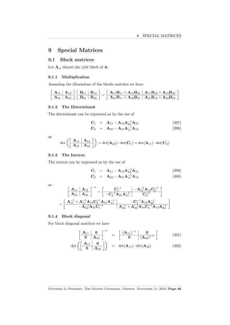
9.1 Block matrices

Let Aij denote the ijth block of A.

9.1.1 Multiplication

Assuming the dimensions of the blocks matches we have

A

11

A12

A21

A22

� B

11

B12

B21

B22

�=

A

11

B11

+A12

B21

A11

B12

+A12

B22

A21

B11

+A22

B21

A21

B12

+A22

B22

�

9.1.2 The Determinant

The determinant can be expressed as by the use of

C1

= A11

�A12

A�1

22

A21

(397)

C2

= A22

�A21

A�1

11

A12

(398)

as

det

✓A

11

A12

A21

A22

�◆= det(A

22

) · det(C1

) = det(A11

) · det(C2

)

9.1.3 The Inverse

The inverse can be expressed as by the use of

C1

= A11

�A12

A�1

22

A21

(399)

C2

= A22

�A21

A�1

11

A12

(400)

as A

11

A12

A21

A22

��1

=

C�1

1

�A�1

11

A12

C�1

2

�C�1

2

A21

A�1

11

C�1

2

�

=

A�1

11

+A�1

11

A12

C�1

2

A21

A�1

11

�C�1

1

A12

A�1

22

�A�1

22

A21

C�1

1

A�1

22

+A�1

22

A21

C�1

1

A12

A�1

22

�

9.1.4 Block diagonal

For block diagonal matrices we have

A

11

00 A

22

��1

=

(A

11

)�1 00 (A

22

)�1

�(401)

det

✓A

11

00 A

22

�◆= det(A

11

) · det(A22

) (402)


9.2 Discrete Fourier Transform Matrix, The 9 SPECIAL MATRICES

9.1.5 Schur complement

Regard the matrix A

11

A12

A21

A22

�

The Schur complement of block A11

of the matrix above is the matrix (denotedC

2

in the text above)A

22

�A21

A�1

11

A12

The Schur complement of block A22

of the matrix above is the matrix (denotedC

1

in the text above)A

11

�A12

A�1

22

A21

Using the Schur complement, one can rewrite the inverse of a block matrix

A

11

A12

A21

A22

��1

=

I 0

�A�1

22

A21

I

� (A

11

�A12

A�1

22

A21

)�1 00 A�1

22

� I �A

12

A�1

22

0 I

�

The Schur complement is useful when solving linear systems of the form

A

11

A12

A21

A22

� x1

x2

�=

b1

b2

�

which has the following equation for x1

(A11

�A12

A�1

22

A21

)x1

= b1

�A12

A�1

22

b2

When the appropriate inverses exists, this can be solved for x1

which can thenbe inserted in the equation for x

2

to solve for x2

.

9.2 Discrete Fourier Transform Matrix, The

The DFT matrix is an N ⇥N symmetric matrix WN , where the k, nth elementis given by

W knN = e

�j2⇡knN (403)

Thus the discrete Fourier transform (DFT) can be expressed as

X(k) =N�1X

n=0

x(n)W knN . (404)

Likewise the inverse discrete Fourier transform (IDFT) can be expressed as

x(n) =1

N

N�1X

k=0

X(k)W�knN . (405)

The DFT of the vector x = [x(0), x(1), · · · , x(N �1)]T can be written in matrixform as

X = WNx, (406)


9.3 Hermitian Matrices and skew-Hermitian 9 SPECIAL MATRICES

where X = [X(0), X(1), · · · , x(N � 1)]T . The IDFT is similarly given as

x = W�1

N X. (407)

Some properties of WN exist:

W�1

N =1

NW⇤

N (408)

WNW⇤N = NI (409)

W⇤N = WH

N (410)

If WN = e�j2⇡

N , then [23]

Wm+N/2N = �Wm

N (411)

Notice, the DFT matrix is a Vandermonde Matrix.The following important relation between the circulant matrix and the dis-

crete Fourier transform (DFT) exists

TC = W�1

N (I � (WNt))WN , (412)

where t = [t0

, t1

, · · · , tn�1

]T is the first row of TC .

9.3 Hermitian Matrices and skew-Hermitian

A matrix A 2 Cm⇥n is called Hermitian if

AH = A

For real valued matrices, Hermitian and symmetric matrices are equivalent.

A is Hermitian , xHAx 2 R, 8x 2 Cn⇥1 (413)

A is Hermitian , eig(A) 2 R (414)

Note thatA = B+ iC

where B,C are hermitian, then

B =A+AH

2, C =

A�AH

2i

9.3.1 Skew-Hermitian

A matrix A is called skew-hermitian if

A = �AH

For real valued matrices, skew-Hermitian and skew-symmetric matrices areequivalent.

A Hermitian , iA is skew-hermitian (415)

A skew-Hermitian , xHAy = �xHAHy, 8x,y (416)

A skew-Hermitian ) eig(A) = i�, � 2 R (417)


9.4 Idempotent Matrices 9 SPECIAL MATRICES

9.4 Idempotent Matrices

A matrix A is idempotent ifAA = A

Idempotent matrices A and B, have the following properties

An = A, forn = 1, 2, 3, ... (418)

I�A is idempotent (419)

AH is idempotent (420)

I�AH is idempotent (421)

If AB = BA ) AB is idempotent (422)

rank(A) = Tr(A) (423)

A(I�A) = 0 (424)

(I�A)A = 0 (425)

A+ = A (426)

f(sI+ tA) = (I�A)f(s) +Af(s+ t) (427)

Note that A� I is not necessarily idempotent.

9.4.1 Nilpotent

A matrix A is nilpotent ifA2 = 0

A nilpotent matrix has the following property:

f(sI+ tA) = If(s) + tAf 0(s) (428)

9.4.2 Unipotent

A matrix A is unipotent ifAA = I

A unipotent matrix has the following property:

f(sI+ tA) = [(I+A)f(s+ t) + (I�A)f(s� t)]/2 (429)

9.5 Orthogonal matrices

If a square matrix Q is orthogonal, if and only if,

QTQ = QQT = I

and then Q has the following properties

• Its eigenvalues are placed on the unit circle.

• Its eigenvectors are unitary, i.e. have length one.

• The inverse of an orthogonal matrix is orthogonal too.


9.6 Positive Definite and Semi-definite Matrices 9 SPECIAL MATRICES

Basic properties for the orthogonal matrix Q

Q�1 = QT

Q�T = Q

QQT = I

QTQ = I

det(Q) = ±1

9.5.1 Ortho-Sym

A matrix Q+

which simultaneously is orthogonal and symmetric is called anortho-sym matrix [20]. Hereby

QT+

Q+

= I (430)

Q+

= QT+

(431)

The powers of an ortho-sym matrix are given by the following rule

Qk+

=1 + (�1)k

2I+

1 + (�1)k+1

2Q

+

(432)

=1 + cos(k⇡)

2I+

1� cos(k⇡)

2Q

+

(433)

9.5.2 Ortho-Skew

A matrix which simultaneously is orthogonal and antisymmetric is called anortho-skew matrix [20]. Hereby

QH�Q� = I (434)

Q� = �QH� (435)

The powers of an ortho-skew matrix are given by the following rule

Qk� =

ik + (�i)k

2I� i

ik � (�i)k

2Q� (436)

= cos(k⇡

2)I+ sin(k

⇡

2)Q� (437)

9.5.3 Decomposition

A square matrix A can always be written as a sum of a symmetric A+

and anantisymmetric matrix A�

A = A+

+A� (438)

9.6 Positive Definite and Semi-definite Matrices

9.6.1 Definitions

A matrix A is positive definite if and only if

xTAx > 0, 8x 6= 0 (439)

A matrix A is positive semi-definite if and only if

xTAx � 0, 8x (440)

Note that if A is positive definite, then A is also positive semi-definite.


9.6 Positive Definite and Semi-definite Matrices 9 SPECIAL MATRICES

9.6.2 Eigenvalues

The following holds with respect to the eigenvalues:

A pos. def. , eig(A+A

H

2

) > 0

A pos. semi-def. , eig(A+A

H

2

) � 0(441)

9.6.3 Trace

The following holds with respect to the trace:

A pos. def. ) Tr(A) > 0A pos. semi-def. ) Tr(A) � 0

(442)

9.6.4 Inverse

If A is positive definite, then A is invertible and A�1 is also positive definite.

9.6.5 Diagonal

If A is positive definite, then Aii > 0, 8i

9.6.6 Decomposition I

The matrix A is positive semi-definite of rank r , there exists a matrix B ofrank r such that A = BBT

The matrix A is positive definite , there exists an invertible matrix B suchthat A = BBT

9.6.7 Decomposition II

Assume A is an n⇥ n positive semi-definite, then there exists an n⇥ r matrixB of rank r such that BTAB = I.

9.6.8 Equation with zeros

Assume A is positive semi-definite, then XTAX = 0 ) AX = 0

9.6.9 Rank of product

Assume A is positive definite, then rank(BABT ) = rank(B)

9.6.10 Positive definite property

If A is n⇥ n positive definite and B is r ⇥ n of rank r, then BABT is positivedefinite.

9.6.11 Outer Product

If X is n⇥ r, where n r and rank(X) = n, then XXT is positive definite.


9.7 Singleentry Matrix, The 9 SPECIAL MATRICES

9.6.12 Small pertubations

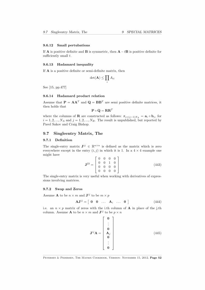
If A is positive definite and B is symmetric, then A� tB is positive definite forsu�ciently small t.

9.6.13 Hadamard inequality

If A is a positive definite or semi-definite matrix, then

det(A) Y

i

Aii

See [15, pp.477]

9.6.14 Hadamard product relation

Assume that P = AAT and Q = BBT are semi positive definite matrices, itthen holds that

P �Q = RRT

where the columns of R are constructed as follows: ri+(j�1)NA= ai � bj , for

i = 1, 2, ..., NA and j = 1, 2, ..., NB . The result is unpublished, but reported byPavel Sakov and Craig Bishop.

9.7 Singleentry Matrix, The

9.7.1 Definition

The single-entry matrix Jij 2 Rn⇥n is defined as the matrix which is zeroeverywhere except in the entry (i, j) in which it is 1. In a 4 ⇥ 4 example onemight have

J23 =

2

664

0 0 0 00 0 1 00 0 0 00 0 0 0

3

775 (443)

The single-entry matrix is very useful when working with derivatives of expres-sions involving matrices.

9.7.2 Swap and Zeros

Assume A to be n⇥m and Jij to be m⇥ p

AJij =⇥0 0 . . . Ai . . . 0

⇤(444)

i.e. an n ⇥ p matrix of zeros with the i.th column of A in place of the j.thcolumn. Assume A to be n⇥m and Jij to be p⇥ n

JijA =

2

66666666664

0...0Aj

0...0

3

77777777775

(445)


9.7 Singleentry Matrix, The 9 SPECIAL MATRICES

i.e. an p ⇥ m matrix of zeros with the j.th row of A in the placed of the i.throw.

9.7.3 Rewriting product of elements

AkiBjl = (AeieTj B)kl = (AJijB)kl (446)

AikBlj = (AT eieTj B

T )kl = (ATJijBT )kl (447)

AikBjl = (AT eieTj B)kl = (ATJijB)kl (448)

AkiBlj = (AeieTj B

T )kl = (AJijBT )kl (449)

9.7.4 Properties of the Singleentry Matrix

If i = jJijJij = Jij (Jij)T (Jij)T = Jij

Jij(Jij)T = Jij (Jij)TJij = Jij

If i 6= jJijJij = 0 (Jij)T (Jij)T = 0

Jij(Jij)T = Jii (Jij)TJij = Jjj

9.7.5 The Singleentry Matrix in Scalar Expressions

Assume A is n⇥m and J is m⇥ n, then

Tr(AJij) = Tr(JijA) = (AT )ij (450)

Assume A is n⇥ n, J is n⇥m and B is m⇥ n, then

Tr(AJijB) = (ATBT )ij (451)

Tr(AJjiB) = (BA)ij (452)

Tr(AJijJijB) = diag(ATBT )ij (453)

Assume A is n⇥ n, Jij is n⇥m B is m⇥ n, then

xTAJijBx = (ATxxTBT )ij (454)

xTAJijJijBx = diag(ATxxTBT )ij (455)

9.7.6 Structure Matrices

The structure matrix is defined by

@A

@Aij= Sij (456)

If A has no special structure then

Sij = Jij (457)

If A is symmetric thenSij = Jij + Jji � JijJij (458)


9.8 Symmetric, Skew-symmetric/Antisymmetric 9 SPECIAL MATRICES

9.8 Symmetric, Skew-symmetric/Antisymmetric

9.8.1 Symmetric

The matrix A is said to be symmetric if

A = AT (459)

Symmetric matrices have many important properties, e.g. that their eigenvaluesare real and eigenvectors orthogonal.

9.8.2 Skew-symmetric/Antisymmetric

The antisymmetric matrix is also known as the skew symmetric matrix. It hasthe following property from which it is defined

A = �AT (460)

Hereby, it can be seen that the antisymmetric matrices always have a zerodiagonal. The n⇥ n antisymmetric matrices also have the following properties.

det(AT ) = det(�A) = (�1)n det(A) (461)

� det(A) = det(�A) = 0, if n is odd (462)

The eigenvalues of an antisymmetric matrix are placed on the imaginary axisand the eigenvectors are unitary.

9.8.3 Decomposition

A square matrix A can always be written as a sum of a symmetric A+

and anantisymmetric matrix A�

A = A+

+A� (463)

Such a decomposition could e.g. be

A =A+AT

2+

A�AT

2= A

+

+A� (464)

9.9 Toeplitz Matrices

A Toeplitz matrix T is a matrix where the elements of each diagonal is thesame. In the n⇥ n square case, it has the following structure:

T =

2

66664

t11

t12

· · · t1n

t21

. . .. . .

......

. . .. . . t

12

tn1 · · · t21

t11

3

77775=

2

66664

t0

t1

· · · tn�1

t�1

. . .. . .

......

. . .. . . t

1

t�(n�1)

· · · t�1

t0

3

77775(465)

A Toeplitz matrix is persymmetric. If a matrix is persymmetric (or orthosym-metric), it means that the matrix is symmetric about its northeast-southwestdiagonal (anti-diagonal) [12]. Persymmetric matrices is a larger class of matri-ces, since a persymmetric matrix not necessarily has a Toeplitz structure. There


9.10 Transition matrices 9 SPECIAL MATRICES

are some special cases of Toeplitz matrices. The symmetric Toeplitz matrix isgiven by:

T =

2

66664

t0

t1

· · · tn�1

t1

. . .. . .

......

. . .. . . t

1

tn�1

· · · t1

t0

3

77775(466)

The circular Toeplitz matrix:

TC =

2

66664

t0

t1

· · · tn�1

tn�1

. . .. . .

......

. . .. . . t

1

t1

· · · tn�1

t0

3

77775(467)

The upper triangular Toeplitz matrix:

TU =

2

66664

t0

t1

· · · tn�1

0. . .

. . ....

.... . .

. . . t1

0 · · · 0 t0

3

77775, (468)

and the lower triangular Toeplitz matrix:

TL =

2

66664

t0

0 · · · 0

t�1

. . .. . .

......

. . .. . . 0

t�(n�1)

· · · t�1

t0

3

77775(469)

9.9.1 Properties of Toeplitz Matrices

The Toeplitz matrix has some computational advantages. The addition of twoToeplitz matrices can be done with O(n) flops, multiplication of two Toeplitzmatrices can be done in O(n lnn) flops. Toeplitz equation systems can be solvedin O(n2) flops. The inverse of a positive definite Toeplitz matrix can be foundin O(n2) flops too. The inverse of a Toeplitz matrix is persymmetric. Theproduct of two lower triangular Toeplitz matrices is a Toeplitz matrix. Moreinformation on Toeplitz matrices and circulant matrices can be found in [13, 7].

9.10 Transition matrices

A square matrix P is a transition matrix, also known as stochastic matrix orprobability matrix, if

0 (P)ij 1,X

j

(P)ij = 1

The transition matrix usually describes the probability of moving from state ito j in one step and is closely related to markov processes. Transition matrices


9.11 Units, Permutation and Shift 9 SPECIAL MATRICES

have the following properties

Prob[i ! j in 1 step] = (P)ij (470)

Prob[i ! j in 2 steps] = (P2)ij (471)

Prob[i ! j in k steps] = (Pk)ij (472)

If all rows are identical ) Pn = P (473)

↵P = ↵, ↵ is called invariant (474)

where ↵ is a so-called stationary probability vector, i.e., 0 ↵i 1 andP

i ↵i =1.

9.11 Units, Permutation and Shift

9.11.1 Unit vector

Let ei 2 Rn⇥1 be the ith unit vector, i.e. the vector which is zero in all entriesexcept the ith at which it is 1.

9.11.2 Rows and Columns

i.th row of A = eTi A (475)

j.th column of A = Aej (476)

9.11.3 Permutations

Let P be some permutation matrix, e.g.

P =

2

40 1 01 0 00 0 1

3

5 =⇥e2

e1

e3

⇤=

2

4eT2

eT1

eT3

3

5 (477)

For permutation matrices it holds that

PPT = I (478)

and that

AP =⇥Ae

2

Ae1

Ae3

⇤PA =

2

4eT2

AeT1

AeT3

A

3

5 (479)

That is, the first is a matrix which has columns of A but in permuted sequenceand the second is a matrix which has the rows of A but in the permuted se-quence.

9.11.4 Translation, Shift or Lag Operators

Let L denote the lag (or ’translation’ or ’shift’) operator defined on a 4 ⇥ 4example by

L =

2

664

0 0 0 01 0 0 00 1 0 00 0 1 0

3

775 (480)


9.12 Vandermonde Matrices 9 SPECIAL MATRICES

i.e. a matrix of zeros with one on the sub-diagonal, (L)ij = �i,j+1

. With somesignal xt for t = 1, ..., N , the n.th power of the lag operator shifts the indices,i.e.

(Lnx)t =n 0 for t = 1, .., n

xt�n for t = n+ 1, ..., N(481)

A related but slightly di↵erent matrix is the ’recurrent shifted’ operator definedon a 4x4 example by

L =

2

664

0 0 0 11 0 0 00 1 0 00 0 1 0

3

775 (482)

i.e. a matrix defined by (L)ij = �i,j+1

+ �i,1�j,dim(L)

. On a signal x it has thee↵ect

(Lnx)t = xt0 , t0 = [(t� n) mod N ] + 1 (483)

That is, L is like the shift operator L except that it ’wraps’ the signal as if itwas periodic and shifted (substituting the zeros with the rear end of the signal).Note that L is invertible and orthogonal, i.e.

L�1 = LT (484)

9.12 Vandermonde Matrices

A Vandermonde matrix has the form [15]

V =

2

6664

1 v1

v21

· · · vn�1

1

1 v2

v22

· · · vn�1

2

......

......

1 vn v2n · · · vn�1

n

3

7775. (485)

The transpose of V is also said to a Vandermonde matrix. The determinant isgiven by [29]

detV =Y

i>j

(vi � vj) (486)


10 FUNCTIONS AND OPERATORS

10 Functions and Operators

10.1 Functions and Series

10.1.1 Finite Series

(Xn � I)(X� I)�1 = I+X+X2 + ...+Xn�1 (487)

10.1.2 Taylor Expansion of Scalar Function

Consider some scalar function f(x) which takes the vector x as an argument.This we can Taylor expand around x

0

f(x) ⇠= f(x0

) + g(x0

)T (x� x0

) +1

2(x� x

0

)TH(x0

)(x� x0

) (488)

where

g(x0

) =@f(x)

@x

��x0

H(x0

) =@2f(x)

@x@xT

��x0

10.1.3 Matrix Functions by Infinite Series

As for analytical functions in one dimension, one can define a matrix functionfor square matrices X by an infinite series

f(X) =1X

n=0

cnXn (489)

assuming the limit exists and is finite. If the coe�cients cn fulfilsP

n cnxn < 1,

then one can prove that the above series exists and is finite, see [1]. Thus forany analytical function f(x) there exists a corresponding matrix function f(x)constructed by the Taylor expansion. Using this one can prove the followingresults:1) A matrix A is a zero of its own characteristic polynomium [1]:

p(�) = det(I��A) =X

n

cn�n ) p(A) = 0 (490)

2) If A is square it holds that [1]

A = UBU�1 ) f(A) = Uf(B)U�1 (491)

3) A useful fact when using power series is that

An ! 0forn ! 1 if |A| < 1 (492)

10.1.4 Identity and commutations

It holds for an analytical matrix function f(X) that

f(AB)A = Af(BA) (493)

see B.1.2 for a proof.


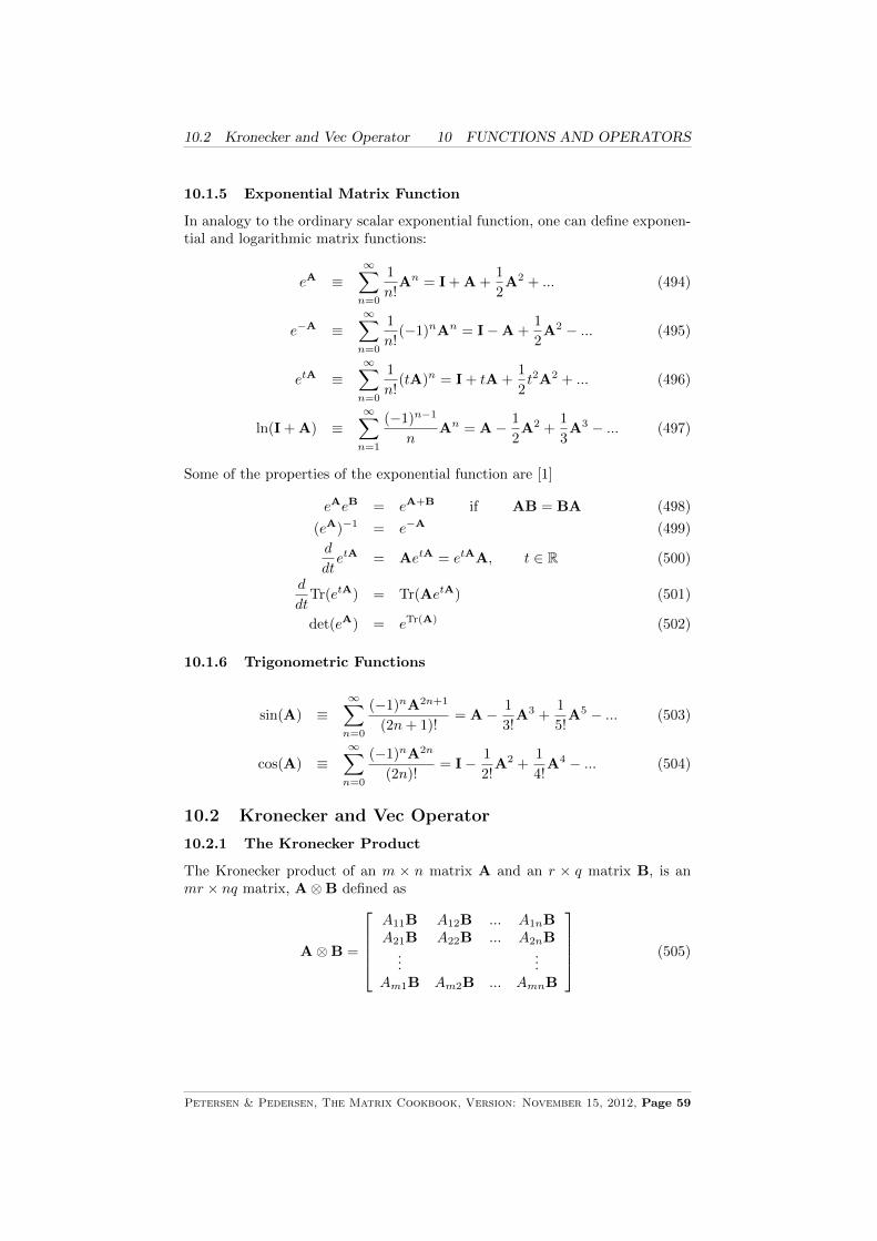
10.2 Kronecker and Vec Operator 10 FUNCTIONS AND OPERATORS

10.1.5 Exponential Matrix Function

In analogy to the ordinary scalar exponential function, one can define exponen-tial and logarithmic matrix functions:

eA ⌘1X

n=0

1

n!An = I+A+

1

2A2 + ... (494)

e�A ⌘1X

n=0

1

n!(�1)nAn = I�A+

1

2A2 � ... (495)

etA ⌘1X

n=0

1

n!(tA)n = I+ tA+

1

2t2A2 + ... (496)

ln(I+A) ⌘1X

n=1

(�1)n�1

nAn = A� 1

2A2 +

1

3A3 � ... (497)

Some of the properties of the exponential function are [1]

eAeB = eA+B if AB = BA (498)

(eA)�1 = e�A (499)

d

dtetA = AetA = etAA, t 2 R (500)

d

dtTr(etA) = Tr(AetA) (501)

det(eA) = eTr(A) (502)

10.1.6 Trigonometric Functions

sin(A) ⌘1X

n=0

(�1)nA2n+1

(2n+ 1)!= A� 1

3!A3 +

1

5!A5 � ... (503)

cos(A) ⌘1X

n=0

(�1)nA2n

(2n)!= I� 1

2!A2 +

1

4!A4 � ... (504)

10.2 Kronecker and Vec Operator

10.2.1 The Kronecker Product

The Kronecker product of an m ⇥ n matrix A and an r ⇥ q matrix B, is anmr ⇥ nq matrix, A⌦B defined as

A⌦B =

2

6664

A11

B A12

B ... A1nB

A21

B A22

B ... A2nB

......

Am1

B Am2

B ... AmnB

3

7775(505)


10.2 Kronecker and Vec Operator 10 FUNCTIONS AND OPERATORS

The Kronecker product has the following properties (see [19])

A⌦ (B+C) = A⌦B+A⌦C (506)

A⌦B 6= B⌦A in general (507)

A⌦ (B⌦C) = (A⌦B)⌦C (508)

(↵AA⌦ ↵BB) = ↵A↵B(A⌦B) (509)

(A⌦B)T = AT ⌦BT (510)

(A⌦B)(C⌦D) = AC⌦BD (511)

(A⌦B)�1 = A�1 ⌦B�1 (512)

(A⌦B)+ = A+ ⌦B+ (513)

rank(A⌦B) = rank(A)rank(B) (514)

Tr(A⌦B) = Tr(A)Tr(B) = Tr(⇤A ⌦⇤B) (515)

det(A⌦B) = det(A)rank(B) det(B)rank(A) (516)

{eig(A⌦B)} = {eig(B⌦A)} if A,B are square (517)

{eig(A⌦B)} = {eig(A)eig(B)T } (518)

if A,B are symmetric and square

eig(A⌦B) = eig(A)⌦ eig(B) (519)

Where {�i} denotes the set of values �i, that is, the values in no particularorder or structure, and ⇤A denotes the diagonal matrix with the eigenvalues ofA.

10.2.2 The Vec Operator

The vec-operator applied on a matrix A stacks the columns into a vector, i.e.for a 2⇥ 2 matrix

A =

A

11

A12

A21

A22

�vec(A) =

2

664

A11

A21

A12

A22

3

775

Properties of the vec-operator include (see [19])

vec(AXB) = (BT ⌦A)vec(X) (520)

Tr(ATB) = vec(A)T vec(B) (521)

vec(A+B) = vec(A) + vec(B) (522)

vec(↵A) = ↵ · vec(A) (523)

aTXBXT c = vec(X)T (B⌦ caT )vec(X) (524)

See B.1.1 for a proof for Eq. 524.


10.3 Vector Norms 10 FUNCTIONS AND OPERATORS

10.3 Vector Norms

10.3.1 Examples

||x||1

=X

i

|xi| (525)

||x||22

= xHx (526)

||x||p =

"X

i

|xi|p#1/p

(527)

||x||1 = maxi

|xi| (528)

Further reading in e.g. [12, p. 52]

10.4 Matrix Norms

10.4.1 Definitions

A matrix norm is a mapping which fulfils

||A|| � 0 (529)

||A|| = 0 , A = 0 (530)

||cA|| = |c|||A||, c 2 R (531)

||A+B|| ||A||+ ||B|| (532)

10.4.2 Induced Norm or Operator Norm

An induced norm is a matrix norm induced by a vector norm by the following

||A|| = sup{||Ax|| | ||x|| = 1} (533)

where || · || on the left side is the induced matrix norm, while || · || on the rightside denotes the vector norm. For induced norms it holds that

||I|| = 1 (534)||Ax|| ||A|| · ||x||, for all A,x (535)||AB|| ||A|| · ||B||, for all A,B (536)

10.4.3 Examples

||A||1

= maxj

X

i

|Aij | (537)

||A||2

=qmax eig(AHA) (538)

||A||p = ( max||x||p=1

||Ax||p)1/p (539)

||A||1 = maxi

X

j

|Aij | (540)

||A||F

=

sX

ij

|Aij |2 =qTr(AAH) (Frobenius) (541)


10.5 Rank 10 FUNCTIONS AND OPERATORS

||A||max

= maxij

|Aij | (542)

||A||KF

= ||sing(A)||1

(Ky Fan) (543)

where sing(A) is the vector of singular values of the matrix A.

10.4.4 Inequalities

E. H. Rasmussen has in yet unpublished material derived and collected thefollowing inequalities. They are collected in a table as below, assuming A is anm⇥ n, and d = rank(A)

||A||max

||A||1

||A||1 ||A||2

||A||F

||A||KF

||A||max

1 1 1 1 1||A||

1

m mpm

pm

pm

||A||1 n npn

pn

pn

||A||2

pmn

pn

pm 1 1

||A||F

pmn

pn

pm

pd 1

||A||KF

pmnd

pnd

pmd d

pd

which are to be read as, e.g.

||A||2

pm · ||A||1 (544)

10.4.5 Condition Number

The 2-norm of A equalsp(max(eig(ATA))) [12, p.57]. For a symmetric, pos-

itive definite matrix, this reduces to max(eig(A)) The condition number basedon the 2-norm thus reduces to

kAk2

kA�1k2

= max(eig(A))max(eig(A�1)) =max(eig(A))

min(eig(A)). (545)

10.5 Rank

10.5.1 Sylvester’s Inequality

If A is m⇥ n and B is n⇥ r, then

rank(A) + rank(B)� n rank(AB) min{rank(A), rank(B)} (546)

10.6 Integral Involving Dirac Delta Functions

Assuming A to be square, thenZ

p(s)�(x�As)ds =1

det(A)p(A�1x) (547)

Assuming A to be ”underdetermined”, i.e. ”tall”, then

Zp(s)�(x�As)ds =

(1p

det(A

TA)

p(A+x) if x = AA+x

0 elsewhere

)(548)

See [9].


10.7 Miscellaneous 10 FUNCTIONS AND OPERATORS

10.7 Miscellaneous

For any A it holds that

rank(A) = rank(AT ) = rank(AAT ) = rank(ATA) (549)

It holds that

A is positive definite , 9B invertible, such that A = BBT (550)


A ONE-DIMENSIONAL RESULTS

A One-dimensional Results

A.1 Gaussian

A.1.1 Density

p(x) =1p2⇡�2

exp

✓� (x� µ)2

2�2

◆(551)

A.1.2 NormalizationZe�

(s�µ)2

2�2 ds =p2⇡�2 (552)

Ze�(ax2

+bx+c)dx =

r⇡

aexp

b2 � 4ac

4a

�(553)

Zec2x

2+c1x+c0dx =

r⇡

�c2

exp

c21

� 4c2

c0

�4c2

�(554)

A.1.3 Derivatives@p(x)

@µ= p(x)

(x� µ)

�2

(555)

@ ln p(x)

@µ=

(x� µ)

�2

(556)

@p(x)

@�= p(x)

1

�

(x� µ)2

�2

� 1

�(557)

@ ln p(x)

@�=

1

�

(x� µ)2

�2

� 1

�(558)

A.1.4 Completing the Squares

c2

x2 + c1

x+ c0

= �a(x� b)2 + w

�a = c2

b =1

2

c1

c2

w =1

4

c21

c2

+ c0

or

c2

x2 + c1

x+ c0

= � 1

2�2

(x� µ)2 + d

µ =�c

1

2c2

�2 =�1

2c2

d = c0

� c21

4c2

A.1.5 Moments

If the density is expressed by

p(x) =1p2⇡�2

exp

� (s� µ)2

2�2

�or p(x) = C exp(c

2

x2 + c1

x) (559)

then the first few basic moments are


A.2 One Dimensional Mixture of GaussiansA ONE-DIMENSIONAL RESULTS

hxi = µ = �c12c2

hx2i = �2 + µ2 = �1

2c2+⇣

�c12c2

⌘2

hx3i = 3�2µ+ µ3 = c1(2c2)2

h3� c21

2c2

i

hx4i = µ4 + 6µ2�2 + 3�4 =⇣

c12c2

⌘4

+ 6⇣

c12c2

⌘2

⇣�1

2c2

⌘+ 3

⇣1

2c2

⌘2

and the central moments are

h(x� µ)i = 0 = 0

h(x� µ)2i = �2 =h�1

2c2

i

h(x� µ)3i = 0 = 0

h(x� µ)4i = 3�4 = 3h

1

2c2

i2

A kind of pseudo-moments (un-normalized integrals) can easily be derived as

Zexp(c

2

x2 + c1

x)xndx = Zhxni =r

⇡

�c2

exp

c21

�4c2

�hxni (560)

¿From the un-centralized moments one can derive other entities like

hx2i � hxi2 = �2 = �1

2c2hx3i � hx2ihxi = 2�2µ = 2c1(2c2)2

hx4i � hx2i2 = 2�4 + 4µ2�2 = 2

(2c2)2

h1� 4 c21

2c2

i

A.2 One Dimensional Mixture of Gaussians

A.2.1 Density and Normalization

p(s) =KX

k

⇢kp2⇡�2

k

exp

�1

2

(s� µk)2

�2

k

�(561)

A.2.2 Moments

A useful fact of MoG, is that

hxni =X

k

⇢khxnik (562)

where h·ik denotes average with respect to the k.th component. We can calculatethe first four moments from the densities

p(x) =X

k

⇢k1p2⇡�2

k

exp

�1

2

(x� µk)2

�2

k

�(563)

p(x) =X

k

⇢kCk exp⇥ck2x

2 + ck1x⇤

(564)

as


B PROOFS AND DETAILS

hxi =P

k ⇢kµk =P

k ⇢k

h�ck12ck2

i

hx2i =P

k ⇢k(�2

k + µ2

k) =P

k ⇢k

�1

2ck2+⇣

�ck12ck2

⌘2

�

hx3i =P

k ⇢k(3�2

kµk + µ3

k) =P

k ⇢k

hck1

(2ck2)2

h3� c2k1

2ck2

ii

hx4i =P

k ⇢k(µ4

k + 6µ2

k�2

k + 3�4

k) =P

k ⇢k

⇣1

2ck2

⌘2

⇣ck12ck2

⌘2

� 6 c2k12ck2

+ 3

��

If all the gaussians are centered, i.e. µk = 0 for all k, then

hxi = 0 = 0

hx2i =P

k ⇢k�2

k =P

k ⇢k

h�1

2ck2

i

hx3i = 0 = 0

hx4i =P

k ⇢k3�4

k =P

k ⇢k3h

�1

2ck2

i2

¿From the un-centralized moments one can derive other entities like

hx2i � hxi2 =P

k,k0 ⇢k⇢k0⇥µ2

k + �2

k � µkµk0⇤

hx3i � hx2ihxi =P

k,k0 ⇢k⇢k0⇥3�2

kµk + µ3

k � (�2

k + µ2

k)µk0⇤

hx4i � hx2i2 =P

k,k0 ⇢k⇢k0⇥µ4

k + 6µ2

k�2

k + 3�4

k � (�2

k + µ2

k)(�2

k0 + µ2

k0)⇤

A.2.3 Derivatives

Defining p(s) =P

k ⇢kNs(µk,�2

k) we get for a parameter ✓j of the j.th compo-nent

@ ln p(s)

@✓j=

⇢jNs(µj ,�2

j )Pk ⇢kNs(µk,�2

k)

@ ln(⇢jNs(µj ,�2

j ))

@✓j(565)

that is,

@ ln p(s)

@⇢j=

⇢jNs(µj ,�2


k)

1

⇢j(566)

@ ln p(s)

@µj=

⇢jNs(µj ,�2


k)

(s� µj)

�2

j

(567)

@ ln p(s)

@�j=

⇢jNs(µj ,�2


k)

1

�j

"(s� µj)2

�2

j

� 1

#(568)

Note that ⇢k must be constrained to be proper ratios. Defining the ratios by⇢j = erj/

Pk e

rk , we obtain

@ ln p(s)

@rj=X

l

@ ln p(s)

@⇢l

@⇢l@rj

where@⇢l@rj

= ⇢l(�lj � ⇢j) (569)

B Proofs and Details

B.1 Misc Proofs

B.1.1 Proof of Equation 524

The following proof is work of Florian Roemer. Note the the vectors and ma-trices below can be complex and the notation XH is used for transpose andconjugated, while XT is only transpose of the complex matrix.


B.1 Misc Proofs B PROOFS AND DETAILS

Define the row vector y = aHXB and the column vector z = XHc. Then

aTXBXT c = yz = zTyT

Note that y can be rewritten as vec(y)T which is the same as

vec(conj(y))H = vec(aT conj(X)conj(B))H

where ”conj” means complex conjugated. Applying the vec rule for linear formsEq 520, we get

y = (BH ⌦ aT vec(conj(X))H = vec(X)T (B⌦ conj(a))

where we have also used the rule for transpose of Kronecker products. For yT

this yields (BT ⌦ aH)vec(X). Similarly we can rewrite z which is the same asvec(zT ) = vec(cT conj(X)). Applying again Eq 520, we get

z = (I⌦ cT )vec(conj(X))

where I is the identity matrix. For zT we obtain vec(X)(I ⌦ c). Finally, theoriginal expression is zTyT which now takes the form

vec(X)H(I⌦ c)(BT ⌦ aH)vec(X)

the final step is to apply the rule for products of Kronecker products and bythat combine the Kronecker products. This gives

vec(X)H(BT ⌦ caH)vec(X)

which is the desired result.


For any analytical function f(X) of a matrix argument X, it holds that

f(AB)A =

1X

n=0

cn(AB)n!A

=1X

n=0

cn(AB)nA

=1X

n=0

cnA(BA)n

= A1X

n=0

cn(BA)n

= Af(BA)


Essentially we need to calculate



@(Xn)kl@Xij

=@

@Xij

X

u1,...,un�1

Xk,u1Xu1,u2 ...Xun�1,l

= �k,i�u1,jXu1,u2 ...Xun�1,l

+Xk,u1�u1,i�u2,j ...Xun�1,l

...

+Xk,u1Xu1,u2 ...�un�1,i�l,j

=n�1X

r=0

(Xr)ki(Xn�1�r)jl

=n�1X

r=0

(XrJijXn�1�r)kl

Using the properties of the single entry matrix found in Sec. 9.7.4, the resultfollows easily.

B.1.4 Details on Eq. 571

@ det(XHAX) = det(XHAX)Tr[(XHAX)�1@(XHAX)]

= det(XHAX)Tr[(XHAX)�1(@(XH)AX+XH@(AX))]

= det(XHAX)�Tr[(XHAX)�1@(XH)AX]

+Tr[(XHAX)�1XH@(AX)]�

= det(XHAX)�Tr[AX(XHAX)�1@(XH)]

+Tr[(XHAX)�1XHA@(X)]�

First, the derivative is found with respect to the real part of X

@ det(XHAX)

@<X = det(XHAX)⇣Tr[AX(XHAX)�1@(XH)]

@<X+Tr[(XHAX)�1XHA@(X)]

@<X⌘

= det(XHAX)�AX(XHAX)�1 + ((XHAX)�1XHA)T

�

Through the calculations, (100) and (240) were used. In addition, by use of(241), the derivative is found with respect to the imaginary part of X

i@ det(XHAX)

@=X = i det(XHAX)⇣Tr[AX(XHAX)�1@(XH)]

@=X+Tr[(XHAX)�1XHA@(X)]

@=X⌘

= det(XHAX)�AX(XHAX)�1 � ((XHAX)�1XHA)T

�

Hence, derivative yields

@ det(XHAX)

@X=

1

2

⇣@ det(XHAX)

@<X � i@ det(XHAX)

@=X⌘

= det(XHAX)�(XHAX)�1XHA

�T



and the complex conjugate derivative yields

@ det(XHAX)

@X⇤ =1

2

⇣@ det(XHAX)

@<X + i@ det(XHAX)

@=X⌘

= det(XHAX)AX(XHAX)�1

Notice, for real X, A, the sum of (249) and (250) is reduced to (54).Similar calculations yield

@ det(XAXH)

@X=

1

2

⇣@ det(XAXH)

@<X � i@ det(XAXH)

@=X⌘

= det(XAXH)�AXH(XAXH)�1

�T(570)

and

@ det(XAXH)

@X⇤ =1

2

⇣@ det(XAXH)

@<X + i@ det(XAXH)

@=X⌘

= det(XAXH)(XAXH)�1XA (571)


REFERENCES REFERENCES

References

[1] Karl Gustav Andersson and Lars-Christer Boiers. Ordinaera di↵erentialek-vationer. Studenterlitteratur, 1992.

[2] Jorn Anemuller, Terrence J. Sejnowski, and Scott Makeig. Complex inde-pendent component analysis of frequency-domain electroencephalographicdata. Neural Networks, 16(9):1311–1323, November 2003.

[3] S. Barnet. Matrices. Methods and Applications. Oxford Applied Mathe-matics and Computin Science Series. Clarendon Press, 1990.

[4] Christopher Bishop. Neural Networks for Pattern Recognition. OxfordUniversity Press, 1995.

[5] Robert J. Boik. Lecture notes: Statistics 550. Online, April 22 2002. Notes.

[6] D. H. Brandwood. A complex gradient operator and its application inadaptive array theory. IEE Proceedings, 130(1):11–16, February 1983. PTS.F and H.

[7] M. Brookes. Matrix Reference Manual, 2004. Website May 20, 2004.

[8] Contradsen K., En introduktion til statistik, IMM lecture notes, 1984.

[9] Mads Dyrholm. Some matrix results, 2004. Website August 23, 2004.

[10] Nielsen F. A., Formula, Neuro Research Unit and Technical university ofDenmark, 2002.

[11] Gelman A. B., J. S. Carlin, H. S. Stern, D. B. Rubin, Bayesian DataAnalysis, Chapman and Hall / CRC, 1995.

[12] Gene H. Golub and Charles F. van Loan. Matrix Computations. The JohnsHopkins University Press, Baltimore, 3rd edition, 1996.

[13] Robert M. Gray. Toeplitz and circulant matrices: A review. Technicalreport, Information Systems Laboratory, Department of Electrical Engi-neering,Stanford University, Stanford, California 94305, August 2002.

[14] Simon Haykin. Adaptive Filter Theory. Prentice Hall, Upper Saddle River,NJ, 4th edition, 2002.

[15] Roger A. Horn and Charles R. Johnson. Matrix Analysis. CambridgeUniversity Press, 1985.

[16] Mardia K. V., J.T. Kent and J.M. Bibby, Multivariate Analysis, AcademicPress Ltd., 1979.

[17] Mathpages on ”Eigenvalue Problems and Matrix Invariants”,

http://www.mathpages.com/home/kmath128.htm

[18] Carl D. Meyer. Generalized inversion of modified matrices. SIAM Journalof Applied Mathematics, 24(3):315–323, May 1973.


REFERENCES REFERENCES

[19] Thomas P. Minka. Old and new matrix algebra useful for statistics, De-cember 2000. Notes.

[20] Daniele Mortari Ortho–Skew and Ortho–Sym Matrix Trigonometry JohnLee Junkins Astrodynamics Symposium, AAS 03–265, May 2003. TexasA&M University, College Station, TX

[21] L. Parra and C. Spence. Convolutive blind separation of non-stationarysources. In IEEE Transactions Speech and Audio Processing, pages 320–327, May 2000.

[22] Kaare Brandt Petersen, Jiucang Hao, and Te-Won Lee. Generative andfiltering approaches for overcomplete representations. Neural InformationProcessing - Letters and Reviews, vol. 8(1), 2005.

[23] John G. Proakis and Dimitris G. Manolakis. Digital Signal Processing.Prentice-Hall, 1996.

[24] Laurent Schwartz. Cours d’Analyse, volume II. Hermann, Paris, 1967. Asreferenced in [14].

[25] Shayle R. Searle. Matrix Algebra Useful for Statistics. John Wiley andSons, 1982.

[26] G. Seber and A. Lee. Linear Regression Analysis. John Wiley and Sons,2002.

[27] S. M. Selby. Standard Mathematical Tables. CRC Press, 1974.

[28] Inna Stainvas. Matrix algebra in di↵erential calculus. Neural ComputingResearch Group, Information Engeneering, Aston University, UK, August2002. Notes.

[29] P. P. Vaidyanathan. Multirate Systems and Filter Banks. Prentice Hall,1993.

[30] Max Welling. The Kalman Filter. Lecture Note.

[31] Wikipedia on minors: ”Minor (linear algebra)”,

http://en.wikipedia.org/wiki/Minor_(linear_algebra)

[32] Zhaoshui He, Shengli Xie, et al, ”Convolutive blind source separation infrequency domain based on sparse representation”, IEEE Transactions onAudio, Speech and Language Processing, vol.15(5):1551-1563, July 2007.

[33] Karim T. Abou-Moustafa On Derivatives of Eigenvalues and Eigenvectorsof the Generalized Eigenvalue Problem. McGill Technical Report, October2010.

[34] Mohammad Emtiyaz Khan Updating Inverse of a Matrix When a Columnis Added/Removed. Emt CS,UBC February 27, 2008


Index

Anti-symmetric, 54

Block matrix, 46

Chain rule, 15Cholesky-decomposition, 32Co-kurtosis, 34Co-skewness, 34Condition number, 62Cramers Rule, 29

Derivative of a complex matrix, 24Derivative of a determinant, 8Derivative of a trace, 12Derivative of an inverse, 9Derivative of symmetric matrix, 15Derivatives of Toeplitz matrix, 16Dirichlet distribution, 37

Eigenvalues, 30Eigenvectors, 30Exponential Matrix Function, 59

Gaussian, conditional, 40Gaussian, entropy, 44Gaussian, linear combination, 41Gaussian, marginal, 40Gaussian, product of densities, 42Generalized inverse, 21

Hadamard inequality, 52Hermitian, 48

Idempotent, 49

Kronecker product, 59

LDL decomposition, 33LDM-decomposition, 33Linear regression, 28LU decomposition, 32Lyapunov Equation, 30

Moore-Penrose inverse, 21Multinomial distribution, 37

Nilpotent, 49Norm of a matrix, 61Norm of a vector, 61

Normal-Inverse Gamma distribution, 37Normal-Inverse Wishart distribution, 39

Orthogonal, 49

Power series of matrices, 58Probability matrix, 55Pseudo-inverse, 21

Schur complement, 41, 47Single entry matrix, 52Singular Valued Decomposition (SVD),

31Skew-Hermitian, 48Skew-symmetric, 54Stochastic matrix, 55Student-t, 37Sylvester’s Inequality, 62Symmetric, 54

Taylor expansion, 58Toeplitz matrix, 54Transition matrix, 55Trigonometric functions, 59

Unipotent, 49

Vandermonde matrix, 57Vec operator, 59, 60

Wishart distribution, 38Woodbury identity, 18

72

the matrix cookbook - university of waterloo

Documents