the matrix multidisk problem
TRANSCRIPT
Integr. equ. oper. theory 46 (2003) 285–3390378-620X/030285-55, DOI 10.1007/s00020-002-1142-7c© 2003 Birkhauser Verlag Basel/Switzerland
Integral Equationsand Operator Theory
The Matrix Multidisk Problem
Harry Dym and J. William Helton
Abstract. The solutions of a class of matrix optimization problems (includingthe Nehari problem and its multidisk generalization) can be identified withthe solutions of an abstract operator equation of the form T (·, ·, ·) = 0 . Thisequation can be can be solved numerically by Newton’s method if the differen-tial T ′ of T is invertible at the points of interest. This is typically too difficultto verify. However, it turns out that under reasonably broad conditions wecan identify T ′ as the sum of a block Toeplitz operator and a compact blockHankel operator. Moreover, we can show that the block Toeplitz operator isa Fredholm operator and and in some cases can calculate its Fredholm index.Thus, T ′ will also be a Fredholm operator of the same index. In a number ofcases that have been checked todate, numerical methods perform well whenthe Fredholm index is equal to to zero and poorly otherwise. The main focusof this paper is on the multidisk problem alluded to above. However, a numberof analogies with existing work on matrix optimization have been worked outand incorporated.
Mathematics Subject Classification (2000). Primary 47B35, Secondary 49K30.
Keywords. The Matrix Multidisk Problem.
1. Introduction
A number of basic problems in operator theory can be incorporated in the frame-work of the following matrix optimization problem, that we shall refer to as theMOPT problem:
Given a smooth, positive semi-definite (and hence selfadjoint), m×m-matrix val-ued function Γ(eiθ, z) of eiθ ∈ T , z = (z1, . . . , zN ) ∈ C
N and z = (z1, . . . , zN ) ∈C
N , find f∗ ∈ AN and γ∗ > 0 such that
γ∗=supθ
‖Γ(eiθ, f∗(eiθ))‖m×m = inff∈AN
supθ
‖Γ(eiθ, f(eiθ))‖m×m .
H. Dym thanks Renee and Jay Weiss for endowing the chair that supports his research. Thanksare also extended to NSF, ONR, DARPA, and the Ford Motor Co. for partial support.
286 Dym and Helton IEOT
Here ‖ · ‖m×m denotes the operator norm (i.e., the largest singular value) and
AN is a prescribed class of functions (f1, . . . , fN ) that are analytic in the openunit disk D . It is important to keep in mind that while Γ is smooth, the matrixnorm ‖Γ(eiθ, z)‖m×m is not. (Think of |x| .) Examples of the MOPT problem willbe furnished below. Under reasonable assumptions the solutions of this problemcan be identified with the solutions of an abstract operator equation of the formT (·, ·, ·) = 0 . This equation can be can be solved numerically by Newton’s methodor variations thereof, providing that the differential T ′ of T is invertible at thepoints of interest. This is typically too difficult to verify. However, it turns outthat under reasonably broad conditions we can identify T ′ as the sum of a blockToeplitz operator and a compact block Hankel operator. Moreover, we can showthat the block Toeplitz operator is a Fredholm operator and and in some casescan calculate its Fredholm index. Thus, T ′ will also be a Fredholm operator ofthe same index. In a number of cases that have been checked todate, numericalmethods perform well when the Fredholm index is equal to to zero and poorlyotherwise. Thus checking whether or not the differential is a Fredholm operatorwith Fredholm index zero seems to be an effective practical test for the efficiencyof the two algorithms that have been investigated so far in this framework. Thefact that we now have two different yet successful examples of how to calculateand use the Fredholm index 0 test suggests that this method is applicable to awide range of problems.
To help describe the issues under study we shall first present a number ofexamples of the MOPT problem. We shall then discuss our methodology in generalterms and, subsequently, we shall analyze in detail the second of the two algorithmsalluded to above. The first was considered in detail in [DHM:02]. The analysis inthe present paper is somewhat cleaner. In addition, a number of analogies withexisting work on matrix optimization have been worked out and incorporated.
1.1. Some illustrative problems
There are basically two classes of problems under consideration: θ dependent andθ independent. The former all fall under the general category of multidisk prob-lems, the simplest of which (i.e., the one-disk problem) coincides with the Nehariproblem. The latter are matrix problems in finite dimensional Euclidean space andin some sense could have served as a model for the more complicated θ dependentproblems, though chronologically, thats not the way this paper developed. Ourmain focus in this paper, however, is on θ dependent problems.
1.1.1. The matrix Nehari problem The given data is a bounded m×m matrixvalued function K, on the unit circle T , and the objective is to find its distanceto the Hardy space of bounded matrix valued analytic functions H∞
m×m. That is,with some poetic license1, we wish to find
dist(K, H∞m×m) := inf
F∈H∞m×m
supθ
‖ K(eiθ) − F (eiθ) ‖m×m. (1.1)
1We are using supremum instead of essential supremum.
Vol. 46 (2003) Matrix Multidisk Problem 287
Since ‖BBT ‖m×m = ‖B‖2m×m for any m×m matrix B and its conjugate transpose
BT , we may rewrite (1.1) as
dist(K, H∞m×m)2 = inf
F∈H∞m×m
supθ
‖(K(eiθ)−F (eiθ))(K(eiθ)−F (eiθ))T ‖m×m. (1.2)
To put the Nehari Problem in MOPT notation, take
Γ(eiθ, Z) = (K(eiθ) − Z)(K(eiθ) − Z)T , (1.3)
where Z = (zij)mi,j=1 denotes a matrix with N = m2 independent entries. It is
clear that Γ(eiθ, Z) is analytic in zij and zij , i, j = 1, . . . , m, and continuous in θif K is continuous in θ, and that in this case MOPT gives an optimal value γ suchthat
γ = dist(K, H∞m×m)2. (1.4)
Also, in view of the convexity of the L∞m×m norm, a local solution is a global
solution too. Hence solutions to MOPT correspond to solutions to the Nehariproblem: the minimizers f ∈ H∞
m×m are the same, while the optimal values arerelated by equation (1.4).
Remark 1.1. The factorization in formula (1.3) is in the opposite order from thatused in [DHM:02]. The reason for this choice is discussed in Section 3.3.
1.1.2. The multidisk problem The v-disk problem is a natural generalizationof the Nehari problem (which we look at as a one disk problem) to “v-disks”. Givena set K1, . . . , Kv of continuous m × m matrix valued functions on the unit circle(which we think of as the centers of matrix function disks) and v performancefunctions
Γp(eiθ, Z) = (Kp(eiθ) − Z)(Kp(eiθ) − Z)T , p = 1, . . . , v, (1.5)
the v-disk problem is to find the smallest number γ and a function f in the spaceof bounded analytic functions H∞
m×m, so that
Γp(eiθ, f(eiθ)) ≤ γIm
for p = 1, . . . , v and all θ. The multidisk problem for v disks is the MOPT problemfor the performance function
Γ := diag(Γ1, . . . ,Γv) =
Γ1 0 . . . 00 Γ2 . . . 0...
.... . .
...0 0 . . . Γv
, (1.6)
where Γp, p = 1, . . . , v, is given by (1.5).
288 Dym and Helton IEOT
1.1.3. Matrix optimization: the θ independent case In the θ independentcase, the performance function Γ(eiθ, z) depends only upon z but not upon θ. Abasic problem that falls into this category is to find
γ∗ = minx1,...,xn∈R
‖(C −N∑
j=1
xjAj)2‖, (1.7)
where C and Aj , j = 1, . . . , N , are real symmetric matrices. This is an MOPTproblem with
Γ(eiθ, z) = (C −N∑
j=1
xjAj)2 (1.8)
andzj = xj + iyj , j = 1, . . . , N.
Note that Γ is independent of eiθ.
1.1.4. Another θ independent matrix optimization problem Anotherproblem we consider is to find
γ∗ = minx1,...,xn∈R
eigenvalue{C −N∑
j=1
xjAj}, (1.9)
where C and Aj , j = 1, . . . , N , are real symmetric matrices. This looks like an anMOPT problem with
Γ(eiθ, z) = C −N∑
j=1
xjAj (1.10)
andzj = xj + iyj , j = 1, . . . , N.
However, there is one important difference: Γ(eiθ, z) is selfadjoint but not positivesemidefinite. Nevertheless, much of the analysis goes through and will be discussedin detail in Section 6.
The problems in Sections 1.1.3 and 1.1.4 are semidefinite programing matrixoptimization problem similar to those which are very popular in engineering circles.Our results (in Sections 5 and 6) on the efficiency of numerical schemes closelyparallel those of [AHO:98]. A number of results from the latter paper are reprovedby the methods of this paper in Section 7.
1.1.5. Supplementary references In this subsection we list a number of pa-pers that explore issues along the lines of the examples furnished above and somerelated issues. A comprehensive analysis of the Nehari problem in both the matrixand operator cases is developed in a series of papers by Adamyan, Arov and Krein;see e.g., [AAK:68]-[AAK:71b] for the most recent in the series and references tothe others, and [Pe:98] for a useful recent survey. State space approaches to matrixversions of this class of problems have been pursued since the early eighties. Tworecent references which give good coverage of the present state of the art (as well
Vol. 46 (2003) Matrix Multidisk Problem 289
as the art of the state) are the monographs [ZDG:96] by Zhou, Doyle and Gloverand [GL:95] by Limebeer and Green. Another good source on state space meth-ods for the Nehari problem and bitangential interpolation problems is the book[BGK:90] by Ball, Gohberg and Rodman. A different approach based on liftingtheorems is discussed extensively in the book [FF:90] of Foias and Frazo. For ananalysis in the setting of the Wiener algebra, see the papers [DG:83], [DG:86]. Thediscussion and and the surveys provided in [Dy:89] and [Dy:94] may also be usefulThe latter have extensive references as do all the monographs cited above. Otherspecial classes of functions have been considered by Sasane and Curtain [SC:01]and by Foias and Tannenbaum [FT:87]. A dual extremal problem approach to thescalar Nehari problem may be found in the book [Ga:81] of Garnett. Multidiskproblems were considered in [Hel:87].
Some papers dealing with extensions of Nehari type optimization over spacesof analytic functions are: Young [Y:86] and Peller and Young [PY:94], Whittlesey[Wh:00]. A recent paper bearing on such optimization is [HW:prep].
Some added engineering papers where kindred types of mathematics playa serious role are: Fulcheri and Olivi [FO:98], [BB:91] by Boyd and Barratt,[BDGPS:96] by Doyle and [MR:97] by Megretski and Rantzer. The latter paperon IQC’s, as they are called, is in fact on the multidisk problem but in projec-tive coordinates. For a quick introduction to linear and convex programming, see[We:94]. Pareto optimization is treated in [BO:99].
1.2. The overall strategy
Under reasonably broad conditions (see [DHM:02]), it turns out that if a functionf∗ is a solution of the MOPT problem with
γ∗=supθ
‖Γ(eiθ, f∗(eiθ))‖m×m ,
then there exists an m × m mvf Ψ∗(eiθ) with summable entries that is positivesemidefinite a.e. such that the triple (γ∗, f∗,Ψ∗) satisfies the following three con-ditions:
(a) Ψ(γIm − Γ(·, f)) = 0 a.e..
(b) PH2 [tr[ ∂Γ∂zj
T(·, f)Ψ]] = 0 , j = 1, . . . , N.
(c) 12π
∫ 2π
0tr{Ψ}dθ − 1 = 0 .
In equation (b) the symbol PH2 denotes the orthogonal projection of L2(T) ontothe Hardy space H2 .
In [DHM:02] we studied this set of equations under the assumption that Ψadmits a multiplicative factorization
Ψ(eiθ) = G(eiθ)T G(eiθ) ,

290 Dym and Helton IEOT
where G is a k × m outer matrix valued function in the Hardy class H2k×m. In
this paper we shall study these equations under the assumption that Ψ admits anadditive decomposition of the form
Ψ(eiθ) = G(eiθ) + G(eiθ)T ,
where G(eiθ) is now an m × m matrix valued function that belongs to the Hardyclass H1
m×m.The first setting is a generalization of the scalar case (where this numerical
technique originated, see [HMW:93]) that was treated in [HMW:98]. It is discussedin detail in the papers [DHM:99] and [DHM:02]. The second setting was inspiredby the XZ+ZX algorithm that appears in [AHO:98]. It is the subject of this paper.In both settings, the first step is to observe that the set of three equations (a)—(c)for Ψ, f , and γ, is equivalent to solving an operator equation of the form
T
Gfγ
= 0 (1.11)
for the same unknowns.This formidable task is the main motivation for this paper. In practice, such
equations are solved by using Newton’s method or some variation thereof. Thesuccess of Newton’s method depends upon the invertibility of the differential T ′ inthe vicinity of the solution. Thus, if T ′
(G,f,γ) denotes the differential of T in (1.11)at G, f, γ, then a question that is central to analyzing the performance of MOPTis:
When is T ′(G,f,γ) invertible?
This is a very difficult question to answer. A simpler question is:
When is T ′(G,f,γ) a Fredholm operator with Fredholm index equal to 0 ?
To be Fredholm of index zero is a weaker constraint than to be invertible. Never-theless, we found that in both settings it seems to yield a reliable practical test forthe effectiveness of a substantial class of algorithms and has the advantage of beingvastly easier to check. In both settings, we were able to express the differential T ′
as the sum of a block Toeplitz operator and a compact block Hankel operator.Moreover, under reasonable conditions, the block Toeplitz operator turned out tobe a Fredholm operator of Fredholm index equal to zero.
1.3. A reformulation
It is convenient to reformulate condition (a) of the previous subsection. The re-formulation will be carried out in two steps. The first step takes advantage of thefact that if A and B are positive semidefinite matrices of size m × m , then
AB = 0 if and only if AB + BA = 0 .
This permits us to replace condition (a) by the more symmetric condition
(a′) Ψ(γIm − Γ(·, f)) + (γIm − Γ(·, f))Ψ = 0 .
Vol. 46 (2003) Matrix Multidisk Problem 291
At first glance, this does not seem like an improvement. However, the fact thatthe new expression is selfadjoint allows us to insert a projection onto the subspaceH2
m×m to the left of the expression. This rests on the observation that if
F (eiθ) =∞∑
j=−∞eiθjFj = F (eiθ)T
belongs to L2m×m, then Fj = (F−j)T and hence,
F (eiθ) = 0 ⇐⇒∞∑
j=0
eiθjFj = 0 ,
i.e.,F (eiθ) = 0 ⇐⇒ PH2
m×mF = 0 .
In fact,F (eiθ) = 0 ⇐⇒ P(H2
m×m)+F = 0 ,
where (H2m×m)+ denotes the set of F ∈ H2
m×m with constant coefficient F0 that isupper triangular with real entries on the diagonal. Consequently, we may replacecondition (a′) by the condition
(a′′) P(H2(m×m
)+{Ψ(γIm − Γ(·, f)) + (γIm − Γ(·, f))Ψ} = 0 .
This extra restriction on the constant terms is inserted in order to eliminate skewsymmetric constant matrices � from the null space of the differential that isconsidered in the next section.
1.4. Assumptions for the MOPT problem
Throughout most of this paper we shall impose the following(o) basic smoothness assumptions: Γ(eiθ, z) is a positive semi-definite (and
hence selfadjoint) matrix valued function, that is continuous in eiθ and istwice continuously differentiable in the variables z1, . . . , zN and z1, . . . , zN .We shall also assume that Ψ is a positive semidefinite continuous mvf ofeiθ.
The main substantive assumptions that we shall be using are:(i) Strict complementarity:
Ψ(eiθ){γIm − Γ(eiθ, f(eiθ))} = 0
andΨ(eiθ) + {γIm − Γ(eiθ, f(eiθ))} > 0
for every point eiθ.(ii) The matrix A with ij entry
Aij = tr{
∂2Γ∂zi∂zj
(eiθ, f(eiθ))Ψ(eiθ)}
,
i, j = 1, . . . , N , is positive semidefinite.
292 Dym and Helton IEOT
(iii) The dual null condition: The matrices
Ψ(eiθ)∂Γ∂zj
(eiθ, f(eiθ)Ψ(eiθ), j = 1, . . . N,
span the space
{Ψ(eiθ)DΨ(eiθ) : all D ∈ Cm×m}
for every point eiθ.(iv) The primal null condition: For each point eiθ, the matrices satisfy
∑j
cjΨ(eiθ)∂Γ∂zj
(eiθ, f(eiθ)) = 0
∑j
cj∂Γ∂zj
(eiθ, f(eiθ))Ψ(eiθ) = 0,
for all j = 1, . . . , N , if and only if all cj = 0.
We remark that the conditions (iii) and (iv) remain valid if Ψ(eiθ) is replacedby the orthogonal projector
P2 = P2(eiθ) = Ψ(eiθ)†Ψ(eiθ),
that is defined in terms of Ψ(eiθ) and its Moore-Penrose inverse Ψ(eiθ)†.
1.5. Main result
The following result is one of the main conclusions of this paper. It is reformulatedand proved below as Theorem 2.15.
Theorem 1.2. Let the assumptions (o) and (i)–(iv) be in force. Then T ′(G,fγ) is a
Fredholm operator of index zero.
1.6. The assumptions and results for the multidisk problem
In the setting of the multidisk problem, condition (ii) is automatically satisfiedand the remaining conditions reduce to the form that is exhibited in the followingtheorem.
Theorem 1.3. Assume that the following conditions are met for every point eiθ:(A1′′) Strict complementary:
Ψp(eiθ){γIm − Γp(eiθ, f(eiθ))} = 0 (1.12)
andΨp(eiθ) + {γIm − Γp(eiθ, f(eiθ))} > 0 (1.13)
for p = 1, . . . , v.
Vol. 46 (2003) Matrix Multidisk Problem 293
(A3′′) The dual null condition:
v∑p=1
{Kp(eiθ) − f(eiθ)}T Ψp(eiθ)DΨp(eiθ) = 0 (1.14)
=⇒ Ψp(eiθ)DΨp(eiθ) = 0for p = 1, . . . , v and every D ∈ C
m×m.
(A4′′) The primal null condition:
{Kp(eiθ) − f(eiθ)}C Ψp(eiθ) = 0 (1.15)
and Ψp(eiθ)(Kp(eiθ) − f(eiθ)C = 0for p = 1, . . . , v and C ∈ C
m×m =⇒ C = 0.
Then the differential T ′ of the operator T associated with the multidisk problemvia (1.11) is a Fredholm operator of index zero.
This strongly suggests that T ′(G,fγ) is almost always invertible for v-disk prob-
lems with v = m. In the 1-disk (Nehari) problem T ′(G,fγ) is never invertible when
m > 1.The corresponding principal theorem for the θ independent problem stated
in Section 5 is Theorem 5.3. We refer the reader to Section 5 rather than restatingthe theorem here. Another class of θ independent matrix optimization problemsis discussed in Section 6
1.7. Uniqueness
We remark that the invertibility of T ′ reflects on the uniqueness of solutions tothe v-disk problem. This remark rests on the following argument.
Let f∗∗ denote a second optimizer. Set f∗α = (1−α)f∗ + αf∗∗ for 0 ≤ α ≤ 1.
Clearly by the convexity of the multidisk problem, each f∗α is a Pareto optimum
with performance levels γ∗p
, p = 1, . . . , v. Let Ψ∗p
α be a corresponding dual variable,make the strong assumption that it factors as GpT
α Gpα. Assume Ψ∗
α is differentiablein α; obviously f∗
α is differentiable in α.Thus we have
T (→γ∗, f∗
α,Ψ∗α) = 0
holding for all 0 ≤ α ≤ 1. The explicit form of T insures us that it is differentiablewith respect to α. By the chain rule
0 =d
dαT (
→γ∗, f∗
α,Ψ∗α) = T ′
(→γ∗,f∗
α,Ψ∗α)
[ϕ,∆]
where
ϕ =df∗
α
dα
∣∣∣∣α=0
= f∗∗ − f∗, ∆ =dΨ∗
α
dα
∣∣∣∣α=0
.
These calculations suggest that the following conclusion ought to be valid:
294 Dym and Helton IEOT
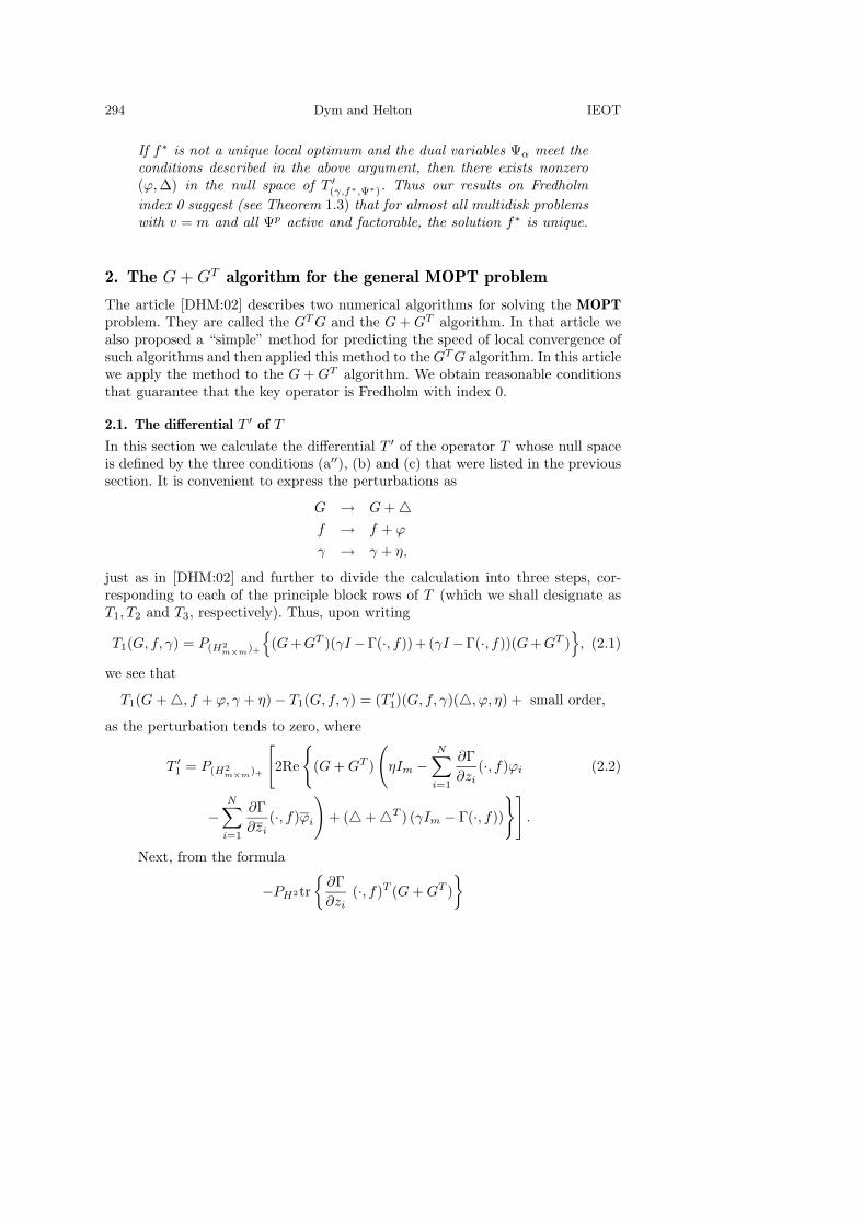
If f∗ is not a unique local optimum and the dual variables Ψα meet theconditions described in the above argument, then there exists nonzero(ϕ,∆) in the null space of T ′
(γ,f∗,Ψ∗). Thus our results on Fredholmindex 0 suggest (see Theorem 1.3) that for almost all multidisk problemswith v = m and all Ψp active and factorable, the solution f∗ is unique.
2. The G + GT algorithm for the general MOPT problem
The article [DHM:02] describes two numerical algorithms for solving the MOPTproblem. They are called the GT G and the G + GT algorithm. In that article wealso proposed a “simple” method for predicting the speed of local convergence ofsuch algorithms and then applied this method to the GT G algorithm. In this articlewe apply the method to the G + GT algorithm. We obtain reasonable conditionsthat guarantee that the key operator is Fredholm with index 0.
2.1. The differential T ′ of T
In this section we calculate the differential T ′ of the operator T whose null spaceis defined by the three conditions (a′′), (b) and (c) that were listed in the previoussection. It is convenient to express the perturbations as
G → G + �f → f + ϕ
γ → γ + η,
just as in [DHM:02] and further to divide the calculation into three steps, cor-responding to each of the principle block rows of T (which we shall designate asT1, T2 and T3, respectively). Thus, upon writing
T1(G, f, γ) = P(H2m×m)+
{(G+GT )(γI −Γ(·, f))+ (γI −Γ(·, f))(G+GT )
}, (2.1)
we see that
T1(G + �, f + ϕ, γ + η) − T1(G, f, γ) = (T ′1)(G, f, γ)(�, ϕ, η) + small order,
as the perturbation tends to zero, where
T ′1 = P(H2
m×m)+
[2Re
{(G + GT )
(ηIm −
N∑i=1
∂Γ∂zi
(·, f)ϕi (2.2)
−N∑
i=1
∂Γ∂zi
(·, f)ϕi
)+ (� + �T ) (γIm − Γ(·, f))
}].
Next, from the formula
−PH2tr{
∂Γ∂zi
(·, f)T (G + GT )}
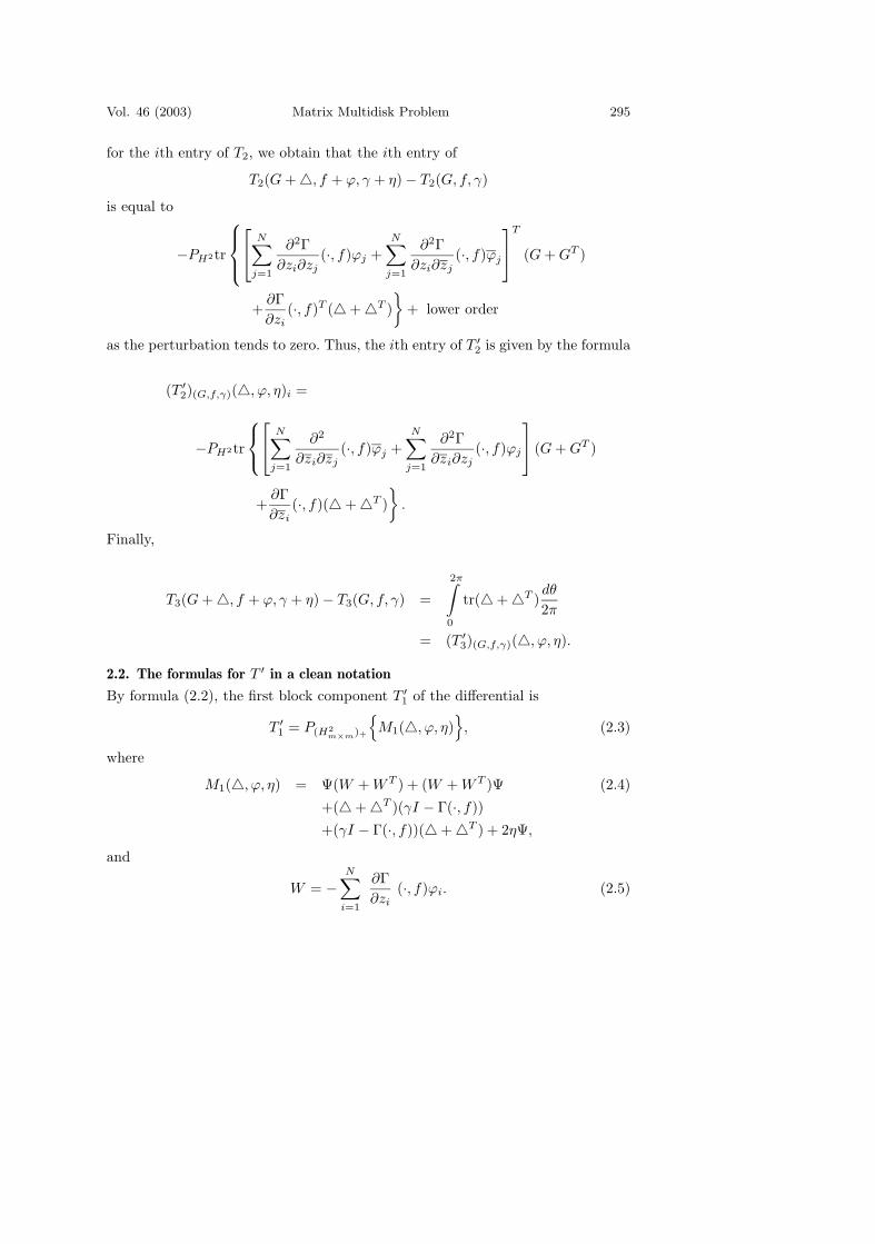
Vol. 46 (2003) Matrix Multidisk Problem 295
for the ith entry of T2, we obtain that the ith entry of
T2(G + �, f + ϕ, γ + η) − T2(G, f, γ)
is equal to
−PH2tr
N∑j=1
∂2Γ∂zi∂zj
(·, f)ϕj +N∑
j=1
∂2Γ∂zi∂zj
(·, f)ϕj
T
(G + GT )
+∂Γ∂zi
(·, f)T (� + �T )}
+ lower order
as the perturbation tends to zero. Thus, the ith entry of T ′2 is given by the formula
(T ′2)(G,f,γ)(�, ϕ, η)i =
−PH2tr
N∑j=1
∂2
∂zi∂zj(·, f)ϕj +
N∑j=1
∂2Γ∂zi∂zj
(·, f)ϕj
(G + GT )
+∂Γ∂zi
(·, f)(� + �T )}
.
Finally,
T3(G + �, f + ϕ, γ + η) − T3(G, f, γ) =
2π∫
0
tr(� + �T )dθ
2π
= (T ′3)(G,f,γ)(�, ϕ, η).
2.2. The formulas for T ′ in a clean notation
By formula (2.2), the first block component T ′1 of the differential is
T ′1 = P(H2
m×m)+
{M1(�, ϕ, η)
}, (2.3)
where
M1(�, ϕ, η) = Ψ(W + WT ) + (W + WT )Ψ (2.4)
+(� + �T )(γI − Γ(·, f))
+(γI − Γ(·, f))(� + �T ) + 2ηΨ,
and
W = −N∑
i=1
∂Γ∂zi
(·, f)ϕi. (2.5)
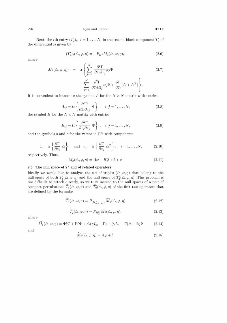
296 Dym and Helton IEOT
Next, the ith entry (T ′2)i, i = 1, . . . , N , in the second block component T ′
2 ofthe differential is given by
(T ′2)i(�, ϕ, η) = −PH2M2(�, ϕ, η)i, (2.6)
where
M2(�, ϕ, η)i = tr
N∑j=1
∂2Γ∂zi∂zj
ϕjΨ (2.7)
+N∑
j=1
∂2Γ∂zi∂zj
ϕjΨ +∂Γ∂zi
(� + �T )
.
It is convenient to introduce the symbol A for the N × N matrix with entries
Aij = tr{
∂2Γ∂zi∂zj
Ψ}
, i, j = 1, . . . , N, (2.8)
the symbol B for the N × N matrix with entries
Bij = tr{
∂2Γ∂zi∂zj
Ψ}
, i, j = 1, . . . , N, (2.9)
and the symbols b and c for the vector in CN with components
bi = tr{
∂Γ∂zi
�}
and ci = tr{
∂Γ∂zi
�T
}, i = 1, . . . , N, (2.10)
respectively. Thus,M2(�, ϕ, η) = Aϕ + Bϕ + b + c. (2.11)
2.3. The null space of T ′ and of related operators
Ideally we would like to analyze the set of triples (�, ϕ, η) that belong to thenull space of both T ′
1(�, ϕ, η) and the null space of T ′2(�, ϕ, η). This problem is
too difficult to attack directly, so we turn instead to the null spaces of a pair ofcompact pertubations T ′
1(�, ϕ, η) and T ′2(�, ϕ, η) of the first two operators that
are defined by the formulas
T ′1(�, ϕ, η) = P(H2
m×m)+M1(�, ϕ, η) (2.12)
T ′2(�, ϕ, η) = PH2
NM2(�, ϕ, η), (2.13)
where
M1(�, ϕ, η) = ΨW + WΨ + �(γIm − Γ) + (γIm − Γ)� + 2ηΨ (2.14)
andM2(�, ϕ, η) = Aϕ + b. (2.15)
Vol. 46 (2003) Matrix Multidisk Problem 297
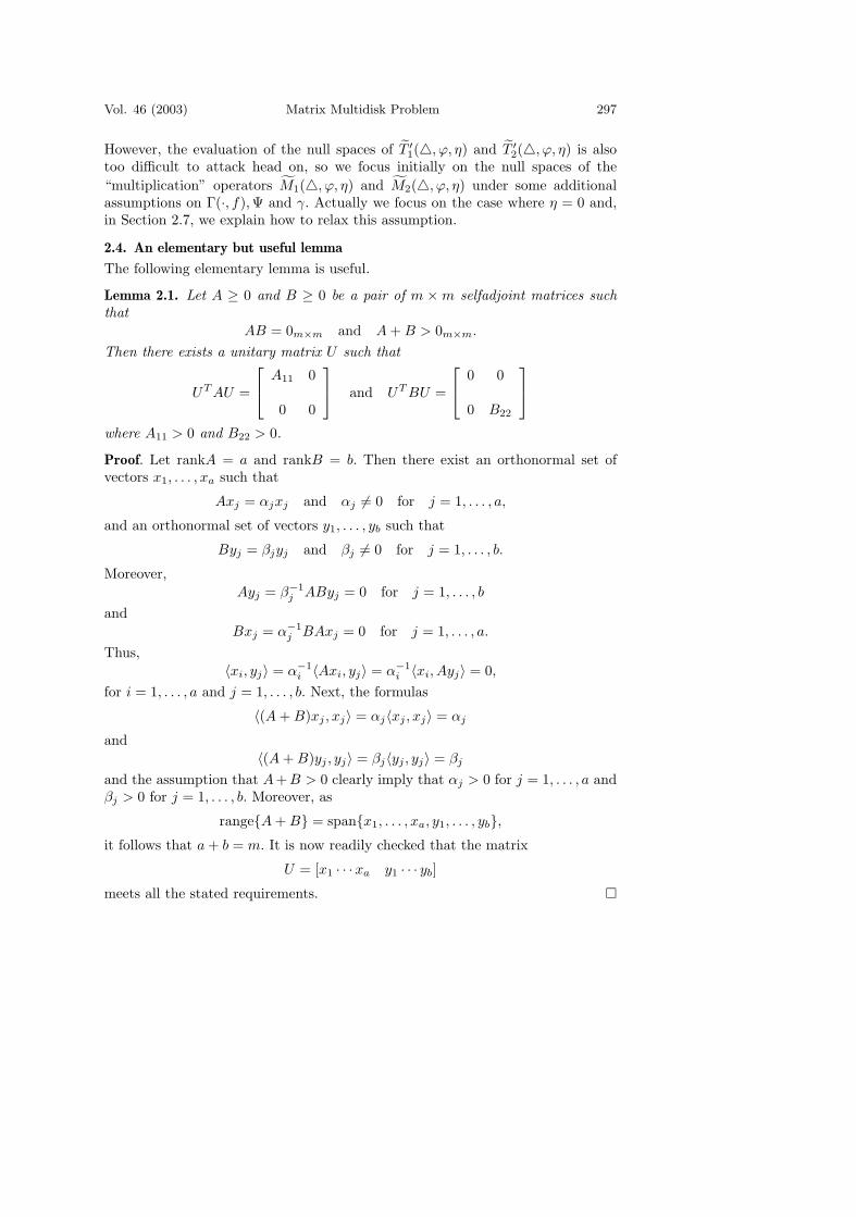
However, the evaluation of the null spaces of T ′1(�, ϕ, η) and T ′
2(�, ϕ, η) is alsotoo difficult to attack head on, so we focus initially on the null spaces of the“multiplication” operators M1(�, ϕ, η) and M2(�, ϕ, η) under some additionalassumptions on Γ(·, f),Ψ and γ. Actually we focus on the case where η = 0 and,in Section 2.7, we explain how to relax this assumption.
2.4. An elementary but useful lemma
The following elementary lemma is useful.
Lemma 2.1. Let A ≥ 0 and B ≥ 0 be a pair of m × m selfadjoint matrices suchthat
AB = 0m×m and A + B > 0m×m.
Then there exists a unitary matrix U such that
UT AU =
A11 0
0 0
and UT BU =
0 0
0 B22
where A11 > 0 and B22 > 0.
Proof. Let rankA = a and rankB = b. Then there exist an orthonormal set ofvectors x1, . . . , xa such that
Axj = αjxj and αj = 0 for j = 1, . . . , a,
and an orthonormal set of vectors y1, . . . , yb such that
Byj = βjyj and βj = 0 for j = 1, . . . , b.
Moreover,Ayj = β−1
j AByj = 0 for j = 1, . . . , b
andBxj = α−1
j BAxj = 0 for j = 1, . . . , a.
Thus,〈xi, yj〉 = α−1
i 〈Axi, yj〉 = α−1i 〈xi, Ayj〉 = 0,
for i = 1, . . . , a and j = 1, . . . , b. Next, the formulas
〈(A + B)xj , xj〉 = αj〈xj , xj〉 = αj
and〈(A + B)yj , yj〉 = βj〈yj , yj〉 = βj
and the assumption that A+B > 0 clearly imply that αj > 0 for j = 1, . . . , a andβj > 0 for j = 1, . . . , b. Moreover, as
range{A + B} = span{x1, . . . , xa, y1, . . . , yb},it follows that a + b = m. It is now readily checked that the matrix
U = [x1 · · ·xa y1 · · · yb]
meets all the stated requirements. �
298 Dym and Helton IEOT
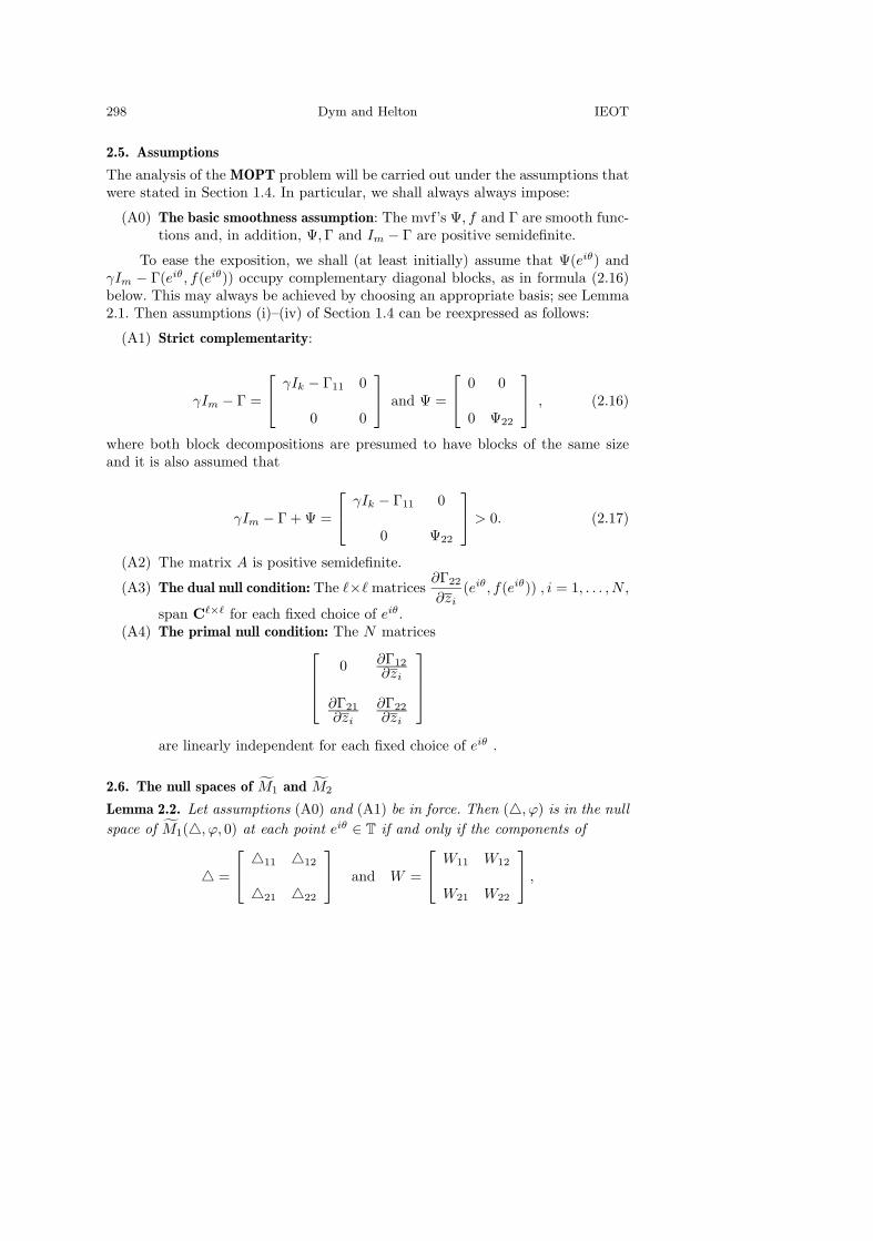
2.5. Assumptions
The analysis of the MOPT problem will be carried out under the assumptions thatwere stated in Section 1.4. In particular, we shall always always impose:
(A0) The basic smoothness assumption: The mvf’s Ψ, f and Γ are smooth func-tions and, in addition, Ψ,Γ and Im − Γ are positive semidefinite.
To ease the exposition, we shall (at least initially) assume that Ψ(eiθ) andγIm − Γ(eiθ, f(eiθ)) occupy complementary diagonal blocks, as in formula (2.16)below. This may always be achieved by choosing an appropriate basis; see Lemma2.1. Then assumptions (i)–(iv) of Section 1.4 can be reexpressed as follows:
(A1) Strict complementarity:
γIm − Γ =
γIk − Γ11 0
0 0
and Ψ =
0 0
0 Ψ22
, (2.16)
where both block decompositions are presumed to have blocks of the same sizeand it is also assumed that
γIm − Γ + Ψ =
γIk − Γ11 0
0 Ψ22
> 0. (2.17)
(A2) The matrix A is positive semidefinite.
(A3) The dual null condition: The × matrices∂Γ22
∂zi(eiθ, f(eiθ)) , i = 1, . . . , N ,
span C�×� for each fixed choice of eiθ.(A4) The primal null condition: The N matrices
0 ∂Γ12∂zi
∂Γ21∂zi
∂Γ22∂zi
are linearly independent for each fixed choice of eiθ .
2.6. The null spaces of M1 and M2
Lemma 2.2. Let assumptions (A0) and (A1) be in force. Then (�, ϕ) is in the nullspace of M1(�, ϕ, 0) at each point eiθ ∈ T if and only if the components of
� =
�11 �12
�21 �22
and W =
W11 W12
W21 W22
,
Vol. 46 (2003) Matrix Multidisk Problem 299
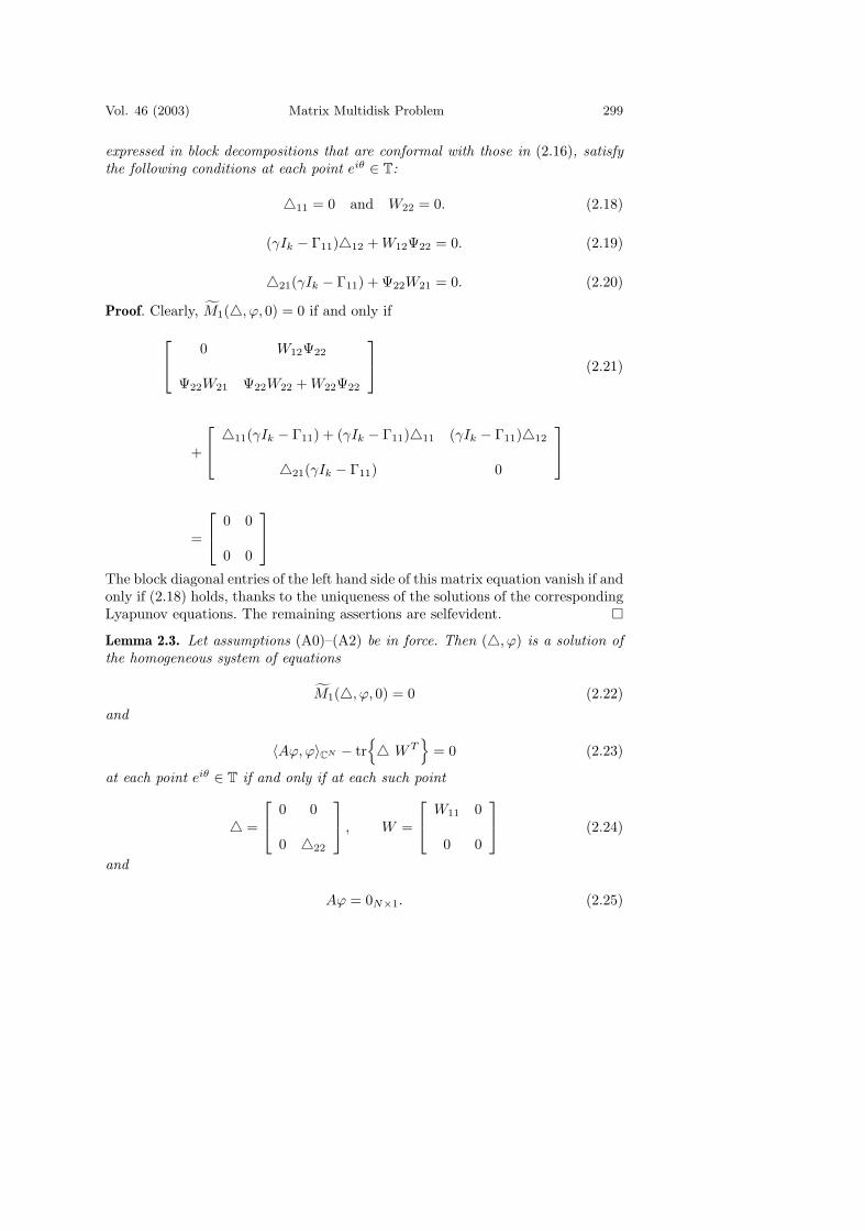
expressed in block decompositions that are conformal with those in (2.16), satisfythe following conditions at each point eiθ ∈ T:
�11 = 0 and W22 = 0. (2.18)
(γIk − Γ11)�12 + W12Ψ22 = 0. (2.19)
�21(γIk − Γ11) + Ψ22W21 = 0. (2.20)
Proof. Clearly, M1(�, ϕ, 0) = 0 if and only if
0 W12Ψ22
Ψ22W21 Ψ22W22 + W22Ψ22
(2.21)
+
�11(γIk − Γ11) + (γIk − Γ11)�11 (γIk − Γ11)�12
�21(γIk − Γ11) 0
=
0 0
0 0
The block diagonal entries of the left hand side of this matrix equation vanish if andonly if (2.18) holds, thanks to the uniqueness of the solutions of the correspondingLyapunov equations. The remaining assertions are selfevident. �Lemma 2.3. Let assumptions (A0)–(A2) be in force. Then (�, ϕ) is a solution ofthe homogeneous system of equations
M1(�, ϕ, 0) = 0 (2.22)and
〈Aϕ,ϕ〉CN − tr{� WT
}= 0 (2.23)
at each point eiθ ∈ T if and only if at each such point
� =
0 0
0 �22
, W =
W11 0
0 0
(2.24)
and
Aϕ = 0N×1. (2.25)
300 Dym and Helton IEOT
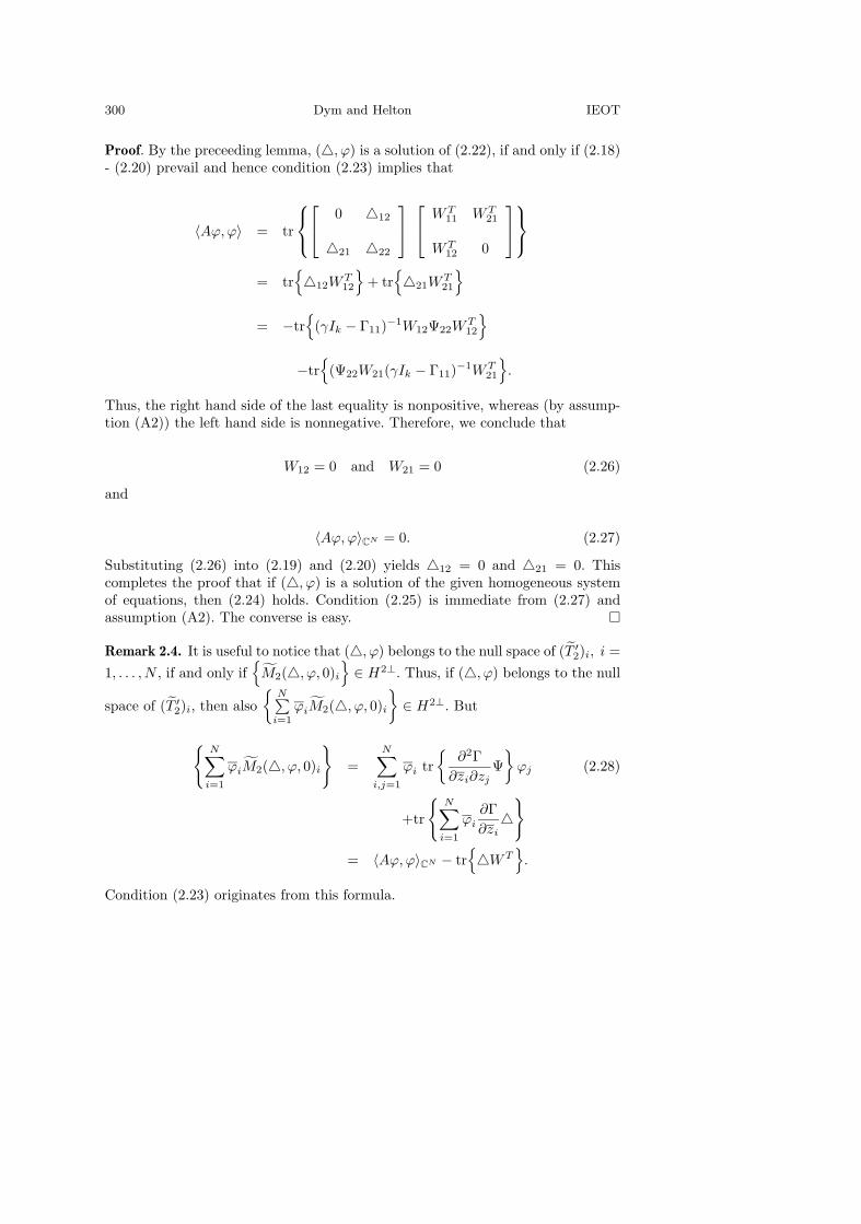
Proof. By the preceeding lemma, (�, ϕ) is a solution of (2.22), if and only if (2.18)- (2.20) prevail and hence condition (2.23) implies that
〈Aϕ,ϕ〉 = tr
0 �12
�21 �22
WT11 WT
21
WT12 0
= tr{�12W
T12
}+ tr
{�21W
T21
}
= −tr{
(γIk − Γ11)−1W12Ψ22WT12
}
−tr{
(Ψ22W21(γIk − Γ11)−1WT21
}.
Thus, the right hand side of the last equality is nonpositive, whereas (by assump-tion (A2)) the left hand side is nonnegative. Therefore, we conclude that
W12 = 0 and W21 = 0 (2.26)
and
〈Aϕ,ϕ〉CN = 0. (2.27)
Substituting (2.26) into (2.19) and (2.20) yields �12 = 0 and �21 = 0. Thiscompletes the proof that if (�, ϕ) is a solution of the given homogeneous systemof equations, then (2.24) holds. Condition (2.25) is immediate from (2.27) andassumption (A2). The converse is easy. �
Remark 2.4. It is useful to notice that (�, ϕ) belongs to the null space of (T ′2)i, i =
1, . . . , N , if and only if{
M2(�, ϕ, 0)i
}∈ H2⊥. Thus, if (�, ϕ) belongs to the null
space of (T ′2)i, then also
{N∑
i=1
ϕiM2(�, ϕ, 0)i
}∈ H2⊥. But
{N∑
i=1
ϕiM2(�, ϕ, 0)i
}=
N∑i,j=1
ϕi tr{
∂2Γ∂zi∂zj
Ψ}
ϕj (2.28)
+tr
{N∑
i=1
ϕi
∂Γ∂zi
�}
= 〈Aϕ,ϕ〉CN − tr{�WT
}.
Condition (2.23) originates from this formula.

Vol. 46 (2003) Matrix Multidisk Problem 301
2.6.1. Formulas for the null spaces of M1 and M2
Lemma 2.5. Let assumptions (A0)–(A2) be in force. Then (�, ϕ) is a solution ofthe homogeneous system of equations
M1(�, ϕ, 0) = 0 and M2(�, ϕ, 0) = 0 (2.29)
at each point eiθ ∈ T if and only if at each point eiθ ∈ T
� =
0 0
0 �22
, W =
W11 0
0 0
, (2.30)
Aϕ = 0 and b = 0. (2.31)
Proof. The necessity of the stated conditions is immediate from the precedinglemma, because the second condition in (2.29) implies (2.23) and (2.25) implies(2.31). The sufficiency is selfevident. �
It remains to translate the condition (2.30) and (2.31) into conditions on �and ϕ, under appropriate assumptions on
∂Γ∂zi
and Ψ. Under the added assumption
(A3), we can strengthen (one direction of) the last theorem:
Lemma 2.6. If assumptions (A0)–(A3) are in force, then (�, ϕ) is a solution ofthe homogeneous system of equations (2.29) at each point eiθ ∈ T if and only if ateach point eiθ
� =
0 0
0 0
, W =
W11 0
0 0
(2.32)
and (2.31) hold.
Proof. Let assumptions (A1)-(A3) be in force. Then the preceding theorem guar-antees that (2.30) and (2.31) hold. Therefore
bi = tr
∂Γ∂zi
0 0
0 �22
= tr{(
∂Γ∂zi
)
22
�22
}= 0.
By assumption (A3) we can find a linear combinationN∑
i=1
ci
(∂Γ∂zi
)22
of the(
∂Γ∂zi
)22
,
i = 1, . . . , N , which is equal to �T22. Therefore, we must have
tr{�22(eiθ)T�22(eiθ)
}= 0,

302 Dym and Helton IEOT
which holds if and only if �22(eiθ) = 0. Thus we see that (A1) - (A3) imply that(2.32) and (2.31) hold. The converse is selfevident.
�
Theorem 2.7. If assumptions (A0)–(A4) are in force, then (�, ϕ) is a solution ofthe homogeneous system of equations (2.29) at each point eiθ ∈ T if and only if� = 0 and ϕ = 0 at each point eiθ ∈ T.
Proof. If (�, ϕ) is a solution of the homogeneous system of equations (2.29) andassumptions (A1)-(A4) are in force, then the preceding theorem guarantees that
∆ = 0 andN∑
i=1
[0 ∂Γ12
∂zi∂Γ21∂zi
∂Γ22∂zi
]ϕi = 0.
Therefore, by assumption (A4), ϕ(eiθ) = 0 for every point eiθ on the unit circle.This completes the proof in one direction. The converse is selfevident. �
2.7. Another variant
Another variant of the last theorem may be obtained by keeping (A0)–(A2) as is,but modifying the conditions (A3) and (A4) as follows:
(A3+) The new dual null condition: The × matrices
I� and∂Γ22
∂zi(eiθ, f(eiθ)) , i = 1, . . . , N,
span C�×� for each fixed choice of eiθ.(A4+) The new primal null condition: The N + 1 matrices
0 0
0 I�
and
0 ∂Γ12∂zi
∂Γ21∂zi
∂Γ22∂zi
are linearly independent for each fixed choice of eiθ .
Theorem 2.8. If assumptions (A0)–(A2), (A3+) and (A4+) are in force, then(�, ϕ, η) is a solution of the homogeneous system of equations
M1(�, ϕ, η) = 0, M2(�, ϕ, η) = 0 and tr{�} = 0 (2.33)
at each point eiθ ∈ T if and only if � = 0, ϕ = 0 and η = 0 at each such point.
Proof. The proof is a simple modification of the proof of Theorem 2.7. It is con-venient to set
W = ηIm + W.
Then, with the help of the extra condition tr{�} = 0, it is readily checked thatLemmas 2.2, 2.3 and 2.5 hold with Mi(�, ϕ, 0) replaced by Mi(�, ϕ, η) and W
replaced by W . Thus, from (A1) and (A2) alone, we see that if (�, ϕ, η) is a solution
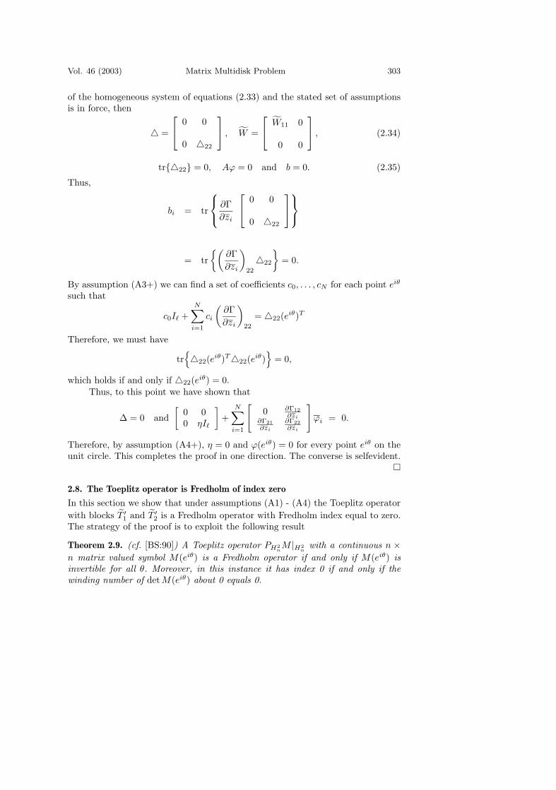
Vol. 46 (2003) Matrix Multidisk Problem 303
of the homogeneous system of equations (2.33) and the stated set of assumptionsis in force, then
� =
0 0
0 �22
, W =
W11 0
0 0
, (2.34)
tr{�22} = 0, Aϕ = 0 and b = 0. (2.35)
Thus,
bi = tr
∂Γ∂zi
0 0
0 �22
= tr{(
∂Γ∂zi
)
22
�22
}= 0.
By assumption (A3+) we can find a set of coefficients c0, . . . , cN for each point eiθ
such that
c0I� +N∑
i=1
ci
(∂Γ∂zi
)
22
= �22(eiθ)T
Therefore, we must have
tr{�22(eiθ)T�22(eiθ)
}= 0,
which holds if and only if �22(eiθ) = 0.Thus, to this point we have shown that
∆ = 0 and[
0 00 ηI�
]+
N∑i=1
[0 ∂Γ12
∂zi∂Γ21∂zi
∂Γ22∂zi
]ϕi = 0.
Therefore, by assumption (A4+), η = 0 and ϕ(eiθ) = 0 for every point eiθ on theunit circle. This completes the proof in one direction. The converse is selfevident.
�
2.8. The Toeplitz operator is Fredholm of index zero
In this section we show that under assumptions (A1) - (A4) the Toeplitz operatorwith blocks T ′
1 and T ′2 is a Fredholm operator with Fredholm index equal to zero.
The strategy of the proof is to exploit the following result
Theorem 2.9. (cf. [BS:90]) A Toeplitz operator PH2nM |H2
nwith a continuous n ×
n matrix valued symbol M(eiθ) is a Fredholm operator if and only if M(eiθ) isinvertible for all θ. Moreover, in this instance it has index 0 if and only if thewinding number of det M(eiθ) about 0 equals 0.
304 Dym and Helton IEOT
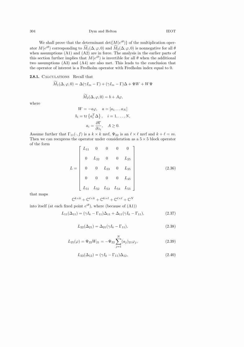
We shall prove that the determinant det{M(eiθ)} of the multiplication oper-ator M(eiθ) corresponding to M1(∆, ϕ, 0) and M2(∆, ϕ, 0) is nonnegative for all θwhen assumptions (A1) and (A2) are in force. The analysis in the earlier parts ofthis section further implies that M(eiθ) is invertible for all θ when the additionaltwo assumptions (A3) and (A4) are also met. This leads to the conclusion thatthe operator of interest is a Fredholm operator with Fredholm index equal to 0.
2.8.1. Calculations Recall that
M1(∆, ϕ, 0) = ∆(γIm − Γ) + (γIm − Γ)∆ + ΨW + WΨ
M2(∆, ϕ, 0) = b + Aϕ,
whereW = −aϕ, a = [a1 . . . aN ]
bi = tr{aT
i ∆}
, i = 1, . . . , N,
ai =∂Γ∂zi
, A ≥ 0.
Assume further that Γ11(·, f) is a k × k mvf, Ψ22 is an × mvf and k + = m.Then we can reexpress the operator under consideration as a 5× 5 block operatorof the form
L =
L11 0 0 0 0
0 L22 0 0 L25
0 0 L33 0 L35
0 0 0 0 L45
L51 L52 L53 L54 L55
(2.36)
that mapsC
k×k + C�×k + C
k� + C�� + C
N
into itself (at each fixed point eiθ), where (because of (A1))
L11(∆11) = (γIk − Γ11)∆11 + ∆11(γIk − Γ11), (2.37)
L22(∆21) = ∆21(γIk − Γ11), (2.38)
L25(ϕ) = Ψ22W21 = −Ψ22
N∑j=1
(aj)21ϕj , (2.39)
L33(∆12) = (γIk − Γ11)∆12, (2.40)
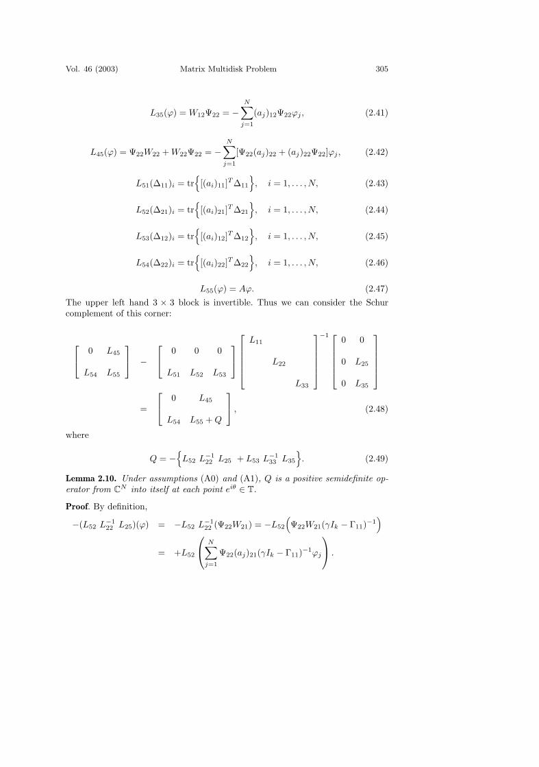
Vol. 46 (2003) Matrix Multidisk Problem 305
L35(ϕ) = W12Ψ22 = −N∑
j=1
(aj)12Ψ22ϕj , (2.41)
L45(ϕ) = Ψ22W22 + W22Ψ22 = −N∑
j=1
[Ψ22(aj)22 + (aj)22Ψ22]ϕj , (2.42)
L51(∆11)i = tr{
[(ai)11]T ∆11
}, i = 1, . . . , N, (2.43)
L52(∆21)i = tr{
[(ai)21]T ∆21
}, i = 1, . . . , N, (2.44)
L53(∆12)i = tr{
[(ai)12]T ∆12
}, i = 1, . . . , N, (2.45)
L54(∆22)i = tr{
[(ai)22]T ∆22
}, i = 1, . . . , N, (2.46)
L55(ϕ) = Aϕ. (2.47)The upper left hand 3 × 3 block is invertible. Thus we can consider the Schurcomplement of this corner:
0 L45
L54 L55
−
0 0 0
L51 L52 L53
L11
L22
L33
−1
0 0
0 L25
0 L35
=
0 L45
L54 L55 + Q
, (2.48)
where
Q = −{
L52 L−122 L25 + L53 L−1
33 L35
}. (2.49)
Lemma 2.10. Under assumptions (A0) and (A1), Q is a positive semidefinite op-erator from C
N into itself at each point eiθ ∈ T.
Proof. By definition,
−(L52 L−122 L25)(ϕ) = −L52 L−1
22 (Ψ22W21) = −L52
(Ψ22W21(γIk − Γ11)−1
)
= +L52
N∑j=1
Ψ22(aj)21(γIk − Γ11)−1ϕj
.
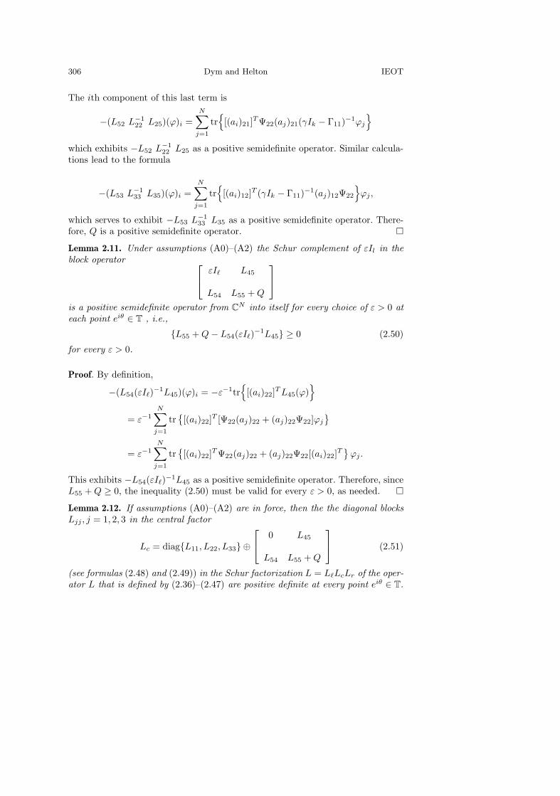
306 Dym and Helton IEOT
The ith component of this last term is
−(L52 L−122 L25)(ϕ)i =
N∑j=1
tr{
[(ai)21]T Ψ22(aj)21(γIk − Γ11)−1ϕj
}
which exhibits −L52 L−122 L25 as a positive semidefinite operator. Similar calcula-
tions lead to the formula
−(L53 L−133 L35)(ϕ)i =
N∑j=1
tr{
[(ai)12]T (γIk − Γ11)−1(aj)12Ψ22
}ϕj ,
which serves to exhibit −L53 L−133 L35 as a positive semidefinite operator. There-
fore, Q is a positive semidefinite operator. �Lemma 2.11. Under assumptions (A0)–(A2) the Schur complement of εIl in theblock operator
εI� L45
L54 L55 + Q
is a positive semidefinite operator from CN into itself for every choice of ε > 0 at
each point eiθ ∈ T , i.e.,
{L55 + Q − L54(εI�)−1L45} ≥ 0 (2.50)
for every ε > 0.
Proof. By definition,
−(L54(εI�)−1L45)(ϕ)i = −ε−1tr{
[(ai)22]T L45(ϕ)}
= ε−1N∑
j=1
tr{[(ai)22]T [Ψ22(aj)22 + (aj)22Ψ22]ϕj
}
= ε−1N∑
j=1
tr{[(ai)22]T Ψ22(aj)22 + (aj)22Ψ22[(ai)22]T
}ϕj .
This exhibits −L54(εI�)−1L45 as a positive semidefinite operator. Therefore, sinceL55 + Q ≥ 0, the inequality (2.50) must be valid for every ε > 0, as needed. �Lemma 2.12. If assumptions (A0)–(A2) are in force, then the the diagonal blocksLjj , j = 1, 2, 3 in the central factor
Lc = diag{L11, L22, L33} ⊕
0 L45
L54 L55 + Q
(2.51)
(see formulas (2.48) and (2.49)) in the Schur factorization L = L�LcLr of the oper-ator L that is defined by (2.36)–(2.47) are positive definite at every point eiθ ∈ T.
Vol. 46 (2003) Matrix Multidisk Problem 307
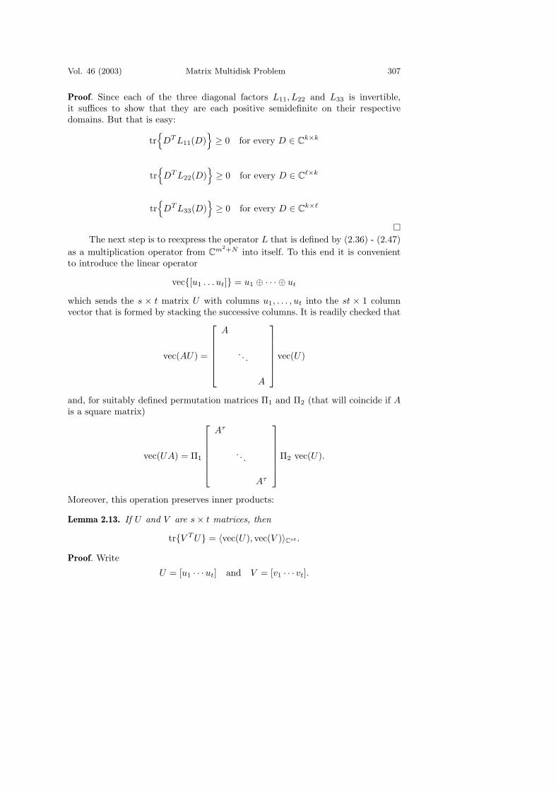
Proof. Since each of the three diagonal factors L11, L22 and L33 is invertible,it suffices to show that they are each positive semidefinite on their respectivedomains. But that is easy:
tr{
DT L11(D)}≥ 0 for every D ∈ C
k×k
tr{
DT L22(D)}≥ 0 for every D ∈ C
�×k
tr{
DT L33(D)}≥ 0 for every D ∈ C
k�
�The next step is to reexpress the operator L that is defined by (2.36) - (2.47)
as a multiplication operator from Cm2+N into itself. To this end it is convenient
to introduce the linear operator
vec{[u1 . . . ut]} = u1 ⊕ · · · ⊕ ut
which sends the s × t matrix U with columns u1, . . . , ut into the st × 1 columnvector that is formed by stacking the successive columns. It is readily checked that
vec(AU) =
A
. . .
A
vec(U)
and, for suitably defined permutation matrices Π1 and Π2 (that will coincide if Ais a square matrix)
vec(UA) = Π1
Aτ
. . .
Aτ
Π2 vec(U).
Moreover, this operation preserves inner products:
Lemma 2.13. If U and V are s × t matrices, then
tr{V T U} = 〈vec(U), vec(V )〉Cst .
Proof. Write
U = [u1 · · ·ut] and V = [v1 · · · vt].

308 Dym and Helton IEOT
Then,
tr{V T U} = tr{UV T } = tr
{t∑
j=1
ujvTj
}=
t∑j=1
tr{ujv
Tj
}=
t∑j=1
vTj uj
= 〈vec(U), vec(V )〉.�
Theorem 2.14. Let L denote the (m2 + N)× (m2 + N) matrix corresponding to Lthat acts on
vec(∆11) ⊕ vec(∆21) ⊕ vec(∆12) ⊕ vec(∆22) ⊕ ϕ
and assume that (A0)–(A2) are in force. Then
detL ≥ 0
at each point eiθ ∈ T.
Proof. The first step is to factor L as L = L�LcLr, where
Ll =
I 0 0 0 0
0 I 0 0 0
0 0 I 0 0
0 0 0 I 0
L51L−111 L52L
−122 L53L
−133 0 I
, Lr =
I 0 0 0 0
0 I 0 0 L−122 L25
0 0 I 0 L−133 L35
0 0 0 I 0
0 0 0 0 I
(2.52)and Lc is given by (2.51). All these operators map
Ck×k + C
�×k + Ck×� + C
�� + CN
into itself (at each fixed point eiθ). Correspondingly,
L = L�LcLr
anddetL = detLc,
since L� is lower triangular with one’s on the diagonal and Lr is upper triangularwith ones on the diagonal. Moreover, detLc ≥ 0 by Lemmas 2.11 and 2.12. �Theorem 2.15. Let assumptions (A0)–(A4) be in force. Then the operator
T ′1
T ′2
T ′3
:
∆
ϕ
η
→
T ′1(∆, ϕ, η)
T ′2(∆, ϕ, η)
T ′3(∆, ϕ, η)
is a Fredholm operator of index zero.
Vol. 46 (2003) Matrix Multidisk Problem 309
Proof. The operator of interest with the T ′3 row set to 0 and with η = 0 has the same
Fredholm index as the original operator and is equivalent to PH2m2+N
L|Hm2+N .By our earlier analysis, (A1)–(A4) ⇒ L is invertible,whereas, by Theorem 2.14,detL ≥ 0. Now invoke the general result Theorem 2.9 to finish. �
3. G + GT Applied to the Nehari Problem
The performance function for the Nehari problem is
Γ(·, Z) = (K − Z)(K − Z)T , (3.1)
whereK = K(eiθ)
is a continuous m × m mvf on the unit circle and
Z = [zij ], i, j = 1, . . . , m.
Consequently,
∂Γ∂zij
= −Eij(K − Z)T ,∂Γ∂zst
= −(K − Z)Ets (3.2)
and∂2Γ
∂zst∂zij= EijEts. (3.3)
Thus, upon writingϕ = (ϕij), i, j = 1, . . . , m,
we see that
W = −m∑
i,j=1
∂Γ∂zij
ϕij = ϕ(K − f)T (3.4)
and that the st entry of the “vectors” Aϕ and b are given by
[Aϕ]st =m∑
i,j=1
tr{
∂2Γ∂zst∂zij
Ψ}
ϕij = tr{
ϕEtsΨ}
= (Ψϕ)st (3.5)
and
bst = tr{
∂Γ∂zst
�}
= −tr{
(K − f)Ets�}
= −(�(K − f)
)st
. (3.6)
Consequently,
M1(�, ϕ, 0) = Ψϕ(K − f)T + ϕ(K − f)T Ψ + �(γIm − Γ) + (γIm − Γ)� (3.7)
andM2(�, ϕ, 0) = Ψϕ −�(K − f). (3.8)
310 Dym and Helton IEOT
Lemma 3.1. In the setting of the Nehari problem, subject to assumption (A0), themvf A with entries
Ast,ij = tr{
∂2Γ∂zst∂zij
Ψ}
is positive semidefinite at every point eiθ ∈ T.
Proof. In view of formula (3.5), it is readily seen that
m∑s,t=1
m∑i,j=1
cst(Ast,ij)cij = tr
{m∑
s,t=1
m∑i,j=1
cstEijEtsΨcij
}= tr
{CCT Ψ
}
= tr{
CT ΨC}
,
where C is the m × m matrix with ij entry equal to cij . �
3.1. The null space of the symbol of the Toeplitz operator T ′
We begin with a characterization of the null space of the modified multiplicationoperators M1(�, ϕ, 0) and M2(�, ϕ, 0).
Recall that in the setting of the Nehari problem,
Aϕ = Ψϕ, b = −�(K − f) (3.9)
and
M2(�, ϕ, 0) = Aϕ + b = Ψϕ −�(K − f). (3.10)
Moreover, since W is given by formula (3.4) and A is positive semidefinite, byLemma 3.1, it is readily seen that the following result is in force.
Theorem 3.2. In the setting of the Nehari problem, let assumptions (A0)–(A1) bein force and let γ > 0. Then (�, ϕ) is in the null space of both M1(�, ϕ, 0) andM2(�, ϕ, 0) at every point eiθ ∈ T if and only if
� =
0 0
0 �22
, W =
W11 0
0 0
, (3.11)
Ψϕ = 0 and �(K − f) = 0 (3.12)
at every point eiθ ∈ T. (Thus, if (K − f) or even (K − f)22 is invertible, then�22 = 0 also.)
Proof. This is an immediate consequence of the formulas in (3.9) and Lemma 2.5,since in the setting of the Nehari problem the assumption (A2) is automaticallysatisfied. �
Vol. 46 (2003) Matrix Multidisk Problem 311
3.2. The primal and dual null conditions
In this subsection we examine the implications of assumptions (A3) and (A4) inthe setting of the Nehari problem. Let
P2 = P2(eiθ) = Ψ†(eiθ)Ψ(eiθ)
andP1 = P1(eiθ) = Im − P2(eiθ).
It is often convenient, though not essential, to think of these two complementaryorthogonal projectors as
P1 =[
Ik 00 0
]and P2 =
[0 00 I�
];
its really the “fielder’s choice,” since it makes no difference to the present analysis.In any event, since P2Ψ = Ψ, we have
{K(eiθ) − f(eiθ)}CΨ(eiθ) = 0 ⇐⇒ {K(eiθ) − f(eiθ)}CP2(eiθ) = 0
for any m × m matrix C. Then, as
∂Γ22
∂zij(·, f) = −P2{(K − f)Eji}P2,
condition (A3) is the same as to say that
(A3′) {P2(K − f)CP2 : C ∈ Cm×m} = {P2DP2 : D ∈ C
m×m}.By taking orthogonal complements in the vector space C
m×m endowed withthe trace norm, the condition (A3) for the Nehari problem is easily seen to beequivalent to the condition
(A3′′) (K − f)T P2DP2 = 0 ⇒ P2DP2 = 0.
Lemma 3.3. If (A0) and (A1) are in force for the Nehari problem and γ > 0, thencondition (A3) is automatically met.
Proof. Let(K − f)T P2DP2 = 0
for some matrix D ∈ Cm×m. Then clearly
P2(K − f)(K − f)T P2DP2 = 0
also. But condition (A1) implies that
γP2 = P2(K − f)(K − f)T P2
and hence thatγP2DP2 = 0.
�
312 Dym and Helton IEOT
We turn next to the primal null condition. In terms of the projectors P1 andP2, it states that for each choice of eiθ the set of m2 matrices
(K − f)EjiP2 + P2K − f)EjiP1
(that are obtained by letting i, j = 1, . . . , m) are linearly independent. This is thesame as to say that
(A4′) (K − f)CP2 + P2(K − f)CP1 = 0m×m ⇐⇒ C = 0m×m.
Since P1P2 = P2P1 = 0, the conditions on the left hand side of (A4′) decouple toyield the two conditions:
(A4′′)(K − f)CP2 = 0 =⇒ CP2 = 0
P2(K − f)CP1 = 0 =⇒ CP1 = 0.
If (K−f) is invertible, then the first of these last two conditions will be met.However, the second of these two conditions cannot hold, unless P1 = 0. Thus, thepreceding discussion leads to the following conclusions:
Theorem 3.4. Let (A0) and (A1) be in force for the Nehari problem. Then:1. (A2) is automatically in force.2. If γ > 0, then (A3) is automatically in force.3. If m > 1, then (A4) is never met.
3.3. A detour on factorization
In this section we show how our optimality conditions yield the classical Hankeloperator optimality conditions for the Nehari problem.
Lemma 3.5. Let γ∗, f∗andΨ∗ meet the optimality conditions (a), (b) and (c) thatare given in Section 1.2 and suppose that Ψ∗ admits a factorization of the formΨ∗ = GT G, where G is a continuous k × m mvf in H2
k×m that is outer. Then, inthe setting of the Nehari problem, (a) and (b) are equivalent to
{γ∗ − Γ(eiθ, f∗(eiθ))
}GT (eiθ) = 0 (3.13)
and(K(eiθ) − f∗(eiθ))T GT (eiθ)G(eiθ) ∈ eiθH2
m×m. (3.14)
Proof. The equivalence of (a) and (3.13) is selfevident, since
γ∗ − Γ(eiθ, f∗(eiθ)) = {γ∗ − Γ(eiθ, f∗(eiθ))}T .
To obtain (3.14), invoke formula (3.2) to reexpress (b) as
0 = PH2 tr {(K(eiθ) − f∗(eiθ))EjiGT (eiθ)G(eiθ)}
= PH2 tr {EjiGT (eiθ)G(eiθ)(K(eiθ) − f∗(eiθ))}
= PH2{[GT (eiθ)G(eiθ)(K(eiθ) − f∗(eiθ)]ij}for i, j = 1, . . . , m. Thus (b) is clearly equivalent to
GT (eiθ)G(eiθ)(K(eiθ) − f∗(eiθ)) = e−iθF (eiθ)T
Vol. 46 (2003) Matrix Multidisk Problem 313
for some F ∈ H2m×m. But this in turn implies that
(K(eiθ) − f∗(eiθ))T GT (eiθ)G(eiθ) = eiθF (eiθ),
which is equivalent to (3.14). �
Lemma 3.6. In the setting of the previous lemma, condition (3.14) holds if andonly if
(K(eiθ) − f∗(eiθ))T G(eiθ)T ∈ eiθH2m×k (3.15)
or, in other notation with χ(eiθ) = eiθ, if and only if
(K − f∗)T GT ∈ χH2m×k
Proof. Assume first that
(K − f∗)T GT G ∈ χH2m×m
and let P be an m × k matrix polynomial in eiθ. Then
(K − f∗)T GT GP ∈ χH2m×k.
Thus the Fourier coefficients
{(K − f∗)T GT GP}∧(k)
vanish for k ≤ 0. Now, since G is outer, we can choose a sequence of m× k matrixpolynomials Pn, n = 1, 2, . . . , such that
2π∫
0
tr{(GPn − Ik)T (GPn − Ik)
} → 0.
Then the Fourier coefficients{(K − f∗)T GT (Ik − GPn)
}∧(k) → 0 as n → ∞.
Consequently, {(K − f∗)T GT
}∧(k) = 0 for k ≤ 0.
�This leads to the following Hankel formulation of the optimality conditions:
Theorem 3.7. Let u be any vector in Ck. Then the setting of Lemma 3.5
γ∗GT u = PχH2⊥m
KPχH2m
KT GT u.
Proof. By (3.13) and Lemma 3.6,
γ∗GT u = (K − f∗)(K − f∗)T GT u
= PχH2⊥m
(K − f∗)(PχH2⊥m
+ PχH2m
)(K − f∗)T GT u
= PχH2⊥m
(K − f∗)PχH2m
(K − f∗)T GT u.
But this is readily seen to reduce to the stated formula, since f∗ does not con-tribute. �

314 Dym and Helton IEOT
Remark 3.8. The condition in the last theorem can also be expressed as
γ∗χ−1GT u = PH2⊥m
KPH2m
KT χ−1GT u.
4. The G + GT Algorithm for The Multidisk Problem
In this section we shall study the G + GT algorithm for the multidisk problem.
4.1. The setting
We shall assume thatΓ = diag{Γ1, . . . ,Γv},
whereΓp(·, Z) = (Kp − Z)(Kp − Z)T
for p = 1, . . . , v, the Kp are continuous m × m mvf’s on T and
Z = [zij ], i, j = 1, . . . , m.
We shall also assume that
G = diag{G1, . . . , Gv},where Gp is a continuous m × m mvf on T that belongs to H∞
m×m and that
Ψp(eiθ) = Gp(eiθ) + Gp(eiθ)T
is positive semidefinite on T.
4.2. The operators T and T ′
The operator T1 for this setting is equal to
diag{T 11 (G1, f, γ), . . . , T v
1 (Gv, f, γ)},where the block components are obtained from (2.1). Hence, the differential T ′
1
may be evaluated one block at a time. Since the calculations for each block are thesame as the calculations for the Nehari problem, we invoke formulas (2.3), (2.4)and (3.4) to obtain
(T p1 )′ = P(H2
m×m)+
[2Re
{Ψp(η + W p + W pT
) + δp(γI − Γp)}]
, (4.1)
whereW p = ϕ(Kp − f)T
andδp = ∆p + ∆pT
,
for p = 1, . . . , v.
Vol. 46 (2003) Matrix Multidisk Problem 315
Next, we exploit the fact that the trace of a block diagonal operator
A = diag{A1, . . . , Av}is the sum of the traces of each of its blocks, i.e.,
tr{A} =v∑
p=1
tr{Ap}
to calculate T ′2 for this setting. The result is
T ′2(∆, ϕ, η) = PH2
m×m
{(v∑
p=1
Ψp
)ϕ −
v∑p=1
(∆pT
+ ∆p)(Kp − f)
}. (4.2)
Finally
T ′3(∆, ϕ, η) =
v∑p=1
12π
∫ 2π
0
tr{∆pT
+ ∆p}dθ. (4.3)
4.3. The symbol of the Toeplitz operators T ′
Let
Mp1 (∆, ϕ, η) = Ψp(ηp + W p + W pT
) (4.4)
+(ηp + W p + W pT
)Ψp
+δp(γpI − Γp) + (γpI − Γp)δp
and
M2(∆, ϕ, η) =
(v∑
p=1
Ψp
)ϕ −
v∑p=1
δp(Kp − f), (4.5)
whereδp = ∆p + ∆pT
.
These are the multiplication operators which appear in the definitions of the com-ponents T ′
1 and T ′2 of the differential, respectively. Allowing compact perturbations
of the differential permits us to work with a Toeplitz operator T ′ wherein all termsinvolving ϕT and ∆pT
are discarded.In particular, the symbol of T ′ is
Mp1 (∆, ϕ, 0) = ΨpW p + W pΨp + ∆p(γIm − Γp) + (γIm − Γp)∆p (4.6)
for p = 1, . . . , v and
M2(∆, ϕ, 0) =
(v∑
p=1
Ψp
)ϕ −
v∑p=1
∆p(Kp − f). (4.7)
316 Dym and Helton IEOT
4.4. Strict complementarity
In the present multidisk setting, the assumption of strict complementarity meansthat
(γIm − Γp)Ψp = 0 (4.8)and
(γIm − Γp) + Ψp > 0 (4.9)for p = 1, . . . , m at every point eiθ ∈ T.
In view of Lemma 2.1, we see that assumption of strict complementarily inthe multidisk case is equivalent to assuming the existence of v unitary matricesU1, . . . , Uv such that
UpT
(γpI − Γp)Up =
γpI − Γp11 0
0 0
(4.10)
UpT
ΨpUp =
0 0
0 Ψp22
, (4.11)
where the two block decompositions are the same size and the nonzero entry ineach is positive definite.
4.5. The null space of the modified multiplication operators
In this subsection we calculate the null space of the modified multiplication oper-ators under the assumption of strict complementarity. Then, upon writing
UpT
W pUp =
W p11 W p
12
W p21 W p
22
and UpT
∆pUp =
∆p11 ∆p
12
∆p21 ∆p
22
and invoking exactly the same arguments that were used to analyze the Nehariproblem, we see that the condition
Mp1 (∆, ϕ, 0) = 0
holds if and only if
∆p11 = 0 , W p
22 = 0 (4.12)
(γI − Γp11)∆
p12 + W p
12Ψp22 = 0 (4.13)
and
∆p21(γI − Γp
11) + Ψp22W
p21 = 0 (4.14)
Vol. 46 (2003) Matrix Multidisk Problem 317
for p = 1, . . . , v. Next, the condition
M2(∆, ϕ, 0) = 0
implies that
(v∑
p=1
Ψp
)ϕϕT =
v∑p=1
∆pW pT
=v∑
p=1
Up
0 ∆p12
∆p21 ∆p
22
W pT
11 W pT
21
W pT
12 0
UpT
where Up, p = 1, . . . , v, are unitary. Therefore, the trace of the right hand side ofthe last equality is equal to
v∑p=1
tr{
∆p12W
pT
12 + ∆p21W
pT
21
}
= −v∑
p=1
tr{
(γI − Γp11)
−1W p12Ψ
p22W
pT
12
}−
v∑p=1
tr{
Ψp22W
p21(γI − Γp
11)−1W pT
21
}
≤ 0,
since each of the summands is nonnegative. On the other hand, since
tr
{v∑
p=1
ΨpϕϕT
}= tr
{ϕT
(v∑
p=1
Ψp
)ϕ
}≥ 0,
it follows that each of the summands referred to earlier must vanish. In otherwords, we must have,
W p12 = 0 and W p
21 = 0 (4.15)
for p = 1, . . . , v and
ϕT
(v∑
p=1
Ψp
)ϕ = 0. (4.16)
Therefore, since Ψp ≥ 0, we also have
Ψpϕ = 0 (4.17)
and, by formulas (4.13) and (4.14),
∆p12 = 0 and ∆p
21 = 0. (4.18)
Thus we have obtained “half” of the following conclusion:
318 Dym and Helton IEOT
Theorem 4.1. Let assumptions (A0) and (A1) be in force and let γ > 0. Then(∆p, ϕp), p = 1, . . . , v, is a solution of the homogeneous system of equations
Mp1 (∆, ϕ, 0) = 0, p = 1, . . . , v, (4.19)
M2(∆, ϕ, 0) = 0, (4.20)
at every point eiθ ∈ T if and only if the following sets of conditions are met ateach such point:
∆p =
0 0
0 ∆p22
, W p =
W p11 0
0 0
, p = 1, . . . , v, (4.21)
(Ψp)ϕ = 0 andv∑
p=1
∆p(Kp − f) = 0. (4.22)
Proof. The proof that (4.19) and (4.20) imply (4.21) and (4.22) was given beforethe statement of the theorem. The converse is selfevident. �
4.6. The primal and dual null conditions
In this subsection we examine assumptions (A3) and (A4) restricted to the settingof the multidisk problem.
It is convenient to set
P1 = diag(P
(1)1 , . . . , P
(v)1
)
and
P2 = diag(P
(1)2 , . . . , P
(v)2
),
where
P(p)1 = the orthogonal projection onto the range of γIm −Γp(eiθ, f(eiθ)), p =
1, . . . , v,
and
P(p)2 = the orthogonal projection onto the range of Ψp(eiθ), p = 1, . . . , v.
The strict complementarity assumption means P(p)1 and P
(p)2 are complemen-
tary orthogonal projectors on Cm for p = 1, . . . , v. Thus, in this case, the numbers
kp = rankP(p)1 and p = rankP
(p)2
sum to m:kp + p = m.
Vol. 46 (2003) Matrix Multidisk Problem 319
In view of formula (3.2), adapted to the multidisk setting, it is readily seen thatcondition (A3) for the multidisk problem states that
(A3′)
{diag
(P
(1)2 (K1 − f)CP
(1)2 , . . . , P
(v)2 (Kv − f)CP
(v)2
): C ∈ C
m×m}
={
diag(P
(1)2 DP
(1)2 , . . . , P
(v)2 DP
(v)2
): D ∈ C
m×m}
The last condition can be reformulated, much as in the Nehari case, by looking atorthogonal complements with respect to the trace norm. That is to say, (A3′) isequivalent to the statement that the zero matrix is the only matrix of the form.
diag(P
(1)2 DP
(1)2 , . . . , P
(v)2 DP
(v)2
)
that is orthogonal to the set of matrices on the left of (A3′) with respect to thetrace norm. Thus, (A3) is also equivalent to the condition
(A3′′)v∑
p=1
(Kp − f)T P(p)2 DP
(p)2 = 0 =⇒ P
(p)2 DP
(p)2 = 0 for p = 1, . . . , v.
Next, it is readily checked that in the multidisk setting, condition (A4) statesthat the m2 matrices
diag((K1 − f)Eij , . . . , (Kv − f)Eij
) · P2
+P2 · diag((K1 − f)Eij , . . . , (Kv − f)Eij
) · P1
are linearly independent. But this is the same as to say that
(A4′) (Kp − f)CP(p)2 + P
(p)2 (Kp − f)CP
(p)1
= 0 for p = 1, . . . , v =⇒ C = Om×m.
SinceP
(p)2 P
(p)1 = P
(p)1 P
(p)2 = 0 for p = 1, . . . , v,
the conditions on the left of (A4′) can be decoupled to yield:(A4′′)(Kp − f)CP
(p)2 = 0 and P
(p)2 (Kp − f)C = 0 for p = 1, . . . , v =⇒ C = Om×m.
Thus, the situation in the multidisk case can be summarized in terms of the or-thogonal projectors P
(p)1 = P
(p)1 (eiθ) and P
(p)2 = P
(p)2 (eiθ) as follows:
Theorem 4.2. In the multidisk setting, assume that (A0) is in force and that everypoint eiθ ∈ T
ψp(eiθ) ≥ 0 γIm − Γp(eiθ, f(eiθ)
) ≥ 0 for p = 1, . . . , v (4.23)
and the following conditions are met:
(A1′′) P(p)1 + P
(p)2 = Im and P
(p)1 P
(p)2 = 0, for p = 1, . . . , v.
(A3′′)
N∑p=1
{Kp(eiθ) − f(eiθ)}T P(p)2 DP
(p)2 = 0 ⇒ P
(p)2 DP
(p)2 = 0
for p = 1, . . . , v and every D ∈ Cm×m.
320 Dym and Helton IEOT
(A4′′) {Kp(eiθ) − f(eiθ)}C P(p)2 = 0 and P
(p)2 (Kp(eiθ) − f(eiθ)C = 0
for p = 1, . . . , v and C ∈ Cm×m ⇒ C = 0.
Then the operator T ′ defined in Section 4.2 is a Fredholm operator of index zero.
This theorem can be reformulated in terms of the positive semidefinite mvf’sΨp(eiθ) and γIm − Γp(eiθ, f(eiθ)) as follows:
Theorem 4.3. In the multidisk setting, assume that (A0) and (4.23) are in forceand that the following conditions are met for every point eiθ:(A1′′) Ψp(eiθ)(γIm−Γp(eiθ, f(eiθ)))=0 and Ψp(eiθ)+(γIm−Γp(eiθ, f(eiθ))>0,
for p=1, . . . , v.
(A3′′)
v∑p=1
{Kp(eiθ) − f(eiθ)}T Ψp(eiθ)DΨp(eiθ)=0 =⇒ Ψp(eiθ)DΨp(eiθ)=0
for p = 1, . . . , v and every D ∈ Cm×m.
(A4′′) {Kp(eiθ) − f(eiθ)}C Ψp(eiθ) = 0 and Ψp(eiθ)(Kp(eiθ) − f(eiθ)C = 0for p = 1, . . . , v and C ∈ C
m×m =⇒ C = 0.
Then the operator T ′ defined in Section 4.2 is a Fredholm operator of index zero.
Lemma 4.4. If the row vectors in the spaces P(p)2 (Kp−f), p = 1, . . . , m, span C
m×1
at every point eiθ ∈ T, then (A4) holds.
Proof. Let the conditions on the left hand side of (A4′′) be in force. Then clearly
P(p)2 (Kp − f)C = 0 for p = 1, . . . , v.
But this clearly forces C = 0 under the conditions of the lemma. �
5. A matrix norm minimization problem
In this section, we consider the problem of calculating
γ∗ = minx1,...,xn∈R
‖(C −N∑
j=1
xjAj)2‖, (5.1)
where C and Aj , j = 1, . . . , N , are real symmetric m × m matrices. This is anMOPT problem with
Γ(eiθ, z) = (C −N∑
j=1
xjAj)2 (5.2)
andzj = xj + iyj , j = 1, . . . , N.
Note that Γ is independent of eiθ.To analyze this problem, let
Z = γIm − Γ(eiθ, z) (5.3)
= γIm − (C −N∑
j=1
xjAj)2.
Vol. 46 (2003) Matrix Multidisk Problem 321
Then, since
2∂Γ∂zj
=∂Γ∂xj
= − ∂Z
∂xj= −(C −
N∑i=1
xiAi)Aj − Aj(C −N∑
i=1
xiAi),
our previous analysis indicates that at optimum, there exists an m×m matrix Y(that is playing the role of Ψ(eiθ)), such that the following three conditions (thatcorrespond to (a), (b) and (c) of Section 1.2) are met:
(α) Y Z = 0.(β) tr{BjY } = 0, j = 1, . . . , N.(γ) tr{Y } − 1 = 0,
where
Bj =∂Z
∂xj= (C −
N∑i=1
xiAi)Aj + Aj(C −N∑
i=1
xiAi).
Moreover,(δ) Z ≥ 0 and Y ≥ 0.
Therefore, as noted earlier, the condition (α) is equivalent to the condition(α′) Y Z + ZY = 0.
Thus, upon replacing (α) by (α′), we end up studying the null space of the operator
T :
Yx1
...xN
γ
∈
Sm×m
⊕R
N
⊕R
→
Y Z + ZYtr{B1Y }
...tr{BNY }tr{Y } − 1
∈
Sm×m
⊕R
N
⊕R
,
where Sm×m denotes the vector space of real symmetric m × m matrices. Next,upon setting x = (x1, . . . , xN ) and ε = (ε, . . . , εN ), consideration of
T (Y + ∆Y ;x + ε; γ + η) − T (Y ;x; γ)
leads readily to the formulas
T ′(Y ; x; γ)(∆Y ; ε; η) =
(∆Y )Z + Z(∆Y ) + Y (∆Z) + (∆Z)Y
tr{−N∑
i=1
εi(AiA1 + A1Ai)Y + B1(∆Y )}...
tr{−∑εi(AiAN + ANAi)Y + BN (∆Y )}
tr{∆Y }
(5.4)
∆Z = ηIm +N∑
j=1
εjBj (5.5)
for the differential (alias the Jacobian) of the map T .
322 Dym and Helton IEOT
5.1. The conditions (B1)–(B4)
To avoid overburdening the notation, we shall label the conditions that correspondto (A1)–(A4) in this new setting by (B1)–(B4), respectively. In view of Lemma2.1, there is no loss of generality in writing the strict complementarity conditionas:
(B1) Z =[
Z11 00 0
]and
[0 00 Y22
]with blocks Z11 > 0 of size k × k,
Y22 > 0 of size × , where k + = m.
Moreover, since
4∂2Γ
∂zi∂zj= AiAj + AjAi,
and Y ≥ 0, the matrix defined by formula (2.8) is automatically positive semidef-inite, i.e., condition (A2) is automatically met.
Next, since we cannot discard compact operators in the present finite dimen-sional setting, we need to modify the dual null condition and primal null conditiona bit: In addition to
− ∂Γ∂zj
=∂Z
∂xj= Bj , j = 1, . . . , N,
we shall make use of
B0 =∂Z
∂γ= Im.
The modified dual null condition and primal null condition reduce to:
(B3) The matrices (Bj)22, j = 0, . . . , N , span S��.(B4) The matrices
[0 (Bj)12(Bj)21 (Bj)22
], j = 0, . . . , N,
are linearly independent in Cm×m.
A simple dimension count leads readily to the conclusion that in order for theconditions (B3) and (B4) to both hold, the number N must satisfy the inequalities
( + 1)2
≤ N + 1 ≤ m(m + 1)2
− k(k + 1)2
,
or equivalently, since m = + k, that
( + 1)2
≤ N + 1 ≤ (m + k + 1)2
. (5.6)
Lemma 5.1. Let (B1) be in force and, in the setting of this section, let (∆Y ; ε; η)belong to the null space of T ′ (i.e., let the right hand side of formula (5.4) vanish).Then
∆Z =[
(∆Z)11 00 0
]and ∆Y =
[0 00 (∆Y )22
]. (5.7)
Vol. 46 (2003) Matrix Multidisk Problem 323
Proof. It is readily seen (just as in the proof of Lemma 2.2) that
(∆Y )Z + Z(∆Y ) + Y (∆Z) + (∆Z)Y = 0 (5.8)
holds if and only if(∆Y )11 = 0, (∆Z)22 = 0 (5.9)
Z11(∆Y )12 + (∆Z)12Y22 = 0 and (∆Y )21Z11 + Y22(∆Z)21 = 0. (5.10)
However, since ∆Y ∈ Sm×m and ∆Z ∈ Sm×m the last two conditions (on the offdiagonal terms of ∆Y and ∆Z) are equivalent. The conditions (5.9) and (5.10)imply that
tr{(∆Z)(∆Y )} = tr{[
(∆Z)11 (∆Z)12(∆Z)21 0
] [0 (∆Y )12
(∆Y )21 (∆Y )22
]}
= 2tr{(∆Z)12(∆Y )21}= −2tr{Z11(∆Y )12(Y22)−1(∆Y )21}= −2tr{[(Y22)−1/2(∆Y )21(Z11)1/2]T (Y22)−1/2(∆Y )21(Z11)1/2}≤ 0.
On the other hand, upon invoking formulas (5.4) and (5.5), we obtain
tr{(∆Z)(∆Y )} = tr{η(∆Y )} +N∑
j=1
εjtr{Bj(∆Y )}
=N∑
j=1
εjtr{Bj(∆Y )}
= tr
N∑i=1,j=1
εi(AiAj + AjAi)εjY
= 2tr
{(N∑
i=1
εiAi
)Y
(N∑
i=1
εiAi
)}≥ 0.
Therefore, tr{(∆Z)(∆Y )} = 0, which in turn implies that (∆Y )21 = 0, (∆Y )12 = 0and hence, by formula (5.10), we also have that (∆Z)12 = 0 and (∆Z)21 = 0. Thiscompletes the proof. �
Lemma 5.2. Let (B1) and (B3) be in force and, in the setting of this section, let(∆Y ; ε; η) belong to the null space of T ′ (i.e., let the right hand side of formula(5.4) vanish). Then
∆Z =[
(∆Z)11 00 0
]and ∆Y = 0. (5.11)
324 Dym and Helton IEOT
Proof. Let (B1) be in force and let (∆Y ; ε; η) be in the null space of T ′. Then,
0 = tr{−N∑
i=1
εi(AiAj + AjAi)Y + Bj(∆Y )}.
Therefore, upon multiplying through by εj and summing over j, we obtain theformula
0 = tr
−
N∑i,j=1
εi(AiAj + AjAi)εjY +N∑
j=1
Bjεj(∆Y )
.
But this is the same as to say
2tr
{(N∑
i=1
εiAi
)Y
(N∑
i=1
εiAi
)}= tr
{N∑
i=1
Biεi(∆Y )
}
= tr{(∆Z)(∆Y ) − ηIm(∆Y )}= 0.
Thus, as the left hand side of the last equality is positive semidefinite, it followsthat
0 =N∑
i=1
εiAiY =N∑
i=1
Y εiAi
and hence that
0 = tr{Bj(∆Y )} = tr{(Bj)22(∆Y )22}.This equality holds for j = 0 as well as for j = 1, . . . , N. Moreover, by (B3), wecan find a set of real numbers c0, . . . , cN such that
N∑j=0
cj(Bj)22 = {(∆Y )22}T = (∆Y )22.
Therefore,
tr[{(∆Y )22}T (∆Y )22
]= 0.
But this clearly implies that (∆Y )22 = 0 as claimed. �
Theorem 5.3. Let (B1), (B3) and (B4) be in force. Then, in the setting of thissection, the following statements are equivalent:
1. (∆Y ; ε; η) is in the null space of T ′ (i.e., the right hand side of formula(5.4) vanishes).
2. ∆Y = 0 and ∆Z = 0.3. ∆Y = 0, η = 0 and ε = 0.
In other words, T ′ is invertible.
Vol. 46 (2003) Matrix Multidisk Problem 325
Proof. Let (B1), (B3) and (B4) be in force and let (∆Y ; ε; η) belong to the nullspace of T ′. Then, in view of the last lemma, ∆Y = 0 and
∆Z =[
(∆Z)11 00 0
]= ηIm +
N∑j=1
εjBj .
However, the last formula can be reexpressed as:
(∆Z)11 = ηIk +N∑
j=1
εj(Bj)11 (5.12)
and[
0 00 0
]= η
[0 00 I�
]+
N∑j=1
εj
[0 (B12)j
(B21)j (B22)j
]. (5.13)
Assumption (B4) applied to the formula (5.13) forces η = 0 and εj = 0, j =1, . . . , N , and hence, by formula (5.12), also implies that (∆Z)11 = 0. This com-pletes the proof that (1) ⇒ (2) and (1) ⇒ (3). Much the same argument serves toprove that (2) ⇒ (3). The proof that (3) ⇒ 1 is selfevident. �
6. A matrix eigenvalue minimization problem
In this section we consider the problem of calculating
γ∗ = minx1,...,xN∈R
γ subject to γIm ≥ C −N∑
j=1
xjAj , (6.1)
where C and Aj , j = 1, . . . , N , are real symmetric matrices. This resembles an(MOPT) problem with
Γ(x) = C −N∑
j=1
xjAj ,
but the fact that Γ is not positive semidefinite valued violates the set up of theMOPT problem. Fortunately a generalization of the MOPT theory applies, seeChapters 19, 20 of [HM:98] (especially Theorem 19.1.4), and gives optimality con-ditions for this problem which closely resemble what we have to come expect.However, for this simple setup, it is possible to establish the needed conditionsdirectly, as we shall begin to show in the next paragraph. We mention that the op-timization problem (6.1) is similar to, but not the same as, the problem consideredin the article [AHO:98]. The conclusions are also similar.
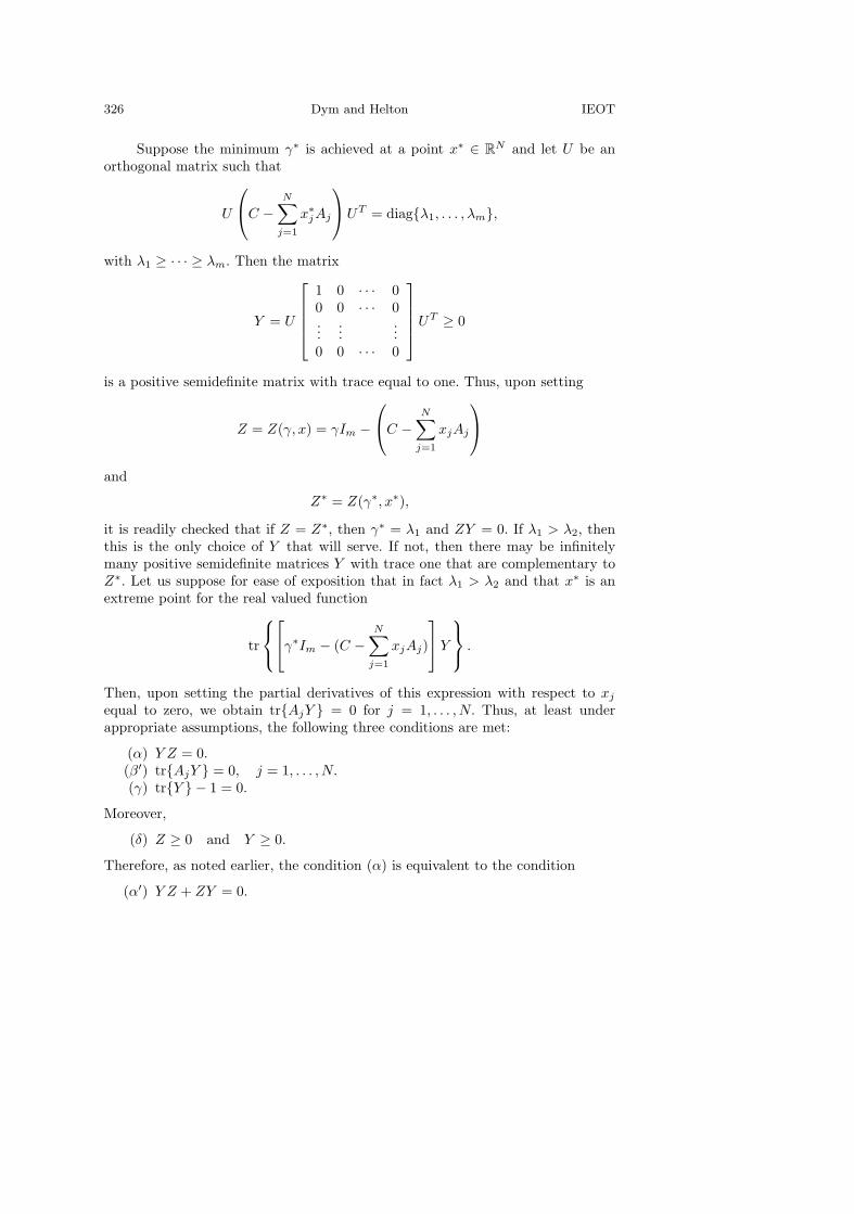
326 Dym and Helton IEOT
Suppose the minimum γ∗ is achieved at a point x∗ ∈ RN and let U be an
orthogonal matrix such that
U
C −
N∑j=1
x∗jAj
UT = diag{λ1, . . . , λm},
with λ1 ≥ · · · ≥ λm. Then the matrix
Y = U
1 0 · · · 00 0 · · · 0...
......
0 0 · · · 0
UT ≥ 0
is a positive semidefinite matrix with trace equal to one. Thus, upon setting
Z = Z(γ, x) = γIm −C −
N∑j=1
xjAj
and
Z∗ = Z(γ∗, x∗),
it is readily checked that if Z = Z∗, then γ∗ = λ1 and ZY = 0. If λ1 > λ2, thenthis is the only choice of Y that will serve. If not, then there may be infinitelymany positive semidefinite matrices Y with trace one that are complementary toZ∗. Let us suppose for ease of exposition that in fact λ1 > λ2 and that x∗ is anextreme point for the real valued function
tr
γ∗Im − (C −
N∑j=1
xjAj)
Y
.
Then, upon setting the partial derivatives of this expression with respect to xj
equal to zero, we obtain tr{AjY } = 0 for j = 1, . . . , N. Thus, at least underappropriate assumptions, the following three conditions are met:
(α) Y Z = 0.(β′) tr{AjY } = 0, j = 1, . . . , N.(γ) tr{Y } − 1 = 0.
Moreover,
(δ) Z ≥ 0 and Y ≥ 0.
Therefore, as noted earlier, the condition (α) is equivalent to the condition
(α′) Y Z + ZY = 0.
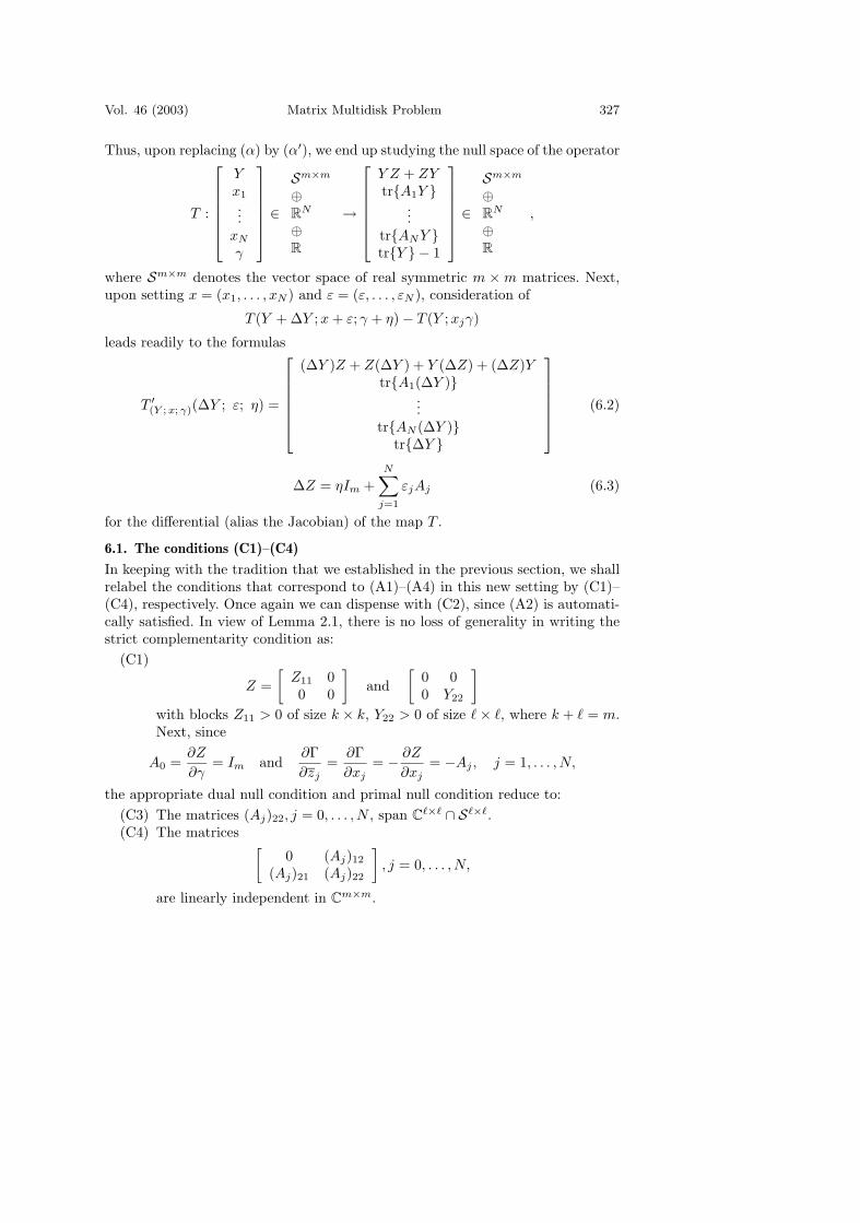
Vol. 46 (2003) Matrix Multidisk Problem 327
Thus, upon replacing (α) by (α′), we end up studying the null space of the operator
T :
Yx1
...xN
γ
∈
Sm×m
⊕R
N
⊕R
→
Y Z + ZYtr{A1Y }
...tr{ANY }tr{Y } − 1
∈
Sm×m
⊕R
N
⊕R
,
where Sm×m denotes the vector space of real symmetric m × m matrices. Next,upon setting x = (x1, . . . , xN ) and ε = (ε, . . . , εN ), consideration of
T (Y + ∆Y ;x + ε; γ + η) − T (Y ;xjγ)
leads readily to the formulas
T ′(Y ; x; γ)(∆Y ; ε; η) =
(∆Y )Z + Z(∆Y ) + Y (∆Z) + (∆Z)Ytr{A1(∆Y )}
...tr{AN (∆Y )}
tr{∆Y }
(6.2)
∆Z = ηIm +N∑
j=1
εjAj (6.3)
for the differential (alias the Jacobian) of the map T .
6.1. The conditions (C1)–(C4)
In keeping with the tradition that we established in the previous section, we shallrelabel the conditions that correspond to (A1)–(A4) in this new setting by (C1)–(C4), respectively. Once again we can dispense with (C2), since (A2) is automati-cally satisfied. In view of Lemma 2.1, there is no loss of generality in writing thestrict complementarity condition as:
(C1)
Z =[
Z11 00 0
]and
[0 00 Y22
]
with blocks Z11 > 0 of size k × k, Y22 > 0 of size × , where k + = m.Next, since
A0 =∂Z
∂γ= Im and
∂Γ∂zj
=∂Γ∂xj
= − ∂Z
∂xj= −Aj , j = 1, . . . , N,
the appropriate dual null condition and primal null condition reduce to:(C3) The matrices (Aj)22, j = 0, . . . , N , span C
�×� ∩ S�×�.(C4) The matrices [
0 (Aj)12(Aj)21 (Aj)22
], j = 0, . . . , N,
are linearly independent in Cm×m.
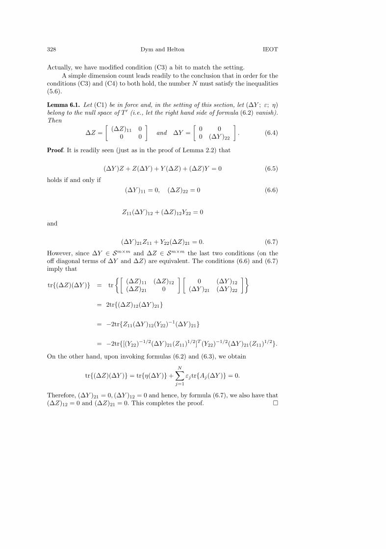
328 Dym and Helton IEOT
Actually, we have modified condition (C3) a bit to match the setting.A simple dimension count leads readily to the conclusion that in order for the
conditions (C3) and (C4) to both hold, the number N must satisfy the inequalities(5.6).
Lemma 6.1. Let (C1) be in force and, in the setting of this section, let (∆Y ; ε; η)belong to the null space of T ′ (i.e., let the right hand side of formula (6.2) vanish).Then
∆Z =[
(∆Z)11 00 0
]and ∆Y =
[0 00 (∆Y )22
]. (6.4)
Proof. It is readily seen (just as in the proof of Lemma 2.2) that
(∆Y )Z + Z(∆Y ) + Y (∆Z) + (∆Z)Y = 0 (6.5)
holds if and only if
(∆Y )11 = 0, (∆Z)22 = 0 (6.6)
Z11(∆Y )12 + (∆Z)12Y22 = 0
and
(∆Y )21Z11 + Y22(∆Z)21 = 0. (6.7)
However, since ∆Y ∈ Sm×m and ∆Z ∈ Sm×m the last two conditions (on theoff diagonal terms of ∆Y and ∆Z) are equivalent. The conditions (6.6) and (6.7)imply that
tr{(∆Z)(∆Y )} = tr{[
(∆Z)11 (∆Z)12(∆Z)21 0
] [0 (∆Y )12
(∆Y )21 (∆Y )22
]}
= 2tr{(∆Z)12(∆Y )21}
= −2tr{Z11(∆Y )12(Y22)−1(∆Y )21}
= −2tr{[(Y22)−1/2(∆Y )21(Z11)1/2]T (Y22)−1/2(∆Y )21(Z11)1/2}.On the other hand, upon invoking formulas (6.2) and (6.3), we obtain
tr{(∆Z)(∆Y )} = tr{η(∆Y )} +N∑
j=1
εjtr{Aj(∆Y )} = 0.
Therefore, (∆Y )21 = 0, (∆Y )12 = 0 and hence, by formula (6.7), we also have that(∆Z)12 = 0 and (∆Z)21 = 0. This completes the proof. �
Vol. 46 (2003) Matrix Multidisk Problem 329
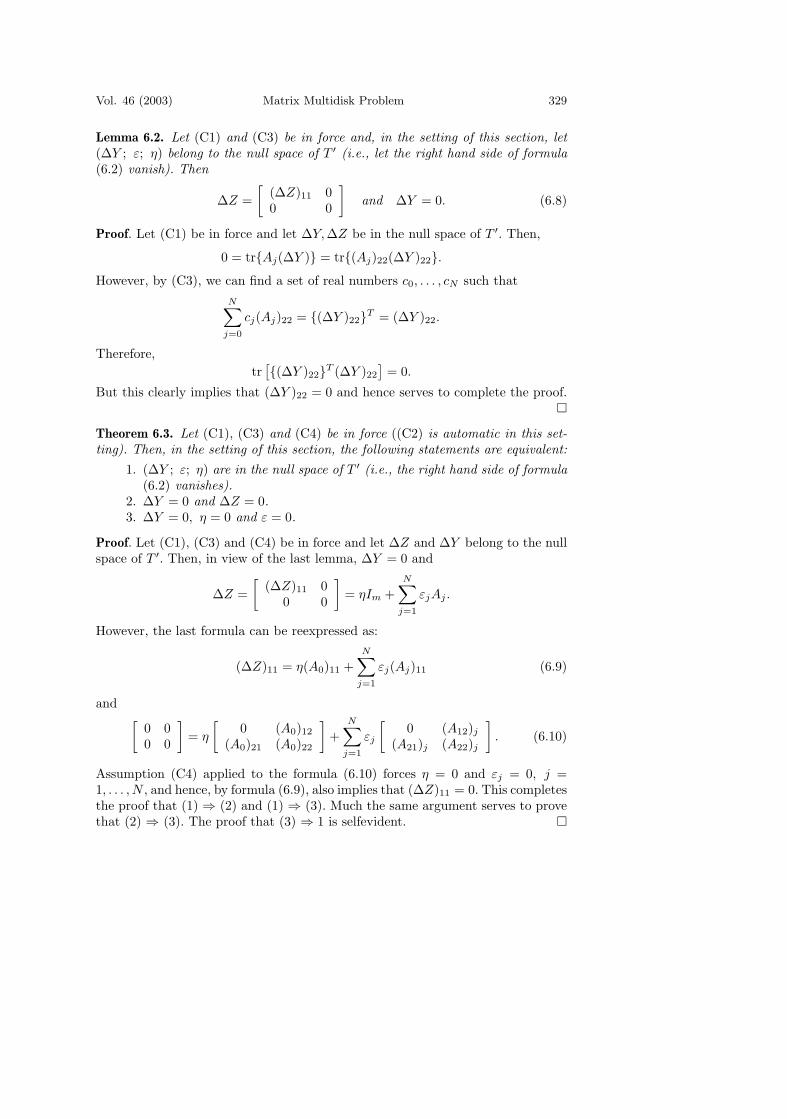
Lemma 6.2. Let (C1) and (C3) be in force and, in the setting of this section, let(∆Y ; ε; η) belong to the null space of T ′ (i.e., let the right hand side of formula(6.2) vanish). Then
∆Z =[
(∆Z)11 00 0
]and ∆Y = 0. (6.8)
Proof. Let (C1) be in force and let ∆Y,∆Z be in the null space of T ′. Then,
0 = tr{Aj(∆Y )} = tr{(Aj)22(∆Y )22}.However, by (C3), we can find a set of real numbers c0, . . . , cN such that
N∑j=0
cj(Aj)22 = {(∆Y )22}T = (∆Y )22.
Therefore,tr[{(∆Y )22}T (∆Y )22
]= 0.
But this clearly implies that (∆Y )22 = 0 and hence serves to complete the proof.�
Theorem 6.3. Let (C1), (C3) and (C4) be in force ((C2) is automatic in this set-ting). Then, in the setting of this section, the following statements are equivalent:
1. (∆Y ; ε; η) are in the null space of T ′ (i.e., the right hand side of formula(6.2) vanishes).
2. ∆Y = 0 and ∆Z = 0.3. ∆Y = 0, η = 0 and ε = 0.
Proof. Let (C1), (C3) and (C4) be in force and let ∆Z and ∆Y belong to the nullspace of T ′. Then, in view of the last lemma, ∆Y = 0 and
∆Z =[
(∆Z)11 00 0
]= ηIm +
N∑j=1
εjAj .
However, the last formula can be reexpressed as:
(∆Z)11 = η(A0)11 +N∑
j=1
εj(Aj)11 (6.9)
and[
0 00 0
]= η
[0 (A0)12
(A0)21 (A0)22
]+
N∑j=1
εj
[0 (A12)j
(A21)j (A22)j
]. (6.10)
Assumption (C4) applied to the formula (6.10) forces η = 0 and εj = 0, j =1, . . . , N , and hence, by formula (6.9), also implies that (∆Z)11 = 0. This completesthe proof that (1) ⇒ (2) and (1) ⇒ (3). Much the same argument serves to provethat (2) ⇒ (3). The proof that (3) ⇒ 1 is selfevident. �
330 Dym and Helton IEOT
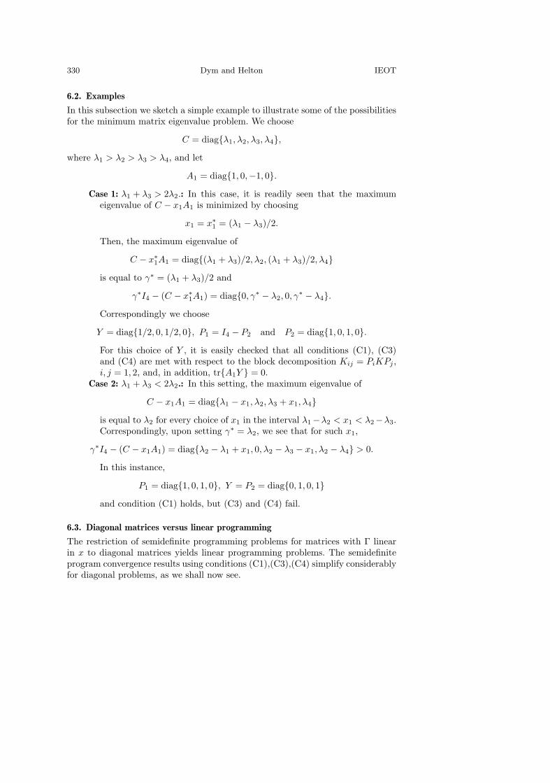
6.2. Examples
In this subsection we sketch a simple example to illustrate some of the possibilitiesfor the minimum matrix eigenvalue problem. We choose
C = diag{λ1, λ2, λ3, λ4},where λ1 > λ2 > λ3 > λ4, and let
A1 = diag{1, 0,−1, 0}.Case 1: λ1 + λ3 > 2λ2.: In this case, it is readily seen that the maximum
eigenvalue of C − x1A1 is minimized by choosing
x1 = x∗1 = (λ1 − λ3)/2.
Then, the maximum eigenvalue of
C − x∗1A1 = diag{(λ1 + λ3)/2, λ2, (λ1 + λ3)/2, λ4}
is equal to γ∗ = (λ1 + λ3)/2 and
γ∗I4 − (C − x∗1A1) = diag{0, γ∗ − λ2, 0, γ∗ − λ4}.
Correspondingly we choose
Y = diag{1/2, 0, 1/2, 0}, P1 = I4 − P2 and P2 = diag{1, 0, 1, 0}.For this choice of Y , it is easily checked that all conditions (C1), (C3)and (C4) are met with respect to the block decomposition Kij = PiKPj ,i, j = 1, 2, and, in addition, tr{A1Y } = 0.
Case 2: λ1 + λ3 < 2λ2.: In this setting, the maximum eigenvalue of
C − x1A1 = diag{λ1 − x1, λ2, λ3 + x1, λ4}is equal to λ2 for every choice of x1 in the interval λ1−λ2 < x1 < λ2−λ3.Correspondingly, upon setting γ∗ = λ2, we see that for such x1,
γ∗I4 − (C − x1A1) = diag{λ2 − λ1 + x1, 0, λ2 − λ3 − x1, λ2 − λ4} > 0.
In this instance,
P1 = diag{1, 0, 1, 0}, Y = P2 = diag{0, 1, 0, 1}and condition (C1) holds, but (C3) and (C4) fail.
6.3. Diagonal matrices versus linear programming
The restriction of semidefinite programming problems for matrices with Γ linearin x to diagonal matrices yields linear programming problems. The semidefiniteprogram convergence results using conditions (C1),(C3),(C4) simplify considerablyfor diagonal problems, as we shall now see.
Vol. 46 (2003) Matrix Multidisk Problem 331
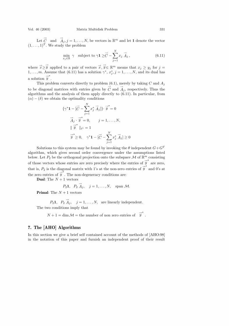
Let→C and
→Aj , j = 1, . . . , N, be vectors in R
m and let 1 denote the vector(1, . . . , 1)T . We study the problem
minxj∈R
γ subject to γ1 ≥→C −
N∑j=1
xj
→Aj , (6.11)
where→x≥→
y applied to a pair of vectors→x,
→y∈ R
m means that xj ≥ yj for j =1, . . . , m. Assume that (6.11) has a solution γ∗, x∗
j , j = 1, . . . , N , and its dual has
a solution→y∗.
This problem converts directly to problem (6.1), merely by taking C and Aj
to be diagonal matrices with entries given by→C and
→Aj , respectively. Thus the
algorithms and the analysis of them apply directly to (6.11). In particular, from(α) − (δ) we obtain the optimality conditions
{γ∗1 − [→C −
N∑j=1
x∗j
→Aj ]}·
→y∗= 0
→Aj · →
y∗= 0, j = 1, . . . , N,
‖ →y∗‖�1 = 1
→y∗≥ 0, γ∗1 − [
→C −
N∑j=1
x∗j
→Aj ] ≥ 0
Solutions to this system may be found by invoking the θ independent G+GT
algorithm, which gives second order convergence under the assumptions listedbelow. Let P2 be the orthogonal projection onto the subspace M of R
m consistingof those vectors whose entries are zero precisely where the entries of
→y∗
are zero,that is, P2 is the diagonal matrix with 1’s at the non-zero entries of
→y∗
and 0’s atthe zero entries of
→y∗. The non-degeneracy conditions are:
Dual: The N + 1 vectors
P21, P2
→Aj , j = 1, . . . , N, span M.
Primal: The N + 1 vectors
P21, P2
→Aj , j = 1, . . . , N, are linearly independent.
The two conditions imply that
N + 1 = dimM = the number of non zero entries of→y∗
.
7. The [AHO] Algorithms
In this section we give a brief self contained account of the methods of [AHO:98]in the notation of this paper and furnish an independent proof of their result
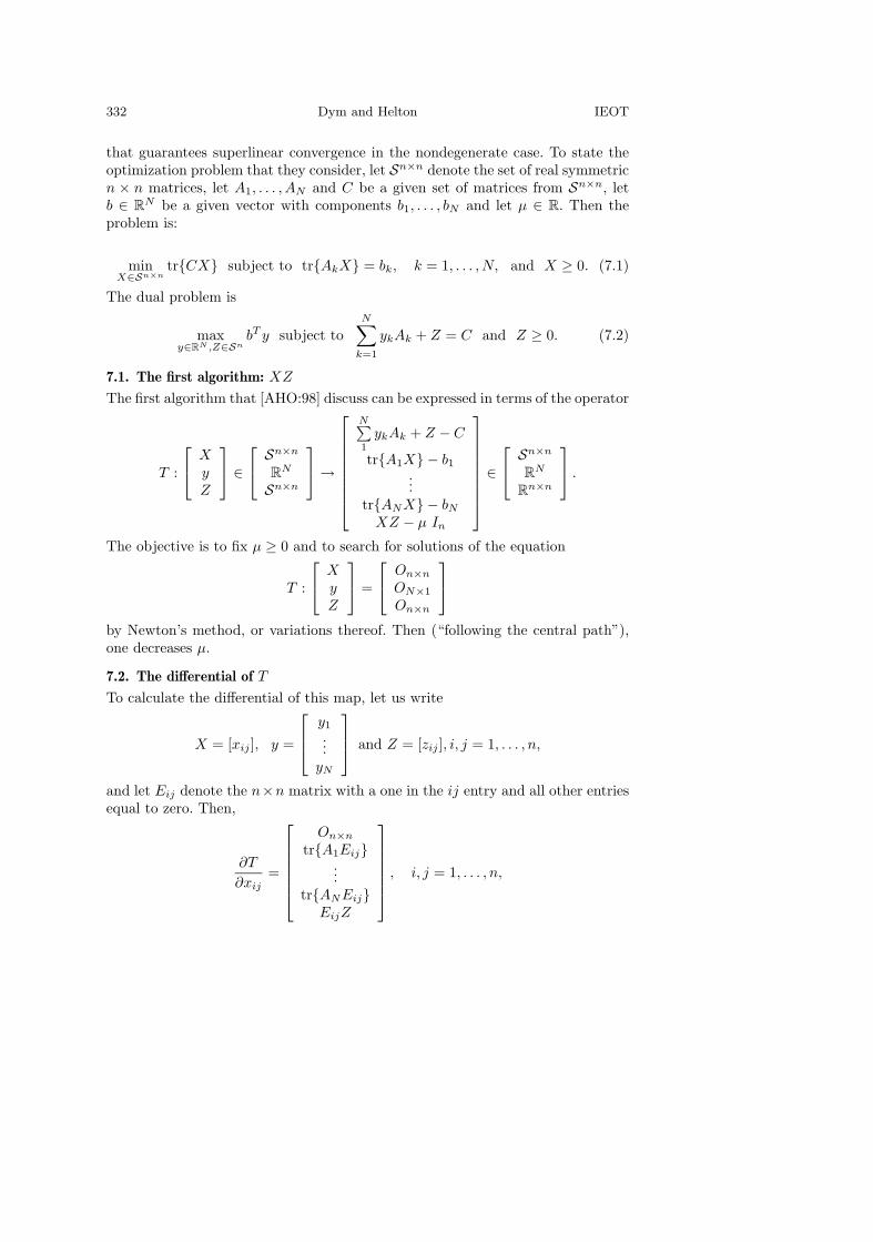
332 Dym and Helton IEOT
that guarantees superlinear convergence in the nondegenerate case. To state theoptimization problem that they consider, let Sn×n denote the set of real symmetricn × n matrices, let A1, . . . , AN and C be a given set of matrices from Sn×n, letb ∈ R
N be a given vector with components b1, . . . , bN and let µ ∈ R. Then theproblem is:
minX∈Sn×n
tr{CX} subject to tr{AkX} = bk, k = 1, . . . , N, and X ≥ 0. (7.1)
The dual problem is
maxy∈RN ,Z∈Sn
bT y subject toN∑
k=1
ykAk + Z = C and Z ≥ 0. (7.2)
7.1. The first algorithm: XZ
The first algorithm that [AHO:98] discuss can be expressed in terms of the operator
T :
XyZ
∈
Sn×n
RN
Sn×n
→
N∑1
ykAk + Z − C
tr{A1X} − b1
...tr{ANX} − bN
XZ − µ In
∈
Sn×n
RN
Rn×n
.
The objective is to fix µ ≥ 0 and to search for solutions of the equation
T :
XyZ
=
On×n
ON×1
On×n
by Newton’s method, or variations thereof. Then (“following the central path”),one decreases µ.
7.2. The differential of T
To calculate the differential of this map, let us write
X = [xij ], y =
y1
...yN
and Z = [zij ], i, j = 1, . . . , n,
and let Eij denote the n×n matrix with a one in the ij entry and all other entriesequal to zero. Then,
∂T
∂xij=
On×n
tr{A1Eij}...
tr{ANEij}EijZ
, i, j = 1, . . . , n,
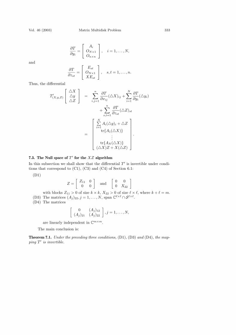
Vol. 46 (2003) Matrix Multidisk Problem 333
∂T
∂yi=
Ai
ON×1
On×n
, i = 1, . . . , N,
and
∂T
∂zst=
Est
ON×1
XEst
, s, t = 1, . . . , n.
Thus, the differential
T ′(X,y,Z)
�X�y�Z
=
n∑i,j=1
∂T
∂xij(�X)ij +
N∑i=1
∂T
∂yi(�yi)
+n∑
s,t=1
∂T
∂zst(�Z)st
=
N∑i=1
Ai(�y)i + �Z
tr{A1(�X)}...
tr{AN (�X)}(�X)Z + X(�Z)
.
7.3. The Null space of T ′ for the XZ algorithm
In this subsection we shall show that the differential T ′ is invertible under condi-tions that correspond to (C1), (C3) and (C4) of Section 6.1:
(D1)
Z =[
Z11 00 0
]and
[0 00 X22
]
with blocks Z11 > 0 of size k × k, X22 > 0 of size × , where k + = m.(D3) The matrices (Aj)22, j = 1, . . . , N , span C
�×� ∩ S�×�.(D4) The matrices
[0 (Aj)12
(Aj)21 (Aj)22
], j = 1, . . . , N,
are linearly independent in Cm×m.
The main conclusion is:
Theorem 7.1. Under the preceding three conditions, (D1), (D3) and (D4), the map-ping T ′ is invertible.
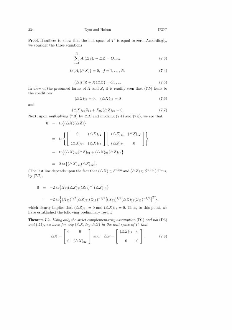
334 Dym and Helton IEOT
Proof. If suffices to show that the null space of T ′ is equal to zero. Accordingly,we consider the three equations
N∑i=1
Ai(�y)i + �Z = On×n. (7.3)
tr{Aj(�X)} = 0, j = 1, . . . , N. (7.4)
(�X)Z + X(�Z) = On×n. (7.5)
In view of the presumed forms of X and Z, it is readily seen that (7.5) leads tothe conditions
(�Z)22 = 0, (�X)11 = 0 (7.6)
and(�X)21Z11 + X22(�Z)21 = 0. (7.7)
Next, upon multiplying (7.3) by �X and invoking (7.4) and (7.6), we see that
0 = tr{(�X)(�Z)
}
= tr
0 (�X)12
(�X)21 (�X)22
(�Z)11 (�Z)12
(�Z)21 0
= tr{(�X)12(�Z)21 + (�X)21(�Z)12
}
= 2 tr{(�X)21(�Z)12
}.
(The last line depends upon the fact that (�X) ∈ Sn×n and (�Z) ∈ Sn×n.) Thus,by (7.7),
0 = −2 tr{X22(�Z)21(Z11)−1(�Z)12
}
= −2 tr{
(X22)1/2(�Z)21(Z11)−1/2[(X22)1/2(�Z)21(Z11)−1/2
]T},
which clearly implies that (�Z)21 = 0 and (�X)12 = 0. Thus, to this point, wehave established the following preliminary result:
Theorem 7.2. Using only the strict complementarity assumption (D1) and not (D3)and (D4), we have for any (�X,�y,�Z) in the null space of T ′ that
�X =
0 0
0 (�X)22
and �Z =
(�Z)11 0
0 0
. (7.8)
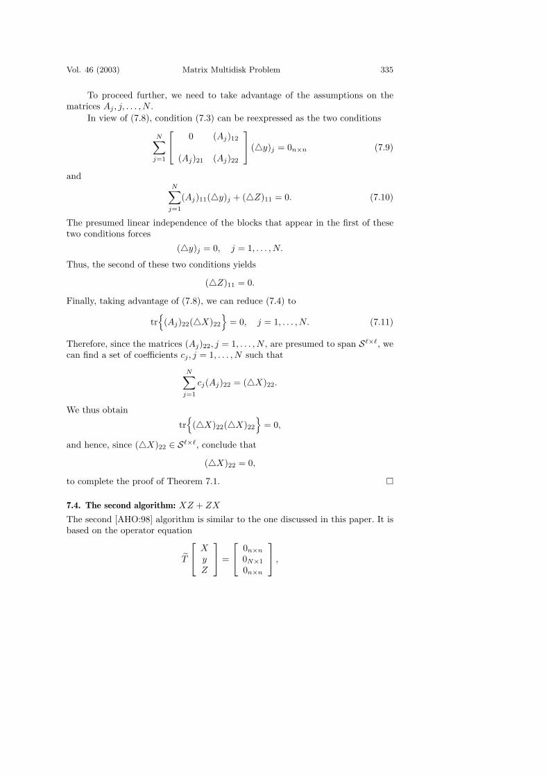
Vol. 46 (2003) Matrix Multidisk Problem 335
To proceed further, we need to take advantage of the assumptions on thematrices Aj , j, . . . , N .
In view of (7.8), condition (7.3) can be reexpressed as the two conditions
N∑j=1
0 (Aj)12
(Aj)21 (Aj)22
(�y)j = 0n×n (7.9)
andN∑
j=1
(Aj)11(�y)j + (�Z)11 = 0. (7.10)
The presumed linear independence of the blocks that appear in the first of thesetwo conditions forces
(�y)j = 0, j = 1, . . . , N.
Thus, the second of these two conditions yields
(�Z)11 = 0.
Finally, taking advantage of (7.8), we can reduce (7.4) to
tr{
(Aj)22(�X)22}
= 0, j = 1, . . . , N. (7.11)
Therefore, since the matrices (Aj)22, j = 1, . . . , N , are presumed to span S��, wecan find a set of coefficients cj , j = 1, . . . , N such that
N∑j=1
cj(Aj)22 = (�X)22.
We thus obtain
tr{
(�X)22(�X)22}
= 0,
and hence, since (�X)22 ∈ S�×�, conclude that
(�X)22 = 0,
to complete the proof of Theorem 7.1. �
7.4. The second algorithm: XZ + ZX
The second [AHO:98] algorithm is similar to the one discussed in this paper. It isbased on the operator equation
T
XyZ
=
0n×n
0N×1
0n×n
,
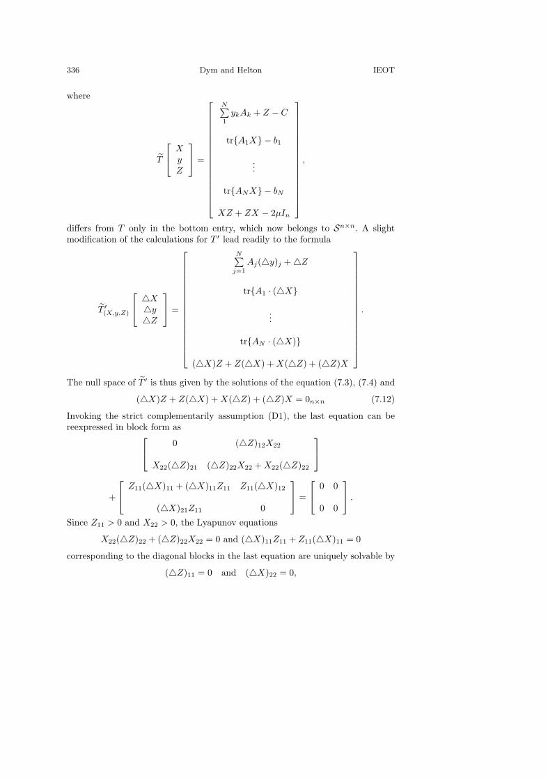
336 Dym and Helton IEOT
where
T
XyZ
=
N∑1
ykAk + Z − C
tr{A1X} − b1
...
tr{ANX} − bN
XZ + ZX − 2µIn
,
differs from T only in the bottom entry, which now belongs to Sn×n. A slightmodification of the calculations for T ′ lead readily to the formula
T ′(X,y,Z)
�X�y�Z
=
N∑j=1
Aj(�y)j + �Z
tr{A1 · (�X}
...
tr{AN · (�X)}
(�X)Z + Z(�X) + X(�Z) + (�Z)X
.
The null space of T ′ is thus given by the solutions of the equation (7.3), (7.4) and
(�X)Z + Z(�X) + X(�Z) + (�Z)X = 0n×n (7.12)
Invoking the strict complementarily assumption (D1), the last equation can bereexpressed in block form as
0 (�Z)12X22
X22(�Z)21 (�Z)22X22 + X22(�Z)22
+
Z11(�X)11 + (�X)11Z11 Z11(�X)12
(�X)21Z11 0
=
0 0
0 0
.
Since Z11 > 0 and X22 > 0, the Lyapunov equations
X22(�Z)22 + (�Z)22X22 = 0 and (�X)11Z11 + Z11(�X)11 = 0
corresponding to the diagonal blocks in the last equation are uniquely solvable by
(�Z)11 = 0 and (�X)22 = 0,
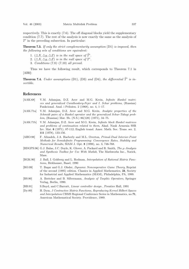
Vol. 46 (2003) Matrix Multidisk Problem 337
respectively. This is exactly (7.6). The off diagonal blocks yield the supplementarycondition (7.7). The rest of the analysis is now exactly the same as the analysis ofT ′ in the preceding subsection. In particular:
Theorem 7.3. If only the strict complementarity assumption (D1) is imposed, thenthe following sets of conditions are equivalent:
1. (�X,�y,�Z) is in the null space of T ′.2. (�X,�y,�Z) is in the null space of T ′.3. Conditions (7.8)–(7.10) all prevail.
Thus we have the following result, which corresponds to Theorem 7.1 in[AH0]:
Theorem 7.4. Under assumptions (D1), (D3) and (D4), the differential T ′ is in-vertible.
References
[AAK:68] V.M. Adamjan, D.Z. Arov and M.G. Krein, Infinite Hankel matri-ces and generalized Caratheodory-Fejer and I. Schur problems, (Russian)Funkcional. Anal. i Prilozen. 2 (1968), no. 4, 1–17.
[AAK:71a] V.M. Adamjan, D.Z. Arov and M.G. Krein, Analytic properties of theSchmidt pairs of a Hankel operator and the generalized Schur-Takagi prob-lem, (Russian) Mat. Sb. (N.S.) 86(128) (1971), 34–75.
[AAK:71b] V.M. Adamjan, D.Z. Arov and M.G. Krein, Infinite block Hankel matricesand problems of continuation related to them, Akad. Nauk Armenia SSRIzv. Mat. 6 (1971), 87-112; English transl. Amer. Math. Soc. Trans. ser. 2,111 (1978), 133-156.
[AHO:98] F. Alizadeh, J.A. Haeberly and M.L. Overton, Primal-Dual Interior-PointMethods for Semidefinite Programming: Convergence Rates, Stability andNumerical Results, SIAM J. Opt. 8 (1998), no. 3, 746-768.
[BDGPS:96] G.J. Balas, J.C. Doyle, K. Glover, A. Packard and R. Smith, The µ-Analysisand Synthesis Toolbox for Use With Matlab, The Mathworks Inc., Natick,Mass.
[BGK:90] J. Ball, I. Gohberg and L. Rodman, Interpolation of Rational Matrix Func-tions, Birkhauser, Basel, 1990
[BO:99] T. Basar and G.J. Olsder, Dynamic Noncooperative Game Theory, Reprintof the second (1995) edition. Classics in Applied Mathematics, 23, Societyfor Industrial and Applied Mathematics (SIAM), Philadelphia, PA, 1999.
[BS:90] A. Bottcher and B. Silbermann, Analysis of Toeplitz Operators, SpringerVerlag, Berlin, 1990.
[BB:91] S.Boyd, and C.Barratt, Linear controller design , Prentice Hall, 1991
[Dy:89] H. Dym, J Contractive Matrix Functions, Reproducing Kernel Hilbert Spacesand Interpolation CBMS Regional Conference Series in Mathematics, no.71,American Mathematical Society. Providence, 1989.
338 Dym and Helton IEOT
[Dy:94] H. Dym, Review of The Commutant Lifting Approach to Interpolation Prob-lems, Bulletin Amer. Math. Soc. 31 (1994), 125-140.
[DG:83] H. Dym and I. Gohberg, Unitary interpolants, factorization indices andinfinite Hankel block matrices, J. Funct. Anal., 54 (1983), 229-289.
[DG:86] H. Dym and I. Gohberg, A maximum entropy principle for contractive in-terpolants, J. Funct. Anal., 65 (1986), 83-125.
[DHM:99] H. Dym, J. W. Helton, and O. Merino, Algorithms for solving multidiskproblems in H∞ optimization, Conference on Decision and Control, 1999.
[DHM:02] H. Dym, J. W. Helton, and O. Merino, Multidisk Problems in H∞ Op-timization: a Method for Analysing Numerical Algorithms, Indiana J., inpress.
[FF:90] C. Foias and A. Frazo, The Commutant Lifting Approach to InterpolationProblems, Birkhauser, Basel, 1990.
[FT:87] C. Foias and A. Tannenbaum, On the Nehari problem for a certain class ofL∞ functions appearing in control theory, J. Funct. Anal., 74 (1987), no. 1.,116-159.
[FO:98] P. Fulcheri and M. Olivi, Matrix rational H2 optimization: a gradient algo-rithm based on Schur analysis, SIAM J. Control Optim., 36 (1998), 2103-2107.
[Ga:81] J.B. Garnett, Bounded Analytic Functions, Academic Press, New York,1981.
[GL:95] M. Green and D.J.N. Limebeer, Linear Robust Control, Prentice Hall, 1995.
[HO:94] J.-P.A. Haeberly and M. L. Overton, Optimizing Eigenvalues of SymmetricDefinite Pencils. Proceedings of the American Control Conference, Balti-more, July 1994.
[Hel:87] J. W. Helton, Operator Theory, Analytic Functions, Matrices, and ElectricalEngineering. CBMS Regional Conference Series in Mathematics. AmericanMathematical Society. Providence, 1987.
[HM:98] J. W. Helton and O. Merino, Classical Control using H∞ Methods: Theory,Optimization and Design, SIAM, Philadelphia, 1998.
[HMW:93] J. W. Helton, O. Merino and T. Walker, Algorithms for Optimizing overAnalytic Functions, Indiana U. Math. J., Vol. 42, No. 3 (1993), 839 - 874.
[HMW:98] J. W. Helton, O. Merino and T. Walker, H∞ Optimization with Plant Uncer-tainty and Semidefinite Programming, I Jour Nonlin Robust Cont. 8 (1998),763-802 (1998).
[HW:prep] J.W. Helton and M.A. Whittlesey, Global Uniqueness Tests for H∞ Optima,in preparation.
[MR:97] A. Megretski and A. Rantzer, System analysis via integral quadratic con-straints. IEEE Trans. Automat. Control 42 (1997), no. 6, 819–830.
[OZ:93] J. G. Owen and G. Zames, Duality theory for MIMO robust disturbancerejection, IEEE Trans. Automat. Control, 38 (1993), no. 5, 743 – 752.
[Pe:98] V.V. Peller, An excursion into the theory of Hankel operators, in: Holomor-phic spaces (Berkeley, CA, 1995), Math. Sci. Res. Inst. Publ., 33, CambridgeUniv. Press, Cambridge, 1998, pp. 65-120.
Vol. 46 (2003) Matrix Multidisk Problem 339
[PY:94] V.V. Peller and N.J. Young, Superoptimal analytic approximations of matrixfunctions, J. Funct. Anal., 120, (1994), 300-343.
[S:97] L.A. Sahknovich Interpolation Theory and its Applications Kluwer, Dor-drecht, 1997
[SC:01] A.J. Sasane and R.F. Curtain, Optimal Hankel norm approximation theoryfor the Pritchard-Salamon class of infinite-dimensional systems, IntegralEquations Operator Theory 39 (2001), no. 1, 98-126.
[VB:96] L. Vandenberghe and S. Boyd, Semidefinite programming, SIAM Review,38 (1996), no.1, 49-95.
[We:94] R. Webster, Convexity, Oxford Univ. Press, Oxford, 1994.
[Wh:00] M.A. Whittlesey, Polynomial hulls and H∞ control for a hypoconvex con-straint, Math. Ann., 317 (2000), no. 4, 677–701.
[Wr:98] S.Wright, Primal Dual Optimization. SIAM. 1998
[Y:86] N.J.Young, The Nevalinna-Pick problem for matrix-valued functions, J. Op-erator Theory, 15(1986), 289-265.
[ZDG:96] K. Zhou, J. Doyle and K Glover, Robust and Optimal Control, New Jersey,1996, Prentice Hall,
[ZTD:92] Y. Zhang, R. A. Tapia and J. E. Dennis, On the super linear and quadraticprimal dual interior point linear programming algorithms, SIAM J. Opt.,2(1992), 304-324.
Harry DymDepartment of MathematicsThe Weizmann Institute of ScienceRehovot 76100, Israel
E-mail: [email protected]
J. William HeltonDepartment of MathematicsUniversity of California, San DiegoLa Jolla, CA 92093-0112USA
E-mail: [email protected]
Submitted: April 23, 2002
To access this journal online:http://www.birkhauser.ch