the membrane shell model in nonlinear elasticity: a ... membrane shell model in nonlinear...

The membrane shell model in nonlinear elasticity:A variational asymptotic derivation

Herve LE DRET1 and Annie RAOULT2

Abstract— We consider a shell-like three-dimensional nonlinearly hyperelastic body and we

let its thickness go to zero. We show, under appropriate hypotheses on the applied loads, that

the deformations that minimize the total energy weakly converge in a Sobolev space toward

deformations that minimize a nonlinear shell membrane energy. The nonlinear shell membrane

energy is obtained by computing theΓ-limit of the sequence of three-dimensional energies.

1 Laboratoire d’Analyse Numerique, Universite Pierre et Marie Curie, 75252 Paris Cedex 05, France2 Laboratoire de Modelisation et Calcul, Universite Joseph Fourier, BP 53, 38041 Grenoble Cedex 9, France

The membrane shell model in nonlinear elasticity 1

1. Introduction

The purpose of this article is to derive nonlinear membrane shell models from genuine three-

dimensional nonlinear elasticity by means of a rigorous convergence result. It is a sequel to a

previous article concerned with planar membranes, see Le Dret and Raoult [1995].

J.C. Simo’s profound interest in the large deformation theory of thin structures is at the origin of

numerous works on the derivation, analysis and approximation of models for shells and rods that

respect the fundamental requirement of continuum mechanics, frame-indifference. These models,

see Simo and Vu-Quoc [1988,1991], Simo and Fox [1989,1992], Simo, Fox and Rifai [1990a,

1990b], Simo and Tarnow [1994] for instance, rely on a kinematic assumption on the possible

deformed configurations of the body. In this framework, shells are one-director Cosserat structures.

The shell model constructed in Simo and Fox [1989] is fully nonlinear, frame-indifferent and couples

membrane, bending and shearing effects together. Recent results on the numerical approximation

and on the construction of such a model are given in Carrive-Bedouani, Le Tallec and Mouro

[1995], Carrive-Bedouani [1995]. Important contributions to the formulation of classical nonlinear

shell theory using the Cosserat hypothesis as well as thorough and comprehensive analysis of these

models can be found ine.g.Ericksen and Truesdell [1958], Naghdi [1972], Green and Naghdi

[1974], Antman [1976a, 1976b, 1995].

A complementary approach to thin elastic structures theory is that of formal asymptotic expan-

sions in powers of the thickness pioneered by Friedrichs and Dressler [1961] and Goldenveizer

[1963] and later recast in a modern functional framework by Ciarlet and Destuynder [1979a, 1979b],

Ciarlet [1980] and in the case of shells Destuynder [1980]. This approach also led to numerous

developments, see Ciarlet [1990] for a bibliography. A one year stay of the second author at the

Division of Applied Mechanics at Stanford University provided the opportunity to try and bridge the

two approaches. More specifically, the goal was to investigate whether the asymptotic expansion

method applied to thin bodies could lead to frame-indifferent limit models.

This objective is attained in Fox, Raoult and Simo [1993] where, for simplicity, the case of

plate-like—rather than shell-like—bodies is treated and where the nonlinear material is the Saint

Venant-Kirchhoff material. It is shown that a hierarchy of two-dimensional models can be derived

from the nonlinear system of three-dimensional elasticity by a formal asymptotic expansion. The

type of limit model thus obtained depends on the order of magnitude of the external loads. The first

two models in the hierarchy are a nonlinear membrane plate model and a nonlinear inextensional

bending model for smaller loads. Both models are quasilinear and frame-indifferent. The membrane

model is also obtained by Karwowski [1993]. By lowering again the order of magnitude of the loads,

one recovers semilinear plate models that had been previously derived by Ciarlet and Destuynder

[1979b], Ciarlet [1980] for the von Karman equations and Raoult [1988] in the dynamical case by

analogous formal expansions. Note that these models are no longer frame-indifferent.

2 H. Le Dret & A. Raoult

Although establishing the grounds for an asymptotic justification of invariant plate models,

the method of Fox, Raoult and Simo [1993] is purely formal. It was the purpose of the work

by Le Dret and Raoult [1993, 1995] to provide a rigorous proof of convergence to a nonlinear

membrane model. In this work, as in Fox, Raoult and Simo [1993], only plate-like bodies are

considered. The assumptions on the external loads are those of Fox, Raoult and Simo [1993],

but the results are obtained for a general hyperelastic material. The main mathematical tool is

Γ-convergence theory, a systematic way of analysing the convergence of minimizers of a sequence

of problems of the Calculus of Variations. Ideas fromΓ-convergence theory had been previously

introduced in the context of lower-dimensional theories in nonlinear elasticity by Acerbi, Buttazzo

and Percivale [1991] for nonlinearly elastic strings. Their method was extended to nonlinear planar

membranes in a preprint by Percivale [1991] recently drawn to the authors’ attention. Note that

in the case of strings the limit model is one-dimensional and thus convexity arguments can be

used that are not sufficient in the two-dimensional case. Let us briefly recall the limit membrane

model obtained in Le Dret and Raoult [1993, 1995], see also Percivale [1991]. Starting from a

three-dimensional stored energy functionW defined on three-dimensional deformation gradients,

i.e., 3×3 matrices, the limit membrane energy density, which is defined on membrane deformation

gradients,i.e., 3 × 2 matrices, is constructed in two steps. FirstW is minimized with respect

to the third column of its matrix argument, then the resulting function is quasiconvexified. It is

worth mentioning that, except in some very special cases, this quasiconvexification step cannot be

skipped. In the case of the Saint Venant-Kirchhoff density, the quasiconvexification is carried out

explicitly in Le Dret and Raoult [1995]. A quite surprising consequence of this calculation is that

the formal limit membrane energy of Fox, Raoult and Simo [1993] only coincides with the rigorous

limit energy on a compact subset of the set of3× 2 matrices.

The present article extends the analysis of Le Dret and Raoult [1995] to the case of shells. Let us

mention other recent works in the field of asymptotic justification and analysis of lower-dimensional

linear or nonlinear shell models: Sanchez-Palencia [1989a, 1989b, 1990], Ciarlet and Lods [1994],

Ciarlet, Lods and Miara [1994], Miara [1994].

An overview of the article is as follows. Section 2 is devoted to introducing the geometrical

notation for a shell with mid-surfaceS and thickness2ε in its reference configurationΩε. We

assume that the shell is made of a hyperelastic homogeneous material with stored energy function

W . In Section 3, we state the equilibrium problem for the shell as an energy minimization problem

over a set of admissible deformations included in the Sobolev spaceW 1,p(Ωε;R3). To study the

asymptotic behavior of the corresponding energy minimizers whenε→ 0, we define an equivalent

minimization problem set on a straight cylindrical domainΩ = ω × ]−1, 1[ of R3 independent of

ε. This is achieved by transporting the deformations and the external loads through a chart and

rescaling them. As opposed to the planar case, the geometry of the shell intervenes in the expression

of the rescaled hyperelastic energies through the Jacobian matrix of the change of coordinates. This


matrix depends onε and appears notably inside the argument of the stored energy density.

In Section 4, we give our first convergence result expressed in terms of rescaled displacements.

We determine theΓ-limit of the sequence of rescaled energies. The construction of the limit energy

density extends that of the planar case. Note however that the nontrivial geometry of the shell

causes the limit energy to depend on the pointx ∈ ω even for a homogeneous three-dimensional

material.

In Section 5, we translate theΓ-convergence result of Section 4 in terms of deformations and

show that the minimizing deformations weakly converge inW 1,p(Ω;R3) towards deformations

that minimize a limit nonlinear shell energy. The limit deformations depend on two space variables

only (they are identified with functions defined on the transported mid-surfaceω). The limit elastic

energy of a deformationϕ depends on its first derivatives and thus does not incorporate bending

effects associated with curvature nor shear effects. Consequently, it is a membrane energy. Let

us emphasize the fact that, contrarily to methods relying on Cosserat assumptions, our analysis

provides an exact formula for deriving the limit energy, hence the membrane constitutive law, from

the three-dimensional energyW . Furthermore, we give an intrinsic formulation of the membrane

minimization problem and an intrinsic expression of the nonlinear membrane energy by transporting

the obtained result back on the reference surfaceS. The stored energy depends on a deformationϕ

defined onS only through its gradient (for a definition of this gradient, see Section 5). It depends

on the current point ofS, but only through the normal vector toS at this point.

In Section 6, we study how the limit membrane shell energy inherits the invariance properties

of the three-dimensional energy. In particular, it is shown that frame-indifference is preserved and

that the shell energy depends on the deformation only through the deformed metric. Moreover, if

W has a global zero minimum atF = I, the corresponding membrane shell energy is zero for

compressive states. Isotropy is also preserved. In this case, the membrane stored energy does no

longer depend on the normal vector to the reference surfaceS and depends on the deformation

only through the principal stretches.

The second author is indebted to J.C. Simo for inviting her to spend a sabbatical year at the

Division of Applied Mechanics at Stanford University in 1990–1991. Her work owes much to J.C.

Simo’s brilliance and enthusiasm.

2. Geometrical preliminaries

The summation convention is assumed throughout this article, unless otherwise specified. Greek

indices take their values in the set1, 2 and Latin indices take their values in the set1, 2, 3. Let

(e1, e2, e3) be the canonical orthonormal basis of the Euclidean spaceR3. The norm of a vector

of R3 will be denoted by‖u‖, the scalar product of two vectors ofR3 by u · v and their vector

product byu ∧ v. In the sequel, we will identifyR2 with the plane spanned by the vectorse1 and

e2. Accordingly and depending on the context,x will denote a generic point ofR2 orR3. LetM3


be the space of real3× 3 matrices endowed with the usual Euclidean norm‖F‖ =√

tr (FTF ).For anyzi ∈ R3, i = 1, 2, 3, we note(z1|z2|z3) the matrix whosei-th column consists of the

components ofzi in the canonical basis.

We assume that the midsurfaceS is a bounded, two-dimensional,C2-submanifold ofR3, which,

for simplicity, admits an atlas consisting of one chart only. Letψ be this chart. It is thus a

C2-mapping from a bounded, open setω ⊂ R2 intoR3 which is a global diffeomorphism between

ω andS. We assume thatω has a Lipschitz boundary and thatψ admits an extension toω into a

C2(ω;R3)-function.

Let aα(x) = ∂ψ∂xα

(x) be the covariant basis vectors of the tangent planeTψ(x)S, associated with

the chartψ. These vectors are linearly independent onω. We assume furthermore that there exists

δ > 0 such that

‖a1(x) ∧ a2(x)‖ ≥ δ on ω. (1)

We then definea3(x) = a1(x)∧a2(x)‖a1(x)∧a2(x)‖ ∈ C1(ω;S2), which is a unit normal vector toTψ(x)S.

If no confusion may arise from it, we will writea3(x) for a3(x) at point x = ψ(x), since it is

important to remember thata3 is actually chart-independent (modulo multiplication by−1). The

contravariant basis vectors are defined by the relationsaα(x) ∈ Tψ(x)S, aα(x) · aβ(x) = δαβ and

a3(x) = a3(x).

Using this notation, we letA(x) = (a1(x)|a2(x)|a3(x)). This matrix is everywhere nonsingular

on ω and its inverse is given byA−1(x) = (a1(x)|a2(x)|a3(x))T . Note that due to our choice of

unit normal vector,detA(x) = ‖a1(x) ∧ a2(x)‖ ≥ δ > 0 on ω. Thus, there exists a constantC

such that

∀x ∈ ω, ‖A−1(x)‖ ≤ C. (2)

The functiondetA(x) also satisfies

detA(x) = ‖ cof A(x)e3‖ =√a(x) (3)

wherea is the determinant of the metric onS expressed in the chartψ.

Forε > 0, we consider the setΩε defined by

Ωε = y ∈ R3;∃ x ∈ S, y = x+ ηa3(x) with |η| < ε. (4)

This set is the reference configuration of a shell of thickness2ε. Due to our regularity hypothesis

on S there exists aC1-orthogonal projection mappingΠ : Ωε → S if ε is small enough, which will

be understood thereafter. Anyy in Ωε can be uniquely decomposed asy = Π(y) + [(y − Π(y)) ·a3(Π(y))]a3(Π(y)). With this notation,(x1, x2) = ψ−1(Π(y)) andx3 = (y − Π(y)) · a3(Π(y))define the natural curvilinear coordinate system inΩε that is associated with the chartψ of the

midsurface. If

Ωε = x ∈ R3; (x1, x2) ∈ ω, |x3| < ε, (5)


then theC1-diffeomorphismΨ : Ωε → Ωε defined by

Ψ(x) = ψ(x1, x2) + x3a3(x1, x2) (6)

is the inverse of this change of coordinates. Its gradient is the matrix

∇Ψ(x) = A(x1, x2) + x3(∂1a3(x1, x2)|∂2a3(x1, x2)|0). (7)

Naturally, this gradient is everywhere nonsingular as soon asε is small enough. In the context of

nonlinear elasticity, the mappingΨ−1 can also be viewed as a change of reference configuration

for the shell (Ψ is orientation preserving).

3. The three-dimensional and rescaled problems

We assume that the shells are made of the same hyperelastic homogeneous material whose stored

energy function is denoted byW . The functionW :M3 → R is continuous and satisfies the growth

and coercivity hypotheses∃C > 0,∃ p ∈ ]1,+∞[,∀F ∈M3, |W (F )| ≤ C(1 + ‖F‖p),

∃α > 0,∃β ≥ 0,∀F ∈M3,W (F ) ≥ α‖F‖p − β,

∀F, F ′ ∈M3, |W (F )−W (F ′)| ≤ C(1 + ‖F‖p−1 + ‖F ′‖p−1)‖F − F ′‖.

(8)

Assumption (8)3 was not needed in the case of planar membranes considered in Le Dret and

Raoult [1995]. It is however quite natural. In particular, ifW is quasiconvex (8)1 implies (8)3,

cf. Marcellini [1985]. Assumption (8)3 also holds true ifW is continuously differentiable and its

derivative grows as‖F‖p−1 at infinity.

Let S±ε = ω × ±ε and defineS±ε = Ψ(S±ε ) to be the top and bottom surfaces of the

shell. For simplicity, we assume that the shells are solely submitted to the action of dead loading

surface traction densitiesgε ∈ Lq(S±ε ;R3) with 1/p + 1/q = 1. Taking body forces and lateral

forces into account is straightforward. An example of live loads is detailed in the appendix. Let

Γε = ∂ω×]−ε, ε[ andΓε = Ψ(Γε) be the lateral surface ofΩε. We assume that the deformations of

the shells satisfy a boundary condition of place onΓε. The equilibrium problem may be formulated

as a minimization problem:

Find φε ∈ Φε such thatIε(φε) = infϕ∈Φε

Iε(ϕ), (9)

where the total energyIε is

Iε(ϕ) =∫

Ωε

W (∇ϕ) dx−∫Sε

gε · ϕ dσε, (10)


dσε is the surface element onSε and the set of admissible deformations is

Φε = ϕ ∈W 1,p(Ωε;R3); ϕ(x) = x on Γε. (11)

See Wang and Truesdell [1973], Marsden and Hughes [1983] or Ciarlet [1988], among others, for

general references on three-dimensional nonlinear elasticity. A key-ingredient in existence proofs

using the direct method of the calculus of variations is the sequential weak lower semi-continuity

of the energy functionalIε onW 1,p(Ωε;R3). Under assumptions (8), it is known that the energy

functionalIε in problem (9) is sequentially weakly lower semi-continuous onW 1,p(Ωε;R3) if and

only if the functionW is quasiconvex,i.e.,

∀F ∈M3,∀ θ ∈W 1,∞0 (O;R3),

∫O

W (F +∇θ(x)) dx ≥ (measO)W (F ), (12)

whereO is any bounded domain ofR3, see Morrey [1952], Acerbi and Fusco [1984], Da-

corogna [1989] and the references therein. Problem (9) was solved in the more physical case

W (F ) = +∞ if detF ≤ 0 andW (F ) → +∞ whendetF → 0+ by Ball [1977], under an

assumption of polyconvexity ofW , a notion more restrictive than quasiconvexity, plus appropriate

growth and coercivity assumptions. For our purposes here, it is not desirable to assume at the onset

thatW is quasiconvex or polyconvex. There are two reasons for this. First of all, the zero thickness

limit model we obtain always involves a quasiconvexification, which has to be effected whether

W is quasiconvex or not. Secondly, we do not want to rule out important examples, such as the

Saint Venant-Kirchhoff stored energy function which is neither polyconvex nor quasiconvex, see

Raoult [1986]. Consequently, wedo notassume thatW is quasiconvex and problem (9) may well

not possess any solutions. Naturally, if it does have solutions which are thus actual equilibrium

deformations of the bodies, our results apply to these deformations.

Let us thus be given a diagonal minimizing sequenceφε for the sequence of energiesIε over the

setsΦε. More specifically, we assume that

φε ∈ Φε, Iε(φε) ≤ infϕ∈Φε

Iε(ϕ) + εh(ε), (13)

whereh is a positive function such thath(ε) → 0 whenε → 0. Such a sequence always exists

and, if the minimization problems have solutions,φε may be chosen to be such a solution.

As in the case of a planar membrane, we assume that‖gε‖Lq(S±ε ;R3) ≤ Cε where the constant

C does not depend onε. If we also considered body force densities or lateral traction densities, we

would assume them to be of the order of1 so that all force resultants would be of the order ofε (in

particular, the weight of the material is allowed). This is essential in order to obtain a membrane

model in the limit, see Le Dret and Raoult [1995], Fox, Raoult and Simo [1993] for a discussion of

this observation.


We first rewrite problem (9) in the curvilinear coordinate system or, equivalently, we consider

Ωε as a new reference configuration. Note that this configuration is not homogeneous anymore.

If ϕ is a deformation of the shell in its first reference configuration, we thus define for almost all

x ∈ Ωε,ϕ(x) = ϕ(Ψ(x)), (14)

and the set of admissible deformations becomes

Φε = ϕ ∈W 1,p(Ωε;R3);ϕ(x) = Ψ(x) onΓε. (15)

Similarly, we set for almost allx ∈ S±ε

gε(x) = gε(Ψ(x)), (16)

and by definingIε(ϕ) = Iε(ϕ) to be the energy in the new reference configuration,i.e.,

Iε(ϕ) =∫

Ωε

W (∇ϕ(x)∇Ψ(x)−1) det(∇Ψ(x)) dx−∫S±ε

gε(x)·ϕ(x)‖ cof∇Ψ(x)e3‖ dσε, (17)

we obtain

φε ∈ Φε, Iε(φε) ≤ infϕ∈Φε

Iε(ϕ) + εh(ε). (18)

All these definitions may also be rewritten in terms of displacementsv(x) = ϕ(x)−Ψ(x).

We now are in a position to rescale the problem. LetΩ = Ω1, Γ = Γ1 and S± = S±1and define a rescaling operatorΘε by (Θεϕ)(x1, x2, x3) = ϕ(x1, x2, εx3). Let φ(ε) = Θεφ

ε,

Ψ(ε)(x) = ΘεΨ andg(ε)(x) = Θεgε. The rescaled displacementu(ε) = φ(ε)−Ψ(ε) belongs to

V = W 1,pΓ (Ω;R3). We rescale the energies by settingI(ε)(ϕ) = ε−1Iε(Θ−1

ε ϕ), i.e.,

I(ε)(ϕ) =∫

Ω

W((∂1ϕ

∣∣∣∂2ϕ∣∣∣∂3ϕ

ε

)A(ε)−1

)detA(ε) dx−

∫S±

ε−1g(ε) · ϕ‖ cof A(ε)e3‖ dσ,(19)

with the notation:

A(ε)(x) = ∇Ψ(x1, x2, εx3) = A(x1, x2) + εx3(∂1a3(x1, x2)|∂2a3(x1, x2)|0). (20)

In terms of the rescaled displacements, the rescaled energy reads:

J(ε)(v) =∫

Ω

W((∂1v∣∣∣∂2v

∣∣∣∂3v

ε

)A(ε)−1 + I

)detA(ε) dx

−∫S±

ε−1g(ε) · (Ψ(ε) + v)‖ cof A(ε)e3‖ dσ.(21)

It is immediate that

J(ε)(u(ε)) ≤ infv∈V

J(ε)(v) + h(ε). (22)


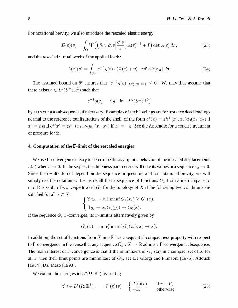
For notational brevity, we also introduce the rescaled elastic energy:

E(ε)(v) =∫

Ω

W((∂1v∣∣∣∂2v

∣∣∣∂3v

ε

)A(ε)−1 + I

)detA(ε) dx, (23)

and the rescaled virtual work of the applied loads:

L(ε)(v) =∫S±

ε−1g(ε) · (Ψ(ε) + v)‖ cof A(ε)e3‖ dσ. (24)

The assumed bound ongε ensures that‖ε−1g(ε)‖Lq(S±;R3) ≤ C. We may thus assume that

there existsg ∈ Lq(S±;R3) such that

ε−1g(ε) − g in Lq(S±;R3)

by extracting a subsequence, if necessary. Examples of such loadings are for instance dead loadings

normal to the reference configurations of the shell, of the formgε(x) = εh+(x1, x2)a3(x1, x2) if

x3 = ε andgε(x) = εh−(x1, x2)a3(x1, x2) if x3 = −ε. See the Appendix for a concise treatment

of pressure loads.

4. Computation of theΓΓΓΓΓ-limit of the rescaled energies

We useΓ-convergence theory to determine the asymptotic behavior of the rescaled displacements

u(ε) whenε→ 0. In the sequel, the thickness parameterεwill take its values in a sequenceεn → 0.

Since the results do not depend on the sequence in question, and for notational brevity, we will

simply use the notationε. Let us recall that a sequence of functionsGε from a metric spaceX

into R is said toΓ-converge towardG0 for the topology ofX if the following two conditions are

satisfied for allx ∈ X: ∀xε → x, lim inf Gε(xε) ≥ G0(x),

∃ yε → x,Gε(yε)→ G0(x).

If the sequenceGε Γ-converges, itsΓ-limit is alternatively given by

G0(x) = minlim inf Gε(xε);xε → x.

In addition, the set of functions fromX into R has a sequential compactness property with respect

to Γ-convergence in the sense that any sequenceGε : X → R admits aΓ-convergent subsequence.

The main interest ofΓ-convergence is that if the minimizers ofGε stay in a compact set ofX for

all ε, then their limit points are minimizers ofG0, see De Giorgi and Franzoni [1975], Attouch

[1984], Dal Maso [1993].

We extend the energies toLp(Ω;R3) by setting

∀ v ∈ Lp(Ω;R3), J∗(ε)(v) =J(ε)(v) if v ∈ V ,+∞ otherwise.

(25)


Let us now proceed to compute theΓ-limit of the sequenceJ∗(ε) for the strong topology of

Lp(Ω;R3). LetM3,2 be the space of3× 2 real matrices endowed with the usual Euclidean norm

‖F‖ =√

tr (FT F ). We note(z1|z2) the matrix ofM3,2 whoseα-th column is composed of the

components ofzα ∈ R3 in the canonical basis. For allF = (z1|z2) ∈ M3,2 andz ∈ R3, we also

note(F |z) the matrix whose first two columns arez1 andz2 and whose third column isz.

Let us introduce a functionW0: ω ×M3,2 → R

W0(x, F ) = infz∈R3

W ((F |z)A−1(x)). (26)

Due to the coercivity assumption (8)2, it is clear that this function is well defined. Besides, since

W is continuous, the infimum is attained. Let us briefly state a few properties ofW0: The function

W0 is continuous onω ×M3,2 and satisfies the growth and coercivity estimates∃C ′ > 0,∀ F ∈M3,2,∀x ∈ ω, |W0(x, F )| ≤ C ′(1 + ‖F‖p),

∃α′ > 0,∃β′ ≥ 0,∀ F ∈M3,2,∀x ∈ ω,W0(x, F ) ≥ α′‖F‖p − β′.(27)

See Le Dret and Raoult [1995] for a proof in the planar case. We use here in addition the continuity

of A andA−1 on ω.

Let QW0 = supZ: ω ×M3,2 → R, Z quasiconvex, Z ≤ W0 be the quasiconvex envelope

of W0, see Dacorogna [1982] for the definition and properties of quasiconvex functions and

quasiconvex envelopes. Recall that a functionZ of x andF is quasiconvex if it satisfies

∀x0 ∈ ω,∀ F ∈M3,∀ θ ∈W 1,∞0 (O;R3),

∫O

Z(x0, F +∇θ(x)) dx ≥ (measO)Z(x0, F ),

(28)

whereO is any bounded domain ofR2. This is the same definition as (12) in the3 × 2 case with

the variablex0 frozen. We introduce the space

VM = v ∈ V ; ∂3v = 0, (29)

which we call the space of membrane displacements. This space is canonically isomorphic to

W 1,p0 (ω;R3) and we letv denote the element ofW 1,p

0 (ω;R3) that is associated withv ∈ VM

through this isomorphism. The expression of theΓ-limit of the sequenceJ∗(ε) is given in the

following theorem.

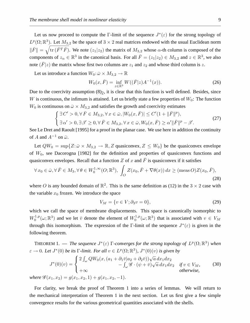
THEOREM1. — The sequenceJ∗(ε) Γ-converges for the strong topology ofLp(Ω;R3) when

ε→ 0. LetJ∗(0) be itsΓ-limit. For all v ∈ Lp(Ω;R3), J∗(0)(v) is given by

J∗(0)(v) =

2∫ωQW0(x, (a1 + ∂1v|a2 + ∂2v))

√a dx1dx2

−∫ω

G · (ψ + v)√a dx1dx2 if v ∈ VM ,

+∞ otherwise,(30)

whereG (x1, x2) = g(x1, x2, 1) + g(x1, x2,−1).

For clarity, we break the proof of Theorem 1 into a series of lemmas. We will return to

the mechanical interpretation of Theorem 1 in the next section. Let us first give a few simple

convergence results for the various geometrical quantities associated with the shells.


LEMMA 2. — The matrixA(ε) satisfies

detA(ε) = ‖ cof A(ε)e3‖ →√a in C0(Ω), A(ε)−1 → A−1 in C0(Ω;M3) (31)

and the rescaled chartΨ(ε) satisfies

Ψ(ε)→ Ψ(0) in C0(Ω;R3) (32)

whereΨ(0)(x1, x2, x3) = ψ(x1, x2).

We now extract aΓ-convergent subsequence, still denotedJ∗(ε), and callJ∗(0) its Γ-limit. The

uniqueness ofJ∗(0) will make the extraction of this subsequence superfluousa posteriori.

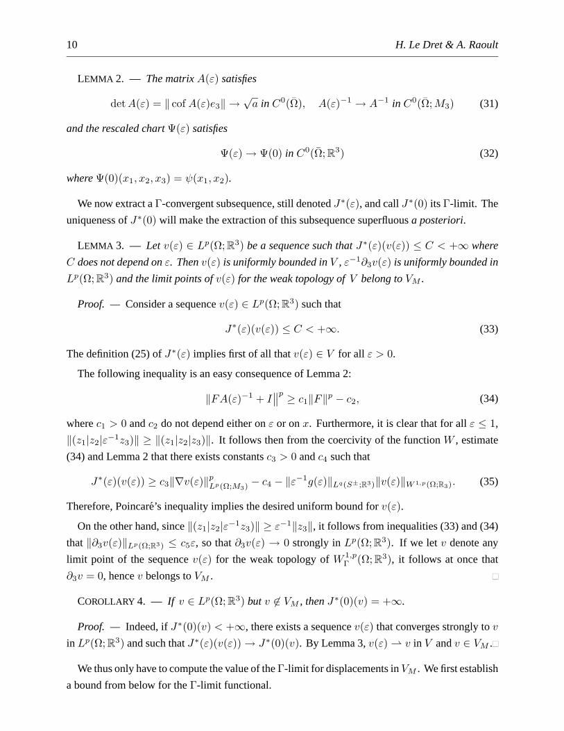
LEMMA 3. — Let v(ε) ∈ Lp(Ω;R3) be a sequence such thatJ∗(ε)(v(ε)) ≤ C < +∞ where

C does not depend onε. Thenv(ε) is uniformly bounded inV , ε−1∂3v(ε) is uniformly bounded in

Lp(Ω;R3) and the limit points ofv(ε) for the weak topology ofV belong toVM .

Proof. — Consider a sequencev(ε) ∈ Lp(Ω;R3) such that

J∗(ε)(v(ε)) ≤ C < +∞. (33)

The definition (25) ofJ∗(ε) implies first of all thatv(ε) ∈ V for all ε > 0.

The following inequality is an easy consequence of Lemma 2:

‖FA(ε)−1 + I∥∥p ≥ c1‖F‖p − c2, (34)

wherec1 > 0 andc2 do not depend either onε or onx. Furthermore, it is clear that for allε ≤ 1,

‖(z1|z2|ε−1z3)‖ ≥ ‖(z1|z2|z3)‖. It follows then from the coercivity of the functionW , estimate

(34) and Lemma 2 that there exists constantsc3 > 0 andc4 such that

J∗(ε)(v(ε)) ≥ c3‖∇v(ε)‖pLp(Ω;M3) − c4 − ‖ε−1g(ε)‖Lq(S±;R3)‖v(ε)‖W 1,p(Ω;R3). (35)

Therefore, Poincare’s inequality implies the desired uniform bound forv(ε).

On the other hand, since‖(z1|z2|ε−1z3)‖ ≥ ε−1‖z3‖, it follows from inequalities (33) and (34)

that‖∂3v(ε)‖Lp(Ω;R3) ≤ c5ε, so that∂3v(ε) → 0 strongly inLp(Ω;R3). If we let v denote any

limit point of the sequencev(ε) for the weak topology ofW 1,pΓ (Ω;R3), it follows at once that

∂3v = 0, hencev belongs toVM .

COROLLARY 4. — If v ∈ Lp(Ω;R3) but v 6∈ VM , thenJ∗(0)(v) = +∞.

Proof. — Indeed, ifJ∗(0)(v) < +∞, there exists a sequencev(ε) that converges strongly tov

in Lp(Ω;R3) and such thatJ∗(ε)(v(ε))→ J∗(0)(v). By Lemma 3,v(ε) v in V andv ∈ VM .

We thus only have to compute the value of theΓ-limit for displacements inVM . We first establish

a bound from below for theΓ-limit functional.


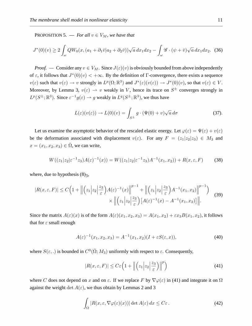
PROPOSITION5. — For all v ∈ VM , we have that

J∗(0)(v) ≥ 2∫ω

QW0(x, (a1 + ∂1v|a2 + ∂2v))√a dx1dx2 −

∫ω

G · (ψ + v)√a dx1dx2. (36)

Proof. — Consider anyv ∈ VM . SinceJ(ε)(v) is obviously bounded from above independently

of ε, it follows thatJ∗(0)(v) < +∞. By the definition ofΓ-convergence, there exists a sequence

v(ε) such thatv(ε) → v strongly inLp(Ω;R3) andJ∗(ε)(v(ε)) → J∗(0)(v), so thatv(ε) ∈ V .

Moreover, by Lemma 3,v(ε) v weakly in V , hence its trace onS± converges strongly in

Lp(S±;R3). Sinceε−1g(ε) g weakly inLq(S±;R3), we thus have

L(ε)(v(ε))→ L(0)(v) =∫S±

g · (Ψ(0) + v)√a dσ (37).

Let us examine the asymptotic behavior of the rescaled elastic energy. Letϕ(ε) = Ψ(ε) + v(ε)be the deformation associated with displacementv(ε). For anyF = (z1|z2|z3) ∈ M3 and

x = (x1, x2, x3) ∈ Ω, we can write,

W ((z1|z2|ε−1z3)A(ε)−1(x)) = W ((z1|z2|ε−1z3)A−1(x1, x2)) +R(x, ε, F ) (38)

where, due to hypothesis (8)3,

|R(x, ε, F )| ≤ C(

1 +∥∥∥(z1

∣∣∣z2

∣∣∣z3

ε

)A(ε)−1(x)

∥∥∥p−1

+∥∥∥(z1

∣∣∣z2

∣∣∣z3

ε

)A−1(x1, x2)

∥∥∥p−1)×∥∥∥(z1

∣∣∣z2

∣∣∣z3

ε

)[A(ε)−1(x)−A−1(x1, x2)

]∥∥∥. (39)

Since the matrixA(ε)(x) is of the formA(ε)(x1, x2, x3) = A(x1, x2) + εx3B(x1, x2), it follows

that forε small enough

A(ε)−1(x1, x2, x3) = A−1(x1, x2)(I + εS(ε, x)), (40)

whereS(ε, .) is bounded inC0(Ω;M3) uniformly with respect toε. Consequently,

|R(x, ε, F )| ≤ Cε(

1 +∥∥∥(z1

∣∣∣z2

∣∣∣z3

ε

)∥∥∥p) (41)

whereC does not depend onx and onε. If we replaceF by∇ϕ(ε) in (41) and integrate it onΩagainst the weightdetA(ε), we thus obtain by Lemmas 2 and 3∫

Ω

|R(x, ε,∇ϕ(ε)(x))|detA(ε) dx ≤ Cε . (42)


We now infer from equation (38) and the definition (26) ofW0 that

E(ε)(v(ε)) ≥∫

Ω

W0((x1, x2), (∂1ϕ(ε)|∂2ϕ(ε))) detA(ε) dx

+∫

Ω

R(x, ε,∇ϕ(ε)(x)) detA(ε) dx

≥∫

Ω

QW0((x1, x2), (∂1ϕ(ε)|∂2ϕ(ε))) detA(ε) dx

+∫

Ω

R(x, ε,∇ϕ(ε)(x)) detA(ε) dx.

(43)

Therefore, estimate (42) implies that

limε→0

E(ε)(v(ε)) ≥ lim infε→0

∫Ω

QW0((x1, x2), (∂1ϕ(ε)|∂2ϕ(ε))) detA(ε) dx

= lim infε→0

∫Ω

QW0((x1, x2), (∂1ϕ(ε)|∂2ϕ(ε))) detAdx(44)

sincedetA(ε)→ detA in C0(Ω). LetG:W 1,p(Ω;R3)→ R be defined by

G(ϕ) =∫

Ω

QW0((x1, x2), (∂1ϕ|∂2ϕ)) detA(x1, x2) dx. (45)

We define a functionZ: Ω×M3 → R byZ(x, (z1|z2|z3))=QW0((x1, x2), (z1|z2)) detA(x1, x2)so thatG(ϕ) =

∫ΩZ(x,∇ϕ(x)) dx. SinceQW0 is quasiconvex, it is easy to see thatZ is

also quasiconvex, see Le Dret and Raoult [1995]. Moreover,Z is continuous, bounded below

and satisfies the growth condition (8)1 sinceQW0 satisfies (27)1. Therefore, the functionG is

sequentially weakly lower semi-continuous onW 1,p(Ω;R3), see Acerbi and Fusco [1984], Meyers

[1965], Dacorogna [1989]. Consequently, asϕ(ε) ϕ = Ψ(0) + v in W 1,p(Ω;R3),

limε→0

E(ε)(v(ε)) ≥ lim infε→0

G(ϕ(ε)) ≥ G(ϕ)

= 2∫ω

QW0((x1, x2), (a1 + ∂1v|a2 + ∂2v))√a(x1, x2) dx1dx2,

(46)

and the proof is complete.

Let us now turn to proving the reverse inequality. We first recall a technical lemma, see Dal

Maso [1993], Le Dret and Raoult [1995].

LEMMA 6. — Let X → Y be two Banach spaces such thatX is reflexive and compactly

embedded inY . Consider a functionalG:X → R such that for allv ∈ X, G(v) ≥ g(‖v‖X)whereg is such thatg(t) → +∞ as t → +∞. LetG∗:Y → R be defined byG∗(v) = G(v) if

v ∈ X, G∗(v) = +∞ otherwise. LetΓ-G denote the sequential lower semi-continuous envelope


of G for the weak topology ofX andΓ-G∗ denote the lower semi-continuous envelope ofG∗ for

the strong topology ofY . ThenΓ-G∗ = (Γ-G)∗.

PROPOSITION7. — For all v ∈ VM , the following estimate holds true:

J∗(0)(v) ≤ 2∫ω

QW0((x1, x2), (a1 + ∂1v|a2 + ∂2v))√a dx1dx2 −

∫ω

G · (ψ + v)√a dx1dx2.

(47)

Proof. — Let us considerv ∈ VM . For allw ∈W 1,p0 (ω;R3), we define a displacement

v(ε)(x) = v(x1, x2) + εx3w(x1, x2), (48)

and the associated deformationϕ(ε) = Ψ(ε) + v(ε) = ϕ + εx3(a3 + w), with ϕ = ψ + v.

Obviously,v(ε)→ v strongly inW 1,p(Ω;R3). Let us examine the limit behavior of the sequence

J∗(ε)(v(ε)). By the dominated convergence theorem and the growth estimate, it is clear that

E(ε)(v(ε)) =∫

Ω

W ((∂1ϕ(ε)|∂2ϕ(ε)|a3 + w)A(ε)−1) detA(ε) dx

→2∫ω

W ((∂1ϕ|∂2ϕ|a3 + w)A−1) detAdx1dx2

(49)

whenε→ 0. Consequently,

J∗(ε)(v(ε)) −→ 2∫ω

W ((∂1ϕ|∂2ϕ|a3+w)A−1) detAdx1dx2−∫ω

G ·(ψ+v)√a dx1dx2. (50)

As this is true for allw ∈W 1,p0 (ω;R3), it follows from the definition ofΓ-convergence that

J∗(0)(v) ≤ infw∈W 1,p

0 (ω;R3)

2∫ω

W ((∂1ϕ|∂2ϕ|a3 + w)A−1) detAdx1dx2

−∫ω

G · (ψ+v)√a dx1dx2.

(51)

We remark that in inequality (51), the infimum overW 1,p0 (ω;R3) can be replaced by the infimum

overLp(ω;R3), by the density ofW 1,p0 (ω;R3) in Lp(ω;R3) and by the dominated convergence

theorem. The functiong:ω × R3 → R, g(x, z) = W ((∂1ϕ|∂2ϕ|a3 + z)A−1) is a Caratheodory

function. Hence, the measurable selection lemma,cf.Ekeland and Temam [1974], shows that there

exists a measurable functionw0 such that

W0(x, (∂1ϕ(x)|∂2ϕ(x))) = W ((∂1ϕ(x)|∂2ϕ(x)|a3(x) + w0(x))A−1(x)) (52)

for almost allx ∈ ω. Due to the coercivity estimate,w0 ∈ Lp(ω;R3) and thus

infw∈Lp(ω;R3)

∫ω

W ((∂1ϕ|∂2ϕ|a3 + w)A−1) detAdx≤∫ω

W0(x, (∂1ϕ|∂2ϕ)) detAdx. (53)


LetG:W 1,p0 (ω;R3)→ R be defined by

G(v) = 2∫ω

W0(x, (∂1ϕ|∂2ϕ))√a dx1dx2 −

∫ω

G · (ψ + v)√a dx1dx2, (54)

with ϕ = ψ + v. It follows from (53) that for allv ∈ VM

J∗(0)(v) ≤ G(v). (55)

LetG∗ be defined onLp(Ω;R3) byG∗(v) = G(v) if v ∈ VM ,G∗(v) = +∞otherwise. Corollary 4

and (55) then imply that for allv ∈ Lp(Ω;R3)

J∗(0)(v) ≤ G∗(v). (56)

SinceJ∗(0) is lower semi-continuous onLp(Ω;R3), it is smaller than the lower semi-continuous

envelope ofG∗. It is known, see Acerbi and Fusco [1984], that the sequential weak lower semi-

continuous envelopeΓ-G of G onW 1,p0 (ω;R3) is given by

Γ-G(v) = 2∫ω

QW0(x, (∂1ϕ|∂2ϕ))√a dx1dx2 −

∫ω

G · (ψ+v)√a dx1dx2. (57)

Therefore, Lemma 6 withX = VM , Y = Lp(Ω;R3) andg(t) = α(tp − 1) implies that

J∗(0) ≤ Γ-G∗ = (Γ-G)∗, (58)

which proves the Proposition.

Proof of Theorem 1.— Use Corollary 4 for the casev 6∈ VM and Propositions 5 and 7 for the

casev ∈ VM .

5. The limit nonlinear membrane shell model

We now use Theorem 1 to characterize the asymptotic behavior of diagonal minimizing sequences

of rescaled deformationsφ(ε) satisfyingI(ε)(φ(ε)) ≤ infϕ∈Φ(ε)

I(ε)(ϕ) + h(ε) whereh is a positive

function such thath(ε)→ 0 whenε→ 0 and the sets of admissible deformations are

Φ(ε) = ϕ ∈W 1,p(Ω;R3);ϕ(x) = Ψ(ε)(x) onΓ.

We introduce the space of membrane shell deformations asΦM = ϕ ∈ W 1,p(Ω;R3),∂3ϕ = 0 in Ω, ϕ = ψ onΓ, which is isomorphic to the spaceΦ = ϕ ∈ W 1,p(ω;R3),ϕ = ψ on∂ω. We use the same notational device as for displacements to denote this isomorphism.


THEOREM 8. — The sequenceφ(ε) is relatively weakly compact inW 1,p(Ω;R3). Its limit

pointsφ belong toΦM and are identified with elementsφ of Φ, solutions of the minimization

problemI(0)(φ) = infϕ∈Φ

I(0)(ϕ), where the membrane shell energyI(0) is given by

I(0)(ϕ) = 2∫ω

QW0(x,∇ϕ(x))√a(x) dx1dx2 −

∫ω

G (x) · ϕ(x)√a(x) dx1dx2. (59)

Moreover,I(ε)(φ(ε))→ I(0)(φ) for all weakly convergent subsequences.

Proof. — See Le Dret and Raoult [1995], using the classical argument of De Giorgi.

Comments. —i) The limit energy depends on the deformation only through its first derivatives.

In this sense, it is a membrane model with no bending or shear effects. Even if the three-dimensional

material is homogenous in its reference configuration, the limit model exhibits a dependence on

the pointx. See Theorem 9 below for a more precise description of this dependence. Note that the

limit minimization problem has a solution.

ii) If the functionQW0 is smooth enough, the Euler-Lagrange equations for the limit problem

assume the form

− 2√a∂β

[(∂QW0

∂F(x,∇φ)

)iβ

√a]

= Gi in ω, φ(x1, x2) = ψ(x1, x2) on∂ω. (60)

System (60) is a system of three second order quasilinear partial differential equations in the three

unknownsφi.

See Le Dret and Raoult [1995] for more comments.

Theorem 8 gives information on the asymptotic behavior of the actual deformationsφε of the

shell in its given reference configurationΩε, by reading it through the chartΨ. However, we could

have worked as well with a chartΨ′ associated with any other chartψ′ for S. More specifically, let

O′, e′1, e′2, e′3 be another Cartesian frame inR3, ω′ a bounded open subset of the plane(O′, e′1, e

′2)

andψ′ : ω′ → S a chart forS that satisfies the same hypotheses asψ. With the deformation

φε, we associate a new rescaled deformationφ′(ε)(x′) = φε(ψ′(x′1, x′2) + εx′3a

′3(x′1, x

′2)). Since

λ = ψ−1 ψ′ is aC2-diffeomorphism betweenω′ andω, it is fairly clear that if φ ∈ ΦM is

associated with a limit point ofφ(ε), thenφ′ = φ λ is associated with a limit point ofφ′(ε).Applying Theorem 8 in both charts, we see thatI(0)(φ) = I ′(0)(φ′) with obvious notation. This

observation is confirmed by a direct computation. Indeed, letW ′0: ω′ ×M3,2 → R be defined by

W ′0((x′1, x′2), F ) = inf

z∈R3W ((F |z)A′−1(x′1, x

′2))

whereA′(x′1, x′2) = (∂1ψ

′|∂2ψ′|a′3)(x′1, x

′2). It is a simple matter to check that since the normal

vectors are chart-independent,i.e., a′3(x′1, x′2) = ±a3(x1, x2) whenever(x1, x2) = λ(x′1, x

′2),


thenW0((x1, x2),∇ϕ(x1, x2)) = W ′0((x′1, x′2),∇ϕ′(x′1, x′2)). Hence, the same holds true for the

quasiconvex envelopes and thus for the energies themselves.

The above remarks demonstrate the intrinsic character of the limit minimization problem. It is

nonetheless of prime importance to give an expression of the limit nonlinear shell problem in the

original reference configuration of the shell, in particular if this configuration has special properties,

for example is a natural configuration, a homogeneous configuration or an isotropic configuration.

This is the object of the remainder of this section.

With any deformationϕ ∈ Φ we thus associate a deformation of the shell in its reference

configurationϕ = ϕ ψ−1 ∈ Φ where

Φ = ϕ ∈W 1,p(S;R3); ϕ(x) = x on∂S.

Let Π be the orthogonal projection onS, which is well defined in a tubular neighborhood ofS. We

extend the deformation to this tubular neighborhood by settingϕ(x) = ϕ(Π(x)) and forx ∈ S,

we letDϕ(x) = ∇ϕ(x). Therefore,Dϕ(x) is the3 × 3 matrix of the components of∇ϕ(x) in

the canonical Cartesian basis(e1, e2, e3). We will call this matrix the deformation gradient. We

denote bydσ the area element onS.

For all unit vectorse ∈ S2, we choose a bounded open setOe ⊂ e⊥ and denote byΠe the

orthogonal projection one⊥. For allχ ∈ W 1,∞0 (Oe;R3), we letχe(y) = χ(Πe(y)) and for all

y ∈ Oe, we defineDe⊥χ(y) = ∇χe(y) which is again a3× 3 matrix. Then we have:

THEOREM9. — Let φ be a shell deformation associated with a minimizerφ of the limit energy

in the chartψ, as in Theorem 8. Thenφ is a solution of the minimization problem

IS(φ) = infϕ∈Φ

IS(ϕ). (61)

The membrane shell energyIS is given by

IS(ϕ) = 2∫S

Wm(a3(x), Dϕ(x)) dσ −∫S

G · ϕ dσ, (62)

where the elastic membrane stored energy function of the materialWm:S2 ×M3 → R is defined

by

Wm(e, F ) = infχ∈W 1,∞

0 (Oe;R3)

[ 1measOe

∫Oe

[infz∈R3

W (F + z ⊗ e+De⊥χ(y))]dy]

(63)

andG (x) = G (ψ−1(x)).

Proof. — Recall that by Theorem 8,φ minimizes the energy

I(0)(ϕ) = 2∫ω

QW0(x,∇ϕ)√a dx1dx2 −

∫ω

G · ϕ√a dx1dx2.


We start from Dacorogna’s representation formula for the quasiconvex envelope ofW0, cf. Da-

corogna [1982, 1989], which states that

QW0(x0, F ) = infχ∈W 1,∞

0 (O;R3)

1

measO

∫O

W0(x0, F +∇χ(y)) dy, (64)

whereO is a bounded open subset ofR2 (this infimum does not depend on the choice ofO). We

chooseO = (Dψ(x0))−1(Oa3(ψ(x0))). Due to the definition ofW0, we thus have

QW0(x0, F ) = infχ∈W 1,∞

0 (O;R3)

1

measO

∫O

infz∈R3

W ((F +∇χ(y)|z)A−1(x0)) dy. (65)

We now remark that

(F +∇χ(y)|z)A−1(x0) = (F |0)A−1(x0) + (0|z)A−1(x0) + (∇χ(y)|0)A−1(x0), (66)

and we consider each of these three terms separately. First of all, ifF is a gradient,i.e., F =∇ϕ(x0), then(F |0)A−1(x0) = Dϕ(ψ(x0)). Indeed, if we letϕ(x1, x2, x3) = ϕ(x1, x2), then

ϕ(x) = ϕ(Π(Ψ(x))). Consequently,(∇ϕ(x0)|0) = ∇(ϕ(Π(Ψ(x0)))∇Ψ(x0) = Dϕ(ψ(x0))A(x0).

Secondly, lettingy = Dψ(x0)y andχ(y) = χ(y), we likewise note that(∇χ(y)|0)A−1(x0) =Da3(ψ(x0))⊥χ(y). Moreover,χ belongs toW 1,∞

0 (Oa3(ψ(x0));R3).

Finally, it is easily checked that(0|z)A−1(x0) = z ⊗ a3(ψ(x0)). Replacing these expressions

into (65), we obtain

∀x0 ∈ ω, QW0(x0,∇ϕ(x0)) = Wm

(a3(ψ(x0)), Dϕ(ψ(x0))

)(67)

from which Theorem 9 follows at once by the change of variablesx 7→ x = ψ(x).

Remarks. —i) The elastic membrane stored energy function depends on two variables: a unit

vector and a matrix. The membrane shell energy is obtained by replacing the unit vector by

the normal vector and the matrix by the deformation gradient. Note that deformation gradients

always satisfyDϕ(x)a3(x) = 0. Thus, expression (63) is only useful for couples(e, F ) such that

Fe = 0. In the planar case, the normal vector is constant and we recover the result of Le Dret and

Raoult [1995]. The fact that the energy depends on the surface only through its normal vector is

not directly apparent in expression (59) in terms ofQW0.

ii) The limit energy (62) corresponds to the membrane part of the energy for inextensible one-

director Cosserat shells obtained by Simo and Fox [1989]. However, let us point out that we do not

make anya priori kinematic assumptions. Moreover, our analysis provides a convergence result

and at the same time an exact formula for the constitutive law of the shell. Our model is a pure

membrane model since it does not include shear and flexural effects.


iii) Note thatWm(e, F ) = Wm(−e, F ) which is due to the fact that the energy does not depend

on the orientation of the midsurface.

iv) Definition (63) does not depend on the choice ofOe in e⊥.

v) Theorem 8 may be reformulated in terms of convergence of the deformations rescaled in the

reference configuration,i.e., definingφ(ε)(x) = φε(Π(x) + ε[(x − Π(x)) · a3(Π(x))]a3(Π(x)))onΩ1 (assuming this is well defined, otherwise we just rescale on a thinner domain) thenφ(ε) φ

in W 1,p(Ω1;R3) whereφ is a solution of problem (61)–(62).

6. Properties of the nonlinear membrane shell energy

In theΓ-convergence analysis, we have ignored the fact that the stored energy functionW of the

three-dimensional bodies has to satisfy material frame-indifference, since this was irrelevant for

the convergence proof. In this section, we will investigate what are the consequences of material

frame-indifference for the nonlinear membrane shell energyWm as well as the consequences of

material symmetry assumptions.

First of all, recall that the principle of material frame-indifference states that to be legitimate

from the standpoint of continuum mechanics, a stored energy functionW has to satisfy

∀F ∈M3,∀R ∈ SO(3), W (RF ) = W (F ), (68)

seee.g.Ciarlet [1988], Wang and Truesdell [1973] or Marsden and Hughes [1983].

THEOREM 10. — Let the stored energy functionW satisfy the principle of material frame-

indifference(68). Then, the nonlinear membrane shell energyWm is frame-indifferent as well, in

the sense that

∀ e ∈ S2,∀F ∈M3,∀R ∈ SO(3), Wm(e,RF ) = Wm(e, F ), (69)

and there exists a functionWm:S2 × S≥3 → R, whereS≥3 is the set of3× 3 positive semi-definite

symmetric matrices, such that

∀ e ∈ S2,∀F ∈M3, Wm(e, F ) = Wm(e, FTF ). (70)

Proof. — Let F ∈ M3 andR ∈ SO(3) be arbitrary matrices. Since for alle ∈ S2, y ∈ Oe,χ ∈W 1,∞

0 (Oe;R3) andz ∈ R3,

W (RF + z ⊗ e+De⊥χ(y)) = W(R(F +RT z ⊗ e+RTDe⊥χ(y))

)= W

(F + (RT z)⊗ e+De⊥(RTχ)(y)

),

(71)


definition (63) shows that (69) holds true. The existence of the representation functionWm in

formula (70) is then classical.

Remarks. —i) The representation formula (70) is given for an arbitrary couple(e, F ) inS2×M3.

Since deformation gradientsDϕ(x) = F (x) always satisfyF (x)a3(x) = 0, the associated strain

tensorsC(x) = F (x)TF (x) also satisfyC(x)a3(x) = 0. Thus, formula (70) is only useful for

couples(e, C) such thatCe = 0.

ii) If F is the gradient of a smooth enough shell deformationφ, the matrixF (x)TF (x) represents

the metric of the deformed surface at pointφ(x). The membrane energy thus only depends on this

metric, which is consistent with the intuition that the stress state in an elastic membrane depends

only on the stretching that the deformed surface undergoes.

We now show that, due to frame indifference, if the three-dimensional stored energy function

has a global minimum atF = I, the corresponding nonlinear shell energy is constant under

compression. This means that is is possible to crumple a membrane shell without using any

energy. This phenomenon was first noticed in the case of nonlinear strings by Acerbi, Buttazzo and

Percivale [1991], then in the case of planar membranes by Percivale [1991] for isotropic materials

and Le Dret and Raoult [1993, 1995] for general materials. The proof given in the latter article

does not extend to the case of shells. The proof we provide below is at the same time simpler and

more general. We notevi(F ), i = 1, 2, 3, the singular values ofF numbered in increasing order.

COROLLARY 11. — Assume that the three-dimensional stored energy functionW is such that

W (I) = 0 andW (F ) ≥ 0 for all F ∈ M3. Then,Wm(e, F ) = 0 for all F ∈ M3 such that

Fe = 0 andv3(F ) ≤ 1.

Proof. — Fix e ∈ S2. SinceW ≥ 0, it follows immediately thatWm(e, F ) ≥ 0 for allF ∈M3.

Let F ∈ M3 be such thatFe = 0 and v3(F ) ≤ 1. Let U =√FTF . We can choose an

orthonormal basise, f2, f3 of eigenvectors ofU , wheree is associated with the eigenvalue0 and

fi, i = 2, 3 are associated with the eigenvaluesvi(F ), i = 2, 3. It follows from (70) and the polar

factorization theorem thatWm(e, F ) = Wm(e, U). It thus suffices to prove thatWm(e, U) = 0.

We consider the1-periodic functionsθi:R→ R, i = 2, 3, defined by their restriction to[0, 1[

θi(t) =

(1− vi(F ))t if 0 ≤ t ≤ 1+vi(F )

2 ,

(−1− vi(F ))(t− 1) if 1+vi(F )2 ≤ t < 1.

Note that sincevi(F ) ∈ [0, 1], 1+vi(F )2 ∈ [0, 1] and the functionsθi are well defined and belong to

W 1,∞(R). We let fory ∈ R3

χn(y) =3∑i=2

1nθi(ny · fi)fi. (72)


Therefore,

∇χn(y) =3∑i=2

θ′i(ny · fi)fi ⊗ fi

=3∑i=2

(hni (y)− vi(F ))fi ⊗ fi

(73)

wherehni only takes the values±1.

Without loss of generality, we may assume thatmeasOe = 1. We introduce a smooth cut-off

function0 ≤ ρn ≤ 1 defined onOe and such thatρn(y) = 1 if d(y, ∂Oe) ≥ 1/n, ρn(y) = 0 if

y ∈ ∂Oe and that‖∇ρn‖ ≤ 2n. Sinceρnχn ∈W 1,∞0 (Oe;R3), we can use it in definition (63). It

follows from this definition that for all measurable functionsh:Oe → −1, 1,

Wm(e, U) ≤∫Oe

W (U + h(y)e⊗ e+De⊥(ρnχn)(y)) dy. (74)

Since(ρnχn)e(y) = χn(Πe(y)) for all y ∈ R3 such thatd(Πe(y), ∂Oe) ≥ 1/n, we see that

De⊥((ρnχn))(y) = ∇χn(y) for all y ∈ Oe such thatd(y, ∂Oe) ≥ 1/n. Therefore, since

U =∑3i=2 vi(F )fi ⊗ fi, we obtain

Wm(e, U) ≤∫d(y,∂Oe)≥1/n

W (h(y)e⊗ e+ hn2 (y)f2 ⊗ f2 + hn3 (y)f3 ⊗ f3) dy

+∫d(y,∂Oe)<1/n

W (U + h(y)e⊗ e+De⊥(ρnχn)(y)) dy.(75)

Fix n. We chooseh(y) so that(h(y)e ⊗ e + hn2 (y)f2 ⊗ f2 + hn3 (y)f3 ⊗ f3) ∈ SO(3) for

almost ally, which is obviously possible. With this choice, the first integral vanishes by frame

indifference. It is clear that the integrand of the second term is bounded independently ofn. Since

meas d(y, ∂Oe) < 1/n → 0 asn→ +∞, we obtainW (e, U) ≤ 0.

We now investigate the consequences of isotropy on the membrane energy. Recall first that an

elastic material is said to be isotropic if

∀F ∈M3,∀R ∈ SO(3), W (FR) = W (F ). (76)

We show below that isotropy added to the principle of material indifference implies that the shell

energyWm does not depend on the normal vector.

THEOREM 12. — Assume that the stored energy functionW is isotropic (76). Then, the

nonlinear membrane shell energyWm is isotropic as well, in the sense that

∀ e ∈ S2,∀F ∈M3,∀R ∈ SO(3), Wm(e, F ) = Wm(RT e, FR). (77)


If W furthermore satisfies the principle of material indifference, there exists a symmetric function

wm: (R+)2 → R such that

∀ e ∈ S2,∀F ∈M3, F e = 0, Wm(e, F ) = wm(v2(F ), v3(F )). (78)

Proof. — We may assume without loss of generality that for alle ∈ S2 and allR ∈ SO(3),ROe = ORe. If χ ∈ W 1,∞

0 (Oe;R3), the functionχR defined byχR(y) = χ(Ry) belongs to

W 1,∞0 (ORT e;R3). Since for allF ∈M3, e ∈ S2, y ∈ Oe, χ ∈W 1,∞

0 (Oe;R3) andz ∈ R3,

W (FR+ z ⊗ (RT e) +D(RT e)⊥χR(y)) = W((F + z ⊗ e+De⊥χ(Ry))R

)= W (F + z ⊗ e+De⊥χ(Ry)),

(79)

definition (63) shows that (77) holds true.

Assume now thatW satisfies the principle of material indifference. By theorem 10,Wm(e, F ) =Wm(e, FTF ) = Wm(RT e,RTFTFR). In particular, for allC ∈ S≥3 and allR ∈ SO(3) such that

RT e = e,

Wm(e, C) = Wm(e,RTCR). (80)

Consider now two matricesC andC ′ of S3 such thatCe = C ′e = 0 and have the same

eigenvalues. Proceeding as in Gurtin [1981], we see that there existsR ∈ SO(3) with RT e = e

such thatRTCR = C ′. Consequently, there exists a functionw:S2 × (R+)2 → R, symmetric

with respect to the last two arguments, such that for allC with Ce = 0

Wm(e, C) = w(e, λ2(C)1/2, λ3(C)1/2), (81)

whereλ2(C), λ3(C) are the largest eigenvalues ofC.

Let us now prove thatw does not depend one. Consider thus two unit vectorse ande′ and let

R ∈ SO(3) be such thate′ = RT e. For allF such thatFe = 0, we have

Wm(e, F ) = w(e, v2(F ), v3(F )) (82)

by (70) and (81). On the other hand, by (77),

Wm(e, F ) = Wm(e′, FR). (83)

SinceFRe′ = 0 we also have

Wm(e′, FR) = w(e′, v2(FR), v3(FR)) (84)

by (70) and (81) again. Sincevi(FR) = vi(F ) for i = 2, 3, we conclude that for all(v2, v3) ∈(R+)2,

w(e, v2, v3) = w(e′, v2, v3) = wm(v2, v3), (85)


which defineswm and completes the proof.

Remarks. —i) In this case, the shell energy (62) assumes the form

IS(ϕ) = 2∫S

wm(v2(Dϕ(x)), v3(Dϕ(x))) dσ −∫S

G · ϕ dσ. (86)

This formula applies to any surface, in particular to planar ones as in Le Dret and Raoult [1995].

Consequently, if the planar membrane energy is explicitly known, the shell energy is also explicitly

determined without further computations. This is the case for the Saint Venant-Kirchhoff material

W (F ) =µ

4tr (FTF − I)2 +

λ

8(tr (FTF − I))2

whereµ > 0 andλ ≥ 0 are the Lame moduli. We thus obtain according to Le Dret and Raoult

[1995]:

Wm(F ) =E8[v3(F )2 − 1

]2+

+E

8(1− ν2)[v2(F )2 + νv3(F )2 − (1 + ν)

]2+

+E

8(1− ν2)(1− 2ν)[ν(v2(F )2 + v3(F )2)− (1 + ν)

]2+,

(87)

where[t]2+ stands for([t]+)2 andE andν are the Young modulus and the Poisson coefficient.

Appendix. A live loading case: the pressure load

Let us briefly show how the case of a quite realistic live loading can be handled. We assume that

the upper and lower surfacesS±ε of the shell are submitted to uniform hydrostatic pressuresπ±ε

instead of prescribed dead loads. This means that the Cauchy stress vector on the deformed upper

surface satisfiesTn+ = −π+ε n

+, whereT is the Cauchy stress tensor,n+ is the outer unit normal

vector to the deformed upper surface andπ+ε ∈ R, and similarly on the lower deformed surface.

To be consistent with the order of magnitude of the loads we chose previously, we assume that

π±ε = επ±, whereπ± do not depend onε. Let ∆π = π+ − π−.

It is shown in Ball [1977], see also Sewell [1967], that the corresponding equilibrium problem

may be formulated as an energy minimization problem as follows. Letπε ∈ C1(Ωε)

be such that

πε(x) = π+ε for x ∈ S+

ε andπε(x) = π−ε for x ∈ S−ε . Then the pressure load equilibrium problem

is, at least formally, equivalent to minimizing the energy

Iε(ϕ) =∫

Ωε

W (∇ϕ) dx+ Pε(ϕ), (88)

over the set of admissible deformationsΦε, where

Pε(ϕ) =∫

Ωε

[πε(x) det∇ϕ(x) +

13∇πε(x) ·

(adj∇ϕ(x)ϕ(x)

)]dx, (89)


andadjF is the transpose of the cofactor matrix ofF . We are at liberty to choose hereπε(x) =12ε [(ε+ x3(x))π+

ε + (ε− x3(x))π−ε ], with obvious notation.

For simplicity, we assume that the exponentp is strictly larger than3, which trivially ensures

that the energy (88) is bounded from below and has the same coercivity properties as before. This

assumption also implies that there is no distinction between the distributional and the algebraic

determinants and adjugates of the deformation gradients, which we thus all denote with a lowercase

initial (see Ball [1977], Muller [1990], for a discussion of this question). Performing the same

change of variables and rescaling as in section 3, we are thus led to the computation of theΓ-limit

of the sequence of functionals:

J(ε)(v) = E(ε)(v) + P (ε)(v), (90)

where

P (ε)(v) =∫

Ω

[επ det(∂1ϕ|∂2ϕ|

∂3ϕ

ε) +

∆π6e3 ·

(adj(∂1ϕ|∂2ϕ|

∂3ϕ

ε)ϕ)]dx, (91)

with π(x) = 12 [(1 + x3)π+ + (1 − x3)π−] andϕ = Ψ(ε) + v as usual. A simple algebraic

calculation shows that

e3 ·(adj(∂1ϕ|∂2ϕ|

∂3ϕ

ε)ϕ)

= (∂1ϕ ∧ ∂2ϕ) · ϕ, (92)

so that the energy contribution of the pressure load reduces to

P (ε)(v) =∫

Ω

[επ det(∂1ϕ|∂2ϕ|

∂3ϕ

ε) +

∆π6

(∂1ϕ ∧ ∂2ϕ) · ϕ]dx. (93)

Since we have assumed thatp > 3, it is not difficult to see that Lemma 3 still holds true. In

Propositions 5 and 7, we thus consider sequencesv(ε) ∈ V such thatv(ε) v with v ∈ VM and

(∂1v(ε)|∂2v(ε)|ε−1∂3v(ε)) is bounded inLp(Ω;M3). For such sequences, we have

P (ε)(v(ε))→ ∆π3

∫ω

(∂1(ψ + v) ∧ ∂2(ψ + v)) · (ψ + v) dx1dx2. (94)

Indeed,det(∂1ϕ(ε)|∂2ϕ(ε)|ε−1∂3ϕ(ε)) is bounded inLp/3(Ω), ∂1ϕ(ε) ∧ ∂2ϕ(ε) ∂1ϕ ∧ ∂2ϕ

in Lp/2(Ω;R3) by the weak continuity of null Lagrangians, see Ball [1977], Ball, Currie and

Olver [1981], andϕ(ε) → ϕ in C0(Ω;R3) by the Rellich-Kondrachov theorem (recall thatΩ is

Lipschitz). Hence, we obtain theΓ-limit

J∗(0)(v) =

2∫ωQW0(x, (a1 + ∂1v|a2 + ∂2v))

√a dx1dx2

+∆π3

∫ω

((a1 + ∂1v) ∧ (a2 + ∂2v)) · (ψ + v) dx1dx2 if v ∈ VM ,+∞ otherwise,

(95)


The limit energy expressed in terms of the deformationsϕ ∈ Φ then reads:

I(0)(ϕ) = 2∫ω

QW0(x,∇ϕ)√a dx1dx2 +

∆π3

∫ω

(∂1ϕ ∧ ∂2ϕ) · ϕ dx1dx2. (96)

As before, we may express this energy on the surfaceS itself. This yields:

IS(ϕ) = 2∫S

Wm(a3(x), Dϕ(x)) dσ +∆π3

∫S

(cof Dϕ(x)a3(x)

)· ϕ dσ. (97)

The termP (ϕ) = ∆π3

∫S

(cof Dϕ(x)a3(x)

)· ϕ dσ corresponds to a pressure of amount∆π applied

on the deformed surface. Indeed, the Euler-Lagrange equations for the limit problem involve the

term

DP (ϕ)v = ∆π∫S

(cof Dϕ(x)a3(x)

)· v dσ

for all test functionsv which vanish on∂S. If we assume that the deformationϕ is smooth enough,

this may be rewritten as an integral over the deformed surface

DP (ϕ)v = ∆π∫ϕ(S)

nϕ · (v ϕ−1) dσϕ

wherenϕ(y) is the unit normal vector toϕ(S) in the direction of∂1ϕ ∧ ∂2ϕ(ψ−1(ϕ−1(y)).

This work is part of the HCM program “Shells: Mathematical Modeling and Analysis, Scientific Computing" of the Commissionof the European Communities (contract ERBCHRXCT940536).

Bibliography

E. Acerbi, G. Buttazzo, D. Percivale [1991], A variational definition for the strain energy of anelastic string,J. Elasticity, 25, p. 137–148.

E. Acerbi, N. Fusco [1984], Semicontinuity problems in the calculus of variations,Arch.Rational Mech. Anal., 86, p. 125–145.

S.S. Antman [1976a], Ordinary differential equations of one-dimensional nonlinear elasticity I:Foundations of the theories of nonlinearly elastic rods and shells,Arch. Rational Mech. Anal.,61, p. 307–351.

S.S. Antman [1976b], Ordinary differential equations of one-dimensional nonlinear elasticity II:Existence and regularity theory for conservative problems,Arch. Rational Mech. Anal., 61, p.353–393.

S.S. Antman [1995],Nonlinear Problems of Elasticity, Appl. Mathematical Sci. 107, Springer-Verlag, New York.

H. Attouch [1984],Variational Convergence for Functions and Operators, Pitman, Boston.

J.M. Ball [1977], Convexity conditions and existence theorems in nonlinear elasticity,Arch. Ratio-nal Mech. Anal., 63, p. 337–403.


J.M. Ball, J.C. Currie, P.J. Olver [1981], Null Lagrangians, weak continuity, and variational prob-lems of arbitrary orderJ. Funct. Anal., 41, p. 135–174.

M. Carrive-Bedouani [1995], Modelisation intrinseque et analyse numerique d’un probleme decoque mince en grands deplacements, Doctoral Dissertation, Universite Paris-Dauphine.

M. Carrive-Bedouani, P. Le Tallec, J. Mouro [1995], Approximations parelements finis d’unmodele de coque geometriquement exact, INRIA Research Report # 2504.

P.G. Ciarlet [1980], A justification of the von Karman equations,Arch. Rational Mech. Anal., 73,p. 349–389.

P.G. Ciarlet [1988],Mathematical Elasticity. Volume I: Three-Dimensional Elasticity, North-Holland, Amsterdam.

P.G. Ciarlet [1990],Plates and Junctions in Elastic Multi-Structures: An Asymptotic Analysis,Masson/Springer-Verlag, Paris.

P.G. Ciarlet, P. Destuynder [1979a], A justification of the two-dimensional plate model,J. Mecani-que, 18, p. 315–344.

P.G. Ciarlet, P. Destuynder [1979b], A justification of a nonlinear model in plate theory,Comput.Methods Appl. Mech. Engrg., 17/18, p. 227–258.

P.G. Ciarlet, V. Lods [1994], Analyse asymptotique des coques lineairementelastiques. I. Coques“membranaires",C. R. Acad. Sci. Paris, 318, Serie I, p. 863–868.

P.G. Ciarlet, V. Lods, B. Miara [1994], Analyse asymptotique des coques lineairementelastiques.II. Coques “en flexion",C. R. Acad. Sci. Paris, 319, Serie I, p. 95–100.

B. Dacorogna [1982], Quasiconvexity and relaxation of non convex variational problems,J. Funct.Anal., 46, p. 102–118.

B. Dacorogna [1989],Direct Methods in the Calculus of Variations, Applied Mathematical Sciences78, Springer-Verlag, Berlin.

G. Dal Maso [1993],An Introduction toΓ-Convergence, Progress in Nonlinear Differential Equa-tions and Their Applications, Birkauser, Basel.

E. De Giorgi, T. Franzoni [1975], Su un tipo di convergenza variazionale,Atti. Accad. Naz. Lincei,58, p. 842–850.

P. Destuynder [1980],Sur une justification des modeles de plaques et de coques par les methodesasymptotiques, Doctoral Dissertation, Universite Pierre et Marie Curie.

I. Ekeland, R. Temam [1974],Analyse convexe et problemes variationnels, Dunod, Paris.

J.L. Ericksen, C. Truesdell [1958], Exact theory of stress and strain in rods and shells,Arch.Rational Mech. Anal., 1, p. 295–323.

D.D. Fox, J.C. Simo [1992], A drill rotation formulation for geometrically exact shells,Comput.Methods Appl. Mech. Engrg., 98, p. 329–343.

D.D. Fox, A. Raoult, J.C. Simo [1993], A justification of nonlinear properly invariant plate theories,Arch. Rational Mech. Anal., 124, p. 157–199.

K.O. Friedrichs, R.F. Dressler [1961], A boundary-layer theory for elastic plates,Comm. Pure Appl.Math., 14, p. 1–33.


A.L. Goldenveizer [1963], Derivation of an approximate theory of shells by means of asymptoticintegration of the equations of the theory of elasticity,Prikl. Mat. Mech., 27, p. 593–608.

A.E. Green, P.M. Naghdi [1974], On the derivation of shell theories by direct approach,J. Appl.Mech., p. 173–176.

M.E. Gurtin [1981],An Introduction to Continuum Mechanics, Academic Press, New York.

A. Karwowski [1993], Dynamical models for plates and membranes. An asymptotic approach,J. Elasticity, 32, p. 93–153.

H. Le Dret, A. Raoult [1993], Le modele de membrane non lineaire comme limite variationnellede l’elasticite non lineaire tridimensionnelle,C. R. Acad. Sci. Paris, 317, Serie I, p. 221–226.

H. Le Dret, A. Raoult [1995], The nonlinear membrane model as variational limit of nonlinearthree-dimensional elasticity,J. Math. Pures Appl., 74.

P. Marcellini [1985], Approximation of quasiconvex functions, and lower semicontinuity of multipleintegrals,Manuscripta Math., 51, p. 1–28.

J.E. Marsden, T.J.R. Hughes [1983],Mathematical Foundations of Elasticity, Prentice-Hall, En-glewood Cliffs.

B. Miara [1994], Analyse asymptotique des coques membranaires non lineairementelastiques,C. R. Acad. Sci. Paris, 318, Serie I, p. 689–694.

C.B. Morrey Jr. [1952], Quasiconvexity and the semicontinuity of multiple integrals,Pacific J.Math., 2, p. 25–53.

N.G. Meyers [1965], Quasiconvexity and lower semicontinuity of multiple variational integrals ofany order,Trans. A.M.S., 119, p. 125–149.

S. Muller [1990],Det = det. A remark on the distributional determinant,C. R. Acad. Sci. Paris,311, Serie I, p. 13–17.

P.M. Naghdi [1972],The Theory of Plates and Shells, in Handbuch der Physik, vol. VIa/2, Springer-Verlag, Berlin.

D. Percivale [1991], The variational method for tensile structures, Politecnico di Torino, Diparti-mento di Matematica Research Report # 16.

A. Raoult [1986], Non-polyconvexity of the stored energy function of a Saint Venant-Kirchhoffmaterial,Aplikace Matematiky, 6, p. 417–419.

A. Raoult [1988],Analyse mathematique de quelques modeles de plaques et de poutreselastiquesou elasto-plastiques, Doctoral Dissertation, Universite Pierre et Marie Curie, Paris.

E. Sanchez-Palencia [1989a], Statique et dynamique des coques minces. I. Cas de flexion pure noninhibee,C. R. Acad. Sci. Paris, 309, Serie I, p. 411–417.

E. Sanchez-Palencia [1989b], Statique et dynamique des coques minces. II. Cas de flexion pureinhibee,C. R. Acad. Sci. Paris, 309, Serie I, p. 531–537.

E. Sanchez-Palencia [1990], Passagea la limite de l’elasticite tridimensionnellea la theorie asymp-totique des coques minces,C. R. Acad. Sci. Paris, 311, Serie II, p. 909–916.

M.J. Sewell [1967], On configuration-dependent loading,Arch. Rational Mech. Anal., 23, p. 327–351.


J.C. Simo, D.D. Fox [1989], On a stress resultant geometrically exact shell model. Part I: Formu-lation and optimal parametrization,Comput. Methods Appl. Mech. Engrg., 72, p. 267–304.

J.C. Simo, D.D. Fox, M.S. Rifai [1990a], On a stress resultant geometrically exact shell model. PartIII: Computational aspects of the nonlinear theory,Comput. Methods Appl. Mech. Engrg., 79,p. 21–70.

J.C. Simo, D.D. Fox, M.S. Rifai [1990b], On a stress resultant geometrically exact shell model. PartIV: Variable thickness shells with through-the-thickness stretching,Comput. Methods Appl.Mech. Engrg., 81, p. 91–126.

J.C. Simo, N. Tarnow [1994], A new energy and momentum conserving algorithm for the nonlineardynamics of shells,Internat. J. Numer. Methods Engrg., 37, p. 2527–2549.

J.C. Simo, L. Vu-Quoc [1988], On the dynamics in space of rods undergoing large overall de-formations. A geometrically exact approach,Comput. Methods Appl. Mech. Engrg., 66, p.125-161.

J.C. Simo, L. Vu-Quoc [1991], A geometrically exact rod model incorporating shear and torsion-warping deformation,Int. J. Solids Structures, 27, p. 371-393.

C.C. Wang, C. Truesdell [1973],Introduction to Rational Elasticity, Noordhoff, Groningen.

the membrane shell model in nonlinear elasticity: a ... membrane shell model in nonlinear...

Documents