The Misallocation of Finance

Toni M. Whited and Jake Zhao∗

first draft, December 8, 2015revised, June 23, 2016

AbstractWe ask whether financial assets are well-allocated in the cross-section of firms. Ex-

tending the framework of Hsieh and Klenow (2009) to the liabilities side of the balancesheet, we estimate the real losses that accrue from the cross-sectional misallocation offinancial liabilities across firms. Using U.S. and Chinese data on manufacturing firms,we find significant misallocation of debt and equity. Although financial liabilities ap-pear well-allocated in the United States, they are not in China. If China’s debt andequity markets were as developed as those in the United States, China would real-ize gains of approximately 80% in terms of firm value added. We also back out thecost of debt and equity for each firm with our model, taking into account allocationdistortions. We find that larger firms and firms located in more developed cities facemarkedly lower costs.

∗Whited is from University of Michigan and NBER; twhited@umich.edu. Zhao is from SUNY StonyBrook; jake.zhao@stonybrook.edu. We thank participants at the Edinburgh Corporate Finance Conferenceand the North American Meetings of the Econometric Society, as well as Jiao Shi, Yufeng Wu, and StefanZeume for helpful comments.

1. Introduction

Over a decade of research in industrial organization, development, and macroeconomics has

provided convincing evidence that misallocation of capital and labor is significant and can

help explain why developing countries have lower total factor productivity (TFP).1 The mere

existence of such pervasive misallocation begs the question of whether the financial instru-

ments used to purchase capital goods and fund payroll are also misallocated. Indeed, Hsieh

and Klenow (2009) motivate their work on factor misallocation by appealing to distortions

in access to external finance. This paper tackles the question of the cross-sectional allocation

of finance directly, moving to the other side of the balance sheet to quantify the extent of

financial or capital structure misallocation.

Why might there be gains in reallocating debt and equity? Under any trade-off theory

of capital structure—either static or dynamic—firms weigh the benefits and costs of debt

and equity to determine the optimal debt-equity ratio. Informational or agency frictions in

raising funds via either security may then force firms to choose inefficient allocations. For

example, a profitable firm may prefer debt to either internal or external equity finance at the

margin in order to shield profits. However, the firm could face unreasonable loan covenants

because it doesn’t have an established relationship with a bank. Another firm might prefer

equity to debt at the margin if it is already highly levered. However, potential new investors

might not have sufficient information needed to offer a fair price on new equity issuance.

Therefore, even keeping the total amount of debt and equity the same between these two

1Banerjee and Duflo (2005) offers an overview of the misallocation hypothesis in the development literaturewhile Syverson (2011) surveys the literature from an industrial organization and macroeconomics perspective.Earlier works such as Cooley and Quadrini (2001), Hopenhayn (1992), Hopenhayn and Rogerson (1993),Robert E. Lucas (1978), and Olley and Pakes (1996) provide the theoretical underpinnings of misallocation.More recent papers such as Alfaro, Charlton, and Kanczuk (2009), Banerjee and Moll (2010), Bartelsman,Haltiwanger, and Scarpetta (2013), Buera, Kaboski, and Shin (2011), Chen and Song (2013), Hsieh andKlenow (2009), Hsieh and Klenow (2014), Jeong and Townsend (2007), Midrigan and Xu (2014), Petrin andLevinsohn (2012), Restuccia and Rogerson (2008), and Song, Storesletten, and Zilibotti (2011) use firm orestablishment level microdata and heterogeneous firm models to investigate the quantitative importance ofmisallocation.

1

firms, gains are available if debt could somehow be shifted to the first firm from the second

and equity could be shifted to the second firm from the first.

Another potential source of reallocation gains simply comes from moving debt or equity or

both from less efficient firms to more efficient firms. This avenue for reallocation is available

even if debt and equity are perfectly substitutable. There is no inherent theoretical prediction

on whether inefficient allocations of the scale or type of financing is more important, but our

framework is sufficiently flexible to inform this issue.

To provide quantitative evidence on the effects of financial misallocation, we turn to the

empirical framework of Hsieh and Klenow (2009), who base their work on a model of cross-

sectional factor allocation with differentiated products. In their model, the monopolistically

competitive structure creates a downward sloping demand curve, which endogenously limits

firm size even though firms have a constant returns to scale production function. More salient

for their empirical investigations is the intuitive result that the marginal revenue products

of each factor should be equalized across firms in an industry. Distortions in cross-sectional

allocations then break this equality and adversely affect TFP. The greater the dispersion

in factor marginal revenue products within a sector, the greater the potential reallocative

gains.

Hsieh and Klenow (2009) use establishment level data on the manufacturing sectors in

the United States, China, and India. They find that China and India could realize TFP

gains of 30-50% and 40-60%, respectively, if these countries hypothetically reallocated their

factors of production to achieve the U.S. level of efficiency.

Our model is directly analogous to the setup in Hsieh and Klenow (2009). While they

model the factor mix that directly leads to potential distortions in TFP, we model the

financial liabilities that back these factors and thus also potentially contribute to distortions

in TFP. Of course, we do not literally think that different forms of finance are exactly

equivalent to factors of production. However, it is quite reasonable to imagine that the

2

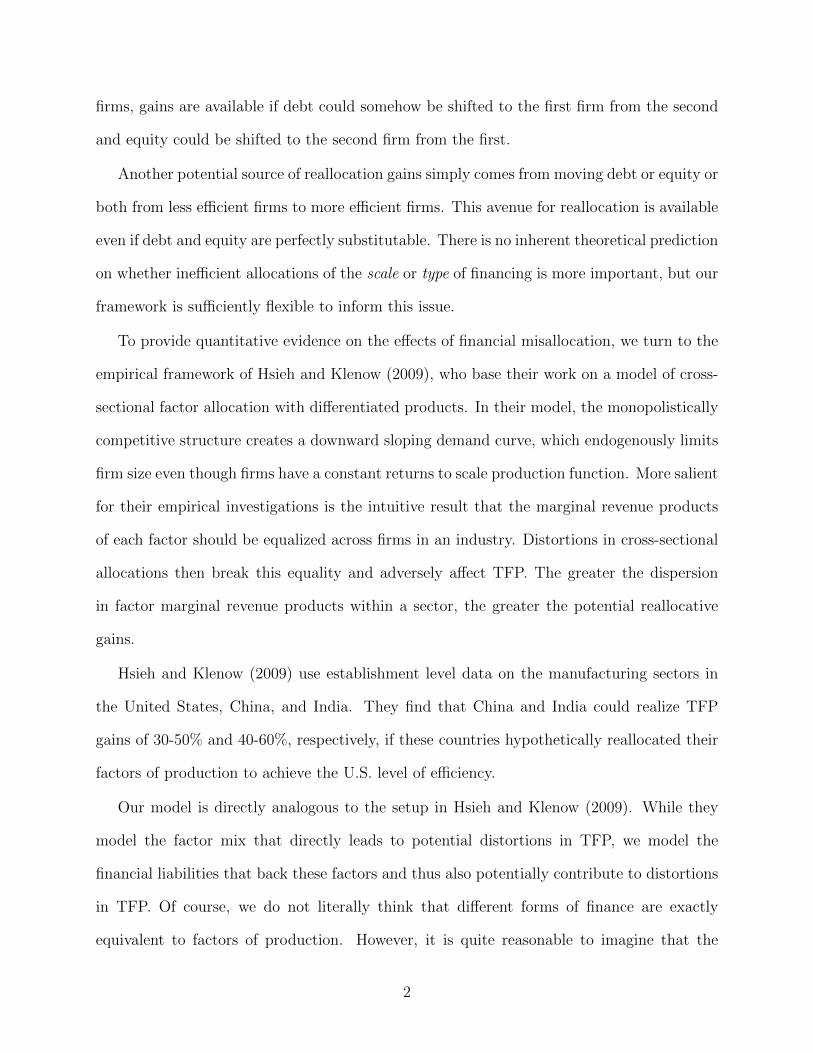
stocks of debt and equity can be aggregated into a measure of benefit to the firm. Moreover,

this aggregation is likely to exhibit decreasing marginal benefits for each different type of

finance. Any model that derives an optimal interior solution for capital structure would lead

to this type of structure.

In our framework, at an optimal allocation, the marginal benefits of debt and equity

finance to total factor benefit should be equal across firms in a sector, and distortions in these

allocations lower productivity. Given this observation, we infer distortions as deviations from

the first best which is derived from first-order conditions for optimal allocations. Empirically,

these deviations manifest themselves as large differences (relative to our model) in the debt-

equity ratio across firms in a sector, and these large differences imply poorly developed

financial markets and large gains from reallocation.

Using U.S. and Chinese data on manufacturing firms, we find significant misallocation

of debt and equity. Although financial liabilities appear well-allocated in the United States,

they are not in China. If China’s debt and equity markets were as developed as those in the

United States, 80% gains in real firm value would be available. We are also able to back out

the cost of debt and equity for each firm with our model, and analyze the cross-sectional

patterns. For instance, larger firms and firms located in more developed cities face markedly

lower costs.

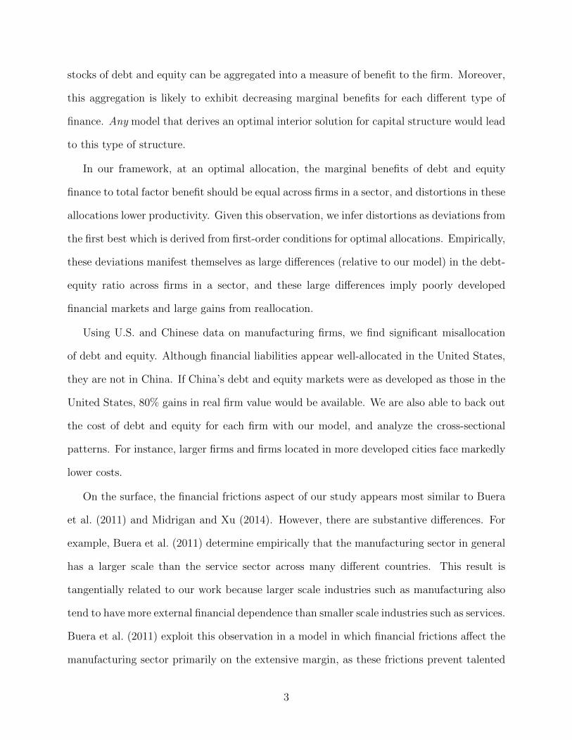
On the surface, the financial frictions aspect of our study appears most similar to Buera

et al. (2011) and Midrigan and Xu (2014). However, there are substantive differences. For

example, Buera et al. (2011) determine empirically that the manufacturing sector in general

has a larger scale than the service sector across many different countries. This result is

tangentially related to our work because larger scale industries such as manufacturing also

tend to have more external financial dependence than smaller scale industries such as services.

Buera et al. (2011) exploit this observation in a model in which financial frictions affect the

manufacturing sector primarily on the extensive margin, as these frictions prevent talented

3

agents from entering this sector. Midrigan and Xu (2014) is also closely related to our

work because they also ask how financial frictions can affect TFP. However, their work is

largely based on a calibrated model, while our work is mostly empirical. In their two sector

model, they find that financial frictions lead to little intensive misallocation but substantial

misallocation across sectors because the more productive sector requires a cost of entry which

is difficult to pay if there are financial frictions.

Like Hsieh and Klenow (2009) and Restuccia and Rogerson (2008), our model has nothing

to say about the extensive margin. The particular type of misallocation we are after comes

from the hypothesis that all forms of finance are not necessarily equivalent. Because we do

recognize that more developed financial markets may cause new firms to enter, our claim is

simply that we provide a lower bound on the extent of capital structure misallocation that

a dynamic model with entry and exit may find.

In the finance literature, our work is related to Graham (2000), who also considers cross-

sectional allocations of debt and equity. However, there are again substantive differences

between our work and his. Graham (2000) computes firm-level estimates of the point at which

the marginal tax benefits of debt begin to decline. A firm that incurs interest deductions

to the left of this “kink” point has an inefficiently low level of debt. Estimates of this

inefficiency imply large amounts of tax benefits left on the table by underleveraged firms:

a puzzle. One notable feature of the framework in Graham (2000) is that he takes relative

prices as given and then interprets deviations from the optimal responses to these prices as

suboptimal behavior. In contrast, we assume that firms behave rationally and then use our

framework to back out the price distortions that lead to the capital structure decisions that

we observe in the data. This alternative perspective seems reasonable in light of the finding

in Blouin, Core, and Guay (2010) that the marginal tax rate estimates of Graham (2000)

imply rational behavior when the kink points are derived from more accurate estimates of

future taxable income.

4

The rest of the paper is organized as follows. Section 2 outlines the model and shows

how the model translates into an empirical framework for measuring misallocation. Section

3 describes the U.S. and Chinese data. Section 4 presents our empirical results, and Section

5 concludes. All proofs are contained in the appendix.

2. Model

Our model closely follows Hsieh and Klenow (2009), which develops a closed-economy version

of Melitz (2003). This section sketches the model, with a description of the environment and

technology, a statement of the optimality conditions, and a description of how to measure

the benefits of reallocation. A full derivation of the model can be found in the appendix.

Environment and technology

Firms in our model are financed by debt and equity. In our model we do not distinguish be-

tween external and internal equity. Given the rarity of seasoned equity offerings (DeAngelo,

DeAngelo, and Stulz 2010), and given that external equity constitutes a negligible source of

funds over the last two decades in the Federal Reserve’s Flow of Funds data, we view this

simplification as innocuous for our purposes.

Firms use the proceeds from these financial assets to generate the real benefit of finance,

and the total real benefit of finance in the economy is denoted by F . We assume that the

economy consists of S sectors, and in each sector s, the real benefit of finance is given by

Fs. These sectoral benefits are are combined using a Cobb-Douglas aggregator, as follows:

F =S∏s=1

F θss , (1)

in which

5

S∑s=1

θs = 1. (2)

The Cobb-Douglas aggregator implies that increasing the size of any particular sector

while holding the others constant has a decreasing marginal benefit.

We next assume that the real benefit of finance Fs for each sector comes from a CES

aggregate of I differentiated firms, as follows:

Fs =

(I∑i=1

Fσ−1σ

si

) σσ−1

, (3)

in which σ is the elasticity of substitution of the real benefit of finance between firms in a

sector.

Finally, we assume that within an individual firm, debt and equity finance can be ag-

gregated using a constant elasticity of substitution (CES) function that combines debt and

equity to determine the real benefit of finance:

Fsi = Asi

(αsD

γ−1γ

si + (1− αs)Eγ−1γ

si

) γγ−1

. (4)

In (4), Asi represents financial total factor benefit (TFB), αs ∈ (0, 1) provides the weight

on the importance of debt in generating this benefit, and γ is the elasticity of substitu-

tion between debt and equity. It is worth noting that using a CES aggregator represents

an important departure from Hsieh and Klenow (2009), who use a Cobb-Douglas produc-

tion function. As will be seen below, the CES aggregator gives us flexibility to distinguish

between reallocation gains that come from the amount of finance and the type. Nonethe-

less, this equation constitutes a strong functional form assumption on how debt and equity

generate a real benefit to the firm. This equation also models the generation of benefits

without explicitly modeling a production function with capital and labor. Implicitly, if firms

6

ultimately finance their purchases of factors of production using debt and equity, then the

proximate factors—capital, materials, labor, and energy—can be thought of as unmodeled

intermediate inputs.

Note that certain variables are firm-specific, while others are sector-specific. For example,

TFB,Asi, depends on both the sector and firm while the weight αs only depends on the sector.

An important feature of the real benefit function is that there is a decreasing marginal benefit

to each individual financial factor input. A functional form with this property suggests a

trade-off model of capital structure. Naturally, (4) also allows for perfect substitutability

between different forms of finance, but even in this case, reallocation gains within a sector

are possible by moving debt or equity from lower TFB firms to higher TFB firms.

Optimal allocations

Next, we define the prices that enter the firm’s optimization problem. First, we let r and λ

be the costs associated with using debt and equity, respectively. Second, to the extent that

financial market frictions distort these costs, we also need to define “taxes” that represent

reduced-form cost distortions. Specifically, τDsi is a “tax” on debt and τEsi is a “tax” on

equity. Positive values indicate that firms face additional costs of finance. As noted in the

introduction, these costs can arise from such frictions as informational asymmetry, agency

problems, or financial sector underdevelopment. Negative values, on the other hand, suggest

favorable financial relationships and/or government subsidies. We do not model the explicit

mechanisms behind the distortions and assume that the they are well-encapsulated by τDsi

and τEsi .

Given these definitions, the nominal net benefit of finance πsi is given by:

πsi = PsiFsi − (1 + τDsi) rDsi − (1 + τEsi)λEsi (5)

Because the right side of (5), (1 + τDsi) rDsi + (1 + τEsi)λEsi, is the cost of capital, πsi can

7

be interpreted as economic value added (EVA), which is a sensible quantity to maximize in a

static model. The one component of (5) that requires more explanation is the interpretation

of Psi. It is somewhat unconventional to specify a price as a choice variable that determines

the nominal benefit of finance, but this feature of our model can be justified as follows. If

a firm has differentiated products, it sets prices in the product market and the benefit of

finance should be related to how well it does on the productive side. Price setting for the

financial side should then be related to price setting for the productive side. In other words,

Psi is the price a differentiated firm would ask for the real benefits it is generating.

An individual firm aims to maximize πsi by choosing Psi, Dsi, and Esi, taking r, λ, τDsi ,

and τEsi as given. To solve the optimization problem, the firm first minimizes the cost of

capital (1 + τDsi) rDsi+(1 + τEsi)λEsi by choosing Dsi and Esi subject to a fixed real benefit

Fsi. Then the firm chooses Psi to maximize the nominal net benefit πsi. The solution to the

firm problem gives:

Psi =σ

σ − 1

1

Asi

((1 + τDsi) r

(αs + (1− αs)Z

− γ−1γ

si

)− γγ−1

+ (1 + τEsi)λ

(αsZ

γ−1γ

si + (1− αs))− γ

γ−1

), (6)

in which

Zsi =

(αs

1− αs(1 + τEsi)λ

(1 + τDsi) r

)γ. (7)

The optimality condition (6) naturally shows that price is a markup over marginal cost.

Next, we solve for the sector price Ps as a function of firm price Psi, by defining Ps to be

the minimum price of acquiring a unit of the sector benefit. The solution is:

8

Ps =

(I∑i=1

P−(σ−1)si

)− 1σ−1

. (8)

Finally, cost minimization of the Cobb-Douglas aggregator across sectors gives:

P =S∏s=1

(Psθs

)θs(9)

in which θs are the weights on each industry, and P is similarly defined to be the minimum

price of acquiring a unit of the aggregate benefit. We assume that the nominal benefit of

finance satisfies value additivity at the sector level and firm level, such that:

S∑s=1

PsFs = PF

andI∑i=1

PsiFsi = PsFs.

From the derivation of P , the industry weights, θs, are found to be the fractions of the

portfolio allocated to each industry, that is:

PsFs = θsPF. (10)

Up to this point, we have made no mention of preferences. Although preferences are

not modeled explicitly, the implicit preferences that produce the results above are CES

preferences over the benefit from firms in a sector and Cobb-Douglas preferences over the

benefit from sectors in the economy.

Reallocation

We now demonstrate how to calculate the gains from reallocation using this framework. To

find the reallocation gains, we first note that we can express financial total factor benefit,

9

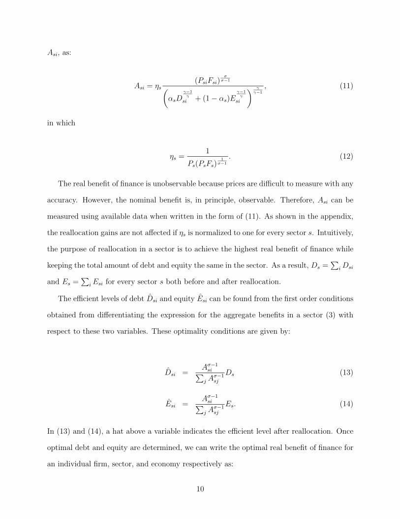
Asi, as:

Asi = ηs(PsiFsi)

σσ−1(

αsDγ−1γ

si + (1− αs)Eγ−1γ

si

) γγ−1

, (11)

in which

ηs =1

Ps(PsFs)1

σ−1

. (12)

The real benefit of finance is unobservable because prices are difficult to measure with any

accuracy. However, the nominal benefit is, in principle, observable. Therefore, Asi can be

measured using available data when written in the form of (11). As shown in the appendix,

the reallocation gains are not affected if ηs is normalized to one for every sector s. Intuitively,

the purpose of reallocation in a sector is to achieve the highest real benefit of finance while

keeping the total amount of debt and equity the same in the sector. As a result, Ds =∑

iDsi

and Es =∑

iEsi for every sector s both before and after reallocation.

The efficient levels of debt Dsi and equity Esi can be found from the first order conditions

obtained from differentiating the expression for the aggregate benefits in a sector (3) with

respect to these two variables. These optimality conditions are given by:

Dsi =Aσ−1si∑

j Aσ−1sj

Ds (13)

Esi =Aσ−1si∑

j Aσ−1sj

Es. (14)

In (13) and (14), a hat above a variable indicates the efficient level after reallocation. Once

optimal debt and equity are determined, we can write the optimal real benefit of finance for

an individual firm, sector, and economy respectively as:

10

Fsi = Asi

(αsD

γ−1γ

si + (1− αs)Eγ−1γ

si

) γγ−1

(15)

Fs =

(∑i

Fσ−1σ

si

) σσ−1

(16)

F =∏s

F θss . (17)

The original, prior to reallocation, real benefit of finance can be computed by replacing

Dsi and Esi by the original debt Dsi and equity Esi in (15) above. Therefore, we can quantify

the gains to reallocation by calculating the observed allocation as a fraction of the efficient

allocation. Letting F denote the observed benefit of finance, these gains are given simply by

F/F .

It is worth discussing the role of the parameters σ and γ in the quantification of these

gains. We first discuss σ, the elasticity of substitution of the real benefit of finance between

firms in a sector. Potential reallocation gains depend positively on σ. To see this point,

consider a case in which firms in a sector are all the same size but their allocations of debt

and equity imply wide dispersion in the benefit of finance, Asi. In this case, moving to the

efficient allocation would result in a great deal of dispersion in firm size, with the much

more productive firms receiving more finance. Thus, overall reallocation gains are greater

when σ is higher. Conversely, a low value for σ implies that reallocating debt and equity

efficiently would result in the most productive firms getting only a modest amount of finance,

so reallocation gains would also be modest.

Turning to γ, the elasticity of substitution between debt and equity, it is intuitive to see

that when γ approaches infinity, debt and equity are perfect substitutes, so the potential

gains from changing the debt-equity mix are zero.

We close this section by showing how to compute the price distortions, τDsi and τEsi . In

11

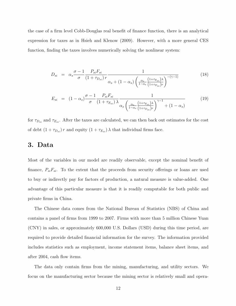
the case of a firm level Cobb-Douglas real benefit of finance function, there is an analytical

expression for taxes as in Hsieh and Klenow (2009). However, with a more general CES

function, finding the taxes involves numerically solving the nonlinear system:

Dsi = αsσ − 1

σ

PsiFsi(1 + τDsi) r

1

αs + (1− αs)(

αs1−αs

(1+τEsi)λ(1+τDsi)r

)−(γ−1)(18)

Esi = (1− αs)σ − 1

σ

PsiFsi(1 + τEsi)λ

1

αs

(αs

1−αs(1+τEsi)λ(1+τDsi)r

)γ−1

+ (1− αs)(19)

for τDsi and τEsi . After the taxes are calculated, we can then back out estimates for the cost

of debt (1 + τDsi) r and equity (1 + τEsi)λ that individual firms face.

3. Data

Most of the variables in our model are readily observable, except the nominal benefit of

finance, PsiFsi. To the extent that the proceeds from security offerings or loans are used

to buy or indirectly pay for factors of production, a natural measure is value-added. One

advantage of this particular measure is that it is readily computable for both public and

private firms in China.

The Chinese data comes from the National Bureau of Statistics (NBS) of China and

contains a panel of firms from 1999 to 2007. Firms with more than 5 million Chinese Yuan

(CNY) in sales, or approximately 600,000 U.S. Dollars (USD) during this time period, are

required to provide detailed financial information for the survey. The information provided

includes statistics such as employment, income statement items, balance sheet items, and

after 2004, cash flow items.

The data only contain firms from the mining, manufacturing, and utility sectors. We

focus on the manufacturing sector because the mining sector is relatively small and opera-

12

tionally different from manufacturing while the utility sector is highly regulated in China.

In addition, we also remove state-owned and collective corporations, which are also known

as Township and Village Enterprises (TVEs). Each firm-year observation is classified as a

private-corporation operating-year if the total state and collective paid-in capital is less than

50%.2 We drop firms with negative and missing industrial value added, total liabilities, and

shareholders’ equity. We also drop firms with less than 5 million 1999 CNY in sales because

the lack of reporting requirements for this group likely results in significant selection bias and

undersampling. After applying these screens, we are left with 1,318,327 remaining firm-year

observations.

We use industrial added value as our measure of the nominal benefit of finance, PsiFsi,

total liabilities for Dsi, and shareholders’ equity for Esi. This measure of equity is the stock

of book equity and thus external equity finance and retained earnings. These variables are all

directly available in the NBS data. Note that we use total liabilities instead of debt, and the

reason behind this choice is twofold. First, debt is not a separately available data item in the

NBS survey, and second, using total liabilities can offer more robust estimation because there

are almost no firms with zero liabilities. For a CES function without an infinite elasticity of

substitution, the marginal benefit of a factor input is unbounded at zero, and this property

of the CES aggregator would present omitted observation problems in the estimation. These

choices for debt and equity imply that the sum of the two equals total assets.

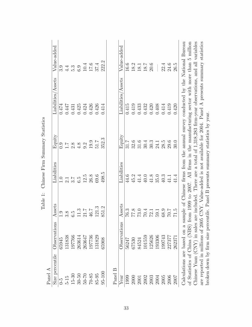
Summary statistics for this sample are in Table 1. Panel A reports various statistics in

the sample stratified by size, where we use a density breakdown of 5%, 10%, 15%, 20%,

20%, 15%, 10%, 5%, so the cumulative density breakdown is 0-5%, 5-15%, 15-30%, 30-50%,

50-70%, 70-85%, 85-95%, 95-100%. This partition is quite attractive because the mean of

total assets roughly doubles for each size group, with the exception of the largest size group,

2This type of classification is often used since official corporate ownership registrations can lag severalyears behind actual ownership changes. For instance, see Guariglia, Liu, and Song (2011) for a similarapproach.

13

which is reflective of the well-known right skewness of the firm size distribution.

In Panel A, we find two patterns in the data of interest. First, the ratio of liabilities to

assets varies little across the different size classes, with the larger firms having only slightly

lower leverage. Second, it is clear from comparing the value-added and assets columns,

that the smaller firms use their assets far more efficiently to produce value-added. This

pattern, juxtaposed with the similarity in leverage across size classes, points strongly to

potential misallocation of capital structure, as firms with different productivities ought to

have different capital structures (Hennessy and Whited 2005).

Panel B presents summary statistics by year. Here, we see that the ratio of liabilities

to assets is little changed over the sample period. Interestingly, the average size of firms

has shrunk somewhat from the beginning to the end of the sample. However, these slightly

smaller firms are creating 60% more value added at the end of the sample than at the

beginning.

For U.S. data, we use Compustat and correspondingly keep only the manufacturing sector

with Standard Industrial Classification (SIC) codes between 2000 and 3999. We also drop

firms with missing and negative data, keep only the years from 1999 to 2007 inclusive.

Value-added is computed in the same manner as in Imrohoroglu and Tuzel (2014). First,

labor costs are estimated from the NBER-CES Manufacturing Industry Database by multi-

plying the number of employees Compustat variable (EMP) by the mean wage per employee

(PAY/EMP) in the firm’s 3-digit SIC industry. Value-added is operating income before de-

preciation (OIBDP) plus the imputed wages. For Dsi and Esi, we use total liabilities and

shareholders’ equity.

We partition the firms by size according to the same densities as before. Of course,

Compustat is a data set of U.S. public firms, so the average firm is much larger. However, the

observed patterns by firm size can still be informative. Table 2 provides summary statistics

by firm size and by year. In Panel A, we again present eight firm size categories, and the last

14

three Chinese firm size categories are approximately equivalent to the first three U.S. firm

size categories. In addition to the results above, we find a hump-shaped relation between

size and leverage for U.S. firms, with the medium-sized firms having the highest leverage.

Also in contrast to the Chinese firms, small and large U.S. firms have approximately the

same ratio of value-added to assets.

Panel B shows two more differences between the Chinese and U.S. firms. First, the U.S.

firms grow from the beginning to the end of our sample. Also, firms become more leveraged

over time.

4. Results

We now use the framework developed in Section 2 to quantify the extent of capital structure

misallocation. Before we present our results, we need to discuss the normalization of several

parameters. First, we set the elasticity of substitution for the real benefit of finance between

firms in an industry to σ = 1.77. Although this choice provides conservative estimates of the

reallocation gains, we also explore below the robustness of our results to this assumption.

Next, the pre-distortion cost of debt and equity is set to r = λ = 0.1. It should be emphasized

that our reallocation results are not sensitive to this normalization because firms only care

about the after tax cost of debt (1 + τDsi) r and equity (1 + τEsi)λ. Changing r and/or λ only

changes the interpretation of the tax distortions relative to the base cost of debt and equity.

The weight on the importance of debt in a sector is set to αs = rD1/γs /(rD

1/γs + λE

1/γs )

which is the value when there are no tax distortions. This assumption is innocuous, as

raising r or λ by 0.05 has a less than 1% impact on the overall reallocation gains. Next,

we set the elasticity of substitution between debt and equity, γ = 2, and again we explore

below the robustness of our results to varying the value of this parameter. Finally, we need

to define sectors. Here, we use 3-digit industry classifications from the Chinese NBS and

3-digit Standard Industrial Classification (SIC) industries from Compustat.

15

Table 3 contains estimates of the potential gains from the reallocation of finance across

firms in a sector. Each row corresponds to a separate year. The first column shows the

observed U.S. allocation of the real benefit of finance as a fraction of the optimal US alloca-

tion: FUS/FUS. The second column shows the corresponding percentage gain from moving

from the observed to the optimal allocation. The next two columns present analogous cal-

culations for Chinese firms. The two columns after that show the Chinese efficiency ratio

as a fraction of the U.S. efficiency ratio: (FChina/FChina)(FUS/FUS), and the corresponding

percentage gains, in other words, the percentage gains available if China’s debt and equity

markets were as developed as those in the United States. The last two columns provide a

breakdown of misallocation into the misallocation due to scale and due to misallocation of

factors, holding scale fixed.

Bootstrapped standard errors are in parentheses under the parameter estimates. All of

the standard errors are quite small. This result makes sense inasmuch as the figures that we

present are all essentially means, which can be estimated with a great deal of precision with

several thousand data points.

In the first two columns, we see that U.S. public firms stand to gain about 13-18% in

moving to an optimal allocation. The potential gains appear to be less during the boom

periods and greater during the recession during the early part of our sample. This result

makes sense inasmuch as financial frictions are generally regarded to be more severe in

recessions. In the next two columns, we see, somewhat surprisingly, the efficiency of the

allocation of debt and equity appears to worsen over our sample period in China. This

phenomenon can be mostly attributed to the expansion of the NBS survey in the 2004

Industrial Census, which picked up firms that were left out in previous annual surveys.3

When we restrict our sample to firms that are in the NBS survey before and after the 2004

Industrial Census, the pattern of increasing misallocation is lessened.

3Brandt, Van Biesebroeck, and Zhang (2014) discuss the impact of the 2004 Industrial Census on theNBS survey sample.

16

The available reallocation gains appear enormous. We find that value-added could poten-

tially be increased by over 100% if the Chinese firms were to move to an efficient allocation.

Although these figures seem large, they are of the same order of magnitude as the estimated

gains found in Hsieh and Klenow (2009) regarding capital and labor allocations.

To put these results in more perspective, we now examine the last four columns in Table 3.

The column labeled “relative fractional benefit” shows the efficiency gains in China relative

to the efficiency gains in the United States. This comparison is motivated by the observation

in Hsieh and Klenow (2009) that because a simple static model based on the framework in

Melitz (2003) is likely to be misspecified, a researcher is likely to observe positive potential

gains even when allocations are efficient. This observation is particularly applicable in our

context of financial misallocation because U.S. financial markets are highly developed. Thus,

by comparing the potential gains in China relative to the observed gains in the United States,

we isolate the potential gains in China relative to an assumed efficient allocation. Here, the

results are more modest. We find potential gains of approximately 70% before the expansion

of the NBS survey, and of approximately 100% after the expansion.

To understand whether these gains come from the amount of finance available to Chinese

firms or to the type of finance, we compare the relative fractional benefit to a case in which

we set γ = ∞. If γ = ∞, then the type of finance does not matter for the aggregate

benefit of finance because debt and equity are perfect substitutes. This exercise produces

an interesting result. We find that the majority of the potential reallocation gains come

from the misallocation of scale. Before the expansion of the NBS survey, we find that only

approximately 8% of the gains could be realized by reallocating the type of finance. After

the expansion, this figure rises to between 11.7% to 14.1%. This result is interesting because

it means that the access to finance in general is behind the large potential TFP losses in

China.

We next examine the robustness of the reallocation results to the calibration of the

17

parameters γ and σ, the elasticity of substitutions between debt and equity and elasticity of

substitution between firms in an industry, respectively. These results are in Table 4. First,

we find that allowing γ to range between 1.5 and 10 has a negligible effect our estimates

of percent gains in both the United States and China. By construction, γ has no effect on

the misallocation of scale. However, changing γ does materially alter our estimates of the

percent of of gains that come from reallocating the type of finance, with lower levels of γ

corresponding to more gains. Thus, our estimates in Table 3 can be thought of as upper

bounds, and this interpretation leaves intact our general qualitative result that the vast

majority of potential gains from the the misallocation of scale.

While varying γ has little effect on our estimated reallocation gains, varying σ does. We

find that the estimated gains increase sharply when we increase σ. Intuitively, the firm size

distribution becomes excessively skewed if σ is too large because, in this case, all resources

flow to the most productive firms. In other words, if one were to pick the most productive

Chinese firms in a sector and give them all the resources, the gains would be large because

of the substantial dispersion in productivity.

However, as we have argued above, the calibration of σ is conservative if σ is chosen to be

on the low end. We now expand on these arguments. One way to discipline the choice of σ is

to calculate the distributions of debt and equity when the allocation is efficient and compare

these distributions to the realized distributions in the data. For the United States, when

σ = 1.77, the standard deviation of the efficient size distribution is exactly the same as the

observed standard deviation, that is, the standard deviation of Dsi+ Esi equals the standard

deviation of Dsi + Esi. We argue that this choice of σ is very conservative, because if σ is

lower, the efficient size distribution would be more compressed than the observed. However,

when σ rises above 2, the efficient size distribution becomes more and more stretched out

and the reallocation gains become quite large.

We now examine the implications of our estimates for the cross-sectional distribution of

18

firm size. Recall that because of downward sloping demand, each firm has a well-defined

optimal size, with an optimal financing mix. Deviations of the financing amount and mix

from the optimal allocation therefore impact firm size, so comparing the distributions of

firm size under the actual and efficient allocations is a useful way to quantify misallocation.

Figure 1 illustrates this idea with plots of the observed and efficient firm size distributions for

the United States and China. We compute observed firm size as log(Dsi +Esi) and efficient

firm size as log(Dsi+Esi). Panel A shows that the efficient U.S. firm size distribution exhibits

approximately as much dispersion as the actual distribution. Of course, this result is to be

expected, given our calibration of σ. Nonetheless, we do observe somewhat less dispersion in

the actual distribution than in the efficient distribution, especially in the left tail. This result

points to inefficient quantities of financing for the smallest U.S. firms. In contrast, in Panel

B, we see that the efficient firm size distribution for China has a significantly fatter left tail,

with far too few small Chinese firms. These size distortions in turn stem from misallocation

of either the amount or mix of financing to the affected firms.

Although the plots in Figure 1 show the firm size distributions before and after realloca-

tion, they do not illustrate the individual changes in firm size that happens with reallocation.

Figure 2 shows these movements via heat maps. Panel A contains the heat map of a three-

dimensional histogram in which the observed U.S. firm size distribution is on the x-axis and

the efficient U.S. firm size distribution is on the y-axis. The legend for the z-axis heat map is

located at right of the map and represents the number of observations in each bin. Similarly,

Panel B contains the heat map for China. From the heat maps, we can see that U.S. firms

are concentrated along the 45 degree line, where firm size before and after reallocation is

the same. In contrast, Chinese firms are much more spread out, reflecting the substantial

efficiency gains available from reallocation. Interestingly, both heat maps are more concen-

trated towards the top right than towards the bottom left. This pattern indicates that small

firms are more likely to suffer from financial misallocation than large firms.

19

Next, we move on to the distortions in the prices of debt and equity that we can back

out of our estimation. Table 5 summarizes the post-distortion cost of debt (1 + τDsi) r and

equity (1 + τEsi)λ by year, again under the assumptions that γ = 2 and σ = 1.77. Panel A

contains means and Panel B contains medians. In Panel A, we find that the costs of debt

and equity fall over the sample period in the United States. In contrast, these costs rise in

China over the same time period. This pattern reinforces the result in Table 3 that points

to greater misallocation after 2004, when the NBS survey samples more firms. These extra

firms exhibit more misallocation and consequently greater costs of debt and equity. Finally,

the figures in Panel B are uniformly much smaller than those in Panel A, especially for the

Chinese firms. This result points to extreme right skewness in the distribution of the cost of

finance, implying that some firms are likely effectively barred from financial markets.

Table 6 is structured exactly as Table 5, except the sample is stratified by size instead

of year. In the United States, the average cost of debt is substantially lower for large firms,

while the cost of equity displays no clear pattern across firm size. This second result is

consistent with the well-documented lack of a size premium in equity markets in recent

years. In contrast, both the costs of debt and equity are dramatically lower for large Chinese

firms in comparison to small Chinese firms.

Beyond analyzing the cost of debt and equity by year and firm size, we run two descriptive

OLS regressions on our sample of Chinese firms to examine how these costs vary by firm

characteristics. Specifically, we regress the cost of debt and equity respectively on location,

state investment, firm size, time, and firm age. Location is a dummy variable that equals 1 if

a firm is located in Beijing, Shanghai, Shenzhen, or Guangzhou and 0 otherwise. These four

Chinese cities are also known as first tier cities and are the most developed in China. State

investment is a dummy variable that equals 1 if a firm has a non-zero percentage of paid-in-

capital from state sources and 0 otherwise. However, note that all firms in our sample are

private. The dummy variable just indicates whether there is any state investment. Next,

20

size is the log of total assets measured in 2005 CNY. Finally, time is a simple linear time

trend, and age is firm age in years and is censored at 100 years.

Table 7 presents the results. We find that costs are significantly lower for larger firms,

and this result confirms our cross-sectional sorts by size in Table 6. Firms operating in first

tier Chinese cities also face lower costs. Surprisingly, firms with non-zero state investment

actually face slightly higher costs on average. It is important to note that this result is

conditional on firm size. If we break down the total set of firms into those with and without

state paid-in-capital, we find that firms with state paid-in-capital have lower costs. However,

these firms are also significantly larger, so the effect of state investment on costs reverses once

we control for size. Next, the positive coefficient on the time trend reflects the increasing

costs also evident in Table 5. Finally, firm age is associated with a statistically significant

but tiny decrease in the cost of debt, as well as a tiny increase in the cost of equity.

Table 8 offers another robustness check of the model. In all of our work thus far, we have

measured the nominal benefit of finance using value-added. A natural alternative measure

is the sum of the market values of debt and equity. Of course, we cannot use this measure

in our sample of Chinese firms, as most of these firms are not publicly traded. However, we

look at the measure in our sample of U.S. firms. We find that overall reallocation gains are

similar in magnitude to those in Table 3. One exception can be found during the dot-com

boom, in which we find more misallocation.

5. Conclusion

This paper entertains the possibility that finance may be misallocated in the cross-section

of firms. We explore this hypothesis using a tractable model of differentiated firms based

on Hsieh and Klenow (2009). In our framework, the optimal allocation of debt and equity

equates the marginal benefit of these two securities within an industry. Thus, observed

dispersion in the marginal benefit of debt and marginal benefit of equity is symptomatic of

21

misallocation.

Our evidence points only to modest potential reallocation gains in the United States,

with American firms standing to gain only 13-18% in terms of aggregate real firm value if

they were to move to an efficient allocation. Our results are much more dramatic for China,

where firms stand to gain over 100% from moving to the efficient allocation. If China was

able to achieve the more reasonable U.S. level of efficiency, gains of 70-100% would still be

possible. When we break this figure down by the amount versus the type of finance, we find

that nearly all of this figure can be attributed to the amount of finance and little to the mix

of securities used to fund a firm’s operations.

Our work sheds light on the interaction between productive and financial allocation and

the puzzling persistence of productive misallocation. Here, Banerjee and Moll (2010) show

in a model that productive misallocation along the intensive margin should disappear within

several years. Yet Hsieh and Klenow (2009) show that this type of misallocation has not

dissipated over time. The financial misallocation we investigate in this paper may be related

to productive misallocation and can help explain this puzzle. For instance, debt financing

might be more conducive to capital investment, and if financial frictions are persistent, the

misallocation of productive factors should be as well. Overall, we believe that productivity

losses can result both from the misallocation of debt and equity and from the misallocation

of capital and labor. We leave to further work for an analysis of these forms of misallocation

together in a unified framework.

22

Appendix

Aggregate price

We begin by solving for the aggregate price P as a function of sector price Ps, where P is de-

fined to be the minimum price of acquiring a unit of the aggregate benefit. The minimization

problem is mathematically stated as:

minFs

{∑s

PsFs

}, (20)

subject to:

∏s

F θss = F . (21)

The Lagrangian is:

L = −∑s

PsFs +M

[∏s

F θss − F

], (22)

where M is the Lagrange multiplier. The first-order condition with respect to Fs gives:

Ps = Mθs

∏s F

θss

Fs, (23)

which simplifies to:

PsFsθs

= PF (24)

because M = P . After aggregation of sectors in the economy, we can write the aggregate

price as a function of sector price:

23

P =∏s

(Psθs

)θs. (25)

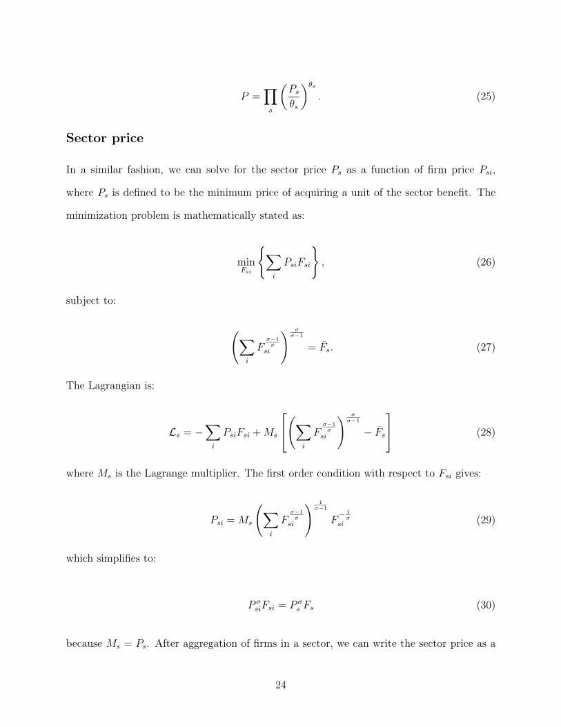
Sector price

In a similar fashion, we can solve for the sector price Ps as a function of firm price Psi,

where Ps is defined to be the minimum price of acquiring a unit of the sector benefit. The

minimization problem is mathematically stated as:

minFsi

{∑i

PsiFsi

}, (26)

subject to:

(∑i

Fσ−1σ

si

) σσ−1

= Fs. (27)

The Lagrangian is:

Ls = −∑i

PsiFsi +Ms

(∑i

Fσ−1σ

si

) σσ−1

− Fs

(28)

where Ms is the Lagrange multiplier. The first order condition with respect to Fsi gives:

Psi = Ms

(∑i

Fσ−1σ

si

) 1σ−1

F− 1σ

si (29)

which simplifies to:

P σsiFsi = P σ

s Fs (30)

because Ms = Ps. After aggregation of firms in a sector, we can write the sector price as a

24

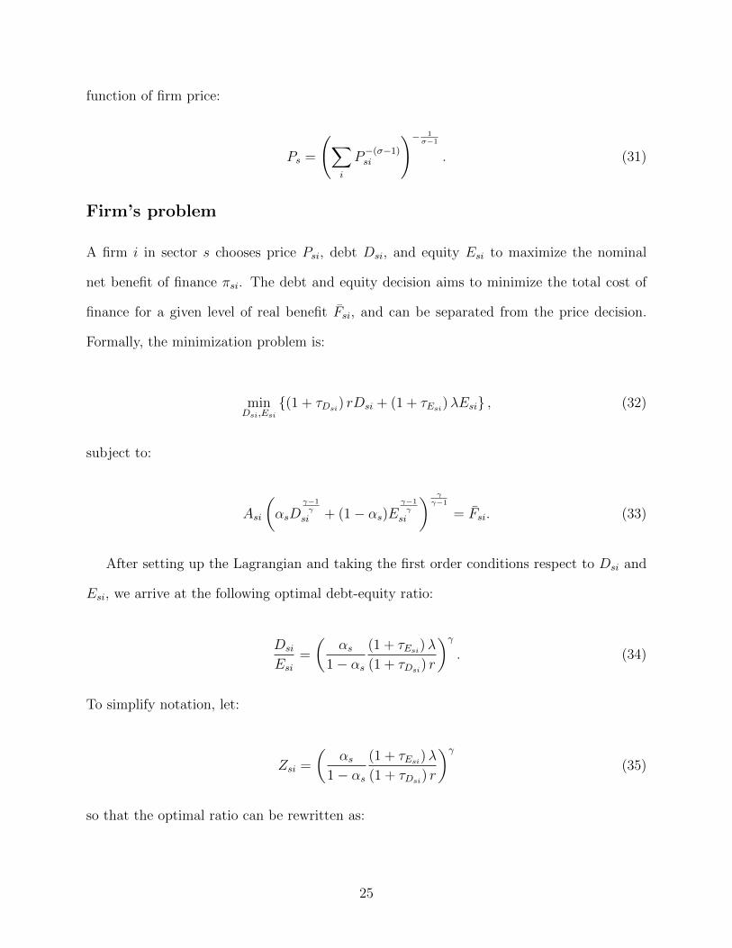
function of firm price:

Ps =

(∑i

P−(σ−1)si

)− 1σ−1

. (31)

Firm’s problem

A firm i in sector s chooses price Psi, debt Dsi, and equity Esi to maximize the nominal

net benefit of finance πsi. The debt and equity decision aims to minimize the total cost of

finance for a given level of real benefit Fsi, and can be separated from the price decision.

Formally, the minimization problem is:

minDsi,Esi

{(1 + τDsi) rDsi + (1 + τEsi)λEsi} , (32)

subject to:

Asi

(αsD

γ−1γ

si + (1− αs)Eγ−1γ

si

) γγ−1

= Fsi. (33)

After setting up the Lagrangian and taking the first order conditions respect to Dsi and

Esi, we arrive at the following optimal debt-equity ratio:

Dsi

Esi=

(αs

1− αs(1 + τEsi)λ

(1 + τDsi) r

)γ. (34)

To simplify notation, let:

Zsi =

(αs

1− αs(1 + τEsi)λ

(1 + τDsi) r

)γ(35)

so that the optimal ratio can be rewritten as:

25

Dsi

Esi= Zsi. (36)

Debt and equity can thus be expressed as linear functions of the real benefit, as follows:

Dsi =FsiAsi

(αs + (1− αs)Z

− γ−1γ

si

)− γγ−1

Esi =FsiAsi

(αsZ

γ−1γ

si + (1− αs))− γ

γ−1

(37)

Then using the above expressions for debt and equity, the minimum cost function becomes

a function of the fixed real benefit Fsi:

C(Fsi) = (1 + τDsi) rDsi + (1 + τEsi)λEsi

= CsiFsi,(38)

where

Csi =1

Asi

((1 + τDsi) r

(αs + (1− αs)Z

− γ−1γ

si

)− γγ−1

+ (1 + τEsi)λ

(αsZ

γ−1γ

si + (1− αs))− γ

γ−1

).

(39)

Next, we choose Psi to maximize the nominal net benefit of finance, that is:

maxPsi{πsi} = max

Psi{PsiFsi − CsiFsi} . (40)

Recall from the sector price derivation that firm real benefit is a function of sector price,

firm price, and sector real benefit, Fsi =(PsPsi

)σFs. Therefore, the firm’s real benefit is just

a function of price once the optimal debt-equity ratio is computed, and the firm faces a

downward sloping demand curve. The maximization problem is bounded due to downward

sloping demand even though the firm has constant returns to scale. From the first order

26

condition on price we find:

Psi =σ

σ − 1Csi. (41)

Note that the price is a fixed markup over marginal cost and a higher elasticity of substitution

between firms in a sector lowers the price the firm can charge for the real benefit it is

generating.

Taxes

To solve for the tax distortions, the nominal benefit of finance should first be written as:

PsiFsi = PsF1σs F

σ−1σ

si . (42)

The marginal nominal benefit of debt must equal the marginal nominal cost of debt for

the maximizing firm, so the first order condition with respect to Dsi gives:

PsF1σsσ − 1

σF

− 1σ

si Asi

(αsD

γ−1γ

si + (1− αs)Eγ−1γ

si

) γγ−1

−1

αsD− 1γ

si = (1 + τDsi) r (43)

which simplifies to:

Dsi = αsσ − 1

σ

PsiFsi(1 + τDsi) r

1

αs + (1− αs)(

αs1−αs

(1+τEsi)λ(1+τDsi)r

)−(γ−1). (44)

Similarly, the first order condition with respect to Esi simplifies to:

Esi = (1− αs)σ − 1

σ

PsiFsi(1 + τEsi)λ

1

αs

(αs

1−αs(1+τEsi)λ(1+τDsi)r

)γ−1

+ (1− αs). (45)

The taxes for each firm can be backed out by solving the nonlinear system of two equations

27

(44) and (45) and two unknowns τDsi and τEsi .

Efficient allocation

We now turn to the derivation of the efficient allocation in a sector. Under the efficient

allocation, total debt and total equity in a sector are kept the same, but debt and equity are

reallocated across firms in a sector to maximize sector real benefit. The debt-equity ratio

Zsi = DsEs

= Zs can be shown to be the same for all firms i in sector s when debt and equity

are reallocated to achieve efficiency. The real benefit of finance can then be written as a

function of Dsi:

Fsi =

(αs + (1− αs)Z

− γ−1γ

s

) γγ−1

AsiDsi, (46)

where a hat above a variable indicates the efficient level after reallocation. The Lagrangian

is:

Ls =

∑i

((αs + (1− αs)Z

− γ−1γ

s

) γγ−1

AsiDsi

)σ−1σ

σσ−1

+ Ms

[∑i

Dsi −Ds

](47)

where Ms is the Lagrange multiplier. The first order condition with respect to Dsi and Dsj

for firms i and j respectively rearranges to:

(Dsi

Dsj

)− 1σ

=

(AsjAsi

)σ−1σ

. (48)

After aggregation, the expression above can be simplified to:

Dsi =Aσ−1si∑

j Aσ−1sj

Ds. (49)

The optimal equity allocation can be similarly derived as:

28

Esi =Aσ−1si∑

j Aσ−1sj

Es. (50)

The real benefit Fsi is assumed to be unobservable. However, Asi can be expressed as

variables obtainable from data such as the nominal benefit PsiFsi, that is:

Asi = ηs(PsiFsi)

σσ−1(

αsDγ−1γ

si + (1− αs)Eγ−1γ

si

) γγ−1

(51)

where

ηs =1

Ps(PsFs)1

σ−1

(52)

because

FsiPs(PsFs)1

σ−1 = (PsiFsi)σσ−1 . (53)

Reallocation gains are not affected if ηs is normalized to one for all sectors s.

Aggregation

The ultimate goal is to find the ratio of the aggregate real benefit computed from data over

the efficient allocation. The real benefit computed from data is given by:

Fsi = Asi

(αsD

γ−1γ

si + (1− αs)Eγ−1γ

si

) γγ−1

Fs =

(∑i

Fσ−1σ

si

) σσ−1

F =∏s

F θss ,

(54)

29

while the efficient allocation is given by:

Fsi = Asi

(αsD

γ−1γ

si + (1− αs)Eγ−1γ

si

) γγ−1

Fs =

(∑i

Fσ−1σ

si

) σσ−1

F =∏s

F θss .

(55)

Therefore, the ratio is F/F .

30

References

Alfaro, Laura, Andrew Charlton, and Fabio Kanczuk, 2009, Plant-size distribution and cross-country income differences, in Jeffrey A. Frankel, and Christopher Pissarides: eds., NBERInternational Seminar on Macroeconomics (National Bureau of Economic Research, Cam-bridge, MA).

Banerjee, Abhijit V., and Esther Duflo, 2005, Growth theory through the lens of develop-ment economics, in Philippe Aghion, and Steven N. Durlauf: eds., Handbook of EconomicGrowth, volume 1A, chapter 7, 473–552 (Elsevier).

Banerjee, Abhijit V., and Benjamin Moll, 2010, Why does misallocation persist?, AmericanEconomic Journal: Macroeconomics 2, 189–206.

Bartelsman, Eric, John Haltiwanger, and Stefano Scarpetta, 2013, Cross-country differencesin productivity: The role of allocation and selection, American Economic Review 103,305–334.

Blouin, Jennifer, John E. Core, and Wayne Guay, 2010, Have the tax benefits of debt beenoverestimated?, Journal of Financial Economics 98, 195–213.

Brandt, Loren, Johannes Van Biesebroeck, and Yifan Zhang, 2014, Challenges of workingwith the chinese nbs firm-level data, China Economic Review 30, 339–352.

Buera, Francisco J., Joseph P. Kaboski, and Yongseok Shin, 2011, Finance and development:A tale of two sectors, American Economic Review 101, 1964–2002.

Chen, Kaiji, and Zheng Song, 2013, Financial frictions on capital allocation: A transmissionmechanism of tfp fluctuations, Journal of Monetary Economics 60, 683–703.

Cooley, Thomas F., and Vincenzo Quadrini, 2001, Financial markets and firm dynamics,American Economic Review 91, 1286–1310.

DeAngelo, Harry, Linda DeAngelo, and Rene M. Stulz, 2010, Seasoned equity offerings,market timing, and the corporate lifecycle, Journal of Financial Economics 95, 275–295.

Graham, John R., 2000, How big are the tax benefits of debt?, Journal of Finance 55,1901–1941.

Guariglia, Alessandra, Xiaoxuan Liu, and Lina Song, 2011, Internal finance and growth:Microeconometric evidence on chinese firms, Journal of Development Economics 96, 79–94.

Hennessy, Christopher A., and Toni M. Whited, 2005, Debt dynamics, Journal of Finance60, 1129–1165.

Hopenhayn, Hugo, and Richard Rogerson, 1993, Job turnover and policy evaluation: Ageneral equilibrium analysis, Journal of Political Economy 101, 915–938.

Hopenhayn, Hugo A., 1992, Entry, exit, and firm dynamics in long run equilibrium, Econo-metrica 60, 1127–1150.

31

Hsieh, Chang-Tai, and Peter J. Klenow, 2009, Misallocation and manufacturing tfp in chinaand india, Quarterly Journal of Economics 124, 1403–1448.

Hsieh, Chang-Tai, and Peter J. Klenow, 2014, The life cycle of plants in india and mexico,Quarterly Journal of Economics 129, 1035–1084.

Imrohoroglu, Ayse, and Selale Tuzel, 2014, Firm-level productivity, risk, and return, Man-agement Science 60, 2073–2090.

Jeong, Hyeok, and Robert M. Townsend, 2007, Sources of tfp growth: occupational choiceand financial deepening, Economic Theory 32, 179–221.

Melitz, Marc J., 2003, The impact of trade on intra-industry reallocations and aggregateindustry productivity, Econometrica 71, 1695–1725.

Midrigan, Virgiliu, and Daniel Yi Xu, 2014, Finance and misallocation: Evidence fromplant-level data, American Economic Review 104, 422–458.

Olley, G. Steven, and Ariel Pakes, 1996, The dynamics of productivity in the telecommuni-cations equipment industry, Econometrica 64, 1263–1297.

Petrin, Amil, and James Levinsohn, 2012, Measuring aggregate productivity growth usingplant-level data, RAND Journal of Economics 43, 705–725.

Restuccia, Diego, and Richard Rogerson, 2008, Policy distortions and aggregate productivitywith heterogeneous establishments, Review of Economic Dynamics 11, 707–720.

Robert E. Lucas, Jr., 1978, On the size distribution of business firms, Bell Journal of Eco-nomics 9, 508–523.

Song, Zheng, Kjetil Storesletten, and Fabrizio Zilibotti, 2011, Growing like China, AmericanEconomic Review 101, 196–233.

Syverson, Chad, 2011, What determines productivity?, Journal of Economic Literature 49,326–365.

32

Tab

le1:

Chin

ese

Fir

mSum

mar

ySta

tist

ics

Pan

elA

Siz

ep

erce

nti

leO

bse

rvat

ions

Ass

ets

Lia

bilit

ies

Equit

yL

iabilit

ies/

Ass

ets

Val

ue-

added

0-5

6594

51.

91.

00.

90.

474

3.9

5-15

1318

383.

82.

11.

70.

447

4.4

15-3

019

7766

6.5

3.7

2.8

0.43

15.

330

-50

2636

1411

.36.

54.

80.

425

6.9

50-7

026

3647

21.7

12.5

9.2

0.42

410

.470

-85

1977

3646

.726

.819

.90.

426

17.6

85-9

513

1829

121.

369

.651

.70.

426

37.4

95-1

0065

908

851.

249

8.5

352.

30.

414

222.

2

Pan

elB

Yea

rO

bse

rvat

ions

Ass

ets

Lia

bilit

ies

Equit

yL

iabilit

ies/

Ass

ets

Val

ue-

added

1999

5624

776

.344

.631

.70.

415

16.6

2000

6753

077

.845

.232

.60.

419

18.2

2001

8452

473

.041

.431

.60.

433

18.1

2002

1015

5970

.440

.030

.40.

432

18.7

2003

1256

2672

.141

.830

.30.

420

20.6

2004

1933

0659

.135

.024

.10.

408

—–

2005

1997

4368

.940

.328

.50.

414

22.4

2006

2273

7770

.741

.129

.60.

419

24.6

2007

2623

7171

.541

.430

.00.

420

26.5

Cal

cula

tion

sar

ebas

edon

asa

mple

ofC

hin

ese

firm

sfr

omth

ean

nual

surv

eyco

nduct

edby

the

Nat

ional

Bure

auof

Sta

tist

ics

ofC

hin

a(N

BS)

from

1999

to20

07.

All

firm

sin

the

man

ufa

cturi

ng

sect

orw

ith

mor

eth

an5

million

Chin

ese

Yuan

(CN

Y)

insa

les

are

incl

uded

.T

her

ear

ea

tota

lof

1,31

8,28

3firm

-yea

rob

serv

atio

ns,

and

all

vari

able

sar

ere

por

ted

inm

illion

sof

2005

CN

Y.

Val

ue-

added

isnot

avai

lable

for

2004

.P

anel

Apre

sents

sum

mar

yst

atis

tics

bro

ken

dow

nby

firm

size

per

centi

le.

Pan

elB

pre

sents

sum

mar

yst

atis

tics

by

year

.

33

Tab

le2:

U.S

.F

irm

Sum

mar

ySta

tist

ics

Pan

elA

Siz

ep

erce

nti

leO

bse

rvat

ions

Ass

ets

Lia

bilit

ies

Equit

yL

iabilit

ies/

Ass

ets

Val

ue-

added

0-5

1005

7.8

3.6

4.2

0.53

80.

45-

1520

0220

.88.

912

.00.

574

4.7

15-3

030

0351

.720

.131

.60.

611

12.4

30-5

040

0014

0.0

52.4

87.6

0.62

641

.550

-70

4005

464.

421

3.0

251.

60.

542

158.

570

-85

3003

1583

.287

5.3

708.

20.

447

545.

985

-95

2002

6114

.336

21.6

2492

.70.

408

1996

.695

-100

996

4203

7.1

2450

3.8

1753

3.4

0.41

711

957.

2

Pan

elB

Yea

rO

bse

rvat

ions

Ass

ets

Lia

bilit

ies

Equit

yL

iabilit

ies/

Ass

ets

Val

ue-

added

1999

2589

2126

.712

84.4

846.

20.

397

651.

720

0025

5224

09.8

1408

.210

06.2

0.41

778

1.6

2001

2392

2461

.014

37.9

1027

.50.

417

742.

020

0222

4427

30.7

1629

.111

07.9

0.40

579

3.1

2003

2121

3240

.819

04.3

1340

.90.

413

912.

220

0421

0734

60.1

1982

.314

81.7

0.42

810

36.4

2005

2058

3643

.620

80.6

1569

.70.

430

1103

.720

0620

1839

72.5

2231

.217

52.1

0.44

011

74.1

2007

1935

4206

.223

17.9

1900

.20.

450

1199

.2

Cal

cula

tion

sar

ebas

edon

asa

mple

ofm

anufa

cturi

ng

firm

s(S

IC20

00to

3999

)fr

omC

ompust

at.

The

sam

ple

per

iod

is19

99to

2007

and

incl

udes

20,0

16firm

-yea

rob

serv

atio

ns.

All

vari

able

sar

ere

por

ted

inm

illion

sof

2005

USD

.V

alue-

added

isop

erat

ing

inco

me

bef

ore

dep

reci

atio

n(O

IBD

P)

plu

sim

pute

dw

ages

.Im

pute

dw

ages

are

calc

ula

ted

by

mult

iply

ing

the

emplo

ym

ent

ofea

chfirm

wit

hth

em

ean

wag

ep

erem

plo

yee

inth

eap

pro

pri

ate

3-dig

itSIC

indust

ry.

Pan

elA

pre

sents

sum

mar

yst

atis

tics

bro

ken

dow

nby

firm

size

per

centi

le.

Pan

elB

pre

sents

sum

mar

yst

atis

tics

by

year

.

34

Tab

le3:

Rea

lloca

tion

Gai

ns

by

Yea

r

Un

ited

Sta

tes

Ch

ina

Un

ited

Sta

tes

vs.

Ch

ina

Yea

rF

ract

ion

alb

enefi

tP

erce

nt

Gai

nF

ract

ion

al

ben

efit

Per

cent

Gain

Rel

ati

vefr

act

ion

al

ben

efit

Per

cent

Gain

Per

cent

Sca

leP

erce

nt

Fact

or

1999

0.87

114

.80.4

93

102.9

0.5

66

76.7

67.5

9.1

(0.0

12)

(1.5

)(0

.008)

(3.4

)(0

.012)

(3.8

)(3

.4)

(0.7

)20

000.

856

16.9

0.4

95

101.9

0.5

79

72.8

65.0

7.8

(0.0

14)

(1.8

)(0

.008)

(3.0

)(0

.012)

(3.7

)(3

.3)

(0.6

)20

010.

863

15.9

0.5

06

97.6

0.5

87

70.5

62.4

8.0

(0.0

15)

(2.0

)(0

.008)

(2.9

)(0

.014)

(4.1

)(3

.8)

(0.5

)20

020.

850

17.7

0.5

08

97.0

0.5

97

67.4

59.9

7.6

(0.0

19)

(2.5

)(0

.008)

(2.9

)(0

.016)

(4.6

)(4

.2)

(0.6

)20

030.

847

18.1

0.5

03

98.7

0.5

94

68.3

60.7

7.6

(0.0

17)

(2.2

)(0

.005)

(2.1

)(0

.012)

(3.5

)(3

.3)

(0.5

)20

040.

860

16.2

—–

—–

—–

—–

—–

—–

(0.0

15)

(2.0

)20

050.

878

13.9

0.4

46

124.1

0.5

08

96.8

85.1

11.7

(0.0

13)

(1.7

)(0

.007)

(3.3

)(0

.011)

(4.3

)(3

.8)

(0.7

)20

060.

876

14.2

0.4

41

126.7

0.5

04

98.6

86.2

12.4

(0.0

11)

(1.4

)(0

.005)

(2.5

)(0

.007)

(3.0

)(2

.6)

(0.6

)20

070.

888

12.6

0.4

29

133.2

0.4

83

107.2

93.1

14.1

(0.0

09)

(1.1

)(0

.004)

(2.4

)(0

.007)

(3.2

)(2

.8)

(0.7

)

Cal

cula

tion

sar

eb

ased

ontw

osa

mp

les

offi

rms.

On

esa

mp

leco

nst

itu

tes

U.S

.fi

rms

from

Com

pust

at,

an

dth

eoth

erco

nst

itu

tes

asa

mp

leof

Ch

ines

efi

rms

from

the

Nat

ion

alB

ure

au

of

Sta

tist

ics

of

Ch

ina.

Th

esa

mp

lep

erio

dis

from

1999

to20

07

incl

usi

ve.

Valu

e-ad

ded

isn

otav

aila

ble

in20

04fo

rC

hin

ese

firm

s.T

his

tab

lep

rese

nts

pote

nti

al

reall

oca

tion

gain

sw

hen

the

sub

stit

uta

bil

ity

bet

wee

nd

ebt

an

deq

uit

yisγ

=2.

Th

efi

rst

colu

mn

show

sth

eob

serv

edU

.S.

all

oca

tion

of

the

real

ben

efit

of

fin

an

ceas

afr

act

ion

of

the

op

tim

al

US

allo

cati

on:FUS/FUS.

Th

ese

con

dco

lum

nsh

ows

the

corr

esp

on

din

gp

erce

nta

ge

gain

from

mov

ing

from

the

ob

serv

edto

the

op

tim

al

allo

cati

on.

Th

en

ext

two

colu

mn

sp

rese

nt

an

alo

gou

sca

lcu

lati

on

sfo

rC

hin

ese

firm

s.T

he

two

colu

mn

saft

erth

at

show

the

Ch

ines

eeffi

cien

cyra

tio

asa

frac

tion

ofth

eU

.S.

effici

ency

rati

o:

(FChina/F

China)(FUS/FUS),

an

dth

eco

rres

pon

din

gp

erce

nta

ge

gain

s,in

oth

erw

ord

s,th

ep

erce

nta

gega

ins

avai

lab

leif

Ch

ina’s

deb

tan

deq

uit

ym

ark

ets

wer

eas

dev

elop

edas

those

inth

eU

nit

edS

tate

s.T

he

last

two

colu

mn

sp

rovid

ea

bre

akd

own

ofm

isall

oca

tion

into

the

mis

all

oca

tion

du

eto

scale

an

dd

ue

tom

isall

oca

tion

of

fact

ors

,h

old

ing

scal

efi

xed

.B

elow

each

esti

mat

e,th

eco

rres

pon

din

gst

an

dard

erro

ris

rep

ort

edin

pare

nth

eses

.

35

Tab

le4:

Rea

lloca

tion

Gai

ns

by

Ela

stic

itie

sof

Subst

ituti

on

Unit

edSta

tes

Chin

aU

nit

edSta

tes

vs.

Chin

a

Yea

rF

ract

ional

ben

efit

Per

cent

Gai

nF

ract

ional

ben

efit

Per

cent

Gai

n

Rel

ativ

efr

acti

onal

ben

efit

Per

cent

Gai

nP

erce

nt

Sca

leP

erce

nt

Fac

tor

γ=

1.5

0.85

816

.50.

461

116.

80.

537

86.1

71.6

14.5

γ=

20.

865

15.6

0.47

810

9.3

0.55

281

.171

.69.

5γ

=3

0.87

214

.70.

492

103.

20.

564

77.2

71.6

5.6

γ=

50.

877

14.0

0.50

299

.10.

572

74.7

71.6

3.1

γ=

100.

881

13.5

0.50

996

.40.

578

73.0

71.6

1.4

σ=

1.5

0.88

413

.10.

541

84.9

0.61

263

.455

.67.

8σ

=1.

770.

865

15.6

0.47

810

9.3

0.55

281

.171

.69.

5σ

=2

0.84

917

.70.

425

135.

10.

501

99.7

88.3

11.4

σ=

2.5

0.81

422

.90.

321

211.

30.

395

153.

413

6.3

17.1

σ=

30.

778

28.5

0.24

031

7.5

0.30

822

4.9

200.

124

.8

Cal

cula

tion

sar

ebas

edon

two

sam

ple

sof

firm

s.O

ne

sam

ple

const

itute

sU

.S.

firm

sfr

omC

ompust

at,

and

the

other

const

itute

sa

sam

ple

ofC

hin

ese

firm

sfr

omth

eN

atio

nal

Bure

auof

Sta

tist

ics

ofC

hin

a.T

he

sam

ple

per

iod

isfr

om19

99to

2007

incl

usi

ve.

Val

ue-

added

isnot

avai

lable

in20

04fo

rC

hin

ese

firm

s.T

his

table

pre

sents

pot

enti

alre

allo

cati

onga

ins

aver

aged

acro

ssal

lye

ars

when

we

allo

wth

eel

asti

citi

esof

subst

ituti

on,γ

andσ

,to

vary

.W

hen

γis

vari

ed,σ

isse

tto

1.77

,an

dw

hen

σis

vari

ed,γ

isse

tto

2.T

he

firs

tco

lum

nsh

ows

the

obse

rved

U.S

.al

loca

tion

ofth

ere

alb

enefi

tof

finan

ceas

afr

acti

onof

the

opti

mal

US

allo

cati

on:FUS/F

US.

The

seco

nd

colu

mn

show

sth

eco

rres

pon

din

gp

erce

nta

gega

infr

omm

ovin

gfr

omth

eob

serv

edto

the

opti

mal

allo

cati

on.

The

nex

ttw

oco

lum

ns

pre

sent

anal

ogou

sca

lcula

tion

sfo

rC

hin

ese

firm

s.T

he

two

colu

mns

afte

rth

atsh

owth

eC

hin

ese

effici

ency

rati

oas

afr

acti

onof

the

U.S

.effi

cien

cyra

tio:

(FChina/F

China)(FUS/F

US),

and

the

corr

esp

ondin

gp

erce

nta

gega

ins,

inot

her

wor

ds,

the

per

centa

gega

ins

avai

lable

ifC

hin

a’s

deb

tan

deq

uit

ym

arke

tsw

ere

asdev

elop

edas

thos

ein

the

Unit

edSta

tes.

The

last

two

colu

mns

pro

vid

ea

bre

akdow

nof

mis

allo

cati

onin

toth

em

isal

loca

tion

due

tosc

ale

and

due

tom

isal

loca

tion

offa

ctor

s,hol

din

gsc

ale

fixed

.

36

Table 5: Costs of Debt and Equity by Year

Panel A: United States China

Year (1 + τDsi) r (1 + τEsi)λ (1 + τDsi) r (1 + τEsi)λ

1999 0.219 0.182 0.307 0.281(0.0034) (0.0070) (0.0035) (0.0029)

2000 0.217 0.183 0.314 0.289(0.0044) (0.0034) (0.0044) (0.0023)

2001 0.202 0.167 0.322 0.301(0.0042) (0.0034) (0.0035) (0.0023)

2002 0.206 0.172 0.334 0.313(0.0038) (0.0043) (0.0030) (0.0018)

2003 0.209 0.179 0.403 0.321(0.0048) (0.0114) (0.0057) (0.0017)

2004 0.210 0.171 —– —–(0.0041) (0.0033)

2005 0.209 0.174 0.448 0.366(0.0042) (0.0035) (0.0037) (0.0022)

2006 0.206 0.170 0.491 0.390(0.0042) (0.0037) (0.0049) (0.0016)

2007 0.197 0.165 0.579 0.443(0.0051) (0.0043) (0.0041) (0.0024)

Panel B: United States China

Year (1 + τDsi) r (1 + τEsi)λ (1 + τDsi) r (1 + τEsi)λ

1999 0.181 0.154 0.146 0.158(0.0029) (0.0021) (0.0008) (0.0008)

2000 0.178 0.156 0.153 0.167(0.0029) (0.0023) (0.0007) (0.0008)

2001 0.162 0.139 0.163 0.175(0.0024) (0.0024) (0.0008) (0.0007)

2002 0.167 0.141 0.171 0.182(0.0030) (0.0024) (0.0006) (0.0008)

2003 0.162 0.136 0.179 0.188(0.0031) (0.0023) (0.0006) (0.0006)

2004 0.167 0.140 —– —–(0.0027) (0.0023)

2005 0.171 0.143 0.196 0.201(0.0027) (0.0026) (0.0005) (0.0005)

2006 0.164 0.142 0.209 0.215(0.0041) (0.0019) (0.0006) (0.0006)

2007 0.156 0.132 0.230 0.236(0.0032) (0.0021) (0.0006) (0.0006)

This table displays the estimated mean (Panel A) and median (Panel B)costs of debt (1 + τDsi) r and equity (1 + τEsi)λ in the US and Chinaby year. The elasticity of substitution between debt and equity is set atγ = 2. Below each estimate, the corresponding standard error is reportedin parentheses.

37

Table 6: Costs of Debt and Equity by Firm Size

Panel A: United States China

Percentile (1 + τDsi) r (1 + τEsi)λ (1 + τDsi) r (1 + τEsi)λ

0-5 0.313 0.205 1.666 1.109(0.0163) (0.0108) (0.0237) (0.0095)

5-15 0.279 0.201 0.762 0.606(0.0087) (0.0062) (0.0054) (0.0036)

15-30 0.243 0.186 0.556 0.451(0.0049) (0.0040) (0.0043) (0.0015)

30-50 0.239 0.173 0.401 0.346(0.0034) (0.0049) (0.0025) (0.0013)

50-70 0.203 0.170 0.310 0.274(0.0024) (0.0042) (0.0022) (0.0012)

70-85 0.167 0.171 0.238 0.217(0.0017) (0.0024) (0.0016) (0.0014)

85-95 0.150 0.165 0.180 0.173(0.0018) (0.0021) (0.0016) (0.0011)

95-100 0.133 0.138 0.150 0.143(0.0018) (0.0019) (0.0097) (0.0010)

Panel B: United States China

Percentile (1 + τDsi) r (1 + τEsi)λ (1 + τDsi) r (1 + τEsi)λ

0-5 0.253 0.161 0.746 0.641(0.0073) (0.0050) (0.0041) (0.0027)

5-15 0.214 0.155 0.385 0.385(0.0052) (0.0024) (0.0013) (0.0011)

15-30 0.197 0.143 0.268 0.282(0.0029) (0.0024) (0.0006) (0.0007)

30-50 0.201 0.137 0.198 0.213(0.0027) (0.0018) (0.0005) (0.0005)

50-70 0.171 0.140 0.158 0.166(0.0018) (0.0018) (0.0004) (0.0004)

70-85 0.155 0.148 0.130 0.134(0.0020) (0.0018) (0.0003) (0.0003)

85-95 0.139 0.149 0.111 0.114(0.0016) (0.0020) (0.0004) (0.0004)

95-100 0.122 0.128 0.097 0.101(0.0017) (0.0017) (0.0005) (0.0004)

This table displays the estimated mean (Panel A) and median (Panel B) costsof debt (1 + τDsi) r and equity (1 + τEsi)λ in the US and China by firm size.Firm size is defined to be the 0-5%, 5-15%, 15-30%, 30-50%, 50-70%, 70-85%,85-95%, 95-100% total asset percentiles of firms in each country. The elasticityof substitution between debt and equity is set at γ = 2. Below each estimate,the corresponding standard error is reported in parentheses.

38

Table 7: The Costs of Debt and Equity and Firm Characteristics

(1 + τDsi) r (1 + τEsi)λLocation -0.134 -0.092

(-26.7) (-39.2)State investment 0.055 0.013

(7.8) (4.0)Size -0.192 -0.132

(-153.3) (-225.9)Time 0.032 0.018

(47.7) (56.7)Age -0.001 0.001

(-3.8) (8.1)

This table summarizes two OLS regressions on the costs ofdebt (1 + τDsi) r and equity (1 + τEsi)λ respectively. The re-gressors are location, state investment, firm size, time, andfirm age. Location is a dummy variable that equals 1 if afirm is located in Beijing, Shanghai, Shenzhen, or Guangzhouand 0 otherwise. State investment is a dummy variable thatequals 1 if a firm has a non-zero percentage of paid-in-capitalfrom state sources and 0 otherwise. Size is log total assetsmeasured in 2005 CNY. Time is a linear time trend, andage is firm age in years, which is censored at 100 years. Be-low each estimate, the corresponding t-statistic is reported inparentheses.

39

Table 8: U.S. Reallocation Gains with Market Value Benefit

United StatesYear Fractional benefit Percent Gain

1999 0.740 35.2(0.026) (4.6)

2000 0.746 34.1(0.029) (5.1)

2001 0.854 17.1(0.012) (1.6)

2002 0.889 12.4(0.011) (1.3)

2003 0.890 12.4(0.010) (1.2)

2004 0.890 12.3(0.010) (1.2)

2005 0.887 12.8(0.010) (1.2)

2006 0.891 12.2(0.008) (1.0)

2007 0.865 15.6(0.013) (1.7)

Calculations are based on U.S. firms from Compustat. The sample period isfrom 1999 to 2007 inclusive. The nominal benefit of finance is measured asthe market value of debt plus the market value of equity, instead of value-added. This table presents potential reallocation gains when the substitutabilitybetween debt and equity is γ = 2. The first column shows the observed U.S.allocation of the real benefit of finance as a fraction of the optimal US allocation:FUS/FUS. The second column shows the corresponding percentage gain frommoving from the observed to the optimal allocation. Below each estimate, thecorresponding standard error is reported in parentheses.

40

Panel A:

Log size0 2 4 6 8 10 12

Den

sity

0

0.02

0.04

0.06

0.08

0.1

0.12

0.14

0.16

0.18U.S. firm size distribution

ObservedEfficient

Panel B:

Log size-2 -1 0 1 2 3 4 5 6 7 8

Den

sity

0

0.05

0.1

0.15

0.2

0.25

0.3

0.35China firm size distribution

ObservedEfficient

Figure 1: Panel A compares the U.S. observed and efficient firm size distributions using akernel density estimator. Observed firm size is computed as log(Dsi+Esi), and efficient firmsize is computed as log(Dsi + Esi), where Dsi, Esi, Dsi, and Esi are measured in millions of2005 USD. Panel B similarly compares the observed and efficient firm size distributions inChina. Firm size is computed in the same manner, but Dsi, Esi, Dsi, and Esi are measuredin millions of 2005 CNY.

41

Panel A:

Panel B:

Figure 2: Panel A contains the heat map of a 3D histogram where the observed U.S. firmsize distribution is on the x-axis and the efficient U.S. firm size distribution is on the y-axis.The legend for the z-axis heat map is located at right of the plot and represents the numberof observations in each bin. Observed firm size is computed as log(Dsi + Esi), and efficientfirm size is computed as log(Dsi+ Esi), where Dsi, Esi, Dsi, and Esi are measured in millionsof 2005 USD. Panel B similarly compares the observed and efficient firm size distributions inChina. Firm size is computed in the same manner, but Dsi, Esi, Dsi, and Esi are measuredin millions of 2005 CNY.

42