the modelling of rare events - isaac newton institute · the modelling of rare events: ... 31. jan....
TRANSCRIPT

The Modelling of Rare Events: from methodology to practice and back
Paul Embrechts Department of Mathematics
RiskLab, ETH Zurich
www.math.ethz.ch/~embrechts
The menu (8 take-homes):
• Some EVT history
• Risk measures
• The Pickands – Balkema – de Haan Theorem
• An example: CIs and profile likelihood
• Karamata slow/regular variation
• Rates of convergence in EVT
• An example: micro correlation
• Communication
• Discussion and final example

1713 - 2013
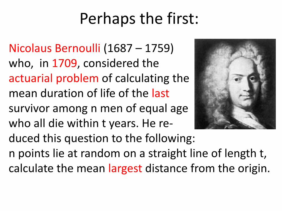
Perhaps the first:
Nicolaus Bernoulli (1687 – 1759) who, in 1709, considered the actuarial problem of calculating the mean duration of life of the last survivor among n men of equal age who all die within t years. He re- duced this question to the following: n points lie at random on a straight line of length t, calculate the mean largest distance from the origin.
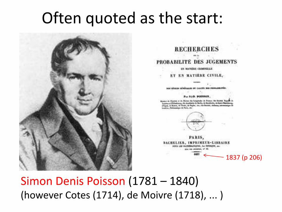
Often quoted as the start:
Simon Denis Poisson (1781 – 1840) (however Cotes (1714), de Moivre (1718), ... )
1837 (p 206)
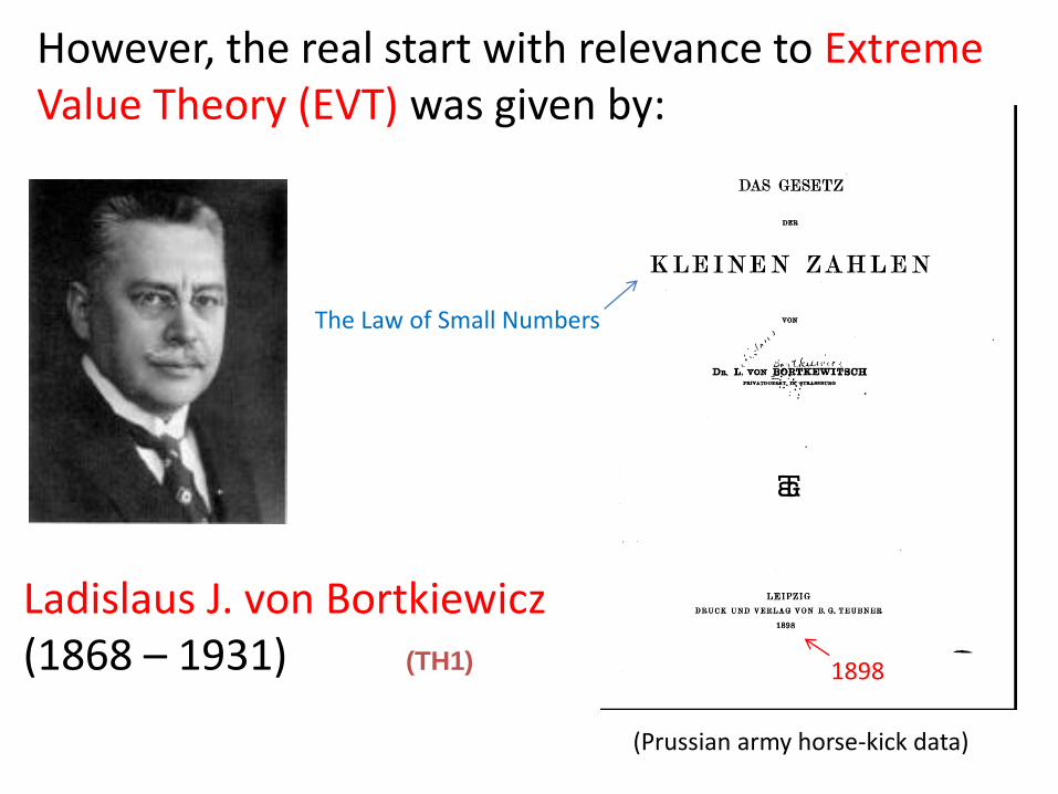
Ladislaus J. von Bortkiewicz (1868 – 1931)
However, the real start with relevance to Extreme Value Theory (EVT) was given by:
The Law of Small Numbers
1898
(Prussian army horse-kick data)
(TH1)

Then came numerous developments in the early to mid 20th century with
famous names like ...
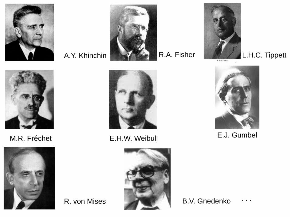
R.A. Fisher L.H.C. Tippett
M.R. Fréchet E.H.W. Weibull E.J. Gumbel
B.V. Gnedenko . . . R. von Mises
A.Y. Khinchin
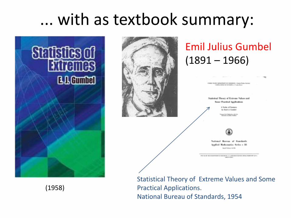
... with as textbook summary:
(1958)
Emil Julius Gumbel (1891 – 1966)
Statistical Theory of Extreme Values and Some Practical Applications. National Bureau of Standards, 1954

The later-20th Century, some names:
Laurens de Haan Sidney I. Resnick
Richard L. Smith M. Ross Leadbetter
and so many more ...
o o o
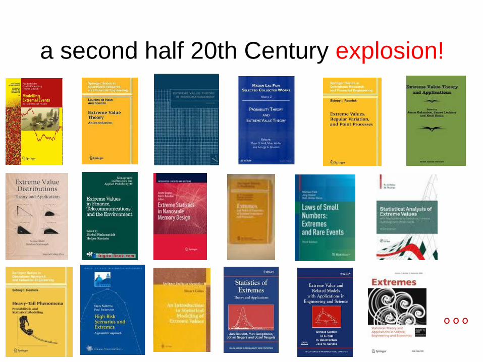
a second half 20th Century explosion!
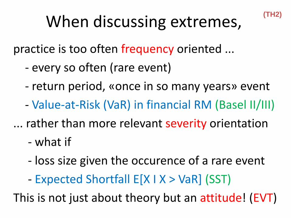
When discussing extremes,
practice is too often frequency oriented ...
- every so often (rare event)
- return period, «once in so many years» event
- Value-at-Risk (VaR) in financial RM (Basel II/III)
... rather than more relevant severity orientation
- what if
- loss size given the occurence of a rare event
- Expected Shortfall E[X I X > VaR] (SST)
This is not just about theory but an attitude! (EVT)
(TH2)
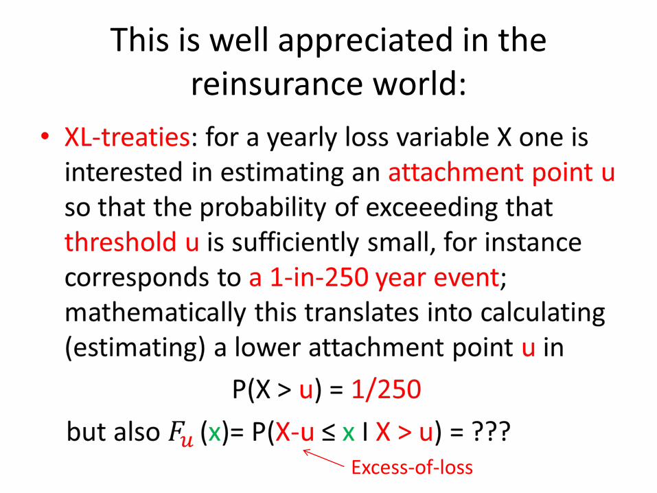
This is well appreciated in the reinsurance world:
Excess-of-loss
This leads to «The Pickands-Balkema-de Haan Theorem», sometimes quoted as
the most important mathematical result for reinsurance!
(Gary Patrick, an American reinsurance actuary)
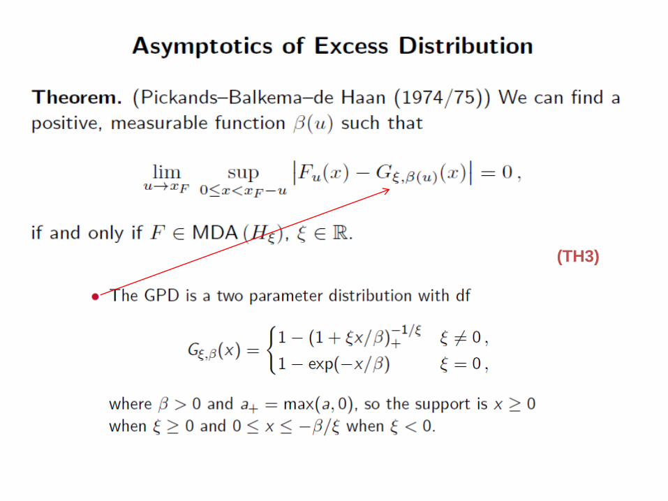
(TH3)
For details and applications, see
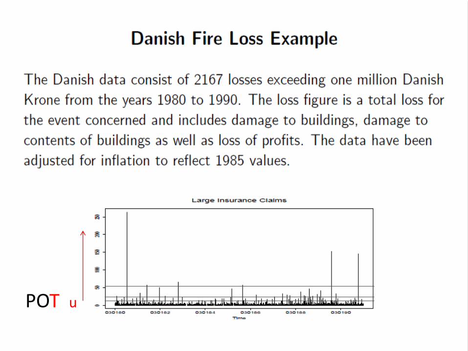
POT u
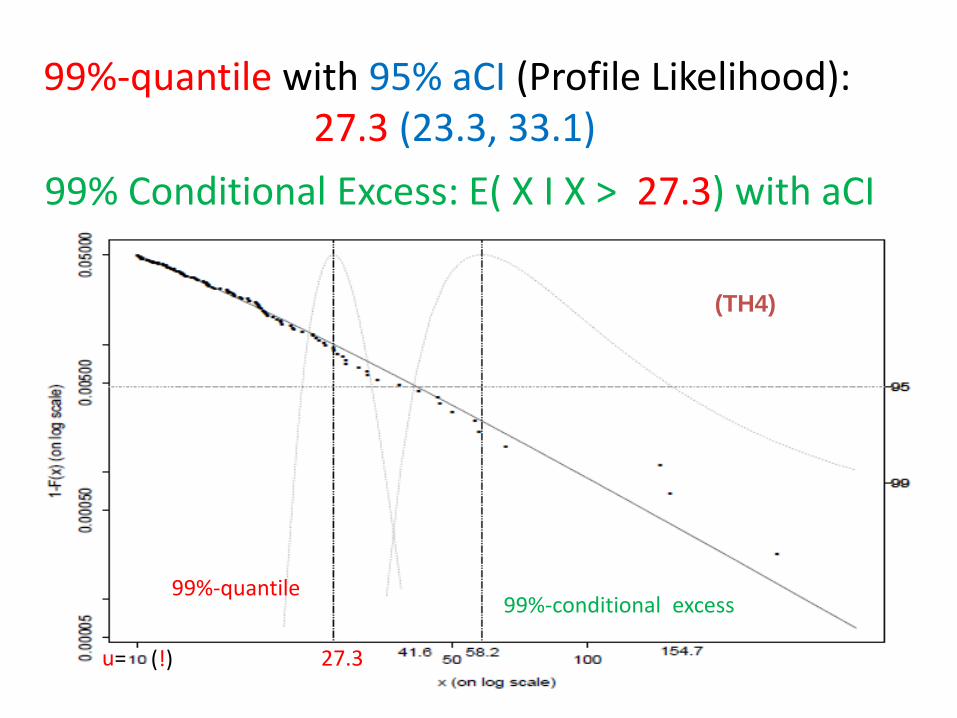
99%-quantile 99%-conditional excess
99%-quantile with 95% aCI (Profile Likelihood): 27.3 (23.3, 33.1)
99% Conditional Excess: E( X I X > 27.3) with aCI
27.3 u= (!)
(TH4)
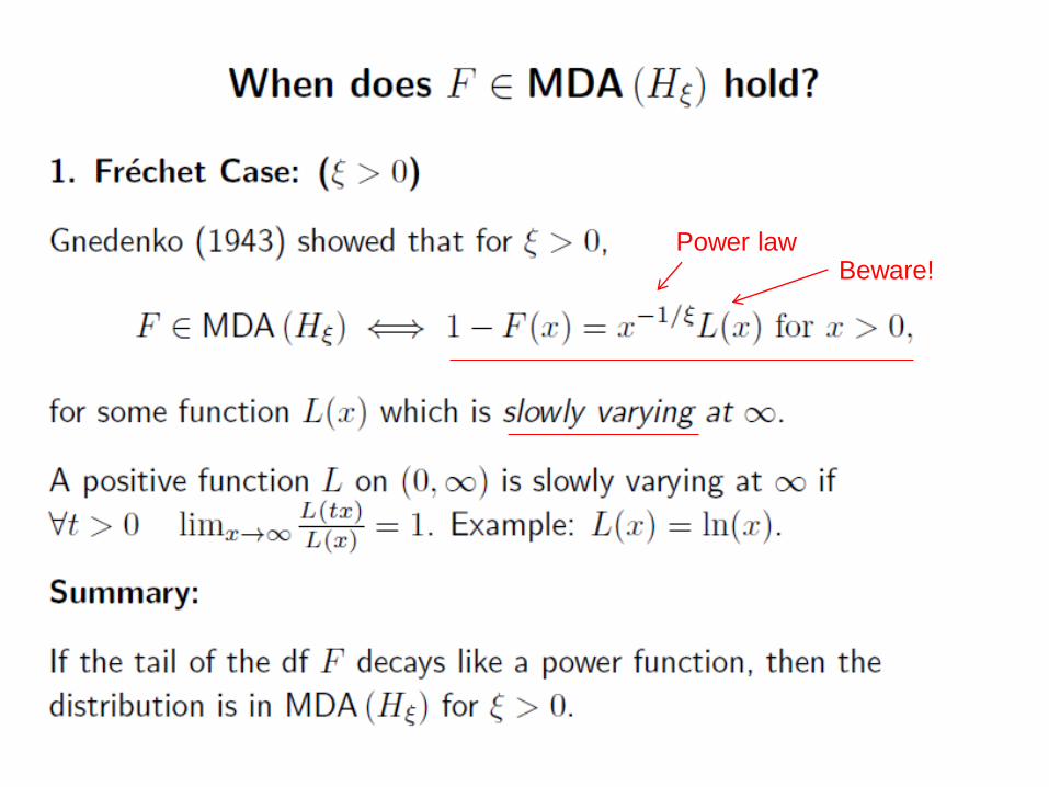
Power law Beware!
An interludium on Regular Variation, more in particular, on the Slowly
Varying L in Gnedenko’s Theorem:
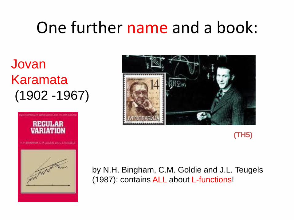
One further name and a book:
Jovan
Karamata
(1902 -1967)
by N.H. Bingham, C.M. Goldie and J.L. Teugels
(1987): contains ALL about L-functions!
(TH5)
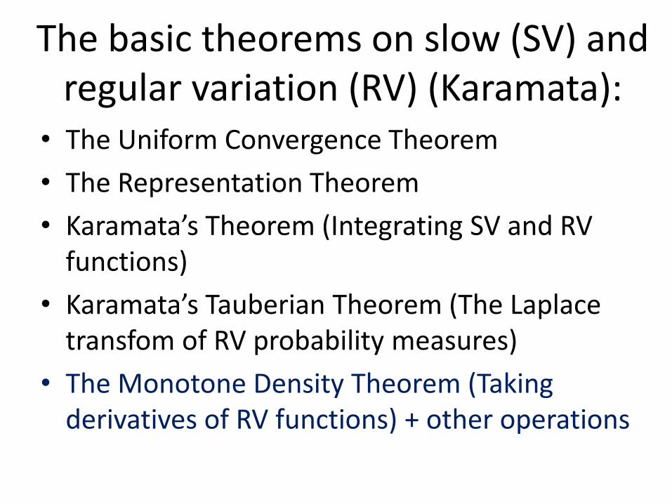
The basic theorems on slow (SV) and regular variation (RV) (Karamata):
• The Uniform Convergence Theorem
• The Representation Theorem
• Karamata’s Theorem (Integrating SV and RV functions)
• Karamata’s Tauberian Theorem (The Laplace transfom of RV probability measures)
• The Monotone Density Theorem (Taking derivatives of RV functions) + other operations
A warning on EVT related rates of convergence:
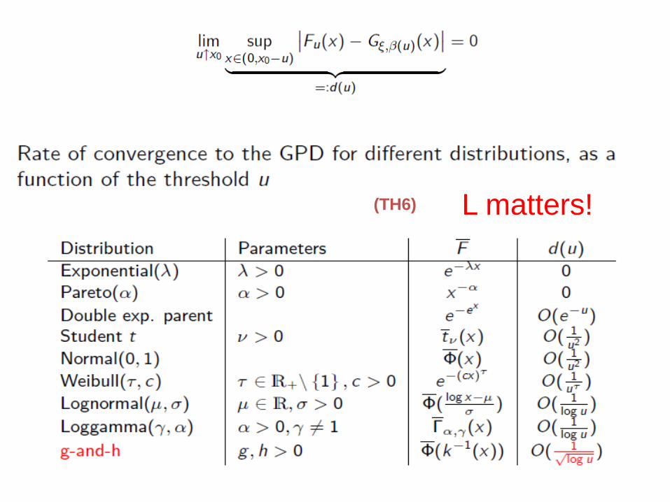
L matters! (TH6)
A warning on micro-correlation and extreme-tail modelling:
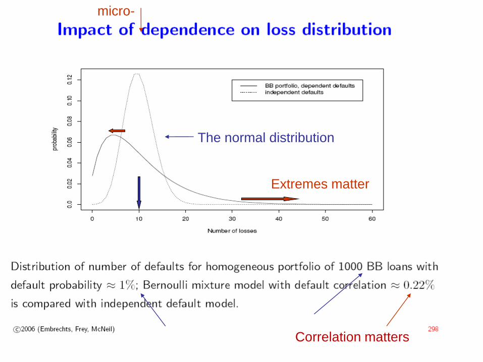
The normal distribution
Extremes matter
Correlation matters
micro-
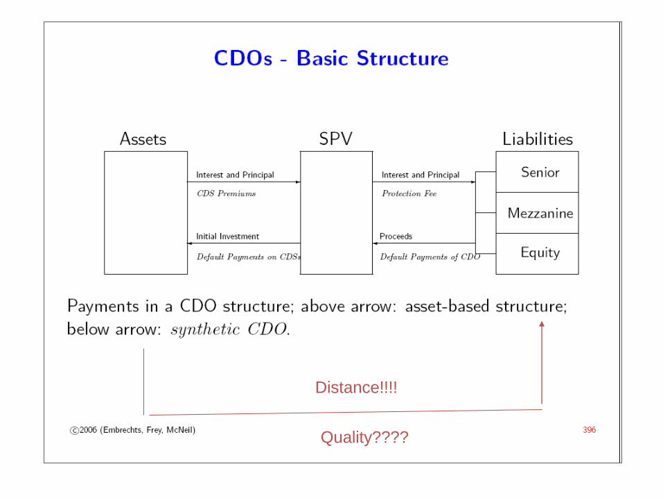
Distance!!!!
Quality????
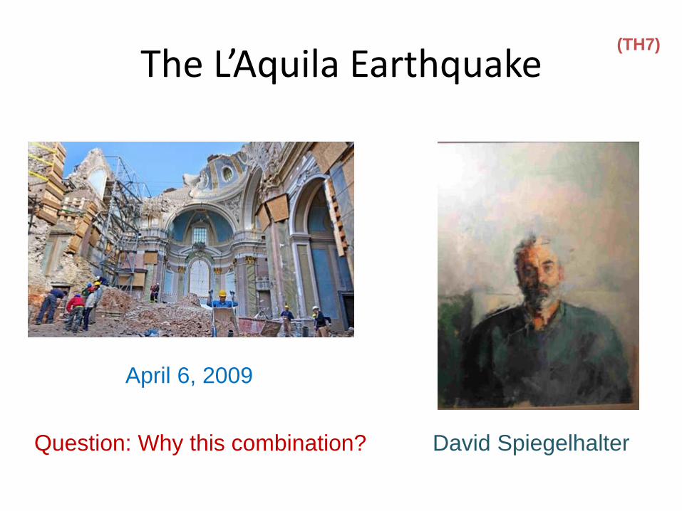
The L’Aquila Earthquake
April 6, 2009
David Spiegelhalter Question: Why this combination?
(TH7)
A final example:
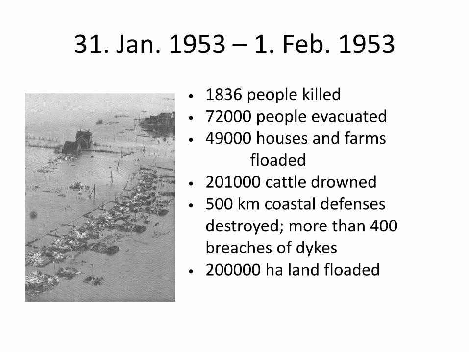
31. Jan. 1953 – 1. Feb. 1953
• 1836 people killed • 72000 people evacuated • 49000 houses and farms floaded • 201000 cattle drowned • 500 km coastal defenses
destroyed; more than 400 breaches of dykes
• 200000 ha land floaded
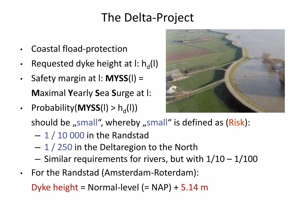
The Delta-Project
• Coastal fload-protection
• Requested dyke height at l: hd(l)
• Safety margin at l: MYSS(l) =
Maximal Yearly Sea Surge at l:
• Probability(MYSS(l) > hd(l))
should be „small“, whereby „small“ is defined as (Risk):
– 1 / 10 000 in the Randstad – 1 / 250 in the Deltaregion to the North – Similar requirements for rivers, but with 1/10 – 1/100
• For the Randstad (Amsterdam-Roterdam):
Dyke height = Normal-level (= NAP) + 5.14 m
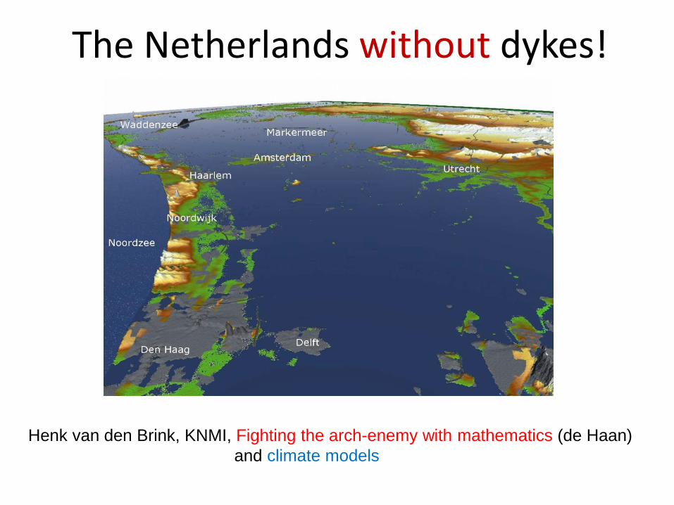
The Netherlands without dykes!
Henk van den Brink, KNMI, Fighting the arch-enemy with mathematics (de Haan)
and climate models
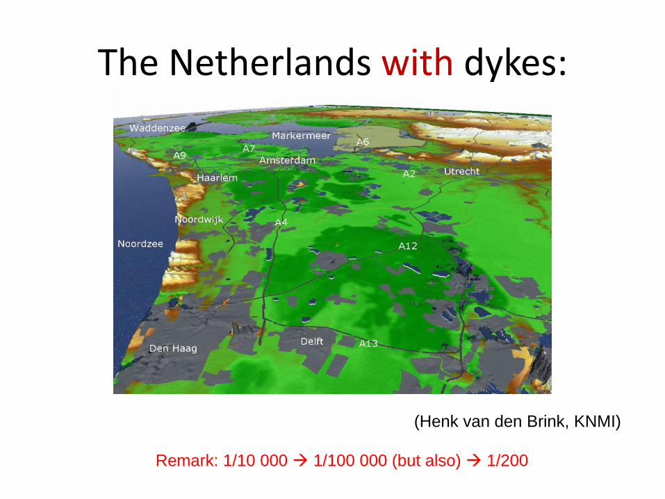
The Netherlands with dykes:
(Henk van den Brink, KNMI)
Remark: 1/10 000 1/100 000 (but also) 1/200
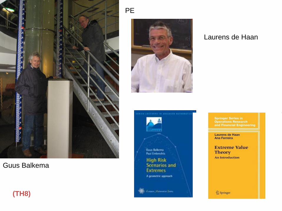
Guus Balkema
PE
Laurens de Haan
(TH8)
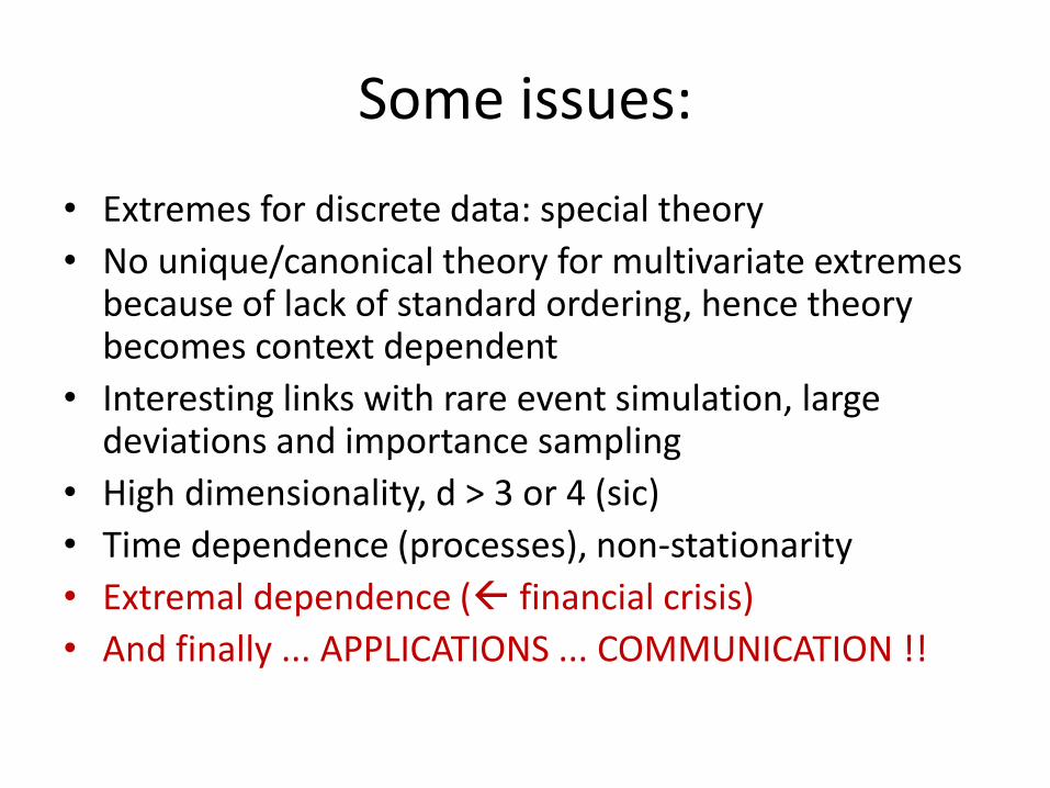
Some issues:
• Extremes for discrete data: special theory
• No unique/canonical theory for multivariate extremes because of lack of standard ordering, hence theory becomes context dependent
• Interesting links with rare event simulation, large deviations and importance sampling
• High dimensionality, d > 3 or 4 (sic)
• Time dependence (processes), non-stationarity
• Extremal dependence ( financial crisis)
• And finally ... APPLICATIONS ... COMMUNICATION !!

Thank you!