the multidisciplinary design problem as a dynamical …
TRANSCRIPT

THE MULTIDISCIPLINARY DESIGN PROBLEM AS ADYNAMICAL SYSTEM
A ThesisPresented to
The Academic Faculty
by
Bradley A. Steinfeldt
In Partial Fulfillmentof the Requirements for the Degree
Doctor of Philosophy in theSchool of Aerospace Engineering
Georgia Institute of TechnologyAugust 2013
Copyright c© 2013 by Bradley A. Steinfeldt
THE MULTIDISCIPLINARY DESIGN PROBLEM AS ADYNAMICAL SYSTEM
Approved by:
Dr. Robert D. Braun, AdvisorSchool of Aerospace EngineeringGeorgia Institute of Technology
Dr. Brian J. GermanSchool of Aerospace EngineeringGeorgia Institute of Technology
Mr. Gregg H. BartonMission Design GroupC. S. Draper Laboratory, Inc.
Dr. Panagiotis TsiotrasSchool of Aerospace EngineeringGeorgia Institute of Technology
Dr. Ian G. ClarkEntry, Descent, and Landing andAdvanced Techologies GroupJet Propulsion Laboratory
Date Approved: June 24, 2013

To my parents, Brian E. and M. Annette Steinfeldt.
To my maternal grandparents, William P. and Jean T. Alexander.
To my paternal grandparents, Wayne F. and Margaret M. Steinfeldt.
I’m on my feet, I’m on the floor, I’m good to go
So come on Davey, sing me something that I know
—Jimmy Eat World
iii

ACKNOWLEDGEMENTS
There are really no words that can adequately acknowledge the support of the nu-
merous people I have received during the course of my graduate career. However, I
will try to briefly acknowledge just a few of those who made this research possible.
To begin with, I have been honored to have had the opportunity to learn from my
advisor, Prof. Robert Braun. You have taught me more than you know and have
helped to shape me to be the engineer and person I am today. The patience, support,
fervor, perceptiveness, wisdom, savvy, scholarship, clarity, and ingenuity that you
have shown me throughout my graduate studies is truly remarkable. Thank you.
The guidance provided by my committee has been invaluable throughout the
development of this research. I owe each of you my heartfelt gratitude for your time
and dedication to making this work what it is today. Mr. Gregg Barton, your
support and mentoring throughout the years, while performing this research and
at Draper is appreciated more than words can express, thanks. Dr. Ian Clark,
thank you for your thoughts, advisement, and intellectual curiosity during your time
at Georgia Tech and while serving on my committee. Prof. Brian German, you
provided a plethora of knowledge, resources, and encouragement during this endeavor,
thank you. Prof. Panagiotis Tsiotras, I truly appreciate the direction and push
to stretch myself that you provided both in class and while developing this thesis.
Throughout the majority of my graduate career, I have been supported by the
Charles Stark Draper Laboratory, both on-campus and through summer work experi-
ences. They embody their original mission of “pioneer[ing] in science and technology,
contribut[ing] to the national interest, and promot[ing] the transfer of technology
through education.” I would like to acknowledge just a few of the people that have
iv

made my interactions with Draper special—Amer Fejzic, David Woffinden, Linda
Fuhrman, Mark Jackson, Matt Fritz, Phil Hattis, Scott Thompson, Seamus
Tuohy, and Steve Paschall.
I have been fortunate to be part of the Space System Design Lab (SSDL) dur-
ing my graduate career, without the support of many its members this work would
not have happened. These folks have not just been colleagues, they have provided a
fervent sounding board, support network, and social outlet for me while at Georgia
Tech. Mike Grant, with whom I took all but one class, took qualifying exams,
and performed countless hours of research—I do not know what to say, buddy, I
would not be who I am or know as much as I do without you. Thanks! Ashley
Korzun, Ben Stahl, Chris Cordell, Chris Tanner, Grant Rossman, Gregory
Lantoine, Ian Meginnis, Jarret Lafleur, Jenny Kelly, Jimmy Young, Milad
Mahzari, Nitin Arora, Patrick Chai, Richard Otero, Som Dutta, Zach Put-
nam, Zarrin Chua, and the rest of my labmates throughout the years in the SSDL,
thank each of you for being the definition of scholars and for your companionship.
In addition to my companions in the SSDL, many more friends supported me
through this journey. Andrzej Stewart, Antja Chambers, Ashley Tarpley,
Brad Maxwell, Jeff Story, Jerred Chute, Nina Patel, Shaun Tarpley, Suzanne
Oliason, and Yvonne Stephens are just a few of these friends. You are all phe-
nomenal for putting up with me, thanks!
Finally, this work would not have been possible without the unconditional love
and support of my family. Mom and Dad, you instilled a thirst for knowledge early
on and have done whatever it takes to enable me to satisfy that thirst. Thank you for
all of your sacrifices that have empowered me to follow my dreams. Grandma and
Granddaddy Alexander, thank you for the flawless guidance and the push to be
the best Brad I can be. Grandpa Steinfeldt thank you and Grandma Steinfeldt
for being amongst my strongest advocates and instilling a sense of passion in me.
v

TABLE OF CONTENTS
DEDICATION . . . . . . . . . . . . . . . . . . . . . . . . . . . . . . . . . . iii
ACKNOWLEDGEMENTS . . . . . . . . . . . . . . . . . . . . . . . . . . iv
LIST OF TABLES . . . . . . . . . . . . . . . . . . . . . . . . . . . . . . . xi
LIST OF FIGURES . . . . . . . . . . . . . . . . . . . . . . . . . . . . . . xii
NOMENCLATURE . . . . . . . . . . . . . . . . . . . . . . . . . . . . . . . xvi
SUMMARY . . . . . . . . . . . . . . . . . . . . . . . . . . . . . . . . . . . .xxviii
I BACKGROUND AND MOTIVATION . . . . . . . . . . . . . . . . 1
1.1 Multidisciplinary Design . . . . . . . . . . . . . . . . . . . . . . . . 1
1.1.1 Multidisciplinary Analysis vs. Design . . . . . . . . . . . . . 4
1.1.2 Multidisciplinary Design Representations . . . . . . . . . . . 5
1.1.3 Multidisciplinary Design Optimization . . . . . . . . . . . . . 7
1.2 Robust Multidisciplinary Design . . . . . . . . . . . . . . . . . . . . 11
1.2.1 Design Uncertainty . . . . . . . . . . . . . . . . . . . . . . . 11
1.2.2 Propagating Uncertainty . . . . . . . . . . . . . . . . . . . . 12
1.2.3 Robust Design . . . . . . . . . . . . . . . . . . . . . . . . . . 15
1.2.4 Robust Multidisciplinary Design . . . . . . . . . . . . . . . . 19
1.3 Dynamical Systems . . . . . . . . . . . . . . . . . . . . . . . . . . . 20
1.4 Previous Use of Dynamical System Concepts in Multidisciplinary Design 23
1.5 Study Overview and Objectives . . . . . . . . . . . . . . . . . . . . 26
1.6 Thesis Organization . . . . . . . . . . . . . . . . . . . . . . . . . . . 27
1.7 Academic Contributions . . . . . . . . . . . . . . . . . . . . . . . . . 29
II CASTING THE MULTIDISCIPLINARY DESIGN PROBLEM ASA DYNAMICAL SYSTEM . . . . . . . . . . . . . . . . . . . . . . . 32
2.1 Enabling Theoretical Foundations . . . . . . . . . . . . . . . . . . . 32
2.1.1 The Concept of a State . . . . . . . . . . . . . . . . . . . . . 32
2.1.2 Mathematical Definition of a Dynamical System . . . . . . . 33
vi
2.1.3 Discrete Dynamical Systems . . . . . . . . . . . . . . . . . . 34
2.1.4 Root-Finding Methods . . . . . . . . . . . . . . . . . . . . . 35
2.1.5 The Covariance Matrix . . . . . . . . . . . . . . . . . . . . . 40
2.1.6 Propagating Uncertainty . . . . . . . . . . . . . . . . . . . . 41
2.1.7 Matrix Norms . . . . . . . . . . . . . . . . . . . . . . . . . . 44
2.2 Multidisciplinary Design as a Dynamical System . . . . . . . . . . . 45
2.2.1 Identification of Feasible Designs . . . . . . . . . . . . . . . . 45
2.2.2 Design Optimization . . . . . . . . . . . . . . . . . . . . . . . 46
2.2.3 Identifying an Optimal Multidisciplinary Design . . . . . . . 46
2.2.4 Analog of Dynamical System Variables and MultidisciplinaryDesign Variables . . . . . . . . . . . . . . . . . . . . . . . . . 47
2.3 Summary . . . . . . . . . . . . . . . . . . . . . . . . . . . . . . . . . 48
III APPLYING DYNAMICAL SYSTEM THEORY TO MULTIDIS-CIPLINARY DESIGN . . . . . . . . . . . . . . . . . . . . . . . . . . 49
3.1 Design Convergence Using Stability Concepts . . . . . . . . . . . . . 49
3.1.1 Foundations of Stability Analysis . . . . . . . . . . . . . . . . 50
3.1.2 The Relationship of Stability to Design Convergence . . . . . 56
3.1.3 Region of Attraction . . . . . . . . . . . . . . . . . . . . . . . 56
3.1.4 Methods for Identifying the Stability of a System . . . . . . . 57
3.1.5 Estimating the Rate of Convergence Based on Lyapunov-likeTechniques . . . . . . . . . . . . . . . . . . . . . . . . . . . . 60
3.2 Design Constraints Using Optimal Control Theory . . . . . . . . . . 63
3.2.1 Continuous Dynamical Systems . . . . . . . . . . . . . . . . 63
3.2.2 Discrete Dynamical Systems . . . . . . . . . . . . . . . . . . 64
3.2.3 Solution Methods . . . . . . . . . . . . . . . . . . . . . . . . 66
3.2.4 Solution Search Coordination . . . . . . . . . . . . . . . . . . 67
3.3 Propagating Uncertainty Using Estimation Theory . . . . . . . . . . 68
3.3.1 The Discrete Kalman Filter . . . . . . . . . . . . . . . . . . . 69
3.3.2 Formulating the Multidisciplinary Design Problem in a FormCompatible with the Kalman Filter . . . . . . . . . . . . . . 69
vii
3.3.3 Using the Covariance Matrix to Guide Design Decomposition 70
3.4 Summary . . . . . . . . . . . . . . . . . . . . . . . . . . . . . . . . . 71
IV DEVELOPMENT OF A FRAMEWORK FOR THE RAPID RO-BUST DESIGN OF MULTIDISCIPLINARY SYSTEMS . . . . . 72
4.1 A Rapid Design Robustness Analysis Framework . . . . . . . . . . . 72
4.2 A Rapid Robust Design Methodology . . . . . . . . . . . . . . . . . 75
4.2.1 Formulation with Fixed-Point Iteration . . . . . . . . . . . . 75
4.2.2 Formulation with Newton-Raphson Iteration . . . . . . . . . 83
4.3 Summary . . . . . . . . . . . . . . . . . . . . . . . . . . . . . . . . . 85
V DEMONSTRATION OF DYNAMICAL SYSTEM THEORY AP-PLIED TO THE MULTIDISCIPLINARY DESIGN PROBLEM 87
5.1 Accuracy of the Mean and Variance Estimate . . . . . . . . . . . . . 87
5.1.1 Analytical Solution . . . . . . . . . . . . . . . . . . . . . . . 88
5.1.2 Rapid Robustness Assessment Methodology . . . . . . . . . . 89
5.1.3 Analysis Results . . . . . . . . . . . . . . . . . . . . . . . . . 93
5.2 Analysis of a Linear, Two Contributing Analysis Design . . . . . . . 98
5.3 Region and Rate of Convergence for a Nonlinear, Two ContributingAnalysis System . . . . . . . . . . . . . . . . . . . . . . . . . . . . . 101
5.4 Rapid Robust Design of a Linear, Three Contributing Analysis System102
5.4.1 Applying the Rapid Robust Design Methodology . . . . . . . 103
5.4.2 Design Results . . . . . . . . . . . . . . . . . . . . . . . . . . 107
5.5 Rapid Robust Design of a Two Bar Truss . . . . . . . . . . . . . . . 111
5.5.1 Applying the Rapid Robust Design Methodology . . . . . . . 113
5.5.2 Design Results . . . . . . . . . . . . . . . . . . . . . . . . . . 120
5.6 Rapid Robust Design of a Deployable for Strategic Vehicles . . . . . 121
5.6.1 Performance Impact of a Deployable System . . . . . . . . . 122
5.6.2 Baseline Strategic System Characteristics . . . . . . . . . . . 125
5.6.3 Modeling . . . . . . . . . . . . . . . . . . . . . . . . . . . . . 126
5.6.4 Problem Setup . . . . . . . . . . . . . . . . . . . . . . . . . . 130
viii

5.6.5 Applying the Rapid Robust Design Methodology . . . . . . . 133
5.6.6 Design Results . . . . . . . . . . . . . . . . . . . . . . . . . . 137
5.6.7 Conclusions . . . . . . . . . . . . . . . . . . . . . . . . . . . 148
5.7 Summary . . . . . . . . . . . . . . . . . . . . . . . . . . . . . . . . . 148
VI COMPUTATIONAL PERFORMANCE OF THE RAPID ROBUSTDESIGN METHODOLOGY . . . . . . . . . . . . . . . . . . . . . . . 150
6.1 Computational Effect of Increasing the Design Complexity on theRapid Robust Design Methodology . . . . . . . . . . . . . . . . . . . 150
6.1.1 Test Problem Definition . . . . . . . . . . . . . . . . . . . . . 151
6.1.2 Individual Sensitivities . . . . . . . . . . . . . . . . . . . . . 153
6.1.3 Overall Complexity Metrics . . . . . . . . . . . . . . . . . . . 156
6.1.4 Computational Speed of the Rapid Robust Design Methodology160
6.2 The Accuracy of a Linear Technique . . . . . . . . . . . . . . . . . . 160
6.3 Conservatism of the Matrix Two-Norm . . . . . . . . . . . . . . . . 166
6.4 Summary . . . . . . . . . . . . . . . . . . . . . . . . . . . . . . . . . 168
VII SUMMARY AND FUTURE WORK . . . . . . . . . . . . . . . . . 170
7.1 Summary of Academic Contributions . . . . . . . . . . . . . . . . . 170
7.1.1 Formulation of the General Multidisciplinary Design Problemas a Dynamical System In Order to Leverage Established Tech-niques from Dynamical System Theory . . . . . . . . . . . . 170
7.1.2 Application of the Dynamical System Domain to the Multi-disciplinary Design Problem . . . . . . . . . . . . . . . . . . 171
7.1.3 Development of a Linear Technique for the Rapid Robust De-sign of a Multidisciplinary System . . . . . . . . . . . . . . . 173
7.1.4 Application of the Multidisciplinary Design Robustness Method-ology to a Design Example of Relevance to the Entry, Descent,and Landing Community . . . . . . . . . . . . . . . . . . . . 174
7.1.5 Traceability of Each Contribution . . . . . . . . . . . . . . . 174
7.2 Advantages of Viewing the Multidisciplinary Design Problem as aDynamical System . . . . . . . . . . . . . . . . . . . . . . . . . . . . 175
7.3 Limitations of the Rapid Robust Design Methodology . . . . . . . . 176
7.4 Suggestions for Future Work . . . . . . . . . . . . . . . . . . . . . . 177
ix
7.4.1 Additional Dynamical Systems Techniques . . . . . . . . . . 178
7.4.2 Extending the Use of the Rapid Robust Design Methodology 180
APPENDIX A — SELECT MATHEMATICAL CONCEPTS . . . 182
APPENDIX B — PUBLICATIONS . . . . . . . . . . . . . . . . . . . 204
REFERENCES . . . . . . . . . . . . . . . . . . . . . . . . . . . . . . . . . . 208
VITA . . . . . . . . . . . . . . . . . . . . . . . . . . . . . . . . . . . . . . . . 225
x
LIST OF TABLES
1 Types of uncertainty in the conceptual design process. . . . . . . . . 11
2 Some previous uses of dynamical system concepts in design. . . . . . 25
3 Analog between dynamical system variables and design variables. . . 48
4 Discrete dynamical system stability criterion. . . . . . . . . . . . . . . 56
5 Comparison of solution techniques. . . . . . . . . . . . . . . . . . . . 67
6 Parameter ranges to assess the validity of the rapid robust designmethodology. . . . . . . . . . . . . . . . . . . . . . . . . . . . . . . . 93
7 Comparison of the performance of the rapid robustness assessmentmethod with other multidisciplinary uncertainty assessment techniques. 100
8 Parameters for the robust design of a three contributing analysis system.107
9 Design results for the linear, three contributing analysis system. . . . 111
10 Parameters for the two-bar truss problem. . . . . . . . . . . . . . . . 113
11 Baseline strategic vehicle aerodynamics . . . . . . . . . . . . . . . . . 125
12 Parameter values for the design. . . . . . . . . . . . . . . . . . . . . . 131
13 Computational comparison between MOPSO and the Rapid RobustDesign Methodology. . . . . . . . . . . . . . . . . . . . . . . . . . . . 141
14 Computational comparison between MOPSO and the Rapid RobustDesign Methodology. . . . . . . . . . . . . . . . . . . . . . . . . . . . 147
15 Parameters used to examine the individual effect of complexity param-eters on the design. . . . . . . . . . . . . . . . . . . . . . . . . . . . . 154
16 Design cases used to evaluate the overall complexity metrics. . . . . . 159
17 Traceability of academic contributions. . . . . . . . . . . . . . . . . . 174
A.1 Multivariate mass and density function properties. . . . . . . . . . . . 185
xi
LIST OF FIGURES
1 Sample Design Structure Matrices for the design of (a) a launch vehicleand (b) an automobile engine. . . . . . . . . . . . . . . . . . . . . . . 7
2 Sample Design Structure Matrix for SSA. . . . . . . . . . . . . . . . . 9
3 Normal distribution. . . . . . . . . . . . . . . . . . . . . . . . . . . . 12
4 Visualization of the most probable point method with the most prob-able point locus. . . . . . . . . . . . . . . . . . . . . . . . . . . . . . . 14
5 Robust design optimization compared to traditional design optimization. 16
6 An ideal pendulum. . . . . . . . . . . . . . . . . . . . . . . . . . . . . 20
7 Newton’s method for numerically finding the root of a nonlinear equation. 22
8 Block diagram of a linear, discrete dynamical system. . . . . . . . . . 35
9 Visual represent ion of the fixed-point iteration root-finding method. . 37
10 Newton’s method for numerically finding the root of a nonlinear equation. 38
11 Visual representation of the matrix two-norm. . . . . . . . . . . . . . 45
12 Multidisciplinary design through root-finding. . . . . . . . . . . . . . 47
13 Visualization of the concept of stability. . . . . . . . . . . . . . . . . . 51
14 Visualization of state trajectories in (a) R2 × R and (b) R2 showingstability for a continuous dynamical system. . . . . . . . . . . . . . . 52
15 Feasible design space accounting for (a) design variable constraints onlyand (b) design variable and contributing analysis constraints. . . . . . 68
16 The decomposition of an entry system into a Design Structure Matrix. 76
17 Two-contributing analysis multidisciplinary design. . . . . . . . . . . 88
18 Maximum error for a two contributing analysis multidisciplinary designwith µup
= (0 0)T . . . . . . . . . . . . . . . . . . . . . . . . . . . . . 95
19 Maximum error for a two contributing analysis multidisciplinary designwith µup
= (100 0)T . . . . . . . . . . . . . . . . . . . . . . . . . . . . 96
20 Maximum error for a two contributing analysis multidisciplinary designwith µup
= (100 100)T . . . . . . . . . . . . . . . . . . . . . . . . . . . 97
21 Mean and variance error between the rapid linear robustness analysistechnique and Monte Carlo analysis. . . . . . . . . . . . . . . . . . . 99
xii
22 Mean and variance error between the rapid linear robustness analysistechnique and the unscented transform. . . . . . . . . . . . . . . . . . 99
23 Mean and variance error between the rapid linear robustness analysistechnique and fast probability integration. . . . . . . . . . . . . . . . 100
24 Cantilever beam with a tip load. . . . . . . . . . . . . . . . . . . . . . 101
25 Nonlinear two contributing analysis design. . . . . . . . . . . . . . . . 101
26 Three contributing analysis multidisciplinary design. . . . . . . . . . 102
27 Divergent behavior demonstrated by the fixed-point iteration system(ud = 1). . . . . . . . . . . . . . . . . . . . . . . . . . . . . . . . . . . 108
28 Convergent behavior demonstrated by the fixed-point iteration system(ud = 1). . . . . . . . . . . . . . . . . . . . . . . . . . . . . . . . . . . 109
29 Optimal robust designs found using an exact propagation of uncer-tainty (blue) and approximate bounding method (green). . . . . . . . 110
30 Two bar truss with a load at the mutual joint. . . . . . . . . . . . . . 112
31 Two bar truss design structure matrix. . . . . . . . . . . . . . . . . . 113
32 History of the modulus of the maximum eigenvalue of the two bar trusssystem with iteration. . . . . . . . . . . . . . . . . . . . . . . . . . . . 118
33 Deterministic and robust design of a two bar truss with a load at themutual joint. . . . . . . . . . . . . . . . . . . . . . . . . . . . . . . . 120
34 Variation of 2||Σy∗||2 with the mean objective function for the designof a two bar truss with a load at the mutual joint. . . . . . . . . . . . 121
35 Variation of (a) miss distance and (b) range showing sensitivity tolift-to-drag ratio and insensitivity to ballistic coefficient. . . . . . . . . 123
36 Geometry of the deployable device. . . . . . . . . . . . . . . . . . . . 124
37 Increase in the maximum lift-to-drag ratio of the entry system for asingle-delta deployable as a function of deployable size. . . . . . . . . 125
38 Baseline strategic vehicle characteristics. . . . . . . . . . . . . . . . . 126
39 Design structure matrix for the design of a deployable for a strategicsystem. . . . . . . . . . . . . . . . . . . . . . . . . . . . . . . . . . . . 126
40 Design solutions for range comparing the rapid robust design method-ology and a multiobjective particle swarm optimizer for a (a) bank-to-steer guidance algorithm and the (b) acceleration control guidancealgorithm. . . . . . . . . . . . . . . . . . . . . . . . . . . . . . . . . . 138
xiii
41 Design solutions for accuracy comparing the rapid robust design method-ology and a multiobjective particle swarm optimizer for a (a) bank-to-steer guidance algorithm and the (b) acceleration control guidancealgorithm. . . . . . . . . . . . . . . . . . . . . . . . . . . . . . . . . . 139
42 The (a) impact on L/D of constraining the CG position to be withinthe vehicle and (b) the normalized (relative to the vehicle’s diameter)distance outside the vehicle the CG needs to be to achieve (L/D)max. 142
43 Body flap deflection angle required to trim the vehicle at the theoreticalmaximum L/D. . . . . . . . . . . . . . . . . . . . . . . . . . . . . . . 143
44 Comparison of investigated deployable concepts showing the maximumachievable L/D accounting for trim considerations. . . . . . . . . . . 143
45 Design solutions for range comparing the rapid robust design method-ology and a multiobjective particle swarm optimizer for a (a) bank-to-steer guidance algorithm and the (b) acceleration control guidancealgorithm for the double-delta configuration. . . . . . . . . . . . . . . 145
46 Design solutions for accuracy comparing the rapid robust design method-ology and a multiobjective particle swarm optimizer for a (a) bank-to-steer guidance algorithm and the (b) acceleration control guidancealgorithm for the double-delta configuration. . . . . . . . . . . . . . . 146
47 General design structure matrix for analyzing the effect of design com-plexity. . . . . . . . . . . . . . . . . . . . . . . . . . . . . . . . . . . . 152
48 Increase in computational cost with (a) number of design variables, (b)number of contributing analyses, (c) nonlinearity of the CAs, and (d)nonlinearity of the response. . . . . . . . . . . . . . . . . . . . . . . . 154
49 Increase in computational cost with complexities using the (a) alge-braic complexity metric, (b) Jacobian complexity metric, (c) force-based clustering metric, and (d) input-output metric. . . . . . . . . . 159
50 Three contributing analysis design structure matrix for nonlinearityanalysis. . . . . . . . . . . . . . . . . . . . . . . . . . . . . . . . . . . 161
51 Ten contributing analysis design structure matrix for nonlinearity anal-ysis . . . . . . . . . . . . . . . . . . . . . . . . . . . . . . . . . . . . . 162
52 Variation in the computed accuracy of the rapid robust design method-ology with the degree of nonlinearity. Three different nonlinear func-tions are shown, (a) sin(y), (b) ln(y), and (c) (−1)y. . . . . . . . . . . 164
53 Nonlinear perturbation analysis using the function g2(y) = ln(y) withthe errors associated with the deployable design example superimposed. 165
54 Two-dimensional geometry associated with the matrix two-norm. . . 167
xiv

55 Maximum percent error due to the matrix two-norm approximation asa function of the dimensionality of the problem. . . . . . . . . . . . . 168
xv
NOMENCLATURE
Acronyms
CA Contributing Analysis
CBAero Configuration Based Aerodynamics tool
CG Center of Gravity
CO Collaborative Optimization
CSSUA Concurrent Subsystem Uncertainty Analysis
DeMAID Design Manager’s Aid for Intelligent Decomposition
DOE Design of Experiments
DSM Design Structure Matrix
EDL Entry, Descent, and Landing
FPI Fast Probability Integration
FPKE Fokker-Plank-Kolmogorov Equation
GN&C Guidance, Navigation, and Control
LMI Linear Matrix Inequality
MDA/O Multidisciplinary Design Analysis/Optimization
MDO Multidisciplinary Design Optimization
MOPSO Multi-objective Particle Swarm Optimizer
MSD Mean Squared Deviation
xvi
NASA National Aeronautics and Space Administration
NLP Nonlinear Programming
OBD Optimizer Based Decomposition
PERT Program Evaluation and Review Technique
RSE Response Surface Equation
RSM Response Surface Methodology
SADT Structured Analysis and Design Technique
SNOPT Sparse Nonlinear Optimization
SoS System of Systems
SSA System Sensitivity Analysis
SUA System Uncertainty Analysis
Roman Variables
q Heat rate
0q q × 1 vector of zeros
1q q × 1 vector of ones
Aj Matrix describing the state contribution of the jth contributing anal-
ysis, Aj ∈ Rlj×m
Ak Matrix describing the state components to the dynamical system at
iterate k
Bj Matrix describing the deterministic input contribution of the jth con-
tributing analysis, Bj ∈ Rlj×d
xvii
b(i) Vector that lies in the dual cone D(P(i))
Bk Matrix describing the input (control) components to the dynamical
system at iterate k
Cj Matrix describing the probabilistic input contribution of the jth con-
tributing analysis, Cj ∈ Rlj×p
Ck Matrix describing the state components to the output of the dynam-
ical system at iterate k
dj Bias associated with the jth contributing analysis, dj ∈ Rlj
Dk Matrix describing the input (control) components to the output of
the dynamical system at iterate k
f(·) Concatenation of the contributing analyses input-output relation-
ships
f(·) General state dynamical system relationship
Fi(·) Symmetric polynomial matrix used in the sum-of-squares problem
g(·) General output dynamical system relationship
g(·) Inequality design constraints
H Observation model
h(·) Equality design constraints
In×n The n× n identity matrix
K Kalman gain
M Matrix describing the linear combination of the pertinent contribut-
ing analyses outputs to the design’s response, M ∈ R1×q
xviii

p Design parameters
Q Covariance of the random noise associated with the model
Q Positive semi-definite matrix used in the sum-of-squares problem
Q Unitary matrix in Schur decomposition
R Covariance of the random noise associated with the observation of
the system
r Position vector
r(·) Design response
S Residual covariance
S Sample covariance matrix
s Vector of state constraints
ud Deterministic system-level inputs into the design, ud ∈ Rd
up Probabilistic system-level inputs into the design, up ∈ Rp
U Upper triangular matrix
u Control variable in the optimal control problem
u Design variables
V Matrix whose columns are the (generalized) eigenvectors
v Random noise associated with the observation of the system, v ∼
N (0,R)
w Random noise associated with the model, w ∼ N (0,Q)
xix
w(y) Equality constraints that are a function of the state
Wk Complex-valued matrix
yj Contributing analysis output, yj ∈ Rlj
y Concatenation of all contributing analyses output, the state variable,
y ∈ Rm
z State observation
z(·) Column vector in the sum-of-squares problem whose entries are mono-
mial in (·)
A Area
a Ellipsoid semi-major axis
b Ellipsoid semi-minor axis
CD Drag coefficient
ci Weighting variable in the sum-of-squares solution
CL Lift coefficient
d Dimensionality of the deterministic inputs, i.e., d = dim(ud)
dmiss Miss distance
E Young’s modulus
f Force magnitude
f(·) Arbitrary scalar mapping
fuy(u,p) Joint probability distribution function of u and p
xx
g Magnitude of the acceleration due to gravity
g(·) Scalar arbitrary function
H Atmospheric scale height
h Altitude
H(·) Hamiltonian
I Mass moment of inertia
k Iterate index
kk Dimensionality of the control equality constraints in the discrete op-
timal control problem
ks Sutton-Graves constant
kCDDrag coefficient multiplier
kCLLift coefficient multiplier
l Length
L(·) Lagrangian
L/D Lift-to-drag ratio
l/d Deployable length to vehicle diameter ratio
lj Dimensionality of the jth contributing analysis’s output, i.e., lj =
dim(yj)
m Dimensionality of the concatenated contributing analyses’s outputs,
m =n∑i=1
lj
xxi

m Mass
n Number of contributing analyses
p Deployable internal pressure
p Dimensionality of the probabilistic inputs, i.e., p = dim(up)
pk Dimensionality of the state equality constraints in the discrete opti-
mal control problem
Q Integrated heat load
q Dimensionality of the pertinent contributing analyses’ responses that
contribute to the design objective
q Order of the contributing analyses
qk Dimensionality of the control inequality constraints in the discrete
optimal control problem
r Order of the response
r Radius
rk Dimensionality of the state inequality constraints in the discrete op-
timal control problem
rn Stagnation radius
s Dimensionality of the input space, s = d+ p
T Tension
t Dimensionality of the response
v Velocity magnitude
xxii
V (·) Lyapunov function
vi(·) Monomial function in (·)
W Weight
w Constant factor for exponential stability
w Parameter weights
w(·) Mapping from Rn → R that is continuous at the equilibrium point
z Ellipsoid altitude
Greek Variables
α Scaling factor or weight on the mean value
β Ballistic coefficient, β =m
CDA
β Reduction factor for exponential systems
β Scaling factor or weight on the spread of the distribution
β Deterministic input contribution in the fixed-point iteration equa-
tion, β ∈ Rm×d
δ Bias in the fixed-point iteration equation, δ ∈ Rm
γ Probabilistic input contribution in the fixed-point iteration equation,
γ ∈ Rm×p
Λ State contribution in the fixed-point iteration equation, Λ ∈ Rm×m
λ Lagrange multiplier
µ Lagrange multiplier
xxiii

ν Lagrange multiplier
ω(y) Inequality constraints that are a function of the state
Φ(k, j) Discrete state transition matrix from iterate k to iterate j
Ψ Matrix transformation
Σ Covariance matrix
ζ Transformation variable
δ Deployable material thickness
ε Convergence tolerance
γ Flight path angle
κ(·) Function describing a mapping from Cn×n → R
µ Mean value (µ(·) = E(·))
µg Gravitational parameter
ν Poisson’s ratio
Ω Set of objective functions
φ Longitude
φ(·) Continuous function describing a mapping from Rn → R
φ(·) Terminal state cost
ψ Heading angle
ρ Density
ρXi,XjProduct-moment coefficient between Xi and Xj, ρXi,Xj
∈ [−1, 1]
xxiv
Σ Set of admissible states
σ Bank angle
σ Standard deviation (σ(·) =√σ2
(·) =√E((·)− E(·))2 =
√E((·)− µ(·))2
σ2 Variance (σ2(·) = E((·)− E(·))2 = E((·)− µ(·))
2)
σt Material tensile strength
σy Yield strength
θ Latitude
λi Set of eigenvalues
Script Variables
A Region of attraction
Cn[a, b] n times continuously differentiable function on the interval [a, b]
D Open neighborhood of the equilibrium point
J (·) Objective function
L(·) Optimal control path cost
N (µ,Σ) Normal random variable with mean µ and covariance Σ
N (µ, σ2) Normal random variable with mean µ and variance σ2
O Big-O complexity
P(i) Convex cone for the discrete optimal control problem
Q(i) Convex cone for the discrete optimal control problem
S Set of sigma points used in the unscented transform, S = σi
xxv
T Set of times
U Set of admissible inputs (controls)
U(xmin, xmax) Uniform random variable which varies between xmin and xmax
V Set of Lyapunov function candidates
Xs Domain of exponential stability
Y Set of output functions
X i Set of trial points used in the unscented transform
Y i Set of propagated trial points used in the unscented transform
Variable Superscripts and Subscripts
(·)e Equilibrium of (·)
(·)∗ Root value or optimum value of (·)
(·)0 Initial value of (·)
(·)f Final value of (·)
(·)k Iterate k of (·)
(·)T Target value of (·)
(·)accuracy Accuracy of (·)
(·)baseline Reference to the baseline of (·)
(·)j|k Estimate at j given observations up to and including k
(·)miss Miss distance of (·)
(·)nom Nominal value of (·)
xxvi
(·)vert Vertical component of (·)
(·) Mean value of (·)
(·) Estimate of the mean of (·)
(·) Nominal value of (·)
Functions and Operators
(·)H Conjugate transpose of (·)
(·)T Transpose of (·)
(·)−1 Inverse of (·)
=(·) Imaginary part of (·)
λmax(·) Function which returns the maximum eigenvalue of (·)
E(·) Mathematical expectation of (·)
<(·) Real part of (·)
P [(·)] Function which returns the probability of (·)
Spaces
C Set of complex numbers
R Set of real numbers
R+ Set of all positive real numbers (i.e., R+ = x : x ∈ [0,∞))
Z Set of all integers
Z+ Set of all positive integers (i.e., Z+ = 0, 1, 2, 3, . . .)
xxvii
SUMMARY
The design of complex systems requires of analyses from numerous disciplines.
When each of the disciplines use the same information, have a common set of as-
sumptions, and satisfy the constraints imposed on the design, the design is said to be
converged. The convergence process for complex, multidisciplinary designs may be
lengthy. Finding an optimal design can be computationally burdensome, particularly
for design space exploration when uncertainties are considered. Dynamical systems
theory has established techniques for their analysis. Exploiting an analog between
the multidisciplinary design problem and dynamical systems enables leveraging of
these resources in a new domain. Viewing the multidisciplinary design process as a
dynamical system broadens the computational tools available, increases the number
of analyses that can be performed, and potentially speeds the design-analysis cy-
cle. Casting this problem as a dynamical system is a departure from the developed
techniques applied in multidisciplinary design.
Finding a converged multidisciplinary design can be thought of as a multidimen-
sional root-finding problem. The numerical process to identify the roots of the design
is typically an iterative one, where subsequent iteration relies on information from
prior iterates. This iteration scheme can employ methods from dynamical systems
theory, which evolves a state by a fixed rule. In this work, it is shown that use of
root-finding techniques allows the multidisciplinary design problem to be recast as a
dynamical system enabling rapid solution using established theory.
In this investigation, theoretical foundations are developed for casting the mul-
tidisciplinary design problem as a discrete dynamical system, including handling of
xxviii
constraints within the design. Three particular techniques from the domain of dy-
namical system theory are developed and utilized to yield a linear rapid robust design
methodology.
1. Stability analysis: The existence of a converged design (for a given iteration
scheme) is shown to be determinable using dynamical system stability analysis,
where the conditions for asymptotic stability are shown to be identically equal
to those required for convergence.
2. Optimal control: Constraints on the design variables and outputs of the
contributing analyses are shown to be accommodated in a similar way that
state and control constraints are treated in optimal control theory. Adjoining
conditions to the objective function allows handling of both of these constraint
types at the same level of the optimization hierarchy.
3. Estimation theory: A design’s robustness characteristics (i.e., the mean and
variance) is shown to be analyzable using a Kalman filter (for linear designs),
where the mean state and covariance matrix are products of propagating the
filter until the design converges. This technique allows for the accounting of
uncertainties within the model itself as well as within the parameters of the
design.
Each of these dynamical systems techniques is demonstrated independently as
well as in an ensemble in the robust design of engineering systems. As an ensemble,
a rapid methodology for robust multidisciplinary design is formulated which finds a
conservative upper bound of the variance of the design to a scalar objective function.
Analytic test problems are solved to illustrate the benefits of this approach. The
developed methodology is then applied to the design of a deployable aerodynamic
surface for a strategic system in which an increase in range or an improvement in
landed accuracy is sought.
xxix
CHAPTER I
BACKGROUND AND MOTIVATION
1.1 Multidisciplinary Design
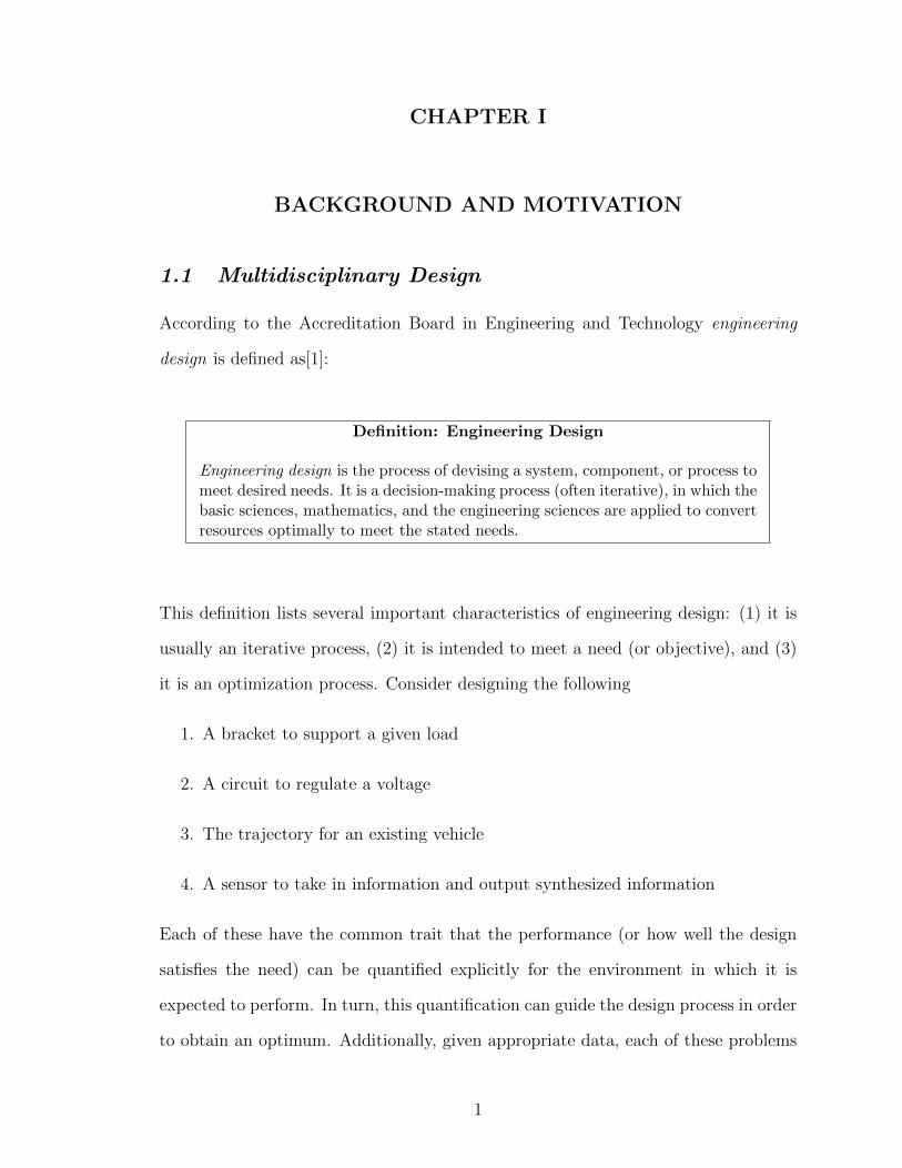
According to the Accreditation Board in Engineering and Technology engineering
design is defined as[1]:
Definition: Engineering Design
Engineering design is the process of devising a system, component, or process tomeet desired needs. It is a decision-making process (often iterative), in which thebasic sciences, mathematics, and the engineering sciences are applied to convertresources optimally to meet the stated needs.
This definition lists several important characteristics of engineering design: (1) it is
usually an iterative process, (2) it is intended to meet a need (or objective), and (3)
it is an optimization process. Consider designing the following
1. A bracket to support a given load
2. A circuit to regulate a voltage
3. The trajectory for an existing vehicle
4. A sensor to take in information and output synthesized information
Each of these have the common trait that the performance (or how well the design
satisfies the need) can be quantified explicitly for the environment in which it is
expected to perform. In turn, this quantification can guide the design process in order
to obtain an optimum. Additionally, given appropriate data, each of these problems
1
can be designed by a single discipline without the need for outside interaction. Often,
the system, component, or process being designed is comprised of many components
and disciplines that must have interaction with each other in order to obtain a design
that fulfills the stated need. Such is the case when designing
1. A wing for an aircraft
2. A bridge across a body of water
3. A robot that autonomously cleans the floors of a house
Ackoff defines a system as[2]
Definition: System
A system is a set of two or more interrelated elements of any kind that satisfiesthe following conditions:
1. The properties or behavior of each element of the set has an effect on theproperties or behavior of the set taken as a whole.
2. The properties and behavior of each element, and the way they affect thewhole, depend on the properties and behavior of at least one other elementin the set. Therefore, no part has an independent effect on the whole andeach is affected by at least one other part.
3. Every possible subgroup of elements in the set has the first two properties:each has a nonindependent effect on the whole. Therefore, the wholecannot be decomposed into independent subsets. A system cannot besubdivided into independent subsystems.
The definition of a system can be extended to include complex systems. For complex
systems, there are many contributing analyses (CAs) that contribute to the complete
design of the system. The CAs in the design represent an analysis, process, or subsys-
tem in the design of the complex system. In addition, there is generally some control
of the inputs into each of the CAs that govern the solution process. This leads to the
following extension of the engineering design definition for complex systems.
2
Definition: Complex System Design
Complex system design is an engineering design where the system, component,or process being designed to meet desired needs is made up of a hierarchy ofsystems, components, or processes.
When each of the CAs is thought of as a system in and of itself, the complex system
may also be referred to as a System of Systems (SoS). There are many definitions of
a SoS[3, 4, 5, 6, 7, 8, 9, 10]. Each has separate requirements, such as those in Ref.
[9] which require that for a complex system to be a SoS each of the CAs must be in-
dependent, have some form of communication, and work towards a common mission.
Whereas Ref. [3] requires that a SoS have operational and managerial independence,
geographic distribution, emergent behavior, and evolutionary development. The com-
mon thread for each of these definitions is that the complex system is composed of
several CAs that may each be thought of as systems themselves.
It may be the case in complex system design where the CAs span different domains
of expertise (e.g., structures, trajectory, and budget) and design decisions made in
one discipline significantly affect the performance in another discipline. In this case,
the complex system is referred to as a multidisciplinary design.
Definition: Multidisciplinary Design
Multidisciplinary design is the engineering design of a complex system in whichat least two of the contributing analyses are from domains of different disciplinesand the performance of one discipline is affected by design decisions in anotherdiscipline.
Inherently the design of most aerospace systems is multidisciplinary, which is why
it is the multidisciplinary design context that this research is built upon.
3
1.1.1 Multidisciplinary Analysis vs. Design
Multidisciplinary analysis problems and multidisciplinary design problems are funda-
mentally complementary—design is an extension of analysis. The difference between
the analysis problem and the design problem lies in the existence of requirements.
These requirements are constraints that the system, component, or process must
meet. In addition, the design problem has a sense of optimality associated with it.
One solution to the multidisciplinary design problem involves wrapping an optimizer
around a multidisciplinary analysis framework for the desired problem. Constraints
in the optimization procedure are then obtained by either directly or indirectly trans-
lating the requirements on the system. In the research that follows, it is in this
sense that the multidisciplinary design problem is approached, one where the design
requirements are handled as constraints. That is, in the research that follows multi-
disciplinary design means the process of finding a vector of design variables, u, for a
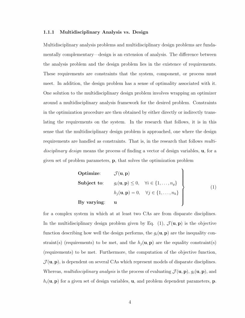
given set of problem parameters, p, that solves the optimization problem
Optimize: J (u,p)
Subject to: gi(u,p) ≤ 0, ∀i ∈ 1, . . . , ng
hj(u,p) = 0, ∀j ∈ 1, . . . , nh
By varying: u
(1)
for a complex system in which at at least two CAs are from disparate disciplines.
In the multidisciplinary design problem given by Eq. (1), J (u,p) is the objective
function describing how well the design performs, the gi(u,p) are the inequality con-
straint(s) (requirements) to be met, and the hj(u,p) are the equality constraint(s)
(requirements) to be met. Furthermore, the computation of the objective function,
J (u,p), is dependent on several CAs which represent models of disparate disciplines.
Whereas, multidisciplinary analysis is the process of evaluating J (u,p), gi(u,p), and
hi(u,p) for a given set of design variables, u, and problem dependent parameters, p.
4
1.1.2 Multidisciplinary Design Representations
The vast amount of information required to complete a design, particularly in multi-
disciplinary problems, can be managed by using a graphical representation of the
design. The decomposition of a design into appropriate CAs and identification
of information flow has been shown to provide perceptive insight into the design
process[11, 12, 13, 14]. The flow of information contributes significantly to the dif-
ficulty of the problem[11]. Consider the case when a CA relies on information of a
subsequent CA, this is known as a coupled design as the first CA must make as-
sumptions on the information provided by the second and the two must iterate until
the information used between the two CAs is consistent. This is a more difficult
problem than the non-iterative problem posed when the first CA did not rely on any
information from a subsequent CA.
Several traditional techniques exist for the graphical representation of multidisci-
plinary designs. Amongst these techniques are directed graphs, or digraphs, Program
Evaluation and Review Technique (PERT) diagrams, Structured Analysis and Design
Technique (SADT) diagrams, and Design Structure Matrices (DSMs) .
Directed graphs represent the design as a mapping of interconnected nodes. In
this representation, the nodes represent the CAs and the links represent the infor-
mation transfer from one CA to another CA and the direction of this transfer[15].
However, node locations are arbitrarily decided which can lend itself to a cluttered
and seemingly non-informative diagram for complex systems. PERT diagrams use
the fundamental concepts of the directed graphs; however PERT diagrams exhibit an
element of time. In this representation, nodes represent milestones of the design with
the distance between the nodes representing the time. Along each link between the
nodes are the CAs that need to be completed between milestones[16]. The benefit of
such a representation is the ability to rapidly identify the critical path of the project
and project completion. The downside to the traditional PERT diagram, is that they
5
lose information regarding the sequence of the CAs between milestones and in par-
ticular any iteration that may be required between CAs. SADT represents designs
as a system of interconnected boxes and arrows. This method splits out the directed
graphs into a box diagram representation. Each CA is its own box diagram and
then the CAs are integrated together at a high level. The benefit of SADT is that it
allows a structured way to show the information contained within a directed graph,
including information feedback. However, ultimately the SADT diagrams provide
only a glimpse into the design because the actual information flow from a high level
between multiple CAs is not immediately evident without looking within multiple
box diagrams. DSMs address the primary shortcomings of the previous techniques
by imposing a structure to the design representation. A DSM is a square matrix
which maps the information flow between CAs. In the static sense, a DSM is referred
to as an N2 diagram, because if the design is composed on N CAs, the matrix’s
dimension is N×N [17]. Within the DSM, the nodes along the diagonal of the matrix
are the representative CAs while the off-diagonal elements represent information flow.
In particular, for a matrix A, element aij, i 6= j is non-zero (represented by a dot)
if node i provides information to node j. Feedback is readily identified using this
technique if aij 6= 0, i > j.
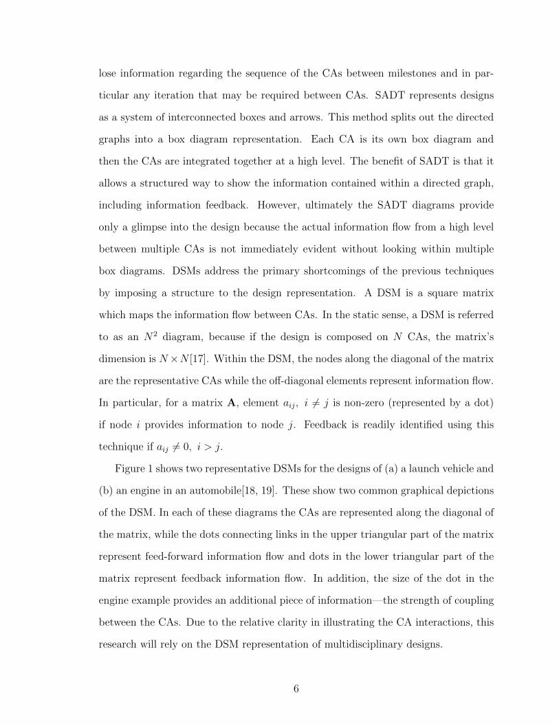
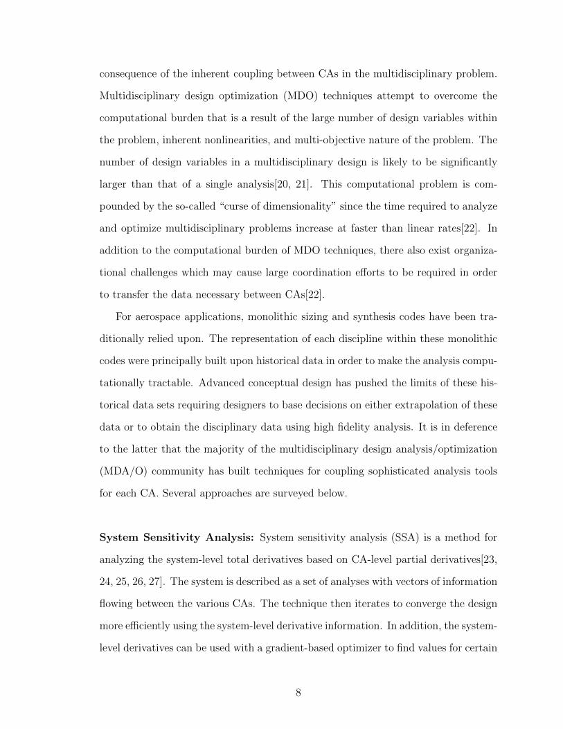
Figure 1 shows two representative DSMs for the designs of (a) a launch vehicle and
(b) an engine in an automobile[18, 19]. These show two common graphical depictions
of the DSM. In each of these diagrams the CAs are represented along the diagonal of
the matrix, while the dots connecting links in the upper triangular part of the matrix
represent feed-forward information flow and dots in the lower triangular part of the
matrix represent feedback information flow. In addition, the size of the dot in the
engine example provides an additional piece of information—the strength of coupling
between the CAs. Due to the relative clarity in illustrating the CA interactions, this
research will rely on the DSM representation of multidisciplinary designs.
6
(a)
(b)
Figure 1: Sample Design Structure Matrices for the design of (a) a launch vehicle and(b) an automobile engine.
1.1.3 Multidisciplinary Design Optimization
As discussed previously, engineering design implies that there is an optimal solu-
tion. The process of identifying this optimum requires implementing a methodology
that is more sophisticated than that required by single discipline systems. This is a
7
consequence of the inherent coupling between CAs in the multidisciplinary problem.
Multidisciplinary design optimization (MDO) techniques attempt to overcome the
computational burden that is a result of the large number of design variables within
the problem, inherent nonlinearities, and multi-objective nature of the problem. The
number of design variables in a multidisciplinary design is likely to be significantly
larger than that of a single analysis[20, 21]. This computational problem is com-
pounded by the so-called “curse of dimensionality” since the time required to analyze
and optimize multidisciplinary problems increase at faster than linear rates[22]. In
addition to the computational burden of MDO techniques, there also exist organiza-
tional challenges which may cause large coordination efforts to be required in order
to transfer the data necessary between CAs[22].
For aerospace applications, monolithic sizing and synthesis codes have been tra-
ditionally relied upon. The representation of each discipline within these monolithic
codes were principally built upon historical data in order to make the analysis compu-
tationally tractable. Advanced conceptual design has pushed the limits of these his-
torical data sets requiring designers to base decisions on either extrapolation of these
data or to obtain the disciplinary data using high fidelity analysis. It is in deference
to the latter that the majority of the multidisciplinary design analysis/optimization
(MDA/O) community has built techniques for coupling sophisticated analysis tools
for each CA. Several approaches are surveyed below.
System Sensitivity Analysis: System sensitivity analysis (SSA) is a method for
analyzing the system-level total derivatives based on CA-level partial derivatives[23,
24, 25, 26, 27]. The system is described as a set of analyses with vectors of information
flowing between the various CAs. The technique then iterates to converge the design
more efficiently using the system-level derivative information. In addition, the system-
level derivatives can be used with a gradient-based optimizer to find values for certain
8
system-level design variables that are able to be mathematically removed from the
CA level optimizers.
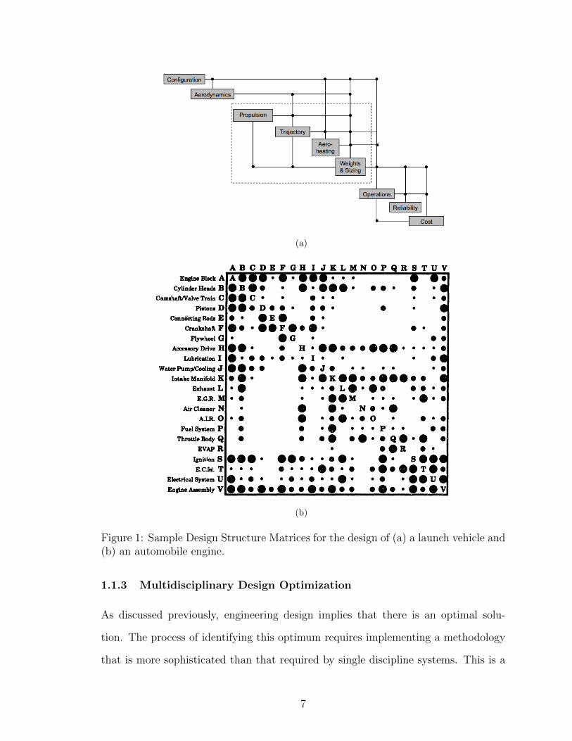
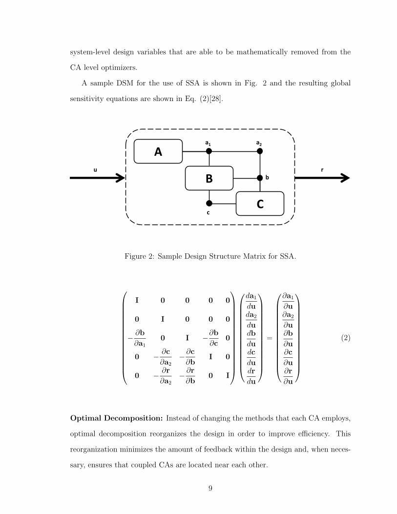
A sample DSM for the use of SSA is shown in Fig. 2 and the resulting global
sensitivity equations are shown in Eq. (2)[28].
A
B
C
a1 a2
b
c
u r
Figure 2: Sample Design Structure Matrix for SSA.
I 0 0 0 0
0 I 0 0 0
− ∂b
∂a1
0 I −∂b
∂c0
0 − ∂c
∂a2
− ∂c
∂bI 0
0 − ∂r
∂a2
− ∂r
∂b0 I
da1
duda2
dudb
dudc
dudr
du
=
∂a1
∂u∂a2
∂u∂b
∂u∂c
∂u∂r
∂u
(2)
Optimal Decomposition: Instead of changing the methods that each CA employs,
optimal decomposition reorganizes the design in order to improve efficiency. This
reorganization minimizes the amount of feedback within the design and, when neces-
sary, ensures that coupled CAs are located near each other.
9
One MDO software implementing optimal decomposition principles is the Design
Manager’s Aid for Intelligent Decomposition (DeMAID) developed at NASA’s Lang-
ley Research Center[29]. Given a DSM, relative coupling between CAs, and relative
computational expenses, DeMAID will find the optimal order of execution for the
multidisciplinary design. This is useful for the case when the DSM organization is
not intuitive. More recent methods for the optimal decomposition of a design rely
on mutual information to measure the data dependence between CAs or forced-based
clustering to discover the sub-graph structure within the design[30].
Optimizer-Based Decomposition: Optimizer-based decomposition (OBD) is a
single-level optimization method that eliminates feedforward and feedback loops.
The elimination of these loops is done through the use of compatibility constraints
which ensure a converged design uses consistent variable values for the coupling
variables[31, 32]. Additionally, the potential conflict between the system-level de-
sign objectives and CA-level design objectives are eliminated in OBD by allowing all
of the design variables to be chosen by the system-level optimizer.
Collaborative Optimization: Collaborative Optimization (CO) is a bi-level de-
composition technique where the system level optimizer coordinates the optimization
at the lower CA level in order to achieve an overall system objective[33, 34, 31, 35,
36, 37, 38]. The coupling between CAs is handled through compatibility constraints
as with OBD; however, these constraints are implemented by assessing the differ-
ence in the target value set at the system-level and the actual values used by the
CAs. The unique implementation of the compatibility constraints allows distributed
optimization of the problem and is therefore more aptly scalable.
10

1.2 Robust Multidisciplinary Design
1.2.1 Design Uncertainty
Uncertainty is not knowing with certainty a value or an action. More formally, un-
certainty is defined as[39]
Definition: Uncertainty
Uncertainty is the quality or state of being indefinite or indeterminate.
The ramifications of uncertainty on design could potentially mean that a design that
meets the design requirements and objectives in a deterministic environment may not
do so when the design is assessed probabilistically. Uncertainty can be classified in
several categories as shown in Table 1.
Table 1: Types of uncertainty in the conceptual design process.
UncertaintyDescription Example Reference
SourceInaccuracies in Using an exponential [40], [41], [42],
Physical the physical atmosphere to [43], [44], [45],Modeling modeling of represent the [46], [47], [48],
the system actual atmosphere [49], [50], [51]Unknowns in Degraded performance
Unknown the operating or failure of aOperating environment satellite in a [52], [53], [54],Conditions of the system communications [55], [56], [28]
constellation
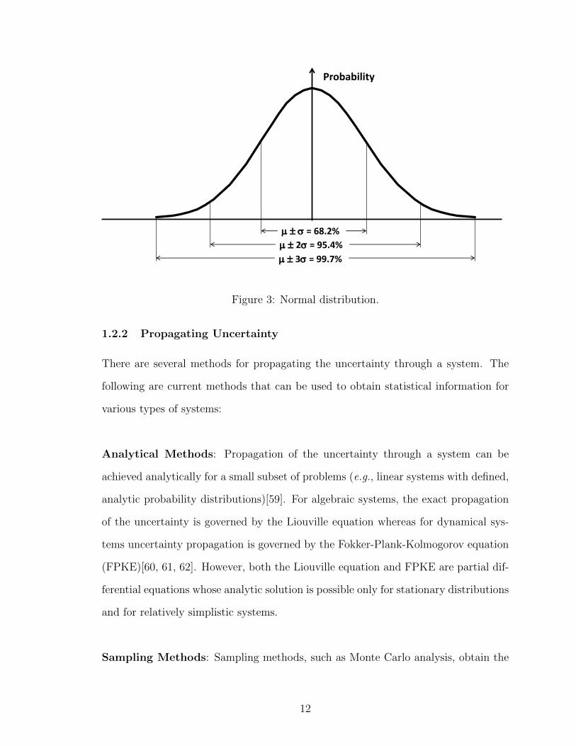
Within the design community, an accepted measure of design uncertainty is the
spread of the distribution. This can be characterized by the variance, σ2, or standard
deviation, σ, about the mean[57, 58]. Figure 3 shows a normal distribution and it
can be seen that the smaller the standard deviation (or variance), the tighter the
distribution, while a larger standard deviation (or variance) implies that the spread
of the distribution is large.
11
Probability
= 68.2%
2 = 95.4%
3 = 99.7%
Figure 3: Normal distribution.
1.2.2 Propagating Uncertainty
There are several methods for propagating the uncertainty through a system. The
following are current methods that can be used to obtain statistical information for
various types of systems:
Analytical Methods: Propagation of the uncertainty through a system can be
achieved analytically for a small subset of problems (e.g., linear systems with defined,
analytic probability distributions)[59]. For algebraic systems, the exact propagation
of the uncertainty is governed by the Liouville equation whereas for dynamical sys-
tems uncertainty propagation is governed by the Fokker-Plank-Kolmogorov equation
(FPKE)[60, 61, 62]. However, both the Liouville equation and FPKE are partial dif-
ferential equations whose analytic solution is possible only for stationary distributions
and for relatively simplistic systems.
Sampling Methods: Sampling methods, such as Monte Carlo analysis, obtain the
12

distribution of a given objective function by running successive deterministic sim-
ulations with values chosen from random distributions for the stochastic variables
associated with the problem[63]. The stochastic variables continue to be sampled
and evaluated in the deterministic simulation until a statistically stationary distri-
bution is obtained. The clear advantage of sampling methods are that for a large
enough sample size they give the probability distribution being sought and they pro-
vide statistical insight into the results. However, the computational runtime can be
prohibitive and only in the limit does the resultant probability distribution represent
true probability distribution. One way to bypass the computational runtime asso-
ciated with direct sampling is to use metamodeling techniques to create a curve fit
of the system’s response. This is called the response surface methodology (RSM)
[64, 65, 66, 67, 68]. Commonly, a quadratic equation is used and in this case, the
surrogate model is referred to as a second-order response surface equation (RSE) .
Most Probable Point Methods: Most probable point methods obtain an estimate
for the cumulative distribution function for probabilistic system design[69, 70, 71, 72,
73, 74, 75, 76, 77, 78, 79, 80, 81]. In particular, these methods take a known input
distribution and evaluate it against a constraint function that is a requirement of
the design. While there are a wide variety of techniques that can be classified as a
most probable point method, these methods generally transform the input distribu-
tion into the standard normal space where each of the random variables are assumed
to be independent. Using an approximation of the constraint, the first design point is
found by minimizing the distance to the mean of the probability density function in
standard normal space while satisfying the approximate constraint. The cumulative
distribution function is found by allowing the constraint value to vary (i.e., instead
of exactly satisfying the constraint function, it satisfies the constraint function plus
13
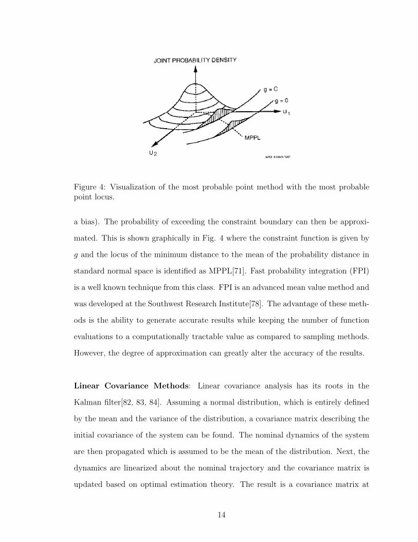
Figure 4: Visualization of the most probable point method with the most probablepoint locus.
a bias). The probability of exceeding the constraint boundary can then be approxi-
mated. This is shown graphically in Fig. 4 where the constraint function is given by
g and the locus of the minimum distance to the mean of the probability distance in
standard normal space is identified as MPPL[71]. Fast probability integration (FPI)
is a well known technique from this class. FPI is an advanced mean value method and
was developed at the Southwest Research Institute[78]. The advantage of these meth-
ods is the ability to generate accurate results while keeping the number of function
evaluations to a computationally tractable value as compared to sampling methods.
However, the degree of approximation can greatly alter the accuracy of the results.
Linear Covariance Methods: Linear covariance analysis has its roots in the
Kalman filter[82, 83, 84]. Assuming a normal distribution, which is entirely defined
by the mean and the variance of the distribution, a covariance matrix describing the
initial covariance of the system can be found. The nominal dynamics of the system
are then propagated which is assumed to be the mean of the distribution. Next, the
dynamics are linearized about the nominal trajectory and the covariance matrix is
updated based on optimal estimation theory. The result is a covariance matrix at
14
each point along the nominal dynamics which can be used to ascertain the joint prob-
ability density of the distribution. However, inherently the method does not allow
for the analysis of the algebraic systems since there is not a defined dynamical system.
Other Methods: There are several other techniques for propagating the uncertainty
through a system. For algebraic systems, these include techniques based on bound-
ing methods, differential analysis, Fourier analysis, polynomial chaos, and reliability
analysis[59, 85, 80, 86, 85, 79, 87, 88, 89]. For dynamic systems, these include the use
of numerical approximations to the FPKE equation, stochastic averaging, lineariza-
tion, Gaussian closure, and Gaussian mixture techniques[90, 91, 92, 93, 94, 95, 96, 97,
98]. All of these techniques rely on approximation techniques or are only applicable
in situations where the functional form of the system and distribution meet certain
requirements (e.g., the system is described by a polynomial).
1.2.3 Robust Design
In design the goal is traditionally to find the best solution to a given objective[99, 100,
101, 102, 103]. However, this optimum could lead to large variations in the objective
function around the optimum when the model or operating conditions are uncertain,
as is the case in the majority of engineering problems[33, 104]. This motivates the
need for robust design where the design is to perform as expected despite these un-
certainties.
Definition: Robust Design
Robust design is the process of devising a system, component, or process tomeet desired needs and meet a quality standard even in the presence of physicalmodeling uncertainties and unknown operating conditions.
A graphical depiction of robust design is shown in Fig. 5.
15
Performance
Environment
Robust Design
Optimal Design
Nominal
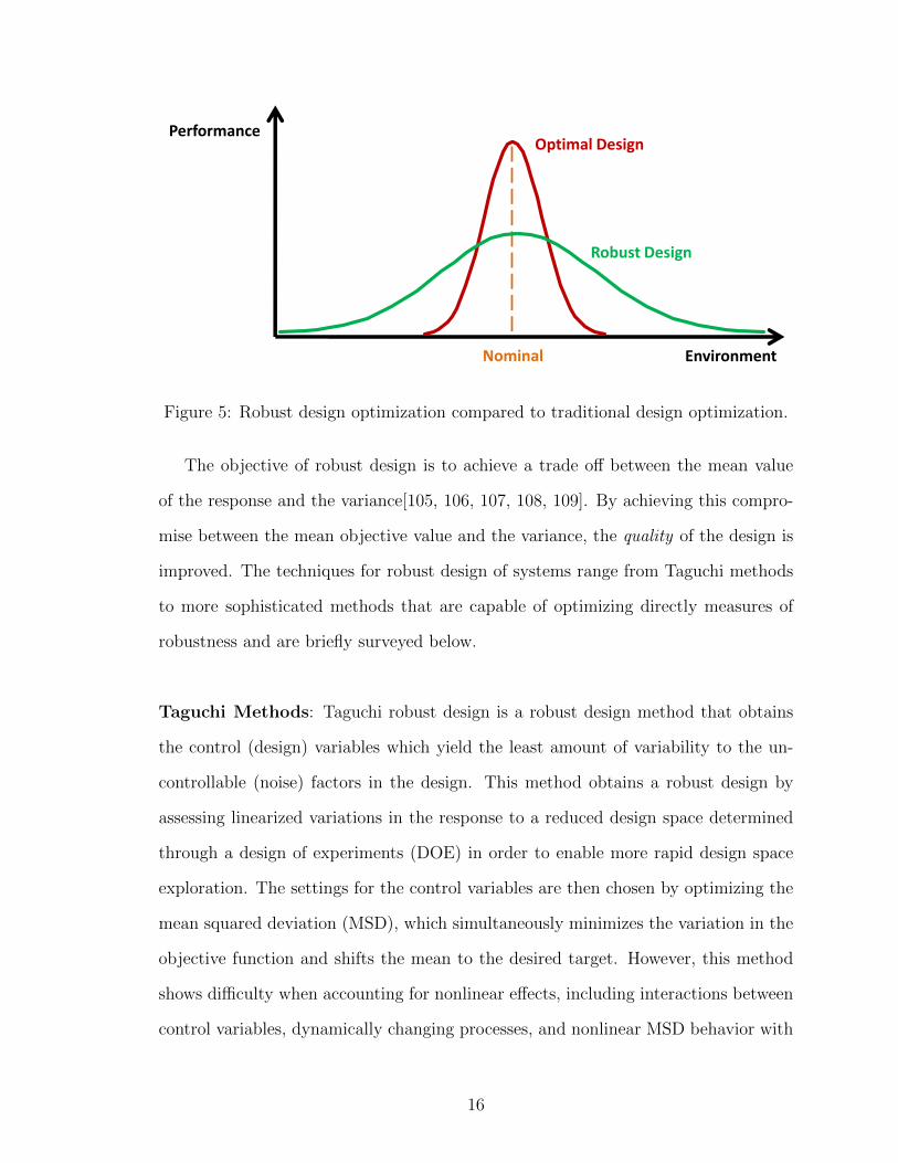
Figure 5: Robust design optimization compared to traditional design optimization.
The objective of robust design is to achieve a trade off between the mean value
of the response and the variance[105, 106, 107, 108, 109]. By achieving this compro-
mise between the mean objective value and the variance, the quality of the design is
improved. The techniques for robust design of systems range from Taguchi methods
to more sophisticated methods that are capable of optimizing directly measures of
robustness and are briefly surveyed below.
Taguchi Methods: Taguchi robust design is a robust design method that obtains
the control (design) variables which yield the least amount of variability to the un-
controllable (noise) factors in the design. This method obtains a robust design by
assessing linearized variations in the response to a reduced design space determined
through a design of experiments (DOE) in order to enable more rapid design space
exploration. The settings for the control variables are then chosen by optimizing the
mean squared deviation (MSD), which simultaneously minimizes the variation in the
objective function and shifts the mean to the desired target. However, this method
shows difficulty when accounting for nonlinear effects, including interactions between
control variables, dynamically changing processes, and nonlinear MSD behavior with
16
control variables. In addition, it only provides a relative measure of robustness rather
than an absolute measure and cannot be compared between designs and does not
account directly for design constraints[110, 104, 111, 112].
Nonlinear Programming Methods: Other robust design methods use traditional
optimization methods in a direct way. In particular, they use nonlinear programming
(NLP) methods to formulate the design problem. As opposed to Taguchi methods,
these methods are able to directly consider the constraints within the design. Several
different objective functions are usually considered. One is an objective function that
is a linear combination of the mean response and the spread of the response such as
that shown in Eq. (3).
J (u,p) = αµr(u,p) + βσr(u,p) (3)
In Eq. (3), α and β are scaling factors or weights, µr is the mean response, and σr
is the standard deviation of the response. Another formulation is in terms of the
feasibility. In this case, the objective function is given by
J (u,p) = P [gi(u,p) ≤ 0 | hj(u,p) = 0] =
∫gi(u,p)≤0hj(u,p)=0
fup(u,p)dudp (4)
where fup(u,p) is the joint probability density function of u and p.
Practically, obtaining the statistical quantities needed in these objectives (i.e.,
µr, σr, or fup(u,p)) analytically is unlikely. Therefore, the majority of techniques
in the literature obtain them by using a sampling method[113, 114, 104, 115]. The
downside to this approach is that it can be computationally intractable to optimize
on a statistically relevant sample if the function evaluation cost is significant.
One way to reduce the computational cost is by using approximation techniques
for the response of the design using a metamodel such as an RSE[116, 117, 118, 119].
17
However, approximating a complex design space using simplified models can be diffi-
cult. Another method for robust design when it is important to identify the feasibility
of a design is the extreme condition approach developed by Du and Chen[85]. This
approach derives the range of responses by min-max optimizations of the ranges of
the input and model uncertainties and then uses the results to find the optimum set
of design variables.
Non-statistical Methods: Not all techniques for robust design rely on comput-
ing the statistics of the design’s response. Some of these include worst case anal-
ysis, corner space analysis, and variation patterns. Worst case analysis assumes
that all of the system’s uncertainties can occur simultaneously in the worst possible
combination[120]. The effect on the constraint functions are then estimated based
on a Taylor series expansion and this is used to determine the feasibility of the de-
sign. Corner space evaluation is a similar concept; however, the variation in design
variables and parameters are not used to evaluate the variations in constraints[105].
Instead, a corner space is defined which consists of the vertices of the space defined
by the designs close to the target design point when perturbed under uncertainties.
Robust designs are then found by ensuring that the corner space touches the original
design constraints. Finally, variation patterns exploits the fact that uncertainties may
be correlated with each other and is a geometrical technique that identifies robust
designs at a given confidence level[121]. The shape of the design variable distribu-
tion, or pattern, is determined by their distribution and the size is determined by the
confidence level. For regular shapes, this allows rapid searching of robust designs;
however, for irregular shapes, the search can be computationally difficult.
18
1.2.4 Robust Multidisciplinary Design
The concept of robust multidisciplinary design is relatively new and few authors dis-
cuss accounting for uncertainties in this context. Work by Gu et al. attempt to
address this topic by representing model uncertainty as a bias to the system output
and applying the concept of worst case analysis combined with sensitivity analysis
to obtain a robust design[122, 123, 119]. This method, to date, fails to account for
generic uncertain parameter representations and model error estimation. Du and
Chen developed two different techniques to perform robustness analysis and design of
multidisciplinary systems, system uncertainty analysis (SUA) and concurrent subsys-
tem uncertainty analysis (CSSUA)[124, 125]. These techniques borrow concepts from
system sensitivity analysis at both the the local and global level in order to guide the
multidisciplinary design process.
System Uncertainty Analysis: SUA uses the mean values of the inputs to deter-
mine the mean values of the coupling variables and CA outputs. The mean values are
then used to obtain first-order Taylor series approximations for the outputs of each
CA which are then used to formulate a linear representation of the entire multidisci-
plinary design’s response. Since the response obtained is linear, uncertainty can be
propagated analytically to obtain the mean and variance of the design’s response.
Concurrent System Uncertainty Analysis: CSSUA parallelizes the assessment
of the variances in SUA. In order to achieve this parallel process, optimization is used
to find the mean of each CA output by targeting the mean value of each of the coupling
variables. Once these are found, the mean value of the design’s response can be found
by substituting the mean of the coupling variable with the sub-optimization result.
Finally the same technique from SUA is used to obtain the linear representation of
the multidisciplinary design’s robustness.
19
1.3 Dynamical Systems
A dynamical system uses a fixed rule to describe the evolution of a state. There are
two components of a dynamical system, a state vector which provides the state of the
system and a function which is the fixed rule describing how the state will evolve.
Definition: Dynamical System
Dynamical systems are functional relationships where a fixed rule describes howa state evolves. It requires:
1. A state variable (or vector) which characterizes the system
2. A fixed rule describing how the state changes
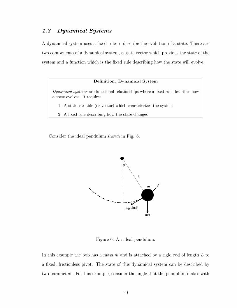
Consider the ideal pendulum shown in Fig. 6.
m
mg
sinmg
L
Figure 6: An ideal pendulum.
In this example the bob has a mass m and is attached by a rigid rod of length L to
a fixed, frictionless pivot. The state of this dynamical system can be described by
two parameters. For this example, consider the angle that the pendulum makes with
20
the vertical and the rotation rate of the pendulum recognizing there are other states
that could be used to describe the bob’s motion, such as its horizontal and vertical
position. Since gravity pulls the bob down with a force mg, it can be resolved into
two components: one which acts parallel to the rod and one which acts perpendicular.
Only the second affects the motion of the system. Applying Newton’s Second Law
for a constant mass, an equation in terms of θ, the angle the pendulum makes with
the vertical and the other parameters of the problem is able to be obtained:
θ = − gL
sin θ
This can be reduced to a first order system by making the substitution, x1 = θ and
x2 = θ. With a (state) vector denoted as x = (x1 x2)T , the first-order system is given
by
x =
x1
x2
= f(x) =
x2
− gL
sinx1
Where, from the definition of x1 and x2, the state variables are explicit in the fixed rule
since x1 = θ, the angular position of the pendulum with respect to the vertical, and
x2 = θ, the rotation rate of the pendulum are seen in the function f(x). Therefore,
since the pendulum has (1) a defined state and (2) a fixed rule describing the evolution
of the state, it is a dynamical system.
As another example of a dynamical system, consider the amount of money in a
bank account. Suppose that the annual interest rate, compounded monthly, is given
by r, then the account balance increases by a factor of (1 + r/12) each month. In
addition, suppose that a deposit, d, is made every month. In this example, the state,
x, is the balance in the account every month. The balance at month k+ 1 is given by
xk+1 =(
1 +r
12
)xk + d
Even though this relationship is given by a discrete, difference relationship, it has
both of the components required by a dynamical system: (1) a state and (2) a rule
21
describing the evolution of the state. Thus, the amount of money in a bank account
can be considered a dynamical system.
Finally, consider finding the root of a function g(x). The root is the value of x
such that the function’s value is 0. Many numerical methods for finding the root of a
function are dynamical systems since they rely on iterative schemes to identify the root
[126]. For instance, the bisection method, secant method, function iteration method,
and Newton’s method are all iterative techniques that satisfy the requirements of a
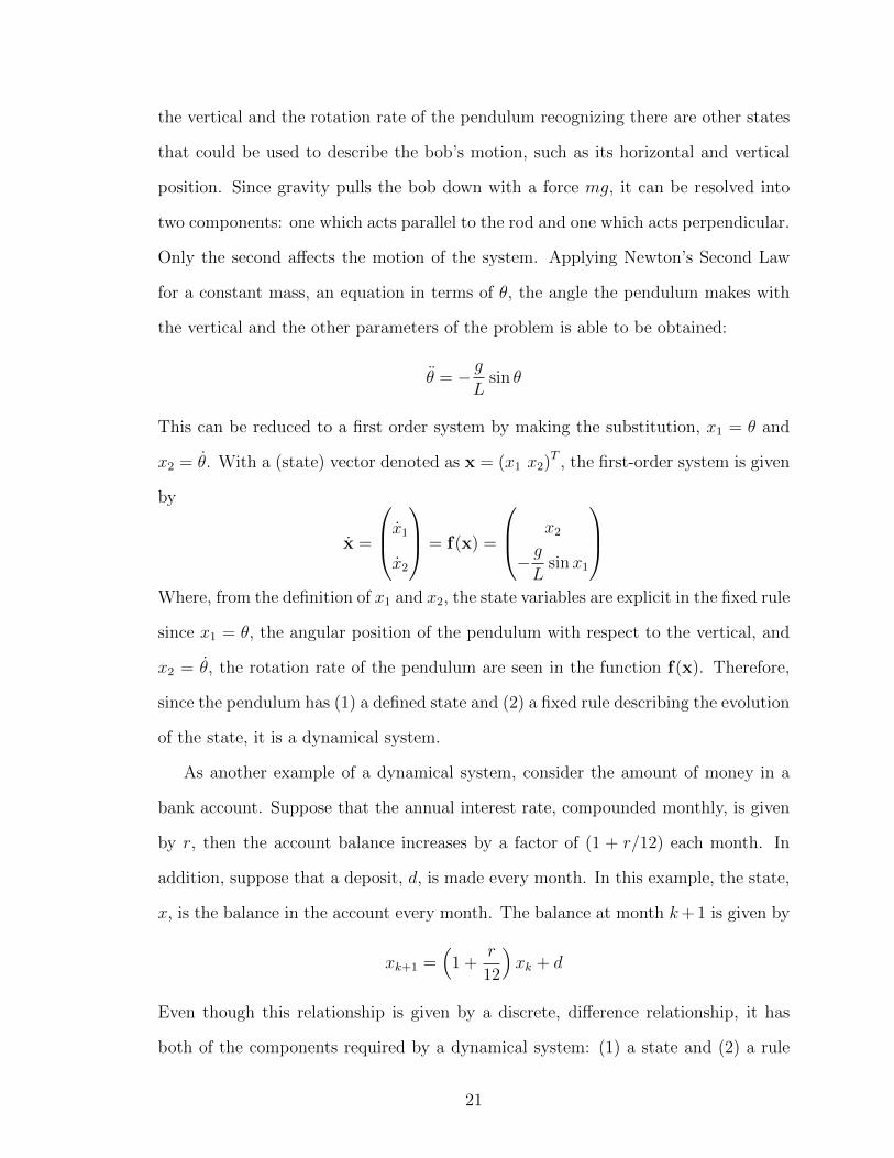
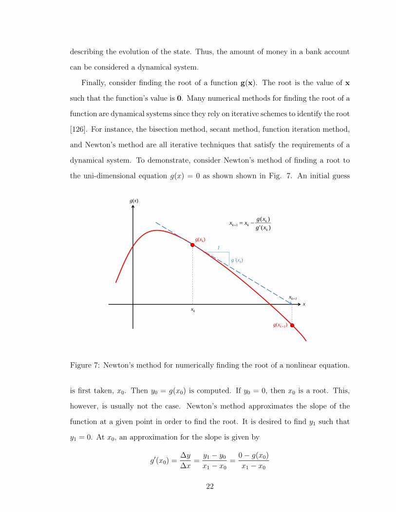
dynamical system. To demonstrate, consider Newton’s method of finding a root to
the uni-dimensional equation g(x) = 0 as shown shown in Fig. 7. An initial guess
g(x)
x xk
xk+1
g(xk)
g’(xk)
1
g(xk+1)
)('
)(1
k
kkk
xg
xgxx
Figure 7: Newton’s method for numerically finding the root of a nonlinear equation.
is first taken, x0. Then y0 = g(x0) is computed. If y0 = 0, then x0 is a root. This,
however, is usually not the case. Newton’s method approximates the slope of the
function at a given point in order to find the root. It is desired to find y1 such that
y1 = 0. At x0, an approximation for the slope is given by
g′(x0) =∆y
∆x=y1 − y0
x1 − x0
=0− g(x0)
x1 − x0
22
When this relationship is rearranged for x1 the following results
x1 = x0 −g(x0)
g′(x0)
This can be generalized for any iterate k
xk+1 = xk −g(xk)
g′(xk)
This relationship has the necessary components to be a dynamical system: (1) a state,
in this case x, and (2) a fixed rule describing how x evolves with iteration.
1.4 Previous Use of Dynamical System Concepts in Mul-tidisciplinary Design
Several investigators have applied concepts from dynamical systems in analyzing and
designing complex multidisciplinary systems.
One example which couples dynamical system concepts with multidisciplinary
design is given by Appa and Argyris in Ref. [127]. They use dynamical system
theory to simultaneously optimize the structure and trajectory of an aircraft. System
identification is used to characterize in a generalized state the nonlinear CAs of the
system using regression or neural network methods. The derivatives of the dynamic
properties of the aircraft can also be found using system identification. These are
then coupled with the dynamic equations of motion for the system in order to form
a functional in terms of the physical state variable and the generalized states. While
their work embraces multiple aspects of dynamical systems theory and satisfies the
definition of a dynamical system as they define both a state and how that state evolves,
they provide little detail on how they transformed the original problem into the state
space and their solution methods. Furthermore, their work requires that the design
variables appear explicitly in the modeling of the CAs for the system, (i.e., where
the model is given by f(u,p) instead of f(g(u),p)). This functional form prohibits
coupling between CAs and is therefore limited in the set of applicable problems.
23
Smith and Eppinger use stability concepts in the organization of a multidisci-
plinary design process[128]. Their work decomposes a DSM using eigenvectors in
order to minimize the feedback within the design. In this representation each of the
links between CAs is given a relative strength for the connection. Then the “modes”
are analyzed to identify the strongest connection. Although not explicitly described
in their work, by performing a modal analysis on the organization structure, an im-
plicit state is assumed, that of the information communicated between each of the
CAs. This state concept is identical to that used in this work. A similar organiza-
tional decomposition was made using game theory ideas by Lewis and Mistree[129].
This work iteratively anticipates the dependence of each CA on another and uses
that information to decompose the design for CAs that are lightly dependent on each
other. This work defines a state as the dependency of each CA on each other.
Others have combined an explicit dynamical system—that of the trajectory of a
vehicle—with multidisciplinary design. For instance, Delaurentis developed a method-
ology that probabilistically designed a multidisciplinary system at multiple levels of
the DSM hierarchy[41]. In this work, he employed metamodeling techniques for re-
sponse surface equations to design a vehicle in order to achieve a system level objec-
tive that includes both performance objectives (e.g., range and stability) and system
level considerations (e.g., weight). The developed metamodels contain variables for
the control system that directly impact the vehicle’s dynamical equations of motion
which govern the performance of the aircraft. The vehicle’s performance as well as
other sizing and synthesis components are accounted for, making it a multidisci-
plinary design; however, the use of dynamical system theory is limited to designing
the control system of the aircraft through the explicit equations of motion.
Work by Grant uses optimal control theory in order to simultaneously design the
trajectory and vehicle geometry for an entry, descent, and landing system[130, 131].
This work exploits dynamical system theory fully, albeit for a specific system in which
24
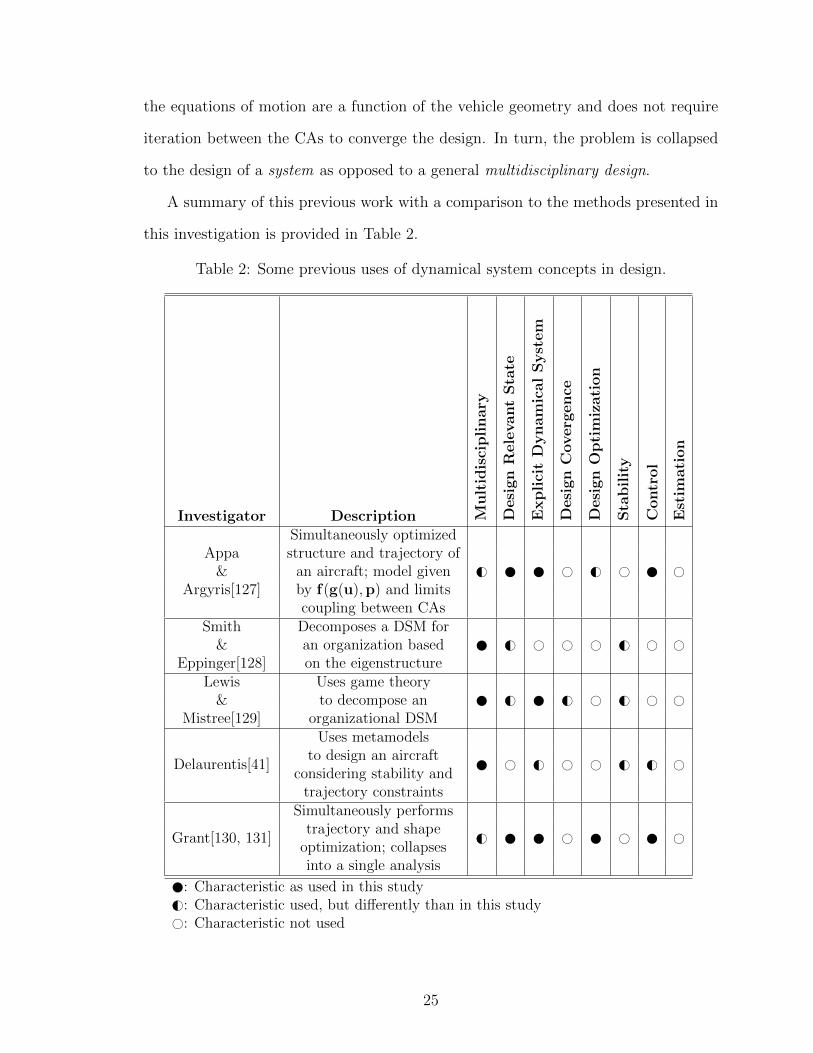
the equations of motion are a function of the vehicle geometry and does not require
iteration between the CAs to converge the design. In turn, the problem is collapsed
to the design of a system as opposed to a general multidisciplinary design.
A summary of this previous work with a comparison to the methods presented in
this investigation is provided in Table 2.
Table 2: Some previous uses of dynamical system concepts in design.
Investigator Description Mu
ltid
isci
pli
nary
Desi
gn
Rele
vant
Sta
te
Exp
lici
tD
yn
am
ical
Syst
em
Desi
gn
Coverg
en
ce
Desi
gn
Op
tim
izati
on
Sta
bil
ity
Contr
ol
Est
imati
on
Simultaneously optimized
G# # G# # #Appa structure and trajectory of
& an aircraft; model givenArgyris[127] by f(g(u),p) and limits
coupling between CAsSmith Decomposes a DSM for
G# # # # G# # #& an organization basedEppinger[128] on the eigenstructure
Lewis Uses game theory G# G# # G# # #& to decompose an
Mistree[129] organizational DSM
Delaurentis[41]
Uses metamodels
# G# # # G# G# #to design an aircraft
considering stability andtrajectory constraints
Grant[130, 131]
Simultaneously performs
G# # # #trajectory and shape
optimization; collapsesinto a single analysis
: Characteristic as used in this studyG#: Characteristic used, but differently than in this study#: Characteristic not used
25

1.5 Study Overview and Objectives
A general multidisciplinary design problem features coupling and feedback between
CAs. This feedback may lead to convergence issues requiring significant iteration in
order to obtain a feasible design.
Because finding a converged multidisciplinary design can be thought of as a multi-
dimensional root-finding problem, an iteration scheme can be developed for the state
vector, where the subsequent iteration relies on information from prior iterates. The
process of finding the root iteratively will be shown to be identical to the that of
solving a dynamical system. Therefore, the multidisciplinary design problem can be
cast as dynamical system where the state is the iteration-dependent data required
by each of the disciplines comprising the design. Casting the multidisciplinary de-
sign problem as dynamical system enables leveraging techniques associated with the
dynamical system field in order to overcome some of the traditional shortcomings of
multidisciplinary design techniques, such as the computational burden required by the
iteration and the potentially conflicting objectives between CA-level and system-level
optimizations.
Rigorous description for casting the multidisciplinary design problem as a dynami-
cal system, including handling of equality and inequality constraints within the design
will be provided. Three areas from dynamical system theory are chosen for detailed
investigation: stability analysis, optimal control, and estimation theory. Stability
analysis is used to investigate the existence of a solution to the design problem. This
analysis can be broadened to investigating the range of initial guesses that provide
guaranteed convergence for different iteration schemes. Optimal control techniques
allow the requirements associated with the design to be incorporated into the system
and allow for constraints that are functions of both the CA outputs and input values
to be handled simultaneously. Finally, estimation methods are employed to obtain
an evaluation of the robustness of the multidisciplinary design.
26
These three dynamical system techniques are then combined in a complete method-
ology for the rapid robust design of a linear multidisciplinary design. The developed
robust design methodology allows for uncertainties both within the models as well as
the parameters of the multidisciplinary problem. While linear multidisciplinary de-
signs are not common, extension to nonlinear designs is achievable through successive
linearization of the design or through an alternate estimation technique. A descrip-
tion of the appropriate domains of applicability for this linear technique is provided
in this thesis.
As observed in Table 2, this study is the only one to apply dynamical system theory
from the domains of stability, control, and estimation to the general multidisciplinary
design problem to address design convergence and optimization. In addition, it is the
only one to apply estimation theory to the quantify the uncertainty associated with
a design’s response.
1.6 Thesis Organization
The remaining portions of this thesis are organized as follows:
• Chapter 2 provides the theoretical context for this work. Included in this dis-
cussion is a definition of the state and discrete dynamical systems which enable
the casting of the multidisciplinary design problem in the form of a dynamical
system. In addition, the theoretical foundation for several other techniques uti-
lized within this work (e.g., root-finding methods, covariance matrices, matrix
norms, and unscented transform) are described. Finally, the chapter concludes
with a discussion of how to cast the multidisciplinary design problem as a dis-
crete dynamical system.
• Chapter 3 demonstrates how to apply various techniques from dynamical sys-
tem theory to the multidisciplinary design problem. These techniques include
using concepts from stability analysis, control theory, and estimation theory.
27
Stability analysis can be used to determine whether a design is feasible, whether
an optimal design exists, the range of initial values that can be used to converge
the design, and the rate at which the design will converge. Control theory is
able to be used to enforce constraints that are functions of the CA’s output and
the design variables at the same level in the optimization hierarchy. Finally,
techniques with roots in estimation theory can be used to propagate uncer-
tainty through the multidisciplinary design, leading to a way to simultaneously
converge the design and quantify the uncertainty associated with that design
point. For each of these dynamical system techniques, the theory underlying
their use is summarized followed by a discussion of how the technique can be
used in context of the multidisciplinary design problem.
• Chapter 4 integrates the techniques described in Chapter 3 into a rapid ro-
bust design methodology for linear multidisciplinary design which is capable of
extension to nonlinear multidisciplinary design through the use of successive
linearization. Within this chapter are formulations of the rapid robust de-
sign methodology using two root-finding techniques—fixed-point iteration and
Newton-Raphson iteration.
• Chapter 5 demonstrates each of the dynamical system techniques developed
in illustrative multidisciplinary design problems. This chapter pedagogically
progresses from relatively straight-forward analytical examples to more com-
plex practical examples. The chapter concludes with applying the developed
methodology to the design of a deployable aerodynamic surface for a strategic
system.
• Chapter 6 discusses the extensibility of the rapid robust design methodology
from both computational and accuracy perspectives. The effect of problem
scaling on computational cost is considered by examining the number of design
28

variables, number of CAs, nonlinearity of the CAs, and nonlinearity of the
response. In addition to computational cost, the accuracy of applying a method
with linear fundamentals to nonlinear problems is examined through nonlinear
perturbation analysis to identify the region of applicability for the method.
• Chapter 7 provides a summary of the thesis and its academic contributions.
In addition, various avenues for future work are discussed.
1.7 Academic Contributions
This thesis advances the state-of-the-art in the design and analysis of multidisciplinary
systems. The multidisciplinary design problem is recast as a dynamical system en-
abling new analyses to be performed and for a rapid robust design methodology to
be produced. The academic contributions of this research are summarized as follows:
Formulation of the General Multidisciplinary Design Problem as a Dynam-
ical System In Order to Leverage Established Techniques from Dynamical
System Theory
The convergence and optimization of a multidisciplinary design are root-finding prob-
lems, where the iterative techniques used to find the their solutions meet the require-
ments of a dynamical system. In turn, this allows the application of established
methods from dynamical systems to be applied to multidisciplinary design. Lever-
aging these techniques from dynamical system theory, the multidisciplinary design
process is shown to be more computationally tractable while yielding additional in-
sight into the problem.
29

Application of the Dynamical System Domain to the Multidisciplinary De-
sign Problem
The applicability of dynamical system techniques to the multidisciplinary design prob-
lem will be shown through application of three different areas—stability, control, and
estimation. These techniques are chosen for the speed and knowledge they provide
relative to traditional MDO techniques as well as their use in formulating a rapid
robust design methodology.
Stability Analysis : Stability theory provides insight into the existence of a design
based on the convergence procedure being utilized. For linear, constant coefficient
systems, stability can be checked through eigenanalysis. For more general designs,
the existence of a converged design can be identified through Lyapunov techniques.
Lyapunov techniques can also identify domains for which initial guesses result in con-
verged designs as well as to assess information regarding the rate of convergence.
Control Theory : Optimal control techniques allow constraints that are a function of
both the CA output and the design variables to be included at the same level of the
design hierarchy. This is a departure from many traditional MDO techniques, where
only constraints that are an explicit function of the design variables are considered.
By allowing for both types of constraints to be considered simultaneously, a coordi-
nated search of potential designs ensues which is capable of providing computational
efficiency.
Estimation Techniques : Estimation theory provides a means to obtain a rapid es-
timate of the mean and variance of the design. These estimates are provided by
propagating additional equations alongside the convergence relations. Furthermore,
design decomposition can be guided through the use of these techniques.
30

Development of a Linear Technique for the Rapid Robust Design of a Mul-
tidisciplinary System
Integrating these three areas of dynamical system theory together, a procedure for the
rapid robust design of a linear multidisciplinary system is produced. This methodol-
ogy provides a bound on the variance through the use of the matrix two-norm and is
applicable to nonlinear designs through successive linearization. The domain of appli-
cability of this rapid robust design methodology is quantified with respect to design
complexity, including nonlinearity. This design methodology is also demonstrated on
a suite of analytical and practical test problems.
Application of the Multidisciplinary Design Methodology to a Design Ex-
ample of Relevance to the Entry, Descent, and Landing Community
In addition to other test problems, a design example which obtains robust designs for
a deployable device that either increases the range or accuracy of a strategic system
is provided. This design example considers both the design of the deployable as well
as the selection of a guidance algorithm with comparisons to a contemporary robust
design methodology.
31
CHAPTER II
CASTING THE MULTIDISCIPLINARY DESIGN
PROBLEM AS A DYNAMICAL SYSTEM
This chapter provides the theoretical background for casting the multidisciplinary
design problem as a dynamical system beginning with a discussion of the enabling
theoretical foundations. These include a rigorous definition of the state and a dis-
crete dynamical system. This is followed by a mathematical description of several
numerical root-finding schemes and how each satisfies the criterion to be dynamical
system. Theoretical foundations for several other techniques utilized within this work
are then discussed including the covariance matrix, matrix norms, and a more rigor-
ous discussion of various methods for propagating uncertainty through mathematical
mappings. The chapter then concludes with a discussion of how to cast the multidis-
ciplinary design problem as a nested discrete dynamical system where feasible designs
are identified and then optimized.
2.1 Enabling Theoretical Foundations
2.1.1 The Concept of a State
The concept of a state is fundamental in transforming the multidisciplinary design
problem to a dynamical system. It is a summary of the status of the system at a
particular instance.
32

Definition: State
The state consists of the minimum set of parameters that completely summarizethe internal status of the dynamical system in the following sense: at any timet0 ∈ T the state x(t0) is known, then the output at a future instance in time,t1 ∈ T , y(t1) where t1 > t0 can be uniquely determined for a given evolutionscheme provided the input u[t0,t1] ∈ U is known.
In this work, two states will be considered—one which describes the output of
the CAs for the convergence of the design and another which describes the design
variables during the optimization of the design.
2.1.2 Mathematical Definition of a Dynamical System
Mathematically, a dynamical system is a set of times T , spaces U , Σ, and Y , and
transformations g : T ×T ×Σ×U → Σ and h : T ×Σ×U s → Y t. The transformations
g and h are such that[132]
x(t1) = g(t0, t1,x(t0),u[t0,t1])
and
y(t1) = h(t1,x(t1),u(t1))
The sextuple, (T ,U ,Σ,Y ,g,h), defines a dynamical system provided the transforma-
tions have the following properties:
1. Identity Property: for every t0, t1 ∈ T ,
x(t0) = g(t0, t0,x(t0), u[t0,t1])
2. State Transition Property: for every u ∈ U , v ∈ U such that u = v over an
interval [t0, t1] ∈ T , then
g(t0, t1,x(t0),u[t0,t1]) = g(t0, t1,x(t0),v[t0,t1])
33
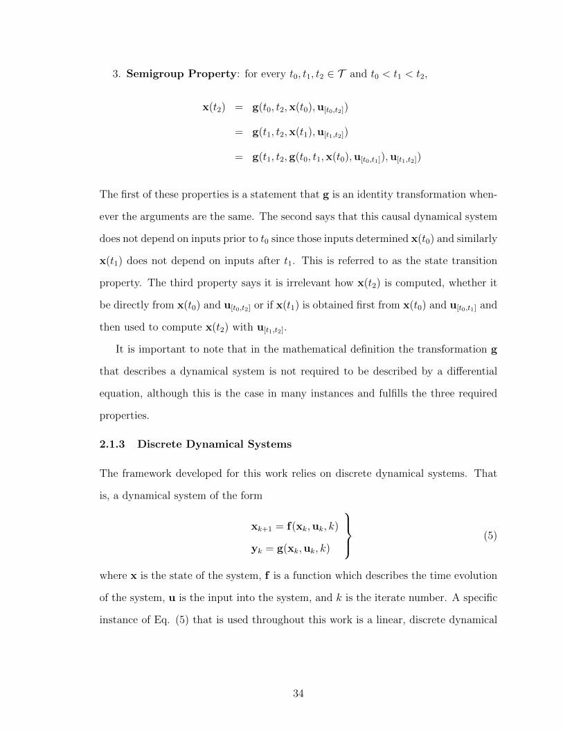
3. Semigroup Property: for every t0, t1, t2 ∈ T and t0 < t1 < t2,
x(t2) = g(t0, t2,x(t0),u[t0,t2])
= g(t1, t2,x(t1),u[t1,t2])
= g(t1, t2,g(t0, t1,x(t0),u[t0,t1]),u[t1,t2])
The first of these properties is a statement that g is an identity transformation when-
ever the arguments are the same. The second says that this causal dynamical system
does not depend on inputs prior to t0 since those inputs determined x(t0) and similarly
x(t1) does not depend on inputs after t1. This is referred to as the state transition
property. The third property says it is irrelevant how x(t2) is computed, whether it
be directly from x(t0) and u[t0,t2] or if x(t1) is obtained first from x(t0) and u[t0,t1] and
then used to compute x(t2) with u[t1,t2].
It is important to note that in the mathematical definition the transformation g
that describes a dynamical system is not required to be described by a differential
equation, although this is the case in many instances and fulfills the three required
properties.
2.1.3 Discrete Dynamical Systems
The framework developed for this work relies on discrete dynamical systems. That
is, a dynamical system of the form
xk+1 = f(xk,uk, k)
yk = g(xk,uk, k)
(5)
where x is the state of the system, f is a function which describes the time evolution
of the system, u is the input into the system, and k is the iterate number. A specific
instance of Eq. (5) that is used throughout this work is a linear, discrete dynamical
34
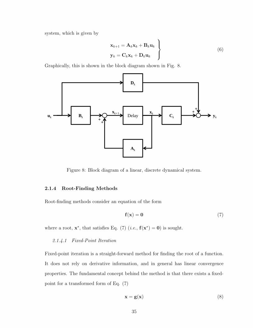
system, which is given by
xk+1 = Akxk + Bkuk
yk = Ckxk + Dkuk
(6)
Graphically, this is shown in the block diagram shown in Fig. 8.
Bk Ck
Ak
Dk
Delay uk yk
xk xk+1
+ +
+ +
Figure 8: Block diagram of a linear, discrete dynamical system.
2.1.4 Root-Finding Methods
Root-finding methods consider an equation of the form
f(x) = 0 (7)
where a root, x∗, that satisfies Eq. (7) (i.e., f(x∗) = 0) is sought.
2.1.4.1 Fixed-Point Iteration
Fixed-point iteration is a straight-forward method for finding the root of a function.
It does not rely on derivative information, and in general has linear convergence
properties. The fundamental concept behind the method is that there exists a fixed-
point for a transformed form of Eq. (7)
x = g(x) (8)
35
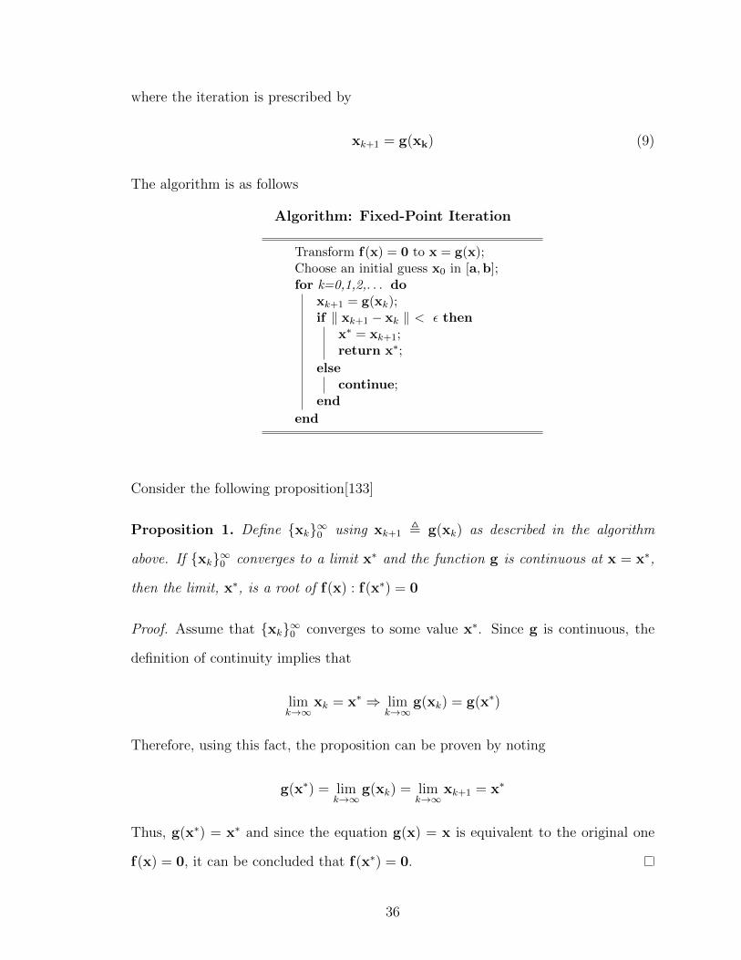
where the iteration is prescribed by
xk+1 = g(xk) (9)
The algorithm is as follows
Algorithm: Fixed-Point Iteration
Transform f(x) = 0 to x = g(x);Choose an initial guess x0 in [a,b];for k=0,1,2,. . . do
xk+1 = g(xk);if ‖ xk+1 − xk ‖ < ε then
x∗ = xk+1;return x∗;
elsecontinue;
end
end
Consider the following proposition[133]
Proposition 1. Define xk∞0 using xk+1 , g(xk) as described in the algorithm
above. If xk∞0 converges to a limit x∗ and the function g is continuous at x = x∗,
then the limit, x∗, is a root of f(x) : f(x∗) = 0
Proof. Assume that xk∞0 converges to some value x∗. Since g is continuous, the
definition of continuity implies that
limk→∞
xk = x∗ ⇒ limk→∞
g(xk) = g(x∗)
Therefore, using this fact, the proposition can be proven by noting
g(x∗) = limk→∞
g(xk) = limk→∞
xk+1 = x∗
Thus, g(x∗) = x∗ and since the equation g(x) = x is equivalent to the original one
f(x) = 0, it can be concluded that f(x∗) = 0.
36
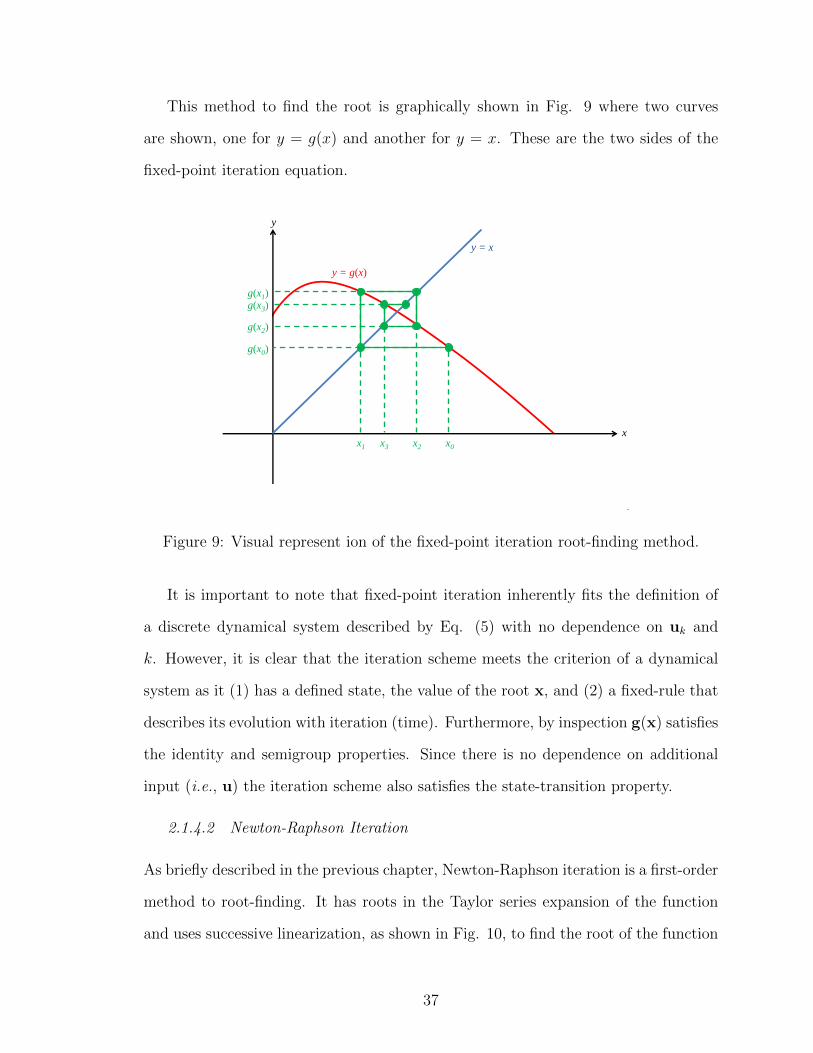
This method to find the root is graphically shown in Fig. 9 where two curves
are shown, one for y = g(x) and another for y = x. These are the two sides of the
fixed-point iteration equation.
x x0 x2 x3 x1
g(x0)
g(x2)
g(x3) g(x1)
y = x
y = g(x)
y
Figure 9: Visual represent ion of the fixed-point iteration root-finding method.
It is important to note that fixed-point iteration inherently fits the definition of
a discrete dynamical system described by Eq. (5) with no dependence on uk and
k. However, it is clear that the iteration scheme meets the criterion of a dynamical
system as it (1) has a defined state, the value of the root x, and (2) a fixed-rule that
describes its evolution with iteration (time). Furthermore, by inspection g(x) satisfies
the identity and semigroup properties. Since there is no dependence on additional
input (i.e., u) the iteration scheme also satisfies the state-transition property.
2.1.4.2 Newton-Raphson Iteration
As briefly described in the previous chapter, Newton-Raphson iteration is a first-order
method to root-finding. It has roots in the Taylor series expansion of the function
and uses successive linearization, as shown in Fig. 10, to find the root of the function
37
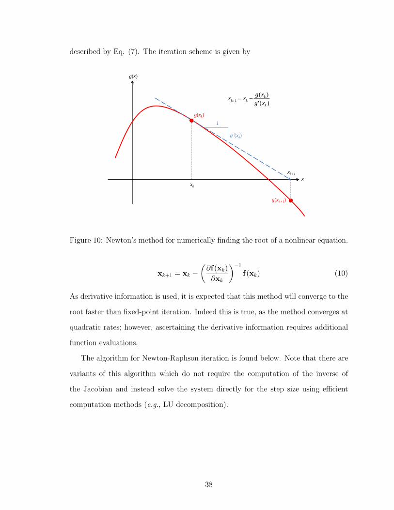
described by Eq. (7). The iteration scheme is given by
g(x)
x xk
xk+1
g(xk)
g’(xk)
1
g(xk+1)
)('
)(1
k
kkk
xg
xgxx
Figure 10: Newton’s method for numerically finding the root of a nonlinear equation.
xk+1 = xk −(∂f(xk)
∂xk
)−1
f(xk) (10)
As derivative information is used, it is expected that this method will converge to the
root faster than fixed-point iteration. Indeed this is true, as the method converges at
quadratic rates; however, ascertaining the derivative information requires additional
function evaluations.
The algorithm for Newton-Raphson iteration is found below. Note that there are
variants of this algorithm which do not require the computation of the inverse of
the Jacobian and instead solve the system directly for the step size using efficient
computation methods (e.g., LU decomposition).
38
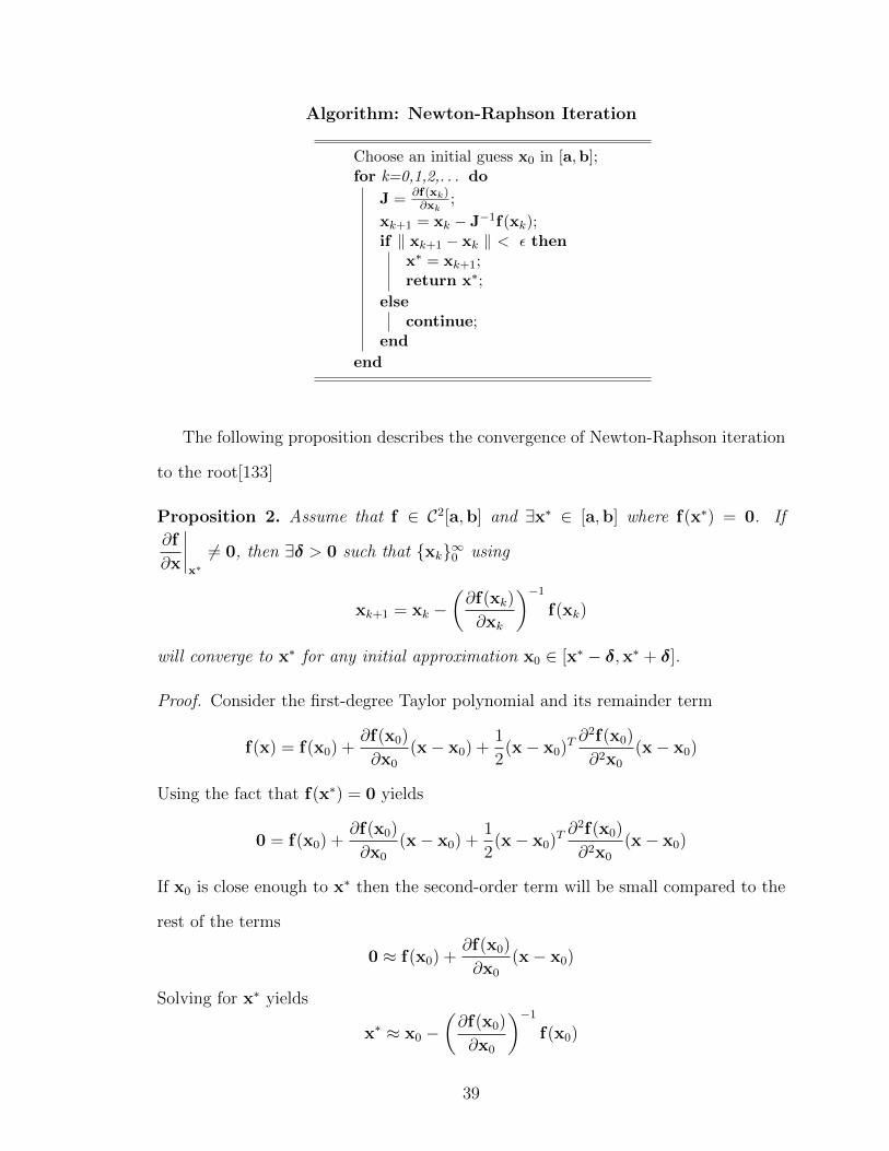
Algorithm: Newton-Raphson Iteration
Choose an initial guess x0 in [a,b];for k=0,1,2,. . . do
J = ∂f(xk)∂xk
;
xk+1 = xk − J−1f(xk);if ‖ xk+1 − xk ‖ < ε then
x∗ = xk+1;return x∗;
elsecontinue;
end
end
The following proposition describes the convergence of Newton-Raphson iteration
to the root[133]
Proposition 2. Assume that f ∈ C2[a,b] and ∃x∗ ∈ [a,b] where f(x∗) = 0. If
∂f
∂x
∣∣∣∣x∗6= 0, then ∃δ > 0 such that xk∞0 using
xk+1 = xk −(∂f(xk)
∂xk
)−1
f(xk)
will converge to x∗ for any initial approximation x0 ∈ [x∗ − δ,x∗ + δ].
Proof. Consider the first-degree Taylor polynomial and its remainder term
f(x) = f(x0) +∂f(x0)
∂x0
(x− x0) +1
2(x− x0)T
∂2f(x0)
∂2x0
(x− x0)
Using the fact that f(x∗) = 0 yields
0 = f(x0) +∂f(x0)
∂x0
(x− x0) +1
2(x− x0)T
∂2f(x0)
∂2x0
(x− x0)
If x0 is close enough to x∗ then the second-order term will be small compared to the
rest of the terms
0 ≈ f(x0) +∂f(x0)
∂x0
(x− x0)
Solving for x∗ yields
x∗ ≈ x0 −(∂f(x0)
∂x0
)−1
f(x0)
39

which can be used to define the next approximation, x1 to the root
x1 = x0 −(∂f(x0)
∂x0
)−1
f(x0)
which leads to the general rule
xk+1 = xk −(∂f(xk)
∂xk
)−1
f(xk)
Note that this general recursive relation is analogous to the fixed-point relation xk+1 =
g(xk). It can be shown that
∂g(x)
∂x= I−
(∂f(x)
∂x
)−T [∂f(x)
∂x
∂f(x)
∂x− ∂2f(x)
∂2xf(x)
](∂f(x)
∂x
)−1
=
(∂f(x)
∂x
)−T [∂2f(x)
∂2xf(x)
](∂f(x)
∂x
)−1
By hypothesis, f(x∗) = 0 and therefore∂g(x∗)
∂x∗= 0. Because
∂g(x∗)
∂x∗= 0 and g(x)
is continuous it is possible to find a δ > 0 so that ‖ ∂g(x)
∂x‖< 1 is satisfied on
[x∗ − δ,x∗ + δ]. Therefore, the sequence xk∞0 converges to the root x = x∗ for
x0 ∈ [x∗ − δ,x∗ + δ]
The next iterate of Newton-Raphson iteration is only a function of the current
iterate, xk, therefore it forms a discrete dynamical system as described in Eq. (5)
with no dependence on uk and k. Therefore, as with fixed-point iteration, it can also
be shown that Newton-Raphson iteration meets the mathematical requirements of a
dynamical system.
2.1.5 The Covariance Matrix
The covariance matrix of a n-dimensional random vector X is an n×n matrix defined
as follow[59]
Σ = E[(X− E[X]) (X− E[X])T
](11)
and can be thought of as a generalization of the scalar variance of a single random
variable X with mean µ and variance σ2 = E[(X − µ)2]. Note that the covariance
40
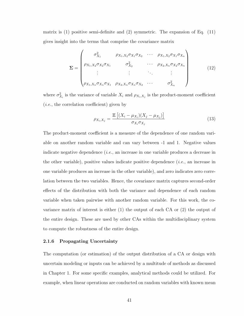
matrix is (1) positive semi-definite and (2) symmetric. The expansion of Eq. (11)
gives insight into the terms that comprise the covariance matrix
Σ =
σ2X1
ρX1,X2σX1σX2 · · · ρX1,X2σX1σXn
ρX1,X2σX2σX1 σ2X2
· · · ρX2,XnσX2σXn
......
. . ....
ρX1,XnσXnσX1 ρX2,XnσXnσX2 · · · σ2Xn
(12)
where σ2Xi
is the variance of variable Xi and ρXi,Xjis the product-moment coefficient
(i.e., the correlation coefficient) given by
ρXi,Xj=
E[(Xi − µXi
)(Xj − µXj)]
σXiσXj
(13)
The product-moment coefficient is a measure of the dependence of one random vari-
able on another random variable and can vary between -1 and 1. Negative values
indicate negative dependence (i.e., an increase in one variable produces a decrease in
the other variable), positive values indicate positive dependence (i.e., an increase in
one variable produces an increase in the other variable), and zero indicates zero corre-
lation between the two variables. Hence, the covariance matrix captures second-order
effects of the distribution with both the variance and dependence of each random
variable when taken pairwise with another random variable. For this work, the co-
variance matrix of interest is either (1) the output of each CA or (2) the output of
the entire design. These are used by other CAs within the multidisciplinary system
to compute the robustness of the entire design.
2.1.6 Propagating Uncertainty
The computation (or estimation) of the output distribution of a CA or design with
uncertain modeling or inputs can be achieved by a multitude of methods as discussed
in Chapter 1. For some specific examples, analytical methods could be utilized. For
example, when linear operations are conducted on random variables with known mean
41
and covariance an exact propagation of the uncertainty is possible[59]. However, in
general, approximate techniques must be used. In this work, a sampling method,
the unscented transform, is pursued. The unscented transform selects the samples
so that the moments of the probability distribution can be matched. This leads
to more accurate estimates of the probability distributions. In addition, once the
multidisciplinary design is formulated as a dynamical system, covariance techniques
which implement a Kalman filter can be invoked as shown in Chapter 3.
While the theoretical development of the method in this investigation considers
all analyses to be linear (or linearized) such that an analytic propagation is possible,
the formulation discussed later allows extension to nonlinear applications.
2.1.6.1 Sample Statistics
Sample statistics describe the statistics of a known set of values. In this methodology,
it can be assumed that the sample is the resultant of a number of propagated trials
through the analysis. There are two two sample statistics of interest: the sample
mean (x) and the sample covariance (S). The unbiased estimates of each of these is
given by Eqs. (14) and (15), respectively[59].
x =1
n
n∑i=1
xi (14)
Sjk =1
n− 1
n∑i=1
(xij − xj)(xik − xk) (15)
2.1.6.2 The Unscented Transform
The unscented transform approximates a probability distribution by selecting a small
number of test points, the sigma points, which are propagated through the analysis
to allow estimation of the posterior mean and covariance. While this is similar to
Monte Carlo analysis because a trial is propagated through the analysis, by selecting
the test points according to the eigenstructure of the covariance matrix, third-order
42
accurate estimates of the resulting distribution’s mean and covariance matrix are
achievable with a small number of sigma points[134]. The relative speed and accuracy
of computation for the uncertainty propagation leads this technique to be the basis
of the Unscented Kalman Filter[135].
Conceptually, the unscented transform can be understood through the follow-
ing development. Suppose that the output of an analysis, y, is related to the n-
dimensional input, x, by the relationship
y = g(x) (16)
where x has mean x and covariance Σ. The set of trial points are selected based on
the solution of the relationship[134]
AAT = nΣ (17)
There are an infinite number of matrices, A, that satisfy Eq. (17). Two commonly
used solutions are the upper triangular matrix found from the Cholesky decomposition
and the symmetric square root matrix. A set of 2n points, S = σi2ni=1, are then
selected as the columns of ±A. The set of trial points are then given by[134]
X i = σi + x (18)
and are propagated through the CA, Eq. (16)[134]
Y i = g(X i) (19)
. This set can then be used to find the mean and covariance matrix of the analysis’
output, which are given by[134]
y ≈ 1
2n
2n∑i=1
Y i (20)
Σ ≈ 1
2n
2n∑i=1
[Y i − y] [Y i − y]T (21)
43
These estimates are third-order accurate, meaning for analyses with polynomial input-
output relationships that are less than cubic, the approximation is exact. Hence, for
minimal computational expense (two times the function evaluations as the dimension-
ality of the matrix, A) a very good approximation of both the mean of the output of
the analysis (or design) and the output covariance matrix is obtained[134].
2.1.7 Matrix Norms
In order to obtain a singular value that bounds the variance, consider the matrix
two-norm which is defined as[136]
‖ A ‖2= max‖x‖2=1
‖ Ax ‖2=√λmax(AHA) (22)
where AH represents the conjugate transpose of a matrix A and λmax(·) is a function
which returns the maximum eigenvalue. The two-norm can be more readily under-
stood in the context of spectral decomposition such that D = V−1AV where D is at
worst a block-diagonal matrix. In the case of real, distinct eigenvalues, the diagonal
of matrix D consists of the eigenvalues. By virtue of the properties of the covari-
ance matrix, Σ, the maximum eigenvalue is greater than or equal to the maximum
variance. This means that the two-norm provides a bound on the maximum variance.
In two-dimensions, this can be seen in Fig. 11 where the covariance matrix is
plotted as an ellipse. In Fig. 11, the axes σX1σX2 are the standard deviations as-
sociated with the covariance matrix, Σ. The eigenvectors of the covariance matrix
form the alternate set of axes (in blue), σX′1σX′2 . The two-norm is the variance of
the “pseudo-variable” that is oriented along the principal eigenvector of the resulting
ellipse, which is the magnitude of the semi-major axis of the ellipse. In other words,
the two-norm is the radius of the circle which completely encompasses the covariance
matrix. An advantageous feature of this norm is that it is always a conservative
estimate of the variance of the system.
Another way to view the resulting bound is through the auxiliary circle that is
44

1X
2X
'1X
'2X
2Σ
Figure 11: Visual representation of the matrix two-norm.
formed from sweeping through the eccentric anomaly of an elliptical orbit. This
auxiliary circle completely encompasses the elliptical orbit and is coincident with the
orbit at two points (when the true anomaly is 0 and 180), much in the same way
that the two-norm encompasses the ellipse formed from a covariance matrix and is
coincident at two points.
2.2 Multidisciplinary Design as a Dynamical System
2.2.1 Identification of Feasible Designs
Identifying feasible designs in multidisciplinary systems can be thought of as the
process of finding the root of a function. Consider a multidisciplinary problem where
the analysis variables are described by a multivariable function f(u,p) where u are
the design variables and p are the parameters of the problem. Assume that the
requirements of the design are given by only equality constraints that are a function
of the performance of the system. The performance of the design is described by a
multivariable mapping g(f(u,p)) and the requirements are given by z. In order to
45
meet the requirements it is necessary to adjust the design variables u so that
z = g(f(u,p)) (23)
The solution u∗ of Eq. (23) is the root of the system. Since identifying feasible
designs within the multidisciplinary design problem requires finding the value of u
that satisfies Eq. (23), this process can be thought of as a root-finding problem when
an iterative solution method is chosen. As described previously, many of the iterative
schemes to find the root of a function, g(u), can be thought of as a dynamical system.
Therefore, finding the feasible designs can be a dynamical system.
2.2.2 Design Optimization
In order for a converged design to be an optimum with respect to some objective func-
tion, its performance needs to be evaluated with respect to other potential designs.
The general optimization problem is formulated as
Minimize: J (u,p)
Subject to: gi(u,p) ≤ 0, i = 1, . . . , ng
hj(u,p) = 0, j = 1, . . . , nh
By varying: u
(24)
which requires a stationary point of the Lagrangian given as
L(u,p,λ) = J (u,p) +
ng∑i=1
λigi(u,p) +
nh∑j=1
λng+jhj(u,p) (25)
to be found. The stationary point of the Lagrangian (Eq. (25)) is the value of u
such that ∇uL(u,p,λ) = 0. This is also a root-finding problem and therefore can be
thought of as a dynamical system.
2.2.3 Identifying an Optimal Multidisciplinary Design
Multidisciplinary design optimization can be broken down into two steps: (1) identi-
fying feasible designs and (2) identifying the optimal design from the set of feasible
46
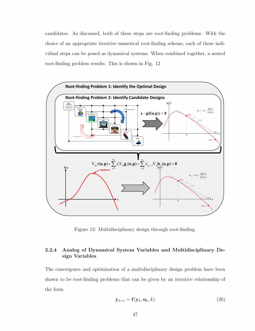
candidates. As discussed, both of these steps are root-finding problems. With the
choice of an appropriate iterative numerical root-finding scheme, each of these indi-
vidual steps can be posed as dynamical systems. When combined together, a nested
root-finding problem results. This is shown in Fig. 12
Root-finding Problem 2: Identify Candidate Designs
Root-finding Problem 1: Identify the Optimal Design
z - g(f(u,p)) = 0
0puhpugpu uuu
h
g
g n
j
jjn
n
i
ii
11
),(),(),( J
System Definition
Planetary Model
GN&C
Trajectory
Thermal
Sizing
Aerodynamics
Feedforward
Feedback
J(x)
x
Optimum
g(u)
uuk
uk+1
g(uk)
g’(uk)
1
g(uk+1)
)('
)(1
k
kkk
ug
uguu
g(u)
uuk
uk+1
g(uk)
g’(uk)
1
g(uk+1)
)('
)(1
k
kkk
ug
uguu
Figure 12: Multidisciplinary design through root-finding.
2.2.4 Analog of Dynamical System Variables and Multidisciplinary De-sign Variables
The convergence and optimization of a multidisciplinary design problem have been
shown to be root-finding problems that can be given by an iterative relationship of
the form
yk+1 = f(yk,uk, k) (26)
47
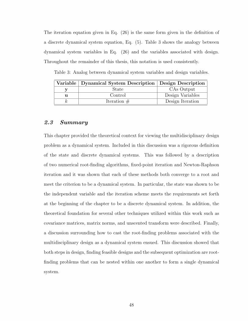
The iteration equation given in Eq. (26) is the same form given in the definition of
a discrete dynamical system equation, Eq. (5). Table 3 shows the analogy between
dynamical system variables in Eq. (26) and the variables associated with design.
Throughout the remainder of this thesis, this notation is used consistently.
Table 3: Analog between dynamical system variables and design variables.
Variable Dynamical System Description Design Descriptiony State CAs Outputu Control Design Variablesk Iteration # Design Iteration
2.3 Summary
This chapter provided the theoretical context for viewing the multidisciplinary design
problem as a dynamical system. Included in this discussion was a rigorous definition
of the state and discrete dynamical systems. This was followed by a description
of two numerical root-finding algorithms, fixed-point iteration and Newton-Raphson
iteration and it was shown that each of these methods both converge to a root and
meet the criterion to be a dynamical system. In particular, the state was shown to be
the independent variable and the iteration scheme meets the requirements set forth
at the beginning of the chapter to be a discrete dynamical system. In addition, the
theoretical foundation for several other techniques utilized within this work such as
covariance matrices, matrix norms, and unscented transform were described. Finally,
a discussion surrounding how to cast the root-finding problems associated with the
multidisciplinary design as a dynamical system ensued. This discussion showed that
both steps in design, finding feasible designs and the subsequent optimization are root-
finding problems that can be nested within one another to form a single dynamical
system.
48
CHAPTER III
APPLYING DYNAMICAL SYSTEM THEORY TO
MULTIDISCIPLINARY DESIGN
This chapter builds on the approach of casting the multidisciplinary design prob-
lem as a dynamical system shown in Chapter 2 to apply dynamical system theory.
Techniques from dynamical system theory are applied to the multidisciplinary design
problem, including concepts from stability analysis, control theory, and estimation
theory. Stability analysis is shown to be able to determine whether a design is feasi-
ble, whether an optimal design exists, the range of initial values that can be used to
converge the design, and the rate at which the design will converge. Control theory
enables efficient handling of constraints as it enforces constraints that are functions
of the CA’s output and the design variables at the same level in the optimization
hierarchy. Finally, estimation theory is used to propagate uncertainty through the
multidisciplinary design, yielding a method that simultaneously converges the design
and quantifies the uncertainty associated with that design point.
3.1 Design Convergence Using Stability Concepts
Concepts from the stability domain of dynamical system theory are applied to mul-
tidisciplinary design in order to identify:
1. Whether a feasible design exists (for a given iteration scheme)
2. Whether an optimal design exists (for a given iteration scheme)
3. The range of initial values that can be used to converge the design
4. The rate at which the design will converge
49
Each of these is an enhancement compared to current MDA/O techniques enabled by
viewing the iterative relationships formed in the convergence of the design problem
as a dynamical system.
3.1.1 Foundations of Stability Analysis
The concept of stability allows for the identification of feasible designs for given
iteration schemes. These iteration schemes can usually be written in the form
yk+1 = f(yk,uk) (27)
where y is the state of the system, f is a function which describes the time evolution
of the system, u is the input into the system, and k is the iterate number. A specific
instance of Eq. (27) is a linear, discrete dynamical system, which is given by
yk+1 = Akyk + Bkuk (28)
For a given initial state, a system is stable if the state does not grow beyond
the initial state’s magnitude. More rigorously, this is defined in terms of equilibrium
points of a system. Consider the discrete dynamical system defined by Eq. (27), the
equilibrium point is defined as
Definition: Equilibrium of a Dynamical System
A particular point ye is an equilibrium point of the dynamical system given byEq. (27) if the system’s state at iterate k = 0 is ye implies that ∀k ∈ Z+ \ 0,f(ye,0) = ye.
For a linear dynamical system, given by Eq. (28), the equilibrium point is the origin
of the system (i.e., ye = 0).
The equilibrium point’s stability is defined with regard to the zero-input discrete
50

dynamical system given by[132, 137, 138, 139]
yk+1 = f(yk,0)
yk=0 = y0
(29)
Definition: Stability
For the system given by Eq. (29), if ∀ε > 0, ∃δ(ε, 0) ∈ (0, ε] an equilibrium pointof the system is
• stable if ∀k > 0 and ‖ y0 ‖< δ, ‖ yk ‖< ε
• asymptotically stable if
1. the equilibrium point is stable and
2. ∃δ′ ∈ (0, ε] such that whenever ‖ y0 ‖< δ′ the state’s evolutionsatisfies lim
k→∞‖ yk ‖= 0
• unstable if it is not stable or asymptotically stable
Figures 13 and 14 demonstrate the concept of equilibrium point stability. Figure
13 shows an intuitive concept of stability while Fig. 14 demonstrates different state
trajectories in R2 × R and R2. In Fig. 14, asymptotically stable state trajectories
are seen to approach the origin as time progresses whereas stable trajectories remain
within a given distance, ε of the origin.
Asymptotically
Stable
Stable Unstable
Figure 13: Visualization of the concept of stability.
51
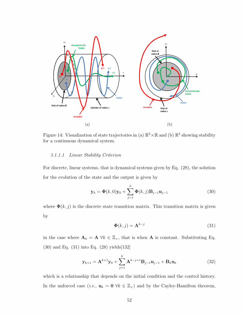
y0
y0
y0
y(t) y(t)
y(t) t
y1
y2
Stable
Unstable
Asymptotically Stable
Cylinder of radius ε Disk of radius
(a)
y2
y1
Asymptotically Stable
Stable
Unstable Disk of radius ε
Disk of radius
(b)
Figure 14: Visualization of state trajectories in (a) R2×R and (b) R2 showing stabilityfor a continuous dynamical system.
3.1.1.1 Linear Stability Criterion
For discrete, linear systems, that is dynamical systems given by Eq. (28), the solution
for the evolution of the state and the output is given by
yk = Φ(k, 0)y0 +k∑j=1
Φ(k, j)Bj−1uj−1 (30)
where Φ(k, j) is the discrete state transition matrix. This transition matrix is given
by
Φ(k, j) = Ak−j (31)
in the case where Ak = A ∀k ∈ Z+, that is when A is constant. Substituting Eq.
(30) and Eq. (31) into Eq. (28) yields[132]
yk+1 = Ak+1y0 +k∑j=1
Ak−j+1Bj−1uj−1 + Bkuk (32)
which is a relationship that depends on the initial condition and the control history.
In the unforced case (i.e., uk = 0 ∀k ∈ Z+) and by the Cayley-Hamilton theorem,
52
the stability criterion can be identified. If maxi|λi| > 1 for any simple root of the
characteristic equation
det(A− λI) = 0 (33)
or maxi|λi| ≥ 1 for any repeated root of Eq. (33) then the system is unstable. This
is because the Jordan canonical form of A has terms that tend to infinity as the
iteration proceeds (i.e., limk→∞
VTAkV =∞ since diagonal terms of VTAV are greater
than unity). Similarly, if maxi|λi| ≤ 1 for any simple root or max
i|λi| < 1 for repeated
roots of Eq. (33), then the iteration scheme is asymptotically stable[132, 140, 141].
More rigorous proof of this concept is provided in Ref. [140].
3.1.1.2 Lyapunov Stability
Stability of general dynamical systems, including the one formed for design, can be
studied using Lyapunov stability theory. This theory lays the foundations to assess the
stability characteristics of arbitrary designs and can be leveraged to provide insight
about the convergence properties of the design. For instance, Lyapunov stability can
be used to ascertain information regarding the convergence rate and what starting
iteration values will lead to a converged design for a given root-finding scheme.
Lyapunov stability theory is prevalent for continuous dynamical systems such as
the autonomous system
y = f(y), ∀t ∈ [0,∞) (34)
for which the origin is an equilibrium point. A Lyapunov function is a continuously
differentiable map V : Rn → R such that
1. V (y) > 0, y 6= 0, V (0) = 0
2.d
dt(V (y(t))) ≤ 0, ∀t ∈ [0,∞)
where y : [0,∞)→ Rn is any solution of Eq. (34)[138]. In fact, it has been applied to
differential equations such as this since Lyapunov first defined this technique in 1892.
53
Its use in dynamical systems, defined by difference equations such as those used to
converge and optimize designs, is less mature with the first treatment in the literature
being attributed to Hahn in 1958[142].
To begin the development of Lyapunov theory for discrete dynamical systems,
consider the following definition of a Lyapunov function[142, 139, 141, 143, 144]
Definition: Discrete Lyapunov Function
A mapping V : Rn → R is a Lyapunov function for the zero-input autonomous,discrete dynamical system, Eq. (27), (i.e., f(yk,0)) at an equilibrium point yeof f if there is an open neighborhood D at ye such that V is continuous on Dand
• V (y) > 0 ∀y ∈ D, y 6= ye, V (ye) = 0
• ∆V = V (yk+1)− V (yk) ≤ 0 whenever yk,yk+1 ∈ D
With this definition, the following theorem can be presented.
Theorem 1 (Lyapunov’s Direct Method for Discrete Dynamical Systems). Consider
the following dynamical system
yk+1 = f(yk), yk ∈ S ⊆ D
f(0) = 0
where it is assumed that f : Rn → Rn is continuous on an open neighborhood S of a
fixed-point ye and that V : Rn → R is a Lyapunov function for f at u∗, then at u∗
the dynamics governed by f are stable. If, in addition,
∆V = V (yk+1)− V (yk) < 0 whenever y,yk+1 ∈ D and yk 6= ye
then the trajectory governed by f are asymptotically stable at ye. If S = D = Rn and
V (yk)→∞ as ‖ yk ‖→ ∞,
then the dynamics governed by f is globally asymptotically stable at ye.
54
The proof of this theorem is shown in Appendix A.
A special case of a discrete dynamical system is that of a linear, discrete system
with constant coefficients such as that shown in Eq. (28) with Ak = A ∀k ∈ Z+.
The zero-input stability in this case can be investigated using a quadratic Lyapunov
function of the form
V (y) = yTRy (35)
This form leads to
∆V (y) = V (yk+1)− V (yk) = yT(ATRA−R
)y = −yTSy (36)
For any given S > 0, which is symmetric there is exactly one solution for a symmetric
matrix R which is the solution of Stein’s equation
ATRA−R = −S (37)
provided that
λi 6= λj 6= 1, i = 1, 2, · · · , n, j = 1, 2, · · · , n (38)
holds for all eigenvalues λi of A. Thus, if there is a solution, R, to Stein’s equation,
Eq. (37), then the linear system is globally asymptotically stable since ∆V < 0,
S = D = Rn, and V (yk) → ∞ as ‖ yk ‖→ ∞. For linear, constant coefficient
systems, this is equivalent to the results before (i.e., if an R exists, this implies
|λi| < 1 for all eigenvalues).
3.1.1.3 Summary of Stability Conditions
A summary of the conditions to achieve stability for both a general dynamical system
(in terms of Lyapunov functions) and a linear, constant coefficient system (in terms
of eigenvalue criterion) is listed in Table 4[132, 140, 141].
55

Table 4: Discrete dynamical system stability criterion.
General System Linear ConstantClassification Criterion System Criterion
UnstableIf |λi| > 1 for any
simple root or |λi| ≥ 1for any repeated root
Stable1. V (y) > 0 If |λi| ≤ 1 for any2. ∆V ≤ 0 simple root and |λi| < 1
for all repeated roots1. V (y) > 0 ∀y 6= 0 and V (0) = 0
Asymptotically 2. ∆V < 0 ∀y 6= 0Stable (or ∆V ≤ 0 ∀y and ∆V 6= 0 for any |λi| < 1 for all roots
solution sequence yk) (or ∃R that satisfies1. V (y) > 0 ∀y 6= 0 and V (0) = 0 ATRA−R = −S
Globally 2. ∆V < 0 ∀y 6= 0 with S = ST > 0)Asymptotically (or ∆V ≤ 0 ∀y and ∆V 6= 0 for any
Stable solution sequence yk)3. V (y)→∞ as ‖ y ‖→ ∞
3.1.2 The Relationship of Stability to Design Convergence
From the multidisciplinary design perspective, stability of the dynamical system gives
information into the convergence characteristics of the design. Asymptotic stability
implies that there is a limited region for which the design will converge, whereas
global asymptotic stability implies that the design will converge regardless of the
design assumptions used to start the convergence procedure. If the dynamical system
representing the multidisciplinary design is unstable or stable, it implies that the
design will not converge. This is analogous to stating that a contraction mapping
exists.
3.1.3 Region of Attraction
The region of attraction to an equilibrium point ye of Eq. (29) is the set
A = y : fk(y)→ ye as k →∞
56
This can be more readily understood as the set of initial guesses that make the
iteration scheme converge (i.e., those that will result in converged designs). The
following theorem helps in identifying this region of attraction[145]
Theorem 2 (Region of Attraction). Assume that φ : Rn → R is continuous and
satisfies
1. φ(ye) = 0
2. φ(y), y 6= ye
3. φ(y) ≥ a for ‖ y − ye ‖≥ b
where a and b are positive constants and ye is a fixed-point of f : Rn → Rn. Assume
also ∃w : Rn → R is continuous at ye with
1. w(ye) = 0
2. w(y) > 0, y 6= ye
3. w(f(y))− w(y) = −φ(y)(1− w(y)) ∀y ∈ Rn
Then A = y : w(y) < 1 is the region of attraction.
The proof of this theorem is found in Appendix A. A function of the form φ(y) =
c ‖ y − ye ‖p satisfies the three required conditions for φ. Therefore, the problem of
finding the domain of attraction becomes a problem of finding the domain for w such
that w(y) < 1.
3.1.4 Methods for Identifying the Stability of a System
In general the search of a Lyapunov function V (y) is a difficult one, particularly
for nonlinear systems for which the equations describing their evolution may not be
known, as would likely be the case in design. However, several techniques for their
search exist[137, 138, 139, 140, 141]. An emerging technique that is used in this work
57
to identify Lyapunov functions is sum-of-squares decomposition. This technique is
particularly applicable for polynomial dynamical systems (including Taylor series ap-
proximations) and achieves a Lyapunov function by factoring a nonlinear polynomial
that is parametrized by unknown variables into a sum-of-squares. The resulting sum-
of-squares polynomial is positive definite and can be used to check the difference
condition to find if an iteration scheme for the design is convergent.
3.1.4.1 Sum-of-squares Decomposition and Analysis
A polynomial, f(y), y ∈ Rn is said to be a sum-of-squares if there exist polynomials
f1(y),..., fm(y) such that
f(y) =m∑i=1
f 2i (y) (39)
This statement is equivalent to the following proposition[146].
Proposition 3. Let f(y) be a polynomial in y ∈ Rn of degree 2d. In addition, let z(y)
be a column vector whose entries are all monomials in y with degree no greater than
d. Then f(y) is a sum-of-squares if and only if there exists a positive semi-definite
matrix Q such that
f(y) = zT (y)Qz(y) (40)
Using the proposition definition of a sum-of-squares, it can be seen that a sum-of-
squares decomposition can be found using semidefinite programming, to search for
the Q matrix satisfying Eq. (40).
What is significant about sum-of-squares decomposition for design applications is
that it allows the search of a polynomial Lyapunov function V (y) (i.e., the f(y)) with
coefficients that are parametrized in terms of some other unknowns. A search for the
coefficients that render the polynomial f(y) a sum-of-squares can be performed using
semidefinite programming. For example, consider the construction of a Lyapunov
function for a nonlinear system where the following procedure can be used:
58
1. Coefficients can be used to parametrize a set of candidate Lyapunov functions
in an affine manner, that is it can determine a set V = V (y) : V (y) = v0(y) +m∑i=1
civi(y), where the vi(y)’s are monomials in y.
2. Search for a function V (x) ∈ V which satisfies V (y) − φ(y) and −∂V (y)
∂yf(y),
where φ(y) > 0 using semidefinite programing
The semidefinite programming problem above determines the state dependent linear
matrix inequalities (LMIs) that govern the problem which are resultants of solving
the following convex optimization problem
Minimize:m∑i=1
aici
Subject to: F0(y) +m∑i=1
ciFi(y) ≥ 0
By varying: ci
(41)
where ai ∈ R are fixed coefficients, ci ∈ R are decision variables, and Fi(y) are
symmetric matrix functions of the indeterminate y ∈ Rn. When Fi(y) are symmetric
polynomial matrices in y the computationally difficult problem of solving (41) is
relaxed according to the following proposition[146]
Proposition 4. Let F(y) be an m×m symmetric polynomial matrix of degree 2d in
y ∈ Rn. Furthermore, let z(y) be a column vector whose entries are all monomials
in y with degree no greater than d, and assume the following:
(i) F(y) ≥ 0 ∀y ∈ Rn
(ii) vTF(y)v is a sum of squares, with v ∈ Rm
(iii) There exists a positive semi-definite matrix Q such that
vTF(y)v = (v ⊗ z(y))T Q (v ⊗ z(y))
Then (i) ⇐ (ii) and (ii) ⇔ (iii)
59
This proposition is proven by Prajna et al. in Ref. [146]. However, by applying
Proposition 4, it is seen that the solution to the sum-of-squares optimization problem
seen in Eq. (42) is also a solution to the state-dependent LMI problem, Eq. (41).
Minimize:m∑i=1
aici
Subject to: vT
(F0(y) +
m∑i=1
ciFi(y)
)v is a sum-of-squares
polynomial
By varying: ci
(42)
This relaxation of the LMI problem turns the relatively difficult computation
problem associated with Eq. (41) to a relatively simple computational problem since
semidefinite programming solvers are readily available on multiple platforms[147, 148].
3.1.5 Estimating the Rate of Convergence Based on Lyapunov-like Tech-niques
For a special case of an exponentially stable system, the rate of convergence can
be estimated. The following lemma defines the basis of exponential stability for a
discrete dynamical system
Lemma 1. For a system defined by Eq. (27) if there exists a function V (y) with
V (0) = 0 such that
1. V (yk) ≥ cφ(‖ yk ‖)
2. ∆V = V (yk+1)− V (yk+1) ≤M − αV (yk)
for some φ ∈ K and constants c > 0, M ≥ 0, and 0 < α < 1 then
1. cφ(‖ yk ‖) ≤ V (yk) ≤ (1− α)kV (y0) +M
k−1∑i=0
(1− α)i
2. limk→∞
φ(‖ yk ‖) ≤M
cα
60
The proof of this lemma is found by application of a geometric series as shown in Ref.
[149]. The two conclusions of this lemma imply that the Lyapunov function provides
a bound on how the state converges as a function of iterate and the ultimate bound
of the state.
3.1.5.1 Linear Designs
For the zero-input general linear system as defined by Eq. (28) the following theorem
yields information regarding the exponential bounds of the design (i.e., how fast the
design converges)[150]
Theorem 3 (Linear System Exponential Stability). The origin of Eq. (28) with
uk = 0 ∀k ∈ Z+ is uniformly (exponentially) asymptotically stable if, and only if,
there exists a sequence of nonsingular matrices Wk ∈ Cn×n and some matrix norm
‖ · ‖, with ‖ Wk ‖ and ‖ W−1k ‖ uniformly bounded, and β , sup
kβk < 1 where
βk ,‖ Wk+1AkW−1k ‖. In this case, given any initial state y0 ∈ Rn and defining
w , supk‖W−1
k ‖, ‖ yk ‖≤ βkw ‖W0y0 ‖
Proof of this theorem is found in Appendix A. This theorem says that if the linear
system describing the convergence of the design is transformed according to
ζk = Wkyk (43)
then
ζk+1 = Ψkζk (44)
where Ψk , Wk+1AkW−1k . Due to the condition βk < 1, ‖ Ψk ‖< 1, the transformed
system is a contraction mapping.
The computation of the matrix Wk for the case when Ak = A ∀k ∈ Z+ is signifi-
cantly more tractable and can be readily achieved by any of the following methods[150]
1. If A is diagonalizable, A = VDV−1 where D , diagλi, then choosing W =
V−1 and ‖ · ‖2 gives β = λmax.
61
2. For any A, compute A = QHUQ, the Schur decomposition and set W = ΓU
where Γ = diag1, γ, γ2, · · · , γn−1.
3. Choose a positive definite S and solve R − ATRA = S to obtain a positive
definite R. Then compute the Cholesky factorization R = WTW to obtain
W.
Each of these provide a value of β which can be used as an absolute scale to describe
how fast a design will converge as the norm of the state ‖ y ‖ decreases by a factor
proportional to β at each iterate.
3.1.5.2 Nonlinear Designs
The methods of linear systems can be extended to nonlinear designs, that is those
designs whose iteration is described by Eq. (27). The following theorem provides a
sufficient condition for exponential stability and exponential bounds on the state[150].
Theorem 4 (Nonlinear System Exponential Stability). The origin of Eq. (27) with
uk = 0 ∀k ∈ Z+ is exponentially asymptotically stable if there exists a nonsingular
matrix W ∈ Cn×n and some matrix norm ‖ · ‖, such that
β , supk
supv∈Ω
nW
[∂f
∂y(v)
]W−1
n< 1
for some open convex set Ω ∈ Rn with 0 ∈ Ω. There exists an open set Xs ⊆ Ω with
0 ∈ Xs, and ∀y0 ∈ Xs, ∃β0 ∈ [0, β] such that ‖ yk ‖≤ βk0κ(W) ‖ y0 ‖, and hence Xs
is a domain of exponential stability.
This is proven in Appendix A. This theorem provides a rate of convergence estimate
as long as the associated conditions are met. In this case, the rate of convergence
is given as β0 as the magnitude of the initial state is reduced successively by this
amount.
62
3.2 Design Constraints Using Optimal Control Theory
Optimal control theory may be used to obtain the solution to the general multidisci-
plinary design problem. The solution procedure is a root-finding problem, however,
optimal control techniques can be used to adjoin a tangency condition for constraints
that are a function of the input or state. This allows for a general framework that is
capable of handling constraints that are functions of the design variables as well as
functions of the CA values. As such, constraints are moved to the highest level in the
optimization hierarchy.
3.2.1 Continuous Dynamical Systems
To first illustrate the handling of constraints using optimal control theory, consider
the general continuous-time optimal control problem given by
Minimize: J = φ(y(tf ), tf ) +
∫ tf
t0
L(y(t),u(t), t)dt
Subject to:dy
dt= f(y(t),u(t), t)
u(t) ∈ U
y(t) ∈ Σ
By varying: u(t)
(45)
In Eq. (45), φ is the terminal state cost, L is the transient or path cost, U is the set
of admissible controls, and Σ is the set of admissible states. Suppose that there is a
constraint on the state given by
s(y, t) = 0 (46)
Differentiating Eq. (46) with respect to time, one obtains
s =∂s
∂t+∂s
∂y
dy
dt= 0 (47)
Substituting the state equation into this result yields
s =∂s
∂t+∂s
∂yf(y(t),u(t), t) = 0 (48)
63
Equation (48) provides a technique to yield the optimal control, u(t), that minimizes
J and meets the equality constraint on the state[151, 152]. If the control is not
explicit in Eq. (47), then the process of differentiating s and substituting the state
equation is continued until the control is explicit in the equation to form a set of q
point relationships s(n), n = 0, . . . , q − 1, where n is the order of the derivative.
These tangency conditions can be adjoined using Lagrange multipliers to the path
cost, L, to solve for the optimal control history.
Inequality constraints of the form
s(y, t) ≤ 0 (49)
can be handled similarly[151, 152]. In this case, the solution process depends on
whether or not the state is on the boundary. If it is on the boundary, the same solution
process to equality constraints is followed, while for off-boundary solutions, the terms
are ignored. This results in a multiple sub-arc solution, although fundamentally the
process is identical to the equality constraint case.
3.2.2 Discrete Dynamical Systems
For the discrete optimal control problem posed as[140]
Minimize: J (y,u) =n−1∑k=0
L(yk,uk+1, k)
Subject to: yk+1 = f(yk,uk+1, k), ∀k ∈ 0, . . . , n− 1
uk ∈ U(yk−1), ∀k ∈ 1, . . . , n
yk ∈ Σ, ∀k ∈ 0, . . . , n− 1
By varying: uk, ∀k ∈ 1, . . . , n
(50)
where the restrictions on the domain of uk and yk provide an opportunity to introduce
constraints on the design variables and CA’s output, respectively. Similarly to the
continuous optimal control problem, the constraints are appended to the objective
64
function through Lagrange multipliers, which, in turn, ensure the satisfaction of the
constraints.
The discrete optimal control solution satisfies the following necessary conditions.
First, assume the following regarding the analysis domain:
1. U is defined for each y ∈ Σ by equality and inequality constraints of the form
g(y,u) ≤ 0; g ∈ Rqk×1 (51)
h(y,u) = 0; h ∈ Rkk×1 (52)
2. Σ is defined by the equality and inequality constraints of the form
w(y) = 0; w ∈ Rrk×1 (53)
ω(y) ≤ 0; ω ∈ Rpk×1 (54)
3. There exists convex cones, P(i) and Q(i) with vertices at yk that cover Σ for all
k = 0, 1, . . . , n
4. There exists a scalar ψ0 ≤ 0 and vectors
ψk = [ψ1,k, . . . , ψn,k]T , ∀k ∈ 1, . . . , n (55)
γk = [γ1,k, . . . , γkk,k]T , ∀k ∈ 1, . . . , n (56)
λk = [λ1,k, . . . , λqk,k]T , ∀k ∈ 1, . . . , n (57)
µk = [µ1,k, . . . , µrk,k]T , ∀k ∈ 0, . . . , n (58)
νk = [ν1,k, . . . , νpk,k]T , ∀k ∈ 0, . . . , n (59)
b(i), i = 1, . . . , n ∀k ∈ 0, . . . , n (60)
such that the direction of b(i) lies in the dual cone D(P(i))
5. Let a scalar function Hk(y,u) be defined as
Hk(y,u) = ψ0L(y,u, k) +ψTk f(y,u, k) + γTkh(y,u) + λTk g(y,u) (61)
65
The necessary conditions for an optimal control to exist are then given by:
1. If ψ0 = 0 then for at least one k at least one of the vectors ψk, γk, λk, µk, νk,
or b(i) is non-zero
2. For all k = 0, . . . , n and any vector δy whose direction lies in the intersection
of the cones Q(i), the following inequality holds(−ψk +
∂Hk+1(y,u)
∂y+ µTk
∂w(y)
∂y+ νTk
∂ω(y)
∂y−
nk∑i=1
b(i)
)T
δy ≤ 0
where it is assumed that ψ0 = 0 and Hn+1 = 0
3.∂H(yk−1,uk)
∂u= 0, ∀k ∈ 1, . . . , n
4. λα,k ≤ 0, λα,kgαk (yk−1,uk) = 0 ∀α ∈ 1 . . . , qk and k ∈ 1, . . . , n
5. να,k ≤ 0, να,kωαk (yk) = 0 ∀α ∈ 1, . . . , pk and k ∈ 0, . . . , n
The proof of these conditions minimizing J (y,u) is found in Ref. [140]. Note that the
process of adjoining the tangents of the state and control constraints to the objective
functional in the second criteria is nearly identical to that of the continuous case with
the additional requirement that the space is convex.
3.2.3 Solution Methods
The discrete problem as posed is a nonlinear programming (NLP) problem, which has
many known solution techniques, including gradient methods, quadratic program-
ming, sequential quadratic programming, and interior-point methods[153, 140, 154].
Direct methods to the continuous problem also approach the solution procedure
to the optimal control problem as a discretized problem, giving rise to an NLP. How-
ever, unlike the discrete formulation described previously, the direct solution to the
continuous problem may require the use of penalty functions for constraints. Alter-
natively, indirect methods would approximate the discrete problem as a continuous
66
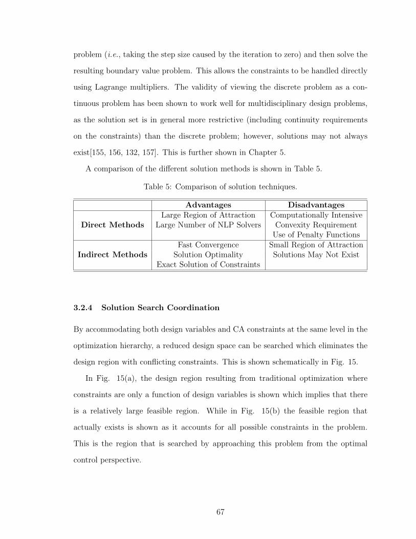
problem (i.e., taking the step size caused by the iteration to zero) and then solve the
resulting boundary value problem. This allows the constraints to be handled directly
using Lagrange multipliers. The validity of viewing the discrete problem as a con-
tinuous problem has been shown to work well for multidisciplinary design problems,
as the solution set is in general more restrictive (including continuity requirements
on the constraints) than the discrete problem; however, solutions may not always
exist[155, 156, 132, 157]. This is further shown in Chapter 5.
A comparison of the different solution methods is shown in Table 5.
Table 5: Comparison of solution techniques.
Advantages Disadvantages
Direct MethodsLarge Region of Attraction Computationally Intensive
Large Number of NLP Solvers Convexity RequirementUse of Penalty Functions
Indirect MethodsFast Convergence Small Region of Attraction
Solution Optimality Solutions May Not ExistExact Solution of Constraints
3.2.4 Solution Search Coordination
By accommodating both design variables and CA constraints at the same level in the
optimization hierarchy, a reduced design space can be searched which eliminates the
design region with conflicting constraints. This is shown schematically in Fig. 15.
In Fig. 15(a), the design region resulting from traditional optimization where
constraints are only a function of design variables is shown which implies that there
is a relatively large feasible region. While in Fig. 15(b) the feasible region that
actually exists is shown as it accounts for all possible constraints in the problem.
This is the region that is searched by approaching this problem from the optimal
control perspective.
67
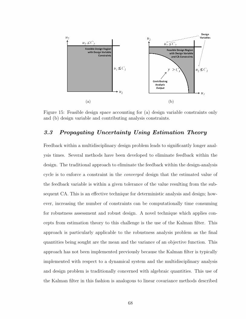
(a)
y
(b)
Figure 15: Feasible design space accounting for (a) design variable constraints onlyand (b) design variable and contributing analysis constraints.
3.3 Propagating Uncertainty Using Estimation Theory
Feedback within a multidisciplinary design problem leads to significantly longer anal-
ysis times. Several methods have been developed to eliminate feedback within the
design. The traditional approach to eliminate the feedback within the design-analysis
cycle is to enforce a constraint in the converged design that the estimated value of
the feedback variable is within a given tolerance of the value resulting from the sub-
sequent CA. This is an effective technique for deterministic analysis and design; how-
ever, increasing the number of constraints can be computationally time consuming
for robustness assessment and robust design. A novel technique which applies con-
cepts from estimation theory to this challenge is the use of the Kalman filter. This
approach is particularly applicable to the robustness analysis problem as the final
quantities being sought are the mean and the variance of an objective function. This
approach has not been implemented previously because the Kalman filter is typically
implemented with respect to a dynamical system and the multidisciplinary analysis
and design problem is traditionally concerned with algebraic quantities. This use of
the Kalman filter in this fashion is analogous to linear covariance methods described
68
in Refs. [82, 83, 84] and Appendix A.
3.3.1 The Discrete Kalman Filter
The Kalman filter can be thought of as a two step process, one which predicts the
state (e.g., the output of the CAs) and then an update step which corrects these
estimates based on the dynamics of the system. The prediction step is given by the
following equations[82, 135, 158, 159, 160, 161, 162]
yk|k−1 = Fkyk−1|k−1 + Bkuk (62)
Σk|k−1 = FkΣk−1|k−1FTk + Qk (63)
where the notation j|k represents the estimate at j given observations up to and
including k. Furthermore, the value of y0|0 is the initial mean state and Σ0|0 is the
initial covariance matrix of the state values. The correction step is governed by the
following equations[82, 135, 158, 159, 160, 161, 162]
xk = zk −Hkyk|k−1 (64)
Sk = HkΣk|k−1HTk + Rk (65)
Kk = Σk|k−1HTkS−1
k (66)
yk|k = yk|k−1 + Kkxk (67)
Σk|k = (I−KkHk) Σk|k−1 (68)
where the final (a posteriori) estimate of the state is given by yk|k with covariance
matrix given by Σk|k.
3.3.2 Formulating the Multidisciplinary Design Problem in a Form Com-patible with the Kalman Filter
The root-finding problem has been shown to be a dynamical system which can be
defined by the relation
yk = f(yk−1), ∀k ∈ Z+ \ 0 (69)
69
where f(yk−1) is the output value of the CAs on the kth − 1 iteration. For random
variables in a linear system, this can be written in the form
yk = Fkyk−1 + wk−1, ∀k ∈ Z+ \ 0 (70)
where wk−1 is the noise associated with the model. For a linear multidisciplinary
design, Eq. (70) can also be written as
yk = Fkyk−1 + Bkuk + wk−1 (71)
which allows for inputs into the CA that are not outputs of other CAs, uk. When
coupled with an equation of the form
zk = Hkyk + vk (72)
and when it is assumed that wk−1 ∼ N (0,Qk−1) and vk−1 ∼ N (0,Rk−1), Eqs. (71)
and (72) define the dynamical system needed for a Kalman filter[158, 159, 160, 161].
The noise parameter, wk−1, gives the opportunity to account for random variables
within the linearization of the input-output relationship, that is random variables
associated with the matrix F. In this work, the Kalman filter is used as a data fusion
technique to give an optimal unbiased statistical estimate of the output of the CAs
as the design is converging.
The power in implementing the Kalman filter in multidisciplinary design analysis
lies in the ability to obtain a continuous estimate in iterate of both the mean and co-
variance of each CA’s output in the multidisciplinary design by propagating a system
of seven equations until the design converges.
3.3.3 Using the Covariance Matrix to Guide Design Decomposition
As one of the outputs of the Kalman filter is the estimated covariance at iteration k
this information could be used to ascertain the correlation coefficient between vari-
ables. Provided the covariance estimate, Σ, has the form of Eq. (12) and can be
70
represented as
Σ = Σij (73)
then the representative correlation (or product-moment) coefficients are given by
ρij =Σij√
Σii
√Σjj
, i 6= j (74)
where ρij ∈ [−1, 1]. What is important about the correlation coefficient is that it
gives a relative measure of how variable j depends on variable i. In particular as
|ρij| → 1 the importance of variable i on the response of variable j increases. This
gives a meaningful way to ascertain the importance of each CA and variables on other
CAs and variables. For design decomposition, it may be acceptable to neglect the
feedback variables with small correlation coefficient magnitudes.
3.4 Summary
This chapter provides the theory behind application of three techniques from dynam-
ical system theory to the multidisciplinary design problem. Stability analysis was
shown to be useful in determining whether a design is feasible, whether an optimal
design exists, the range of initial values that can be used to converge the design, and
the rate at which the design will converge. Control theory is shown to be capable of
enforcing constraints that are functions of the CA’s output and the design variables
at the same level in the optimization hierarchy. Finally, estimation theory is shown
to be capable of propagating uncertainty through the multidisciplinary design, pro-
viding a method to simultaneously converge the design and quantify the uncertainty
associated with each design point.
71
CHAPTER IV
DEVELOPMENT OF A FRAMEWORK FOR THE RAPID
ROBUST DESIGN OF MULTIDISCIPLINARY SYSTEMS
This chapter takes the foundations set forth in Chapter 2 to view the multidisciplinary
design problem as a dynamical system to develop a comprehensive rapid robust design
framework for linear designs that utilizes dynamical system theory. This methodology
uses the three techniques described in Chapter 3, stability analysis, control theory, and
estimation theory as an ensemble. A framework is developed for two different root-
finding techniques—fixed-point iteration and Newton-Raphson iteration, although it
is extensible to other numerical root-finding methods that are recursive. A discussion
is also provided about how to extend this inherently linearly framework to nonlinear
multidisciplinary design through successive linearization.
4.1 A Rapid Design Robustness Analysis Framework
The cumulative contribution of this work is the ability to rapidly obtain a bound on
the robustness of a multidisciplinary system by posing the multidisciplinary design
problem as a dynamical system. In particular, a methodology that rapidly obtains
the mean and a bound on the variance of a multidisciplinary design’s response is
developed. The theoretical development of this methodology is restricted to linear
multidisciplinary designs. This implies a CA whose output, y, can be functionally
represented as a linear combination of the inputs into the CA, x, and an offset, b, or
y = Ax + b. While this may seem to be a restrictive framework in which to operate,
as in many engineering analyses, linearization can be employed to allow the CAs to fit
this functional form. With the mean and variance bound found, traditional measures
72
of design robustness can be obtained (e.g., the mean, variance, MSD, etc.). Many
robustness assessment techniques, particularly those associated with NLP solutions,
require solution of a large number of trials. These trials consist of input variables
being drawn from distributions and then converging the design through iteration
in order to obtain the performance for that trial. The robustness of the design is
then ascertained by repeating this process until the output distribution is formed.
The methodology developed in this work circumvents the time intensive process of
propagating individual trials to obtain the output distribution by using the mean and
covariance matrix (the typical quantities needed to define robustness) directly and
then derives a bound on the response’s variance. With such a technique in place to
obtain estimates on the mean and variance, the design robustness may be directly
traded early in the design process.
A general multidisciplinary design features coupling between CAs. This may lead
to convergence issues, potentially requiring significant iteration in order to converge
on a design. As discussed previously, the iteration scheme implemented to find the
solution to the multidisciplinary design can be cast as a dynamical system where the
state is the output of each of the CAs and the fixed rule describing its evolution is
the method used to find the root of the design. In order to examine the existence of
a solution, the first application of this new perspective of multidisciplinary design is
used—stability analysis. If the dynamical system described by an iteration scheme
is asymptotically stable, there exists at least some solution to the multidisciplinary
design.
Another enabling technique for this methodology is in the handling of the multidis-
ciplinary design requirements. These are generally written as equality and inequality
constraints that are functions of the state. The iteration scheme implicitly handles
the compatibility constraints within the multidisciplinary design, a general statement
that each CA in a converged design must use the same information. Other constraints
73
must be handled by more explicit techniques. By viewing the multidisciplinary de-
sign as a dynamical system, design constraints are able to be handled through similar
techniques as state and control constraints in optimal control, where the constraints
are added to the objective function. Adjoining these constraints allows the design
variables to appear explicitly in the objective function formulation. This method
allows for simultaneous handling of constraints of the outputs of each CA, which are
the coupling variables in the design, as well as the design variables.
The last of the the dynamical system techniques employed in this work to obtain
a rapid assessment of the design robustness is the use of an estimation technique
traditionally applied to state estimation, the Kalman filter. The Kalman filter is a
statistical estimation technique for linear dynamical systems which combines mea-
surements to estimate the true dynamics of the system. The multidisciplinary design
utilization of the Kalman filter allows for the mean (or nominal) and the covariance
matrix of each CA’s output to be found simultaneously as a function of iterate num-
ber. In this sense, the propagation of the filter equations can be used to converge the
design and provide estimates of robustness instead of requiring convergence for each
Monte Carlo sample, as in traditional robustness analysis.
Two additional techniques from non-traditional design fields are also used in the
methodology. The first of these is the unscented transform, which is a statistical
transformation that gives accurate estimates of the first two moments of the output
probability distribution of a CA while only evaluating a small sample of carefully
chosen points, the sigma points. This technique, is similar to a Monte Carlo; how-
ever, third order accuracy of the mean and covariance matrix is maintained for any
functional form of the CA despite the small number of trials (sigma points) evalu-
ated. The last enabling technique used in this work is the two-norm of a matrix. The
matrix two-norm provides a conservative bound for the output covariance variance,
as it finds the principal eigenvalue (i.e., the “variance” along the principal direction
74
of the covariance matrix). This quantity gives a bound on the variance and, as shown
later, can be used as a direct surrogate for the variance for fixed distributions as the
observed error remains identical.
4.2 A Rapid Robust Design Methodology
The following section describes a rapid robust design methodology that implements
a matrix-norm to obtain a bound on the variance of a multidisciplinary system which
can be decomposed into CAs.
4.2.1 Formulation with Fixed-Point Iteration
Step 1: Decompose the Design
A general multidisciplinary design can be decomposed into multiple CAs. Each of
these CAs represents an analysis that contributes to the entire design. For example,
consider the design or analysis of an entry system. It may be desired for the entry
system to be evaluated with respect to its payload capability and landing accuracy.
Many different analyses must be conducted in order to obtain this information. This
information flow is shown in Fig. 16, where one such representation of each of the
analyses that must be conducted to design an entry system is shown[163]. In this
case, the entry system is decomposed into seven CAs. The responses of these CAs
allow the payload capability as well as the landed accuracy to be assessed. Each CA
in Fig. 16 (i.e., the blocks) represents an input-output relationship. For instance,
inputs into the aerodynamics analysis include the configuration of the entry system
and planetary body where it is to operate; outputs include the force coefficients of the
vehicle as a function of Mach number and attitude. This relationship may be known
analytically; however, it is more likely that this CA would represent a computational
analysis that is linked into the design process. This decomposition is also analogous
to that required by other MDO techniques, such as SSA, OBD, and CO and therefore
requires no additional upfront computational time.
75

System Definition
Planetary Model
Guidance, Navigation, and
Control
Trajectory Analysis
Thermal Response
Weights and Sizing
System Aerodynamics
Figure 16: The decomposition of an entry system into a Design Structure Matrix.
In the theoretical development underlying this work, it is assumed that each of
the n CAs are linear and algebraic. This limitation will be addressed subsequently.
That is, the output of the CA is of the form
yj = Ajy + Bjud + Cjup + dj (75)
where yj ∈ Rlj , y ∈ Rm is the concatenated output from all of the CAs (e.g., if
y1, y2 through yn are the outputs of the n CAs in a multidisciplinary design, y =(y1
T y2T · · · yn
T)T
), ud ∈ Rd are the deterministic system-level inputs into the
design, up ∈ Rp are the probabilistic system-level inputs into the design, and dj ∈
Rlj is the bias associated with the model. This implies Aj ∈ Rlj×m, Bj ∈ Rlj×d,
Cj ∈ Rlj×p, and thatn∑j=1
lj = m.
For general designs where the CAs may not be linear, the required functional form
can be achieved through linearization where Aj =∂g
∂y
∣∣∣y, Bj =
∂g
∂ud
∣∣∣ud
, Cj =∂g
∂up
∣∣∣up
,
and
dj = − (Ajy + Bjud + Cjup)
when the input-output relationship for the CA is given by yj = g (y,ud,up) and (·)
76
is the value of (·) about which the function is linearized. During the iteration, (·) is
the value of (·) from the prior iteration.
Step 2: Identify the Random Variables and their Distributions
In the design and analysis of a complex multidisciplinary system, it is unlikely that
each of the models and inputs are deterministic; instead, many are likely to be proba-
bilistic and account for unknowns in the modeling and in the operating conditions . In
order to propagate these uncertainties through the design to estimate the robustness,
the probabilistic variables must be identified.
The random variables associated with the uncertainty within the design are han-
dled in two different ways in this work depending on where the random variable is
functionally located. Functionally, the uncertainty resulting from inputs into the CA
refers to uncertainties associated with up, whereas uncertainty associated with the
physical modeling pertain to Aj, Bj, Cj, or dj. In the first instance, the mean is
propagated in the yk|k term of the filter equations and the covariance is propagated
in the Σk|k term of the filter equations. In the second case, the mean is again ac-
counted for in the yk|k term of the equations; however, the covariance is accounted
for in the Qk term of the filter. In the components of the Kalman filter mentioned,
the notation k|k refers to the kth iteration of the filter given all previous information
regarding the convergence of the system.
Due to the the propagation within the Kalman filter there is an assumption that
the uncertainties associated with the model are Gaussian. For symmetrical proba-
bility distributions (i.e., probability distributions centered about the mean), this is
not an overly strong assumption since the first two moments are the only terms be-
ing approximated. However, for asymmetric probability distributions, this becomes
a restrictive assumption that is a limitation of this technique.
77
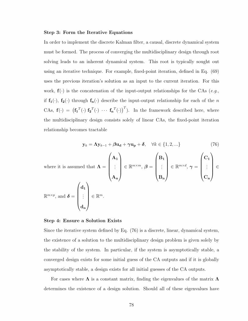
Step 3: Form the Iterative Equations
In order to implement the discrete Kalman filter, a causal, discrete dynamical system
must be formed. The process of converging the multidisciplinary design through root
solving leads to an inherent dynamical system. This root is typically sought out
using an iterative technique. For example, fixed-point iteration, defined in Eq. (69)
uses the previous iteration’s solution as an input to the current iteration. For this
work, f(·) is the concatenation of the input-output relationships for the CAs (e.g.,
if f1(·), f2(·) through fn(·) describe the input-output relationship for each of the n
CAs, f(·) =(f1T (·) f2
T (·) · · · fnT (·)
)T). In the framework described here, where
the multidisciplinary design consists solely of linear CAs, the fixed-point iteration
relationship becomes tractable
yk = Λyk−1 + βud + γup + δ, ∀k ∈ 1, 2, ... (76)
where it is assumed that Λ =
A1
...
An
∈ Rm×m, β =
B1
...
Bn
∈ Rm×d, γ =
C1
...
Cn
∈
Rm×p, and δ =
d1
...
dn
∈ Rm.
Step 4: Ensure a Solution Exists
Since the iterative system defined by Eq. (76) is a discrete, linear, dynamical system,
the existence of a solution to the multidisciplinary design problem is given solely by
the stability of the system. In particular, if the system is asymptotically stable, a
converged design exists for some initial guess of the CA outputs and if it is globally
asymptotically stable, a design exists for all initial guesses of the CA outputs.
For cases where Λ is a constant matrix, finding the eigenvalues of the matrix Λ
determines the existence of a design solution. Should all of these eigenvalues have
78
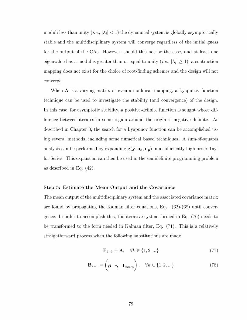
moduli less than unity (i.e., |λi| < 1) the dynamical system is globally asymptotically
stable and the multidisciplinary system will converge regardless of the initial guess
for the output of the CAs. However, should this not be the case, and at least one
eigenvalue has a modulus greater than or equal to unity (i.e., |λi| ≥ 1), a contraction
mapping does not exist for the choice of root-finding schemes and the design will not
converge.
When Λ is a varying matrix or even a nonlinear mapping, a Lyapunov function
technique can be used to investigate the stability (and convergence) of the design.
In this case, for asymptotic stability, a positive-definite function is sought whose dif-
ference between iterates in some region around the origin is negative definite. As
described in Chapter 3, the search for a Lyapunov function can be accomplished us-
ing several methods, including some numerical based techniques. A sum-of-squares
analysis can be performed by expanding g(y,ud,up) in a sufficiently high-order Tay-
lor Series. This expansion can then be used in the semidefinite programming problem
as described in Eq. (42).
Step 5: Estimate the Mean Output and the Covariance
The mean output of the multidisciplinary system and the associated covariance matrix
are found by propagating the Kalman filter equations, Eqs. (62)-(68) until conver-
gence. In order to accomplish this, the iterative system formed in Eq. (76) needs to
be transformed to the form needed in Kalman filter, Eq. (71). This is a relatively
straightforward process when the following substitutions are made
Fk−1 = Λ, ∀k ∈ 1, 2, ... (77)
Bk−1 =
(β γ Im×m
), ∀k ∈ 1, 2, ... (78)
79
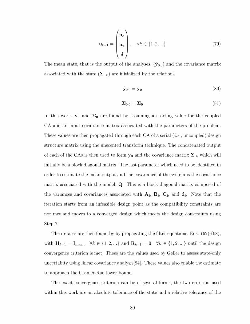
uk−1 =
ud
up
δ
, ∀k ∈ 1, 2, ... (79)
The mean state, that is the output of the analyses, (y0|0) and the covariance matrix
associated with the state (Σ0|0) are initialized by the relations
y0|0 = y0 (80)
Σ0|0 = Σ0 (81)
In this work, y0 and Σ0 are found by assuming a starting value for the coupled
CA and an input covariance matrix associated with the parameters of the problem.
These values are then propagated through each CA of a serial (i.e., uncoupled) design
structure matrix using the unscented transform technique. The concatenated output
of each of the CAs is then used to form y0 and the covariance matrix Σ0, which will
initially be a block diagonal matrix. The last parameter which need to be identified in
order to estimate the mean output and the covariance of the system is the covariance
matrix associated with the model, Q. This is a block diagonal matrix composed of
the variances and covariances associated with Aj, Bj, Cj, and dj. Note that the
iteration starts from an infeasible design point as the compatibility constraints are
not met and moves to a converged design which meets the design constraints using
Step 7.
The iterates are then found by by propagating the filter equations, Eqs. (62)-(68),
with Hk−1 = Im×m ∀k ∈ 1, 2, ... and Rk−1 = 0 ∀k ∈ 1, 2, ... until the design
convergence criterion is met. These are the values used by Geller to assess state-only
uncertainty using linear covariance analysis[84]. These values also enable the estimate
to approach the Cramer-Rao lower bound.
The exact convergence criterion can be of several forms, the two criterion used
within this work are an absolute tolerance of the state and a relative tolerance of the
80

state. These are demonstrated in the following relations
‖ yk|k − yk−1|k−1 ‖2≤ ε1 (82)
‖ yk|k − yk−1|k−1 ‖2
‖ yk−1|k−1 ‖2
≤ ε2 (83)
Step 6: Identify the Mean and Variance Bound of the Objective Function
Assume the design objective is a linear combination of the outputs of linear CAs,
that is
r = My∗ (84)
where r ∈ R is the design objective value, M ∈ R1×q is a matrix describing the linear
combination of the pertinent CA outputs, and y∗ ∈ Rq is the vector of pertinent
CA responses that contribute to the design objective. An estimate of the mean and
variance bound for the design objective can be found as follows
r = My∗n|n (85)
σ2r ≤‖ Σy∗n|n ‖2 M1q (86)
where it is assumed the n iterations have occurred and Σy∗n|n is the reduced covari-
ance matrix associated with only the variables associated with y∗ (i.e., the rows and
columns of the variables not pertinent in the design objective are eliminated from
Σyn|n). Additionally, the notation 1q ∈ Rq×1 is the unity vector of length q (i.e.,
1q = (1 1 1 · · · 1)T ∈ Rq×1).
More generally, a first-order expansion of an objective function that is of the form
r = g(y∗) (87)
can be made. The linearized objective function, Eq. (87), about y∗nom is then given
by
r =∂g
∂y∗y∗ − ∂g
∂y∗y∗nom = Ny∗ + b (88)
81
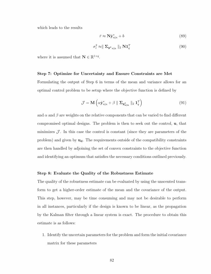
which leads to the results
r ≈ Ny∗n|n + b (89)
σ2r ≈‖ Σy∗n|n ‖2 N1Tq (90)
where it is assumed that N ∈ R1×q.
Step 7: Optimize for Uncertainty and Ensure Constraints are Met
Formulating the output of Step 6 in terms of the mean and variance allows for an
optimal control problem to be setup where the objective function is defined by
J = M(αy∗n|n + β ‖ Σy∗
n|n‖2 1Tq
)(91)
and α and β are weights on the relative components that can be varied to find different
compromised optimal designs. The problem is then to seek out the control, u, that
minimizes J . In this case the control is constant (since they are parameters of the
problem) and given by ud. The requirements outside of the compatibility constraints
are then handled by adjoining the set of convex constraints to the objective function
and identifying an optimum that satisfies the necessary conditions outlined previously.
Step 8: Evaluate the Quality of the Robustness Estimate
The quality of the robustness estimate can be evaluated by using the unscented trans-
form to get a higher-order estimate of the mean and the covariance of the output.
This step, however, may be time consuming and may not be desirable to perform
in all instances, particularly if the design is known to be linear, as the propagation
by the Kalman filter through a linear system is exact. The procedure to obtain this
estimate is as follows:
1. Identify the uncertain parameters for the problem and form the initial covariance
matrix for these parameters
82
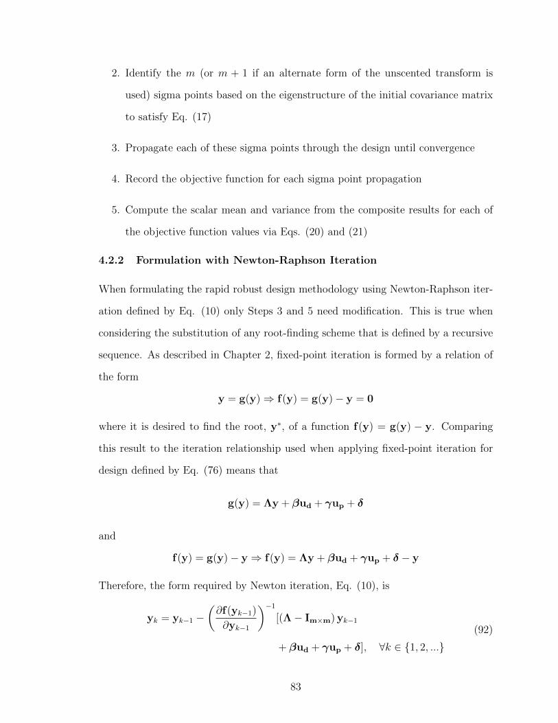
2. Identify the m (or m + 1 if an alternate form of the unscented transform is
used) sigma points based on the eigenstructure of the initial covariance matrix
to satisfy Eq. (17)
3. Propagate each of these sigma points through the design until convergence
4. Record the objective function for each sigma point propagation
5. Compute the scalar mean and variance from the composite results for each of
the objective function values via Eqs. (20) and (21)
4.2.2 Formulation with Newton-Raphson Iteration
When formulating the rapid robust design methodology using Newton-Raphson iter-
ation defined by Eq. (10) only Steps 3 and 5 need modification. This is true when
considering the substitution of any root-finding scheme that is defined by a recursive
sequence. As described in Chapter 2, fixed-point iteration is formed by a relation of
the form
y = g(y)⇒ f(y) = g(y)− y = 0
where it is desired to find the root, y∗, of a function f(y) = g(y) − y. Comparing
this result to the iteration relationship used when applying fixed-point iteration for
design defined by Eq. (76) means that
g(y) = Λy + βud + γup + δ
and
f(y) = g(y)− y⇒ f(y) = Λy + βud + γup + δ − y
Therefore, the form required by Newton iteration, Eq. (10), is
yk = yk−1 −(∂f(yk−1)
∂yk−1
)−1
[(Λ− Im×m) yk−1
+ βud + γup + δ], ∀k ∈ 1, 2, ...(92)
83
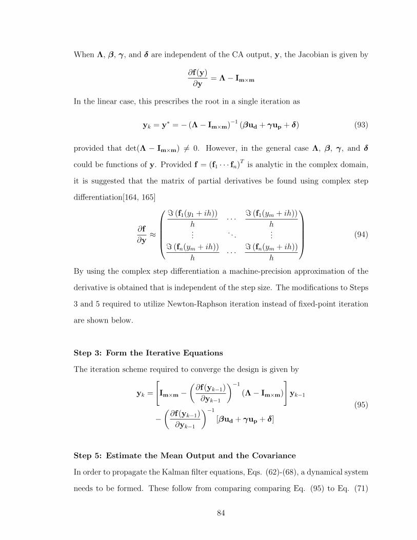
When Λ, β, γ, and δ are independent of the CA output, y, the Jacobian is given by
∂f(y)
∂y= Λ− Im×m
In the linear case, this prescribes the root in a single iteration as
yk = y∗ = − (Λ− Im×m)−1 (βud + γup + δ) (93)
provided that det(Λ − Im×m) 6= 0. However, in the general case Λ, β, γ, and δ
could be functions of y. Provided f = (f1 · · · fn)T is analytic in the complex domain,
it is suggested that the matrix of partial derivatives be found using complex step
differentiation[164, 165]
∂f
∂y≈
= (f1(y1 + ih))
h· · · = (f1(ym + ih))
h...
. . ....
= (fn(ym + ih))
h· · · = (fn(ym + ih))
h
(94)
By using the complex step differentiation a machine-precision approximation of the
derivative is obtained that is independent of the step size. The modifications to Steps
3 and 5 required to utilize Newton-Raphson iteration instead of fixed-point iteration
are shown below.
Step 3: Form the Iterative Equations
The iteration scheme required to converge the design is given by
yk =
[Im×m −
(∂f(yk−1)
∂yk−1
)−1
(Λ− Im×m)
]yk−1
−(∂f(yk−1)
∂yk−1
)−1
[βud + γup + δ]
(95)
Step 5: Estimate the Mean Output and the Covariance
In order to propagate the Kalman filter equations, Eqs. (62)-(68), a dynamical system
needs to be formed. These follow from comparing comparing Eq. (95) to Eq. (71)
84
as was done in the case of fixed-point iteration. The following results after this
comparison
Fk−1 = Im×m −(∂f(yk−1)
∂yk−1
)−1
(Λ− Im×m) , ∀k ∈ 1, 2, ... (96)
Bk−1 =
βT(∂f(yk−1)
∂yk−1
)−TγT(∂f(yk−1)
∂yk−1
)−T(∂f(yk−1)
∂yk−1
)−T
T
, ∀k ∈ 1, 2, ... (97)
uk−1 =
ud
up
δ
, ∀k ∈ 1, 2, ... (98)
4.3 Summary
This chapter took the techniques described in Chapter 3 to develop an eight step
methodology to rapidly obtain a robust design. The steps of this methodology are
shown below
1. Decompose the design
2. Identify the random variables in the design and their distributions
3. Form the iterative equations
4. Ensure a solution exists
5. Estimate the mean output and the covariance of the design
6. Identify the mean and variance bound of the objective function
7. Optimize for uncertainty and ensure constraints are met
8. Evaluate the quality of the robustness estimate for nonlinear designs
85

While the theoretical development is restricted to linear systems due to the Kalman
filter being utilized, extensions via successive linearization to nonlinear designs were
discussed. The flexibility of the methodology to accommodate different numerical
root-finding algorithms was also demonstrated through formulation of an alternate
methodology with Newton iteration. Note that there is no additional upfront com-
putational time compared to other MDO techniques.
86

CHAPTER V
DEMONSTRATION OF DYNAMICAL SYSTEM THEORY
APPLIED TO THE MULTIDISCIPLINARY DESIGN
PROBLEM
This chapter demonstrates the dynamical system techniques developed to illustrative
multidisciplinary design problems. This begins with an analytical, linear example that
describes the accuracy of the estimation technique to propagate uncertainty within
the design as well as a quantization of its performance relative to industry-standard
techniques. Then the methods to find the region of initial guesses required to converge
the design (i.e., make the design asymptotically stable) and examine the rate of
convergence are demonstrated. Then three robust design applications are presented.
One linear, analytical example and two nonlinear applications. The last application
shows the application of the developed methodology to a practical problem relevant
to the entry, descent, and landing community, the design of a deployable device to
increase the range or accuracy of an existing strategic system. For each of these
design applications comparison is made to traditional techniques.
5.1 Accuracy of the Mean and Variance Estimate
To show the accuracy of the mean and variance estimate provided by the rapid robust
design methodology, consider the coupled, linear two CA system shown in Fig. 17.
For this analysis, assume that there are two components to the probabilistic parameter
vector and the two output vectors, that is up ∈ R2, y1 ∈ R2, and y2 ∈ R2, which,
in turn, implies A′1 ∈ R2×2, B′1 ∈ R2, C′1 ∈ R2×2, A′2 ∈ R2×2, and B′2 ∈ R2. Also,
let the distribution of the probabilistic parameter input be given by a multivariate
87
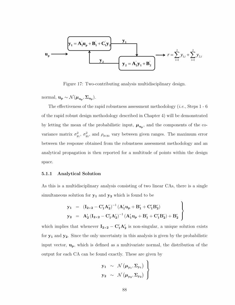
2
'
1
'
1p
'
11 yCBuAy
'
21
'
22 ByAy
2
1
,2
2
1
,1
i
i
i
i yyrpu
1y
2y
Figure 17: Two-contributing analysis multidisciplinary design.
normal, up ∼ N (µup,Σup).
The effectiveness of the rapid robustness assessment methodology (i.e., Steps 1 - 6
of the rapid robust design methodology described in Chapter 4) will be demonstrated
by letting the mean of the probabilistic input, µup, and the components of the co-
variance matrix σ2y1
, σ2y2
, and ρy1y2 vary between given ranges. The maximum error
between the response obtained from the robustness assessment methodology and an
analytical propagation is then reported for a multitude of points within the design
space.
5.1.1 Analytical Solution
As this is a multidisciplinary analysis consisting of two linear CAs, there is a single
simultaneous solution for y1 and y2 which is found to be
y1 = (I2×2 −C′1A′2)−1 (A′1up + B′1 + C′1B′2)
y2 = A′2 (I2×2 −C′1A′2)−1 (A′1up + B′1 + C′1B′2) + B′2
which implies that whenever I2×2 − C′1A′2 is non-singular, a unique solution exists
for y1 and y2. Since the only uncertainty in this analysis is given by the probabilistic
input vector, up, which is defined as a multivariate normal, the distribution of the
output for each CA can be found exactly. These are given by
y1 ∼ N(µy1
,Σy1
)y2 ∼ N
(µy2
,Σy2
)
88
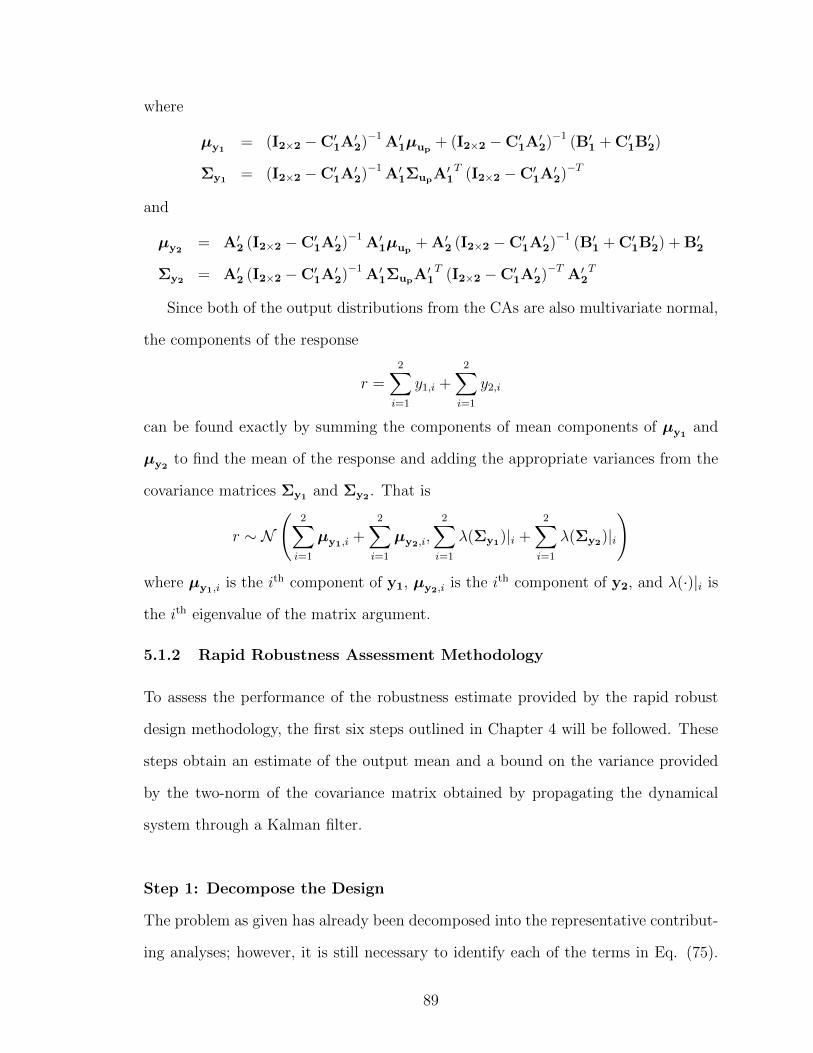
where
µy1= (I2×2 −C′1A′2)−1 A′1µup
+ (I2×2 −C′1A′2)−1 (B′1 + C′1B′2)
Σy1 = (I2×2 −C′1A′2)−1 A′1ΣupA′1T (I2×2 −C′1A′2)−T
and
µy2= A′2 (I2×2 −C′1A′2)−1 A′1µup
+ A′2 (I2×2 −C′1A′2)−1 (B′1 + C′1B′2) + B′2
Σy2 = A′2 (I2×2 −C′1A′2)−1 A′1ΣupA′1T (I2×2 −C′1A′2)−T A′2
T
Since both of the output distributions from the CAs are also multivariate normal,
the components of the response
r =2∑i=1
y1,i +2∑i=1
y2,i
can be found exactly by summing the components of mean components of µy1and
µy2to find the mean of the response and adding the appropriate variances from the
covariance matrices Σy1 and Σy2 . That is
r ∼ N
(2∑i=1
µy1,i +2∑i=1
µy2,i,2∑i=1
λ(Σy1)|i +2∑i=1
λ(Σy2)|i
)where µy1,i is the ith component of y1, µy2,i is the ith component of y2, and λ(·)|i is
the ith eigenvalue of the matrix argument.
5.1.2 Rapid Robustness Assessment Methodology
To assess the performance of the robustness estimate provided by the rapid robust
design methodology, the first six steps outlined in Chapter 4 will be followed. These
steps obtain an estimate of the output mean and a bound on the variance provided
by the two-norm of the covariance matrix obtained by propagating the dynamical
system through a Kalman filter.
Step 1: Decompose the Design
The problem as given has already been decomposed into the representative contribut-
ing analyses; however, it is still necessary to identify each of the terms in Eq. (75).
89
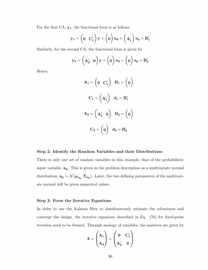
For the first CA, y1, the functional form is as follows
y1 =
(0 C′1
)y +
(0
)ud +
(A′1
)up + B′1
Similarly, for the second CA, the functional form is given by
y2 =
(A′2 0
)y +
(0
)ud +
(0
)up + B′2
Hence,
A1 =
(0 C′1
)B1 =
(0
)
C1 =
(A′1
)d1 = B′1
A2 =
(A′2 0
)B2 =
(0
)
C2 =
(0
)d2 = B′2
Step 2: Identify the Random Variables and their Distributions
There is only one set of random variables in this example, that of the probabilistic
input variable, up. This is given in the problem description as a multivariate normal
distribution, up ∼ N (µup,Σup). Later, the two defining parameters of the multivari-
ate normal will be given numerical values.
Step 3: Form the Iterative Equations
In order to use the Kalman filter to simultaneously estimate the robustness and
converge the design, the iterative equations described in Eq. (76) for fixed-point
iteration need to be formed. Through analogy of variables, the matrices are given by
Λ =
A1
A2
=
0 C′1
A′2 0
90
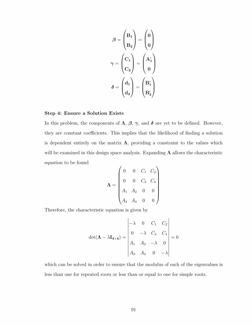
β =
B1
B2
=
0
0
γ =
C1
C2
=
A′1
0
δ =
d1
d2
=
B′1
B′2
Step 4: Ensure a Solution Exists
In this problem, the components of Λ, β, γ, and δ are yet to be defined. However,
they are constant coefficients. This implies that the likelihood of finding a solution
is dependent entirely on the matrix Λ, providing a constraint to the values which
will be examined in this design space analysis. Expanding Λ allows the characteristic
equation to be found
Λ =
0 0 C1 C2
0 0 C3 C4
A1 A2 0 0
A3 A4 0 0
Therefore, the characteristic equation is given by
det(Λ− λI4×4) =
∣∣∣∣∣∣∣∣∣∣∣∣∣
−λ 0 C1 C2
0 −λ C3 C4
A1 A2 −λ 0
A3 A4 0 −λ
∣∣∣∣∣∣∣∣∣∣∣∣∣= 0
which can be solved in order to ensure that the modulus of each of the eigenvalues is
less than one for repeated roots or less than or equal to one for simple roots.
91
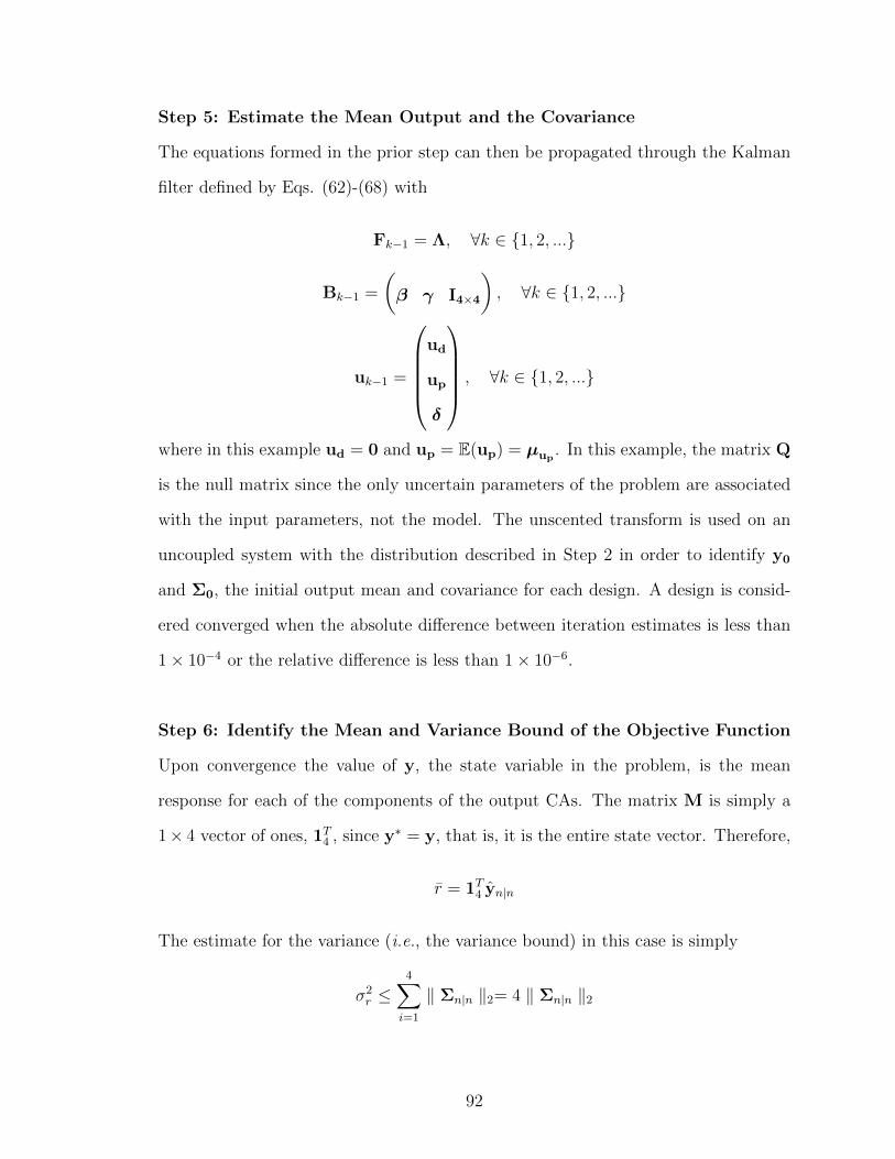
Step 5: Estimate the Mean Output and the Covariance
The equations formed in the prior step can then be propagated through the Kalman
filter defined by Eqs. (62)-(68) with
Fk−1 = Λ, ∀k ∈ 1, 2, ...
Bk−1 =
(β γ I4×4
), ∀k ∈ 1, 2, ...
uk−1 =
ud
up
δ
, ∀k ∈ 1, 2, ...
where in this example ud = 0 and up = E(up) = µup. In this example, the matrix Q
is the null matrix since the only uncertain parameters of the problem are associated
with the input parameters, not the model. The unscented transform is used on an
uncoupled system with the distribution described in Step 2 in order to identify y0
and Σ0, the initial output mean and covariance for each design. A design is consid-
ered converged when the absolute difference between iteration estimates is less than
1× 10⁻⁴ or the relative difference is less than 1× 10⁻⁶.
Step 6: Identify the Mean and Variance Bound of the Objective Function
Upon convergence the value of y, the state variable in the problem, is the mean
response for each of the components of the output CAs. The matrix M is simply a
1× 4 vector of ones, 1T4 , since y∗ = y, that is, it is the entire state vector. Therefore,
r = 1T4 yn|n
The estimate for the variance (i.e., the variance bound) in this case is simply
σ2r ≤
4∑i=1
‖ Σn|n ‖2= 4 ‖ Σn|n ‖2
92
5.1.3 Analysis Results
In order to assess a large variety of problems, a parametric sweep of the design
variables was performed to identify the maximum errors in the design space. To
perform this parameter sweep, the problem’s parameters were varied independently
as shown in Table 6 where the distribution of each variable was assumed to be uniform
and a 100,000 case Monte Carlo analysis was conducted.
Table 6: Parameter ranges to assess the validity of the rapid robust design method-ology.
Parameter Distributionσ2
1 U(0, 100)σ2
2 U(0, 100)ρy1y2 U(−1, 1)
A′1
(U(−1, 1) U(−1, 1)U(−1, 1) U(−1, 1)
)B′1
(U(−1, 1)U(−1, 1)
)C′1
(U(−1, 1) U(−1, 1)U(−1, 1) U(−1, 1)
)A′2
(U(−1, 1) U(−1, 1)U(−1, 1) U(−1, 1)
)B′2
(U(−1, 1)U(−1, 1)
)
In order to guarantee convergence of the design, constraints were imposed on the
parameters to ensure that all of the eigenvalues of the matrix Λ had modulus less than
unity. To ensure realizable covariance matrices, that is a matrix that is symmetric
and positive definite, the components of the covariance (e.g., variance and correlation
coefficient) were determined independently and then combined to form the covariance
matrix.
In addition to the parameters shown in Table 6, the effect of the mean of the
probabilistic parameters was conducted by analyzing three different cases–one where
the mean was µup= (0 0)T , one where the mean was µup
= (100 0)T , and one
93
where the mean was µup= (100 100)T . The results were then compared with results
propagated analytically resulting in Figs. 18-20.
It is observed from these results that the mean error is less than 0.08% for all
of the cases examined. This is a result of the system being linear and the Kalman
filter propagating results exactly for a linear system. Therefore the error in the mean
is solely a result of the convergence criterion being utilized. For each case, there is
seen to be a rise in the standard deviation error near the origin. This is because the
nominal mean goes to zero causing a rise in the in the percent error near this point.
The rapid robustness assessment methodology is observed to provide a consistent
conservative bound on the variance as seen in Figs. 18-20 since all of the percent
error values are positive. It is also interesting to note that the error in mean and
standard deviation, regardless of the mean of the input, appears to be close to the
same order of magnitude. As the mean input value increases, the magnitude of the
mean response and standard deviation of that response increases, which causes a
decrease in the percent error. Furthermore, it is observed that the maximum error
approaches a limit of less than 40%. This limit is a function of the two-norm being
used. This limit is described and related to the dimensionality of the problem in
Chapter 6. In analyzing the data, the largest errors are caused for weakly coupled
systems, that is systems where C′1 is small. This can be explained since C′1 being
small leads to a larger domain of values that lead to a converged design. Additionally,
since the interplay between y1 and y2 is reduced, the iterations to achieve convergence
is reduced in these cases.
94
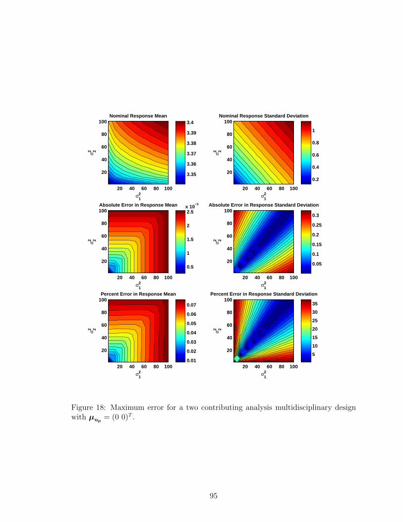
σ12
σ 22
Nominal Response Mean
20 40 60 80 100
20
40
60
80
100
3.35
3.36
3.37
3.38
3.39
3.4
σ12
σ 22
Nominal Response Standard Deviation
20 40 60 80 100
20
40
60
80
100
0.2
0.4
0.6
0.8
1
σ12
σ 22
Absolute Error in Response Mean
20 40 60 80 100
20
40
60
80
100
0.5
1
1.5
2
2.5x 10
−3
σ12
σ 22
Absolute Error in Response Standard Deviation
20 40 60 80 100
20
40
60
80
100
0.05
0.1
0.15
0.2
0.25
0.3
σ12
σ 22
Percent Error in Response Mean
20 40 60 80 100
20
40
60
80
100
0.01
0.02
0.03
0.04
0.05
0.06
0.07
σ12
σ 22
Percent Error in Response Standard Deviation
20 40 60 80 100
20
40
60
80
100
5
10
15
20
25
30
35
Figure 18: Maximum error for a two contributing analysis multidisciplinary designwith µup
= (0 0)T .
95
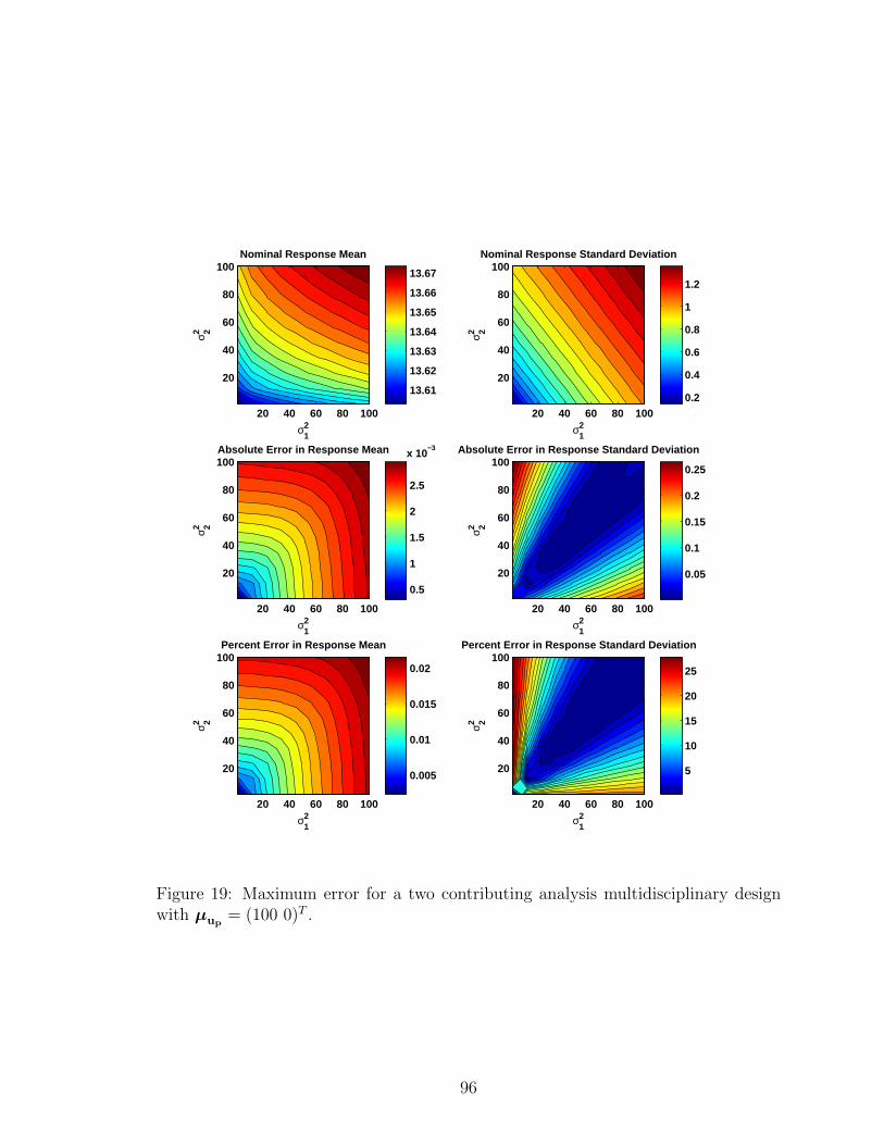
σ12
σ 22
Nominal Response Mean
20 40 60 80 100
20
40
60
80
100
13.61
13.62
13.63
13.64
13.65
13.66
13.67
σ12
σ 22
Nominal Response Standard Deviation
20 40 60 80 100
20
40
60
80
100
0.2
0.4
0.6
0.8
1
1.2
σ12
σ 22
Absolute Error in Response Mean
20 40 60 80 100
20
40
60
80
100
0.5
1
1.5
2
2.5
x 10−3
σ12
σ 22
Absolute Error in Response Standard Deviation
20 40 60 80 100
20
40
60
80
100
0.05
0.1
0.15
0.2
0.25
σ12
σ 22
Percent Error in Response Mean
20 40 60 80 100
20
40
60
80
100
0.005
0.01
0.015
0.02
σ12
σ 22
Percent Error in Response Standard Deviation
20 40 60 80 100
20
40
60
80
100
5
10
15
20
25
Figure 19: Maximum error for a two contributing analysis multidisciplinary designwith µup
= (100 0)T .
96

σ12
σ 22
Nominal Response Mean
20 40 60 80 100
20
40
60
80
100
26.9
26.92
26.94
26.96
26.98
σ12
σ 22
Nominal Response Standard Deviation
20 40 60 80 100
20
40
60
80
100
0.5
1
1.5
σ12
σ 22
Absolute Error in Response Mean
20 40 60 80 100
20
40
60
80
100
0.5
1
1.5
2
2.5
3
x 10−3
σ12
σ 22
Absolute Error in Response Standard Deviation
20 40 60 80 100
20
40
60
80
100
0.05
0.1
0.15
0.2
σ12
σ 22
Percent Error in Response Mean
20 40 60 80 100
20
40
60
80
100
2
4
6
8
10
12
x 10−3
σ12
σ 22
Percent Error in Response Standard Deviation
20 40 60 80 100
20
40
60
80
100
5
10
15
Figure 20: Maximum error for a two contributing analysis multidisciplinary designwith µup
= (100 100)T .
97
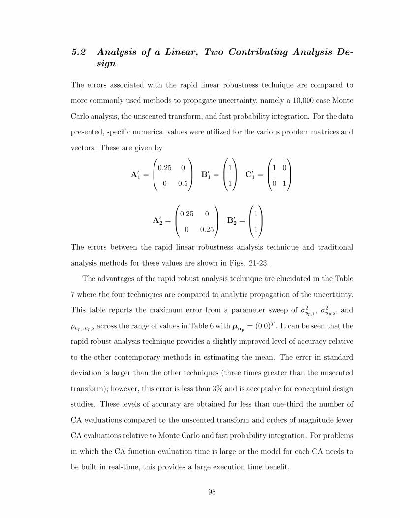
5.2 Analysis of a Linear, Two Contributing Analysis De-sign
The errors associated with the rapid linear robustness technique are compared to
more commonly used methods to propagate uncertainty, namely a 10,000 case Monte
Carlo analysis, the unscented transform, and fast probability integration. For the data
presented, specific numerical values were utilized for the various problem matrices and
vectors. These are given by
A′1 =
0.25 0
0 0.5
B′1 =
1
1
C′1 =
1 0
0 1
A′2 =
0.25 0
0 0.25
B′2 =
1
1
The errors between the rapid linear robustness analysis technique and traditional
analysis methods for these values are shown in Figs. 21-23.
The advantages of the rapid robust analysis technique are elucidated in the Table
7 where the four techniques are compared to analytic propagation of the uncertainty.
This table reports the maximum error from a parameter sweep of σ2up,1
, σ2up,2
, and
ρup,1up,2 across the range of values in Table 6 with µup= (0 0)T . It can be seen that the
rapid robust analysis technique provides a slightly improved level of accuracy relative
to the other contemporary methods in estimating the mean. The error in standard
deviation is larger than the other techniques (three times greater than the unscented
transform); however, this error is less than 3% and is acceptable for conceptual design
studies. These levels of accuracy are obtained for less than one-third the number of
CA evaluations compared to the unscented transform and orders of magnitude fewer
CA evaluations relative to Monte Carlo and fast probability integration. For problems
in which the CA function evaluation time is large or the model for each CA needs to
be built in real-time, this provides a large execution time benefit.
98
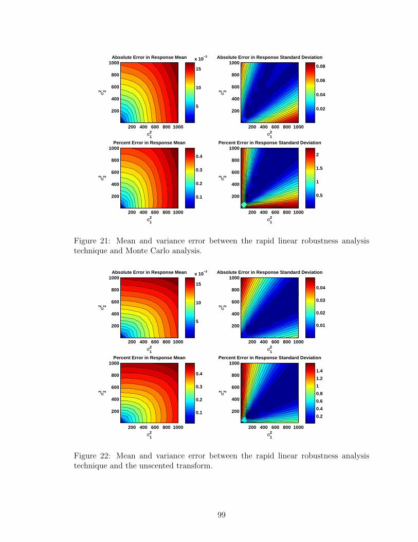
σ12
σ 22
Absolute Error in Response Mean
200 400 600 800 1000
200
400
600
800
1000
5
10
15
x 10−3
σ12
σ 22
Absolute Error in Response Standard Deviation
200 400 600 800 1000
200
400
600
800
1000
0.02
0.04
0.06
0.08
σ12
σ 22
Percent Error in Response Mean
200 400 600 800 1000
200
400
600
800
1000
0.1
0.2
0.3
0.4
σ12
σ 22
Percent Error in Response Standard Deviation
200 400 600 800 1000
200
400
600
800
1000
0.5
1
1.5
2
Figure 21: Mean and variance error between the rapid linear robustness analysistechnique and Monte Carlo analysis.
σ12
σ 22
Absolute Error in Response Mean
200 400 600 800 1000
200
400
600
800
1000
5
10
15
x 10−3
σ12
σ 22
Absolute Error in Response Standard Deviation
200 400 600 800 1000
200
400
600
800
1000
0.01
0.02
0.03
0.04
σ12
σ 22
Percent Error in Response Mean
200 400 600 800 1000
200
400
600
800
1000
0.1
0.2
0.3
0.4
σ12
σ 22
Percent Error in Response Standard Deviation
200 400 600 800 1000
200
400
600
800
1000
0.2
0.4
0.6
0.8
1
1.2
1.4
Figure 22: Mean and variance error between the rapid linear robustness analysistechnique and the unscented transform.
99
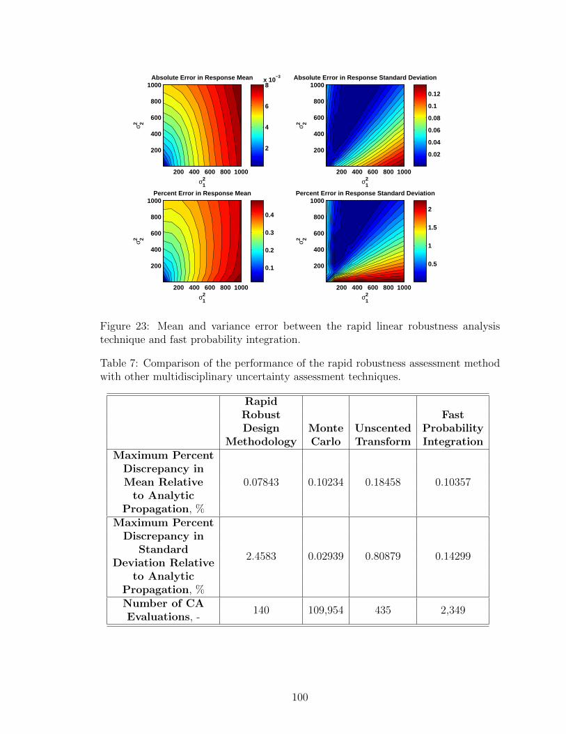
σ12
σ 22
Absolute Error in Response Mean
200 400 600 800 1000
200
400
600
800
1000
2
4
6
8x 10
−3
σ12
σ 22
Absolute Error in Response Standard Deviation
200 400 600 800 1000
200
400
600
800
1000
0.02
0.04
0.06
0.08
0.1
0.12
σ12
σ 22
Percent Error in Response Mean
200 400 600 800 1000
200
400
600
800
1000
0.1
0.2
0.3
0.4
σ12
σ 22
Percent Error in Response Standard Deviation
200 400 600 800 1000
200
400
600
800
1000
0.5
1
1.5
2
Figure 23: Mean and variance error between the rapid linear robustness analysistechnique and fast probability integration.
Table 7: Comparison of the performance of the rapid robustness assessment methodwith other multidisciplinary uncertainty assessment techniques.
RapidRobust FastDesign Monte Unscented Probability
Methodology Carlo Transform IntegrationMaximum Percent
0.07843 0.10234 0.18458 0.10357Discrepancy inMean Relative
to AnalyticPropagation, %
Maximum Percent
2.4583 0.02939 0.80879 0.14299
Discrepancy inStandard
Deviation Relativeto Analytic
Propagation, %Number of CA
140 109,954 435 2,349Evaluations, -
100
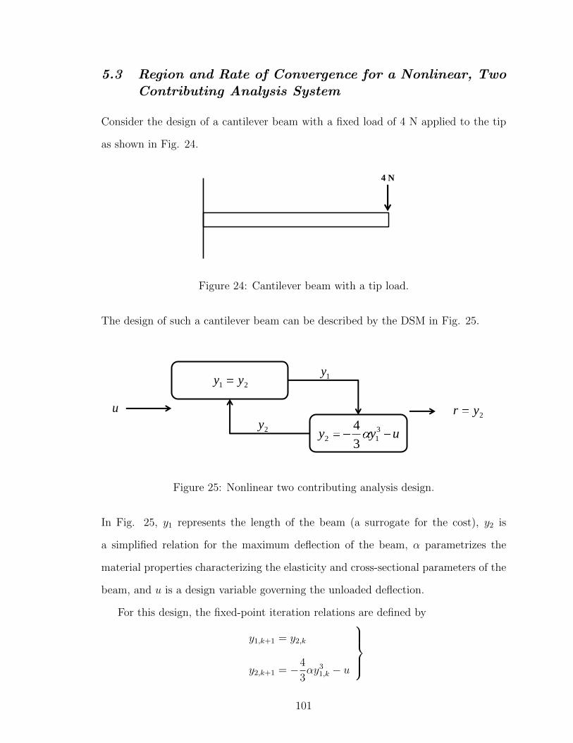
5.3 Region and Rate of Convergence for a Nonlinear, TwoContributing Analysis System
Consider the design of a cantilever beam with a fixed load of 4 N applied to the tip
as shown in Fig. 24.
4 N
Figure 24: Cantilever beam with a tip load.
The design of such a cantilever beam can be described by the DSM in Fig. 25.
21 yy
uyy 3
123
42yru
1y
2y
Figure 25: Nonlinear two contributing analysis design.
In Fig. 25, y1 represents the length of the beam (a surrogate for the cost), y2 is
a simplified relation for the maximum deflection of the beam, α parametrizes the
material properties characterizing the elasticity and cross-sectional parameters of the
beam, and u is a design variable governing the unloaded deflection.
For this design, the fixed-point iteration relations are defined by
y1,k+1 = y2,k
y2,k+1 = −4
3αy3
1,k − u
101
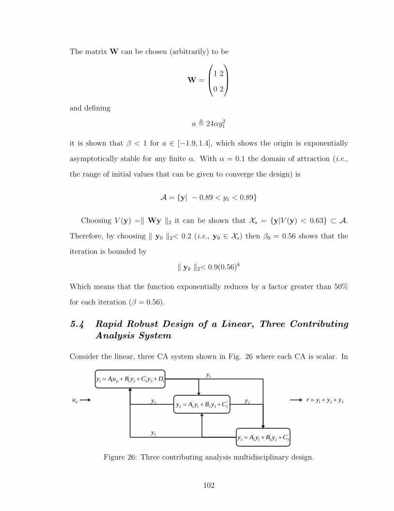
The matrix W can be chosen (arbitrarily) to be
W =
1 2
0 2
and defining
a , 24αy21
it is shown that β < 1 for a ∈ [−1.9, 1.4], which shows the origin is exponentially
asymptotically stable for any finite α. With α = 0.1 the domain of attraction (i.e.,
the range of initial values that can be given to converge the design) is
A = y| − 0.89 < y1 < 0.89
Choosing V (y) =‖ Wy ‖2 it can be shown that Xs = y|V (y) < 0.63 ⊂ A.
Therefore, by choosing ‖ y0 ‖2< 0.2 (i.e., y0 ∈ Xs) then β0 = 0.56 shows that the
iteration is bounded by
‖ yk ‖2< 0.9(0.56)k
Which means that the function exponentially reduces by a factor greater than 50%
for each iteration (β = 0.56).
5.4 Rapid Robust Design of a Linear, Three ContributingAnalysis System
Consider the linear, three CA system shown in Fig. 26 where each CA is scalar. In
'''
p
' DyCyBuAy 1312111
'
232122 CyByAy '' 321 yyyr du
1y
2y
'
323133 CyByAy '' 3y
2y
Figure 26: Three contributing analysis multidisciplinary design.
102
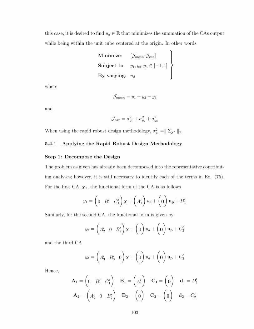
this case, it is desired to find ud ∈ R that minimizes the summation of the CAs output
while being within the unit cube centered at the origin. In other words
Minimize: [Jmean Jvar]
Subject to: y1, y2, y3 ∈ [−1, 1]
By varying: ud
where
Jmean = y1 + y2 + y3
and
Jvar = σ2y1
+ σ2y2
+ σ2y3
When using the rapid robust design methodology, σ2yi
=‖ Σy∗ ‖2.
5.4.1 Applying the Rapid Robust Design Methodology
Step 1: Decompose the Design
The problem as given has already been decomposed into the representative contribut-
ing analyses; however, it is still necessary to identify each of the terms in Eq. (75).
For the first CA, y1, the functional form of the CA is as follows
y1 =
(0 B′1 C ′1
)y +
(A′1
)ud +
(0
)up +D′1
Similarly, for the second CA, the functional form is given by
y2 =
(A′2 0 B′2
)y +
(0
)ud +
(0
)up + C ′2
and the third CA
y3 =
(A′3 B′3 0
)y +
(0
)ud +
(0
)up + C ′3
Hence,
A1 =
(0 B′1 C ′1
)B1 =
(A′1
)C1 =
(0
)d1 = D′1
A2 =
(A′2 0 B′2
)B2 =
(0
)C2 =
(0
)d2 = C ′2
103
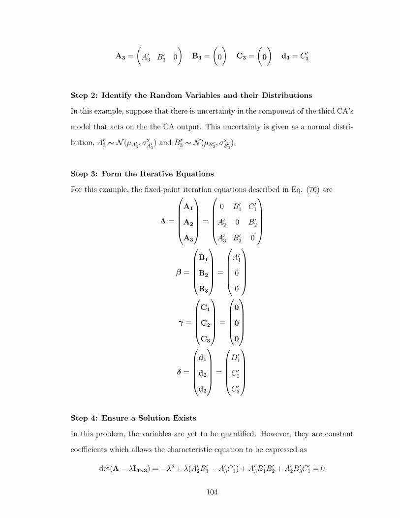
A3 =
(A′3 B′3 0
)B3 =
(0
)C3 =
(0
)d3 = C ′3
Step 2: Identify the Random Variables and their Distributions
In this example, suppose that there is uncertainty in the component of the third CA’s
model that acts on the the CA output. This uncertainty is given as a normal distri-
bution, A′3 ∼ N (µA′3 , σ2A′3
) and B′3 ∼ N (µB′3 , σ2B′3
).
Step 3: Form the Iterative Equations
For this example, the fixed-point iteration equations described in Eq. (76) are
Λ =
A1
A2
A3
=
0 B′1 C ′1
A′2 0 B′2
A′3 B′3 0
β =
B1
B2
B3
=
A′1
0
0
γ =
C1
C2
C3
=
0
0
0
δ =
d1
d2
d2
=
D′1
C ′2
C ′3
Step 4: Ensure a Solution Exists
In this problem, the variables are yet to be quantified. However, they are constant
coefficients which allows the characteristic equation to be expressed as
det(Λ− λI3×3) = −λ3 + λ(A′2B′1 − A′3C ′1) + A′3B
′1B′2 + A′2B
′3C′1 = 0
104
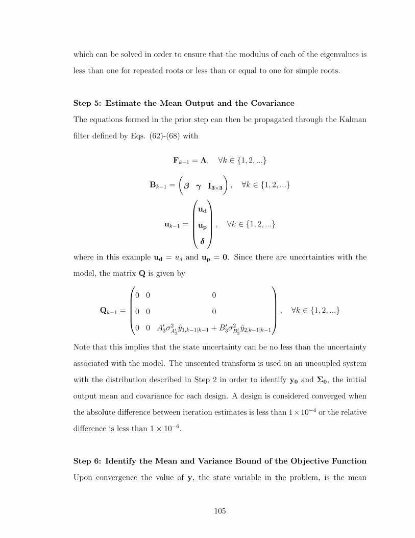
which can be solved in order to ensure that the modulus of each of the eigenvalues is
less than one for repeated roots or less than or equal to one for simple roots.
Step 5: Estimate the Mean Output and the Covariance
The equations formed in the prior step can then be propagated through the Kalman
filter defined by Eqs. (62)-(68) with
Fk−1 = Λ, ∀k ∈ 1, 2, ...
Bk−1 =
(β γ I3×3
), ∀k ∈ 1, 2, ...
uk−1 =
ud
up
δ
, ∀k ∈ 1, 2, ...
where in this example ud = ud and up = 0. Since there are uncertainties with the
model, the matrix Q is given by
Qk−1 =
0 0 0
0 0 0
0 0 A′3σ2A′3y1,k−1|k−1 +B′3σ
2B′3y2,k−1|k−1
, ∀k ∈ 1, 2, ...
Note that this implies that the state uncertainty can be no less than the uncertainty
associated with the model. The unscented transform is used on an uncoupled system
with the distribution described in Step 2 in order to identify y0 and Σ0, the initial
output mean and covariance for each design. A design is considered converged when
the absolute difference between iteration estimates is less than 1×10⁻⁴ or the relative
difference is less than 1× 10⁻⁶.
Step 6: Identify the Mean and Variance Bound of the Objective Function
Upon convergence the value of y, the state variable in the problem, is the mean
105
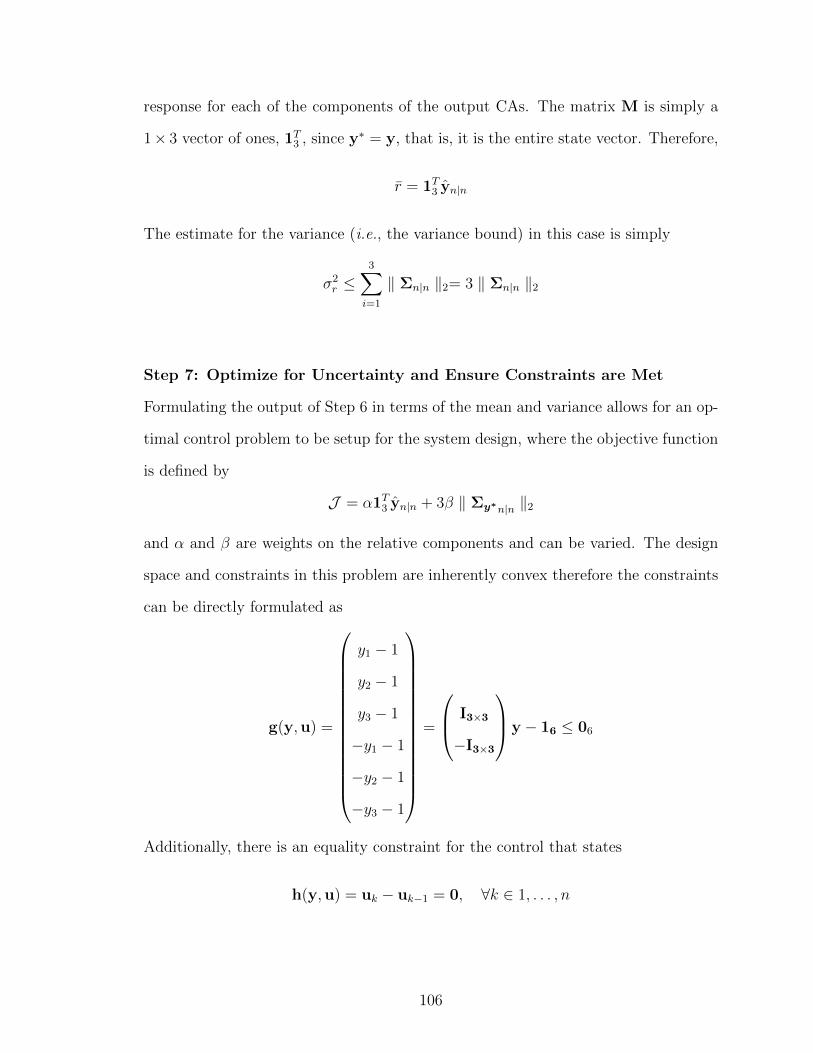
response for each of the components of the output CAs. The matrix M is simply a
1× 3 vector of ones, 1T3 , since y∗ = y, that is, it is the entire state vector. Therefore,
r = 1T3 yn|n
The estimate for the variance (i.e., the variance bound) in this case is simply
σ2r ≤
3∑i=1
‖ Σn|n ‖2= 3 ‖ Σn|n ‖2
Step 7: Optimize for Uncertainty and Ensure Constraints are Met
Formulating the output of Step 6 in terms of the mean and variance allows for an op-
timal control problem to be setup for the system design, where the objective function
is defined by
J = α1T3 yn|n + 3β ‖ Σy∗n|n ‖2
and α and β are weights on the relative components and can be varied. The design
space and constraints in this problem are inherently convex therefore the constraints
can be directly formulated as
g(y,u) =
y1 − 1
y2 − 1
y3 − 1
−y1 − 1
−y2 − 1
−y3 − 1
=
I3×3
−I3×3
y − 16 ≤ 06
Additionally, there is an equality constraint for the control that states
h(y,u) = uk − uk−1 = 0, ∀k ∈ 1, . . . , n
106
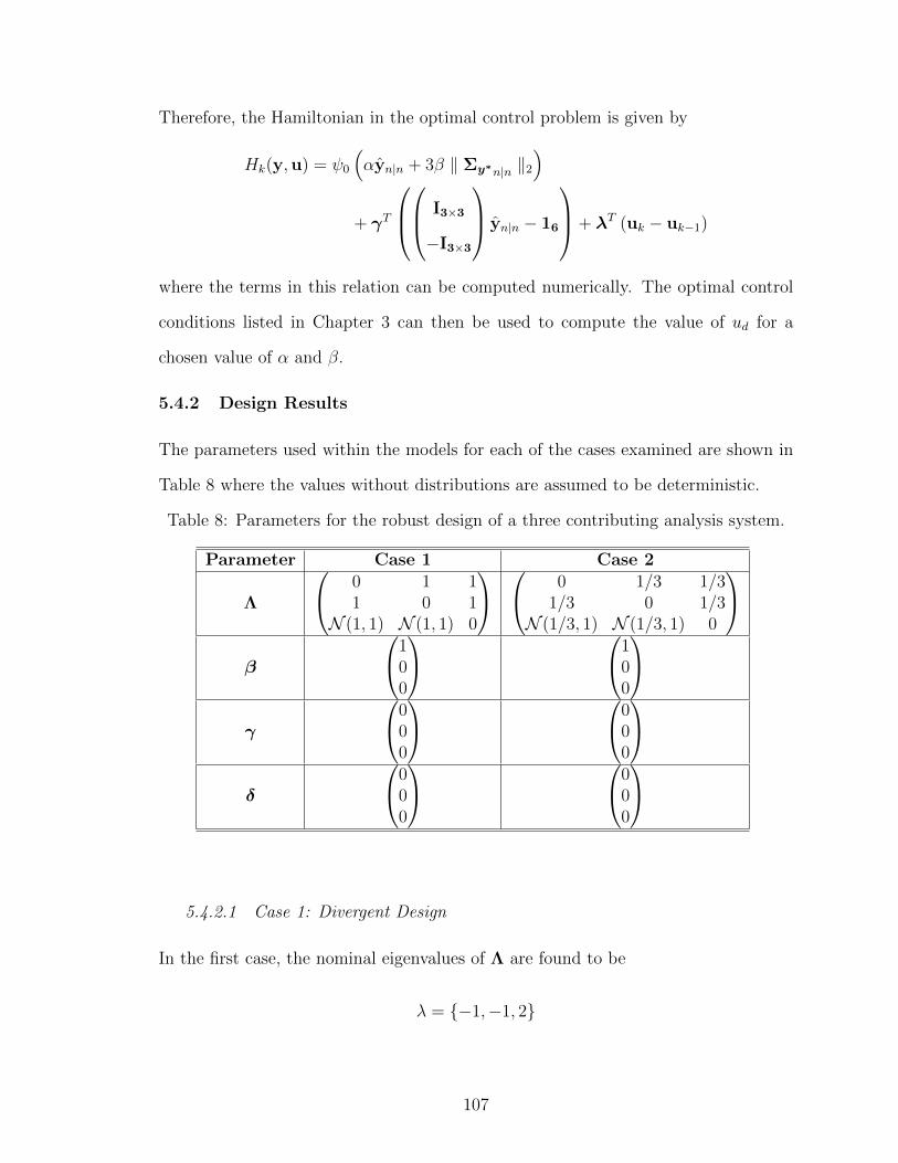
Therefore, the Hamiltonian in the optimal control problem is given by
Hk(y,u) = ψ0
(αyn|n + 3β ‖ Σy∗n|n ‖2
)+ γT
I3×3
−I3×3
yn|n − 16
+ λT (uk − uk−1)
where the terms in this relation can be computed numerically. The optimal control
conditions listed in Chapter 3 can then be used to compute the value of ud for a
chosen value of α and β.
5.4.2 Design Results
The parameters used within the models for each of the cases examined are shown in
Table 8 where the values without distributions are assumed to be deterministic.
Table 8: Parameters for the robust design of a three contributing analysis system.
Parameter Case 1 Case 2
Λ
0 1 11 0 1
N (1, 1) N (1, 1) 0
0 1/3 1/31/3 0 1/3
N (1/3, 1) N (1/3, 1) 0
β
100
100
γ
000
000
δ
000
000
5.4.2.1 Case 1: Divergent Design
In the first case, the nominal eigenvalues of Λ are found to be
λ = −1,−1, 2
107

Hence, since |λmax| ≥ 1 ∀λi, i ∈ 1, 2, 3 there is not a feasible design to be found
with the iteration scheme. This is shown in Fig. 27 where the objective function
value exponentially diverges. Despite fixed-point iteration not being able to find a
1 2 3 4 5 6 7 8 9 100
100
200y i, −
Iteration number, −1 2 3 4 5 6 7 8 9 10
0
500
1000
R =
y1 +
y2 +
y3, −
Figure 27: Divergent behavior demonstrated by the fixed-point iteration system (ud =1).
solution, a feasible design does exist. The feasible designs are characterized by the
equation
y =
0
−1/2
−1/2
ud
which implies that the deterministic optimum is found with ud = 2 which is also the
robust optimum for this problem for an equally weighted objective function. This
example demonstrates the need for alternative iteration schemes to be investigated.
However, it should be noted that the conditions outlined in Chapter 3 accurately
describe the behavior of the dynamical system resulting from the multidisciplinary
design as outlined.
108
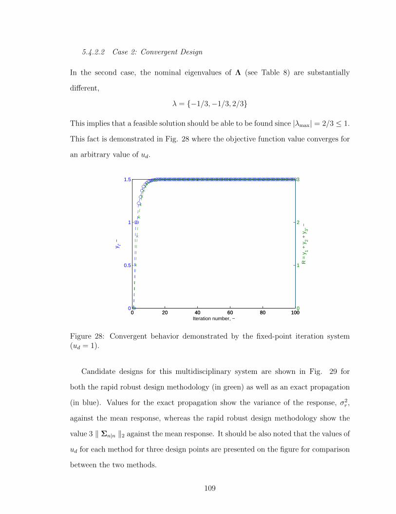
5.4.2.2 Case 2: Convergent Design
In the second case, the nominal eigenvalues of Λ (see Table 8) are substantially
different,
λ = −1/3,−1/3, 2/3
This implies that a feasible solution should be able to be found since |λmax| = 2/3 ≤ 1.
This fact is demonstrated in Fig. 28 where the objective function value converges for
an arbitrary value of ud.
0 20 40 60 80 1000
0.5
1
1.5
y i, −
Iteration number, −0 20 40 60 80 100
0
1
2
3
R =
y1 +
y2 +
y3, −
Figure 28: Convergent behavior demonstrated by the fixed-point iteration system(ud = 1).
Candidate designs for this multidisciplinary system are shown in Fig. 29 for
both the rapid robust design methodology (in green) as well as an exact propagation
(in blue). Values for the exact propagation show the variance of the response, σ2r ,
against the mean response, whereas the rapid robust design methodology show the
value 3 ‖ Σn|n ‖2 against the mean response. It should be also noted that the values of
ud for each method for three design points are presented on the figure for comparison
between the two methods.
109
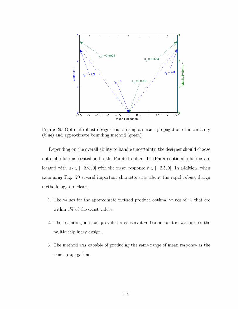
−2.5 −2 −1.5 −1 −0.5 0 0.5 1 1.5 2 2.50
1
2
3
Var
ianc
e, −
Mean Response, −−2.5 −2 −1.5 −1 −0.5 0 0.5 1 1.5 2 2.5
0
1
2
3
Mat
rix 2
−N
orm
, −
ud =−0.6665
ud = 0 u
d =0.0001
ud =0.6664
ud = 2/3
ud = −2/3
Figure 29: Optimal robust designs found using an exact propagation of uncertainty(blue) and approximate bounding method (green).
Depending on the overall ability to handle uncertainty, the designer should choose
optimal solutions located on the the Pareto frontier. The Pareto optimal solutions are
located with ud ∈ [−2/3, 0] with the mean response r ∈ [−2.5, 0]. In addition, when
examining Fig. 29 several important characteristics about the rapid robust design
methodology are clear:
1. The values for the approximate method produce optimal values of ud that are
within 1% of the exact values.
2. The bounding method provided a conservative bound for the variance of the
multidisciplinary design.
3. The method was capable of producing the same range of mean response as the
exact propagation.
110
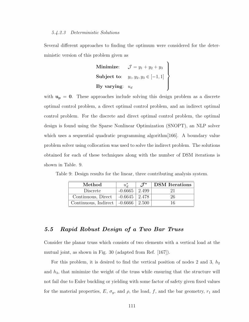
5.4.2.3 Deterministic Solutions
Several different approaches to finding the optimum were considered for the deter-
ministic version of this problem given as
Minimize: J = y1 + y2 + y3
Subject to: y1, y2, y3 ∈ [−1, 1]
By varying: ud
with up = 0. These approaches include solving this design problem as a discrete
optimal control problem, a direct optimal control problem, and an indirect optimal
control problem. For the discrete and direct optimal control problem, the optimal
design is found using the Sparse Nonlinear Optimization (SNOPT), an NLP solver
which uses a sequential quadratic programming algorithm[166]. A boundary value
problem solver using collocation was used to solve the indirect problem. The solutions
obtained for each of these techniques along with the number of DSM iterations is
shown in Table. 9.
Table 9: Design results for the linear, three contributing analysis system.
Method u∗d J ∗ DSM IterationsDiscrete -0.6665 2.499 21
Continuous, Direct -0.6645 2.478 26Continuous, Indirect -0.6666 2.500 16
5.5 Rapid Robust Design of a Two Bar Truss
Consider the planar truss which consists of two elements with a vertical load at the
mutual joint, as shown in Fig. 30 (adapted from Ref. [167]).
For this problem, it is desired to find the vertical position of nodes 2 and 3, h2
and h3, that minimize the weight of the truss while ensuring that the structure will
not fail due to Euler buckling or yielding with some factor of safety given fixed values
for the material properties, E, σy, and ρ, the load, f , and the bar geometry, r1 and
111

x
y
Node 1
(0,0)
Node 2
(x2,y2)
Node 3
(0,y3)
Bar 2
Bar 1
r
Bar
Cross-Section
f
g
l
Figure 30: Two bar truss with a load at the mutual joint.
r2. The horizontal position of node 2 is constrained to be l. In standard form, the
problem is written as
Minimize: [m σ2m]
Subject to: g1(h2, h3) = |T1(h2, h3)| − πr21σy ≤ 0
g2(h2, h3) = |T2(h2, h3)| − πr22σy ≤ 0
g3(h2, h3) = −T1(h2, h3)− π2EI1
L21
≤ 0
g4(h2, h3) = −T2(h2, h3)− π2EI2
L22
≤ 0
By varying: h2, h3
where m is the mean mass of the bars and the variance of the mass, σ2
m, for the rapid
robust design methodology is given by ‖ Σy∗ ‖2. In these relations, the mass is given
by
m = ρπg(r2
1L1 + r22L2
)= ρπg
(r2
1
√l2 + h2
2 + r22
√l2 + (h3 − h2)2
)L1 and L2 are the lengths of the two bars, respectively, I1 and I2 are the moments
of inertia of the two bars (Ii =1
4mr2
i ), and T1(h2, h3) and T2(h2, h3) are the tensions
112
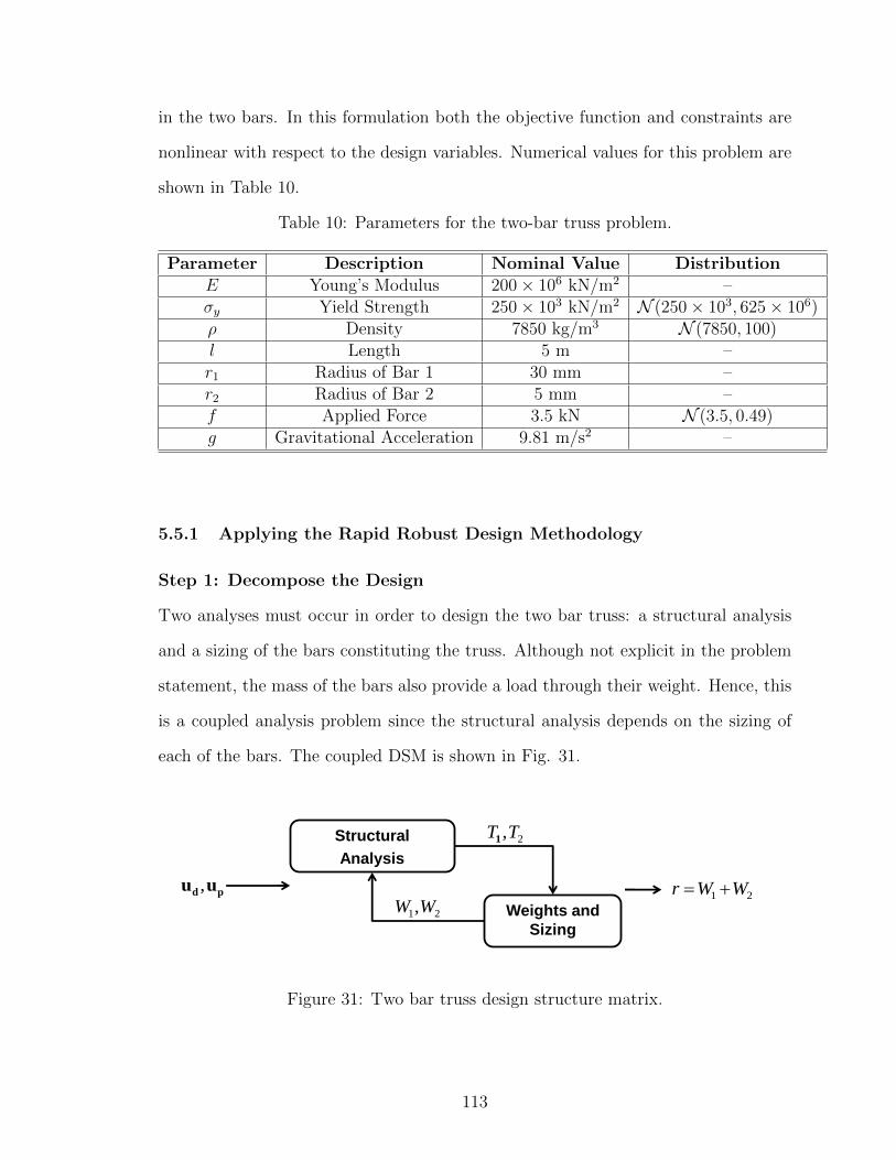
in the two bars. In this formulation both the objective function and constraints are
nonlinear with respect to the design variables. Numerical values for this problem are
shown in Table 10.
Table 10: Parameters for the two-bar truss problem.
Parameter Description Nominal Value DistributionE Young’s Modulus 200× 106 kN/m2 –σy Yield Strength 250× 103 kN/m2 N (250× 103, 625× 106)ρ Density 7850 kg/m3 N (7850, 100)l Length 5 m –r1 Radius of Bar 1 30 mm –r2 Radius of Bar 2 5 mm –f Applied Force 3.5 kN N (3.5, 0.49)g Gravitational Acceleration 9.81 m/s2 –
5.5.1 Applying the Rapid Robust Design Methodology
Step 1: Decompose the Design
Two analyses must occur in order to design the two bar truss: a structural analysis
and a sizing of the bars constituting the truss. Although not explicit in the problem
statement, the mass of the bars also provide a load through their weight. Hence, this
is a coupled analysis problem since the structural analysis depends on the sizing of
each of the bars. The coupled DSM is shown in Fig. 31.
Structural
Analysis
Weights and
Sizing
21 WWr pd uu ,
2,TT1
21,WW
Figure 31: Two bar truss design structure matrix.
113
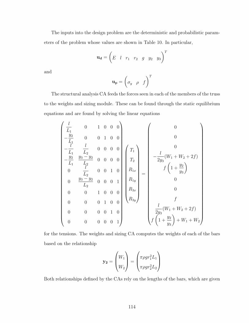
The inputs into the design problem are the deterministic and probabilistic param-
eters of the problem whose values are shown in Table 10. In particular,
ud =
(E l r1 r2 g y2 y3
)Tand
up =
(σy ρ f
)TThe structural analysis CA feeds the forces seen in each of the members of the truss
to the weights and sizing module. These can be found through the static equilibrium
equations and are found by solving the linear equations
l
L1
0 1 0 0 0
− y2
L1
0 0 1 0 0
− l
L1
l
L2
0 0 0 0
− y2
L1
y3 − y2
L2
0 0 0 0
0l
L2
0 0 1 0
0y3 − y2
L2
0 0 0 1
0 0 1 0 0 0
0 0 0 1 0 0
0 0 0 0 1 0
0 0 0 0 0 1
T1
T2
R1x
R1y
R3x
R3y
=
0
0
0
− l
2y3
(W1 +W2 + 2f)
f
(1 +
y2
y3
)0
0
f
l
2y3
(W1 +W2 + 2f)
f
(1 +
y2
y3
)+W1 +W2
for the tensions. The weights and sizing CA computes the weights of each of the bars
based on the relationship
y2 =
W1
W2
=
πρgr21L1
πρgr22L2
Both relationships defined by the CAs rely on the lengths of the bars, which are given
114
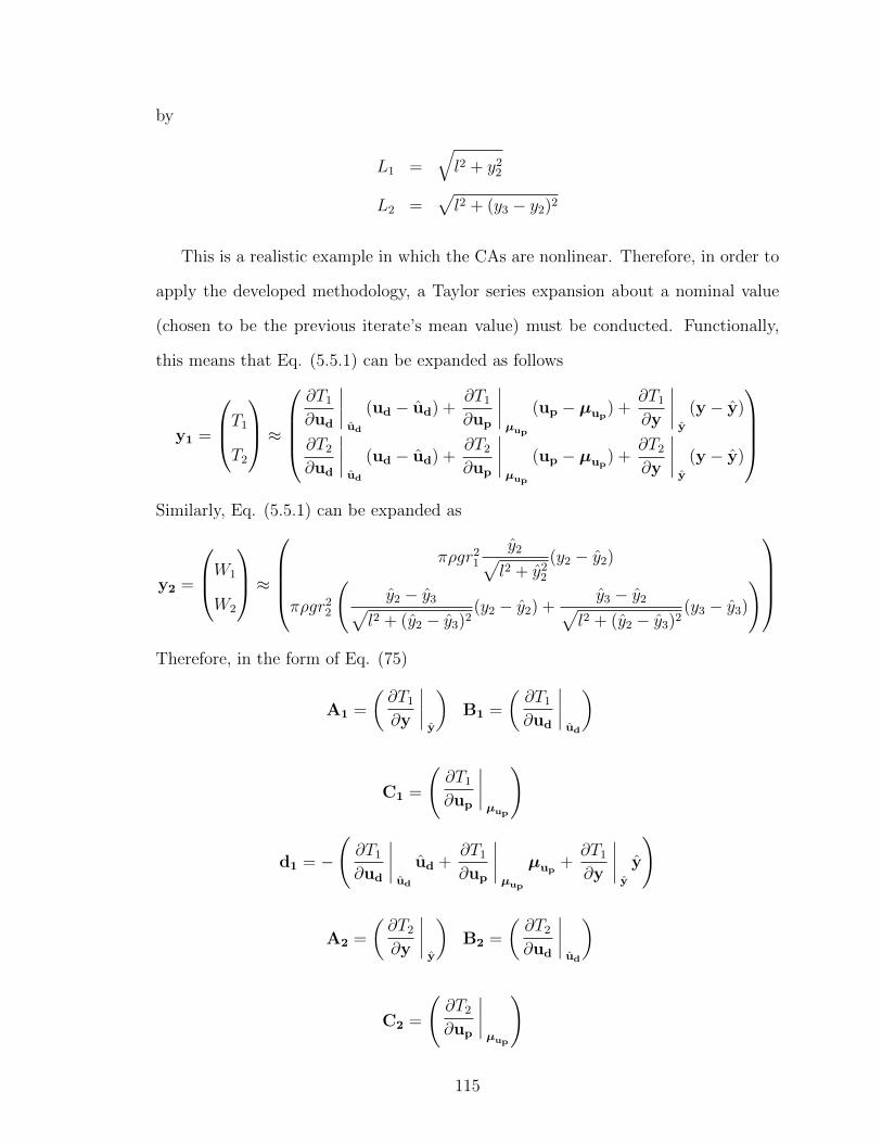
by
L1 =√l2 + y2
2
L2 =√l2 + (y3 − y2)2
This is a realistic example in which the CAs are nonlinear. Therefore, in order to
apply the developed methodology, a Taylor series expansion about a nominal value
(chosen to be the previous iterate’s mean value) must be conducted. Functionally,
this means that Eq. (5.5.1) can be expanded as follows
y1 =
T1
T2
≈∂T1
∂ud
ud
(ud − ud) +∂T1
∂up
µup
(up − µup) +
∂T1
∂y
y
(y − y)
∂T2
∂ud
ud
(ud − ud) +∂T2
∂up
µup
(up − µup) +
∂T2
∂y
y
(y − y)
Similarly, Eq. (5.5.1) can be expanded as
y2 =
W1
W2
≈
πρgr21
y2√l2 + y2
2
(y2 − y2)
πρgr22
(y2 − y3√
l2 + (y2 − y3)2(y2 − y2) +
y3 − y2√l2 + (y2 − y3)2
(y3 − y3)
)
Therefore, in the form of Eq. (75)
A1 =
(∂T1
∂y
y
)B1 =
(∂T1
∂ud
ud
)
C1 =
(∂T1
∂up
µup
)
d1 = −
(∂T1
∂ud
ud
ud +∂T1
∂up
µup
µup+∂T1
∂y
y
y
)
A2 =
(∂T2
∂y
y
)B2 =
(∂T2
∂ud
ud
)
C2 =
(∂T2
∂up
µup
)
115

d2 = −
(∂T2
∂ud
ud
ud +∂T2
∂up
µup
µup+∂T2
∂y
y
y
)
Step 2: Identify the Random Variables and their Distributions
All of the random variables in this example are associated with the parameters
and not with the model itself. As shown in Table 10, the values are given by
σy ∼ N (250× 103, 625× 106), ρ ∼ N (7850, 100), and f ∼ N (3.5, 0.49).
Step 3: Form the Iterative Equations
In order to use the Kalman filter to simultaneously estimate robustness and converge
the design, the iterative equations described in Eq. (76) for fixed-point iteration need
to be formed. Through analogy of variables, the matrices are given by
Λ =
A1
A2
=
0∂T1
∂y2
y
∂T2
∂y1
y
0
β =
B1
B2
=
∂T1
∂ud
ud
∂T2
∂ud
ud
γ =
C1
C2
=
∂T1
∂up
µup
∂T2
∂up
µup
δ =
d1
d2
=
−
(∂T1
∂ud
ud
ud +∂T1
∂up
µup
µup+∂T1
∂y
y
y
)
−
(∂T2
∂ud
ud
ud +∂T2
∂up
µup
µup+∂T2
∂y
y
y
)
where the numerical values for each of these matrices is evaluated at each subsequent
iteration at the appropriate nominal values.
116
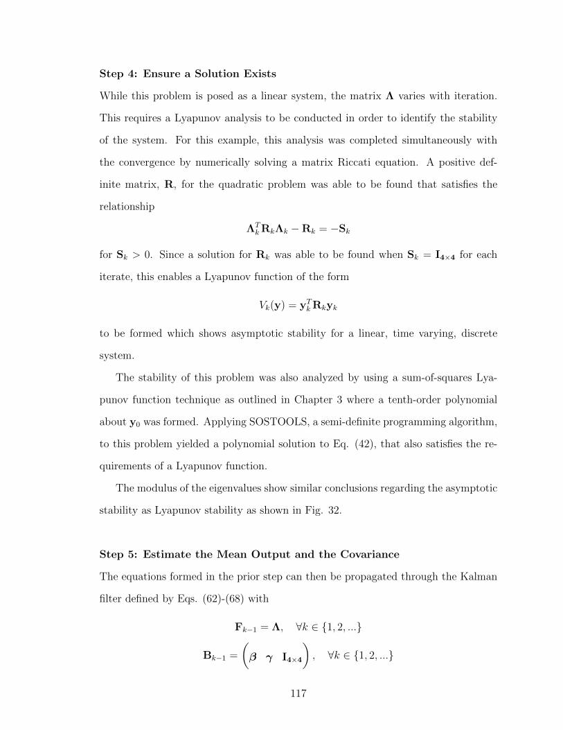
Step 4: Ensure a Solution Exists
While this problem is posed as a linear system, the matrix Λ varies with iteration.
This requires a Lyapunov analysis to be conducted in order to identify the stability
of the system. For this example, this analysis was completed simultaneously with
the convergence by numerically solving a matrix Riccati equation. A positive def-
inite matrix, R, for the quadratic problem was able to be found that satisfies the
relationship
ΛTkRkΛk −Rk = −Sk
for Sk > 0. Since a solution for Rk was able to be found when Sk = I4×4 for each
iterate, this enables a Lyapunov function of the form
Vk(y) = yTk Rkyk
to be formed which shows asymptotic stability for a linear, time varying, discrete
system.
The stability of this problem was also analyzed by using a sum-of-squares Lya-
punov function technique as outlined in Chapter 3 where a tenth-order polynomial
about y0 was formed. Applying SOSTOOLS, a semi-definite programming algorithm,
to this problem yielded a polynomial solution to Eq. (42), that also satisfies the re-
quirements of a Lyapunov function.
The modulus of the eigenvalues show similar conclusions regarding the asymptotic
stability as Lyapunov stability as shown in Fig. 32.
Step 5: Estimate the Mean Output and the Covariance
The equations formed in the prior step can then be propagated through the Kalman
filter defined by Eqs. (62)-(68) with
Fk−1 = Λ, ∀k ∈ 1, 2, ...
Bk−1 =
(β γ I4×4
), ∀k ∈ 1, 2, ...
117

0 5 10 15 20 250.55
0.6
0.65
0.7
0.75
0.8
0.85
0.9
Iteration Number, −
Max
imum
Eig
enva
lue
Mod
ulus
, −
Figure 32: History of the modulus of the maximum eigenvalue of the two bar trusssystem with iteration.
uk−1 =
ud
up
δ
, ∀k ∈ 1, 2, ...
where in this example ud =
(E l r1 r2 g y2 y3
)Tand up = E(up) = µup
. In
this example, the matrix Q is the null matrix since the only uncertain parameters of
the problem are associated with the input parameters, not the model. The unscented
transform is used on an uncoupled system with the distribution described in Step 2
in order to identify y0 and Σ0, the initial output mean and covariance for each de-
sign. A design is considered converged when the absolute difference between iteration
estimates is less than 1× 10⁻⁴ or the relative difference is less than 1× 10⁻⁶.
Step 6: Identify the Mean and Variance Bound of the Objective Function
Upon convergence, the value of y, the state variable in the problem, is the mean
response for each of the components of the output CAs. In this example, the matrix
118
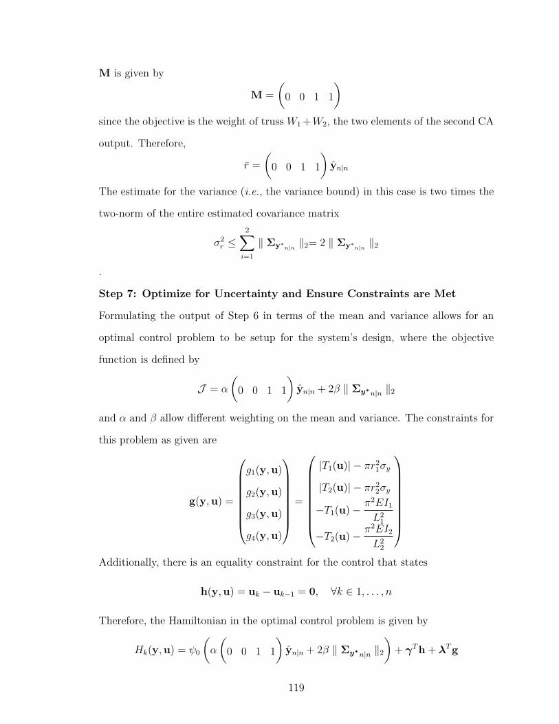
M is given by
M =
(0 0 1 1
)since the objective is the weight of truss W1 +W2, the two elements of the second CA
output. Therefore,
r =
(0 0 1 1
)yn|n
The estimate for the variance (i.e., the variance bound) in this case is two times the
two-norm of the entire estimated covariance matrix
σ2r ≤
2∑i=1
‖ Σy∗n|n ‖2= 2 ‖ Σy∗n|n ‖2
.
Step 7: Optimize for Uncertainty and Ensure Constraints are Met
Formulating the output of Step 6 in terms of the mean and variance allows for an
optimal control problem to be setup for the system’s design, where the objective
function is defined by
J = α
(0 0 1 1
)yn|n + 2β ‖ Σy∗n|n ‖2
and α and β allow different weighting on the mean and variance. The constraints for
this problem as given are
g(y,u) =
g1(y,u)
g2(y,u)
g3(y,u)
g4(y,u)
=
|T1(u)| − πr21σy
|T2(u)| − πr22σy
−T1(u)− π2EI1
L21
−T2(u)− π2EI2
L22
Additionally, there is an equality constraint for the control that states
h(y,u) = uk − uk−1 = 0, ∀k ∈ 1, . . . , n
Therefore, the Hamiltonian in the optimal control problem is given by
Hk(y,u) = ψ0
(α
(0 0 1 1
)yn|n + 2β ‖ Σy∗n|n ‖2
)+ γTh + λTg
119
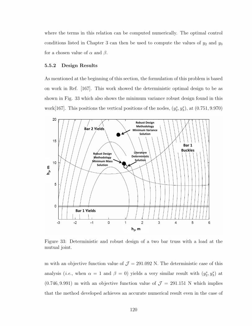
where the terms in this relation can be computed numerically. The optimal control
conditions listed in Chapter 3 can then be used to compute the values of y2 and y3
for a chosen value of α and β.
5.5.2 Design Results
As mentioned at the beginning of this section, the formulation of this problem is based
on work in Ref. [167]. This work showed the deterministic optimal design to be as
shown in Fig. 33 which also shows the minimum variance robust design found in this
work[167]. This positions the vertical positions of the nodes, (y∗2, y∗3), at (0.751, 9.970)
Bar 1 Yields
h2, m
h3, m
Literature Deterministic
Solution
Bar 2 Yields
Bar 1 Buckles
Robust Design Methodology
Minimum Mass Solution
Robust Design Methodology
Minimum Variance Solution
Figure 33: Deterministic and robust design of a two bar truss with a load at themutual joint.
m with an objective function value of J = 291.092 N. The deterministic case of this
analysis (i.e., when α = 1 and β = 0) yields a very similar result with (y∗2, y∗3) at
(0.746, 9.991) m with an objective function value of J = 291.151 N which implies
that the method developed achieves an accurate numerical result even in the case of
120
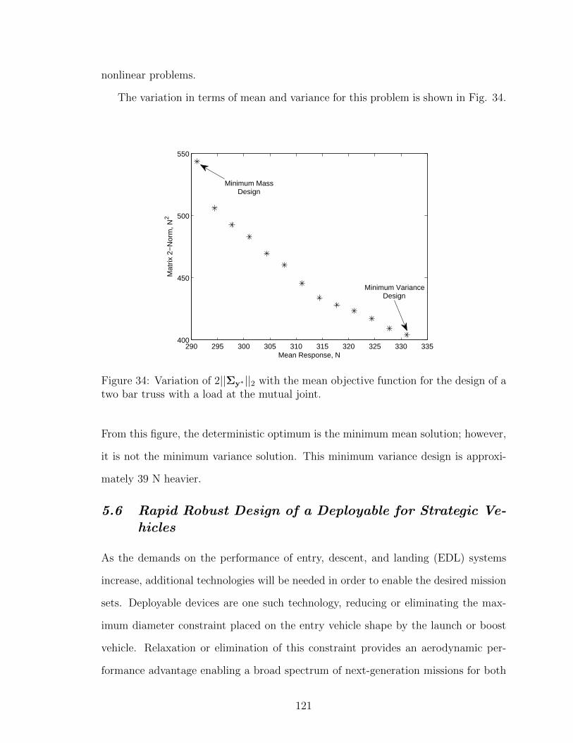
nonlinear problems.
The variation in terms of mean and variance for this problem is shown in Fig. 34.
290 295 300 305 310 315 320 325 330 335400
450
500
550
Mean Response, N
Mat
rix 2
−N
orm
, N2
Minimum MassDesign
Minimum VarianceDesign
Figure 34: Variation of 2||Σy∗ ||2 with the mean objective function for the design of atwo bar truss with a load at the mutual joint.
From this figure, the deterministic optimum is the minimum mean solution; however,
it is not the minimum variance solution. This minimum variance design is approxi-
mately 39 N heavier.
5.6 Rapid Robust Design of a Deployable for Strategic Ve-hicles
As the demands on the performance of entry, descent, and landing (EDL) systems
increase, additional technologies will be needed in order to enable the desired mission
sets. Deployable devices are one such technology, reducing or eliminating the max-
imum diameter constraint placed on the entry vehicle shape by the launch or boost
vehicle. Relaxation or elimination of this constraint provides an aerodynamic per-
formance advantage enabling a broad spectrum of next-generation missions for both
121
civilian and national defense applications. Some examples of previously investigated
deployable systems are discussed in Refs. [168, 169, 170, 171, 172, 173, 174, 175, 176,
177, 178, 179, 180, 181, 182].
Deployables are usually thought to be drag enhancing devices to reduce the ballis-
tic coefficient of a system. However, for strategic vehicles, the inclusion of a deployable
device may also improve controllability, enhance constraint margins, and lead to new
concepts of operations. Boost-glide systems are typically mid- to high-L/D systems
that use a boost phase to achieve a desired state and then manage their energy to
glide to their desired target. Deployables could be added to existing strategic systems
leading to an evolved boost-glide mission set through increased range and accuracy.
This work robustly designs deployable systems for a representative strategic system
in order to examine this evolved boost-glide mission set.
5.6.1 Performance Impact of a Deployable System
In general, the performance of a vehicle is strongly characterized by the ballistic
coefficient, β, and the lift-to-drag ratio, L/D [183]. Figure 35 shows the 1σ miss
distance to a surface target and achievable range as a function of L/D for a range of
β. The results seen in Fig. 35 are the product of solving the optimal control problem
where the control is the orientation and magnitude of the net aerodynamic force
vector at Earth from an initial state of h0 = 155 km, v0 = 6.2 km/s, and γ0 = −9.6.
It was assumed that the aerodynamic force vector could be oriented freely and non-
continuously within a reachable cone having a half-angle defined by the maximum
L/D. The objective function to be maximized for this optimization problem is either
accuracy (in the case of Fig. 35(a)) or range (in the case of Fig. 35(b)).
In Fig. 35, it is seen that the miss distance is relatively insensitive to ballistic
coefficient; however, there is a strong, nonlinear dependence on L/D for values less
122
0 0.1 0.2 0.3 0.4 0.5 0.6 0.7 0.8 0.90
5
10
15
20
25
L/D, −
1σ M
iss
Dis
tanc
e, k
m
β = 1 kg/m2
β = 5 kg/m2
β = 10 kg/m2
β = 50 kg/m2
(a)
0 0.5 1 1.5 20
0.2
0.4
0.6
0.8
1
1.2
1.4
1.6
1.8
L/D, −
1σ N
orm
aliz
ed R
ange
, −
β = 1 kg/m2
β = 5 kg/m2
β = 10 kg/m2
β = 50 kg/m2
(b)
Figure 35: Variation of (a) miss distance and (b) range showing sensitivity to lift-to-drag ratio and insensitivity to ballistic coefficient.
123
than 0.3 with limited additional improvement beyond this point. A strong, near-
linear dependence on L/D is seen for range capability. Like with the accuracy, there
is little sensitivity to the ballistic coefficient.
There is a large design space of deployable concepts. This investigation will limit
the design to a single concept—that of deployable chines, which are shown in Fig. 36.
In this investigation, the root chord is fixed at 2d.
d
l
Figure 36: Geometry of the deployable device.
Chines have the potential to increase the L/D performance of the system [184, 185,
186, 187]. This effect is shown in Fig. 37 where the improvement over a representative
baseline’s L/D is plotted against a non-dimensional size, l/d—the ratio of the distance
from the centerline of the vehicle to tip chord of the deployable to the baseline vehicle’s
diameter.
Figure 35 implies that from a performance perspective, the vehicle should have
as much L/D as possible while Fig. 37 indicates that in order to maximize the L/D
of the system, the deployable should be as large as possible. However, the larger the
deployable the more massive it is, which negatively impacts the performance of the
system. Therefore, a multiobjective design problem is formulated where the mass
124
0 0.5 1 1.5 21
1.05
1.1
1.15
1.2
1.25
1.3
l/d, −
(L/D
)/(L
/D) ba
selin
e, −
Figure 37: Increase in the maximum lift-to-drag ratio of the entry system for a single-delta deployable as a function of deployable size.
Table 11: Baseline strategic vehicle aerodynamics
Parameter Value(L/D)max 1.02α|(L/D)max 22.5
CL|(L/D)max 0.864CD|(L/D)max 0.849
of the decelerator is traded with the performance of the system (either accuracy or
range).
5.6.2 Baseline Strategic System Characteristics
The rapid robust design methodology is used to design a deployable system that
could be added to a representative baseline strategic system to potentially improve
its performance. The baseline system is shown in Fig. 38 and selected characteristics
describing its aerodynamics are shown in Table 11.
125
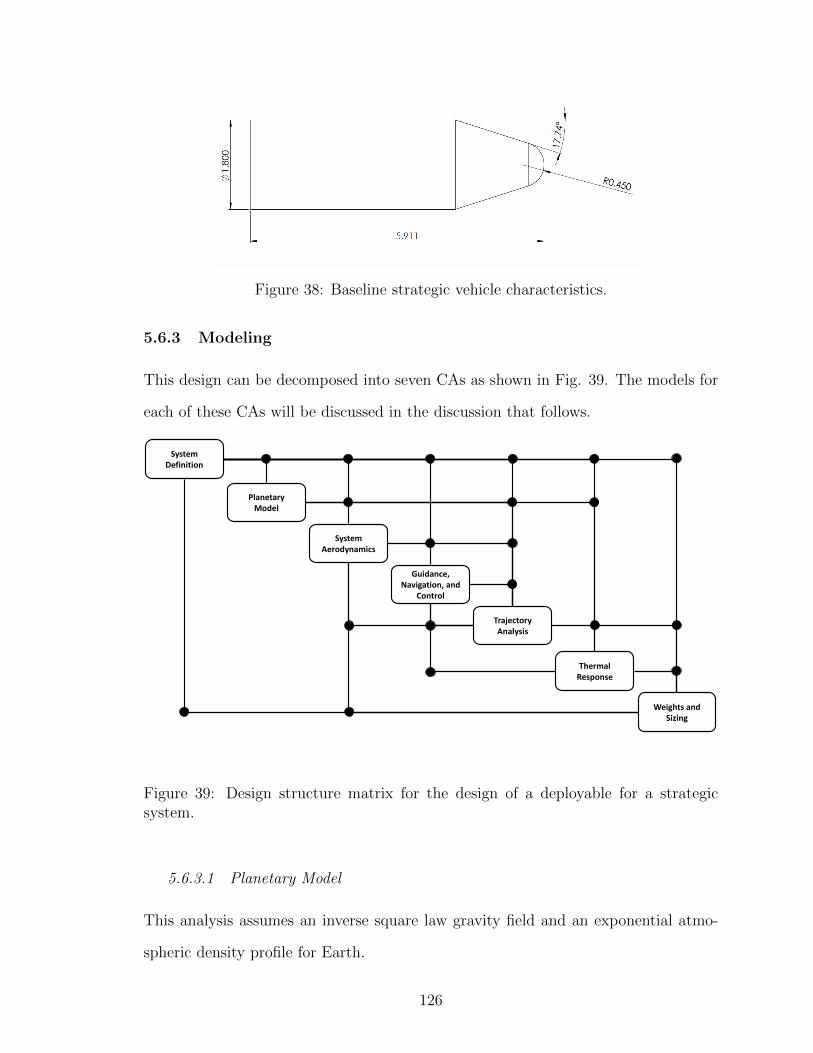
Figure 38: Baseline strategic vehicle characteristics.
5.6.3 Modeling
This design can be decomposed into seven CAs as shown in Fig. 39. The models for
each of these CAs will be discussed in the discussion that follows.
System Definition
Planetary Model
Guidance, Navigation, and
Control
Trajectory Analysis
Thermal Response
Weights and Sizing
System Aerodynamics
Figure 39: Design structure matrix for the design of a deployable for a strategicsystem.
5.6.3.1 Planetary Model
This analysis assumes an inverse square law gravity field and an exponential atmo-
spheric density profile for Earth.
126
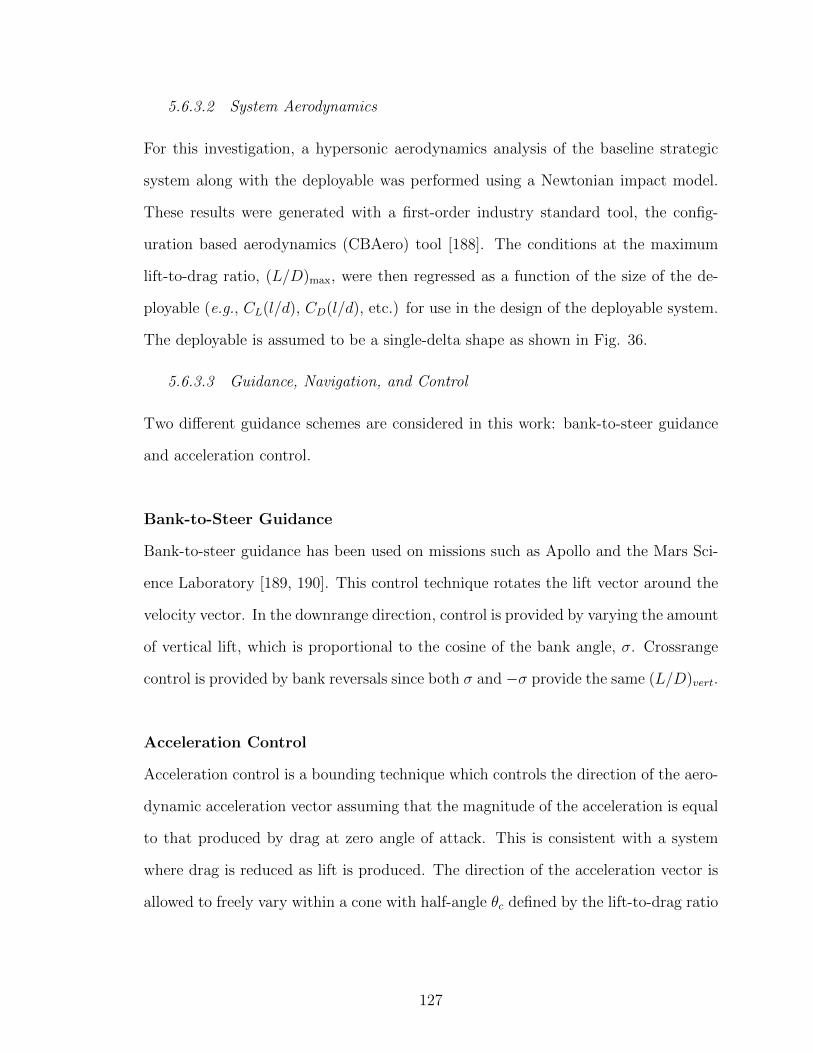
5.6.3.2 System Aerodynamics
For this investigation, a hypersonic aerodynamics analysis of the baseline strategic
system along with the deployable was performed using a Newtonian impact model.
These results were generated with a first-order industry standard tool, the config-
uration based aerodynamics (CBAero) tool [188]. The conditions at the maximum
lift-to-drag ratio, (L/D)max, were then regressed as a function of the size of the de-
ployable (e.g., CL(l/d), CD(l/d), etc.) for use in the design of the deployable system.
The deployable is assumed to be a single-delta shape as shown in Fig. 36.
5.6.3.3 Guidance, Navigation, and Control
Two different guidance schemes are considered in this work: bank-to-steer guidance
and acceleration control.
Bank-to-Steer Guidance
Bank-to-steer guidance has been used on missions such as Apollo and the Mars Sci-
ence Laboratory [189, 190]. This control technique rotates the lift vector around the
velocity vector. In the downrange direction, control is provided by varying the amount
of vertical lift, which is proportional to the cosine of the bank angle, σ. Crossrange
control is provided by bank reversals since both σ and −σ provide the same (L/D)vert.
Acceleration Control
Acceleration control is a bounding technique which controls the direction of the aero-
dynamic acceleration vector assuming that the magnitude of the acceleration is equal
to that produced by drag at zero angle of attack. This is consistent with a system
where drag is reduced as lift is produced. The direction of the acceleration vector is
allowed to freely vary within a cone with half-angle θc defined by the lift-to-drag ratio
127
of the system
θc = tan−1
(L
D
)= tan−1
(CLCD
)(99)
Mathematically, the commanded acceleration is given by
ac =Dmax
mu =
ρv2CD|α=0A
2m
u
‖ u ‖(100)
with the constraint that
cos−1
(uTv
v
)≤ θc (101)
Implementation
During propagation of the trajectory, an optimal control trajectory is obtained for the
remainder of the trajectory at frequency of 0.5 Hz. This optimal control is predicted
using GPOPS, a pseudospectral optimal control software [191, 192, 193, 194, 195]. In
the case where the range is to be maximized, the objective function used in GPOPS
is given by
J = −sf = −s(tf ) (102)
Similarly, when the accuracy is to be maximized, the objective function is given as
J = d2miss = (r(tf )− rT)T (r(tf )− rT) (103)
which is equivalent to minimizing the miss distance.
5.6.3.4 Trajectory Analysis
In addition to Cartesian equations of motion, an additional equation for the range of
the system is also propagated. This equation for the range is given by
s = v cos(γ) (104)
These equations were propagated from the initial state using a fixed-step, fourth-
order, Runge-Kutta propagator until the system reached the surface (h = 0).
128
5.6.3.5 Thermal Response
The Sutton-Graves approximation for stagnation point heating is used [196].
qs = ks
√ρ
rnv3 (105)
For this analysis, rn = 0.25 m and the nominal value of the Sutton-Graves constant,
ks, for Earth, 1.74153× 10⁻⁴ kg1/2m−1/2 is used.
5.6.3.6 Weights and Sizing
Deployable Structure
The sizing of the deployable’s structure is based on work by Krivoshapko for ellipsoidal
shell pressure vessels where analytical relationships for the meridional and parallel
stresses and critical buckling pressure are given in terms of the geometry of the
ellipsoid [197].
σφ =p
2bδ
√r2(b2 − a2) + a4 (106)
σβ =p
2bδ
2r2(b2 − a2) + a4√r2(b2 − a2) + a4
(107)
pcr =16Eδ4
a2√
3(1− ν2)
[1 +
(za
)1/2√
193(1− 4δ2)
16δ√
12(1− ν2)
](108)
In this work, the thickness, δ, is chosen based on minimum thickness resulting from
Eqs. (106), (107), and (108) when a factor of safety of 1.3 is applied. The value of the
internal pressure, p, is chosen such that it is twice the maximum dynamic pressure
experienced. The dimensions of the ellipsoid are such that it produces a minimum
volume deployable. The deployable’s mass is determined by the following relationship
mstructure =3√
3l2zδρd4
(109)
which includes an increase in mass of 50% to account for deployable systems and
design immaturity.
129
Deployable TPS System
A first-order relationship determined by Laub and Venkatapathy uses heat load as
the sole parameter to determine the thermal protection system (TPS) mass fraction
[198]. This approximate relation is used in this investigation to size the TPS material
for the deployable. The model uses historical United States planetary missions at
Venus, Earth, Mars, and Jupiter with ablative TPS to regress TPS mass fraction
against the integrated heat load. These missions have integrated heat loads ranging
from approximately 3 × 10³ J/cm2 to 2 × 10⁵ J/cm2 (the trajectories analyzed in
this investigation have heat loads that are approximately 7-12 × 103 J/cm2). The
derived mass model for the TPS is given by [198]
mTPS =(9.1× 10⁻⁴Q0.51575
)m0 (110)
where Q is the integrated heat load in J/cm2 and m0 is the initial mass.
Deployable Mass
The total deployable’s mass is the addition of the structural mass (including deploy-
able system mass and margin) and the TPS system.
mdeploy = mstructure +mTPS (111)
5.6.4 Problem Setup
The setup of the design problem posed is presented below. First, the parameters
used within the models is presented, then the problem constraints are introduced,
and finally the optimization problem is formed.
5.6.4.1 Design Parameters
The solutions presented subsequently are based on the deterministic and probabilistic
parameters shown in Table 12.
130
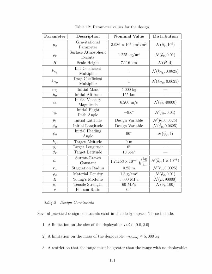
Table 12: Parameter values for the design.
Parameter Description Nominal Value Distribution
µgGravitational
3.986× 10⁵ km3/m2 N (µg, 106)Parameter
ρ0Surface Atmospheric
1.225 kg/m3 N (ρ0, 0.01)Density
H Scale Height 7.116 km N (H, 4)
kCL
Lift Coefficient1 N (kCL
, 0.0625)Multiplier
kCD
Drag Coefficient1 N (kCD
, 0.0625)Multiplier
m0 Initial Mass 5,000 kg —h0 Initial Altitude 155 km —
v0Initial Velocity
6,200 m/s N (v0, 40000)Magnitude
γ0Initial Flight −9.6 N (γ0, 0.04)Path Angle
θ0 Initial Latitude Design Variable N (θ0, 0.0625)
φ0 Initial Longitude Design Variable N (φ0, 0.0625)
ψ0Initial Heading
90 N (ψ0, 4)Angle
hT Target Altitude 0 m —φT Target Longitude 0 —θT Target Latitude 10.354 —
ksSutton-Graves
1.74153× 10⁻⁴
√kg
mN (ks, 1× 10⁻⁸)
Constantrn Stagnation Radius 0.25 m N (rn, 0.0025)
ρd Material Density 1.3 g/cm2 N (ρd, 0.01)
E Young’s Modulus 3,000 MPa N (E, 90000)σt Tensile Strength 60 MPa N (σt, 100)ν Poisson Ratio 0.4 —
5.6.4.2 Design Constraints
Several practical design constraints exist in this design space. These include:
1. A limitation on the size of the deployable: l/d ∈ [0.0, 2.0]
2. A limitation on the mass of the deployable: mdeploy ≤ 5, 000 kg
3. A restriction that the range must be greater than the range with no deployable:
131
sf ≥ sf,baseline
4. A restriction that the accuracy must be greater than the accuracy with no
deployable: dmiss ≤ dmiss,baseline
5. A restriction that the heating must be consistent with anticipated deployable
ablative TPS materials: qs ≤ 100 W/cm2
Each of these constraints are appended to the objective function.
5.6.4.3 Standard Form of the Optimization Problem
The optimization problem, in standard form, is given by
Minimize: [Jmass − Jrange] or [Jmass Jaccuracy]
Subject to: g1(l/d, θ0, φ0) = −l/d ≤ 0
g2(l/d, θ0, φ0) = l/d− 2 ≤ 0
g3(l/d, θ0, φ0) = mdeploy(l/d)− 5000 ≤ 0
g4(l/d, θ0, φ0) = sf,baseline − sf (l/d) ≤ 0
g5(l/d, θ0, φ0) = dmiss(l/d, θ0, φ0)− dmiss,baseline ≤ 0
g6(l/d, θ0, φ0) = qs(l/d)− 100 ≤ 0
By varying: l/d, θ0, φ0
where
Jmass =mdeploy
m0
+σ2mdeploy
m20
Jrange =sf
sf,baseline−
σ2sf
s2f,baseline
Jaccuracy =dmiss
dmiss,baseline+
σ2dmiss
d2miss,baseline
In terms of the rapid robust design methodology, the quantityσ2x
x2can be replaced with
‖ Σy∗x ‖2
x2for the quantity x, where x can be m0, sf , or dmiss. Pareto frontier solutions
132
were identified by an additive weighting technique where the aggregate objective
function was of the form
J = αJmass − βJrange (112)
in the case where the mass and range was being investigated or
J = αJmass + βJaccuracy (113)
in the case where the mass and accuracy was being investigated.
5.6.5 Applying the Rapid Robust Design Methodology
Step 1: Decompose the Design
This problem has already been decomposed into the representative CAs; however, to
match the terms required by Eq. (75), these are described in terms of the matrices
yj =∂gj
∂y
∣∣∣yy +
∂gj
∂ud
∣∣∣ud
ud +∂gj
∂up
∣∣∣up
up
−(∂gj
∂y
∣∣∣yy +
∂gj
∂ud
∣∣∣ud
ud +∂gj
∂up
∣∣∣up
up
), ∀j = 1, 2, . . . , 7
where the CA’s output is nominally described by the expression
yj = gj(y,ud,up)
Step 2: Identify the Random Variables and their Distributions
There are 15 random variables that are used in this design problem as specified in
Table 12. Except for the material properties (i.e., ρd, E, and σt) the random variables
are treated as uncertain inputs, up, in the design problem.
Step 3: Form the Iterative Equations
For this example, fixed-point iteration is used to converge the design as described in
Eq. (76). In these terms, the equations are given by
133
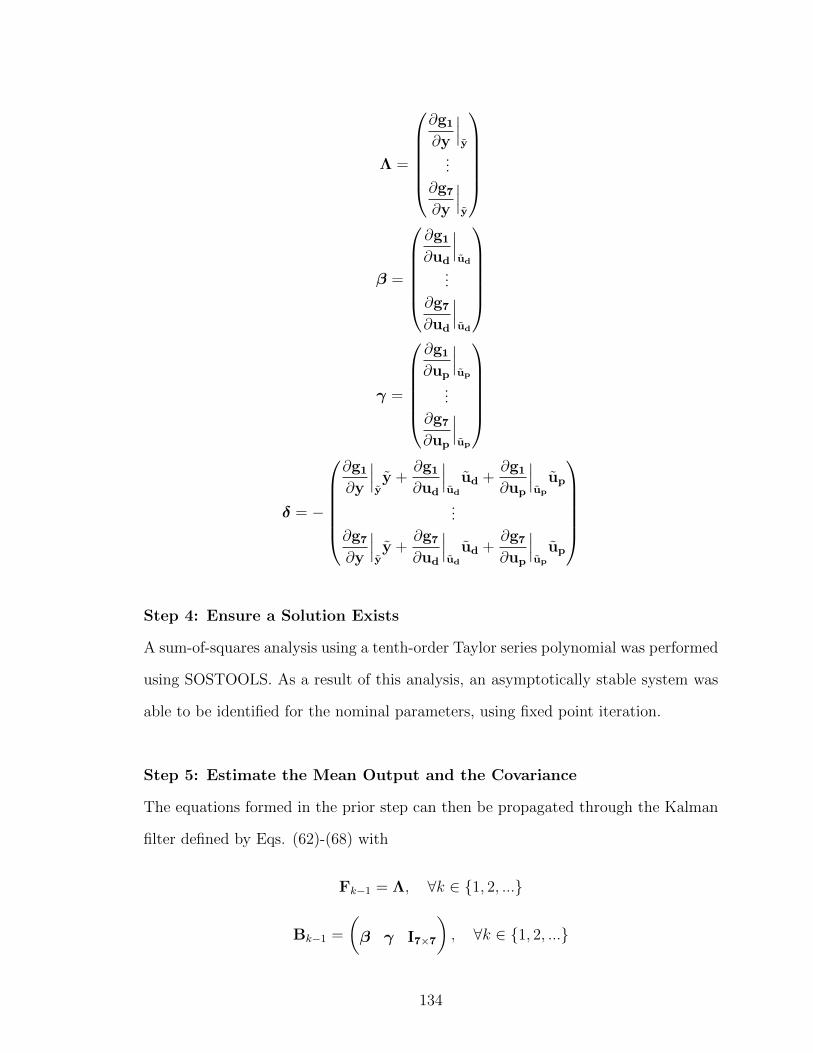
Λ =
∂g1
∂y
∣∣∣y
...
∂g7
∂y
∣∣∣y
β =
∂g1
∂ud
∣∣∣ud
...
∂g7
∂ud
∣∣∣ud
γ =
∂g1
∂up
∣∣∣up
...
∂g7
∂up
∣∣∣up
δ = −
∂g1
∂y
∣∣∣yy +
∂g1
∂ud
∣∣∣ud
ud +∂g1
∂up
∣∣∣up
up
...
∂g7
∂y
∣∣∣yy +
∂g7
∂ud
∣∣∣ud
ud +∂g7
∂up
∣∣∣up
up
Step 4: Ensure a Solution Exists
A sum-of-squares analysis using a tenth-order Taylor series polynomial was performed
using SOSTOOLS. As a result of this analysis, an asymptotically stable system was
able to be identified for the nominal parameters, using fixed point iteration.
Step 5: Estimate the Mean Output and the Covariance
The equations formed in the prior step can then be propagated through the Kalman
filter defined by Eqs. (62)-(68) with
Fk−1 = Λ, ∀k ∈ 1, 2, ...
Bk−1 =
(β γ I7×7
), ∀k ∈ 1, 2, ...
134
uk−1 =
ud
up
δ
, ∀k ∈ 1, 2, ...
where in this example ud = ud and up = 0. Since there are uncertainties with the
model, the matrix Q is not null and the appropriate elements are populated with the
model uncertainties. The unscented transform is used on an uncoupled system with
the distribution described in Step 2 (and Table 12) in order to identify y0 and Σ0, the
initial output mean and covariance for each design. A design is considered converged
when the absolute difference between iteration estimates is less than 1× 10⁻⁴ or the
relative difference is less than 1× 10⁻⁶.
Step 6: Identify the Mean and Variance Bound of the Objective Function
Upon convergence the mean values of mdeploy, sf , and dmiss (e.g., mdeploy, sf , and
dmiss) can be calculated using the output of the converged Kalman filter equations
from Step 5. The mass is an output of the weights and sizing CA while the mass
and miss distance are outputs from the trajectory CA. The estimate for the variance
(i.e., the variance bound) in this case is simply
σ2r ≤‖ Σy∗x ‖2
where x in y∗x is either the deployable mass, mdeploy, the range, sf , or the miss distance
dmiss.
Step 7: Optimize for Uncertainty and Ensure Constraints are Met
Formulating the output of Step 6 in terms of the mean and variance allows for an op-
timal control problem to be setup for the system design, where the objective function
135
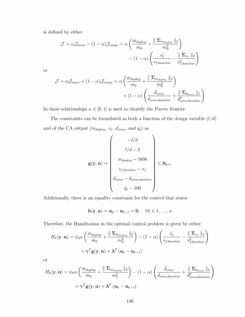
is defined by either
J = αJmass − (1− α)Jrange = α
(mdeploy
m0
+‖ Σmdeploy
‖2
m20
)− (1− α)
(sf
sf,baseline−‖ Σsf ‖2
s2f,baseline
)or
J = αJmass + (1− α)Jrange = α
(mdeploy
m0
+‖ Σmdeploy
‖2
m20
)+ (1− α)
(dmiss
dmiss,baseline+‖ Σdmiss
‖2
d2miss,baseline
)In these relationships α ∈ [0, 1] is used to identify the Pareto frontier.
The constraints can be formulated as both a function of the design variable (l/d)
and of the CA output (mdeploy, sf , dmiss, and qs) as
g(y,u) =
−l/d
l/d− 2
mdeploy − 5000
sf,baseline − sf
dmiss − dmiss,baseline
qs − 100
≤ 06×1
Additionally, there is an equality constraint for the control that states
h(y,u) = uk − uk−1 = 0, ∀k ∈ 1, . . . , n
Therefore, the Hamiltonian in the optimal control problem is given by either
Hk(y,u) = ψ0α
(mdeploy
m0
+‖ Σmdeploy
‖2
m20
)− (1− α)
(sf
sf,baseline−‖ Σsf ‖2
s2f,baseline
)
+ γTg(y,u) + λT (uk − uk−1)
or
Hk(y,u) = ψ0α
(mdeploy
m0
+‖ Σmdeploy
‖2
m20
)− (1− α)
(dmiss
dmiss,baseline+‖ Σdmiss
‖2
d2miss,baseline
)
+ γTg(y,u) + λT (uk − uk−1)
136
where the terms in these relations can be computed numerically. The discrete optimal
control conditions listed in Chapter 3 can then be used to compute the value of ud
for a chosen value of α.
5.6.6 Design Results
The results of the sizing of the deployable aerodynamic surface are presented in the
sections that follow.
5.6.6.1 Single-Delta Design Solutions
Converged, optimal deployable designs for the single-delta configuration are shown in
Figs. 40 and 41. The points denoted with circles correspond to optimal designs found
using the rapid robust multidisciplinary design methodology and points denoted with
an ‘x’ correspond to optimal designs found using a multi-objective particle swarm
optimizer (MOPSO) wrapped around a Monte Carlo simulation. The 1σ robustness
estimate provided by the Monte Carlo is the result of increasing the number of samples
until the change was less than 0.1%.
Correlation between the MOPSO results and those obtained through the rapid ro-
bust design methodology is seen in both Figs. 40 and 41. The discrepancy in values
can be attributed to the conservatism provided by the rapid robust design method-
ology with respect to the estimation of the variance as well as the inherent linearity
of the methodology. The variance bound approximates the variance in the response
of the design (i.e., the 1σ mass, range, or accuracy) with the largest eigenvalue of
the propagated covariance matrix, which is conservative and is seen throughout the
results. In addition, the sequential linearization procedure to accommodate nonlin-
earities introduces errors in the resulting solutions. These are discussed further in
Chapter 6. However, these shortcomings are within those accepted by the conceptual
design community and are compensated for by the additional speed of the method-
ology.
137

0 50 100 150 200 250 3004600
4800
5000
5200
5400
5600
5800
6000
6200
6400
6600
1σ Deployable Mass, kg
1σ R
ang
e, k
m
Rapid Robust Design MethodologyMOPSO around Monte Carlo
l/d = 0.01
l/d = 0.01
l/d = 1.14
l/d = 1.13
l/d = 1.99
l/d = 1.99
(a)
0 50 100 150 200 250 3004600
4800
5000
5200
5400
5600
5800
6000
6200
6400
6600
1σ Deployable Mass, kg
1σ R
ang
e, k
m
Rapid Robust Design MethodologyMOPSO around Monte Carlo
l/d = 1.16
l/d = 1.99
l/d = 0.01
l/d = 0.01
l/d = 1.16
l/d = 1.99
(b)
Figure 40: Design solutions for range comparing the rapid robust design methodol-ogy and a multiobjective particle swarm optimizer for a (a) bank-to-steer guidancealgorithm and the (b) acceleration control guidance algorithm.
138
0 50 100 150 200 250 3005
5.1
5.2
5.3
5.4
5.5
5.6
5.7
5.8
5.9
6
1σ Deployable Mass, kg
1σ A
ccu
racy
, km
Rapid Robust Design MethodologyMOPSO around Monte Carlo
l/d = 0.02
l/d = 1.35
l/d = 1.37
l/d = 1.99
l/d = 1.99
l/d = 0.01
(a)
0 50 100 150 200 250 3000
0.5
1
1.5
2
2.5
3
1σ Deployable Mass, kg
1σ A
ccu
racy
, km
Rapid Robust Design MethodologyMOPSO around Monte Carlo
l/d = 1.99
l/d = 1.99l/d = 1.14
l/d = 1.15
l/d = 0.01
l/d = 0.02
(b)
Figure 41: Design solutions for accuracy comparing the rapid robust design method-ology and a multiobjective particle swarm optimizer for a (a) bank-to-steer guidancealgorithm and the (b) acceleration control guidance algorithm.
139
Figure 40 demonstrates that the larger the deployable’s mass, the more range
capability the strategic system can achieve. In fact, for an approximately 300 kg
deployable, the range is improved over 1,200 km (an improvement of greater than
25%). The range is seen insensitive to the two guidance algorithms considered. This
is due to the fact that the trajectory for maximum range is largely a full-lift up
trajectory which is equally capable of being flown by a bank-to-steer algorithm and
the acceleration control method. For an equally weighted objective function between
range and mass, the optimal design has an l/d of 1.16 (mdeploy = 139 kg), regardless
of the guidance algorithm.
Figure 41 demonstrates that the larger the deployable is, the more accurate the
system will be. For an approximately 300 kg deployable, the accuracy is capable of
being improved by an order of magnitude from the baseline strategic system (from 2.8
km to 0.3 km). Unlike range, the accuracy of the system is sensitive to the guidance
algorithm. For the bank-to-steer algorithm, the control is nearly saturated with a
miss distance of about 5.5 km across all deployable sizes. However, using acceleration
control, improvement is consistently seen with a larger deployables (with larger L/D).
For an equally weighted objective function between range and mass using acceleration
control, the optimal design has a l/d of 1.14 (mdeploy = 131 kg).
A significant advantage of the rapid robust design methodology is computational
runtime. This is shown in Table 13 where the number of iterations required to obtain
the results shown in Figs. 40 and 41 is provided.
Despite returning approximately four times as many optimal solutions as the
MOPSO approach, the number of analysis iterations of the rapid robust design
methodology is an order of magnitude less (with runtimes less than 5%) than the
MOPSO. In addition, the probabilistic results obtained by this new methodology are
within 10% of those obtained using the MOPSO, with the vast majority having errors
less than 3% the MOPSO values.
140
Table 13: Computational comparison between MOPSO and the Rapid Robust DesignMethodology.
Range AccuracyRapid Robust Rapid Robust
Design DesignMethodology MOPSO Methodology MOPSO
Number of24,962 710,108 28,616 841,094
DSM Iterations, -Computational
2.2 69.7 2.4 85.7Runtime, hours
Center of Gravity Considerations
The results presented thus far allow for the center of gravity (CG) to be positioned
anywhere, including outside the outer mold line of the vehicle. This is not practical.
As shown in Fig. 42, when limiting the CG to be within the vehicle, as l/d increases,
the maximum L/D achievable diminishes to a point where it is actually less than the
baseline system.
In order to achieve trim conditions with practical values of CG position, a body
flap was added to the baseline system. This body flap was assumed to be a flat surface
that was 25% of the vehicle’s length. Figure 43 shows that the body flap deflection
angle in order to achieve maximum L/D. Note that the deflection angle remains less
than 30 for all deployable sizes considered.
141

0 0.5 1 1.5 2
0.7
0.8
0.9
1
1.1
1.2
1.3
1.4
l/d, −
(L/D
)/(L
/D) ba
selin
e, −
CG Not Considered
CG in Body
(a)
0 0.5 1 1.5 21
1.2
1.4
1.6
1.8
2
2.2
2.4
l/d, −
Dia
met
ers
Out
side
of B
ody
to T
rim a
t (L/
D) m
ax, −
(b)
Figure 42: The (a) impact on L/D of constraining the CG position to be within thevehicle and (b) the normalized (relative to the vehicle’s diameter) distance outsidethe vehicle the CG needs to be to achieve (L/D)max.
142
0 0.5 1 1.5 20
5
10
15
20
25
30
l/d, −
Bod
y F
lap
Def
lect
ion
Ang
le, °
Figure 43: Body flap deflection angle required to trim the vehicle at the theoreticalmaximum L/D.
5.6.6.2 Alternative Configuration
An additional deployable configurations were assessed to identify whether an improve-
ment in L/D can be obtained without the inclusion of a body flap. This configuration
is shown in Fig. 44.
(L/D)max = 1.02
(L/D)max,trim = 1.00
Baseline
(L/D)max 1.24
(L/D)max,trim 1.01
(L/D)max,trim/(L/D)max,trim|baseline = 1.01
(L/D)max 1.53
(L/D)max,trim 1.52
(L/D)max,trim/ /(L/D)max,trim|baseline = 1.52
Single-Delta Double-Delta
Figure 44: Comparison of investigated deployable concepts showing the maximumachievable L/D accounting for trim considerations.
While the single-delta deployable concept previously described does not provide
143
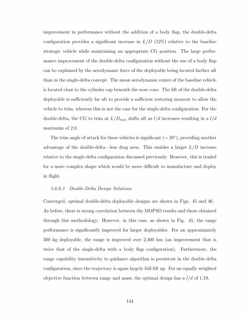
improvement in performance without the addition of a body flap, the double-delta
configuration provides a significant increase in L/D (52%) relative to the baseline
strategic vehicle while maintaining an appropriate CG position. The large perfor-
mance improvement of the double-delta configuration without the use of a body flap
can be explained by the aerodynamic force of the deployable being located farther aft
than in the single-delta concept. The mean aerodynamic center of the baseline vehicle
is located close to the cylinder cap beneath the nose cone. The lift of the double-delta
deployable is sufficiently far aft to provide a sufficient restoring moment to allow the
vehicle to trim, whereas this is not the case for the single-delta configuration. For the
double-delta, the CG to trim at L/Dmax shifts aft as l/d increases resulting in a l/d
maximum of 2.0.
The trim angle of attack for these vehicles is significant (∼ 20), providing another
advantage of the double-delta—less drag area. This enables a larger L/D increase
relative to the single-delta configuration discussed previously. However, this is traded
for a more complex shape which would be more difficult to manufacture and deploy
in flight.
5.6.6.3 Double-Delta Design Solutions
Converged, optimal double-delta deployable designs are shown in Figs. 45 and 46.
As before, there is strong correlation between the MOPSO results and those obtained
through this methodology. However, in this case, as shown in Fig. 45, the range
performance is significantly improved for larger deployables. For an approximately
300 kg deployable, the range is improved over 2,400 km (an improvement that is
twice that of the single-delta with a body flap configuration). Furthermore, the
range capability insensitivity to guidance algorithm is persistent in the double-delta
configuration, since the trajectory is again largely full-lift up. For an equally weighted
objective function between range and mass, the optimal design has a l/d of 1.19,
144
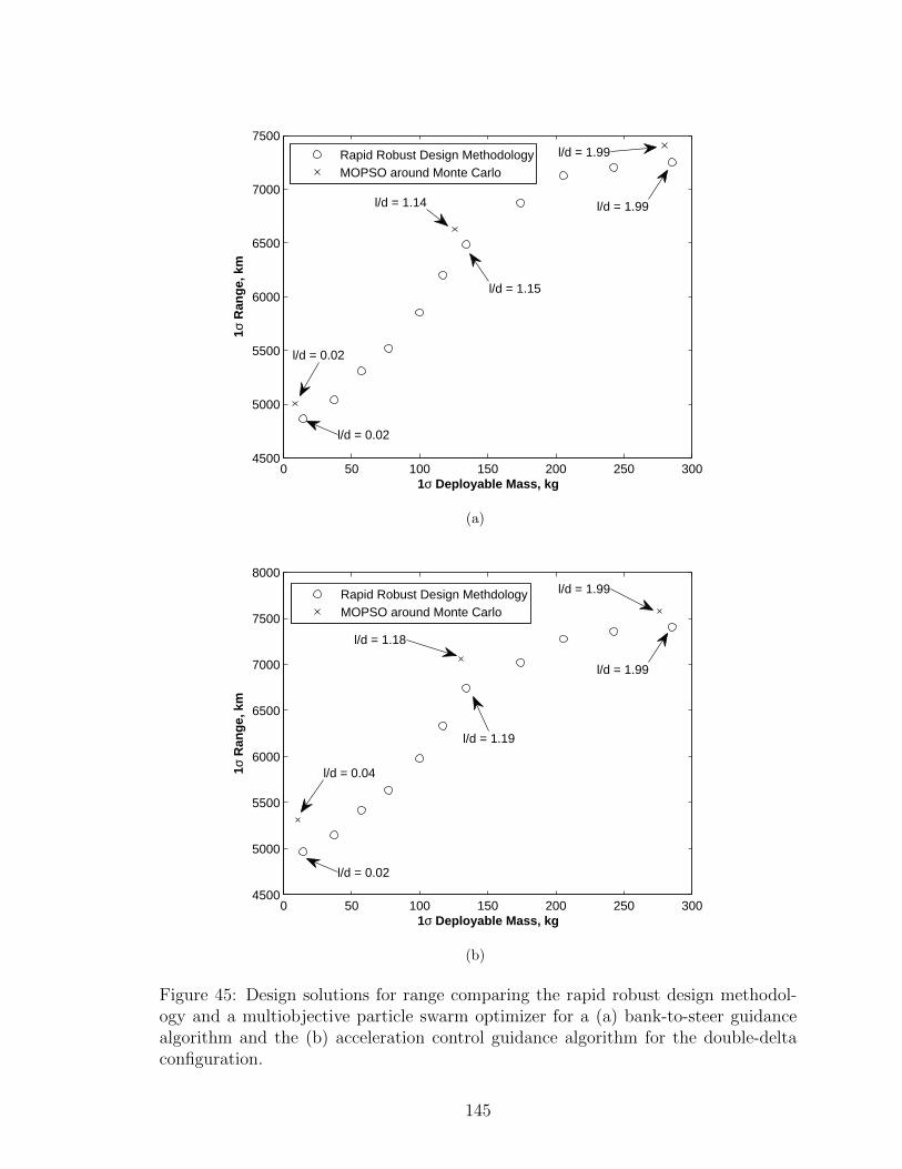
0 50 100 150 200 250 3004500
5000
5500
6000
6500
7000
7500
1σ Deployable Mass, kg
1σ R
ang
e, k
m
Rapid Robust Design MethodologyMOPSO around Monte Carlo
l/d = 0.02
l/d = 1.14
l/d = 1.99
l/d = 0.02
l/d = 1.15
l/d = 1.99
(a)
0 50 100 150 200 250 3004500
5000
5500
6000
6500
7000
7500
8000
1σ Deployable Mass, kg
1σ R
ang
e, k
m
Rapid Robust Design MethdologyMOPSO around Monte Carlo
l/d = 0.04
l/d = 1.18
l/d = 1.99
l/d = 0.02
l/d = 1.19
l/d = 1.99
(b)
Figure 45: Design solutions for range comparing the rapid robust design methodol-ogy and a multiobjective particle swarm optimizer for a (a) bank-to-steer guidancealgorithm and the (b) acceleration control guidance algorithm for the double-deltaconfiguration.
145
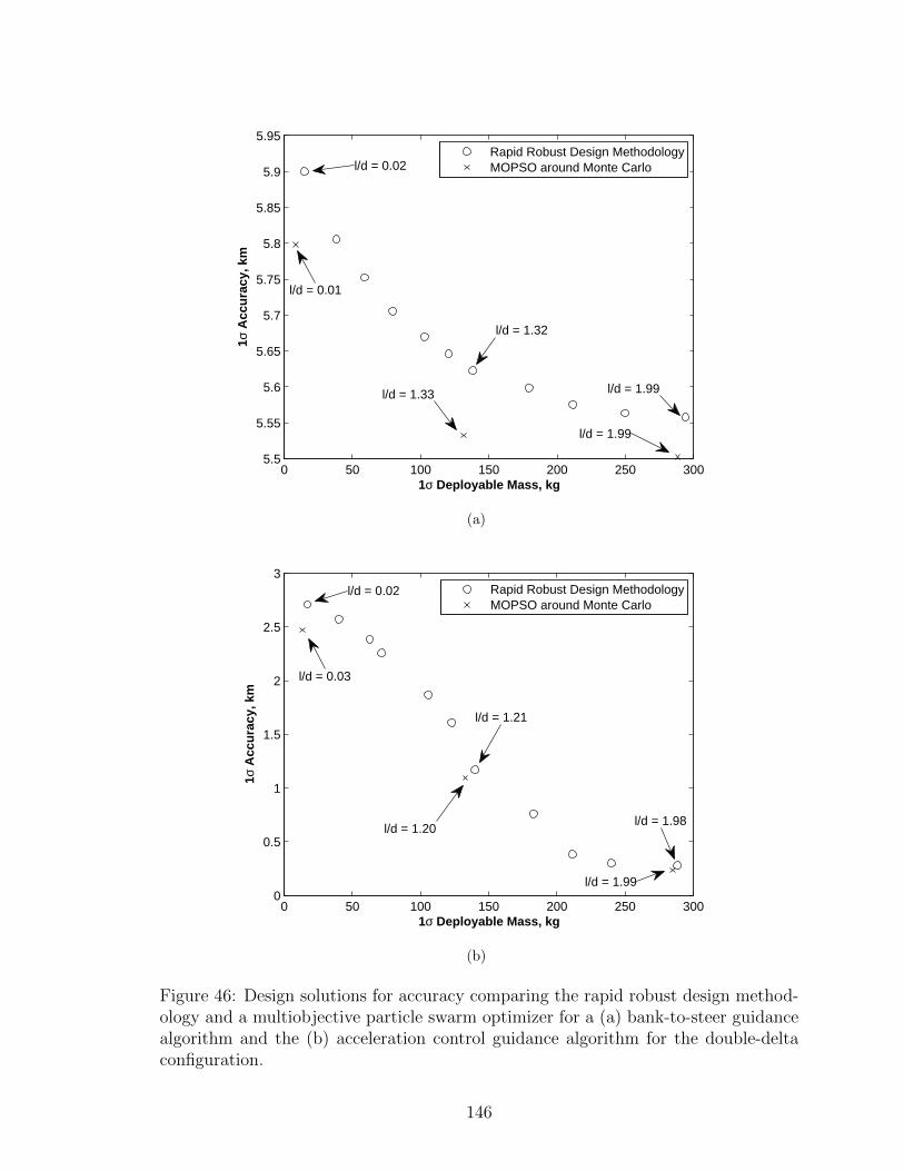
0 50 100 150 200 250 3005.5
5.55
5.6
5.65
5.7
5.75
5.8
5.85
5.9
5.95
1σ Deployable Mass, kg
1σ A
ccu
racy
, km
Rapid Robust Design MethodologyMOPSO around Monte Carlo
l/d = 0.01
l/d = 1.33
l/d = 1.99
l/d = 0.02
l/d = 1.32
l/d = 1.99
(a)
0 50 100 150 200 250 3000
0.5
1
1.5
2
2.5
3
1σ Deployable Mass, kg
1σ A
ccu
racy
, km
Rapid Robust Design MethodologyMOPSO around Monte Carlo
l/d = 0.02
l/d = 0.03
l/d = 1.20
l/d = 1.21
l/d = 1.99
l/d = 1.98
(b)
Figure 46: Design solutions for accuracy comparing the rapid robust design method-ology and a multiobjective particle swarm optimizer for a (a) bank-to-steer guidancealgorithm and the (b) acceleration control guidance algorithm for the double-deltaconfiguration.
146
regardless of the guidance algorithm (mdeploy = 148 kg).
Figure 46 shows trends for the double-delta that are similar to those observed for
the single-delta configuration—the larger the deployable is, the more accurate the
system. When considering accuracy, however, the performance gain of the double-
delta configuration is not as great compared to range benefits. For an approximately
300 kg deployable, the 1σ accuracy is 0.2 km for the double-delta configuration,
compared to 0.3 km for the single-delta. However, the double-delta configuration is
characterized by a faster rate of improving accuracy as the deployable increases in
size (from an l/d of 0 to l/d of 2.0) compared to the single-delta and a body flap is not
required in order to achieve these performance gains. Again, 1σ accuracy of the system
is sensitive to the guidance algorithm, with the bank-to-steer guidance demonstrating
saturated qualities. For an equally weighted objective function between range and
mass using acceleration control, the optimal design has a l/d of 1.2 (mdeploy = 149
kg).
The computational runtime advantage (factor of 30) of the rapid robust design
methodology is shown in Table 14 where accuracies acceptable to conceptual design
are shown to be achievable.
Table 14: Computational comparison between MOPSO and the Rapid Robust DesignMethodology.
Range AccuracyRapid Robust Rapid Robust
Design DesignMethodology MOPSO Methodology MOPSO
Number of26,842 642,132 33,534 713,124
DSM Iterations, -Computational
2.3 59.6 2.8 64.2Runtime, hours
147
5.6.7 Conclusions
The rapid robust design methodology was implemented to optimize the design of a
deployable system for a strategic system. This methodology was shown to provide
similar results to traditional Monte Carlo methods with solutions within 10% for less
than 5% of the computational time.
Two deployable configurations were investigated—a single-delta and a double-
delta. For a 300 kg deployable, the single-delta configuration was shown to provide
an increase in 1σ range of more than 1,200 km (25%) and a reduction in 1σ miss
distance from 2.5 km to 0.5 km (500%) over the baseline strategic system. For this
configuration, a body flap is required for physical realizable CG positions. A 300
kg double-delta is able to increase the baseline system’s 1σ range by over 2,400 km
(50%) and reduce the 1σ miss distance by an order of magnitude (to less than 0.25
km) without the use of a body flap.
In addition to configuration, the effect of guidance algorithm was investigated
using a bank-to-steer algorithm and a bounding guidance algorithm. The range re-
sults were insensitive to guidance algorithm selection. However, when accuracy is
considered, guidance algorithm selection was shown to have a large effect as the
bank-to-steer algorithm’s control was shown to be nearly saturated with marginal
performance gains across the deployable sizes investigated.
5.7 Summary
This chapter demonstrated the use of dynamical system theory in multidisciplinary
design through several applications of increasing complexity. A probabilistic perfor-
mance assessment of the robustness methodology as well as example robust design
problems were provided, demonstrating application of dynamical system theory to
multidisciplinary design. The probabilistic assessment showed that the robustness
assessment methodology had maximum errors relative to exact values less than 1%
148
on the mean objective value and less than approximately 35% in standard deviation
for a large design space. In addition, for specific values of the CAs, a comparison
between traditional uncertainty quantification techniques and the rapid robustness
assessment methodology demonstrated significant computational advantages of the
developed methodology. The capability of stability theory to provide ranges of initial
values to start the iteration was demonstrated along with the capability to compute
the rate at which the design will converge. Through the design examples, application
to nonlinear and practical problems were demonstrated. For the two-bar truss, the
successive linearization procedure showed a minimal mass design that is consistent
with that found in the literature while rapidly characterizing both optimal and ro-
bust designs. The computational advantages of the technique was also demonstrated
in robust design of a deployable aerodynamic surface for a strategic system. Fam-
ilies of comparable designs for this large, highly nonlinear problem were found 25
times faster than using Monte Carlo methods coupled with traditional multiobjective
optimization techniques.
149
CHAPTER VI
COMPUTATIONAL PERFORMANCE OF THE RAPID
ROBUST DESIGN METHODOLOGY
This chapter describes the range of applicability for the rapid robust design methodol-
ogy from a computational perspective. This includes an analysis of the computational
cost associated with design complexity. The accuracy of the linear rapid robust de-
sign methodology is considered for general problems using nonlinear perturbation
analysis, providing a basis to identify the region in which the successive linearization
procedure is valid. A discussion of the conservatism resulting from use of the matrix
two-norm as a bound on design variance is also provided.
6.1 Computational Effect of Increasing the Design Com-plexity on the Rapid Robust Design Methodology
The previous chapter demonstrated the use of the rapid robust design methodology on
several example applications ranging from analytical problems to a problem relevant
to the EDL community. For these problems, the number of function evaluations
were reduced by a factor that approached thirty relative to traditional Monte Carlo
methods wrapped in an evolutionary optimizer. The following sections examine the
effect of design complexity on the number of function evaluations required to obtain
a solution. Quantitatively defining the complexity of the design is a matter of debate
amongst experts[199, 200, 201, 202]. In this investigation, the following definition will
be employed.
Definition: Design Complexity
Design complexity is the relative difficulty in obtaining an optimal design.
150
In the sections that follow, design complexity is used in the structural sense[201]. In
terms of the MDO problem, structural design complexity is comprised of components
such as the number of design variables, the number of CAs, the nonlinearity of the
CAs, and the nonlinearity of the response function. For the rapid robust design
methodology developed in this work, the effect of each of these components are first
examined individually, then several overall evaluation criterion are applied. Some of
these overall evaluation criterion also evaluate the strength of coupling between the
CAs.
6.1.1 Test Problem Definition
To assess the effect of increasing design complexity on the computational efficiency
of the rapid robust design methodology, a generalized test problem was formulated.
This test problem is shown in Fig. 47.
The DSM in Fig. 47 is fully coupled and can be functionally represented as
yi = f(y1,y2, · · · ,yi−1,yi+1, · · · ,yn−1,yn,u) (114)
where in this case f(·) and each CA are scalar functions. The function in Eq. (114)
is represented as an qth-order polynomial
f(y1,y2, · · · ,yi−1,yi+1, · · · ,yn−1,yn,u) =
q∑j1=1
q∑j2=1
· · ·q∑
jn−1=1
q∑jn=1
[a(j1, j2, · · · jn−1, jn)yj11 y
j22 · · · y
jn−1
n−1 yjnn +
d+p∑i=1
ui
](115)
Similarly, the response function is a rth-order polynomial consisting of the outputs
for each of the contributing analysis
r =r∑
j1=1
r∑j2=1
· · ·r∑
jn−1=1
r∑jn=1
b(j1, j2, · · · jn−1, jn)yj11 yj22 · · · y
jn−1
n−1 yjnn (116)
In each case the coefficients, are given by
a(j1, j2, · · · jn−1, jn) =
U(−1, 1), ji 6= i
0, ji = i(117)
151

Co
ntr
ibu
tin
g A
nal
ysis
1
Co
ntr
ibu
tin
g A
nal
ysis
2
Co
ntr
ibu
tin
g A
nal
ysis
n-2
Co
ntr
ibu
tin
g A
nal
ysis
n-1
Co
ntr
ibu
tin
g A
nal
ysis
n
Co
ntr
ibu
tin
g A
nal
ysis
3
Fig
ure
47:
Gen
eral
des
ign
stru
cture
mat
rix
for
anal
yzi
ng
the
effec
tof
des
ign
com
ple
xit
y.
152
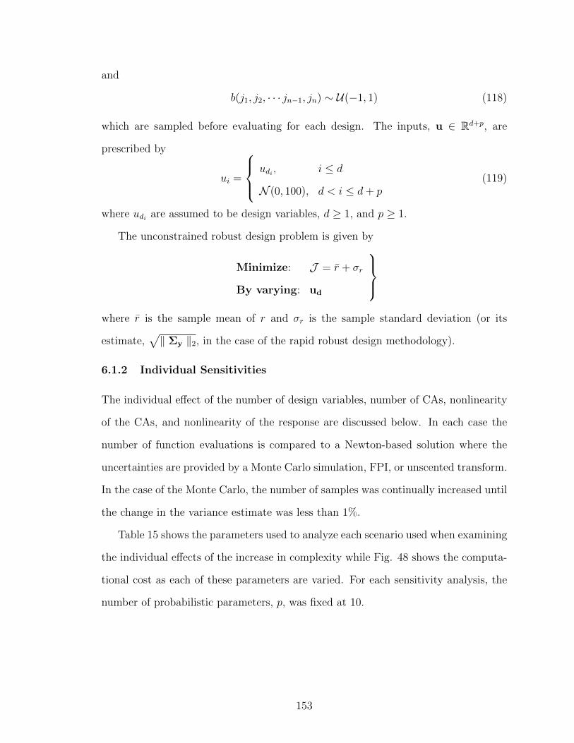
and
b(j1, j2, · · · jn−1, jn) ∼ U(−1, 1) (118)
which are sampled before evaluating for each design. The inputs, u ∈ Rd+p, are
prescribed by
ui =
udi , i ≤ d
N (0, 100), d < i ≤ d+ p(119)
where udi are assumed to be design variables, d ≥ 1, and p ≥ 1.
The unconstrained robust design problem is given by
Minimize: J = r + σr
By varying: ud
where r is the sample mean of r and σr is the sample standard deviation (or its
estimate,√‖ Σy ‖2, in the case of the rapid robust design methodology).
6.1.2 Individual Sensitivities
The individual effect of the number of design variables, number of CAs, nonlinearity
of the CAs, and nonlinearity of the response are discussed below. In each case the
number of function evaluations is compared to a Newton-based solution where the
uncertainties are provided by a Monte Carlo simulation, FPI, or unscented transform.
In the case of the Monte Carlo, the number of samples was continually increased until
the change in the variance estimate was less than 1%.
Table 15 shows the parameters used to analyze each scenario used when examining
the individual effects of the increase in complexity while Fig. 48 shows the computa-
tional cost as each of these parameters are varied. For each sensitivity analysis, the
number of probabilistic parameters, p, was fixed at 10.
153
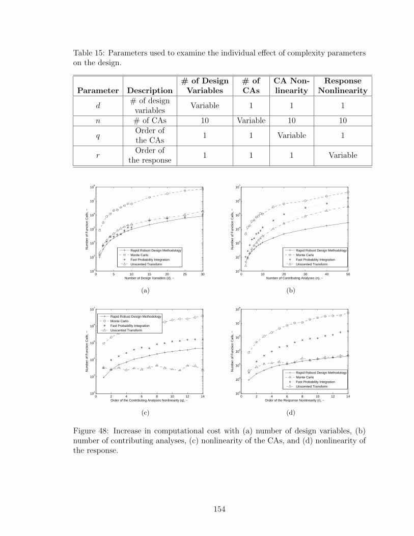
Table 15: Parameters used to examine the individual effect of complexity parameterson the design.
# of Design # of CA Non- ResponseParameter Description Variables CAs linearity Nonlinearity
d# of design
Variable 1 1 1variables
n # of CAs 10 Variable 10 10
qOrder of
1 1 Variable 1the CAs
rOrder of
1 1 1 Variablethe response
0 5 10 15 20 25 3010
2
103
104
105
106
107
108
Number of Design Variables (d), −
Num
ber
of F
unct
ion
Cal
ls, −
Rapid Robust Design MethodologyMonte CarloFast Probability IntegrationUnscented Transform
(a)
0 10 20 30 40 5010
1
102
103
104
105
106
107
Number of Contributing Analyses (n), −
Num
ber
of F
unct
ion
Cal
ls, −
Rapid Robust Design MethodologyMonte CarloFast Probability IntegrationUnscented Transform
(b)
0 2 4 6 8 10 12 1410
2
103
104
105
106
107
Order of the Contributing Analyses Nonlinearity (q), −
Num
ber
of F
unct
ion
Cal
ls, −
Rapid Robust Design MethodologyMonte CarloFast Probability IntegrationUnscented Transform
(c)
0 2 4 6 8 10 12 1410
2
103
104
105
106
107
108
Order of the Response Nonlinearity (r), −
Num
ber
of F
unct
ion
Cal
ls, −
Rapid Robust Design MethodologyMonte CarloFast Probability IntegrationUnscented Transform
(d)
Figure 48: Increase in computational cost with (a) number of design variables, (b)number of contributing analyses, (c) nonlinearity of the CAs, and (d) nonlinearity ofthe response.
154

6.1.2.1 Effect of Number of Design Variables
In this case, the number of design variables, d, is varied while the other parameters
were held constant as shown in Table 15. Figure 48(a) shows that each of the methods
exhibit algebraic growth with number of design variables (i.e., the number of function
calls goes as O(nc) for some c). As a Newton optimization algorithm is being utilized,
this is expected. It is also observed that the Monte Carlo solutions have an order of
magnitude more function evaluations compared to the other techniques considered.
This is expected since the rapid robust design methodology, FPI, and unscented
transform require a fixed number of function evaluations to obtain the mean and the
variance.
6.1.2.2 Effect of Number of Contributing Analyses
The number of CAs is representative of the complexity of the problem domain. To
analyze this effect on the number of function calls, the number of CAs, n, is varied
while the other parameters were held constant as shown in Table 15. As seen in
Fig. 48(b), each of the methods exhibit approximately algebraic growth with the
number of CAs. The increase in the number of function calls is a result of the fixed-
point iteration requiring an increasing number of iterations in order to reach the
convergence tolerance. For larger designs (greater than 20 CAs), the rate of function
call growth with number of CAs is similar between each of the methods. However,
for small designs (less than 20 CAs) the rapid robust design methodology is observed
to have the slowest rate of growth.
6.1.2.3 Effect of Contributing Analysis Nonlinearity
The effect of CA nonlinearity was assessed by varying the maximum degree of the
polynomial defined in Eq. (115), q. Each of the ten CAs’ order is varied simultane-
ously so that each polynomial has the same number of terms. The other parameters
used in this analysis are shown in Table 15. Figure 48(c) shows that the rapid robust
155
design methodology and FPI again exhibit algebraic growth with the number of CAs
due to the fact that they rely on successive linearization to approximate the sys-
tem. Since the unscented transform does not depend on the linearity of the CAs and
propagates the same number of samples based on the dimensionality of the problem
(n + d + p), it has no sensitivity to the nonlinearity of the CAs. The Monte Carlo
exhibits algebraic growth initially, with exponential growth (i.e., number of functions
calls ∼ O(cq)) for highly nonlinear systems. This can be attributed to the fact that
the Monte Carlo simulation ensures that the change in the variance estimate is less
than 1%, requiring additional sampling for more nonlinear designs.
6.1.2.4 Effect of Response Nonlinearity
The effect of response nonlinearity was assessed by varying the maximum degree of the
polynomial defined in Eq. (116), r. The parameters used in this analysis are shown
in Table 15 while the variation in the number of function calls required to obtain a
robust design is shown in Fig. 48(d). The variation in the number of function calls
required by the rapid robust design methodology and unscented transform as the
response nonlinearity is increased is similar. Both of the techniques exhibit quasi-
linear growth behavior for increasing nonlinearity, while the Monte Carlo and FPI
exhibit an algebraic increase in the number of function calls.
6.1.3 Overall Complexity Metrics
An overall complexity index could also be used to measure the performance of the
rapid robust design methodology compared to traditional methods. Four different
metrics are considered—an algebraic metric, a Jacobian metric, a force-based clus-
tering metric, and an input-output graphical based metric. In addition providing
information about the structure of the design problem, the Jacobian and the force
based clustering metric also account for the functional relationship within the design.
That is to say, in addition to topological considerations in the design, these metrics
156

account for how strongly coupled the design is or what the mapping between the
input and output looks like.
6.1.3.1 Algebraic Metric
The algebraic metric combines the four individual metrics discussed previously—the
number of design variables, the number of CAs, the nonlinearity of the CAs, and the
order of the response. The metric considered is defined as follows
Ca = dr
(n∑i=1
qi
)(120)
where qi is the order of the ith CA. In this metric, the size and the order of the CAs
are combined into a single value, the summation of the order of each CA; however,
for a linear design, this reduces to the number of CAs.
6.1.3.2 Jacobian Metric
The Jacobian metric augments the algebraic metric with the addition of the order
of the matrix of partial derivatives between the input and output of the design.
Specifically, this metric is defined as
CJ = Cad∑i=1
O(∂r
∂ud
)i
= dr
(n∑i=1
qi
)(d∑i=1
O(∂r
∂ud
)i
)(121)
The Jacobian captures the sensitivity of the output to perturbations in the input and
is used in many optimization algorithms (e.g., steepest-descent).
6.1.3.3 Force-Based Clustering Metric
Force-based clustering is a graphical method that can be used to reorder a design
into a structured DSM and simultaneously provides information on the strength of
the connection between CAs[30]. This method works by modeling the connections
between CAs with an attractive force that clusters CAs with strong linkages, pulling
CAs that use the same information together. Decomposing the problem in this way
arranges the DSM in the “lowest energy” state, which can be used to measure the
157
strength of the connections between the CAs. This complexity index augments the
algebraic metric with the summation of these forces once the DSM is arranged in the
minimal energy state.
Cfbc = CaJfbc = drJfbc
(n∑i=1
qi
)(122)
where Jfbc is the sum of the edges of the force-based clustering graph when decom-
posed.
6.1.3.4 Input-Output Graph Metric
The last metric considered is a graphical technique based on the topology of the
design. In this method the net information flow through each CA is considered. That
is the difference between the number of output variables to the number of used input
variables is utilized,
Cio = Can∑i=1
(dim(yi,out)− dim(yi,in))
= dr
(n∑i=1
qi
)(n∑i=1
(dim(yi,out)− dim(yi,in))
) (123)
where yi,out and yi,in are the number of output variables and used input variables,
respectively.
6.1.3.5 Correlation Between Computational Cost and Complexity
The use of each of these techniques is demonstrated in Fig. 49 for nine representative
designs. These designs varied from a linear, weakly coupled three CA system with
a single input to a nonlinear design with 20 CAs, five design variables, and a highly
nonlinear response. Each design case is shown in Table 16 where the number of
probabilistic parameters, p, is assumed to be 5 for each case.
From Fig. 49, it is observed that the number of function calls generally increase for
each metric. However, the number of function calls does not monotonically increase
with the Jacobian augmented metric. Furthermore, as seen by the same complexity
158

Table 16: Design cases used to evaluate the overall complexity metrics.
Case Case Case Case Case Case Case Case CaseParameter 1 2 3 4 5 6 7 8 9
n 3 3 3 3 3 10 10 20 20q 1 2 1 5 5 1 5 1 5r 1 1 2 1 5 1 5 1 5d 1 1 1 5 5 1 5 1 5
100
101
102
103
104
102
103
104
105
106
107
108
Algebraic Complexity Metric, −
Num
ber
of F
unct
ion
Cal
ls, −
Rapid Robust Design MethodologyMonte CarloFast Probability IntegrationUnscented Transform
(a)
100
101
102
103
104
102
103
104
105
106
107
108
Jacobian Complexity Metric, −
Num
ber
of F
unct
ion
Cal
ls, −
Rapid Robust Design MethodologyMonte CarloFast Probability IntegrationUnscented Transform
(b)
101
102
103
104
105
102
103
104
105
106
107
108
Force−Based Clustering Complexity Metric, −
Num
ber
of F
unct
ion
Cal
ls, −
Rapid Robust Design MethodologyMonte CarloFast Probability IntegrationUnscented Transform
(c)
100
101
102
103
104
102
103
104
105
106
107
108
Input−Output Complexity Metric, −
Num
ber
of F
unct
ion
Cal
ls, −
Rapid Robust Design MethodologyMonte CarloFast Probability IntegrationUnscented Transform
(d)
Figure 49: Increase in computational cost with complexities using the (a) algebraiccomplexity metric, (b) Jacobian complexity metric, (c) force-based clustering metric,and (d) input-output metric.
value resulting in multiple number of function calls, all metrics except force-based
clustering provided multiple values for the number of function calls for low complex-
ity designs. This makes the force-based clustering metric the most promising for
159
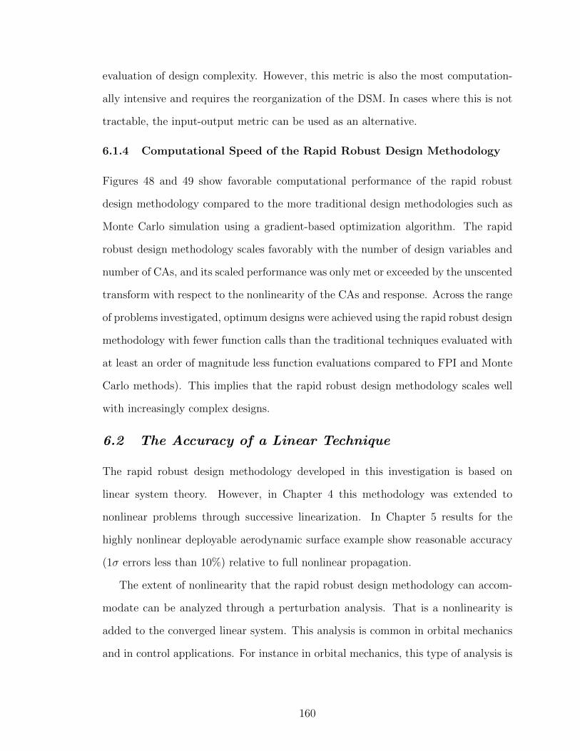
evaluation of design complexity. However, this metric is also the most computation-
ally intensive and requires the reorganization of the DSM. In cases where this is not
tractable, the input-output metric can be used as an alternative.
6.1.4 Computational Speed of the Rapid Robust Design Methodology
Figures 48 and 49 show favorable computational performance of the rapid robust
design methodology compared to the more traditional design methodologies such as
Monte Carlo simulation using a gradient-based optimization algorithm. The rapid
robust design methodology scales favorably with the number of design variables and
number of CAs, and its scaled performance was only met or exceeded by the unscented
transform with respect to the nonlinearity of the CAs and response. Across the range
of problems investigated, optimum designs were achieved using the rapid robust design
methodology with fewer function calls than the traditional techniques evaluated with
at least an order of magnitude less function evaluations compared to FPI and Monte
Carlo methods). This implies that the rapid robust design methodology scales well
with increasingly complex designs.
6.2 The Accuracy of a Linear Technique
The rapid robust design methodology developed in this investigation is based on
linear system theory. However, in Chapter 4 this methodology was extended to
nonlinear problems through successive linearization. In Chapter 5 results for the
highly nonlinear deployable aerodynamic surface example show reasonable accuracy
(1σ errors less than 10%) relative to full nonlinear propagation.
The extent of nonlinearity that the rapid robust design methodology can accom-
modate can be analyzed through a perturbation analysis. That is a nonlinearity is
added to the converged linear system. This analysis is common in orbital mechanics
and in control applications. For instance in orbital mechanics, this type of analysis is
160
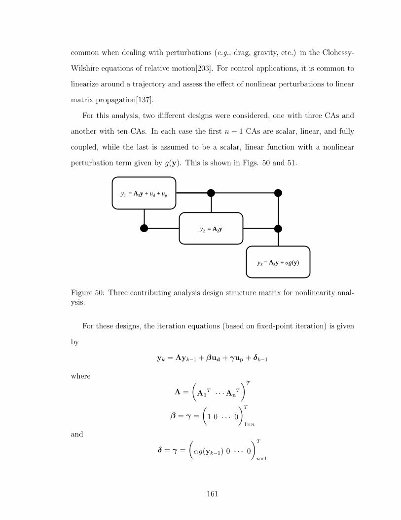
common when dealing with perturbations (e.g., drag, gravity, etc.) in the Clohessy-
Wilshire equations of relative motion[203]. For control applications, it is common to
linearize around a trajectory and assess the effect of nonlinear perturbations to linear
matrix propagation[137].
For this analysis, two different designs were considered, one with three CAs and
another with ten CAs. In each case the first n − 1 CAs are scalar, linear, and fully
coupled, while the last is assumed to be a scalar, linear function with a nonlinear
perturbation term given by g(y). This is shown in Figs. 50 and 51.
y1 = A1y + ud + up
y2 = A2y
y3 = A3y + αg(y)
Figure 50: Three contributing analysis design structure matrix for nonlinearity anal-ysis.
For these designs, the iteration equations (based on fixed-point iteration) is given
by
yk = Λyk−1 + βud + γup + δk−1
where
Λ =
(A1
T · · ·AnT
)Tβ = γ =
(1 0 · · · 0
)T1×n
and
δ = γ =
(αg(yk−1) 0 · · · 0
)Tn×1
161
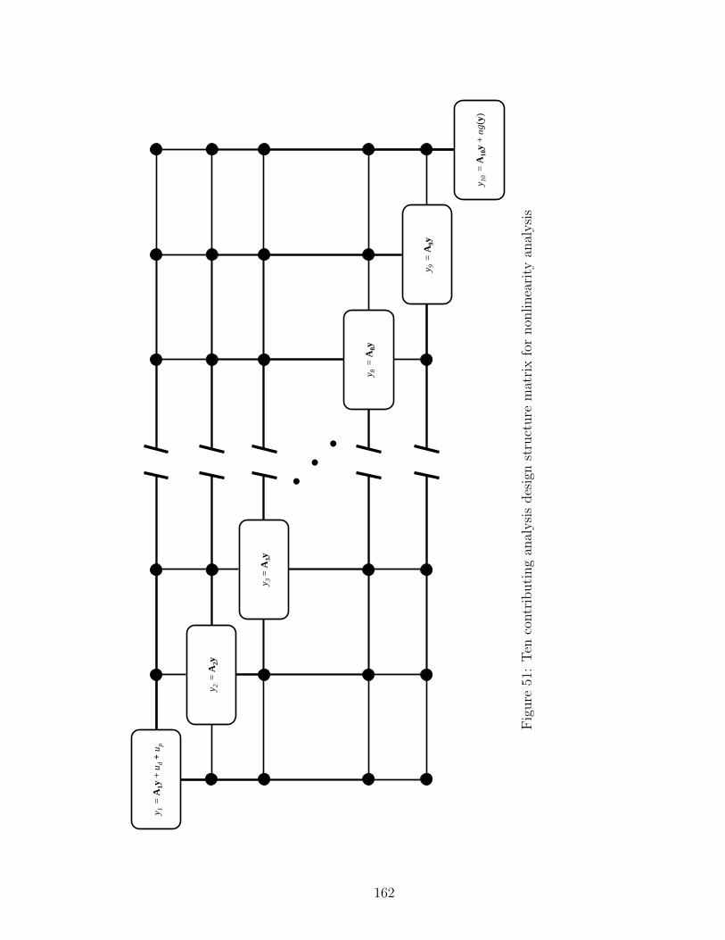
y 1 =
A1y
+ u
d +
up
y 2 =
A2y
y 8 =
A8y
y 9 =
A9y
y 10
= A
10y
+ α
g(y
)
y 3 =
A3y
Fig
ure
51:
Ten
contr
ibuti
ng
anal
ysi
sdes
ign
stru
cture
mat
rix
for
non
linea
rity
anal
ysi
s
162
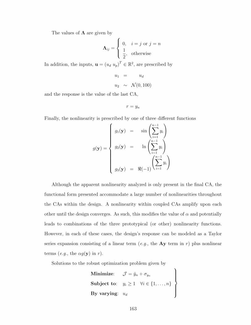
The values of Λ are given by
Λij =
0, i = j or j = n
1
2, otherwise
In addition, the inputs, u = (ud up)T ∈ R2, are prescribed by
u1 = ud
u2 ∼ N (0, 100)
and the response is the value of the last CA,
r = yn
Finally, the nonlinearity is prescribed by one of three different functions
g(y) =
g1(y) = sin
(n−1∑i=1
yi
)
g2(y) = ln
(n−1∑i=1
yi
)
g3(y) = <(−1)
(n−1∑i=1
yi
)
Although the apparent nonlinearity analyzed is only present in the final CA, the
functional form presented accommodate a large number of nonlinearities throughout
the CAs within the design. A nonlinearity within coupled CAs amplify upon each
other until the design converges. As such, this modifies the value of α and potentially
leads to combinations of the three prototypical (or other) nonlinearity functions.
However, in each of these cases, the design’s response can be modeled as a Taylor
series expansion consisting of a linear term (e.g., the Ay term in r) plus nonlinear
terms (e.g., the αg(y) in r).
Solutions to the robust optimization problem given by
Minimize: J = yn + σyn
Subject to: yi ≥ 1 ∀i ∈ 1, . . . , n
By varying: ud
163
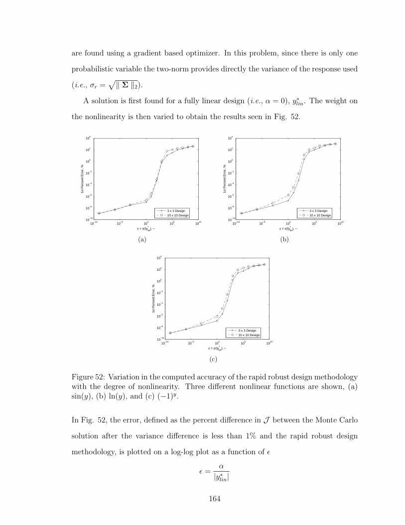
are found using a gradient based optimizer. In this problem, since there is only one
probabilistic variable the two-norm provides directly the variance of the response used
(i.e., σr =√‖ Σ ‖2).
A solution is first found for a fully linear design (i.e., α = 0), y∗lin. The weight on
the nonlinearity is then varied to obtain the results seen in Fig. 52.
10−10
10−5
100
105
1010
10−10
10−8
10−6
10−4
10−2
100
102
104
ε = α/|y*lin
|, −
1σ P
erce
nt E
rror
, %
3 x 3 Design10 x 10 Design
(a)
10−10
10−5
100
105
1010
10−10
10−8
10−6
10−4
10−2
100
102
104
ε = α/|y*lin
|, −1σ
Per
cent
Err
or, %
3 x 3 Design10 x 10 Design
(b)
10−10
10−5
100
105
1010
10−10
10−8
10−6
10−4
10−2
100
102
104
ε = α/|y*lin
|, −
1σ P
erce
nt E
rror
, %
3 x 3 Design10 x 10 Design
(c)
Figure 52: Variation in the computed accuracy of the rapid robust design methodologywith the degree of nonlinearity. Three different nonlinear functions are shown, (a)sin(y), (b) ln(y), and (c) (−1)y.
In Fig. 52, the error, defined as the percent difference in J between the Monte Carlo
solution after the variance difference is less than 1% and the rapid robust design
methodology, is plotted on a log-log plot as a function of ε
ε =α
|y∗lin|
164
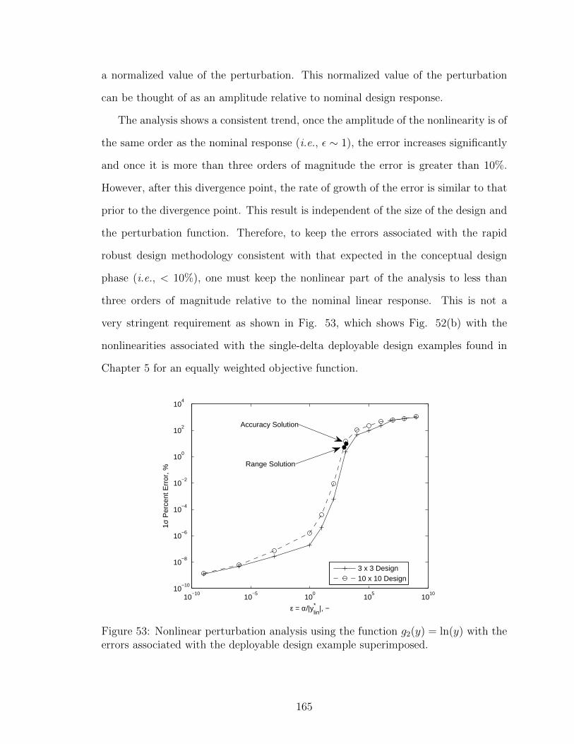
a normalized value of the perturbation. This normalized value of the perturbation
can be thought of as an amplitude relative to nominal design response.
The analysis shows a consistent trend, once the amplitude of the nonlinearity is of
the same order as the nominal response (i.e., ε ∼ 1), the error increases significantly
and once it is more than three orders of magnitude the error is greater than 10%.
However, after this divergence point, the rate of growth of the error is similar to that
prior to the divergence point. This result is independent of the size of the design and
the perturbation function. Therefore, to keep the errors associated with the rapid
robust design methodology consistent with that expected in the conceptual design
phase (i.e., < 10%), one must keep the nonlinear part of the analysis to less than
three orders of magnitude relative to the nominal linear response. This is not a
very stringent requirement as shown in Fig. 53, which shows Fig. 52(b) with the
nonlinearities associated with the single-delta deployable design examples found in
Chapter 5 for an equally weighted objective function.
10−10
10−5
100
105
1010
10−10
10−8
10−6
10−4
10−2
100
102
104
ε = α/|y*lin
|, −
1σ P
erce
nt E
rror
, %
3 x 3 Design10 x 10 Design
Range Solution
Accuracy Solution
Figure 53: Nonlinear perturbation analysis using the function g2(y) = ln(y) with theerrors associated with the deployable design example superimposed.
165
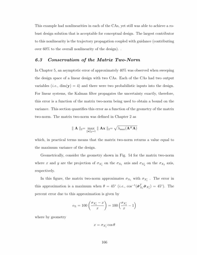
This example had nonlinearities in each of the CAs, yet still was able to achieve a ro-
bust design solution that is acceptable for conceptual design. The largest contributor
to this nonlinearity is the trajectory propagation coupled with guidance (contributing
over 60% to the overall nonlinearity of the design). .
6.3 Conservatism of the Matrix Two-Norm
In Chapter 5, an asymptotic error of approximately 40% was observed when sweeping
the design space of a linear design with two CAs. Each of the CAs had two output
variables (i.e., dim(y) = 4) and there were two probabilistic inputs into the design.
For linear systems, the Kalman filter propagates the uncertainty exactly, therefore,
this error is a function of the matrix two-norm being used to obtain a bound on the
variance. This section quantifies this error as a function of the geometry of the matrix
two-norm. The matrix two-norm was defined in Chapter 2 as
‖ A ‖2= max‖x‖2=1
‖ Ax ‖2=√λmax(AHA)
which, in practical terms means that the matrix two-norm returns a value equal to
the maximum variance of the design.
Geometrically, consider the geometry shown in Fig. 54 for the matrix two-norm
where x and y are the projection of σX′1 on the σX1 axis and σX′2 on the σX2 axis,
respectively.
In this figure, the matrix two-norm approximates σX1 with σX′1 . The error in
this approximation is a maximum when θ = 45 (i.e., cos−1(σTX1σX′1) = 45). The
percent error due to this approximation is given by
ε% = 100
(σX′1 − x
x
)= 100
(σX′1x− 1)
where by geometry
x = σX′1 cos θ
166
1X
2X
'1X
'2X
2Σ
y
x
Figure 54: Two-dimensional geometry associated with the matrix two-norm.
Therefore, the expression for error can be reduced to
ε% = 100
(1
cos θ− 1
)When substituting in θ = 45, this yields a percent error of 41.42% in the estimation
of the standard deviation for the two-dimensional problem of Fig. 54. This result
can be generalized to accommodate growth in the dimensionality of the covariance
matrix. As the dimensionality of the covariance matrix increases, the value of ε%
decreases due to changes in the geometry of the design space changing θ. This is
shown in Fig. 55.
In Fig. 55, for the case of four CA outputs, as was used in Chapter 5, this error
produces a 37.8% error, which is the error observed in the parameter sweep in Figs.
18-20. Even with a large number of design variables, the two-norm approximation to
the standard deviation produces a 20 − 25% conservative approximation. However,
this will only be achieved in cases where there is loose coupling between CAs.
167
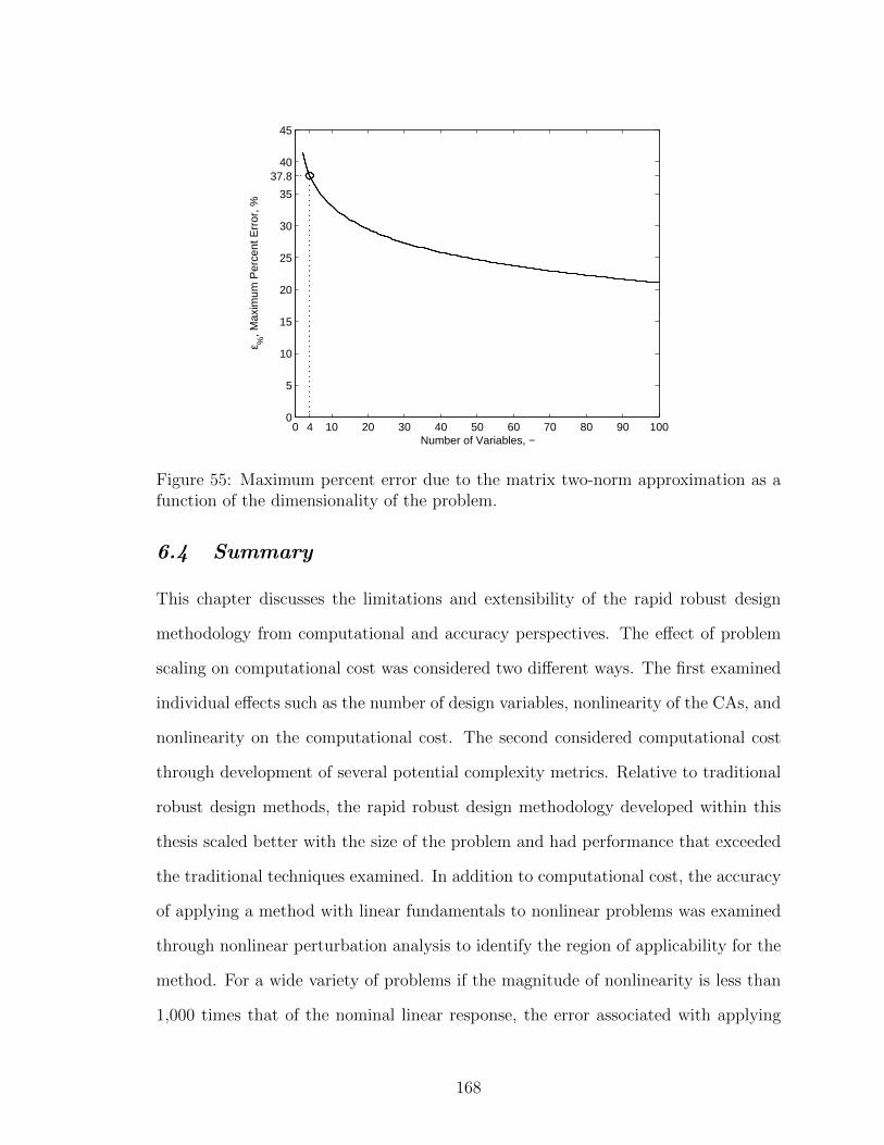
0 4 10 20 30 40 50 60 70 80 90 1000
5
10
15
20
25
30
35
37.840
45
Number of Variables, −
ε %, M
axim
um P
erce
nt E
rror
, %
Figure 55: Maximum percent error due to the matrix two-norm approximation as afunction of the dimensionality of the problem.
6.4 Summary
This chapter discusses the limitations and extensibility of the rapid robust design
methodology from computational and accuracy perspectives. The effect of problem
scaling on computational cost was considered two different ways. The first examined
individual effects such as the number of design variables, nonlinearity of the CAs, and
nonlinearity on the computational cost. The second considered computational cost
through development of several potential complexity metrics. Relative to traditional
robust design methods, the rapid robust design methodology developed within this
thesis scaled better with the size of the problem and had performance that exceeded
the traditional techniques examined. In addition to computational cost, the accuracy
of applying a method with linear fundamentals to nonlinear problems was examined
through nonlinear perturbation analysis to identify the region of applicability for the
method. For a wide variety of problems if the magnitude of nonlinearity is less than
1,000 times that of the nominal linear response, the error associated with applying
168

successive linearization will result in 1σ errors in the response less than 10% compared
to the full nonlinear error. Conservatism due to the use of the matrix two-norm was
also examined through assessment of the asymptotic error that was first observed in
Chapter 5. This error was shown to be the result of design geometry and is reduced
as the dimensionality of y (i.e., the number of outputs from the CAs) increases.
169
CHAPTER VII
SUMMARY AND FUTURE WORK
7.1 Summary of Academic Contributions
This thesis advances the state-of-the-art in the analysis and design of multidisci-
plinary systems by developing and applying concepts from dynamical systems theory
to the conceptual design process. Three techniques from dynamical system theory—
stability analysis, constraint handling, and estimation theory—are shown to provide
advantages compared to traditional design techniques. Building on these techniques,
a rapid robust design methodology is developed for linear multidisciplinary design.
While the developed methodology is inherently linear, it was shown to be applicable
to nonlinear engineering problems through successive linearization.
7.1.1 Formulation of the General Multidisciplinary Design Problem asa Dynamical System In Order to Leverage Established Techniquesfrom Dynamical System Theory
The design of multidisciplinary systems requires analyses from numerous disciplines in
order to achieve a set of objectives. A converged candidate design is one in which each
of the disciplines uses the same information, has a common set of assumptions, and
satisfies the problem constraints. An optimal design can be selected from the set of
converged candidates. These processes are traditionally computationally burdensome.
By leveraging advances in dynamical system theory, solution of the multidisciplinary
design process is shown to be more computationally tractable as well as yielding
robustness insight into the problem.
Finding a converged multidisciplinary design can be thought of as a multidimen-
sional root-finding problem (e.g., the process of finding x∗ such that f(x∗) = 0). In
170
this case, the x being sought are the outputs of each of the CAs in the design and the
function, f(·), is the difference between the assumed values of the CAs output and the
actual values of the output. The solution process to identify the roots of the design
can be framed as an iterative one, where the subsequent iteration relies on informa-
tion from prior iterates. Since a dynamical system is defined by two characteristics:
(1) a state and (2) a fixed-rule describing the evolution of the state, the root-finding
iteration scheme can be thought of as a dynamical system, where the CAs output is
the state and the root-finding scheme is the fixed-rule.
7.1.2 Application of the Dynamical System Domain to the Multidisci-plinary Design Problem
Three dynamical system techniques were investigated for the benefits they could
provide to multidisciplinary design as well as their use as an ensemble in development
of a rapid robust design methodology.
7.1.2.1 Stability Analysis
Typically, there is little indication beyond designer experience at the beginning of
the design-analysis cycle regarding the existence of a converged design that meets
the design specifications. Such was the case in the NASA Constellation program
where select requirements were relaxed or ignored[204]. Stability theory can be used
to rectify this problem by providing insight into the existence of a design based on
the convergence procedure being utilized. For a design to exist, it was shown that
when using iterative convergence techniques (e.g., fixed-point iteration), the iteration
scheme used to converge the design must be asymptotically stable. For linear, con-
stant coefficient systems, this was shown to be readily checked through evaluation of
the eigenvalues. However, for more general designs, existence of a converged design
was shown to be obtainable through the use of Lyapunov techniques. These tech-
niques were shown to be able to identify domains for which initial guesses result in
171
converged, feasible designs as well as to access the rate of convergence. This allows a
priori knowledge regarding the design space, specifically whether a design is capable
of being found as well as how fast it can be found. Lyapunov techniques rely on iden-
tification of a Lyapunov function for analysis. Identifying this Lyapunov function,
in general, can be challenging; however, this work demonstrated that sum-of-squares
analysis can be used to obtain this function. This technique allows a Lyapunov func-
tion to be found for systems (including those with unknown variables) that can be
factored into a sum-of-squares. This is shown to be computationally efficient through
application of standard semi-definite programming tools. For exponentially stable
designs, it was shown that further analysis can be applied to the Lyapunov function
to identify the rate at which the design will converge.
7.1.2.2 Control Theory
Optimal control techniques were demonstrated in this thesis to allow equality and
inequality constraints to be included in the design procedure. These techniques allow
for the consideration of design variable constraints and constraints on the output of
each CA to be considered at the same level in the design hierarchy. This is a departure
from the majority of MDO techniques, where only constraints that are a function of
the design variables are considered explicitly at the system level. By applying these
constraints at the same level in the optimization hierarchy, a coordinated search of
the design space ensues which may lead to efficiency in the design process.
7.1.2.3 Estimation Techniques
Estimation theory is used in this work to obtain a rapid estimate of the mean and
variance of the design. The Kalman filter, when modified to resemble those formed
in linear covariance analysis, is propagated alongside the iteration relationship, pro-
viding a simultaneous estimate of the mean and covariance of the CAs’ output. This
was shown to have significant computational advantages as opposed to traditional
172
uncertainty quantification techniques such as Monte Carlo simulation, the unscented
transform, and FPI. To achieve this estimate requires propagating seven additional
equations as opposed to traditional methods which require drawing from a distribu-
tion and converging the design for that set of uncertainty values or building successive
approximate functions to the response. Furthermore, since the correlation coefficient
for each output of the CAs can be obtained directly from the resulting covariance
matrix it can be used to guide design decomposition. In this approach, correla-
tion coefficients larger in magnitude are more significant in the response and as such
should always be included. However, variables with smaller correlation coefficient
magnitudes may be eliminated from the feedback structure of a design.
7.1.3 Development of a Linear Technique for the Rapid Robust Designof a Multidisciplinary System
A method for robustness assessment and identification of a robust design that bounds
the variance using a matrix norm of the covariance matrix was also developed in
this thesis. This technique was developed for linear systems and was shown to be
readily extensible to nonlinear systems. This methodology was applied to a wide
variety of problems that ranged from algebraic examples to aerospace applications,
demonstrating the broad applicability of the developed techniques to a number of
fields. Significant computational performance gains of the developed technique were
demonstrated with a reduction in the number of function calls by a factor of two when
compared to the unscented transform and more than an order of magnitude when
compared to FPI and Monte Carlo techniques with minimal sacrifices to the accuracy
(< 3%). It was shown that the methodology could accommodate nonlinearity with
an order of magnitude less than 100 times the nominal value of the CA response.
Finally, conservatism associated with use of the matrix two-norm showed that the
error bounding the variance is a result of geometry and is reduced as the number of
outputs from the CAs increases.
173
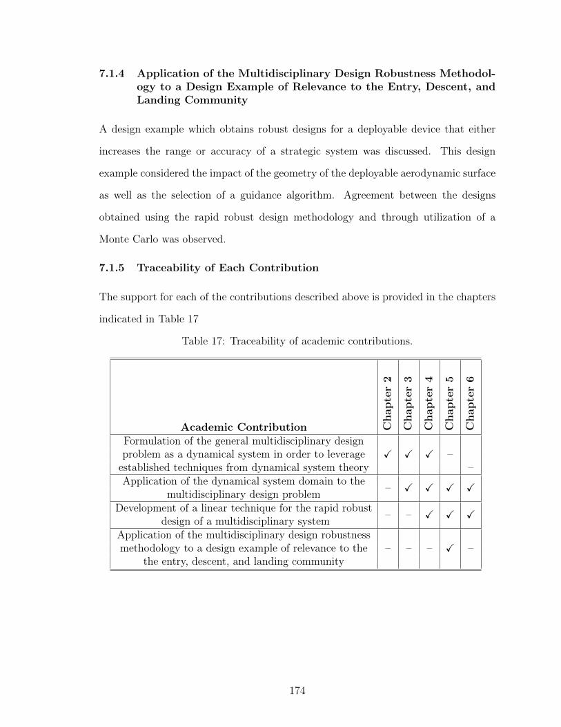
7.1.4 Application of the Multidisciplinary Design Robustness Methodol-ogy to a Design Example of Relevance to the Entry, Descent, andLanding Community
A design example which obtains robust designs for a deployable device that either
increases the range or accuracy of a strategic system was discussed. This design
example considered the impact of the geometry of the deployable aerodynamic surface
as well as the selection of a guidance algorithm. Agreement between the designs
obtained using the rapid robust design methodology and through utilization of a
Monte Carlo was observed.
7.1.5 Traceability of Each Contribution
The support for each of the contributions described above is provided in the chapters
indicated in Table 17
Table 17: Traceability of academic contributions.
Academic Contribution Ch
ap
ter
2
Chap
ter
3
Ch
ap
ter
4
Chapte
r5
Chapte
r6
Formulation of the general multidisciplinary designX X X –
–problem as a dynamical system in order to leverage
established techniques from dynamical system theoryApplication of the dynamical system domain to the
– X X X Xmultidisciplinary design problem
Development of a linear technique for the rapid robust– – X X X
design of a multidisciplinary systemApplication of the multidisciplinary design robustness
– – – X –methodology to a design example of relevance to thethe entry, descent, and landing community
174
7.2 Advantages of Viewing the Multidisciplinary DesignProblem as a Dynamical System
Viewing the multidisciplinary design problem as a dynamical systems improves the
design knowledge, broadens the computational tools, and reduces the computational
burden in the design-analysis cycle.
• Increase in Design Knowledge: Applying stability theory allows the iden-
tification of whether or not a feasible design exists for a given iteration scheme
and knowledge regarding how that design is approached. A priori knowledge of
this information can be used by the designer to examine the design space sensi-
tivities as well as gives an estimate of the time to obtain a design. In addition,
this information can be leveraged in a distributed work environment to provide
an estimate of the level of accuracy that is achievable for a given number of
data transfers.
• Broadens Computational Tools: Using optimal control theory allows for
constraints that are functions of both the CA output and the design variables
to be considered at the same level of the optimization hierarchy. This allows
the search for an optimal solution from a reduced design space, potentially
enabling efficiencies in the design process. Estimation theory can also be used
in a manner similar to linear covariance analysis to provide an estimate of the
mean and covariance of the CA’s output (and their effect on the design response)
at the same time as the design is found.
• Reduces Computational Burden: Several solution methods that are pri-
marily used within the dynamical system community were described within
this thesis. These include sum-of-squares analysis for stability analysis, use of
discrete and continuous optimal control solutions, and the Kalman filter. Ef-
ficient solution procedures for these methods exist, such as those described in
175
Refs. [147, 131, 205]. As shown in Chapters 5 and 6, application of these
methods can provide solutions faster than those of current MDO techniques.
These advantages along with the comparable accuracy complement the existing con-
ceptual design techniques such as surrogate modeling and design of experiments.
7.3 Limitations of the Rapid Robust Design Methodology
The rapid robust design methodology developed in Chapter 4 has several limitations
due to the assumptions associated with its development. These include:
1. Linear technique: The application of the Kalman filter is exact only for linear
dynamical systems. However, as in this methodology, the Kalman filter can
be extended to nonlinear systems through successive linearization which may
induce an error in the estimate of the mean and covariance of the response.
As shown in Chapters 5 and 6, this is not a strong limitation of the technique.
The successive linearization procedure induces errors that are less than 1% as
long as the nonlinear perturbation is less than the magnitude of the linear CAs’
response.
2. Scalar objective function: As formulated, the rapid robust design method-
ology requires a single, scalar objective function. As mentioned in Chapter 1,
design is usually a multi-objective problem. Therefore in order to account for
the multi-objective nature of design an aggregate objective function such as
J =∑
Ω
wiJ ni (124)
needs to be formed in order to seek the Pareto frontier. In Eq. (124), Ω is the
set of objective functions, wi are weights on the objective functions, Ji is the
individual objective function, and n ∈ R+∪∞\0 is the power of the objective
function. A limitation of this technique is that aggregate objective functions
176

are known to omit concave parts of the frontier, which limits the techniques
ability to find to full set of Pareto optimal designs[206].
3. Iteration scheme: If the application of the stability analysis portion of the
rapid robust design methodology fails to show at least asymptotic stability it
does not necessarily mean that a design does not exist. Instead, it implies
that for the given iteration scheme chosen, a design cannot be found. In these
instances alternative iteration schemes should be investigated.
4. Variance bound: The matrix two-norm of the covariance matrix was in-
voked in order to meet the scalar objective function limitation presented in
this methodology. While the two-norm provides a conservative bound on the
variance of the design’s response with estimates that are no more than 42%
that of the actual design response’s standard deviation, it is provides a source
of error in the solutions of the rapid robust design methodology.
5. Gaussian uncertainties: The derivation of the Kalman filter assumes Gaus-
sian distributions of the uncertainties[158]. Since the Kalman filter is utilized in
this work, the Gaussian distribution assumption is also applicable to this work.
7.4 Suggestions for Future Work
The work presented within this thesis has shown the applicability of dynamical sys-
tems techniques to the multidisciplinary design problem. In particular three areas
of dynamical system theory were explored as they relate to the the development of
a rapid robust multidisciplinary design methodology. Some suggested avenues for
future work are described below—additional dynamical systems techniques that have
potential applicability to the multidisciplinary design problem and potential tech-
niques to extend and overcome some of the limitations of the rapid robust design
methodology.
177
7.4.1 Additional Dynamical Systems Techniques
The formulation of the multidisciplinary design problem as a dynamical system lends
itself to application of a large variety of dynamical systems techniques. These tech-
niques can be used to analyze and extend knowledge regarding the multidisciplinary
design problem. In addition, these methods could be used to formalize already existing
procedures and methodologies within the multidisciplinary analysis and optimization
community.
The stability aspect of dynamical system theory was discussed in Chapter 3 where
convergence conditions for constant coefficient, linear designs were identified using
eigenvalue analysis and more general designs were identified using Lyapunov the-
ory. However, Lyapunov theory has its limitations. In particular, if a Lyapunov
function cannot be found, then nothing can be said regarding whether the design
will ultimately converge. While this proved not to be an issue for any of the ex-
ample problems examined within this thesis, this characteristic ultimately limits the
utility of Lyapunov theory. Analyzing the invariant manifolds associated with con-
verged designs is one possible path to overcome the shortcoming of Lyapunov theory.
By identifying the stable invariant manifold, a path to a converged design can be
identified and as long as the iteration intersects this manifold, convergence can be
assured[207]. This technique is commonly used within the astrodynamics community
to identify transfers within the three-body problem[208].
Convergence properties of multidisciplinary designs were analyzed in this work for
a specific subset of problems—design iterations that can be shown to be exponentially
stable through Lyapunov analysis. However, other information about convergence
behavior can be identified through alternative means. For example, Fourier analysis,
which is used in computational fluid dynamics to identify the convergence properties
of finite difference solutions to partial differential equations, could be employed[209].
Similarly, for linear systems, the z-transform can be used to transform the analysis
178
domain. In particular, the stability of a system in the z-plane can be determined
by looking at its trace in the z-plane. Namely, if all of the poles of the transfer
function lie within the unit circle then the discrete system is stable[210, 141, 132].
Furthermore, for this restricted class of systems, additional characteristics such as
rise time and overshoot can be characterized.
It was observed in Chapters 3 and 5 that indirect and direct continuous optimal
control solutions provided similar results as the discrete optimal control problem.
The reason for this is the more restrictive conditions associated with the solution to
the continuous problem which are a subset of the discrete optimal control problem.
However, the issue of time-horizon was not addressed, which can be further investi-
gated. Another area for further exploration within the control world is how to ensure
that the constraints are convex. For the problems examined in Chapter 5, the con-
straints were convex by formulation. However, for general design problems this may
not be achievable requiring techniques such as second-order cone theory to be used
to convexify the constraint[211, 212].
Finally, in the area of estimation theory additional methods to propagate uncer-
tainty could be incorporated. For this work, theoretical development was restricted
to linear designs which lend themselves to the use of the Kalman filter. However,
design is nonlinear, as demonstrated in Chapters 5 and 6. While the techniques
developed within this thesis were shown yield accurate estimates of the mean and
covariance for all but the most nonlinear of designs, other estimation techniques
may be more efficient and more accurate. These estimation techniques include the
Extended Kalman filter, which formalizes the successive linearization process imple-
mented in this work, the Unscented Kalman filter, which uses the unscented transform
instead of the linearized dynamics to propagate the uncertainty, and the particle fil-
ter, which propagates a small number of samples to obtain the mean and variance
at each iteration[162, 213]. In addition, the rapid assessment of uncertainty allows
179
the contributors to the design’s uncertainty to be examined rapidly. This could be
accomplished in a traditional manner by perturbing the design variables to obtain the
sensitivities. However, as the full covariance analysis is available to the designer, the
individual CA response contributions to the uncertainty can be readily ascertained
as is performed in Ref. [84].
While this work was limited to the multidisciplinary design problem, dynamical
system theory has potential application in the design and optimization community at
large. For instance, stability analysis could be applied to an optimization algorithm
directly to identify whether or not the algorithm will obtain an optimal design and the
speed at which it can do so. As such, this information can be leveraged in the design
of optimization algorithms to ensure solutions are obtained efficiently. Similarly,
these techniques have further applicability to traditional MDO techniques such as
optimizer based decomposition, where the optimizer handles the design convergence,
allowing knowledge regarding the behaviors of these methodologies to be obtained
and leveraged.
In addition, the dynamical system field is rich with elements that could be used to
study design including chaos theory, ergodic theory, functional analysis, graph theory,
and topology theory. Each of these areas has numerous techniques that offer potential
to better understand the design problem.
7.4.2 Extending the Use of the Rapid Robust Design Methodology
In the derivation of the methodology, a strong underlying assumption of employing
the Kalman filter in the analysis is that the uncertain inputs and parameters are
Gaussian distributed. This is because the Kalman filter only propagates the first
and second moments (i.e., the mean and variance) which fully describe the normal
distribution. This assumption also holds well for symmetric probability distributions;
however, for asymmetric distributions it breaks down relatively rapidly[214]. Methods
180

such as a particle filtering enable the propagation of various probability distributions,
but they do so at the expense of computational speed. A potential solution to this
problem would be to borrow from control theory and look at implementing a robust
or stochastic control algorithm[215, 216]. These techniques use assumptions of the
behavior of noise variables to make sure that a solution is reached. Alternatively,
investigation of a Gaussian-mixture type formulation (as is done in Ref. [98]) may
allow for a broader class of uncertainties to be accommodated within the developed
framework.
As formulated in this dissertation, the rapid robust design methodology lends it-
self to potential integration with an integrated design environment such as Phoenix
Integration’s ModelCenter or Simulia’s iSIGHT[217, 218]. These environments pro-
vide a general wrapping environment to provide a design analysis and optimization
framework for various types of CAs that can be substituted and changed. In such
an environment, the rapid robust design methodology could be readily applied to
provide computationally tractable, robust optimal designs for arbitrary designs with
CAs provided by standalone applications.
Another avenue for future work would be to add the capability to analyze a com-
bination of algebraic and dynamical CAs. For aerospace applications this capability
could be used to simultaneously design the guidance, navigation, and control (GN&C)
system with the trajectory and the vehicle. The design of the GN&C system is usually
accomplished subsequent to the preliminary design of the vehicle resulting in signifi-
cant iteration to approach an optimal design with respect to the true system metrics.
By pulling forward the GN&C design such that it is conducted simultaneously with
other aspects of the vehicle design, CA interactions are appropriately modeled. Syn-
thesis of the vehicle characteristics simultaneously with the GN&C system may allow
a robust solution to be obtained that improves aspects of the trajectory through
modification of vehicle characteristics and vice-versa.
181
APPENDIX A
SELECT MATHEMATICAL CONCEPTS
A.1 Probability and Statistics
A.1.1 Probability Space and Random Variables
Probability space is a model for real world situations in which the outcome is assigned
according to some probability. It is a measure space such that the measure of the
whole space is equal to unity and is defined as[219]
Definition: Probability Space
Probability space is a triple, (Ω,F , P ), consisting of the following elements:
• Sample space (Ω): a representation of all possible outcomes (Ω 6= ∅)
• Event space (F): a collection of subsets of Ω such that
– The null set is an element of the event space: ∅ ∈ F– The event space is closed under complements: if A ∈ F , then
(Ω\A) ∈ F– The event space is closed under countable unions: if Ai ∈ F fori = 1, 2, ..., then (∪Ai) ∈ F
• Probability measure (P ): A function P : F → [0, 1] such that
– The probability measure is non-negative: P (A) ≥ 0, ∀A ∈ F– The probability measure is countably additive: P (Ai∪Aj) = P (Ai)+P (Aj) if Ai ∩Aj = ∅, ∀Ai, Aj ∈ F
– The measure of the entire sample space is unity: P (Ω) = 1
With the concept of probability space defined, the formal definition of random
variables can be given[220].
182
Definition: Random Variable
Let (Ω,F , P ) be a probability space and (Y,Σ) be a measurable space. Then arandom variable X is a measurable function X : Ω→ Y .
A random variable can be interpreted as the preimages of the well-behaved subsets of
Y (the elements of Σ) are events (i.e., elements of F), are are assigned a probability
by P . Or, more simply, a random variable is a function whose domain is the sample
space and maps events to real numbers.
A.1.2 Univariate Probability Density and Distribution Functions
For an univariate discrete random variable, a probability distribution assigns a prob-
ability for each of value of the random variable, while for a continuous univariate
random variable, the probability distribution gives the probability of the value falling
within a particular interval. Formally, a univariate probability distribution is defined
as[220]
Definition: Probability Distribution
For a random variable, X : Ω→ Y , a probability distribution is the pushforwardmeasure X∗P = PX−1 on (Y,Σ).
More tangibly, for real-valued random variables, the probability of a random variable
X being in the interval (−∞, x] is given by the cumulative distribution function
F (x) = P (X ≤ x), ∀x ∈ R (A.1.1)
A.1.2.1 Discrete Random Variables
For discrete probability distributions (i.e., the sample space, Ω, consists entirely of
values that are in a countable predefined set), the probability is characterized by a
183
probability mass function, f(x), which is defined by the relationship
∑x∈Ω
P (X = x) =∑x∈Ω
f(x) = 1 (A.1.2)
In addition, the probability mass function has the property
0 ≤ f(x) ≤ 1 (A.1.3)
The cumulative distribution function associated with discrete random variables is
such that there are jump discontinuities. Between these jump discontinuities, since
there is no additional probability as defined in Eq. (A.1.1), the value of the function
is constant.
A.1.2.2 Continuous Random Variables
For continuous random variables (i.e., the sample space, Ω, can consist of any subset
R), the cumulative distribution function is defined in terms of an integral instead of
a summation as shown in Eq. (A.1.4)
F (x) = P (X ≤ x) =
x∫−∞
f(u)du (A.1.4)
where f(x) is the probability density function. The probability density function gives
the probability of a given value and is defined in terms of the cumulative distribution
function as
f(x) =d
dxF (x) (A.1.5)
Since the cumulative distribution function is a strictly increasing function, the proba-
bility density function, f(x), is a non-negative function whose integral over the entire
sample space is equal to unity.
A.1.3 Multivariate Probability Density and Distribution Functions
Assume n (n <∞) random variables X1, X2, . . . , Xn are defined on the same probabil-
ity space (Ω,F , P ). The cumulative distribution function of this bivariate distribution
184
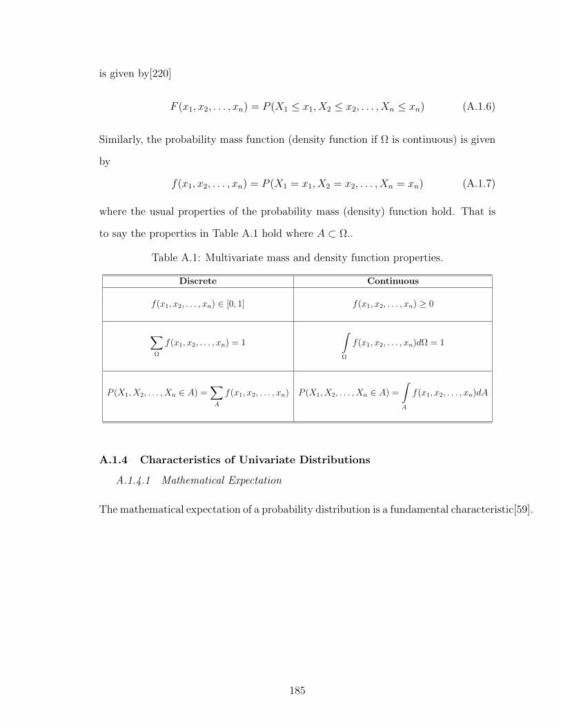
is given by[220]
F (x1, x2, . . . , xn) = P (X1 ≤ x1, X2 ≤ x2, . . . , Xn ≤ xn) (A.1.6)
Similarly, the probability mass function (density function if Ω is continuous) is given
by
f(x1, x2, . . . , xn) = P (X1 = x1, X2 = x2, . . . , Xn = xn) (A.1.7)
where the usual properties of the probability mass (density) function hold. That is
to say the properties in Table A.1 hold where A ⊂ Ω..
Table A.1: Multivariate mass and density function properties.
Discrete Continuous
f(x1, x2, . . . , xn) ∈ [0, 1] f(x1, x2, . . . , xn) ≥ 0
∑Ω
f(x1, x2, . . . , xn) = 1
∫Ω
f(x1, x2, . . . , xn)dΩ = 1
P (X1, X2, . . . , Xn ∈ A) =∑A
f(x1, x2, . . . , xn) P (X1, X2, . . . , Xn ∈ A) =
∫A
f(x1, x2, . . . , xn)dA
A.1.4 Characteristics of Univariate Distributions
A.1.4.1 Mathematical Expectation
The mathematical expectation of a probability distribution is a fundamental characteristic[59].
185
Definition: Mathematical Expectation
If f(x) is the probability mass (density) function for a random variable X ofthe discrete (continuous) type, then the mathematical expectation of a functionu(x) is defined as
E[u(x)] =∑x∈Ω
u(x)f(x)
for discrete distributions and
E[u(x)] =
∞∫−∞
u(x)f(x)dx
for continuous distributions provided they exist and are finite.
From this definition, it is clear to see that the expectation is a linear operator.
A.1.4.2 The Moment Generating Function
For the majority of distributions whose densities are given analytically, it is useful to
consider the moment generating function[59].
Definition: Moment Generating Function
The moment generating function for a distribution whose probability mass (den-sity) function is defined by f(x) is given by
M(t) = E(etX)
provided it exists and is finite for some t ∈ [−h, h].
To examine the impact of the moment generating function, consider the discrete case
where the sample space Ω consists of ω1, ω2, ω3, . . . then
M(t) = etω1f(ω1) + etω2f(ω2) + etω3f(ω3) + . . .
and hence the coefficient of etωi is the probability
f(ωi) = P (X = ωi)
186
Therefore, since this probability is prescribed only to this distribution, the moment
generating function describes a unique distribution, if it exists.
A.1.4.3 The Mean
The mean (or average) is a fundamental quantity that describes the expected value
of the distribution, it is also the first moment.
Definition: Mean
The mean of a random variable X is given by
µ = E[X]
This is also expressed in terms of the moment generating function (when itexists) as
µ =dM
dt(0)
A.1.4.4 The Variance
The variance is another measure of central tendency that describes the spread of val-
ues from the mean of the distribution.
Definition: Variance
The variance of a random variable X is given by
σ2 = E[(X − µ)2]
This is also expressed in terms of the moment generating function (when itexists) as
σ2 =d2M
dt2(0)−
[dM
dt(0)
]2
A larger variance (standard deviation) implies that the spread of the distribution is
larger than that of a smaller variance.
187
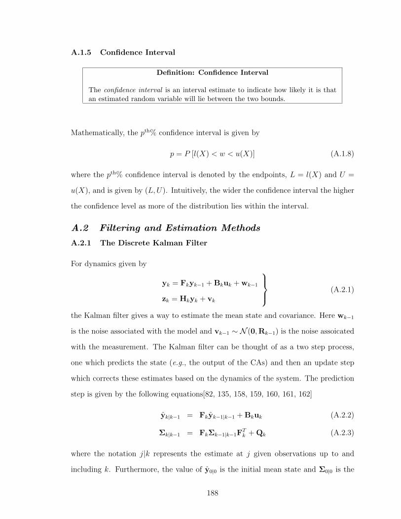
A.1.5 Confidence Interval
Definition: Confidence Interval
The confidence interval is an interval estimate to indicate how likely it is thatan estimated random variable will lie between the two bounds.
Mathematically, the pth% confidence interval is given by
p = P [l(X) < w < u(X)] (A.1.8)
where the pth% confidence interval is denoted by the endpoints, L = l(X) and U =
u(X), and is given by (L,U). Intuitively, the wider the confidence interval the higher
the confidence level as more of the distribution lies within the interval.
A.2 Filtering and Estimation Methods
A.2.1 The Discrete Kalman Filter
For dynamics given by
yk = Fkyk−1 + Bkuk + wk−1
zk = Hkyk + vk
(A.2.1)
the Kalman filter gives a way to estimate the mean state and covariance. Here wk−1
is the noise associated with the model and vk−1 ∼ N (0,Rk−1) is the noise assoicated
with the measurement. The Kalman filter can be thought of as a two step process,
one which predicts the state (e.g., the output of the CAs) and then an update step
which corrects these estimates based on the dynamics of the system. The prediction
step is given by the following equations[82, 135, 158, 159, 160, 161, 162]
yk|k−1 = Fkyk−1|k−1 + Bkuk (A.2.2)
Σk|k−1 = FkΣk−1|k−1FTk + Qk (A.2.3)
where the notation j|k represents the estimate at j given observations up to and
including k. Furthermore, the value of y0|0 is the initial mean state and Σ0|0 is the
188
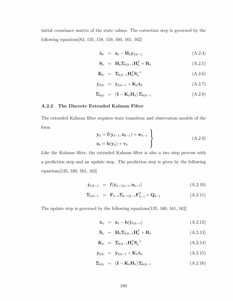
initial covariance matrix of the state values. The correction step is governed by the
following equations[82, 135, 158, 159, 160, 161, 162]
xk = zk −Hkyk|k−1 (A.2.4)
Sk = HkΣk|k−1HTk + Rk (A.2.5)
Kk = Σk|k−1HTkS−1
k (A.2.6)
yk|k = yk|k−1 + Kkxk (A.2.7)
Σk|k = (I−KkHk) Σk|k−1 (A.2.8)
A.2.2 The Discrete Extended Kalman Filter
The extended Kalman filter requires state transition and observation models of the
form
yk = f(yk−1,uk−1) + wk−1
zk = h(yk) + vk
(A.2.9)
Like the Kalman filter, the extended Kalman filter is also a two step process with
a prediction step and an update step. The prediction step is given by the following
equations[135, 160, 161, 162]
yk|k−1 = f(yk−1|k−1,uk−1) (A.2.10)
Σk|k−1 = Fk−1Σk−1|k−1FTk−1 + Qk−1 (A.2.11)
The update step is governed by the following equations[135, 160, 161, 162]
xk = zk − h(yk|k−1) (A.2.12)
Sk = HkΣk|k−1HTk + Rk (A.2.13)
Kk = Σk|k−1HTkS−1
k (A.2.14)
yk|k = yk|k−1 + Kkxk (A.2.15)
Σk|k = (I−KkHk) Σk|k−1 (A.2.16)
189
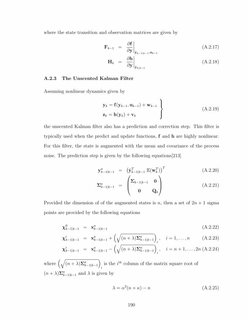
where the state transition and observation matrices are given by
Fk−1 =∂f
∂y
∣∣∣∣yk−1|k−1,uk−1
(A.2.17)
Hk =∂h
∂y
∣∣∣∣yk|k−1
(A.2.18)
A.2.3 The Unscented Kalman Filter
Assuming nonlinear dynamics given by
yk = f(yk−1,uk−1) + wk−1
zk = h(yk) + vk
(A.2.19)
the unscented Kalman filter also has a prediction and correction step. This filter is
typically used when the predict and update functions, f and h are highly nonlinear.
For this filter, the state is augmented with the mean and covariance of the process
noise. The prediction step is given by the following equations[213]
yak−1|k−1 =(yTk−1|k−1 E(wT
k ))T
(A.2.20)
Σak−1|k−1 =
Σk−1|k−1 0
0 Qk
(A.2.21)
Provided the dimension of of the augmented states is n, then a set of 2n + 1 sigma
points are provided by the following equations
χ0k−1|k−1 = xak−1|k−1 (A.2.22)
χik−1|k−1 = xak−1|k−1 +(√
(n+ λ)Σak−1|k−1
)i, i = 1, . . . , n (A.2.23)
χik−1|k−1 = xak−1|k−1 −(√
(n+ λ)Σak−1|k−1
)i, i = n+ 1, . . . , 2n (A.2.24)
where(√
(n+ λ)Σak−1|k−1
)i
is the ith column of the matrix square root of
(n+ λ)Σak−1|k−1 and λ is given by
λ = α2(n+ κ)− n (A.2.25)
190
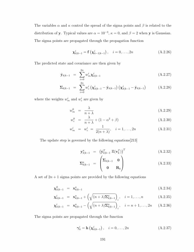
The variables α and κ control the spread of the sigma points and β is related to the
distribution of y. Typical values are α = 10−3, κ = 0, and β = 2 when y is Gaussian.
The sigma points are propagated through the propagation function
χik|k−1 = f(χik−1|k−1
), i = 0, . . . , 2n (A.2.26)
The predicted state and covariance are then given by
yk|k−1 =2n∑i=0
wimχik|k−1 (A.2.27)
Σk|k−1 =2n∑i=0
wic(χik|k−1 − yk|k−1
) (χik|k−1 − yk|k−1
)(A.2.28)
where the weights wim and wic are given by
w0m =
λ
n+ λ(A.2.29)
w0c =
λ
n+ λ+ (1− α2 + β) (A.2.30)
wim = wic =1
2(n+ λ), i = 1, . . . , 2n (A.2.31)
The update step is governed by the following equations[213]
yak|k−1 =(yTk|k−1 E(vTk )
)T(A.2.32)
Σak|k−1 =
Σk|k−1 0
0 Rk
(A.2.33)
A set of 2n+ 1 sigma points are provided by the following equations
χ0k|k−1 = xak|k−1 (A.2.34)
χik|k−1 = xak|k−1 +(√
(n+ λ)Σak|k−1
)i, i = 1, . . . , n (A.2.35)
χik|k−1 = xak|k−1 −(√
(n+ λ)Σak|k−1
)i, i = n+ 1, . . . , 2n (A.2.36)
The sigma points are propagated through the function
γik = h(χik|k−1
), i = 0, . . . , 2n (A.2.37)
191

With the weights defined in the prediction step, the weighted sigma points are then
used to produce the predicted measurement and the measurement correction
zk|k−1 =2n∑i=0
wimγik (A.2.38)
Σzkzk =2n∑i=0
wic(γik − zk
) (γik − zk
)T(A.2.39)
The matrix
Σykzk =2n∑i=0
wic(χik|k−1 − xk|k−1
) (γik − zk
)T(A.2.40)
is used to compute the gain
Kk = ΣykzkΣ−1zkzk
(A.2.41)
which is used to compute the updated state
yk|k = yk|k−1 + Kk(zk − zk) (A.2.42)
Σk|k = Σk|k−1 −KkΣzkzkKTk (A.2.43)
A.3 Uncertainty Propagation Techniques
A.3.1 Analytic Propagation in Linear Systems
Consider an input-output relationship for an analysis of the following form[59]
Y = AX (A.3.1)
where A is a scalar matrix and X is a vector of random variables with mean µX and
covariance matrix ΣX. The mean for this combination is given by
µY = AµX (A.3.2)
and the covariance for this linear relationship is given by
ΣY = AΣXAT (A.3.3)
Hence, if the mean and covariance of the input variables are known, the mean and
covariance matrix of the output of the analysis can be determined analytically for the
case of a linear input-output relationship.
192
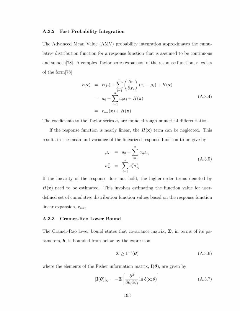
A.3.2 Fast Probability Integration
The Advanced Mean Value (AMV) probability integration approximates the cumu-
lative distribution function for a response function that is assumed to be continuous
and smooth[78]. A complex Taylor series expansion of the response function, r, exists
of the form[78]
r(x) = r(µ) +n∑i=1
(∂r
∂xi
)(xi − µi) +H(x)
= a0 +n∑i=1
aixi +H(x)
= rmv(x) +H(x)
(A.3.4)
The coefficients to the Taylor series ai are found through numerical differentiation.
If the response function is nearly linear, the H(x) term can be neglected. This
results in the mean and variance of the linearized response function to be give by
µr = a0 +n∑i=1
aiµxi
σ2R =
n∑i=1
a2iσ
2xi
(A.3.5)
If the linearity of the response does not hold, the higher-order terms denoted by
H(x) need to be estimated. This involves estimating the function value for user-
defined set of cumulative distribution function values based on the response function
linear expansion, rmv.
A.3.3 Cramer-Rao Lower Bound
The Cramer-Rao lower bound states that covariance matrix, Σ, in terms of its pa-
rameters, θ, is bounded from below by the expression
Σ ≥ I−1(θ) (A.3.6)
where the elements of the Fisher information matrix, I(θ), are given by
[I(θ)]ij = −E[
∂2
∂θi∂θjln `(x; θ)
](A.3.7)
193

and the parameter estimation likelihood function is given by `(x; θ). Dependent on
the form of the distribution, this equation can be simplified. For example, suppose X
is an n-dimensional random variable distributed as a multivariate normal distribution
(i.e., X ∼ N (µ(θ),ΣX(θ))), then the Fisher information index is given by
[I(θ)]ij =∂µT
∂θiΣ−1
X
∂µ
∂θj+
1
2tr
(Σ−1
X
∂ΣX
∂θiΣ−1
X
∂ΣX
∂θj
)(A.3.8)
In this case, the parameters, θ, are the input variables into the analysis where each
element of the mean and covariance matrix can be thought of as a estimated param-
eter.
A.3.4 Linear Covariance Methods
Linear covariance methods which has been used in the development of guidance, nav-
igation, and control (GN&C) systems. GN&C subsystems are governed by dynamic
equations (either differential or difference) and are composed of the system dynam-
ics, sensors, and actuators. As such, consider the following development of the linear
covariance equations, which has application in GN&C system and follows that by
Geller in Ref. [82].
A.3.4.1 Nonlinear Modeling
Consider a general set of dynamical equations for the truth model,
x = f(x, u, t) + w (A.3.9)
where x ∈ Rn is a vector of true states, u ∈ Rnu is a vector of control commands,
and w ∈ Rn is a vector of zero-mean white noise processes with covariance given by
E[w(t)wT (t′)
]= Σw(t)δ(t− t′) (A.3.10)
where Σw is the strength of the white signal noise and δ(t − t′) is the Dirac delta
function.
194

Sensors can be divided into two categories: (1) inertial sensors for navigation state
update (e.g., gyros and accelerometers) and (2) non-inertial sensors for navigation
state update (e.g., cameras, LiDAR, radar). The inertial sensors are propagated by
continuous nonlinear equations of the form
y = c (x, t) + η (A.3.11)
where y ∈ Rny is a vector of continuous measurements at time t. Additionally, the
inertial sensors provide discrete measurements, ∆yj ∈ Rn∆y , at time tj
∆yj = ∆c (xj, tj) + ∆ηj (A.3.12)
The noninertial sensors provide a vector of measurements, zk ∈ Rnz , at time tk, where
the measurements are given by
zk = h (xk, tk) + νk (A.3.13)
The covariance of the noise for each of the classes of sensors is given by
E[η(t)ηT (t′)
]= Σηδ(t− t′) (A.3.14)
E[∆ηj∆η
Tj′
]= Σ∆η(tj)δjj′ (A.3.15)
E[νkν
Tk′
]= Σν(tk)δkk′ (A.3.16)
The instantaneous corrections to the state vector as a result of performing an
impulsive maneuver (such as those resulting from Lambert targeting in a rendezvous
scenario) are allowed using this framework. A correction at time tc is represented as
x+c = x−c + d
(x−c ,∆uc, tc
)+ ∆wc (A.3.17)
Where d (x−c ,∆uc, tc) : Rn×Rnu ×R 7→ Rn, is a function of the true state before the
maneuver, x−c , the vector of instantaneous commanded controls, ∆uc, and the time
the maneuver is performed, tj.
195
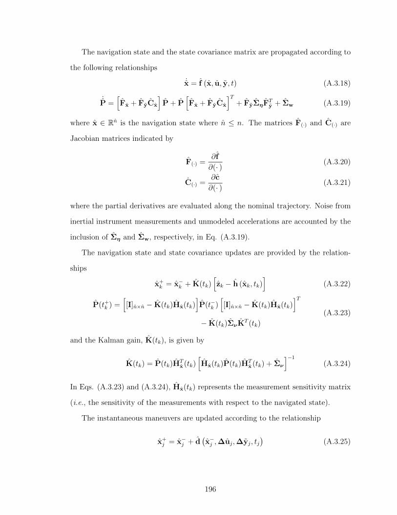
The navigation state and the state covariance matrix are propagated according to
the following relationships
˙x = f (x, u, y, t) (A.3.18)
˙P =
[Fx + FyCx
]P + P
[Fx + FyCx
]T+ FyΣηF
Ty + Σw (A.3.19)
where x ∈ Rn is the navigation state where n ≤ n. The matrices F(·) and C(·) are
Jacobian matrices indicated by
F(·) =∂ f
∂(· )(A.3.20)
C(·) =∂c
∂(· )(A.3.21)
where the partial derivatives are evaluated along the nominal trajectory. Noise from
inertial instrument measurements and unmodeled accelerations are accounted by the
inclusion of Ση and Σw, respectively, in Eq. (A.3.19).
The navigation state and state covariance updates are provided by the relation-
ships
x+k = x−k + K(tk)
[zk − h (xk, tk)
](A.3.22)
P(t+k ) =[[I]n×n − K(tk)Hx(tk)
]P(t−k )
[[I]n×n − K(tk)Hx(tk)
]T− K(tk)ΣνK
T (tk)
(A.3.23)
and the Kalman gain, K(tk), is given by
K(tk) = P(tk)HTx (tk)
[Hx(tk)P(tk)H
Tx (tk) + Σν
]−1
(A.3.24)
In Eqs. (A.3.23) and (A.3.24), Hx(tk) represents the measurement sensitivity matrix
(i.e., the sensitivity of the measurements with respect to the navigated state).
The instantaneous maneuvers are updated according to the relationship
x+j = x−j + d
(x−j ,∆uj,∆yj, tj
)(A.3.25)
196
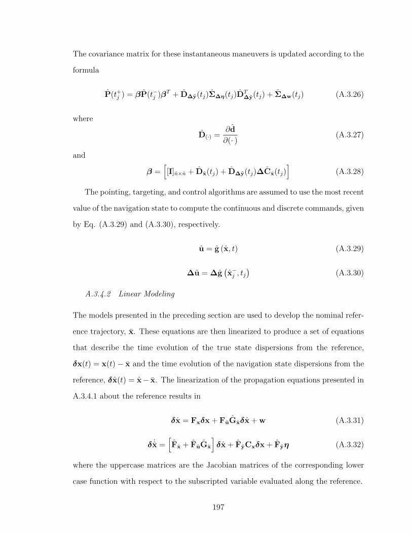
The covariance matrix for these instantaneous maneuvers is updated according to the
formula
P(t+j ) = βP(t−j )βT + D∆y(tj)Σ∆η(tj)DT∆y(tj) + Σ∆w(tj) (A.3.26)
where
D(·) =∂d
∂(· )(A.3.27)
and
β =[[I]n×n + Dx(tj) + D∆y(tj)∆Cx(tj)
](A.3.28)
The pointing, targeting, and control algorithms are assumed to use the most recent
value of the navigation state to compute the continuous and discrete commands, given
by Eq. (A.3.29) and (A.3.30), respectively.
u = g (x, t) (A.3.29)
∆u = ∆g(x−j , tj
)(A.3.30)
A.3.4.2 Linear Modeling
The models presented in the preceding section are used to develop the nominal refer-
ence trajectory, x. These equations are then linearized to produce a set of equations
that describe the time evolution of the true state dispersions from the reference,
δx(t) = x(t)− x and the time evolution of the navigation state dispersions from the
reference, δx(t) = x− x. The linearization of the propagation equations presented in
A.3.4.1 about the reference results in
δx = Fxδx + FuGxδx + w (A.3.31)
δ ˙x =[Fx + FuGx
]δx + FyCxδx + Fyη (A.3.32)
where the uppercase matrices are the Jacobian matrices of the corresponding lower
case function with respect to the subscripted variable evaluated along the reference.
197
The state updates can also be linearized about the reference, which results in the
relationships
δx+k = δx−k (A.3.33)
δx+k = K(tk)Hx(tk)δx
−k +
[[I]− K(tk)Hx(tk)
]δx−k + K(tk)νk (A.3.34)
The state corrections for impulsive maneuvers are given by
δx+j = [[I] + Dx(tj)] δx
−j + D∆u(tj)∆Gx(tj)δx
−j + ∆wj (A.3.35)
δx+j =
[[I] + Dx(tj) + D∆u(tj)∆Gx(tj)
]δx−j
+ D∆y(tj)δ∆Cx(tj)x−j + D∆y(tj)∆ηj
(A.3.36)
where again the uppercase matrices are the Jacobian matrices of the correspond-
ing lower case function with respect to the subscripted variable evaluated along the
reference.
An augmented state vector, x = (δx δx)T , consisting of both the true state dis-
persions (δx) and the navigation state dispersions (δx) can be created. The linearized
equations described in Eqs. (A.3.31)-(A.3.36) reduce to the matrix form
x = Fx + Gη + Ww (A.3.37)
x+k = A(tk)x
−k + B(tk)νk (A.3.38)
x+j = D(tj)x
−k + M(tj)∆ηj + N (tj)∆wj (A.3.39)
where the matrices are given by
F =
Fx FuGx
FyCx Fx + FuGx
, G =
[0]n×ny
Fy
, W =
[I]n×n
[0]n×n
(A.3.40)
A(tk) =
[I]n×n [0]n×n
K(tk)Hx(tk) [I]n×n − K(tk)Hx
, B(tk) =
[0]n×ny
K(tk)
(A.3.41)
D(tj) =
[I]n×n + Dx(tj) D∆u(tj)∆Gx(tj)
D∆y(tj)∆Cx(tj) [I]n×n + Dx(tj) + D∆u(tj)∆Gx(tj)
(A.3.42)
198
M(tj) =
[0]n×n∆y
D∆y(tj)
, N (tj) =
[I]n×n
[0]n×n
(A.3.43)
A.3.5 Covariance Equations
The equations governing the propagation, update, and maneuver correction for the
augmented state vector’s, x, covariance matrix ΣA = E[xxT ] are formulated as follows
ΣA = FΣA + ΣAFT + GTΣηG + WΣwWT (A.3.44)
ΣA(t+k ) = A(t−k )ΣA(t−k )AT (t−k ) + B(t−k )Σν(t−k )BT (t−k ) (A.3.45)
ΣA(t+j ) = D(t−j )ΣA(t−j )DT (t−j )+M(t−j )Σ∆η(t−j )MT (t−j )
+ N (t−j )Σ∆w(t−j )N T (t−j )
(A.3.46)
Where it is noted that since E[x(t)] = E[x(t)] and E[x(t)] = E[x(t)], E[x] = 0.
Furthermore, it is assumed that w, ∆w, η, ∆ηj, and νk are mutually uncorrelated.
Along with Eqs. (A.3.19), (A.3.23), (A.3.24), and (A.3.26), Eqs.(A.3.44) - (A.3.46)
represents a complete set of linear covariance analysis equations.
A.3.5.1 Dispersion Analysis
The closed-loop GN&C system can be evaluated based upon the true state dispersions,
D, the navigation state dispersion D, and the covariance of the true navigation state
errors, P. The are given by
D = E[δx(t)δxT (t)] = [[I]n×n [0]n×n] ΣA [[I]n×n [0]n×n]T (A.3.47)
D = E[δx(t)δxT (t)] = [[0]n×n [I]n×n] ΣA [[0]n×n [I]n×n]T (A.3.48)
P = E[(δx(t)−Mxδx)(δx(t)−Mxδx)T ]
= [−Mx [I]n×n] ΣA [−Mx [I]n×n]T(A.3.49)
where it is assumed that the true navigation states are mapped from the states by a
function of the form
xn = m(x) (A.3.50)
199
and Mx = ∂m/∂x. With these performance measures in place, P can be compared
to P to evaluate the onboard navigation performance, and the ability of the GN&C
system to control trajectory errors can be examined by evaluating D.
A.4 Proof of Lyapunov’s Direct Method
The following proof for Lyapunov’s direct method follows that outlined in Refs. [142]
and [143].
Proof: Lyapunov’s Direct Method for Discrete Dynamical Systems. Choose r0 > 0 such
that yk : ‖ yk − ye ‖≤ r0 ⊂ S ∩ D. By the continuity of f there is an r1 ≤ r0
such that ‖ f(yk) − ye ‖≤ r0 whenever ‖ yk − ye ‖≤ r1. Now let ε > 0 be given
and assume, without loss of generality, that ε ≤ r1. Then choose δ ∈ (0, ε) so that
‖ yk − ye ‖≤ δ implies that
V (yk) < φ(ε) ≡ minV (yk) : ε ≤‖ yk − ye ‖≤ r0
This can be achieved using the continuity of V and the fact that V (yk) is positive
definite. Now suppose there is some y0 such that ‖ y0−ye ‖≤ δ but ‖ yk+1−ye ‖> ε
for some k. Assume that this is the first such k; thus ‖ yi − ye ‖≤ ε ≤ r1, i =
1, 2, · · · , k. Then ‖ f(yk)− ye ‖≤ r0 so that V (f(yk)) is well-defined and V (f(yk)) ≥
φ(ε). But by the definition of a Lyapunov function
V (yk+1) ≤ V (yk) ≤ · · · ≤ V (y0) < φ(ε)
This is a contradiction and stability is proved.
For asymptotic stability, it suffices to consider any sequence yk ⊂ yk : ‖
yk − ye ‖≤ ε and show that yk → ye as k →∞, and for this it suffices to show that
if y is any limit point of yk, then y = ye. Suppose not, then the mapping
r(yk) =V (f(yk))
V (yk)
200
is well-defined and continuous in some open neighborhood S0 of y and since ∆V < 0,
r(y) < 1. Hence, for a given α ∈ (r(y), 1), there is a δ > 0 such that r(yk) ≤
α whenever ‖ yk − y ‖≤ δ. Therefore, for sufficiently large ki, the subsequence
converging to y satisfies
V (yki+1) = V (f(yki+1)) ≤ αV (yki) ≤ · · · ≤ αV (yki−1+1) ≤ · · · ≤ αiV (y0)
so that V (yki) → 0 as i → ∞. But the continuity of V implies that V (y) = 0,
and because the Lyapunov function is positive definite, y = ye proving asymptotic
stability.
For global asymptotic stability, note that for any y0, the radial unboundedness
of the Lyapunov function guarantees that yk is bounded otherwise there would be
a subsequence yki such that ‖ yki − ye ‖→ ∞ as i → ∞ and hence V (yki) → ∞
as i → ∞. This contradicts the monotone decreasing behavior of V (yk) required by
∆V < 0. It now follows precisely as in the case of asymptotic stability that yk → ye
as k →∞ proving global asymptotic stability.
A.5 Proof of Uniform (Exponential) Stability Criterion
The following proofs are adapted from Ref. [150].
A.5.1 Linear Systems
Proof: Uniform (Exponential) Stability for Linear Systems. The positive definite de-
crescent function Vk , ‖Wkyk ‖ satisifes
∆Vk = ‖Wk+1Akyk ‖ − ‖Wkyk ‖ ≤ −(1− β) ‖Wkyk ‖ < 0
which implies uniform (exponential) asymptotic stability by Lyapunov’s direct method
proven by Hahn in Ref. [142].
201
A.5.2 Nonlinear Systems
Proof: Uniform (Exponential) Stability for Nonlinear Systems. For any y ∈ Ω, the
fundamental theorem of calculus gives
f(k,y) = f(k,y)− f(k,0) =
[∫ 1
0
∂f
∂y(k, λy)dλ
]y
Consider the positive definite decrescent function V (y) , ‖Wy ‖. Since Ω is open
with 0 ∈ Ω, ds , supd
[y | V (y ≤ d ⊂ Ω] > 0. Define Xs , y | V (y) < ds ⊂ Ω
which is open and 0 ∈ Xs. Then, for any k ≥ 0, if yk ∈ Xs
∆Vk = ‖Wyk+1 ‖ − ‖Wyk ‖
= ‖∫ 1
0
W
[∫ 1
0
∂f
∂y(k, λy)
]ykdλ ‖ − ‖Wyk ‖
≤ −(1− β) ‖Wyk ‖< 0
which implies that yk+1 ∈ Xs. By induction if y0 ∈ Xs, yk ∈ Xs and ∆Vk < 0 ∀k ≥ 0.
Given y0 ∈ Xs, choose β0 such that
supk
supv∈X0
nW
[∂f
∂y(v)
]W−1
n≤ β0 ≤ β < 1
where X0 , y | V (y) ≤ V (y0). Then ∆Vk < −(1 − β0)Vk and the exponential
bounds follows from Lemma 1 with M = 0, α = (1− β0), and c =‖W−1 ‖−1.
A.6 Proof of Region of Attraction
This proof follows that outlined in Ref. [145]
Proof: Region of Attraction. If y0 ∈ A0 then the third condition on w(y) shows that
w(y1) ≤ w(y0) so that y1 ∈ A0 and, by induction, yk ∈ A0 and w(yk+1) ≤ w(yk), k =
2, · · · . Hence the sequence w(yk) converges. Also note that the third condition on
w(y) implies that
1− w(f(y))
1− w(y)= 1 + φ(y), y ∈ A0
202
so that
1− w(yk)
1− w(y0)=
k−1∏i=0
1− w(yi+1)
1− w(yi)=
k−1∏i=0
1 + φ(yi)
Since the left hand side of this equality converges as k → ∞, the right does as well
which implies that φ(yk) → 0 as k → ∞. Then the first condition on w(y) and the
continuity of φ ensures that yk → ye as k → ∞. Conversely, suppose that y0 /∈ A0
then the third condition on w(y) shows that w(y1) ≥ w(y0) ≥ 1 so that y1 /∈ A0 and,
by induction, w(yk) ≥ 1, k = 2, 3, · · · . But if limk→∞
yk = ye, then the continuity of w
requires that limk→∞
w(yk) = 0 which is a contradiction.
203
APPENDIX B
PUBLICATIONS
B.1 Journal Articles
B.1.1 Published Journal Articles
• Other articles:
1. Steinfeldt, B.A., Grant, M.J., Matz, D.A., Braun, R.D., and Barton, G.,“Guidance Navigation and Control System Performance Trades for MarsPinpoint Landing,” Journal of Spacecraft and Rockets, Vol. 47, No. 1, pp.188-198, Jan-Feb, 2010.
2. Grant, M.J., Steinfeldt, B.A., Braun, R.D., and Barton, G.H., “SmartDivert: A New Entry, Descent and Landing Architecture,” Journal ofSpacecraft and Rockets, Vol. 47, No. 3, pp. 385-393, May-June, 2010.
B.1.2 Pending Journal Articles
• Thesis relevant articles:
1. Steinfeldt, B.A. and Braun, R.D., “Use of Dynamical System Theory inMultidisciplinary Design”
An article describing how to cast the multidisciplinary design problemas a dynamical system theory with an overview of potential applicationdomains based on “Utilizing Dynamical Systems Concepts in Multidisci-plinary Design”; submitted to the AIAA Journal in November 2012 (inrevision; recommended for publication).
2. Steinfeldt, B.A., Rossman, G.A., Braun, R.D., and Barton, G.H., “RapidRobust Design of a Deployable for Strategic Systems”
An article based on “Rapid Robust Design of a Deployable System forBoost-Glide Vehicles” where the complete design of the two mid L/D sys-tems are found using the rapid robust design methodology; submitted tothe Journal of Spacecraft and Rockets in May 2013.
204
B.1.3 Planned Journal Articles
• Thesis relevant articles:
1. Steinfeldt, B.A. and Braun, R.D., “Multidisciplinary Design Conver-gence Criterion Based on Stability Concepts”
An article describing the convergence criterion derived through stabilityconcepts for various root-finding schemes that is based on “Design Con-vergence Using Stability Concepts from Dynamical Systems Theory”; tar-geted for submission to Engineering Optimization in Fall 2013.
2. Steinfeldt, B.A. and Braun, R.D., “Using Optimal Control to Incorpo-rate Design Constraints in the Multidisciplinary Design Problem”
An article describing the use of optimal control techniques to incorpo-rate constraints within the multidisciplinary design problem that is basedon “Leveraging Dynamical Systems Theory to Incorporate Design Con-straints for Multidisciplinary Design Problems”; targeted for submissionto the ASME Journal of Mechanical Design in Fall 2013.
3. Steinfeldt, B.A. and Braun, R.D., “Leveraging Estimation Techniquesin Multidisciplinary Design”
An article describing the use of estimation techniques to quantify uncer-tainty within the multidisciplinary design problem that is based on “UsingEstimation Techniques in Multidisciplinary Design”; targeted for submis-sion to Engineering Optimization in Fall 2013.
4. Steinfeldt, B.A. and Braun, R.D., “Extensibility of a Linear Rapid Ro-bust Design Methodology”
An article demonstrating the linear robust design methodology appliedto nonlinear designs and the extent to which it is appropriate that is basedon “Extensibility of a Linear Rapid Robust Design Methodology”; targetedfor submission to the AIAA Journal in Fall 2013.
B.2 Conference Papers
B.2.1 Published Conference Papers
• Thesis relevant conference papers:
1. Steinfeldt, B.A., Theisinger, J.E., Korzun, A.M., Clark, I.G., Grant,M.J., and Braun, R.D., “High Mass Mars Entry, Descent and Landing Ar-chitecture Assessment,” AIAA-2009-6684, AIAA SPACE 2009 Conferenceand Exposition, September 2009, Pasadena, California.
205
2. Steinfeldt, B.A., Braun, R.D., and Paschall, S.C., “Guidance and Con-trol Algorithm Robustness Baseline Indexing,” AIAA-2010-8827, AIAAGuidance, Navigation and Control Conference, August 2010, Toronto, On-tario, Canada.
3. Steinfeldt, B.A. and Braun, R.D., “Utilizing Dynamical Systems Con-cepts in Multidisciplinary Design,” AIAA-2012-5655, AIAA/ISSMO Mul-tidisciplinary Analysis and Optimization Conference, September 2012, In-dianapolis, Indiana.
4. Steinfeldt, B.A. and Braun, R.D., “Design Convergence Using StabilityConcepts from Dynamical Systems Theory,” AIAA-2012-5657, AIAA/ISSMOMultidisciplinary Analysis and Optimization Conference, September 2012,Indianapolis, Indiana.
5. Steinfeldt, B.A., Rossman, G.A., and Braun, R.D., “Rapid Robust De-sign of a Deployable System for Boost-Glide Vehicles,” AIAA-2013-0031,51st AIAA Aerospace Sciences Meeting including the New Horizons Forumand Aerospace Exposition, January 2013, Grapevine, Texas.
6. Steinfeldt, B.A. and Braun, R.D., “Leveraging Dynamical Systems The-ory to Incorporate Design Constraints for Multidisciplinary Design Prob-lems,” AIAA-2013-1041, 51st AIAA Aerospace Sciences Meeting includ-ing the New Horizons Forum and Aerospace Exposition, January 2013,Grapevine, Texas.
• Other conference papers:
1. Thompson, R., Cliatt, L., Gruber, C., Steinfeldt, B., Sebastian, T., andWilson, J., “Design of an Entry System for Cargo Delivery to Mars,” 5thInternational Planetary Probe Workshop, June 2007, Bordeaux, France.
2. Otero, R.E., Grant, M.J., Steinfeldt, B.A., and Braun, R.D., “Introduc-ing PESST: A Conceptual Design and Analysis Tool for Unguided/GuidedEDL Systems,” 6th International Planetary Probe Workshop, June 2008,Atlanta, Georgia.
3. Steinfeldt, B.A., Grant, M.J., Matz, D.A., Braun, R.D., and Barton,G.H., “Guidance, Navigation, and Control Technology System Trades forMars Pinpoint Landing,” AIAA-2008-6216, AIAA Atmospheric Flight Me-chanics Conference, August 2008, Honolulu, Hawaii.
4. Grant, M.J, Steinfeldt, B.A., Braun, R.D, and Barton, G.H., “SmartDivert: A New Entry, Descent, and Landing Architecture,” AIAA 2009-0522, 47th AIAA Aerospace Sciences Meeting Including the New HorizonsForum and Aerospace Exposition, January 2009, Orlando, Florida.
5. Steinfeldt, B.A., and Tsiotras, P., “A State-Dependent Riccati Equa-tion Approach to Atmospheric Entry Guidance,” AIAA-2010-8310, AIAAGuidance, Navigation and Control Conference, August 2010, Toronto, On-tario, Canada.
206

6. Chua, Z. K., Steinfeldt, B.A., Kelly, J. R., and Clark I.G., “SystemLevel Impact of Landing Point Redesignation for High-Mass Mars Mis-sions,” AIAA-2011-7296, AIAA SPACE 2011 Conference and Exposition,September 2011, Long Beach, California.
7. Cruz-Ayoroa, J.G., Kazemba, C.D., Steinfeldt, B.A., Kelly, J.R., Clark,I.G., and Braun, R.D., “Mass Model Development for Conceptual Design ofa Hypersonic Rigid Deployable Decelerator,” 9th International PlanetaryProbe Workshop, June 2012, Toulouse, France.
8. Miller, M.J., Steinfeldt, B.A., and Braun, R.D., “Mission ArchitectureConsiderations for Recovery of High-Altitude Atmospheric Dust Samples,”accepted for presentation at the 2013 AIAA Atmospheric Flight MechanicsConference, Boston, MA, August 2013.
9. Braun, R.D., Putnam, Z.R., Steinfeldt, B.A., Grant, M.J., and Bar-ton, G.H., “Guidance Development for Aerospace Systems,” accepted forpresentation at the 2013 AIAA Guidance, Navigation, and Control Con-ference, Boston, MA, August 2013. (Invited)
B.2.2 Planned Conference Papers
• Thesis relevant conference papers:
1. Steinfeldt, B.A. and Braun, R.D., “Using Estimation Techniques in Mul-tidisciplinary Design”
Paper describing the use of the Kalman filter in multidisciplinary design toquantify uncertainty; submitted to SciTech 2014. (January 13-17, 2014)
2. Steinfeldt, B.A. and Braun, R.D., “Extensibility of a Linear Rapid Ro-bust Design Methodology”
Paper demonstrating the linear robust design methodology applied to non-linear designs and the extent to which it is appropriate; submitted toSciTech 2014. (January 13-17, 2014)
• Other conference papers:
1. Miller, M.J, Steinfeldt, B.A., and Braun, R.D., “Supersonic InflatableAerodynamic Decelerators for use on Sounding Rocket Payloads,” submit-ted to SciTech 2014. (January 13-17, 2014)
207

REFERENCES
[1] Accreditation Board for Engineering and Technology, Baltimore, Maryland,Criteria for Accrediting Engineering Programs: Effective for Evaluations Duringthe 2009-2010 Accreditation Cycle, Dec. 2008.
[2] Ackoff, R. L., Redesigning the Future: A Systems Approach to Societal Prob-lems , John Wiley & Sons, Inc., New York, NY, 1974.
[3] Carlock, P. G., Decker, S. C., and Fenton, R. E., “Agency Level Systems Engi-neering for Systems of Systems,” Systems and Information Technology ReviewJournal , 1999.
[4] Carlock, P. G. and Fenton, R. E., “Systems of Systems (SoS) Enterprise Sys-tems Engineering for Information-Intensive Organizations,” Systems Engineer-ing , Vol. 4, No. 4, 2001.
[5] Kotov, V., Rokicki, T. M., and Cherkasova, L., “CSL: Communicating Struc-tures Library for Systems Modeling and Analysis,” Tech. Rep. HPL-98-118, HPLaboratories, 1998.
[6] Pei, R. S., “Systems of Systems Integration (SoSI)-A Smart Way of Acquir-ing Army C4I2WS Systems,” Proceedings of the Summer Computer SimulationConference, San Diego, CA, July 2000.
[7] Lukasik, S. J., “Systems, systems of systems, and the education of engi-neers,” Artificial Intellience for Engineering Design, Analysis and Manufac-turing , Vol. 12, No. 1, 1998.
[8] William H. J. Manthorpe, J., “The Emerging Joint System of Systems: ASystems Engineering Challenge and Opportunity for APL,” John Hopkins APLTechnical Digest , Vol. 17, No. 3, 1996.
[9] Held, J. M., Systems of Systems: Principles, Performance, and Modelling ,Ph.D. thesis, The University of Sydney, Sydney, NSW, Feb. 2008.
[10] Jamshidi, M., Systems of Systems Engineering: Innovations for the 21st Cen-tury , John Wiley & Sons, Inc., Hoboken, NJ, 2008.
[11] Gebala, D. A. and Eppinger, S. D., “Methods for Analyzing Design Procedures,”Design Theory and Methodology , Vol. 31, 1991, pp. 228–233.
[12] Alexander, C., Notes on the Synthesis of Form, Harvard University Press, 1964.
[13] Simon, H. A., The Sciences of the Artificial , MIT Press, 1970.
208
[14] Sobieszczanski-Sobieski, J., “Multidisciplinary Optimization for EngineeringSystems: Achievements and Potential,” Tech. Rep. TM-101566, NASA, 1989.
[15] Harary, F., Graph Theory , Addison-Wesley, 1969.
[16] Wiest, J. D. and Levy, F. K., A Management Guide to PERT/CPM , Prentice-Hall, 1977.
[17] Steward, D. V., “The Design Structure System: A Method for Managing theDesign of Complex Systems,” IEEE Transactions on Engineering Management ,Vol. 28, 1981, pp. 71–74.
[18] Young, D. A., An Innovative Method for Allocating Reliability and Cost in aLunar Exploration Architecture, Ph.D. thesis, Georgia Institute of Technology,Georgia, May 2007.
[19] McCord, K. R., Managing the Integration Problem in Concurrent Engineering ,Master’s thesis, Massachusetts Institute of Technology, Massachusetts, May1993.
[20] Berkes, U. L., “Efficient Optimization of Aircraft Structures with a Large Num-ber of Design Variables,” Journal of Aircraft , Vol. 27, No. 12, 1990.
[21] Martins, J. R. R. A. and Lambe, A. B., “Multidisciplineary Design Optimiza-tion: A Survey of Architectures,” AIAA Journal (in press).
[22] Sobieszczaanski-Sobieski, J. and Haftka, R. T., “Multidisciplinary AerospaceDesign Optimization - Survey of Recent Developments,” 34th AIAA AerospaceSciences Meeting and Exhibit , Reno, NV, Jan. 1996.
[23] Hajela, P., Bloebaum, C. L., and Sobieszczanski-Sobieski, J., “Application ofGlobal Sensitivity Equations in Multidisciplinary Aircraft Synthesis,” Journalof Aircraft , Vol. 27, No. 12, 1990.
[24] Sobieszczanski-Sobieski, J., “Sensitivity Analysis and Multidisciplinary Opti-mization for Aircraft Design: Recent Advances and Results,” Journal of Air-craft , Vol. 27, No. 12, 1990.
[25] Sobieszczanski-Sobieski, J., “A System Approach to Aircraft Optimization,”Tech. Rep. TM-104074, NASA, March 1991.
[26] Sobieszczanski-Sobieski, J., “Sensitivity of Complex, Internally Coupled Sys-tems,” AIAA Journal , Vol. 28, No. 1, 1990.
[27] Olds, J. R., “System Sensitivity Analysis Applied to the Conceptual Design ofa Dual Fuel Rocket SSTO,” 5th AIAA/NASA/USAF/ISSMO Symposium onMultidisciplinary Analysis and Optimization, Panama City Beach, FL, Sept.1994.
209
[28] McCormick, D. J., Distributed Uncertainty Analysis Techniques for ConceptualLaunch Vehicle Design, Ph.D. thesis, Georgia Institute of Technology, Georgia,July 2001.
[29] Rogers, J. L., “A Design Manger’s Aid for Intelligent Decomposition–User’sGuide,” Tech. Rep. TM-101575, NASA, March 1989.
[30] Otero, R. E., Problem Decomposition by Mutual Information and Force-BasedClustering , Ph.D. thesis, Georgia Institute of Technology, Georgia, May 2012.
[31] Ledsinger, L., Solutions to Decomposed Branching Trajectories with PoweredFlyback Using Multidisciplinary Design Optimization, Ph.D. thesis, GeorgiaInstitute of Technology, Georgia, July 2000.
[32] Balling, R. J. and Sobieszczanski-Sobieski, J., “An Algorithm for Solving theSystem-Level Problem in Multilevel Optimization,” Tech. Rep. CR-195015,NASA, Dec. 1994.
[33] Braun, R. D., Collaborative Optimization: An Architecture for Large-Scale Dis-tributed Design, Ph.D. thesis, Stanford University, Stanford, CA, May 1995.
[34] Cormier, T. A., Scott, A., Ledsinger, L. A., McCormick, D. J., Way, D., andOlds, J. R., “Comparision of Collaborative Optimization to Conventional De-sign Techniques for a Conceptual RLV,” AIAA 2000-4885 , Long Beach, CA,Sept. 2000.
[35] Braun, R. D. and Kroo, I. M., “Development and Application of the Collabo-rative Optimization Architecture in a Multidisciplinary Design Environment,”International Congress on Industrial and Applied Mathematics , Aug. 1995.
[36] Budianto, I. A., A Collaborative Optimization Approach to Inprove the Designand Deployment of Satellite Constellations , Ph.D. thesis, Georgia Institute ofTechnology, Georgia, Sept. 2000.
[37] Braun, R. D., Gage, P., Kroo, I. M., and Sobieski, I., “Implementation andPerformance Issues in Collaborative Optimization,” AIAA 96-4017 , Bellevue,WA, Sept. 1996.
[38] Braun, R. D., Kroo, I. M., and Moore, A., “Use of the Collaborative Optimiza-tion Architecture for Launch Vehicle Design,” AIAA 96-4018 , Bellevue, WA,Sept. 1996.
[39] “Merriam-Webster,” Nov 2011.
[40] Mavris, D. N., Bandte, O., and Schrage, D. P., “Application of ProbabilisticMethods for the Determination of an Economically Robust HSCT Configura-tion,” AIAA 1996-4090 , Bellevue, WA, Sept. 1996.
210
[41] DeLaurentis, D. A., A Probabilistic Approach to Aircraft Design EmphasizingStability and Control Uncertainties , Ph.D. thesis, Georgia Institute of Technol-ogy, Atlanta, GA, Nov. 1998.
[42] Zhao, K., Glover, K., and Doyle, J. C., Robust and Optimal Control , PrenticeHall, Englewood Cliffs, NJ, 1996.
[43] Hazelrigg, G. A., Systems Engineering: An Approach to Information-BasedDesign, Prentice Hall, Upper Saddle Ridge, NJ, 1996.
[44] Siddall, J. N., Probabilistic Engineering Design, Marcel Dekker, Inc., 1983.
[45] Mavris, D. N., Bandte, O., and DeLaurentis, D. A., “Robust Design Simulation:A Probabilistic Approach to Multidisciplinary Design,” Journal of Aircraft ,Vol. 36, No. 1, 1999.
[46] Yen, B. and Tung, Y., Reliability and Uncertainty Analyses in Hydraulic Design,American Society of Chemical Engineers, New York, NY, 1993.
[47] McCormick, D. J. and Olds, J. R., “System Robustness Comparison of Ad-vanced Space Launch Concepts,” AIAA 98-5209 , Huntsville, AL, Oct. 1998.
[48] DeLaurentis, D. A. and Mavris, D. N., “Uncertainty Modeling and Managementin Multidisciplinary Analysis and Synthesis,” AIAA 2000-0422 , Reno, NV, Jan.2000.
[49] DeLaurentis, D. A., Mavris, D. N., Calise, A. C., and Schrage, D. P., “Gen-erating Dynamic Models Including Uncertainty for Use in Aircraft ConceptualDesign,” AIAA 97-3590 , New Orleans, LA, Aug. 1997.
[50] Mavris, D. N., DeLaurentis, D. A., and Soban, D. S., “Probabilistic Assessmentof Handling Qualities Constraints in Aircraft Preliminary Design,” AIAA 98-0492 , Reno, NV, Jan. 1998.
[51] Mavris, D. N., DeLaurentis, D. A., Bandte, O., and Hale, M. A., “A StochasticApproach to Multi-disciplinary Aircraft Analysis and Design,” AIAA 98-0912 ,Reno, NV, Jan. 1998.
[52] Mavris, D. N., Bandte, O., and Schrage, D. P., “Effect of Mission Requirementson the Economic Robustness of an HSCT Concept,” Proceedings of the 18thAnnual Conference of the International Society of Parametric Analysts , Cannes,France, June 1996.
[53] Mavris, D. N., Bandte, O., and DeLaurentis, D. A., “Determination of SystemFeasibility and Viability Employing a Joint Probabilistic Formulation,” AIAA99-0183 , Reno, NV, Jan. 1999.
[54] Mavris, D. N. and Bandte, O., “A Probabilistic Approach to UCAV EngineSizing,” AIAA 98-3264 , Anaheim, CA, July 1998.
211
[55] Roth, B. A., Mavris, D. N., and Elliott, D., “A Probabilistic Approach to Mul-tivariate Constrained Robust Design Simulation,” AIAA 98-3264 , Cleveland,OH, July 1998.
[56] Mavris, D. N. and Bandte, O., “Comparison of Two Probabilistic Techniquesfor the Assessment of Economic Uncertainty,” Proceedings of the 19th AnnualConference of the International Society of Parametric Analysts , New Orleans,LA, May 1997.
[57] Lafleur, J. M., “Trading Robustness Requirements in Mars Entry TrajectoryDesign,” AIAA 2009-561 , Chicago, IL, Aug. 2009.
[58] Vysocanskii, D. and Petunin, J., “Justification of the 3σ Rule for UnimodalDistributions,” Theory of Probability and Mathematical Statistics , Vol. 21, 1980,pp. 25–36.
[59] Hogg, R. V. and Tanis, E. A., Probability and Statistical Inference, PearsonPrentice Hall, Upper Saddle River, NJ, 2006.
[60] Roos, O. V., “A Formal Solution of Liouville’s Equation,” Tech. Rep. 32-10,Jet Propulsion Laboratory, March 1960.
[61] Fuller, A. T., “Analysis of Nonlinear Stochastic Systems by Means of theFokker-Planck Equation,” International Journal of Control , Vol. 9, No. 6, 1969.
[62] Risken, H., The Fokker-Planck Equation: Methods of Solution and Applications ,Springer, New York, NY, 1996.
[63] Kalos, M. H. and Whitlock, P. A., Monte Carlo Methods , Wiley-VCH, 2008.
[64] Chen, W., Allen, J. K., Schrage, D. P., and Mistree, F., “Statistical Experimen-tation Methods for Achieving Affordable Concurrent Systems Design,” AIAAJournal , Vol. 35, No. 5, 1997.
[65] Unal, R., Stanley, D., Engelund, W., and Lepsch, R., “Design for Quality Us-ing Response Surface Methods: An Alternative to Taguchi’s Parameter DesignApproach,” Engineering Management Journal , Vol. 6, No. 3, 1994.
[66] Klenijen, J. P., Statistical Tools for Simulation Practitioners , Marcel Dekker,New York, NY, 1987.
[67] Chen, W., Tsui, K.-L., Allen, J. K., and Mistree, F., “Integration of ResponseSurface Method with the Compromise Decision Support Problem in Developinga General Robust Design Procedure,” Advances in Design Automation, Vol. 82,No. 2, 1995.
[68] Mavris, D. N. and Bandte, O., “Economic Uncertainty Assessment Using aCombined Design of Experiments/Monte Carlo Simulation Approach with Ap-plication to an HSCT,” 17th Annual Conference of the International Society ofParametric Analysts , San Diego, CA, May 1995.
212
[69] Madsen, H. O., Krenk, S., and Lind, N. C., Methods of Structural Safety , Pren-tice Hall, Englewood Cliffs, NJ, 1986.
[70] Wu, Y. T., “Structural Reliability Analysis Methods for Implicit PerformanceFunctions,” Proceedings of the ASCE Special Conference in Probabilistic Me-chanics and Structural and Geotechnical Reliability , New York, NY, 1992.
[71] Khalessi, M. R., Wu, Y. T., and Torng, T. Y., “Most-Probable-Point-LocusReliability Method in Standard Normal Space,” ASME Design Engineering ,Vol. 30, 1991.
[72] Wirshing, P. H. and Martin, W. S., “Fracture Mechanics Fatigue ReliabilityAssessment Employing the Most Probable Point Locus Method,” Proceedingsof the the 5th ASCE Special Conference in Probabilistic Methods in Civil Engi-neering , New York, NY, 1988.
[73] Wu, Y. T., Millwater, H. R., and Cruse, T. A., “An Advanced ProbabilisticStructural Analysis Method for Implicit Performance Functions,” AIAA Jour-nal , Vol. 28, No. 9, 1990.
[74] Liu, W. K. and Belytschko, T., Computational Mechanics of Reliability Analy-sis , Elmepress International, Lauseanne, WA, 1989.
[75] Wu, Y. T. and Wirsching, P. H., “Demonstration of a Fast, New ProbabilityIntegration Method for Reliability Analysis,” ASME Journal of Engineering forIndustry , Vol. 109, 1987.
[76] Wu, Y. T. and Wirsching, P. H., “Advanced Reliability Methods for Proba-bilistic Structural Analysis,” ASCE Structural Safety and Reliability , Vol. 3,1989.
[77] Wu, Y. T. and Wirsching, P. H., “New Algorithm for Structural ReliabilityEstimation,” ASCE Journal of Engineering Mechanics , Vol. 113, No. 9, 1987.
[78] Southwest Reserach Institute, San Antonio, TX, FPI User’s Manual and The-oretical Manual , 1995.
[79] Du, X. and Chen, W., “A Most Probable Point Based Method for UncertaintyAnalysis,” Journal of Design and Manufacturing Automation, Vol. 4, 2001.
[80] Mahadevan, S. and Cruse, T. A., “Advanced First-Order Method for SystemReliability,” Proceedings of the the ASCE Special Conference in ProbabilisticMechanics and Geotechnical Reliability , New York, NY, 1992.
[81] Lin, H. Z. and Khalessi, M. R., “Calculation of Failure Probability by UsingX-Space Most-Probable-Point,” AIAA 93-1624 , La Jolla, CA, 1993.
[82] Geller, D. K., “Linear Covariance Techniques for Orbial Rendezvous Analysisand Autonomous Onboard Mission Planning,” Journal of Guidance, Control,and Dynamics , Vol. 29, No. 6, 2006, pp. 1404–1414.
213
[83] Christensen, D. and Geller, D., “Terrain-Relative and Beacon-Relative Navi-gation for Lunar Powered Descent and Landing,” AAS 009-057 , Breckenridge,CO, Jan. 2009.
[84] Geller, D. K. and Christensen, D. P., “Linear Covariance Analysis for PoweredLunar Descent and Landing,” Journal of Spacecraft and Rockets , Vol. 46, No. 6,2009.
[85] Du, X. and Chen, W., “Methodolgoy for Managing the Effect of Uncertainty inSimulation-Based Design,” AIAA Journal , Vol. 38, No. 8, 2000.
[86] Kawata, T., “Fourier Analysis in Probability Theory,” Probability and Mathe-matical Statistics, A Series of Monographs and Textbooks , Vol. 55, No. 3, 1975.
[87] Hoybye, J. A., “Model Error Propagation and Data Collection Design: An Ap-plication in Water Quality Modeling,” Water, Air, and Soil Pollution, Vol. 103,No. 1, 1998.
[88] Isukapalli, S. S. and Georgopoulos, P. G., “Stochastic Response Surface Meth-ods (SRSMs) for Uncertainty Propagation: Application to Environmental andBiological Systems,” Risk Analysis , Vol. 18, No. 3, 1998.
[89] Cheng, W., Parametric Uncertainty Analysis for Complex Engineering Systems ,Ph.D. thesis, Massachusetts Institute of Technology, Massachussetts, June 1999.
[90] Kumar, M., Singla, P., Chakravorty, S., and Junkins, J. L., “A Multi-ResolutionApproacch for Steady State Uncertainty Determination in Nonlinear DynamicSystems,” Proceedings of the 38th Southeastern Symposium on System Theory ,Cookeville, TN, March 2006.
[91] Kumar, M., Singla, P., Chakravorty, S., and Junkins, J. L., “The Partition ofUnity Finite Element Approach to the Stationary Fokker-Planck Equation,”AIAA 2006-6285 , Keystone, CO, Aug. 2006.
[92] Muscolino, G., Ricciardi, G., and Vasta, M., “Stationary and NonstationaryProbability Density Function for Nonlinear Oscillators,” International Journalof Non-Linear Mechanics , Vol. 32, No. 6, 1997.
[93] Paola, M. D. and Sofi, A., “Approximate Solution of the Fokker-Planck-Kolmogorov Equation,” Probabilistic Engineering Mechanics , Vol. 17, No. 4,2002.
[94] Iyengar, R. N. and Dash, P. K., “Study of the Rangom Vibration of NonlinearSystems by the Gaussian Closure Technique,” Journal of Applied Mechanics ,Vol. 45, No. 1, 1978.
[95] Roberts, J. B. and Spanos, P. D., Random Vibration and Statistical Lineariza-tion, Wiley, New York, NY, 1990.
214
[96] Lefebvre, T., Bruyninckx, H., and Schutter, J. D., “Kalman Filters of Non-Linear Systems: A Comparison of Performance,” International Journal of Con-trol , Vol. 77, No. 7, 2004.
[97] Lefebvre, T., Bruyninckx, H., and Schutter, J. D., “Comment on a New Methodfor the Nonlinear Transformations of Means and Covariances,” IEEE Transac-tions on Automatic Control , Vol. 47, No. 8, 2002.
[98] Terejanu, G., Singla, P., Singh, T., and Scott, P. D., “Uncertainty Propagationfor Nonlinear Dynamic Systems Using Gaussian Mixture Models,” Journal ofGuidance, Control, and Dynamics , Vol. 31, No. 6, 2008.
[99] Acton, D. E. and Olds, J. R., “Computational Frameworks for CollaborativeMultidisciplinary Design of Complex Systems,” AIAA 98-4972 , St. Louis, MO,Sept. 1998.
[100] Braun, R. D., Powell, R. W., Lepsch, R. A., Stanley, D. O., and Kroo, I. M.,“Comparison of Two Multidisciplinary Optimization Strategies for Launch-Vehicle Design,” AIAA 98-4972 , St. Louis, MO, Sept. 1998.
[101] Brown, N. F. and Olds, J. R., “Evaluation of Multidisciplinary OptimizationTechniques Applied to a Reusable Launch Vehicle,” Journal of Spacecraft andRockets , Vol. 43, No. 6, 2006.
[102] Olds, J. R., “The Suitability of Selected Multidisciplinary Design and Opti-mization Techniques to Conceptual Aerospace Vehicle Design,” AIAA 92-4791 ,Cleveland, OH, Sept. 1992.
[103] Perez, R., Liu, H., and Behdinan, K., “Evaluation of Multidisciplinary Opti-mization Approaches for Aircraft Conceptual Design,” AIAA 2004-4537 , Al-bany, NY, Aug. 2004.
[104] Park, G., Lee, T., Lee, K., and Hwang, K., “Robust Design: An Overview,”AIAA Journal , Vol. 44, No. 1, 2006.
[105] Sundaresan, S., Ishii, K., and Houser, D. R., “A Robust Optimization Proce-dure with Variatons on Design Variables and Constraints,” Advances in DesignAutomation, Vol. 69, No. 1, 1993.
[106] Chen, W., Allen, J. K., Tsui, K.-L., and Mistree, F., “A Procedure for RobustDesign,” Journal of Mechanical Design, Vol. 118, No. 4, 1996.
[107] Bras, B. A. and Mistree, F., “A Compromise Decision Support Problem forRobust and Axiomatic Design,” Journal of Mechanical Design, Vol. 117, No. 1,1995.
[108] Iyer, H. V. and Krishnamurty, S., “A Preference-Based Robust Design Metric,”ASME DAC5625 , Atlanta, GA, Sept. 1998.
215
[109] Chen, W., Wiecek, M. M., and Zhang, J., “Quality Utility: A CompromiseProgramming Approach to Robust Design,” Journal of Mechanical Design,Vol. 121, No. 2, 1999.
[110] Taguchi, G., Chowdhury, S., and Wu, Y., Taguchi’s Quality Engineering Hand-book , Wiley, 2004.
[111] Vuchkov, I. N. and Boyadjieva, L. N., Quality Improvement with Design of Ex-periments: A Response Surface Approach, Kluwer Academic Publishers, Nor-well, MA, 2001.
[112] Taguchi, G., System of Experimental Design: Engineering Methods to OptimizeQuality and Minimize Costs , Kraus International Publicaitons, White Plains,NY, 1987.
[113] Way, D. W., Uncertainty Optimization Applied to the Monte Carlo Analysisof Planeary Entry Trajectories , Ph.D. thesis, Georgia Institute of Technology,Atlanta, GA, July 1998.
[114] Steinfeldt, B. A., Braun, R. D., and Stephen C. Paschall, I., “Guidance andControl Algorithm Robustness Baseline Indexing,” AIAA 2010-8287 , Toronto,Ontario, Aug. 2010.
[115] Du, X. and Chen, W., “Towards a Better Understanding of Modeling FeasibilityRobustness in Engineering Design,” Journal of Mechanical Design, Vol. 122,No. 4, 2000.
[116] Mavris, D. N., DeLaurentis, D. A., Bandte, O., and Hale, M. A., “A StochasticApproach to Multi-disciplinary Aircraft Analysis and Design,” AIAA 98-8287 ,Reno, NV, Jan. 1998.
[117] Sues, R. H., Oakley, D. R., and Rhodes, G. S., “Multidisciplinary StochasticOptimization,” Proceedings of the 10th Conference on Engineering Mechanics ,Boulder, CO, May 1995.
[118] Koch, P. N., Simpson, T. W., Allen, J. K., and Mistree, F., “Statistical Ap-proximations for Multidisciplinary Design Optimization: The Problem of Size,”Journal of Aircraft , Vol. 36, No. 1, 1999.
[119] Batill, S. M., Renaud, J. E., and Gu, X., “Modeling and Simulation Uncertaintyin Multidisciplinary Design Optimization,” AIAA 2000-4803 , Long Beach, CA,Sept. 2000.
[120] Parkinson, A., Sorensen, C., and Pourhassan, N., “A General Approach forRobust Optimal Design,” Journal of Mechanical Design, Vol. 115, No. 1, 1993.
[121] Yu, J.-C. and Ishii, K., “Design for Robustness Based on Manufacturing Vari-ation Patterns,” Journal of Mechanical Design, Vol. 120, No. 1, 1998.
216
[122] Gu, X., Renaud, J. E., and Batill, S. M., “An Investigation of MultidisciplinaryDesign Subject to Uncertainity,” AIAA 98-4747 , St. Louis, MO, Sept. 1998.
[123] Gu, X., Renaud, J. E., Batill, S. M., Branch, R. M., and Budhiraja, A. S.,“Worst Case Propagated Uncertainty of Multidisciplinary Systems in RobustDesign Optimization,” Structural and Multidisciplinary Design Optimization,Vol. 20, No. 3, 2000.
[124] Du, X. and Chen, W., “Efficient Uncertainty Analysis Methods For Multidisci-plinary Robust Design,” AIAA JOURNAL, Vol. 40, 2001, pp. 545–552.
[125] Du, X. and Chen, W., “Collaborative Reliability Analysis for MultidisciplinarySystems Design,” AIAA 2002-5474 , Atlanta, GA, Sept. 2002.
[126] Scheinverman, E. R., Invitation to Dynamical Systems , Prentice Hall, UpperSaddle River, NJ, 1995.
[127] Appa, K. and Argyris, J., “Non-linear multidisciplinary design optimizationusing system identification and optimal control theory,” Computer Methods inApplied Mechanics and Engineering , Vol. 128, 1995.
[128] Smith, R. P., Eppinger, S. D., and Gopal, A., “Testing an Engineering De-sign Iteration Model in an Experimental Setting,” Tech. Rep. WP 3386-92-MS,Massachusetts Institute of Technology, Cambridge, Massachusetts, Feb. 1992.
[129] Lewis, K. and Mistree, F., “Modeling Interactions in Multisciplinary Design: AGame Theoretic Approach,” AIAA Journal , Vol. 35, No. 8, 1998.
[130] Grant, M. J., Clark, I. G., and Braun, R. D., “Rapid Entry Corridor Trajec-tory Optimization for Conceptual Design,” AIAA 2010-7810 , Toronto, Ontario,Canada, Aug. 2010.
[131] Grant, M. J., Rapid Simultaneous Hypersonic Aerodynamic and Trajectory Op-timization for Conceptual Design, Ph.D. thesis, Georgia Institute of Technology,Georgia, May 2012.
[132] Brogan, W. L., Modern Control Theory , Prentice Hall, Upper Saddle River,NJ, 1991.
[133] Burden, R. L. and Faires, J. D., Numerical Analysis , Brooks/Cole, Boston, MA,2011.
[134] Julier, S. J. and Uhlmann, J. K., “A General Method for Approximating Non-linear Transformations of Proability Distributions,” Tech. rep., University ofOxford, Nov. 1996.
[135] Simon, D., Optimal State Estimation, John Wiley & Sons, Hoboken, NJ, 2006.
[136] Zill, D. G. and Cullen, M. R., Advanced Engineering Mathematics, 3rd Ed.,Jones and Bartlett, 2006.
217
[137] Khalil, H. K., Nonlinear Systems, 3rd Ed., Prentice Hall, 2002.
[138] Kalman, R. E. and Bertram, J. E., “Control System Analysis and Design Viathe “Second Method” of Lyapunov: I—Continuous-Time Systems,” Journal ofBasic Engineering , Vol. 82, No. 2, 1960.
[139] Kalman, R. E. and Bertram, J. E., “Control System Analysis and Design Viathe “Second Method” of Lyapunov: II—Discrete-Time Systems,” Journal ofBasic Engineering , Vol. 82, No. 2, 1960.
[140] Boltyanskii, V. G., Optimal Control of Discrete Systems , John Wiley & Sons,Inc., New York, NY, 1978.
[141] Ogata, K., Discrete-Time Control Systems , Prentice Hall, Upper Saddle River,NJ, 1995.
[142] Hahn, W., “Uber die Anwendung der Methode von Lyapunov auf Differenzen-gleichen,” Mathematische Annalen, Vol. 136, 1958, pp. 430–441.
[143] Ortega, J. M., “Stability of Difference Equations and Convergence of IterativeProcesses,” SIAM Journal on Numerical Analysis , Vol. 10, No. 2, April 1973,pp. 268–282.
[144] Haddad, W. M. and Chellaboina, V., Nonlinear Dynamical Systems and Con-trol , Princetoon University press, Princeton, NJ, 2008.
[145] O’Shea, R., “The Extension of Zubov’s Method to Sample-Data Control Sys-tems Described by Autoonomous Difference Equations,” IEEE Transactions onAutomatic Contric, Vol. 9, 1964, pp. 62–69.
[146] Prajna, S., Papachristodoulou, A., and Wu, F., “Nonlinear Control Synthesisby Sum of Squares Optimization: A Lyapunov-based Approach,” Proceedingsof the American Control Conference, 2004.
[147] Prajna, S., Papachristodoulou, A., and Parrilo, P., “Introducing SOSTOOLS:A General Purpose Sum of Squares Programming Solver,” Proceedings of theIEEE Conference on Decision and Control , 2002.
[148] Sturm, J., “Using SeDuMi 1.02, A Matlab Toolbox for Optimization Over Sym-metric Cones,” Optimization Methods and Software, Vol. 11–12, 1999, pp. 625–653.
[149] Tarn, T. J. and Rasis, Y., “Observers for Nonlinear Stochastic Systems,” IEEETransactions on Automatic Control , Vol. 21, No. 4, August 1976, pp. 441–448.
[150] Aitken, V. C. and Schwartz, H. M., “On the Exponential Stability of Discrete-Time Systems with Applications in Observer Design,” Proceedings of the Amer-ican Control Conference, Baltimore, MD, June 1994.
218
[151] Bryson, A. E. and Ho, Y.-C., Applied Optimal Control , Taylor & Francis, NewYork, NY, 1975.
[152] Hull, D. G., Optimal Control Theory for Applications , Springer-Verlag, NewYork, NY, 2003.
[153] Vanderplaats, G. N., Numerical Optimization Techniques for Engineering De-sign, Vanderplaats Research & Development, Inc., 2005.
[154] Nocedal, J. and Wright, S., Numerical Optimization, Springer, New York, NY,1999.
[155] Meyers, R. A., Mathematics of Complexity and Dynamical Systems , Springer,New York, NY, 2012.
[156] Hsu, H. P., Schaum’s Outlines: Signals and Systems , McGraw-Hill, 2010.
[157] Ng, K.-M., A Continuous Approach for Solving Nonlinear Optimization Prob-lems with Discrete Variables , Ph.D. thesis, Stanford University, California, June2002.
[158] Kalman, R. E., “A New Approach to Linear Filtering and Prediction Problems,”Journal of Basic Engineering , Vol. 82, 1961.
[159] Kalman, R. E. and Bucy, R. S., “New Results in Linear Filtering and PredictionTheory,” Journal of Basic Engineering , Vol. 83, 1961.
[160] Brammer, K. and Siffling, G., Kalman-Bucy Filters , Artesch House, Norwood,MA, 1989.
[161] Chui, C. K. and Chen, G., Kalman Filtering with Real-Time Applications ,Springer-Verlag, New York, NY, 1991.
[162] Gelb, A., Applied Optimal Estimation, The MIT Press, Cambridge, MA, 1971.
[163] Otero, R. E. and Braun, R. D., “The Planetary Entry Systems Synthesis Tool:A Conceptual Design and Analysis Tool for EDL Systems,” IEEEAC 1331 , BigSky, MT, March 2010.
[164] Martins, J. R. R. A., Sturdza, P., and Alonso, J. J., “The Complex-Step Deriva-tive Approximation,” ACM Transactions on Mathematical Software, Vol. 29,No. 3, Sept. 2003, pp. 245–262.
[165] Lantoine, G., A Methodology for Robust Optimization of Low-Thrust Trajecto-ries in Multi-Body Environments , Ph.D. thesis, Georiga Institute of Technology,Georgia, Dec. 2010.
[166] Gill, P. E., Murray, W., and Saunders, M. A., “User’s Guide for SNOPT Version7: Software for Large-Scale Nonlinear Programming,” Tech. rep., Departmentof Mathematics, University of California, San Diego, La Jolla, California, June2008.
219
[167] Gavin, H. P., “Introductory Optimization Example: Design of a Two-BarTruss,” Tech. rep., Duke University, 2012.
[168] Gates, K. L., McRonald, A. D., Nock, K. T., and Aaron, K. M., “TradingRobustness Requirements in Mars Entry Trajectory Design,” AIAA 2010-7974 ,Toronto, Ontario, Canada, Aug. 2010.
[169] Lu, F. K., Hyungwon, K., and McNay, L. N., “A Simplified Trajectory AnalysisModel for Small Satellite Payload Recovery from Low Earth Orbit,” AerospaceScience and Technology , Vol. 7, No. 3, 2003.
[170] Bloetscher, F. and Pinnell, W. R., “Correlation of Analytical and Empiri-cal Techniques for Designing Supersonic and Hypersonic Decelerators,” AIAA1966-1517 , 1966.
[171] Dwyer-Cianciolo, A. M., Davis, J. L., Komar, D. R., Munk, M. M., Samareh,J. A., Powell, R. W., Shidner, J. D., Stanley, D. O., Wilhite, A. W., Kinney,D. J., McGuire, M. K., Arnold, J. O., Howard, A. R., Sostaric, R. R., Studak,J. W., Zumwalt, C. H., Llama, E. G., Casoliva, J., Ivanov, M. C., Clark, I., andSengupta, A., “Entry, Descent and Landing Systems Analysis Study: Phase 1Report,” Tech. Rep. TM-2010-216720, NASA, July 2010.
[172] Brown, G. J., Lingard, J. S., Darley, M. G., and Underwood, J. C., “Aero-capture Decelerators for Mars Orbiters,” AIAA 2007-2543 , Williamsburg, VA,May 2007.
[173] Jaremenko, I., “BALLUTE Characteristics in the 0.1 to 10 Mach Number SpeedRegime,” Journal of Spacecraft and Rockets , Vol. 4, No. 8, 1967.
[174] Pepper, W. B., “Development of a Composite Structure Hypersonic Parachute,”Journal of Spacecraft and Rockets , Vol. 6, No. 4, 1969.
[175] Kyser, A. C., “The Rotornet: A High-Performance Hypersonic Decelerator forPlanetary Entry,” Tech. Rep. CR-247, NASA, June 1965.
[176] Trabandt, U., Koeler, H., and Schmid, M., “Deployable CMC Hot StructureDecelerator for Aerobrake,” AIAA 2003-2169 , Monterey, CA, May 2003.
[177] Green, M. J., Swenson, B. L., and Balakrishnan, A., “AerothermodynamicEnvironment for a Titan Probe with Deployable Decelerator,” AIAA 1985-1063 , Williamsburg, VA, June 1985.
[178] Venkatapathy, E., Arnold, J., Fernandez, I., Kenneth R. Hamm, J., Kinney,D., Laub, B., Makino, A., McGuire, M. K., Peterson, K., Prabhu, D., Empey,D., Dupzyk, I., Huynh, L., Hajela, P., Gage, P., Howard, A., and Andrews, D.,“Adaptive Deployable Entry and Placement Technology (ADEPT): A Feasibil-ity Study for Human Missions to Mars,” AIAA 2011-2608 , Dublin, Ireland,May 2011.
220
[179] Horvath, T. J., ., T. F. O., Cheatwood, F. M., Prabhu, R. K., and Alter,S. J., “Experimental Hypersonic Aerodynamic Characteristics of the 2001 MarsSurveyor Precision Lander with Flap,” AIAA 2002-4408 , Monterey, CA, Aug.2002.
[180] Lockwood, M. K., Powell, R. W., Sutton, K., Prabhu, R. K., Graves, C. A., Epp,C. D., and Carman, G. L., “Entry Configurations and Performance Comparisonsfor the Mars SMART Lander,” Journal of Spacecraft and Rockets , Vol. 43, No. 2,2006.
[181] Wilhite, A. W., Bush, L. B., Cruz, C. I., Lepsch, R. A., Morris, W. D., Stanley,D. O., and Wurster, K. E., “Advanced Technologies for Rocket Single State toOrbit Vehicles,” Journal of Spacecraft and Rockets , Vol. 28, No. 6, 1991.
[182] Capricci, M., “European Crew and Logistics Vehicles for ISS and ExplorationMissions,” AIAA 2005-3252 , Capua, Italy, May 2005.
[183] Allen, H. J. and A. J. Eggers, J., “A Study of the Motion and AerodynamicHeating of Ballistic Missiles Entering the Earth’s Atmosphere at High Super-sonic Speeds,” Tech. Rep. 1381, NACA, 1957.
[184] Walberg, G. D., “A Survery of Aeroassisted Orbit Transfer,” Journal of Space-craft , Vol. 22, No. 1, 1985, pp. 3–18.
[185] Wilhite, A., Arrington, J., and McCandless, R., “Performance Aerodynamicsof Aero-Assisted Orbital Transfer Vehicles,” AIAA-84-0406 , Reno, NV, Jan.1984.
[186] Talay, T., White, N., and Naftel, J., “Impact of Atmospheric Uncertaintiesand Viscous Interation Effects on the Performance of the Aero-Assisted OrbitalTransfer Vehicles,” AIAA-84-0408 , Reno, NV, Jan. 1984.
[187] “OTV Propulsion Issues,” Tech. Rep. CP-2347, NASA, Cleveland, OH, April1984.
[188] Kinney, D. J., “Aero-Thermodynamics for Conceptual Design,” AIAA 2004-13382, 2004 AIAA Aerospace Sciences Meeting and Exhibit , Reno, NV, Jan.2004.
[189] “The Apollo Entry Guidance: A Review of the Mathematical Development andIts Operational Characteristics,” Tech. Rep. T75-14618, NASA, 1969.
[190] Mendeck, G. F. and Craig, L. E., “Entry Guidance for the 2011 Mars ScienceLaboratory mission,” AIAA 2011-6639 , Portland, OR, Aug. 2011.
[191] Rao, A. V., Benson, D. A., Darby, C. L., Patterson, M. A., Francolin.,C., Sanders, I., and Huntington, G. T., “Algorithm 902: GPOPS, A MAT-LAB Software for Solving Multiple-Phase Optimal Control Problems Using theGauss Psuedospectral Method,” ACM Transactions on Mathematical Software,Vol. 37, No. 2, 2010.
221
[192] Benson, D. A., Huntington, G. T., Thorvaldsen, T. P., and Rao, A. V., “DirectTrajectory Optimization and Costate Estimation via an Orthogonal CollocationMethod,” Journal of Guidance, Control, and Dynamics , Vol. 29, No. 6, 2006.
[193] Garg, D., Patterson, M. A., Darby, C. L., Francolin, C., Huntington, G. T.,Hager, W. W., and Rao, A. V., “Direct Trajectory Optimization and CostateEstimation of Finite-Horizon and Infinite-Horizon Optimal Control ProblemsUsing a Radau Pseudospectral Method,” Computational Optimization and Ap-plications , Vol. 49, No. 2, 2011.
[194] Garg, D., Patterson, M. A., Hager, W. W., Rao, A. V., Benson, D. A., andHuntington, G. T., “A Unified Framework for the Numerical Solution of Op-timal Control Problems Using Pseudospectral Methods,” Automatica, Vol. 46,No. 11, 2010.
[195] Garg, D., Hager, W. W., and Rao, A. V., “Pseudospectral Methods for SolvingInfinite-Horizon Optimal Control Problems,” Automatica, Vol. 47, No. 4, 2011.
[196] Sutton, K. and Graves, R. A., “A General Stagnation-Point Convective-HeatingEquation for Arbitrary Gas Mixtures,” Tech. Rep. TR-R-376, NASA, 1971.
[197] Krivoshapko, S. N., “Research on General and Axisymmetric Ellipsoidal ShellsUsed as Domes, Pressure Vessels, and Tanks,” Journal of Applied Mechanics ,Vol. 60, No. 6, 2008.
[198] Laub, B. and Venkatapathy, E., “Thermal Protection System Technology andFacility Needs for Demanding Future Planetary Missions,” International Work-shop on Planetary Probe Atmospheric Entry and Descent Trajectory Analysisand Science Proceedings , Lisbon, Portugal, Oct. 2003.
[199] Maimon, O. and Braha, D., “On The Complexity of the Design Synthesis Prob-lem,” IEEE Transactions on Systems, Man, and Cybernetrics—Part A: Systemsand Humans , Vol. 26, Jan. 1996, pp. 142–151.
[200] Braha, D. and Maimon, O., “The Design Process: Properties, Paradigms, andStructure,” IEEE Transactions on Systems, Man, and Cybernetrics—Part A:Systems and Humans , Vol. 27, March 1997, pp. 146–166.
[201] Braha, D. and Maimon, O., “The Measurement of a Design Structure and Func-tional Complexity,” IEEE Transactions on Systems, Man, and Cybernetrics—Part A: Systems and Humans , Vol. 28, No. 4, July 1998, pp. 527–535.
[202] Braha, D. and Maimon, O., A Mathematical Theory of Design: Foundations,Algorithms and Applications , Kluewer Academic Publishers, New York, NY,1998.
[203] Vallado, D. A., Fundamentals of Astrodynamics and Applications , MicrocosmPress, El Segundo, CA, 2001.
222

[204] Augustine, N. R., Austin, W. M., Chyba, C., Kennel, C. F., Bejmuk, B. I.,Crawley, E. F., Lyles, L. L., Chiao, L., Greason, J., and Ride, S. K., “Review ofU.S. Human Spaceflight Plans Committee: Seeking a Human Spaceflight Pro-gram Worthy of a Great Nation,” Tech. rep., Office of Science and TechnologyPolicy, Oct. 2009.
[205] Auvinen, H., Bardsley, J. M., Haario, H., and Kauranne, T., “Large-scaleKalman filtering using the limited memory BFGS method,” Electronic Trans-actions on Numerical Analysis , Vol. 35, 2009, pp. 217–233.
[206] Lafleur, J. M., A Markovian State-Space Framework for Integrating Flexibilityinto Space System Design Decisions , Ph.D. thesis, Georgia Institute of Tech-nology, Georgia, Dec. 2011.
[207] Stuart, A. M. and Humphries, A. R., Dynamical Systems and Numerical Anal-ysis , Cambridge University Press, Cambridge, CB2 IRP, 1996.
[208] Koon, W. S., Lo, M. W., Marsden, J. E., and Ross, S. D., Dynamical Systems,the Three-Body Problem and Space Mission Design, 2011.
[209] Anderson, J. D., Computational Fluid Dynamics: The Basics with Applications ,McGraw-Hill, New York, NY, 1995.
[210] Dorf, R. C. and Bishop, R. H., Modern Control Systems , Pearson Prentice Hall,Upper Saddle River, NJ, 2005.
[211] Acikmese, B. and Ploen, S., “Convex Programming Approach to Powered De-scent Guidance for Mars Landing,” Journal of Guidance, Control, and Dynam-ics , Vol. 30, No. 5, Sept. 2007, pp. 1353–1366.
[212] Lobo, M., Vandenberghe, L., Boyd, S., and Lebret, H., “Applications of Second-Order Cone Programming,” Linear Algebra and its Applications , Vol. 284, Nov.1998, pp. 193–228.
[213] Julier, S. J., Uhlmann, J. K., and Durrant-Whyte, H. F., “A New ApproachFor Filterning Nonlinear Systems,” Proceedings of the American Control Con-ference, Seattle, WA, June 1995.
[214] Chen, G., Approximate Kalman Filtering , World Scientific Publishing, RiverEdge, NJ, 1993.
[215] Bhattacharyya, S. P., Chapellat, H., and Keel, L. H., Robust Control – TheParametric Approach, 2013.
[216] Astrom, K. J., Introlduction to Stochastic Control Theory , Dover, Mineola, NY,1970.
[217] PHX, “Model Center 8.0,” Tech. rep., Phoenix Intgration, Inc., Blacksburg,VA, 2008.
223

[218] Van der Velden, A., Koch, P., and Wujek, B., “iSIGHT-FD, a Tool forMulti-Objective Data Analysis,” AIAA 2008-5988 , Victoria, British Columbia,Canada, Sept. 2008.
[219] Billingsley, P., Probability and Measure, John Wiley & Sons, Inc., 1979.
[220] Fristedt, B. and Gray, L., A Modern Approach to Probability Theory ,Birkhaeuser, 1996.
224

VITA
Bradley Alexander Steinfeldt was born March 8, 1983 in Bridgeton, Missouri. He
graduated from James Martin High School in Arlington, Texas in June 2001 and sub-
sequently enrolled at the University of Texas at Austin where he obtained a Bachelor
of Science degree in Aerospace Engineering with Highest Honors in August 2006.
During his undergraduate career, Bradley participated in the cooperative educa-
tion program at the Jet Propulsion Laboratory (JPL) in the Advanced Mechanical
Systems and the Structures and Configuration groups. While at JPL he was exposed
to advanced concept design for future missions to Venus and Mars and developed
testing protocol and hardware for the entry, descent, and landing of the Mars Sci-
ence Laboratory. In addition, he developed flight hardware for the European Space
Agency’s Herschel Space Observatory which was launched into orbit on May 14, 2009.
While at the University of Texas, he was actively involved as an officer in the stu-
dent branch of the American Institute of Aeronautics and Astronautics (AIAA). He
also participated in NASA’s Reduced Gravity Student Flight Opportunities Program
where he helped advance fluidic momentum controller development for small satellites.
Bradley was also the guidance, navigation, and control lead for the Platform for Au-
tonomous Rendezvous and Docking with Innovative GN&C Methods (PARADIGM)
picosatellite project, part of NASA’s LONESTAR program.
Following graduation with his undergraduate degree, Bradley came to the Georgia
Institute of Technology where he began work under Dr. Robert D. Braun in the
Space Systems Design Lab focusing on guidance, navigation, and control techniques
for planetary entry, descent, and landing. His current research focuses on blending
system design with dynamical systems concepts. In May 2008, he received his Master
225

of Science degree in Aerospace Engineering. His Master’s project title was “Guidance,
Navigation, and Control Technology System Trades for Mars Pinpoint Landing”.
During his graduate career, Bradley was a Draper Visiting Fellow at the Charles
Stark Draper Laboratory at both the Cambridge, MA and Houston, TX locations.
While at Draper, he has worked various aspects of guidance and control flight al-
gorithm development for the Orion Crew Exploration Vehicle and the Autonomous
Lunar Hazard and Avoidance Technology (ALHAT) program.
He is a member of various professional organizations including the American Insti-
tute of Aeronautics and Astronautics, American Astronautical Society, Sigma Gamma
Tau, Tau Beta Pi, and the Planetary Society. Bradley currently serves as the Chair for
AIAA’s Society and Aerospace Technology Technical Committee and was a founding
officer of The Planetary Society at Georgia Tech.
Bradley is an author or co-author of fifteen technical papers.
226