The Navier–Stokes–Darcy problem

Moritz Hoffmann

September 29, 2013

Contents

1 Introduction 4

2 Models for flow problems 42.1 Saddle point problems . . . . . . . . . . . . . . . . . . . . . . . . . . . . . . . 4

2.1.1 Existence and uniqueness of a solution . . . . . . . . . . . . . . . . . . 52.2 The Stokes equations . . . . . . . . . . . . . . . . . . . . . . . . . . . . . . . . 6

2.2.1 Stokes boundary conditions . . . . . . . . . . . . . . . . . . . . . . . . 72.2.2 Weak formulation . . . . . . . . . . . . . . . . . . . . . . . . . . . . . 8

2.3 The Navier–Stokes equations . . . . . . . . . . . . . . . . . . . . . . . . . . . 132.3.1 Weak formulation . . . . . . . . . . . . . . . . . . . . . . . . . . . . . 142.3.2 Fixed-point iteration . . . . . . . . . . . . . . . . . . . . . . . . . . . . 14

2.4 The Darcy equations . . . . . . . . . . . . . . . . . . . . . . . . . . . . . . . . 162.4.1 Weak formulation . . . . . . . . . . . . . . . . . . . . . . . . . . . . . 17

3 Coupled flow problems 183.1 Stokes–Darcy problem . . . . . . . . . . . . . . . . . . . . . . . . . . . . . . . 18

3.1.1 Interface conditions . . . . . . . . . . . . . . . . . . . . . . . . . . . . 193.1.2 Weak formulation . . . . . . . . . . . . . . . . . . . . . . . . . . . . . 203.1.3 Neumann–Neumann coupling . . . . . . . . . . . . . . . . . . . . . . . 213.1.4 Finite element discretization of the Neumann–Neumann problem . . . 213.1.5 Robin–Robin coupling . . . . . . . . . . . . . . . . . . . . . . . . . . . 233.1.6 Finite element discretization of the Robin–Robin problem . . . . . . . 243.1.7 Gauss–Seidel method . . . . . . . . . . . . . . . . . . . . . . . . . . . . 25

3.2 Navier–Stokes–Darcy problem . . . . . . . . . . . . . . . . . . . . . . . . . . . 293.2.1 Iterative approach . . . . . . . . . . . . . . . . . . . . . . . . . . . . . 30

4 Numerical studies 314.1 Example 1 . . . . . . . . . . . . . . . . . . . . . . . . . . . . . . . . . . . . . . 314.2 Example 2 (riverbed example) . . . . . . . . . . . . . . . . . . . . . . . . . . . 34

5 Conclusion and outlook 42

3

1 Introduction

The objective of this thesis is to discuss the Navier–Stokes–Darcy problem for incompressiblefluids. The Navier–Stokes–Darcy problem is a coupled problem of free flow together with flowthrough porous media. Applications are for example the filtration process of blood throughvessel walls in the field of medicine or the flow of a river and its riverbed in the field ofgeosciences.In order to study this problem, several steps are made. As the goal is the coupled Navier–Stokes–Darcy problem, the Darcy problem that models flow through porous media, the linearStokes problem that models free viscous flow and the nonlinear Navier–Stokes problem thatmodels turbulent flow are first considered separately. The Stokes problem can be derivedfrom the Navier–Stokes problem and does not possess the difficulty of being nonlinear. Nev-ertheless, some of the theory can be reused which is why it is considered before introducingthe Navier–Stokes problem.After having considered these separate problems, the coupled Stokes–Darcy and the coupledNavier–Stokes–Darcy problems are discussed. Again, some of the theory of the Stokes–Darcyproblem can be reused for the Navier–Stokes–Darcy problem. The focus is on how exactlyto couple these systems and how one can solve the resulting problems. In particular, it turnsout that the standard method to couple the systems does not work well for small values ofhydraulic permeability. Therefore, an alternative approach is discussed as well. Basically, thediscussed methods decompose the coupled problem into separated problems that have a partof the boundary of their domain in common. This part isn called interface. Then the ideais to solve the problems iteratively, i.e., solve one problem, make an interface update, solvethe other problem, make another interface update and so on. For the Navier–Stokes–Darcyproblem, one additionally needs to deal with the nonlinearity of the Navier–Stokes equations.This is done by using a fixed-point iteration which approximates the Navier–Stokes equationsby linear Oseen-type equations. In the context of the coupled problem the question arises,how one should restrict the number of fixed-point iterations per interface iteration to getoptimal performance.This question and others are discussed with the help of two numerical examples. One examplecompares the numerical results of a Navier–Stokes–Darcy problem with an analytical solution,the other example is a model of a riverbed and is compared to results of the literature.

2 Models for flow problems

This chapter is about two models for free flow and one model for flow through porous media.First, there is a general part which deals with saddle-point problems, which arise in theStokes model and in the linearization of the Navier–Stokes model. Then the specific modelsare presented.

2.1 Saddle point problems

Saddle point type problems are variational problems which can be, under certain hypotheses,formulated in terms of a function where one searches for the infimum of one parameterand the supremum of the other (hence ”Saddle point”). This type of problem arises forinstance considering a weak formulation of the Stokes equations or the linearized Navier–Stokes equations.This section follows §4 of the first chapter of [9]. For simplicity some parts are omitted. LetX and M be two real Hilbert spaces with norms ‖ · ‖X and ‖ · ‖M respectively and their dual

4

spaces X ′ and M ′. For two given continuous bilinear forms

a(·, ·) : X ×X → R,

b(·, ·) : M ×M → R

consider the following problem: For given ` ∈ X ′, χ ∈M ′, find (u, λ) ∈ X ×M such that

a(u, v) + b(v, λ) = 〈`, v〉 ∀v ∈ X,

b(u, µ) = 〈χ, µ〉 ∀µ ∈M.(1)

In the following we will discuss existence and uniqueness of a solution of (1). Therefore definetwo continuous linear operators associated with a(·, ·) and b(·, ·)

A : X → X ′, 〈Au, v〉 = a(u, v) ∀v ∈ X,B : X →M ′, 〈Bv, µ〉 = b(v, µ) ∀µ ∈M,

and the dual operator of B

B′ : M → X ′, 〈B′µ, v〉 = 〈Bv, µ〉 = b(v, µ) ∀v ∈ X.

Then, one can reformulate problem (1): Find (u, λ) ∈ X ×M satisfying

Au+B′λ = ` in X ′,

Bu = χ in M ′.

Next, set V = kerB ⊂ X and define for each χ ∈M ′

V (χ) = v ∈ X : Bv = χ = v ∈ X : b(v, µ) = 〈χ, µ〉 ∀µ ∈M, V (0) = V.

Then problem (1) can be associated with another problem, which reads as follows: Findu ∈ V (χ) such that

a(u, v) = 〈`, v〉 ∀v ∈ V. (2)

2.1.1 Remark. If (u, λ) ∈ X ×M is a solution of (1), then u is also a solution of (2), sinceu ∈ V (χ) because of the second equation of (1) and

a(u, v) + b(v, λ) = a(u, v) , since v ∈ V = kerB,

= 〈`, v〉.

2.1.1 Existence and uniqueness of a solution

The following theorem is Theorem 4.1 of §4 of Chapter I of [9].

2.1.2 Theorem[Existence and uniqueness]. Let us assume the following hypotheses:

(i) The bilinear form a(·, ·) is coercive on V : There exists a constant α > 0 such that

a(v, v) ≥ α‖v‖2X ∀v ∈ V = kerB.

(ii) The bilinear form b(·, ·) satisfies the inf-sup condition: There exists a constant β > 0such that

infµ∈M

supv∈X

b(v, µ)

‖v‖X‖µ‖M≥ β.

5

Then problem (2) has a unique solution u ∈ V (χ) and there exists a unique λ ∈M such thatthe pair (u, λ) is the unique solution of problem (1). Moreover, the mapping

X ′ ×M ′ → X ×M : (`, χ) 7→ (u, λ)

is an isomorphism.

Proof. See Theorem 4.1 of §4 of Chapter I of [9].

2.1.3 Remark. The isomorphism property shows that for each right-hand side it is possibleto find a solution and vice versa, for each solution there exists a corresponding right-handside. It also implies continuity, hence small changes to the right-hand side have only a smallimpact on the solution.

2.1.4 Remark. The problem stated in this section is also known as a saddle point typeproblem. There, one searches in a special form of this problem for a saddle point (i.e., oneparameter gets minimized, one gets maximized). If a(·, ·) fulfills the assumptions of Theorem2.1.2 and it is semi positive definite and symmetric, the solution of the saddle point problemcoincides with the solution of problem (1).

2.2 The Stokes equations

The Stokes equations describe the motion of fluids that have a high viscosity. They are in facta limit case of the more general Navier–Stokes equations, where the nonlinear term becomesnegligible due to large viscosity.

Let Ω ⊂ Rd be open and bounded with Lipschitz boundary, d ∈ 2, 3 and n the outer normalvector of ∂Ω. Then the Stokes problem reads as follows:Find (u, p) : Ω× Ω→ Rd×R, such that, in the Laplace form,

−ν∆u +∇p = f in Ω,

∇ · u = 0 in Ω,(3)

or in the Cauchy-Stress form,

−∇ ·T(u, p) = f in Ω,

∇ · u = 0 in Ω,(4)

with T(u, p) := 2νD(u) − p I being the Cauchy stress tensor, ν > 0 the kinematic viscosityand

D(u) =1

2(∇u +∇uT )

the symmetric part of ∇u, also called deformation tensor. The function f ∈ L2(Ω) is calledthe source term.

2.2.1 Remark. For (4) one needs u to be just two times differentiable, but not two timescontinuously differentiable. In order to be able to apply the theorem of Schwarz on u, itis required to chose it in (C2(Ω) ∩ C1(Ω))d. Under these circumstances the systems are

6

equivalent. Indeed:

−∇ ·T(u, p) = −∇ · (2νD(u)− p I) = −∇ · (2νD(u)) +∇p

= −ν∇ ·(∂ui∂xj

+∂uj∂xi

)di,j=1

+∇p

= −ν(∑d

j=1∂2uj∂xi∂xj

+∑d

j=1∂2ui∂x2j

)di=1

+∇p

= −ν(∑d

j=1∂2uj∂xj∂xi

+ ∆ui

)di=1

+∇p , Schwarz’ theorem,

= −ν(

∂∂xi

(∇ · u) + ∆ui)di=1

+∇p

= −ν∆u +∇p = f , with ∇ · u = 0.

Even though these two systems are equivalent under the preceding regularity assumptions,the finite element discretizations yield different results, which is the reason why they areconsidered separately.

2.2.1 Stokes boundary conditions

On the boundary we consider Dirichlet and Neumann-type conditions. Therefore split ∂Ωinto two disjoint (relatively open) parts ΓD,ΓN such that

• ΓD ∪ ΓN = ∂Ω,

• ΓN ∩ ΓD = ∅,

• meas(ΓD) > 0 (for simplicity).

Furthermore we assume the Dirichlet boundary conditions to be homogeneous, i.e., for TN ∈H−1/2(ΓN ) we have

u = 0 on ΓD, (5)

(ν∇u− p I) · n = TN on ΓN for (3), (6)

T(u, p) · n = TN on ΓN for (4). (7)

2.2.2 Remark. For a given non-homogeneous Dirichlet boundary u = uD ∈ (H1/2(ΓD))d,one can just consider U := u− uD for (3) or (4). Then the Dirichlet boundary turns out tobe homogeneous for U. Note, that u − uD at first makes no sense, because u is defined onΩ and uD on the boundary. Hence one needs to extend uD into Ω. The existence of such anextension is guaranteed as the trace operator is surjective. Also the right-hand side of theoriginal problem transforms:

−ν∆U +∇p = f

−∇ ·T(U, p) = f⇒

−ν∆u +∇p = f + ν∆uD =: f ,

−∇ ·T(u, p) = f +∇ · (2νD(uD)) =: f ,

∇ ·U = −∇ · uD.

The choice of spaces for the boundary conditions is reasonable, since it will turn out that inthe weak formulation one searches for a solution u in H1(Ω). Therefore, the correspondingspace of traces is H1−1/2(ΓN ) = H1/2(ΓN ). As TN acts as a functional on ΓN , it has to bean element of the dual space H−1/2(ΓN ).

7

2.2.2 Weak formulation

Assume (u, p) is a classical solution with u ∈ (C2(Ω)∩C1(Ω))d and p ∈ C1(Ω)∩C(Ω). Taketest functions v for the first equation and q for the second equation of (3) and (4) with vvanishing close to the Dirichlet boundary, that is v ∈ (C∞ΓD(Ω))d with

C∞ΓD(Ω) :=v ∈ C∞(Ω) ∩H1(Ω) : ∃U⊂R

d open neighborhood of ΓDs.t. v(x)=0 ∀x∈U∩Ω

and q ∈ C∞(Ω). The intersection of C∞(Ω) and H1(Ω) is needed as C∞(Ω) is not a subsetof H1(Ω) (but the intersection is dense in H1(Ω), see [12]) and the space is going to becompleted with the H1 norm, as it does not have enough structure to make Hilbert-/Banach-space theory applicable.

After having multiplied with these test functions, one needs to integrate over Ω and applyintegration by parts to obtain the weak formulation. This is done separately for the twodifferent Stokes formulations (3) and (4).

(i) For (3): One has∫

Ω

−ν∆u · v +

∫

Ω

(∇p) · v =

∫

Ω

f · v.

The second integral can be transformed as follows:

∫

Ω

(∇p) · v =

∫

Ω

d∑

i=1

∂p

∂xivi

=

∫

Ω

d∑

i=1

∂

∂xi(pvi)− p

∂vi∂xi

=

∫

Ω

∇ · (pv)− p∇ · v , using product rule,

=

∫

∂Ω

(pv) · n−∫

Ω

p∇ · v , using the Gaussian theorem.

Considering the first term:

−∫

Ω

ν∆u · v = −∫

Ω

ν

d∑

i=1

∆uivi

= −∫

∂Ω

d∑

i=1

ν(∇ui · n)vi +

∫

Ω

νd∑

i=1

∇ui∇vi , using integration by parts,

= −∫

∂Ω

ν(∇u · v) · n +

∫

Ω

(ν∇u) : (∇v),

8

with A : B :=∑d

i=1

∑dj=1Aij ·Bij . Adding the two terms yields

∫

Ω

−ν∆u · v +

∫

Ω

(∇p) · v =

∫

Ω

(ν∇u) : (∇v)−∫

Ω

p∇ · v −∫

∂Ω

ν(∇u · v) · n− (pv) · n

= (ν∇u,∇v)0 − (p,∇ · v)0 −∫

ΓN

(ν∇u− p I)n · v

= (ν∇u,∇v)0 − (p,∇ · v)0 − 〈TN ,v〉ΓN .

The test functions are zero at the Dirichlet boundary, hence the integral disappearsthere and one only has to consider the Neumann boundary parts. All together one gets

(ν∇u,∇v)0 − (p,∇ · v)0 = (f ,v)0 + 〈TN ,v〉ΓN .

(ii) For (4): One has

∫

Ω

−∇ ·T(u, p) · v = −∫

Ω

(∇ · (2νD(u))) · v +

∫

Ω

(∇p) · v =

∫

Ω

f · v

The second integral and the integral on the right hand side are the same as in the firstcase, so focus on the first integral: Define M := 2νD(u) and note, that this matrix(tensor) is symmetric. Then one has:

−(∇ · (2νD(u))) · v = −(∇ ·M) · v

= −(∑d

j=1∂Mij

∂xj. . .

∑dj=1

∂Mdj

∂xj

)di=1· v

= −d∑

i=1

d∑

j=1

∂Mij

∂xjvi

=

d∑

i=1

d∑

j=1

Mij∂vi∂xj− ∂

∂xj(Mijvi) , product rule,

=

d∑

i=1

d∑

j=1

Mij∂vi∂xj− ∂

∂xj(Mjivj) , because M = MT ,

= M : ∇v −∇ · (Mv).

This gives us with the Gaussian Theorem

∫

Ω

−∇ ·T(u, p) · v =

∫

Ω

M : ∇v −∫

Ω

p∇ · v +

∫

∂Ω

(pv) · n− (Mv) · n

=

∫

Ω

M : ∇v −∫

Ω

p∇ · v −∫

∂Ω

(Mv − pv) · n

=

∫

Ω

M : ∇v −∫

Ω

p∇ · v − 〈TN ,v〉ΓN .

9

The last step works, because the test functions are zero at the boundary. The integrandcan be reformulated as follows:

M : ∇v =d∑

i=1

d∑

j=1

Mij∂vi∂xj

=d∑

i=1

d∑

j=1

1

2(Mij +Mji)

∂vi∂xj

, as M = MT ,

=d∑

i=1

d∑

j=1

1

2Mij

(∂vj∂xi

+∂vi∂xj

)

=d∑

i=1

d∑

j=1

2ν(D(u))ij ·1

2

(∂vj∂xi

+∂vi∂xj

)

= (2νD(u)) : D(v),

which then gives

M : ∇v − p∇ · v = M : ∇v − pd∑

i=1

∂vi∂xi

= (2νD(u)− p I) : D(v) = T(u, p) : D(v).

So we finally get(T(u, p),D(v))0 = (f ,v)0 + 〈TN ,v〉ΓN .

The second equations of (3) and (4) are the identical. Multiplication of a test functionq ∈ C∞(Ω) and integration over Ω yields

∫

Ω

(∇ · u)q = (∇ · u, q)0 = (−∇ · uD, q),

which gives the set of equations

(ν∇u,∇v)0 − (p,∇ · v)0 = (f ,v)0 + 〈TN ,v〉ΓN for (3),(T(u, p),D(v))0 = (f ,v)0 + 〈TN ,v〉ΓN for (4),

(∇ · u, q)0 = (−∇ · uD, q)0.

These equations can be written in the form

a(u,v) + b(v, p) = 〈f ,v〉,

b(u, q) = (∇ · uD, q).

For the Laplace form (3) almost nothing has to be done to apply the theory of Section 2.1.1,it follows

a(u,v) = (ν∇u,∇v)0,b(v, p) = −(∇ · v, p)0,

〈f ,v〉 = (f ,v)0 + 〈TN ,v〉ΓN .(8)

In the second case (4) one can see, that

T(u, p) : D(v) = (2νD(u)− p I) : D(v) = (2νD(u)) : D(v)− p∇ · v,

10

so we get

a(u,v) = (2νD(u),D(v))0,b(v, p) = −(∇ · v, p)0,

〈f ,v〉 = (f ,v)0 + 〈TN ,v〉ΓN .(9)

2.2.3 Remark. The test functions q are from C∞(Ω) which is not complete in the ‖ · ‖0 or‖ · ‖H1(Ω) norm, so one cannot apply the Ritz/Galerkin method in the end as they rely onHilbert and Banach space theory. But C∞(Ω) is dense in the L2(Ω) so one can just take thecompletion in the L2-norm as test space and obtain L2(Ω).

A similar approach can be applied for the test functions v ∈ (C∞ΓD(Ω))d. There one can take

the completion with respect to the H1-Norm:

V :=

(C∞ΓD(Ω)

H1(Ω))d

(10)

where

‖u‖H1(Ω) :=(‖∇u‖20 + ‖u‖20

) 12 ,

and obtain a space which has functions that vanish on the Dirichlet boundary and thereforeis in between (H1(Ω))d and (H1

0 (Ω))d:

V =

v ∈(H1(Ω)

)d: v∣∣ΓD

= 0, (H1

0 (Ω))d ⊂ V ⊂ (H1(Ω))d,

where the restriction of v is meant in the sense of traces. Even though we completed thetest space with respect to the H1-norm we are going to equip the space V with the | · |H1(Ω)

semi-norm

|u|H1(Ω) := ‖∇u‖0,

which will turn out to be advantageous in Theorem 2.2.5 about existence and uniqueness ofa weak solution. This semi norm is in fact a norm of V because of the Poincare inequality

∫

Ω

u · u ≤ C∫

Ω

∇u · ∇u⇒ ‖u‖0 ≤ C|u|H1(Ω) ≤ C‖u‖H1(Ω) (11)

and the property that H1(Ω) ⊂ H0(Ω) = L2(Ω), so

|v|H1(Ω) =: ‖v‖V = 0⇒ ‖v‖0 ≤ 0⇒ v = 0.

Finally the weak problem reads as follows:

Find (u, p) ∈ V × L2(Ω) such that for all v ∈ V and for all q ∈ L2(Ω) it holds

a(u,v) + b(v, p) = 〈f , v〉,

b(u, q) = (∇ · uD, q)0.(12)

2.2.4 Remark. If ΓN = ∅, the pressure p does not appear in any boundary conditions.Looking at (3),(4) motivates, that it is just fixed up to a constant because it only appears asgradient. Indeed, taking a solution (u0, p0) of the weak Stokes problem (12) and shifting p0

11

by a constant c ∈ R yields

a(u0,v) + b(v, p0 + c) = 〈f , v〉⇔ b(v, c) = 0 , due to linearity,

⇔ c

∫

Ω

∇ · v = 0 , per definition,

⇔ c

∫

ΓD

v · n = 0 , using the Gaussian theorem,

⇔ 0 = 0 , as v∣∣ΓD

= 0.

Therefore, L2(Ω) as test space would give a pressure that is defined up to a constant. In thiscase, one fixes this constant for example by changing the ansatz and test space to

L20(Ω) :=

v ∈ L

2(Ω) :

∫

Ω

v = 0

.

2.2.5 Theorem[Existence and uniqueness of the Stokes problem]. The Stokes problem (12)has one and only one solution.

Proof. Problem (12) has the form of the problem discussed in Section 2.1.1. In this case, (1)transforms to (12) with X = V , M = L2(Ω), ` = 〈f , ·〉, χ = (∇ · uD, ·)0. For existence anduniqueness from Theorem 2.1.2, one needs to check continuity and coercivity for a(·, ·) andthe inf-sup condition and continuity for b(·, ·).

(i) Continuity of a(·, ·), for simplicity just shown for (8):

|a(v,w)| = |(ν∇v,∇w)0|≤ ν‖v‖V ‖w‖V , using the Cauchy–Schwarz inequality.

(ii) Coercivity of a(·, ·):• For (8):

a(v,v) = (ν∇v,∇v)0 = ν‖v‖2V ,

so a(·, ·) is coercive.

• For (9): In this case, the first Korn inequality is needed. It states (see Section 2.2,Lemma 6 of [13]), that there is for all v ∈ V a constant κ ≥ 0, such that

‖v‖2H1(Ω) ≤ κ∫

Ω

d∑

i,j=1

1

4

(∂vi∂xj

+∂vj∂xi

)2

.

So we get

a(v,v) = (2νD(v),D(v))0

= ν

∫

Ω

d∑

i,j=1

1

2

(∂vi∂xj

+∂vj∂xi

)2

≥ ν

κ‖v‖2H1(Ω) , using the first Korn inequality,

≥ C νκ‖v‖2V , using the Poincare inequality (11).

12

(iii) Continuity of b(·, ·): First of all it is ‖x‖`1 ≤√d‖x‖`2 for all x ∈ Rd, see Section 8.4.1

of [2]. Now let A = (aij)di,j=1 ∈ Rd×d be a d× d-matrix, then

∣∣∣∣∣d∑

i=1

aii

∣∣∣∣∣ ≤d∑

i=1

|aii|

≤√d

(d∑

i=1

a2ii

)1/2

, using the above inequality,

≤√d

d∑

i,j=1

a2ij

1/2

.

This yields for b(·, ·) :

|b(v, q)| = |(∇ · v, q)0| ≤ ‖∇ · v‖0‖q‖0 , using the Cauchy–Schwarz inequality,

=

∣∣∣∣∣∣

∫

Ω

d∑

i=1

∂vi∂xi

∣∣∣∣∣∣‖q‖0

≤√d

∫

Ω

d∑

i,j=1

(∂vi∂xj

)2

1/2

‖q‖0

=√d‖∇v‖0‖q‖0 =

√d‖v‖V ‖q‖0 , per definition of ‖ · ‖V .

(iv) Inf-sup condition: The inf-sup condition is for both problems the same. It is proven inTheorem 3.7 of Chapter I in [9].

Hence there exists one and only one solution.

2.3 The Navier–Stokes equations

The Navier–Stokes equations describe, similarly to the Stokes equations, the motion of fluids.The difference is an additional term which describes convective acceleration. Convectiveacceleration is the change of velocity with respect to the position (and not of a fixed positionwith respect to time, which would be ”local acceleration”). This kind of acceleration isthe main contributor to turbulences. The term however is nonlinear, which increases thedifficulties in analyzing and solving these equations compared with the Stokes equations.

The Navier–Stokes problem of an incompressible flow in the steady case (i.e., without timedependence) reads as follows:Let Ω ⊂ Rd be a bounded domain with Lipschitz boundary and f ∈ L2(Ω), then find (u, p) :Ω→ Rd×R, such that

−∇ ·T(u, p) + (u · ∇) · u = f in Ω,

∇ · u = 0 in Ω,(13)

where u denotes the velocity, p the pressure and T(u, p) := 2νD(u)− p I the Cauchy stresstensor, as already seen in (4). The boundary conditions are the same as in the Stokes problem,assuming a homogeneous Dirichlet boundary for simplicity: Let ∂Ω be split into two disjoint,

13

relatively open parts ΓD and ΓN for the Dirichlet boundary and Neumann boundary part,respectively, with ΓN ∪ ΓD = ∂Ω and ΓD ∩ΓN = ∅. Then for TN ∈ H−1/2(ΓN ) it holds, that

u = 0 on ΓD,

T(u, p) · n = TN on ΓN .

(14)

(15)

Remark. One searches for u ∈ (H1(Ω))d, which means the corresponding space of traces is(H1/2(∂Ω))d and therefore the space for the Neumann conditions is the dual space H−1/2(ΓN )such that (15) makes sense.The homogeneous Dirichlet boundary conditions can be assumed, as inhomogeneous condi-tions would matter in the analytical, but not that much in the numerical approach. Therethey are incorporated by introducing an identity block in the matrix and writing the boundaryvalues to the right-hand side.

2.3.1 Weak formulation

Introducing a trilinear form

c(w,u,v) =

∫

Ω

((w · ∇) · u) · v, (16)

multiplication with test functions v ∈ V for the first equation, q ∈ L2(Ω) for the secondequation (see Remark 2.2.3 for choice of spaces and definition of V ) and integration by partsyields as in the Stokes case the set of equations

a(u,v) + b(v, p) + c(u,u,v) = 〈f,v〉,

b(u, q) = 0(17)

with

a(u,v) = (2νD(u),D(v))0,b(v, p) = −(∇ · v, p)0,

c(w,u,v) = ((w · ∇) · u,v)0,

〈f ,v〉 = (f ,v)0 + 〈TN ,v〉ΓN .

(18)

The trilinearity of c(·, ·, ·) makes the whole problem nonlinear. The Navier–Stokes problemthen reads as follows: Find (u, p) ∈ V × L2(Ω) such that for all v ∈ V and q ∈ L2(Ω) theequations (17) hold.

2.3.2 Fixed-point iteration

As the weak formulation is not linear anymore, one cannot simply assemble a big system oflinear equations and solve it - one needs to iteratively approximate the solution. There areseveral approaches, but the most commonly used method is performing a fixed-point iterationwhich yields Oseen-type equations.

Algorithm[See Chapter 11 of [8]]. Given a u0 ∈ V , find um ∈ V and pm ∈ L2(Ω) for m > 0with

a(um,v) + b(v, pm) + c(um−1,um,v) = 〈f,v〉

b(um, q) = 0

for all v ∈ V , q ∈ L2(Ω).

14

In this way one obtains in each step a linear system, as um−1 is known and thereforec(um−1, ·, ·) transforms into a bilinear form. This kind of equations is known as Oseen-type equations. A common choice for u0 is the solution of the according Stokes problem, i.e.,without nonlinear term.As solving the nonlinear Navier–Stokes problem involves solving linear Oseen problems iter-atively, existence and uniqueness of a solution of these problems are of interest.

2.3.1 Theorem[Existence and uniqueness of an Oseen type problem]. Let w ∈ (L∞(Ω))d

with ∇ ·w = 0 and w ·n > 0 on ΓN be fixed. The Oseen problem to find (u, p) ∈ V ×L2(Ω)such that

a(u,v) + b(v, p) + c(w,u,v) = 〈f ,v〉,

b(u, q) = 0

for all v ∈ V , q ∈ L2(Ω) has one and only one solution.

Proof. As the Oseen problem is of the form of problem (1), we have to check the assumptionsof Theorem 2.1.2 in order to get existence and uniqueness.

(i) Continuity of a(·, ·) + c(w, ·, ·): Continuity of a(·, ·) was already proven in Theorem2.2.5. Continuity of c(w, ·, ·):

c(w,v1,v2) = ((w · ∇) · v1,v2)0

≤ ‖(w · ∇) · v1‖0‖v2‖0 , using the Cauchy–Schwarz inequality,

≤ ‖w‖L∞(Ω)‖(1 · ∇) · v1‖0‖v2‖0≤ ‖w‖L∞(Ω)‖v1‖V ‖v2‖0≤ ‖w‖L∞(Ω)‖v1‖V ‖v2‖V , using the Poincare inequality (11).

(ii) Coercivity of a(·, ·) + c(w, ·, ·) on kerB = v ∈ V : b(v, q) = 0 ∀q ∈ Q: Let v ∈ kerB,then

a(v,v) + c(w,v,v) = (2νD(v),D(v))0 + ((w · ∇) · v,v)0

≥ C‖v‖V + ((w · ∇) · v,v)0 , using coercivity of a(·, ·),≥ C‖v‖V ,

because having a closer look at the second term yields

((w · ∇)v,v)0 =d∑

i,j=1

∫

Ω

wj∂vi∂xj

vi

=

d∑

i,j=1

∫

Ω

∂

∂xj(wjvi)vi −

d∑

i=1

∫

Ω

(∇ ·w)vivi , using product rule,

=

d∑

i,j=1

∫

Ω

∂

∂xj(wjvi)vi , as ∇ ·w = 0,

=

d∑

i,j=1

∫

ΓN

wjvivi · n− ((w · ∇)v,v)0

≥ 0 , with w · n > 0 on ΓN ,

⇒((w · ∇)v,v)0 ≥ 0.

15

(iii) Inf-sup condition: The inf-sup condition is fulfilled, as b(·, ·) is the same as in the Stokesproblem, see proof of Theorem 2.2.5.

2.4 The Darcy equations

Darcy’s law describes the flow of a fluid through a porous medium. It first was formulatedon empirical results, later one found that it could also be deduced from the Navier–Stokesequations. It usually reads as follows (called ”mixed form”):For Ω ⊂ Rd a bounded domain with Lipschitz boundary, f ∈ L2(Ω), find u : Ω → Rd andϕ : Ω→ R such that

u +K∇ϕ = 0 in Ω,

∇ · u = f in Ω,

with ϕ being the so called piezometric head which basically represents the fluid pressure inΩ, u describing the velocity and K being the hydraulic conductivity tensor, describing thecharacteristics of the porous medium and properties of the fluid. Here, f is called the sourceterm (of fluid).However, for simplicity we are going to consider the so called ”primal form” which can bededuced by taking the divergence of the first equation and substituting the second one:

−∇ ·K∇ϕ = f in Ω. (19)

For a complete description of the problem, one needs boundary conditions as well. As in thecase of Stokes, the focus is on Dirichlet and Neumann-type boundaries. Decompose ∂Ω intotwo relatively open, disjoint parts Γnat,Γess ⊂ ∂Ω such that

• Γnat ∩ Γess = ∅,

• Γnat ∪ Γess = ∂Ω.

Then a solution of (19) should fulfill

(−K∇ϕ) · n = unat on Γnat,

ϕ = ϕess on Γess,(20)

with unat being a prescribed velocity and ϕess being a prescribed pressure.

Remark. In this case, Γnat corresponds to the Neumann part of the boundary (prescribedderivative) and Γess to the Dirichlet part (prescribed value). If one considers the mixedform of the Darcy problem, the boundary conditions would switch, i.e., the mixed formDirichlet condition coincides with the primal form Neumann condition and vice versa. Toavoid this confusion, it makes sense to talk about natural and essential boundary conditions.Natural boundary conditions are boundary conditions that can be incorporated into the weakformulation by substitution, essential boundary conditions are the ones that have impact onthe ansatz and test space.

16

2.4.1 Weak formulation

Even though it can be generally assumed that K is symmetric and even positive definite, wewill only consider K = K · I, K > 0 for simplicity.Consider a test function ψ which vanishes close to the essential boundary, i.e.,

ψ ∈ C∞Γess(Ω) =

v ∈ C∞(Ω) : v

∣∣Γess

= 0.

Multiplication (19) with these test functions and integration by parts yields:

∫

Ω

−(∇ ·K∇ϕ)ψ = −∫

Ω

∇ ·

K ∂ϕ

∂x1...

K ∂ϕ∂xd

ψ = −K

∫

Ω

d∑

i=1

∂2ϕ

∂x2i

ψ

= −K∫

Ω

d∑

i=1

∂

∂xi

(∂ϕ

∂xiψ

)− ∂ϕ

∂xi

∂ψ

∂xi, product rule,

= −K∫

∂Ω

d∑

i=1

∂ϕ

∂xiψ · n+K

∫

Ω

∇ϕ · ∇ψ , Gaussian theorem,

=

∫

Γnat

−K∇ϕ · ψ · n + (K∇ϕ,∇ψ)0

= (K∇ϕ,∇ψ)0 + 〈unat, ψ〉Γnat .

So one ends up with the form

(K∇ϕ,∇ψ)0 = (f, ψ)0 − 〈unat, ψ〉Γnat , (21)

which still can be simplified as we assume f ≡ 0 in our case. This gives:

(K∇ϕ,∇ψ)0 = −〈unat, ψ〉Γnat . (22)

In order to be able to apply Hilbert space theory, we need to complete our test space as it isnot complete in the norm of H1(Ω). One then gets a new test space

V = C∞Γess(Ω)

H1(Ω),

which contains the functions which are zero close to the essential boundary in the sense oftraces. Hence it is between H1

0 (Ω) and H1(Ω). Analogously as in the Stokes problem, we canequip the space V with the semi norm | · |H1(Ω) =: ‖ · ‖V , which in fact is a norm on V dueto the Poincare inequality (11).The weak formulation reads as follows: Find ϕ ∈ H1(Ω) with ϕ− ϕess ∈ V such that

a(ϕ,ψ) = (K∇ϕess,∇ψ)0 − 〈unat, ψ〉Γnat =: 〈f , ψ〉 ∀ψ ∈ V, (23)

witha : V × V → R, a(ϕ,ψ) = (K∇ϕ,∇ψ)0.

Note that ϕ − ϕess at first is not reasonable because ϕ is defined on Ω and ϕess on theboundary. So one needs to extend ϕess into the interior. The existence of such an extensionis guaranteed because the trace operator is surjective.

17

2.4.1 Theorem[Existence and uniqueness of the Darcy problem]. Problem (23) with f ∈L2(Ω), unat ∈ H−1/2(Γnat) and ϕess ∈ H1/2(Γess) has one and only one solution.

Proof. The proof is basically an application of the theorem of Lax–Milgram. It states thatthere exists exactly one solution to

a(ϕ,ψ) = 〈f , ψ〉 ∀ψ ∈ V

if a(·, ·) : V × V → R is bounded and coercive and f is linear and bounded.

• Boundedness of a(·, ·):

|a(ϕ,ψ)| = K|(∇ϕ,∇ψ)0| ≤ K‖ϕ‖V ‖ψ‖V , using the Cauchy–Schwarz inequality.

• Coercivity of a(·, ·):

a(ϕ,ϕ) = (K∇ϕ,∇ϕ)0 = K(ϕ,ϕ)V = K‖ϕ‖2V .

• Boundedness of the right-hand side:

|〈f , v〉| = |(f , v)0|≤ ‖f‖0‖v‖0 , using the Cauchy–Schwarz inequality,

≤ C‖f‖0‖v‖V <∞ , using the Poincare inequality (11).

3 Coupled flow problems

This chapter deals with problems that consist of two or more subproblems and their dis-cretization. These subproblems have their own domain which couples at the whole boundaryof the domain or at a subset of it. This part of the boundary is usually called interface.

3.1 Stokes–Darcy problem

This section is about the coupled Stokes–Darcy system. One splits the domain Ω into twoparts Ωf and Ωp for the Stokes system and Darcy system respectively, such that

• Ω = Ωf ∪ Ωp,

• Ωf ∩ Ωp = ∅,

• Ωf ∩ Ωp = Γ,

with Γ being the so called interface between Ωf and Ωp, see Figure 1 for a sketch. One obtainsthe problem

−∇ ·T(uf , pf ) = ff in Ωf ,

∇ · uf = 0 in Ωf ,−∇ ·K∇ϕp = fp in Ωp,

(24)

for uf : Ωf → Rd, pf : Ωf → R and ϕp : Ωp → R. In order to be able to assign boundaryconditions (including conditions on the interface), we need to split ∂Ω as well: Let Γf,n,Γf,e ⊂∂Ωf \ Γ and Γp,n,Γp,e ⊂ ∂Ωp \ Γ such that

18

f

p

nf

np

Figure 1: Sketch of the domain used in the Stokes–Darcy problem.

• Γf,n ∪ Γf,e = ∂Ωf \ Γ,

• Γf,n ∩ Γf,e = ∅,

• Γp,n ∪ Γp,e = ∂Ωf \ Γ,

• Γp,n ∩ Γp,e = ∅,

• meas(Γf,n) > 0.

Then one can impose:

uf = uf,ess on Γf,e (essential, Dirichlet),T(uf , pf ) · n = Tf,nat on Γf,n (natural, Neumann),

ϕp = ϕp,ess on Γp,e (essential, Dirichlet),(−K∇ϕ) · n = up,nat on Γp,n (natural, Neumann).

(25)

3.1.1 Interface conditions

On the interface one requires several conditions in order to couple the systems:

(i) The preservation of normal velocity: Let nf be the unit outer normal vector of Ωf ,then

uf · nf = up · nf = −(K∇ϕ) · nf . (26)

(ii) The preservation of normal stress:

−nf ·T(uf , pf ) · nf = gϕp, (27)

where g denotes the gravitational acceleration.

(iii) The behavior of tangential velocity, Beavers–Joseph condition: Let τττ i, i = 1, . . . , d− 1be pairwise orthogonal unit tangential vectors on Γ, then

(uf − up) · τττ i + ατττ i ·T(uf , pf ) · nf = 0

with

α = α0

√τ K τ

νg= α0

√K

νg,

19

where α0 is a dimensionless parameter which has to be determined experimentally anddescribes properties of the porous medium. This condition can be simplified to theso-called Beavers–Joseph–Saffman condition

uf · τττ i + ατττ i ·T(uf , pf ) · nf = 0, (28)

as it turned out that the Darcy velocity up is often negligible on Γ compared to uf , seeSection 3 of [8], equation (3.2).

3.1.2 Weak formulation

To obtain the weak formulation one needs appropriate test spaces. These are similar to thetest spaces used in the previous sections about the Stokes and Darcy problem, i.e.:

• Test space for the Stokes velocity:

Vf =

v ∈ (H1(Ωf ))d : v∣∣Γf,e

= 0.

• Test space for the Stokes pressure:

Qf = L2(Ωf ).

• Test space for the Darcy pressure:

Vp =v ∈ H1(Ωp) : v

∣∣Γp,e

= 0.

Now multiplication with a test function v ∈ Vf of the first equation, q ∈ Qf for the secondequation, ψ ∈ Vp for the third equation, integration and integration by parts gives the previousresults (9) and (23) plus an additional term on the interface:

(T(uf , pf ),D(v))0,Ωf = 〈f1f ,v〉+ 〈T(uf , pf ) · nf ,v〉Γ,

(−∇ · uf , q)0,Ωf = 〈f2f , q〉,

(K∇ϕp,∇ψ)0,Ωp = 〈fp, ψ〉+ 〈−K∇ϕp · nf , ψ〉Γ,

with nf = −np on Γ and

f1f ∈ V ′f , 〈f1

f ,v〉 = (ff ,v)0,Ωf + 〈Tf,nat,v〉Γf,N ,f2f ∈ Q′f , 〈f2

f , q〉 = (∇ · uf,ess, q)0,Ωf ,

fp ∈ V ′p , 〈fp, ψ〉 = (K∇ϕp,ess,∇ψ)0,Ωp − 〈up,nat, ψ〉Γ.

Now the Bievers–Joseph–Saffman condition (28) can be included into the first equation ofthe weak formulation. Therefore decompose v into its normal and tangential components

v = (v · nf ) · nf +

d−1∑

i=1

(v · τττ i) · τττ i

yields

〈T(uf , pf ) · nf ,v〉Γ = 〈nf ·T(uf , pf ) · nf ,v · nf 〉Γ +

d−1∑

i=1

〈τττ i ·T(uf , pf ) · nf ,v · τττ i〉Γ

(28)= 〈nf ·T(uf , pf ) · nf ,v · nf 〉Γ −

d−1∑

i=1

〈 1α

uf · τττ i,v · τττ i〉Γ.

20

Rearranging terms leads to the following form:

af (uf ,v) + bf (v, pf )− 〈nf ·T(uf , pf ) · nf ,v · nf 〉Γ = 〈f1f ,v〉,

bf (uf , q) = 〈f2f , q〉,

ap(ϕp, ψ) + 〈K∇ϕp · nf , ψ〉Γ = 〈fp, ψ〉,(29)

with

• af : Vf × Vf → R and similar, as in (9):

a(u,v) = (2νD(u),D(v))0,Ωf +

d∑

i=1

1

α〈u · τττ i,v · τττ i〉Γ,

• bf : Vf ×Qf → R with

bf (v, p) = −(∇ · v, p)0,Ωf ,

• ap : Qp ×Qp → R with

ap(ϕ,ψ) = (K∇ϕ,∇ψ)0,Ωp .

Now one still has to include the remaining two interface conditions into the problems. Twodifferent approaches are studied: Assign the conditions such that they both are Neumann con-ditions and obtain a ”Neumann–Neumann” problem or assign a weighted linear combinationof the two conditions, obtaining a ”Robin–Robin” problem.

3.1.3 Neumann–Neumann coupling

Considering (27) as Neumann boundary condition for Stokes and (26) as a Neumann bound-ary condition for Darcy yields the following coupled problem: Find (uf , pf , ϕp) ∈ Vf×Qf×Qpsuch that for all (v, q, ψ) ∈ Vf ×Qf ×Qp holds, that

af (uf ,v) + bf (v, pf ) + 〈gϕp,v · nf 〉Γ = 〈f1f ,v〉,

bf (uf , q) = 〈f2f , q〉,

ap(ϕp, ψ)− 〈uf · nf , ψ〉Γ = 〈fp, ψ〉.(30)

3.1.4 Finite element discretization of the Neumann–Neumann problem

The finite element method is based on the Ritz-/Galerkin-Method, i.e., the spaces Vf , Qf ,

Qp are discretized by V hf , Q

hf , Q

hp with finite basis sets wiNui=1, qi

Npi=1, ψi

Nϕi=1, respectively,

where h stands for the refinement level and Nu, Np, Nϕ for the number of degrees of freedom(DOF) of the finite element spaces. In these spaces one can search for a solution.

Remark. It is sufficient to use the basis functions of the discretized space as test functions,i.e.,

a(u, v) = f(v) ∀v ∈ V h ⇔ a(u, φi) = f(φi) ∀i = 1, . . . , N,

because one can represent v as linear combination of the basis functions φiNi=1 of V h

v =N∑

i=1

αiφi

21

for some αi ∈ R and plug this into the equation:

a(u, v) =

N∑

i=1

αia(u, φi) =

N∑

i=1

αif(φi) = f(v).

This equation holds if it holds for all basis functions. The other way around it holds for allfunctions from V h, i.e., for the basis functions in particular, so it is equivalent if one testsjust for the basis functions or for all functions of the space.

Now, taking the three equations of (30), having a look at them separately and replacing thetest functions with the corresponding basis functions yields:

(i) One searches for uf =∑Nu

j=1 ujhwj , pf =

∑Npk=1 p

khqk, ϕp =

∑Nϕl=1 ϕ

lhψl. Inserting this

into the first equation of (30) gives

Nu∑

j=1

ujhaf (wj ,wi) +

Np∑

k=1

pkhbf (wi, qk) +

Nϕ∑

l=1

ϕlh〈gψl,wi · nf 〉Γ

= 〈f1f ,wi〉 for i = 1, . . . , Nu,

which is equivalent to the following equation in matrix-vector form:

(A B CSΓ

)

upφφφ

= f1,

with A being a (Nu×Nu) matrix, B being a (Nu×Np) matrix, and CSΓ being a (Nu×Nϕ)matrix with entries

Ai,j = af (wj ,wi), Bi,k = bf (wi, qk), CSi,l = 〈gψl,wi · nf 〉Γ

and vectors u = (u1h, . . . , u

Nuh )T , p = (p1

h, . . . , pNph )T , φφφ = (ϕ1

h, . . . , ϕNϕh )T . The right-

hand side vector consists of 〈f1f ,wi〉 for each row i = 1, . . . , Nu.

(ii) In the second equation one searches for uf =∑Nu

j=1 ujhwj for each basis function qi,

i = 1, . . . , Np. One ends up with

Nu∑

j=1

ujhbf (wj , qi) = 〈f2f , qi〉

which is

BTu = f2

with B and u from (i) and 〈f2f , qi〉 in each component of f2.

(iii) In the third equation one searches for ϕp =∑Nϕ

l=1 ϕlhψl and uf =

∑Nuj=1 u

jhwj . Insertion

gives for each i = 1, . . . , Nϕ

Nϕ∑

j=1

ϕjhap(ψj , ψi)−Nu∑

k=1

ukh〈wk · nf , ψi〉Γ = 〈fp, ψi〉

22

which is equivalent to

(CDΓ D

)(uφφφ

)= f3

with CDΓ being a (Nϕ ×Nu) matrix, D being a (Nϕ ×Nϕ) matrix with entries

(CDΓ )i,k = 〈wk · nf , ψi〉Γ, Di,j = ap(ψj , ψi),

respectively. The right-hand side vector has entries 〈fp, ψi〉.

Finally, one can put all three systems of equations together and obtain a discrete coupledsystem

Nu Np Nϕ

Nu A B CSΓNp BT 0 0

Nϕ CDΓ 0 D

upφφφ

=

f1

f2

f3

(31)

which represents the Neumann–Neumann problem.

3.1.5 Robin–Robin coupling

Robin boundary conditions are a weighted combination of Dirichlet boundary conditions andNeumann boundary conditions. One has the interface conditions (26) and (27) to distribute,which means one can chose constants γf ≥ 0 and γp > 0 now, such that

γfuf · nf + nf ·T(uf , pf ) · nf = −γf (K∇ϕp) · nf − gϕp on Γ,−γpuf · nf + nf ·T(uf , pf ) · nf = γp(K∇ϕp) · nf − gϕp on Γ.

(32)

In this way one obtains Robin boundary conditions for the Stokes equations with the firstequation of (32) and Robin boundary conditions for the Darcy equations with the secondequation. This Robin–Robin coupling is in fact (analytically) equivalent to the Neumann–Neumann coupling with γf = 0 and γp → ∞, but also has the possibility to weight theconditions. The problem reads then as follows:Find (uf , pf , ϕp) ∈ Vf ×Qf ×Qp such that for all (v, q, ψ) ∈ Vf ×Qf ×Qp holds that

af (uf ,v) + bf (v, pf ) + 〈gϕp,v · nf 〉Γ+〈γfuf · nf ,v · nf 〉Γ + 〈γf (K∇ϕp) · nf ,v · nf 〉Γ = 〈f1

f ,v〉,bf (uf , q) = 〈f2

f , q〉,ap(ϕp, ψ) + 〈 1

γpϕp, ψ〉Γ + 〈 1

γpnf ·T(uf , pf ) · nf , ψ〉Γ − 〈uf · nf , ψ〉Γ = 〈fp, ψ〉.

(33)

The restrictions of γf and γp ensure that the coercivity of

af (uf ,v) + 〈γfuf · nf ,v · nf 〉Γ

and

ap(ϕp, ψ) + 〈 1

γpϕp, ψ〉Γ

is preserved. As the two systems of (33) depend directly on each other, but only coupleon the interface, it makes sense to introduce two interface variables ηf , ηp such that the

23

direct dependence of equations is reduced to these newly introduced variables. The interfacevariables are defined as follows:

ηf = −γf (K∇ϕp) · nf − gϕp, ηp = −uf · nf +1

γpnf ·T(uf , pf ) · nf

for the Stokes and Darcy interface conditions, respectively. Another form of the weak formu-lation is obtained:

af (uf ,v) + b(v, pf ) + 〈γfuf · nf ,v · nf 〉Γ + 〈ηf ,v · nf 〉Γ = 〈f1f ,v〉,

b(uf , q) = 〈f2f , q〉,

ap(ϕp, ψ) + 〈 1γpϕp, ψ〉Γ + 〈ηp, ψ〉Γ = 〈fp, ψ〉.

(34)

3.1.6 Finite element discretization of the Robin–Robin problem

Similarly as in the finite element discretization of the Neumann–Neumann problem, choosefinite subspaces V h

f , Qhf , V hp with basis sets wiNui=1, qi

Npi=1, ψi

Nϕi=1 of Vf , Qf and Vp,

respectively. Then replacing the test functions by the corresponding basis functions andsearching for a solution as a linear combination of them yields

Arob B CSϕBT 0 0CDu CDp Drob

upφφφ

=

f1

f2

f3

with

(Arob)i,j = af (wj ,wi) + 〈γfwj · nf ,wi · nf 〉Γ, (Drob)i,j = ap(ψj , ψi) + 〈 1

γpψj , ψi〉Γ,

(CSϕ )i,j = 〈gψj ,wi · nf 〉Γ,+〈γf (K∇ψj) · nf ,wi · nf 〉Γ, (B)i,j = bf (wi, qj),

(CDu )i,j = 〈2νγp

nf ·D(wj) · nf , ψi〉Γ − 〈wj · nf , ψ〉Γ, (CDp )i,j = 〈− 1

γpqj , ψi〉Γ,

and the same right-hand sides as in the Neumann–Neumann problem (31).

Using the formally decoupled form (34), we also search for ηp =∑Nη,p

i=1 ηipΛi and ηf =∑Nη,f

i=1 η1fΛi, where Λi are basis functions of the interface space. One obtains

Dγp 0 0 0 EpRp − I 0 0 00 Ef Aγf B 0

0 0 BT 0 00 0 R1

f R2f − I

φφφηηηfupηηηp

=

f3

0f1

f2

0

(35)

with

(Ef )i,j = 〈Λj ,wi · nf 〉Γ, (Aγf )i,j = af (wj ,wi) + 〈γfwj · nf ,wi · nf 〉Γ,(Ep)i,j = 〈Λj , ψi〉Γ, (B)i,j = bf (wi,qj),

(Rp)i,i = −γf (K∇ψi) · nf − gψi, (Dγp)i,j = ap(ψj , ψi) + 〈γ−1p ψj , ψi〉Γ,

(R1f )i,i =

2ν

γpnf ·D(wi) · nf −wi · nf , (R2

f )i,i = γ−1p qi.

24

3.1.7 Gauss–Seidel method

Instead of solving the whole system at once, one might consider to solve the system iterativelyas it for example is too large to solve it at once. The presented approach is the so-calledBlock-Gauss–Seidel method. If one considers a matrix A ∈ Rd×d with the decompositionA = M −N such that M is non-singular, one can transform a system of equations Ax = binto the fixed point equation

Mx = b +Nx⇔ x = M−1(b +Nx).

Given an initial iterate x0 ∈ Rd, one can try to solve this system iteratively by

xk+1 = M−1(b +Nxk). (36)

The following theorem gives information about the convergence of this iteration:

3.1.1 Theorem[Banach fixed point theorem]. Let X be a complete metric space and letf : X → X be a contraction (i.e., f is Lipschitz continuous with Lipschitz constant L < 1),then

x = f(x)

has a unique solution (a fixed point) and the iterative scheme

xk+1 = f(xk), k = 0, 1, . . .

converges to the fixed point for any initial iterate x0 ∈ X.

Proof. See for example pp. 41 of [4].

Application of the Banach fixed point theorem tells us that this iteration converges, if

f(x) = M−1(b +Nx)

is Lipschitz continuous with constant L < 1. This result can be used to derive a condition onthe iteration matrix G = M−1N . But to do that we first need a definition and the followingLemma:

3.1.2 Definition[Spectral radius]. Let A ∈ Rd×d be a matrix, then the spectral radius of Ais defined as

ρ(A) := max|λ| : λ is eigenvalue of A.

3.1.3 Lemma[See Lemma 4.3 of [11]]. Let A ∈ Rd×d with ρ(A) < 1. Then there is for eachε > 0 a matrix norm ‖ · ‖∗ which usually depends on A and ε, such that

‖A‖∗ ≤ ρ(A) + ε.

Proof. Let J := S−1AS be the Jordan normal form of A with transformation matrix S andset

Dε := diag(1, ε, ε2, . . . , εd−1).

By transformation with SDε one gets the slightly modified Jordan form

(SDε)−1A(SDε) = D−1

ε S−1ASDε = D−1ε JDε =: Jε.

25

Let Jk(λj) ∈ Rl×l be the k-th Jordan block of J which starts at row i. Then it is

ε−i+1

. . .

ε−i−l+1

λj 1. . .

. . .

. . . 1λj

εi−1

. . .

εi+l−1

=

ε−i+1λj ε−i+1

ε−iλj ε−i

. . .. . .. . . ε−i−l+1

ε−i−l+1λj

εi−1

. . .

εi+l−1

=

λj ε. . .

. . .

. . . ελj

=: Jεk(λj)

and one getsJε = diag(Jεn1

(λ1), . . . , Jεnm(λm))

where m is the number of different eigenvalues. So now one can define the vector norm

‖x‖∗ := ‖(SDε)−1x‖∞

which has, for the induced matrix norm, the desired property:

‖A‖∗ = maxx 6=0

‖Ax‖∗‖x‖∗

= maxx 6=0

‖(SDε)−1Ax‖∞

‖(SDε)−1x‖∞

= maxy 6=0

‖(SDε)−1A(SDε)y‖∞‖y‖∞

,for y := (SDε)−1x

= maxy 6=0

‖Jεy‖∞‖y‖∞

= ‖Jε‖∞

≤ maxi=1,...,m

|λi|+ ε = ρ(A) + ε.

Now all preparations are done for the following theorem:

3.1.4 Theorem[Condition on the iteration matrix for convergence, see Theorem 3.3 of [10]].The iteration (36) converges for any initial iterate to the unique solution if and only if

ρ(G) < 1.

Proof. A counterexample for ρ(G) ≥ 1 can be found in the proof of Theorem 3.3 of [10]. Theoperator f(x) = Gx +M−1b is Lipschitz continuous, because

‖f(x)− f(y)‖∗ = ‖Gx−Gy‖∗ = ‖G(x− y)‖∗ ≤ ‖G‖∗‖x− y‖∗

for any compatible matrix norm ‖ · ‖∗. If ρ(G) < 1, it is, using the previous lemma, possibleto find an ε > 0 such that there is a norm with

‖G‖∗ ≤ ρ(G) + ε < 1.

Hence f is a contraction and Banach’s fixed point theorem tells us, that the fixed pointiteration converges for any initial iterate.

26

0BBBBBBBBB@

1CCCCCCCCCA

D11 U12 U13 U14

L21 D22 U23 U24

L31 L32 D33 U34

L41 L42 L43 D44

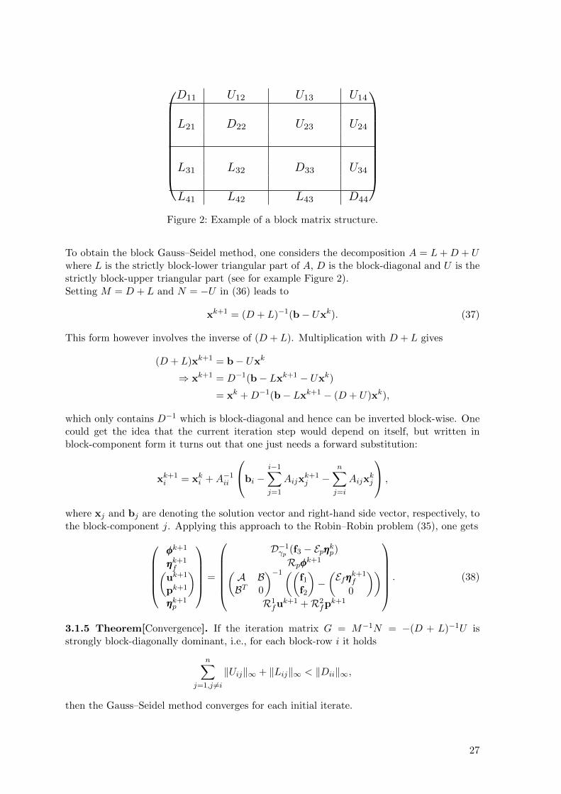
Figure 2: Example of a block matrix structure.

To obtain the block Gauss–Seidel method, one considers the decomposition A = L+D + Uwhere L is the strictly block-lower triangular part of A, D is the block-diagonal and U is thestrictly block-upper triangular part (see for example Figure 2).Setting M = D + L and N = −U in (36) leads to

xk+1 = (D + L)−1(b− Uxk). (37)

This form however involves the inverse of (D + L). Multiplication with D + L gives

(D + L)xk+1 = b− Uxk

⇒ xk+1 = D−1(b− Lxk+1 − Uxk)

= xk +D−1(b− Lxk+1 − (D + U)xk),

which only contains D−1 which is block-diagonal and hence can be inverted block-wise. Onecould get the idea that the current iteration step would depend on itself, but written inblock-component form it turns out that one just needs a forward substitution:

xk+1i = xki +A−1

ii

bi −

i−1∑

j=1

Aijxk+1j −

n∑

j=i

Aijxkj

,

where xj and bj are denoting the solution vector and right-hand side vector, respectively, tothe block-component j. Applying this approach to the Robin–Robin problem (35), one gets

φφφk+1

ηηηk+1f(

uk+1

pk+1

)

ηηηk+1p

=

D−1γp (f3 − Epηηηkp)Rpφφφk+1

(A BBT 0

)−1((f1

f2

)−(Efηηηk+1

f

0

))

R1fu

k+1 +R2fp

k+1

. (38)

3.1.5 Theorem[Convergence]. If the iteration matrix G = M−1N = −(D + L)−1U isstrongly block-diagonally dominant, i.e., for each block-row i it holds

n∑

j=1,j 6=i‖Uij‖∞ + ‖Lij‖∞ < ‖Dii‖∞,

then the Gauss–Seidel method converges for each initial iterate.

27

Proof. The iteration matrix fulfills the following relation:

G = M−1N = −(D + L)−1U ⇔ (D + L)G = −U ⇔ DG+ LG = −U⇔ DG = −LG− U⇔ G = −D−1(LG+ U).

Now let z ∈ Rd, z 6= 0, then i-th block-component of the relation is given by

(Gz)i = −D−1ii

i−1∑

j=1

Lij(Gz)j +

n∑

j=i+1

Uijzj

.

Having a closer look at the first block-component yields

‖(Gz)1‖∞ ≤ ‖D−111 ‖∞

n∑

j=2

‖U1j‖∞‖zj‖∞ ≤ ‖z‖∞1

‖D11‖∞

n∑

j=2

‖U1j‖∞ < ‖z‖∞

as the considered matrix is strongly block-diagonally dominant. Now we can prove theinequality for the other rows by induction: Suppose it holds for all j < i, then we canestimate

‖(Gz)i‖∞ ≤1

‖Dii‖∞

i−1∑

j=1

‖Lij‖∞‖(Gz)j‖∞ +n∑

j=i+1

‖Uij‖∞‖zj‖∞

≤ 1

‖Dii‖∞

i−1∑

j=1

‖Lij‖∞‖z‖∞ +n∑

j=i+1

‖Uij‖∞‖z‖∞

, induction hypothesis,

< ‖z‖∞ , strong diagonal dominance,

and it follows with‖(Gz)i‖∞ < ‖z‖∞ ⇒ ‖Gz‖∞ < ‖z‖∞,

that

ρ(G) ≤ ‖G‖∞ = maxz∈Rd,z 6=0

‖Gz‖∞‖z‖∞

< 1.

The first inequality holds, because for any eigenvalue - eigenvector pair (λ, z) of G it is

|λ|‖z‖∞ = ‖λz‖∞ = ‖Gz‖∞ ≤ ‖G‖∞‖z‖∞⇒ ρ(G) ≤ ‖G‖∞.

3.1.6 Remark[Convergence of the Stokes–Darcy system for K, ν → 0]. In order to be able toapply Theorem 3.1.5 to the Stokes–Darcy problem with Neumann–Neumann system matrix(31), the strong block-diagonal dominance has to hold. In the system matrix of the Darcysystem, each entry depends linearly on K. This means that if K → 0, the condition isviolated as the blocks which couple the systems do not depend on K at all.For the Stokes block, there is still the bilinear form b(·, ·) which does not depend on ν, henceν → 0 does not necessarily mean that the theorem does not hold.However, using the Robin–Robin system matrix (35) of the Stokes–Darcy problem results inan additional term in the Darcy part of the system, which does not scale with K. Hence,convergence might be recovered.

28

3.1.7 Remark[Block Jacobi method]. Another classic approach for iteratively solving asystem of equations is the block Jacobi method. Set M = D and N = −(L + U) and theiteration matrix is G = M−1N = −D−1(L+ U). Then the fixed point equation is

xk+1 = D−1(b− (L+ U)xk) = xk +D−1(b−Axk).

In contrast to the block Gauss–Seidel method, this iteration does not need a forward substi-tution and hence can be parallelized. Applying this approach to the Robin–Robin problem(35) one gets

φφφk+1

ηηηk+1f(

uk+1

pk+1

)

ηηηk+1p

=

φφφk

ηηηkf(uk

pk

)

ηηηkp

+

D−1γp (f3 −Dγpφφφk − Epηηηkp)

Rpφφφk − ηηηkf(Aγf BBT 0

)−1((f1 − Efηηηkf

f2

)−(Aγf BBT 0

)(uk

pk

))

R1fu

k +R2fp

k − ηηηp

.

3.2 Navier–Stokes–Darcy problem

The interface conditions as well as the general setting of domain and boundary is identicalto the Stokes–Darcy case. The Navier–Stokes–Darcy problem therefore reads as follows:Find (uf , pf , ϕp) : Ωf × Ωf × Ωp → Rd×R×R such that

−∇ ·T(uf , pf ) + (uf · ∇) · uf = ff in Ωf ,∇ · uf = 0 in Ωf ,

−∇ ·K∇ϕp = fp in Ωp,

uf = uf,ess on Γf,e,T(uf , pf ) · nf = Tf,nat on Γf,n,

ϕp = ϕp,ess on Γp,e,(−K∇ϕp) · nf = up,nat on Γp,n,

uf · nf = −(K∇ϕp) · nf on Γ,−nf ·T(uf , pf ) · nf = gϕp on Γ,

uf · τττ i + α0τττ i ·T(uf , pf ) · nf = 0 on Γ, i = 1, . . . , d− 1.

(39)

The only new part is the nonlinear convection-term (uf · ∇) · uf , otherwise the problem issimilar to (24). Therefore the weak formulation only differs a bit, too, as it now includes thein (16) defined trilinear form:

(i) Neumann–Neumann (see (30)): Find (uf , pf , ϕp) ∈ Vf ×Qf ×Qp such that

af (uf ,v) + bf (v, pf ) + c(uf ,uf ,v) + 〈gϕp,v · nf 〉Γ = 〈f1f ,v〉,

bf (uf , q) = 〈f2f , q〉,

ap(ϕp, ψ)− 〈uf · nf , ψ〉Γ = 〈fp, ψ〉,(40)

for all (v, q, ψ) ∈ Vf ×Qf ×Qp.

(ii) Robin–Robin (see (33)): Find (uf , pf , ϕp) ∈ Vf ×Qf ×Qp such that

af (uf ,v) + bf (v, pf ) + c(uf ,uf ,v) + 〈gϕp,v · nf 〉Γ+〈γfuf · nf ,v · nf 〉Γ + 〈γf (K∇ϕp) · nf ,v · nf 〉Γ = 〈f1

f ,v〉,bf (uf , q) = 〈f2

f , q〉,ap(ϕp, ψ) + 〈 1

γpϕp, ψ〉Γ + 〈 1

γpnf ·T(uf , pf ) · nf , ψ〉Γ − 〈uf · nf , ψ〉Γ = 〈fp, ψ〉,

(41)

29

for all (v, q, ψ) ∈ Vf ×Qf ×Qp.

The finite element discretization does not change much as well, just that A (or Arob, Aγfrespectively) now depend on uf due to the nonlinearity, i.e., the (i, j)-th component of thematrix now has the additional term

c(uf ,wj ,wi).

This issue can be resolved by the fixed point iterations seen in Section 2.3.2. Applying thefixed point iterations means that one has to solve either the whole system at once iteratively,or that one approximates the nonlinearity within a block-iterative method, like the Gauss–Seidel method presented in the following section.

3.2.1 Iterative approach

We will only discuss the case of the interface-coupled Robin–Robin method, as the Neumann–Neumann method can be obtained with γf = 0 and γp →∞.Let η0

f , η0p and γf , γp be given, as well as an initial guess φφφ0

p , e.g., the zero vector. Then thesequential or Gauss–Seidel type iteration looks like follows: Set k = 0, then following (38):

(i) Solve the Darcy problem with Robin boundary data ηkp :

Dγpφφφk+1 = f3 − Epηηηkp

and obtain φφφk+1.

(ii) Calculate ηηηk+1f = Rpφφφk+1

p .

(iii) Solve the Navier–Stokes problem with given interface-boundary ηηηk+1f :

(Aγf (uk+1) Brob

−BTrob 0

)(uk+1f

pk+1f

)=

(f1 − Efηηηk+1

f

f2

)

and obtain (uk+1f , pk+1

f ).

(iv) Calculate ηηηk+1p = R1

fuk+1f +R2

fpk+1f .

(v) If not converged, go back to step (i) and increase k by one.

The crucial step for the Navier–Stokes–Darcy problem is step (iii). There, one actually hasto solve equations with the nonlinear term

(Aγf (ukf ))ij = af (wj ,wi) + 〈γfwf · nf ,wi · nf 〉+ c(ukf ,wj ,wi).

This issue can be resolved in two ways:

• One can simply use the fixed-point iteration which was introduced in Section 2.3.2.Therefore one rewrites step (iii):

(iii).1 Solve the Navier–Stokes problem for uk,mf with given interface-boundary ηηηk+1f by

using the fixed point iterations, with the starting guess uk+1,0f = ukf until

(Aγf (uk+1,m) Brob

−BTrob 0

)(uk+1,m+1f

pk+1f

)=

(f1 − Efηηηk+1

f

f2

)

converges at iteration m0. Now set uk+1f := uk+1,m0

f and proceed with step (iv).

30

• One could also linearize only with the previous step ukf . This corresponds to do justone fixed point iteration.

(iii).2 Solve the linear problem

(Aγf (uk) Brob

−BTrob 0

)(uk+1f

pk+1f

)=

(f1 − Efηηηk+1

f

f2

)

for given wk.

In the first case one just iterates until a stopping criterion is reached. In the second casethere is only one iteration per step. One could argue, that the full iterations in the first caseare not needed, as the boundary conditions on the interface are not correct at least at thebeginning (i.e., for small k).

3.2.1 Remark[Parallelized algorithm]. As it was mentioned in Remark 3.1.7, it is alsopossible to use a parallelized block Jacobi method instead of the sequential block Gauss–Seidel method. The algorithm then is: Set k = 0, then

(i) Parallel:

Solve the Darcy problem with use of ηηηkp and obtain ϕϕϕk+1.

Solve the Navier–Stokes problem with use of ηηηkf and obtain (uk+1f ,pk+1

f ).

(ii) Parallel:

Update ηηηkf to ηηηk+1

f .

Update ηηηkp to ηηηk+1p .

(iii) If not converged, increase k by one and continue with step (i).

Note that this algorithm actually is not a pure Jacobi method, as the second step relies onthe solutions of the first step. It is rather a nested Jacobi and Gauss–Seidel method, seeSection 3.1 of [5].

4 Numerical studies

This chapter is about the comparison between the numerical solution of the Navier–Stokes–Darcy problem and a given analytical solution, especially in Example 1, as well as the com-parison between Example 2 (riverbed example) and results from the literature, see [7, 6].Also it is going to be analyzed, how the choice of the algorithm for the nonlinear part (i.e.,full iterations or just one iteration) impacts the costs to solve the whole system. For eachsolving process of a subsystem, a direct solver was used.

For the finite element discretization the spaces P2 and P1 were used for Navier–Stokes velocityand pressure respectively and P2 for the Darcy pressure as in [5]. The choice of finite ele-ments for Navier–Stokes velocity and pressure is also known as the Taylor–Hood element andpreserves the discrete variant of the inf-sup condition, see Chapter VI of [3]. This conditionis needed to assure uniqueness for the discrete problem, see Chapter 2 of [1].

4.1 Example 1

This example deals with a Navier–Stokes–Darcy problem of which the analytical solution isknown. Let Ωf = (0, 1)× (1, 2) and Ωp = (0, 1)2 with interface Γ = ∂Ωf ∩ ∂Ωp = (0, 1)×1.

31

f

p

(0,0)

(1,1)

(1,2)top

f,e

f

p

Figure 3: Example 1: Sketch of the domain (left) and triangulation of the domain on level 1(right).

The solution is given by

uf (x, y) =

(y2 − 2y + 1x2 − x

),

pf (x, y) = 2ν(x+ y − 1) +g

3K,

ϕp(x, y) =1

K

(x(1− x)(y − 1) +

y3

3− y2 + y

).

The set of equations to solve is

−∇ ·T(uf , pf ) + (uf · ∇) · uf =

((2y − 2)(x2 − x)

(2x− 1)(y2 − 2y + 1)

)in Ωf ,

∇ · uf = 0 in Ωf ,−∇ ·K∇ϕp = 0 in Ωp,

uf =

(y2 − 2y + 1

0

)on Γlr

f,e = 0, 1 × (1, 2),

uf =

(1

x2 − x

)on Γtop

f,e = (0, 1)× 2,

ϕp = 1K (y

3

3 − y2 + y) on Γlr

p,e = 0, 1 × (0, 1),

ϕp = 1K (x(x− 1)) on Γlow

p,e = (0, 1)× 0,

32

Type Algorithm Iterations Level 1 Level 2 Level 3 Level 4

Neumann–Neumann

Jacobiinterface 13 13 13 12nonlinear 31 29 29 25

total 44 42 42 37

Gauss–Seidelinterface 8 8 8 7nonlinear 20 19 19 17

total 28 27 27 24

Robin–Robin

Jacobiinterface 42 42 42 40nonlinear 65 65 63 61

total 107 107 105 101

Gauss–Seidelinterface 22 22 21 21nonlinear 38 39 37 37

total 60 61 58 58

Table 1: Example 1: Number of iterations of the Robin–Robin algorithm in comparison tothe Neumann–Neumann algorithm, using either the Jacobi method or the Gauss–Seidel method. The number of fixed-point iterations (here denoted as ”nonlinear”iterations) for solving the Navier–Stokes system had no limit.

plus the interface conditions (26), (27), the Beavers–Joseph–Saffman condition (28) on Γ =(0, 1) × 1 with nf = (0,−1)T and τττ id−1

i=1 = (1, 0)T . This example coincides mostlywith Example 2 (Section 4.2) of [5] with the difference that the Stokes equations have beenconsidered there. Therefore the right-hand side of the nonlinear Navier–Stokes equation hasto change in order to obtain the same solution.The grid consists, similar to Example 2 of [5], of triangles like shown in Figure 3.The following tests were run for γp = 1, γf =

γp3 , K = I and ν = 1 on four unstructured grids

with 470 (level 1), 1914 (level 2), 8216 (level 3) and 33234 (level 4) cells with a total of 1690(level 1), 6553 (level 2), 27402 (level 3) and 109613 (level 4) degrees of freedom.For the interface iterations the following condition has been used as stopping criterion:

‖uk+1f − ukf‖`2‖ukf‖`2

+‖pk+1f − pkf‖`2‖pkf‖`2

+‖ϕk+1

p − ϕkp‖`2‖ϕkp‖`2

< 10−10. (42)

The fixed-point iterations to solve the Navier–Stokes system stopped when the `2-norm ofthe residual vector was smaller than 10−10.First goal is to compare the Neumann–Neumann method (see Section 3.1.3) to the Robin–Robin method (see Section 3.1.5), as well as the performance of the Gauss–Seidel method(see Section 3.1.7) in comparison to the Jacobi method (see Remark 3.1.7).In order to compare these things, one needs some kind of measure for the costs. The numberof nonlinear iterations for solving the Navier–Stokes system were chosen for this matter. Thenumber of solving the Darcy system is negligible as it does not change per interface iterationand hence a factorization needs to be computed only once.In Table 1 one can see that the Neumann–Neumann method behaves better than the Robin–Robin method in terms of performed iterations. In this case, the Gauss–Seidel methodis more or less twice as fast as the Jacobi method. And even though the Jacobi methodcan be parallelized, which is not possible with the Gauss–Seidel method due to the forward

33

substitution performed in each step, the parallelization can only be applied to the two coupledsystems, hence there would be onyly little performance gain compared to the Gauss–Seidelmethod.

The Table 1 also shows the number of fixed-point iterations needed to solve the Navier–Stokessystem in total, but if one has a look at for example Figure 4, there are much more fixed-pointiterations for the nonlinear term in the beginning than in the end. For the other cases, thesame behavior can be observed. This leads to the question whether restricting the number ofiterations for the nonlinear term might lead to less iterations in total. The table also shows,that the number of iterations is independent of the mesh in all cases.

220 2 4 6 8 10 12 14 16 18 20

6

0

1

2

3

4

5

Interface iteration at

Fixe

d-po

int i

tera

tions

per

form

ed

Figure 4: Example 1: The number of fixed-point iterations needed over all interface iterations.The Robin–Robin method with Gauss–Seidel algorithm on level 4 was used.

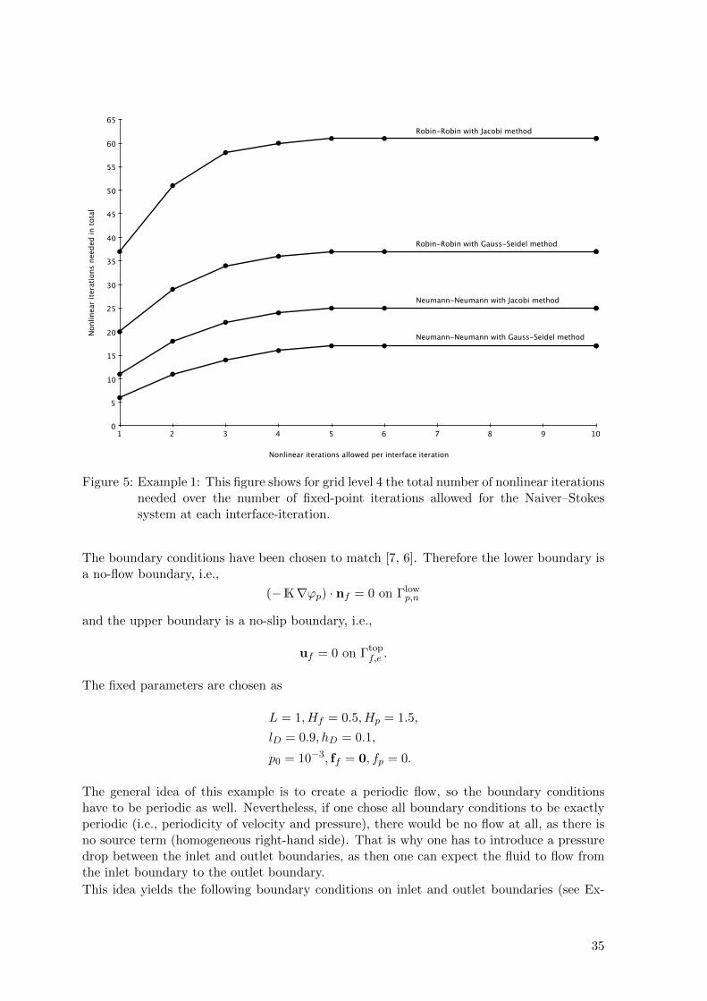
Having a look at Figure 5 shows at the example of grid level 4, that it seems to be mostconvenient to make just one fixed-point iteration in each step. This approach was presentedin Section 3.2.1.

4.2 Example 2 (riverbed example)

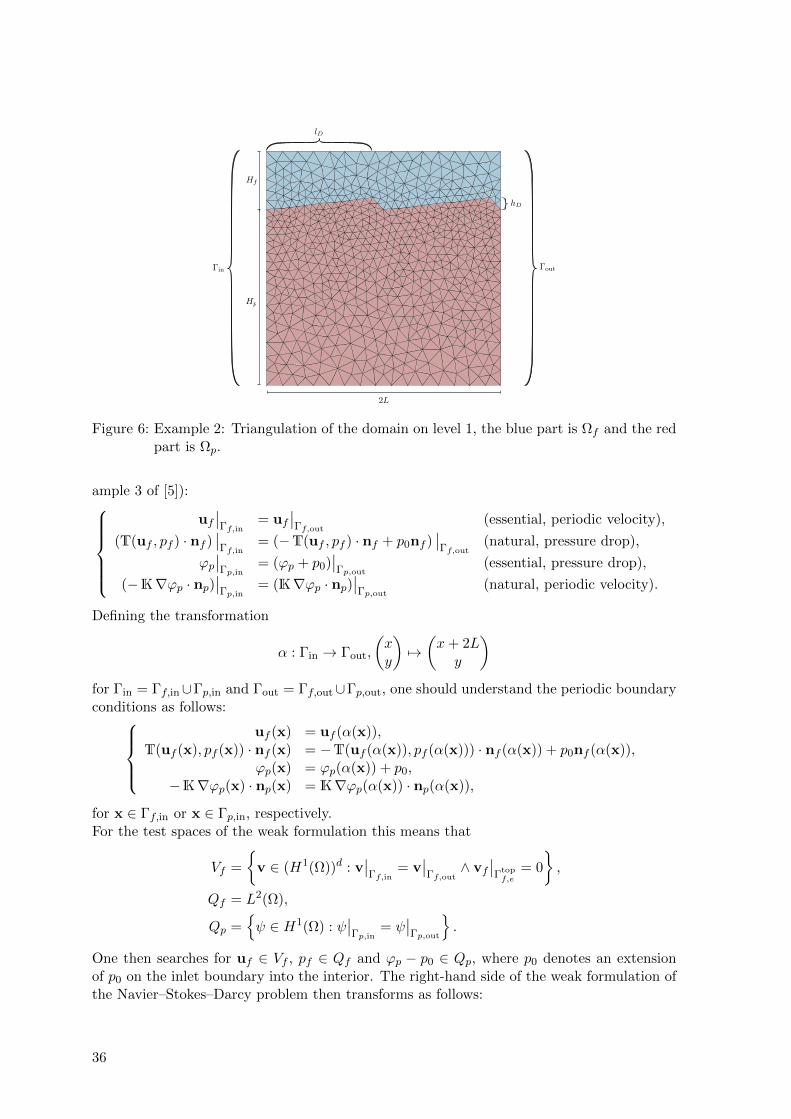
This example deals with the flow of a river over a porous riverbed with a periodic dune-shaped(modeled as triangles) interface. It was used for example in [7, 6] to study the hydrodynamicinteractions between the water flow and the underlying groundwater flow. Therefore considerthe domain

Ω = (0, 2L)× (0, Hf +Hp)

where Hf and Hp denote the initial heights of the water flow domain and the groundwaterflow domain respectively. The interface representing the dune consists of two triangles whosehighest points are at

x1 = lD, x2 = L+ lD, for 0 < lD < L

with the height (relative to the height of the interface-entrance point) hD, see Figure 6.

34

101 2 3 4 5 6 7 8 9

65

0

5

10

15

20

25

30

35

40

45

50

55

60

Nonlinear iterations allowed per interface iteration

Non

linea

r ite

ratio

ns n

eede

d in

tota

l

Robin-Robin with Jacobi method

Robin-Robin with Gauss-Seidel method

Neumann-Neumann with Gauss-Seidel method

Neumann-Neumann with Jacobi method

Figure 5: Example 1: This figure shows for grid level 4 the total number of nonlinear iterationsneeded over the number of fixed-point iterations allowed for the Naiver–Stokessystem at each interface-iteration.

The boundary conditions have been chosen to match [7, 6]. Therefore the lower boundary isa no-flow boundary, i.e.,

(−K∇ϕp) · nf = 0 on Γlowp,n

and the upper boundary is a no-slip boundary, i.e.,

uf = 0 on Γtopf,e .

The fixed parameters are chosen as

L = 1, Hf = 0.5, Hp = 1.5,

lD = 0.9, hD = 0.1,

p0 = 10−3, ff = 0, fp = 0.

The general idea of this example is to create a periodic flow, so the boundary conditionshave to be periodic as well. Nevertheless, if one chose all boundary conditions to be exactlyperiodic (i.e., periodicity of velocity and pressure), there would be no flow at all, as there isno source term (homogeneous right-hand side). That is why one has to introduce a pressuredrop between the inlet and outlet boundaries, as then one can expect the fluid to flow fromthe inlet boundary to the outlet boundary.

This idea yields the following boundary conditions on inlet and outlet boundaries (see Ex-

35

lD

hD

Hf

Hp

2L

in out

Figure 6: Example 2: Triangulation of the domain on level 1, the blue part is Ωf and the redpart is Ωp.

ample 3 of [5]):

uf∣∣Γf,in

= uf∣∣Γf,out

(essential, periodic velocity),

(T(uf , pf ) · nf )∣∣Γf,in

= (−T(uf , pf ) · nf + p0nf )∣∣Γf,out

(natural, pressure drop),

ϕp∣∣Γp,in

= (ϕp + p0)∣∣Γp,out

(essential, pressure drop),

(−K∇ϕp · np)∣∣Γp,in

= (K∇ϕp · np)∣∣Γp,out

(natural, periodic velocity).

Defining the transformation

α : Γin → Γout,

(xy

)7→(x+ 2Ly

)

for Γin = Γf,in∪Γp,in and Γout = Γf,out∪Γp,out, one should understand the periodic boundaryconditions as follows:

uf (x) = uf (α(x)),T(uf (x), pf (x)) · nf (x) = −T(uf (α(x)), pf (α(x))) · nf (α(x)) + p0nf (α(x)),

ϕp(x) = ϕp(α(x)) + p0,−K∇ϕp(x) · np(x) = K∇ϕp(α(x)) · np(α(x)),

for x ∈ Γf,in or x ∈ Γp,in, respectively.For the test spaces of the weak formulation this means that

Vf =

v ∈ (H1(Ω))d : v

∣∣Γf,in

= v∣∣Γf,out

∧ vf∣∣Γtopf,e

= 0

,

Qf = L2(Ω),

Qp =ψ ∈ H1(Ω) : ψ

∣∣Γp,in

= ψ∣∣Γp,out

.

One then searches for uf ∈ Vf , pf ∈ Qf and ϕp − p0 ∈ Qp, where p0 denotes an extensionof p0 on the inlet boundary into the interior. The right-hand side of the weak formulation ofthe Navier–Stokes–Darcy problem then transforms as follows:

36

(i) For each test function v ∈ Vf , it is

〈f1f ,v〉 = (f ,v)Ωf + 〈p0nf (α(x)),v(x)〉Γf,in ,

because

〈T(uf (x), pf (x)) · nf (x),v(x)〉Γf,n= 〈T(uf (x), pf (x)) · nf (x),v(x)〉Γf,in + 〈T(uf (α(x)), pf (α(x))) · nf (α(x)),v(α(x))〉Γf,in= 〈p0nf (α(x)),v(x)〉Γf,in ,

using v∣∣Γf,in

= v∣∣Γf,out

in the second step.

(ii) The second right-hand side 〈f2f , q〉 does not change.

(iii) For each test function ψ ∈ Qp, it is

〈K∇ϕp(x) · np(x), ψ(x)〉Γp,n= 〈K∇ϕp(x) · np(x), ψ(x)〉Γp,in + 〈K∇ϕp(α(x)) · np(α(x)), ψ(α(x))〉Γp,in= 0.

4.2.1 Remark. In the assembling process of the finite element system matrix the periodicboundary data are treated as follows:

• For each node on the inlet boundary, there is a corresponding node on the outletboundary. The condition

v∣∣Γf,in

= v∣∣Γf,out

or ψ∣∣Γp,in

= ψ∣∣Γp,out

tells, that these two nodes belong to the same basis function (which now takes value 1on both of the nodes). In order to assemble the matrix entries corresponding to thesespecial nodes correctly, first assemble them separately and treat the periodic bound-ary Γin and Γout as Neumann boundaries without the identifying condition v

∣∣Γf,in

=

v∣∣Γf,out

or ψ∣∣Γp,in

= ψ∣∣Γp,out

.

• With the help of basis functions of the Navier–Stokes velocity which take value 1 onthe inlet or on the outlet boundary, respectively, one has to construct basis functionsof Vf .

Therefore consider the (i, j)-th and the (k, j)-th entry of the Stokes matrix A, i.e.,

Aij = af (wj ,wi), Akj = af (wj ,wk),

with test functions wi and wk, such that the i-th column corresponds to a node xi ∈ Γin

and the k-th column corresponds to a node xk ∈ Γout with α(xi) = xk.

Replacing the i-th row by the sum of the k-th row and the old i-th row yields due tolinearity of the second argument

Aij = af (wj ,wi + wk).

This corresponds to take test functions wi + wk ∈ Vf .

The k-th entry of the right-hand side needs to be added to the i-th entry of the right-hand side as well.

37

ν K γp γftotal iterations on grid nonlinear iterations on grid

level 1 level 2 level 3 level 1 level 2 level 3

10−4 10−31 3 37 39 39 18 19 1910 30 35 39 37 17 19 18100 300 53 77 97 26 38 48

10−4 10−51 3 37 39 39 18 19 1910 30 35 41 39 17 20 19100 300 35 41 39 17 20 19

10−4 10−71 3 37 39 39 18 19 1910 30 35 41 39 17 20 19100 300 35 41 39 17 20 19

12 · 10−4 10−7

1 3 71 73 69 35 36 3410 30 71 73 73 35 36 36100 300 71 75 73 35 37 36

Table 2: Example 2: Total number of interface iterations and nonlinear iterations of theRobin–Robin algorithm with the Gauss–Seidel method for different choices of ν, K,γp, and γf . The number of nonlinear iterations is limited to 1 per interface iteration.

• Now the k-th row is set to zero with homogeneous right-hand side except for the (k, k)-th entry, which is set to 1, and the (k, j)-th entry, which is set to −1. With this, onegets the equality of velocity.

• The Darcy part of the matrix can be handled in the same way, just that one has inthe last step an inhomogeneous right-hand side, as the pressure drop in this case is anessential boundary condition.

In this example only the Robin–Robin method will be considered as the Neumann–Neumannmight not converge for small K, see Remark 3.1.6. For the domain three different unstruc-tured triangulations were used as shown in the following table:

Level interface edgescells degrees of freedom

Navier–Stokes Darcy Navier–Stokes Darcy

1 32 277 1009 1392 20982 68 1285 4513 6093 91963 138 5234 18322 24181 36987

As stopping criterion the same as in Example 1 has been used, see (42).The Robin–Robin method has parameters γf and γp so one could examine, which choiceof these parameters on which grid level is most efficient. Following the results of [5], onecould relate γf with γp by setting γf = 3γp. For measuring the costs, both the number ofnonlinear iterations and the total number of iterations (i.e., nonlinear and interface iterations)are considered. Table 2 shows, that the number of iterations is mostly independent of themesh. The algorithm performed well for all choices of γf and γp. The number of iterationsincreased rapidly with a smaller choice of ν. For larger K, smaller γp and γf seem to be more

38

convenient. Note that ν = 12 · 10−4 was the smallest number possible before the nonlinear

iterations did not converge anymore. In order to solve this arising instability, one has toconsider the time dependent equations.As ν = 1

Re seems to have a great impact on the iterations, one could have a look at therestrictions of the nonlinear iterations per interface iterations. Figure 7 shows, that indeedthe number of iterations grows rapidly with larger Reynolds numbers. It also shows that,when measuring the costs in terms of total iterations needed, in comparison to Figure 5,a larger Reynolds number shifts the optimal number of allowed nonlinear iterations perinterface iteration to greater numbers than 1 (in this example for Re = 2 · 104, a restrictionof 3 nonlinear iterations is most efficient). If considering just the nonlinear iterations neededas measure of cost, this observation cannot be made.In the papers [7, 6] it was suggested to do no interface iterations and just solve the Navier–Stokes system fully and then solve the Darcy system once. Figure 8 shows, that there isno qualitative impact. Compared to the Stokes–Darcy problem, the plots of Figure 8 showas well that the Navier–Stokes solution has eddies where the Stokes solution has not. Indirect comparison with Figure 1 of [6], one can clearly see that in Ωp there are the mentionedexchange, flow, and underflow areas.

39

201 2 3 4 5 6 7 8 9 10 11 12 13 14 15 16 17 18 19

90

25

30

35

40

45

50

55

60

65

70

75

80

85

Nonlinear iterations allowed per interface iteration

Inte

rfac

e it

erat

ions

and n

onlin

ear

iter

atio

ns

nee

ded

in t

otal

Re=1e2

Re=5e2

Re=1e3

Re=5e3

Re=1e4

Re=2e4

201 2 3 4 5 6 7 8 9 10 11 12 13 14 15 16 17 18 19

80

0

10

20

30

40

50

60

70

Nonlinear iterations allowed per interface iteration

Non

linea

r it

erat

ions

nee

ded

in t

otal

Re=1e2

Re=5e2

Re=1e3

Re=5e3

Re=1e4

Re=2e4

Figure 7: Example 2: This figure shows for grid level 2 with K = 10−5, γp = 100 andγf = 300 the total number of iterations needed (upper part) and the total numberof nonlinear iterations (lower part) needed, respectively, over the number of fixed-point iterations allowed for the Naiver–Stokes system at each interface-iteration.

40

K = 103, full interface iterations

K = 107, full interface iterations

K = 103, no interface iterations

K = 107, no interface iterations

K = 107, Stokes–Darcy systemK = 103, Stokes–Darcy system

Figure 8: Example 2: Numerical solution of the Navier–Stokes–Darcy system (upper fourplots) and the Stokes–Darcy system (lower two plots) for ν = 10−4, K ∈10−3, 10−7 on grid level 3. The lines represent the velocity field uf and ∇ϕp,respectively, mean flow is from left to right. All plots are colored according to thepressure field, scaled such that the minimum value is zero.

41

5 Conclusion and outlook

This thesis discussed the Navier–Stokes–Darcy problem as an extension of the Stokes–Darcyproblem. In particular it compared the Gauss–Seidel method to the Jacobi method forperforming the subdomain iterations which arise from the Neumann–Neumann method or theRobin–Robin method. Also it has been investigated which restrictions of nonlinear iterationsper interface iterations result in the lowest overall costs needed for convergence.When using the Gauss–Seidel method in comparison to the Jacobi method, it turns out thatthe Gauss–Seidel method needs only half the number of the iterations. However it cannotbe parallelized. Parallelization of the Jacobi method would reduce the needed time by atmost 50%. Altogether this means that the Gauss–Seidel method is the better choice in thiscase, as it is as fast as the parallelized Jacobi method but behaves better in terms of needediterations and computational costs.Using the Gauss–Seidel method, the Neumann–Neumann coupling might not be the rightchoice for small numbers of hydraulic permeability K, because Theorem 3.1.5 requires strongblock-diagonal dominance in order to guarantee convergence of the method for each startingvector and the entries of the Darcy part of the system matrix linearly depend on K. TheRobin–Robin method however has another term in the entries of the Darcy part of the systemmatrix, which does not depend on K but linearly on γ−1

p . Hence an appropriate choice of γpmight recover strong block-diagonal dominance.As in the Navier–Stokes–Darcy problem also the nonlinearity of the Navier–Stokes systemhas to be resolved, one could ask whether a restriction of nonlinear iterations per interfaceiteration might give faster convergence. If one chooses to measure the costs by evaluatingthe number of nonlinear and interface iterations needed, the examples show that for smallReynolds numbers a restriction to one nonlinear iteration per interface iteration and for largeReynolds numbers a restriction to three nonlinear iterations per interface iteration givesoptimal convergence. However it still needs to be investigated how exactly these restrictionsof nonlinear iterations depend on the Reynolds numbers. If one chooses to measure the costsby just counting the number of nonlinear iterations, this observation cannot be made anda restriction to one nonlinear iteration per interface iteration gives optimal convergence inall cases. How to actually measure the costs depends on the problem. If a factorization ofthe Darcy system can be stored and reused, counting the nonlinear iterations only is moremeaningful. If this cannot be done, one might consider to measure the costs by countingboth, the nonlinear iterations and the interface iterations.Altogether, the Stokes–Darcy problem considered in [5] has successfully been extended tothe Navier–Stokes–Darcy problem. The numerical results of the riverbed example coincidequalitatively with results from [7, 6].Further investigations could consider, e.g., different iterative solvers for the nonlinear equationin order to get (faster) convergence, especially for large Reynolds numbers. Also the optimalchoice of γf and γp needs to be discussed. Since in the examples a direct solver is used for allsubproblems, one could ask if an iterative solver is more efficient, possibly with a restrictednumber of iterations. When solving the subproblems, preconditioning might be of interest aswell.

42

References

[1] I. Babuska. On the existence, uniqueness, and approximation of saddle-point problemsarising from lagrange multipliers. Rev. Fr. Autom. Inf. Rech. Oper, 8:129–151, 1974.

[2] S. P. Boyd and L. Vandenberghe. Convex optimization. Cambridge university press,2004.

[3] F. Brezzi and M. Fortin. Mixed and hybrid finite element methods. Springer-Verlag NewYork, Inc., 1991.

[4] T. Brocker. Analysis II. BI Wissenschaftsverlag, 1992.

[5] A. Caiazzo, V. John, and U. Wilbrandt. On iterative subdomain methods for thestokes–darcy problem. 2013.

[6] M. B. Cardenas and J. L. Wilson. Dunes, turbulent eddies, and interfacial exchangewith permeable sediments. Water Resources Research, 43(8), 2007.

[7] M. B. Cardenas and J. L. Wilson. Hydrodynamics of coupled flow above and belowa sediment–water interface with triangular bedforms. Advances in water resources,30(3):301–313, 2007.

[8] M. Discacciati and A. Quarteroni. Navier-stokes/darcy coupling: modeling, analysis,and numerical approximation. Revista Matematica Complutense, 22(2), 2009.

[9] V. Girault and P.-A. Raviart. Finite element approximation of the Navier-Stokes equa-tions. Springer-Verlag, Berlin, 1981.

[10] V. John. Numerical mathematics ii. 2013.

[11] C. Kanzow. Numerik linearer Gleichungssysteme: Direkte und iterative Verfahren.Springer-Lehrbuch. Springer London, Limited, 2005.

[12] N. G. Meyers and J. Serrin. H= w. In Proceedings of the National Academy of Science,volume 51, pages 1055–1056, 1964.

[13] P. Neff, D. Pauly, and K.-J. Witsch. Poincare meets korn via maxwell: Extending korn’sfirst inequality to incompatible tensor fields. arXiv preprint arXiv:1203.2744, 2012.

43

Ich versichere, dass ich die Arbeit selbststandig verfasst und keine anderen als die angegebenenQuellen und Hilfsmittel benutzt sowie Zitate kenntlich gemacht habe.

Berlin, den

44