Dr Fiona J. L. Reid Applications Consultant, EPCC

f.reid@epcc.ed.ac.uk +44 (0)131 651 3394

The NEMO Ocean Modelling Code: A Case Study

CUG 24th – 27th May 2010

CUG 24th - 27th May 2010 2

Acknowledgements

•  Cray Centre of Excellence team for their help throughout the project

•  Chris Armstrong, NAG for help with netCDF on the X2

CUG 24th - 27th May 2010 3

Talk outline

•  Overview of the NEMO dCSE Project

•  What is NEMO?

•  System introductions

•  XT results –  Baseline performance and optimisations –  netCDF 4.0 performance

–  Optimising NEMO I/O –  Nested model performance and troubleshooting

•  Achievements

CUG 24th - 27th May 2010 4

Overview of NEMO dCSE project

•  The NEMO Distributed Computational Science and Engineering

(dCSE) Project was a collaboration between EPCC and the

Ocean Modelling and Forecasting (OMF) group based at the

National Oceanography Centre, Southampton (NOCS).

•  The project was funded by a HECToR dCSE grant administered

by NAG Ltd on behalf EPSRC

•  The NEMO dCSE Project concentrated on the following areas:-

–  I/O performance on intermediate and large numbers of processors

–  Nested model performance

•  In addition, a separate project investigated porting NEMO to the

HECToR vector system, the X2

CUG 24th - 27th May 2010 5

What is NEMO?

•  NEMO (Nucleus for European Modelling of the Ocean) is a modelling framework for oceanographic research

•  Allows ocean related components, e.g. sea-ice, biochemistry, ocean dynamics, tracers, etc to work either together or separately

•  European code with the main developers based in France

•  Major partners include: CNRS, Mercator-Ocean, UKMO and NERC

•  Fortran 90, parallelised using MPI – versions 2.3 and 3.0

•  Code has previously run on both scalar and vector machines

•  This project uses the official releases (OPA9) with some NOCS specific enhancements

CUG 24th - 27th May 2010 6

•  HECToR (Phase 1): Cray XT4 –  MPP, 5664 nodes, 2 AMD Opteron 2.8 GHz cores per node –  6 GB of RAM per node (3 GB per core) –  Cray Seastar2 torus network

•  HECToR (Vector): Cray X2 –  Vector machine, 28 nodes, with 4 Cray X2 processors per

node –  32 GB of RAM per node (8 GB per Cray X2 processor) –  Cray YARC network

System introductions

XT results

CUG 24th - 27th May 2010 8

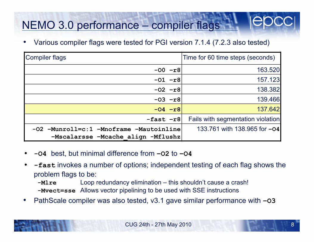
NEMO 3.0 performance – compiler flags •  Various compiler flags were tested for PGI version 7.1.4 (7.2.3 also tested)

•  -O4 best, but minimal difference from –O2 to –O4 •  -fast invokes a number of options; independent testing of each flag shows the

problem flags to be: -Mlre Loop redundancy elimination – this shouldn’t cause a crash! -Mvect=sse Allows vector pipelining to be used with SSE instructions

•  PathScale compiler was also tested, v3.1 gave similar performance with –O3

Compiler flags Time for 60 time steps (seconds)

-O0 –r8 163.520 -O1 –r8 157.123 -O2 –r8 138.382 -O3 –r8 139.466 -O4 –r8 137.642

-fast –r8 Fails with segmentation violation -O2 –Munroll=c:1 –Mnoframe –Mautoinline

–Mscalarsse –Mcache_align -Mflushz 133.761 with 138.965 for –O4

CUG 24th - 27th May 2010 9

NEMO performance – SN versus VN

•  HECToR can be run in single core (SN) or virtual node (VN) mode

•  SN mode uses one core per node, VN mode uses both cores •  If your application suffers from memory bandwidth problems SN mode

may help

•  Runtime reduces when running NEMO in SN mode

•  NEMO doesn’t benefit sufficiently to justify the increased AU usage

Number of processors

Time for 60 steps (seconds) SN mode VN mode

256 119.353 146.607

221 112.542 136.180

CUG 24th - 27th May 2010 10

NEMO grid

Grid used for ORCA025 model

jpni = number of cells in the horizontal direction

jpnj = number of cells in the vertical direction

Here, jpni = 18, jpnj = 12

Image provided courtesy of Dr Andrew Coward, NOCS

i direction

j dire

ctio

n

CUG 24th - 27th May 2010 11

NEMO performance – equal grid dims

CUG 24th - 27th May 2010 12

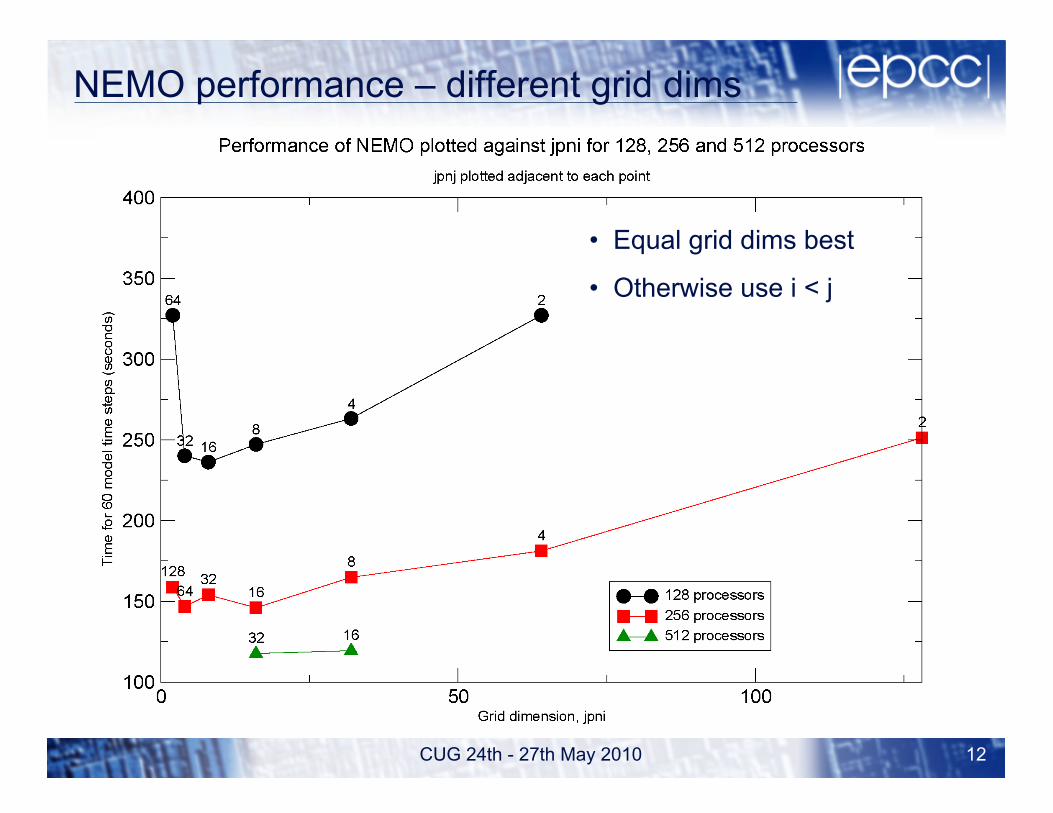
NEMO performance – different grid dims

•  Equal grid dims best

•  Otherwise use i < j

CUG 24th - 27th May 2010 13

NEMO performance – removal of land cells

•  Ocean models only model the ocean

•  Depending on the grid, some cells may contain just land –  Land only cells do not have any computation associated with them –  However, they do have I/O

–  A zero filled netCDF file is output for each land cell

•  The land only cells can be removed prior to running NEMO –  Work out how many land only cells there are via the bathymetry file

–  Set the value of jpnij equal to the number of cells containing ocean –  E.g. for a 16 x 16 grid there are 35 pure land cells so jpnij = 221

CUG 24th - 27th May 2010 14

NEMO performance – removal of land cells

•  Removal of land cells reduces the runtime and the amount of file I/O – No unnecessary output for land regions

•  In addition the number of AU’s required is greatly reduced – Up to 25% reduction for a 1600 processor run

jpni jpnj jpnij Reduction in AU’s used

Time for 60 steps (seconds)

8 16 128 236.182 8 16 117 8.59% 240.951

16 16 256 146.607 16 16 221 13.67% 136.180 16 32 512 117.642 16 32 420 17.97% 111.282 32 32 1024 110.795 32 32 794 22.46% 100.011

CUG 24th - 27th May 2010 15

NEMO performance – optimal proc count

•  NOCS researchers want to be able to run a single model year (i.e. 365 days) during a 12 hour run –  Aids the collation and post-processing of results

–  Current runs on 221 processors provide around 300 model days

•  Investigated the “optimal” processor count as follows –  Remove land cells –  Keep grid dimensions as close to square as possible

–  Compute the number of model days computed in 12 hours from: ndays = 43000/t60

–  Ideally want t60 to be ≤ 118 seconds

–  Investigated processor counts from 159 - 430

CUG 24th - 27th May 2010 16

NEMO performance – optimal proc count

Need to use ~320 processors to achieve the performance targets

CUG 24th - 27th May 2010 17

NEMO I/O

•  NEMO input & output files are a mixture of binary and ASCII data –  Several small input ASCII files which set key parameters for the run –  Several small output ASCII files; time step, solver data, run progress

–  Binary input files for atmospheric data, ice data, restart files etc –  Binary output file for model results, restart files etc

•  All binary data files are in netCDF format –  netCDF = network Common Data Format

–  Portable data format for storing/sharing scientific data

•  NEMO uses parallel I/O –  each processor writes out its own data files depending on which part

of the model grid it holds

–  Should be efficient but may suffer at larger processor counts…

CUG 24th - 27th May 2010 18

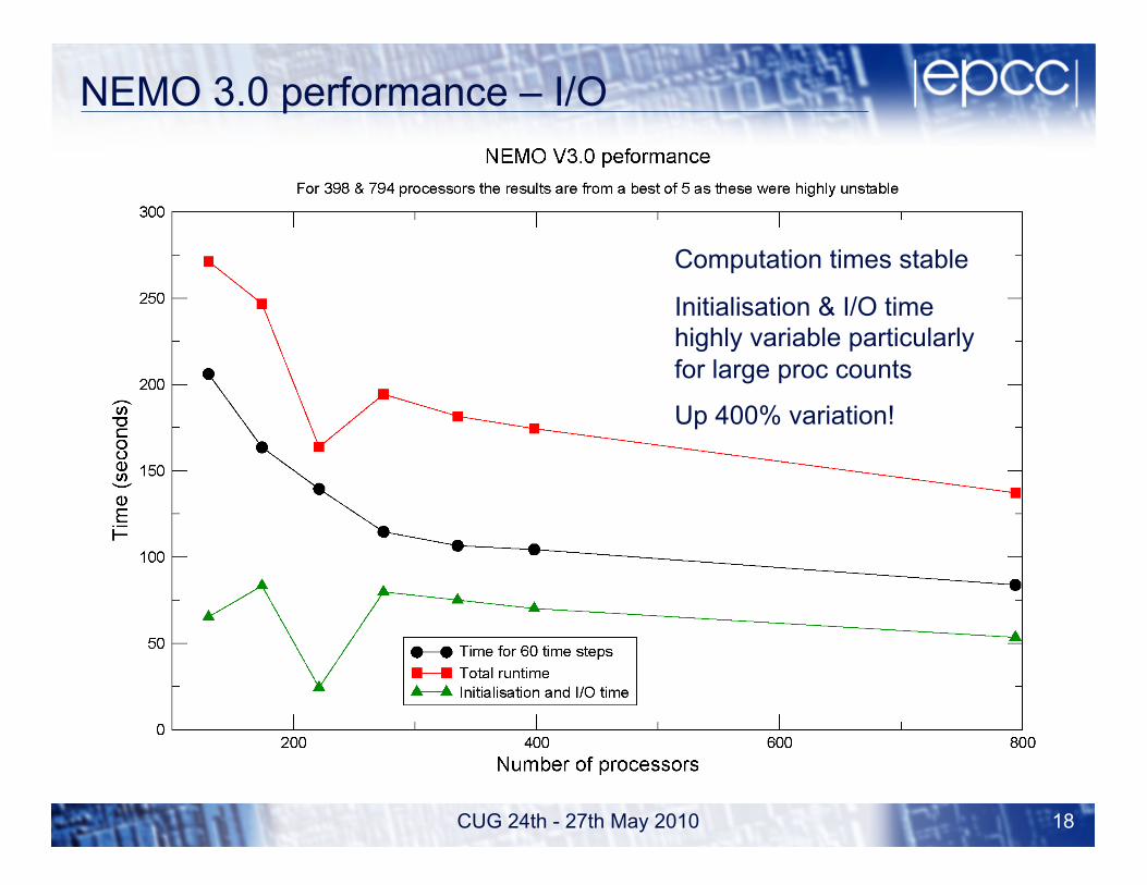
NEMO 3.0 performance – I/O

Insert graph for NEMO 3.0 here Computation times stable

Initialisation & I/O time highly variable particularly for large proc counts

Up 400% variation!

CUG 24th - 27th May 2010 19

netCDF 4.0

•  netCDF 4.0 was used to improve I/O performance of NEMO

•  Key features –  Lossless data compression and chunking

–  areas with the same numeric value require far less storage space

–  Backward compatibility with earlier versions

•  Requires:- –  HDF 5.0 1.8.1 or later

–  Zlib 1.2.3 –  Szip (optional)

•  All codes tested with supplied test suites – all tests pass –  Cross compiling caused a few hiccups

–  Now available centrally as Cray supported modules on HECToR

CUG 24th - 27th May 2010 20

netCDF 4.0 performance

•  Performance evaluated using the NOCSCOMBINE tool

•  NOCSCOMBINE is a serial tool written by the NOCS researchers which reads in multiple NEMO output files and combines them into a single file –  The entire file can be combined or

–  Single components e.g. temperature can be extracted

CUG 24th - 27th May 2010 21

netCDF 4.0 performance

•  NOCSCOMBINE compiled with various versions of netCDF

•  A single parameter (temperature) is extracted across 221 input files –  Minimal computation, gives a measure of netCDF & I/O performance

–  Time measured and the best (fastest) of 3 runs reported

–  netCDF 3.6.2 and 4.0 output compared using CDFTOOLS* to ensure results are correct

*CDFTOOLS – set of tools for extracting information from NEMO netCDF files

CUG 24th - 27th May 2010 22

netCDF performance

•  Compiler optimisation doesn’t help

•  System zlib 1.2.1 faster than version 1.2.3 – Use with care, netCDF 4.0 specifies zlib 1.2.3 or later

•  File size is 3.31 times smaller •  Performance of netCDF 4.0 is 4.05 times faster

– Not just the reduced file size, may be algorithmic changes, c.f. classic

•  Cray version ~ 18% slower than dCSE install (for this example)

netCDF version NOCSCOMBINE time (seconds)

File size (Mb)

3.6.2 classic 344.563 731 4.0 snapshot un-optimised 86.078 221

4.0 snapshot optimised 85.188 221 4.0 release 85.188 221

4.0 release* 78.188 221 4.0 Cray version 92.203 221

4.0 release classic 323.539 731

*system Zlib 1.2.1 used

CUG 24th - 27th May 2010 23

Converting NEMO to use netCDF 4.0

•  NEMO should benefit from netCDF 4.0 –  The amount of I/O and thus time spent in I/O should be significantly

reduced by using netCDF 4.0

•  NEMO was converted to use netCDF 4.0 as follows:- –  Convert code to use netCDF 4.0 in Classic Mode

–  Convert to full netCDF 4.0 without chunking/compression –  Implement chunking and compression

–  Test for correctness at each stage

–  Full details in the final project report

CUG 24th - 27th May 2010 24

NEMO performance with netCDF 4.0

Filename File size netCDF 3.X (MB)

File size netCDF 4.0 (MB)

Reduction factor

*grid_T*.nc 1500 586 2.56

*grid_U*.nc 677 335 2.02

*grid_V*.nc 677 338 2.00

*grid_W*.nc 3300 929 3.55

*icemod*.nc 208 145 1.43

*restart_0*.nc 9984 9984 1.00

*restart_ice*.nc 483 483 1.00

•  Up to 3.55 times reduction in file size

•  Actual performance gains will depend on output required by science

CUG 24th - 27th May 2010 25

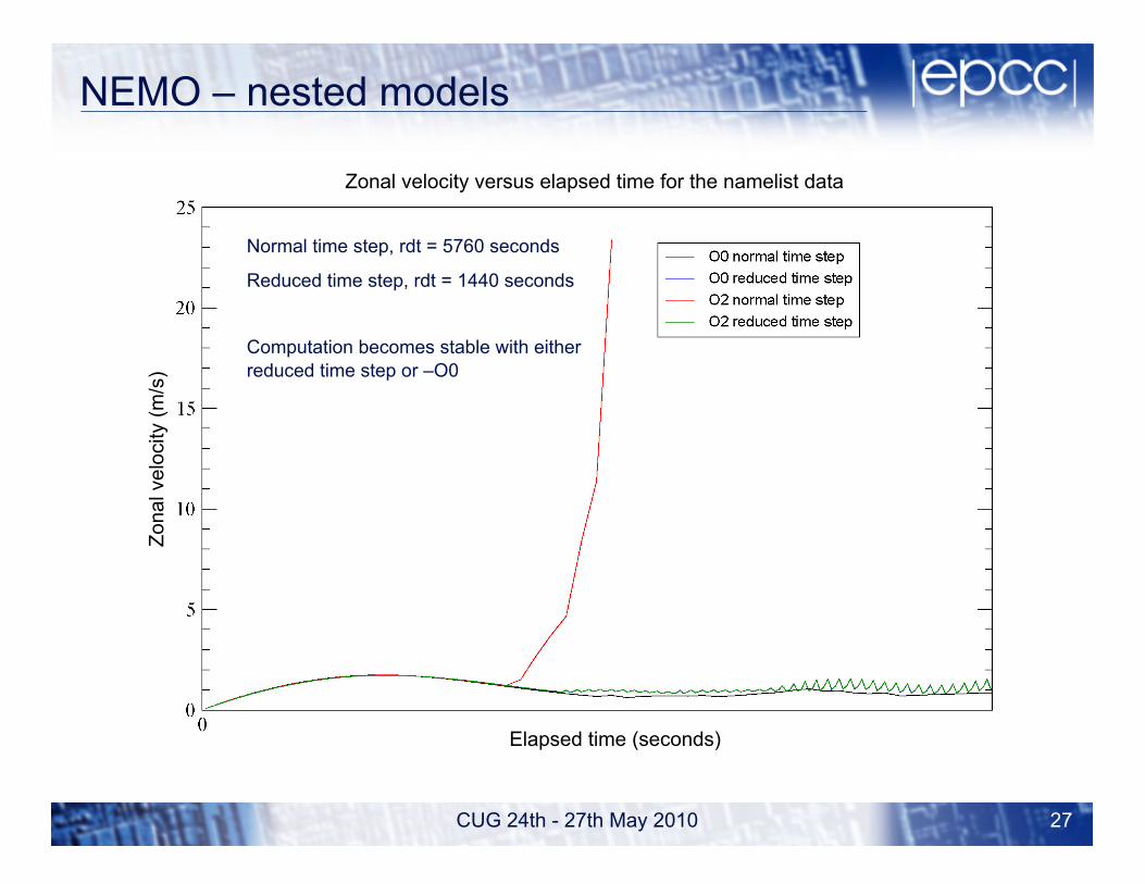
NEMO – nested models

•  Nested models – enable complex parts of the ocean to be studied at a higher resolution, e.g.

2º outer model

Two, 1º degree inner models

0.25º degree innermost model

Two models: BASIC, MERGED

BASIC: 2º model with a 1º nested model, no NOCS features

MERGED: 1º model with two 0.25º nested regions, NOCS code

Crashes with the velocity becoming unrealistically large

CUG 24th - 27th May 2010 26

NEMO – nested models •  BASIC model

–  Error occurs in outermost (i.e. un-nested) model –  Plot of velocity against time step highlights the problem

Zona

l vel

ocity

(m/s

)

Elapsed time (seconds)

Zonal velocity versus elapsed time for the namelist data

Normal time step, rdt = 5760 seconds

Reduced time step, rdt = 1440 seconds

Blue/green lines coincident

CUG 24th - 27th May 2010 27

NEMO – nested models Zo

nal v

eloc

ity (m

/s)

Elapsed time (seconds)

Zonal velocity versus elapsed time for the namelist data

Normal time step, rdt = 5760 seconds

Reduced time step, rdt = 1440 seconds

Computation becomes stable with either reduced time step or –O0

CUG 24th - 27th May 2010 28

NEMO – nested models

•  BASIC model –  Reducing level of optimisation or reducing the time step resolves the

problem for the BASIC model

•  MERGED model still an issue –  Velocity explodes for all levels of nesting –  Compiler flags and reduction of timestep do not help –  Thought to be an uninitialised value or memory problem –  Compiler & debugger bugs discovered limited further investigations

CUG 24th - 27th May 2010 29

NEMO - achievements

•  25% reduction in AU usage by removing land-only cells

•  Obtained optimal processor count for a 12 hour run on HECToR

•  Compiled netCDF 4.0, HDF5 1.8.1, zlib 1.2.3 and szip on HECToR

•  3 fold reduction in disk usage and 4 fold reduction in runtime with NOCSCOMBINE tool and netCDF4.0

•  Adapted NEMO to use netCDF 4.0 resulting in reduction in disk usage of up to 3.55 times

•  Resolved several issues with nested models crashing on HECToR

•  Found optimal processor count for BASIC nested model