the neoclassical revival in growth economics: has it … · the belief was that differences in...

This PDF is a selection from an out-of-print volume from the NationalBureau of Economic Research

Volume Title: NBER Macroeconomics Annual 1997, Volume 12

Volume Author/Editor: Ben S. Bernanke and Julio Rotemberg

Volume Publisher: MIT Press

Volume ISBN: 0-262-02435-7

Volume URL: http://www.nber.org/books/bern97-1

Publication Date: January 1997

Chapter Title: The Neoclassical Revival in Growth Economics: HasIt Gone Too Far?

Chapter Author: Peter Klenow, AndrÃ©s RodrÃ-guez-Clare

Chapter URL: http://www.nber.org/chapters/c11037

Chapter pages in book: (p. 73 - 114)

Peter J. Klenow and Andres Rodriguez-Clare GRADUATE SCHOOL OF BUSINESS, UNIVERSITY OF CHICAGO

The Neoclassical Revival

in Growth Economics: Has It Gone

Too Far?

1. Introduction Theories endogenizing a country's technology, such as Romer (1990) and Grossman and Helpman (1991), arose from the desire to explain the enormous disparity of levels and growth rates of per capita output across countries. The belief was that differences in physical and human capital intensity were not up to the quantitative task. This belief has been shaken by a series of recent empirical studies. Mankiw, Romer, and Weil (1992) estimate that the Solow model augmented to include human capital can explain 78% of the cross-country variance of output per capita in 1985. Alwyn Young (1994, 1995) finds that the East Asian growth miracles were fueled more by growth in labor and capital than by rising productivity. And Barro and Sala-i-Martin (1995) show that the augmented Solow model is consistent with the speed of convergence they estimate across countries as well as across regions within the United States, Japan, and a number of European countries.1

In our view these studies constitute a neoclassical revival.2 They suggest

We are grateful to Ben Bemanke, Mark Bils, V. V. Chari, Chad Jones, Greg Mankiw, Ed Prescott, David Romer, Julio Rotemberg, Jim Schmitz, Nancy Stokey, and Alwyn Young for helpful comments. 1. Mankiw, Romer, and Weil, and Barro and Sala-i-Martin do not explain the source of

country differences in investment rates. Chari, Kehoe, and McGrattan (1996) argue that distortions such as tax rates, bribes, risk of expropriation, and corruption contribute to an effective tax rate which, if it varies in the right (stochastic) way across countries, can explain the levels and growth rates of income observed in the Summers-Heston (1991) panel.

2. We are indebted to Alwyn Young for this phrase.

74 * KLENOW & RODRIGUEZ-CLARE

that the level and growth rate of productivity is roughly the same across countries, so that differences in output levels and growth rates are largely due to differences in physical and human capital. Romer (1993), in contrast, argues that "idea gaps" are much more important than "object gaps." In terms of a simplified production function Y = AX, where A is productivity and X encompasses physical and human capital, this debate is over the relative importance of A and X.

This debate matters because the positive and normative implications of the A view can differ dramatically from those of the X view. Technology- based models of A exhibit scale effects because of the nonrival nature of technology creation and adoption. And they suggest that openness, perhaps though its effect on technology diffusion, can have first-order effects on living standards and growth rates (without requiring big differences in rates of return to capital). These implications of openness could be positive in all countries, as in Rodriguez-Clare (1997), or positive in some and negative in others, as in Stokey (1991) and Young (1991). These implications are not shared by the basic neoclassical growth model, which has the same technology everywhere.

In this paper we offer new evidence relevant to this debate on the

importance of productivity vs. physical and human capital in explaining international differences in levels and growth rates of output. In Section 2 we reexamine Mankiw, Romer, and Weil's (hereafter MRW) methodol-

ogy for estimating human capital. We update their data and add data on

primary and tertiary schooling which have become available since their

study. Because primary school attainment varies much less across countries than secondary school attainment does, the resulting estimates of human capital vary much less across countries than the MRW estimates. We also incorporate evidence suggesting that the production of human

capital is more labor-intensive and less physical capital-intensive than is the production of other goods. This further narrows country differences in estimated human capital stocks.

In Section 3 we incorporate evidence that pins down the human capital intensity of production and the relative importance of primary vs.

secondary schooling. We exploit information contained in Mincer regressions, commonly run in the labor literature, on the amount of human

capital gained from each year of schooling. For a cross section of workers, Mincer (1974) ran a regression of worker log wages on worker years of schooling and experience. Such regressions have since been run for

many countries (see Bils and Klenow, 1996, for citations for 48 countries). We combine this evidence with data on schooling attainment and estimates of school quality to produce measures of human capital for 98 countries. Using these Mincer-based estimates of human capital, we find

The Neoclassical Revival in Growth Economics * 75

that productivity differences account for half or more of level differences in 1985 GDP per worker.3

In Section 4 we carry out the same analysis as in Section 3, but here the

objective is to produce 1960-1985 growth rates rather than 1985 levels. We find that differences in productivity growth explain the overwhelm-

ing majority of growth rate differences. These results seem at odds with

Young (1994, 1995), so in Section 5 we compare and contrast our findings for 98 countries with his careful findings for four East Asian countries.

Hall and Jones (1996) also follow Bils and Klenow (1996) in using Mincer regression evidence to construct human capital stocks. As we do, they find that productivity differences are important in explaining international income variation.4 Their main objective is different from ours, however, in that they are interested in finding correlates (such as lan-

guage and climate) with productivity differences. In contrast, we focus on examining how human capital should be measured and how international productivity differences depend on how human capital is measured. We want to know, for instance, whether our measure of human

capital is more appropriate than the one used by MRW, and we want to know how adding experience and correcting for schooling quality affects the results on productivity. Our paper also differs from Hall and Jones (1996) in that we study growth-rate differences as well as level differences, whereas they concentrate on level differences.5

3. OLS Mincer-equation estimates of the wage gain from each additional year of schooling might be too generous because of oft-cited ability bias (more able people acquire more education). In the NLSY over 1979-1993, we ran a Mincer regression of log (deflated wage) on schooling, experience, and experience squared and found a schooling coefficient of 9.3% (s.e. 0.1%). When we included the AFQT score as a proxy for ability, the estimated wage gain from each year of schooling fell to 6.8% (s.e. 0.2%). We stick with the standard estimates such as 9.3% for two reasons: first, since we will find that the role of human capital is smaller than MRW found, we prefer to err on the side of overstating variation in human capital across countries; second, the AFQT score could be a function of human capital investments in the home, and the overstated return may crudely capture how these investments tend to be higher when attainment is higher.

4. Hall and Jones reach quantitatively similar conclusions to ours because of two offsetting differences. First, as we will describe in Section 2 below, we take into account the natural effect of higher TFP on the capital-labor ratio (which increases to keep the return on capital at its steady-state equilibrium level) and therefore attribute the whole effect (i.e., higher TFP plus resulting higher capital-labor ratio) to higher productivity. Hall and Jones attribute only the direct effect to TFP, ignoring the indirect effect on the capital- labor ratio. Second, we estimate country differences in the quality of schooling that reinforce differences in the quantity of schooling attainment across countries. Hall and Jones look only at the quantity of schooling.

5. Bosworth, Collins, and Chen (1995) also estimate TFP growth rates with human capital stocks constructed using a methodology that is at some points close to ours. Instead of exploring the importance of differences in TFP growth rates in explaining international growth variation, these authors use such estimates of TFP growth to run cross-country TFP growth regressions.

76 * KLENOW & RODRiGUEZ-CLARE

2. Reexamining MRW In this section we first describe and comment on MRW's methodology for attributing differences in output to differences in productivity vs. differences in capital intensity. We then update MRW's estimates and make a series of modifications, such as incorporating primary school data and a more labor-intensive technology for producing human capital.

MRW specify the production technology

Y = C + IK + IH = KaHI(AL)'- a-, (1)

where Y is output, K and H are stocks of physical and human capital, A is a productivity index, and L is the number of workers. H = hL, where h is human capital per worker. Implicit is an infinite-lived representative agent whose time enters production through dual components, human

capital H and raw labor L.6 As shown in (1), MRW specify the same

technology for producing human and physical capital. Time subscripts are suppressed, as are the standard accumulation equations for K and H. MRW assume that both stocks depreciate geometrically at a rate of 3%

per year. If one adds competitive output and input markets and constant rela-

tive risk aversion utility, then it is well known that higher A will induce

proportionate increases in K and H. Given this fact, rather than the usual

accounting exercise that assigns output or its growth rate to contributions from K, H, L, and A, we think MRW rightly rearrange (1) to yield

Y / K a/(ia-) H\/(1-a-) L =A - = AX, (2) L Y.

where X is a composite of the two capital intensities. We concur with MRW's adoption of (2) for two reasons. First, Y/L is the object of interest rather than Y, since we want to understand why output per worker varies across countries, leaving aside how a country's number of workers L is determined.7 The A-vs.-X debate really has nothing to do with the determination of L. Second, (2) gives A "credit" for variations in K and H generated by differences in A. The contributions of K and H

6. Formally, the efficiency units contributed by a worker with human capital h are e = h(l -a)A(-a-)/(1-a), and the production function is Y = KEl-", where E = eL.

7. Parente, Rogerson, and Wright (1996) argue that hours worked in the market (as opposed to home production) by the average worker varies a lot across countries, making the number of workers a poor measure of market labor input. If, as these authors argue, market hours per worker are much higher in richer countries, it should contribute to higher A in richer countries.


variations that are not induced by A are captured by variations in capital intensity X. This decomposition was also adopted by King and Levine (1994), albeit for a setting with physical capital but not human capital.

We offer two caveats to the decomposition in (2), both related to A being endogenous, say resulting from technology adoption decisions.8 First, one would expect that many country policies affect both A and X. Weak enforcement of property rights in a country, for example, is likely to decrease both A and X. We think the decomposition in (2) is still useful, however, because there are some policies that could affect one factor much more than the other (e.g., education policies). Thus, finding that high levels of output per worker are explained mostly by high levels of H/Y would suggest that differences in education policies are an important element in explaining international differences in output per worker. Similarly, finding that differences in K/Y are important in accounting for the international variation in output per worker would point towards capital taxation or policies that affect the relative price of investment goods.

The second related caveat concerning the decomposition in (2) is that, just as K and H are affected by A, A itself may be affected by capital intensity X. If A is determined by technology adoption, for instance,

8. We do not list the embodiment of technology in physical capital as problematic for the decomposition in (2). Suppose that productivity entirely reflects the quality of physical capital, and that all countries invest in the highest quality capital goods available in the world in the period of investment. Then differences in country productivity levels could be due to differences in the vintage or age of a country's capital stock, i.e. unmeasured differences in the quality of a country's capital stock. In this situation, one might think (2) would attribute to productivity differences what in reality should be attributed to differences in physical capital intensity, say because countries with high investment rates and high capital intensity are using younger and therefore better equipment. If so, our results would understate the role of capital intensity in explaining international output differences. This concern turns out to be unfounded along a steady-state growth path. To see why, suppose the true, quality-adjusted capital stock evolves according to AKt = BtIt - 8Kt, where A is the first-difference operator and B is an exogenous capital-embodied technology index which grows at the constant rate g and (recall) is the same for all countries. Imagine also that the measured capital stock evolves according to AKMt = It - 8KMt so that it does not reflect improvements in quality coming from embodied technology. In this case one can show that if Y = K"L1l-, then along a steady-state growth path with constant IIY and KM/Y one has Y/Lt = (cBt)'(1-a)(KM/Y)a'/-a) with c a constant which depends on g, a, and 8, and with KM/Y = (IIY)/(g+n+8), where n is the exogenous growth rate of L. Thus, along a steady-state growth path, a country's TFP is independent of its investment rate in physical capital. That is, the investment rate does not affect the TFP residual, which in this case is equal to ln(Y/Lt) - a/(1 - a) In(K/Y), which in turn is equal to [1/(1 - a)] ln(cB,). The intuition for this result is that a higher investment rate reduces the average age of the capital only temporarily, along the transition path. When the new steady-state path is reached with higher capital intensity, the age distribution of the capital stock-which is synonymous with the quality distribution-is the same as the distribution with a lower capital intensity. Thus a country with a permanently higher IIY than another country will have no younger or better capital and therefore no higher TFP.

78 KLENOW & RODRIGUEZ-CLARE

then it is likely that higher schooling (i.e., higher H/Y) leads to a higher level of A. Once we obtain estimates of A and X, below we will actually use the decomposition of equation (2) to study this issue by looking at the correlation between A and the capital-intensity variables K/Y and H/ Y. A hypothetical example will illustrate the usefulness of this approach. Imagine that, using this decomposition, we find that almost all of the international variation in levels of Y/L is accounted for by international differences in A. But imagine that we also find a strong positive correlation between A and H/Y. This would be consistent with-but not neces-

sarily proof for-the view that human capital explains differences in Y/L, albeit indirectly through its effect on A (say through economywide tech-

nology adoption as in the model of Ciccone, 1994). On the other hand, finding no correlation between A and H/Y would suggest that differences in schooling are not important in explaining international output differences.

With these preliminaries out of the way, we now proceed to updating and modifying MRW's estimates. For Y/L MRW use the Summers- Heston GDP per capita in 1985. For K/Y for each country they use

K IK/Y K IKY , (3) Y g+ +n

where IK/Y is the average Summers-Heston investment rate in physical capital over 1960-1985, g is 0.02 (an estimate of the world average growth rate of YIL), 8 is 0.03 (a rather low depreciation rate, but none of the results in their paper or ours are sensitive to using 0.06 instead), and n is the country's average rate of growth of its working-age population (15- to 64-year-olds) over 1960-1985 (UNESCO yearbook). Expression (3) is derived as the constant (or steady-state) K/Y implied by the capital accumulation equation given a constant IIY and constant growth rates of Y/L and L.9 For H/Y MRW use the average 1960-1985 investment rate in human capital divided by the same sum:

H IHIY (4) _- '"/Y . (4) Y g+ + n

9. In Section 3 below we relax this assumption that in 1985 KIY is at its steady-state value. We make varying assumptions about 1960 K/Y levels for each country, then use the accumulation equation and data on IIY and Y over 1960-1985 to calculate the 1985 K/Y. We find that the results vary little depending on the assumed 1960 value of K/Y. As for the H/Y levels, in Section 3 we use data on schooling attainment in 1960 and 1985.


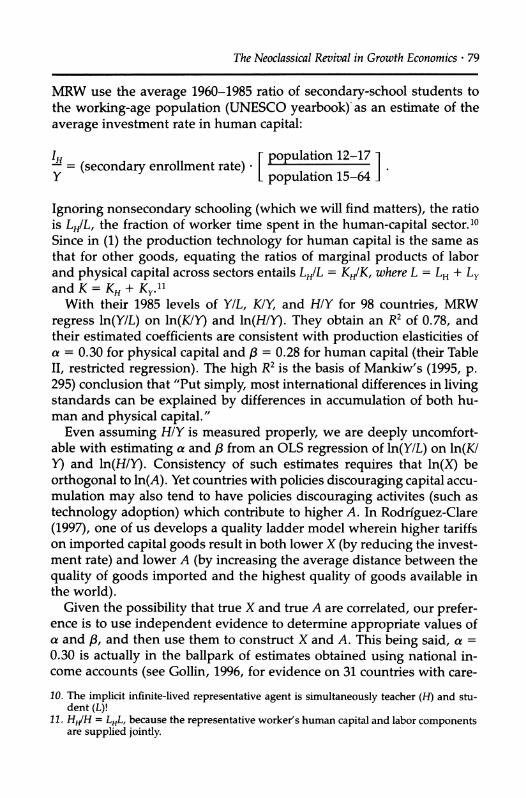
MRW use the average 1960-1985 ratio of secondary-school students to the working-age population (UNESCO yearbook) as an estimate of the

average investment rate in human capital:

IH L population 12-17 = (secondary enrollment rate) population 15-64 Y - Lpopulation 15-64

Ignoring nonsecondary schooling (which we will find matters), the ratio is LHIL, the fraction of worker time spent in the human-capital sector.'0 Since in (1) the production technology for human capital is the same as that for other goods, equating the ratios of marginal products of labor and physical capital across sectors entails LH/L = KH/K, where L = LH + Ly and K = KH+ Ky.l

With their 1985 levels of Y/L, K/Y, and H/Y for 98 countries, MRW

regress ln(Y/L) on ln(K/Y) and ln(H/Y). They obtain an R2 of 0.78, and their estimated coefficients are consistent with production elasticities of a = 0.30 for physical capital and /3 = 0.28 for human capital (their Table II, restricted regression). The high R2 is the basis of Mankiw's (1995, p. 295) conclusion that "Put simply, most international differences in living standards can be explained by differences in accumulation of both human and physical capital."

Even assuming H/Y is measured properly, we are deeply uncomfort- able with estimating a and 83 from an OLS regression of ln(Y/L) on ln(K/ Y) and ln(H/Y). Consistency of such estimates requires that ln(X) be orthogonal to ln(A). Yet countries with policies discouraging capital accumulation may also tend to have policies discouraging activites (such as technology adoption) which contribute to higher A. In Rodriguez-Clare (1997), one of us develops a quality ladder model wherein higher tariffs on imported capital goods result in both lower X (by reducing the investment rate) and lower A (by increasing the average distance between the quality of goods imported and the highest quality of goods available in the world).

Given the possibility that true X and true A are correlated, our prefer- ence is to use independent evidence to determine appropriate values of a and /, and then use them to construct X and A. This being said, a = 0.30 is actually in the ballpark of estimates obtained using national income accounts (see Gollin, 1996, for evidence on 31 countries with care-

10. The implicit infinite-lived representative agent is simultaneously teacher (H) and student (L)!

11. HHH = LHL, because the representative worker's human capital and labor components are supplied jointly.


ful treatment of proprietors' income). But we have no cause for comfort with p = 0.28. Studies such as Jorgenson (1995) and Young (1995) look at

compensation of workers in different education and experience categories, thereby bypassing the need to choose a single share going to human capital. In other words, the share going to labor input is 1 - a, and workers with more education and experience receive larger subshares of this 1 - a. We will do something similar in Section 3 below by looking at Mincerian estimates of wage differences across workers with different education and experience levels. For the rest of this section we keep f =

0.28, but we discuss at the end how the results are affected by consider-

ing higher values. We now show how the MRW results are sensitive to several modifica-

tions that we deem necessary. We keep a = 0.30 and P = 0.28 for com-

parison purposes. Given that our modified estimates of X and A will be correlated, there will not be a unique decomposition of the variance of

ln(Y/L) into the variance of ln(X) and the variance of ln(A).12 We think an informative way of characterizing the data is to split the covariance term, giving half to ln(X) and half to ln(A). This means we decompose the variance of ln(Y/L) as follows:

var ln(Y/L) cov(ln(Y/L),ln(Y/L)) cov(ln(Y/L),ln(X)) + cov(ln(Y/L),ln(A))

var ln(Y/L) var ln(Y/L) var ln(Y/L),

or

_cov(ln(Y/L),ln(X)) cov(ln(Y/L),ln(A)) 1= +

var ln(Y/L) var ln(Y/L)

This decomposition is equivalent to looking at the coefficients from inde-

pendently regressing ln(X) and ln(A), respectively, on ln(Y/L). Since

ln(X) + ln(A) = ln(Y/L) and OLS is a linear operator, the coefficients sum to one. So our decomposition amounts to asking, "When we see 1%

higher Y/L in one country relative to the mean of 98 countries, how much

higher is our conditional expectation of X and how much higher is our conditional expectation of A?" The first row of Table 1 gives the answer for MRWO, the original MRW measure. Since the covariance term is zero

by construction for MRWO, the breakdown is precisely their 78% ln(X) and 22% ln(A).

12. Since MRW construct ln(X) by regressing In(Y/L) on ln(H/Y) and ln(K/Y) with ln(A) as the residual, their ln(X) and ln(A) are orthogonal by construction, and the unique variance decomposition is R2, 1 - R2.


Table 1 THE ROLES OF A AND X IN 1985 PROSPERITYa

cov[ln(Y/L), In (Z)]/var ln(Y/L)

Sourcea Z= ( Z = Z = X Z=A

MRWO .29 .49 .78 .22 MRW1 .27 .49 .76 .24 MRW2 .31 .47 .78 .22 MRW3 .29 .11 .40 .60 MRW4 .29 .04 .33 .67

aMRWO: from MRW (uses their data appendix). MRW1: MRW0 but with Ky/Y instead of K/Y. MRW2: MRW1 but with L = worker instead of working-age population, 14 countries in/out. MRW3: MRW2 but with all enrollment rather than just secondary enrollment. MRW4: MRW3 but with (K, H, L) shares of (0.1, 0.4, 0.5), not (0.20, 0.28, 0.42), in H production.

Our first modification of MRW's methodology is to recognize that,

contrary to (1), national income accounting measures of output do not include the value of student time-an important component of human

capital investment.13 To see how important this might be, we consider the extreme case in which none of the human capital investment is measured as part of total output. To do this we replace K/Y and H/Y in

equation (2) with Ky/Y and Hy/Y, since only Ky and Hy are used in the

production of Y when Y does not include human capital investment. It turns out that the MRW measure of IH/Y, namely LHIL, is also appropriate for Hy/Y when all human capital investment goes unmeasured. The same is not true for physical capital intensity, for which we must use Ky/Y =

(KIY)(Ly/L). As shown by the MRW1 row of Table 1, this modification results in a 76% ln(X) vs. 24% ln(A) breakdown, so this distinction does not appear to be quantitatively important.

The MRW2 row of Table 1 reproduces the MRW1 row, only with up- dated data and a set of countries for which we have all the necessary schooling attainment data for the remainder of this paper. Like MRW,

13. MRW contend that this slippage between model and data is not quantitatively important. Parente and Prescott (1996) disagree, contending that unmeasured human capital investment must be implausibly large for the combined share of capital to be about two-thirds. Parente, Rogerson, and Wright (1996) illustrate that unmeasured investment would have to be 25-76% of GDP. We are in closer agreement with MRW, since, according to Kendrick (1976), about half of schooling investment consists of education expenditures (teachers, facilities) which are included in measured output. According to the 1996 Digest of Education Statistics published by the U.S. Department of Education (1996), education expenditures averaged 7% of GDP over 1960-1990. Back-of-the- envelope calculations suggest unmeasured investment might therefore be only 13% of GDP.


we have a sample of 98 countries.14 We use the latest Summers-Heston data (Mark 5.6) and use output per worker, whereas MRW used output per capita. The measure we use for Hy/Y here is the same as that used by MRW, except we use Barro and Lee's (1993) data on secondary enrollment rates in 1960, 1965, . . . , 1985 and United Nations (1994) population data by age groups to compute the value of

-= secondary enrollment rate population 15-19 Y population 15-64 J

for each country's investment rate in human capital in 1960, 1965, . ..

1985. MRW used population aged 12-17 in the numerator of the fraction in brackets, due to data availability. As shown in the MRW2 row of Table

1, if we see 1% higher Y/L, we expect 0.78% higher X and 0.22% higher A. Since the results are very similar to MRW1, we can now incorporate data on primary schooling enrollment, etc., for our sample of 98 countries without fear that the change in sample obscures the comparison.

Using data from Barro and Lee (1993), the MRW3 row of Table 1 uses

Hy/Y calculated with all three enrollment rates. The results are striking. Conditional on 1% higher Y/L in a country, we now expect only 0.40%

higher X and fully 0.60% higher A. As suggested by these results, primary enrollment rates do not vary as much across countries as secon-

dary enrollment rates do. The MRW3 measure of ln(Hy/Y) has only about

one-fourth the variance of the MRW0 measure of ln(Hy/Y).15 Moreover, the correlation of the MRW3 measure of ln(Hy/Y) with ln(Y/L) is only .52, as opposed to .84 for the MRW0 measure. This is not to say that primary-

schooling investments are unproductive compared to other schooling investments, for our methodology assumes that they are productive.16 It

14. In our sample but not in MRW's: Gambia, Guinea-Bissau, Lesotho, Swaziland, Barba- dos, Guyana, Iran, Iraq, Taiwan, Cyprus, Iceland, Malta, Yugoslavia, and Fiji. In MRW's sample but not in ours: Angola, Burkina Faso, Burundi, Chad, Egypt, Ethiopia, Ivory Coast, Madagascar, Mauritania, Morocco, Nigeria, Sierra Leone, Somalia, and Sudan.

15. One might think that adding primary schooling enrollment rates to secondary enrollment rates will not lower the variance, since adding a constant does not affect the variance of a random variable. But since we are looking at the percentage variance, adding the relatively stable primary school enrollment indeed lowers the variance.

16. In the next section we discuss Mincer regression evidence consistent with primary schooling indeed being productive. Specifically, each additional year of primary schooling in poor countries is associated with roughly 10% higher wages, suggesting important human capital investment is going on in primary schools that should not be ignored. There remains the issue of whether a year of enrollment in secondary school involves more investment in human capital than a year in primary school, so that the two enrollment rates should not simply be added together as we have done in the current section. The Mincer evidence that each additional year of schooling raises wages about 10% suggests that more absolute investment in human capital is occurring in secondary school than in primary school.


says, rather, that primary schooling does not vary anywhere near as much with Y/L across countries as secondary schooling does. By focus-

ing only on secondary schooling, one overstates the percentage variation in human capital across countries and its covariance with output per worker.

A further objection we have to the MRW measure of the human capital stock is that, as shown in (1), its construction assumes the same technol-

ogy for producing human capital as for producing consumption and

physical capital. Kendrick (1976) presents evidence that the technology for producing human capital is more intensive in labor than is the technology for producing other goods. He estimates that about 50% of investment in human capital in the-United States represents the opportunity cost of student time. The remaining 50% is composed of expenditures on teachers (human capital) and facilities (physical capital). According to the 1996 Digest of Education Statistics, expenditures on teachers represent about 80% of all expenditures. These figures suggest factor shares of 10%, 40%, and 50% for physical capital, human capital, and raw labor in the production of human capital, as opposed to the 30%, 28%, and 42% shares MRW use for the production of consumption goods and new

physical capital. If we let

IH = K --H (ALH) , (5)

this evidence suggests 4) = 0.4 and A = 0.5. Combining (2), (4), and (5) yields17

Hy ( L/ L \1/[1-K+A,I/(1-a-f3)] /K)[1-4- (1-fP)/(1-a-3)]/[1- +A3/(1-a-)()]

Y~L^-JI~~~~~ U~ ~(6) Y n+g+8 Y

When the two sectors have the same factor intensity (4) = 3 and A = 1 - a - 3), this reduces to Hy/Y = (LH/L)(n+g+8), which MRW used and we used above. But with ) = 0.40 and A = 0.50 the powers in (6) are 1.07 on the first fraction and -0.28 on the second. Because human capital production is more human capital-intensive than is the production of Y (0)>,3), a large share of labor devoted to human capital accumulation has a more than proportionate effect on Hy/Y. And because human capital production is less physical capital-intensive than is the production of Y (1 - 4 - A<a), a high rate of investment in physical capital raises Y more

17. Hy/Y = (Ly/L) (HIY) = (Ly/L) (IHIY)/(n+g+8) = [(Ly/L)/(n+g+8) (KH/Y)1'--A(HH/Y)t(ALH/ Y). The expression in the text can be obtained by substituting for A using (2) with Hy/Y and Ky/Y and by using KHIY = (LH/Ly) (Ky/Y) and HH/Y = (LH/Ly) (Hy/Y) (ignoring multiplicative constants).


than H, thereby reducing Hy/Y. As shown in the MRW4 row of Table 1, using ) = 0.40 and A = 0.50 results in a split of 33% ln(X) vs. 67% ln(A). Comparing MRW4 with MRW3, we see that lowering the capital inten-

sity of human capital production modestly lowers the variation of Hy/Y across countries.

As shown by comparing MRW0 with MRW4 in Table 1, the cumula- tive effect of these modifications is to remove the linchpin of the neoclassical revival: MRW's original (78%, 22%) decomposition has given way to a (33%, 67%) decomposition. Can one restore MRW's results with a

higher 3? Doubling 3 from 0.28 to 0.56 yields a (51%, 49%) division. As ,3 rises toward 23, the decomposition approaches 60% vs. 40%. Thus a

sufficiently high 3 does generate results that, although not as dramatic as those of MRW, still have the major part of international income variation explained by differences in levels of physical and human capital per worker. But what is the right value for 3? Unfortunately, we know of no independent estimates of "the" share of human capital. Fortunately, in the next section we are able to exploit wage regressions to measure human-capital stocks in a way that does not depend on the value of 3. This regression evidence also appropriately weights primary schooling attainment relative to secondary schooling attainment, rather than lumping them together with equal weight as we have done in the

preceding.

3. Using Mincer Regression Evidence to Estimate Human Capital Stocks

In this section we exploit evidence from the labor literature on the wage gains associated with more schooling and experience. For a cross section of workers, Mincer (1974) ran a regression of worker log wages on worker years of schooling and experience. He chose this specification because it fit the data much better than, say, a regression of the level of

wages on the years of schooling and experience. To incorporate this evidence into the technology for producing human capital, we abandon the infinite-life construct in favor of a life cycle in which people first go to school full time and then work full time. We specify the following tech-

nology for human capital:

h = (KH/LH)1 -

A(hT)(AeY/A)s)A, (7)

where hs is the human capital of somebody with s years of schooling, KH is the capital stock used in the education sector, LH is the number of

The Neoclassical Revival in Growth Economics ? 85

students, and hT is the human capital of each teacher. Manipulating (7) leads to18

Hy (/ \/[1-,+ A,3/(l-a-3)] (Ky)[l-,-A(l-3)/(1-a-3a)]/[-1 + A3/(1-a-f3)]

--^'M~~~~~ (7) <(8)

Bils and Klenow (1996) look at Mincer regression studies covering 48 countries and find that the wage gain associated with an additional year of education averages 9.5% across the 48 countries and ranges from 5% to 15% for 36 of the 48 countries. Based on technologies (1) and (7), the percentage wage gain to a representative agent from one more year of schooling is /8y/(1-a). Therefore, to match an estimated wage gain of 9.5% we set y = 0.095(1-a)/,3.

Table 2 presents results based on (7). The rows are labeled BKn because (7) is from Bils and Klenow (1996). As with MRW4 above, we use a = 0.30, f3 = 0.28, 4 = 0.4, and A = 0.5. For years of schooling s, row BK1 uses the level implied by the enrollment rates used in MRW3 and MRW4: s = 8 ? primary + 4 * secondary + 4 * tertiary. As the BK1 row shows, conditional on 1% higher Y/L we expect 0.60% higher X and 0.40% higher A. So switching from (6) used for MRW4 to (8) used for BK1 dramatically shifts the breakdown from (33%, 67%) to (60%, 40%). The exponential form of (7) implies that the higher the level of schooling, the bigger is the absolute amount of human capital obtained from the next year of schooling. The exponential form therefore puts more weight on secondary school enrollment than on primary school enrollment, moving us back toward MRW's 78%-vs.-22% breakdown.

One concern we have about BK1, as well as all of Table 1, is the assumption that in 1985 K/Y and H/Y are at steady-state levels. The data show lots of movement in country growth rates of Y, L, and YIL and in country investment rates in physical and human capital, suggesting that country K/Y and H/Y levels change over time. To estimate an off-steady- state 1985 K/Y, we use the accumulation equation and data on IIY and Y

18. In steady state h, = hT = h, so that the human capital of each student entering the workforce is the same as that of each teacher or worker. Using this fact, h = HHILH, so that H = hL = L(KH/ILH)1-~-A(HH/LH) (Ae(/)s)^, where HH is the total human capital of teachers. Expression (8) can then be obtained much as expression (6) was above. There are two (offsetting?) shortcomings in our treatment: First, we are assuming the student-teacher ratio is the same in each country (we fix it at one, but the level does not affect cross-country variance analysis). This ratio is presumably lower in richer countries. Second, our setup assumes that teacher education varies as much across countries as average worker education does (hT = h). In reality teacher schooling may vary less than average worker schooling, say if in every country high-school teachers must have at least a high-school diploma.


Table 2 THE ROLES OF A AND X IN 1985 PROSPERITY

cov[ln(Y/L), In (Z)]/var ln(Y/L)

Sourcea K

Z= ( Z = X Z =A

BK1 .29 .31 .60 .40 BK2 .23 .33 .56 .44 BK3 .23 .31 .53 .47 BK4 .23 .11 .34 .66

"BK1: uses (7), i.e. Mincer evidence. BK2: calculates years of schooling s from Barro-Lee 1985 stocks instead of 1960-1985 flows. BK3: adds average years of experience. BK4: BK3 but with (K, H, L) shares of (0, 0, 1) instead of (0.1, 0.4, 0.5) in H production.

over 1960-1985. Unfortunately, direct estimates of the 1960 K/Y are not available for most countries. We therefore set, for each country,

/K IK_ IK/Y J 196=g+8+n

with the investment rate IK/Y, the growth rate of YIL (g), and the population growth rate (n) equal to the country's averages over either 1960-1965, 1960-1970, or 1960-1985, and 8 either 0.03, 0.05, or 0.07. We also followed a procedure akin to King and Levine (1994) where we set g in the denomi- nator equal to a weighted average of own-country and world growth. The results were not at all sensitive to which way we calculated the 1960 K/Y, so we report the results with 1960 K/Y calculated using 8 = 0.03 (as in Table 1) and the country's own averages over 1960-1970 for g and n. To construct the 1985 H/Y, we use Barro and Lee's (1993) data on average years of

schooling attained by the 25-64-year-old population in each country in 1985. We report the results of using this approach to obtain 1985 levels of K/Y and H/Y in the BK2 row of Table 2. Conditional on 1% higher Y/L in one country in 1985, we expect 0.56% higher X and 0.44% higher A in that

country. These results are not far from the (60%, 40%) breakdown in BK1 with the steady-state assumption for K/Y and H/Y.19

We now modify (7) to incorporate human capital acquired through experience:

hs = (KH/LH) -- A(hT)4(Ae(ls+ Y2exp+ y3exp2)/) (9)

19. The close similarity between H/Y calculated in BK1 and in BK2, i.e. between school attainment implied by enrollments and measures of years of schooling attained, suggests that differences in the duration of primary, secondary, and higher education from our assumed 8, 4, and 4 years are not quantitatively meaningful.


where exp = (age - s - 6). The average experience level among workers was estimated using United Nations (1994) data in combination with Barro and Lee's schooling attainment data. For each country experience was calculated as the population-weighted average of (age - s - 6) at

ages 27, 32, . . ., 62 for the groups 25-29, 30-34, . ... , 60-64 in 1985.

Surprisingly, we find that the correlation between average years of experience of 25-64-year-olds and ln(Y/L) in 1985 is -0.67. Richer countries have older workforces, but slightly less experienced ones because they spend more years in school. As above, y, = 0.095(1-a)//3. Bils and Klenow (1996) report average estimated coefficients on exp and exp2 across 48 countries of 0.0495 and -0.0007. Based on these, we set 72 =

0.0495(1 -a)//3 and y3 = 0.0007(1 -a)c//. The consequence of adding experience can be seen in the BK3 row of Table 2. As compared to the (56%, 44%) split in BK2, the split in BK3 is (53%, 47%).

Underlying this breakdown of 53% ln(X) vs. 47% ln(A) is the supposi- tion that the quality of schooling is much higher in richer countries. In richer countries, students enjoy better facilities (higher KH/LH) and better teachers (higher HHILH). From (9), the quality of schooling is

quality of schooling = (KH/L-H)1 -h OAI .

Using this formula, for BK3 the elasticity of quality with respect to a country's Y/L is 0.95%.20 This means a country with 1% higher Y/L has 0.95% higher quality education. Note that higher quality of this type does not raise the percentage wage premium from education, but instead raises the base (log) wage for anyone in the country receiving some education. It should affect the intercept of the Mincer regression for a country, but not the coefficient on schooling.

Is an educational quality elasticity of 0.95% reasonable? Is it plausible that, like GDP per worker, the quality of education varies by a factor of about 34 across countries in 1985? An independent estimate of the quality elasticity can be gleaned from the wages of U.S. immigrants.21 Using 1970 and 1980 census data on the U.S. earnings of immigrants from 41 countries, Borjas (1987) estimates country-of-origin-specific intercepts in a Mincer regression of log wages on immigrant years of education and experience. He finds that immigrants with 1% higher per capita income in their country of origin exhibit a 0.116% higher wage intercept (stan-

20. Calculated as cov[ln(quality), ln(Y/L)]/var ln(Y/L). 21. Incidentally, the enormous pressure for migration from poor to rich countries is itself

consistent with substantial differences in productivity across countries. However, this pressure could be entirely explained by higher physical capital-output ratios and greater nonpecuniary benefits of living in richer countries.


dard error 0.025). This implies a quality elasticity of only 0.12%, suggesting that the elasticity embedded in BK3 is very aggressive.22'23

Borjas's evidence suggests an alternative, namely that teachers and class facilities affect school quality through the schooling coefficient y. In this event we would expect to see higher Mincer schooling coefficients in richer countries. Bils and Klenow (1996) find the opposite: each additional year of schooling brings roughly 10% higher wages in a

country where the average worker has 5 years of schooling, compared to only about 5% higher wages in a country where the average worker has 10 years of schooling. Perhaps 's are higher in richer countries, but the effect on the education premium is more than offset by a lower relative marginal product of human capital in richer countries. This could arise because of imperfect substitutability of workers with different education levels combined with abundance of human capital in richer countries. Indeed, the Cobb-Douglas technology in (1) implies unit elasticity of substitution between human capital and raw labor and therefore a falling education premium with a country's H/Y, holding y constant.

It is interesting to explore the possibility that the Mincer coefficients

already capture the effect of education quality combined with imperfect substitutability. This would correspond to the extreme case when teachers and class buildings affect only the /s, so that 4 = 0 and A = 1. It would be ideal to do this exercise using Mincer coefficients for each

country, but unfortunately we do not have such data for all countries. Here we use the average Mincer coefficient of 9.5% instead. (The reader should note that, since the Mincer coefficient is actually declining with income per worker, this biases the results against a large role for A.) As we report in the BK4 row of Table 2, without Mincer-intercept-type variations in school quality, human capital contributes much less to Y/L variation. The (ln(X), ln(A)) division shifts from (53%, 47%) in BK3 to

(34%, 66%) in BK4. How do we choose between BK3 and BK4? Recall that the school

22. Immigrants may be more able than the average person in their country of origin. Borjas's regression controls for observable differences in immigrants' ability such as age, years of schooling, and English proficiency. With regard to unobservables, the estimate of education quality differences would be biased downward if positive selection (in Borjas's terminology) were greater the poorer the country of origin. As Borjas notes, the opposite may be true, since income inequality tends to be greater in poorer countries.

23. Further cause for concern is the difficulty researchers such as Hanushek (1986) and Heckman, Layne-Farrar, and Todd (1996) have encountered in correlating schooling outcomes with teacher inputs. A (virtually controlled) experiment in Tennessee, however, found that the group of students placed in smaller K-3 classes performed significantly better on standardized tests (Mosteller, 1995).


quality elasticity implied by BK3 is 0.95%, whereas BK4 implies no variation in school quality (of the intercept type) across countries. The evidence from Borjas (1987) suggests that BK3's elasticity is much higher than the truth; the zero elasticity in BK4 seems closer. But if BK3 comes from data on the shares of capital and teachers in the U.S. education sector, why might it deliver wrong results? There are three possibilities. First is the reason we just gave, namely that these inputs affect the /s. Second, it could be that human capital varies much less across education sectors than across other sectors; i.e., international differences in human

capital may be smaller for teachers than for other workers. Finally, it could be that productivity A is not as significant in the education sector as it is in other sectors. In the extreme case when A does not enter the education sector at all, we find that the parameter values 4 = 0.19 and A = 0.81 generate a quality elasticity matching Borjas's 0.12. In this case we find a (42%, 58%) breakdown, in between BK3 and BK4 but a little closer to the latter.

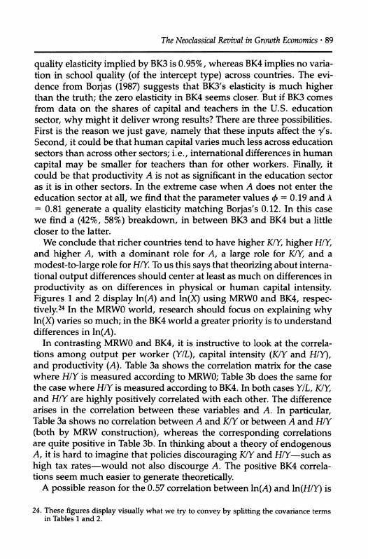
We conclude that richer countries tend to have higher K/Y, higher H/Y, and higher A, with a dominant role for A, a large role for K/Y, and a

modest-to-large role for H/Y. To us this says that theorizing about international output differences should center at least as much on differences in

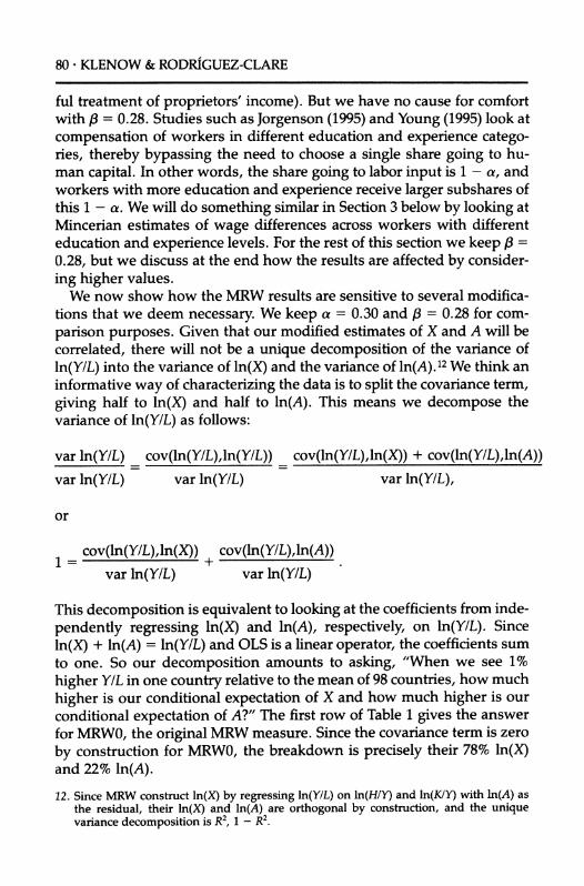
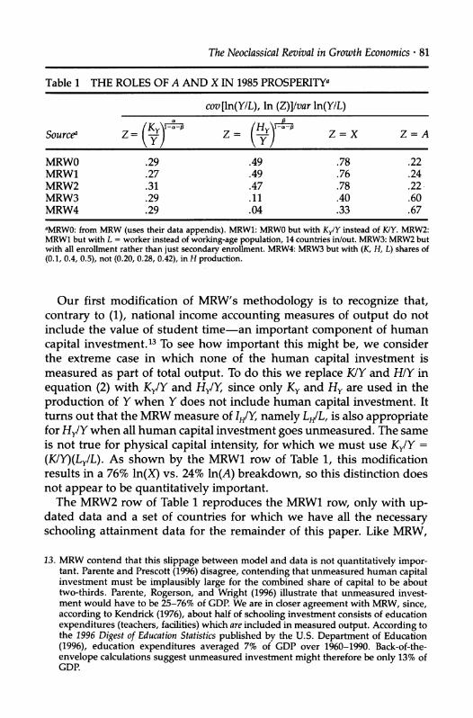
productivity as on differences in physical or human capital intensity. Figures 1 and 2 display ln(A) and ln(X) using MRWO and BK4, respectively.24 In the MRWO world, research should focus on explaining why ln(X) varies so much; in the BK4 world a greater priority is to understand differences in ln(A).

In contrasting MRWO and BK4, it is instructive to look at the correlations among output per worker (Y/L), capital intensity (K/Y and H/Y), and productivity (A). Table 3a shows the correlation matrix for the case where HIY is measured according to MRWO; Table 3b does the same for the case where H/Y is measured according to BK4. In both cases YIL, K/Y, and H/Y are highly positively correlated with each other. The difference arises in the correlation between these variables and A. In particular, Table 3a shows no correlation between A and K/Y or between A and H/Y (both by MRW construction), whereas the corresponding correlations are quite positive in Table 3b. In thinking about a theory of endogenous A, it is hard to imagine that policies discouraging K/Y and H/Y-such as high tax rates-would not also discourge A. The positive BK4 correlations seem much easier to generate theoretically.

A possible reason for the 0.57 correlation between ln(A) and ln(H/Y) is

24. These figures display visually what we try to convey by splitting the covariance terms in Tables 1 and 2.


Figure 1 1985 LEVELS: MRWO

2.0

1.5 -

1.0 -

* * * *

* *~

* * * *

-2.5 -2.0 -1.5 -1.0 -0.5 0.0

In(X)

0.5 1.0 1.5 2.0

that high H/Y, say due to generous education subsidies, facilitates tech-

nology adoption. Ciccone (1994) presents a model with this feature: the

larger the economy's stock of human capital, the more profitable it is for a firm to spend the fixed costs of adopting a given technology, and therefore the higher the economy's A relative to the world frontier. Note that this story links an economy's A to an economy's HIY, not an individual worker's A to an individual worker's h. We stress that the Mincer evidence deployed in this section should capture any link between the

schooling of an individual worker and the level of technology (e.g. equipment quality) that worker can use. This is because technology adoption that is linked to the individual should show up in the private wage gain to more education.

0.5

0.0 -

* t o *0

-0.5

-1.0

-1.5

-2.0

-2.5 ....I +

v


Figure 2 1985 LEVELS: BK4

1.5

1.0 -

0.5 - * *

**

* 4

.

0.0 -

C -0.5

*, * * **

* S* * * *' *

* - *% *2 *

* *

* * * *

*~~~ -1.0

-1.5 - ** *

-2.0 -1.0 -0.5 0.0 0.5 1.0 1.5

In(X)

Table 3 CORRELATION MATRICES

a. With MRWO methodology ln(Y/L) ln(KY) ln(H/Y)

ln(K/Y) .77 ln(H/Y) .84 .67 ln(A) .47 .00 .00

b. With BK4 Methodology ln(Y/L) ln(K/Y) ln(H/Y)

ln(K/Y) .59 ln(H/Y) .60 .02 ln(A) .93 .28 .57

-2.0 -1.5 I

,


At this point several robustness checks are in order. We first look at the potential importance of imperfect substitutability. For 45 countries in Bils and Klenow's (1996) sample, Barro and Lee (1996) report percentages of the 25-64-year-old population in seven educational attainment categories: none, some primary, completed primary only, some secondary, completed secondary only, some tertiary, and completed tertiary. We treat "some" as half-completed, and assume the durations are 8, 4, and 4 years for primary, secondary, and tertiary schooling. We assume the first three categories are perfectly substitutable "primary equivalents," and that the last four are perfectly substitutable "secondary equivalents":

Y = K(Hl-1/t Hl-1/1o)(1-a)/(1- lla) pnm sec /

with

Hpnm= E ALseY, Hs, = > ALAey,

s=0,4,8 s=10,12,14,16

where Ls is the number of working-age people in schooling group s. Note that this specification follows BK4 in eschewing Mincer-intercept- affecting school quality differences. We use nonlinear least squares to estimate or and y78/(1-a) using Barro and Lee's Ls data and Bils and Klenow's data on the estimated education premium for the 45 countries. The resulting estimates are y = 0.09(1-a)/f, and ar = 65.25 We then use these estimates to construct H aggregates for the 84 of our 98 countries for which Barro and Lee (1996) have the necessary schooling attainment data. The resulting breakdown is (40%, 60%), tilted a little toward ln(X) relative to the BK4 row, which uses y = 0.095(1- a)/l and ar = 1 (albeit with human capital vs. raw labor rather than primary equivalents vs.

secondary equivalents). We conclude from this exercise that allowing for

imperfect substitutability (and incorporating heterogeneity in schooling attainment within each country) does not significantly affect the results.

Our next robustness check concerns the size of f. In the previous section we found that raising the value of this parameter boosted the role of human capital in explaining international income variation. This does not happen here. Here we choose the coefficients y in (7) and (9) so that the implied wage gain for each additional year of education, which is

25. This degree of substitutability is very high compared to the 1.5 estimated by Katz and Murphy (1992) for high-school vs. college equivalents in the United States. We have imposed a common y, however, so our high estimated substitutability may be captur- ing the combination of less substitutability and higher y's in richer countries.


given by /3y/(l-a), matches the Mincer evidence discussed in Bils and Klenow (1996). Thus changing 3 results in an offsetting adjustment in y to preserve the equality 3y/(l-a) = 9.5%. In other words, there is no doubling of the importance of human capital from doubling f to 0.56, since the coefficient y must be halved at the same time. Indeed, there is zero effect. The intuition is that the Mincer estimates pin down the combined effect of translating schooling into human capital and translating human capital into output. Thus a larger elasticity of output with respect to human capital requires a smaller elasticity of human capital with respect to schooling in order to maintain consistency with the Mincer regression evidence.

An objection to the Mincer evidence is that the coefficient on schooling captures only private gains from schooling. Productive benefits of economywide human capital, as proposed by Lucas (1988), would be absorbed in the Mincer intercept. Lucas (1990) argues that human capital externalities can explain the large differences in TFP that Krueger (1968) found across 28 countries even after adjusting for human capital per worker (measured much as in BK4). Leaving aside the nature of these externalities, it is illuminating to ask how big they have to be in order to restore MRW's 78%-vs.-22% breakdown. For BK3, with its substantial variation in education quality, we find that the social Mincer coefficient on schooling would have to be 15.6%, as opposed to the 9.5% or so typically found. For BK4, the social education premium would have to be 29%. Since the evidence on school quality favors BK4, it appears that external benefits of schooling would need to be larger than the private benefits! In any case, entertaining externalities leads to questions about their exact nature and transmission. To us, this supports our call for more research into the source of productivity differences across countries.

4. From Development Accounting to Growth Accounting Whereas Tables 1 and 2 were concerned with development accounting (King and Levine's felicitous 1994 phrase), Table 4 is about growth accounting. For Table 4 we constructed K/Y and H/Y for each country in 1960 so that we could compute 1960-1985 growth rates. We did this for BK2 through BK4 (one cannot do it under the steady-state assumptions used for MRWs and for BK1). For H/Y we used Barro and Lee's (1993) schooling stocks in 1960 and, when necessary to construct experience levels, the United Nations (1994) population data for 1960. We estimated the 1960 Kl Y's as described in the previous section, and the results here are not at all sensitive to the various ways we tried to estimate 1960 K/Y's.

Table 4 presents the results of 1960-1985 growth accounting. When a


Table 4 THE ROLES OF A AND X IN 1960-1985 GROWTH

cov[A ln(Y/L), A In (Z)]/var A ln(Y/L)

Source Z= YZ Z = X Z = A

BK2 .03 .12 .15 .85 BK3 .03 .12 .14 .86 BK4 .03 .06 .09 .91

aBK2: calculates years of schooling s from Barro-Lee 1985 stocks instead of 1960-1985 flows. BK3: adds average years of experience. BK4: BK3 but with (K, H, L) shares of (0, 0, 1) instead of (0.1, 0.4, 0.5) in H production.

country's 1960-1985 growth rate of output per worker is 1% faster than

average, growth in physical capital intensity typically contributes about 0.03%. For BK2, which includes only the schooling contribution to human capital, H/Y growth contributes 0.12% more, the share owing to A

being 0.85%. Adding experience (BK3) does not change the calculus.

Letting education quality enter through the Mincer coefficients, as in BK4, boosts the contribution of A to 91%.

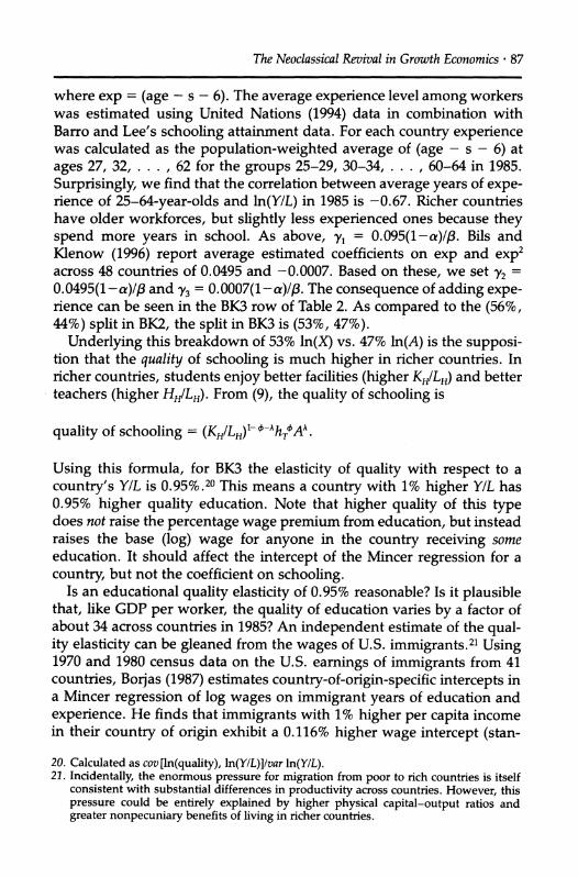
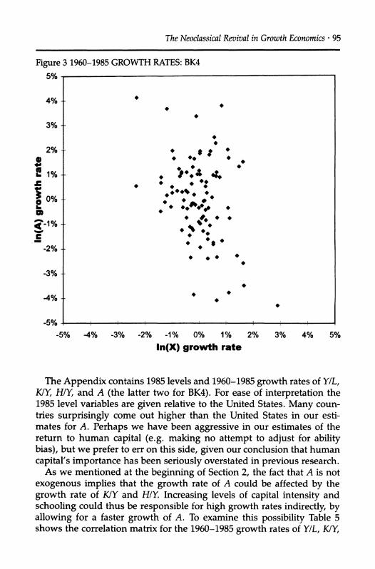
The consistent outcome in Table 4 is that differences in growth rates of Y/L derive overwhelmingly from differences in growth rates of A.26 Fig- ure 3 plots A growth against X growth (based on BK4) to demonstrate this visually. The small role we find for growth in the human-capital stock is not new. Benhabib and Spiegel (1994) and Pritchett (1995) report that the growth rate of schooling attainment is virtually uncorrelated with growth in output per worker across countries over 1960-1985. Barro and Sala-i-Martin find the same thing (1995, Chapter 12), but mark it down to measurement error.

Table 4 suggests that Chapters 1 to 4 in Barro and Sala-i-Martin (1995) and studies such as Chari, Kehoe, and McGrattan (1996) that emphasize transition dynamics of the neoclassical growth model ignore the major source of differences in country growth rates. Our results call for greater emphasis on models of technology diffusion and policies that directly affect productivity.27

26. For the 98-country sample, the unweighted average Y/L growth across the 98 countries is 2.24%. Using (2), this can be broken down into 0.77% from KIY growth, 0.44% from H/Y growth, and 1.03% from A growth. This average-world-growth accounting is distinct from the country-variation-in-growth-rates accounting that we focus on above. Unlike the country-variation-in-growth rates, which are dominated by variation in the growth rate of A, the trend growth in Y/L in the world (2.24%) owes more to X growth (1.21%) than to A growth (1.03%).

27. Some of the examples offered by Chari, Kehoe, and McGrattan (1996) as contributors to their effective tax rate may affect productivity A directly. Regulations and corruption would be expected to hinder firms' ability to translate K and H into Y.


Figure 3 1960-1985 GROWTH RATES: BK4

5%

4% -

2% -

E 1%

e 0%- . C

2%-

* *

#* *.* :t '

*

* A * . . ** *

-3% -

-5% -5% -4% -3% -2% -1% 0% 1% 2%

In(X) growth rate 3% 4% 5%

The Appendix contains 1985 levels and 1960-1985 growth rates of Y/L, KIY, HIY, and A (the latter two for BK4). For ease of interpretation the 1985 level variables are given relative to the United States. Many countries surprisingly come out higher than the United States in our estimates for A. Perhaps we have been aggressive in our estimates of the return to human capital (e.g. making no attempt to adjust for ability bias), but we prefer to err on this side, given our conclusion that human capital's importance has been seriously overstated in previous research.

As we mentioned at the beginning of Section 2, the fact that A is not exogenous implies that the growth rate of A could be affected by the growth rate of K/Y and H/Y. Increasing levels of capital intensity and schooling could thus be responsible for high growth rates indirectly, by allowing for a faster growth of A. To examine this possibility Table 5 shows the correlation matrix for the 1960-1985 growth rates of Y/L, K/Y,

i


Table 5 CORRELATION MATRIX (BK4 GROWTH RATES)

A ln(Y/L) A ln(K/Y) A ln(H/Y)

A ln(K/Y) .04 A ln(H/Y) .28 -.50 Aln(A) .87 -.42 .34

H/Y, and A according to BK4. The 0.34 correlation between the growth rates of A and H/Y suggests that countries with high growth in A have had unusually high growth rates of schooling. Thus it could be that high growth in economywide schooling attainment powerfully boosts growth through its effect on technology adoption. In contrast, the negative correlations between the growth rate of KIY and the growth rates of, respectively, H/Y and A are puzzling.28

An alternative way to think about the role of factor accumulation and total productivity factor (TFP) growth in explaining differences in economic performance across countries is to look at what has happened to the standard deviations of Y/L, KIY, H/Y, X, and A (as logarithms) across time. Table 6 compares the standard deviations of these variables in 1960 and 1985. As is well known, the standard deviation of the

logarithm of output per worker increased somewhat during this period (i.e., o-divergence). We find that o-convergence occurred for K/Y, but not for H/Y, X, and A. Thus the lack of a-convergence in Y/L does not stem from, say, A-convergence combined with X-divergence.29

5. Do Young's Findings Contradict Ours?

The debate over whether fast rates of growth in some countries stem from accumulation of capital or from technology catch-up has been heav-

ily influenced by the East Asian miracles. It was initially thought that these countries had very high TFP growth rates, pointing to technology catch-up as the heart of the story. Then came the careful work of Alwyn Young showing that these countries grew mostly through input accumulation (Young, 1995), and that their TFP growth rates were not extraordi-

narily high (Young, 1994). Singapore, for instance, was shown to have

28. The negative correlation between the growth rates of A and K/Y could indicate an overstatement of the contribution of K/Y to outut per worker. One reason for this may be that public investment (which is part of the data on investment that we used to

generate K/Y) is less efficient than private investment in generating efficiency units of capital. If this is true, then the role of A is even larger than shown in our results.

29. We also did our variance decomposition on the 1960 numbers and obtained exactly the same breakdown (34% ln(X) vs. 66% ln(A)) for BK4 that we did for 1985 in Table 2.


Table 6 STANDARD DEVIATIONS (BK4 LEVELS)

Quantity 1960 1985

ln(Y/L) 0.95 1.01 ln(K/Y) 0.73 0.55 ln(H/Y) 0.28 0.28 ln(X) 0.46 0.44 ln(A) 0.71 0.72

virtually no productivity growth over the last decades. As a result of this work, many people have concluded that the East Asian episodes illustrate the importance of neoclassical transition dynamics rather than technology catch-up.

We do not think this interpretation of Young's results is correct. First, as we argued above, we think the debate is over whether capital accumulation or technology catch-up explains growth in output per worker, not

growth in output. Neither hypothesis tries to explain the growth rate of

employment. Second, as we also argued above, growth in physical capital induced by rising productivity should be attributed to productivity [Barro and Sala-i-Martin also make this point (1995, p. 352)]. A higher level of productivity raises the marginal point of capital, thereby stimulat- ing investment and capital accumulation that would not have occurred without the higher level of productivity. The role of capital accumulation over and above that stimulated by productivity growth can be measured by the growth rate of the capital-output ratio. Table 7a reports a few calculations from Young's (1995) tables to illustrate the quantitative importance of these considerations. The annual growth rates of output and TFP, respectively, were 7.3% and 2.3% in Hong Kong, 8.7% and 0.2% in Singa- pore, 10.3% and 1.7% in South Korea, and 9.4% and 2.6% in Taiwan. So growth in output clearly came primarily from input accumulation. But the growth rates of output per worker and adjusted TFP-TFP raised to 1/ (1 - capital's share) because of its effect on capital accumulation-were as follows: 4.7% and 3.7% in Hong Kong, 4.2% and 0.3% in Singapore, 4.9% and 2.5% in South Korea, and 4.8% and 3.5% in Taiwan. So in three of the four East Asian miracles growth in output per worker came mostly from productivity gains.

In any case, the debate should not focus entirely on the miracle countries of East Asia. Although our data is much less detailed than the data Young compiled for each of the four Asian tigers, our hope is that by covering 98 countries we get a sense of whether Young's results are typi- cal of the sources of growth differences in the world as a whole. We are particularly interested, therefore, in whether our results for the Asian


Table 7

a. Alwyn Young's results

Country Y Growth TFP Growth

Hong Kong 7.3 2.3 Korea 10.3 1.7 Singapore 8.7 0.2 Taiwan 9.4 2.6

Country Y/L Growth A Growth

Hong Kong 4.7 3.7 Korea 4.9 2.5 Singapore 4.2 0.3 Taiwan 4.8 3.5

b. Young's A growth vs. ours

A growth

Country Young's Ours Why different?

Hong Kong 3.7 4.4 L data Korea 2.5 2.5 O.K. Singapore 0.3 3.3 L data; K share Taiwan 3.5 3.0 O.K.

tigers are not too far off from Young's numbers. Table 7b reports our BK4 1960-1985 A growth rates for the Asian tigers alongside Young's estimates. Our estimate for South Korea matches Young's (2.5%), and our estimate for Taiwan actually falls below Young's (3.0% vs. his 3.5%). For

Hong Kong our estimate is higher (4.4% vs. 3.7%), and for Singapore our estimate is much higher (3.3% vs. 0.3%). Young uses census data for L rather than Summers-Heston data, and the census data show faster

growth of L for Hong Kong and Singapore.30 Faster growth of L trans- lates into slower growth of Y/L and A (with growth in H/Y and K/Y

unaffected). This explains the entire difference in our estimates for Hong Kong. For Singapore Young used a physical-capital share of 0.49, as

opposed to the 0.30 we used. Combined with the difference in L growth, Young's higher capital share explains almost all of the gap in our Singa- pore estimates, since K/Y grew sharply there.

We close by stressing that our results share two important features

30. For 1966-1990, Young's worker/population ratios rose from 0.38 to 0.49 for Hong Kong and from 0.27 to 0.51 for Singapore. The comparable Summers-Heston figures were 0.54 to 0.65 and 0.34 to 0.48.


with those of Young (1994, 1995). First, we find a very modest role for

growth in human capital per worker in explaining growth (Young's ad- justments for labor quality are a few tenths of a percent per year). Sec- ond, we find that TFP growth accounts for most of the growth of output per worker in Hong Kong, South Korea, and Taiwan. And we stress that this relative importance of TFP growth for three of the four Asian tigers generalizes to our sample of 98 countries: we find that roughly 90% of

country differences in YIL growth are attributable to differences in A

growth. Combining these growth results with our findings on levels, we call for returning productivity differences to the center of theorizing about international differences in output per worker.

Appendix. Data

Y/L = 1985 RGDPW in Summers-Heston PWT 5.6. K/Y = 1985 physical-capital-to-output ratio (see Section 4 for K/Y used for BK2- BK4). H/Y = 1985 human-capital-to-output ratio (see Section 4 for H/Y used for BK4). A = 1985 level of productivity [see equation (2)]. Note: Levels are relative to the United States. g(Z) = 1960-1985 annual growth rate of series Z.

g(Y/L) g(K/Y) g(H/Y) g(A) Y/L KIY H/Y A (%) (%) (%) (%)

Algeria 0.40 0.79 0.33 0.99 2.89 0.71 0.64 1.96 Benin 0.07 0.47 0.34 0.25 0.78 1.37 0.02 -0.21 Botswana 0.20 0.49 0.47 0.55 6.85 2.20 0.71 4.81 Cameroon 0.11 0.27 0.56 0.43 4.22 1.16 0.63 2.97 Central Afr.R. 0.04 0.60 0.30 0.12 0.33 -0.79 0.53 0.54 Congo 0.20 0.29 0.48 0.81 4.06 -1.81 0.30 5.16 Gambia 0.05 0.39 0.38 0.18 1.37 4.32 -0.70 -1.25 Ghana 0.07 0.43 0.47 0.20 0.36 -0.60 1.51 -0.22 Guinea-Biss 0.04 1.23 0.22 0.10 1.52 -0.01 0.34 1.29 Kenya 0.06 0.63 0.40 0.15 1.31 -0.10 1.03 0.70 Lesotho 0.06 0.41 0.51 0.18 5.03 4.28 -0.55 2.34 Liberia 0.07 0.74 0.31 0.18 1.22 -0.82 0.92 1.19 Malawi 0.03 0.57 0.39 0.10 1.70 1.87 0.04 0.34 Mali 0.05 0.67 0.27 0.16 0.45 -2.28 0.77 1.57 Mauritius 0.22 0.42 0.57 0.59 0.90 -1.09 1.43 0.72 Mozambique 0.04 0.18 0.52 0.22 -1.18 2.98 -0.39 -3.05 Niger 0.03 0.79 0.25 0.10 0.79 1.82 -0.64 -0.09 Rwanda 0.05 0.18 0.55 0.23 1.89 1.70 -0.02 0.68 Senegal 0.08 0.38 0.45 0.27 0.87 -0.64 0.62 0.92 South Africa 0.29 0.84 0.45 0.57 1.82 1.23 0.12 0.86

100 - KLENOW & RODRIGUEZ-CLARE

g(YIL) g(K/Y) g(H/Y) g(A) Y/L K/Y H/Y A (%) (%) (%) (%)

Swaziland 0.15 0.53 0.47 0.41 2.96 2.87 0.35 0.67 Tanzania 0.03 0.59 0.37 0.08 2.08 1.80 0.05 0.77 Togo 0.04 0.76 0.32 0.12 2.60 3.02 0.28 0.26 Tunisia 0.26 0.46 0.42 0.81 3.22 -0.94 1.35 2.99 Uganda 0.04 0.19 0.57 0.17 0.06 0.96 0.17 -0.74 Zaire 0.03 0.24 0.54 0.14 0.42 4.19 -0.19 -2.45 Zambia 0.07 1.31 0.34 0.12 -0.42 -0.07 1.43 -1.32 Zimbabwe 0.10 0.61 0.38 0.26 1.50 -0.96 0.74 1.70

Barbados 0.36 0.51 0.77 0.70 2.39 1.55 0.46 0.97 Canada 0.92 0.97 0.85 1.05 1.88 0.64 0.94 0.80 Costa Rica 0.27 0.50 0.58 0.64 1.17 1.68 0.50 -0.36 Dominican Rep. 0.21 0.48 0.51 0.55 2.16 2.33 0.33 0.28 El Salvador 0.16 0.42 0.51 0.48 0.95 1.94 0.53 -0.79 Guatemala 0.22 0.54 0.40 0.62 1.32 1.24 0.47 0.12 Haiti 0.06 0.42 0.39 0.22 0.96 2.23 -0.07 -0.58 Honduras 0.14 0.50 0.46 0.38 1.41 0.21 0.93 0.64 Jamaica 0.14 0.93 0.39 0.28 0.34 1.23 0.56 -0.91 Mexico 0.50 0.49 0.53 1.29 2.33 1.27 0.70 0.95

Nicaragua 0.17 0.51 0.47 0.47 0.56 2.35 0.28 -1.31 Panama 0.30 0.58 0.62 0.60 3.00 1.45 0.62 1.55 Trinidad & Tobago 0.76 0.54 0.66 1.55 1.65 1.57 0.52 0.18 United States 1.00 1.00 1.00 1.00 1.30 0.56 1.27 0.04

Argentina 0.44 1.11 0.51 0.64 1.11 1.38 0.57 -0.25 Bolivia 0.17 0.81 0.42 0.35 2.11 0.57 0.48 1.38 Brazil 0.32 0.70 0.40 0.77 2.73 0.32 0.36 2.26 Chile 0.29 0.91 0.53 0.47 0.44 0.73 0.52 -0.43 Colombia 0.27 0.53 0.51 0.68 2.10 0.33 0.84 1.31 Ecuador 0.28 0.67 0.53 0.58 3.07 0.78 1.12 1.77

Guyana 0.11 1.34 0.37 0.17 -1.80 1.58 -0.18 -2.82 Paraguay 0.18 0.42 0.58 0.50 2.23 2.10 0.09 0.67 Peru 0.24 0.70 0.54 0.47 1.02 1.45 1.05 -0.72 Uruguay 0.30 1.22 0.48 0.43 0.17 1.34 0.87 -1.36 Venezuela 0.54 0.74 0.49 1.07 -0.43 2.46 0.82 -2.74

Bangladesh 0.13 0.24 0.52 0.55 1.73 -1.11 0.90 1.92

Hong Kong 0.49 0.57 0.74 0.88 5.49 0.53 1.08 4.39 India 0.08 0.71 0.38 0.20 1.74 -0.70 1.07 1.53 Indonesia 0.13 0.59 0.45 0.32 3.89 1.88 0.95 1.91 Iran 0.41 0.73 0.39 0.97 1.29 3.35 0.68 -1.55

Iraq 0.47 0.58 0.41 1.26 0.85 5.70 0.05 -3.26 Israel 0.65 0.88 0.79 0.84 3.27 0.79 1.02 2.03

Japan 0.56 1.35 0.60 0.63 5.30 2.01 0.51 3.53 Jordan 0.46 0.34 0.61 1.39 5.00 2.34 0.95 2.69 Korea, Rep. 0.31 0.58 0.76 0.54 5.37 2.32 1.77 2.54


g(YIL) g(K/Y) g(H/Y) g(A) Y/L K/Y H/Y A (%) (%) (%) (%)

Malaysia 0.31 0.68 0.51 0.63 3.74 1.30 1.21 2.00 Myanmar 0.04 0.39 0.42 0.14 2.64 0.36 0.46 2.08 Nepal 0.07 0.35 0.38 0.27 2.25 1.36 0.09 1.21 Pakistan 0.13 0.48 0.38 0.40 2.96 -0.31 0.76 2.68 Philippines 0.13 0.53 0.66 0.26 1.41 2.18 0.76 -0.65

Singapore 0.53 0.93 0.41 1.03 5.11 2.40 0.16 3.29 Sri Lanka 0.17 0.35 0.69 0.45 1.87 0.63 0.84 0.85 Syria 0.51 0.37 0.56 1.52 4.42 0.97 1.35 2.83 Taiwan 0.38 0.51 0.73 0.75 5.30 1.76 1.52 3.03 Thailand 0.14 0.53 0.55 0.33 3.70 0.87 0.62 2.66

Austria 0.71 1.53 0.45 0.88 3.20 0.74 1.42 1.72 Belgium 0.81 1.43 0.64 0.84 2.59 0.63 0.73 1.65 Cyprus 0.41 1.11 0.54 0.58 4.12 0.49 1.33 2.88 Denmark 0.71 1.49 0.73 0.66 1.91 0.58 0.26 1.32 Finland 0.70 1.80 0.60 0.65 2.87 0.15 0.97 2.11 France 0.80 1.47 0.45 1.04 2.79 1.16 1.02 1.29 Germany, W. 0.81 1.85 0.53 0.79 2.69 0.51 0.30 2.12 Greece 0.48 1.25 0.50 0.65 4.60 1.41 0.94 2.97 Iceland 0.69 1.10 0.59 0.91 2.46 -0.42 1.20 1.95 Ireland 0.57 1.07 0.62 0.75 3.31 0.93 0.47 2.33

Italy 0.80 1.51 0.43 1.04 3.60 0.44 0.85 2.72 Malta 0.46 0.95 0.56 0.70 4.71 -1.08 1.18 4.69 Netherlands 0.85 1.28 0.61 0.98 2.05 0.68 1.45 0.59 Norway 0.85 1.49 0.73 0.79 2.80 0.18 2.35 1.10 Portugal 0.34 1.21 0.34 0.60 3.40 0.93 0.83 2.18

Spain 0.63 1.28 0.42 0.93 3.80 1.91 0.71 1.96 Sweden 0.78 1.54 0.65 0.77 1.69 0.57 0.77 0.77 Switzerland 0.88 2.03 0.55 0.80 1.57 1.03 0.86 0.26 Turkey 0.21 0.79 0.37 0.48 3.19 1.23 0.41 2.04 United Kingdom 0.68 1.23 0.64 0.79 1.77 0.21 0.38 1.37

Yugoslavia 0.34 1.52 0.48 0.41 3.97 1.44 1.25 2.11

Australia 0.86 1.33 0.74 0.85 1.63 0.46 0.48 0.98 Fiji 0.29 0.68 0.61 0.53 1.03 0.25 0.86 0.28 New Zealand 0.77 1.25 0.94 0.68 0.81 0.38 1.01 -0.14 Papua N. Guinea 0.10 1.08 0.26 0.23 1.59 2.77 -0.54 -0.03

REFERENCES

Barro, R. J., and J.-W. Lee. (1993). International comparisons of educational attainment. Journal of Monetary Economics 32(3):363-394.

,and . (1996). International measures of schooling years and schooling quality. American Economic Review, Papers and Proceedings 86(2): 218-223.

, and X. Sala-i-Martin. (1995). Economic Growth. New York: McGraw-Hill.


Benhabib, J., and M. M. Spiegel. (1994). The role of human capital in economic development: Evidence from aggregate cross-country data. Journal of Monetary Economics 34(2):143-174.

Bils, M., and P. J. Klenow. (1996). Does schooling cause growth or the other way around? University of Chicago. Mimeo.

Borjas, G. J. (1987). Self-selection and the earnings of immigrants. American Economic Review 77(4):531-553.

Bosworth, B., S. M. Collins, and Y. Chen. (1995). Accounting for differences in economic growth. Washington: Brookings Institution. Brookings Discussion Paper 115.

Chari, V. V., P. J. Kehoe, and E. R. McGrattan. (1996). The poverty of nations: A quantitative exploration. Cambridge, MA: National Bureau of Economic Re- search. NBER Working Paper 5414.

Ciccone, A. (1994). Human capital and technical progress: Stagnation, transition, and growth, University of California at Berkeley. Mimeo.

Gollin, D. (1996). Getting income shares right: Accounting for the self-employed. Williamstown, MA: Williams College. Mimeo.

Grossman, G. M., and E. Helpman. (1991). Innovation and Growth in the Global Economy. Cambridge, MA: The MIT Press.

Hall, R. E., and C. I. Jones. (1996). The productivity of nations. Cambridge, MA: National Bureau of Economic Research. NBER Working Paper 5812.

Hanushek, E. A. (1986). The economics of schooling: Production and efficiency in public schools. Journal of Economic Literature 24(September):1141-1177.

Heckman, J. J., A. Lyane-Farrar, and P Todd (1996). "Does money matter? The effect of school resources on student achievement and adult success." An examination of the earnings-quality relationship. In The Link between Schools, Student Achievement, and Adult Success, Gary Burtless (ed.). Washington: Brook-

ings Institution, 192-289. Jorgenson, D. W. (1995). Productivity: Volume 1, Postwar U.S. Economic Growth.

Cambridge, MA: The MIT Press. Katz, L. E, and K. M. Murphy. (1992). Changes in relative wages, 1963-1997:

Supply and demand factors. Quarterly Journal of Economics 107(1):35-78. Kendrick, J. W. (1976). The Formation and Stocks of Total Capital. New York: Colum-

bia University Press for the NBER. King, R. G., and R. Levine. (1994). "Capital Fundamentalism, Economic Develop-

ment, and Economic Growth." Carnegie-Rochester Conference Series on Public

Policy 40:259-92. Krueger, A. 0. (1968). Factor endowments and per capital income differences

among countries. Economic Journal 78(311):641-659. Lucas, R. E. (1988). On the mechanics of economic development. Journal of

Monetary Economics 22(1):3-42. . (1990). Why doesn't capital flow from poor to rich countries? American

Economic Review 80(2):92-96. Mankiw, N. G., (1995). The growth of nations. In Brookings Papers on Economic

Activity, G. Perry and W. Brainard (eds.). Washington: Brookings Institution, Vol. 1, pp. 275-326.

, D. Romer, and D. N. Weil (1992). A contribution to the empirics of economic growth. Quarterly Journal of Economics 107(2):407-437.

Mincer, J. (1974). Schooling, Experience, and Earnings. New York: Columbia Univer- sity Press.

Comment 103

Mosteller, F (1995). The Tennessee study of class size in the early school grades. The Future of Children 5(2):113-127.

Parente, S., and E. C. Prescott. (1996). The barriers to riches. Philadelphia: Uni- versity of Pennsylvania; University of Minnesota. Manuscript.

,R. Rogerson, and R. Wright. (1996). Homework in development economics: Household production and the wealth of nations. Philadelphia: University of Pennsylvania. Mimeo.

Pritchett, L. (1995). Where has all the education gone? World Bank. Mimeo. Rodriguez-Clare, A. (1997). The role of trade in technology diffusion. University

of Chicago. Mimeo. Romer, P. M. (1990). Endogenous technological change. Journal of Political Econ-

omy 98(5):S71-S102. . (1993). Idea gaps and object gaps in economic development. Journal of

Monetary Economics 32(3):543-573. Summers, R., and A. Heston. (1991). The Penn World Table (Mark 5): An ex-

panded set of international comparisons, 1950-1988. Quarterly Journal of Eco- nomics 106(2):327-368. Mark 5.6 (an update) is available at nber.harvard.edu.

Stokey, N. L. (1991). Human capital, product quality, and growth. Quarterly Journal of Economics 106(2):587-617.

United Nations. (1994). The Sex and Age Distribution of the World Populations, the 1994 Revision. New York: United Nations.

U.S. Department of Education. (1996). 1996 Digest of Education Statistics. Washing- ton: U.S. Government Printing Office.

Young, A. (1991). Learning by doing and the dynamic effects of international trade. Quarterly Journal of Economics 106(2):369-406.

. (1994). Lessons from the East Asian NICs: A contrarian view. European Economic Review 38(3-4):964-973.

. (1995). The tyranny of numbers: Confronting the statistical realities of the east Asian growth experience. Quarterly Journal of Economics 110(3):641-680.

Comment N. GREGORY MANKIW Harvard University

Instructors of macroeconomics who teach their students about economic growth often use Solow's version of the neoclassical growth model as the starting point for discussion. This model shows very simply how an economy's production technology and its rates of capital accumulation determine its steady-state level of income per person. After presenting this elegant theory, the instructor is left with a nagging question: So what? Does this model really explain why some countries are rich and others are poor? Or does this model leave most of the action unexplained in a variable that has been called, at various times, total factor productivity, the Solow residual, and "a measure of our ignorance"?

Comment 103

Mosteller, F (1995). The Tennessee study of class size in the early school grades. The Future of Children 5(2):113-127.

Parente, S., and E. C. Prescott. (1996). The barriers to riches. Philadelphia: Uni- versity of Pennsylvania; University of Minnesota. Manuscript.

,R. Rogerson, and R. Wright. (1996). Homework in development economics: Household production and the wealth of nations. Philadelphia: University of Pennsylvania. Mimeo.

Pritchett, L. (1995). Where has all the education gone? World Bank. Mimeo. Rodriguez-Clare, A. (1997). The role of trade in technology diffusion. University

of Chicago. Mimeo. Romer, P. M. (1990). Endogenous technological change. Journal of Political Econ-

omy 98(5):S71-S102. . (1993). Idea gaps and object gaps in economic development. Journal of

Monetary Economics 32(3):543-573. Summers, R., and A. Heston. (1991). The Penn World Table (Mark 5): An ex-

panded set of international comparisons, 1950-1988. Quarterly Journal of Eco- nomics 106(2):327-368. Mark 5.6 (an update) is available at nber.harvard.edu.

Stokey, N. L. (1991). Human capital, product quality, and growth. Quarterly Journal of Economics 106(2):587-617.

United Nations. (1994). The Sex and Age Distribution of the World Populations, the 1994 Revision. New York: United Nations.

U.S. Department of Education. (1996). 1996 Digest of Education Statistics. Washing- ton: U.S. Government Printing Office.

Young, A. (1991). Learning by doing and the dynamic effects of international trade. Quarterly Journal of Economics 106(2):369-406.

. (1994). Lessons from the East Asian NICs: A contrarian view. European Economic Review 38(3-4):964-973.

. (1995). The tyranny of numbers: Confronting the statistical realities of the east Asian growth experience. Quarterly Journal of Economics 110(3):641-680.

Comment N. GREGORY MANKIW Harvard University

Instructors of macroeconomics who teach their students about economic growth often use Solow's version of the neoclassical growth model as the starting point for discussion. This model shows very simply how an economy's production technology and its rates of capital accumulation determine its steady-state level of income per person. After presenting this elegant theory, the instructor is left with a nagging question: So what? Does this model really explain why some countries are rich and others are poor? Or does this model leave most of the action unexplained in a variable that has been called, at various times, total factor productivity, the Solow residual, and "a measure of our ignorance"?

104 * MANKIW

Several years ago, David Romer, David Weil, and I took a stab at

answering this question using the rightly famous Summers-Heston data- set. At one point in our paper, we offered an ordinary-least-squares regression of income per person on the investment rate and the population growth rate-two variables that determine an economy's steady state according to the most basic Solow model. These variables entered the regression with the signs that the theory predicts, and the R2 was 0.59. When we added a crude proxy for human-capital accumulation to the regression, the signs of the coefficients remained consistent with the

theory, and the R2 rose to 0.78. This large R2 surprised us, in part because these international data are surely subject to measurement error, which tends to bias the R2 downward. Our measure of human-capital accumulation was particularly crude. Given this bias, therefore, we took the high R2 as evidence that there may be a good deal of truth to the basic neoclassical growth model.

The weak link in our paper-and, I would argue, in most of the

empirical literature on economic growth-is the identification problem. Correlation does not imply causation, even in the Summers-Heston data. A high R2 in a regression cannot establish, for instance, whether a

high investment rate causes a high level of income (as the Solow model

predicts) or vice versa. Nonetheless, I have always found the high R2

reassuring when I teach the Solow growth model. Surely, a low R2 in this

regression would have shaken my faith that this model has much to teach us about international differences in income.

This paper by Klenow and Rodriguez tries to cast doubt on the conclusion we reached, but surprisingly it does not do so by attacking our weak link. Discussion of the identification problem is largely absent from this paper. Instead, the paper points out-completely correctly-that our measure of human-capital accumulation was very crude. If only we had used a better measure of human capital, they argue, we would have reached a different conclusion. In particular, they claim that with a better measure of human capital, we would have concluded that the neoclassical growth model explains only a small fraction of international differences in income.

At first glance, this conclusion seems odd. A standard result in econo- metrics is that measurement error reduces an equation's explanatory power. Adding additional information should always improve an equation's fit. How is it that Klenow and Rodriguez explain less than we did

by bringing more information to bear on the problem? The answer lies at the heart of this paper.

Klenow and Rodriguez employ an empirical strategy that is fundamen-

tally different from that used in my paper with Romer and Weil. Our

Comment* 105

approach was one of estimation. That is, we used ordinary least squares to find the parameters that best fit the cross-country data and then asked whether these estimated parameters made sense in the context of a Solow growth model augmented to include human as well has physical capital. By allowing the data to choose the parameters, we were in es- sence allowing the model to take its best shot. By contrast, Klenow and Rodriguez adopt an approach that is more similar to growth accounting. In particular, they calibrate the key parameters and then see how much human- and physical-capital accumulation can explain, given those parameter values.

Their results are necessarily sensitive to the particular parameters they choose. Unfortunately, these are not parameters about which anyone can be greatly confident. These authors begin in their Table 1 with a Cobb-Douglas production function with physical capital, human capital, and raw labor. It is straightfoward to calculate the sensitivity of these results. The amount of international income variation attributed to human capital in this table is simply proportional to /3(1 - a - 3). Klenow and Rodriguez use a = 0.30 and 3 = 0.28, which makes //(1 - a - 3) = 0.67. Yet if we assume instead that a = 0.35 and 3 = 0.50, then //(1 - a - /) = 3.33. In this case, the role of human capital in explaining international income differences is 5 times larger than what is presented in Table 1. I am not raising this issue because I know that the parameters a = 0.35 and /3 = 0.50 are better than the parameters Klenow and Rodri- guez use. Rather, I am suggesting that we don't really know what the right parameters are with much precision, and that many of the results in this paper presume that we do.

A related issue is how we combine human-capital accumulation at different levels of schooling. Romer, Weil, and I used data for secondary schooling. By contrast, this paper takes the very sensible approach of combining the secondary-school data with data on primary-school and higher education. (The more important addition here is the primary- school data. Higher education is so small in so many countries that variation in it matters much less in this paper's calculations.) Klenow and Rodriguez combine these various data to produce a single summary measure of human-capital accumulation.

Before reading this paper, I would have expected that Klenow and Rodriguez's measure of schooling would be better than the one we used. Yet, in fact, their new measure does a worse job of explaining cross- country differences in income. They report that their sophisticated human-capital measure has a correlation with income of only 0.52, while the cruder measure that ignores the primary-school data has a correlation with income of 0.84.

106 * MANKIW

How could this be? Why is the crude measure of human capital more correlated with income than the sophisticated measure? One possibility is that the sophisticated measure is not really better than the crude measure. I can think of various reasons why this might be the case.

When combining different enrollment rates, it is natural to produce a measure something like average years of schooling. This standard approach implicitly assumes, however, that a year of schooling for a 7-year- old produces as much human capital as a year of schooling for a 15-year- old. This assumption may not be right. Certainly, both students make the same contribution to the society's total years of schooling. Yet one

might argue that a year of schooling for a 15-year-old in fact contributes more to the stock of human capital. A natural measure of the human-

capital stock is its opportunity cost-that is, the output that has been

forgone as students are put through school. Because the market wage of a 15-year-old is much higher than the market wage of a 7-year-old, the cost of a year of secondary schooling is much greater than that of a year of primary schooling. From this perspective, it is plausible to give greater weight to secondary enrollment rates than primary enrollment rates when computing the aggregate accumulation of human capital.

It is also worth considering what students are doing when they are not in school. A 15-year-old who is not at school is presumably working at a

job. Thus, secondary-school enrollment represents the decision between work and education. By contrast, a 7-year-old not at school might be at home with a parent. This time may at least partly represent a form of home schooling. If so, international differences in primary-school enrollment might contain little information about human-capital accumulation.

A clear example of this phenomenon is the rise of day care in the United States. Many 2-, 3-, and 4-year-olds now attend organized day-care cen- ters rather than staying at home with a parent as they did in the past. Should we say that this change represents an increase in human-capital accumulation, or merely a change in child-care arrangement? Probably the latter. But perhaps the same argument applies to 7-year-olds. If one

society chooses to keep 7-year-olds at home with one-on-one attention from parents, while another society sends them to primary schools with classes of forty students and one teacher, we should not be so quick to say that the first society is deficient in human-capital accumulation.

Another reason we might want to give greater weight to secondary schooling than to primary schooling involves externalities. The idea that human capital generates positive externalities appears in many recent discussions of economic growth and is, in my view, very appealing. It

explains, for instance, why all countries choose to subsidize education,

Comment 107

why developing countries are concerned about the brain drain, and why good students prefer to be at schools with other good students. Once we start thinking about externalities, it seems unlikely that they are the same at all levels of schooling. One externality often mentioned is that educated people generate good ideas that enter society's pool of knowl-

edge. This externality might well flow largely from the most educated members of society. If so, differences in secondary and higher education would be more important than differences in primary education.

I should note that an important semantic issue arises here. When Klenow and Rodriguez calibrate their model, they do so using the private return to schooling. In their view, externalities from human capital are outside the realm of the neoclassical model; if such externalities are

important, that calls into doubt the neoclassical revival. A broader view of the neoclassical growth model, however, is that it emphasizes capital accumulation as the key to growth, and it can potentially allow for such externalities. Certainly, that is the view I have taken when defending the neoclassical model as a useful theory of international differences in liv-

ing standards. All of the issues I have raised point to a single conclusion: We don't

know as much as we need to know to calibrate the contribution of human capital to the production process. In particular, we don't know with much precision the share of income that accrues to human capital, we don't know what weight to attach to various levels of education when measuring the total stock of human capital, and we don't know the social return to a year of schooling. In the end, therefore, I am not convinced by this paper's central conclusion that human and physical capital are incapable of explaining the bulk of international differences in income. Put simply, this conclusion is based on more assumptions about unknown parameters than I am willing to swallow.

Comment CHARLES I. JONES Stanford University

1. Introduction

The neoclassical growth revival is associated with the hypothesis that most of the variation in levels of per capita income across countries is associated with variation in capital and skills, and most of the variation

Comment 107

why developing countries are concerned about the brain drain, and why good students prefer to be at schools with other good students. Once we start thinking about externalities, it seems unlikely that they are the same at all levels of schooling. One externality often mentioned is that educated people generate good ideas that enter society's pool of knowl-

edge. This externality might well flow largely from the most educated members of society. If so, differences in secondary and higher education would be more important than differences in primary education.

I should note that an important semantic issue arises here. When Klenow and Rodriguez calibrate their model, they do so using the private return to schooling. In their view, externalities from human capital are outside the realm of the neoclassical model; if such externalities are

important, that calls into doubt the neoclassical revival. A broader view of the neoclassical growth model, however, is that it emphasizes capital accumulation as the key to growth, and it can potentially allow for such externalities. Certainly, that is the view I have taken when defending the neoclassical model as a useful theory of international differences in liv-

ing standards. All of the issues I have raised point to a single conclusion: We don't

know as much as we need to know to calibrate the contribution of human capital to the production process. In particular, we don't know with much precision the share of income that accrues to human capital, we don't know what weight to attach to various levels of education when measuring the total stock of human capital, and we don't know the social return to a year of schooling. In the end, therefore, I am not convinced by this paper's central conclusion that human and physical capital are incapable of explaining the bulk of international differences in income. Put simply, this conclusion is based on more assumptions about unknown parameters than I am willing to swallow.

Comment CHARLES I. JONES Stanford University

1. Introduction

The neoclassical growth revival is associated with the hypothesis that most of the variation in levels of per capita income across countries is associated with variation in capital and skills, and most of the variation

108 * JONES

in growth rates of per capita income across countries is associated with variation in the growth rate of capital and skills. Klenow and Rodriguez associate this view primarily with two papers-Mankiw, Romer, and Weil (1992) (MRW) and Young (1995)-but Mankiw (1995) summarizes this work and provides the clearest statement of the neoclassical growth revival.

Klenow and Rodriguez question both tenets of the neoclassical growth revival and argue that "the dominant cause of the large international

dispersion in levels and growth rates of output per worker" is differences in (multifactor) productivity. I do not find much to disagree with in this conclusion, except that it perhaps overemphasizes the importance of productivity. Indeed, Hall and I have argued elsewhere (Hall and Jones, 1996) that levels of productivity vary greatly across countries. We use a slightly different methodology-for example, we follow Solow (1957) in not making an assumption about the exact functional form of the production function-and reach the same conclusion. Part of the reason why the United States has a higher GDP per worker than Ethio-

pia is that the United States invests more in physical capital and its workers have a much higher level of education. However, a key part of the explanation is also that the United States uses its inputs much more

productively than does Ethiopia. My comments are divided into two parts. The first part attempts to

clarify some of the points made by Klenow and Rodriguez. In the process, I will argue that it is not obvious from the MRW evidence that there should have been a neoclassical revival in the first place. The second part steps back to consider where we are in our understanding of the differences in levels and growth rates of output per worker across countries.

2. Should There Have Been a Neoclassical Revival?

My first comment is related to interpreting the results in Klenow and

Rodriguez's Table 1, where they decompose differences in output per worker across countries into the contribution from productivity, A, and the contribution from inputs, X. Their summary statistics are based on the coefficients obtained from regressing log A on log y and log X on log y, where y denotes GDP per worker. They interpret these coefficients as conditional expectations: if GDP per worker is higher by one percent, what is our best guess as to how much higher productivity and inputs are?

These coefficients can be motivated in a different way. For example, one might be concerned with how much of the variation in output per

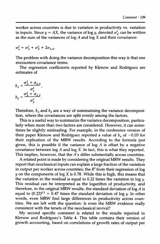
Comment. 109

worker across countries is due to variation in productivity vs. variation in inputs. Since y = AX, the variance of log y, denoted cr, can be written as the sum of the variances of log A and log X and their covariance:

_y = o' + crx + 2(A,x.

The problem with doing the variance decomposition this way is that one encounters covariance terms.

The regression coefficients reported by Klenow and Rodriguez are estimates of

2A + a,x _T, + A,X bA -

+ - X + QA,X

bx =

Therefore, bA and bx are a way of summarizing the variance decomposition, where the covariances are split evenly among the factors.

This is a useful way to summarize the variance decomposition, particularly when more than two factors are considered. However, it can some- times be slightly misleading. For example, in the conference version of their paper Klenow and Rodriguez reported a value of bA of -0.03 for their replication of the MRW results. According to the formula just given, this is possible if the variance of log A is offset by a negative covariance between log A and log X. In fact, this is what they reported. This implies, however, that the A's differ substantially across countries.

A related point is made by considering the original MRW results. They report that neoclassical inputs can explain a large fraction of the variation in output per worker across countries; the R2 from their regression of log y on the components of log X is 0.78. While this is high, this means that the variation in the residual is equal to 0.22 times the variation in log y. This residual can be interpreted as the logarithm of productivity, and therefore, in the original MRW results, the standard deviation of log A is equal to (0.22)?.5 = 0.47 times the standard deviation of log y. In other words, even MRW find large differences in productivity across countries. We are left with the question: Is even the MRW evidence really consistent with the tenets of the neoclassical revival?

My second specific comment is related to the results reported in Klenow and Rodriguez's Table 4. This table contains their version of growth accounting, based on correlations of growth rates of output per

110 * JONES

worker with growth rates in factor intensities. They infer from this exercise that most of the variation in growth rates across countries is the result of total factor productivity (TFP) growth rather than growth in the

inputs. I like the basic approach here, but I'd like to suggest an alternative. If

all countries were in their steady states, then, as is well known, all

growth would be attributable to TFP growth. In this sense, the KR meth-

odology is in some ways set up to deliver their result. An alternative way of gauging the relative importance of TFP growth in inputs that gets around this problem is to ask how much of the exceptional growth in

output per worker is due to exceptional productivity growth and exceptional capital deepening.

This exercise is carried out here using the data from Young (1995), as

reported by Klenow and Rodriguez. Specifically, I assume that the world's technological frontier is growing at an annual rate of 1%. This number is chosen for convenience; it is easy to see how other numbers would affect the results. Then the growth rate of output per worker can be written as the sum of the growth rate of the world technological frontier, plus the exceptional growth in A and the exceptional deepening (growth in X). According to the results shown here in Table 1, roughly half of the exceptional (i.e. faster than the world frontier) growth in the East Asian economies is due to exceptional growth in A and roughly half is due to exceptional growth in the intensity of the inputs. These results, together with the basic finding (documented in Table 2 of Klenow and

Rodriguez) that between 40% and 60% of the variation in levels is due to variation in A, lead me to conclude that roughly half of the variation in both levels and growth rates of output per worker is due to productivity. I think this is worth emphasizing, because oftentimes readers want an

all-or-nothing answer, and they may be tempted to conclude from Klenow and Rodriguez's paper that "everything is productivity." A better answer, I think, is that both traditional inputs and productivity play large and important roles.

Table 1 ACCOUNTING FOR MIRACLES

Growth Exceptional of world Exceptional A growth, deepening,

Country gYIL frontier (%) gA - 1% (%) gx (%)

Hong Kong 4.7 1 2.7 1.0

Singapore 4.2 1 -0.7 3.9 S. Korea 4.9 1 1.5 2.4 Taiwan 4.8 1 2.5 1.3

Comment 111

3. Our Current State of Knowledge

I want to end my comment with a discussion of the current state of our

knowledge about economic growth. One of the important goals of the

growth literature is to provide a formal characterization of the dynamic production possibilities of the economy, that is, to provide a model that

specifies an aggregate production function Y = F(K, H, L, A, . . . ) as well as how the inputs into production evolve over time.

Different papers in the growth literature characterize this dynamic PPF differently. For example, Solow's (1957) paper was concerned with

figuring out the "shape" of the aggregate production function F(.), since Solow (1956) recognized that the dynamics of the neoclassical growth model hinged on this function. MRW can also be read as trying to pin down the shape of the aggregate production function within the class of

Cobb-Douglas production functions. With hindsight, estimating the parameters of the aggregate produc-

tion function econometrically appears to be impossible. The required identifying assumption is that one can separate shifts of the production function from movements along the production function. In practice, I do not see how this can be done. For example, to use instrumental variables, one needs to find a variable that changes the capital stock without changing the efficiency with which the capital is used. In practice, anything that stimulates capital is likely to stimulate productivity as well, particularly if unmeasured utilization is a problem.

For this reason, I now have less confidence in modeling the aggregate production function as Y = K'13H'3(AL)113, as originally suggested by MRW. In addition, Klenow and Rodriguez claim that MRW are

using the wrong measure of human capital in their regression. Had they used Klenow and Rodriguez's data, presumably they would have estimated different exponents for the production function. Therefore, I see no evidence that the aggregate production function should take this form. Instead, one has to use other evidence such as the absence of trends in factor shares to try to restrict the shape of the production function.

An important contribution of Bils and Klenow (1996) is to argue that the Mincerian wage regressions in the labor literature provide a useful piece of evidence to match in modeling human capital. Like the absence of trends in factor shares, this independent evidence tells us something about the way educational attainment affects ouptut, and it seems to me that this is a superior way of characterizing the human capital portion of the dynamic production possibilities of the economy.

Based on these papers and on other work in the growth literature, one

112 * JONES

way to describe the dynamic production possibilities frontier of economies is

Y = AK(hL)l-, a =, K=Y-C-SK, h = eYS, A= ?

The first equation is an aggregate production function in which there is one type of labor in the economy with a skill level h determined by educational attainment. I've simplified the production function relative to Klenow and Rodriguez and MRW. In fact, workers with different skills are probably not perfect substitutes, and the evidence on changes in relative wages suggests that maybe technical change is skill-biased. However, at this point in time, I don't think there is a clear candidate

production function with these properties, and growth economists are

typically using aggregate measures of human capital that do not distin-

guish the skill levels of different workers anyway. I've left the modeling of A unspecified. For the growth of A, Romer

(1990), Grossman and Helpman (1991), and others have provided us with very nice theories.1 About the levels of A we know much less. To the extent that one associates productivity with ideas, models of technol-

ogy diffusion and transfer are relevant. However, it seems likely that differences in productivity reflect more than simply differences in tech-

nology; for example, Hall and Jones (1996) find that the U.S. level of

productivity ranks 11th out of 133 countries. A suggestive stylized fact documented both by Hall and Jones and by

Klenow and Rodriguez is that productivity and inputs are highly correlated across countries. Poor countries have low levels of education, investment, and productivity. Rich countries have high levels of inputs and productivity. This correlation suggests that common driving forces

may be at work. Hall and I document that measures of the extent to which the government policies and institutions of the economy discour-

age diversion and rent-seeking can explain much of this correlation and

provide a clear empirical explanation for why some countries are so much richer and more productive than others.

REFERENCES

Bils, M., and P. Klenow. (1996). Does schooling cause growth or the other way around? University of Chicago Graduate School of Business. Mimeo.

1. I, of course, prefer the versions of these models in which growth rates are not increasing in the size of the economy, as in Jones (1995).

Discussion ?113


Hall, R. E., and C. I. Jones (1996). The productivity of nations. Cambridge, MA: National Bureau of Economic Research. NBER Working Paper 5812. November.

Jones, C. I. (1995). R&D-based models of economic growth. Journal of Political Economy 103(August):759-784.

Mankiw, N. G. (1995). The growth of nations. Brookings Papers on Economic Activ- ity 1:275-326.

, D. Romer, and D. Weil. (1992). A contribution to the empirics of economic growth. Quarterly Journal of Economics 107(2, May):407-438.

Romer, P. M. (1990). Endogenous technological change. Journal of Political Econ- omy 98(5, October):S71-S102.

Solow, R. M. (1956). A contribution to the theory of economic growth. Quarterly Journal of Economics 70(February):65-94.

. (1957). Technical change and the aggregate production function, Review of Economics and Statistics 39(August 3):312-320.

Young, A. (1995). The tyranny of numbers: Confronting the statistical realities of the east Asian growth experience. Quarterly Journal of Economics 110(3):641-680.

Discussion

Robert King began the discussion by asking whether it is feasible to create a more comprehensive human-capital measure using measures of educational attainment available from the United Nations, then aggregat- ing using a reference wage rate. In particular, he noted that similar work has been done in the past by Anne Krueger, but that the data are probably of higher quality now.

Francesco Caselli observed that panel-data techniques developed to deal with omitted-variable bias may be used to identify differences in technology across countries. In his own work he has been able to estimate TFP directly instead of having to rely on the error term for its identification. His finding is that the direct estimates of TFP are highly variable across countries, supporting the conclusions of Klenow and Rodriguez.

Susanto Basu pointed out that the paper largely ignores issues of capital mismeasurement. He cited work by Jong-Wha Lee and others that attributes most of the growth benefits of openness to imports of capital goods. This result suggests that embodiment of technological advances in new capital is important to a degree that may not be captured very well in the Summers-Heston data.

John Haltiwanger expressed two reservations. First, he cited a paper by Baily, Hulten, and Campbell which used plant-level data to decompose aggregate productivity growth into its sources. Those authors

Discussion ?113


Hall, R. E., and C. I. Jones (1996). The productivity of nations. Cambridge, MA: National Bureau of Economic Research. NBER Working Paper 5812. November.

Jones, C. I. (1995). R&D-based models of economic growth. Journal of Political Economy 103(August):759-784.

Mankiw, N. G. (1995). The growth of nations. Brookings Papers on Economic Activ- ity 1:275-326.

, D. Romer, and D. Weil. (1992). A contribution to the empirics of economic growth. Quarterly Journal of Economics 107(2, May):407-438.

Romer, P. M. (1990). Endogenous technological change. Journal of Political Econ- omy 98(5, October):S71-S102.

Solow, R. M. (1956). A contribution to the theory of economic growth. Quarterly Journal of Economics 70(February):65-94.

. (1957). Technical change and the aggregate production function, Review of Economics and Statistics 39(August 3):312-320.

Young, A. (1995). The tyranny of numbers: Confronting the statistical realities of the east Asian growth experience. Quarterly Journal of Economics 110(3):641-680.

Discussion

Robert King began the discussion by asking whether it is feasible to create a more comprehensive human-capital measure using measures of educational attainment available from the United Nations, then aggregat- ing using a reference wage rate. In particular, he noted that similar work has been done in the past by Anne Krueger, but that the data are probably of higher quality now.

Francesco Caselli observed that panel-data techniques developed to deal with omitted-variable bias may be used to identify differences in technology across countries. In his own work he has been able to estimate TFP directly instead of having to rely on the error term for its identification. His finding is that the direct estimates of TFP are highly variable across countries, supporting the conclusions of Klenow and Rodriguez.

Susanto Basu pointed out that the paper largely ignores issues of capital mismeasurement. He cited work by Jong-Wha Lee and others that attributes most of the growth benefits of openness to imports of capital goods. This result suggests that embodiment of technological advances in new capital is important to a degree that may not be captured very well in the Summers-Heston data.

John Haltiwanger expressed two reservations. First, he cited a paper by Baily, Hulten, and Campbell which used plant-level data to decompose aggregate productivity growth into its sources. Those authors

114 * DISCUSSION

found that half of U.S. manufacturing productivity growth in the 1980s was due to shifts of employment from less productive to more productive plants. Haltiwanger conjectured that differences in the effectiveness of economies in allocating labor to the most productive technologies, a factor not considered by the authors, could explain a significant portion of the variation in aggregate productivity among countries. Secondly, he noted that much of the discussion of measurement error in the paper focused on classical measurement error. He pointed out that many of the

output figures used in the empirical work are derived in part from input data, and that this and other systematic measurement problems might be the source of some of the otherwise puzzling empirical results.

Responding to the discussants' point that there is much uncertainty about the right number to choose for the share of income going to human capital, Klenow noted that they deal with this issue explicitly by using data on the returns to education to constrain their choice of the share parameter. In particular, they choose the exponents in the human-

capital accumulation technology to match the estimated Mincer coefficients reported in the paper. Absent micro data for most of the countries in their sample, he suggested that this approach gives a reasonable bound to the share. Charles Jones pointed out that the specific value chosen for the human-capital share was not of great importance, since it had few implications for the results. Klenow responded that making the choice of this parameter explicit was important for facilitating the com-

parison of their results with those of the previous literature.

the neoclassical revival in growth economics: has it … · the belief was that differences in...

Documents